what are the fundamental governing equations of fluid

COMPUTATIONAL FLUID DYNAMICS TWO MARKS QUESTION AND ANSWER

1

1. What are the fundamental governing equations of fluid dynamics?

a. continuity,

b. momentum

c. Energy equations.

2. What are the mathematical statements of three fundamental physical principles of

fluid dynamics equations?

(1) Mass is conserved;

(2) F = ma (Newton’s second law);

(3) Energy is conserved.

3. What is the philosophy followed by the basic equations of fluid motion?

(1) Choose the appropriate fundamental physical principles from the laws of

physics, such as

(a) Mass is conserved.

(b) F = ma (Newton’s 2nd Law).

(c) Energy is conserved.

(2) Apply these physical principles to a suitable model of the flow.

(3) From this application, extract the mathematical equations which embody such

physical principles.

4. Define control volume?

A closed volume drawn within a finite region of the flow. This volume is defines as

a control volume, V.

5. Define control surface?

The closed surface which bounds the volume. The control volume may be fixed in

space with the fluid moving through it; it is define as a control surface, S.

www.Vidyarthiplus.com


2

6. Define substantial derivation?

D/Dt is the substantial derivative, which is physically the time rate of change

following a moving fluid element.

7. Define local derivative?

∂/∂t is called the local derivative, which is physically the time rate of change at a

fixed point.

8. Define convective derivative?

V ・ Δ is called the convective derivative, which is physically the time rate of

change due to the movement of the fluid element from one location to another in the

flow field where the flow properties are spatially different.

9. Write the complete Navier–Stokes equations in conservation form.

www.Vidyarthiplus.comwww.Vidyarthiplus.com


3

10. Write the conservation form of the energy equation, written in terms

of the internal energy.

11. Write the conservation form of the energy equation, written in terms

of the total energy, (e+V2/2).

.

12. Write the Continuity equations for viscous flow?

Non-conservation form

Conservation form



4

13. Write the Momentum equations for viscous flow?


Conservation form

14. Write the Energy equations for viscous flow?


Conservation form



5

15. Write the Continuity equations for inviscous flow?


Conservation form

16. Write the Momentum equations for viscous flow?


Conservation form

17. Write the Energy equations for viscous flow?


Conservation form



6

18. Write the Comments on the Governing Equations of CFD?

(1) They are a coupled system of non-linear partial differential equations, and hence

are very difficult to solve analytically. To date, there is no general closed-form

solution to these equations.

(2) For the momentum and energy equations, the difference between the non

conservation and conservation forms of the equations is just the left-hand side.

The right-hand side of the equations in the two different forms is the same.

(3) Note that the conservation form of the equations contain terms on the left-hand

side which include the divergence of some quantity, such as Δ・(ρ_V), Δ・(ρu_V),

etc. For this reason, the conservation form of the governing equations is sometimes

called the divergence form.

(4) The normal and shear stress terms in these equations are functions of the velocity

gradients.

(5) The system contains five equations in terms of six unknown flow-field variables,

ρ, p, u, v, w, e. In aerodynamics, it is generally reasonable to assume the gas

is a perfect gas (which assumes that intermolecular forces are negligible. For a perfect

gas, the equation of state is

p = ρRT

where R is the specific gas constant. This provides a sixth equation, but it also

introduces a seventh unknown, namely temperature, T. A seventh equation to close the

entire system must be a thermodynamic relation between state variables.

For example,

e = e(T, p)

For a calorically perfect gas (constant specific heats), this relation would be

e = cvT

where cv is the specific heat at constant volume.



7

(6) The momentum equations for a viscous flow were identified as the Navier–Stokes

equations, which is historically accurate. However, in the modern CFD literature, this

terminology has been expanded to include the entire system of flow equations for the

solution of a viscous flow—continuity and energy as well as momentum. Therefore,

when the computational fluid dynamic literature discusses a numerical solution to the

‘complete Navier–Stokes equations’, it is usually referring to a numerical solution of

the complete system of equations. In this sense, in the CFD literature, a ‘Navier–Stokes

solution’ simply means a solution of a viscous flow problem using the full governing

equations.

19. Define shock-capturing approach?

(or)

Example for implicitly method.

Many computations of flows with shocks are designed to have the shock waves

appear naturally within the computational space as a direct result of the overall

flowfield solution, i.e. as a direct result of the general algorithm, without any special

treatment to take care of the shocks themselves. Such approaches are called

shockcapturing methods.

Mesh for the shock-capturing approach



8

20. Define shock-fitting method?

(or)

Example of explicitly method?

where shock waves are explicitly introduced into the flow-field solution, the exact

Rankine–Hugoniot relations for changes across a shock are used to relate the flow

immediately ahead of and behind the shock, and the governing flow equations are used

to calculate the remainder of the flow field. This approach is called the shock-fitting

method.

Mesh for the shock-fitting approach

21. What are the advantages of shock –capturing method?

The shock-capturing method is ideal for complex flow problems involving shock

waves for which we do not know either the location or number of shocks. Here, the

shocks simply form within the computational domain as nature would have it.

Moreover, this takes place without requiring any special treatment of the shock within

the algorithm, and hence simplifies the computer programming.

22. What are the disadvantages of shock –capturing method?

A disadvantage of this approach is that the shocks are generally smeared over a

number of grid points in the computational mesh, and hence the numerically obtained

shock thickness bears no relation what-so-ever to the actual physical shock thickness,

and the precise location of the shock discontinuity is uncertain within a few mesh

sizes.



9

23. What are the advantages of shock –fitting method?

The advantage of the shock-fitting method is that the shock is always treated as a

discontinuity, and its location is well-defined numerically. However, for a given

problem you have to know in advance approximately where to put the shock waves,

and how many there are.

24. What are the disadvantages of shock –fitting method?

For complex flows, shock –fitting method can be a distinct disadvantage

25. What is panel method?

Panel methods are numerical methods which require a high-speed digital computer

for their implementation; therefore we include panel methods as part of the overall

structure of computational fluid dynamics.

26. What are the types of panel method?

1. Source panel method

2. Vortex panel method

3. Doublet panel method

27. Define source sheet?

Imagine that we have an infinite number of such line sources side-by-sides, where

the strength of each line source is infinitesimally small. These side-by-side line sources

form a source sheet, as shown in perspective in the Fig.



10

28. Define vortex sheet?

Imagine an infinite number of straight vortex filaments side by side, where the

strength of each filament is infinitesimally small. These side-by-side vortex filaments

form a vortex sheet, as shown in perspective in the Fig.

29. Define Over-determined system?

The system having “n” equation and “n+1” unknown’s means that system is

called over determined system.

30.Write the crux of the source panel method?

Above equation is the crux of the source panel method.

30. Write the crux of the vortex panel method?

Above equation is the crux of the vortex panel method.



11

31. Write the Classification of Partial Differential Equations.

(1) Hyperbolic Partial Differential Equations

(2) Parabolic Partial Differential Equations

(3) Elliptic Partial Differential Equations

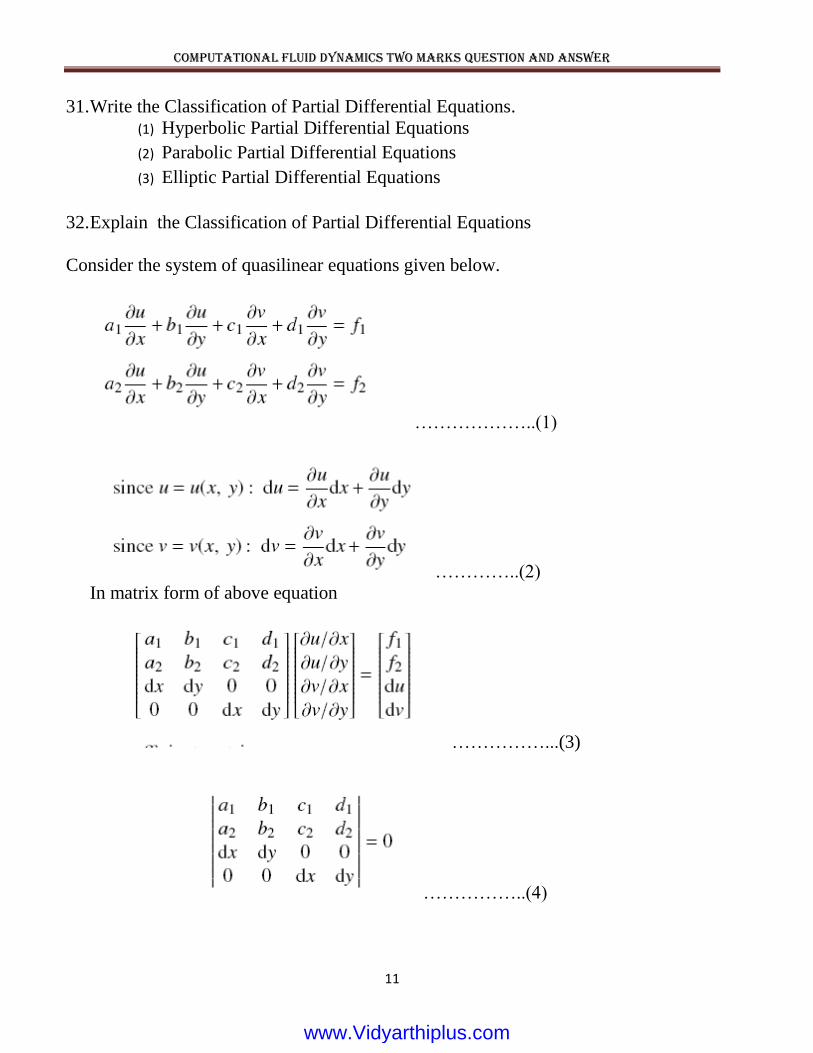
32. Explain the Classification of Partial Differential Equations

Consider the system of quasilinear equations given below.

………………..(1)

…………..(2)

In matrix form of above equation

……………...(3)

……………..(4)



12

…(5)

………………..(6)

,

The characteristic lines may be real and distinct, real and equal, or imaginary,

depending on the value of D. Specifically:

If D > 0: Two real and distinct characteristics exist through each point in the xy-

plane. When this is the case, the system of equations given by

Eqs. (1) is called hyperbolic.

If D = 0: One real characteristic exists. Here, the system of Eqs. (1) is called parabolic.

If D < 0: The characteristic lines are imaginary. Here, the system of Eqs. (1) is called

elliptic.

33. Define Well-Posed Problems?

In the solution of partial differential equations it is sometimes easy to attempt a

solution using incorrect or insufficient boundary and initial conditions. Whether the

solution is being attempted analytically or numerically, such an ‘ill-posed’ problem

will usually lead to spurious results.

Therefore, we define a well-posed problem as follows: If the solution to a partial

differential equation exists and is unique, and if the solution depends continuously



13

upon the initial and boundary conditions, then the problem is well-posed. In CFD, it is

important that you establish that your problem is well-posed before you attempt to

carry out a numerical solution.

34. Define grid point?

Analytical solutions of partial differential equations involve closed-form

expressions which give the variation of the dependent variables continuously

throughout the domain. In contrast, numerical solutions can give answers at only

discrete points in the domain, called grid points.

35. What are error influence numerical solutions the PDE?

a. Discretization error

b. Round-off error

36. Define Discretization error?

The difference between the exact analytical solution of the partial differential

equation and the exact solution of the corresponding difference equation.

Discretization error for the difference is simply the truncation error for the difference

equation plus any errors introduced by the numerical trement of the boundary

condition.

37. Define Round-off error?

The numerical error introduced after a repetitive number of calculation in which

the computer is constantly rounding the number to some significant figure.

38. Type of grid generation?

a. structured,

b. unstructured

39. How to reduce the truncation error?

The truncation error can be reduced by:

(a) Carrying more terms in the Taylor’s series, This leads to higher-order

accuracy in the representation of ui+1,j.

(b) Reducing the magnitude of Δx

40. Write the advantage of explicit approach.

Relatively simple to set up and program.



14

41. Write the Disadvantage of the explicit approach.

Given Δx, Δt must be less than some limit imposed by stability constraints. In

many cases, Δt must be very small to maintain stability; this can result in long

computer running times to make calculations over a given interval of t.

42. Write the advantage of implicit approach.

Stability can be maintained over much larger values of Δt, hence

using considerably fewer time steps to make calculations over a given interval

of t. This results in less computer time.

42. Write the advantage of implicit approach.

1. More complicated to set up and program.

2. Since massive matrix manipulations are usually required at each time step, the

computer time per time step is much larger than in the explicit approach.

3. Since large Δt can be taken, the truncation error is larger, and the use of

implicit methods to follow the exact transients (time variations of the independent

variable) may not be as accurate as an explicit approach. However, for a time-

dependent solution in which the steady state is the desired result, this relative time-

wise inaccuracy is not important.

43. What is Lax method?

………..(a)

The differencing used in the above equation, where Eq. (a) is used to represent the

time derivative, is called the Lax method.

44. Define Courant number?

(or)

What is the important stability criterion for hyperbolic equation?

C is called the Courant number. This equation says that Δt ≤ Δx/c for the numerical

solution of Eq. (5.45) to be stable. Moreover, Eq. (5.47) is called the Courant–



15

Friedrichs–Lewy condition, generally written as the CFL condition. It is an important

stability criterion for hyperbolic equations.

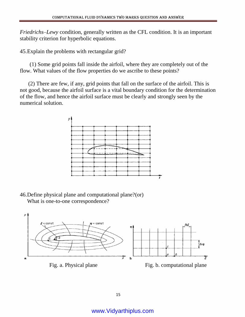
45. Explain the problems with rectangular grid?

(1) Some grid points fall inside the airfoil, where they are completely out of the

flow. What values of the flow properties do we ascribe to these points?

(2) There are few, if any, grid points that fall on the surface of the airfoil. This is

not good, because the airfoil surface is a vital boundary condition for the determination

of the flow, and hence the airfoil surface must be clearly and strongly seen by the

numerical solution.

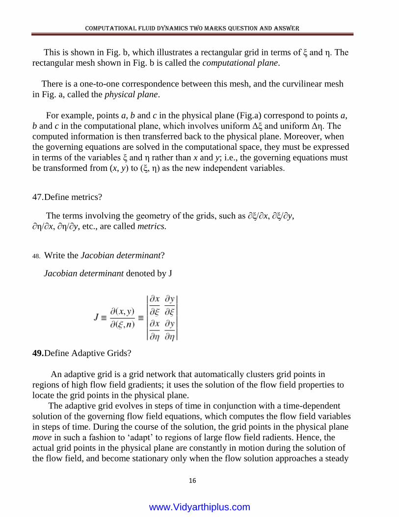
46. Define physical plane and computational plane?(or)

What is one-to-one correspondence?

Fig. a. Physical plane Fig. b. computational plane



16

This is shown in Fig. b, which illustrates a rectangular grid in terms of ξ and η. The

rectangular mesh shown in Fig. b is called the computational plane.

There is a one-to-one correspondence between this mesh, and the curvilinear mesh

in Fig. a, called the physical plane.

For example, points a, b and c in the physical plane (Fig.a) correspond to points a,

b and c in the computational plane, which involves uniform Δξ and uniform Δη. The

computed information is then transferred back to the physical plane. Moreover, when

the governing equations are solved in the computational space, they must be expressed

in terms of the variables ξ and η rather than x and y; i.e., the governing equations must

be transformed from (x, y) to (ξ, η) as the new independent variables.

47. Define metrics?

The terms involving the geometry of the grids, such as ∂ξ/∂x, ∂ξ/∂y,

∂η/∂x, ∂η/∂y, etc., are called metrics.

48. Write the Jacobian determinant?

Jacobian determinant denoted by J

49. Define Adaptive Grids?

An adaptive grid is a grid network that automatically clusters grid points in

regions of high flow field gradients; it uses the solution of the flow field properties to

locate the grid points in the physical plane.

The adaptive grid evolves in steps of time in conjunction with a time-dependent

solution of the governing flow field equations, which computes the flow field variables

in steps of time. During the course of the solution, the grid points in the physical plane

move in such a fashion to ‘adapt’ to regions of large flow field radients. Hence, the

actual grid points in the physical plane are constantly in motion during the solution of

the flow field, and become stationary only when the flow solution approaches a steady



17

state. Where the generation of the grid is completely separate from the flow field

solution, an adaptive grid is intimately linked to the flow field solution, and changes as

the flow field changes.

Fig. Adapted grid for the rearward-facing step problem

50. Write the advantages of adaptive grid?

An adaptive grid is expected because the grid points are clustered in regions

where the ‘action’ is occurring.

These advantages are:

(1) Increased accuracy for a fixed number of grid points, or

(2) For a given accuracy, fewer grid points are needed.

51. What are the topologies used in grid generation?

C-Grid Topology

O-Grid Topology

H-Grid Topology

51. Define Unstructured Grids?

Unstructured grids are typically composed of triangles in 2D and of tetrahedral in

3D.

52. Define mixed element grids?

Nowadays it becomes increasingly popular to build unstructured grids from

various element types. For example, hexahedra or prisms are employed to discretise

boundary layers. The rest of the flow domain is filled with tetrahedra. Pyramids are

used as transitional elements between the hexahedra or the prisms and the

tetrahedral. Hence the name mixed element grids.



18

53. Write the unstructured grid generation methodology.

Unstructured grid generation methodologies for CFD applications are mostly

based on either an

(1) Delaunay, method. or

(2) Advancing-front method.

54. Define Dirichlet tessellatipn or Voronoj diagram?

The Delaunay triangulation is based on a methodology proposed by Dirichlet in

1850 for the unique subdivision of space into a set of packed convex regions. Given a

set of points, each region represents the space around the particular point, which is

closer to that point than to any other. The regions form polygons (polyhedra in 3D)

which are known as the Dirichlet tessellation or the Voronoj diagram .

55. Define Delaunay triangulation?

If we connect point pairs which share some segment(face) of the Voronoj

diagram by straight lines, we obtain the Delaunay triangulation. The triangulation

defines a set of triangles (tetrahedra in 3D),which cover the convex hull of the points.

This is displayed in Fig. a. The DeIaunay triangulation is the dual of the Voronoj

diagram. The nodes of the Voronoj polygons are in 2D the centres of circumcircles of

the triangles. In 3D, the nodes represent the centres of circumspheres of the tetrahedra.

This implies that the circumcircle of every triangle (circumsphere of every tetrahedron)

contains no point from the set in its interior.

56. Write the ‘Prandtl’s boundary layer equations’.



19

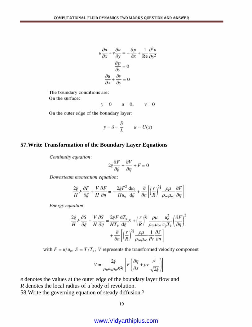
57. Write Transformation of the Boundary Layer Equations

e denotes the values at the outer edge of the boundary layer flow and

R denotes the local radius of a body of revolution.

58. Write the governing equation of steady diffusion ?



20

59. What is weak instability?

The results of the calculation are displayed in Fig.a. One notices that the

perturbation on u1 gives rise to amplifying oscillations. In fact, as small as the initial

perturbation may be - and there will always be one because of round off errors – it will

eventually lead to an explosion of the numerical solution. This phenomenon is clearly

inacceptable. It is named weak instability.

60. Define finite element method?

The finite element method (FEM) is a numerical technique for solving partial

differential equations (PDE’s).

61. Write the essential characteristic of FEM in CFD?

Its first essential characteristic is that the continuum field, or domain, is

subdivided into cells, called elements, which form a grid. The elements (in 2D) have a

triangular or a quadrilateral form and can be rectilinear or curved. The grid itself need

not be structured. With unstructured grids and curved cells, complex geometries can be

handled with ease.



21

The second essential characteristic of the FEM is that the solution of the discrete

problem is assumed a priori to have a prescribed form. The solution has to belong to a

function space, which is built by varying function values in a given way, for instance

linearly or quadratically, between values in nodal points. The nodal points, or nodes,

are typical points of the elements such as vertices, mid-side points, mid element points,

etc.

The third essential characteristic is that a FEM does not look for the solution of

the PDE itself, but looks for a solution of an integral form of the PDE. The most

general integral form is obtained from a weighted residual formulation. By this

formulation the method acquires the ability to naturally incorporate differential type

boundary conditions and allows easily the construction of higher order accurate

methods. The ease in obtaining higher order accuracy and the ease of implementation

of boundary conditions form a second important advantage of the FEM. With respect

to accuracy. The FEM is superior to the FVM, where higher order accurate

formulations are quite complicated.

A final essential characteristic of the FEM is the modular way in which the

discretization is obtained. The discrete equations are constructed from contributions on

the element level which afterwards are assembled.

62. What is the basis of FVM?

It is important that the conservation laws in their integral form are represented

accurately. The most natural method to accomplish this is to discretize the integral

form of the equations and not the differential form. This is the basis of a finite volume

method.

63. Define cell?

The flow field or domain is subdivided, as in the finite element method, into a set

of non-overlapping cells that cover the whole domain. In the finite volume Method

(FVM) the term cell is used instead of the term element used in the finite Element

method (FEM).



22

64. Define node?

The conservation laws are applied to determine the flow variables in some discrete

points of the cells, called nodes. As in the FEM, these nodes are at typical locations of

the cells, such as cell-centres, cell-vertices or mid sides

65. Define cell-centres,cell-vertices?

The choice of the nodes can be governed by the wish to represent the solution

by an interpolation structure, as in the FEM. A typical choice is then cell-centres for

representation as piecewise constant functions or cell-vertices for representation as

piecewise linear (or bilinear) functions. However, in the FVM, a function space for the

solution need not be defined and nodes can be chosen in a way that does not imply an

interpolation structure. Figure shows some typical examples of choices of nodes with

the associated definition of variables.

66. Define staggered grid approach?

A typical choice is then cell-centres for representation as piecewise constant

functions or cell-vertices for representation as piecewise linear (or bilinear) functions.

choices imply an interpolation structure, the last two do not. In the last example,

function values are not defined in all nodes. The grid of nodes on which pressure and

density are defined is different from the grid of nodes on which velocity-x components

and velocity-y components are defined. This approach commonly is called the

staggered grid approach.



23

67. What is the formulation the FVM?

The finite volume method (FVM) tries to combine the best from the finite element

method (FEM), i.e. the geometric flexibility, with the best of the finite difference

method (FDM), i.e. the flexibility in defining the discrete flow field (discrete values of

dependent variables and their associated fluxes).

68. What is Lax-Wendroff time-stepping?

Lax-Wendroff time-stepping is a very classic explicit time integration method

in the finite difference method the principles of a Lax-Wendroff method with the use

of the onedimensional scalar model equation

69. What is CFD?

CFD is the simulation of fluids engineering systems using modeling

(mathematical physical problem formulation) and numerical methods (discretization

methods, solvers, numerical parameters, and grid generations, etc.)

Historically only Analytical Fluid Dynamics (AFD) and Experimental Fluid

Dynamics (EFD).CFD made possible by the advent of digital computer and

advancing with improvements of computer resources (500 flops, 1947�20

teraflops, 2003)

70. Why use CFD?

• Analysis and Design

1. Simulation-based design instead of “build & test” More cost effective and

more rapid than EFD CFD provides high-fidelity database for diagnosing flow

field

2. Simulation of physical fluid phenomena that are difficult for experiments

�Full scale simulations (e.g., ships and airplanes) Environmental effects (wind,

weather, etc.) Hazards (e.g., explosions, radiation, pollution)Physics (e.g., planetary

boundary layer, stellar evolution)

• Knowledge and exploration of flow physics



24

71. Where is CFD used?

Aerospace, Automotive, Biomedical, Chemical, Processing, HVAC, Hydraulics,

Marine, Oil & Gas, Power Generation, Sports.

72. What are the Commercial Software for CFD?

The market is currently dominated by four codes:

1) PHOENICS

2) FLUENT

3) FLOW3D

4) STAR-CD

73. What are the Advantages of CFD over EFD?

• Substantial reduction of lead times and costs of new designs.

• Ability to study systems where controlled experiments are difficult or

impossible to perform (e.g. very large systems).

• Ability to study systems under hazardous conditions at and beyond their

normal performance limits (e.g. safety studies and accident scenarios).

• Practically unlimited level of detail of results.


what are the fundamental governing equations of fluid

Documents