weyl multifractional ornstein uhlenbeck processes mixed
TRANSCRIPT

PROBABILITYAND
MATHEMATICAL STATISTICS
Vol. 40, Fasc. 2 (2020), pp. 269–295Published online 9.7.2020
doi:10.37190/0208-4147.40.2.5
WEYL MULTIFRACTIONAL ORNSTEIN–UHLENBECK PROCESSESMIXED WITH A GAMMA DISTRIBUTION
BY
KHALIFA E S - S E BA I Y (KUWAIT CITY),FATIMA-EZZAHRA FA R A H (MARRAKESH), AND ASTRID H I L B E RT (VÄXJÖ)
Abstract. The aim of this paper is to study the asymptotic behavior of ag-gregated Weyl multifractional Ornstein–Uhlenbeck processes mixed withGamma random variables. This allows us to introduce a new class of pro-cesses, Gamma-mixed Weyl multifractional Ornstein–Uhlenbeck processes(GWmOU), and study their elementary properties such as Hausdorff dimen-sion, local self-similarity and short-range dependence. We also prove thatthese processes approach the multifractional Brownian motion.
2020 Mathematics Subject Classification: Primary 60G22; Secondary60G17.
Key words and phrases: Weyl multifractional Ornstein–Uhlenbeck pro-cess, Gamma distribution, aggregated process, multifractional Brownianmotion.
1. INTRODUCTION
Fractional Ornstein–Uhlenbeck (fOU) processes are one of the most well studiedand widely applied classes of stochastic processes [8]. Recently, in [10], an inter-esting class of processes, of interest for various applications, has been introducedemploying sequences of fOU processes with random coefficients.
Let us first present a brief summary of their construction. Let BH =BH(t), t ∈ R be a fractional Brownian motion (fBm) with Hurst indexH > 1/2, defined on a probability space (ΩBH ,FBH ,PBH ). Consider a sequenceof stationary fOU processes Xk, k 1, with random coefficients defined by thestochastic integral
(1.1) Xkt =
t∫−∞
eγk(t−s) dBHs , t ∈ R,
with initial condition Xk0 =
∫ 0
−∞ eγk(t−s) dBH
s . The random coefficients
© Probability and Mathematical Statistics, 2020

270 K. Es-Sebaiy et al.
γk, k 1, are independent random variables on a probability space (Ωγ ,Fγ ,Pγ)and for any k 1, −γk ∼ Γ(1− h, λ) with 0 < h < 1−H and λ > 0.
Assume that the family γk, k 1 is independent of BH . The processesXk, k 1, defined above are Pγ-almost surely fOU processes (see [8]). Let
(1.2) Yn(t) =1
n
n∑k=1
Xk(t), t ∈ R,
denote the so-called aggregated process. It has been proven that as n → ∞,(Yn)n1 converges weakly and in L2(ΩBH ) for fixed time, Pγ-almost surely toa stochastic process denoted by Y λ := Y λ(t), t ∈ R, given by the stochasticintegral
(1.3) Y λ(t) =t∫−∞
(λ
λ+ t− s
)1−hdBH
s , t ∈ R.
The limiting process Y λ is stationary, almost self-similar and exhibits long-rangedependence (see [13] or [10]). The asymptotic behavior of Y λ with respect to λhas also been studied, as λ varies between∞ and 0. The process Y λ ranges froma fBm with index H to a fBm with index h+H .
When BH is a standard Brownian motion (i.e. H = 1/2), Gamma-mixedOrnstein–Uhlenbeck processes have been studied in [13].
Our goal is to construct a new kind of processes, called Gamma-mixed Weylmultifractional Ornstein–Uhlenbeck (GWmOU) processes, in analogy to the lim-iting procedure that leads to the process defined in (1.3). In our construction wereplace the processes Xk, 1 ¬ k ¬ n, in the aggregated process (1.2) by Weylmultifractional Ornstein–Uhlenbeck (WmOU) processes mixed with Gamma ran-dom variables defined by the Wiener integral
Xkα(t)(t) =
1
Γ(α(t))
t∫−∞
(t− s)α(t)−1eγk(t−s) dBs, t ∈ R,
whereB = B(s), s ∈ R is a Brownian motion on (ΩB,FB, PB), and γk, k 1,are independent random variables on (Ωγ ,Fγ , Pγ), also independent of B, and forany k 1, −γk ∼ Γ(1 − h, λ) with 0 < h < 1 and λ > 0. Moreover, α is aHolder continuous function with exponent 0 < β ¬ 1. The processes Xk, k 1,are Pγ-almost surely WmOU processes (see Section 2).
We define a GWmOU, denoted Y λα , by
Y λα(t)(t) =
1
Γ(α(t))
t∫−∞
(λ
λ+ t− s
)1−h(t− s)α(t)−1 dBs, t ∈ R.
It is non-stationary, locally asymptotically self-similar and exhibits short-range de-pendence. We will also study the Holder exponent and the box and Hausdorff di-mension of the process Y λ
α . In addition, we will investigate the asymptotic behav-ior of Y λ
α with respect to λ; we will prove that Y λα approaches the multifractional

Gamma-mixed multifractional processes 271
Brownian motion (see [17]) as λ→∞, while its integrated renormalized process
Y λα (t) = λh−1
t∫0
Y λα (s) ds, t 0,
(here we suppose that the function α is constant) converges to a fractional Brown-ian motion modulo a constant as λ→ 0.
The motivation of this work comes from two facts. On the one hand, Gamma-mixed processes are good models for various applications; for example, the limit-ing process Y λ defined by (1.3) is a successful model of heart rate variability andcould also be a good model of a lot of Gaussian stationary data with long-range de-pendence (see [10], [13] for more details). Moreover, the so-called Gamma-mixedPoisson processes (also named Polya processes) have many practical applications,one of them being the study of reliability of engineering systems [9]. On the otherhand, multifractional Ornstein–Uhlenbeck processes are omnipresent in physics.For further details and references, we refer the reader to [15]. Also, for more detailsabout the construction and study of several classes of multifractional processes,see e.g. [3], [2], [5], [4], [17], [19]. The above motivate mixing multifractionalOrnstein–Uhlenbeck processes (Weyl version) with Gamma random variables, inorder to introduce GWmOU processes, as a counterpart of the limiting processY λ, a new candidate to model several short range, variable fractal dimension andnon-stationary physical phenomena.
The paper is structured as follows. Section 2 presents a short summary of re-sults on WmOU processes. In Section 3 we introduce GWmOU processes as lim-its of aggregated Weyl multifractional Ornstein–Uhlenbeck processes mixed withGamma-distributed random variables. Finally, Section 4 contains some interestingproperties of GWmOU processes including their asymptotic behavior.
2. PRELIMINARIES
WmOU processses have been introduced as a multifractional generalization ofWeyl fractional Ornstein–Uhlenbeck processes (WfOU).
Let us begin with a brief review of WfOU processes (see [14]). First, we recallsome elementary definitions of fractional calculus (see [16], [18]). The Weyl frac-tional derivative of order α > 0, denoted by aD
αt , for a = −∞, can be defined by
its inverse using the Weyl fractional integral,
aD−αt f(t) = aI
αt f(t) =
1
Γ(α)
t∫a
(t− s)α−1f(s) ds, t a.
For n − 1 ¬ α < n, aDαt is defined as the ordinary derivative of order n of the
Weyl fractional integral of order n− α,
aDαt = (d/dt)n aD
α−nt .

272 K. Es-Sebaiy et al.
WfOUs are stochastic processes obtained as solutions of the fractional Langevinequation
(aDt + w)αX(t) = W (t), α > 0, w > 0,
whereW (t) is a Gaussian white noise. They are defined explicitly by the stochasticintegral
Xα(t) =1
Γ(α)
t∫−∞
(t− s)α−1e−w(t−s) dBs, t ∈ R,
where B = B(s), s ∈ R is the standard Brownian motion and α > 1/2 toensure that Xα(t) has finite variance.
Similarly to the generalization of fractional Brownian motion to multifractionalBrownian motion (see [17]), an extension of WfOU processes is obtained by re-placing the parameter α by a Holder continuous function with exponent 0 < β ¬ 1,i.e. there exists a constant K such that
|α(t)− α(s)| ¬ K|t− s|β ∀s, t,
and α(t) > 1/2 for all t.Let us recall WmOU processes and their properties needed in what follows. For
more details we refer the reader to [15].A WmOU process is a Gaussian process defined by the Wiener integral
Xα(t)(t) =1
Γ(α(t))
t∫−∞
(t− s)α(t)−1e−w(t−s) dBs, t ∈ R.
We have
(2.1) EB[(Xα(t)(t+ s)−Xα(t)(t))2]
=−|s|2α(t)−1
Γ(2α(t)) cos(πα(t))− 2|s|2w3−2α(t)Sα(t)(w|s|),
where Sϑ(x) is a continuous function given explicitly by
Sϑ(x) = −√π
8Γ(ϑ) cos(πϑ)
[ ∞∑m=0
x2m
22m(m+ 1)!Γ(m+ 5/2− ϑ)
−(x
2
)2ϑ−1 ∞∑m=0
x2m
22m(m+ 1)!Γ(m+ 3/2 + ϑ)
]for every x > 0 and 1/2 < ϑ < 3/2. The relevant variance is equal to
E[Xα(t)(t)2] =
(2w)1−2α(t)Γ(2α(t)− 1)
Γ(α(t))2.

Gamma-mixed multifractional processes 273
On the other hand, for s < t the covariance of the WmOU is given by
E[Xα(t)(t)Xα(s)(s)]
=e−w(t−s)(t− s)α(t)+α(s)−1
Γ(α(t))ψ(α(s), α(s) + α(t); 2w(t− s)
),
where ψ(α, γ; z) is the confluent hypergeometric function. The variance and thecovariance functions are divergent when w → 0. However, if we set Zα(t)(t) =Xα(t)(t) −Xα(t)(0), it has been proven in [15] that for α(t) ∈ (1/2, 3/2) and byidentifying α(t) withH(t)+1/2,whenw → 0 the process Zα(t)(t) approaches (inthe sense of finite-dimensional distributions) BH(t)(t), the multifractional Brown-ian motion (with moving average definition) defined in [17] by
BH(t)(t) =1
Γ(H(t) + 1/2)
×( 0∫−∞
[(t− s)H(t)−1/2 − (−s)H(t)−1/2] dBs +t∫0
(t− s)H(t)−1/2 dBs
).
For the basic properties of WmOU processes such as short-range dependence, localself-similarity and Hausdorff dimension, we refer the reader to [15].
Let us now recall a sufficient criterion for weak convergence, which will beneeded in what follows. By Prokhorov’s theorem, the convergence of finite-di-mensional distributions and tightness yield weak convergence. For processes X ,Xn, n 1, with paths in C([a, b],R), one has the following sufficient criterion(Billingsley [6, Theorem 12.3], or [7]).
THEOREM 2.1. Suppose that the finite-dimensional distributions of the family(Xn)n1 converge to those of X . If, in addition, there exist constants ζ > 0, θ > 1and cζ,θ, depending only on ζ and θ, such that for all s, t ∈ [a, b] with a,b ∈ R,a < b,
E[|Xn(t)−Xn(s)|ζ ] ¬ cζ,θ|t− s|θ
for all n 1, then the family (Xn)n1 is tight and consequently
Xn → X weakly in C[a, b] as n→∞.
3. AGGREGATED WEYL MULTIFRACTIONAL ORNSTEIN–UHLENBECK PROCESSESMIXED WITH GAMMA DISTRIBUTION
Let us now consider a sequence of WmOU processes mixed with Gamma distribu-tion random variables Xk
α := Xkα(t)(t), t ∈ R defined by the following Wiener
integral:
(3.1) Xkα(t)(t) =
1
Γ(α(t))
t∫−∞
(t− s)α(t)−1eγk(t−s) dBs, t ∈ R,

274 K. Es-Sebaiy et al.
where B = B(s), s ∈ R is a Brownian motion defined on a probability space(ΩB,FB, PB) and for any k 1, −γk ∼ Γ(1 − h, λ) with 0 < h < 1 and λ > 0are independent random variables, also independent of B, defined on a probabilityspace (Ωγ ,Fγ , Pγ).
The processes Xkα, k 1, are Pγ-almost surely WmOU processes defined on
(ΩB,FB, PB). We define their empirical mean by
Y nα(t)(t) =
1
n
n∑k=1
Xkα(t)(t)
for every t ∈ R and n 1.Throughout the paper we assume that
(3.2) 1/2 < αinf ¬ αsup < 3/2,
where αinf := inft∈R α(t) and αsup := supt∈R α(t).We will also need the following notations:
• mα[a, b] = minα(t) : t ∈ [a, b] and Mα[a, b] = maxα(t) : t ∈ [a, b] forall real a < b. EB and Eγ denote the expectations with respect to PB and Pγrespectively.
• C denotes a generic constant depending only on [a, b], λ and h.
• Cx,y denotes a generic constant depending on [a, b], λ, h, x and y such that0 < x < 2mα[a, b]− 1 and 0 < y < 3/2− h−Mα[a, b].
• Cx,yη denotes a generic constant depending on [a, b], λ, h, x and y such that0 < x < 2mα[a, b]−1, 0 < y < 3/2−h−Mα[a, b] and 0 ¬ η < mα[a, b]−1/2.
3.1. The limit of aggregated processes. If 0 < h < 3/2 − αsup, we define a zeromean Gaussian process Y λ
α := Y λα(t)(t), t ∈ R by
(3.3) Y λα(t)(t) =
1
Γ(α(t))
t∫−∞
(λ
λ+ t− s
)1−h(t− s)α(t)−1 dBs, t ∈ R.
It is easy to see that the Wiener integral in (3.3) is well-defined. The process Y λα
will be called a Gamma-mixed Weyl multifractional Ornstein–Uhlenbeck process,abbreviated as GWmOU.
Given a compact interval [a, b] ⊂ R, the following result proves that Pγ-a.s.,as n→∞, Y n
α(t)(t) converges to Y λα(t)(t) in L2(ΩB), uniformly in t ∈ [a, b].
THEOREM 3.1. Fix real numbers a, b such that a < b. If 0 < h < 3/2 −Mα[a, b], then Pγ-a.s.,
(3.4) Y nα(t)(t) −−−→n→∞
Y λα(t)(t) in L2(ΩB)

Gamma-mixed multifractional processes 275
uniformly in t ∈ [a, b]. In particular, if 0 < h < 3/2−αsup, then Pγ-a.s., for everyt ∈ R,
(3.5) Y nα(t)(t) −−−→n→∞
Y λα(t)(t) in L2(ΩB).
Proof. We prove (3.4). For every x > 0, n 1, set
fn(x) :=1
n
n∑k=1
eγkx, c(x) := Eγ [eγ1x] =
(λ
λ+ x
)1−h.
By the law of large numbers, we have Pγ-a.s., for every x > 0,
(3.6) fn(x) =1
n
n∑k=1
eγkx −−−→n→∞
c(x),
and for every c > 0 and d < 3/2− h,
(3.7)1
n
n∑k=1
eγkc
(−γk)d−1/2−−−→n→∞
Eγ
[eγ1c
(−γ1)d−1/2
]=
λ1−hΓ(3/2− d− h)
Γ(1− h)(λ+ c)3/2−d−h .
Using the change of variable u = t− s, we can write
EB[(Y nα(t)(t)− Y
λα(t)(t))
2]
=1
Γ(α(t))2EB
[( t∫−∞
(t− s)α(t)−1(fn(t− s)− c(t− s)
)dBs
)2]=
1
Γ(α(t))2
t∫−∞
(t− s)2α(t)−2(fn(t− s)− c(t− s)
)2ds
=1
Γ(α(t))2
∞∫0
u2α(t)−2(fn(u)− c(u))2 du.
Hence, for every m 2 and t ∈ [a, b],
(3.8) EB[(Y nα(t)(t)− Y
λα(t)(t))
2]
=1
Γ(α(t))2
[ 1∫0
u2α(t)−2(fn(u)− c(u))2du+m∫1
u2α(t)−2(fn(u)− c(u))2 du
+∞∫m
u2α(t)−2(fn(u)− c(u))2 du]
¬ K[ 1∫
0
u2mα[a,b]−2(fn(u)− c(u))2du+m∫1
u2Mα[a,b]−2(fn(u)− c(u))2 du
+∞∫m
u2Mα[a,b]−2(fn(u)− c(u))2 du]
:= K[A(n,m) +B(n,m) + C(n,m)],

276 K. Es-Sebaiy et al.
where K is the maximum of the continuous function z 7→ 1/Γ(z) on the interval[mα[a, b],Mα[a, b]].
Combining (3.6), fn(u) ¬ 1, c(u) ¬ 1 and (3.2) with Lebesgue’s dominatedconvergence theorem, we conclude that Pγ-a.s, for every m 2,
(3.9) A(n,m) −−−→n→∞
0, B(n,m) −−−→n→∞
0.
Now we will estimate C(n,m) for all m 2. We have
C(n,m) =∞∫m
(fn(u)− c(u))2u2Mα[a,b]−2 du
¬ 2∞∫m
fn(u)2u2Mα[a,b]−2 du+ 2∞∫m
c(u)2u2Mα[a,b]−2 du.
Moreover, by the change of variable v = (−γj − γk)u and 2√
(−γj)(−γk) ¬−γj − γk,
∞∫m
fn(u)2u2Mα[a,b]−2 du =1
n2
n∑k,j=1
∞∫m
eγjueγkuu2Mα[a,b]−2 du
=1
n2
n∑k,j=1
1
(−γj − γk)2Mα[a,b]−1
∞∫m(−γj−γk)
v2Mα[a,b]−2e−v dv
¬ 21−2Mα[a,b]
n2
n∑k,j=1
e−m2
(−γj−γk)
[(−γj)(−γk)]Mα[a,b]−1/2
∞∫m(−γj−γk)
v2Mα[a,b]−2e−v/2 dv
¬ Γ(2Mα[a, b]− 1)
(1
n
n∑j=1
e−m2
(−γj)
(−γj)Mα[a,b]−1/2
)2
.
Combining this with (3.7) we get, Pγ-a.s.,
lim supn→∞
∞∫m
fn(u)2u2Mα[a,b]−2 du
¬ Γ(2Mα[a, b]− 1)
(λ1−hΓ(3/2−Mα[a, b]− h)
Γ(1− h)(λ+m/2)3/2−Mα[a,b]−h
)2
−−−→m→∞
0.
On the other hand, since
∞∫0
(λ
λ+ u
)2−2h
u2Mα[a,b]−2 du
= λ2Mα[a,b]−1β(3− 2Mα[a, b]− 2h, 2Mα[a, b]− 1) <∞,

Gamma-mixed multifractional processes 277
we have
∞∫m
c(u)2u2Mα[a,b]−2 du =∞∫m
(λ
λ+ u
)2−2h
u2Mα[a,b]−2 du −−−→m→∞
0.
which implies that Pγ-a.s.,
(3.10) lim supn→∞
C(n,m) −−−→m→∞
0.
Therefore, by applying the convergences (3.9) and (3.10) in (3.8) we deduce thatPγ-a.s.,
lim supn→∞
supt∈[a,b]
EB[(Y nα(t)(t)− Y
λα(t)(t))
2] = 0,
which finishes the proof of (3.4).Finally, the convergence (3.5) is a direct consequence of (3.4), (3.2) and 0 <
h < 3/2− αsup.
The weak convergence of the sequence (Y nα )n1 is established in our next the-
orem.
THEOREM 3.2. Fix real a < b. Suppose that 0 < h < 3/2 −Mα[a, b] andmin2mα[a, b]− 1, 2β < 1. Then Pγ-a.s.,
(3.11) Y nα −−−→n→∞
Y λα in C[a, b],
where C[a, b] is the space of continuous functions on [a, b].
Proof. First, since Pγ-almost surely, Y nα and Y λ
α are zero mean Gaussian pro-cesses whose finite-dimensional distributions are determined by their covariances,(3.4) implies the convergence Pγ-almost surely of the finite-dimensional distribu-tions of (Y n
α )n1 to those of Y λα . Thus, in order to prove (3.11) it remains to prove
the Pγ-a.s. tightness of (Y nα )n1 by using Theorem 2.1.
Throughout the proof all the results are given Pγ-almost surely.Let t, t+ τ ∈ [a, b] be such that |τ | < min(λ/2, 1). Then
(3.12) EB[(Y nα(t+τ)(t+ τ)− Y n
α(t)(t))2]
= EB
[(1
n
n∑k=1
(Xkα(t+τ)(t+ τ)−Xk
α(t)(t))
)2]¬ 2EB
[(1
n
n∑k=1
Ukt (τ)
)2]+ 2EB
[(1
n
n∑k=1
V kt (τ)
)2],
where
Ukt (τ) := Xkα(t)(t+ τ)−Xk
α(t)(t), V kt (τ) := Xk
α(t+τ)(t+ τ)−Xkα(t)(t+ τ).

278 K. Es-Sebaiy et al.
We will first prove that for every n 1,
(3.13) EB
[(1
n
n∑k=1
Ukt (τ)
)2]¬ C|τ |2mα[a,b]−1.
To this end, by using Holder’s inequality and (2.1), we can write
EB
[(1
n
n∑k=1
Ukt (τ)
)2]¬ 1
n
n∑k=1
EB[Ukt (τ)2]
=−|τ |2α(t)−1
Γ(2α(t)) cos(πα(t))− 2|τ |2 1
n
n∑k=1
(−γk)3−2α(t)Sα(t)(−γk|τ |).
Since 1/2 < α(t) < 3/2 and cos(πα(t)) < 0, we get
−Sα(t)(−γk|τ |)
=
√π
8Γ(α(t)) cos(πα(t))
∞∑m=0
(−γk|τ |)2m
22m(m+1)!Γ(m+5/2−α(t))
−√π
8Γ(α(t)) cos(πα(t))
(−γk|τ |
2
)2α(t)−1 ∞∑m=0
(−γk|τ |)2m
22m(m+1)!Γ(m+3/2+α(t))
¬ −√π
8Γ(α(t)) cos(πα(t))
(−γk|τ |
2
)2α(t)−1 ∞∑m=0
(−γk|τ |)2m
22m(m+1)!Γ(m+3/2+α(t))
¬ C(−γk|τ |)2α(t)−1∞∑m=0
(−γk|τ |)2m
22m((m+1)!)2,
where the last inequality comes from Γ(m + 3/2 + α(t)) (m + 1)! and thefact that the functions Γ(x) and cos(πx) are continuous at every x with 1/2 <mα[a, b] ¬ x ¬Mα[a, b] < 3/2.
As a consequence,
(3.14) EB
[(1
n
n∑k=1
Ukt (τ)
)2]¬ C|τ |2α(t)−1
(1 +
1
n
n∑k=1
(−γk)2∞∑m=0
(−γk|τ |)2m
22m((m+ 1)!)2
).
Moreover, by the law of large numbers, we obtain
(3.15) limn→∞
1
n
n∑k=1
(−γk)2∞∑m=0
(−γk|τ |)2m
22m((m+ 1)!)2
= Eγ
[(−γ1)2
∞∑m=0
(−γ1|τ |)2m
22m((m+1)!)2
]=
1
Γ(1−h)λ2
∞∑m=0
Γ(2m+3−h)
22m((m+1)!)2
(|τ |λ
)2m
¬ C∞∑m=0
Γ(2m+3−h)
22m((m+1)!)2
(1
2
)2m
<∞,

Gamma-mixed multifractional processes 279
where we have used the fact that the radius of convergence of the power series∑∞m=0
Γ(2m+3−h)22m((m+1)!)2
xm is 1. By combining (3.14) and (3.15), we obtain (3.13).Let us now turn to the second term in (3.12). It remains to prove that for every
n 1,
EB
[(1
n
n∑k=1
V kt (τ)
)2]¬ Cδ,ρ|τ |2β.(3.16)
To this end, from (3.1) we can write
(3.17) V kt (τ) = V k
t,1(τ) + V kt,2(τ),
where
V kt,1(τ) =
(1
Γ(α(t+ τ))− 1
Γ(α(t))
) t+τ∫−∞
(t+ τ −u)α(t+τ)−1eγk(t+τ−u) dBu,
V kt,2(τ) =
1
Γ(α(t))
t+τ∫−∞
((t+ τ −u)α(t+τ)−1− (t+ τ −u)α(t)−1
)eγk(t+τ−u) dBu.
Then
EB
[(1
n
n∑k=1
V kt (τ)
)2]¬ 2EB
[(1
n
n∑k=1
V kt,1(τ)
)2]+ 2EB
[(1
n
n∑k=1
V kt,2(τ)
)2].
Combining the mean value theorem and the fact that any continuous function hasa maximum on any compact interval, we get∣∣∣∣ 1
Γ(α(t+ τ))− 1
Γ(α(t))
∣∣∣∣2Γ(2α(t+ τ)− 1) ¬ C|α(t+ τ)− α(t)|2.
Moreover, since α is β-Holder continuous, and since 2√
(−γj)(−γk) ¬ −γj −γkand 1− 2α(t+ τ) < 0, we have
EB
[(1
n
n∑k=1
V kt,1(τ)
)2]=
(1
Γ(α(t+τ))− 1
Γ(α(t))
)2 1
n2
n∑j,k=1
t+τ∫−∞
(t+τ−u)2α(t+τ)−2e(γj+γk)(t+τ−u) du
=
(1
Γ(α(t+τ))− 1
Γ(α(t))
)2
Γ(2α(t+τ)−1)1
n2
n∑j,k=1
(−γj−γk)1−2α(t+τ)
¬ C|τ |2β[
1
n
n∑k=1
(−γk)1/2−α(t+τ)
]2
.

280 K. Es-Sebaiy et al.
Moreover,
1
n
n∑k=1
(−γk)1/2−α(t+τ) −−−→n→∞
λα(t+τ)−1/2
Γ(1− h)Γ(3/2− α(t+ τ)− h) <∞.
Thus, we conclude that for every n 1,
(3.18) EB
[(1
n
n∑k=1
V kt,1(τ)
)2]¬ C|τ |2β.
On the other hand, by the change of variable t+ τ − u = x, we have
EB
[(1
n
n∑k=1
V kt,2(τ)
)2]=
1
Γ(α(t))2
1
n2
×n∑
j,k=1
t+τ∫−∞
[(t+ τ − u)α(t+τ)−1 − (t+ τ − u)α(t)−1]2e(γj+γk)(t+τ−u) du
=1
Γ(α(t))2
1
n2
n∑j,k=1
∞∫0
[xα(t+τ)−1 − xα(t)−1]2e(γj+γk)x dx
=[α(t+ τ)− α(t)]2
Γ(α(t))2
1
n2
n∑j,k=1
∞∫0
[log(x)xcxt,τ−1]2e(γj+γk)x dx
for some cxt,τ ∈ (mα[a, b],Mα[a, b]), where the last equality comes from the meanvalue theorem.
Let 0 < δ < 2mα[a, b] − 1, 0 < ρ < 3/2 −Mα[a, b] − h and define µ =1/(2mα[a, b]− 1− δ). Since α is β-Holder continuous, we can write
EB
[(1
n
n∑k=1
V kt,2(τ)
)2]=
[α(t+ τ)− α(t)]2
Γ(α(t))2
1
n2
n∑j,k=1
∞∫0
log(x)2x2cxt,τ−2e(γj+γk)x dx
=[α(t+ τ)− α(t)]2
Γ(α(t))2
1
n2
n∑j,k=1
( 1∫0
log(x)2x2cxt,τ−2e(γj+γk)x dx
+∞∫1
log(x)2x2cxt,τ−2e(γj+γk)x dx)
¬ C|τ |2β( 1∫
0
x2mα[a,b]−2−δ dx+1
n2
n∑j,k=1
∞∫1
x2Mα[a,b]−2+2ρe(γj+γk)x dx
)¬ C|τ |2β
(µ+
1
n2
n∑j,k=1
∞∫0
x2Mα[a,b]−2+2ρe(γj+γk)x dx
)

Gamma-mixed multifractional processes 281
¬ C|τ |2β(µ+
1
n2
n∑j,k=1
Γ(2Mα[a, b]−1+2ρ)
(−γj−γk)2Mα[a,b]−1+2ρ
)¬ C|τ |2β
(µ+
21−2ρ−2Mα[a,b]
n2
n∑j,k=1
Γ(2Mα[a, b]−1+2ρ)
(√
(−γj)(−γk))2Mα[a,b]−1+2ρ
)= C|τ |2β
×(µ+21−2ρ−2Mα[a,b]Γ(2Mα[a, b]−1+2ρ)
(1
n
n∑k=1
1
(−γk)Mα[a,b]−1/2+ρ
)2).
Combining this with
1
n
n∑k=1
1
(−γk)Mα[a,b]−1/2+ρ−−−→n→∞
λMα[a,b]−1/2+ρ
Γ(1− h)Γ(3/2−Mα[a, b]−h−ρ) <∞,
we deduce that for every n 1,
(3.19) EB
[(1
n
n∑k=1
V kt,2(τ)
)2]¬ Cδ,ρ|τ |2β.
Thus, combining (3.18) and (3.19), we get (3.16).Therefore, from (3.12), (3.13) and (3.16) we obtain, for every n 1,
(3.20) EB[(Y nα(t+τ)(t+ τ)− Y n
α(t)(t))2] ¬ Cδ,ρ|τ |min2mα[a,b]−1,2β.
Let a < b. For s < t ∈ [a, b], we can find 2k + 2 points u1, . . . , u2k+2 ∈ [s, t]with b − a = kminλ/2, 1 + c, 0 ¬ c < minλ/2, 1 and 0 < ui+1 − ui <minλ/2, 1 such that [t, s] =
⋃2k+2i=1 [ui, ui+1].
Using Minkowski’s inequality, (3.20) and Proposition 4.1 (because 0 <min2mα[a, b]− 1, 2β < 1 ) we conclude that for every n 1 and s, t ∈ [a, b],
EB[(Y nα(t)(t)− Y
nα(s)(s))
2] ¬ Cδ,ρ|t− s|min2mα[a,b]−1,2β.
Consequently, given r > 0 and using again the fact that Y nα is Pγ-almost surely
Gaussian, there exists a constant Cr depending only on r such that
EB[|Y nα(t)(t)− Y
nα(s)(s)|
r] = Cr(EB[(Y n
α(t)(t)− Ynα(s)(s))
2])r/2
¬ Cr(Cδ,ρ)r/2|t− s|rminmα[a,b]−1/2,β
for all n 1 and s, t ∈ [a, b]. If we choose so that rminmα[a, b]− 1/2, β > 1,Theorem 2.1, implies that the family (Y n
α )n1 is tight, as desired.

282 K. Es-Sebaiy et al.
3.2. Properties of GWmOU processes and asymptotic behavior with respect to λ.In this section we study several interesting properties of the GWmOU process Y λ
α ,such as the Holder exponent and short-range dependence. In addition, we investi-gate the asymptotic behavior of Y λ
α when λ→∞ and when λ→ 0.Let us first compute the variance and the covariance of Y λ
α . An easy computa-tion shows that for all t ∈ R the variance is given by
EB[Y λα(t)(t)
2] =λ2−2h
Γ(α(t))2
t∫−∞
(λ+ t− s)2h−2(t− s)2α(t)−2 ds(3.21)
=λ2α(t)−1
Γ(α(t))2β(3− 2h− 2α(t), 2α(t)− 1),
where β is the beta function defined by β(x, y) =∫ 1
0ux−1(1 − u)y−1 du for
x, y > 0. Hence a GWmOU process is in general not stationary.In addition, for s < t, using the change of variable z = λ/(λ + s − u), the
covariance of Y λα is given by
(3.22) EB[Y λα(t)(t)Y
λα(s)(s)]
=1
Γ(α(t))Γ(α(s))
×s∫−∞
(λ
λ+ t− u
)1−h( λ
λ+ s− u
)1−h(t− u)α(t)−1(s− u)α(s)−1 du
=λα(t)+α(s)−1
Γ(α(t))Γ(α(s))G(α(t), α(s), h, t− s/λ),
with
G(a, b, c, d) =1∫0
(1 + dz)c−1
(1 + [d− 1]z)1−a (1− z)b−1z2−[a+b]−2c dz.
In order to study the local properties of GWmOU processes we will need the fol-lowing result.
PROPOSITION 3.1. Fix a compact interval [a, b] ⊂ R.
(1) If 0 < h < 3/2−Mα[a, b], then there exists a constant Cδ,ρ such that
(3.23) EB[(Y λα(t+τ)(t+ τ)− Y λ
α(t)(t))2] ¬ Cδ,ρ|τ |min2mα[a,b]−1,2β
for all t, t+ τ ∈ [a, b] with |τ | < minλ/2, 1.
(2) If 0 < h < 3/2−Mα[a, b], Mα[a, b] < 1 and α(t)− 1/2 < β for all t, then
(a) there exist constants C2 and ε < 1 such that
(3.24) EB[(Y λα(t+τ)(t+ τ)− Y λ
α(t)(t))2] (C2/2)|τ |2Mα[a,b]−1
for all t, t+ τ ∈ [a, b] with |τ | < ε,

Gamma-mixed multifractional processes 283
(b) as τ → 0,
(3.25) EB[(Y λα(t+τ)(t+ τ)− Y λ
α(t)(t))2] = C2|τ |α(t)−1/2 +O(|τ |2α(t)−1).
Proof. The inequality (3.23) is a direct consequence of (3.20) and (3.4).Let us now prove (3.24). For convenience, for all t, t+ τ ∈ [a, b] with |τ | < 1,
we set
Uλt (τ) = Y λα(t)(t+ τ)− Y λ
α(t)(t), V λt (τ) = Y λ
α(t+τ)(t+ τ)− Y λα(t)(t+ τ)
= V λt,1(τ) + V λ
t,2(τ),
where
V λt,1(τ) =
(1
Γ(α(t+τ))− 1
Γ(α(t))
) t+τ∫−∞
(t+τ−u)α(t+τ)−1 λ1−h
(λ+t+τ−u)1−h dBu,
V λt,2(τ) =
1
Γ(α(t))
×t+τ∫−∞
[(t+τ−u)α(t+τ)−1−(t+τ−u)α(t)−1]λ1−h
(λ+t+τ−u)1−h dBu.
Hence
(3.26) EB[(Y λα(t+τ)(t+ τ)− Y λ
α(t)(t))2] EB[Uλt (τ)2] + 2EB[Uλt (τ)V λ
t (τ)]
EB[Uλt (τ)2]− 2E[Uλt (τ)2]1/2E[V λt (τ)2]1/2.
The last inequality follows from the Cauchy–Schwarz inequality. By Lemma 4.1below and the inequality (4.10), there exist constants C1 and C2 depending onlyon [a, b], λ and h such that
(3.27) C2|τ |2α(t)−1 ¬ E[(Uλt )2] ¬ C1|τ |2α(t)−1.
On the other hand,
EB[V λt (τ)2] ¬ 2
(EB[V λ
t,1(τ)2] + EB[V λt,2(τ)2]
).
A standard computation combined with the mean value theorem and the fact thatany continuous function has a maximum on any compact interval, we obtain
EB[V λt,1(τ)2]
=
(1
Γ(α(t+ τ))− 1
Γ(α(t))
)2
λ2α(t+τ)−1β(3− 2α(t+ τ)− 2h, 2α(t+ τ)− 1
)¬ C|α(t+ τ)− α(t)|2 ¬ C|τ |2β.

284 K. Es-Sebaiy et al.
Moreover, by the change of variable x = t+ τ − u, we have
EB[V λt,2(τ)2]
=λ2−2h
Γ(α(t))2
t+τ∫−∞
[(t+τ−u)α(t+τ)−1−(t+τ−u)α(t)−1]2(λ+ t+τ−u)2h−2 du
=λ2−2h
Γ(α(t))2
∞∫0
[xα(t+τ)−1−xα(t)−1]2(λ+x)2h−2 dx
=λ2−2h[α(t+τ)−α(t)]2
Γ(α(t))2
∞∫0
log(x)2x2axt,τ−2 (λ+x)2h−2 du
for some axt,τ ∈ (mα[a, b],Mα[a, b]), the last equality following from the meanvalue theorem. Let 0 < σ < 2mα[a, b]−1 and 0 < ς < 3/2−Mα[a, b]−h. Since αis β-Holder continuous, for c = 3−2h−2Mα[a, b]−2ς and d = 2Mα[a, b]−1+2ςwe have
EB[V λt,2(τ)2] =
λ2−2h[α(t+ τ)− α(t)]2
Γ(α(t))2
( 1∫0
log(x)2x2cxt,τ−2(λ+ x)2h−2 dx
+∞∫1
log(x)2x2axt,τ−2(λ+ x)2h−2 dx)
¬ C|τ |2β( 1∫
0
x2mα[a,b]−2−σ dx+∞∫1
x2Mα[a,b]−2+2ς(λ+ x)2h−2 dx)
¬ C|τ |2β(1/(2mα[a, b]− 1− σ) + β(c, d)) ¬ Cσ,ς |τ |2β.
We then deduce that
(3.28) EB[V λt (τ)2] ¬ Cσ,ς |τ |2β.
Combining (3.27), (3.28) and the Cauchy–Schwarz inequality yields
(3.29) |E[Uλt (τ)V λt (τ)]| ¬ E[Uλt (τ)2]1/2E[V λ
t (τ)2]1/2 ¬ Cσ,ς |τ |β+α(t)−1/2.
Thus, by plugging (3.27) and (3.29) in (3.26), we get
EB[(Y λα(t+τ)(t+ τ)− Y λ
α(t)(t))2] C2|τ |2α(t)−1 − Cσ,ς |τ |α(t)−1/2+β
|τ |2Mα[a,b]−1(C2 − Cσ,ς |τ |β−Mα[a,b]+1/2).
By assuming that α(t)− 1/2 ¬Mα[a, b]− 1/2 < β, the function
g : τ 7→ C2 − Cσ,ς |τ |β−Mα[a,b]+1/2
is continuous in τ and converges to C2 when τ → 0. So there exists ε > 0 suchthat g(τ) > C = C2 for |τ | < ε, which gives the inequality (3.24).

Gamma-mixed multifractional processes 285
On the other hand, by the assumption α(t) − 1/2 ¬ Mα[a, b] − 1/2 < β andusing the equivalence (4.11), (3.28) and (3.29), we immediately obtain (3.25).
In the following, we state interesting properties of GWmOU processes such ascontinuity, Holder exponent at t, Hausdorff dimension and local asymptotic self-similarity. The same properties hold for WmOU processes, the proofs of whichare based on [15, Lemma 3.1], of which Proposition 3.1 is the counterpart forGWmOU processes. Having Proposition 3.1 at hand, the proofs for GWmOU pro-cesses proceed analogously to those in [15]. Therefore, we omit them.
3.2.1. Continuity
PROPOSITION 3.2. The process Y λα(t)(t), t ∈ R admits a continuous modifi-
cation.
In the following properties: Holder exponent, Hausdorff dimension and localasymptotic self-similarity, we make the additional assumptions that α(t)−1/2 < βfor all t in the domain of α and Mα[a, b] < 1.
3.2.2. Hölder exponent
PROPOSITION 3.3. Let [a, b] ⊂ R be an interval. For any 0 ¬ η < mα[a, b]−1/2, with probability 1, there exists a constant Cδ,ρη such that
|Y λα(t)(t)− Y
λα(s)(s)| ¬ C
δ,ρη |t− s|η ∀t, s ∈ [a, b].
We now turn to the Holder continuity of GWmOU processes. Let us first recallthe following definition.
DEFINITION 3.1. A real-valued function is said to have Holder exponent β ata point t0 if
limh→0
|f(t0 + h)− f(t0)||h|γ
= 0 for any γ < β,
lim suph→0
|f(t0 + h)− f(t0)||h|γ
=∞ for any γ > β.
PROPOSITION 3.4. With probability 1, the Holder exponent of Y λα(t)(t) at a
point t0 in the domain is α(t0)− 1/2.
3.2.3. Hausdorff dimension. Let dimH A, dimB A, and dimB A denote the Haus-dorff dimension, the lower box dimension, and the upper box dimension of a set Ain Rn, respectively. Given a compact interval [a, b] ⊂ R, Gα[a, b] = (t, Y λ
α(t)(t)) :
t ∈ [a, b] stands for the graph of the process Y λα(t)(t) restricted to [a, b]. For more
information on these notions see [11]. We now formulate our result.

286 K. Es-Sebaiy et al.
PROPOSITION 3.5. Let [a, b] be an interval in the domain of definition of α.With probability 1, dimH Gα[a, b] = dimBGα[a, b] = dimBGα[a, b] = 5/2 −mα[a, b].
3.2.4. Local asymptotic self-similarity. WmOU processes are locally asymptoticallyself-similar, in the following sense defined in [4].
DEFINITION 3.2. Let X(t) be a Gaussian process. We say that X(t) is locallyasymptotically self-similar with parameter H at a point t0 if the limit process
limh→0+
X(t0 + hu)−X(t0)
hH, u ∈ R
exists and is nontrivial for every t0.
This property holds true for GWmOU processes. Before stating this result, letus first recall that a fractional Brownian motion with Hurst index H is a centeredGaussian process with covariance
E[BH(t)BH(s)] = 12 [|t|2H + |s|2H − |t− s|2H ].
PROPOSITION 3.6. For any t0 the stochastic process
limh→0+
Y λα(t0+hu)(t0 + hu)− Y λ
α(t0)(t0)
hα(t0)/2−1/4, u ∈ R
is, modulo a constant, a fractional Brownian motion with Hurst index α(t0)/2− 1/4.
3.2.5. Short-range dependence. We are now interested in the strength of the depen-dence of GWmOU processes.
DEFINITION 3.3 ([12]). Let X(t) be a Gaussian process with covariance de-noted by c(s, t) = cov(X(s), X(t)) and correlation ρ(s, t) defined by
ρ(s, t) =c(s, t)√
c(t, t)c(s, s).
We say that X(t) is long-range dependent if
∞∫0
|ρ(t, t+ τ)| dτ =∞,
and it is short-range dependent if the integral is finite.
Gamma-mixed multifractional processes 287
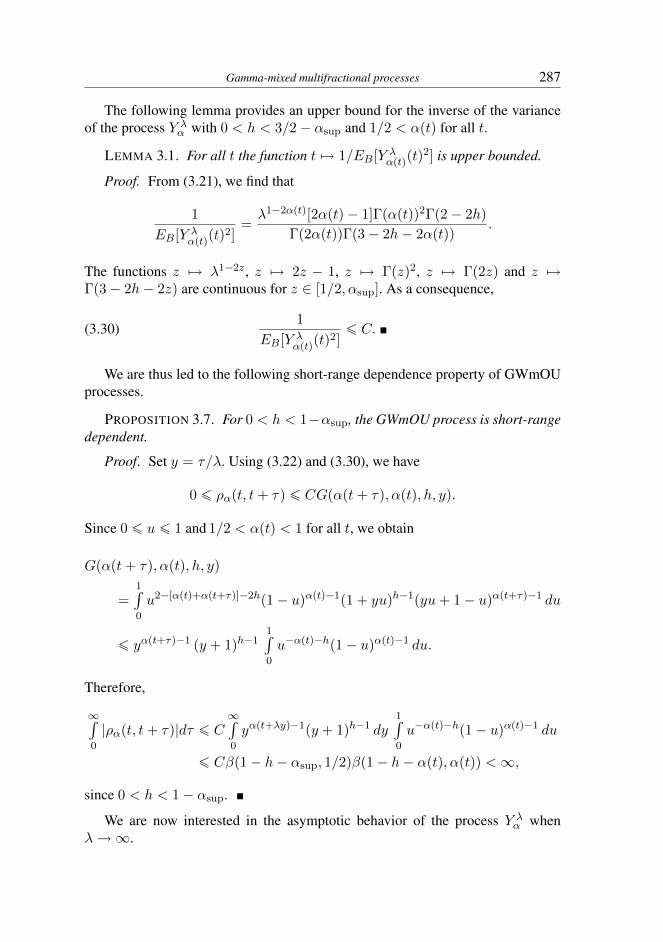
The following lemma provides an upper bound for the inverse of the varianceof the process Y λ
α with 0 < h < 3/2− αsup and 1/2 < α(t) for all t.
LEMMA 3.1. For all t the function t 7→ 1/EB[Y λα(t)(t)
2] is upper bounded.
Proof. From (3.21), we find that
1
EB[Y λα(t)(t)
2]=λ1−2α(t)[2α(t)− 1]Γ(α(t))2Γ(2− 2h)
Γ(2α(t))Γ(3− 2h− 2α(t)).
The functions z 7→ λ1−2z , z 7→ 2z − 1, z 7→ Γ(z)2, z 7→ Γ(2z) and z 7→Γ(3− 2h− 2z) are continuous for z ∈ [1/2, αsup]. As a consequence,
(3.30)1
EB[Y λα(t)(t)
2]¬ C.
We are thus led to the following short-range dependence property of GWmOUprocesses.
PROPOSITION 3.7. For 0 < h < 1−αsup, the GWmOU process is short-rangedependent.
Proof. Set y = τ/λ. Using (3.22) and (3.30), we have
0 ¬ ρα(t, t+ τ) ¬ CG(α(t+ τ), α(t), h, y).
Since 0 ¬ u ¬ 1 and 1/2 < α(t) < 1 for all t, we obtain
G(α(t+ τ), α(t), h, y)
=1∫0
u2−[α(t)+α(t+τ)]−2h(1− u)α(t)−1(1 + yu)h−1(yu+ 1− u)α(t+τ)−1 du
¬ yα(t+τ)−1 (y + 1)h−11∫0
u−α(t)−h(1− u)α(t)−1 du.
Therefore,
∞∫0
|ρα(t, t+ τ)|dτ ¬ C∞∫0
yα(t+λy)−1(y + 1)h−1 dy1∫0
u−α(t)−h(1− u)α(t)−1 du
¬ Cβ(1− h− αsup, 1/2)β(1− h− α(t), α(t)) <∞,
since 0 < h < 1− αsup.
We are now interested in the asymptotic behavior of the process Y λα when
λ→∞.
288 K. Es-Sebaiy et al.
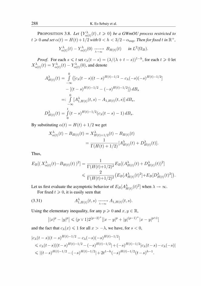
PROPOSITION 3.8. Let Y λα(t)(t) , t 0 be a GWmOU process restricted to
t 0 and set α(t) = H(t)+1/2 with 0 < h < 3/2−αsup. Then for fixed t in R+,
Y λα(t)(t)− Y
λα(t)(0) −−−→
λ→∞BH(t)(t) in L2(ΩB).
Proof. For each s ¬ t set cλ(t − s) = (λ/(λ + t − s))1−h, for each t 0 letXλα(t)(t) = Y λ
α(t)(t)− Yλα(t)(0), and denote
AλH(t)(t) =0∫−∞
([cλ(t− s)(t− s)H(t)−1/2 − cλ(−s)(−s)H(t)−1/2]
− [(t− s)H(t)−1/2 − (−s)H(t)−1/2])dBs
=:0∫−∞
[Aλ1,H(t)(t, s)−A1,H(t)(t, s)] dBs,
DλH(t)(t) =
t∫0
(t− s)H(t)−1/2(cλ(t− s)− 1) dBs.
By substituting α(t) = H(t) + 1/2 we get
Xλα(t)(t)−BH(t)(t) = Xλ
H(t)+1/2(t)−BH(t)(t)
=1
Γ(H(t) + 1/2)[AλH(t)(t) +Dλ
H(t)(t)].
Thus,
EB[(Xλα(t)(t)−BH(t)(t) )2] =
1
Γ(H(t)+1/2)2EB[(AλH(t)(t) +Dλ
H(t)(t))2]
¬ 2
Γ(H(t)+1/2)2
(EB[AλH(t)(t)
2]+EB[DλH(t)(t)
2]).
Let us first evaluate the asymptotic behavior of EB[AλH(t)(t)2] when λ→∞.
For fixed t 0, it is easily seen that
(3.31) Aλ1,H(t)(t, s) −−−→λ→∞A1,H(t)(t, s).
Using the elementary inequality, for any p 0 and x, y ∈ R,∣∣|x|p − |y|p∣∣ ¬ (p ∨ 1)2(p−2)+ [|x− y|p + |y|(p−1)+ |x− y|p∧1]
and the fact that cλ(x) ¬ 1 for all x > −λ, we have, for s < 0,
|cλ(t− s)(t− s)H(t)−1/2 − cλ(−s)(−s)H(t)−1/2|¬ cλ(t−s)|(t−s)H(t)−1/2−(−s)H(t)−1/2|+(−s)H(t)−1/2|cλ(t−s)−cλ(−s)|¬ |(t−s)H(t)−1/2−(−s)H(t)−1/2|+2t1−h(−s)H(t)−1/2(t−s)h−1.
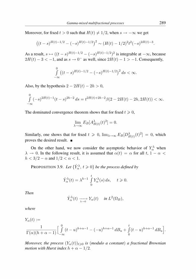
Gamma-mixed multifractional processes 289
Moreover, for fixed t > 0 such that H(t) 6= 1/2, when s→ −∞ we get((t− s)H(t)−1/2 − (−s)H(t)−1/2
)2 ∼ (H(t)− 1/2)2t2(−s)2H(t)−3.
As a result, s 7→ ((t− s)H(t)−1/2 − (−s)H(t)−1/2)2 is integrable at −∞, because2H(t)− 3 < −1, and as s→ 0− as well, since 2H(t)− 1 > −1. Consequently,
0∫−∞
((t− s)H(t)−1/2 − (−s)H(t)−1/2
)2ds <∞.
Also, by the hypothesis 2− 2H(t)− 2h > 0,
0∫−∞
(−s)2H(t)−1(t− s)2h−2 ds = t2H(t)+2h−2β(2− 2H(t)− 2h, 2H(t)) <∞.
The dominated convergence theorem shows that for fixed t 0,
limλ→∞
EB[AλH(t)(t)2] = 0.
Similarly, one shows that for fixed t 0, limλ→∞EB[DλH(t)(t)
2] = 0, whichproves the desired result.
On the other hand, we now consider the asymptotic behavior of Y λα when
λ → 0. In the following result, it is assumed that α(t) = α for all t, 1 − α <h < 3/2− α and 1/2 < α < 1.
PROPOSITION 3.9. Let Y λα , t 0 be the process defined by
Y λα (t) = λh−1
t∫0
Y λα (s) ds, t 0.
ThenY λα (t) −−→
λ→0Yα(t) in L2(ΩB),
where
Yα(t) :=
1
Γ(α)(h+ α− 1)
[ 0∫−∞
(t− u)h+α−1 − (−u)h+α−1 dBu +t∫0
(t− u)h+α−1 dBu
].
Moreover, the process (Yα(t))t0 is (modulo a constant) a fractional Brownianmotion with Hurst index h+ α− 1/2.

290 K. Es-Sebaiy et al.
Proof. For each t 0, we have
λh−1t∫0
Y λα (s) ds =
1
Γ(α)
t∫−∞
dBut∫
u∨0
(λ+ s− u)h−1(s− u)α−1 ds
=1
Γ(α)
0∫−∞
dBut∫0
(λ+ s− u)h−1(s− u)α−1 ds
+1
Γ(α)
t∫0
dBut∫u
(λ+ s− u)h−1(s− u)α−1 ds.
Using the same computations as in the proof of Proposition 3.8, it is easily checkedthat for every t 0,
Y λα (t) −−→
λ→0Yα(t) :=
1
Γ(α)(h+ α− 1)
[ 0∫−∞
(t− u)h+α−1 − (−u)h+α−1 dBu +t∫0
(t− u)h+α−1 dBu
]in L2(ΩB). Moreover, it is obvious that the process (Yα(t))t0 is (modulo a con-stant) a fractional Brownian motion (with moving average definition) with Hurstindex h+ α− 1/2.
4. APPENDIX
PROPOSITION 4.1. For all 0 < p < 1 and k 2,
(4.1)k∑i=1
xpi ¬ 2(k−1)(1−p)( k∑i=1
xi
)pif xi 0 for i = 1, . . . , k.
Proof. For k 2, 0 < p < 1 and xi 0 for all i = 1, . . . , k, we will denoteby A(k) the inequality
A(k) :k∑i=1
xpi ¬ 2(k−1)(1−p)( k∑i=1
xi
)p.
Let k = 2. Since the function x 7→ xp, x 0, is concave for every 0 < p < 1, weget
xp + yp ¬ 21−p(x+ y)p,
so A(2) holds true.Let us assume thatA(n−1) holds. UsingA(2),A(n−1), by easy computations
we get A(n). Thus by induction, the proof is complete.

Gamma-mixed multifractional processes 291
Throughout the appendix, it is supposed that 0 < h < 3/2−Mα[a, b],Mα[a, b]< 1 and mα[a, b] > 1/2 for any compact interval [a, b] ⊂ R.
LEMMA 4.1. Fix a compact interval [a, b] ⊂ R. There exists a constant Cdepending only on [a, b], λ and h such that
EB[(Y λα(t)(t+ τ)− Y λ
α(t)(t))2] ¬ C|τ |2α(t)−1
for all t, t+ τ ∈ [a, b] with |τ | < 1.
Proof. Set η = 3 − 2h − 2α(t), ν = 2α(t) − 1 and y = |τ |/λ. Using (3.21),we get
(4.2) EB[(Y λα(t)(t+ τ)− Y λ
α(t)(t))2]
= EB[(Y λα(t)(t+ τ))2] + EB[Y λ
α(t)(t)2]− 2EB[Y λ
α(t)(t+ τ)Y λα(t)(t)]
=2λν
Γ(α(t))2β(η, ν)− 2EB[Y λ
α(t)(t+ τ)Y λα(t)(t)].
Let us first evaluate the second term on the right hand side. By (3.22) we have
(4.3) −2EB[Y λα(t)(t+ τ)Y λ
α(t)(t)]
=−2λν
Γ(α(t))2
1∫0
uη−1(1− u)α(t)−1(1 + yu)h−1(yu+ 1− u)α(t)−1 du.
By applying the mean value theorem to the function t 7→ (1+yt)h−1 for t ∈ [0, u],we obtain
(4.4) −2EB[Y λα(t)(t+ τ)Y λ
α(t)(t)]
=−2λν
Γ(α(t))2
1∫0
uη−1(1− u)ν−1
(1 + y
u
1− u
)α(t)−1
du
+2λν(1− h)
Γ(α(t))2y
1∫0
(1 + yCu)h−2uη (1− u)α(t)−1(yu+ 1− u)α(t)−1 du
=: Aλ,h(α(t), y) +Bλ,h(α(t), y).
Let us begin by providing an upper bound for Aλ,h. Using the inequality
1− yu
1− (1− y)u¬(
1 + yu
1− u
)α(t)−1
,
292 K. Es-Sebaiy et al.
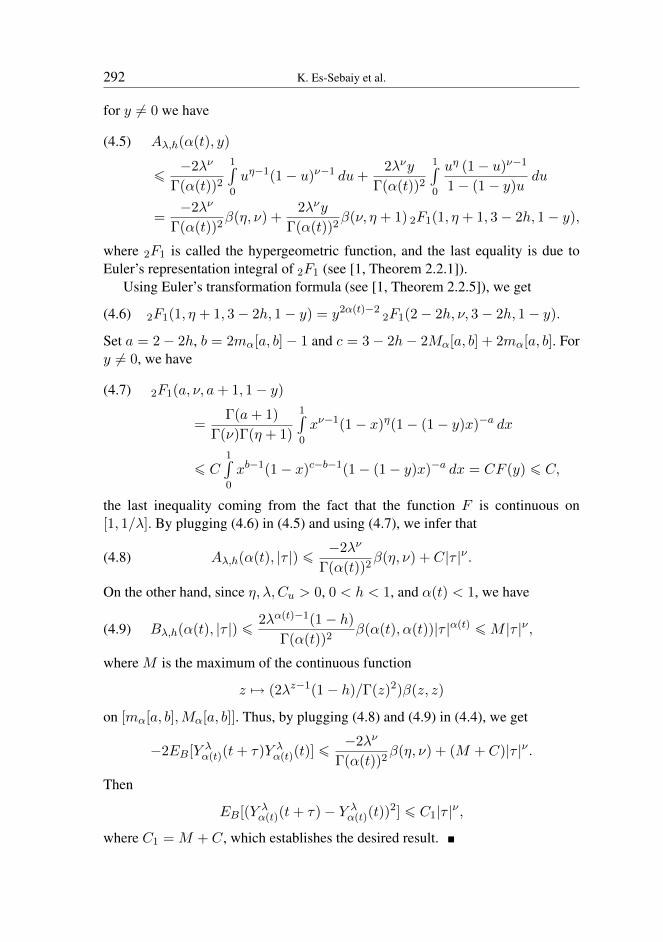
for y 6= 0 we have
(4.5) Aλ,h(α(t), y)
¬ −2λν
Γ(α(t))2
1∫0
uη−1(1− u)ν−1 du+2λνy
Γ(α(t))2
1∫0
uη (1− u)ν−1
1− (1− y)udu
=−2λν
Γ(α(t))2β(η, ν) +
2λνy
Γ(α(t))2β(ν, η + 1) 2F1(1, η + 1, 3− 2h, 1− y),
where 2F1 is called the hypergeometric function, and the last equality is due toEuler’s representation integral of 2F1 (see [1, Theorem 2.2.1]).
Using Euler’s transformation formula (see [1, Theorem 2.2.5]), we get
(4.6) 2F1(1, η + 1, 3− 2h, 1− y) = y2α(t)−22F1(2− 2h, ν, 3− 2h, 1− y).
Set a = 2− 2h, b = 2mα[a, b]− 1 and c = 3− 2h− 2Mα[a, b] + 2mα[a, b]. Fory 6= 0, we have
(4.7) 2F1(a, ν, a+ 1, 1− y)
=Γ(a+ 1)
Γ(ν)Γ(η + 1)
1∫0
xν−1(1− x)η(1− (1− y)x)−a dx
¬ C1∫0
xb−1(1− x)c−b−1(1− (1− y)x)−a dx = CF (y) ¬ C,
the last inequality coming from the fact that the function F is continuous on[1, 1/λ]. By plugging (4.6) in (4.5) and using (4.7), we infer that
Aλ,h(α(t), |τ |) ¬ −2λν
Γ(α(t))2β(η, ν) + C|τ |ν .(4.8)
On the other hand, since η, λ, Cu > 0, 0 < h < 1, and α(t) < 1, we have
Bλ,h(α(t), |τ |) ¬ 2λα(t)−1(1− h)
Γ(α(t))2β(α(t), α(t))|τ |α(t) ¬M |τ |ν ,(4.9)
where M is the maximum of the continuous function
z 7→ (2λz−1(1− h)/Γ(z)2)β(z, z)
on [mα[a, b],Mα[a, b]]. Thus, by plugging (4.8) and (4.9) in (4.4), we get
−2EB[Y λα(t)(t+ τ)Y λ
α(t)(t)] ¬−2λν
Γ(α(t))2β(η, ν) + (M + C)|τ |ν .
Then
EB[(Y λα(t)(t+ τ)− Y λ
α(t)(t))2] ¬ C1|τ |ν ,
where C1 = M + C, which establishes the desired result.

Gamma-mixed multifractional processes 293
LEMMA 4.2. Fix a compact interval [a, b] ⊂ R.
(1) There exists a constant C2 depending only on [a, b], λ and h such that
(4.10) EB[(Y λα(t)(t+ τ)− Y λ
α(t)(t))2] C2|τ |2α(t)−1
for all t, t+ τ ∈ [a, b] with |τ | < 1.
(2) As τ → 0,
(4.11) EB[(Y λα(t)(t+ τ)− Y λ
α(t)(t))2] = C2|τ |α(t)−1/2 +O(|τ |2α(t)−1).
Proof. With the notation of Lemma 4.1, since α(t) < 1 for all t, we have
Bλ,h(α(t), y) ¬ EB[(Y λα(t)(t+ τ)− Y λ
α(t)(t))2].
For τ 6= 0, using Cu ∈ ]0, 1[ we get(1
|τ |+
1
λ
)α(t)+h−3
|τ |2α(t)−2 ¬ (1 + y)h+α(t)−3(4.12)
¬ (1− u+ yu)α(t)−1(1 + yCu)h−2.
Seth(z, x) = (λx)3−z−h(x+ λ)z+h−3,
a continuous function on [mα[a, b],Mα[a, b]] × [0, 1], and let C2 be the minimumof the function
(z, x) 7→ 2λ2z−2(1− h)
Γ(z)2β(4− 2h− 2z, z)h(z, x)
for (z, x) ∈ [mα[a, b],Mα[a, b]]× [0, 1]. Then
EB[(Y λα(t)(t+ τ)− Y λ
α(t)(t))2] C2|τ |ν ,
which gives (4.10).Let us now prove (4.11). If instead of (4.12) we use the following inequality for
y 6= 0: (1
|τ |+
1
λ
)α(t)+h−3
|τ |α(t)−3/2 ¬ (1 + y)α(t)+h−3,
then (4.10) becomes
EB[(Y λα(t)(t+ τ)− Y λ
α(t)(t))2] C2|τ |α(t)−1/2.

294 K. Es-Sebaiy et al.
Combining Lemma 4.1 and the last inequality, we get
C2|τ |α(t)−1/2 ¬ EB[(Y λα(t)(t+ τ)− Y λ
α(t)(t))2] ¬ C1|τ |α(t)−1/2.
To prove (4.11), it remains to show thatC2 ¬ C1 = M+C. Since 0 < h < 3/2−zand z < 1, we obtain
β(4− 2h− 2z, z) ¬ β(z, z) and h(z, x) ¬ λ1−z.
Therefore,
C2 ¬2λ2z−2(1− h)
Γ(z)2β(4− 2h− 2z, z)h(z, x) ¬M ¬ C1,
which completes the proof.
REFERENCES
[1] G. Andrews, R. Askey and R. Roy, Special Functions, Cambridge Univ. Press, 1999.[2] A. Ayache, S. Jaffard and M. S. Taqqu, Wavelet construction of generalized multifractional
processes, Rev. Mat. Iberoamer. 23 (2007), 327–370.[3] A. Ayache and M. S. Taqqu, Multifractional processes with random exponent, Publ. Mat. 49
(2005), 459–486.[4] A. Benassi, S. Jaffard and D. Roux, Elliptic Gaussian random processes, Rev. Mat. Iberoamer.
13 (1997), 19–90.[5] S. Bianchi, Pathwise identification of the memory function of multifractional Brownian motion
with application to finance, Int. J. Theoret. Appl. Finance 8 (2005), 255–281.[6] P. Billingsley, Convergence of Probability Measures, Wiley, New York, 1968.[7] P. Billingsley, Convergence of Probability Measures, 2nd ed., Wiley, New York, 1999.[8] P. Cheridito, H. Kawaguchi and M. Maejima, Fractional Ornstein–Uhlenbeck processes, Elec-
tron. J. Probab. 8 (2003), no. 3, 14 pp.[9] S. Eryilmaz, δ-shock model based on Polya process and its optimal replacement policy, Eur. J.
Oper. Res. 263 (2017), 690–697.[10] K. Es-Sebaiy and C. A. Tudor, Fractional Ornstein–Uhlenbeck processes mixed with a Gamma
distribution, Fractals 23 (2015), no. 3, art. 1550032, 10 pp.[11] K. Falconer, Fractal Geometry. Mathematical Foundations and Applications, 2nd ed., Wiley,
2003.[12] P. Flandrin, P. Borgnat and P. O. Amblard, From stationarity to self-similarity, and back: Vari-
ations on the Lamperti transformation, in: Processes with Long-Range Correlations, LectureNotes in Phys. 621, Springer, New York, 2003, 88–117.
[13] E. Iglói and G. Terdik, Long-range dependence through Gamma-mixed Ornstein–Uhlenbeckprocess, Electron. J. Probab. 4 (1999), no. 16, 33 pp.
[14] S. C. Lim and C. H. Eab, Riemann–Liouville and Weyl fractional oscillator processes, Phys.Lett. A 355 (2006), 87–93.
[15] S. C. Lim and L. P. Teo, Weyl and Riemann–Liouville multifractional Ornstein–Uhlenbeckprocesses, J. Phys. A 40 (2007), 6035–6060.
[16] K. S. Miller and B. Ross, An Introduction to the Fractional Calculus and Fractional DifferentialEquations, Wiley, New York, 1993.
[17] R. F. Peltier and J. Lévy Véhel, Multifractional Brownian motion: definition and preliminaryresults, Research Report RR-2645, INRIA, 1995.

Gamma-mixed multifractional processes 295
[18] S. Samko, A. A. Kilbas and D. I. Marichev, Fractional Integrals and Derivatives. Theory andApplications, Gordon and Breach, Amsterdam, 1993.
[19] S. Stoev and M. S. Taqqu, How rich is the class of multifractional Brownian motions?, Stoch.Process. Appl. 116 (2006), 200–221.
Khalifa Es-SebaiyDepartment of MathematicsFaculty of ScienceKuwait UniversityP.O. Box 5969Safat 13060, KuwaitE-mail: [email protected]
Fatima-Ezzahra FarahDepartment of Mathematics
National School of Applied Sciences, MarrakeshCadi Ayyad University
BP GuélizBoulevard Abdelkrim Al Khattabi
Marrakesh, MoroccoE-mail: [email protected]
Astrid HilbertDepartment of MathematicsFaculty of TechnologyLinnaeus UniversityP G Vejdes väg351 95 Växjö, SwedenE-mail: [email protected]
Received 21.3.2019;revised version 12.6.2019
