1

WESTERN GRAY WHALE ADVISORY PANEL WGWAP:

4-D Seismic Survey Task Force

2nd meeting of the task force

13 – 16 March 2008

Lausanne, Switzerland

REPORT OF THE TASK FORCE

CONVENED BY IUCN

2

Table of contents

1 INTRODUCTORY ITEMS ...............................................................................................................4 1.1 CHAIR’S OPENING REMARKS AND GENERAL SUMMARY OF EARLIER DISCUSSIONS ...................................... 4 1.2 ARRANGEMENTS FOR THE WORKSHOP ....................................................................................................... 4 1.3 APPOINTMENT OF RAPPORTEURS................................................................................................................ 4 1.4 ADOPTION OF AGENDA............................................................................................................................... 5 1.5 AVAILABLE DOCUMENTS ............................................................................................................................ 5 2 SURVEY PLANS AND DEADLINES..............................................................................................5 2.1 SURVEY PREPARATION TIMING ................................................................................................................... 6 2.2 SURVEY DESIGN SPECIFICS.......................................................................................................................... 6 3 REVIEW OF WHITE PAPER ON SEISMIC SURVEY METHODS ..........................................8 3.1 SUMMARY OF ‘WHITE PAPER’ ..................................................................................................................... 8

3.1.1 SEIC’s evaluation of the feasibility of ice-based surveys offshore Sakhalin .................................... 9 3.1.2 SEIC’s Astokh 4D Source Optimisation Project............................................................................... 9

3.2 DISCUSSION (INCL. RESULTS OF INDEPENDENT REVIEW)........................................................................... 10 3.3 IMPLICATIONS FOR FUTURE SESIMIC SURVEY(S) ....................................................................................... 11 4 REVIEW OF WGW DENSITY DATA AND THEIR USE IN ASSESSING POTENTIAL

IMPACTS OF THE SEISMIC SURVEY .....................................................................12 4.1 WESTERN GRAY WHALE DENSITY ANALYSIS............................................................................................. 12 4.2 FROM DENSITY TO NUMBERS .................................................................................................................... 15 5 REVIEW OF RESULTS/PROGRESS ON ACOUSTIC MODELLING EXERCISES ............15 5.1 DATA ISSUES............................................................................................................................................. 15 5.2 METHODS ................................................................................................................................................. 15

5.2.1 SEIC Team...................................................................................................................................... 16 5.2.2 Russian Team ................................................................................................................................. 19

5.2.2.1 Input data....................................................................................................................................................20 5.2.2.2 The methodology........................................................................................................................................20

5.2.3 Conclusions and recommendations ................................................................................................ 21 5.3 VALIDATION OF MODELLING RESULTS ...................................................................................................... 21

5.3.1 Comparison with 2001 data ........................................................................................................... 22 5.3.2 Comparison with 1997 data ........................................................................................................... 26

5.4 RESULTS ................................................................................................................................................... 26 5.4.1 SEIC Team...................................................................................................................................... 26

5.5 REAL-TIME CALIBRATION ISSUES (COMPARISON OF MODELLING RESULTS WITH REAL-TIME MEASUREMENTS) ...................................................................................................................................... 28

6 FURTHER CONSIDERATION OF THE DOSE-BASED APPROACH....................................30 6.1 LITERATURE REVIEW ................................................................................................................................ 30 6.2 DISCUSSION AND IMPLICATIONS/RECOMMENDATIONS FOR FORTHCOMING SURVEY ................................. 31 7 MITIGATION AND MONITORING ............................................................................................32 7.1 SUMMARY OF EXISTING MITIGATION MEASURES....................................................................................... 32 7.2 OBJECTIVES .............................................................................................................................................. 32 7.3 BACKGROUND INFORMATION ................................................................................................................... 33

7.3.1 Estimation of detection function of MMOs..................................................................................... 33 7.3.2 Technical issues surrounding real-time acoustic monitoring......................................................... 34

7.4 EXAMINATION OF RISK ............................................................................................................................. 34 7.4.1 Use of whale density data to delineate the feeding area and assess potential impacts of the 2009

SEIC seismic survey ....................................................................................................................... 34 7.4.1.1 Proposed Piltun feeding area perimeter monitoring line.............................................................................34 7.4.1.2 Use of the density data to assess potential impacts from the 2009 survey..................................................35

7.4.2 Estimation of effectiveness of mitigation measures ........................................................................ 37

3

7.5 MONITORING (NUMBER, DISTRIBUTION, BEHAVIOUR)............................................................................... 38 7.5.1 Acoustic monitoring (perimeter and within area) .......................................................................... 39

7.5.1.1 Along the perimeter of the feeding area .....................................................................................................39 7.5.1.2 Within the feeding area ..............................................................................................................................39

7.5.2 General visual monitoring (shore-based and vessel-based)........................................................... 39 7.5.2.1 Within the feeding area (shore-based)........................................................................................................39 7.5.2.2 Within the feeding area (vessel-based).......................................................................................................40 7.5.2.3 Within the proximity of the seismic related vessel(s).................................................................................40

7.6 MITIGATION MEASURES............................................................................................................................ 41 7.6.1 Timing of surveys............................................................................................................................ 41 7.6.2 General design and conduct of surveys .......................................................................................... 41

7.6.2.1 Definition and updating of A and B zones .................................................................................................41 7.6.2.2 Measures within the proximity of the seismic vessel – entire survey .........................................................41 7.6.2.3 Additional restrictions for Zone A..............................................................................................................42

8 CONCLUSIONS...............................................................................................................................42 9 ADOPTION OF THE REPORT .....................................................................................................43 REFERENCES......................................................................................................................................44 ANNEX A - AGENDA..........................................................................................................................46 ANNEX B - LIST OF DOCUMENTS.................................................................................................48 ANNEX C - TERMS OF REFERENCE FOR THE ASTOKH 4D SEISMIC TASK FORCE .....49 ANNEX D - COMPARISON PLOTS BETWEEN 2001 ENL SURVEY ACOUSTIC

MEASUREMENTS AND MODEL PREDICTIONS ..................................................52 ANNEX E - ILLUSTRATIVE CALCULATIONS OF EFFECTIVENESS OF SHUTDOWN

CRITERIA FOR REDUCING SOUND EXPOSURE RISK ......................................55

4

Members: Justin Cooke, Greg Donovan (Chair), Doug Nowacek, Alexander Vedenev, Judy Muir, Glenn Gailey, Mark Downes, Roberto Racca, Matthew Angelatos, Doug Bell, Ingrid Rosenberger, Sarah Gotheil.

1 INTRODUCTORY ITEMS

1.1 Chair’s opening remarks and general summary of earlier discussions The Chair welcomed the participants to the Workshop. He stressed that the intention was not to reopen all previous discussions but rather to build upon the work undertaken at the workshop held in The Hague from 25-28 June 2007 (WGWAP 3/INF.9) and the subsequent discussions at the WGWAP-3 meeting.

At WGWAP-3, SEIC had indicated that for safety reasons (see Item 2.1) the seismic work originally planned for 2008 was to be postponed until 2009. This postponement had the advantage that it meant that matters raised by the Task Force but not addressed thoroughly because of time constraints could be examined in greater depth. The Panel, whilst agreeing with the overall approach and mitigation measures recommended by the Task Force, had agreed that further work was required inter alia on the quantitative aspects of the work, especially those related to threshold levels. In summary, the Panel had agreed that the following items merited further discussion: whether to use a dose-based approach; the threshold levels themselves; estimation of doses received; effectiveness of the proposed mitigation measures; estimation of transmission loss and calibration of model predictions; adequacy and reliability of sound monitoring equipment; and monitoring of possible whale responses. It agreed that the best way to address these issues was by continuation of the Task Force, and to this end, detailed Terms of Reference and a work plan were developed. These are given as Annex C to this report.

The Chair also reminded the participants of the need to respect the confidentiality agreement given at the end of the Terms of Reference. One of the primary benefits of the Task Force approach was to encourage data sharing and collaborative analyses to enable the best scientific advice to be provided. This works best via a combination of respect for data owners and a level of informality. In terms of the report itself, it was agreed that the report should contain data only at the level required to justify the conclusions. It was also recognised that the report of the Task Force, once finalised and presented at WGWAP-4, would become a public, unalterable document. It is up to the Panel itself to decide whether or not it agrees with some or all of the recommendations therein.

He noted that the aim was to arrive at a consensus report that could be read as a stand-alone document, although referencing the previous workshop report (WGWAP 3/INF.9). Where appropriate, a summary or details from the previous workshop have been incorporated into the present report.

1.2 Arrangements for the Workshop Gotheil introduced the working arrangements for the Workshop.

1.3 Appointment of Rapporteurs Gotheil took notes of all discussions. A number of participants contributed to the final report. Final editing was carried out by the Chair.

5

1.4 Adoption of Agenda The Chair explained that the primary purpose of the Agenda was to try to ensure that all major topics were covered and to provide a structure for the discussions and the report. He noted that not all of the items would necessarily be discussed in the precise order of the agreed agenda depending on circumstances and the need to undertake analyses at the meeting. There was also a degree of interaction between some agenda items. The agreed Agenda is given as Annex A.

1.5 Available documents The list of available documents is given as Annex C.

2 SURVEY PLANS AND DEADLINES SEIC provided the following summary of the seismic survey plans (this incorporates details originally presented in WGWAP 3/INF.9.

The Piltun-Astokh (PA) field was discovered in 1986 ca 12-15km offshore at water depths between 30 and 50m. Since then, 17 exploration and appraisal wells have been drilled, of which four reside in the producing Astokh area. The Astokh portion of this field began production from the PA-A (Molikpaq) platform in 1999. Between 1999 and 2001, 13 production wells were drilled and brought on line. Production has been seasonal thus far, but with the planned hook-up to the pipeline there will be year-round production.

In 2003-2005, the pressure-maintenance project was carried out, entailing the drilling of four dedicated water-injection wells on the periphery of the field. This project was undertaken to increase reservoir pressure and enhance recovery by water drive. The fourth injection well was brought on line in April 2005. In 2006, pressures were restored to levels close to original. The location of the injection-related waterfront is unknown, and no water-breakthrough has occurred in production wells to date.

The Astokh Further Development project will entail infill drilling from the existing Molikpaq platform to increase the recovery from the field and meet levels of recovery that are commitments to the Russian Authorities. The complex reservoirs at Astokh, however, mean that efficient development of this large resource cannot be undertaken without monitoring the area changes in water and oil movement across the structure. The availability of a seismic-based map of reservoir changes will allow recovery commitments to be met with fewer production wells. These additional wells will be drilled from the Molikpaq.

At Astokh, efficient recovery of oil and gas from this large reservoir is dependent upon reliable information regarding production-related spatial pressure and fluid changes in the reservoir and surrounding formations. Such information enables a given recovery fraction to be achieved with fewer wells, thus potentially reducing the risk to the environment.

As discussed under Item 3 below, an evaluation by SEIC of all available techniques for spatial field monitoring concluded that unproven, non-conventional methods (e.g. Time Lapse Electromagnetics and Gravity) will not yield the horizontal and vertical resolution required to image production-related effects within the Astokh reservoir. In 1997, the full PA license area was surveyed with a 3D seismic system. This ‘baseline survey’ was acquired by the PGS vessel Nordic Explore between the months of July and August. These data, reanalysed in 2001 resulting in a higher quality ‘stack’, are deemed suitable by SEIC as a base survey for reservoir

monitoring purposes. The Astokh Field has been under production for several seasons, and thus SEIC consider that a repeat of the original 3D streamer seismic survey to be the only technically feasible time-lapse method that can be used to prevent the drilling of unnecessary wells.

The technical feasibility of imaging production-related changes at Astokh has been assessed using a forward modelling approach. These models indicate that acoustically subtle production-related changes can be imaged. However, during a repeat 3D survey (often called a 4D survey in the industry, where the fourth dimension is time), the original pre-production survey design and acquisition specifics, particularly source size and array geometry and source-to-receiver positioning, will need to be matched as closely as possible with those of the 1997 survey.

2.1 Survey preparation timing SEIC is preparing to undertake the survey during the summer of 2009. As noted above, this represents a one-year delay from the original plan due to safety concerns around the presence of production vessels near the Molikpaq. Further delay is not envisaged.

SEIC is preparing to tender for the 2009 survey. As the most effective mitigation measure is to ensure that the survey is completed prior to the peak WGW migration period, SEIC plans to commence the tendering exercise before July 2008. This timeframe will (1) improve the likelihood of sourcing the required vessel specification in the remote Sakhalin location and (2) reduce the risk of delays due to interference from potential simultaneous seismic operations (e.g. Regional 2D seismic surveys by other operators).

SEIC noted that it values the WGWAP advice and recommendations and considers it imperative that the mitigation and monitoring plans are finalised in April 2008 for inclusion in the draft EIA. This draft EIA material is required to be submitted with the survey tender documentation.

Figure 2.1 - Timescale for the 2009 SEIC seismic survey.

2.2 Survey design specifics Production-related effects in the reservoir are acoustically subtle. Therefore, to measure changes over time, the original 1997 survey must be repeated exactly i.e. the source-to-receiver position and source level must be identical. Although the source level requirement has been and is being investigated vis-à-vis reducing the exposure of gray whales to noise in future surveys, SEIC does not consider that such a reduction is an option for the proposed 2009 survey. To ensure consistency between the 1997 and 2009 surveys, baseline orientations and acquisition directions must be repeated exactly. There is, however, no requirement to re-acquire the full area of the original data: the repeat survey has been limited to areas where the production-related effects are expected.

6

Astokh 2009 Repeat Seismic Survey

Figure 2.2 - Map of Astokh 2009 survey shot area with coastline and bathymetry shown.

7

8

The key parameters of the original 1997 survey are indicated below:

(1) Mode • 6 Streamers /dual source • Shot interval – 18.75m (flip-flop), corresponding to approximately 7.2 seconds between

pulses during normal survey at 5 knots

(2) Receivers/cables • 4500m long, 100m separation and 8m depth

(3) Source • 2 x 2620 cu in sleeve arrays • 3 sub-arrays with 10m separation • Depth 6m • Length 14m • 2000 psi firing pressure.

As noted above, a significant element of impact mitigation is the reduction of the survey area to 90 km2 - <20% of the 1997 design. This has been achieved by limiting it to the sector of the field where production-related effects are expected. To acquire seismic data and image the area of interest, the actual 1997 line orientation and source-to-receiver position will have to be replicated exactly. This will require acquisition of an area of approximately 170km2 (Fig. 2.2). A seam exists in the 1997 data at the boundary between N-S and S-N lines. The lines are spaced approximately 300m apart. It is expected that the array will be towed about 220m behind the vessel.

SEIC predict that to acquire the necessary data, the vessel will be active for approximately 21 days. The actual duration of the survey (and the durations of impact) will be dependent upon the final mitigation measures that are implemented by SEIC, and the survey standby time that results from those as well as other factors (e.g. poor weather) . However, of these 3+ weeks, it is estimated that approximately only 4-5 days of actual seismic source activity will be required. This period of fully active pulsed seismic source will be non-continuous and interspersed with frequent intervals of reduced activity (such as during line changes) or complete inactivity (vessel downtime during rigging-up, poor weather conditions or nearby gray whales).

At least three vessels are likely to be involved with the acquisition – a master seismic vessel, a guard vessel and a supply vessel. The guard vessel follows the streamers to ensure that they are deployed properly and not compromised by other vessels.

3 REVIEW OF WHITE PAPER ON SEISMIC SURVEY METHODS

3.1 Summary of ‘white paper’

At WGWAP-3, some time was spent discussing the possibility of conducting the 2009 survey using lower sound volumes. While not averse to changes in methods per se, SEIC reiterated the need to obtain results that are comparable to those of the 1997 survey; changes that do not allow this objective to be met render the survey worthless. Given the importance of this topic, SEIC offered to develop a technical ‘white paper’ presenting its view of potential alternatives to a

9

straight repeat of the 1997 survey (and see Annex C). This review (Seismic TF 2/Doc.3) was circulated in advance. SEIC’s summary of the main points in the white paper is given below.

3.1.1 SEIC’s evaluation of the feasibility of ice-based surveys offshore Sakhalin One idea that has been raised is the option of acquiring a new baseline survey (for time-lapse imaging of the Astokh reservoir) and future repeats that would be conducted during periods when western gray whales are absent (i.e. in winter), therefore reducing direct impacts on them.

As noted in Seismic TF 2/Doc.3, winter ice conditions in the vicinity of Piltun and Astokh are complex, variable and markedly different from those in areas of land-fast ice where trials of winter seismic acquisition have been undertaken (e.g. Alaska). Conditions typically entail a thin strip of ridged landfast ice along shore and extending up to 8km seaward, often bounded by a coastal flaw lead or polynya of open water or thin, very mobile ice, typically 6-18km wide, beyond which there is commonly mobile offshore pack-ice with thick keels 10-15m and sometimes up to 20-25m deep.

The Workshop agreed that at present there are no technically proven options for acquiring reliable seismic data in the ice conditions encountered over Piltun Astokh during the winter months. Of the potential techniques examined, the use of ocean bottom receivers offers the greatest potential for technical success although this approach is frequently not commercially feasible under benign open water conditions. This approach faces several additional technical and environmental problems and is yet to be tested in Arctic conditions.

The Workshop was informed that to further explore the feasibility of winter acquisition, SEIC has initiated and is co-funding a long-term research programme with the Shell Arctic Research Group. The short-term aim of this programme, in conjunction with the Shell Alaskan Group, is a detailed assessment of existing vendor technologies. After this initial feasibility stage, it is hoped that one or more field trials could be conducted offshore Sakhalin with the aim of being ready for implementation by 2011 at the earliest. Clearly, achieving this goal will depend on the success of interim steps.

In conclusion, the Workshop agreed that surveys in winter, when no whales are present, are a very desirable option. However, it recognised that it is too early to assess the prospects for development of a winter survey method. It looks forward to receiving the reports of the development work.

3.1.2 SEIC’s Astokh 4D Source Optimisation Project At the request of the WGWAP, SEIC investigated options with the potential to reduce the environmental impact of the proposed 2009 Astokh 4D survey airgun array, primarily by reducing acoustic levels in the adjacent feeding area.

The principal limitation in the ability to reduce source levels during acquisition is the very subtle production-related effects that are expected in the target reservoirs. The 2009 seismic survey results are essential for specifying the subsequent drilling work and thus failure to obtain data of adequate quality is considered unacceptable by SEIC. Furthermore, failure may result in the need for re-acquisition with the additional disturbance this may entail; if it had to be in late 2009, larger numbers of gray whales are likely to be present.

As noted in Seismic TF 2/Doc.3, direct reduction of source energy (compared to 1997 levels) is not considered feasible for the 2009 survey. In addition to technical concerns, the option of fold-

10

compensation by increasing the number of shots poses negative environmental repercussions in terms of both survey duration and possibly cumulative received levels within the feeding area. However, Seismic TF 2/Doc.3 did identify the possibility of using additional streamers to compensate for reduced source levels; this may also yield benefits to survey repeatability. The major problem is logistical i.e. the ability of SEIC to secure a vessel with the capability to tow the additional streamers. Vessel contractors may also have limitations in the number of towed streamers based on the shallow water depths in the Astokh area. The remote location of Sakhalin and the tight global vessel market are contributing factors and a clearer indication of the feasibility of this approach will only be known after competitive tendering has occurred.

The Workshop agreed that every effort should be made to obtain a suitable vessel.

In addition, acoustic modelling predictions at Astokh indicate that the inshore propagation of sound contours is dominated by high frequencies (100Hz+). This end of the spectrum is not required for subsurface imaging (but is probably well within the hearing range of gray whales) and the Workshop welcomed the information that an SEIC research project has been initiated to investigate the potential for avoiding the generation of these frequencies at the source array.

3.2 Discussion (incl. results of independent review) As noted in Annex C, it had been agreed that the Task Force would also have the benefit of an independent review of Seismic TF 2/Doc.3. This was undertaken by Dr. John Diebold from the Lamont-Doherty Earth Observatory at Columbia University in New York, USA (Seismic TF 2/Doc. 4). In summary, Diebold agreed that SEIC had given serious consideration to attempts to reduce the size of the seismic array they propose to use for the 2009 Astokh surveys and he broadly agreed with the conclusions of Seismic TF 2/Doc. 3.

Diebold provided a simple explanation as to why ‘tuning’ of the array is important and, moreover, why the combination of airguns proposed for use by SEIC is important in attaining this tuning. After reviewing SEIC’s examination of the possibility of constructing an array with appropriate characteristics to allow comparable results with the 1997 survey but using only half the peak output of the original array, Diebold concurred with SEIC’s overall conclusion that reducing the source array substantially will not be effective. This is primarily due to the occurrence of so-called incoherent noise, for which there is no way to compensate even in post processing, i.e., the incoherent noise would compromise the signal:noise ratio (S/N) necessary to achieve the goals of the survey.

While concurring with the SEIC conclusion, Diebold did note, however, that the assumption in Seismic TF 2/Doc. 3 that all incoherent noise is ambient was somewhat naïve. SEIC had considered the idea of adding receivers in order to achieve the desired S/N, but stated that it was not logistically feasible to add enough hydrophones (‘streamers’) to compensate for reducing the source array by as much as half. Other methods considered by SEIC included the use of vibrator source or the use of a different type of airgun; Diebold concurred with the view that at this stage, neither represents a viable way to reduce the source volume. Finally, Diebold suggested that other ameliorative approaches could be considered, specifically the use of a movable bubble curtain on the inshore side of the array, although noting that this might be costly.

The Workshop expressed its appreciation to Diebold for his review. In discussion, it was agreed that the use of a bubble curtain was worthy of further investigation but that it was probably not feasible to undertake this and if appropriate implement it in 2009. With respect to the issue of

11

coherent versus incoherent noise, it was noted that in principle, some elements of coherent noise and issues regarding potential anisotropic velocity fields could be dealt with analytically. SEIC noted that this has been successfully undertaken elsewhere within the Shell Group but that after extended testing, similar techniques have not yielded success for the Sakhalin situation. The Workshop agreed that there was great value in attempting to develop appropriate (noise-reduction) algorithms that, if successful, could be used to reduce the necessary source array in future surveys.

3.3 Implications for future sesimic survey(s) The Workshop discussed the merit and available options to complement the 2009 Astokh survey with additional approaches/equipment that could be used to reduce the environmental impact of subsequent repeat surveys.

In principle, the impact of future monitor (i.e. repeat) surveys at Piltun and Astokh could be reduced if a new ‘baseline’ survey could be acquired across the entire area with either a reduced source array or an alternative such as a marine vibrating source. A potential disadvantage with such an approach is that adding the new ‘baseline’ acquisition to the planned 2009 ‘conventional’ survey might lead to additional disturbance of the whales. The major problem, however, is the uncertainty regarding the requirement for future monitor surveys; the actual number of ‘repeats’ required will not be known until the results of the 2009 acquisition and subsequent drilling results are available.

As noted in the previous section, a complementary approach that does not increase the impact of the 2009 survey, entails towing an increased number of streamers. The additional streamers that are towed do not need to contribute to the 2009 repeat survey but rather can be used to simultaneously gather a new ‘baseline’ survey for comparison against future (2012 and beyond) data. Assuming that the identical streamer configuration can be deployed in subsequent surveys, the following advantages would accrue:

(1) the future datasets could be acquired with some level of source energy reduction (compensated for by the increased fold);

(2) future surveys would involve a reduced duration of impact (on a per km2 squared basis) due to the additional coverage offered by the extra streamers.

As stated under Item 3.1, the Workshop recommends that SEIC makes every effort to secure a vessel with the capability to tow as many additional streamers as possible to the six used previously, given logistical constraints and vessel availability.

The Workshop welcomed the news that SEIC will explore the data quality issues that contributed to the conclusion that it was infeasible to reduce the source volume (for the 2009 survey) further during the re-processing of the 1997 baseline data that will be undertaken at the start of 2009. The company undertaking the processing will be given instructions to attempt to test algorithms to deal with the noise in the data, particularly the ‘striping’.

In summary, the Workshop recommends that SEIC make every effort to:

(1) fully explore measures (e.g. use of additional streamers, analytical approaches, see above) that can be included in the 2009 survey that will allow future surveys to be reduced in terms of their effects on western gray whales, particularly in the feeding area; and

12

(2) continue to explore alternative methods (e.g. vibroseis, winter acquisition) that could replace seismic airgun surveys.

Regarding (2), SEIC reported that it continues to explore alternative methods to reduce or alleviate altogether the need for airguns. SEIC could not comment on the number of future surveys that will need to be conducted, but confirmed that the company is committed to reducing the impact of future surveys.

4 REVIEW OF WGW DENSITY DATA AND THEIR USE IN ASSESSING POTENTIAL IMPACTS OF THE SEISMIC SURVEY

4.1 Western gray whale density analysis Systematic aerial, vessel, and two (behaviour and vehicle) shore-based scan surveys to monitor the seasonal distribution and number of gray whales along the NE Sakhalin coast have been conducted on an annual basis since 2002 (Blokhin et al., 2003a;2003b; Gailey et al., 2005;2006;2007;2008; Maminov, 2004a;2004b; Vladimirov et al., 2005a;2006; Vladimirov et al., 2005b; Vladimirov et al., 2008; Vladimirov et al., 2007; Würsig et al., 2003). These surveys were designed to provide quantitative information on:

(1) the distribution and number of gray whales (all surveys) and gray whale feeding plumes in the Piltun feeding area (aerial surveys); and

(2) the distribution and number of gray whales in the Offshore feeding area and over a broader area of the NE Sakhalin shelf (aerial and vessel surveys).

The distribution data from these systematic surveys have been analyzed to produce estimates of gray whale densities at a 1 km2 resolution. The analysis involves a method developed by LGL Limited in consultation with Trent McDonald, a statistician with West Inc., and the University of St. Andrews, developers of the Distance Sampling software (Thomas et al., 2006). The study area is divided into a grid of 1.0 x 1.0 km cells with an average whale density estimated for each cell that has been sampled by the systematic surveys. Survey data from the period 26 September to 19 October 2004, when non-SEIC geophysical seismic surveys were underway were excluded from the calculation of average density estimates because of the possibility that whale distribution was affected. Sensitivity tests were conducted to investigate the potential effects of parameter values (grid cell size, grid cell shape, and length of the time period used to sample the survey data) on density estimates and consequently on the number of western gray whales estimated to be within a study area (WGWAP-3/INF.9). These tests showed that the 1km × 1km grid cell configuration used in the gray whale density analysis provides an adequate estimation of density and associated estimates of the number of whales present in a study area. In addition, results of the time interval tests demonstrated that using fewer than 15 consecutive days to sample the density data can introduce bias in the average grid densities and the number of western gray whales estimated to occur in a study area.

Before performing the density calculations, sightings were corrected for two types of bias that typically result in underestimation of animal abundance (Marsh and Sinclair, 1989):

(1) Availability bias. The probability that a gray whale was available to be seen at the surface during a particular survey was based on (1) the amount of time an area of water is observed during the survey (dependent on the size of the area in view, and the aerial/vessel survey speed or binocular scanning rate at shore-based stations) and (2) the

13

western gray whale surface-respiration-dive cycle in the survey year (Gailey et al., 2005;2006;2007;2008; Gailey and Ortega-Ortiz, 2004; Würsig et al., 2003).

(2) Perception bias. The probability that an observer perceived an available gray whale. Distance sampling (Buckland et al., 2001;2004) was used to analyze the effects of distance and other factors (e.g. sea state and group size) on the probability of detecting an available gray whale. Distance 4.1 (Thomas et al., 2003) and Distance 5.0 (Thomas et al., 2006) were used to model detection functions for the aerial and vessel-based surveys, respectively. The shore-based detection function was assumed to be flat (i.e. the detection probability does not decrease with increasing distance from the observation station) for up to 0.1 reticle radial distance (range 4.5 to 10.8km) from each shore station, to a maximum of 8km distance. This detection function is based on an analysis conducted by the University of St. Andrews. The model they fitted included both shore-based and ship-based sightings in a joint analysis to estimate parameters of a shore-based detection function. An important assumption of the analysis is that the detectability of whales from the ship does not depend on distance from shore. In addition, the effects on the shore-based detection function of variables other than distance were not considered. Sightings made from shore beyond the maximum distance assumed for a flat detection function at a shore-based observation station were excluded from the density analysis.

Whale density was estimated for each grid cell that was sampled during a particular survey by summing that survey’s corrected sightings in that grid cell, and then dividing by the area that was surveyed in the grid cell. Note that the surveyed area of the grid cell represents the survey effort in the density analysis. An estimated density of zero was assigned to a grid cell if no whales were sighted within it. The grid cell whale densities estimated for each survey are maintained in a database that allows them to be extracted for selected combinations of survey type and time period. These estimates are then averaged within each grid cell to create density surface maps at several temporal scales (e.g., monthly, yearly) that depict spatial distribution and abundance at a resolution of 1.0 km2 for the surveyed area off the northeast Sakhalin Island coastline. For example, Fig. 4.1 shows the average density in each surveyed grid cell based on the distribution data from the 2002 to 2007 aerial, vessel and shore-based vehicle surveys.

In discussion of appropriate density datasets to use to assess potential effects of the seismic survey, the Workshop agreed to use the following:

(1) Years 2005, 2006 and 2007: These years were selected because there was more intensive sampling effort with shore-based vehicle scan surveys conducted daily, weather permitting. The year 2004 was excluded because of the unusual distribution of western gray whales that year in deep waters in the northern part of the feeding area (Vladimirov et al., 2005a) away from the survey zone;

(2) Periods -

(a) 1 June to 31 July – the period during which the seismic survey is planned to take place and when western gray whales are migrating into the Piltun area and the number of whales is low;

(b) 1 August to 30 September – the period when whale numbers in the Piltun area are stable and at its highest numbers; assessed to allow for the possibility that poor weather conditions may delay the start of the seismic survey.

(3) Statistics: average density by 1km × 1km grid and, as a conservative sensitivity test, for each 1km × 1km cell, the maximum estimated density found in any of the years over the period 2005-7.

In addition, the Workshop recognised that, from the perspective of examining the potential effects from seismic surveys, it was important to try to incorporate as much data as possible from areas further offshore, even where the estimation of appropriate effort is not simple. The primary data sources that fall into this category are: data associated with the photo-identification work and research vessels (in non-systematic survey mode); and data from the MMO programme. Given the complexity of incorporating these data, the Workshop agreed that it was not possible to incorporate these data before or during WGWAP4. It also recognised the importance of completing the analyses in time for the tendering process (June 2008). It therefore agreed to establish an advisory group to assist Muir in this analysis comprising Donovan, Cooke and Gailey. Priority will be given to obtaining information for squares for which the present analysis has zero or low effort.

The use of these data in combination with the acoustic modelling results to: (1) determine the proposed feeding area perimeter monitoring line; and (2) assess potential impacts from the 2009 survey, is discussed under Items 7.4.1.1 and 7.4.1.2, respectively.

Figure 4.1 - WGW average estimated density at a 1 km2 resolution on the north-east Sakhalin shelf based on 2002 to 2007 aerial, vessel, shore-based behaviour scan and shore-based vehicle scan survey data.

14

15

4.2 From density to numbers In terms of assessing potential impacts from the 2009 seismic survey, the Workshop also agreed that the estimated daily number of western gray whales within a predefined study area during a specific time period is a useful metric for a variety of management applications. Estimation is a 4-step process, as follows:

(1) density is estimated for each grid cell that has been sampled by a given survey; (2) the density estimates from all surveys within a time period of interest (see above) are

averaged (or maximised) for each grid cell in the study area; (3) the number of gray whales within each grid cell is estimated by multiplying the cell area

by the density in that cell; (4) estimated numbers of whales are summed across all grid cells to determine the number in

the study area.

The use of these data in combination with the acoustic modelling results to assess potential impacts from the 2009 survey is discussed under Item 7.4.1.2.

5 REVIEW OF RESULTS/PROGRESS ON ACOUSTIC MODELLING EXERCISES

5.1 Data issues It had originally been intended that there would have been results from two modelling teams to consider under this section. However, due largely to problems of communication, the data required by the Russian team under Avilov were not received by them in time for their analyses to be completed. This item on data was included on the agenda not in an attempt to allocate any blame for the situation but rather to see if there were any procedures that could be established to prevent such problems occurring in any future Task Force exercises (or indeed the WGWAP itself).

A number of ideas were considered during the discussion of this item but ultimately it was agreed that no simple procedural process could be established that would be universally applicable. It is often complicated to specify precise data requirements in a single proposal. It was agreed that the key to reducing misunderstandings and ensuring that the appropriate data are made available is for extensive informal contacts to be made between the data requester and the data provider. Use of Skype or similar technology may facilitate this process and the early provision of a small subset of potentially relevant data illustrating what is available and in what format would also be valuable. This process should begin as soon as possible after the need for data exchange is identified.

Once the data provider and requester have reached a satisfactory conclusion to their discussions, the Task Force suggest that IUCN are informed and that IUCN also archive a copy of the data and a brief description of it for future reference. Normal considerations of data confidentiality will of course, apply. The Task Force noted that the general subject of data availability and confidentiality will be discussed at the forthcoming WGWAP meeting.

5.2 Methods The primary purpose of this item was to receive a presentation of the methods used (or proposed to be used) by the two teams.

5.2.1 SEIC Team The principal mathematical tool used to estimate levels of exposure to sound energy from the planned Astokh 4D survey is a Parabolic Equation (PE) acoustic model, and specifically its Marine Operations Noise Model implementation (MONM) developed by JASCO Research. MONM incorporates an airgun array source model, AASM, whose accuracy has been validated against industry standard models and a large database of airgun measurements. At the Hague workshop (WGWAP-3/INF.9), the general issue of model sensitivity to variation of the underlying acoustic environment parameters was reviewed and discussed in the light of results from sensitivity tests presented by JASCO. While some issues specific to the sensitivity study were identified as potentially requiring more detailed attention, the general consensus was that the model appeared to react to parameter variations in a predictable and stable manner; however, ultimately the validity of the choice of parameters adopted by JASCO in the context of seismic noise estimation would have to be verified against experimental evidence.

At the present meeting, JASCO presented the results of a verification study of model accuracy against recently published data from acoustic monitoring of a survey conducted in 2001. This validation is discussed under Item 5.3.

The most notable new requirement in terms of modelling at the present workshop was the need to provide estimates of cumulative sound exposure from the proposed 2009 seismic survey, in the context of assessing the merit of considering a dose based approach (see Item 6) in the recommendations for monitoring and mitigation criteria. At the WGWAP-3 meeting (November 2007), a preliminary example of cumulative SEL modelling was presented for the full set of seismic pulses along the planned 2009 4D survey traverse closest to the Piltun shoreline. The results included estimated levels, both from individual pulses and additive, at several receiver locations situated along perpendicular lines to the survey traverse in the shoreward direction. Figure 5.1 shows sample plots of modelled levels vs. shot number for receiver points at 10m depth, placed 4km from of the line at its midpoint and end. These results were computed by running an integrated acoustic source and propagation model, matched to the original array configuration design for the Astokh survey, along individual radials from the shot points to the receiver sites. For computational expedience only every fifth shot along the survey line was modelled, the intervening ones being filled in through interpolation in linear sound level units.

Figure 5.1 - Sample plots of modelled sound level (single-pulse and cumulative SEL) vs shot number along a single survey line for receiver points at 4 km range from the survey line at its midpoint (blue lines) and end (orange lines).

16

17

For the purpose of estimating the cumulative SEL over the area inshore of the planned Astokh survey, the above approach had to be expanded to include hundreds of receiver locations – a number sufficient to allow meaningful mapping of the boundaries of given SEL thresholds. Under these operational requirements, it is no longer beneficial to model the sound propagation between individual source-receiver pairs. It is in effect more efficient, in terms of number of modelling radials necessary, to generate a detailed polar representation of the distribution of acoustic levels from a source location over a specified region. The process of generating radial coverage grids for all the source points to be cumulated and then adding spatially coincident levels is a well established method regularly used by JASCO in the computation of aggregate noise footprints from multiple sources. The only additional step involved in cumulative sound level modelling from seismic survey lines is the interpolation of possibly several interleaved footprints between pairs of fully modelled shots, so as to generate a complete distribution of single-shot values to be summed. It would have been unfeasible within realistic time constraints, and furthermore arguably unnecessary, to model every shot along a survey line given that the propagation environment for successive shot points only varies very gradually.

The steps used to compute the cumulative SEL are described below.

(1) Full polar modelling of the received levels from a given shot location was performed over an area that encompassed all sound level contours down to 140 dB SEL per single shot on the shoreward side of the shot line. Polar modelling consists of estimating through a source model the equivalent third-octave band spectral source levels for the airgun array for a number of bearings relative to the tow axis and then propagating individual frequency components along each radial. The fan of radials had an initial angular spacing of 2.5°, and additional radials not extending to the origin were added as the linear separation between points on adjacent radials increased above a prescribed limit (a process referred to as angular tessellation). The range modelling step along each radial was 50m. Modelling offshore of a shot line was only performed to the extent of enabling computation of a cumulative footprint extending a few km past the nearest line to shore. Figure 5.2 shows diagrammatically the coverage geometry for a much more sparse set of radials than prescribed (to avoid visual clutter) for three consecutive shot points. The middle pattern of radials is depicted in lighter grey to identify it as being a non-modelled grid, to be interpolated from the prior and next fully modelled grids as described below.

(2) Every tenth shot point along a given survey line was modelled as previously indicated. The polar acoustic level grids for non-modelled shots were then built from the corresponding polar coordinate points from the preceding and/or next modelled shots along the line, as exemplified by the red arrow segments in Figure 5.2. This approach ensures that source directionality is fully accounted for in the interpolated levels. In the modelling performed for the workshop, the interleaved radials were built through nearest neighbour replication, although linear or spline interpolation in linear units could be used as a more advanced method to estimate these intermediate values.

(3) Received levels were computed at each polar grid point for a number of depths, starting at 2m below the surface and extending in 2m increments to the bottom of the water column. Modelled third-octave band levels were summed incoherently at each of the receiver points to generate broadband received values prior to further processing. The multiple receiver depths were also reduced to a single precautionary value by retaining only the largest among them, which provided a two dimensional grid of maxima over the whole water column depth.

(4) The polar grids of acoustic levels were mapped by Delaunay triangulation to Cartesian grids on a common geo-referenced (UTM) matrix with 25m spacing, as exemplified in Figure 5.3. The broadband SEL values from all the shots considered were then summed incoherently at corresponding locations of the common UTM grid to yield an area distribution of cumulative levels.

Figure 5.2 - Simplified example of radial modelling coverage geometry for three consecutive shot points. The arrows denote the derivation of radial values for non-modelled shot locations from adjacent modelled shots.

Figure 5.3 - Conceptual diagram of the mapping of the polar grids of modelled acoustic levels onto a single geo-referenced grid to allow summing on a common matrix.

18

19

(5) Levels from temporally consecutive survey lines (based on reasonable assumptions about the order in which lines will be shot in the course of the survey) were cumulated as per the above process starting with the most inshore line of the survey and continuing until the equivalent of a 24-hour period of survey – including any turnaround time between lines – had been considered. In practical terms this pattern included the two most inshore adjacent lines and a return line about 7km farther offshore. Because of the limited extent of modelling performed on the offshore side of a line, as mentioned earlier, the resulting cumulative values are only valid on the shoreward side of the survey area and in a small overlap band inside it. This limitation is acceptable for the purpose of impact assessment on the WGW in their feeding area.

Having computed the cumulative, depth maximized SEL values on a common UTM grid, sound level footprint outlines at desired levels were obtained by applying a contouring algorithm to the grid of values. A very similar approach, with only a minor change in the final processing step, was used to obtain contour maps representing the ‘envelope’ of the per-pulse SEL over an entire survey line. This is not a cumulative metric but rather an estimate of the aggregate footprint of the survey as a particular line is sailed. The computational difference in the latter approach is simply to maximize, rather than sum, the values for individual shot footprints at each location of the common Cartesian grid.

The majority of the modelling work performed for the present workshop was carried out in one-third octave band frequency components between 5 and 2000 Hz, which is computation efficient and considered adequate to provide accurate estimates of the SEL at any given location (as verified through comparison with finer frequency resolution modelling). Modelling in high frequency resolution (1 Hz steps) was carried out, where required, to allow the estimation of sound level metrics (RMS, peak) that depend on the exact shape of the pulse waveform at the receiver point, as opposed to just its energy content. This type of analysis allows the estimation of conversions between the metrics that are specific to the signal type and propagation environment. As an example, Figure 5.4 shows the results of 1-Hz resolution modelling of the peak, RMS and SEL metrics as a function of range for broadside propagation of the seismic array signal shoreward from a shot point about half-way along the most inshore sail line for the planned 2009 survey. During the present workshop, this capability was used to determine an ‘exchange’ between the 163 dBRMS criterion for mitigation and a corresponding SEL contour level estimated from one-third octave band modelling. This is discussed further under Item 5.4.

5.2.2 Russian Team In order to present a thorough validation process for the JASCO modelling results, it had been intended that a Russian team would follow an independent methodology for assessing the total sound energy affecting certain selected JASCO points in the WGW feeding area during Astokh seismic survey. Such work would be undertaken on suitably limited subsets of data used by JASCO. It is essential that the datasets examined by both methods are identical if an appropriate comparison is undertaken. However, as noted under Item 5.1, the required data were not available in time for the work to be completed in time for the present workshop. What follows, therefore, is a description of the proposed method.

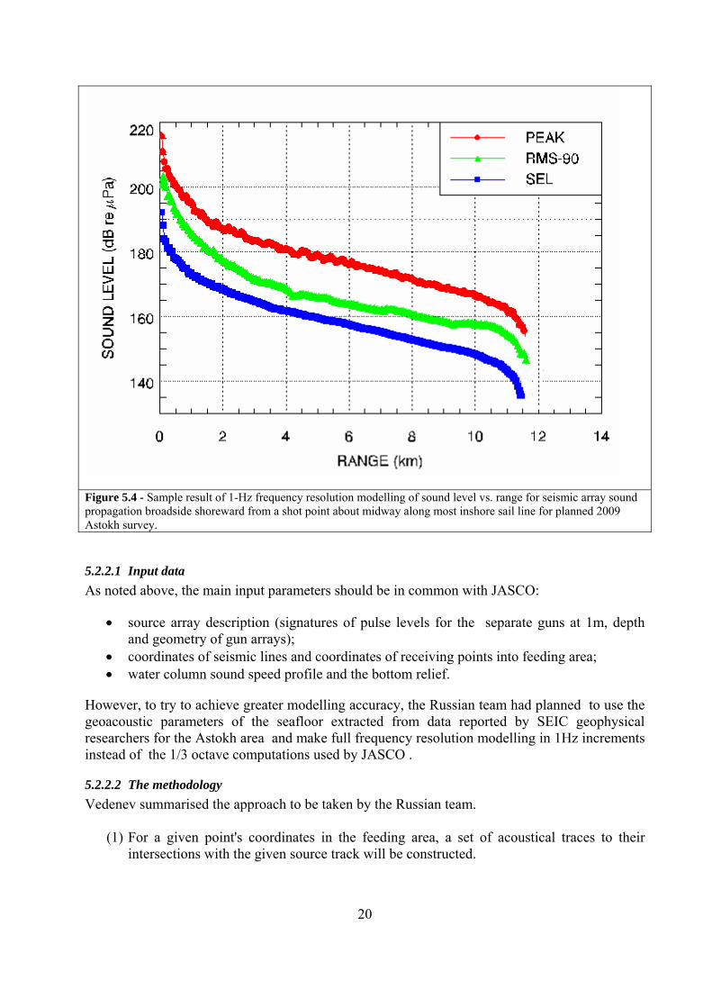
Figure 5.4 - Sample result of 1-Hz frequency resolution modelling of sound level vs. range for seismic array sound propagation broadside shoreward from a shot point about midway along most inshore sail line for planned 2009 Astokh survey.

5.2.2.1 Input data As noted above, the main input parameters should be in common with JASCO:

• source array description (signatures of pulse levels for the separate guns at 1m, depth and geometry of gun arrays);

• coordinates of seismic lines and coordinates of receiving points into feeding area; • water column sound speed profile and the bottom relief.

However, to try to achieve greater modelling accuracy, the Russian team had planned to use the geoacoustic parameters of the seafloor extracted from data reported by SEIC geophysical researchers for the Astokh area and make full frequency resolution modelling in 1Hz increments instead of the 1/3 octave computations used by JASCO .

5.2.2.2 The methodology Vedenev summarised the approach to be taken by the Russian team.

(1) For a given point's coordinates in the feeding area, a set of acoustical traces to their intersections with the given source track will be constructed.

20

21

(2) Along each trace, the acoustical environmental data needed for computation of the broadband transfer function will then be compiled: the bottom relief; the bottom sediments structure (extracted from SEIC’s geological study); and the water sound speed profile.

(3) Then the field of transfer functions from the feeding point to the positions of the

individual air guns in the seismic source array situated at the intersection of the acoustical trace with the source track will be computed, taking into account the angular position of the array. The transfer functions will be calculated using Avilov’s Pseudodifferential Parabolic Equation algorithm (see www.hlsresearch.com/oalib). The spectral contributions of all guns will be summed with phase yielding the total band sound energy from a single shot. These SELs from a single shot are then interpolated along the source track and integrated to assess the total track SEL affecting the given feeding point.

The above approach thus considers each gun as an independent source whose pressure signature is numerically propagated to a receiver location, where it is coherently summed to the signals of the other guns. This represents an alternative approach to that used by JASCO (generation of an equivalent ‘directional point source’ based on full numerical analysis of the interaction of the various airguns operating at close distance from each other) as described above. During the Workshop, Racca expressed some concerns about this alternative method, primarily as it cannot account for non-linear interaction effects in the near-field of the guns within the array. He requested additional clarification on the approach and offered to supply the Russian team with the pre-computed directional, frequency resolved source levels for the airgun array. After subsequent telephone/e-mail communications, Racca and Avilov agreed that the JASCO methodology also includes some uncertainty because the nonlinear directional characteristics are computed for a uniform unbounded medium and that this is appropriate only for the deep sea environment. In the shallow seas, those results may be compromised by: (1) the strong depth dependence of water and bottom parameters and (2) by the additional strong nonlinearity of the state equation of bottom grounds. As a result of discussion the Workshop agreed to estimate possible errors by comparing JASCO’s pre-computed directional, frequency resolved source levels for the airgun array with the linear results in the vicinity of the seismic array.

5.2.3 Conclusions and recommendations The Workshop agreed that there was merit in continuing work using both the JASCO and Russian Team approaches. It recognised the timing difficulties for the Russian Team in particular but hoped that it would be possible for at least some results to be available by WGWAP-4. For the purposes of this report, the Workshop agreed to proceed on the basis of the available JASCO modelling results.

5.3 Validation of modelling results As noted above, the predictions from the acoustic modelling play a vital role in the examination of the potential effect of seismic surveys on western gray whales off Sakhalin (e.g. see Item 7.4). It is therefore extremely important that the properties of the model(s) developed are understood and in particular that they are appropriate for the conditions off Sakhalin. Considerable discussion of this issue and the sensitivity of the modelling exercises to the chosen input parameters took place at the first meeting of the Task Force and the interested reader is directed

22

to WGWAP-3/INF.9 (and the associated appendices). At the present Workshop, greater emphasis was placed on the validation of modelling results against available measurements from previous surveys performed in the same area.

5.3.1 Comparison with 2001 data JASCO presented a comparison of the results of their propagation model with acoustic data from the 2001 ENL1 seismic survey in the Odoptu block, which recently appeared in the open literature (Rutenko et al., 2007). This is not equivalent to a direct comparison with an identical earlier survey, as the array design used by ENL had approximately half the volume of the proposed SEIC array and the area of that survey is several kilometres to the north of the planned Astokh staging. On the other hand, in the comparison JASCO used the same source modelling and sound propagation software used for the assessment of the upcoming SEIC survey, and the propagation conditions are similar in the two areas. It can therefore be argued that good overall agreement of the results in the ENL case would provide confidence in the suitability of the JASCO software and modelling approach in this setting.

The majority of the field data presented in the published study were obtained from six on-bottom acoustic monitors deployed at widely spaced locations along the 20m bathymetry line (see Figure 5.5). Each of these stations provided a time history of the received sound pulse level as the survey vessel shot a line roughly parallel to shore. Prior to the present workshop, JASCO modelled (in one-third octave bands) a scenario with the same airgun array configuration and propagation geometry, generating a series of plots (one for each station) showing the modelled per-shot levels in dB re µPa2 SEL overlaid on the processed measurement data from the study in dB re µPa RMS. A representative plot from this set is shown in Figure 5.6; the complete results are included as Annex D.

For received pulses lasting less than one second (a realistic assumption for the propagation conditions in this study), per-shot SEL levels should always be less in numerical value than the corresponding RMS metric. The model estimates, if accurately reflecting the field conditions, could thus be expected to be as much as a few dB lower than the reported measurements. The JASCO model results were in fact found to be in good numerical agreement with the ENL data, tracking the envelope of the experimentally recorded levels with consistency over the recording range except in cases where the measured levels dropped below the noise pedestal of the monitoring systems. In terms of actual acoustic levels, this indicates a tendency for the model to overestimate the measurements by a few dB. The prevailing overestimation can perhaps be ascribed to the choice of sound velocity profile for the model runs, which was based on early season conditions whereas the measurements in question took place on 8 September. The reported data from the ENL survey, however, also contain fairly intense level variations (~10 dB) occurring over the space of just a few shots (i.e. over a time scale of less than a minute and merely some tens of metres of source displacement) that are not reflected in the JASCO model results.

1 Exxon Neftegas Limited, a subsidiary of Exxon Mobil Corporation

Figure 5.5 - Map of the geometry of seismic shot line and receiver stations for the acoustic measurements performed on 8 September 2001 (from Rutenko et al. 2007, used with permission).

Figure 5.6 - Comparison of measured (RMS) and modelled (SEL) sound levels as a function of range for the 2001 ENL survey monitoring at site T.8 (original plot from Rutenko et al. 2007, used with permission).

In commenting on these results, Racca noted that the RMS metric – unlike the SEL – is susceptible to such swings since its calculation (whether based on measurement or estimation) can be affected in sudden ways by changes in the pulse length. Such changes may be physically

23

24

real, particularly in a shallow bathymetry environment where certain propagation modes can suddenly drop out as the water depth no longer sustains them. However, this argument does not seem to fully explain the sustained nature and magnitude of some of the transitions in the reported RMS levels, and it could be speculated that there may be some local propagation effects that the JASCO model did not predict with the current parameters and bathymetry database. More likely however, given the reported low signal to noise ratio of the measurements undertaken during the ENL monitoring, variability in the reported RMS levels may be an artefact of the uncertainty in identifying the start and end points of a pulse.

The Workshop also noted that on some occasions, the JASCO sound propagation model estimated lower received levels than were in fact measured (even accounting for the difference in metrics), indicating an overestimation of the local transmission loss. In a prognostic impact assessment situation, any such bias would result in the expectation of lower received levels in the feeding grounds than in fact obtain, which could lead to insufficiently stringent mitigation planning. This observation, although limited to a few instances, provided additional support for the need to test the model predictions at the beginning of the SEIC seismic survey in 2009, so that mitigation measures can be adjusted, if necessary.

During the Workshop, it was requested that JASCO perform and present an additional verification against the 2001 ENL survey study data, namely an examination of the agreement between the JASCO model output and the field measurements with respect to:

(1) the range at which the RMS level was observed to drop to 163 dB re µPa in a pre-survey calibration experiment; and

(2) the directional variation in array output (broadside vs. endfire aspect) observed during the same trials.

This request referred to a set of measurements that was conducted on 12 August 2001, after the original airgun array design had been revised to reduce its overall output (Rutenko et al., 2007).

Figure 5.7 shows a map of the location of the single receiver point used in those measurements and the track that was sailed by the survey vessel; Figure 5.8 is a plot of the received level as a function of range, directly reproduced from the referenced study.

Figure 5.7 - Geometry of seismic vessel track and receiver station for the calibration experiment performed on 12 August 2001 (from Rutenko et al., 2007, used with permission).

Figure 5.8 - Measured RMS sound levels as a function of range for the 12 August 2001 seismic airgun array calibration experiment (from Rutenko et al., 2007, used with permission).

Figure 5.8 shows that at the closest point of approach (CPA), the distance between source and receiver was 3.8km and the received level, allowing for some jitter in the individual measurements, was ~164 dB re µPa RMS. For validation modelling, the coordinates of the T.4 receiver and the sail line were obtained from the geo-referenced map; the resultant range to the CPA was 3.75km, consistent with the data. The output from the 1,640 in3 array used in the ENL survey was modelled with AASM (Airgun Array Source Model) providing equivalent directional levels; propagation modelling at 1 Hz frequency resolution was then carried out along a traverse between the CPA and the T.4 location, estimating the RMS levels at a constant depth of 20m corresponding to the bottom depth at the receiver. This was done both with the array tow axis oriented along the direction of sailing (as per actual experiment) and with the axis rotated by 90°, thus presenting the broadside and the endfire aspects of the array to the receiver. Table 5.1 shows the results of the modelling in 50m range steps for the final 250m of propagation to the receiver. The estimated final level for the array in its normal orientation (broadside to the receiver) is 165 dB re µPa RMS, within 1 dB of the measured value. Rotating the array to present its endfire aspect to the receiver causes a drop of 4 dB in the modelled RMS received level. The referenced article does not specifically state the amount of change in level that was observed at the receiver with the array rotation; this change would be influenced not only by the close-range directionality pattern of the source but also by the different spectral properties of the pulses from the two orientations. A change of 4 dB in the received RMS broadband level, however, is consistent given the reported source level difference of 6 dB between the two aspects for sub-horizontal propagation in the limited frequency band of 100-250Hz (Rutenko et al., 2007).

25

26

Model estimated received levels (dB re µPa RMS) Range (km) Broadside array aspect Endfire array aspect

3.50 166.3 162.0 3.55 166.1 162.0 3.60 165.8 162.0 3.65 165.5 161.8 3.70 165.2 161.4 3.75 164.9 161.0

Table 5.1 - Modelled received levels at 20m depth along a perpendicular radial from the source track to the T.4 receiver (located at the highlighted final range) for the 12 August 2001 calibration experiment, presenting either the broadside or endfire aspect to the receiver.

5.3.2 Comparison with 1997 data JASCO presented information on a comparison with the single available published measurement (Würsig et al., 1999) from the 1997 Astokh survey (when SEIC was operated by Marathon). This data point indicates received levels near shore at a location 30km from the seismic source that appear to be inconsistent with the JASCO modelling results.

Noting the importance of validation of the modelling results to its conclusions, the Workshop recommends that additional data points from the Würsig and Weller (1997) paper be tested against the JASCO model. Weller kindly agreed to send additional data, some of which has been received and awaits further study by JASCO as well as the Russian group. The Workshop referred specification of the workplan for this and other acoustic work to a small group comprising Nowacek, Vedenev and Racca. This is discussed further in the report of WGWAP4.

5.4 Results

5.4.1 SEIC Team Two sets of full-area acoustic footprint modelling results were presented, one for the cumulative SEL metric and one for the envelope of single-shot SEL. Both were obtained by modelling the directional spectral source levels of the planned 2620 in3 airgun array, propagating them along radials in one-third octave bands and either cumulating or merging the results as described in an earlier section. Figure 5.9 shows the cumulative SEL footprint for the assumed maximum exposure scenario for the feeding area over a 24 hour period: a racetrack pattern starting with the most inshore survey line, followed by a return line 7km farther offshore (at the optimal turning diameter), followed by the secondmost inshore line at 300m spacing from the first. The footprint is only developed on the shoreward side of the outermost line, which is sufficient for the purpose of exposure assessment over the feeding area.

After considerable discussion of the merits and difficulties of adopting any mitigation measures based on cumulative exposure criteria, the Workshop concluded that reverting to widely adopted and better understood criteria based on single-pulse levels would be the more precautionary decision in the face of insufficient scientific data to support a different approach (for details of the discussion, see Item 6). Given this, attention shifted to the envelope footprint from all shots along the most inshore survey line (Figure 5.10) which constitutes the locus of maximum single-pulse exposure for animals within the feeding area as the line is sailed. The values are maximized over depth so that contour boundaries represent the maximum planar extent of exposure to a given intensity level regardless of the depth at which whales may be at the moment of exposure.

Figure 5.9 - Modelled footprint of cumulative SEL from the two most inshore survey lines and a reciprocal line 7km

farther offshore. Only propagation on the shoreward side of the outer line is considered. Levels are in dB re µPa2-sec.

Figure 5.10 - Modelled envelope footprint of single-pulse SEL from all the individual shots along the most inshore

survey line. Levels are in dB re µPa2-sec.

27

The results from one-third octave band area modelling are in units of SEL, whereas behavioural impact thresholds are commonly expressed in terms of the RMS metric (see Item 6). To allow an impact estimation boundary to be defined in terms of modelled SEL contours, site-specific conversion offsets between the two metrics were estimated as described above. Of greatest importance for population impact assessment within the feeding area is the shoreward front of the 163 dB RMS level; to define it with accuracy, 1Hz resolution modelling was performed for a set of nine broadside pulse propagation radials extending shoreward from shot points along the most inshore survey line. The analysis showed that for all these radials the RMS and SEL metrics exhibited an essentially constant difference of 7 dB at the propagation range to 163 dB re µPa RMS. This finding allowed the use of the third-octave modelled contour for 156 dB re µPa2 SEL as a surrogate (at least in the shoreward propagation direction) for its 163 dB re µPa RMS counterpart. A few additional 1 Hz resolution model runs were performed to determine whether the difference might be higher for more slanted propagation radials at the extremities of the footprint, which would have required conversion to a lower SEL contour (larger range) in those sectors; the results showed instead that the 156 dB SEL contour proxy constituted a precautionary upper limit in other directions. This approach allowed the definition of a formal limit line for behavioural impact that was used in the density based assessment described under Item 7.4.1.

28

5.5 Real-time calibration issues (comparison of modelling results with real-time measurements)

As discussed under Item 5.3, the SEIC modelling efforts have provided estimates of the sound levels that are expected to impinge on the feeding area during the 2009 survey. As with any model, however, the Workshop acknowledged that it is essential to calibrate the model results in situ using the actual airgun array source. If the model results are further validated, no modification of the monitoring and mitigation protocols discussed under Item 7 will be required and vice versa. To this end, the Workshop discussed several aspects of real-time calibration, including equipment and procedures.

SEIC informed the Workshop that the instruments to be used are essentially those that have been used for past acoustic monitoring, but that the transmission to shore over the radio modems will probably be digital rather than analogue. Additionally, SEIC is considering using a repeater system given the distances involved, particularly between the southernmost buoys and the light house where the monitoring personnel and equipment will be based. The goal is to have full waveform transmission so that the characteristics of the signals can also be monitored. SEIC consider this to be important so that ‘non-SEIC’ noise can be monitored separately. Vedenev commented that there was value in transmitting processed rather than raw data, but SEIC considers it feasible and ultimately preferable to transmit full waveform information.

The buoys will be calibrated initially by the Pacific Oceanological Institute (POI) at their facility and then again in situ after deployment, using a sound source of precisely known characteristics. Acoustic monitoring stations will also be deployed within the feeding area, near the 10m isobaths; these will be archival recorders (see Item 7.5.1).The digital buoys and the transmission system will operate with 16 bit precision, providing a potential dynamic range of 96 dB. The Workshop was assured that all of the data collected by all of the buoys, including the ‘joint program study’ sensors during the entire survey period will be readily available to SEIC, its contractors and the WGWAP. The Workshop agreed that access to these data are critical so that any potential effects on whales present can be analyzed, and the full dose of the survey at the edge of and within the feeding ground can be calculated.

In discussion, SEIC noted that in addition to the fixed receivers it was possible to have acoustic monitoring equipment on the zodiacs or small boats deployed to monitor at/near the acoustic monitoring line and/or near whales in the ‘buffer zone’ between the monitoring line and the 163 dBRMS isopleth. They commented that such equipment would not be the principal decision-making tool – it would only be used as a learning tool. The Workshop agreed that if the buoys are tested and calibrated, additional acoustic equipment on the zodiac during the real-time calibration exercise was not necessary. However, it was suggested that this additional recording capability should be retained during the monitoring of the survey

With respect to the issue of contaminating noise recorded by the buoys, Racca described the pyramid structure that is used to keep the hydrophones off the bottom. SEIC welcomed any suggestions for ways to minimize the flow noise received by the stations. This is particularly important given the low frequency nature of much of the energy from seismic surveys.

In conclusion, the Workshop recommended the use of digital data transmission radio acoustic buoys in the 2009 seismic survey for real-time acoustic monitoring. It noted that modern radio acoustic buoys are equipped with an industrial PC and HD- or SSD-based recording system to store all acoustic data and radio or satellite modems to transfer measurement data. In the direct

line of sight, radio modems can transmit either seismic pulse parameters (RMS, SEL levels, averaged spectra) or initial measurement data (raw data). One benefit of transferring pre-averaged parameters is a dramatically reduced data flow. For example, at the 4kHz digitization frequency, the ‘raw’ data flow will be 720 Kb/min. However, seismic pulse and averaged spectrum (up to 500 Hz) data transfer is less than 1 Kb. It significantly improves data transfer reliability under atmospheric disturbances because it supports repeated data package transmissions, effectively preventing loss of data. Averaged spectrum analysis produces confident hydrophone flow noise classifications (manifested at 20-30 Hz) and dismisses elevated noise level periods not associated with seismic survey pulse. This methodology was tested during acoustic monitoring of the Piltun area during maritime facility construction in 2005-2006. Figure 5.11 illustrates regular increases in the low frequency components of the spectrum during stronger tide currents. These data segments were removed during industrial noise monitoring.

Figure 5.11 - Example of regular increases in low frequency components during strong tidal currents

29

30

6 FURTHER CONSIDERATION OF THE DOSE-BASED APPROACH

6.1 Literature review The literature relevant to the dose-based approach discussion is adequately treated in (Southall et al., 2007), and the reader is referred to that paper, Seismic TF 2/Doc.5 and WGWAP-3/INF.9 for a full discussion of the most recent efforts to define noise exposure criteria for marine mammals and the use of a dose-based approach. Given the extensive literature review undertaken at the first workshop (WGWAP-3/INF.9), the present Workshop agreed that there was no need for a similar review to occur here. The focus of the Southall et al. (2007) paper was to make initial recommendations regarding noise exposure, although the authors do develop a strong case for the use of a dose-based approach to the setting of criteria, based largely on data from humans and laboratory experiments with other mammals. In summary, there is uncontroversial evidence that people and the animal species tested demonstrate responses which indicate that it is essential to measure noise dose, rather than simply instantaneous exposure. In the cases examined by Southall et al., accumulated doses were shown to be able both to affect hearing (e.g. causing injury to the auditory system after prolonged exposure), and to induce other ‘non-auditory’ effects (e.g. release of stress hormones, reduced sleep and other physiological consequences).

There was some discussion of the issue of hearing loss caused by cumulative noise. It was noted that hearing loss in humans can accumulate over several years. In terms of assessing potential effect of noise on cetaceans, and developing mitigation measures, it is important to try to determine a sensible ‘accumulation period’ and in particular to agree on what exposure is acceptable in a single survey.

In the absence of appropriate data for cetaceans, the Workshop agreed that adopting a 24 hour period was a practical approach. This was chosen primarily due to its ubiquitous use in workplace regulations, its use in other similar marine mammal applications (see Southall et al., 2007) and because it is difficult to define another period that is feasible to use given the uncertainty and variability associated with the operation of the survey, e.g., unforeseen stand-down periods due to weather.

The Workshop also considered whether it was appropriate to equate multiple pulse situations with continuous noise. It was noted that the mammalian auditory system responds differently to stimuli that present continuous vs. intermittent pulsed energy (although the behavioural consequences of such a difference is not well understood for marine mammals). The Workshop agreed that at present at least, it was not appropriate to consider multiple pulses as continuous noise.

In conclusion, the Workshop reaffirmed that in principle, a dose-based approach is appropriate (and see WGWAP-3/INF.9). Unfortunately, it must be recognized that in the recent comprehensive review by Southall and colleagues, the authors were unable to recommend a dose-based criterion for behavioural disturbance for ‘low frequency’ cetaceans, such as gray whales, exposed to multiple pulse noise.

The Workshop adopted the proposal of Southall et al. (2007) with respect to dose-based criteria for permanent auditory injury (PTS) for ‘low frequency’ cetaceans: 198 dB re 1 µPa2-s (SEL).

31

6.2 Discussion and implications/recommendations for forthcoming survey Given the agreement on the Southall et al. criteria above, the Workshop examined a plot provided by Racca (Figure 5.9) showing the estimated cumulative exposure obtained by considering the two shot lines nearest the feeding area and one line sufficiently offshore to allow for a ‘race track’ turn i.e., the maximum dose that could be expected in a 24 hr period. Workshop agreed that the 198 dB re 1 µPa2-s cumulative SEL threshold for PTS onset is not encountered until ca. 1 km inside the boundary to 180 dBRMS re 1 µPa received level as estimated by modelling.

Given the agreement in principle over using a dose-based approach but the inability of Southall et al. (2007) to provide a recommendation for behavioural disturbance, it was agreed that it was important to examine whether it was possible to develop a scientifically justifiable dose-based criterion. A small group appointed by the Chair undertook a detailed review of the relevant Malme et al. papers (Malme et al., 1986; Malme et al., 1988) - the origin of the primary field data on gray whale responses). They considered two possible methods for developing a dose-based criterion.

The first potential method resulted from additional information kindly provided to the Workshop by Dr. Malme via email. He reported that the first observed behavioural disturbance occurred at a RL of 149 dB (corresponding in their experiments to a range of 4 km) and all whales had responded by the time the RL reached 176 dB (range 0.7 km). Other available information included: the published information on a 10% response at 163 dB and a 50% response at 173 dB; the speed of the vessel used; the number of pulses emitted per minute; and information on the nature of the pulses. It had been hoped that this information would allow estimation of the dose received by each ‘group’ of responding whales (i.e., the number of pulses and therefore the energy received by those that responded at 149, 163, 173, and 176). However, further inspection revealed that the vessel approaches that resulted in the documented responses occurred on different days i.e. the distance between a given whale and the vessel at the beginning of the approach was unknown. Given this, the Workshop agreed that dose could not be estimated by this method.

The second potential method was based on an approach used by the U.S. Navy to assess the risk to animals exposed to multiple sonar pings in an environmental impact statement (Jenkins, 2005). Of course, seismic pulses are quite different but they are also produced in a repeated fashion. The formula used was:

P = (SPP) + 5 log(n).

Where: ‘P’ is the permissible level (i.e. beyond which mitigation measures would be triggered); ‘SPP’ is the single pulse permissible level (i.e. the level for a single pulse that is considered to be acceptable); and ‘n’ is the number of received pulses. The benefit of such an approach is that in addition to tracking an exposure dose, it should be easy to implement in the field. However, the Workshop agreed that the formula’s inability to account for the changing amount of energy contained in the pulses as the seismic vessel approached and passed an animal or monitoring station rendered it inappropriate.

The Workshop thus had no basis for creating a new dose-based threshold for behavioural disturbance and it therefore agreed to:

32

(1) use the widely accepted standard of 163dBRMS as a behavioural disturbance threshold (from the limited data available, this corresponds to a probability of 0.1 that a whale will cease feeding upon receiving such a level – it was also noted that all of the whales displaced from feeding in the Malme et al. studies returned to feeding after the pass of the seismic vessel; and

(2) given the need to develop a dose-based approach, measures of dose should be included in the monitoring effort of the 2009 survey as well as the subsequent data analysis.

With respect to (1), although it is thought that current authorizations by the U.S. National Marine Fisheries Service call for a behavioural disturbance threshold for seismic surveys conducted near gray whales of 160dBRMS, the Workshop agreed that the 163dBRMS level was appropriate. There is no scientific rationale for 160dBRMS, other than perhaps it is below the 0.1 probability of disturbance. As noted above, the first response observed by Malme and colleagues was at 149 dBRMS and thus the 160dBRMS level will not necessarily prevent all disturbance. In addition, it was recognised that significantly more mitigation measures will be in place (see Item 7) for the proposed 2009 surveys than are commonly employed for seismic surveys, providing additional assurance that as few whales as possible will be exposed even to the 163dBRMS level. For example, during ‘normal’ seismic surveys there is little or no effort made to watch for whales in the area ensonified near 160dBRMS whereas during the proposed SEIC survey, the section of the feeding area ensonified at 163dBRMS or above will be monitored visually and acoustically. It is important to use experience to inform our threshold/criteria. The 2001 ENL survey used a threshold of 163dBRMS at the 20m contour, but, as noted under Item 4, there are now many more years of whale distribution to inform decisions on the area to be protected from levels above the 163dBRMS threshold. This is considered further under Item 7.4.

In relation to (2), the Workshop also agreed to examine the expected dose during the survey to the extent that it would express levels using the SEL (sound exposure level) as well as RMS metrics. In doing this, it is stressed that RMS is location-related; SEL is not being used as a synonym of dose (note that JASCO has calculated SEL on a per pulse basis unless otherwise specified).

Given the extensive modelling of the source and propagation, an interest was expressed in pursuing the use of the dose-based approach. It was recognised that given time constraints, any such efforts would be outside the Task Force process; however, the results might be of interest within the WGWAP process.

7 MITIGATION AND MONITORING The basis for the discussions under this item were the discussions and recommendations made at the first meeting of the Seismic Task Force (WGWAP-3/INF.9).

7.1 Summary of existing mitigation measures The Workshop was pleased to receive a summary of international requirements for mitigation measures (Seismic TF 2/Doc. 10) and thanked Angelatos for compiling this.

7.2 Objectives In an ideal situation i.e. one with adequate information on the short-, medium- and long-term effects of seismic surveys on western gray whales, specific conservation targets would be set (e.g. maximum number of whales that may be exposed to certain doses of sound). The task

33

would then be to devise mitigation measures to ensure that these objectives were met (with sufficiently high probability), and to specify monitoring arrangements that would help to verify the extent to which the targets were met.

However, as discussed under Item 6, there is considerable uncertainty surrounding the appropriate sound levels, even for short-term behavioural responses and even less information is available on the long-term effects at the population level, if any.

Under such circumstances, the Workshop agreed to take a pragmatic approach i.e.

(1) specify mitigation measures that it agreed were reasonable and practical;

(2) provide an indication of how these measures may limit or reduce the exposure of the whales to different sound levels.

The Workshop concurred with the approach identified in WGWAP-3/INF.9 i.e. use current best practice as the starting point for its recommendations on mitigation methods, improving on this where clear weaknesses have been identified.

The general objectives of the mitigation strategy are twofold:

(a) to reduce the risk of exposure of whales anywhere in the survey area to dangerously high noise levels that might cause auditory injury;

(b) to limit the exposure of whales to noise on the feeding ground, with the aim of limiting adverse behavioural consequences of noise exposure that might reduce feeding success, especially for mothers with calves.

With respect to objective (a), the Workshop agreed that, in line with current practice, an exclusion zone based on the 180dBRMS re 1 μPa isopleth be implemented throughout the survey (such that shutdown occurs when a whale is detected in this zone), and that additional measures be implemented for survey conducted at night or in fog when whales cannot be detected directly.

The size of the exclusion zone will be determined by direct measurement of the range at which the airgun array sound level drops below the 180 dBRMS re 1 µPa threshold at the broadside maximum, plus a precautionary margin of 20% to be applied if the measured range is less than 1.7 km; this zone will have a minimum radius of 1 km. Until this range is determined, a fixed exclusion zone of 2.0km will be observed.

With respect to objective (b), the Task Force proposed that additional mitigation measures be taken when real-time monitoring indicates that received sound levels may exceed 163 dBRMS re 1 μPa per pulse (see discussion under Item 6) in any part of the feeding ground (as delineated by the boundaries developed under Item 7.4.1.1 for the periods June-July or August-September, as appropriate).

7.3 Background information

7.3.1 Estimation of detection function of MMOs This issue is examined in Annex E and was considered in the context of Item 7.4.2.

34

7.3.2 Technical issues surrounding real-time acoustic monitoring The Workshop referred to its discussions and recommendations under Item 5.5.

7.4 Examination of risk

7.4.1 Use of whale density data to delineate the feeding area and assess potential impacts of the 2009 SEIC seismic survey

7.4.1.1 Proposed Piltun feeding area perimeter monitoring line

The Workshop recommended that sound levels at the edge of the Piltun feeding area be monitored in real-time using acoustic receivers stationed along the feeding area boundary (see Item 7.5.1). The Workshop agreed that the perimeter monitoring line for the Piltun feeding area should be delineated using the method described below. At the time of the Workshop, it was only possible to undertake this for the datasets for which associated effort was already available – updated analyses using the additional data referred to under Item 4.1 will be undertaken by Muir in co-operation with the Advisory Group and updated perimeter lines delineated.

(1) A 1.0 km × 1.0 km grid of average estimated whale densities in the Piltun feeding area was produced for each year of 2005 to 2007, based on the systematic aerial, vessel and shore-based survey data using the methods described above. In addition, a grid of the maximum estimated density in each grid cell that was estimated by any survey during 2005 to 2007 was calculated, as a precautionary sensitivity test. The four density grids were determined for two time intervals:

(c) 1 June to 31 July – the period during which the seismic survey is planned to take place and when gray whales are migrating into the Piltun area and the number of whales is low;

(d) 1 August to 30 September – the period when whale abundance in the Piltun area is stable and at its highest numbers; assessed to allow for the possibility that poor weather conditions may delay the start of the seismic survey.

(2) A 95% kernel density contour was determined for each density grid produced in step (1), using the ArcView 3.2 Animal Movement extension with a 1 km cell size and user selected smoothing factor (H) of 1000m (Hooge and Eichenlaub, 2000). The smoothing factor of 1000m was a conservative measure that was selected to allow for error in estimating whale sighting distances from an observer when using reticle binoculars during the systematic surveys. Kernel density methods are statistical techniques to estimate a probabilistic density surface of an animal’s or population’s distribution (Seaman et al., 1998). The probabilities indicate the relative amount of time spent at a location (Seaman et al., 1996).

(3) The offshore segment of each kernel density contour that extended 10km north and 10km south of the shot area centre was then extracted to delineate the Piltun feeding area perimeter monitoring line.

The 95% kernel density contours were visually inspected to assess the sensitivity of the offshore edge of whale distribution to effects of year, and to use of average densities compared to maximum densities. Yearly and maximum density kernels for the June-July time interval were quite similar in the vicinity of the planned 2009 seismic survey. Yearly and maximum density kernels for the August-September interval were more variable, particularly in 2006, with gray

35

whales distributed approximately 1km farther offshore in the vicinity of the seismic survey area compared to the other years.

As a precautionary approach, the Workshop recommends that two (one for June-July and one for August-September) perimeter monitoring lines be designated, using the kernel density contours based on maximum gray whale densities for that time interval. The perimeter monitoring line used during the seismic survey will correspond to the time period during which the seismic survey begins. As examples only, the maximum whale densities by grid cell based on the presently available 2005 to 2007 June-July data set or the data from August-September (Fig. 7.1), are overlain on a map of the area, along with the 156 dB SEL2 sound contour for the 2008 Astokh seismic survey that was estimated to be equivalent to the 163 dBRMS sound contour along the shoreward front and a conservative proxy to it at the north and south ends. The Workshop recommends that the two boundaries that will be produced by the updated analyses (see Item 4.1) be adopted in the context of the mitigation measures described below.

7.4.1.2 Use of the density data to assess potential impacts from the 2009 survey

The average and ‘maximum’ whale densities estimated at a 1 km2 resolution from systematic aerial, vessel and shore-based survey data collected from 2005 to 2007 (see above) were used to assess the potential impacts on gray whales from the planned 2009 SEIC seismic survey during June-July, and again for August-September.

The modelled 156dBB

SEL sound contour was used as the area boundary for these calculations as a proxy for the 163dBRMS sound level. This contour was determined through fine frequency resolution modelling to be equivalent to 163dBRMS threshold along the shoreward front, and a precautionary estimate at the north and south ends. Consequently the June-July non-zero average density cell located approximately 6 km north of the perimeter monitoring line was safely excluded from the estimate of potentially impacted whales during June-July, since it lies fully outside the 156 dB SEL boundary. Conversely, the August-September non-zero density cell located approximately 2.5 km northeast of the northern end of the perimeter monitoring line was retained on a precautionary basis in the calculations of potentially impacted whales during August-September, since it lies just inside the 156 dB SEL boundary.

The analysis was repeated using maximum estimated whale densities for each time interval, to determine a precautionary estimate of the maximum daily number of whales potentially impacted. The maximum density in each grid cell was determined by taking the maximum density estimated for that grid cell by any survey during the time interval in question. Thus the maximum densities do not provide a snapshot of gray whale abundance during any one survey, but instead represent a composite of the maximum values that have been calculated for each grid cell over multiple surveys during 2005 to 2007. Consequently the estimate of potentially impacted whales using this metric provides an upper bound on potential impacts to gray whales (and one that is highly unlikely to occur).

2 Sound Exposure Level

36

Figure 7.1 - June-July (left) and August-September (right) maximum estimated whale densities based on 2005 to 2007 data (see Item 4) are shown overlaid with the 2009 seismic survey area and the predicted noise front for the portion of the 156 dB SEL acoustic contour that is either equivalent to (solid line along the shoreward front) or a precautionary estimate of (dashed line at the north end) 163 dB RMS. The maximum density estimated by any survey is shown for each grid cell. The perimeter monitoring line for acoustic receivers was delineated by first deriving a 95% kernel density contour for the 2005 to 2007 maximum estimated densities for the appropriate time interval, and then extracting the offshore segment of the contour that extended 10 km north and 10 km south of the shot area centre.

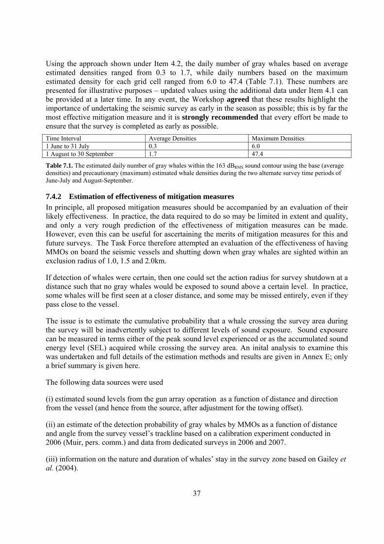
37

Using the approach shown under Item 4.2, the daily number of gray whales based on average estimated densities ranged from 0.3 to 1.7, while daily numbers based on the maximum estimated density for each grid cell ranged from 6.0 to 47.4 (Table 7.1). These numbers are presented for illustrative purposes – updated values using the additional data under Item 4.1 can be provided at a later time. In any event, the Workshop agreed that these results highlight the importance of undertaking the seismic survey as early in the season as possible; this is by far the most effective mitigation measure and it is strongly recommended that every effort be made to ensure that the survey is completed as early as possible. Time Interval Average Densities Maximum Densities 1 June to 31 July 0.3 6.0 1 August to 30 September 1.7 47.4

Table 7.1. The estimated daily number of gray whales within the 163 dBBRMS sound contour using the base (average densities) and precautionary (maximum) estimated whale densities during the two alternate survey time periods of June-July and August-September.

7.4.2 Estimation of effectiveness of mitigation measures In principle, all proposed mitigation measures should be accompanied by an evaluation of their likely effectiveness. In practice, the data required to do so may be limited in extent and quality, and only a very rough prediction of the effectiveness of mitigation measures can be made. However, even this can be useful for ascertaining the merits of mitigation measures for this and future surveys. The Task Force therefore attempted an evaluation of the effectiveness of having MMOs on board the seismic vessels and shutting down when gray whales are sighted within an exclusion radius of 1.0, 1.5 and 2.0km.

If detection of whales were certain, then one could set the action radius for survey shutdown at a distance such that no gray whales would be exposed to sound above a certain level. In practice, some whales will be first seen at a closer distance, and some may be missed entirely, even if they pass close to the vessel.

The issue is to estimate the cumulative probability that a whale crossing the survey area during the survey will be inadvertently subject to different levels of sound exposure. Sound exposure can be measured in terms either of the peak sound level experienced or as the accumulated sound energy level (SEL) acquired while crossing the survey area. An inital analysis to examine this was undertaken and full details of the estimation methods and results are given in Annex E; only a brief summary is given here.

The following data sources were used

(i) estimated sound levels from the gun array operation as a function of distance and direction from the vessel (and hence from the source, after adjustment for the towing offset).

(ii) an estimate of the detection probability of gray whales by MMOs as a function of distance and angle from the survey vessel’s trackline based on a calibration experiment conducted in 2006 (Muir, pers. comm.) and data from dedicated surveys in 2006 and 2007.

(iii) information on the nature and duration of whales’ stay in the survey zone based on Gailey et al. (2004).

38

Using this information, and assumptions about the shut down process, seismic vessel speeds and survey strategy (whole area covered, lines 300m apart), a simulation study was conducted as described in Annex E.

As noted in Annex E and during discussions of it, a lack of sufficient data with respect to estimating MMO effectiveness and detection functions, and a number of other assumptions that had to be made, precluded detailed quantitative consideration of the results. However, the general pattern is clear: some whales will not be detected until they are well inside the selected shutdown radius, especially for lager radii. In the simulations, some whales received doses believed sufficient to cause TTS or even PTS, even when the sound level at the nominal shutdown radius is well below this. However, the effect of the shutdown radius is to substantially reduce the expected number of such incidents.

The Workshop agreed with the general conclusion of the Annex that whilst having an exclusion radius monitored by MMOs was not a perfect mitigation measure, it was certainly helpful. It does not obviate the desirability of finding alternative survey technologies that do not involve injecting such large volumes of sound into the water column.

The Workshop agreed that the approach outlined in Annex E was valuable and that it was worth investigating what (and how) additional data could be obtained to improve the analysis in the future. Particular emphasis was placed on the need to obtain better information on the MMO detection function and their ability to estimate distances in the field. It was noted that the 2008 field season could be an appropriate time to carry out experiments in this regard (either an updated calibration exercise or an alternative approach e.g. using double-observer methods). There was insufficient time to develop this further within the Task Force. Additional suggestions for data that would improve the analysis included better transmission loss information.

7.5 Monitoring (number, distribution, behaviour) One of the major difficulties faced by the Workshop in assessing the risk to western gray whales from seismic surveys (and indeed any anthropogenic noise) was the shortage of applicable data on effects of sound on baleen whales. Given that regular (4-5 years) seismic surveys are expected for the lifetime of the field the Workshop agrees that it is essential that every effort is made to ensure that the WGWAP (or any other body) does not find itself in the same position the next time a seismic survey is proposed. It is thus of great importance that a sufficient monitoring effort is in place to maximise the collection of relevant data to allow a better analysis of the problem and thus develop better mitigation measures for the future.

The Workshop had neither the time available nor the necessary analytical expertise available to develop a detailed monitoring plan. What is described below should rather be considered general principles. It strongly recommends that a suitable group of experts be asked to work with SEIC scientists to develop a fully specified field plan and proposed analysis, well before the final plans for monitoring in 2009 are completed.

The Workshop emphasises that the monitoring measures proposed are not only related to scientific matters but are integrally related to the mitigation measures proposed or likely to be proposed for future surveys. Indeed, most of the monitoring measures provided below are essential for implementation of the mitigation measures proposed under Item 7.6.

The monitoring measures proposed by the Workshop can thus be said to fall into two categories:

39

(1) real-time monitoring required to detect when the conditions for shut down are triggered (i.e. essential for mitigation);

(2) additional monitoring (involving the collection of some data that do not need to be analysed in real time) to obtain data on the effects of the seismic survey on whales, especially western gray whales, to add to the existing knowledge base, and to contribute to the design of mitigation strategies for future seismic surveys.

7.5.1 Acoustic monitoring (perimeter and within area)

7.5.1.1 Along the perimeter of the feeding area (1) Real-time monitoring of acoustic levels using sea-bottom receivers will be undertaken

during all periods of seismic source activity.

(2) A total of at least nine receivers will be positioned at 2500 m intervals along the edge of the feeding area to ensure adequate redundancy. There will thus never be more than 5000m between active buoys (considered the range of reliable model-based interpolation of recorded sound levels).

(3) Receivers will be in place and verified to be functioning properly before activity starts and for the duration of the survey.

(4) There will be a direct radio link between the real-time monitoring acoustician and the Senior MMO on the active seismic vessel.

7.5.1.2 Within the feeding area (1) All necessary efforts will be made to obtain archival acoustic data within the feeding area

using bottom-mounted receivers.

(2) During the seismic survey, ≥3 acoustic monitoring buoys will be deployed in the feeding area on or near the 10m isobaths and near the centre of the field of view of the shore stations. Verification that these buoys are operational during the survey should be undertaken, at least at the start of the survey.

7.5.2 General visual monitoring (shore-based and vessel-based) Note that whilst the monitoring below focuses on the area within the feeding area near to the seismic operations, the Workshop agrees that it is also important to maintain the observation effort throughout the rest of the area as in previous years. This is important for analysing and interpreting the data with respect to actual or potential effects of seismic surveys on the whales, and for maintaining the longer-term monitoring data series that will be a valuable resource when future seismic operations occur.

7.5.2.1 Within the feeding area (shore-based) (1) Shore-based scan surveys will be undertaken by two teams at the five pre-existing vehicle

scan observation points south of the mouth of the Piltun lagoon (i.e., vehicle scan survey observation stations 9 to 13) to enhance the resolution of potential changes in whale density and distribution. The timing of scans will be scheduled to ensure the monitoring of whales pre-, during and post seismic line acquisition. Pre- and post surveys will be conducted 1 hour prior/post of the acquisition whilst ‘during’ scans will be conducted 1 hour from the onset of line acquisition. A third team will conduct daily surveys, weather permitting, at the eight pre-existing vehicle scan observation stations north of the mouth

40

of the Piltun lagoon (numbers 1 to 8) using the same survey protocols as in previous years.

(2) Behaviour will be monitored by two behavioural monitoring teams. The location of behavioural platforms will be directly inshore of the seismic activity in areas that are expected to have the highest exposure levels. Scans conducted by behavioural monitoring teams will augment information on whale numbers collected by the shore-based distribution surveys.

7.5.2.2 Within the feeding area (vessel-based) (1) Behaviour will also be monitored from a vessel platform. This will cover whales that may

occur near or slightly outside the defined feeding habitat that are not being monitored effectively by shore-based teams (e.g. due to low station heights, onshore fog etc). The monitoring location will be within regions of maximum predicted ensonification. The vessel type should be selected based on requirements of minimal sound output with an effective observation height (5-10 m) to increase the range of whale observations. Focal follow observations will be conducted from this platform to monitor respiration patterns and the general movement of the whales in the specified region. Extended focal follows should be conducted on whales displaying aberrant movements and/or behaviour to monitor potential long-term responses. The vessel will maintain a distance of at least 1 km from the whale being observed.

(2) Gray whale distribution will also be monitored from a vessel platform in the event of inclement weather (e.g. onshore fog) that prevents the monitoring described in section 7.5.2.1.

(3) The observation vessel will have a direct radio link to the Senior MMO on the active seismic vessel.

7.5.2.3 Within the proximity of the seismic related vessel(s) (1) Experienced MMOs will be stationed on all vessels (i.e. seismic, scout and supply

vessels) for the duration of the survey.

(2) MMOs will be limited to a maximum 2-hour continuous shift with a minimum of 1 hour between shifts.

(3) Single-point authority for operational shutdown will lie with the on-shift Senior MMO on the seismic vessel.

(4) All vessels and real-time acousticians will have direct radio access to the on-shift Senior MMO.

(5) MMO observation platforms should be located at the highest elevation available on each vessel with the maximum viewable range from the bow to 90˚ port/starboard of the vessel. Optimal locations might be on the ‘flying bridge’. Use of the bridge should be avoided due to obscured views and potential distractions.

(6) An extended visual search (20 minutes) will be conducted prior to start-up of the seismic source.

(7) There will be a minimum of two MMOs on watch on the seismic vessel at any given time during ramp-up, shooting and for the 20 minutes before start of ramp-up.

41

(8) Occurrence and behaviour of whales will be documented in accordance with existing MMPP (Marine Mammal Protection Plan) and MMO procedures.

7.6 Mitigation measures

7.6.1 Timing of surveys (1) The seismic survey will commence and be completed as early in the season as logistically

possible. Logistics include ensuring that all mitigation and monitoring procedures are in place.

(2) The duration of the seismic survey will be as short as technically and logistically feasible. Logistics includes ensuring that all mitigation and monitoring procedures are implemented fully.

(3) Lines in Zone A (see Item 7.6.2.1 below) should be acquired at the earliest possible opportunity given visibility, mitigation and monitoring requirements.

7.6.2 General design and conduct of surveys The Task Force agreed that the most stringent mitigation measures should be applied in Zone A as defined under Item 7.6.2.1. The monitoring measures defined under Item 7.5 must be in place and operational for the acquisition of lines.

7.6.2.1 Definition and updating of A and B zones (1) Initially, the survey area for which the additional mitigation measures are in effect (A

zones) will be defined by the overlap of the ‘feeding area’ and the maximum shoreward extent of the 163 dBRMS isopleth for that particular shot line.

(2) Before any lines are shot within the range currently predicted to exceed 156 dBSEL at the perimeter monitoring line, received sound levels at the line will be compared with model predictions. If received sound levels exceed model predictions, then the model shall be retuned to match the observed levels. Based on the updated model predictions, shot lines for which an overlap is predicted between the 163 dBRMS contour and the monitoring line will be reclassified as A lines, for which the additional mitigation measures specified below apply.

(3) The comparison between observed and expected sound levels at the perimeter monitoring line, and, where indicated, retuning of the acoustic model, shall be repeated at regular intervals during the survey.

(4) In the event that the 163 dBRMS threshold is exceeded at any receiver on the edge of the feeding ground while shooting a B line, operations shall be suspended immediately or shifted away from the feeding ground until a recalibration exercise has been conducted as described above, and the lines have been reclassified accordingly.

7.6.2.2 Measures within the proximity of the seismic vessel – entire survey (1) After more than 20 minutes of inactive source, ramp-up procedures will be adopted such

that the individual air guns will be activated in a progressively larger combination over a period of several minutes (6 db increments every 5 minutes over 20 minutes).

(2) The Senior MMO will initiate source shutdown if a gray whale is observed within defined exclusion radius of the source array.

42

(3) The Senior MMO will initiate a precautionary shutdown if a gray whale is observed to be on a course that will result in it entering the shut down zone.

(4) Low level single (smallest) gun operations will be conducted during line changes. Ramp-up procedures will furthermore be implemented 20 minutes prior to the sequential line acquisition. As long as the single gun operation is uninterrupted during the line change, this period will not be interpreted as ‘source inactivity’ for the purposes of clause (5) below.

(5) For operations in conditions that preclude effective visual monitoring of the defined exclusion radius of the source array (e.g. night, fog, poor visibility3)

(a) Prior to a seismic acquisition, the line of interest will have been surveyed (if necessary using a second vessel) at most 6 hours preceding the start time of acquisition of the line to ensure that no gray whales have been sighted in the vicinity of the line. If poor visibility hampers survey of the entire line, then the line will not be acquired.

(b) Operations will shut down for the night period if whales are sighted in the pre-dusk scan.

(c) After more than 20 minutes of source inactivity, operations will not be re-commenced, due to the inability to conduct an adequate visual scan.

7.6.2.3 Additional restrictions for Zone A (1) No acquisition during periods of poor visibility3 or at night

(2) No acquisition unless the feeding area perimeter line is within the effective sighting distance of a shore station or an additional vessel.

(3) No acquisition if any gray whales have been observed in Zone A over the preceding 6 hours.

(4) No acquisition if mother-calf pairs have been observed in Zone A in the preceding 12 hours.

8 CONCLUSIONS In concluding, the Chair noted that the Workshop had carried out a substantial amount of work. In particular the analyses incorporating the whale density data (Item 4) and the acoustic

3 “Poor visibility” means any conditions under which the estimated distance at which a gray whale can be reliably sighted is less than the defined exclusion radius. A prohibition on night shooting could increase the survey duration by up to 50%, which would be undesirable, both in terms of increased costs and in terms of extending the duration of the seismic survey into the period of peak whale abundance. The Workshop therefore agreed that night shooting or shooting during fog or poor light should only be conducted when the line has been surveyed (either by a separate “scout” vessel or while shooting an adjacent line) in good conditions during the preceding six hours and no gray whales have been sighted within this period. This would be the first time such a measure has been tried: the period of 6 hours, while considered practical to implement, remains, in the absence an analysis of the effectiveness of the measure for different choices of period, arbitrary.

43

modelling (Item 5) were of the highest calibre. The fundamental difficulty facing the Task Force was not analytical; rather it can be summarised as a lack of appropriate data, primarily with respect to the short-, medium- and long term effects of noise (in this case, from seismic surveys) on western gray whales or indeed any large whales) especially on their feeding grounds. Thus, even though it was agreed that a dose-based approach was desirable (Item 6), in the absence of such data, the Workshop had to base its mitigation measures on the use of the widely accepted standard of 163 dBRMS as a behavioural disturbance threshold (Item 6.2).

Given that further seismic surveys will have to be undertaken during the lifetime of the field, the Workshop agrees that it is essential that every effort be made to ensure that there are considerably more appropriate data and analyses available in the future, and in particular it draws attention to its discussions and recommendations under Item 7.5 and the need to establish an expert group to ensure that the greatest advantage is taken of the opportunity offered by the 2009 survey.

Particularly with so little known about potential effects and noise levels, the best mitigation measures are those that minimise (or eliminate) the levels of noise whales encounter. In this regard, the Workshop stressed that, as illustrated clearly in Table 7.1, by far the most effective mitigation measure currently available is to ensure that the survey is completed as early in the season as possible. It is therefore strongly recommended that every effort be made to ensure that this occurs. It further stresses the importance of the work discussed under Item 3.3, being carried out to: (a) try to minimise the levels required if a survey is carried out when whales are present; and (b) to develop methods that allow the information to be acquired outside the time the whales are present (see Item 3.3).

For the 2009 survey, the Workshop has made a number of recommendations with respect to both monitoring (Item 7.5) and mitigation (Item 7.6). It emphasises that the monitoring measures proposed are not an optional extra – they are integrally related to the mitigation measures proposed or likely to be proposed for future surveys. Indeed, most of the monitoring measures recommended are essential for implementation of the mitigation measures recommended under Item 7.6.

An important component of these measures relates to the determination of the overlap between the 95% kernel lines and the modelled 156 dB SEL sound contour with respect to defining the A and B zones (see Item 7.4.2). Given the importance of the modelling approach in this, the Workshop reiterates the importance of (1) real time calibration (Item 5.5) and (2) the need to complete the validation of the JASCO modelling work (Item 5.3.2). It is hoped that the latter can be completed at WGWAP 4.

9 ADOPTION OF THE REPORT

The report was adopted on 23 April 2008. The Chair thanked all of the participants for their extremely hard work and for the spirit of co-operation that prevailed, even during the most difficult of discussions. He especially wished to thank Sarah Gotheil, who had worked tirelessly to keep the participants, as well as the Workshop, organised – and always managed to keep smiling!

44

REFERENCES Blokhin, S.A., Doroshenko, N.V. and Marchenko, I.P. 2003a. The abundance, distribution, and behaviour of gray

whales (Eschrichtius robustus), in coastal waters of the northeast Sakhalin in 2002 (vessel-based observations). Report by TINRO Centre, Valdivostok, Russia, to Exxon Neftegas Limited and Sakhalin Energy Investment Company, Yuzhno-Sakhalinsk, Russia.

Blokhin, S.A., Doroshenko, N.V. and Marchenko, I.P. 2003b. The abundance, distribution, and movement patterns of gray whales (Eschrichtius robustus), in coastal waters off the northeast Sakhalin Island coast in 2002 based on aerial survey data. Report by TINRO Centre, Valdivostok, Russia, to Exxon Neftegas Limited and Sakhalin Energy Investment Company, Yuzhno-Sakhalinsk, Russia.

Buckland, S.T., Anderson, D.R., Burnham, K.P., Laake, J.L., Borchers, D.L. and Thomas, L. 2001. Introduction to Distance Sampling: Estimating Abundance of Biological Populations. Oxford University Press, Oxford, UK. vi+xv+432pp.

Buckland, S.T., Anderson, D.R., Burnham, K.P., Laake, J.L., Borchers, D.L. and Thomas, L. 2004. Advanced Distance Sampling: Estimating Abundance of Biological Populations. Oxford University Press, Oxford, UK. 416pp.

Gailey, G., Sychenko, O. and Würsig, B. 2005. Western gray whale behaviour and movement patterns: shore-based observations off Sakhalin Island, July-September 2004. Report for Sakhalin Energy Investment Company and Exxon Neftegas Limited, Yuzhno-Sakhalinsk, Russia.

Gailey, G., Sychenko, O. and Würsig, B. 2006. Western gray whale behaviour and movement patterns: shore-based observations off Sakhalin Island, July-September 2005. Report for Sakhalin Energy Investment Company and Exxon Neftegas Limited, Yuzhno-Sakhalinsk, Russia.

Gailey, G., Sychenko, O. and Würsig, B. 2007. Western gray whale behaviour and movement patterns: shore-based observations off Sakhalin Island, July-September 2006. Report for Sakhalin Energy Investment Company and Exxon Neftegas Limited, Yuzhno-Sakhalinsk, Russia.

Gailey, G., Sychenko, O. and Würsig, B. 2008. Western gray whale behaviour and movement patterns: shore-based observations off Sakhalin Island, July-September 2007. Report for Sakhalin Energy Investment Company and Exxon Neftegas Limited, Yuzhno-Sakhalinsk, Russia.

Gailey, G.A. and Ortega-Ortiz, J. 2004. Pythagoras: a computer-based system for theodolite tracking. European Cetacean Society Conference Guide and Abstracts 15: 354.

Hooge, P. N. and B. Eichenlaub. 2000. Animal movement extension to Arcview. ver. 2.0. Alaska Science Center - Biological Science Office, U.S. Geological Survey, Anchorage, AK, USA.

Jenkins, K., Naval Facilities Engineering Command, Atlantic, 2005. Draft Overseas Environmental Impact Statement/Environmental Impact Statement, Undersea Warfare, Training Range, pursuant to National Environmental Policy Act Section 102(2)(C) and Executive Order 12114.

Malme, C., Würsig, B., Bird, J.E. and Tyack, P. 1986. Behavioral responses of gray whales to industrial noise: feeding observations and predictive modelling. pp.393-600. OCSEAP Final Report 56 (1988). US Department of Commerce, NOAA.

Malme, C.I., Würsig, B., Bird, J.E. and Tyack, P. 1988. Observations of feeding gray whale responses to controlled industrial noise exposure. pp.55-73. In: Sackinger, W.M., Jefferies, M.O., Imm, J.L. and Treacy, S.D. (eds). Port and Ocean Engineering under Arctic Conditions. University of Alaska, Fairbanks, AK. 111pp.

Maminov, M.K. 2004a. Distribution and abundance of marine mammals on the northeastern Sakhalin shelf, Russia July-September 2003: vessel-based surveys. Paper SC/56/BRG46 presented to the IWC Scientific Committee, July 2004, Sorrento, Italy. 34pp.

Maminov, M.K. 2004b. Distribution and abundance of western gray whales off the northeastern Sakhalin Shelf, July-September 2003: vessel based surveys. Report by the Mammal Research Laboratory, TINRO-Center, Vladivostok, Russia for Exxon Neftegas Limited and Sakhalin Energy Investment Company, Yuzhno-Sakhalinsk, Russia.

Marsh, H. and Sinclair, D.F. 1989. Correcting for visibility bias in strip transect aerial surveys for aquatic fauna. J. Wildl. Manage. 53(4): 1017-24.

Rutenko, A.N., Borisov, S.V., Gritsenko, A.V. and Jenkerson, M.R. 2007. Calibrating and monitoring the western gray whale mitigation zone and estimating acoustic transmission during a 3D seismic survey, Sakhalin Island, Russia. Environ. Monit. Assess. 134(1-3): 21-44. [Special section on mitigating and monitoring the impacts of a seismic survey on the endangered western gray whale].

Seaman, D. Erran and Roger A. Powell. 1996. An evaluation of the accuracy of kernel density estimators for home range analysis. Ecology 77(7): 2075-2085.

Seaman, D. Erran, Griffith, Brad and Roger A. Powell. 1998. KERNELHR: a program for estimating animal home ranges. Wildlife Society Bulletin 26(1):95-100.

45

Southall, B., Bowles, A.E., Ellison, W.T., Finneran, J.J., Gentry, R.L., Greene Jr, C.R., Kastak, D., Ketten, D., Miller, J.H., Nachtigall, P.E., Richardson, W.J., Thomas, J.A. and Tyack, P. 2007. Marine mammal noise exposure criteria: initial scientific recommendations. Aquat. Mamm. 33(4): 411-509.

Thomas, L., Laake, J.L., Strindberg, S., Marques, F.F.C., Buckland, S.T., Borchers, D.L., Anderson, D.R., Burnham, K.P., Hedley, S.L., Pollard, J.H. and Bishop, J.R.B. 2003. Distance 4.1. Release 2. Research Unit for Wildlife Population Assessment, University of St. Andrews, UK. [Available from www.ruwpa.st-and.ac.uk/distance/].

Thomas, L., Laake, J.L., Strindberg, S., Marques, F.F.C., Buckland, S.T., Borchers, D.L., Anderson, D.R., Burnham, K.P., Hedley, S.L., Pollard, J.H., Bishop, J.R.B. and Marques, T.A. 2006. Distance 5.0. Release 1. Research Unit for Wildlife Population Assessment, University of St Andrews, UK. [Available from: http://www.ruwpa.st-and.ac.uk/distance/].

Vladimirov, V.A., Blokhin, S.A., Vladimirov, A.V., Maminov, M.K., Starodymov, S.P. and Shvetsov, E.P. 2005a. Distribution and abundance of gray whales of the Okhotsk-Korean population off northeastern Sakhalin, June-November 2005. Report by All-Russian Research Institute of Fisheries and Oceanography (VNIRO) and Pacific Research Fisheries Center (TINRO-Center), Moscow, Russia for Sakhalin Energy Investment Company and Exxon Neftegas Limited, Yuzhno-Sakhalinsk, Russia.

Vladimirov, V.A., Blokhin, S.A., Vladimirov, A.V., Maminov, M.K., Starodymov, S.P. and Shvetsov, E.P. 2006. Distribution and abundance of gray whales of the Okhotsk-Korean population off northeastern Sakhalin, June-November 2005. Report by All-Russian Research Institute of Fisheries and Oceanography (VNIRO) and Pacific Research Fisheries Center (TINRO-Center), Moscow, Russia for Sakhalin Energy Investment Company and Exxon Neftegas Limited, Yuzhno-Sakhalinsk, Russia.

Vladimirov, V.A., Blokhin, S.A., Vladimirov, A.V., Vladimirov, V.L., Doroshenko, N.V. and Maminov, M.K. 2005b. Distribution and abundance of western gray whales off the northeast coast of Sakhalin Island (Russia), 2004. Paper SC/57/BRG23 presented to the IWC Scientific Committee, June 2005, Ulsan, Korea. 6pp.

Vladimirov, V.A., Starodymov, S.P. and Afanasyev-Grigoryev, A.G. 2008. Distribution and abundance of gray whales of the Okhotsk-Korean population off northeastern Sakhalin, June-October 2007. Report by All-Russian Research Institute of Fisheries and Oceanography (VNIRO) and Pacific Research Fisheries Center (TINRO-Center), Moscow, Russia for Sakhalin Energy Investment Company and Exxon Neftegas Limited, Yuzhno-Sakhalinsk, Russia.

Vladimirov, V.A., Starodymov, S.P., Ashchepkov, A.T., Afanasyev-Grigoryev, A.G., Muir, J.E. and Vladimirov, A.V. 2007. Distribution and abundance of gray whales of the Okhotsk-Korean population off northeastern Sakhalin, June-October 2006. Report by All-Russian Research Institute of Fisheries and Oceanography (VNIRO) and Pacific Research Fisheries Center (TINRO-Center), Moscow, Russia for Sakhalin Energy Investment Company and Exxon Neftegas Limited, Yuzhno-Sakhalinsk, Russia.

Würsig, B., Gailey, G., Sychenko, O. and Petersen, H. 2003. Western gray whale occurrence patterns and behaviour: shore-based observations off Sakhalin Island, August-September 2002. Prepared by LGL Limited, for Exxon-Neftegas Limited, Yuzhno-Sakhalinsk, Russian Federation.

Würsig, B., Weller, D.W., Burdin, A.M., Blokhin, S.A., Reeve, S.H., Bradford, A.L. and Brownell, R.L., Jr. 1999. Gray whales summering off Sakhalin Island, Far East Russia: July-October 1997. 101pp. A joint US-Russian scientific investigation. Final contract report submitted to Sakhalin Energy Investment Company and Exxon Neftegas (unpublished).

46

ANNEX A - AGENDA 1 INTRODUCTORY ITEMS

1.1 Chair’s opening remarks and general summary of earlier discussions

1.2 Arrangements for the Workshop

1.3 Appointment of Rapporteurs

1.4 Adoption of Agenda

1.5 Available documents

2 SHORT UPDATE ON SURVEY PLANS AND DEADLINES

3 REVIEW OF WHITE PAPER ON SEISMIC SURVEY METHODS

3.1 Summary of white paper

3.2 Discussion (incl. results of independent review)

3.3 Implications for forthcoming survey

4 REVIEW OF WGW DENSITY DATA AND ITS USE IN ASSESSING POTENTIAL IMPACTS OF THE SEISMIC SURVEY

5 REVIEW OF RESULTS/PROGRESS ON ACOUSTIC MODELLING EXERCISES

5.1 Data issues

5.2 Methods

5.2.1 SEIC Team

5.2.2 Russian Team

5.2.3 Conclusions and recommendations

5.3 Validation of modelling results

5.4 Results

5.4.1 SEIC Team

5.4.2 Russian team

5.5 Real-time calibration issues (comparison of modelling results with real-time measurements)

5.6 Overall conclusions and future work

6 FURTHER CONSIDERATION OF THE DOSE-BASED APPROACH

6.1 Literature review

6.2 Estimation of received dose (including appropriate metrics, examination of uncertainty)

6.3 Discussion and implications/recommendations for forthcoming survey

47

7 MITIGATION AND MONITORING

7.1 Summary of existing mitigation measures

7.2 Objectives

7.3 Background information

7.3.1 Estimation of detection function of MMOs

7.3.2 Technical issues surrounding real-time acoustic monitoring

7.4 Examination of risk

7.5 Monitoring (number, distribution, behaviour)

7.5.1 Acoustic monitoring (perimeter and within area)

7.5.2 General visual monitoring (shore-based and vessel based)

7.5.3 Visual monitoring from active vessels

7.6 Mitigation measures

7.6.1 Timing of surveys

7.6.2 General design and conduct of surveys

7.6.3 Conditions for acquiring lines and Shutting down criteria

8 CONCLUSIONS AND RECOMMENDATIONS

9 ADOPTION OF REPORT

48

ANNEX B - LIST OF DOCUMENTS

Seismic TF

2/Doc.

Document

1 Terms of Reference 2 Reference list [Gotheil] 3 White paper [Angelatos] 4 White paper – independent review [Diebold] 5 Literature review of dose-based approach [Nowacek, Racca] 6 Consideration of dose-based approach for cumulative exposure [Nowacek, Racca] 7 Paper on real time calibration issues [Nowacek, Racca] 8 Paper on estimation of MMO detection function [Muir] 9 Paper on dose received by whales based on different assumptions about whale movement and survey

conduct. [Cooke] 10 International requirements for mitigation measures related to seismic surveys [Angelatos] 11 Mitigation measures of SEIC’s 1997 seismic survey [Angelatos] 12 Acoustic modelling – methods and results [Racca] 13 Acoustic modelling – methods and results [Avilov and Vedenev]

49

ANNEX C - TERMS OF REFERENCE FOR THE ASTOKH 4D SEISMIC TASK FORCE

Background

Sakhalin Energy’s (SEIC) preliminary plans for carrying out a 4D seismic survey in the vicinity of the Molikpaq during the summer of 2008 were presented and reviewed by the WGWAP during its meeting in St Petersburg. There it was agreed to establish a WGWAP Task Force that would provide independent expert advice to the company as it prepares the required comprehensive Environmental Impact Assessment (EIA) that outlines the mitigation and monitoring measures intended to ensure minimal environmental impact whilst meeting the survey’s technical objectives.

The seismic Task Force held a workshop in The Hague, Netherlands, between 25 – 28 June 2007. The workshop reviewed and analyzed, as a contribution to the EIA, noise predictions and estimated whale densities for the proposed 2008 Astokh seismic operations in the light of potential effects on gray whales, and made recommendations on mitigation and monitoring.

Following SEIC’s decision to postpone the Astokh seismic survey to the summer of 2009, the WGWAP at its last meeting in Lausanne, Switzerland, and SEIC agreed to convene a second workshop to build on and complete the work of the first workshop of the seismic Task Force.

Objectives

To build upon and complete the work of the first seismic Task Force, i.e. to review and analyse the noise associated with the proposed 2009 Astokh seismic operations in the light of its possible effects on gray whales, and make recommendations on mitigation and monitoring. The Task Force aims to have mitigation and monitoring advice available for consideration prior to SEIC finalising the draft English version of the EIA for the Astokh 4D seismic survey in June/July 2008. Advice within this timeframe can be provided to Seismic Contractors when SEIC issues tender invitations in June/July. It is recognised that this is the primary function of the Task Force. However, the results will also be relevant for other seismic operations.

Participants

The seismic Task Force and the workshop will be chaired by Greg Donovan. The composition of the Task Force will include at least: M. Angelatos, D. Bell, J. Cooke, G. Donovan, G. Gailey, J. Muir, D. Nowacek, R. Racca and A. Vedenev. Where outside expertise is deemed necessary by either Panel members or SEIC, they will indicate this to the Chair as soon as possible (both the topic and the nominated expert or experts). If there is disagreement over an expert for a particular topic, the Panel and SEIC may nominate one person each and the Chair will inform IUCN.

A final list of participants will be developed by the beginning of February. February has been chosen as the review of the “white paper” will have been completed by then at the latest; depending on the nature of the review, it may be necessary to invite an outside seismic expert or experts to the workshop. It was agreed that at least John Diebold (Columbia University) should be requested.

The Task Force’s Focal Points are Sarah Gotheil, IUCN, Programme Officer and Matthew Angelatos, SEIC, Project Leader.

50

Modus Operandi

Lead persons have been assigned to the various major topics to be addressed (see below). The tasks of the lead persons will be to ensure that, as appropriate, the literature, data and analyses required are available to the full Task Force well in advance of the first (and preferably only) workshop. The emphasis will be on providing information to all members of the Task Force during the pre-workshop period such that exchanges of views (email, telephone conferences as necessary) on e.g. analyses to be carried out and presented to the first workshop can occur during the intersessional period. The IUCN Programme Officer and the SEIC Project Leader will be included in all correspondence. The report of the workshop will be discussed at the next Panel meeting. Should a second workshop be necessary, a mechanism will need to be developed to enable timely review by the Panel. Topic Lead persons Review of available publications on previous seismic work in the area (1997, 1999, 2001) incl. sound levels, behaviour, mitigation measures

Gailey, Angelatos, Nowacek

Update of review of what is known on effects of sound on cetaceans Gailey, Nowacek Generate ‘white paper’∗ on seismic survey methods, incl. reducing array gun volumes

Angelatos

Independent review of the ‘white paper’ Diebold Consideration of dose-based approach:

• How to compute (including discussion of appropriate metrics) • Estimation of received dose under various scenarios with full

examination of modelling uncertainty • How to interpret including

o review of available mammalian literature o effect of duty cycles, allowable doses, weighting,

threshold levels, etc

Racca, Vedenev, Gailey, Nowacek

Real-time calibration issues – framework for comparison of real time measurements with modelling results and consideration of how to react if differences found

Nowacek, Racca,

Real-time monitoring and related issues Vedenev, Racca Estimation of expected distribution and numbers of whales (geographic and temporal)

Muir

Estimation of MMO detection function Muir Review of existing mitigation measures, including examination of time trade-off (between length of survey and triggering of measures). Simulation involving information from past surveys and potential mitigation measures

Gailey, Nowacek, Angelatos

Reference material

Relevant references will be identified (co-ordinated by Gailey, Nowacek and Racca) and made available to all participants by IUCN.

∗ At the 3rd meeting of the Western Gray Whale Advisory Panel, SEIC volunteered to provide a paper - hencetoforce referred to as the "white paper" - outlining its position with regards to the feasibility of using different technology and reduce source volume for the 2009 seismic survey, as compared to the 1997 survey. In particular, the paper will discuss whether sound production and recording and analysis methods could be changed, so as to allow a comparable level of information to be gained using lower source volumes. A key question that will be addressed is whether analytical methods and methods of implementation of the seismic operations can be improved to an extent that would enable the results of surveys to be compared, even when the two surveys have been conducted using different technologies

51

Basic Data

Coordinates of seismic lines; speed of ship; frequency of shots; source depth and geometry, including delays between guns if any; source levels and 3-directional profile of sound; frequency profile of source levels; plus other data required for modelling purposes as agreed.

Additional data

1. Earlier seismic surveys in the region

Monitoring data obtained during earlier surveys (sound levels, behaviour etc) – Gailey will investigate the available reports to examine whether requests for data are required; IUCN and SEIC will follow up with data owners if necessary. Angelatos will obtain information/data on set up and implementation of surveys themselves.

2. Geophysical data

Vedenev will investigate whether suitable additional geophysical data exist; IUCN and SEIC will follow up with data owners if necessary.

Timeline

Identify data needs Early January 2008 Identify and circulate references Mid-January 2008 (latest) Circulate first draft of analysis outlines Mid-January 2008 Computation and significance of received dose – note to be sent by Roberto

Early January 2008

Source optimisation white paper circulation – ready for external review

End January 2008

Submission of basic data for sound level calculations

End January 2008

Circulate working papers for workshop: a) Previous Sakhalin seismic b) Effects of seismic on cetaceans c) Dose-base approach literature review

Mid-February 2008

4-day workshop – aim should be to try and finalise report at Workshop

13 – 16 March 2008, Lausanne, Switzerland

Workshop report (final or close to final) April 2008 – available for review by WGWAP If a second workshop is not necessary, the final report will be available by end of May.

Second 4-day workshop – only if necessary, i.e. if there are issues unresolved at the March 2008 workshop *

Beginning of July 2008

Final report July 2008 *NOTE: If a second workshop occurs, a mechanism needs to be developed to enable review by whole Panel.

Safeguards

Data providers’ rights will be protected. No use of the data will be made without the express permission of the data providers. Any use of the data by the WGWAP will protect the data providers’ rights in accordance with paragraph 3(e) of the WGWAP TOR. Any other use of the data will be subject to agreement between the scientists and institutions providing and using the data. The rights of any third parties contributing additional data will be similarly respected. Any external experts engaged to assist with the modelling shall assent to these conditions.

ANNEX D - COMPARISON PLOTS BETWEEN 2001 ENL SURVEY ACOUSTIC MEASUREMENTS AND MODEL PREDICTIONS

Roberto Racca

52

Figure 1 - Comparison of measured (RMS) and modelled (SEL) sound levels as a function of range for the 2001 ENL survey monitoring at site T.7 (original plot from Rutenko et al. 2007, used with permission).

Figure 2 - Comparison of measured (RMS) and modelled (SEL) sound levels as a function of range for the 2001 ENL survey monitoring at site T.8 (original plot from Rutenko et al. 2007, used with permission).

Figure 3 - Comparison of measured (RMS) and modelled (SEL) sound levels as a function of range for the 2001 ENL survey monitoring at site T.9 (original plot from Rutenko et al. 2007, used with permission).

Figure 4 - Comparison of measured (RMS) and modelled (SEL) sound levels as a function of range for the 2001 ENL survey monitoring at site T.10 (original plot from Rutenko et al. 2007, used with permission).

53

Figure 5 - Comparison of measured (RMS) and modelled (SEL) sound levels as a function of range for the 2001 ENL survey monitoring at site T.11 (original plot from Rutenko et al. 2007, used with permission).

Figure 6 - Comparison of measured (RMS) and modelled (SEL) sound levels as a function of range for the 2001 ENL survey monitoring at site T.12 (original plot from Rutenko et al. 2007, used with permission).

54

55

ANNEX E - ILLUSTRATIVE CALCULATIONS OF EFFECTIVENESS OF SHUTDOWN CRITERIA FOR REDUCING SOUND EXPOSURE RISK

Justin Cooke

1. Introduction

The purpose of this Annex is to obtain a rough estimate of the expected effectiveness of mitigation methods based on the use of visual observations of the proximity of WGW to trigger shutdown of the gun array. Due to limitations of the available data, the results should not necessarily be taken at face value, but they provide an initial to estimate effectiveness and identify the parameters that cause greatest uncertainty.

2. Shore/vessel calibration experiment 2006

A calibration experiment was conducted in 2006 whereby a vessel ran transects with MMOs on board within range of the shore station (Fig 1a). In principle these data can be used to estimate the detection function from the vessel, using the sightings from the shore as controls. In practice the data collected were rather limited, and can only be used as a rough guide to the range of the detection probability.

The following shore-based sightings were selected as controls: shore-based sightings of gray whales which were seen while a vessel transect was being run and which were estimated to be within 4.5km perpendicular distance of the vessel transect, and not beyond one end of the transect. This resulted in 18 control sightings, with positions plotted in Fig. 1b, along with the vessel sightings of gray whales. All but one of the control sightings were single whales.

A vessel sighting was considered to be a potential match of a shore sighting if the difference in their positions were estimated as being less than two standard errors. The standard error in position was estimated by assuming a 30% standard error in distance estimates from the respective platforms, and by assuming an r.m.s whale speed of 1ms-1 in a random direction during the time elapsed between the two sightings. Of these control sightings, 11 were considered to match sightings by the vessel using this criterion.

The control sightings can be thought of as binomial trials, where the result is a “success” if it is detected by the vessel, and a “failure” otherwise. The perpendicular distance distribution (relative to the vessel trackline) of the successes and failures is shown in Fig. 2.

The sample size is too small to determine the detection probability reliably, but it is clearly substantially less than one. Within 1.5 km of the trackline, 4 out of 5 trials were successes.

143˚15'

53˚00'

53˚15'

53˚30'

Fig. 1a. Calibration survey 2006.(o) sightings from shore; (+) sightings from ship

143˚15'

53˚00'

53˚15'

53˚30'

Fig. 1b. Calibration survey 2006.Duplicate trials (o)failure; (+) success

Fig. E.2. Shore/ship calibration analysis 2006

0123456

0 500 1000 1500 2000 2500 3000 3500 4000

Perpendicular distance

Freq

uenc

y

FailureSuccess

56

3. Analysis of data relating to the detection function for WGW from shipborne surveys

Data from dedicated shipboard sighting surveys conducted during 2006 and 2007 were examined with a view to estimating a radial detection function. In standard line transect theory, the detection probability is estimated as a function of perpendicular distance from the trackline, but for the current purpose, the detection rate as a function of radial distance is required, so that the probability of detecting a whale before it enters a certain radius of the vessel can be estimated.

The instantaneous sighting hazard for a previously unseen group of whales was assumed to be given by the conventional hazard-rate function:

( )1 exp( exp( log( / *)( ; )

1 exp( exp( ))a b r r

f r s csa

− − +=

− − (1)

Where a, b, and c are parameters, r is the radial distance, r* is the reference distance (set here to 500m) and s denotes group size. The parameter c, which determines the hazard rate at short distances, cannot be well estimated from these data, because it doesn’t have a strong influence on the shape of the distribution of distances to sightings. Its estimation requires duplicate observations from independent platforms.

The radial hazard function relates to the detection probability as a function of perpendicular distance as follows:

( )( )2 210

( ; , ) 1 exp v xg y s v f x y dx

∞

== − − +∫ (2)

where v is the speed of the vessel, on the assumption that the angular distribution of sighting effort is uniform from ahead to abeam.

Plausible values of the parameter c depend on the level of observer effort and the rate at which the whales generate sighting cues. If the main sighting cues are respirations, then a rate in the range 30-60 cues per hour would be realistic by analogy with other baleen whales. The probability of sighting a cue at short distance depends on the level of observer effort and the nature of the searching. If there are two observers, each searching a 90° sector by naked eye, then if each observer takes 5-10s to scan his/her sector, and if the cues remain visible for 3-5s, then the probability of seeing a cue at short distance could be in the range 30-100%.

If binoculars are used, cues can be seen out to much greater distances, but the probability of seeing a nearby cue is reduced by the narrower field of view and slower angular scanning speed. It was not clear to what extent binoculars were used in the collection of these data: observers had binoculars available, but there were no specific protocols as to their use. According to an anecdotal report, binoculars were mainly used to obtain a closer look at whales already sighted, while most of the primary scanning was by naked eye.

Only limited field data on cue sighting probability at short distance are available, but for the purpose of these calculations, a range of 0.25-0.75 was used. Coupled with a range of 30-60 cues per hour, this implies a range of 0.00208-0.0125s-1 for the parameter c (80-480s for 1/c).

57

The results of fitting the model are shown in Table 1 for different values of c. The model fit, expressed as AIC, is best for the lowest value of c, but the model fits may be compromised by incorrect assumptions (such as a uniform angular distribution of search effort) and imprecise angle and distance estimates.

Table 1. Fits of radial hazard-rate model to shipborne survey data

cs-1 1/c s a SE(a) b SE(b) AIC

0.0125 80 -0.530 0.77 -1.71 0.13 3006.21

0.00625 160 -1.393 2.36 -1.30 0.16 2986.11

0.003125 320 -1.903 4.12 -0.99 0.17 2974.94

0.00208333 480 -2.086 5.56 -0.84 0.18 2970.78

Fig. 3. Perpendicular distance distribution: observed vs. fitted

02468

1012

200

400

600

800

1000

1200

1400

1600

1800

2000

2500

3000

3500

4000

Perpendicular distance

Freq

uenc

y

ObservedExpected

Fig. 3 shows the fitted distribution of perpendicular sightings distances compared with the observed distribution. Fig. 4 shows the estimated detection probability as a function of perpendicular distance and group size, for the lowest value of c. For this value of c, the probability of detection on the trackline – often called g(0) – ranges from about 0.62 for solitary animals to close to 0.95 for groups of five animals. Assuming that the parameters a, b and c keep the same values, the corresponding range of g(0) values for the slower-moving seismic vessel (5 knots as opposed to 10.5 knots) would be 0.80 to0.98. In the analysis below, only solitary whales are considered, these being those most at risk.

58

Fig. 4. Detection probability from survey vessel by group size

0

0.1

0.2

0.3

0.4

0.5

0.6

0.7

0.8

0.9

1

0 500 1000 1500 2000 2500 3000 3500 4000Perpendicular distance (m)

Det

ectio

n pr

ob.

3

1

4. Sound transmission

Predictions sound levels (in terms of dBSEL per shot point) from the gun array from the JASCO model were available for a grid of source and target points in the nearshore area only, as described in section 5.2. Fig. 5 shows the predicted sound level contours from the JASCO model for shot point 1 on line A.

In order to estimate sound levels in the remainder of the affected area, a simple 2-D model was fitted to the results of the JASCO model up to 10km from the source, to predict the sound level from a shot as a function of distance and angle from the source. For distances up to about 10km, a reasonable fit was obtained using the model:

10SEL(dB) = 173.1 1.5 13.1 log ( ) 1.0 cos 1.0 cos 2 2.6 cos 4r r θ θ θ− − − + + (3)

where r is the radial distance from the array in km and θ is the angle from the survey track. The terms in θ reflects the directional characteristics of the array. Sound levels are highest broadside from the array, with secondary peaks ahead and behind the array. In theory, the term in r measures the absorption rate and the term in log r measures the spreading as the sound disperses from the source. For cylindrical spreading, we would expect the log10( r) coefficient to have the value 10, but the JASCO predictions suggest a slightly higher spreading rate.

Comparisons of predicted sound levels from the JASCO model and the simplified model are shown in Fig. 5 for shot point 1 on Line A. The simple model tracks the JASCO model only up to about 10km, the distance within which noise levels are of potential concern. It does not fit the tendency shown in the JASCO results for the 120dB contour to stretch out parallel to the coast at larger distances. The transmission loss towards the coast is probably due to shallow water, thus one might expect less transmission loss further offshore. The 2-D model may be underestimating sound levels in the survey area; it would be desirable to repeat the calculations

59

using predictions from the JASCO model for a greater part of the survey area. Subject to this caveat, formula (3) was used to calculate the sound levels in the following analyses.

143˚15' 143˚30'

52˚15'

52˚30'

52˚45'

53˚00'

53˚15'

120

120

120

120

120

140

140

Fig. 5. Ashtok survey sound level contours (dB SEL)Line A Shot 1. (i) JASCO model(red) (ii) 2-D model (black)

120

120

140

140

160180

5. Modelling the effect of the shutdown rule on sound exposure

The mitigation strategy assumed for the seismic survey is that operations would be shut down when a whale is detected within 1.5km of the gun array, or on a course that would bring it within this radius.

The expected number of close encounters during the seismic survey, and the expected proportion for which the shutdown measure would be triggered, was estimated by simulation. Whales were generated at random positions and assumed to be swimming in straight lines, with a random orientation relative to the survey line. The form of the visual detection function was assumed to be given by formula (1). The seismic vessel was assumed to be moving at a constant speed of 5 knots. The array was assumed to be towed 220m behind the vessel (section 2.2)

It was assumed that whales in the survey area would be travelling, rather than stationary; an average speed of 1 ms-1 was assumed for travelling whales (based on Gailey et al. 2005, who compute an average figure of 3.4 km/h for travelling Western Gray Whales .).

The model was initially run for three scenarios:

(i) Assuming no detection of whales and no shutdown rule;

(ii) Assuming shutdown on detection, with the lowest detection function listed in Table 1.

(iii) Assuming shutdown on detection, with the highest detection function listed in Table 1.

The results are generated on the assumption that each survey line is surveyed without interruption, except when a WGW is sighted, and that the same whale is not impacted by more than one survey line. For each case, one million potential encounters were simulated, so that the results, to the level of precision displayed, are not subject to sampling variability.

60

Fig 6. Sound exposure in the survey area;effect of detection function and shutdown

0

2

4

6

8

10

12

14

16

180 185 190 195 198 200 205

dose (dB SEL) exceeding

No.

of w

hale

s No detection

Low detection

High detection

The results are shown in Fig. 6 in terms of the cumulative relative number of whales exposed to a noise dose (in dBSEL) above the specified threshold. The expected numbers of exposed whales are expressed relative to the average number of whales present in the seismic survey area at a random time during the survey.

For example, if there is an average of one gray whale present in the survey area at any one time, the figures can be taken at face value as estimates of the expected number of gray whales exposed to the various sound levels. If there is an average of two gray whales in the survey area at any one time, the figures should be doubled.

Model results for different shutdown radii are shown in Fig. 7, for the lower detection function.

61

Fig 7. Sound exposure in the survey area;effect of actiuon radius and shutdown

0

2

4

6

8

10

12

14

16

180 185 190 195 198 200 205

dose (dB SEL) exceeding

No.

of w

hale

s No shutdown

Action radius 1000m

Action Radius 1500m

Action Radius 2000m

6. Discussion and conclusions

Due to the limitations of the data, none of the above results should be interpreted literally. Nevertheless, some patterns in the result may be robust to the assumptions. In particular, the relative effect of the shutdown rule is relatively minor in terms of reducing the numbers of whales exposed to moderate sound doses (such as the assumed TTS level of 183 dB). This is because whales are often not detected before they come within the corresponding radius.

The shutdown rule has more relative effect in terms of reducing the number of whale exposed to high sound doses (such as the assumed PTS level of 198 dB). This is because whales very close to the vessel are very likely to be detected. However, the size of shutdown radius only makes much difference at intermediate dose levels (around 190 dB). Higher dose levels occur well within even the smallest action radius considered (1000m), hence the size of action radius had little effect. At lower dose levels, the whales tend not to be detected, hence the size of action radius also has little effect on the dose received.

It can be concluded that increasing the shutdown radius would not necessarily provide much additional protection. Ensuring a high detection rate through the use of more and higher quality observers may be more important.

In terms of impact, the results suggest that if there are whales present in the survey area during the survey, most of these will be subject to doses above the TTS threshold, regardless of the shutdown rule employed. A shutdown radius of 1000m or more is sufficient to make it unlikely that many whales will be subject to doses above the PTS threshold. Because some lines may be shot in darkness or in poor conditions, the effectiveness of the shutdown rule may be less than that estimated here. If whales actively avoid the sound source at high noise levels, they may protect themselves to some extent.

62