welfare payments and crime - yale law school · and criminal activity. the findings in my paper...
TRANSCRIPT

Welfare Payments and Crime
C. Fritz Foley Harvard University and NBER
February 2008
Abstract This paper tests the hypothesis that the timing of welfare payments affects criminal activity. Analysis of daily reported incidents of major crimes in twelve U.S. cities reveals an increase in crime over the course of monthly welfare payment cycles. This increase reflects increases in crime that are likely to have a direct financial motivation like burglary, larceny-theft, motor vehicle theft, and robbery, as opposed to other kinds of crime like arson, assault, homicide and rape. Temporal patterns in crime are observed in jurisdictions in which disbursements are focused at the beginning of monthly welfare payment cycles and not in jurisdictions in which disbursements are relatively more staggered. I thank Jeff Cronin, Linnea Meyer, and Janelle Prevost for excellent research assistance; Michael Barr, Dan Bergstresser, Shawn Cole, Leah Foley, Robin Greenwood, Brian Jacob, David Laibson, Lars Lefgren, Jesse Shapiro, Andrei Shleifer, Jeffrey Taylor, and Marcia Lee Taylor, for helpful discussions; seminar participants at Harvard University, the NBER Law and Economics Program Meeting, and Wesleyan University for helpful comments; and the Division of Research at Harvard Business School for generous funding.
1
1. Introduction
Consider an individual who receives support from welfare payments that are
distributed at the beginning of the month. These payments may be made directly to this
individual or to someone who provides for the individual or transacts with the individual.
Welfare payments are disbursed on a monthly basis, and a series of studies indicate that
the typical recipient of cash assistance increases consumption immediately following the
receipt of payments and exhausts these payments quickly. Poor individuals are also
unlikely to have access to savings or credit that might help cover temporary cash
shortfalls and often have weak earnings prospects in legitimate economic activity.
Therefore, this hypothetical individual might turn to crime to supplement welfare related
income when such income is depleted. This paper tests the hypothesis that income
generating criminal activity is increasing in the amount of time that has passed since
welfare payments occurred.
The analysis exploits plausibly exogenous variation in the timing of payments
across cities and differences in the likely motivation of different kinds of crime. The
three welfare programs that provide the largest share of income maintenance benefits to
the poor are considered; the Food Stamp program, the Temporary Assistance for Needy
Families (TANF) program, and the Supplemental Security Income (SSI) program. The
sample of reported incidents of crime covers 12 cities in which more than 10% of the
population receives payments from the most inclusive welfare program, the Food Stamp
program. If patterns in crime reflect the timing of welfare payments, then increases in
crime over the course of monthly payment cycles should be most pronounced in cities in
which such payments are focused at the beginning of these cycles. If criminal income is
2
used to supplement welfare income, then any increase in crime should reflect an increase
in Type I Uniform Crime Report (UCR) or Group A National Incident Based Reporting
System (NIBRS) crimes with a direct financial motivation (burglary, larceny-theft, motor
vehicle theft, and robbery) and not other Type I UCR or Group A NIBRS crimes (arson,
assault offenses, forcible sex offenses, and homicide).
Two approaches yield results indicating that crime rates are increasing in the
amount of time that has passed since welfare payments occurred. The first approach
considers criminal activity in the first ten calendar days of the month; this timeframe
corresponds to the period over which Food Stamp payments occur in cities where they
are focused at the beginning of the month. Rates of crime and counts of reported
incidents are higher after the first ten days of the month in jurisdictions where welfare
payments are focused at the beginning of the month but not in other jurisdictions. The
second approach involves using an index that reflects the number of days since welfare
payments occurred in a city. This index takes into account payments related to not only
Food Stamps but also TANF and SSI. Higher values of the index are associated with
more crime.
Both approaches also reveal that increases in crime over the course of monthly
welfare payment cycles are only observed for crimes that have a direct financial
motivation and not for other Type I UCR or Group A NIBRS crimes. These findings are
inconsistent with explanations for temporal patterns in crime that are unrelated to the
timing of welfare payments.
The findings in this paper make a number of contributions. First, they suggest a
role for behavioral considerations in economic explanations for criminal behavior.
3
Becker (1968) provides a framework for analyzing criminal behavior in which criminals
rationally weigh the costs and benefits of illegal activity and are more likely to turn to
crime when they are likely to earn less from legitimate activities. This framework has
received ample empirical support.1 Recent work that shows that cash assistance
recipients typically spend their payments too quickly suggests one mechanism by which a
particular behavioral bias, short-run impatience, could affect the decision to engage in
criminal activity. Shapiro (2005) documents that food stamp recipients experience a
decline in caloric intake and an increase in the marginal utility of consumption in
between food stamp payments. Stephens (2003) finds that households that primarily
depend on social security for income increase spending on goods that reflect
instantaneous consumption in the first few days following the receipt of their check.
Dobkin and Puller (forthcoming) find that welfare recipients increase their consumption
of drugs when their checks arrive at the beginning of the month, spurring an increase in
hospitalizations and deaths. These studies provide evidence of behavior that suggests
short-run impatience and violations of the permanent income hypothesis.2 My results
suggest that this type of consumption behavior is associated with increased criminal
activity later in monthly welfare payment cycles. These types of behavioral effects call
1 Numerous studies including Donohue and Levitt (2001), Raphael and Winter-Ember (2001), and earlier work summarized in Freeman (1995) have found a significant but small effect of unemployment on property crimes. Machin and Meghir (2004) and Gould, Weinberg and Mustard (2002) find that changes in earnings of low wage and unskilled workers in particular affect crime. 2 Phelps and Pollak (1968) develop a simple framework of short-run impatience, and this framework is employed by Laibson (1997), O’Donohue and Rabin (1999), O’Donohue and Rabin (2001), and Angeletos et al. (2001) to consider a variety of economic applications. A number of papers provide evidence on the validity of the permanent income hypothesis by studying the immediate consumption response to changes in income. Recent work includes Shapiro and Slemrod (2003), Hsieh (2003), and Johnson, Parker, and Souleles (2006). Lee and McCrary (2005) present evidence that it is appropriate to assume that criminals typically have low discount rates or hyperbolic time preferences.

4
for distinctive public policy responses, as noted by Jolls (2007) and Bertrand,
Mullainathan, and Shafir (2004).
Second, the paper illustrates an effect of the design of welfare programs on crime.
A large literature, parts of which are reviewed in Moffitt (1992) and Blank (2002),
considers the effects of welfare programs on employment, poverty, family structure, and
other factors. Some studies analyze the effects of welfare payments on criminal activity
using cross sectional data. DeFranzo (1996, 1997) and Hannon and DeFranzo (1998a,
1998b) present consistent evidence that welfare payments reduce major crimes using
cross sectional data.3 These studies typically face challenges controlling for all the
characteristics of jurisdictions that are likely to affect both the use of welfare programs
and criminal activity. The findings in my paper point out that the timing of payments
affect criminal activity. The results suggest that frequent payments that are sufficiently
large would smooth and reduce levels of crime.
This paper also adds to the burgeoning literature on household finance. Campbell
(2006) explores this field. Only a small part of the work in this field specifically
considers the personal finances of low income individuals. Duflo, Gale, Liebman,
Orszag, and Saez (2006) and Beverly, Shneider, and Tufano (2006) argue that low
income individuals in particular do not save enough. Low savings levels can have
detrimental consequences for the poor, who face severe credit constraints as documented
in Barr (2004) and elsewhere. My analysis does not study the income, savings, and
consumption behaviors of poor individuals directly, but it does suggest that individuals
3 Burek (2005) suggest that welfare payments might increase less severe crimes.

5
who exhaust their income and do not have access to savings or credit attempt to increase
their income through criminal activity.4
The remainder of the paper is organized as follows. The next section describes
the tests of the effects of payment timing on criminal activity and explains how payments
differ across jurisdictions. Section 3 describes the data on crime that are analyzed, and
Section 4 presents the results. The last section concludes.
2. Testing for the Effects of the Timing of Welfare Payments
The main hypothesis is that crime increases over the course of monthly welfare
payment cycles. Even if someone who receives direct or indirect support from welfare
payments anticipates a cash shortfall at the time of the payment and plans to make up this
shortfall with criminal income, at least two considerations suggest he will engage in
criminal activity later during the monthly welfare payment cycle. First, if the individual
is uncertain that a cash shortfall will occur because of potential price fluctuations, the
possibility of an unexpected income shock or some other reason, he would be likely to
delay criminal activity until it is necessary. Second, the consumption behavior of cash
assistance recipients documented in Dobkin and Puller (forthcoming), Shapiro (2005),
and Stephens (2003), suggests that recipients are likely to be particularly impatient over
the short run. Criminal activity requires effort and potentially results in punishment.
Given these immediate costs, many frameworks that account for short-run impatience,
like the one developed in O’Dononhue and Rabin (1999), suggest that criminal activity
will be delayed.
4 Garmaise and Moskowitz (2006) show that credit conditions increase crime more generally.
6
The basic empirical approach in the tests below is to study differences in criminal
activity over the course of monthly welfare payment cycles in cities across which there is
variation in the timing of payments. Conducting this analysis requires identifying a
sample of cities in which welfare recipients are a large enough fraction of the population
to have effects on aggregate crime patterns and characterizing the timing of payments in
those cities.
The three primary welfare programs that provide income maintenance benefits are
the Food Stamps program, the TANF program, and the SSI program. Each of these
programs provides assistance to poor households that meet income and resource
requirements. The Food Stamp program provides funds that can be used at most grocery
stores, and the TANF program provides income maintenance payments to needy families.
In most states, both of these programs distribute payments electronically through
electronic benefit transfer cards, and payments that are not spent in a particular month are
carried forward to the next month. SSI pays benefits to disabled adults and children who
have limited means. SSI payments are made by check.
The Food Stamp program has the broadest coverage in the sense that TANF and
SSI recipients typically meet the eligibility requirements to receive food stamps. In fact,
all families that receive support from programs funded by TANF grants automatically
qualify for food stamps on a categorical basis. Individuals who live alone and receive
SSI payments qualify for food stamps and so do most SSI beneficiaries who live with
others. Because of its extensive coverage, I selected a sample of cities on the basis of
participation in the food stamp program.
7
The sample includes those cities in which, according to Fellowes and Berube
(2005), at least 10% of the population participates in the Food Stamp program.5 This
screen yields a sample of 15 cities including Baltimore, MD; Detroit, MI; El Paso, TX;
Fresno, CA; McAllen-Edinburg-Mission, TX; Memphis, TN; Miami, FL; Milwaukee,
WI; New Orleans, LA; New York, NY; Newark, NJ; Philadelphia, PA; Providence, RI;
St. Louis, MO; and Washington, DC. As explained below, data on reported incidents of
crime are not available for Memphis, TN, New York, NY, and McAllen-Edinburg-
Mission, TX, so the final sample includes 12 cities.
Panels A and B of Table 1 provide information on the use of the three main
welfare programs in each city in the sample. For comparability with the data on the Food
Stamp program which are drawn from Fellowes and Berube (2005), the data on TANF
and SSI programs cover the year 1999.6 The Food Stamp program has the largest number
of recipients. On average across cities, this program serves about twice as many people
as TANF programs and more than three times as many people as SSI. The value of
TANF program payments and SSI program payments often exceed the value of food
stamp payments, implying higher payments per recipient. However, relative to TANF
and SSI, Food Stamps have become a more significant source of income over the 1999-
2005 period. Appendix Table 1 provides information on the value of all three programs
from 1999 through 2005. Averaged across cities, the compound annual growth rate in the
5 Fellowes and Berube (2005) provides information on food stamp participation rates in 97 urban areas with populations greater than 500,000 in 2000. These urban areas defined in two ways, first using the metropolitan statistical area concepts in effect for Census 2000 and second using county level data for urban counties that contain cities. 6 Data on the value of family assistance and SSI program payments are taken from the Bureau of Economic Analysis Local Area Personal Income Database. Numbers of family assistance recipients are obtained from the offices of state TANF directors. Data on the number of SSI recipients for counties are from SSI Recipients by State and County, and for MSAs they are drawn from the State and Metropolitan Area Databook 1997-1998.
8
value of food stamps over this period is 8.2% while the rates for TANF and SSI are -
0.7% and 2.3% respectively.
Panel C of Table 1 provides information about the timing of payments for each
program in each city. Payment schedules are set at the state and federal level, not the city
level, and they have not changed substantially over the last decade. Conversations with
state policy makers suggest that the timing of payments has been set in a way that makes
payment dates exogenous to criminal activity in my sample of cities. Payment dates in
each program seem to have been selected to minimize the administrative costs of the
programs.
In most jurisdictions, each of the three programs makes payments to recipients
once a month. Cole and Lee (2005) identify the dates on which Food Stamp
disbursements occur. I confirm these dates and obtain data on the timing of TANF
payments from the divisions of state and local governments that oversee this program. In
some jurisdictions, Food Stamp and TANF payments occur over time periods. For
example, in Fresno, CA, Food Stamps are paid over the first ten days of the month, with
the date depending on the last digit of the recipient’s case number. TANF payments
occur twice per month in three of the cities in the sample. According to the Social
Security Administration, SSI payments occur only once a month at the beginning of the
month.
Variation in the timing of payments allows me to conduct two kinds of tests. The
first is transparent but somewhat crude. It distinguishes between cities in which Food
Stamp payments are focused in the first 10 days of the month and those in which
payments are more staggered. Food Stamp payments occur early in the month in Detroit,

9
MI, Fresno, CA, Newark, NJ, Philadelphia, PA, Providence, RI, Washington, DC, and I
refer to this sample as the Early Payment Sample. Food Stamp payments are more
staggered in the month in Baltimore, MD, El Paso, TX, Miami, FL, Milwaukee, WI, New
Orleans, LA, and St. Louis, MO, and I refer to this sample as the Staggered Payment
Sample. Tests explaining levels of crime include a dummy that is equal to one in the first
10 days of the month and otherwise equal to zero as well as an interaction between this
dummy and a dummy that is equal to one for the Staggered Payment Sample and zero for
the Early Payment Sample. The coefficient on the time dummy reveals if criminal
activity is lower in the early part of the month in cities where welfare payments are
focused at the start of the month, and the coefficient on this variable interacted with the
Staggered Payment Dummy reveals if temporal patterns in crime are any different in
cities where payments are more staggered.
Information on the magnitude and timing of TANF payments and SSI payments
raises a concern about distinguishing between cities on the basis of the timing of Food
Stamp payments alone. SSI payments are received on the first of the month in all
jurisdictions. TANF programs make payments twice a month in Detroit, MI,
Philadelphia, PA, and Providence, RI, which are all in the Early Payment Sample and
these payments are made on the first of the month in Milwaukee, WI, which is classified
as part of the staggered payment sample. In robustness checks, I remove observations
from Detroit, MI, Philadelphia, PA, Providence, RI, and Milwaukee, WI from the data,
leaving a set of cities for which the classification based on the timing of food stamp
payments is less subject to this concern.

10
The second type of test involves creating an index that reflects the number of days
that have passed since recipients received their last welfare payment in a particular city.
It is computed using the information on the number of welfare recipients and the timing
of payments. All three of the major income maintenance programs are taken into
account. For programs that make payments over a range of days within a month, I
assume that an equal number of recipients receive payments on each of the days within
the range. For each program on each calendar day, I compute the average number of
days that have passed since recipients received their last payment. For example, if Food
Stamp payments occur on the first and second day of the month, on the fourth day of the
month this average will be two and a half days. I then take a weighted average of these
program-specific measures where weights are set equal to the number of total recipients
in each program.7 The index is scaled to take on values between zero and one. If all
welfare recipients received a payment from each program on a particular day, the index
would be zero on that day, and if no additional payments occurred over the course of the
month, the index would be equal to one on the last day of months with 31 days.
To provide further intuition for this index, Figure 1 displays values of the index
by the day of the month for Providence and St. Louis. In Providence, Food Stamps and
SSI payments occur only once a month on the first of the month and TANF payments
occur twice a month on the first and 16th. Therefore, the index for Providence is zero on
the first of the month. It increases over the course of the month and drops down on the
16th to reflect the fact that TANF recipients receive a payment at that time. In St. Louis,
SSI payments occur on the 1st of the month, but Food Stamp and TANF payments are
distributed over the first 22 days of the month with different cases receiving payment on 7 Similar indices and results are obtained if the values of program payments are used as weights.

11
different days. As a consequence, there is less variation in the index for St. Louis than
there is for Providence, and it declines over the first 22 days of the month before
increasing. One strength of using this index in specifications explaining crime is that it
allows for the use of fixed effects for each calendar day of the month.
By identifying effects of the timing of welfare programs off of differences
between cities, the tests rule out explanations for temporal patterns in crime that are
unrelated to welfare payments but that are related to factors that are likely to be operative
in all the cities in the sample. For example, rents are typically due at the start of the
month, and these payments could induce criminal activity at the end of the month.
Paychecks from legitimate activity are also often issued once or twice a month.
Differences in temporal patterns of crime in cities where the timing of welfare payments
differs are not consistent with these kinds of alternative explanations for an increase in
crime throughout the month.
3. Measuring Criminal Activity
Conducting tests on the effects of the timing of welfare payments on crime across
cities also requires detailed data on reported incidents of crime. Obtaining these data
required directly contacting police departments. Unfortunately, comprehensive incident
data for the cities in which welfare is widely used are not available in NIBRS; NIBRS
only covers jurisdictions that have agreed to participate in the system, and very few large
cities have done so. In order to ensure the comparability of data across jurisdictions, I
attempted to obtain data covering the 2004-2006 period on each incident that is classified
as a Part I UCR offense or a Group A NIBRS offense. These categories of crime include
12
arson, assault offenses, burglary, forcible sex offenses, homicide, larceny-theft, motor
vehicle theft, and robbery. For each incident, I requested information about the type of
incident, the date and time of the incident, and the location of the incident.
12 of the 15 cities identified above in which at least 10% of the population
participates in the Food Stamp program provided useable data.8 Table 2 provides a
description of the crime data obtained from each of the cities included in the sample. All
of the cities except Detroit, MI used the UCR reporting system. In several jurisdictions
certain kinds of crime are not included in the data. For example, arson is not covered in
the sample for six cities. In some jurisdictions, this type of crime is collected and
aggregated by the fire department and not the police department. Although I attempted to
obtain data covering the 2004-2006 period from each jurisdiction, in some cities detailed
data are only available for portions of this time frame, as indicated in the last column of
Table 1.9
The empirical tests consider two measures of crime—crime rates and counts of
reported incidents of crime. Crime rates are computed by taking the number of reported
incidents of crime on a particular day in a particular city and dividing by the sample
period average number of daily reported incidents in the city. OLS specifications are
used to analyze crime rates and negative binomial specifications are used to analyze
counts of reported incidents.
8 The three cities that did not provide data are Memphis, New York, and the McAllen-Edinburg-Mission MSA. Police officers in Memphis and New York denied my requests for data and rejected my appeals of their denials. McAllen-Edinburg-Mission is not a single city but is a collection of three cities so I excluded it. 9 In several jurisdictions changes to computer systems prevented departments from providing me with data for the full sample period.

13
The main hypothesis considered in this paper makes predictions about the timing
of crimes in which perpetrators are likely to have a direct financial motivation. It is
informative to distinguish these kinds of crimes from others. I refer to such crimes as
financially motivated crimes, and I include burglary, larceny-theft, motor vehicle theft,
and robbery in this grouping. Other Type I or Group A crimes are not attempts to obtain
property and are not clearly motivated by the desire for economic gain. I refer to these
other crimes as non-financially motivated or other crimes, and they include arson, assault
offenses, forcible sex offenses, and homicide.10
Some factors would give rise to the same temporal patterns for both of these
subsets of crime. Police officers may have an incentive to document incidents as
occurring at a particular point in time, perhaps the beginning or end of the month. If the
deployment of law enforcement resources varies through the month, criminals of all types
may time their activity so as to minimize the chances of arrest. Criminals might also
benefit from coordinating to commit more of all types of crimes at a particular point in
time because limited enforcement resources could be more easily evaded. Under each of
these scenarios, financially motivated crimes and other types of crime would exhibit
similar temporal patterns. However, if patterns in crime reflect the timing of welfare
payments, then only financially motivated crimes should become more prevalent over the
course of the welfare payment cycles in jurisdictions where payments are focused at the
beginning of these cycles.
10 This distinction is not perfect. For some incidents, a criminal commits more than one offense, and these incidents are typically classified according to the most serious offense in the data. For example, if a criminal robs and then kills his victim, this incident is typically classified as a homicide. Therefore some non-financially motivated crimes may have financial motivations.
14
In keeping with the analysis of daily patterns in crime presented in papers like
Jacob, Lefgren, and Morretti (forthcoming) and Jacob and Lefgren (2003), the analysis
below controls for the effects of weather and holidays on crime. Daily data on the
average temperature in degrees Fahrenheit, inches of precipitation and inches of snowfall
are obtained from the National Climatic Data Center.11 Days that are U.S. federal
holiday are identified as holidays. Table 3 provides descriptive statistics for the variables
used in the analysis that follows.
4. Results
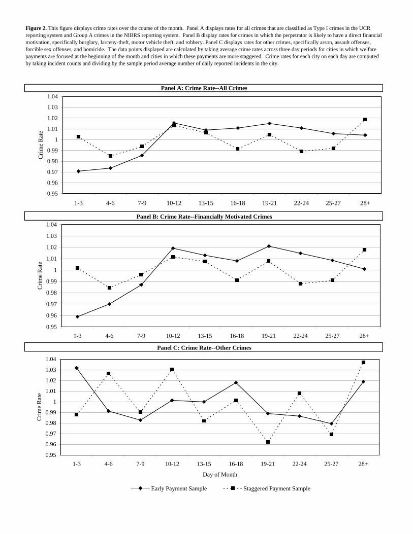
Figure 2 presents crime rates, averaged over three day intervals for the Early
Payment Sample and the Staggered Payment Sample. Daily crime rates are computed for
each city and type of crime by dividing the count of reported incidents by the sample
period average number of reported incidents in the city.12 Panel A displays rates for all
crimes. The solid line with diamond markers indicates how rates change over the course
of the month in cities in the Early Payment Sample. Rates increase from around 0.97 at
the start of the month to more than 1.01 by the middle of the month, implying an increase
in the crime rate for all types of crime of about 4%. The number of reported incidents
stays above average until the end of the month. Panel B and C respectively show crime
rates for financially motivated crimes and non-financially motivated crimes. In cities in
the Early Payment Sample, there are pronounced increases in financially motivated
crimes but no discernable trend in other crimes. Financially motivated crime rates
11 For each city, weather measurements are taken from the airport station nearest to the city and missing data are augmented with data from other nearby stations. 12 Jacob, Lefgren, and Morretti (forthcoming) use a similar approach to measure weekly crime rates.

15
increase from around 0.96 at the beginning of the month to more than 1.02 by the 19th to
the 21st of the month, indicating an increase of about 6%.
The dotted lines with square markers indicate how crime rates change over the
course of the month for cities in the Staggered Payment Sample. In this sample, there is
no apparent trend in overall crime, financially motivated crime, or other crime over the
course of the month. These patterns in Figure 1 are consistent with the theory that
welfare beneficiaries exhaust their welfare related income soon after receiving it and then
attempt to augment their income with income from criminal activity later in the month.
Patterns in crime observed in the Early Payment Sample do not seem to be a consequence
of factors that are also operative in the Staggered Payment Sample.
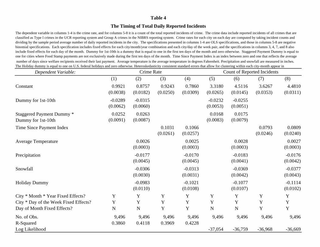
Table 4 presents the results of specifications that analyze patterns in total reported
incidents of Type I or Group A crimes. The dependent variable studied in the OLS
specifications in columns 1-4 is the crime rate, which is defined as the number of
reported incidents in a city on a particular date divided by average daily reported
incidents in the city. Each specification in Table 4 includes two kinds of fixed effects.13
City*Month*Year fixed effects control for differences across cities even if these vary
month to month. City*Day of Week fixed effects control for differences in criminal
activity across days of the week in individual cities. The coefficients on Dummy for 1st-
10th are negative and significant in columns 1 and 2. The -0.0315 coefficient in column 2
implies that the crime rate is 3.2% below average during the first ten days of the month in
cities where welfare payments are focused in the beginning of the month. The
coefficients on the Staggered Payment Dummy interacted with the Dummy for 1st-10th
13 The results in Table 4 and the remainder of the analysis do not appear to depend on the inclusion of these fixed effects. Using only city fixed effects to control for constant city characteristics yields estimates of the effects of the timing of welfare payments on crime that are similar to those presented in Tables 4-8.

16
are positive and significant and of slightly smaller magnitude than the coefficients on the
Dummy for 1st-10th. An F-test reveals that the sum of the coefficients on Dummy for 1st-
10th and on the interaction terms for each specification is not statistically distinguishable
from zero. These results indicate that there are no discernable increases in reported
incidents of crime in cities in the Staggered Payment sample. Factors that are operative
in both the Early Payment sample and the Staggered Payment sample, like the convention
that rents are due at the start of the month, do not explain increases in crime in the Early
Payment sample.
The specifications in column 2 include controls for weather and a dummy that is
equal to one on holidays and zero otherwise. Consistent with previous work, crime
appears to increase as temperatures rise and decrease with precipitation and snowfall.
Crime rates are also lower on holidays.
The specifications presented in columns 3 and 4 include the Time Since Payment
Index instead of the dummy capturing the time within the month and the timing of
welfare payments. These specifications also include a fixed effect for each calendar day
of the month so the coefficient on the index is identified off of differences in the timing
and frequency of welfare payments across cities. The results indicate that crime rates
increase with the amount of time that has passed since welfare payments occurred. The
0.1066 coefficient on the Time Since Payment Index in column 4 implies that, if all
welfare payments occurred on the first of the month, crime rates would be 10.7% higher
on the 31st of the month relative to the 1st of the month.
Columns 5-8 of Table 4 contain results of negative binomial specifications that
analyze counts of reported incidents as opposed to crime rates. The results in the
17
specifications are qualitatively and quantitatively very similar to those in columns 1-4.
These findings are consistent with the hypothesis that criminal income supplements
welfare income at the end of monthly welfare payment cycles.
The timing of welfare payments is hypothesized to affect crimes in which
perpetrators have a direct financial motivation and not necessarily other kinds of crime.
The specifications in Table 5 analyze crimes that are likely to have financial motives.
The specifications in this table are the same as those presented in Table 4 except the
dependent variables analyzed are the rate of financially motivated crime in columns 1-4
and the count of reported incidents of financially motivated crime in columns 5-8. As in
Table 4, the coefficients on the Dummy for 1st-10th are negative and significant and the
coefficients on this dummy interacted with the Staggered Payment Dummy are positive
and significant. These results indicate that there are increases in financially motivated
crimes in cities where welfare payments are focused at the beginning of the month. In
cities where welfare payments are more staggered, increases are less pronounced and do
not differ statistically from the null of there being no temporal trend. The coefficients on
the Time Since Payment Index are also positive and significant.
The effects of the timing of welfare payments on financially motivated crimes
appear to be more pronounced than its effects on total crime analyzed in Table 4. The -
0.0371 coefficient on the Dummy for 1st-10th in column 2 implies that, in the Early
Payment Sample, the financially motivated crime rate is 3.7% (as opposed to 3.1% for all
crimes) below average in the first 10 days of the month than it is over the rest of the
month. The 0.1227 coefficient on Day of the Month in column 4 indicates that the
financially motivated crime rate is 12.7% (as opposed to 10.7% for all crimes) higher on
18
the 31st of the month relate to the 1st in a city where all welfare payments occur on the 1st
of the month.
If patterns in crime reflect reporting biases or effects of police deployment that
are similar across different types of crime, then the data would indicate an increase in
non-financially motivated crimes over the course of welfare payment cycles as well. The
hypothesis that patterns in crime reflect income needs that arise during welfare payment
cycles does not make this prediction about non-financially motivated crimes. Table 6
presents results of specifications that test for temporal trends in non-financially motivated
crimes; these include arson, assault offenses, forcible sex offenses, and homicide. These
specifications are the same as those presented in Tables 4 and 5, but the dependent
variables considered are the non-financially motivated crime rate in columns 1-4 and the
count of reported incidents of non-financially motivated crime in columns 5-8. The
results do not include any statistically significant relations between the timing of welfare
payments and non-financially motivated crimes. The coefficients on the Dummy for 1st-
10th are positive, but they are insignificant and of much smaller magnitude than the
coefficients on this variable in the specifications that explain financially motivated crimes
presented in Table 5. The coefficients on the Time Since Payment Index are also
insignificant. These results suggest that explanations for patterns in crime over monthly
welfare payment cycles that do not differentiate between financially motivated and other
crimes are incomplete.
As mentioned in Section II, the distinction between the Early Payment Sample
and the Staggered Payment Sample used in the tests that include the dummy that is equal
to one for the first ten days of the month is subject to some concerns. This distinction is
19
based on the timing of Food Stamp payments. While this form of welfare is the largest
one in terms of the number of recipients, TANF programs are larger in value terms in
many jurisdictions. The timing of payments in these programs differs from the timing of
Food Stamp payments. In order to confirm that results are robust to using a more strictly
defined sample, I drop Detroit, MI, Philadelphia, PA, Providence, RI, and Milwaukee,
WI from the sample. These are cities in which either Food Stamp payments are focused
at the beginning of the month but TANF payments are more staggered or Food Stamp
payments are staggered but TANF payments are focused at the beginning of the month.14
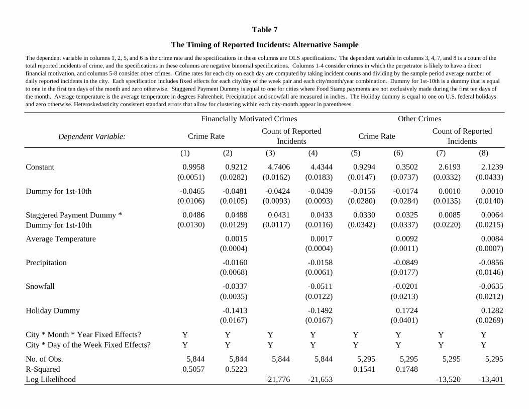
The results of some of the specifications presented in Tables 5 and 6, but run
using the reduced sample, appear in Table 7. Columns 1-4 and 5-8 respectively contain
specifications that analyze financially motivated and other crimes. For each type of
crime, the dependent variable in the first two specifications is the crime rate, and it is the
count of reported incidents in the second two specifications.
The results indicate that using the more strictly defined sample yields estimates
suggesting larger effects of the timing of welfare payments. The coefficients on the
Dummy for 1st-10th are larger in magnitude than the coefficients on this variables in the
specifications presented in Table 5 that analyze the full sample of cities. The interaction
terms including the Staggered Payment Dummy are also of larger magnitude. The
estimates in column 2 imply that in the more strictly defined Early Payment Sample,
financially motivated crime rates are 4.8% lower during the first ten days of the month
than they are during the remainder of the month. The results in columns 5-8 indicate that
14 In this robustness check, I do not drop New Orleans. Food Stamp payments occur during the 5th-14th period and family assistance payments occur from the 1st-5th. This payment schedule is consistent with including this city in the Staggered Payment Sample. Removing it does not qualitatively or quantitatively change the results in a significant way.
20
there are no significant temporal patterns in non-financially motivated crimes in either the
strictly defined Early Payment Sample or Staggered Payment Sample.
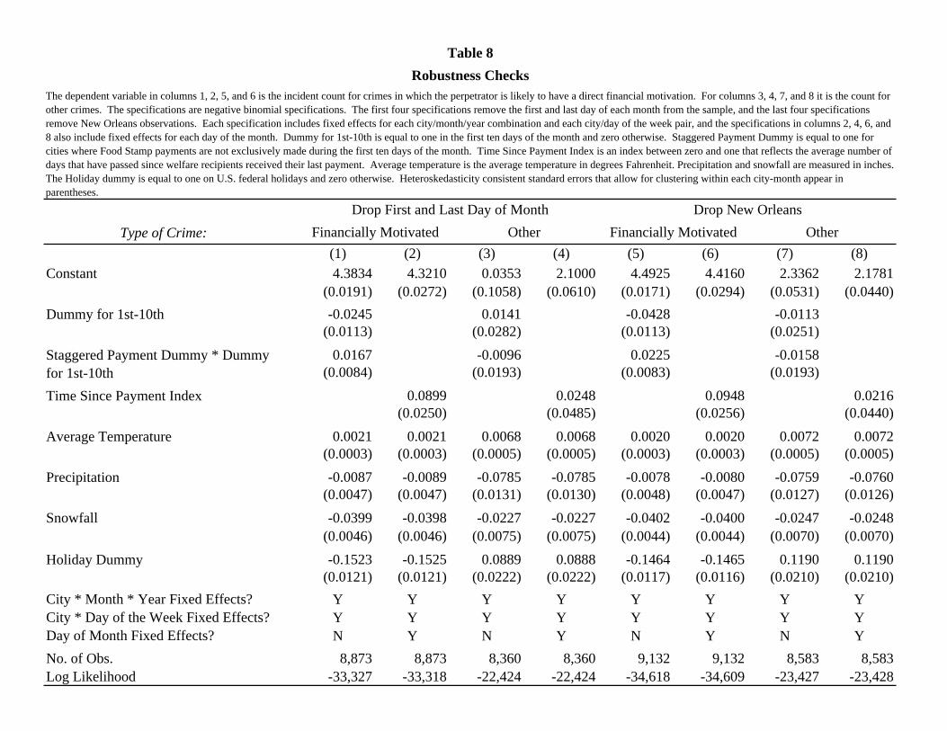
Table 8 presents results of two other robustness checks. First, measurement error
could give rise to an excessive number of reported incidents on the first or last day of the
month. For example, if there is a delay between when a crime occurs and when it is
discovered or reported, there may be an incentive to report the crime on the first or last
day of the month so it is included in crime statistics for that month. The specifications
presented in columns 1-4 of Table 8 test if the results are robust to this kind of error by
dropping observations from the first and last day of the month. The specifications
analyze financially motivated crime rates in columns 1-2 and other crime rates in
columns 3-4. The results are little changed by this adjustment to the sample. As a
second additional robustness check, the specifications in columns 5-8 of Table 8 drop
New Orleans from the sample. The New Orleans data only cover 2006 and conflating
factors related to the aftermath of hurricane Katrina could affect patterns of crime in the
city. The results indicate that removing New Orleans from the sample does not
substantively change the results.
5. Conclusion
Analysis of patterns in crime in 12 large U.S. cities where more than 10% of the
population receive welfare benefits indicates that the timing of welfare payments affects
criminal activity. More crime occurs when more time has passed since welfare payments
occurred. This finding is consistent with the hypothesis that individuals who receive
support from welfare payments consume their benefits quickly and then attempt to
21
supplement these payments with income from criminal activity. The increase reflects an
increase in crimes in which the perpetrator is likely to have a direct financial motivation
and not other types of Part I UCR or Group A NIBRS offenses. Temporal patterns in
crime are not observed in jurisdictions where welfare payments are more staggered.
These additional results rule out many other potential explanations for monthly patterns
in crime.
These findings have implications for the design of welfare programs. Increasing
the frequency of welfare payments would be likely to diminish temporal patterns in
crime. The results suggest that frequent payments that are sufficiently large would be
associated with lower levels of crime. Furthermore, if criminal activity were smoothed
over time, it might be easier to combat. Nearly all jurisdictions now distribute Food
Stamp payments and family assistance payments on electronic benefit transfer cards, so
the costs of more frequent payments would be likely to be low. Shaprio (2005), Wilde
and Ranney (2000), and Ohls, Fraker, Martini, and Ponza (1992) also present arguments
in favor of more frequent payments. These suggestions are in line with calls to
incorporate behavior considerations into public policy, like those in Jolls (2007) and
Bertrand, Mullainathan, and Shafir (2004).
These findings also have implications for the deployment of police officers and
the labor laws applicable to law enforcement. In jurisdictions where welfare payments
are focused at the beginning of the month, increased levels of criminal activity at the end
of the month call for more police protection during this time. However, 1986
amendments to the Fair Labor Standards Act require that law enforcement officers be
compensated for working more than 40 hours a week. As a consequence, it is costly for
22
departments to shift resources to times when they are particularly needed. More flexible
labor law could help fight crime.
23
References
Angeletos, George-Marios, David Laibson, Andrea Repetto, Jeremy Tobacman, and Stephen Weinberg, 2001, The Hyperbolic Consumption Model: Calibration, Simulation, and Empirical Evaluation, Journal of Economic Perspectives 15:3, pp. 47-68.
Barr, Michael, 2004, Banking the Poor, Yale Journal of Regulation 21, pp. 121-237. Becker, Gary S., Crime and Punishment: An Economic Approach, Journal of Political
Economy 76:2, pp. 169-217. Bertrand, Marianne, Sendhil Mullainathan, and Eldar Shafir, 2004, A Behavior
Economics View of Poverty, American Economic Review 94:2, pp. 419-423. Beverly, Sondra, Daniel Shneider, and Peter Tufano, 2006, Splitting Tax Refunds and
Building Savings: An Empirical Test, Tax Policy and the Economy 20, pp. 111-161. Burek, Melissa, 2005, Now Serving Part Two Crimes: Testing the Relationship between
Welfare Spending and Property Crimes, Criminal Justice Policy Review 16:3, pp. 360-384.
Campbell, John, 2006, Household Finance, Journal of Finance 61, pp. 1553-1604. Cole, Nancy and Ellie Lee, 2005, An Analysis of EBT Benefit Redemption Patterns:
Methods for Obtaining, Preparing, and Analyzing the Data, Abt Associates, Inc. DeFranzo, James, 1996, Welfare and Burglary, Crime and Delinquency 42, pp 223-229. DeFranzo, James, 1997, Welfare and Homicide, Journal of Research in Crime and
Delinquency 34, pp. 395-406. Dobkin, Carlos and Stephen Puller, forthcoming, The Effects of Government Transfers
on Monthly Cycles in Drug Abuse, Hospitalization, and Mortality, Journal of Public Economics.
Donohue, John, and Steven Levitt, 2001, The Impact of Legalized Abortion on Crime,
The Quarterly Journal of Economics 116:2, pp. 379-420. Duflo, Esther, William Gale, Jeffrey Liebman, Peter Orszag, and Emmanuel Saez,
Quarterly Journal of Economics 121:4, pp. 1311-1346. Fellowes, Matt and Alan Berube, 2005, Leaving Money (and Food) on the Table: Food
Stamp Participation in Major Metropolitan Areas and Counties, The Brookings Institution Survey Series.

24
Freeman, Richard, 1995, The Labor Market, in Crime, James Q. Wilson and Joan Petersilia eds., San Francisco: ICS Press, pp. 171-192.
Garmaise, Mark and Tobias Moskowitz, Bank Mergers and Crime: The Real and Social
Effects of Credit Market Competition, Journal of Finance 61:2, pp. 495-539. Gould, Eric D., Bruce A. Weinberg and David B. Mustard, 2002, Crime Rates and Local
Labor Market Opportunities in the United States: 1979-1997, The Review of Economics and Statistics 84:1, pp. 45-61.
Hannon, Lance and James DeFranzo, 1998a, Welfare and Property Crime, Justice
Quarterly 15, pp. 273-287. Hannon, Lance and James DeFranzo, 1998b, The Truly Disadvantaged, Public
Assistance, and Crime, Social Problems 45, pp. 432-445. Hseih, Chang-Tai, 2003, Do Consumers Respond to Anticipated Income Changes?
Evidence from the Alaska Permanent Fund, American Economic Review 93:1, pp. 397-405.
Jacob, Brian, and Lars Lefgren, 2003, Are Idle Hands the Devil’s Workshop?
Incapacitation, Concentration, and Juvenile Crime, American Economic Review 93:5, pp. 1560-1577.
Jacob, Brian, Lars Lefgren, and Enrico Morretti, forthcoming, The Dynamics of Criminal
Behavior: Evidence from Weather Shocks, Journal of Human Resources. Johnson, David S., Jonathan A. Parker, and Nicholas Souleles, 2006, Household
Expenditure and the Income Tax Rebates of 2001, American Economic Review 96:5, pp. 1589-1610.
Jolls, Christine, 2007, Behavioral Law and Economics, Yale Law School working paper. Laibson, David, 1997, Golden Eggs and Hyperbolic Discounting, Quarterly Journal of
Economics 112:2, pp. 443-477. Lee, David S., and Justin McCrary, 2005, Crime, Punishment and Myopia, NBER
Working Paper No. 11491. Machin, Stephen and Costas Meghir, 2004, Crime and Economic Incentives, The Journal
of Human Resources 39:4, pp. 958-979. Moffitt, Robert, 1992, Incentive Effects of the U.S. Welfare System, Journal of
Economic Literature 30:1, pp. 1-61.
25
O’Donohue, Ted, and Matthew Rabin, Doing it Now or Later, American Economic Review 89:1, pp. 103-124.
O’Donohue, Ted, and Matthew Rabin, Choice and Procrastination, Quarterly Journal of
Economics 116:1, pp. 121-160. Ohls, James C., Thomas M. Fraker, Alberto P. Martini, and Michael Ponza, 1992, The
Effect of Cash-Out on Food Stamp Use by Food Stamp Participants in San Diego, Mathmatica Policy Research, Inc.
Phelps, E. S. and R. A. Pollak, 1968, On Second-Best National Saving and Game-
Equilibrium Growth, The Review of Economic Studies 35:2, pp. 185-199. Raphael, Steven, and Rudolf Winter-Ember, Identifying the Effect of Unemployment on
Crime, Journal of Law and Economics, 44:1, pp. 259-283. Shapiro, Jesse, 2005, Is there a Daily Discount Rate? Evidence from the Food Stamp
Nutrition Cycle, Journal of Public Economics 89:2-3, pp. 303-325. Shapiro, Matthew, and Joel Slemrod, 2003, Consumer Reponse to Tax Rebates,
American Economic Review 93:1, pp. 381-396. Stephens, Melvin, 2003, “3rd of tha Month”: Do Social Security Recipients Smooth
Consumption between Checks?, American Economic Review 93:1, pp. 406-422. Wilde, Park E. and Christine K. Ranney, 2000, The Monthly Food Stamp Cycle:
Shopping Frequency and Food Intake Decisions in an Endogenous Switching Regression Framework, American Journal of Agricultural Economics 82:1, pp. 200-213.

Figure 1: This figure displays the values of the Time Since Payment Index for Providence and St. Louis for each day of the month. The Time Since Payment Index is an index between zero and one that reflects the average number of days that have passed since welfare recipients received their last payment. It accounts for payments related to Food Stamps, TANF, and SSI. If a program makes payments over a range of dates, it is assumed that an equal number of recipients receives payment on each day in the range. The total number of recipients in each program is used to weight the payment schedules of each program.
0
0.1
0.2
0.3
0.4
0.5
0.6
0.7
0.8
0.9
1 3 5 7 9 11 13 15 17 19 21 23 25 27 29 31
Day of Month
Tim
e Si
nce
Paym
ent I
ndex
Providence St. Louis
Panel A: Crime Rate--All Crimes
Panel B: Crime Rate--Financially Motivated Crimes
Panel C: Crime Rate--Other Crimes
Figure 2. This figure displays crime rates over the course of the month. Panel A displays rates for all crimes that are classified as Type I crimes in the UCR reporting system and Group A crimes in the NIBRS reporting system. Panel B display rates for crimes in which the perpetrator is likely to have a direct financial motivation, specifically burglary, larceny-theft, motor vehicle theft, and robbery. Panel C displays rates for other crimes, specifically arson, assault offenses, forcible sex offenses, and homicide. The data points displayed are calculated by taking average crime rates across three day periods for cities in which welfare payments are focused at the beginning of the month and cities in which these payments are more staggered. Crime rates for each city on each day are computed by taking incident counts and dividing by the sample period average number of daily reported incidents in the city.
0.95
0.96
0.97
0.98
0.99
1
1.01
1.02
1.03
1.04
1-3 4-6 7-9 10-12 13-15 16-18 19-21 22-24 25-27 28+
Crim
e R
ate
0.95
0.96
0.97
0.98
0.99
1
1.01
1.02
1.03
1.04
1-3 4-6 7-9 10-12 13-15 16-18 19-21 22-24 25-27 28+
Crim
e R
ate
0.95
0.96
0.97
0.98
0.99
1
1.01
1.02
1.03
1.04
1-3 4-6 7-9 10-12 13-15 16-18 19-21 22-24 25-27 28+
Day of Month
Crim
e R
ate
Early Payment Sample Staggered Payment Sample
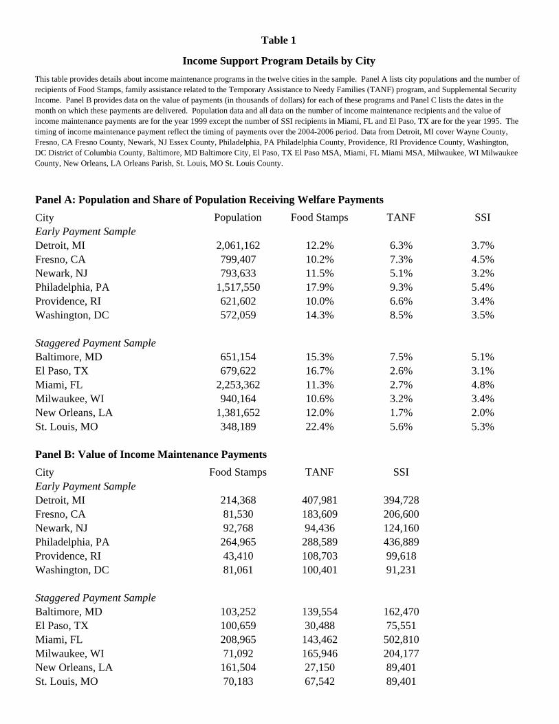
Panel A: Population and Share of Population Receiving Welfare PaymentsCity Population Food Stamps TANF SSIEarly Payment SampleDetroit, MI 2,061,162 12.2% 6.3% 3.7%Fresno, CA 799,407 10.2% 7.3% 4.5%Newark, NJ 793,633 11.5% 5.1% 3.2%Philadelphia, PA 1,517,550 17.9% 9.3% 5.4%Providence, RI 621,602 10.0% 6.6% 3.4%Washington, DC 572,059 14.3% 8.5% 3.5%
Staggered Payment SampleBaltimore, MD 651,154 15.3% 7.5% 5.1%El Paso, TX 679,622 16.7% 2.6% 3.1%Miami, FL 2,253,362 11.3% 2.7% 4.8%Milwaukee, WI 940,164 10.6% 3.2% 3.4%New Orleans, LA 1,381,652 12.0% 1.7% 2.0%St. Louis, MO 348,189 22.4% 5.6% 5.3%
Panel B: Value of Income Maintenance PaymentsCity Food Stamps TANF SSIEarly Payment SampleDetroit, MI 214,368 407,981 394,728Fresno, CA 81,530 183,609 206,600Newark, NJ 92,768 94,436 124,160Philadelphia, PA 264,965 288,589 436,889Providence, RI 43,410 108,703 99,618Washington, DC 81,061 100,401 91,231
Staggered Payment SampleBaltimore, MD 103,252 139,554 162,470El Paso, TX 100,659 30,488 75,551Miami, FL 208,965 143,462 502,810Milwaukee, WI 71,092 165,946 204,177New Orleans, LA 161,504 27,150 89,401St. Louis, MO 70,183 67,542 89,401
Table 1
Income Support Program Details by CityThis table provides details about income maintenance programs in the twelve cities in the sample. Panel A lists city populations and the number of recipients of Food Stamps, family assistance related to the Temporary Assistance to Needy Families (TANF) program, and Supplemental Security Income. Panel B provides data on the value of payments (in thousands of dollars) for each of these programs and Panel C lists the dates in the month on which these payments are delivered. Population data and all data on the number of income maintenance recipients and the value of income maintenance payments are for the year 1999 except the number of SSI recipients in Miami, FL and El Paso, TX are for the year 1995. The timing of income maintenance payment reflect the timing of payments over the 2004-2006 period. Data from Detroit, MI cover Wayne County, Fresno, CA Fresno County, Newark, NJ Essex County, Philadelphia, PA Philadelphia County, Providence, RI Providence County, Washington, DC District of Columbia County, Baltimore, MD Baltimore City, El Paso, TX El Paso MSA, Miami, FL Miami MSA, Milwaukee, WI Milwaukee County, New Orleans, LA Orleans Parish, St. Louis, MO St. Louis County.
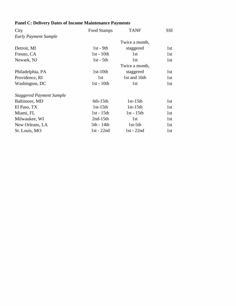
Panel C: Delivery Dates of Income Maintenance PaymentsCity Food Stamps TANF SSIEarly Payment Sample
Detroit, MI 1st - 9thTwice a month,
staggered 1stFresno, CA 1st - 10th 1st 1stNewark, NJ 1st - 5th 1st 1st
Philadelphia, PA 1st-10thTwice a month,
staggered 1stProvidence, RI 1st 1st and 16th 1stWashington, DC 1st - 10th 1st 1st
Staggered Payment SampleBaltimore, MD 6th-15th 1st-15th 1stEl Paso, TX 1st-15th 1st-15th 1stMiami, FL 1st - 15th 1st - 15th 1stMilwaukee, WI 2nd-15th 1st 1stNew Orleans, LA 5th - 14th 1st-5th 1stSt. Louis, MO 1st - 22nd 1st - 22nd 1st
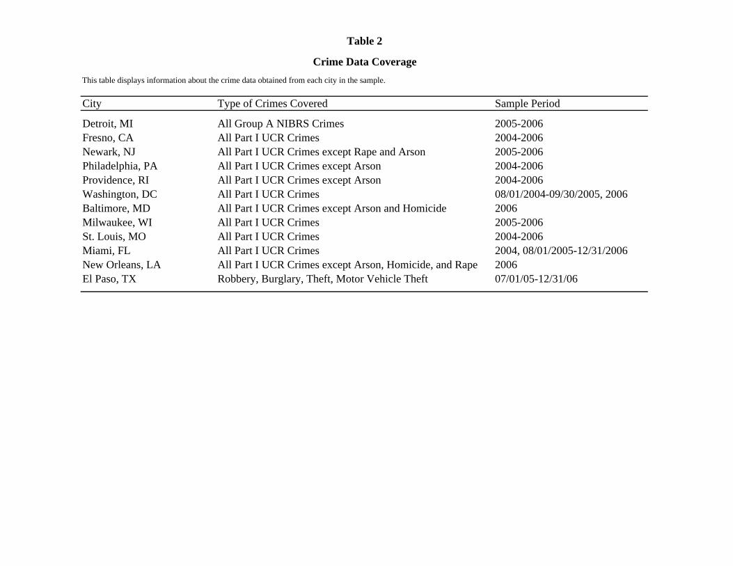
City Type of Crimes Covered Sample Period
Detroit, MI All Group A NIBRS Crimes 2005-2006Fresno, CA All Part I UCR Crimes 2004-2006Newark, NJ All Part I UCR Crimes except Rape and Arson 2005-2006Philadelphia, PA All Part I UCR Crimes except Arson 2004-2006Providence, RI All Part I UCR Crimes except Arson 2004-2006Washington, DC All Part I UCR Crimes 08/01/2004-09/30/2005, 2006Baltimore, MD All Part I UCR Crimes except Arson and Homicide 2006Milwaukee, WI All Part I UCR Crimes 2005-2006St. Louis, MO All Part I UCR Crimes 2004-2006Miami, FL All Part I UCR Crimes 2004, 08/01/2005-12/31/2006New Orleans, LA All Part I UCR Crimes except Arson, Homicide, and Rape 2006El Paso, TX Robbery, Burglary, Theft, Motor Vehicle Theft 07/01/05-12/31/06
Table 2
Crime Data CoverageThis table displays information about the crime data obtained from each city in the sample.

Mean MedianStandard Deviation
Crime Rate--All Crimes 1.000 0.998 0.182Count of Reported Incidents--All Crimes 107.690 96.000 66.038Crime Rate--Financially Motivated Crimes 1.000 0.995 0.215Count of Reported Incidents--Financially Motivated Crimes 91.604 75.000 60.061Crime Rate--Other Crimes 1.000 0.926 0.539Count of Reported Incidents--Other Crimes 15.642 12.000 12.132
Dummy for 1st-10th 0.329 0.000 0.470
Time Since Payment Index 0.470 0.455 0.178
Average Temperature 59.802 62.000 17.9300.108 0.000 0.342
Snowfall 0.051 0.000 0.504Holiday Dummy 0.032 0.000 0.176
Precipitation
Table 3Descriptive Statistics
The crime data include reported incidents of all crimes that are classified as Type I crimes in the UCR reporting system and Group A crimes in the NIBRS reporting system. Financially motivated crimes include reported incidents of crimes in which the perpetrator is likely to have a direct financial motivation, specifically burglary, larceny-theft, motor vehicle theft, and robbery. Other crimes include arson, assault offenses, forcible sex offenses, and homicide. Crime rates for each city on each day are computed by taking incident counts and dividing by the sample period average number of daily reported incidents in the city. Dummy for 1st-10th is a dummy that is equal to one in the first ten days of the month and zero otherwise. Time Since Payment Index is an index between zero and one that reflects the average number of days that have passed since welfare recipients received their last payment. Average temperature is the average temperature in degrees Fahrenheit. Precipitation and snowfall are measured in inches. The Holiday dummy is equal to one on U.S. federal holidays and zero otherwise.
Dependent Variable:(1) (2) (3) (4) (5) (6) (7) (8)
Constant 0.9921 0.8757 0.9243 0.7860 3.3180 4.5116 3.6267 4.4810(0.0038) (0.0182) (0.0250) (0.0309) (0.0265) (0.0145) (0.0353) (0.0311)
Dummy for 1st-10th -0.0289 -0.0315 -0.0232 -0.0255(0.0062) (0.0060) (0.0053) (0.0051)
0.0252 0.0263 0.0168 0.0175(0.0091) (0.0087) (0.0083) (0.0079)
Time Since Payment Index 0.1031 0.1066 0.0793 0.0809(0.0261) (0.0257) (0.0246) (0.0240)
Average Temperature 0.0026 0.0025 0.0028 0.0027(0.0003) (0.0003) (0.0003) (0.0003)-0.0177 -0.0170 -0.0183 -0.0176
(0.0045) (0.0045) (0.0041) (0.0042)Snowfall -0.0306 -0.0313 -0.0369 -0.0377
(0.0030) (0.0031) (0.0042) (0.0043)Holiday Dummy -0.0983 -0.1021 -0.1077 -0.1114
(0.0110) (0.0108) (0.0107) (0.0102)City * Month * Year Fixed Effects? Y Y Y Y Y Y Y YCity * Day of the Week Fixed Effects? Y Y Y Y Y Y Y YDay of Month Fixed Effects? N N Y Y N N Y Y
No. of Obs. 9,496 9,496 9,496 9,496 9,496 9,496 9,496 9,496R-Squared 0.3860 0.4118 0.3969 0.4228Log Likelihood -37,054 -36,759 -36,968 -36,669
Crime Rate Count of Reported Incidents
Staggered Payment Dummy * Dummy for 1st-10th
Precipitation
Table 4
The Timing of Total Daily Reported IncidentsThe dependent variable in columns 1-4 is the crime rate, and for columns 5-8 it is a count of the total reported incidents of crime. The crime data include reported incidents of all crimes that are classified as Type I crimes in the UCR reporting system and Group A crimes in the NIBRS reporting system. Crime rates for each city on each day are computed by taking incident counts and dividing by the sample period average number of daily reported incidents in the city. The specifications presented in columns 1-4 are OLS specifications, and those in columns 5-8 are negative binomial specifications. Each specification includes fixed effects for each city/month/year combination and each city/day of the week pair, and the specifications in columns 3, 4, 7, and 8 also include fixed effects for each day of the month. Dummy for 1st-10th is a dummy that is equal to one in the first ten days of the month and zero otherwise. Staggered Payment Dummy is equal to one for cities where Food Stamp payments are not exclusively made during the first ten days of the month. Time Since Payment Index is an index between zero and one that reflects the average number of days since welfare recipients received their last payment. Average temperature is the average temperature in degrees Fahrenheit. Precipitation and snowfall are measured in inches. The Holiday dummy is equal to one on U.S. federal holidays and zero otherwise. Heteroskedasticity consistent standard errors that allow for clustering within each city-month appear in

Dependent Variable:(1) (2) (3) (4) (5) (6) (7) (8)
Constant 1.0024 0.9332 0.9112 0.8145 3.2596 4.4193 3.5609 4.3772(0.0042) (0.0204) (0.0265) (0.0340) (0.0286) (0.0147) (0.0376) (0.0324)
Dummy for 1st-10th -0.0347 -0.0371 -0.0298 -0.0319(0.0065) (0.0063) (0.0054) (0.0051)
0.0308 0.0319 0.0237 0.0246(0.0096) (0.0093) (0.0088) (0.0083)
Time Since Payment 0.1199 0.1227 0.0965 0.0980(0.0278) (0.0275) (0.0258) (0.0252)
Average Temperature 0.0019 0.0018 0.0021 0.0020(0.0003) (0.0003) (0.0003) (0.0003)-0.0086 -0.0078 -0.0100 -0.0093
(0.0054) (0.0054) (0.0046) (0.0046)Snowfall -0.0320 -0.0328 -0.0391 -0.0399
(0.0026) (0.0026) (0.0044) (0.0044)Holiday Dummy -0.1372 -0.1411 -0.1459 -0.1496
(0.0124) (0.0124) (0.0119) (0.0115)City * Month * Year Fixed Effects? Y Y Y Y Y Y Y YCity * Day of the Week Fixed Effects? Y Y Y Y Y Y Y YDay of Month Fixed Effects? N N Y Y N N Y YNo. of Obs. 9,496 9,496 9,496 9,496 9,496 9,496 9,496 9,496R-Squared 0.4720 0.4928 0.4803 0.5012Log Likelihood -36,181 -35,907 -36,106 -35,828
Precipitation
Count of Reported Incidents
Staggered Payment Dummy * Dummy for 1st-10th
Table 5The Timing of Total Daily Reported Incidents--Financially Motivated Crimes
The dependent variable in columns 1-4 is the crime rate, and for columns 5-8 it is a count of the total reported incidents of crime. The crime data include reported incidents of crimes in which the perpetrator is likely to have a direct financial motivation, specifically burglary, larceny-theft, motor vehicle theft, and robbery. Crime rates for each city on each day are computed by taking incident counts and dividing by the sample period average number of daily reported incidents in the city. The specifications presented in columns 1-4 are OLS specifications, and those in columns 5-8 are negative binomial specifications. Each specification includes fixed effects for each city/month/year combination and each city/day of the week pair, and the specifications in columns 3, 4, 7, and 8 also include fixed effects for each day of the month. Dummy for 1st-10th is a dummy that is equal to one in the first ten days of the month and zero otherwise. Staggered Payment Dummy is equal to one for cities where Food Stamp payments are not exclusively made during the first ten days of the month. Time Since Payment Index is an index between zero and one that reflects the average number of days since welfare recipients received their last payment. Average temperature is the average temperature in degrees Fahrenheit. Precipitation and
Crime Rate
snowfall are measured in inches. The Holiday dummy is equal to one on U.S. federal holidays and zero otherwise. Heteroskedasticity consistent standard errors that allow for clustering within each city-month appear in parentheses.

Dependent Variable:(1) (2) (3) (4) (5) (6) (7) (8)
Constant 0.9191 0.4605 0.8941 0.4026 2.5702 0.5678 0.5499 0.6098(0.0110) (0.0448) (0.0612) (0.0751) (0.0460) (0.1054) (0.1067) (0.1131)
Dummy for 1st-10th 0.0061 0.0023 0.0132 0.0108(0.0196) (0.0197) (0.0145) (0.0141)
0.0027 0.0046 -0.0145 -0.0141(0.0253) (0.0248) (0.0197) (0.0191)
Time Since Payment Index 0.0785 0.0894 0.0185 0.0263(0.0650) (0.0635) (0.0455) (0.0435)
Average Temperature 0.0080 0.0079 0.0074 0.0072(0.0007) (0.0007) (0.0005) (0.0005)-0.0828 -0.0819 -0.0766 -0.0758
(0.0128) (0.0129) (0.0124) (0.0125)Snowfall -0.0213 -0.0215 -0.0241 -0.0248
(0.0094) (0.0097) (0.0068) (0.0070)Holiday Dummy 0.1547 0.1468 0.1291 0.1219
(0.0276) (0.0271) (0.0207) (0.0210)City * Month * Year Fixed Effects? Y Y Y Y Y Y Y YCity * Day of the Week Fixed Effects? Y Y Y Y Y Y Y YDay of Month Fixed Effects? N N Y Y N N Y Y
No. of Obs. 8,947 8,947 8,947 8,947 8,947 8,947 8,947 8,947R-Squared 0.4195 0.4352 0.4226 0.4372Log Likelihood -24,289 -24,097 -24,257 -24,077
Table 6The Timing of Total Daily Reported Incidents--Other Crimes
The dependent variable in columns 1-4 is the crime rate, and for columns 5-8 it is a count of the total reported incidents of crime. The crime data include reported incidents of arson, assault offenses, forcible sex offenses, and homicide. Crime rates for each city on each day are computed by taking incident counts and dividing by the sample period average number of daily reported incidents in the city. The specifications presented in columns 1-4 are OLS specifications, and those in columns 5-8 are negative binomial specifications. Each specification includes fixed effects for each city/month/year combination and each city/day of the week pair, and the specifications in columns 3, 4, 7, and 8 also include fixed effects for each day of the month. Dummy for 1st-10th is a dummy that is equal to one in the first ten days of the month and zero otherwise. Staggered Payment Dummy is equal to one for cities where Food Stamp payments are not exclusively made during the first ten days of the month. Time Since Payment Index is an index between zero and one that reflects the average number of days that have passed since welfare recipients received their last payment. Average temperature is the average temperature in degrees Fahrenheit. Precipitation and snowfall are measured in inches. The Holiday dummy is equal to one on U.S. federal holidays and zero otherwise. Heteroskedasticity consistent standard errors that allow for clustering within each city-month appear in parentheses.
Precipitation
Crime Rate Count of Reported Incidents
Staggered Payment Dummy * Dummy for 1st-10th
Dependent Variable:
(1) (2) (3) (4) (5) (6) (7) (8)
Constant 0.9958 0.9212 4.7406 4.4344 0.9294 0.3502 2.6193 2.1239(0.0051) (0.0282) (0.0162) (0.0183) (0.0147) (0.0737) (0.0332) (0.0433)
Dummy for 1st-10th -0.0465 -0.0481 -0.0424 -0.0439 -0.0156 -0.0174 0.0010 0.0010(0.0106) (0.0105) (0.0093) (0.0093) (0.0280) (0.0284) (0.0135) (0.0140)
0.0486 0.0488 0.0431 0.0433 0.0330 0.0325 0.0085 0.0064(0.0130) (0.0129) (0.0117) (0.0116) (0.0342) (0.0337) (0.0220) (0.0215)
Average Temperature 0.0015 0.0017 0.0092 0.0084(0.0004) (0.0004) (0.0011) (0.0007)
-0.0160 -0.0158 -0.0849 -0.0856(0.0068) (0.0061) (0.0177) (0.0146)
Snowfall -0.0337 -0.0511 -0.0201 -0.0635(0.0035) (0.0122) (0.0213) (0.0212)
Holiday Dummy -0.1413 -0.1492 0.1724 0.1282(0.0167) (0.0167) (0.0401) (0.0269)
City * Month * Year Fixed Effects? Y Y Y Y Y Y Y YCity * Day of the Week Fixed Effects? Y Y Y Y Y Y Y Y
No. of Obs. 5,844 5,844 5,844 5,844 5,295 5,295 5,295 5,295R-Squared 0.5057 0.5223 0.1541 0.1748Log Likelihood -21,776 -21,653 -13,520 -13,401
Staggered Payment Dummy * Dummy for 1st-10th
Precipitation
Financially Motivated Crimes Other Crimes
Crime Rate Count of Reported Incidents Crime Rate Count of Reported
Incidents
Table 7
The Timing of Reported Incidents: Alternative SampleThe dependent variable in columns 1, 2, 5, and 6 is the crime rate and the specifications in these columns are OLS specifications. The dependent variable in columns 3, 4, 7, and 8 is a count of the total reported incidents of crime, and the specifications in these columns are negative binomial specifications. Columns 1-4 consider crimes in which the perpetrator is likely to have a direct financial motivation, and columns 5-8 consider other crimes. Crime rates for each city on each day are computed by taking incident counts and dividing by the sample period average number of daily reported incidents in the city. Each specification includes fixed effects for each city/day of the week pair and each city/month/year combination. Dummy for 1st-10th is a dummy that is equal to one in the first ten days of the month and zero otherwise. Staggered Payment Dummy is equal to one for cities where Food Stamp payments are not exclusively made during the first ten days of the month. Average temperature is the average temperature in degrees Fahrenheit. Precipitation and snowfall are measured in inches. The Holiday dummy is equal to one on U.S. federal holidays and zero otherwise. Heteroskedasticity consistent standard errors that allow for clustering within each city-month appear in parentheses.
Type of Crime:(1) (2) (3) (4) (5) (6) (7) (8)
Constant 4.3834 4.3210 0.0353 2.1000 4.4925 4.4160 2.3362 2.1781(0.0191) (0.0272) (0.1058) (0.0610) (0.0171) (0.0294) (0.0531) (0.0440)
Dummy for 1st-10th -0.0245 0.0141 -0.0428 -0.0113(0.0113) (0.0282) (0.0113) (0.0251)
0.0167 -0.0096 0.0225 -0.0158(0.0084) (0.0193) (0.0083) (0.0193)
Time Since Payment Index 0.0899 0.0248 0.0948 0.0216(0.0250) (0.0485) (0.0256) (0.0440)
Average Temperature 0.0021 0.0021 0.0068 0.0068 0.0020 0.0020 0.0072 0.0072(0.0003) (0.0003) (0.0005) (0.0005) (0.0003) (0.0003) (0.0005) (0.0005)-0.0087 -0.0089 -0.0785 -0.0785 -0.0078 -0.0080 -0.0759 -0.0760
(0.0047) (0.0047) (0.0131) (0.0130) (0.0048) (0.0047) (0.0127) (0.0126)Snowfall -0.0399 -0.0398 -0.0227 -0.0227 -0.0402 -0.0400 -0.0247 -0.0248
(0.0046) (0.0046) (0.0075) (0.0075) (0.0044) (0.0044) (0.0070) (0.0070)Holiday Dummy -0.1523 -0.1525 0.0889 0.0888 -0.1464 -0.1465 0.1190 0.1190
(0.0121) (0.0121) (0.0222) (0.0222) (0.0117) (0.0116) (0.0210) (0.0210)City * Month * Year Fixed Effects? Y Y Y Y Y Y Y YCity * Day of the Week Fixed Effects? Y Y Y Y Y Y Y YDay of Month Fixed Effects? N Y N Y N Y N YNo. of Obs. 8,873 8,873 8,360 8,360 9,132 9,132 8,583 8,583Log Likelihood -33,327 -33,318 -22,424 -22,424 -34,618 -34,609 -23,427 -23,428
Precipitation
Drop First and Last Day of Month Drop New OrleansFinancially Motivated Other Financially Motivated Other
Table 8Robustness Checks
The dependent variable in columns 1, 2, 5, and 6 is the incident count for crimes in which the perpetrator is likely to have a direct financial motivation. For columns 3, 4, 7, and 8 it is the count for other crimes. The specifications are negative binomial specifications. The first four specifications remove the first and last day of each month from the sample, and the last four specifications remove New Orleans observations. Each specification includes fixed effects for each city/month/year combination and each city/day of the week pair, and the specifications in columns 2, 4, 6, and 8 also include fixed effects for each day of the month. Dummy for 1st-10th is equal to one in the first ten days of the month and zero otherwise. Staggered Payment Dummy is equal to one for cities where Food Stamp payments are not exclusively made during the first ten days of the month. Time Since Payment Index is an index between zero and one that reflects the average number of days that have passed since welfare recipients received their last payment. Average temperature is the average temperature in degrees Fahrenheit. Precipitation and snowfall are measured in inches. The Holiday dummy is equal to one on U.S. federal holidays and zero otherwise. Heteroskedasticity consistent standard errors that allow for clustering within each city-month appear in
Staggered Payment Dummy * Dummy for 1st-10th
parentheses.

City 1999 2000 2001 2002 2003 2004 2005Early Payment SampleDetroit, MI 214,368 184,614 198,103 228,424 278,983 313,485 373,735Fresno, CA 81,530 77,333 77,210 84,075 91,431 107,505 130,202Newark, NJ 92,768 81,240 75,459 73,506 77,060 85,071 95,870Philadelphia, PA 264,965 242,318 236,811 244,870 405,520 303,778 337,227Providence, RI 43,410 44,259 45,302 48,556 53,067 56,693 59,613Washington, DC 81,061 74,875 70,862 77,074 95,185 96,825 103,176
Staggered Payment SampleBaltimore, MD 103,252 94,394 94,263 97,190 108,055 119,352 131,438El Paso, TX 100,659 95,164 99,027 111,226 140,900 170,434 198,981Miami, FL 208,965 229,338 230,999 246,204 270,005 371,997 424,516Milwaukee, WI 71,092 74,277 86,645 102,435 117,257 136,054 157,348New Orleans, LA 101,959 95,955 104,774 119,186 121,294 133,431 235,945St. Louis, MO 70,183 71,939 78,095 85,815 96,768 110,754 118,428
1999 2000 2001 2002 2003 2004 2005Early Payment SampleDetroit, MI 407,981 413,728 353,028 365,952 349,953 340,491 332,969Fresno, CA 183,609 202,885 195,583 181,232 194,390 203,000 196,871Newark, NJ 94,436 84,603 105,935 106,050 114,466 109,579 97,639Philadelphia, PA 288,589 403,194 237,214 247,132 245,940 273,650 283,211Providence, RI 108,703 110,766 106,010 108,097 101,959 101,527 109,847Washington, DC 100,401 110,064 118,644 129,304 119,402 118,165 115,150
Staggered Payment SampleBaltimore, MD 139,554 149,623 140,844 126,662 105,860 134,910 146,929El Paso, TX 30,488 32,188 31,760 30,065 34,753 28,565 29,784Miami, FL 143,462 157,218 163,535 150,467 130,201 125,873 110,398Milwaukee, WI 165,946 219,813 271,941 280,726 293,403 307,476 287,444New Orleans, LA 27,150 26,746 30,240 33,358 27,437 23,912 20,869St. Louis, MO 67,542 70,109 70,747 63,650 37,134 37,839 34,890
Welfare Program Details by City
Appendix Table 1
Food Stamps
TANF
This table displays the value of welfare program payments (in thousands of dollars) over the 1999-2005 period. Data from Detroit, MI cover Wayne County, Fresno, CA Fresno County, Newark, NJ Essex County, Philadelphia, PA, Philadelphia County, Providence, RI Providence County, Washington, DC District of Columbia County, Baltimore, MD, Baltimore City, El Paso, TX, El Paso MSA, Miami, FL, Miami MSA, Milwaukee, WI, Milwaukee County, New Orleans, LA, Orleans Parish, St. Louis, MO, St. Louis County.
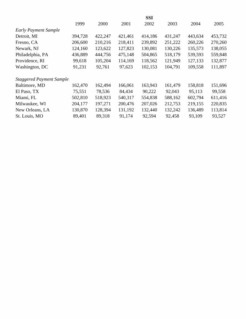
1999 2000 2001 2002 2003 2004 2005Early Payment SampleDetroit, MI 394,728 422,247 421,461 414,186 431,247 443,634 453,732Fresno, CA 206,600 210,216 218,411 239,892 251,222 260,226 270,260Newark, NJ 124,160 123,622 127,823 130,081 130,226 135,573 138,055Philadelphia, PA 436,889 444,756 475,148 504,865 518,179 539,593 559,848Providence, RI 99,618 105,204 114,169 118,562 121,949 127,133 132,877Washington, DC 91,231 92,761 97,623 102,153 104,791 109,558 111,897
Staggered Payment SampleBaltimore, MD 162,470 162,494 166,061 163,943 161,479 158,818 151,696El Paso, TX 75,551 78,536 84,434 90,222 92,043 95,113 99,558Miami, FL 502,810 518,923 540,317 554,838 588,162 602,794 611,416Milwaukee, WI 204,177 197,271 200,476 207,026 212,753 219,155 220,835New Orleans, LA 130,870 128,394 131,192 132,440 132,242 136,489 113,814St. Louis, MO 89,401 89,318 91,174 92,594 92,458 93,109 93,527
SSI