Welcome to the CLU-IN Internet Seminar

Unified Statistical GuidanceSponsored by: U.S. EPA Technology Innovation and Field Services DivisionDelivered: February 28, 2011, 2:00 PM - 4:00 PM, EST (19:00-21:00 GMT)

Instructors:Kirk Cameron, MacStat Consulting, Ltd (kcmacstat@qwest.net)

Mike Gansecki, U.S. EPA Region 8 (gansecki.mike@epa.gov)Moderator:

Jean Balent, U.S. EPA, Technology Innovation and Field Services Division (balent.jean@epa.gov)

Visit the Clean Up Information Network online at www.cluin.org 1

2

Housekeeping• Please mute your phone lines, Do NOT put this call on hold

– press *6 to mute #6 to unmute your lines at anytime (or applicable instructions)

• Q&A • Turn off any pop-up blockers• Move through slides using # links on left or buttons

• This event is being recorded • Archives accessed for free http://cluin.org/live/archive/

Go to slide 1

Move back 1 slide

Download slides as PPT or PDF

Move forward 1 slide

Go to seminar

homepage

Submit comment or question

Report technical problems

Go to last slide

33

UNIFIED GUIDANCE UNIFIED GUIDANCE WEBINARWEBINAR

Statistical Analysis of Groundwater Statistical Analysis of Groundwater Monitoring Data at RCRA FacilitiesMonitoring Data at RCRA Facilities

March 2009March 2009

Website Location: Website Location: http://www.epa.gov/epawaste/hazard/correctiveahttp://www.epa.gov/epawaste/hazard/correctiveaction/resources/guidance/sitechar/gwstats/ction/resources/guidance/sitechar/gwstats/index.htmindex.htm

44

Covers and

Errata Sheet

2010

55

Purpose of WebinarPurpose of Webinar

• Present general layout and contents of the Present general layout and contents of the Unified GuidanceUnified Guidance

• How to use this guidanceHow to use this guidance

• Issues of interestIssues of interest

• Specific Guidance Details Specific Guidance Details

66

GENERAL LAYOUTGENERAL LAYOUT

Longleat, England

77

GUIDANCE LAYOUTGUIDANCE LAYOUT

MAIN TEXTMAIN TEXTPART I Introductory Information & DesignPART I Introductory Information & Design

PART II Diagnostic MethodsPART II Diagnostic Methods

PART III Detection Monitoring MethodsPART III Detection Monitoring Methods

PART IV Compliance/Corrective Action MethodsPART IV Compliance/Corrective Action Methods

APPENDICES– References, Index, APPENDICES– References, Index, Historical Issues, Statistical Details, Historical Issues, Statistical Details, Programs & TablesPrograms & Tables

88

PART I INTRODUCTORY PART I INTRODUCTORY INFORMATION & DESIGNINFORMATION & DESIGN

• Chapter 2 RCRA Regulatory OverviewChapter 2 RCRA Regulatory Overview

• Chapter 3 Key Statistical ConceptsChapter 3 Key Statistical Concepts

• Chapter 4 Groundwater Monitoring Chapter 4 Groundwater Monitoring FrameworkFramework

• Chapter 5 Developing Background DataChapter 5 Developing Background Data

• Chapter 6 Detection Monitoring DesignChapter 6 Detection Monitoring Design

• Chapter 7 Compliance/Corrective Action Chapter 7 Compliance/Corrective Action Monitoring DesignMonitoring Design

• Chapter 8 Summary of MethodsChapter 8 Summary of Methods

99

PART II DIAGNOSTIC PART II DIAGNOSTIC METHODSMETHODS• Chapter 9 Exploratory Data TechniquesChapter 9 Exploratory Data Techniques

• Chapter 10 Fitting DistributionsChapter 10 Fitting Distributions

• Chapter 11 Outlier AnalysesChapter 11 Outlier Analyses

• Chapter 12 Equality of Variance Chapter 12 Equality of Variance

• Chapter 13 Spatial Variation EvaluationChapter 13 Spatial Variation Evaluation

• Chapter 14 Temporal Variation AnalysisChapter 14 Temporal Variation Analysis

• Chapter 15 Managing Non-Detect DataChapter 15 Managing Non-Detect Data

1010

PART III DETECTION PART III DETECTION MONITORING METHODSMONITORING METHODS

• Chapter 16 Two-sample TestsChapter 16 Two-sample Tests

• Chapter 17 ANOVAs, Tolerance Chapter 17 ANOVAs, Tolerance Limits & Trend TestsLimits & Trend Tests

• Chapters 18 Prediction Limit PrimerChapters 18 Prediction Limit Primer

• Chapter 19 Prediction Limit Chapter 19 Prediction Limit Strategies With RetestingStrategies With Retesting

• Chapter 20 Control ChartsChapter 20 Control Charts

1111

PART IV COMPLIANCE PART IV COMPLIANCE MONITORING METHODSMONITORING METHODS• Chapter 21 Confidence Interval TestsChapter 21 Confidence Interval Tests• Mean, Median and Upper Percentile Tests Mean, Median and Upper Percentile Tests

with Fixed Health-based Standardswith Fixed Health-based Standards• Stationary versus Trend TestsStationary versus Trend Tests• Parametric and Non-parametric OptionsParametric and Non-parametric Options• Chapter 22 Strategies under Compliance Chapter 22 Strategies under Compliance

and Corrective Action Testingand Corrective Action Testing• Section 7.5 Consideration of Tests with a Section 7.5 Consideration of Tests with a

Background-type Groundwater Protection Background-type Groundwater Protection StandardStandard

1212

HOW TO USE THIS HOW TO USE THIS GUIDANCEGUIDANCE

Man-at-Desk

1313

USING THE UNIFIED USING THE UNIFIED GUIDANCEGUIDANCE• Design Design of a statistical monitoring system of a statistical monitoring system

versusversus routine implementationroutine implementation• FlexibilityFlexibility necessary in selecting methods necessary in selecting methods• Resolving issuesResolving issues may require coordination may require coordination

with the regulatory agencywith the regulatory agency• Later detailed methods based on early Later detailed methods based on early

concept and concept and design Chaptersdesign Chapters• Each methodEach method has background, has background,

requirements and assumptions, procedure requirements and assumptions, procedure and a worked exampleand a worked example

1414

The NeumannsThe Neumanns

Alfred E. Neuman, Cover of MAD #30 John von Neumann, taken in the 1940’s

1515

Temporal Variation [Chapter Temporal Variation [Chapter 14]14]Rank von Neumann Ratio Test Rank von Neumann Ratio Test Background & PurposeBackground & Purpose• A non-parametric test of first-order autocorrelation; A non-parametric test of first-order autocorrelation;

an alternative to the autocorrelation functionan alternative to the autocorrelation function

• Based on idea that independent data vary in a random but Based on idea that independent data vary in a random but predictable fashionpredictable fashion

• Ranks of sequential lag-1 pairs are tested, using the sum of Ranks of sequential lag-1 pairs are tested, using the sum of squared differences in a ratiosquared differences in a ratio

• Low values of the ratio v indicative of temporal dependenceLow values of the ratio v indicative of temporal dependence

• A powerful non-parametric test even with parametric (normal or A powerful non-parametric test even with parametric (normal or skewed) data skewed) data

1616

Temporal Variation [Chapter Temporal Variation [Chapter 14]14]Rank von Neumann Ratio TestRank von Neumann Ratio TestRequirement & AssumptionsRequirement & Assumptions• An unresolved problem occurs when a substantial fraction An unresolved problem occurs when a substantial fraction

of tied observations occursof tied observations occurs

• Mid-ranks are used for ties, but no explicit adjustment has Mid-ranks are used for ties, but no explicit adjustment has been developedbeen developed

• Test may not be appropriate with a large fraction of non-Test may not be appropriate with a large fraction of non-detect data; most non-parametric tests may not work welldetect data; most non-parametric tests may not work well

• Many other non-parametric tests are also available in the Many other non-parametric tests are also available in the statistical literature, particularly with normally distributed statistical literature, particularly with normally distributed residuals following trend removalresiduals following trend removal

1717

Temporal Variation [Chapter Temporal Variation [Chapter 14]14]Rank von Neumann Ratio Rank von Neumann Ratio ProcedureProcedure

1818

Rank von Neumann Example Rank von Neumann Example 14-414-4

Arsenic DataArsenic Data

1919

Rank von Neumann Ex.14-4 Rank von Neumann Ex.14-4 SolutionSolution

2020

DIAGNOSTIC TESTING DIAGNOSTIC TESTING Preliminary Data Plots [Chapter 9]Preliminary Data Plots [Chapter 9]

2121

Additional Diagnostic Additional Diagnostic InformationInformation• Data PlotsData Plots [Chapter 9] – [Chapter 9] – Indicate no likely outliers; data Indicate no likely outliers; data

are roughly normal, symmetric and stationary with no are roughly normal, symmetric and stationary with no obvious unequal variance across time (to be tested)obvious unequal variance across time (to be tested)

• Correlation Coefficient Normality Test Correlation Coefficient Normality Test [Section 10.6][Section 10.6]r = .99; p[r] > .1 r = .99; p[r] > .1 Accept NormalityAccept Normality

• Equality of Variance Equality of Variance [Chapter 11] - [Chapter 11] - see analyses belowsee analyses below

• Outlier Tests Outlier Tests [Chapter 12]- [Chapter 12]- not necessarynot necessary

• Spatial Variation Spatial Variation [Chapter 13]–[Chapter 13]–spatial variation not spatial variation not relevant for single variable data setsrelevant for single variable data sets

2222

Additional Diagnostic Additional Diagnostic InformationInformation• Von Neumann Ratio Test Von Neumann Ratio Test [Section 14.2.4][Section 14.2.4]

ν = 1.67 ν = 1.67 No first-order autocorrelationNo first-order autocorrelation

• Pearson Correlation of Arsenic vs. TimePearson Correlation of Arsenic vs. Time[p.3-12][p.3-12]; ; r = .09 r = .09 No apparent linear trendNo apparent linear trend

• One-Way ANOVA Test for Quarterly Differences One-Way ANOVA Test for Quarterly Differences [Section 14.2.2];F = 1.7, p(F) = .22[Section 14.2.2];F = 1.7, p(F) = .22Secondary ANOVA test for equal variance F = .41; p(F) Secondary ANOVA test for equal variance F = .41; p(F) =.748=.748No significant quarterly mean differences and equal No significant quarterly mean differences and equal variance across quartersvariance across quarters

2323

Additional Diagnostic Additional Diagnostic InformationInformation• One-Way ANOVA Test for Annual Differences One-Way ANOVA Test for Annual Differences [Chapter 14];[Chapter 14];

F = 1.96; p(F) = .175F = 1.96; p(F) = .175Secondary ANOVA test for equal variance F = 1.11; p(F) =.385Secondary ANOVA test for equal variance F = 1.11; p(F) =.385

No significant annual mean differences and equal variance No significant annual mean differences and equal variance across yearsacross years

• Non-Detect DataNon-Detect Data [Chapter 15]– [Chapter 15]– all quantitative data; evaluation all quantitative data; evaluation not needednot needed

ConclusionsConclusions

• Arsenic data are satisfactorily independent temporally, Arsenic data are satisfactorily independent temporally, random, normally distributed, stationary and of equal random, normally distributed, stationary and of equal variancevariance

2424

ISSUESISSUES

The Thinker, Musee Rodin in Paris

2525

ISSUES OF INTERESTISSUES OF INTEREST• RCRA Regulatory Statistical IssuesRCRA Regulatory Statistical Issues

• Choices of Parametric and Non-Parametric Choices of Parametric and Non-Parametric DistributionsDistributions

• Use of Other Statistical Methods and Use of Other Statistical Methods and Software, e.g., ProUCL®Software, e.g., ProUCL®

2626

RCRA Regulatory Statistical IssuesRCRA Regulatory Statistical Issues

• Four-successive sample requirements Four-successive sample requirements and independent Sampling Dataand independent Sampling Data

• Interim Status Indicator Testing Interim Status Indicator Testing RequirementsRequirements

• 1 & 5% Regulatory Testing 1 & 5% Regulatory Testing RequirementsRequirements

• Use of ANOVA and Tolerance IntervalsUse of ANOVA and Tolerance Intervals

• April 2006 Regulatory ModificationsApril 2006 Regulatory Modifications

2727

Choices of Parametric and Non-Choices of Parametric and Non-Parametric DistributionsParametric Distributions

• Under detection monitoring development, Under detection monitoring development, distribution choices are primarily determined distribution choices are primarily determined by data patternsby data patterns

• Different choices can result in a single systemDifferent choices can result in a single system

• In compliance and corrective action In compliance and corrective action monitoring, the regulatory agency may monitoring, the regulatory agency may determine which parametric distribution is determine which parametric distribution is appropriate in light of how a GWPS should be appropriate in light of how a GWPS should be interpretedinterpreted

2828

Use of Other Statistical Methods and Use of Other Statistical Methods and Software, e.g., ProUCL®Software, e.g., ProUCL®

• The Unified Guidance provides a The Unified Guidance provides a reasonable suite of methods, but by no reasonable suite of methods, but by no means exhaustivemeans exhaustive

• Statistical literature references to other Statistical literature references to other possible tests are providedpossible tests are provided

• The guidance suggests use of R-script and The guidance suggests use of R-script and ProUCL for certain applications. Many ProUCL for certain applications. Many other commercial and proprietary software other commercial and proprietary software may be available.may be available.

2929

Lewis Hine photo, Power House Mechanic

Unified Guidance WebinarFebruary 28, 2011

Kirk Cameron, Ph.D.MacStat Consulting, Ltd.

30

Four Key Issues

•Focus on statistical design

•Spatial variation and intrawell testing

•Developing, updating BG

•Keys to successful retesting

31

Statistical Design

32

Designed for Good

•UG promotes good statistical design principles

•Do it up front

•Refine over life of facility

33

Statistical Errors?

•RCRA regulations say to ‘balance the risks of false positives and false negatives‘ — what does this mean?

•What are false positives and false negatives?

•Example: medical tests

•Why should they be balanced?

34

Errors in Testing

•False positives (α) — Deciding contamination is present when groundwater is ‘clean’

•False negatives (β) — Failing to detect real contamination

•Often work with 1–β = statistical power

35

Truth Table

Decide Truth

Clean Dirty

CleanOK

True Negative(1–α)

False Positive (α)

DirtyFalse

Negative (β)

OK True Positive Power (1–β)

36

Balancing Risk•EPA’s key interest is statistical power

•Ability to flag real contamination

•Power inversely related to false negative rate (β) by definition

•Also linked indirectly to false positive rate (α) — as α decreases so does power

•How to maintain power while keeping false positive rate low?

37

•Unified Guidance recommends using power curves to visualize a test’s effectiveness

•Plots probability of ‘triggering the test’ vs. actual state of system

•Example: kitchen smoke detector

•Alarm sounds when fire suspected

•Chance of alarm rises to 1 as smoke gets thicker

Power Curves

38

Power of the Frying Pan

39

•Performance Criterion #1 — Adequate statistical power to detect releases

•In detection monitoring, power must satisfy ‘needle in haystack’ hypothesis

•One contaminant at one well

•Measure using EPA reference power curves

UG Performance Criteria

40

• Users pick curve based on evaluation frequency

• Annual, semi-annual, quarterly

• Key targets: 55-60% at 3 SDs, 80-85% at 4 SDs

Reference Power Curves

41

•Each facility submits site-specific power curves

•Must demonstrate equivalence to EPA reference power curve

•Modern software (including R) enables this

•Weakest link principle

•One curve for each type of test

•Least powerful test must match EPA reference power curve

Maintaining Good Power?

42

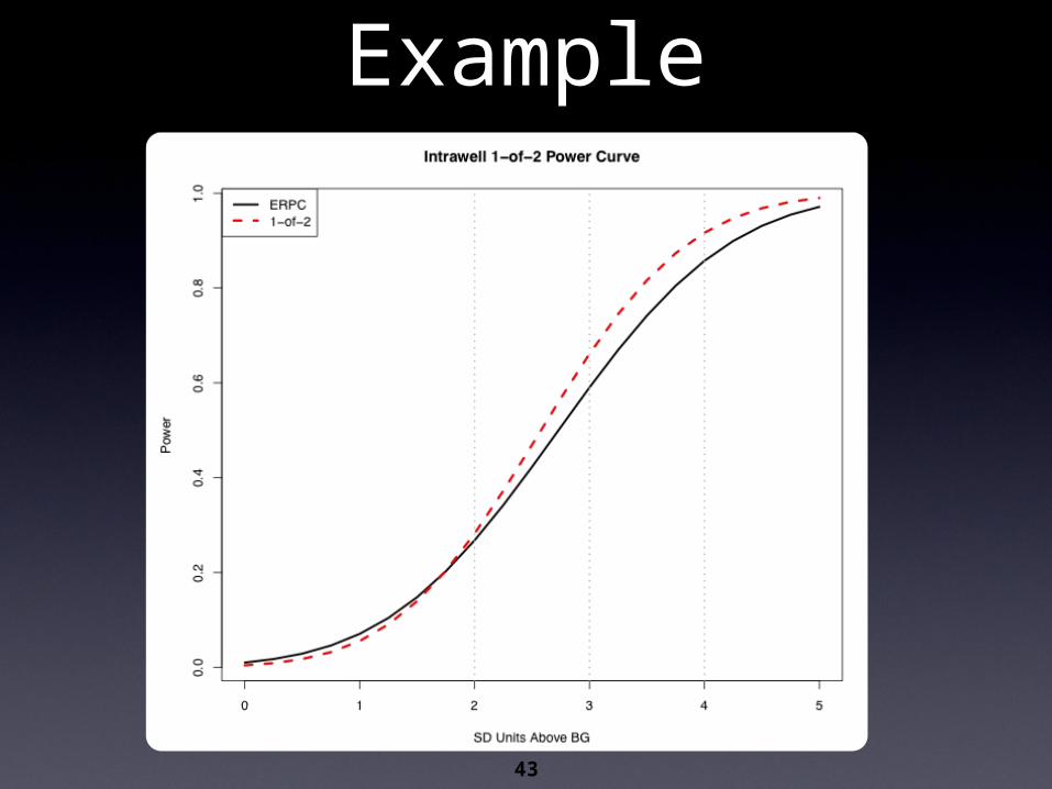
Power Curve Example

43

•Criterion #2 — Control of false positives

•Low annual, site-wide false positive rate (SWFPR) in detection monitoring

•UG recommends 10% annual target

•Same rate targeted for all facilities, network sizes

•Everyone assumes same level of risk per year

Be Not False

44

Pr 1 false + 1 .95 100 99.4%

•Chance of at least one false positive across network

•Example:100 tests, α = 5% per test

•Expect 5 or so false +’s

•Almost certain to get at least 1!

Why SWFPR?

45

SW

FP

R

Error Growth

# Simultaneous Tests46

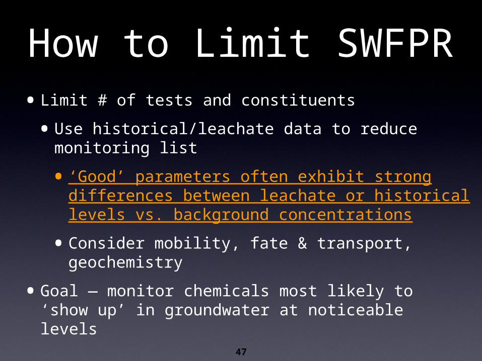
•Limit # of tests and constituents

•Use historical/leachate data to reduce monitoring list

• ‘Good’ parameters often exhibit strong differences between leachate or historical levels vs. background concentrations

•Consider mobility, fate & transport, geochemistry

•Goal — monitor chemicals most likely to ‘show up’ in groundwater at noticeable levels

How to Limit SWFPR

47

• BIG CHANGE!!

• Analytes never detected in BG not subject to formal statistics

• These chemicals removed from SWFPR calculation

• Informal test— Two consecutive detections = violation

• Makes remaining tests more powerful!

α

Double Quantification Rule

48

Final Puzzle Piece

•Use retesting with each formal test

•Improves both power and accuracy!

•Requires additional, targeted data

•Must be part of overall statistical design

49

Spatial Variation, Intrawell Testing

50

•Upgradient-downgradient

•Unless ‘leaking’/contaminated, BG and compliance samples should have same statistical distribution

•Only way to perform valid testing!

•Background and compliance wells screened in same aquifer or hydrostratigraphic unit

Traditional Assumptions

51

• Spatial Variation

• Mean concentration levels vary by location

• Average levels not constant across site

Lost in Space

52

•Spatial variation can be natural or synthetic

•Natural variability due to geochemical factors, soil deposition patterns, etc.

•Synthetic variation due to off-site migration, historical contamination, recent releases…

•Spatial variability may signal already existing contamination!

Natural vs. Synthetic

53

• Statistical test answers wrong question!

• Can’t compare apples-to-apples

• Example— upgradient-downgradient test

• Suppose sodium values naturally 20 ppm (4 SDs) higher than background on average?

• 80%+ power essentially meaningless!

Impact of Spatial Variation

54

Coastal Landfill

55

•Consider switch to intrawell tests

•UG recommends use of intrawell BG and intrawell testing whenever appropriate

•Intrawell testing approach

•BG collected from past/early observations at each compliance well

•Intrawell BG tested vs. recent data from same well

Fixing Spatial Variation

56

•Spatial variation eliminated!

•Changes measured relative to intrawell BG

•Trends can be monitored over time

•Trend tests are a kind of intrawell procedure

Intrawell Benefits

57

•Be careful of synthetic spatial differences

•Facility-impacted wells

•Hard to statistically ‘tag’ already contaminated wells

•Intrawell BG should be uncontaminated

Intrawell Cautions

58

Developing, Updating

Background

59

•Levels should be stable (stationary) over time

•Look for violations

•Distribution of BG concentrations changing

•Trend, shift, or cyclical pattern evident

BG Assumptions

60

Violations (cont.)

Seasonal Trend Concentration Shift61

•‘Stepwise’ shift in BG average

•Update BG using a ‘moving window’; discard earlier data

•Current, realistic BG levels

•Must document shifts visually and via testing

How To Fix?

62

Moving Window Approach

63

•Watch out for trends!

•If hydrogeology changes, BG should be selected to match latest conditions

•Again, might have to discard earlier BG

•Otherwise, variance too big

•Leads to loss of statistical power

Fixing (cont.)

64

•Need ≥8-10 stable BG observations

•Intrawell dilemma

•May have only 4-6 older, uncontaminated values per compliance well

•Small sample sizes especially problematic for non-parametric tests

•Solution: periodically – but carefully – update BG data pool

Small Sample Sizes

65

Updating Basics•If no contamination is flagged

•Every 2-3 years, check time series plot, run trend test

•If no trend, compare newer data to current BG

•Combine if comparable; recompute statistical limits (prediction, control)

66

Testing Compliance Standards

67

That Dang Background!

•What if natural levels higher than GWPS?

•No practical way to clean-up below BG levels!

•UG recommends constructing alternate standard

•Upper tolerance limit on background with 95% confidence, 95% tolerance

•Approximates upper 95th percentile of BG distribution

68

Retesting

69

Retesting Philosophy

•Test individual wells in new way

•Perform multiple (repeated) tests on any well suspected of contamination

•Resamples collected after initial ‘hit’

•Additional sampling & testing required, but

•Testing becomes well-constituent specific

70

•All measurements compared to BG must be statistically independent

•Each value should offer distinct, independent evidence/information about groundwater quality

•Replicates are not independent! Tend to be highly correlated — analogy to resamples

•Must ‘lag’ sampling events by allowing time between

•This includes resamples!

Important Caveat

71

•Hypothetical example

•If initial sample is an exceedance... and so is replicate or resample collected the same day/week

•What is proven or verified?

•Independent sampling aims to show persistent change in groundwater

•UG not concerned with ‘slugs’ or temporary spikes

Impact of Dependence

72

Retesting Tradeoff•Statistical benefits

•More resampling always better than less

•More powerful parametric limits

•More accurate non-parametric limits

•Practical constraints

•All resamples must be collected prior to the next regular sampling event

•How many are feasible?73

Parametric Examples

74

•(1) What if a confirmed exceedance occurs between updates?

•Detection monitoring over for that well!

•No need to update BG

•(2) Should disconfirmed, initial ‘hits’ be included when updating BG? Yes!

•Because resamples disconfirm, initial ‘hits’ are presumed to reflect previously unsampled variation within BG

Updating BG When Retesting

75

•1st 8 events = BG

•Next 5 events = tests in detection monitoring

•One initial prediction limit exceedance

Updating With Retesting

76

Summary

•Wealth of new guidance in UG

•Statistically sound, but also practical

•Good bedside reading!

77

78

Resources & Feedback

• To view a complete list of resources for this seminar, please visit the Additional Resources

• Please complete the Feedback Form to help ensure events like this are offered in the future

Need confirmation of your participation today?

Fill out the feedback form and check box for confirmation email.