welcome to day 12 principles of microeconomics. what do we want the economy to do? 1) produce a lot...
TRANSCRIPT

Welcome to Day 12
Principles of Microeconomics
What do we want the economy to do?
1) Produce a lot of stuff2)Produce the stuff we want the
most3)Distribute various things to
people who value those things highly
An economy that does these things is operating efficiently.
Efficient
The allocation of resources when the net benefits of all economic
activities are maximized.
An economy that is operating efficiently has both:
1) Efficient production2) Efficient allocation of goods.
Will a market economy do these things?
How does a business make money?Producing a lot of what people
want the most and selling it.
The better a business correctly estimates what its customers
value, and makes a lot of those things, the higher its profit.
And of course, we want the economy to be able to adjust to changing circumstances. Will a
market economy do that?
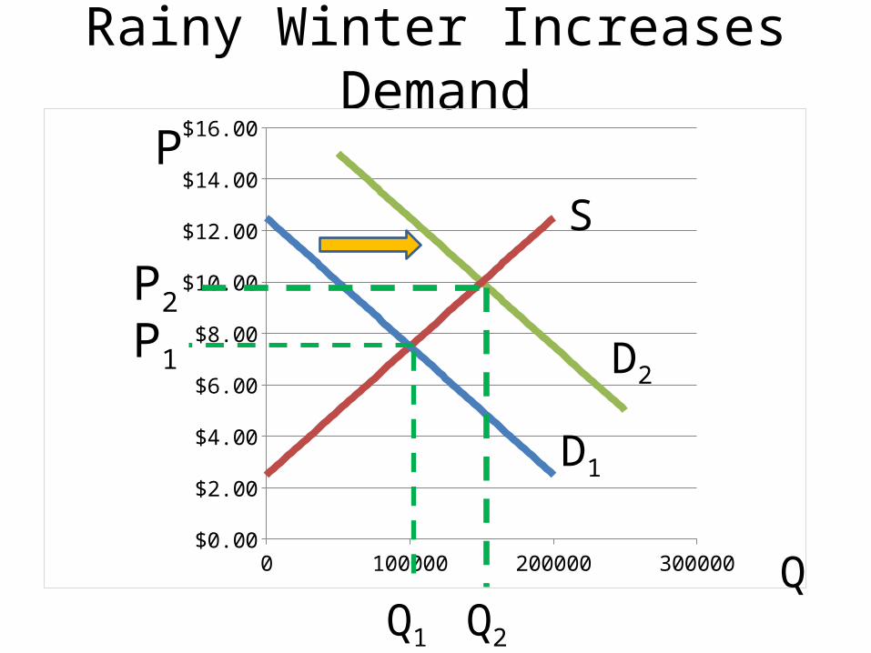
Rainy Winter Increases Demand
0 50000 100000 150000 200000 250000 300000$0.00
$2.00
$4.00
$6.00
$8.00
$10.00
$12.00
$14.00
$16.00
D1
S
P
Q
P1 D2
P2
Q1 Q2

Can a command economy do this?
The incentive problem and the information problem.

The Incentive Problem
What does an umbrella businessman get if he gets umbrellas quickly out
to a rainy area?
What does the 2nd undersecretary of umbrellas in Washington get if he
gets umbrellas quickly out to a rainy area?
The Information Problem
How does the 2nd Undersecretary of Umbrellas know we need more
umbrellas in Bakersfield?
How do private business owners of umbrella companies know?

Every time you go shopping, it is a transfer of information fest!!!

You are letting sellers know what you want.
Sellers are letting you know what they can make at what
cost.

The Invisible Hand
Adam Smith – 1776The Wealth of Nations
Because trades are voluntary, in helping yourself, when you are
helping yourself, you help others also.

The way for the businessman to make money is to most effectively
serve his customers.
In doing what is best for him, he is being lead, as if by an “invisible
hand” to help society.
So what can go wrong?
Market Failure - The failure of private decisions in the
marketplace to achieve an efficient allocation of scarce resources.

In other words, we are making too much or too little of something
because of a failure to properly take account of its benefits and costs.
What markets does the government heavily regulate in the U.S.
economy?
Externalities – an action taken by a person or firm that imposes
benefits or costs outside of any market exchange.

We’ve seen these pictures earlier this semester, but we didn’t have a name for what they were yet. Now
we do.

Welcome to Day 13
Principles of Microeconomics


So what to do?
We have seen one solution, which is government regulation of the industry.
There is another, which is to charge, or tax, people for the harm they are doing
to others. This will “internalize the externality.
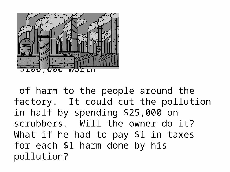
Here is our factory causing $100,000 worth of harm to the people around the factory. It could cut the pollution in half by spending $25,000 on scrubbers. Will the owner do it?What if he had to pay $1 in taxes for each $1 harm done by his pollution?

Some people have proposed a “carbon tax” as part of the solution
to global warming.

Welcome to Day 14
Principles of Microeconomics


Besides externalities, there is another type of marked failure is
known as public goods.
Public Goods
A good for which the cost of exclusion is prohibitive and for which the marginal cost of an
additional user is zero.

For example, a streetlight placed on a block.
Examples of Public Goods1) Streetlights
2) Roads3) National Defense
4) Light Houses5) Free Television
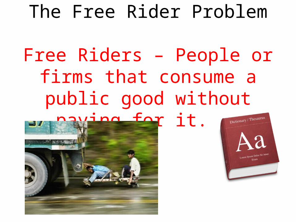
The Free Rider Problem
Free Riders – People or firms that consume a public good without
paying for it.

The government gets around the problem by not asking you to pay,
but telling you to pay.
In theory, the government can handle this problem. In practice, we still have our old problems of:
1) information.2) incentive.

Tragedy of the Commons - What happens when property rights are
not assigned?

Once property rights are assigned, problem solved. This is why the cow population is thriving and whales are hunted almost to
extinction.

The air is a commons.
Unless the government enforces regulation or taxes.
Of course, we have talked about air pollution before, under
externalities.
The tragedy of the commons isn’t really a new thing, it is a subset of
externalities.
Who owns the air?

Chapter 7The Analysis of
Consumer Choice
1. THE CONCEPT OF UTILITY
Learning Objectives1. Define what economists mean by utility.2. Distinguish between the concepts of total utility
and marginal utility.3. State the law of diminishing marginal utility and
illustrate it graphically.4. State, explain, and illustrate algebraically the
utility-maximizing condition.
1.1 Total Utility
• Total utility is the number of units of utility that a consumer gains from consuming a given quantity of a good, service, or activity during a particular time period.
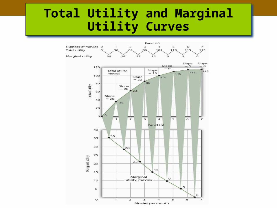
Total Utility and Marginal Utility Curves

1.2 Marginal Utility
• Marginal utility is the amount by which total utility rises with consumption of an additional unit of a good, service, or activity, all other things unchanged.
• The law of diminishing marginal utility is the tendency of marginal utility to decline beyond some level of consumption during a period.

Welcome to Day 15
Principles of Microeconomics


Write your name, class day and time, and Quiz #5 at the top of the
paper.

The Invisible Hand can work because price allows for the
effective use of 1) ____ and 2) ____ in a
market economy. Hint: both answers start with the letter
“i”.
We’ve seen that when the thing is free, the best thing to do is
just take it until marginal utility hits zero.
But what if you have to pay a price?

Now the amount of things you can take is limited, so the
question is “is getting one more of this worth giving up some of
that?”
How do you decide what to buy at the store? From an economist’s point of view, it is all about comparing how
much you like the thing to its price.
Buy the things you really like compared to their prices, and don’t buy what you don’t like very much
compared to its price.
How much you like the thing is measured by its marginal utility.
So the mathematical way to write out the comparison of how much you like one more
unit of X compared to the price of X is MUX
PX
MUX
PX
Can also be understood as the utils you get in return for spending $1 more
on the good.
Spend your dollars on whatever gets you the higher return on those dollars.
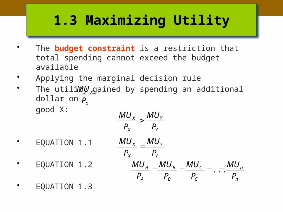
1.3 Maximizing Utility
• The budget constraint is a restriction that total spending cannot exceed the budget available
• Applying the marginal decision rule• The utility gained by spending an additional dollar on
good X:
• EQUATION 1.1
• EQUATION 1.2
• EQUATION 1.3
X
X
P
MU
Y
Y
X
X
P
MU
P
MU
Y
Y
X
X
P
MU
P
MU
n
n
C
C
B
B
A
A
P
MU
P
MU
P
MU
P
MU ...

• Equation 1.3 states:– Utility maximizing condition: Utility is
maximized when total outlays equal the budget available and when the ratios of marginal utilities to prices are equal for all goods and services.
• The problem of divisibility:– The marginal decision rule to utility maximization can be
applied only when the goods are divisible
1.3 Maximizing Utility
2. UTILITY MAXIMIZATION AND DEMAND
Learning Objectives1. Derive an individual demand curve from utility-
maximizing adjustments to changes in price.2. Derive the market demand curve from the
demand curves of individuals.3. Explain the substitution and income effects of a
price change.4. Explain the concepts of normal and inferior
goods in terms of the income effect.

2.1 Deriving an Individual’s Demand Curve
• Example: Mary Andrews consumes only apples, denoted by A and oranges, denoted by O– Apples cost $2 per pound – Oranges cost $1 per pound– Budget allows her to spend $20 per month on the two
goods
• Equation 2.1
• Equation 2.2
• Equation 2.3
1$2$OA MUMU
1$1$OA MUMU
1$1$OA MUMU

Utility Maximization and an Individual’s Demand Curve

Deriving a Market Demand Curve
Chapter 8
Production and Cost
1. PRODUCTION CHOICES AND COSTS: THE SHORT RUN
Learning Objectives1. Understand the terms associated with the short-run production
function—total product, average product, and marginal product—and explain and illustrate how they are related to each other.
2. Explain the concepts of increasing, diminishing, and negative marginal returns and explain the law of diminishing marginal returns.
3. Understand the terms associated with costs in the short run—total variable cost, total fixed cost, total cost, average variable cost, average fixed cost, average total cost, and marginal cost—and explain and illustrate how they are related to each other.
4. Explain and illustrate how the product and cost curves are related to each other and to determine in what ranges on these curves marginal returns are increasing, diminishing, or negative.
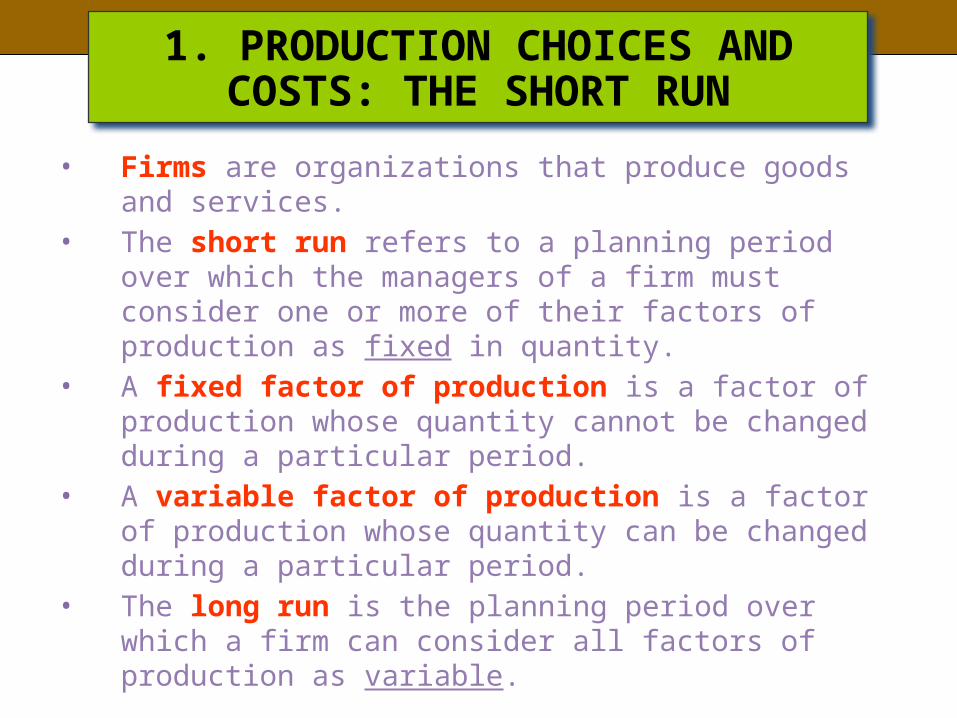
1. PRODUCTION CHOICES AND COSTS: THE SHORT RUN
• Firms are organizations that produce goods and services.
• The short run refers to a planning period over which the managers of a firm must consider one or more of their factors of production as fixed in quantity.
• A fixed factor of production is a factor of production whose quantity cannot be changed during a particular period.
• A variable factor of production is a factor of production whose quantity can be changed during a particular period.
• The long run is the planning period over which a firm can consider all factors of production as variable.

Welcome to Day 16
Principles of Microeconomics


1.1 The Short-Run Production Function
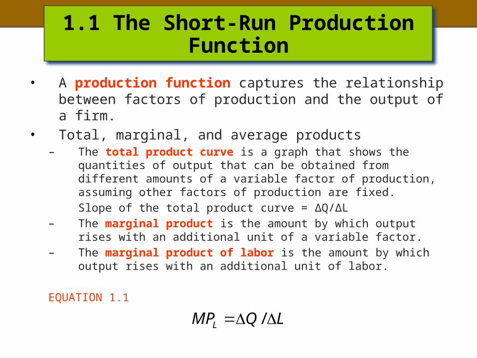
• A production function captures the relationship between factors of production and the output of a firm.
• Total, marginal, and average products– The total product curve is a graph that shows the quantities
of output that can be obtained from different amounts of a variable factor of production, assuming other factors of production are fixed.
Slope of the total product curve = ΔQ/ΔL– The marginal product is the amount by which output rises
with an additional unit of a variable factor.– The marginal product of labor is the amount by which
output rises with an additional unit of labor.
EQUATION 1.1LQMPL /
1.1 The Short-Run Production Function
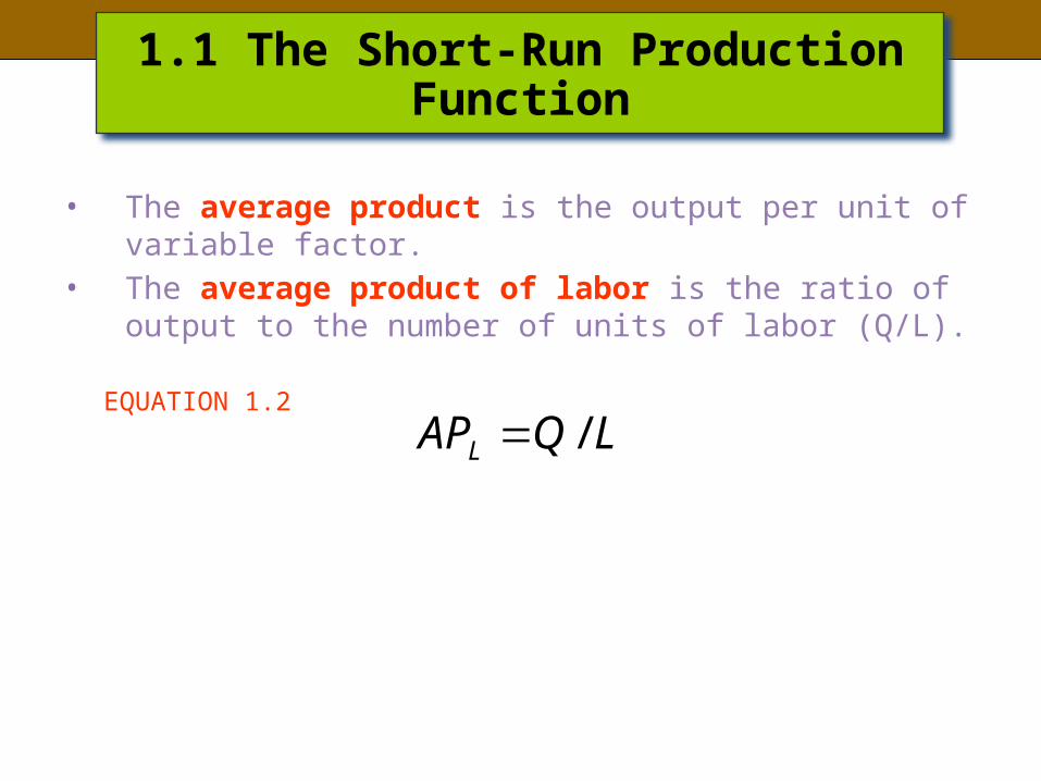
• The average product is the output per unit of variable factor.
• The average product of labor is the ratio of output to the number of units of labor (Q/L).
EQUATION 1.2LQAPL /
1.1 The Short-Run Production Function
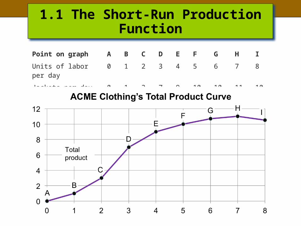
Point on graph A B C D E F G H I
Units of labor per day 0 1 2 3 4 5 6 7 8
Jackets per day 0.0 1.0 3.0 7.0 9.0 10.0 10.7 11.0 10.5
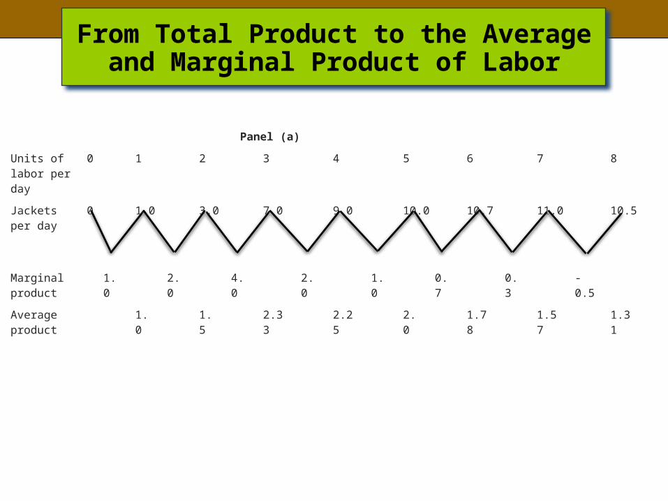
From Total Product to the Average and Marginal Product of Labor
Panel (a)
Units of labor per day
0 1 2 3 4 5 6 7 8
Jackets per day
0 1.0 3.0 7.0 9.0 10.0 10.7 11.0 10.5
Marginal product
1.0 2.0 4.0 2.0 1.0 0.7 0.3 -0.5
Average product
1.0 1.5 2.33 2.25 2.0 1.78 1.57 1.31
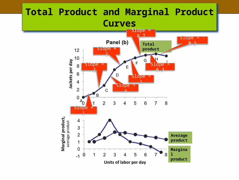
Total Product and Marginal Product Curves
Total product
Marginal product
Slope = -0.5
Slope = 0.3
Slope = 0.7
Slope = 1
Slope = 2
Slope = 4
Slope = 2
Average product
Slope = 1

Welcome to Day 17
Principles of Microeconomics


Write your name, class day and time, and Quiz #6 at the top of the
paper.

Answer whether the following statement is true, false, or uncertain,
and explain your answer.
A person at the donut shop will buy donuts until the marginal utility of the
next donut is zero or negative.
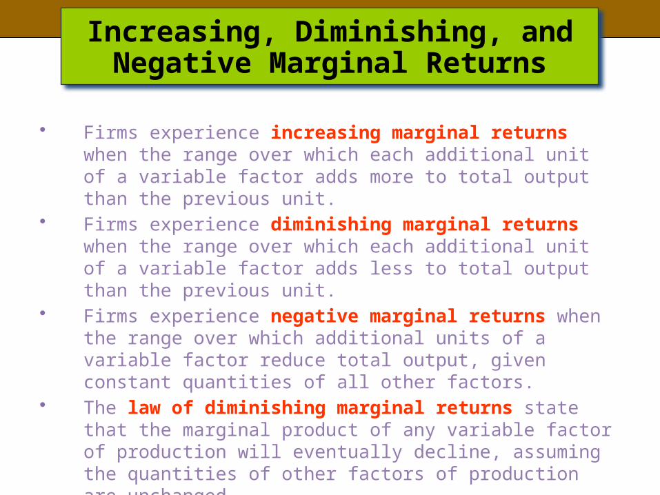
Increasing, Diminishing, and Negative Marginal Returns
• Firms experience increasing marginal returns when the range over which each additional unit of a variable factor adds more to total output than the previous unit.
• Firms experience diminishing marginal returns when the range over which each additional unit of a variable factor adds less to total output than the previous unit.
• Firms experience negative marginal returns when the range over which additional units of a variable factor reduce total output, given constant quantities of all other factors.
• The law of diminishing marginal returns state that the marginal product of any variable factor of production will eventually decline, assuming the quantities of other factors of production are unchanged.

Increasing, Diminishing, and Negative Marginal Returns
Increasing marginal returns
Neg
ativ
e m
arg
inal
ret
urns
Diminishing marginal returns
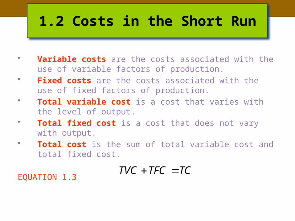
1.2 Costs in the Short Run
• Variable costs are the costs associated with the use of variable factors of production.
• Fixed costs are the costs associated with the use of fixed factors of production.
• Total variable cost is a cost that varies with the level of output.
• Total fixed cost is a cost that does not vary with output.• Total cost is the sum of total variable cost and total fixed
cost.
EQUATION 1.3 TCTFCTVC
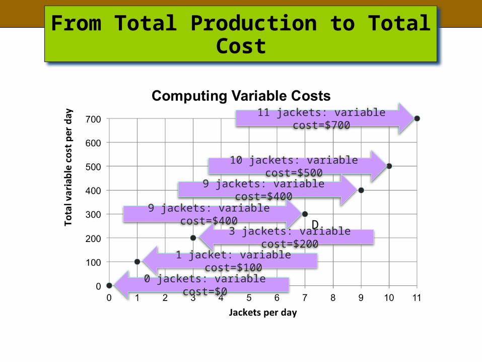
From Total Production to Total Cost
D’
11 jackets: variable cost=$700
10 jackets: variable cost=$500
9 jackets: variable cost=$400
9 jackets: variable cost=$400
3 jackets: variable cost=$200
1 jacket: variable cost=$100
0 jackets: variable cost=$0
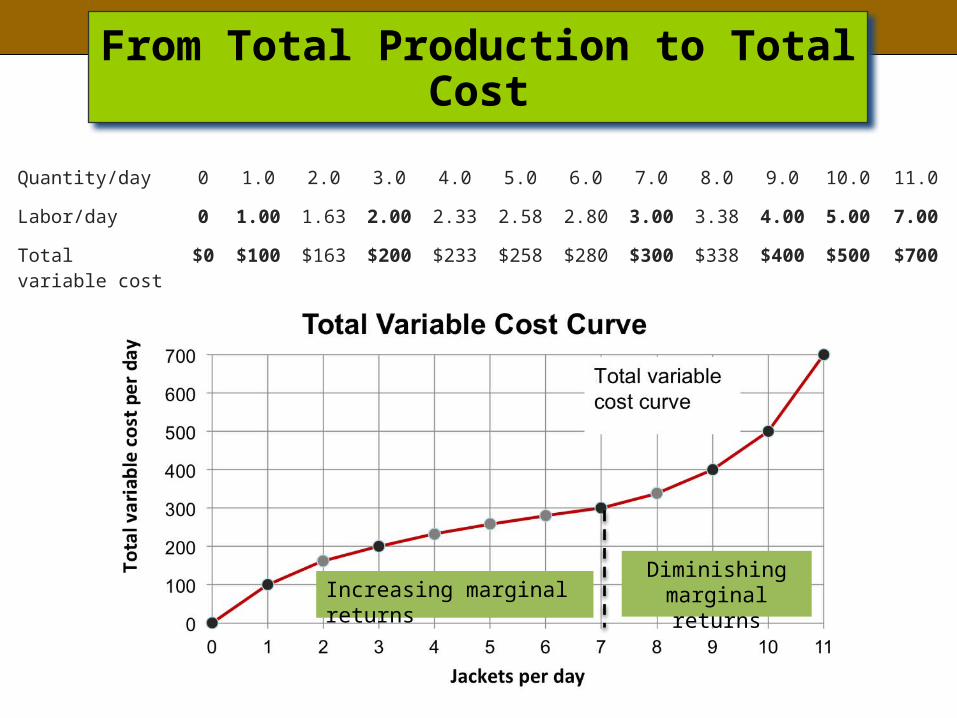
From Total Production to Total Cost
Quantity/day 0 1.0 2.0 3.0 4.0 5.0 6.0 7.0 8.0 9.0 10.0 11.0
Labor/day 0 1.00 1.63 2.00 2.33 2.58 2.80 3.00 3.38 4.00 5.00 7.00
Total variable cost $0 $100 $163 $200 $233 $258 $280 $300 $338 $400 $500 $700
Increasing marginal returnsDiminishing
marginal returns
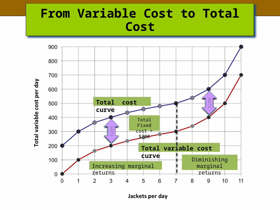
From Variable Cost to Total Cost
Increasing marginal returnsDiminishing
marginal returns
Total cost curve
Total Fixed cost = $200
$200
$200
Total variable cost curve

Marginal and Average Costs
• Average total cost is total cost divided by quantity; it is the firms total cost per unit of output.
EQUATION 1.4
• Average variable cost is total variable cost dIvided by quantity; it is the firm’s total variable cost per unit of output.
EQUATION 1.5
• Average fixed cost is total fixed cost divided by quantity.EQUATION 1.6
EQUATION 1.7
EQUATION 1.8
QTCATC /
QTVCAVC /
QTFCAFC /
QTCMC /
ATCAFCAVC
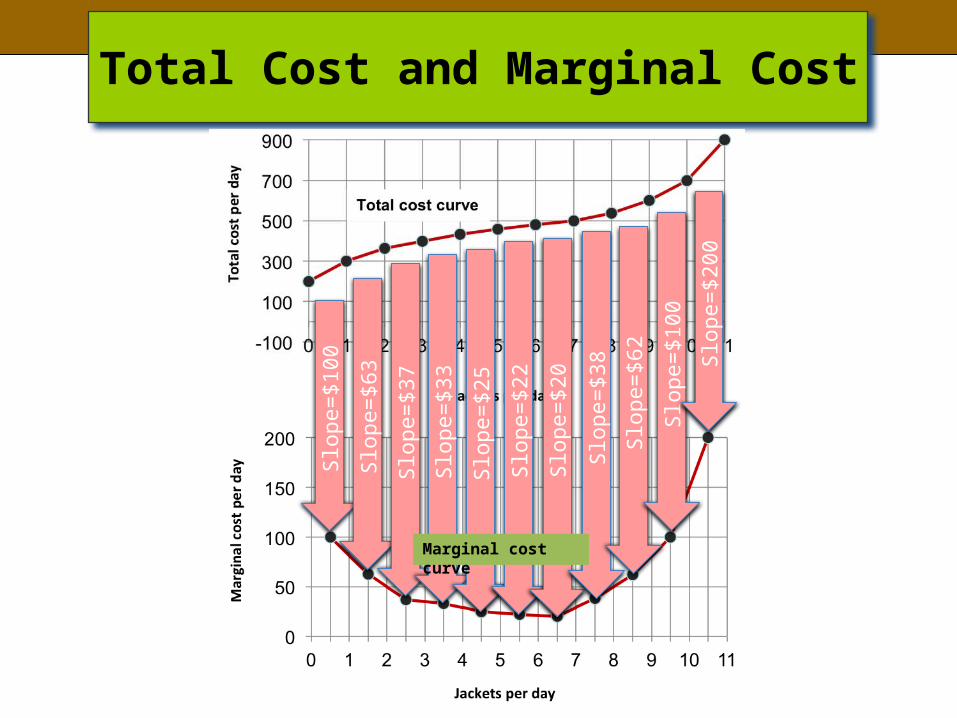
Total Cost and Marginal Cost
Slop
e=$1
00
Slop
e=$6
3
Slop
e=$3
7
Slop
e=$3
3
Slop
e=$2
5
Slop
e=$2
2
Slop
e=$2
0
Slop
e=$3
8
Slop
e=$6
2
Slop
e=$1
00
Slop
e=$2
00
Marginal cost curve
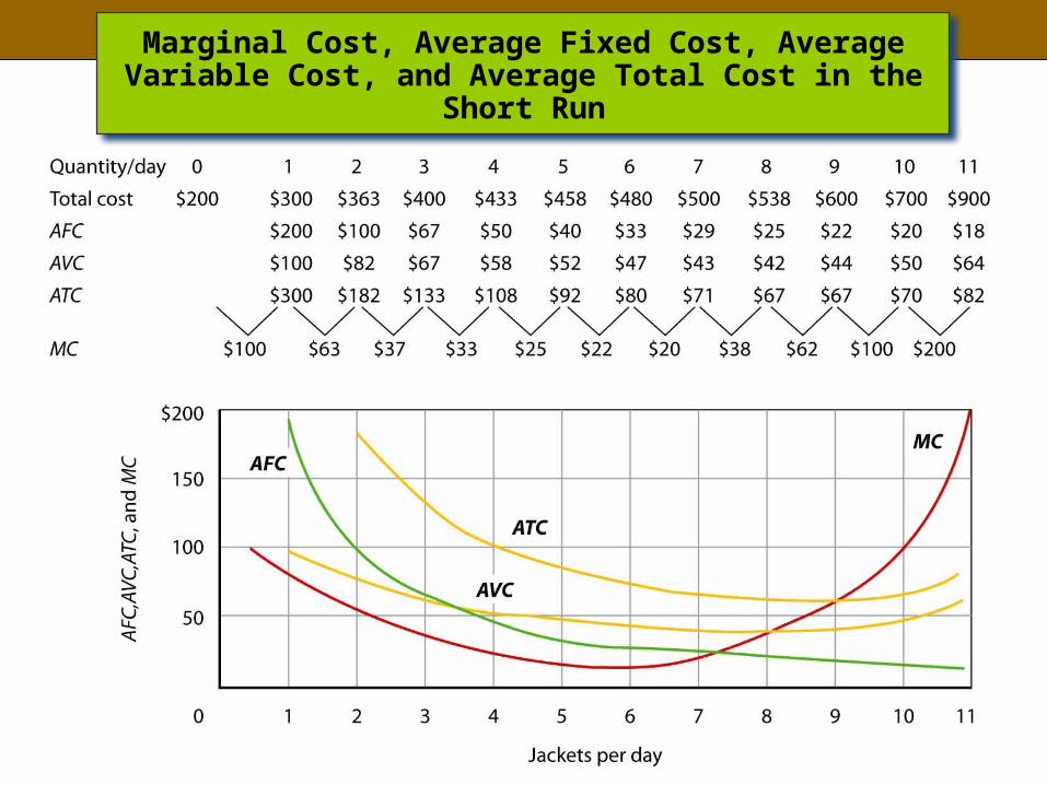
Marginal Cost, Average Fixed Cost, Average Variable Cost, and Average Total Cost in the
Short Run

Welcome to Day 18
Principles of Microeconomics


2. PRODUCTION CHOICES AND COSTS: THE LONG RUN
Learning Objectives1. Apply the marginal decision rule to explain how a firm chooses
its mix of factors of production in the long run.2. Define the long-run average cost curve and explain how it
relates to economies and diseconomies or scale.
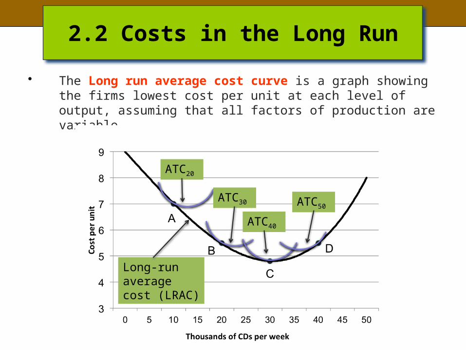
2.2 Costs in the Long Run
• The Long run average cost curve is a graph showing the firms lowest cost per unit at each level of output, assuming that all factors of production are variable.
ATC20
Long-run average cost (LRAC)
ATC30
ATC40
ATC50

Economies and Diseconomies of Scale
• Economies of scale refers to a situation in which the long run average cost declines as the firm expands its output.
• Diseconomies of scale refers to a situation in which the long run average cost increases as the firm expands its output.
• Constant returns to scale refers to a situation in which the long run average cost stays the same over an output range.
Economies of scale
Constant returns to scale
Diseconomies of scale
Economies and diseconomies of scale affect the sizes of firms operating in a
market.

Reasons for Economies of Scale1) Mass Production Assembly Line
Machines.2) Specialization of Labor.
Reasons for Diseconomies of Scale1) Command and Control Problems.
2) Law of Increasing Opportunity Cost (the additional workers are getting worse).

Welcome to Day 19
Principles of Microeconomics


Write your name, class day and time, and Quiz #7 at the top of the
paper.
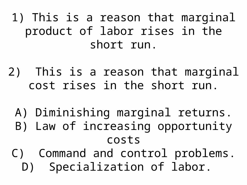
1) This is a reason that marginal product of labor rises in the short run.
2) This is a reason that marginal cost rises in the short run.
A) Diminishing marginal returns.B) Law of increasing opportunity costsC) Command and control problems.
D) Specialization of labor.
Chapter 9
Competitive Markets
for Goods and
Services
1. PERFECT COMPETITION: A MODEL
Learning Objectives1. Explain what economists mean by perfect competition.2. Identify the basic assumptions of the model of perfect
competition and explain why they imply price-taking behavior.

1. PERFECT COMPETITION: A MODEL
• Perfect competition is a model of the market based on the assumption that a large number of firms produce identical goods consumed by a large number of buyers.

1.1 Assumptions of the Model
• Price takers are individuals or firms who must take the market price as given.
– Identical goods– A large number of buyers and
sellers– Ease of entry and exit
2. OUTPUT DETERMINATION IN THE SHORT RUN
Learning Objectives1. Show graphically how an individual firm in a
perfectly competitive market can use total revenue and total cost curves or marginal revenue and marginal cost curves to determine the level of output that will maximize its economic profit.
2. Explain when a firm will shut down in the short run and when it will operate even if it is incurring economic losses.
3. Derive the firm’s supply curve from the firm’s marginal cost curve and the industry supply curve from the supply curves of individual firms.

The Market for Radishes
Total Revenue
• Total revenue is a firm’s output multiplied by the price at which it sells that output.
• EQUATION 2.1
QPTR
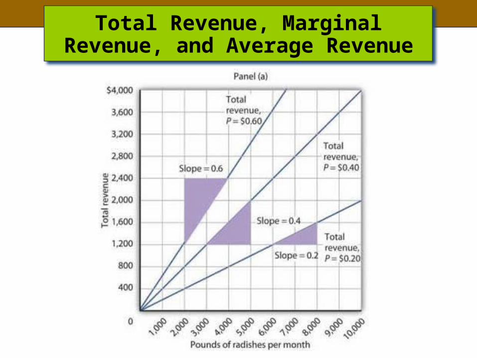
Total Revenue, Marginal Revenue, and Average Revenue
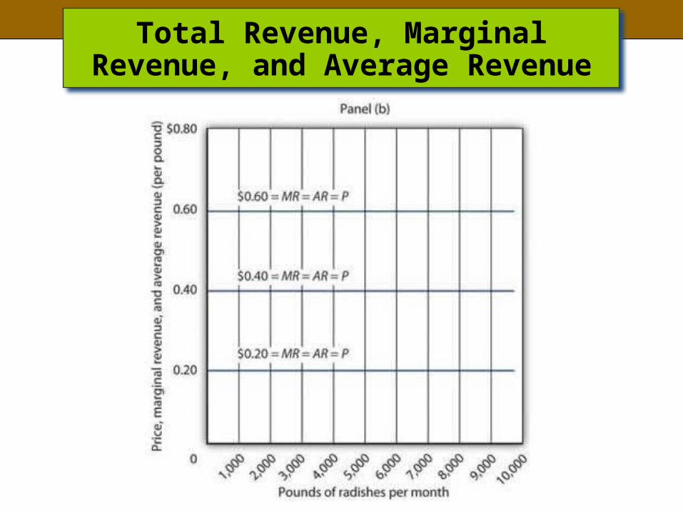
Total Revenue, Marginal Revenue, and Average Revenue
Price, Marginal Revenue, and Average Revenue
• Marginal revenue is the increase in total revenue when the quantity supplied is raised by one unit.
• For a perfectly competitive firm, the marginal revenue is equal to the price per unit of the good being sold.
• In a perfectly competitive market, marginal revenue curve is the demand curve that a firm faces.
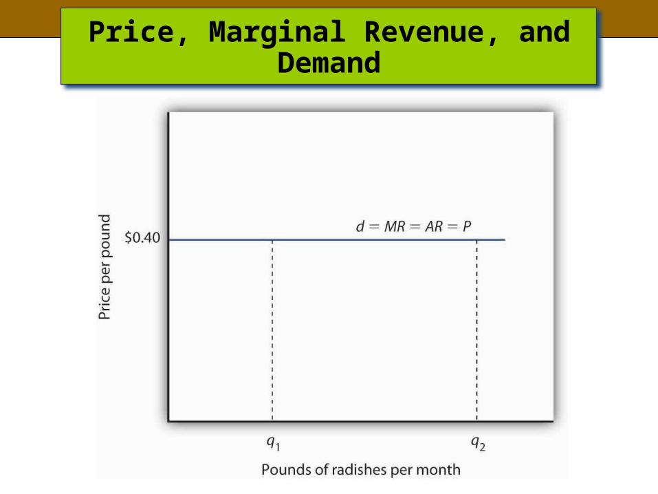
Price, Marginal Revenue, and Demand
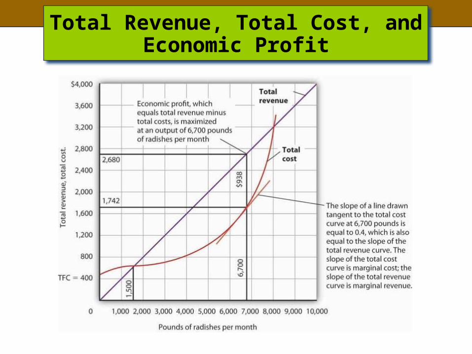
Total Revenue, Total Cost, and Economic Profit
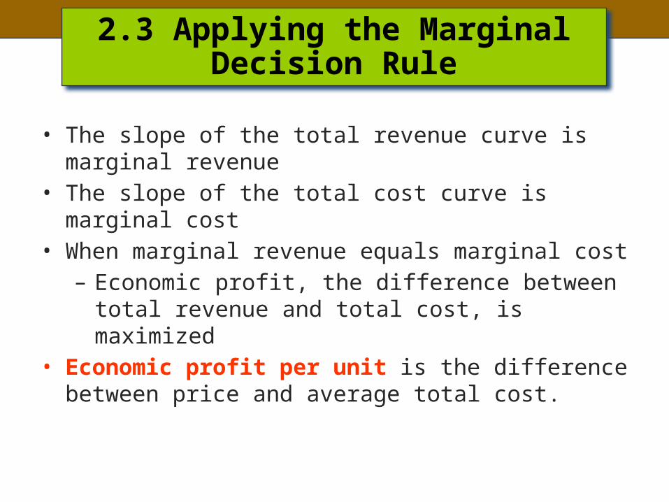
2.3 Applying the Marginal Decision Rule
• The slope of the total revenue curve is marginal revenue
• The slope of the total cost curve is marginal cost• When marginal revenue equals marginal cost
– Economic profit, the difference between total revenue and total cost, is maximized
• Economic profit per unit is the difference between price and average total cost.

Applying the Marginal Decision Rule
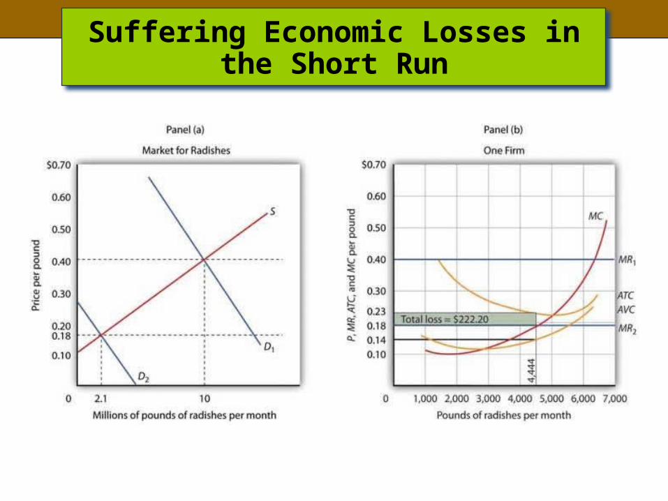
Suffering Economic Losses in the Short Run

Welcome to Day 20
Principles of Microeconomics


Write your name, class day and time, and Quiz #8 at the top of the
paper.

Write down one of the two reasons given in class for
average total costs to rise in the long run. This question is worth
1 point.
Economic Profit = Total Revenue minus Total Cost.
Total cost includes all the implicit costs of production also,
such as the value of your time and the rental/sales value of
resources you own.
•TR goes below TVC• P goes below AVC
Shutdown Point
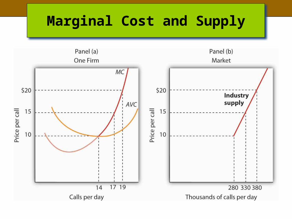
Marginal Cost and Supply
In the long-run, if there are economic profits, there will be
entry.
If there are economic losses, there will exit.
3.1 Economic Profit and Economic Loss in the Long Run
• The long run and zero economic profits - • Economic profits in a system
of perfectly competitive markets will, in the long run, be driven to zero in all industries
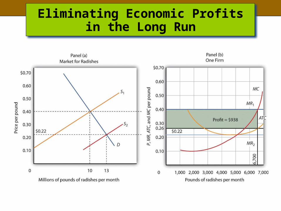
Eliminating Economic Profits in the Long Run
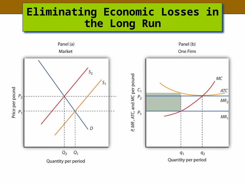
Eliminating Economic Losses in the Long Run

3.1 Economic Profit and Economic Loss
• Entry, exit, and production costs– Constant-cost industry is when expansion of the
industry does not affect the prices of factors of production
– Increasing-cost industry is an industry in which the entry of new firms bids up the prices of factors of production and thus increases production costs
– Decreasing-cost industry is an industry in which production costs fall as firms enter in the long run
– Long-run industry supply curve is a curve that relates the price of a good or service to the quantity produced after all long-run adjustments to a price change have been completed.
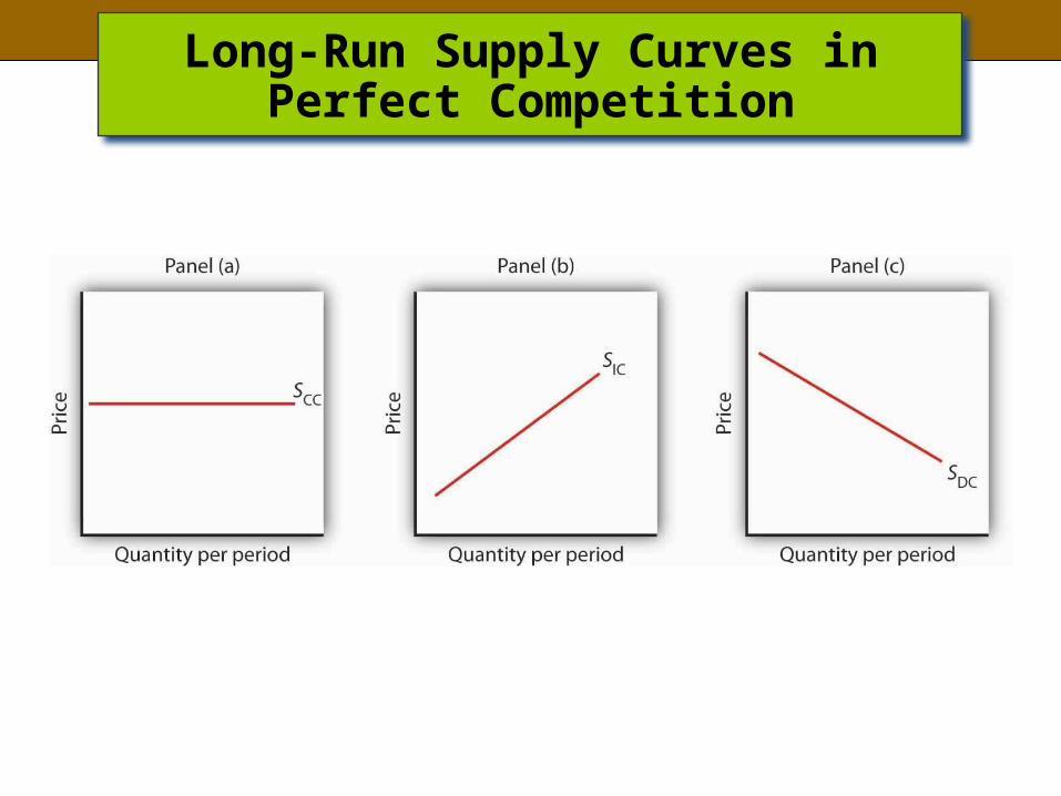
Long-Run Supply Curves in Perfect Competition
3.2 Changes in Demand
• Changes in demand occur due to a change in:• Preferences• Incomes• The price of a related good• Population• Consumer expectations
• A change in demand causes a change in the market price
– Thus shifting the marginal revenue curves of firms in the industry
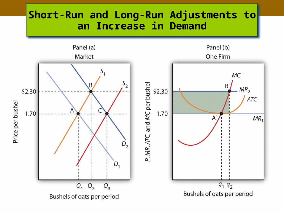
Short-Run and Long-Run Adjustments to an Increase in Demand