weighted least squares estimation for - columbia universityim2131/ps/huffmckjasa.pdf · weighted...

Weighted Least Squares Estimation for Aalen's Additive Risk Model

FRED W. HUFFER and IAN W. MCKEAGUE*

Cox's proportional hazards model has so far been the most popular model for the regression analysis of censored survival data. However, the additive risk model of Aalen can provide a useful and biologically more plausible alternative. Aalen's model

stipulates that the conditional hazard function for a subject, whose covariates are Y = (YI, ..., Ye)', has the form h(t I Y) = Y'a(t), where a = (a,, ..., ap)' is an unknown vector of hazard functions. This article discusses inference for a based on a weighted least squares (WLS) estimator of the vector of cumulative hazard functions. The asymptotic distribution of the WLS estimator is derived and used to obtain confidence intervals and bands for the cumulative hazard functions. Both a grouped data and a continuous data version of the estimator are examined. An extensive simulation study is carried out. The method is applied to grouped data on the incidence of cancer mortality among Japanese atomic bomb survivors.

KEY WORDS: Atomic bomb survivors; Grouped survival data; Martingale methods; MonteCarlo; Multivariate counting pro- cesses; Nonproportional hazards.

1. INTRODUCTION

In this article we study Aalen's (1980) additive risk model

for the regression analysis of censored survival data. Let

h(t) = h(t I Y) denote the conditional hazard function at time t for subject i whose covariates are given by the p

vector Y = (Y1, ..., YP)'. Aalen's model stipulates that p

hi(t) = a,(t)Yi, = Y'a(t) (.1 J= I

where a (a,, ..., ap)' is an unknown vector of hazard functions.

The additive risk model provides a useful alternative to

Cox's (1972) proportional hazards model. Since temporal

effects are not assumed to be proportional for each covar-

iate, Aalen's model is capable of providing detailed infor-

mation concerning the temporal influence of each covariate not available from Cox's model. In studies of excess risk

for instance, where the background risk and excess risk typ- ically can have very different temporal forms, additive risk

models seem to be biologically more plausible than pro-

portional hazard models (see Buckley 1984). For example, the latent period for the risk of cancer following exposure to low doses of ionizing radiation can be better understood

in terms of an additive risk model. Moreover, the use of the proportional hazards model when the true model is ad-

ditive risk has been found by O'Neill (1986) to result in serious asymptotic bias.

Although parametric additive risk models have been widely

* Fred W. Huffer is Associate Professor and Ian W. McKeague is Associate Professor, Department of Statistics, Florida State University, Tallahassee, FL 32306-3033. Fred W. Huffer's research was supported by the Office of Naval Research under Grant N00014-86-K-0156. Ian W. McKeague's research was supported by the Army Research Office under Grant DAAL03-86-K-0094. The authors are grateful to the associate ed- itor and a referee for their detailed comments. We also thank Richard Gill for a helpful discussion concerning the WLS estimator at the Ob- erwolfach meeting on martingale methods in statistics in December 1988, and David Hoel for telling us how to procure the data used in Section 4. These data were supplied by RERF, which is a private foundation that is funded equally by the Japanese Ministry of Health and Welfare and the U.S. Department of Energy through the U.S. National Academy of Sciences. The conclusions reached in this article are those of the authors and do not necessarily reflect the scientific judgment of RERF or its fund- ing agencies.

applied in survival analysis (especially in epidemiology) for

many years (see the references in Breslow 1986; Muirhead

and Darby 1987), the nonparametric additive risk model (1. 1) has only been studied recently (Aalen 1980, 1989; McKeague 1986, 1988a, b; Huffer and McKeague 1987;

Mau 1986, 1988).

Aalen (1980) introduced estimators for the vector of cu-

mulative hazard functions, A(t) = fa(s)ds, that use continuous data (containing the exact values of failure and cen-

soring times). These estimators generalize the well-known

Nelson-Aalen estimator, the natural estimator in the case

of one covariate. One possible form of these estimators was

motivated by a formal least squares principle. This esti-

mator, defined precisely in subsection (2.2), is referred to

here as Aalen's least squares estimator. Aalen observed that

this estimator probably gives reasonable estimates, and he applied it to analysis of data from the Veterans Adminis-

tration Lung Cancer Study Group.

The purpose of this article is to introduce a weighted least squares estimator for A. Two versions of this estimator will

be examined: a grouped data version and a continuous data

version. By grouped data we mean that only the person-

years at risk and number of uncensored deaths over suc-

cessive time intervals, for various levels of the covariates, are available. This type of data arises in studies involving the follow-up of large population groups over many years (see Breslow 1986). Even when the continuous data is

available, the grouped data version of the estimator is use-

ful because it is often desirable to compress the data by grouping, to facilitate computer implementation.

Note that, unlike the Cox model, inference for the ad-

ditive risk model is complicated by the constraint that the hazard function (1.1) be nonnegative. This is not a weak- ness of the additive risk model itself-there is no constraint

on any particular aR, only on the overall hazard. It simply means that we should be careful that our preliminary esti-

mate of the hazard (1.1), used in the computation of the weighted least squares estimator, is nonnegative.

In subsections 2.1 and 2.2 we describe the various es-

? 1991 American Statistical Association Joumal of the American Statistical Association

March 1991, Vol. 86, No. 413, Theory and Methods

114

This content downloaded from 156.145.72.10 on Mon, 07 Jan 2019 16:46:03 UTCAll use subject to https://about.jstor.org/terms

Huffer and McKeague: Weighted Least Squares Estimation 115

timators. Confidence intervals and bands for the cumulative hazard functions are given in subsection 2.3, and tests for

the presence of a covariate effect are discussed in subsec-

tions 2.4 and 2.5. The results of a simulation study are

reported in Section 3. In Section 4 we apply the additive risk model to the analysis of grouped data on the incidence

of cancer mortality among Japanese atomic bomb survi-

vors. The asymptotic distribution of the weighted least

squares estimator is derived in Section 5.

2. ESTIMATORS AND CONFIDENCE BANDS

Suppose that the ith individual's failure time Ui is an ab- solutely continuous random variable conditionally indepen-

dent of a (right) censoring time Vi given the covariate vector

Yi. Let Xi = min(U,, V,) and 5, = I(Ui < Vi) denote the time to the end-point event and the indicator for noncensorship

respectively. The follow-up period is taken as [0, 7]. As- sume that the triples (Xi, 8?, Yi), for i = 1, ..., n, are iid, and the conditional hazard function h,(t) of U, given Y, sat- isfies the model (1.1).

2.1 The Grouped Data Case

Let II, ..., d denote successive calendar periods of lengths f , ..., f used in the grouping of the data. These

intervals partition the follow-up period [0, 7]. The standard approach to the estimation of a is to assume that it is constant within each interval. This yields a parametric (piecewise exponential) model with dp parameters that can be estimated using maximum likelihood. An auxiliary Poisson

regression model is then invoked to calculate the maximum likelihood estimates (MLE's) via iteratively reweighted least

squares or iterative proportional-fitting algorithms. This approach is justified since the true likelihood can be shown

to be proportional to the likelihood for the Poisson regression model (see Laird and Olivier 1981).

When the data is grouped into sufficiently many calendar

periods (d - 8, say), it is possible to use the parametric

analysis as the basis for a nonparametric approach. The idea is to estimate a by regarding it as piecewise constant over

each interval, but then allow the partition to become finer as the sample size increases, in the fashion of Grenander's (1981) method of sieves. Inference is carried out on the basis of an asymptotic result for an estimator A of A obtained by integrating a weighted least squares (WLS) estimator of a. To develop a satisfactory asymptotic theory,

McKeague (1988b) found it necessary to slightly modify the standard approach by using a WLS estimator with pre-

dictable weights. The advantage of having predictable weights-depending only on events taking place over chro- nologically previous time intervals-is that martingale techniques become applicable.

We now proceed to define the various estimators. Let T1r

fr I(Xi >- t) dt be the total time that the ith individual is observed to be at risk in interval Sr. Also, let air = MMI(Xi E (L ) be the indicator that the ith individual undergoes an

uncensored failure in Skr. The ordinary least squares (OLS) estimator of a is defined by

o(t) =Dr-1 Cr, for t E 3'r

where n n

Cr = EirYt and Dr = (YY:)Tr.

Here (and in the sequel), for any square matrix K, K ' de- notes the inverse of K if K is invertible, the zero matrix

otherwise. Note that a is the standard OLS estimator based on grouped data consisting of the total time at risk and the

number of uncensored failures in each interval J,, d, tabulated for all realized levels of the covariates.

The standard WLS estimate of a (coinciding with the MLE) is calculated using the following iteratively re-

weighted least squares algorithm. An initial WLS estimate is given by

a(t) = Dr Cr, fort E r, (2.1)

where n n

Cr = E irYiWir, Dr = (YY:)T,rWr (2.2)

and Wir = I/Yi' (t) for t E Ikr. The weight Wir is an estimate of the "true" weight 1/h,(t). An updated estimate of this quantity is obtained by using &(t) in place of a(t) in Wir. This in turn leads to an updated WLS estimate by re- calculating (2.2) and (2. 1). The procedure is iterated, al- ternating between updating the weight and updating the WLS estimate.

The modification proposed here is to require the weights

to be predictable. Instead of using the OLS estimator a to calculate the weight for the initial WLS estimate, we use a

uniformly consistent and predictable estimator a* of a. We take a* to be a (piecewise constant) predictable version of

the OLS estimator a, defined on each interval SJr by smoothing a over the previous intervals i,, . . ., r-l The weight is given by Wir =/Y'a*(t) for t E SJr.

The OLS estimator itself is neither predictable nor uni-

formly consistent, hence the need for smoothing it over the past. Our modified WLS estimator could be updated in a similar way to the standard WLS estimator, but for simplicity we shall not do so here. The asymptotic theory re- mains the same whether further updating is done or not. Note that the WLS estimator can be evaluated from the

grouped data. Integrating a^, we obtain a WLS estimator of A:

A (t) = J (s) ds.

Although a more sophisticated version of a* is possible

[such as a kernel estimator, cf. (2.3) in the continuous case], for most applications it seems adequate to take a* to be the average of the OLS estimator over the previous ns intervals, where ns is chosen appropriately. This amounts to using a flat kernel to smooth the OLS estimator over a segment of

the past. For the first ns intervals we have set the weights

Wir equal to 1, which is equivalent to using the OLS estimator.

The OLS, rather than the WLS estimator of a, should be used in interval Skr if any of the weights IVir involved in Dr 'blow up' or become negative; this will happen if all com-


116 Journal of the American Statistical Association, March 1991

ponents of a* are too close to zero or there are insufficient

uncensored failures in the segment of ns intervals over which the smoothing is carried out. In choosing ns it is important to take into account the variance/bias tradeoff. If the length of the segment is too large, then the estimates of the weights

might be biased; if the number of uncensored failures in the

segment is too small, then estimates of the weights will

have large variance.

2.2 The Continuous Data Case

The continuous data consist of the observations (X,, S, Y), for i = 1, . .., n. Our notation will parallel that of the

grouped data case as much as possible. Aalen's OLS es-

timator is given by

A (t) =ED'6 'Y, t= 1

X,'t

where the summation is over individuals i whose failure

times are uncensored and less than or equal to t and D, is the p X p matrix

D1 = Ykyk , Xk-X,

where the summation is over individuals k at risk at time

xl.

Our WLS estimator of A is given by

xy t

X,'t

where

Di I YkYkWk, Xk 2X,

and Wk, is an estimate of 1 /hk(t) evaluated at time t X,. We take Wk= 1 /Yka*(X), where, as in the grouped data case, a* is a predictable and uniformly consistent estimator of a. The estimator a* is taken to be the smoothed OLS

estimator T

I r t - sa

a*(t) = bn K( b dA(s), (2.3) where K is a left-continuous kernel function of bounded

variation, having integral 1, support (e, 1] for some 0 < e

< 1, and bn > 0 is a bandwidth parameter. In practice, the WLS estimator is insensitive to the choice

of kernel function, but sensitive to bn. For simplicity, we take the kernel to be constant over (e, 1], so a*(t) can be easily calculated in terms of an increment of A over a past segment of time. The length bn of this segment plays an

analogous role to ns in the grouped data case. The increment in the WLS estimator should be replaced by the in-

crement in the OLS estimator at time t = X, if any of the weights Wkj involved in D, 'blow up' or become negative.

In practice, bn might be chosen in an adaptive fashion, let- ting it depend on the number of uncensored failures in the

recent past.

2.3 Confidence Intervals and Bands

In this subsection we show how to construct confidence

bands and confidence intervals for A, based on the asymptotic result, given in Section 5, that n112(A - A) converges

in distribution to a p-variate Gaussian martingale with vari-

ance function f V-1ds, where V is a certain p x p matrix- valued function of time.

First consider the continuous case. Let A\, be the p-vector of jumps in the components of the WLS estimator at time

Xl, that is, A\, = D' i-YiW',, and define the p X p matrix- valued process

G(t) =

x -t

(cf. Aalen 1980, p. 6). We show in Section 5 that nG is a

uniformly consistent estimator for the asymptotic variance

function of n'12(A - A). The estimator G will be called

WLS- 1. A grouped data version is given by G (t)

fog (s) ds, where

g(t) = D rQrD71 for tr Er

and Qr = erl=1 YiYifWirir, An asymptotic 100(1 - 3)% confidence interval for Aj(t),

at fixed t E [0, T], is given by Aj(t) ? z312G1J(t)"2, where Z8/2 iS the upper 8/2 quantile for the standard normal distribution.

Using a transformation to the Brownian bridge process

Bo (see Andersen and Borgan 1985, p. 114), we obtain the following asymptotic 100(1 - f)% confidence band for AJ:

A(t) C3G(T)/(1 + G()) t E [O, , (2.4)

where c: is the upper / quantile of the distribution of

supte[,Ol/21 B0(t)l. Tables for Cp can be found in Hall and Wellner (1980).

There are two alternative estimators that, from an asymp-

totic point of view, might be used equally well in place of

WLS-1. These estimators will be called WLS-2 and WLS-3,

respectively. The WLS-2 estimator is given by

G(t)= f (s)ds, (2.5)

where, in the grouped case, g(t) =erD for t Jr, and, in the continuous case, g(t) = D 1 for X,_- < t c Xi.

The grouped WLS-3 estimator is given by (2.5), where

n

g(t) r D1HrD r1 and Hr YY:wirTr(Y' (t))

for t E Jr The continuous WLS-3 estimator is given by

G(t) ED H1iDiJ1

X?<t

where H, = Xk?X, YkYkW kl(YkLAl).

Recall that if any weight 'blows up' or becomes nega-

tive, then the jump in A is taken as the jump in the OLS



estimate. When this happens, the increments in G should

also be OLS-based. That is, using the same idea as in the

WLS-3 estimate above, the jump in G at time Xi is taken as D7'HD 71, where Hi = >XkX, YkYk(Yk1i) and -i is the jump in the OLS estimator at time Xi. There is a similar modification in the grouped data case. This is the procedure

used in Sections 3 and 4.

Note that, unlike the confidence intervals, the confidence

bands given above are dependent on the choice of T. As T

increases the band widens at all points. It also becomes

more unreliable since the effective sample size nT = #fi:X ' T} (the size of the risk set) for estimating the asymptotic

variance at time T is getting smaller. In practice, we found

it reasonable to set T so that nT is at least 10% of the sample

size. This is the case for the simulated data in Section 3

and for the atomic bomb survivor data in Section 4.

2.4 Testing for The Presence of a Covariate Effect

It is frequently of interest to find out whether a particular

covariate has any effect on the overall hazard function, so

we need a test of the null hypothesis

Ho: CYj(t) = 0, for all t E [0, T] .

Aalen (1980, 1989) considered test statistics of the form

f o Lj(s)dAj, where Lj is a nonnegative predictable "weight" function. It would, of course, be possible to use the WLS

estimator Aj in place of the OLS estimator Aj here. An alternative approach is to use a Kolmogorov-Smir-

nov type statistic based on Aj. Employing the same transformation to the Brownian bridge used to obtain (2.4), it

can be seen that under Ho the process

) = Ai(_)G(T)"2(Gj(.) + Gj(T))-' converges in distribution to the time-changed Brownian

bridge B0(T(-)), where T is an increasing continuous function on [0, T] with T(0) = 0 and T(T) = 1/2.

The test statistic suptE[O,711(t)I converges weakly to supE[0 I/2IIB?(t)l. Refer to tables in Hall and Wellner (1980) for its limiting distribution.

When dealing with a covariate that is known to cause

excess risk (i.e., aj is nonnegative), then the one-sided statistic suptE[O,71(t) would be more appropriate. Tables for its limiting distribution, that of supE[0 l/211B(t), can also be found in Hall and Wellner (1980).

2.5 Assessment of Excess Risk

The cumulative hazard function Aj, corresponding to the effect of the jth covariate, relates to the chance of surviving exposure to age t in the absence of other causes of death.

In practical applications (assessing the public health risk of

a certain carcinogen for instance), however, it may be more important to estimate the integral of the excess hazard mul-

tiplied by the chance of surviving all causes of death to that

age. When the excess hazard is small compared to background, then this integral is the approximate probability of death due to the carcinogen (per unit of exposure).

Let ir(t) be a (known) function representing a population- based estimate of the probability of survival to age t. We

would like to estimate AX = f o Xr dA. The natural estimator

is AX = f 7 r dA. It is routine to modify the above approach

to deal with this estimator. For example, n2(A' - A') con-

verges in distribution to the p-variate Gaussian martingale

with predictable covariation process f ir'V-l ds.

3. SIMULATION RESULTS

In order to evaluate the performance of the confidence

intervals and bands, a Monte-Carlo experiment was per-

formed to see whether their asymptotic properties take ef-

fect under sample sizes, grouping, and censoring found in

typical applications. We carried out simulations for both

continuous and grouped data.

We used two different simulation models, each with p = 2 covariates:

1. al(t) = 1, a2(t) = t, iid uniform covariates on the lattice {r/8, r = 1, ..., 8}.

2. a I(t) = a2(t) = 1, iid exponential (mean 1/2) covariates truncated at the 1% and 99% points.

For each model, the censoring time was independent of

the failure time and exponentially distributed with param-

eter y (mean = l/-y), for various values of y. The follow- up period was [0, 1]. The results are displayed in Tables 1

and 2.

Table 1 contains observed coverage probabilities for 95%

confidence bands for Model 1, in which the cumulative

hazard functions are Al(t) = t and A2(t) = t2/2. The censoring parameter y was set to .3 and 1. 5, amounting to 28%

and 68% censoring prior to the end of follow-up. With y = .3 (-y = 1.5) there were on average 33% (10%) surviving uncensored beyond the end of follow-up. In the grouped

data case (Table 1), the intervals '1, . . ., d were taken to be of equal length. The number of intervals d was set to 8,

16, and 64, with ns taken as 1, 2, and 4 respectively. In the continuous data case (Table 1) the smoothing was car-

ried out over time segments of length bn = 1/8, matching the grouped data smoothing when d = 8 and 16.

From Table 1 it appears that the bands for the continuous data case have coverage probabilities close to their nominal

value of .95, except for the WLS-2 method, where they are

significantly less than .95. In the grouped data case, the

WLS-2 values are close to .95, whereas the other methods

appear to be conservative. Note that as d increases, the cov-

erage probabilities decrease and get closer to .95 for both

covariates under both light (28%) and heavy (68%) cen-

soring, irrespective of sample size. This is to be expected

since the grouped data estimators and bands are piecewise

linear, so the Brownian bridge approximation tends to over-

estimate the probability of escape from a band, the effect becoming less pronounced as d increases.

Table 2, based on simulation Model 2 with d = 8, gives coverage probabilities for the pointwise confidence intervals and mean ratios (OLS/WLS) of the widths of the con-

fidence intervals at the right endpoints of JI, --, J8. The censoring parameter y was set to .3, which gave 26% censoring prior to the end of follow-up.

For both continuous and grouped cases, the OLS, WLS- 1

and WLS-3 confidence interval coverage probabilities ap-

pear to be close to their nominal value of .95, but WLS-2



Table 1. Observed Coverage Probabilities of 95% Confidence Bands; Model (I)

Continuous data case; n = 1,000, bn = 1/8

28% Censoringa 68% Censoringa

Cov OLS WLS-1 WLS-2 WLS-3 OLS WLS-1 WLS-2 WLS-3

1 .9546 .9480 .9341 .9499 .9560 .9459 .9273 .9504 2 .9557 .9427 .9260 .9473 .9590 .9403 .9223 .9468

Grouped data case; n = 1,000

28% Censoringa 68% Censoring

Cov d OLS WLS-1 WLS-2 WLS-3 OLS WLS-1 WLS-2 WLS-3

1 8 .9747 .9733 .9650 .9739 .9776 .9721 .9657 .9740 16 .9689 .9685 .9595 .9696 .9716 .9658 .9592 .9670 64 .9604 .9572 .9489 .9579 .9593 .9589 .9509 .9586

2 8 .9763 .9731 .9604 .9735 .9775 .9734 .9650 .9747 16 .9711 .9672 .9556 .9686 .9727 .9646 .9565 .9669 64 .9625 .9585 .9512 .9582 .9625 .9583 .9540 .9584

Grouped data case; n = 4,000

28% Censoring 68% Censoring

Cov d OLS WLS-1 WLS-2 WLS-3 OLS WLS-1 WLS-2 WLS-3

1 8 .9750 .9749 .9668 .9756 .9783 .9780 .9699 .9784 16 .9706 .9677 .9621 .9684 .9727 .9705 .9637 .9711 64 .9607 .9597 .9535 .9603 .9621 .9589 .9522 .9594

2 8 .9762 .9778 .9654 .9779 .9809 .9788 .9675 .9795 16 .9713 .9733 .9632 .9730 .9758 .9732 .9629 .9745 64 .9632 .9647 .9576 .9645 .9656 .9599 .9539 .9623

NOTE: The data were generated using the uniform random number generator of Marsaglia, Zaman, and Tsang (1990). Runs marked a have the same initial seed. The number of samples in each run was 10,000.

is slightly less than .95. Thus although WLS-2 does better

than the other WLS methods for the grouped data bands,

it does worse for the confidence intervals. We found this

defect of WLS-2 even more pronounced in Model 1. We

suspect that WLS-2 is underestimating the variance. This

counteracts the conservative effect of the Brownian bridge

approximation for the bands, but there is no similar can-

cellation for the confidence intervals, so they turn out to

have coverage probabilities less than .95.

The columns of ratios in Table 2 indicate that the WLS

Table 2. Observed Coverage Probabilities of 95%1o Confidence Intervals and Mean Ratios of Cl Widths OLS/WLS; Model (II), 26% Censoring, n = 1000, Covariate 1

Continuous data casea; bn = 1/8

Coverage probabilities Ratios

Int OLS WLS-1 WLS-2 WLS-3 WLS-1 WLS-2 WLS-3

1 .9477 .9477 .9477 .9477 1.0000 1.0000 1.0000 2 .9486 .9479 .9468 .9489 1.0620 1.0706 1.0613 3 .9483 .9485 .9441 .9487 1.0855 1.0987 1.0847 4 .9494 .9491 .9455 .9494 1.0984 1.1155 1.0977 5 .9518 .9485 .9460 .9504 1.1062 1.1268 1.1054 6 .9506 .9511 .9468 .9521 1.1117 1.1366 1.1104 7 .9509 .9469 .9415 .9488 1.1153 1.1450 1.1133 8 .9487 .9490 .9431 .9509 1.1164 1.1525 1.1137

Grouped data casea; d = 8, ns = 1

Coverage probabilities Ratios

Int OLS WLS-1 WLS-2 WLS-3 WLS-1 WLS-2 WLS-3

1 .9489 .9489 .9489 .9489 1.0000 1.0000 1.0000 2 .9499 .9482 .9464 .9490 1.0624 1.0700 1.0620 3 .9474 .9490 .9481 .9496 1.0860 1.0940 1.0859 4 .9486 .9492 .9478 .9500 1.1092 1.0992 1.0990 5 .9509 .9490 .9467 .9499 1.1070 1.1180 1.1073 6 .9509 .9500 .9471 .9503 1.1129 1.1261 1.1129 7 .9516 .9486 .9454 .9497 1.1168 1.1318 1.1168 8 .9471 .9490 .9457 .9500 1.1188 1.1368 1.1189

NOTE: See Table 1 Note.



methods give considerable improvement (up to 11 % for

WLS-1 and WLS-3, and up to 15% for WLS-2) over the

OLS method for Model 2. For Model 1, however, we ob-

served that the improvement was only about 1%-2%. It

seems that the smaller a2 in Model 1 makes it harder to

estimate the weights successfully. Moreover, the WLS approach seems to show less improvement over OLS in sit-

uations where there is less dispersion in the covariates. Even

when the "true" weights were used in Model 1, giving

the theoretically best possible improvement of WLS over

OLS, the improvement was only 4%-6% for covariate 1 and

5%-10% for covariate 2.

Figures 1-4 contain plots of the grouped data WLS es-

timator and its confidence intervals and bands under Model

1 for light (28%) and heavy (68%) censoring, d = 8 and

64. The WLS-1 method was used to estimate the variance.

The sample size n was set to 2,000. The random number

generator used the same initial seed for all runs, so that all runs have the same failure times (but censoring times were

different for the light and heavy censoring).

LO

Lo

LO

ci:~~~~~~~ LO

H-

. 00 .1 3 .25 .3e . 50 . f3 .75 .88 I

T I M E

(a)

LU

LO X

.00 .13 .25 .3e .50 .63 .75 .88 I

T I M E

(b)

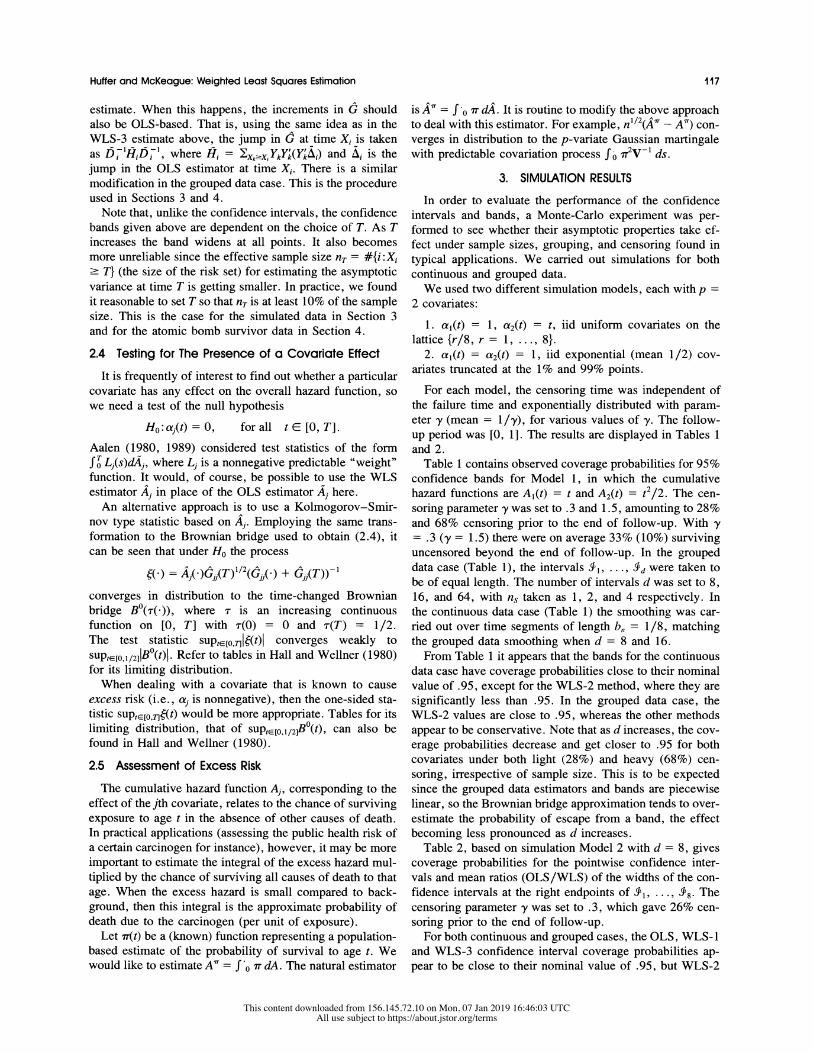
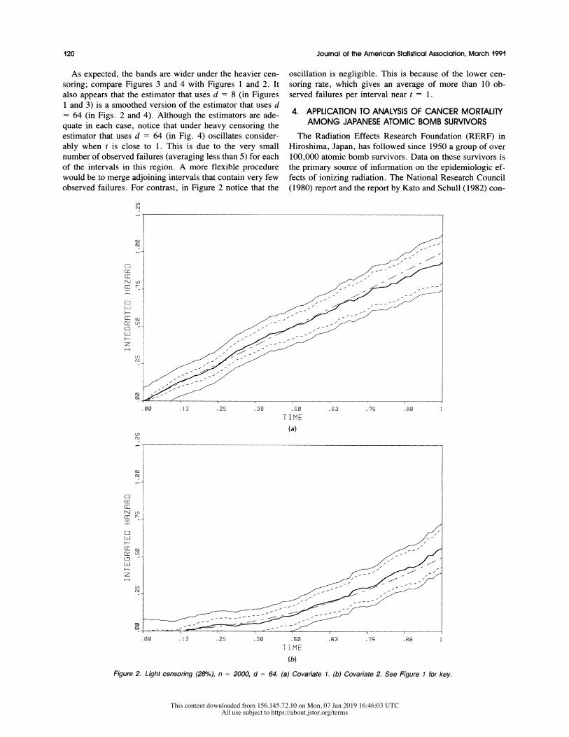
Figure 1. Light censoring (280%), n = 2000, d = 8. (a) Covariate 1. (b) Covariate 2. Thick lines = WLS estimator, regular dashed lines= 95%1 pointwise confidence limits (WLS- 1); thin lines = 95%1 confidence bands (WLS- 1); irregular dashed lines = true cumulative hazard functions (Figs. 1-4).



As expected, the bands are wider under the heavier cen-

soring; compare Figures 3 and 4 with Figures 1 and 2. It

also appears that the estimator that uses d = 8 (in Figures

1 and 3) is a smoothed version of the estimator that uses d

= 64 (in Figs. 2 and 4). Although the estimators are ade-

quate in each case, notice that under heavy censoring the

estimator that uses d = 64 (in Fig. 4) oscillates consider-

ably when t is close to 1. This is due to the very small

number of observed failures (averaging less than 5) for each

of the intervals in this region. A more flexible procedure

would be to merge adjoining intervals that contain very few

observed failures. For contrast, in Figure 2 notice that the

oscillation is negligible. This is because of the lower cen-

soring rate, which gives an average of more than 10 ob-

served failures per interval near t = 1.

4. APPLICATION TO ANALYSIS OF CANCER MORTALITY AMONG JAPANESE ATOMIC BOMB SURVIVORS

The Radiation Effects Research Foundation (RERF) in

Hiroshima, Japan, has followed since 1950 a group of over

100,000 atomic bomb survivors. Data on these survivors is

the primary source of information on the epidemiologic ef-

fects of ionizing radiation. The National Research Council

(1980) report and the report by Kato and Schull (1982) con-

CET

N4 U)

Li:

CED

I

H-D

ci:

. 00 . 13 .25 .38 . 50 .63 .75 .88 I

(a)

F r_-

U-) N -

.00 .13 .25 .38 .50 .G3 .75 .88

(a)

Fiure2)ih esrn 20o,n 20,d=6.()Coait .)Cvrae2 e iue1frky



tain detailed analyses of these data. As noted by Pierce and Preston (1984), however, a difficulty with the methods used in these reports is that they do not make explicit allowance

for temporal variation in risks; they simply average the risk over the follow-up period.

Pierce and Preston (1985) studied cancer mortality among the atomic bomb survivors using a parametric additive risk

model. They found that background and excess rates of cancer mortality vary markedly with age at exposure and time since exposure.

We fitted the additive risk model (1.1) to the data used by Pierce and Preston (1985). We analyzed separately each

of 4 cohorts defined by the age at exposure intervals 0-9,

10-19, 20-34, and 35-49 years of age at time of bomb.

The time variable t is time since exposure, ranging from 5

to 37 years over the follow-up period, 1950-1982. The only

censoring prior to the end of follow-up is that due to other

(noncancer) causes of death. Summary information for each

cohort is given in Table 3. Further description of the data

can be found in Preston, Kato, Kopecky, and Fujita (1986).

Three covariates are used. For individual i they are: Yi1 = indicator (male), Yi2 =indicator (female), Yi3 = dose (in units of 100 rads). The hazard functions a, and a2 are the background cancer mortality rates for males and females

LO

CE:

CE: ~ ~ ~ ~ ~ ~ ~ TM

C-D

LU(

r S

. 00 . 13 .25 .38 . 50 .63 .75 .88 1

(a)

F r_-

Hr-

z-L

c-i:

LU

LIS

.00 .13 .25 .38 .50 .63 .75 .88 I

(b)

Figure 3. Heavy censoring (680%), n =2000, d =8. (a) Covariate L. (b) Covariate 2. See Figure 1 for key.



respectively. The third hazard function a3 iS the excess can-

cer mortality rate per 100 rads of radiation exposure.

In the data provided to us by the RERF, time since ex-

posure is grouped into eight 4-year intervals: 5-9,

33-37 years. It is natural to use these eight time intervals

as the partition of the follow-up period in the evaluation of

the WLS estimator. The Monte Carlo study in Section 3

indicates that satisfactory results can be obtained with as

few as d = 8 intervals. As in Pierce and Preston (1985), the dose variable is taken as the midpoint of one of the six

Table 3. Cohort Sizes, Summary Mortality Figures, and Censoring Prior to End of Follow-up

Deaths due to Age at cancer excluding Deaths from

exposure Cohort size* leukemia all causes Censoring

0-9 18,416 93 728 87% 10-19 19,242 349 1,715 80% 20-34 17,694 949 3.075 69% 35-49 20,916 2,788 11,234 75%

*Approximate, having been estimated from the grouped data.

LO

C:

CE:

CD

LO

.0 . 1 3 .25 .38 . 50 .63 . 75 .88 I

T I M E

(a) F-

(\1~~~~~~~~~~~~~~b ig 4: H F

ct u) _

ZC __ D~?

.00 .13 .25 .38 .50 .63 .75 .88 1

TIME

(a)

i ure4 ev esrn 6%,n=20,d=6.()Coait .()Cvrae2 e iue1frky



dose groups: 0, 1-50, 50-100, 100-200, 200 -300, >300

rads with dose = 400 for dose > 300. The data used here

are based on the old dosimetry, T65DR. The analysis is

limited to the epithelial cancer mortality, in which leukemia

mortality is excluded. We use ns = 1; that is, the weights are calculated using the OLS estimator for only the pre-

vious interval, and the variance estimator is WLS-1.

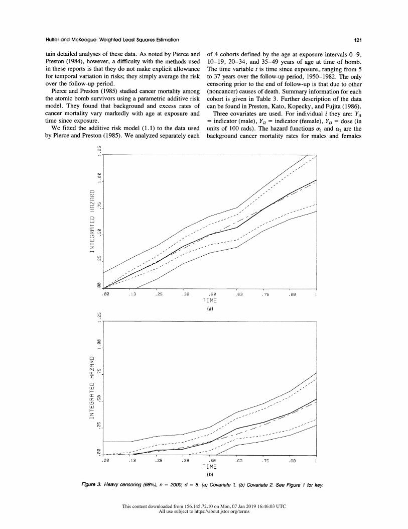
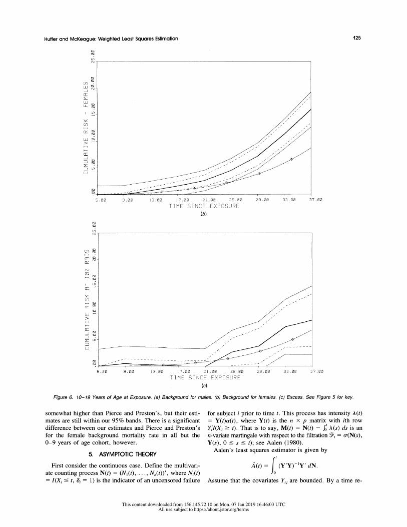
Figures 5-8 indicate our estimates and 95% confidence

intervals and bands for the background and excess cumu-

lative cancer mortality rates as functions of time since ex-

posure. The estimates of Pierce and Preston are also plot-

ted. All estimates are given in units of deaths per 1,000

persons at risk. Pierce and Preston's parametric model for

the cancer mortality rate A(t) is given by

A(t) = exp{voe + vl, + v2, log(e + t)}

+ I3dexp{poe + p, log(t)}, (4.1)

where e = midpoint of age at exposure interval, s = sex,

and d = dose. The first and second terms in (4. 1) represent

the background and excess cancer mortality rates which

Pierce and Preston fitted by maximum likelihood. We have

n

cn Li

I

CE cn

Li

-J

5 .00 9 .00 1 3. 00 1 7 .00 2 1 .00 25 .00 29 .00 33 .00 37 .00

TIME SINCF EXPOSURE

(a)

Co

LU

1 CE

H-

cr ~-J

L -

CO

GU <

Co

D o-- - =__ ------_ . -_ _

5.00 9.00 13.00 17.00 21.00 25.00 29.00 33.00 37.00 TIME SINCE EXPOSURE

(b)

Figure 5. (continlued)



G 0?

C:)

CL

cn

CL:

5.00 9.00 13.00 17.00 21.00 25.00 29.00 33.00 37.00

TIME SINCE EXPOSURE

(c)

Figure 5. 0-9 Years of Age at Exposure. (a) Background for males. (b) Background for females. (c) Excess. Thick lines = WLS estimator; regular dashed lines = 95% pointwise confidence limits (WLS-1); thin lines = 95% confidence bands (WLS-1); lines marked with boxes = estimates of Pierce and Preston (Figs. 5-8).

integrated these to provide a comparison with our WLS es-

timates.

From Figures 5-8 we see that there is a significant dose

effect (since the band for dose does not contain the zero

function) for all cohorts. This is despite the fact that the

confidence bands with d = 8 are conservative according to

our simulation results in Section 3. In interpreting Figures

5-8, bear in mind that the vertical scales are different for

each cohort. Despite appearances, the dose effect bands have

roughly the same width for each cohort.

On the whole, our estimates are in agreement with those

of Pierce and Preston (1985). We also observe that the rel-

ative risk (dose effect vs. background) decreases sharply

with age at exposure. Our estimates for the dose effect are

LO

G / LiC

U)~~~~~~~~~~~~~~~a

F-F

LO

0.00 9.00 13.00 17.00 21.00 25.00 29.00 33.00 37.00

TIME SINCE EXPOSLURE

(a)

Figure 6. (continued)



LO (n -

LU l

Li

CLU

LUJ

H-

LU0

5.00 8.00 13.00 17.00 21.00 25.00 29.00 33.00 37.00

TIME SINCE EXPOSURE

(b)

Ln

(-in

Li

CH-

LU0

5.00 9.00 13.00 17.00 21.00 25.00 29.00 33.00 37.00

TIME SINCE EXPOSURE

(c)

Figure 6. 10-19 Years of Age at Exposure. (a) Background for males. (b) Background for females. (c) Excess. See Figure 5 for key.

somewhat higher than Pierce and Preston's, but their esti-

mates are still within our 95% bands. There is a significant

difference between our estimates and Pierce and Preston's

for the female background mortality rate in all but the

0-9 years of age cohort, however.

5. ASYMPTOTIC THEORY

First consider the continuous case. Define the multivari-

ate counting process N(t) = (NI(t), ..., Nn(t))', where Ni(t) = I(Xi < t, Si = 1) is the indicator of an uncensored failure

for subject i prior to time t. This process has intensity A(t)

= Y(t)a(t), where Y(t) is the n x p matrix with ith row

Yi'I(Xi ' t). That is to say, M(t) = N(t) - fo A(s) ds is an n-variate martingale with respect to the filtration J;t = o-(N(s), Y(s), 0 ' s ' t); see Aalen (1980).

Aalen's least squares estimator is given by

A(t) = (Y'Y)y -Y' dN.

Assume that the covariates Yij are bounded. By a time re-



versed version of Ranga Rao's (1962) law of large num-

bers, the p x p miatrices n-1Y'Y, n-1Y'(diag Ya)Y con-

verge uniformly on [0, T], in probability, to deterministic

limits. Here diag Ya is the diagonal matrix having diagonal

Ya. Assume that the limit of n-1Y'Y is nonsingular and

continuous (or, more generally, has smallest eigenvalue

bounded away from zero) on [0, T]. Then A - A coincides

in probability, as n -- oo, with the p-variate martingale M = ?(Y'Y)Y1Y' dM. Now, M has predictable covariation process

)=t (YY)Y lY'(diag Ya)Y(Y'Y)- ds,

so that (n'/2M* converges pointwise in probability to a continuous deterministic function. The maximum jump of

n1/2M is Op(n-1/2). Thus Rebolledo's (1980) martingale central limit theorem implies that n"/2M [and hence n"/2 (A - A)] converges in distribution to a p-variate continuous

Gaussian martingale. In particular, if bn -* O and nbn -? cc, then the smoothed least squares estimator given by (2.3) is

cLJ-

5.00 9.00 13.00 17.00 21.00 25.00 29.00 33.00 37.00

TIME SINCE EXPOSURE

(a)

n-

11 s

L, Si

LL I

5.00 9.00 13.00 17.00 21.00 25.00 29.00 33.00 37.00

TIME SINCE EXPOSURE

(b)




clc

Hn

cLO

5.00 9.00 13.00 17.00 21.00 25.00 29.00 33.00 37.00 T IME SI NCE EXPOSURE

(c)


uniformly consistent over [b, T]; see the proof of Theorem 4.1.2 of Ramlau-Hansen (1983).

Next consider the WLS estimator

A(t) = (Y'WY)-1Y'W dN,

where W = (diag Ya*)-l and a* is the kernel estimator

(2.3). In practice, we use the WLS estimator on [b, T] and

the OLS estimator on [0, b]. Note that, since bn -* 0, this modification has no effect asymptotically. Assume that the

intensity Ai(t) of Ni is uniformly bounded away from zero

unless Yij(t) = 0 for all j = 1, . . ., p. Then W is a uniformly consistent estimator of the "true" weight W = (diag

Ya) 1 over [b, T]. To simplify the notation, assume from

(9

cn

CD)

-

5.00 9.00 13.00 17.00 21.00 25.00 29.00 33.00 37.00

T IME SI NCE EXPOSURE

(a)




L,J-

LLi ("

CE

LL D

-

E)-

L--i Co

H-

cF--

G-

9.00 9.00 13.00 17.00 21.00 25.00 29.00 33.00 37.00

TIME SINGE EXPOSURE

(b)

U-)

a: H -

C S

CO

\-

9.00 9.00 13.00 17.00 21.00 29.00 29.00 33.00 37.00

T IME SI NGE EXPOSURE

(c)


now on that this is so over the whole of [0, T]. Using Ranga Rao's (1962) law of large numbers again, we have that

n-'Y'WY converges uniformly in probability on [0, T] to a deterministic matrix function V. By uniform consistency of W and boundedness of the covariates, n Y'WY also

converges uniformly in probability on [0, T] to V. Assume

that V is nonsingular and smooth on [0, T]. Then A - A coincides in probability, as n co), with M = ?(Y'WYY1Y'W dM, which is a p-variate martingale, since

W was arranged to be predictable. Moreover,

( t (Y WY) Y'W(diag Ya)WY(Y'WY) ds,

so that (n 1I2M), converges in probability to Jt-V ds. Thus Rebolledo's (1980) martingale central limit theorem im-

plies that n'12(A - A) converges in distribution to a p-variate Gaussian martingale with predictable covariation process


weighted least squares estimation for - columbia universityim2131/ps/huffmckjasa.pdf · weighted...

Documents