week 5 linear algebra i

AMATH 460: Mathematical Methodsfor Quantitative Finance

5. Linear Algebra I

Kjell KonisActing Assistant Professor, Applied Mathematics

University of Washington

Kjell Konis (Copyright © 2013) 5. Linear Algebra I 1 / 68

Outline

1 Vectors

2 Vector Length and Planes

3 Systems of Linear Equations

4 Elimination

5 Matrix Multiplication

6 Solving Ax = b

7 Inverse Matrices

8 Matrix Factorization

9 The R Environment for Statistical Computing


Outline

1 Vectors



4 Elimination


6 Solving Ax = b

7 Inverse Matrices




Vectors

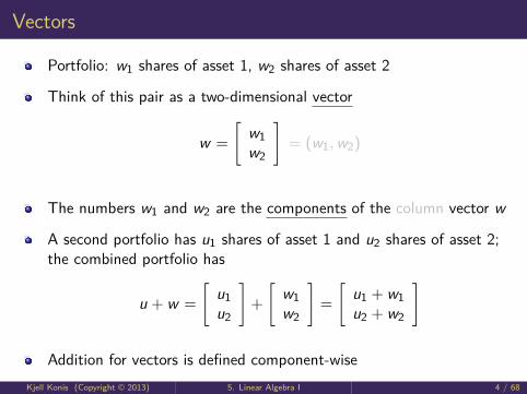
Portfolio: w1 shares of asset 1, w2 shares of asset 2

Think of this pair as a two-dimensional vector

w =

[w1w2

]= (w1,w2)

The numbers w1 and w2 are the components of the column vector w

A second portfolio has u1 shares of asset 1 and u2 shares of asset 2;the combined portfolio has

u + w =

[u1u2

]+

[w1w2

]=

[u1 + w1u2 + w2

]

Addition for vectors is defined component-wiseKjell Konis (Copyright © 2013) 5. Linear Algebra I 4 / 68

Vectors

Doubling a vector

2w = w + w =

[w1w2

]+

[w1w2

]=

[w1 + w1w2 + w2

]=

[2w12w2

]

In general, multiplying a vector by a scalar value c

cw =

[cw1cw2

]

A linear combination of vectors u and w

c1u + c2w =

[c1u1c1u2

]+

[c2w1c2w2

]=

[c1u1 + c2w1c1u2 + c2w2

]

Setting c1 = 1 and c2 = −1 gives vector subtraction

u − w = 1u +−1w =

[1u1 +−1w11u2 +−1w2

]=

[u1 − w1u2 − w2

]Kjell Konis (Copyright © 2013) 5. Linear Algebra I 5 / 68

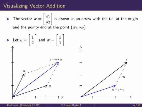
Visualizing Vector Addition

The vector w =

[w1w2

]is drawn as an arrow with the tail at the origin

and the pointy end at the point (w1,w2)

Let u =

[12

]and w =

[31

]

w

u

v = w + u v

w = v − u

−u


Vector Addition

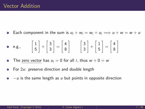
Each component in the sum is ui + wi = wi + ui =⇒ u + w = w + u

e.g.,[

15

]+

[33

]=

[48

] [33

]+

[15

]=

[48

]

The zero vector has ui = 0 for all i , thus w + 0 = w

For 2u: preserve direction and double length

−u is the same length as u but points in opposite direction


Dot Products

The dot product or inner product of u = (u1, u2) and w = (w1,w2) isthe scalar quantity

u · w = u1w1 + u2w2

Example: letting u = (1, 2) and w = (3, 1) gives

u · v = (1, 2) · (3, 1) = 1× 3 + 2× 1 = 5

Interpretation:w is a position in assets 1 and 2Let p = (p1, p2) be the prices of assets 1 and 2

V = w · p = w1p1 + w2p2

value of portfolioKjell Konis (Copyright © 2013) 5. Linear Algebra I 8 / 68

Outline

1 Vectors



4 Elimination


6 Solving Ax = b

7 Inverse Matrices




Lengths

The length of a vector w is

length(w) = ‖w‖ =√

w · w

Example: suppose w = (w1,w2,w3,w4) has 4 components

‖w‖ =√

w · w =√

w21 + w2

2 + w23 + w2

4

The length of a vector is positive except for the zero vector, where

‖0‖ = 0

A unit vector is a vector whose length is equal to one: u · u = 1

A unit vector having the same direction as w 6= 0

w =w‖w‖


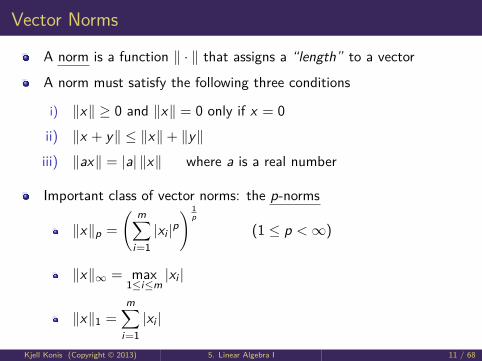
Vector Norms

A norm is a function ‖ · ‖ that assigns a “length” to a vector

A norm must satisfy the following three conditions

i) ‖x‖ ≥ 0 and ‖x‖ = 0 only if x = 0

ii) ‖x + y‖ ≤ ‖x‖+ ‖y‖

iii) ‖ax‖ = |a| ‖x‖ where a is a real number

Important class of vector norms: the p-norms

‖x‖p =

( m∑i=1|xi |p

) 1p

(1 ≤ p <∞)

‖x‖∞ = max1≤i≤m

|xi |

‖x‖1 =m∑

i=1|xi |


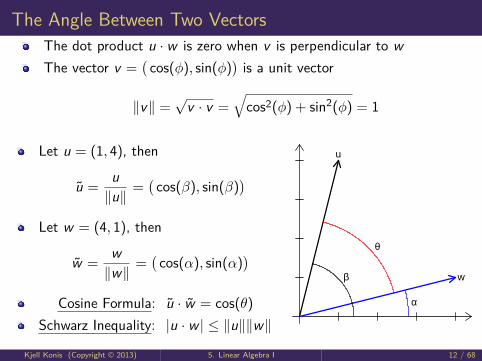
The Angle Between Two VectorsThe dot product u · w is zero when v is perpendicular to wThe vector v =

(cos(φ), sin(φ)

)is a unit vector

‖v‖ =√

v · v =√

cos2(φ) + sin2(φ) = 1

Let u = (1, 4), then

u =u‖u‖ =

(cos(β), sin(β)

)Let w = (4, 1), then

w =w‖w‖ =

(cos(α), sin(α)

)Cosine Formula: u · w = cos(θ)

Schwarz Inequality: |u · w | ≤ ‖u‖‖w‖

u

w

α

β

θ


Planes

So far, 2-dimensionalEverything (dot products, lengths, angles, etc.) works in higherdimensions tooA plane is a 2-dimensional sheet that lives in 3 dimensionsConceptually, pick a normal vector n and define the plane P to be allvectors perpendicular to nIf a vector v = (x , y , z) ∈ P then

n · v = 0

However, since n · 0 = 0, 0 ∈ PThe equation of the plane passing through v0 = (x0, y0, z0) andnormal to n is

n · (v − v0) = n1(x − x0) + n2(y − y0) + n3(z − z0) = 0


Planes (continued)

Every plane normal to n has a linear equation withcoefficients n1, n2, n3:

n1x + n2y + n3z = n1x0 + n2y0 + n3z0 = d

Different values of d give parallel planesThe value d = 0 gives a plane through the origin


Outline

1 Vectors



4 Elimination


6 Solving Ax = b

7 Inverse Matrices




Systems of Linear Equations

Want to solve 3 equations in 3 unknownsx + 2y + 3z = 6

2x + 5y + 2z = 46x − 3y + z = 2

Row picture:(1, 2, 3) · (x , y , z) = 6(2, 5, 2) · (x , y , z) = 4

(6,−3, 1) · (x , y , z) = 2

Column picture:

x

126

+ y

25−3

+ z

321

=

642


Systems of Linear Equations

28 I Vectors and Matrices 1.4 Matrices and Linear Equations

The central problem of linear algebra is to solve linear equations. There are twoways to describe that problem—first by rows and then by colunins. In this chapter weexplain the problem. in the next chapter we solve it.Start with a system of three equations in th:’ee unknowns. Let the unknowns be

x. u.;. and let the linear equations be

x ± 2*’ + 3; 6Iv - 5v + 2; = 46x

—3; ± ; 2.

We look for numbers x. v,; that solve all three equations at once. Those numbersmight or might not exist. For this system, they do exist. When the number ofequations matches the number of unknowns, there is usually one solution. Theimmediate problem is how to visualize the three equations. There is a row pictureand a column picture.R The row picture shows three planes meeting at a single point.

The first plane comes from the first equation x ± 2v 3; = 6. That plane crosses thex.y,; axes at (6,0,0) and (0.3,0) and (0.0,2). The plane does not go through theorigin - —the right side of its equation is 6 and not zero.The second plane is given by the equation 2.v + 5i -i- 2; 4 from the second row.

The numbers 0. 0, 2 satisfy both equations, so the point (0,0. 2) lies on both planes.Those two planes intersect in a line L, which goes through (0.0,2).The third equation gives a third plane. It cuts the line L at a single point. That

point lies on all three planes. This is the row picture of equation (1)- three planesmeeting at a single point (x.v,;). The numbers x,y.; solve all three equations.

Figure 1.12 Column picture of three equations: Combinations of columns areb 2> column 3 so (x.v. = (0.0. 2) b = sum of columns so (x.i-.:) = (1. 1. 1).

C The column picture combines the columns on the left side to produce the right side.Write the three equations as one vector equation based on columns:

3 6+z 2 = 4

2

The row picture has planes given by dot products. The column picture has this linearcombination. The unknown numbers .v. v. = are the coefficients in the combination.We multiply the columns by the correct numbers x.y.; to give the column (6,4.2).For this particular equation I know the right combination (I made up the problem).

If x and v are zero, and = equals 2. then 2 times the third column agrees with thecolumn on the right. The solution is -v = 0. i’ = 0. 2. That point (0.0,2) lies onall three planes in the row picture. It solves all three equations. The row and columnpictures show the same solution in different ways.For one moment. change to a new right hand side (6.9.4). This vector equals

column 1 + column 2 + column 3. The solution with this new right hand side is(x.v. =

_______.

The numbers x. i. z multiply the columns to give b.

We have three rows in the row picture and three columns in the column picture(plus the right side). The three rows and columns contain nine numbers. These ninenumbers fill a 3 hi 3 matrix. We are coming to the matrix picture. The “coefficientmatrix” has the rows and columns that have so far been kept separate:

‘12i6J

29

(I)

cot I

2

—3

± cot 3

cot 2

[] +4 5 (2)

1 2 3The coefficient matrix is A 2 5 2

6 —3 1Figure 1.11 Row picture of three equations: Three planes meet at a point.


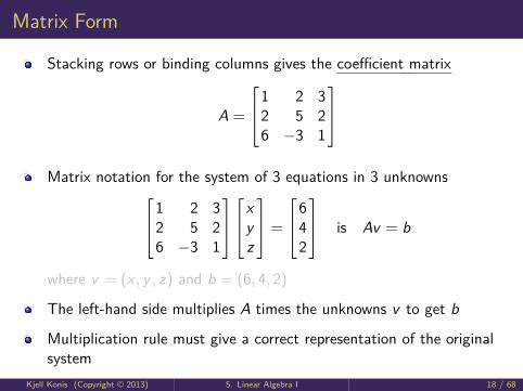
Matrix Form

Stacking rows or binding columns gives the coefficient matrix

A =

1 2 32 5 26 −3 1

Matrix notation for the system of 3 equations in 3 unknowns1 2 3

2 5 26 −3 1

x

yz

=

642

is Av = b

where v = (x , y , z) and b = (6, 4, 2)

The left-hand side multiplies A times the unknowns v to get b

Multiplication rule must give a correct representation of the originalsystem


Matrix-Vector Multiplication

Row picture multiplication

Av =

(row 1) · v(row 2) · v(row 3) · v

=

(row 1) · (x , y , z)(row 2) · (x , y , z)(row 3) · (x , y , z)

Column picture multiplication

Av = x (column 1) + y (column 2) + z (column 3)

Examples:

Av =

1 0 01 0 01 0 0

4

56

=

444

Av =

1 0 00 1 00 0 1

4

56

=

456


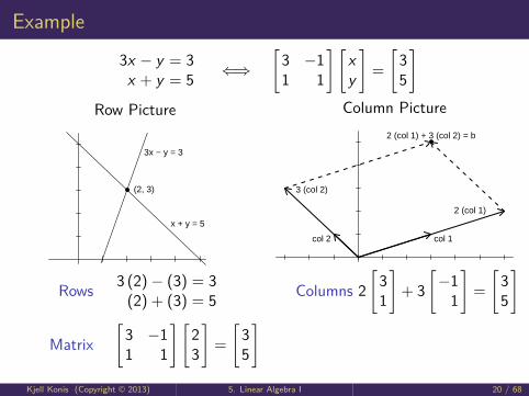
Example

3x − y = 3x + y = 5 ⇐⇒

[3 −11 1

] [xy

]=

[35

]Row Picture

● (2, 3)

x + y = 5

3x − y = 3

Rows 3 (2)− (3) = 3(2) + (3) = 5

Column Picture

col 2

3 (col 2)

col 1

2 (col 1)

●2 (col 1) + 3 (col 2) = b

Columns 2[

31

]+ 3

[−1

1

]=

[35

]

Matrix[

3 −11 1

] [23

]=

[35


Systems of Equations

For an equal number of equations and unknowns, there is usually onesolution

Not guaranteed, in particular there may beno solution (e.g., when the lines are parallel)infinitely many solutions (e.g., two equations for the same line)


Outline

1 Vectors



4 Elimination


6 Solving Ax = b

7 Inverse Matrices




Elimination

Want to solve the system of equations

x − 2y = 13x + 2y = 11

High school algebra approachsolve for x : x = 2y + 1eliminate x : 3(2y + 1) + 2y = 11solve for y : 8y + 3 = 11 =⇒ y = 1solve for x : x = 3


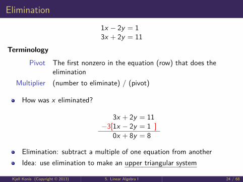
Elimination

1x − 2y = 13x + 2y = 11

Terminology

Pivot The first nonzero in the equation (row) that does theelimination

Multiplier (number to eliminate) / (pivot)

How was x eliminated?

3x + 2y = 11−3[1x − 2y = 1 ]

0x + 8y = 8

Elimination: subtract a multiple of one equation from anotherIdea: use elimination to make an upper triangular system


Elimination

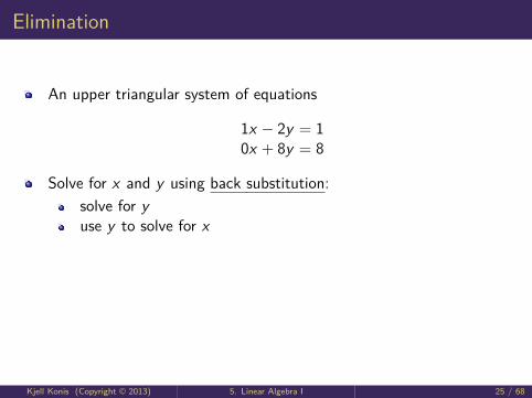
An upper triangular system of equations

1x − 2y = 10x + 8y = 8

Solve for x and y using back substitution:solve for yuse y to solve for x


Elimination Using Matrices

The system of 3 equations in 3 unknowns can be written in thematrix form Ax = b

2x1 + 4x2 − 2x3 = 24x1 + 9x2 − 3x3 = 8−2x1 − 3x2 + 7x3 = 10

∼

2 4 −24 9 −3−2 −3 7

︸︷︷︸

A

x1x2x3

︸︷︷︸

x

=

28

10

︸︷︷︸

b

The unknown is

x1x2x3

and the solution is

−122

Ax = b represents the row form and the column form of the systemCan multiply Ax a column at a time

Ax = (−1)

24−2

+ 2

49−3

+ 2

−2−3

7

=

28

10


Elimination Using Matrices

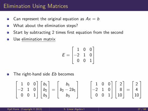
Can represent the original equation as Ax = bWhat about the elimination steps?Start by subtracting 2 times first equation from the secondUse elimination matrix

E =

1 0 0−2 1 0

0 0 1

The right-hand side Eb becomes 1 0 0−2 1 0

0 0 1

b1

b2b3

=

b1b2 − 2b1

b3

1 0 0−2 1 0

0 0 1

2

810

=

24

10


Two Important Matrices

The identity matrix has 1’s on the diagonal and 0’s everywhere else

I =

1 0 00 1 00 0 1

The elimination matrix that subtracts a multiple l of row j from row ihas an additional nonzero entry −l in the i , j position

E3,1(l) =

1 0 00 1 0−l 0 1

Examples

E2,1(2)b =

b1b2 − 2b1

b3

Ib =

1 0 00 1 00 0 1

b1

b2b3

=

b1b2b3


Outline

1 Vectors



4 Elimination


6 Solving Ax = b

7 Inverse Matrices




Matrix Multiplication

Have linear system Ax = b and elimination matrix EOne elimination step (introduce one 0 below the diagonal)

EAx = Eb

Know how to do right-hand-sideSince E is an elimination matrix, also know answer to EAColumn view:

The matrix A is composed of n columns a1, a2, . . . , anThe columns of the product EA are

EA =[Ea1,Ea2, . . . ,Ean

]


Rules for Matrix Operations

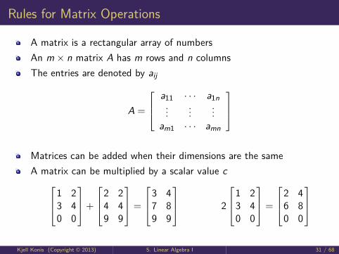
A matrix is a rectangular array of numbersAn m × n matrix A has m rows and n columnsThe entries are denoted by aij

A =

a11 · · · a1n...

......

am1 · · · amn

Matrices can be added when their dimensions are the sameA matrix can be multiplied by a scalar value c1 2

3 40 0

+

2 24 49 9

=

3 47 89 9

2

1 23 40 0

=

2 46 80 0


Rules for Matrix Multiplication

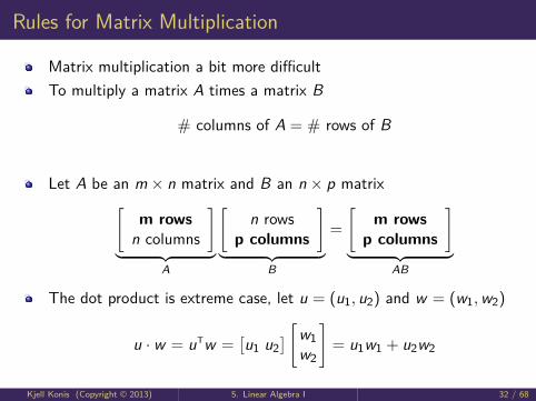
Matrix multiplication a bit more difficultTo multiply a matrix A times a matrix B

# columns of A = # rows of B

Let A be an m × n matrix and B an n × p matrix[m rows

n columns

]︸︷︷︸

A

[n rows

p columns

]︸︷︷︸

B

=

[m rows

p columns

]︸︷︷︸

AB

The dot product is extreme case, let u = (u1, u2) and w = (w1,w2)

u · w = uTw =[u1 u2

] [w1w2

]= u1w1 + u2w2


Matrix Multiplication

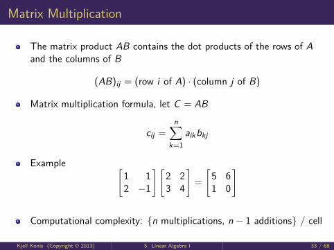
The matrix product AB contains the dot products of the rows of Aand the columns of B

(AB)ij = (row i of A) · (column j of B)

Matrix multiplication formula, let C = AB

cij =n∑

k=1aikbkj

Example [1 12 −1

] [2 23 4

]=

[5 61 0

]

Computational complexity: {n multiplications, n − 1 additions} / cell


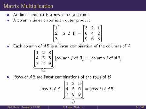
Matrix MultiplicationAn inner product is a row times a columnA column times a row is an outer product1

23

[3 2 1]=

3 2 16 4 29 6 3

Each column of AB is a linear combination of the columns of A1 2 3

4 5 67 8 9

︸︷︷︸

A

[column j of B

]=[column j of AB

]

Rows of AB are linear combinations of the rows of B

[row i of A

] 1 2 34 5 67 8 9

︸︷︷︸

B

=[row i of AB

]


Laws for Matrix Operations

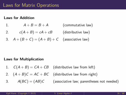
Laws for Addition

1. A + B = B + A (commutative law)

2. c(A + B) = cA + cB (distributive law)

3. A + (B + C) = (A + B) + C (associative law)

Laws for Multiplication

1. C(A + B) = CA + CB (distributive law from left)

2. (A + B)C = AC + BC (distributive law from right)

3. A(BC) = (AB)C (associative law; parentheses not needed)


Laws for Matrix Operations

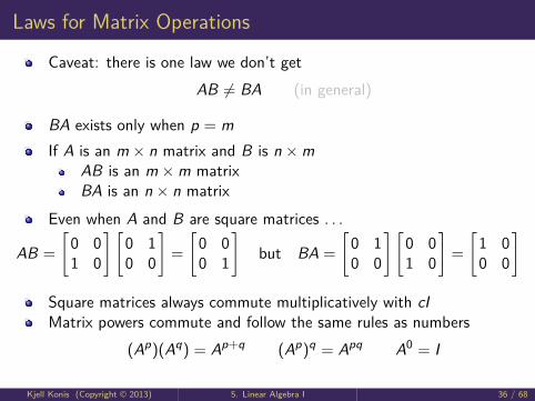
Caveat: there is one law we don’t getAB 6= BA (in general)

BA exists only when p = mIf A is an m × n matrix and B is n ×m

AB is an m ×m matrixBA is an n × n matrix

Even when A and B are square matrices . . .

AB =

[0 01 0

] [0 10 0

]=

[0 00 1

]but BA =

[0 10 0

] [0 01 0

]=

[1 00 0

]

Square matrices always commute multiplicatively with cIMatrix powers commute and follow the same rules as numbers

(Ap)(Aq) = Ap+q (Ap)q = Apq A0 = I


Block Matrices/Block Multiplication

A matrix may be broken into blocks (which are smaller matrices)

A =

1 0 1 0 1 00 1 0 1 0 11 0 1 0 1 00 1 0 1 0 1

=

[I I II I I

]

Addition/multiplication allowed when block dimensions appropriate[A11 A12A21 A22

] [B11 . . .

B21 . . .

]=

[A11B11 + A12B21 . . .

A21B11 + A22B21 . . .

]

Let the blocks of A be its columns and the blocks of B be its rows

AB =

| |a1 · · · an| |

︸︷︷︸

m×n

— b1 —...

— bn —

︸︷︷︸

n×p

=n∑

i=1

aibi

︸︷︷︸

m×p


Outline

1 Vectors



4 Elimination


6 Solving Ax = b

7 Inverse Matrices




Elimination in Practice

Solve the following system using elimination

2x1 + 4x2 − 2x3 = 24x1 + 9x2 − 3x3 = 8−2x1 − 3x2 + 7x3 = 10

2 4 −24 9 −3−2 −3 7

x1

x2x3

=

28

10

Augment A: the augmented matrix A′ is

A′ =[A b

]=

2 4 −2 24 9 −3 8−2 −3 7 10

Strategy: find the pivot in the first row and eliminate the valuesbelow it


Example (continued)

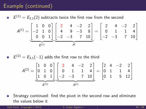
E (1) = E2,1(2) subtracts twice the first row from the second

A(1) =

1 0 0−2 1 0

0 0 1

︸︷︷︸

E (1)

2 4 −2 24 9 −3 8−2 −3 7 10

︸︷︷︸

A′

=

2 4 −2 20 1 1 4−2 −3 7 10

E (2) = E3,1(−1) adds the first row to the third

A(2) =

1 0 00 1 01 0 1

︸︷︷︸

E (2)

2 4 −2 20 1 1 4−2 −3 7 10

︸︷︷︸

A(1)

=

2 4 −2 20 1 1 40 1 5 12

Strategy continued: find the pivot in the second row and eliminatethe values below it


Example (continued)

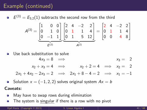
E (3) = E3,2(1) subtracts the second row from the third

A(3) =

1 0 00 1 00 −1 1

︸︷︷︸

E (3)

2 4 −2 20 1 1 40 1 5 12

︸︷︷︸

A(2)

=

2 4 −2 20 1 1 40 0 4 8

Use back substitution to solve4x3 = 8 =⇒ x3 = 2

x2 + x3 = 4 =⇒ x2 + 2 = 4 =⇒ x2 = 22x1 + 4x2 − 2x3 = 2 =⇒ 2x1 + 8− 4 = 2 =⇒ x1 = −1

Solution x = (−1, 2, 2) solves original system Ax = bCaveats:

May have to swap rows during eliminationThe system is singular if there is a row with no pivot


Outline

1 Vectors



4 Elimination


6 Solving Ax = b

7 Inverse Matrices




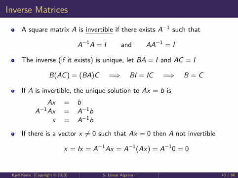
Inverse Matrices

A square matrix A is invertible if there exists A−1 such that

A−1A = I and AA−1 = I

The inverse (if it exists) is unique, let BA = I and AC = I

B(AC) = (BA)C =⇒ BI = IC =⇒ B = C

If A is invertible, the unique solution to Ax = b isAx = b

A−1Ax = A−1bx = A−1b

If there is a vector x 6= 0 such that Ax = 0 then A not invertible

x = Ix = A−1Ax = A−1(Ax) = A−10 = 0


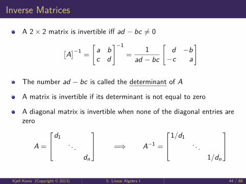
Inverse Matrices

A 2× 2 matrix is invertible iff ad − bc 6= 0

[A]−1

=

[a bc d

]−1=

1ad − bc

[d −b−c a

]

The number ad − bc is called the determinant of A

A matrix is invertible if its determinant is not equal to zero

A diagonal matrix is invertible when none of the diagonal entries arezero

A =

d1. . .

dn

=⇒ A−1 =

1/d1. . .

1/dn


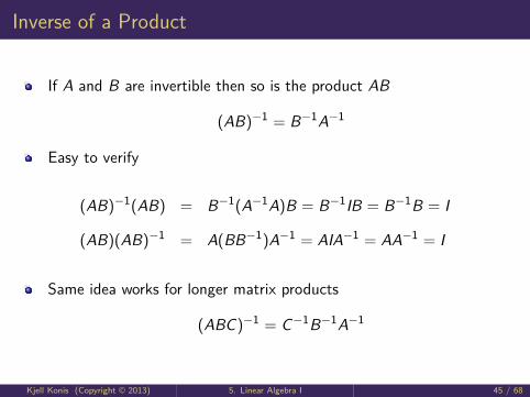
Inverse of a Product

If A and B are invertible then so is the product AB

(AB)−1 = B−1A−1

Easy to verify

(AB)−1(AB) = B−1(A−1A)B = B−1IB = B−1B = I

(AB)(AB)−1 = A(BB−1)A−1 = AIA−1 = AA−1 = I

Same idea works for longer matrix products

(ABC)−1 = C−1B−1A−1


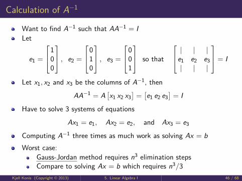
Calculation of A−1

Want to find A−1 such that AA−1 = ILet

e1 =

100

, e2 =

010

, e3 =

001

so that

| | |e1 e2 e3| | |

= I

Let x1, x2 and x3 be the columns of A−1, then

AA−1 = A[x1 x2 x3

]=[e1 e2 e3

]= I

Have to solve 3 systems of equations

Ax1 = e1, Ax2 = e2, and Ax3 = e3

Computing A−1 three times as much work as solving Ax = bWorst case:

Gauss-Jordan method requires n3 elimination stepsCompare to solving Ax = b which requires n3/3


Singular versus Invertible

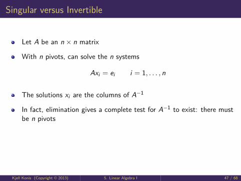
Let A be an n × n matrix

With n pivots, can solve the n systems

Axi = ei i = 1, . . . , n

The solutions xi are the columns of A−1

In fact, elimination gives a complete test for A−1 to exist: there mustbe n pivots


Outline

1 Vectors



4 Elimination


6 Solving Ax = b

7 Inverse Matrices




Elimination = Factorization

Key ideas in linear algebra ∼ factorization of matricesLook closely at 2× 2 case:

E21(3)A =

[1 0−3 1

] [2 16 8

]=

[2 10 5

]= U

E−121 (3)U =

[1 03 1

] [2 10 5

]=

[2 16 8

]= A

Notice E−121 (3) is lower triangular =⇒ call it L

A = LU L lower triangular U upper triangular

For a 3× 3 matrix:(E32 E31 E21

)A = U becomes A =

(E−1

21 E−131 E−1

32)U = LU

(products of lower triangular matrices are lower triangular)Kjell Konis (Copyright © 2013) 5. Linear Algebra I 49 / 68

Seems Too Good To Be True . . . But Is

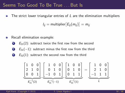
The strict lower triangular entries of L are the elimination multipliers

lij = multiplier[Eij(mij)

]= mij

Recall elimination example:1 E21(2): subtract twice the first row from the second2 E31(−1): subtract minus the first row from the third3 E32(1): subtract the second row from the third

1 0 02 1 00 0 1

︸︷︷︸

E−121 (2)

1 0 00 1 0−1 0 1

︸︷︷︸

E−131 (−1)

1 0 00 1 00 1 1

︸︷︷︸

E−132 (1)

=

1 0 02 1 0−1 1 1

︸︷︷︸

L


One Square System = Two Triangular Systems

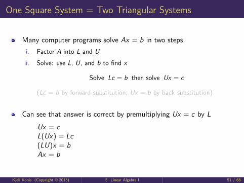
Many computer programs solve Ax = b in two stepsi. Factor A into L and Uii. Solve: use L, U, and b to find x

Solve Lc = b then solve Ux = c

(Lc = b by forward substitution; Ux = b by back substitution)

Can see that answer is correct by premultiplying Ux = c by L

Ux = cL(Ux) = Lc(LU)x = bAx = b


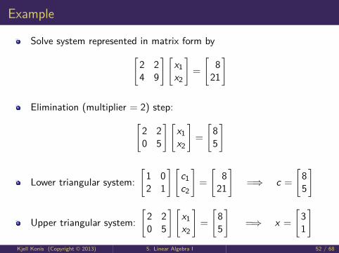
Example

Solve system represented in matrix form by[2 24 9

] [x1x2

]=

[8

21

]

Elimination (multiplier = 2) step:[2 20 5

] [x1x2

]=

[85

]

Lower triangular system:[

1 02 1

] [c1c2

]=

[8

21

]=⇒ c =

[85

]

Upper triangular system:[

2 20 5

] [x1x2

]=

[85

]=⇒ x =

[31


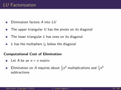
LU Factorization

Elimination factors A into LU

The upper triangular U has the pivots on its diagonal

The lower triangular L has ones on its diagonal

L has the multipliers lij below the diagonal

Computational Cost of Elimination

Let A be an n × n matrix

Elimination on A requires about 13n3 multiplications and 1

3n3

subtractions


Storage Cost of LU Factorization

Suppose we factor

A =

a11 a12 a13a21 a22 a23a31 a32 a33

into

L =

1 0 0l21 1 0l31 l32 1

and U =

d1 u12 u130 d2 u230 0 d3

(d1, d2, d3 are the pivots)

Can write L and U in the space that initially stored A

L and U =

d1 u12 u13l21 d2 u23l31 l32 d3


Outline

1 Vectors



4 Elimination


6 Solving Ax = b

7 Inverse Matrices




The R Environment for Statistical Computing

What is R?R is a language and environment for statistical computing and graphics

R offers: (among other things)

a data handling and storage facilitya suite of operators for calculations on arrays, in particular matricesa well-developed, simple and effective programming language includes

conditionalsloopsuser-defined recursive functionsinput and output facilities

R is free software

http://www.r-project.org


http://www.r-project.org

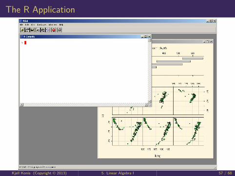
The R Application


R Environment for Statistical Computing

R as a calculator

R commands in the lecture slides look like this> 1 + 1

and the output looks like this[1] 2

When running R, the console will look like this> 1 + 1

[1] 2

Getting help # and commenting your code> help("c") # ?c does the same thing


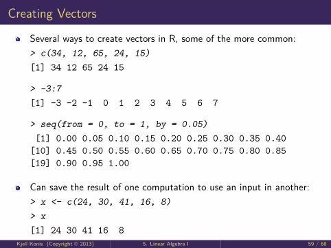
Creating Vectors

Several ways to create vectors in R, some of the more common:> c(34, 12, 65, 24, 15)[1] 34 12 65 24 15

> -3:7[1] -3 -2 -1 0 1 2 3 4 5 6 7

> seq(from = 0, to = 1, by = 0.05)[1] 0.00 0.05 0.10 0.15 0.20 0.25 0.30 0.35 0.40

[10] 0.45 0.50 0.55 0.60 0.65 0.70 0.75 0.80 0.85[19] 0.90 0.95 1.00

Can save the result of one computation to use an input in another:> x <- c(24, 30, 41, 16, 8)> x[1] 24 30 41 16 8


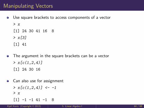
Manipulating Vectors

Use square brackets to access components of a vector> x

[1] 24 30 41 16 8

> x[3]

[1] 41

The argument in the square brackets can be a vector> x[c(1,2,4)]

[1] 24 30 16

Can also use for assignment> x[c(1,2,4)] <- -1> x

[1] -1 -1 41 -1 8Kjell Konis (Copyright © 2013) 5. Linear Algebra I 60 / 68

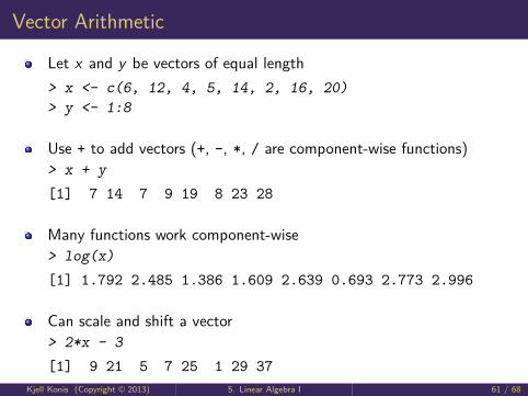
Vector Arithmetic

Let x and y be vectors of equal length> x <- c(6, 12, 4, 5, 14, 2, 16, 20)> y <- 1:8

Use + to add vectors (+, -, *, / are component-wise functions)> x + y

[1] 7 14 7 9 19 8 23 28

Many functions work component-wise> log(x)

[1] 1.792 2.485 1.386 1.609 2.639 0.693 2.773 2.996

Can scale and shift a vector> 2*x - 3

[1] 9 21 5 7 25 1 29 37Kjell Konis (Copyright © 2013) 5. Linear Algebra I 61 / 68

Creating Matrices

Can use the matrix function to shape a vector into a matrix> x <- 1:16> matrix(x, 4, 4)

[,1] [,2] [,3] [,4][1,] 1 5 9 13[2,] 2 6 10 14[3,] 3 7 11 15[4,] 4 8 12 16

Alternatively, can fill in row-by-row> matrix(x, 4, 4, byrow = TRUE)

[,1] [,2] [,3] [,4][1,] 1 2 3 4[2,] 5 6 7 8[3,] 9 10 11 12[4,] 13 14 15 16


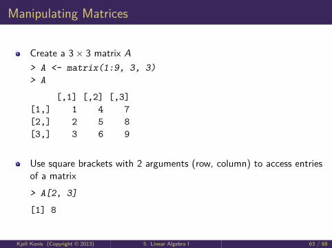
Manipulating Matrices

Create a 3× 3 matrix A> A <- matrix(1:9, 3, 3)> A

[,1] [,2] [,3][1,] 1 4 7[2,] 2 5 8[3,] 3 6 9

Use square brackets with 2 arguments (row, column) to access entriesof a matrix> A[2, 3]

[1] 8


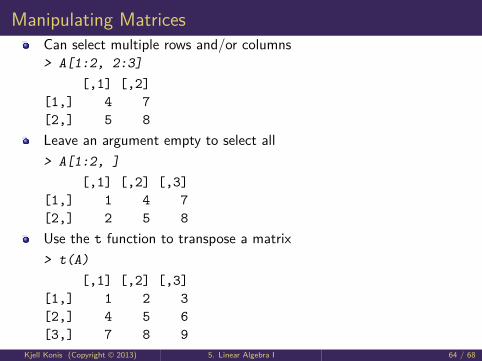
Manipulating MatricesCan select multiple rows and/or columns> A[1:2, 2:3]

[,1] [,2][1,] 4 7[2,] 5 8Leave an argument empty to select all> A[1:2, ]

[,1] [,2] [,3][1,] 1 4 7[2,] 2 5 8Use the t function to transpose a matrix> t(A)

[,1] [,2] [,3][1,] 1 2 3[2,] 4 5 6[3,] 7 8 9


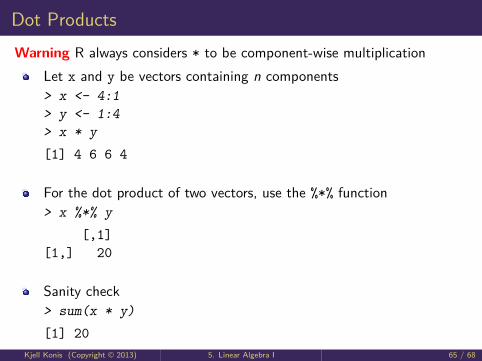
Dot ProductsWarning R always considers * to be component-wise multiplication

Let x and y be vectors containing n components> x <- 4:1> y <- 1:4> x * y

[1] 4 6 6 4

For the dot product of two vectors, use the %*% function> x %*% y

[,1][1,] 20

Sanity check> sum(x * y)

[1] 20Kjell Konis (Copyright © 2013) 5. Linear Algebra I 65 / 68

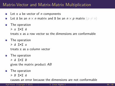
Matrix-Vector and Matrix-Matrix Multiplication

Let x a be vector of n componentsLet A be an n × n matrix and B be an n × p matrix (p 6= n)

The operation> x %*% Atreats x as a row vector so the dimensions are conformable

The operation> A %*% xtreats x as a column vector

The operation> A %*% Bgives the matrix product AB

The operation> B %*% Acauses an error because the dimensions are not conformable


Solving Systems of Equations

Recall the system . . .

x =

−122

solves

2 4 −24 9 −3−2 −3 7

x1

x2x3

=

28

10

Can solve in R using the solve function> A <- matrix(c(2, 4, -2, 4, 9, -3, -2, -3, 7), 3, 3)> b <- c(2, 8, 10)

> solve(A, b)

[1] -1 2 2


http://computational-finance.uw.edu


http://computational-finance.uw.edu

week 5 linear algebra i

Documents

uvu u w w

w c1 u

u w u kjell konis copyright

components w

w kjell konis copyright

vector subtraction u

w wexample

column vector w