MirrorBot

IST-2001-35282

Biomimetic multimodal learning in a mirror neuron-based robot

Cortical assemblies of language areas: Development of cell assembly model for Broca/Wernicke areas

Authors: Andreas Knoblauch, Günther PalmCovering period 1.10.2002-31.8.2003

MirrorBot Prototype 3 (WP 5.2)

Report Version: 1

Report Preparation Date: 31. August 2003

Classification: Restricted

Contract Start Date: 1st June 2002 Duration: Three Years

Project Co-ordinator: Professor Stefan Wermter

Partners: University of Sunderland, Institut National de Recherche en Informatique et en Automatique at Nancy, Universität Ulm, Medical Research Council at Cambridge, Università degli Studi di Parma

Project funded by the European Community under the “Information Society Technologies Programme“

1

Table of Contents

0. Introduction 3

1. Spiking Associative Memory 5

2. Felix++: A tool for implementing cortical areas 7

3. Implementation of cortical language areas 17

4. Test of the model 26

5. Conclusions 30

6. References 31

2

0. Introduction

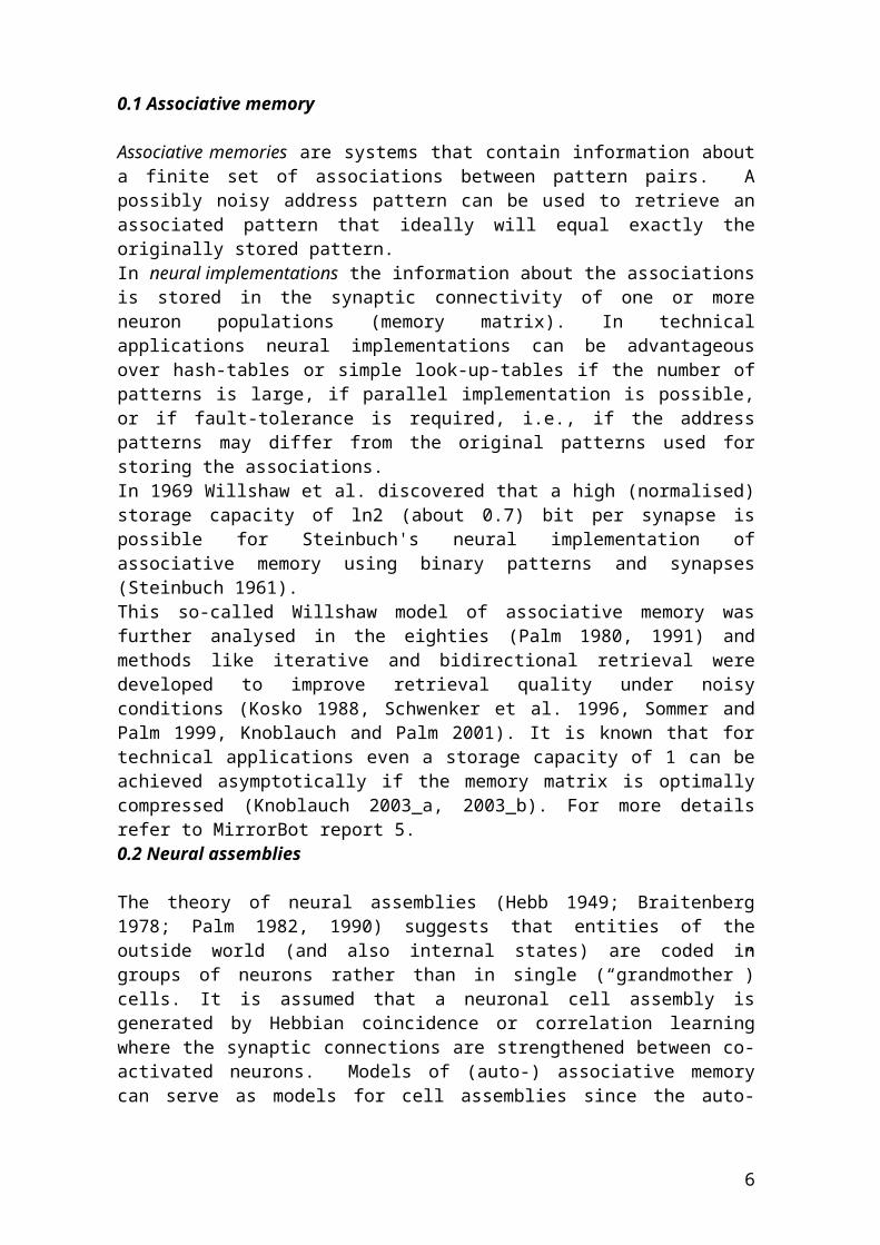
In MirrorBot report 5 (work package 5.1) we have described a model for cortical assemblies of language areas including Broca’s and Wernicke’s area. This has been done in order to model the language system for the MirrorBot project which required consideration of two two basic motivations: On the one hand we have had to create a technically efficient system that can be implemented on a robot. On the other hand we have had also to create a model that is biologically plausible in order to compare it with known language areas in the brain (like Wernicke’s and Broca’s areas). To be flexible enough to account for both motivations we decided to use a single architectural framework: neural associative memory can be implemented in a technically efficient way (Willshaw et al. 1969; Palm, 1980), and can also constitute a plausible model for cortical circuitry (Hebb 1949; Palm 1982; Knoblauch and Palm 2001, 2002_a, 2002_b). Thus we developed a model of 10 interconnected cortical areas (plus 5 sub-cortical areas) where each area is modelled as an auto-associative memory, and each connection between areas as a hetero-association.In this MirrorBot prototype 3 (work package 5.2) we document the implementation and test of our model of cortical language areas. First we give brief introductions to the relevant fields such as associative memory, neural assemblies, and language processing in the brain. In section 1 we describe the particular model of associative memory used for implementation of this prototype: spiking associative memory (Knoblauch and Palm, 2001). In section 2 we describe a software tool developed for simulating biological neural networks: Felix++ (Knoblauch 2003_b, 2003_c). This tool has been extended during the MirrorBot project in particular for implementing a large number of interconnected neural networks such as associative memories. In section 3 we document in more detail how we have implemented the model of cortical language areas using Felix++. In section 4 we test the implemeted model. And in section 5 we describe how our model can be integrated with the other MirrorBot components using the MIRO framework (Utz et al. 2002). Finally section 6 concludes this prototype documentation.

0.1 Associative memory

Associative memories are systems that contain information about a finite set of associations between pattern pairs. A possibly noisy address pattern can be used to retrieve an associated pattern that ideally will equal exactly the originally stored pattern. In neural implementations the information about the associations is stored in the synaptic connectivity of one or more neuron populations (memory matrix). In technical applications neural implementations can be advantageous over hash-tables or simple look-up-tables if the number of patterns is large, if parallel implementation is possible, or if fault-tolerance is required, i.e., if the address patterns may differ from the original patterns used for storing the associations.In 1969 Willshaw et al. discovered that a high (normalised) storage capacity of ln2 (about 0.7) bit per synapse is possible for Steinbuch's neural implementation of associative memory using binary patterns and synapses (Steinbuch 1961). This so-called Willshaw model of associative memory was further analysed in the eighties (Palm 1980, 1991) and methods like iterative and bidirectional retrieval were developed to improve retrieval quality under noisy conditions (Kosko 1988, Schwenker et al. 1996, Sommer and Palm 1999, Knoblauch and Palm 2001). It is known that for technical applications even a storage capacity of 1 can be achieved asymptotically if the memory matrix is optimally compressed (Knoblauch 2003_a, 2003_b). For more details refer to MirrorBot report 5.

3

0.2 Neural assemblies

The theory of neural assemblies (Hebb 1949; Braitenberg 1978; Palm 1982, 1990) suggests that entities of the outside world (and also internal states) are coded in groups of neurons rather than in single (“grandmother”) cells. It is assumed that a neuronal cell assembly is generated by Hebbian coincidence or correlation learning where the synaptic connections are strengthened between co-activated neurons. Models of (auto-) associative memory can serve as models for cell assemblies since the auto-associatively stored patterns can be interpreted as cell assemblies in this sense. For a number of reasons we decided to use the Willshaw model of associative memory as a model for neural cell assemblies instead of alternative models (such as the Hopfield model; see Hopfield 1982, 1984). For example, the binary synaptic matrix (0,1) of the Willshaw model reflects the fact that a cortical neuron can make only one type of connection: either excitatory or inhibitory. In contrast, the Hopfield model requires synapses with both signs on the same axon and even a possible change of sign of the same synapse. For a more detailed discussion see MirrorBot report 5.

0.3 Language areas in the brain

The brain correlates of words and their referent actions and objects appear to be strongly coupled neuron ensembles in defined cortical areas. One of the long-term goals of the MirrorBot project is to build a multimodal internal representation using cortical neuron maps, which will serve as a basis for the emergence of action semantics using mirror neurons (Rizzolatti et al. 1999, Rizzolatti 2001, Womble and Wermter 2002). This model will provide insight into the roles of mirror neurons in recognizing semantically significant objects and producing motor actions. In a first step we we have modelled different language areas (report 5). It is well known that damage to Wernicke’s and Broca’s areas in human patients can impair language perception and production in characteristic ways (e.g., Pulvermüller 1995). While the classical view is that Wernicke’s area is mainly involved in language understanding and Broca’s area is mainly involved in the production of language, recent neurophysiological evidence indicates that Broca’s area is also involved in language perception and interpretation (Pulvermüller 1999, 2003; cf. Alexander 2000).During this project we have developed a model of several language areas to enable the MirrorBot to understand and react to spoken commands in basic scenarios of the project. For this our model will incorporate among others also cortical areas corresponding to both Wernicke’s and Broca’s areas. In the following sections the implementation and the test of the language model is described.

4

1. Spiking associative memory

We decided to use Willshaw associative memory as a single framework for the implementation of our language areas (Willshaw et al. 1969; Palm 1980). However, it turned out that classical one step retrieval in the Willshaw model faces some severe problems when addressing with superpositions of several patterns (Sommer and Palm 1999; Knoblauch and Palm 2001): In such situations the retrieval result will also be a superposition of the address patterns. The problem is well understood for linear associative memories (cf. Hopfield 1984). In such models the result will per definition be a superposition of the components in the address pattern. However, the Willshaw model is non-linear, and it turned out that by using spiking neurons adequately one can separate the individual components often in one step (Knoblauch and Palm, 2001). Additionally one can iterate one-step spiking or non-spiking retrieval. Spiking neurons can help to separate individual pattern components due to the time structure implicit in a spike pattern. The most excited neuron will fire first, and this will break the symmetry between multiple pattern components: The immediate feedback will pop-out the pattern corresponding to the first spike(s), and suppress the others. In the following we specify the algorithm for the associative memory model used for implementing the language areas of the MirrorBot project (see also report 5).

1.1 Technical spike counter model for the MirrorBot project

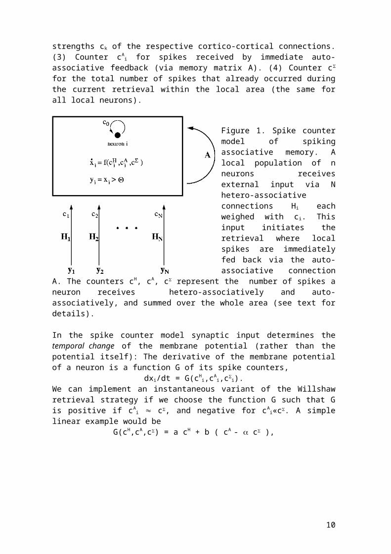
Figure 1 illustrates the basic structure of the spike counter model of associative memory as implemented for the MirrorBot project. A local population of n neurons constitutes a cortical area modelled as spiking associative memory using the spike counter model (Knoblauch and Palm 2001). Each neuron i has four states: (1) Membrane potential x . (2) Counter cH

i for spikes received hetero-associatively from N other cortical areas (memory matrices H1,…,HN) where in this model variant cH

i is not really a counter since the received spikes are weighed by connection strengths ck of the respective cortico-cortical connections. (3) Counter cA

i for spikes received by immediate auto-associative feedback (via memory matrix A). (4) Counter c for the total number of spikes that already occurred during the current retrieval within the local area (the same for all local neurons).

Figure 1. Spike counter model of spiking associative memory. A local population of n neurons receives external input via N hetero-associative connections Hi

each weighed with ci. This input initiates the retrieval where local spikes are immediately fed back via the auto-associative connection A. The counters cH, cA, c represent the number of spikes a neuron receives hetero-associatively and auto-associatively, and summed over the whole area (see text for details).

5

In the spike counter model synaptic input determines the temporal change of the membrane potential (rather than the potential itself): The derivative of the membrane potential of a neuron is a function G of its spike counters,

dxi/dt = G(cHi,cA

i,ci).

We can implement an instantaneous variant of the Willshaw retrieval strategy if we choose the function G such that G is positive if cA

i c, and negative for cAi«c. A simple

linear example would beG(cH,cA,c) = a cH + b ( cA - c ),

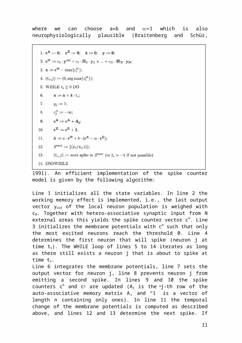
where we can choose a«b and 1 which is also neurophysiologically plausible (Braitenberg and Schüz, 1991). An efficient implementation of the spike counter model is given by the following algorithm:

Line 1 initializes all the state variables. In line 2 the working memory effect is implemented, i.e., the last output vector yold of the local neuron population is weighed with c0. Together with hetero-associative synaptic input from N external areas this yields the spike counter vector cH. Line 3 initializes the membrane potentials with cH such that only the most excited neurons reach the threshold 0. Line 4 determines the first neuron that will spike (neuron j at time ts). The WHILE loop of lines 5 to 14 iterates as long as there still exists a neuron j that is about to spike at time ts. Line 6 integrates the membrane potentials, line 7 sets the output vector for neuron j, line 8 prevents neuron j from emitting a second spike. In lines 9 and 10 the spike counters cA

and c are updated (Aj is the j-th row of the auto-associative memory matrix A, and “1” is a vector of length n containing only ones). In line 11 the temporal change of the membrane potentials is computed as described above, and lines 12 and 13 determine the next spike. If dx/dt is negative for all neurons no more spike will occur, and this will end the algorithm with the result y. A sequential implementation of this algorithm needs only O(n logn) steps (for n neurons and logarithmic pattern size) which is the same as for the classical Willshaw model. Parallel implementation requires O(log2 n) steps (only O(log n) for classical model).

6

2. Felix++: A tool for implementing cortical areas

The modules of work package 5 have been implemented using the Felix and Felix++ simulation tools. Originally the C based simulation tool Felix has been developed by Thomas Wennekers at the University of Ulm (Wennekers 1999) as a universal simulation environment for physical and in particular neural systems. The development of Felix was motivated by the need for fast implementation of multi-layer one- or two-dimensional neural structures such as neuron populations. For this purpose Felix provides elementary algorithms for single-cell dynamics, inter-layer connections, and learning. Additionally there exist also libraries for non-neural applications, e.g., for general dynamical systems and elementary image processing. Simulations can be observed and influenced online via the X11/XView-based graphical user interface (GUI) of Felix. The Felix GUI provides elements such as switches for conditional execution of code fragments, sliders for online-manipulation of simulation parameters (like connection strengths, time constants, etc.), and graphs for the online observation of the states of a simulated system in xy-plots or gray-scale images (Wennekers 1999; Knoblauch 2003_b, 2003_c). During the Mirrobot project the simulation tool Felix++ has been developed further as a C++ based object-oriented extension of Felix. Felix++ provides additionally classes for neuron models, n - dimensional connections, pattern generation, and data recording. Current installations of Felix++ are running on PC/Linux as well as on 64bit-SunFire/Solaris9 systems. In the following the architecture of Felix++ is briefly sketched (for more details see Knoblauch 2003_b, 2003_c).

2.1 Basic architecture of Felix++

Essentially Felix++ is a collection of C++ libraries supporting fast development of neural networks in C++ (Stroustrup 1997; Swan 1999). Thus Felix++ comprises a number of modules each consisting of a header (with the suffix ``.h'') and a corpus (with the suffix ``.cpp'' for Felix++/C++ or ''.c'' for Felix/C). The header files contain declarations of classes, types, and algorithms, whereas in the corpus files the declarations are implemented. Figure 2 illustrates the architecture of Felix++ by classifying all the modules of Felix++ and Felix in a hierarchy.

2.1.1 The core modules of Felix++

The core of Felix++ contains the most important modules required by all other Felix++ modules.

F2_types.h/cpp declares some elementary type conventions and some global objects.

F2_time.h/cpp declares classes for time, for example to evaluate the time necessary for computing a simulation.

F2_random.h/cpp provides several different random number generators (see Press et al. 1992).

F2_layout.h/cpp declares so-called layouts. A layout can be used to define the topology of a vector (or in terms of C++, an array). For example a population of 1000 neurons can be arranged as a 10 x 10 x 10 cuboid. Apart from cuboid layouts also ellipsoid layouts are defined which are useful in particular for saving memory when modeling isotropic local connectivity (in three dimensions, for

7

example, an ellipsoidal kernel saves almost 50 percent of the memory required by a cuboid kernel).

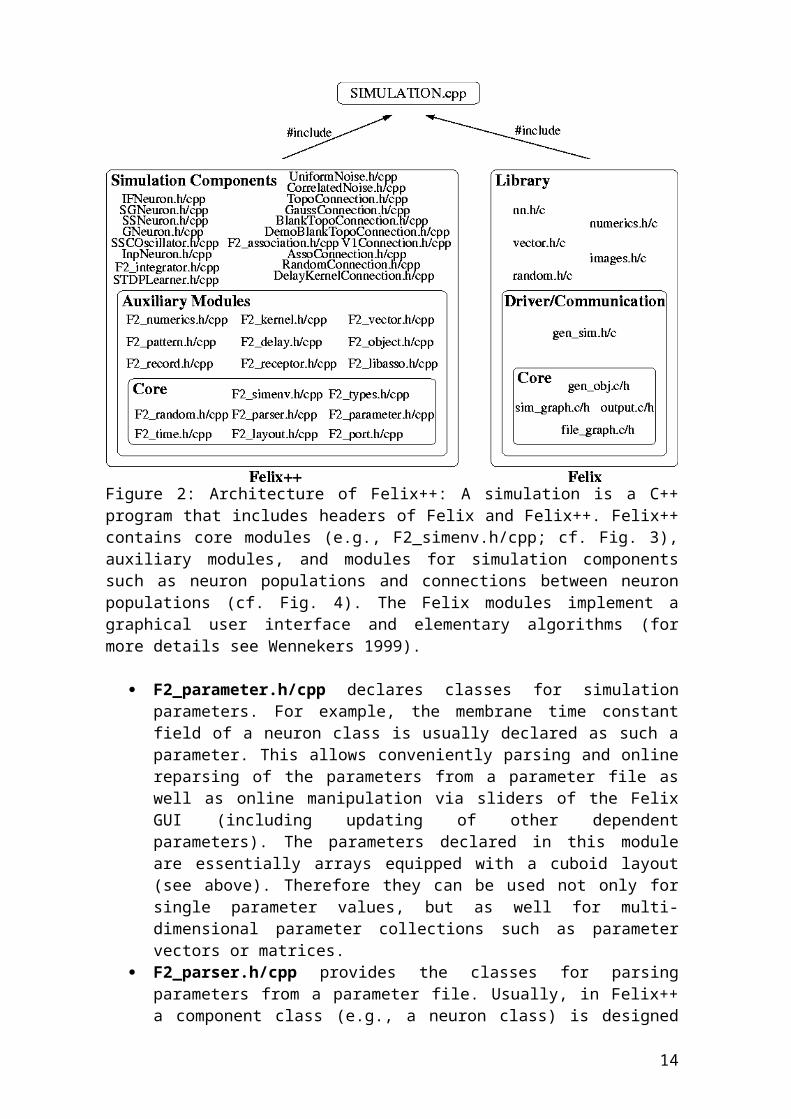
Figure 2: Architecture of Felix++: A simulation is a C++ program that includes headers of Felix and Felix++. Felix++ contains core modules (e.g., F2_simenv.h/cpp; cf. Fig. 3), auxiliary modules, and modules for simulation components such as neuron populations and connections between neuron populations (cf. Fig. 4). The Felix modules implement a graphical user interface and elementary algorithms (for more details see Wennekers 1999).

F2_parameter.h/cpp declares classes for simulation parameters. For example, the membrane time constant field of a neuron class is usually declared as such a parameter. This allows conveniently parsing and online reparsing of the parameters from a parameter file as well as online manipulation via sliders of the Felix GUI (including updating of other dependent parameters). The parameters declared in this module are essentially arrays equipped with a cuboid layout (see above). Therefore they can be used not only for single parameter values, but as well for multi-dimensional parameter collections such as parameter vectors or matrices.

F2_parser.h/cpp provides the classes for parsing parameters from a parameter file. Usually, in Felix++ a component class (e.g., a neuron class) is designed in such a way that a construction of an object is paralleled by parsing the corresponding parameters from a file. Furthermore, during the simulation the parameter file can be modified and reparsed by pressing the reparse-button.

F2_port.h/cpp declares interfaces for the communication between different simulation components, so-called ports. For example, a neuron class may contain an output port representing the spikes of the neuron, and an input port representing synaptic input to the neuron. Correspondingly, the constructor of a connection component class requires as parameters the output port of a neuron population and the input port of another neuron population such that the spikes

8

from the first population can be propagated to the dendrites of the second population.

F2_simenv.h/cpp declares the simulation environment class TSimulationEnvironment and the component base class TComponent as well as some base classes for special components such as neurons (TNeuron) and connections (TConnection). This module should be included by any simulation program using Felix++. The simulation environment is essentially a container for the simulation components (see below for more details; cf. Fig. 3, but provides also additional infrastructure such as look-up tables (for example for Gaussians), random number generators, and much more. Usually, the construction of a simulation component requires a TSimulationEnvironment as an argument, such that the component is automatically inserted. After construction of all the components, calls to methods allocate() will allocate memory shared by multiple components (for example when integrating differential equations via TIntegrator objects; see below). Before starting the simulation all the components can be initialized by calling the init() method of the simulation environment. And similarly, during the simulation a call to the step() method will compute one simulation step.

Figure 3. The simulation environment object (of class TSimulationEnvironment) is essentially a container object containing all the simulation components such as neuron populations or connections. The components are inserted during construction. Before starting a simulation a call to method allocate() is necessary to allocate memory. A call to init() initializes the components, and each call to step() results in the computation of one simulation step.

2.1.2 Auxiliary modules of Felix++

Besides the core modules there is a number of auxiliary modules that provide additional functionality required by only some of the Felix++ component modules, but perhaps also by the programmer developing a simulation.

F2_numerics.h/cpp provides a number of useful constants (e.g., , e, and ln 2) and functions (e.g., density function of Binomials or Gaussians, information and transinformation functions for binary random variables, etc.). Further declarations provide classes for look-up-tables and interpolation.

F2_kernel.h/cpp declares classes for kernels that can be used, for example, for implementing synaptic connections. Kernels are essentially arrays (e.g., of synaptic weights or delays) that have been assigned a topology via layouts (see F2_layout.h/cpp). The classes defined in this module enable, for example, the

9

coordination of a neuron population (layout) to a set of kernels. This happens in a rather flexible manner such that each neuron can be assigned individually a kernel index, where also certain regularities of kernel arrangements can be exploited.

F2_vector.h/cpp provides basic vector functionality. This module also declares classes for numerical vector parameters (cf. F2_parameter.h/cpp).

F2_pattern.h/cpp implements classes for various types of patterns. From the pattern base type (TMPattern) which corresponds simply to a multi-dimensional array there are derived specialized pattern types such as binary patterns (TMbPattern), sparse binary patterns (TMsbPattern), sparse patterns (TMsPattern), or sparse binary spatio-temporal patterns (TMsbSTPattern). Additionally further auxiliary classes have been implemented in order to facilitate the use of patterns. For example, pattern container classes are declared (TMPatternStock and derivatives of TMPatternGroup) for convenient construction and parsing of pattern groups from parameter files. The TMPatternRanking class can be used for analyzing neural activity with respect to a set of pattern (i.e., to determine the pattern in the set that is most similar to the neural activity pattern). Similarly the TMPatternHistogram class can be used to create pattern-specific histograms of state variables.

F2_delay.h/cpp provides classes based on the definitions in F2_kernel.h/cpp for efficient implementation of synaptic delays.

F2_object.h/cpp declares classes for generating stimulus objects. Further classes can be used to put static or moving objects in space (derivatives of TMSpace), or projecting the stimulus configuration onto a two-dimensional surface (derivatives of TMSpaceRepresentation).

F2_record.h/cpp provides the infrastructure for efficient recording of simulation data.

F2_receptor.h/cpp declares classes for the efficient implementation of various types of receptors for synaptic transmitters. Derivatives of class TMReceptorPort can be used, for example, to implement certain transmitter-dependent synaptic conductances (e.g. for AMPA, GABA-A, GABA-B, NMDA receptors). Actually neuron classes such as TSSNeuron or TGNeuron use the receptor port classes provided by this module. These models can be equipped with an arbitrary configuration of different receptor ports which can be specified in the parameter file (see below).

F2_libasso.h/cpp} encapsulates the C-library for associative memory implemented by Friedrich Sommer (Sommer and Palm, 1999).

2.1.2 Component classes of Felix++

Based on the core and auxiliary modules there exists already a large number of simulation components. Figure 4 illustrates the class hierarchy of the Felix++ simulation components. They can be divided into the following component base classes derived from TComponent:TNeuron (defined in module F2_simenv.h/cpp) is the base class for all neuron classes. Currently there are implementations for gradual neurons (TSGNeuron in module SGNeuron.h/cpp and TGNeuron in module GNeuron.h/cpp), spiking neurons (TIFNeuron in module IFNeuron.h/cpp and TSSNeuron in module SSNeuron.h/cpp), and oscillators (TSSCOscillator in module SSCOscillator.h/cpp) which all can be used for biological modeling. Additionally there are classes adequate for technical implementations of associative memory e.g., classes TMAssociationPopulation and TMAutoWillshawTAMP

10

in module F2_association.h/cpp. The latter class has been used for the implementation of Willshaw associative memory and the spike counter model for the language areas.

Figure 4. The class hierarchy for the currently implemented simulation components of Felix++. From the base class TComponent specialized sub-classes are derived for neuron populations (TNeuron), noise generators (TMNoise), connections between neuron populations (TConnection), integration of differential equations (TMIntegrator), synaptic plasticity (TLearner), representations of stimulus space (TMSpace), and on-line observation of the simulation state (TObserver).

TMNoise (defined in module F2_simenv.h/cpp) is the base class for noise populations. A noise population provides random numbers generated according to a certain distribution for another component object such as a neuron population. Derivations of type TMUniformNoise (defined in module UniformNoise.h/cpp) provide uniformly distributed random numbers with a certain power (or variance). While this type generates independent random numbers in each simulation step the random numbers generated by derivations of type TMCorrelatedNoise can be correlated in space and time. The standard noise type for neuron populations such as TSSNeuron (or for synaptic noise in connections; see module F2_receptor.h/cpp) is TMUniformNoise.

TConnection (defined in module F2_simenv.h/cpp) is the base class for connections between neuron populations (or more exactly, between ports; see module F2_port.h/cpp). The function of derivations from this type is to propagate information from an output port to an input port, for example, to propagate the spikes from the output port of one neuron population through the network to the input port of another neuron population. The most important derived type for biological modeling is TMTopoConnection (defined in module TopoConnection.h/cpp). This generic type is the base class for many further derived classes. Here a synapse is defined by two state values: a synaptic weight, and a synaptic delay. Correspondingly, an object of type TMTopoConnection essentially contains two kernel arrays of type TKernel (defined in F2_kernel.h/cpp) representing weights and delays. The kernel classes can be applied in a very flexible manner allowing implementation of full, sparse, topographical schemes in multiple dimensions. Additionally, efficient algorithms are implemented for several special cases (e.g., for non-sparse bit-packed binary topographical connectivity). The derivatives of TMTopoConnection merely specify how the synaptic weight and delay kernels are generated. For example, class TMGaussConnection (defined in module GaussConnection.h/cpp)

11

implements simple topographical connections with Gaussian kernels. A further derived class TMBlankTopoConnection (defined in module BlankTopoConnection.h/cpp) provides an interface to TMTopoConnection in order to allow a more convenient derivation of further connection classes. While TMDemoBlankTopoConnection (defined in DemoBlankTopoConnection.h/cpp) is merely a demonstration how to derive from TMBlankTopoConnection, also a number of important connection classes have been derived. TMAssoConnection (defined in module AssoConnection.h/cpp) can be used to implement fully connected or multi-dimensional topographically confined associative connections, for example, of the Willshaw type. TMV1Connection (defined in module V1Connection.h/cpp) is a specialized connection scheme for the primary visual cortex. And TMRandomConnection (defined in RandomConnection.h/cpp) can be used conveniently for implementing connections with random connectivity. Another class derived directly from TConnection is TMDelayKernelConnection (defined in module DelayKernelConnection.h/cpp) which provides a much simpler and faster scheme for delayed connections than TMTopoConnection. For implementation of technical associative memory derivations from class TMAssociation (defined in module F2_association.h/cpp) can be used, such as TMWillshawAssociation and TMcWillshawAssociation for the Willshaw model, where the latter implements compression of the binary memory matrix.

TMIntegrator (defined in module F2_integrator.h/cpp) is the base class for numerical integration of differential equations. Derived classes (defined in the same module) are TMEulerIntegrator which implements a simple first order Euler method, and TMRK4cIntegrator which implements the fourth order Runge-Kutta method with constant step size (see Press et al. 1992). Normally, these integrator objects are used by some of the neuron classes (e.g., TSSNeuron).

TLearner (defined in module F2_simenv.h/cpp) is the base class for plasticity of synaptic connections. Currently, two derivatives are implemented in the module STDPLearner.h/cpp. TMSTDPLearnerSMA2000 implements a model of spike-timing dependent synaptic plasticity (STDP) described by Song, Miller, and Abbott (2000), while TMSTDPLearnerFD2002 implements an extended model suggested by Froemke and Dan (2002). Both classes are interfaced with connection classes via the kernel classes defined in F2_kernel.h/cpp. Therefore it is easy to endow connections (e.g., derived from TMTopoConnection) with synaptic plasticity.

TMSpace (defined in module F2_object.h/cpp) is the base class for the definition of a space for stimulus objects (see above module F2_object.h/cpp).

TObserver (defined in module F2_simenv.h/cpp) is the base class for components observing on-line the state of the simulation. Derived classes are TMPatternRanking and TMPatternHistogram (for more details see above module F2_pattern.h/cpp).

2.2 Structure of a Felix++ simulation

2.2.1 A skeleton simulation program

A Felix++ simulation is basically a C++ program that includes header files of Felix and/or Felix++. The structure of a Felix++ simulation typically looks similar to the following code fragment:

12

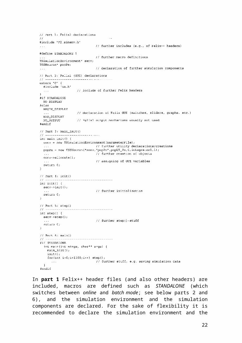
In part 1 Felix++ header files (and also other headers) are included, macros are defined such as STANDALONE (which switches between online and batch mode; see below parts 2 and 6), and the simulation environment and the simulation components are declared. For the sake of flexibility it is recommended to declare the simulation environment and the components as pointer variables which are allocated in the main_init() method (see part 3). For example, if the simulation environment and components would be already constructed here, it would be not possible to pass the name of the parameter file to be

13

used as an argument to the simulation program. In this example only the simulation environment senv and a neuron population popPe of type TSSNeuron (see above) are declared. Usually the construction of the simulation environment and the simulation components is paralleled with the parsing of a parameter file (see below). In part 2 the graphical user interface (GUI) of the simulation is declared (only necessary for online simulations, i.e., if the flag macro STANDALONE is inactive). For this purpose, first the Felix headers (see Fig. 2) must be included (in extern ``C'' brackets since Felix has been implemented in C). Then the GUI components of Felix can be specified in the #else branch of the #if directive (for details see Wennekers, 1999).Part 3 is the main_init() procedure. Here the simulation environment and subsequently the simulation components are created by calling the corresponding constructors. After constructing all simulation components, a call to the allocate() method of the simulation environment might be necessary (e.g., for simulation components such as TSSNeuron employing integrators; see above module F2_integrator.h/cpp). The main_init() procedure is normally called only once at the beginning of the simulation to construct the simulation objects. This is done either by the main() procedure (see part 6) for batch simulations (for activated flag macro STANDALONE=1) or by the Felix GUI for online simulations (for STANDALONE=0).In part 4 the init() procedure is defined. It contains normally at least the call to the init() method of the simulation environment, but possibly also further initialization code for the simulation. The init() procedure should be called after main_init() to initialize the states of the simulation objects before the actual simulation computations start (see part 5). In contrast to main_init() the init() procedure can be called more than once either from the main() procedure (see part 6) for batch simulations or for online simulations by pressing the init button (or the run button) in the main simulation window (Wennekers 1999).Part 5 is the step() procedure which computes one simulation step. It contains normally at least the call to the step() method of the simulation environment, but possibly also further code for the simulation. The step() procedure is called either from the main() procedure (see part 6) for batch simulations or for online simulations by pressing the step button (or the run button) in the main simulation window.Part 6 defines the main() procedure for batch simulations with activated macro flag STANDALONE=1 (see part 1). This procedure must contain calls to main_init() and init() before the calls to the step() procedure.

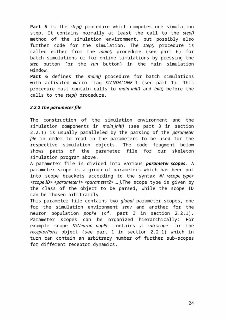
2.2.2 The parameter file

The construction of the simulation environment and the simulation components in main_init() (see part 3 in section 2.2.1) is usually paralleled by the parsing of the parameter file in order to read in the parameters to be used for the respective simulation objects. The code fragment below shows parts of the parameter file for our skeleton simulation program above.A parameter file is divided into various parameter scopes. A parameter scope is a group of parameters which has been put into scope brackets according to the syntax #{ <scope type> <scope ID> <parameter1> <parameter2> ... }.The scope type is given by the class of the object to be parsed, while the scope ID can be chosen arbitrarily.This parameter file contains two global parameter scopes, one for the simulation environment senv and another for the neuron population popPe (cf. part 3 in section 2.2.1). Parameter scopes can be organized hierarchically: For example scope SSNeuron popPe contains a sub-scope for the receptorPorts object (see part 1 in section 2.2.1) which in turn can contain an arbitrary number of further sub-scopes for different receptor dynamics.

14

In the example there are two scopes for the receptor dynamics (cf. module F2_receptor.h/cpp) specifying the dynamics of the synaptic conductances of the neuron model. The parameters in scope TMOffDynamicsRP AMPA specify the dynamics of an AMPA-like excitatory conductance which is implemented by a corresponding object of type TMOffDynamicsRP. Parameter tau_OFF corresponds to the conductance decay time constant, i.e., the conductance decays exponentially following an instantaneous increase caused by an incoming spike. Parameter E corresponds to the equilibrium (or reversal) potential. The additional parameters determine conductance offset (g0), noise power (powerInpNoise), and the queue length (qLen; measured in simulation steps) for incoming spikes propagated by connection objects (see above class TConnection). The latter parameter determines the maximal possible axonal delay for the connection projecting onto this receptor port.The parameters in scope TMOffDynamicsRP GABAA have the analogous relation to GABA-like dynamics of an inhibitory conductance.Many parameters are specified not by a single value but by a vector of four values to individual parameters for each member of a population. Parameter refRel (in scope popPe), for example, specifies that the parameter for relative refractoriness of the neuron model TSSNeuron is distributed according to a Gaussian with mean 3, standard deviation 0.5, but limited to the interval [1.75; 4.25]. In contrast, if the standard deviation is 0 and/or the left interval border larger than the right one then the parameter is the same for all members of the population (see parameter tau_x, for example).

2.2.3 Compiling and running simulations

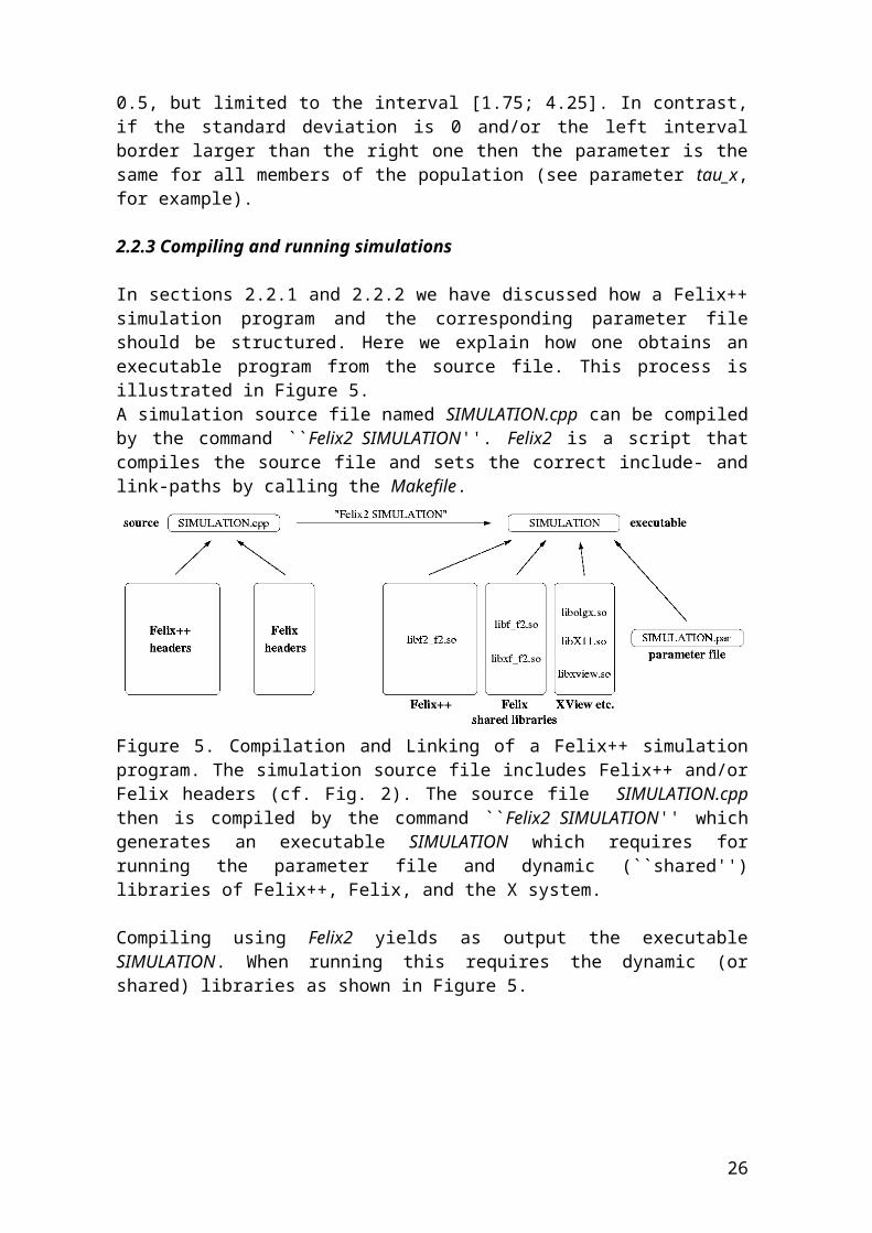
In sections 2.2.1 and 2.2.2 we have discussed how a Felix++ simulation program and the corresponding parameter file should be structured. Here we explain how one obtains an executable program from the source file. This process is illustrated in Figure 5. A simulation source file named SIMULATION.cpp can be compiled by the command ``Felix2 SIMULATION''. Felix2 is a script that compiles the source file and sets the correct include- and link-paths by calling the Makefile.

15

Figure 5. Compilation and Linking of a Felix++ simulation program. The simulation source file includes Felix++ and/or Felix headers (cf. Fig. 2). The source file SIMULATION.cpp then is compiled by the command ``Felix2 SIMULATION'' which generates an executable SIMULATION which requires for running the parameter file and dynamic (``shared'') libraries of Felix++, Felix, and the X system.

Compiling using Felix2 yields as output the executable SIMULATION. When running this requires the dynamic (or shared) libraries as shown in Figure 5.

16

3. Implementation of cortical language areas

3.1 Model of cortical language areas

Figure 6 shows the 15 areas of our model for cortical language processing. Each of the areas is modeled as a spiking associative memory of 100 neurons (see section 1). For each area we defined a priori a set of binary patterns (i.e., subsets of the neurons) constituting the neural assemblies. These patterns were stored auto-associatively in the local synaptic connectivity according to a simple Hebbian learning rule (cf. section 3.2 in report 5). In addition to the local synaptic connections we also modelled extensive inter-areal hetero- associative connections between the cortical areas (see Fig. 6).

Figure 6. Cortical areas and inter-areal connections. Each of the 15 areas was implemented as a spiking associative memory (size 100 neurons) including auto-associative synaptic connections as described in section 1. Each black arrow corresponds to a hetero-associative synaptic connection that associates specifically corresponding assemblies of the involved presynaptic and postsynaptic cortical areas by Hebbian learning. Together with the local auto-associative synaptic feedback constitute the long-term memory of the model. In contrast, the blue feedback arrows indicate the areas implementing a short-term memory mechanism. The model can roughly be divided into three parts. (1) Primary cortical auditory areas A1,A2, and A3: First auditory input is represented in area A1 by primary linguistic features (such as phonemes), and subsequently classified with respect to function (area A2) and content (area A3). (2) Grammatical areas A4, A5-S, A5-O1-a, A5-O1, A5-O2-a, and A5-O2: Area A4 contains information about previously learned sentence structures, for example that a sentence starts with the subject followed by a predicate. The other areas contain representations of the different sentence constituents (such as subject, predicate, or object, see below for details). (4) Activation fields af-A4, af-A5-S, af-A5-O1, and af-A5-O2: The activation fields are relatively primitive areas that are

17

connected to the corresponding grammar areas. They serve to activate or deactivate the grammar areas in a rather unspecific way.We stress that the area names we have chosen should not be interpreted as the names of cortical areas of the real brain used by neurophysiologists. However, we suggest that areas A1,A2,A3 might be interpreted as parts of Wernicke’s area, and area A4 as a part of Broca’s area. The complex of the grammatical role areas A5 might be interpreted as parts of Broca’s or Wernicke’s area. The activation fields can be interpreted as thalamic nuclei.

3.2 Neural assemblies of the language areas

Each area consists of spiking neurons that are connected by local synaptic feedback. Previously learned word features, whole words, or sentence structures are represented by neural assemblies (subgroups of neurons, i.e., binary pattern vectors), and laid down as long-term memory in the local synaptic connectivity according to Hebbian coincidence learning (Hebb 1949). In our implementation we used the Willshaw model of associative memory for binary patterns and binary synapses. Previously learned entities are represented by neural assemblies of 5 out of 100 neurons (i.e., the patterns are binary vectors of length 100 that contain 5 ones and 95 zeros). Overlaps of different patterns can be used to express similarities between the represented entities.In the following we describe the function and the neural assemblies of the individual areas (see Fig. 6) in more detail:

Area A1 is a primary auditory cortical area which receives preprocessed acoustic input. Currently we have defined one neural assembly for each entity that can occur in the MirrorBot scenarios. In future we plan to implement a more general coding scheme where acoustic input is represented by elementary linguistic features such as phonemes (cf. Fromkin and Rodman 1974).

Area A2 contains neural assemblies _start, _end, _blank, and _word. This area classifies the representations in area A1. For example, if area A1 contains phonetically the representation of a known word this will activate the assembly _word in area A2. If area A1 represents the transition from one word to the next then this would activate the _blank-assembly. And if the beginning or ending of a sentence is detected this is represented by the _start and _end assemblies, respectively.

Area A3 contains one assembly for each word that can occur in the MirrorBot scenarios (see report 2). Currently the assemblies are designed such that similiarities between the represented entities are reflected in the overlaps between the different assemblies. Alternatively, the assemblies could also reflect similarities between the linguistic (e.g., phonetic) representations of the entities, i.e., word form rather than word content. Moreover, we have the idea that in the global model area A3 would be reciprocally connected with various non-language areas representing other (e.g., visual, motor, etc.) semantic aspects of the entities.

The grammatical sequence area A4 currently contains assemblies sntnc_S, sntnc_P, sntnc_vp1_O1, sntnc_vp2_O1, sntnc_vp2_O2, and sntnc_end representing the grammatical constituents of a sentence like subject, predicate and object. In order to represent grammatically correct sentence structures the elementary assemblies are connected to sequences. Currently we have stored the sequences (S,P,vp1_O1) and (S,P,vp2_O1,vp2_O2) according to two verb patterns. For example verb pattern vp1 represents verbs expecting only one object (as for the verb “show” in the sentence “Bot show plum”), and similarly vp2 represents verbs expecting two objects (as for the verb “put” in the sentence “Bot

18

put apple (to) plum!”). Information about the valid sequences is stored in a delayed hetero-associative synaptic feedback connection within area A4. For example, for the sequence (S, P, vp1_O1, _end) we have to store the associations (S, P), (P, vp1_O1), and (vp1_O1, _end). See report 5 for further details.

Area A5-S contains assemblies representing the known entities that can be the subject of a sentence. Currently we have only two possible subjects, namely bot, and sam representing the robot and its instructor, respectively.

Area A5-P contains assemblies stop, go, move_body, turn_body, turn_head, show, pick, lift, drop, touch, and put, representing the possible predicates of current MirrorBot sentences.

Areas A5-O1 and A5-O2 contain assemblies representing the possible objects of sentences. Currently these are nut, plum, dog, cat, desk, wall, ball, cup, apple, forward, backward, left, right, up, and down.

Areas A5-O1-a and A5-O2-a contain assemblies representing object attributes. Currently these are brown, blue, black, white, green, and red.

Additionally, areas A3, A5-S, A5-P, A5-O1, A5-O1-a, A5-O2, and A5-O2-a also contain an assembly _none to represent unknown or inappropriate entities.

The activation fields af-A4, af-A5-S, af-A5-P, af-A5-O1, and af-A5-O2 are rather primitive areas that contain only two or three assemblies activate, deactivate, and sometimes deactPart. The activation fields serve to rather unspecifically activate or deactivate the corresponding cortical area. Therefore we have the idea that the activation fields can be interpreted as some sub-cortical (for example thalamic) locations rather than cortical areas.

When processing a sentence then the most important information stream flows from the primary auditory areas A1 via A3 to the grammatical role areas A5-S, A5-P, A5-O1, A5-O1-a, A5-O2, and A5-O2-a. From there other parts of the global model can use the grammatical information to perform, for example, action planning. The routing of information from area A3 to the grammatical role areas is guided by the grammatical sequence area A4 which receives input mainly via the primary auditory areas A1 and A2. This guiding mechanism of area A4 works by activating the respective grammatical role areas appropriately via the activation fields af-A5-S, af-A5-P, af-A5-O1, and af-A5-O2. In section 4 (see also section 4 in report 5) we will further illustrate the interplay of the different areas when testing the model. In the following we will describe the implementation of the model using the Felix++ simulation tool.

3.3 Implementation using Felix++

The current implementation of the language areas comprises the following files: ./demo/lang3_qt.cpp: The core simulation program containing the Felix++

simulation objects and the procedures main_init(), init(), and step() (see section 2.2.1).

./demo/lang3_qtDemo.par_MirrorBot: The parameter file for the simulation program ./demo/lang3_qt.cpp (see section 2.2.2).

./demo/lang_qtDemo.h/cpp: Interface between the core simulation and QT. Delivers classes for online-visualization of the simulation in QT beyond the XView-based standard visualization of Felix/Felix++ (cf. section 2).

./demo/DrawWidget.h/cpp: Defines widgets extending QT’s QWidget for visualization of the language areas (cf. Figs. 7-9).

./demo/onlineinput.cpp: Defines classes for online-processing of acoustic input which can be generated either by the MirrorBot voice recognition software or by

19

the GUI classes defined in ./dialog/dialog.h/cpp. Currently only the latter programs are interfaced with the simulation program.

./demo/main.cpp: Contains the main() procedure of the simulation program. ./demo/Makefile: “make all” will compile all files in the ./demo/ directory. ./dialog/dialog.h/cpp: Defines classes for generating acoustic input for the

language areas via a QT graphical user interface. It delivers one button for each word in the MirrorBot grammar (see report 2).

./dialog/main.cpp: Contains the main() procedure of the dialog program for generating acoustic input.

./dialog/Makefile: “make all” will compile all files in the ./dialog/ directory.Compiling requires calling the two Makefiles (“make all”) in the ./demo/ and ./dialog/ directories. Subsequently the simulation can be started by calling the two executables “./demo/demo&” and “./dialog/dialog&”.In the following we will give a more detailed description of the core simulation program, lang3_qt.cpp.

3.4 The core simulation program

The core simulation program lang3_qt.cpp implements the model described in sections 3.1 and 3.2 (see also report 5) using the Felix++ simulation tool (see section 2). The following code fragment declares the simulation components (corresponding to part 1 of the skeleton simulation shown in section 2.2.1).

For the neuron populations (corresponding to the area boxes in Fig. 6) we use the Felix++ class TMAutoWillshawTAMP (module F2_association.h/cpp; see section 2.1.2; see Fig. 4) for technical associative memory which also implements the spike counter

20

algorithm (see section 1.1). For each cortical area and each activation field a TMAutoWillshawTAMP object is declared (e.g. popA1 for area A1, and afA4 for activation field af-A4).In order to control the network performance we explicitely represent the stored assemblies or patterns (while they are also represented implicitely in the synaptic connections, of course) using the Felix++ container class TMPatternStock of module F2_pattern.h/cpp (see section 2.1.2). For example, patA5P contains all patterns representing the verbs in area A5-P (see section 3.2). To be able to decide during the simulation which pattern is most similar to the current neural activation pattern of a given neuron population we use the Felix++ class TMPatternRanking (module F2_pattern.h/cpp; see section 2.1.2) which can compute online rankings for the minimal hamming distance or the maximal transinformation, for example.For connections between the cortical areas and activation fields we use the Felix++ connection class TMAssoConnection (module AssoConnection.h/cpp; see Fig.4; see section 2.1.2). For example, object link_A3_A5P is the hetero-associative connection from area A3 to area A5-P. The long-term memory corresponding to these connections can be specified in the parameter file (see below) using the Felix++ matrix parameters TsMatPar (module F2_parameter.h/cpp; see section 2.1.1). For example, projDef_A3_A5P specifies which assemblies of area A3 are connected to which assemblies in area A5-P.The code fragment shown below contains parts of the main_init() procedure of lang3_qt.cpp (corresponding to part 2 of the skeleton simulation in section 2.2.1).

21

Here the simulation components are allocated by calling the corresponding constructors of the Felix++ classes and thereby parsing the corresponding parameter file. First the neuron populations for each area is constructed by calling the constructor of class TMAutoWillshawTAMP. The first call for population popA1 parses scope AutoWillshawTAMP pops in parameter file lang3_qtDemo.par_MirrorBot (see section 2.2.2) which is shown below:

Here essentially the parameters of the spike counter algorithm (see section 1.1) are specified. The following constructor calls (e.g, for popA2 and popA3) use popA1 as argument and thereby use the same parameters as specified for popA1. In the next part of the main_init() procedure the assemblies or patterns are defined. For example, patA5P is allocated by calling the constructor of class TMPatternStock. This allocates the object using the parameters of scope PatternStock patA5P from the parameter file as shown below:

Here the verb assemblies constituting the long-term memory of area A5-P are specified as binary patterns (of length 100) containing 5 one-entries in the first pattern group (of type TMParsedPG defined in Felix++ module F2_pattern.h/cpp; see section 2.1.2). For example the assembly representing the verb “put” is represented by the neurons with the indices 20, 21, 54, 55, and 56. The second pattern group defines a pattern containing all the neurons of area A5-P (for unspecific thalamic input). And the third pattern group defines additional patterns corresponding to the three verb patterns of the MirrorBot grammar. Note that the latter patterns are parts of the individual verb assemblies in the first pattern group, and thereby are used to express (grammatical) similarity.Next in the main_init() procedure the object projDef of type TMParameterGroup is constructed which is used for parsing the matrix parameters of type TsMatPar. (defined

22

in Felix++ module F2_parameter.h/cpp; see section 2.1.1). The next code fragment shows the matrix parameters projDef_A3_A5P and projDef_A4_A4 as specified in the parameter file.

For example, projDef_A3_A5P specifies that the word assemblies in area A3 are connected to the corresponding assemblies in area A5-P (e.g., assembly show in A3 is connected to assembly show in A5-P). Similarly, parameter projDef_A4_A4 specifies the delayed auto-associative connection of area A4 which defines the grammatical sequences (see sections 3.1 and 3.2; cf. section 3.2 in report 5). For example, the association from assembly sntnc_S to assembly sntnc_P specifies that the predicate follows the subject (cf. Fig. 6 in report 5).

3.5 The visualization

In order to visualize the neural activity in the model of cortical language areas online during the simulation we have designed three graphical windows using the QT library

(see module DrawWidget.h/cpp in directory ./demo/; see section 3.3). Figure 7 shows the first visualization: Here we have embedded the model into an image of a brain. It is also the main control window of the simulation. On the bottom there is a row of different buttons. The reparse, init, step, and run buttons correspond to the Felix/Felix++ GUI (see section 2). The saveImg button can be used for saving the contents of the three visualization windows. And the areas and output buttons are used for opening and closing the remaining visualization windows.

Figure 7: The brain-embedded model visualization.

23

The second visualization is shown Figure 8. Here the areas are drawn similar as in Figure 6 (and in the figures of report 5).

Figure 8: Visualization of the cortical and subcortical language areas of the model. Compare to Fig. 6. See text for details.

Each box corresponds to a cortical or subcortical language area. In the left upper corner of the box the area name is written (e.g. A1). In the upper right corner the number of active (i.e. spiking) neurons is indicated. For example, (#: 5/100) means that 5 neurons of a total of 100 neurons are currently active. The bold-type characters on the central white field indicate the name of the activated assembly, for example plum in area A1. If no assembly is active this is indicated by _null. On the bottom line two quality measures are printed. For example, for area A1 the text t/c 1.00/1.00 means that the transinformation between the stored assembly plum and the current neural activation pattern is t=1.00 and also the completeness of the assembly is perfect (c=1.00). The text in the upper left corner of the window indicates that the currently processed acoustic input is “plum”. And the text in the upper right corner of the window indicates that the last computed simulation step was step 81.The third visualization is hown in Figure 9. Here essentially the same information as in Figure 8 is given, but only the output areas relevant for the result of the grammatical analysis are shown.

Figure 9: The output visualization shows only the cortical areas representing the result of the grammatical analysis.

24

3.6 Integration with other MirrorBot components

The described implementation of the model of cortical language areas can be easily integrated with other MirrorBot components using the CORBA based MIRO-framework (see Utz et al. 2002; cf. Enderle et al. 2003). When integrating other components will use the grammatical analysis performed by the described model, for example, to execute spoken commands to the robot (cf. Fig. 9; cf. Wermter et al. 2003; cf. also Weber and Wermter 2003; Frezza-Buet and Alexandre, 2002). Exemplarily we have implemented a simple graphical input window for generating acoustic input for our model illustrated in Figure 10 (see ./dialog/dialog.h/cpp module described in section 3.3).

Figure 10: Dialog window for generating acoustic input for the language model.

Herewith we can simulate a microphone and the subsequent speech recognition module. For switching on the microphone the Micro on button has to be pressed. Then a sentence corresponding to the MirrorBot grammar (see report 2) can be generated by pressing the appropriate word buttons. Pressing the Micro on button for a second time will switch off the microphone.The simulation program of the cortical language areas and the dialog component for generation of acoustic inputs are two processes and run independently of each other, where the two processes communicate via an commonly used file. Currently the data format is word-based assuming that the speech recognition module recognizes correctly the words (but we also we could use word features such as phonemes). On the output side our model produces a grammatical segmentation of a sentence which can easily be used by other modules of the MirrorBot project (either by explicitely delivering the symbolic information about word and grammatical role, or by directly using the respective assembly code). In the next section we illustrate some tests performed with our model of cortical assemblies of language areas.

25

4. Test of the model

In this section we test the implementation of our model of cortical language areas (see section 3). We do this by using the ./dialog/dialog program to generate acoustic input (see sections 3.3 and 3.6). First we demonstrate that the model is capable of processing and interpreting correctly sentences that are correct with respect to the MirrorBot grammar definition (see report 2). Then we test what happens for sentences that are not correct with respect to the grammar definitions.

4.1 Processing of a correct sentence

We repeat the test described in report 5 (section 4) with our current implementation of cortical language areas. During processing of acoustic input we show the area visualization (see Fig. 8) for some particular simulation steps .For this test the acoustic input was

“MicOn bot put plum green apple MicOff”.The small letters MicOn and MicOff corresponds to the microphone being switched on or off (cf. section 3.6) which cause _start and _end events. Similarly a word border causes a _blank event (cf. section 4 in report 5).The following figure shows the network state after simulation step 6. Initially the activation fields are in the deactivating state except for area A4. The processing of a

sentence beginning activates the _start assembly in area A2 which activates sntnc_S in A4 which activates af-A5-S which primes A5-S. When subsequently the word “bot” is processed in area A1 this will activate the _word assembly in area A2, and the bot assemblies in area

A3 and area A5-S. The next snapshot illustrates the network state after step 16. The _blank representing the word border between words “bot” and “put” is recognized in area A2 which activates the _deactivate assembly in af-A4 which deactivates area A4 for one simulation step. Immediately after the _blank the word “put” is processed

26

in A1 which actives the _word and put assemblies in areas A2 and A3, respectively. This will activate again area A4 via af-A4. Due to the delayed intra-areal feedback this will activate the sntnc_P representation in area A4 as the next sequence assembly. This activates the activate assembly in af-A5-P which primes A5-P to be activated by the put representation in area A3. The next snapshot is after step 24. The word border between the words “put” and “plum” activates the _blank assemblies in areas A1 and A2 which activates the _deactivate representation in activation field af-A4 which temporarily deactivates area A4. When the

plum pattern enters area A1 this activates the _word representation in area A2 which results in activating again the _activate assembly in activation field af-A4. This reactivates area A4 where the delayed auto-associative feedback within area A4 as well as synaptic

input from area A5-P activates the sequence assembly sntnc_vp2_O1 in area A4. This will activate activation field af-A5-O2 and prime areas A5-O1-a and A5-O1. At the same time the plum representation is activated in area A3 and routed further to the primed area A5-O1. Since in area A5-O1-a no representation corresponding to plum exists, here the _none assembly is activated.The next snapshot is after step 32. The word border between “plum” and “green” activates the _blank representations in area A1 and A2 which initiates the switching of

the sequence assembly in area A4 to its next part as described before. The activation of the part sntnc_vp2_O2 activates the _activate assembly in activation field af-A5-O2 which primes areas A5-O2-a and A5-O2. Then the processing of the word “green” activates the ‘green’

assembly in area A5-O2-a via areas A1 and A3. Since there exists no corresponding representation in area A5-O2 here the _none assembly is activated. The next snapshot is after step 39 where the processing of the sentence is almost complete. When the word border between “green” and “apple” is processed we have still the _none assembly activated in area A5-O2 (see above). This prevents the activation of the _deactivate assembly in activation field af-A4 and therefore also the switching in area

27

A4 from the sequence part sntnc_vp2_O2 to _end. Further together with the word border representation _blank in area A2 the _none assembly in area A5-O2 activates the _deactPart assembly in af-A5-O2 which deactivates area A5-O2. As soon as the

word “apple” is processed and represented by the _word and apple assemblies in areas A2 and A3, respectively, the activate assembly is again activated in activation field af-A5-O2. This primes again area A5-O2, and therefore the apple representation can be activated via input from area A3. Finally in the last snapshot showing the simulation state after step 46 the next word

border (or more exactly: the end of the sentence) will switch the sequence assembly in area A4 to its final part _end. This indicates that the processed sentence was actually correct. While areas A1, A2, and A3 return to the resting state without any activity, the

assemblies in areas A5-S, A5-P, A5-O1-a, A5-O1, A5-O2-a, and A5-O2 remain active due to the short-term memory mechanism (see Fig.6). Thus this activity constitutes the result and can be used by other cortical areas, for example to execute the spoken command. We have repeated the simulations with various other correct MirrorBot sentences (see report 2 for the definition of the grammar). In all cases the sentences were correctly segmented into the grammatical constituents as in the example illustrated above.

4.2 Processing of uncorrect sentences

What happens if a uncorrect sentence is processed? According to the theory of formal languages (e.g., Hopcroft and Ullman 1969; cf. Chomsky 1957) a sentence is either correct or false, and this should be reflected by automata used for recognizing a language. On the other hand, humans can communicate with each other although their utterances only seldom constitute grammatical correct sentences, strictly speaking. We can observe a similar behavior for our model as we will see in the following. While correct sentences are always recognized and reflected by activation of the sntnc_end assembly in area A4, also some false sentences can activate sntnc_end, although most false sentences will not

28

activate sntnc_end. However, even if a sentence is false, and it is recognized as being false (by not activating sntnc_end), some residual semantics is still preseved in the other areas A5-S, A5-P, and A5-O1/2.As a first example we simulated a slip of the tongue:

“MicOn bot drop bot pick plum MicOff”.Here initially the words “bot drop” are said. Then this is corrected to “bot pick …”. The sentence has been processed in the same way as described in section 4.1. The result is illustrated in the following output visualization:

At the end actually the sntnc_end assembly was activated indicating a correct sentence. However, in area A5-P not the pick assembly but wrongly the drop assembly has been activated.In the next test we repeated the example above but inserted microphone switches between the words “drop” and “bot”:

“MicOn bot drop MicOff MicOn bot pick plum MicOff”.Now the slip of the tongue is correctly interpreted as illustrated in the following output visualization, where, of course, also the sntnc_end assembly was activated.

Now we permutated the words of a (grammatically) correct sentence:“MicOn brown pick sam nut MicOff”.

This resulted in the following activation:

Here only the pick and nut assembly were activated. However, the sntnc_end assembly was also activated.In the last example we tested for a senseless sentence:

“MicOn bot put pick bot nut blue MicOff”.This resulted in the following activation:

Thus some semantic fragments were preserved while sntnc_end remained inactivated.

29

5. Conclusions

We have developed, implemented, and tested a neural model for language processing in the context of the MirrorBot project. In this model elementary preprocessed verbal input can be segmented into its grammatical components. The model consists of 15 cortical and possibly subcortical areas each implemented as a spiking associative memory (see section 1). The areas were interconnected by hetero-associative connections according to simple Hebbian learning of associations between representations in the different areas. For implementation we used the Felix++ simulation tool (see section 2; see also Knoblauch 2003_b, 2003_c) which provides classes for implementing cortical areas as spiking associative memories (see section 3). Additionally, we used the QT library for visualization of the implemented network (see section 3.6). We have tested our model for correct and false sentences. While the correct sentences were always correctly segmented into its grammatical components and correctly recognized as being correct, false sentences were sometimes classified as being correct. Although this means that the proposed model does not really implement the specified grammar of the MirrorBot project in a strict sense (see report 2), we think that the model performs sufficiently well for the purposes of the MirrorBot project. Besides, human communication is also based on sentences which are often false in a strict grammatical sense.

30

6. References

Alexander A (2000) Aphasia I: Clinical and anatomic issues. In: Farah M, Feinberg T (eds) Patient-based approaches to cognitive neuroscience. MIT Press, Cambridge MA, pp 165-181

Arbib M (2002_a) The mirror system, imitation, and the evolution of language. In: Nehaniv C, Dautenhahn K (eds.) Imitation in animals and artifacts, MIT Press, Cambridge MA, pp 229-280

Arbib M (2002_b) Language evolution: The Mirror system hypothesis. In: Arbib M (ed.) The handbook of brain theory and neural networks: second edition, MIT Press, Cambridge MA, pp 606-611

Braitenberg V, Schüz A (1991) Anatomy of the cortex. Statistics and geometry. Springer, Berlin Heidelberg New York

Braitenberg V (1978) Cell assemblies in the cerebral cortex. In: Heim R, Palm G (eds) Theoretical approaches to complex systems. Springer, Berlin, pp 171-188

Chomsky N (1957) Syntactic structures. The Hague: Mouton.Enderle S, Kraetzschmar G, Mayer G, Sablatnög S, Simon S, Utz H (2003) Miro manual.

Department of Neural Information Processing, University of Ulm.Frezza-Buet H, Alexandre F (2002) From a biological to a computational model for the

autonomous behavior of an animat. Information Sciences, Vol.144, No.1-4, pp. 1-43.Froemke R, Dan Y (2002) Spike-timing-dependent synaptic modification induced by

natural spike trains. Nature 416:433-438.Fromkin V, Rodman R (1974) An introduction to language. Harcourt Brace College

Publishers, Fort Worth TX.Hebb D (1949) The organization of behavior. A neuropsychological theory. Wiley, New

York.Hopcroft J, Ullman J (1969) Formal languages and their relation to automata. Addison-

Wesley.Hopfield J (1982) Neural networks and physical systems with emergent collective

computational abilities. Proceedings of the National Academy of Science USA, 79:2554-2558

Hopfield J (1984) Neurons with graded response have collective computational properties like those of two-state neurons. Proceedings of the National Academy of Science USA, 81:3088-3092

Knoblauch A (2003_a) Optimal matrix compression yields storage capacity 1 for binary Willshaw associative memory. In Kaynak et al. (eds.): ICANN/ICONIP 2003, LNCS 2714, Springer, Berlin, pp. 325-332

Knoblauch A (2003_b) Synchronization and pattern separation in spiking associative memories and visual cortical areas. Ph.D. thesis, Department of Neural Information Processing, University of Ulm, submitted

Knoblauch A (2003_c) Felix++ manual. In preparation.Knoblauch A, Palm G (2001) Pattern separation and synchronization in spiking

associative memories and visual areas. Neural Networks 14:763-780Knoblauch A, Palm G (2002_a) Scene segmentation by spike synchronization in

reciprocally connected visual areas. I. Local effects of cortical feedback. Biological Cybernetics 87:151-167

Knoblauch A, Palm G (2002_b) Scene segmentation by spike synchronization in reciprocally connected visual areas II. Global assemblies and synchronization on larger space and time scales. Biological Cybernetics 87:168-184

31

Kosko B (1988) Bidirectional associative memories. IEEE Transactions on Systems, Man, and Cybernetics 18:49-60

Palm G (1980) On associative memories. Biological Cybernetics 36:19-31Palm G (1982) Neural assemblies. An alternative approach to artificial intelligence.

Springer, BerlinPalm G (1990) Cell assemblies as a guideline for brain research. Concepts in

Neuroscience 1:133-148Palm G (1991) Memory capacities of local rules for synaptic modification. A

comparative review. Concepts in Neuroscience 2:97-128Pulvermüller F (1995) Agrammatism: behavioral description and neurobiological

explanation. Journal of Cognitive Neuroscience 7:165-181Pulvermüller F (1999) Words in the brain’s language. Behavioral and Brain Sciences

22:253-336Pulvermüller F (2003) The neuroscience of language. Cambridge University PressRitz R, Gerstner W., Fuentes U, van Hemmen J (1994) A biologically motivated and

analytically soluble model of collective oscillations in the cortex. II. Applications to binding and pattern segmentation. Biological Cybernetics 71:349-358

Rizzolatti G, Fadiga L, Fogassi L, Gallese V (1999) Resonance behaviors and mirror neurons. Archives Italiennes de Biologie 137:85-100

Rizzolatti G, Luppino G (2001) The cortical motor system. Neuron 31:889-901Schwenker F, Sommer F, Palm G (1996) Iterative retrieval of sparsely ocded associative

memory patterns. Neural Networks 9:445-455Sommer F, Palm G (1999) Improved bidirectional retrieval of sparse patterns stored by

Hebbian learning. Neural Networks 12:281-297Song S, Miller K, Abbott L (2000) Competitive Hebbian learning through spike-timing-

dependent synaptic plasticity. Nature Neuroscience, 3(9):919-926.Steinbuch K (1961) Die Lernmatrix. Kybernetik 1:36-45Stroustrup B (1997) C++ programming language. Third Edition. Addison-Wesley,

Reading, Massachusetts.Swan T (1999) GNU C++ for Linux. Que, Indianapolis.Utz H, Sablatnög S, Enderle S, Kraetzschmar G (2002) Miro – middleware for mobile

robot applications. IEEE Transactions on Robotics and Automation 18(4):493-497, special issue on object–oriented distributed control architectures.

D, Buneman O, Longuet-Higgins H (1969) Non-holographic associative memory. Nature 222:960-962

Wennekers T (1999) Synchronisation und Assoziation in Neuronalen Netzen (in German). Shaker Verlag, Aachen.

Weber C, Wermter S (2003) Object localisation using laterally connected „what“ and „where“ associator networks. Proceedings of the International Conference on Artificial Neural Networks, Istanbul, Turkey, pp. 813-820.

Wermter S, Elshaw M, Farrand S (2003) A modular approach to self-organisation of robot control based on language instruction. Connection Science.

Willshaw D, Buneman O, Longuet-Higgins H (1969) Non-holographic associative memory. Nature 222:960-962

Womble S, Wermter S (2002) Mirror neurons and feedback learning. In Stamenov, M, Gallesse V: Mirror neurons and the evolution of brain and language. John Benjamins Publishing Company, Amsterdam, pp. 353-362

32