weather responsive variable speed limit systems by …
TRANSCRIPT

WEATHER RESPONSIVE VARIABLE SPEED LIMIT SYSTEMS
by
Levi Austin Ewan
A thesis submitted in partial fulfillment
of the requirements for the degree
of
Master of Science
in
Civil Engineering
MONTANA STATE UNIVERSITY
Bozeman, Montana
April 2013

©COPYRIGHT
by
Levi Austin Ewan
2013
All Rights Reserved

ii
APPROVAL
of a thesis submitted by
Levi Austin Ewan
This thesis has been read by each member of the thesis committee and has been
found to be satisfactory regarding content, English usage, format, citation, bibliographic
style, and consistency and is ready for submission to The Graduate School.
Dr. Patrick McGowen
Approved for the Department of Civil Engineering
Dr. Jerry Stephens
Approved for The Graduate School
Dr. Ronald W. Larsen

iii
STATEMENT OF PERMISSION TO USE
In presenting this thesis in partial fulfillment of the requirements for a master’s
degree at Montana State University, I agree that the Library shall make it available to
borrowers under rules of the Library.
If I have indicated my intention to copyright this thesis by including a copyright
notice page, copying is allowable only for scholarly purposes, consistent with “fair use”
as prescribed in the U.S. Copyright Law. Requests for permission for extended quotation
from or reproduction of this thesis in whole or in parts may be granted only by the
copyright holder.
Levi Austin Ewan
April 2013

iv
ACKNOWLEDGEMENTS
I would like to thank my graduate committee members, Dr. Patrick McGowen,
Dr. Ahmed Al-Kaisy and Dr. David Veneziano, for their guidance and assistance offered
throughout my entire master’s degree program.
I wish to thank the Oregon Department of Transportation (ODOT) and the U.S.
DOT University Transportation Center (UTC) program for funding of this research
project. I would also wish to thank the ODOT project technical advisory committee (Ron
Kroop, Dennis Mitchell, Galen McGill, Jason Shaddix, Joel McCarroll, Kathi
McConnell, Luci Moore, Mike Barry, Mike Stinson, Sgt. Steve Schaer, and Nathaniel
Price) for their input and assistance in this work. Thanks also go to Michelle Akin and
Nick Johnson of the Western Transportation Institute and for their assistance in sensor
testing and Dr. Ladean McKittrick of the Civil Engineering Department at Montana State
University for assisting with the use of the subzero research facility.

v
TABLE OF CONTENTS
1. INTRODUCTION ........................................................................................................ 1
Problem Statement ........................................................................................................ 1 Proposed Solution ......................................................................................................... 2 Research Objectives ...................................................................................................... 2 Significance of Proposed Research ............................................................................... 3
Thesis Organization ...................................................................................................... 3
2. LITERATURE REVIEW ............................................................................................. 5
Weather Responsive VSL Systems............................................................................... 5
Arizona .................................................................................................................... 6 Australia .................................................................................................................. 6 Finland .................................................................................................................... 7
France ...................................................................................................................... 8 Germany .................................................................................................................. 9
The Netherlands ...................................................................................................... 9 New Jersey ............................................................................................................ 11 Sweden .................................................................................................................. 12
Utah ....................................................................................................................... 12
Washington State .................................................................................................. 13 Wyoming .............................................................................................................. 15 General Fog Systems ............................................................................................ 15
Other VSL Systems .................................................................................................... 17 Australia ................................................................................................................ 17
Colorado ................................................................................................................ 19 Delaware ............................................................................................................... 20
Maine .................................................................................................................... 20 Michigan ............................................................................................................... 21 Minnesota .............................................................................................................. 22 Missouri ................................................................................................................ 23 Nevada .................................................................................................................. 23
New Mexico .......................................................................................................... 23
Oregon .................................................................................................................. 24
Utah ....................................................................................................................... 24 Virginia ................................................................................................................. 25 Germany ................................................................................................................ 28 The Netherlands .................................................................................................... 29 Sweden .................................................................................................................. 29 United Kingdom ................................................................................................... 31
Other Weather Responsive Systems ........................................................................... 32

vi
TABLE OF CONTENTS CONTINUED
Wet Pavement Warning ........................................................................................ 32 Fog Advisories ...................................................................................................... 33 High Wind Warning .............................................................................................. 34 Icy Roads .............................................................................................................. 35 Flash Flood Warning ............................................................................................ 36
VSL Operational Issues .............................................................................................. 37 Weather Sensor Technology ....................................................................................... 40
In Pavement Sensors ............................................................................................. 40 Noninvasive Sensors ............................................................................................. 43
Weather Sensors in Use ........................................................................................ 47 Federal Guidance ........................................................................................................ 48
Conclusions ................................................................................................................. 51
3. STUDY SITE CHARACTERIZATION .................................................................... 54
Description of Study Site ............................................................................................ 54 Speed, Crash and Weather Data Analysis .................................................................. 55
Data Sources and Overview .................................................................................. 55
Speed Data Methods and Results.......................................................................... 56 Speed Analysis ...................................................................................................... 63
Crash Data Methods and Results .......................................................................... 64 Crash Analysis ...................................................................................................... 66
Conclusions ........................................................................................................... 66
4. WEATHER RESPONSIVE VSL: CONCEPT DEVELOPMENT ............................ 68
Purpose of Proposed System ....................................................................................... 68 Concept of Operations ................................................................................................ 69
System Concept .................................................................................................... 69 System Overview .................................................................................................. 75 Operational Scenarios ........................................................................................... 80
5. SENSOR TESTING.................................................................................................... 86
Introduction ................................................................................................................. 86 Testing Methods and Results ...................................................................................... 89
Surface State ......................................................................................................... 89
Tire-Pavement Grip .............................................................................................. 92 Snow and Ice Depth .............................................................................................. 98 Water Depth ........................................................................................................ 100
Improving Sensor Accuracy through Calibration ..................................................... 102 Calibration Methods and Results ........................................................................ 102

vii
TABLE OF CONTENTS CONTINUED
Validation ............................................................................................................ 104 Summary and Findings ............................................................................................. 106 Implications for VSL Speed Control Logic / Thresholds ......................................... 107
6. CONCLUSIONS AND RECOMMENDATIONS ................................................... 109
Future Research ...………………………………………………………………….112
REFERENCES ......................................................................................................... 114
APPENDIX A: Supplemental Calculations and Data .............................................. 119

viii
LIST OF TABLES
Table Page
1. Speed Limits for Given Rain Intensities ............................................................... 10
2. Fog VSL Systems ................................................................................................. 15
3. Queue Levels ........................................................................................................ 27
4. Zone and Segment Speed Limits .......................................................................... 27
5. Basic Site Speed Characteristics
for US26 EB to OR217 SB ................................................................................... 58
6. Mean Speed Differences
for US26 EB to OR217 SB ................................................................................... 59
7. Basic Site Speed Characteristics
for US26 WB to OR217 SB .................................................................................. 60
8. Mean Speed Differences
for US26 WB to OR217 SB .................................................................................. 60
9. Basic Site Speed Characteristics
for OR217 NB to US26 WB ................................................................................. 61
10. Mean Speed Differences
for OR217 NB to US26 WB ................................................................................. 62
11. Crash Characteristics
for the Three Study Ramps ................................................................................... 65
12. Crash Rates for the Three Study Ramps ............................................................... 66
13. Weather Condition Classification ......................................................................... 77
14. Condition, Sign, and Speed ................................................................................... 77
15. Comparison of the DSC-111
Reported State to Actual Conditions..................................................................... 92

ix
LIST OF TABLES CONTINUED
Table Page
16. Comparison Sensor Snow and Ice Depths
to Physical Measurments ...................................................................................... 99

x
LIST OF FIGURES
Figure Page
1. Speed Limit Adjustment Algorithm...................................................................... 10
2. Snoqualmie Pass VSL and Warning Sign ............................................................. 14
3. Fog Warning VSL Sign ........................................................................................ 16
4. Work Zone VSL and Warning .............................................................................. 26
5. VSL for Vehicles Entering
Main Road from Side Road .................................................................................. 30
6. Nevada High Wind Warning DMS ....................................................................... 35
7. Lufft IRS31 ........................................................................................................... 41
8. Vaisala FP2000 ..................................................................................................... 42
9. Aanderra Road Condition Sensor 3565 ................................................................ 43
10. Lufft NIRS31 ........................................................................................................ 44
11. Vaisala DST111and DSC111 ............................................................................... 45
12. Sensice Ice Detector .............................................................................................. 46
13. High Sierra Electronics 5433 Sensor .................................................................... 46
14. Wet Weather VSL Flowchart ................................................................................ 49
15. US26 / OR217 Site................................................................................................ 54
16. Speed Frequency Distributions
for US26 EB to OR217 SB ................................................................................... 59
17. Speed Frequency Distributions
for US26 WB to OR217 SB .................................................................................. 61

xi
LIST OF FIGURES CONTINUED
Figure Page
18. Speed Frequency Distributions
for OR217NB to US26 WB .................................................................................. 63
19. Potential Sign Placement ...................................................................................... 71
20. Electronic VSL Sign Example .............................................................................. 72
21. Static Background Advisory
with LED VSL Sign Example............................................................................... 73
22. Alternative Electronic VSL Sign Example ........................................................... 74
23. Advanced Warning Sign Examples ...................................................................... 75
24. System Logic Schematic ....................................................................................... 78
25. Condition 1 Operations ......................................................................................... 81
26. Condition 2 Operations ......................................................................................... 82
27. Condition 3 Operations ......................................................................................... 83
28. Condition 4 Operations ......................................................................................... 84
29. Entire System Failure Operations ......................................................................... 85
30. CSF and Grip Measurements on Asphalt.............................................................. 94
31. CSF and Grip Measurements on Concrete............................................................ 95
32. CSF, Grip Measurements, and
Published Values on Asphalt ................................................................................ 97
33. Actual and Sensor Reported Water
Depths for Alpha = 37 degrees ........................................................................... 101

xii
LIST OF FIGURES CONTINUED
Figure Page
34. Actual and Sensor Reported Water
Depths for all Alpha ............................................................................................ 103
35. Calibration Points for All Alpha and Water Depths ........................................... 104
36. Validation Results ............................................................................................... 105

xiii
ABSTRACT
Weather conditions have significant impact on the safety and operations of the
highway transportation system. Rain, snow and ice can reduce pavement friction and
increase the potential for crashes especially when vehicles are traveling too fast for
conditions. Under these circumstances, the posted speed limit at a location may no longer
be safe and appropriate. Inclement weather can also have considerable impacts on the
operations of highways, lowering the capacity of highway system and decreasing the
efficiency of the system for drivers. Consequently, new approaches are necessary to
influence motorists’ behavior in regards to speed selection when inclement weather
presents the potential for reduced pavement friction at a given location. Among these
approaches is the use of weather responsive variable speed limit (VSL) systems.
This thesis reviews the current state of practice of weather responsive VSL
systems and other similar systems. It also characterizes the problems faced at a potential
weather responsive VSL system location through the analysis of crash, speed and weather
data. This effort also includes the concept development of a system for the proposed
location. A critical component of these systems (the non-invasive weather sensor) is also
evaluated to determine its capabilities for use in these and similar systems.
Current practice showed the use of weather responsive VSL systems for rain,
snow, ice, fog, and wind. In general, these systems were found to have positive effects in
reducing crashes and speeds. The proposed study site experienced crashes at a rate higher
than expected for similar locations. Also over 60% of crashes at the location occur during
wet pavement conditions, but the pavement at the site is only wet approximately 6% of
the time. Speed data analysis shows that drivers at this location don’t reduce their speeds
much during wet conditions. A system concept for the proposed location is presented.
The sensor evaluation determined that the sensor is capable of producing valuable
information for VSL and similar systems. A calibration is also evaluated and proven to
greatly improve the accuracy of the water depth measurements produced by the sensor.

1
INTRODUCTION
Problem Statement
There is an integral relationship between highway speed and safety. The posted
speed limit at a given location is usually set taking into account a number of
considerations, including road surface characteristics, free flow 85th percentile speeds,
highway alignment and other factors. Vehicles traveling at or below the posted speed
limit should expect to safely traverse a given road segment. When drivers travel above
the posted speed limit, the risk of experiencing a crash is increased. This is particularly
true at the location of horizontal curves where lower design speeds are usually used and
the traction between the tire and pavement may become an issue when design speed is
exceeded.
Weather conditions have significant impact on the safety and operations of the
highway transportation system. Rain, snow and ice can reduce pavement friction and
increase the potential for crashes especially when vehicles are traveling too fast for the
conditions. Under these circumstances, the posted speed limit at a location may no longer
be safe and appropriate. Inclement weather can also have considerable impacts on the
operations of highways, lowering the capacity of highway system and decreasing the
efficiency of the system for drivers. Consequently, new approaches are necessary to
influence motorists’ behavior in regards to speed selection when inclement weather
presents the potential for reduced pavement friction at a given location. Among these
approaches is the use of weather responsive variable speed limit (VSL) systems.

2
Proposed Solution
Weather responsive VSL systems are proposed as a solution to the
aforementioned problems. Such a system will post appropriate speed limits based on
current weather conditions, with the intent of lowering motorists’ speeds accordingly.
The system may also incorporate active warning signs in the form of dynamic message
signs (DMS) to provide advanced warnings to motorists in advance of the VSL signs. As
motorists lower their speeds for different weather conditions, they will be traveling at
safer speeds for prevailing conditions. These safer speeds will likely correspond to a
reduction in expected crash occurrence.
Research Objectives
This research has four main objectives. The first objective is to review the current
state of weather responsive VSL systems, other types of VSL systems, and any other
weather responsive systems not specific to variable speed limits. The second objective is
to understand and characterize the safety problems at a proposed weather responsive VSL
location by analyzing comprehensive crash records, prevailing driver speed behavior and
how local weather may affect these two aspects. A third objective is to develop a detailed
system concept for the location. The final objective of this research is to evaluate the
noninvasive road weather sensor that is a critical component of this and many other
intelligent transportation systems (ITS).
3
Significance of Proposed Research
In general, adverse weather effects can increase both crash severity and the risk of
experiencing a crash (Pisano, et al., 2008). Weather responsive VSL systems have
promise in reducing weather related crashes, potentially saving lives and money. As these
systems are relatively new to practice, the review of current use of these and similar
systems will be valuable to understand existing successes and possible issues identified
by others. Characterizing the issues of a proposed location, specifically the combination
of speed, weather and crash data, may provide meaningful insight into situations where
these systems may be most applicable. The system development will be useful to
envision how this and other, similar systems can be created and operated. Lastly, the
noninvasive road weather sensor evaluation will be crucial to understanding its capability
for use in this and other similar systems. Many of these sensors are already in use (as of
2007 over 300 worldwide and over 50 in U.S. according to the manufacturer), a large
number of them at road weather information system (RWIS) stations around the country.
Understanding the quality of information gathered from these sensors and how to
improve their accuracy holds much value for current users.
Thesis Organization
This thesis is organized into six chapters. This first chapter provided an
introduction to the problem addressed by the thesis research and the proposed weather
responsive VLS systems. Chapter 2 will present the literature review covering current
practices concerning these and similar systems, as well as federal guidance for the use of

4
these systems. Chapter 3 details the study site and characterization of the problems faced
there, including the analysis of the combined crash, speed and weather data. Chapter 4
will illustrate the system concept development and operation of the system. Chapter 5
presents the sensor evaluation performed during the course of this research. The sixth and
final chapter summarizes the findings of the current research and provides
recommendations for future development and deployments of weather-responsive VSL
systems.

5
LITERATURE REVIEW
This chapter presents the results of the literature review on the different VSL
systems that have been deployed and reported/evaluated to date. The review begins with
a discussion of weather responsive VSL systems that are reported in the literature, and
then examines other VSL systems deployed for general applications not specific to
weather. This is followed by a discussion of other, more general weather warning
systems that do not include changing speed limits but rather, providing warning to
drivers. Additionally, a review of VSL system issues, existing pavement condition
sensors applicable to weather responsive VSL systems, and federal guidance on the use
of wet weather VSL systems is presented.
Weather Responsive VSL Systems
To date, only limited work has been conducted in the U.S. and internationally that
is specific to the use of VSLs in addressing weather conditions. The information
reviewed here illustrates that such systems have been deployed more recently in the U.S,
while international examples have been deployed over a longer period of time.
Consequently, the information provided in this section indicates that overall, weather-
specific VSLs are still in their infancy, with only limited deployments and evaluations
reported in the literature. These systems have been deployed to address rain, fog, wind
and snow/ice conditions. The intent of these systems has varied, ranging from addressing
traffic safety concerns stemming from specific weather conditions and other reasons
related to safety and efficiency.

6
Arizona
The Arizona DOT undertook research in 1998 to develop a prototype algorithm
and hardware/communication links for an experimental VSL system for use on Interstate
40. The system would incorporate fuzzy logic to identify appropriate speed limits for
different environmental conditions (road surface state, wind speed and gust, crosswinds,
visibility, and precipitation intensity) (Placer, 1998). The system had not reached
deployment as of 2000, but was slated for follow-up development work. This follow-up
work was performed in 2000-2001, and involved the upgrading of RWIS sites along I-40
to provide atmospheric, surface condition and traffic data (Placer, 2001). Since the
completion of that work, legal issues associated with deploying such a system in Arizona
were identified and the deployment has been put on hold until those issues are resolved
(Placer and Sagahyroon, 2007).
Australia
An Austroads (the association of Australian and New Zealand road transport and
traffic authorities) report presented a number of different weather-based VSL systems,
although specific details and evaluation results for these systems were somewhat limited
(Han et al., 2009). A New South Wales (NSW) VSL system, deployed around 2005 on
highway F3 between Sydney and the New England Highway, addressed wet weather
conditions. The system employed weather station data, two pairs of VSL signs, one
VMS and six static support signs to adjust speed limits when weather conditions
warranted. The 100 km/h normal speed limit was reduced to 90 km/h when wet
conditions were detected (it was not specified if this speed limit could be lowered

7
additionally as conditions deteriorated). While no formal safety or operational evaluation
was completed, results of a resident survey indicated that the system was viewed
positively.
Another NSW VSL system was fog-based and deployed in the Blue Mountains to
address the occurrence of rapid onsets of fog. A fog detector was used in this system to
notify traffic management personnel, who then initiated speed limit changes. No further
information or evaluation results from this system were reported.
South Australia deployed a VSL system along the Adelaide-Crafers Highway in
2005 to address incidents and weather. The system deployed 45 VSL signs which were
dynamically adjusted by traffic management personnel from a control center based on the
location of an incident or existing weather conditions. The speed limits were set to 60, 80
or 100 km/h based on observations made via CCTV imagery. Safety improvements were
observed during the first year of operation for the system, with a reduction in crash rates
of between 20 and 40 percent reported.
Finland
A Finnish deployment of an experimental VSL system was undertaken in 1994
which employed weather information to determine a recommended speed limit
(Robinson, 2000 and Zarean et al., 2000). The system used 67 VSL signs and 13 VMS
signs along a 15 mile (25 km) segment of rural roadway. The weather data taken into
consideration by the system included wind velocity and direction, air temperature,
relative humidity, rain intensity, cumulative precipitation, and road surface condition
(dry, wet, salted, etc.). This information was used to establish the following speed limits:

8
120 km/h for good road conditions;
100 km/h for moderate conditions;
80 km/h for poor conditions.
These speeds were regulatory and enforced. An evaluation found that 95 percent
of drivers that were interviewed endorsed the use of the weather VSL system.
Researchers discussed the results of an evaluation of a weather controlled VSL on
injury crashes in Finland (Rama and Schirokoff, 2004). Systems were deployed in eight
locations along two lane roadway segments ranging between 8 km and 41 km in length.
Data used in determining speed limits came from RWIS, CCTV, weather forecasts and
maintenance operations made in the field. During good conditions, the posted speed limit
was 100 km/h. A speed limit of 80 km/h was posted during moderate conditions, and
speed limits of 60 km/h or 70 km/h were posted in adverse conditions. The systems were
controlled either manually or automatically based on system data processing and
classification, depending on the site. Results of the safety evaluation found that a 13
percent decrease in crashes during the winter and a 2 percent decrease during the summer
occurred following deployment.
France
French transportation officials deployed weather-based VSL signs in the
Marseille area along 5 miles (8 km) of roadway (Robinson, 2000 and Zarean et al., 2000).
The system set a speed limit based on prevailing speeds and weather conditions. The
information for this system provided by the authors was limited, so it is not clear what

9
weather data was employed, whether the speed limits were advisory or regulatory, and if
any formal evaluation of the system’s effectiveness was made. A search specific to this
system has yielded no further information.
Germany
Researchers discussed the impacts of a VSL deployed on the German Autobahn
near Munich (Bertini et al., 2006). The system processed incident, speed and weather
data through an algorithm which determined an appropriate speed limit based on three
control strategies. These included incident detection, speed harmonization and weather
presence. The sensors employed in providing the data to determine posted speed limits
were not discussed by the authors, nor were the processing algorithms or logic employed
in determining them. Results of a data analysis performed on speed data recorded by
system loop detectors showed decreases in posted speed limits were observed primarily
after observations in increasing flow accompanied by decreasing vehicle speeds. Note
however, that the findings reported by the authors did not include performance during a
weather event.
The Netherlands
Researchers identified appropriate speed limits for given rain intensities and
developed an algorithm that employed weather radar data to lower speed limits based on
weather conditions in the Netherlands (Jonkers et al., 2008). Based on a review of
literature and a workshop with stakeholders, a series of speed limits associated with
varying rain intensities for a 75 mph roadway were identified. These are presented in
Table 1. The researchers were advised that the VSL should not display a speed limit

10
lower than 50 mph, as this was already well below the speed drivers would normally
drive during heavy rain.
Table 1 Speed Limits for Given Rain Intensities (Jonkers et al., 2008)
Water on road surface Rain intensity Speed limit
0.0 mm 0.0 mm/hr 75 mph (No restriction)
0.2 to 0.6 mm 0.0 to 2.5 mm/hr 75 mph (No restriction)
0.6 to 2.0 mm 2.5 to 6.0 mm/hr 60 mph
0.6 to 2.0 mm 6.0 to 30.0 mm/hr 50 mph
The algorithm developed by the researchers to set and adjust speed limits relied
on weather radar data to classify rain intensities by sign location. A schematic of the
algorithm is presented in Figure 1.
Figure 1: Speed Limit Adjustment Algorithm (Jonkers et al., 2008)
As this figure indicates, the process is iterative and checks for condition changes
at five-minute intervals. The developed algorithm and VSL system had not been

11
deployed as of 2008 (and results from its deployment have not yet been published), so its
impacts on addressing vehicle speeds and crashes during inclement weather remain
unknown.
Researchers also presented information from a fog-based VSL system in the
Netherlands (Robinson, 2000 and Zarean et al., 2000). The system was installed on an
urban roadway in 1991 along a 7.4 mile (12 km) section to address vehicle speeds during
fog. The system deployed signs every 0.4 to 0.5 miles (700 to 800 m), along with 20
visibility sensors. During normal visibility conditions, the posted speed limit was 100
km/h. When visibility degraded, speeds were adjusted as follows:
Visibility of 456 feet (140 m) – speed limit reduced to 80 km/h;
Visibility of 228 feet (70 m) – speed limit reduced to 60 km/h;
Incident detected (via CCTV) – speed limit reduced to 50 km/h.
It was unknown whether the system posted advisory or regulatory speed limits or whether
the posted speeds were enforced. However, following deployment, mean speeds were
observed to fall by 8 to 10 km/h during fog conditions when the system was active.
New Jersey
New Jersey’s VSL system adjusted speed limits for crashes, congestion,
construction, ice, snow and fog (from normal 65 mph) in increments of 5 mph down to as
low as 30 mph (Robinson, 2000). The source of weather data was not specified however.
The system originally consisted of 120 signs along 148 miles of roadway (more current
figures are unavailable) and employed loop detectors to collect current speed and volume

12
data. The signs have been viewed over time by officials as being effective in providing
motorists with information on the need for speed reductions.
Sweden
Research has been presented giving a general overview of VSL trials and initial
results throughout Sweden between 2003 and 2007 (Peterson, 2007). Of the different
systems employed, some were weather-based, although the specific weather events
addressed were not cited (likely snow). One weather-based VSL system used weather
station data that was processed using a weather model to calculate surface friction and
wind vectors. When specified criteria were met, traffic managers received notifications
which alerted them to when the system should be manually activated or deactivated.
Observations from these systems indicated that fewer motorists drove 10 km/h over the
posted speed limit compared to before VSL deployment.
Utah
A system was installed and tested along a fog-prone segment of Interstate 215 in
Utah between 1995 and 2000 that determined current sight distance and corresponding
safe speed. (Perrin et al., 2002) The system, which posted advisory speed messages to
Variable Message Signs based on visibility, was found to reduce speed variability by
twenty-two percent during inclement conditions. Speed variability was reduced up to
thirty-five percent for moderate fog conditions, which were the primary focus of the
system. The researchers noted that evaluation of crash trends was a necessary part of
future research.

13
Washington State
Researchers have discussed the deployment of a winter weather responsive VSL
in Washington State (Ulfarsson et al., 2001). The Snoqualmie Pass project was deployed
in 1997 on a nearly 40 mile stretch of road. This system takes measurements from six
environmental sensor stations, capable of measuring air temperature, humidity,
precipitation, wind speed and direction, pavement condition (dry, wet, ice, etc.) and
pavement temperature. Each of the environmental sensor stations used an in-pavement
type sensor to determine road surface conditions. Using the current weather conditions
and computer logic to generate suggested speeds, centrally located traffic operations
personnel made posted speed limit decisions. The operators could choose to agree with
the computer’s suggested speed limits and messages and post them on the 13 dynamic
message signs. These signs were capable of displaying text messages and variable speed
limits simultaneously. The speed limits could vary from 65 mph to 35 mph in 10 mph
increments depending on the weather sensor data and traffic conditions. Figure 2 shows a
sign from this project.
An in-depth study of the effects of the Snoqualmie Pass VSL system on driver
behavior was conducted as part of the TravelAid project (Ulfarsson et al., 2001). The
work did not examine post-deployment accident and speed trends; rather, this work
developed modeling approaches that could be employed in the future to complete such
evaluations. A negative binomial model was developed to examine accident frequencies
as a function of geometric and weather–related variables. The final model indicated that
roadway sections with grades exceeding 2 percent, maximum rainfall and the number of
rainy days per year significantly increased accident frequency. Negative binomial

14
models were also developed to examine different accident severities as a function of
geometric, weather and human factors. Finally, standard multiple regression models
were developed to estimate mean speeds and speed deviations for each lane of the
roadway using data from loop detectors from one site in the study area. Vehicle mix and
distribution of traffic across lanes were found to be significant determinants of mean
speeds and speed deviations by these models. Interestingly, despite the extensive
modeling efforts completed during this project, no publications have presented
evaluations results for the post-deployment performance/impact of the overall system
(Ulfarsson et al., 2001).
Figure 2: Snoqualmie Pass VSL and Warning Sign (Warren, 2000)

15
Wyoming
A VSL system deployed to address high wind, blowing snow and icy conditions
on Interstate 80 in Wyoming and its impacts on vehicle speeds has been examined
(Buddemeyer et al., 2010). The results indicated that the VSL produced speed reductions
of between 0.47 and 0.75 miles per hour for every mile per hour of reduction in the
posted speed. The Wyoming Highway Patrol, maintenance personnel, and Traffic
Management Operations Center (TMOC) operators determine when conditions warranted
a lowering of the posted speed limit. Given the deployment is fairly recent (February,
2009), long term evaluation of crash rates and speed data on the corridor is still ongoing.
General Fog Systems
The most common weather responsive VSL use in the United States was for fog
related reduced visibility conditions. Alabama, New Jersey, South Carolina, Tennessee,
and Utah all have systems that detect low visibility conditions caused by fog and post
varying speeds, either advisory or regulatory, accordingly (Goodwin, 2003). Table 2
outlines the systems used in each state.
Table 2 Fog VSL Systems
State Signage (No. Signs) Road
Type
Project
Length
Speeds
(mph) Control
AL
Dynamic Message
Signs (DMS) (5)
VSL (24)
Interstate 6 miles 65 to 35 Regulatory and
Advisory
NJ DMS (113) VSL
(120+) Freeway 148 miles 65 to 30
Regulatory and
Advisory
SC DMS (8) Interstate 7 miles 60 to 25 Advisory
TN Static w/beacon (6)
DMS (10) VSL (10) Interstate 19 miles 65 to 35
Regulatory and
Advisory
UT DMS (2) Interstate 2 miles 65 to 25 Advisory

16
These variable speed limit applications have produced beneficial results. The
Alabama Interstate 10 project “improved safety by reducing average speed and
minimizing crash risk in low visibility conditions” (Goodwin, 2003). The New Jersey
turnpike project also decreased vehicle speeds and reduced the frequency and severity of
weather-related crashes. The South Carolina Interstate 526 project had no fog related
crashes occur for at least the first 11 years of operation and possibly longer. The
Tennessee Interstate 75 project was said to have significantly improved safety and only
one fog related crash was reported in the first 9 years of operation. The Utah Interstate
215 project found that displaying advisory speeds decreased speed variability by
increasing speeds of the overly cautious drivers during light fog conditions. This is
thought to increase safety and reduce the risk of crashes (Goodwin, 2003). Figure 3
shows a Fog warning VSL sign.
Figure 3: Fog Warning VSL Sign (Goodwin, 2003)
17
Other VSL Systems
The concept of variable speed limit systems to address driving conditions dates
back to the early 1960’s, with reported applications in Michigan and New Jersey
(Robinson, 2000). These original systems relied on manual observation of existing
conditions and the subsequent triggering of the VSL, while in more recent decades,
automated sensor-based data and electronic processing has been employed to trigger the
VSLs. The primary intent of these systems over the years has been to improve the safety
and performance of highways during periods of congestion, incidents, construction, and,
more recently, weather events. The adjusted speed limits presented to motorists by VSLs
have been comprised of both advisory and regulatory speeds. The following sections
provide a synthesis of past VSL applications, both domestic and international, which
have been applied to address general operational and safety concerns. Note that these
systems do not include weather responsive VSL systems like those previously discussed.
Australia
Austroads, the association of Australian and New Zealand road transport and
traffic authorities, compiled an extensive literature review regarding best practices of
VSL systems in Australia and internationally (Han et al., 2009). The following
discussions come from this report.
A deployment of VSL for queue management was made on the M4 Motorway in
NSW. The system employed an algorithm from an existing queue management system to
reduce the posted speed limit from 100 or 90 km/h (depending on the specific location) to
70 km/h, depending on traffic conditions. The system was controlled by a field device,

18
requiring no input from traffic managers, and processed occupancy and incident detection
data in order to determine and post the appropriate speed limit. No evaluation results
from this system were reported.
Another VSL system was deployed in NSW to adjust speed limits when a heavy
vehicle inspection station was in operation along the New England Highway. The system
was operated by inspectors at the inspection site. No further information or evaluation
results from this system were reported.
One hundred schools participated in a trial of six types of different speed limit
signs, including VSL systems. However, aside from the provision of images of the
different sign types used in the trial, no further information or evaluation results were
reported.
In Victoria a VSL deployed on the West Ring Road in 2002 addressed traffic
congestion and incidents. The system employed 68 changeable regulatory speed limit
signs deployed in both directions of travel over a distance of 24 km. The system
processed input data (unspecified data streams) to calculate recommended speed limits
and check their feasibility and logic before posting. No further information or evaluation
results from this system were reported.
Approximately 250 school zones in Victoria had deployed either electronic or
manual speed limit signage to improve safety. The speed limits were set either by the on-
site system (electronic signs) or manually by a crossing supervisor (manual flip signs)
based on the time of day. Similarly, 50 shopping center zone electronic signs have been

19
deployed, with speed limits changed by the on-site system based on the time of day. No
further information or evaluation results from these systems were reported.
In southern Australia a VSL system was deployed along the Adelaide-Crafers
Highway in 2005 to address incidents and weather. The system deployed 45 VSL signs
which were dynamically adjusted by traffic management personnel from a control center
based on the location of an incident or existing weather conditions. The speed limits
were set to 60, 80 or 100 km/h based on observations made via CCTV imagery. Safety
improvements were observed during the first year of operation for the system, with a
reduction in crash rates of between 20 and 40 percent reported.
The Northern Territory had one VSL system deployed on an urban, multi-lane
road in a high pedestrian traffic area. The system used two VSL signs with timers that
lowered posted speed limits from 70 to 50 km/h during certain times of day when heavy
pedestrian traffic could be expected. No further information or evaluation results from
this system were reported.
Finally, New Zealand deployed a VSL system in 2001 on a steep roadway in the
Ngauranga Gorge. The system employed data from a fixed speed camera to change
speed limits based on a traffic flow algorithm and weather data input. The exact speed
limits were not indicated, nor were further information or evaluation results from this
system reported.
Colorado
In 1995, the Colorado DOT deployed a truck speed warning system along I-70
west of Denver to identify and provide vehicle-specific safe operating speeds for a long

20
downgrade. The system, which provided advisory speeds, employed a weigh in motion
sensor, a variable message sign, loop detectors and hardware/software to compute and
post a safe speed based on a truck’s weight, speed and axle configuration (Robinson,
2000). Initial results indicated a decline in truck-related accidents on the downgrade,
even after truck traffic had increased by 5 percent. A formal evaluation of the system
found that on days when the sign was not on, more trucks traveled above 45 mph, with
mean speeds 7.6 mph greater than when the sign was on (Janson, 1999). Additionally, t-
tests indicated that the differences in mean speeds of 33.5 mph when the sign was on
versus 41.1 mph when off were statistically significant.
Delaware
Around 2003, the Delaware DOT installed 23 VSL signs on Interstate 495
(Werner, 2003). The intent of the system was to help reduce air pollution (lower Volatile
Organic Compound emissions through lowering vehicle speeds) and manage incidents.
The speed limits were regulatory and enforced. Speed limits were changed manually
using standard operating procedures that specified how far speed limits should be
lowered under different conditions. To date, no formal evaluation of the system or its
effectiveness has been published.
Maine
Advanced Traveler Information Systems (ATIS), including variable speed limits,
were deployed and evaluated in Maine in 2007 (Belz and Garder, 2009). The VSL
system was intended to address vehicle speeds during inclement winter weather. It was
activated manually by Maine DOT staff based on the direction of State Police personnel

21
in the field. Posted speeds were advisory and not enforced. Speed data collected by
radar during different storm events indicated that the system had little effect on reducing
vehicle speeds.
Michigan
Michigan reported an early deployment of VSL, with a system activated in 1962
(later removed after 1967) along urban freeways in Detroit (Robinson, 2000). The
system was deployed to alert motorists when to decelerate when approaching congestion
and when to accelerate when leaving it. The system posted advisory (not enforced) speed
limits to 21 signs. Given the time period the system was deployed, the logic used to
determine speeds was rudimentary; signs were manually switched from a control center
based on speed limits chosen by an operator viewing CCTV images and examining plots
of current vehicle speeds. While no formal evaluation of the system was published,
Robinson noted that officials concluded that vehicle speeds did not significantly increase
or decrease as the result of the VSL system.
Researchers evaluated the field testing of an interstate work zone VSL deployed
in Michigan during the summer of 2002 (Lyles et al., 2004). The system tested was
trailer based (wireless radio communications between trailers) and monitored traffic
speed and flow at a given location via microwave sensors. The collected data was used
to calculate different statistics (e.g. mean speeds) and displayed an appropriate speed
limit based on pre-determined logic. A total of seven signs were used at four separate
deployment sites in an 18 mile long work zone at spacings that were, in some cases, less
than 1 mile apart. Speed limits were typically set to the estimated 85th
percentile speed

22
calculated at the next downstream trailer, unless different logic prevailed, and were
enforced. The evaluation found that the VSL had relatively minor impacts on vehicle
speeds in the work zone, owing in part to the operational constraints at the test site
beyond the control of the researchers. The effects of the system on 85th
percentile speed
and speed variance were found to be undetectable. However, the percentages of vehicles
exceeding specific speed thresholds (e.g. 60 mph) were observed to decrease following
deployment.
Minnesota
The Minnesota DOT demonstrated the use of VSLs in urban work zones. The
system employed regulatory speed limits that were manually activated at a predetermined
level (45 mph) when construction workers were present (Robinson, 2000). No evaluation
results were published in relation to this deployment.
Researchers evaluated a VSL system deployed to reduce traffic conflicts in a
Minnesota interstate work zone in 2006 (Kwon et al., 2007). The system employed data
from radar sensors that measured speed and volume to set speed limits of upstream traffic
approaching the work zone to the same level as the current downstream flow. These
speed limits were posted to advisory speed limit signs (orange for work zone) and
reduced speeds from the normal 65 mph to as low as 45 mph. Field data indicated a 25 to
35 percent reduction in the average one-minute maximum speed difference along the
work zone during the morning peak period (6:00 to 8:00 A.M.), with a 7 percent increase
in total throughput volume. Additionally, driver compliance rates between the upstream
and downstream signs showed a 20 to 60 percent compliance level.

23
Missouri
The Missouri DOT deployed VSLs in the St. Louis area along Interstate 270 in
2008 (Missouri DOT, 2011). The posted speed limits were originally regulatory and
enforced, although they have since been converted to advisory and not enforced. The
speed limits are set based on lane occupancy observations and current vehicle speeds. To
date, no formal evaluation or results on this system have been published.
Nevada
The Nevada DOT deployed a VSL system along I-80 in a rural canyon which
adjusted speed limits based on 85th
percentile speeds, visibility and pavement conditions
(Robinson, 2000). The system used four VSL signs (two in each direction of travel),
visibility detectors, loop detectors, RWIS and static advanced warning signs. Regulatory
speed limits were determined using a logic tree based on observed 85th
percentile speeds,
visibility and pavement conditions, with adjustments made in 10 mph increments. The
system was entirely field-based and required no human interaction. No evaluation results
were published in relation to this deployment.
New Mexico
New Mexico deployed three VSL signs along I-40 in Albuquerque from 1989
through 1997 (removed because of construction) to serve as a U.S. test bed for VSL
equipment and algorithms (Robinson, 2000). The system, which was fully automated,
posted regulatory speed limits that reflected traffic conditions. The algorithm used to
determine the posted speed employed a smoothed average speed and added an
environmental constant (ranging from 0 mph when raining to 7.5 mph when clear and

24
light). Overall, the equipment and algorithm were successful in the field, with a slight
reduction in crashes observed. However, the overall evaluation of the system was
hampered by high average speeds (exceeding the maximum posted speed limit of 55
mph), sign visibility, and sun glare.
Oregon
The Oregon DOT developed a speed advisory system for trucks on an I-84
downgrade which was deployed in 2002. The system used a weigh in motion scale,
automatic vehicle identification (AVI) readers, and a roadside DMS to provide a specific
speed message for each truck (Robinson, 2000). Advisory speeds were computed for
each truck based on the weigh in motion weight, while the owner of each vehicle was
identified by the AVI reader, with a personalized message posted to the VMS. The
system remains active today (ODOT - MCT, 2011), although no formal evaluation has
been conducted to date.
Utah
Researchers evaluated the effectiveness of an interstate work zone VSL system
deployed in Utah during the summer of 2007 (Riffkin et al., 2008 and McMurtry et al.,
2009). The system consisted of two trailer-mounted VSL signs (standard regulatory
speed limit signs) that were manually set to two test conditions:
Constant posted speed limit of 65 mph, 24 hours per day (reduced from normal
speed limit of 75 mph);
Varying posted speed limit of 55 mph during the day and 65 mph at night (no
construction present).

25
A standard speed limit sign with a posted speed of 65 mph was deployed in the work
zone prior to the two VSL conditions to collect baseline data for comparisons. The two
VSL conditions we employed in alternating two week intervals. The VSL signs were
placed in advance of the work zone and at a point approximately 2 miles into the work
zone. Speeds were collected in advance of each of the VSL signs, as well as at points
after the two signs. Evaluation results found that the mean speeds between the static (65
mph) and VSL signs were not significantly different from one another at the 95 percent
confidence level. However, speed variance was generally reduced, particularly at the
speed detector following the first VSL sign in both VSL conditions.
Virginia
Researchers examined the use of VSLs in high-volume, congested urban work
zones in Virginia (Fudala and Fontaine, 2010). A VSL was deployed along I-495 (the
Capitol Beltway) between Springfield, Virginia and the Virginia-Maryland state line in
July, 2008. The field-deployed VSL used a total of 12 signs, seven on the outer loop and
five on the inner. The study highway was divided into three zones on the outer loop and
two zones on the inner loop. Speeds were regulatory and the VSL was only operated
when lanes were closed for construction work. The maximum allowable speed limit was
50 mph, while the minimum was 35 mph. Flashing beacons were employed to alert
motorists when the VSL was active. Figure 4 shows one of the work zone VSL signs and
the warning sign for the VSL zone.

26
Figure 4: Work Zone VSL and Warning (Fudala and Fontaine, 2010)
When activated, the VSL signs displayed the maximum allowable speed initially.
Microwave sensors located with each VSL sign detected cumulative volumes and
occupancy at each site. These inputs were used to assign a threshold value for each
detector location based on existing conditions (normal, slowing or stopped traffic). The
threshold values for all detectors were processed to calculate a segment level threshold
value. Based on the results of this calculation, the lowest applicable speed limit was
posted to all VSL signs in the zone. The metrics associated with the previously cited
queue levels are presented in Table 3, while the various speed limits are presented in
Table 4. The speed limits determined by the VSL system were presented to a traffic
control center, where they were manually approved and posted to each zone. The
researchers noted that the algorithm employed in the field deployment prevented speeds
from increasing as a vehicle progressed through the VSL area (i.e. the driver would not
encounter a low speed limit, followed by a higher one); rather, a low speed limit would
be encountered until existing the work zone.

27
Table 3 Queue Levels (Ali, 2008)
Threshold Value Parameters
1 (Normal) Occupancy < 8% or Volume < 1400 vph
2 (Slowing) 8% ≤ Occupancy ≤ 15% or 1400 vph ≤ Volume ≤ 1600 vph
3 (Stopped) Occupancy > 15% or Volume > 1600 vph
Table 4 Zone and Segment Speed Limits (Ali, 2008)
Outer Loop Inner Loop
Zone 1
(Activity Area) Zone 2 Zone 3
Zone 1
(Activity Area) Zone 2
No. of Possible
Speed Limits 4 5 3 4 3
Segment Level = 1 50 55 55 50 50
Segment Level = 2 45 50 50 45 45
Segment Level = 3 40 45 45 40 40
Segment Level = 4 35 40 N/A 35 N/A
Segment Level = 5 N/A 35 N/A N/A N/A
Based on observations of the field-deployed system, a number of conclusions
were drawn. First, the nature of work zones, where the changing of construction
activities can vary, made it difficult to place the VSL signs at locations that were highly
visible (and constant) to drivers. Second, a work zone VSL system should be operated
continuously as opposed to periodically so that the signs do not blend into the
background. Finally, VSL control algorithms should be capable of facilitating a response
to forming congestion rather than addressing it afterward. Note that this work did not
incorporate any field measurements of system effectiveness (i.e. comparison of mean
speeds versus posted speed limits, etc.).
Follow-up research was completed evaluating several aspects of the Capitol
Beltway VSL system (Nicholson et al., 2006). This included speed comparisons (85th
and
50th
percentiles and mean), capacity, travel time, queues and delay. Speed data were

28
collected between February 2009 and January 2010, with weekday morning (7 A.M. – 9
A.M.), midday (12 P.M. - 2 P.M.) and afternoon (4 P.M. - 6 P.M.) peaks analyzed. The
analysis results on 85th
and 50th
percentile and mean speeds indicated that only a limited
number of statistically significant differences (cited as being 1 mph or greater) were
observed between the baseline (VSL not active) and comparison (VSL active) data.
While no direct method was used to determine travel times, examining average speeds at
each detector location and accounting for the distance between locations showed that
average travel times on the outer loop consistently decreased during the peak periods
when the VSL was active, while travel times on the inner loop were inconsistent. Queue
lengths and delay when the VSL was active appeared to be slightly reduced, although it
was noted that no direct method to evaluate these was available; rather, observations of
conditions were made on site.
Germany
Germany first installed VSLs in the 1970s in order to stabilize flow under heavy
traffic conditions (Robinson, 2000). The signs were deployed along rural autobahn
segments of varying lengths (up to 18 miles (30 km)), with signs located every 0.9 to 1.2
miles (1.5 to 2 km). Speeds of 62, 49 or 37 mph (100, 80 or 60 km/h) were displayed
based on prevailing traffic data and environmental data (fog, ice, wind, etc.), collected
from unspecified sensors. This data was processed by the system algorithm, with the
appropriate regulatory speed posted (speeds were enforced). Following deployment,
crash rates at the different sites were observed to fall by 20 to 30 percent.

29
The Netherlands
A VSL system in the Netherlands was installed in 1992 to create speed uniformity
between lanes on a rural roadway (Robinson, 2000). The system was deployed along a
12.4 mile (20 km) segment and employed loop detectors spaced 0.3 miles (500 m) apart
to collect real time speed and volume data. The normal posted speed limit for the section
was 120 km/h, with variable speed limits posted at 90, 70 and 50 km/h based on a system
algorithm that looked at one minute speed and volume averages across lanes. The system
posted either advisory (speed posted without a red circle around it) or regulatory (posted
with a red circle) depending on traffic conditions. Results of the system indicated that
shockwaves and speeds were reduced as expected, and motorists that were interviewed
said that they adjusted their speeds in accordance with the signs.
Sweden
In Sweden a VSL system was deployed at a rural intersection and employed
vehicle detectors on the minor (side road) approach that, when traffic was detected,
lowered the posted speed on the main road from 90 km/h (the normal posted speed limit)
to 70 km/h (Towliat, et al., 2006). The VSL was deployed to increase observance of the
posted speed limit and address crash issues which were happening at the specific t-
intersection. A before deployment speed study was completed in the fall of 2003, with a
post deployment speed study completed in the spring of 2005 (system deployment
occurred during 2004). Results indicate that when the VSL posted speed was 90 km/h,
speeds following deployment fell by 7.3 km/h and generally matched the new posted
speed limit. Speeds fell by 16.6 km/h during the after period when the VSL posted a

30
speed limit of 70 km/h, suggesting that drivers recognized the need to slow down at the
site. While no formal before-after crash evaluation had been completed at the time the
paper was written, it was expected that fatal and serious injuries from crashes would drop
by approximately 50 percent following deployment. This expectation was based on a
power model analysis. Finally, surveys of drivers following deployment indicated that it
was easier and safer to turn onto the main road from the minor approach following VSL
deployment. Figure 5 shows a VSL for side road entering vehicles.
Figure 5 VSL for Vehicles Entering Main Road from Side Road (Peterson, 2007)
Other intersection VSL applications in Sweden were also studied (Lind, 2006).
The systems that were deployed used sensors (vehicle or pedestrian) to detect vehicle or
pedestrian presence on approaches, at bus stops or at pedestrian crossings depending on
the specific site (six sites total). Based on detected vehicle or pedestrian presence, posted
speed limits were temporarily reduced on the primary roadway at the site. Variable

31
message signs were used to display the posted speed limits in colors identical to those of
static signage.
In general, speeds were found to decrease at each site within a range of 1 km/h to
17 km/h. Observations of accepted gaps from vehicles turning from intersecting side
roads increased by 1 to 2 seconds at two sites, but differences at other sites were
negligible. Based on the observations made over the course of the trials at all sites, a few
recommendations were developed. First, intersection VSL’s should be deployed where
primary road traffic volumes were at least 10,000 vehicles per day and side road volumes
were 20 to 30 percent of this volume. If side road traffic is 10 percent or less of the
primary road’s volume, a dynamic message sign should be used instead of a VSL.
Finally, if side road traffic is 40+ percent of primary road volume, a fixed speed limit
should be considered.
United Kingdom
A VSL system was deployed in the London area to smooth traffic flows and
demonstrate the control of traffic speeds for potential use on other multilane motorways
(Robinson, 2000). The system was deployed along a 14 mile (22.6 km) segment with
signs placed every 0.6 mile (1 km). Volume data from loop detectors placed every 0.3
mile (500 m) were used to change speed limits according to real-time measurements.
Speeds were reduced from 70 to 60 mph when volumes exceeded 1,650 vehicles per hour
per lane and from 60 to 50 mph when volumes exceeded 2,050 vehicles per hour per lane.
The posted speed limits were regulatory and enforced. Results following deployment

32
indicated high compliance with the VSL signage, with a 10 to 15 percent reduction in
crashes observed.
Other Weather Responsive Systems
The current use of weather responsive warning systems (with no VSL) in traffic
applications is limited in general. These deployments tend to be more recent (i.e. in the
last decade). Most applications utilize a dynamic message sign or static message sign
with flashing beacons when activated to warn drivers of adverse weather conditions.
Some weather responsive systems of this nature deal with reduced visibility due to fog,
high wind warnings, icy roads, and flash flood warnings. Less common weather
responsive systems include a hurricane evacuation responsive system in North Carolina
and an avalanche warning system in the steep Hoback Canyon near Jackson, Wyoming
(Goodwin, 2003).
Wet Pavement Warning
The Florida DOT deployed a motorist warning system on an Interstate 595
interchange ramp (two lanes) that had experienced a high rate of wet weather/pavement
crashes (FHWA, 2011). The system employed an in-pavement sensor (puck) to monitor
pavement condition and a precipitation sensor mounted near the roadway to detect and
verify rain events. Sensor data was processed by a remote processing unit in the field,
with flashing beacons activated on speed limit signs (the posted speed limit was 35 mph)
when moisture/rain was present. Note that this system was not a VSL; it only activated
warning beacons, with the posted speed limit remaining constant.

33
The system was found to be effective in lowering vehicle speeds during wet
conditions. Observations indicated that 85th
percentile speeds during light rain fell from
49 to 45 mph, and from 49 to 39 mph during heavy rains. Aside from the reduced speed
observations, no crashes were observed during a 9 week analysis period, aside from four
crashes during the week immediately following system deployment. At present, this
system is no longer operational.
Fog Advisories
Many weather responsive systems have been deployed in an attempt to sense low
visibility conditions caused by fog and warn drivers (MacCarley, 1999). These systems
tend to use dynamic message signs to warn drivers that foggy conditions exist, and many
of these systems were found to display a fog warning with an advisory speed.
A fog detection system was installed on a two-lane road in rural Saudi Arabia in
an attempt to warn drivers, and reduce fog related crashes. The system tested, activated a
sign that displayed the word fog and only one advisory speed (40 km/h) during foggy
conditions. This system was tested and found to reduce mean vehicle speed by 6.5 km/h.
Speed variability was not reduced and the advisory speed posted was exceeded by the
mean speed but driver behavior did show a reduction in speeds (Al-Ghamdi, 2007).
Another fog warning system was implemented in California after fog was found
to be the cause of many multivehicle accidents in California’s District 10. The system
included 6 meteorological stations with visibility sensors, 9 changeable message signs,
and 36 vehicle speed monitoring sites. When reduced visibility conditions were detected
by the sensors, dynamic message signs were automatically engaged to display appropriate

34
warning messages. This system is thought to be one of the most advanced of its kind in
the world and independent evaluation of the system is ongoing. Many other states
including Arkansas, Florida, Georgia, North Carolina, Oregon, Tennessee, and Virginia
as well as other countries (England, Germany, Netherlands, and Spain) have implemented
similar fog warning systems (MacCarley, 1999).
High Wind Warning
Another type of weather responsive application is high wind warning systems. In
areas where very strong winds are possible wind speeds can be monitored and warning
signs can be activated accordingly to prevent vehicle crashes, especially for high-profile
vehicles such as large trucks. On U.S. Route 101 between Port Orford and Gold Beach,
and on the Yaquina Bay Bridge in Oregon, anemometers constantly monitor wind speeds
and activate flashing beacons on wind warning signs if winds become strong. These sites
were found to have statistically significant differences in crash rates between windy and
non-windy conditions. These systems were shown to be noticed by drivers and drivers
felt confident in the usefulness of the sign’s information. When surveyed, more than 8 out
of every 10 drivers at these sites reportedly observed the high wind warning during a high
wind event. It was also found that over 80 percent of respondents agreed that the system
would provide accurate information (Kumar and Strong, 2006).
Similar high wind warning systems exist in California and Nevada. In California
on Interstate 5 between Weed and Yreka, unexpected high winds can occur due to the
site’s proximity to Mt. Shasta. Static high wind warning signs were changed to dynamic
signs and automated with remote wind monitoring equipment (Kumar and Strong, 2006).

35
In Nevada on US Route 395 between Carson City and Reno the Nevada DOT
operated a high wind warning system. This system also used dynamic message signs to
display high wind warning when strong winds are detected by a nearby environmental
sensing station capable of monitoring wind speed and direction (Goodwin, 2003). Figure
6 shows a Nevada high wind warning DMS.
Figure 6 Nevada High Wind Warning DMS (Goodwin, 2003)
Icy Roads
Some weather responsive systems attempt to warn drivers of icy road conditions.
Sensors can detect when roads become icy and exhibit low friction behavior, a condition
which potentially leads to increased crash rates. Using information from ice sensors,
warning signs are used to alert drivers about upcoming icy conditions. One such system

36
was implemented by Caltrans (California Department of Transportation) which used in-
pavement weather sensors and activates warning signs on Fredonyer Pass to warn drivers
about icy road conditions. This system was tested and was found to significantly reduce
average vehicle speed and reduce crashes (Veneziano and Ye, 2011).
Other icy road condition warning systems exist in Oregon and Wyoming. The
Butte Creek Ice Warning System in southwestern Oregon uses a road weather
information system and two static signs equipped with beacons to warn drivers of icy
road conditions. When certain threshold icy conditions are detected the beacons flash,
warning drivers that icy conditions are present ahead. Crash and speed data have not been
rigorously investigated to show the system effect on driver behavior, but a survey of
users found general trends toward increased driver attentiveness and caution and a
decrease in driver reported speeds (Lindgren and St. Clair, 2009).
A system to warn drivers of icy conditions on an approach to a bridge was
installed on US Route 30 in southwest Wyoming. This system also used in-pavement
sensors and atmospheric sensors in conjunction with speed sensors to activate beacons on
warning signs when icy conditions existed. This system was shown to lower average
speed by 5 to 10 mph during beacon activation (Easley, 2005).
Flash Flood Warning
Flash flood warning systems have been investigated because more people are
killed in flash floods than any other weather-related phenomena each year and most are
on roadways (Boselly, 2001). Water running over the roadway does not have to be very
deep to sweep a vehicle off the road. Systems that would inform motorists of flash

37
flooding and/or actively close roads accordingly could be beneficial to users and DOTs.
A feasibility study performed to investigate potential flash flood warning systems found
that technologies to monitor water over the roadway exist but challenges arise, especially
when dealing with an automated road closure system.
The city of Dallas, Texas monitors potential flood conditions and automatically
activate dynamic message signs when necessary at over 40 locations throughout the city.
Similar to the feasibility study above, gates across the roadway to block traffic where
considered but found to be too costly to implement and there was concern that the city is
held liable for signs that don’t properly activate or operate during flood conditions. Since
the system was installed in 2000 there have been no claims related to flooded roads filed
against the city (Goodwin, 2003).
VSL Operational Issues
In addition to discussing different Australian VSL deployments, the Austroads
report also summarizes the key operational issues of such systems (Han et al., 2009).
This includes system components, operational principles, signage display and placement,
and other issues. The following text presents a summary of this information.
The report identified the following components which were typically present in the
systems reviewed:
vehicle detectors for speed and flow information;
weather stations to identify inclement weather conditions;

38
control systems (centralized or on-site) that process data via algorithms, as well as
contain user interfaces, logging systems and other systems as needed (eg. incident
detectors);
variable speed limit signs to post speeds dynamically;
communications systems to provide communications with other systems and a
centralized location and to allow control center personnel to monitor and control
the system; and
other systems, such as Closed Circuit Television (CCTV) for monitoring of
Variable Message Signs (VMS) for advanced driver notification.
The operational principles established for VSL systems included:
A speed zone requirement, which establishes whether a speed reduction may be
needed.
Selection of a speed limit, which establishes what speed limit should be posted for
a specific condition.
General rules for speed changes, which establish the specifics related to different
aspects of the speed limit posting, such as frequency of changes, minimum posted
speeds, etc.
Failure mode guidelines, which establish what needs to be done in the event of a
VSL system failure.
Communication how speed changes are highlighted to alert drivers that a different
speed is posted (e.g. flashers, advanced notice via VMS, etc.).

39
Other VSL aspects such as sign size, placement and displays included:
Sign type, including electronic (either full or partial, i.e. the numeric speed
portion) or static, which employs features such as flashers to convey that the
speed limit is in effect (e.g. school zones).
Size, which in the United States follows Manual on Uniform Traffic Control
Devices (MUTCD) recommendations for similar static signage.
Location, which follows MUTCD recommendations for similar static signage.
Appearance and display, which are outlined by the MUTCD:
o The MUTCD provides guidance for using newer, full-matrix and full-
color, changeable message signs that imitate static signs. If an electronic
sign is capable of displaying the proper color schemes and shapes the sign
should use the same styles, colors, and sizes as its static equivalent
(FHWA, 2009).
Mounting and protection, which indicated that shielding the sign from sunlight to
enhance visibility may be necessary.
Vandalism resistance, which discussed different protections that should be
incorporated in signage (e.g. polycarbonate sheeting to protect against object
impact).
Finally, other issues discussed included the integration of the VSL system with other
ITS, such as VMS or ramp meters.

40
Weather Sensor Technology
Sensors intended to measure roadway weather conditions can be of two general
types, invasive and noninvasive. The invasive sensors, more commonly known as in-
pavement sensors, are installed in the pavement level with the road surface and can use
many different sensing technologies to determine roadway conditions. Noninvasive
sensors are typically installed on the roadside or somewhere over the road surface and use
non-contact means of monitoring weather surface conditions.
In Pavement Sensors
In-pavement sensors use the dielectric characteristics of the condition present on
the surface of the sensors to determine if the road is dry, damp, wet, or icy and to detect
the presence of de-icing chemicals (Schedler, 2009). The conductivity of the liquid
present on a sensor can be used to determine the freezing point temperature of that liquid;
this type of sensor is known as a passive sensor. An active sensor is one that actively
heats or cools itself to directly measure the freezing point of a liquid present on the sensor
(Jonsson, 2010). Some in-pavement sensors also utilize microwave radar to measure the
depth of water present on the sensor (Schedler, 2009). Training for Field Test Procedures
for Environmental Sensor Stations (NCHRP Project 6-15) found that in-pavement type
sensors are “extremely sensitive to solar radiation” and work best when proper shading
techniques are implemented (Al-Qadi et al., 2002). This sensitivity to solar radiation can
affect the accuracy of the temperature measurements. Also the in-pavement sensors were
found to require being “thoroughly dried (for example with a heat gun)” in order to sense
a dry condition (SRF Consulting Group, 2006). In the following paragraphs, some of the

41
commercially available weather sensors identified during the literature review will be
briefly described. Please note that most of the information provided was obtained from
the manufacturers’ websites.
A sensor known as the IRS31, manufactured by Lufft, is an in-pavement sensor
which combines the passive freezing point principle with the microwave radar for liquid
depth and the dielectric method for surface condition determination. Road surface
temperature is measured from -40°C to 70°C with 0.1° resolution. The freezing
temperature is determined from -20°C to 0°C with 0.1° resolution. The water film depth
is measured from 0mm to 4mm with 0.01mm resolution. The road condition is
characterized as dry, moist, wet, residual salt, freezing wet/black ice, critical, or
undefined (Lufft, 2010). Independent testing showed that the IRS31 sensor accurately
measured road surface temperatures, but the sensor often displayed “undefined” surface
conditions when the roadway was wet or moist and never displayed “residual salt”
despite many roadway salt applications (Jonsson, 2010). Figure 7 shows an IRS31.
Figure 7 Lufft IRS31 (Lufft, 2010)
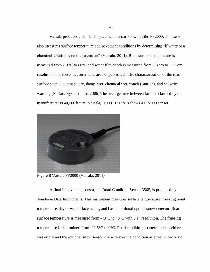
42
Vaisala produces a similar in-pavement sensor known as the FP2000. This sensor
also measures surface temperature and pavement conditions by determining “if water or a
chemical solution is on the pavement” (Vaisala, 2011). Road surface temperature is
measured from -51°C to 80°C and water film depth is measured from 0.3 cm to 1.27 cm;
resolutions for these measurements are not published. The characterization of the road
surface state is output as dry, damp, wet, chemical wet, watch (caution), and snow/ice
warning (Surface Systems, Inc. 2006) The average time between failures claimed by the
manufacturer is 40,000 hours (Vaisala, 2011). Figure 8 shows a FP2000 sensor.
Figure 8 Vaisala FP2000 (Vaisala, 2011)
A final in-pavement sensor, the Road Condition Sensor 3565, is produced by
Aanderaa Data Instruments. This instrument measures surface temperature, freezing point
temperature, dry or wet surface status, and has an optional optical snow detector. Road
surface temperature is measured from -43°C to 48°C with 0.1° resolution. The freezing
temperature is determined from -22.5°C to 0°C. Road condition is determined as either
wet or dry and the optional snow sensor characterizes the condition as either snow or no

43
snow (Aanderaa Data Instruments, 2010). Figure 9 shows the Road Condition Sensor
3565.
Figure 9 Aanderra Road Condition Sensor 3565 (Aanderaa Data Instruments, 2010)
Noninvasive Sensors
Non-invasive sensors are mounted apart from the road surface, either above the
roadway or at the roadside, and use spectroscopic methods, thermal radiation, and
infrared radar methods to determine surface weather conditions from a distance. Infrared
radiation and thermal radiation are measured to determine the temperature of the road
surface. Spectroscopic measures are used to determine roadway surface conditions (dry,
damp, wet, ice, etc.) remotely. Friction metrics can be calculated from the temperature
and surface conditions (Jonsson, 2010).
One non-invasive sensor, the NIRS31, is manufactured by Lufft. A pyrometer that
monitors thermal radiation is used to measure surface temperatures. Optical spectroscopy
is used to determine road surface conditions and water film depth on the roadway.
Friction is calculated based on the spectroscopic measurements taken. Road surface

44
temperature is measured from -40°C to 70°C with 0.1° resolution. The water film depth is
measured from 0 µm to 2000 µm with 10 µm resolution. The sensor’s own friction value
is calculated and given as a number between 0 and 1 with 0.01unit resolution. The road
condition is characterized as dry, damp, wet, snow/ice, or critical wetness (Lufft, 2011).
Figure 10 shows an NIRS31.
Figure 10 Lufft NIRS31 (Lufft, 2011)
Vaisala produces two non-intrusive weather sensors, the DST111 temperature
sensor and the DSC111 road condition sensor. The DST111 measures infrared radiation
to determine road surface temperatures. The DSC111 uses spectroscopic methods to
determine roadway conditions and water film depths. Road surface temperature is
measured from -40°C to 60°C with 0.1° resolution. The water film depth is measured
from 0 mm to 2 mm with 0.01 mm resolution. The friction is calculated and given as a
value between 0 and 1 with 0.01unit resolution. The road condition is output as dry,
moist, wet, snow/frost, ice, or slush (Vaisala 2010a, Vaisala 2010b). The DSC111 was
independently tested along with five other weather sensors, two non-invasive sensors,

45
and three in-pavement sensors, and was found to be reliable and recommended for use
above all others. The DSC111 was “very responsive toward changes in road surface
state” and the friction metrics determined by the sensor were found to be reasonable
when compared to a SAAB tire type friction tester for dry, wet and snowy conditions
(Jonsson, 2010). Figure 11 shows a DST111 with a DSC111. The reader should consult
the next section for more information on these sensors in use.
Figure 11 Vaisala DST111 (left) and DSC111 (right) (Vaisala 2010a, Vaisala 2010b)
Another noninvasive sensor that is manufactured by a Swedish company is known
as the Sensice ice detector. This sensor uses infrared spectroscopy to determine the
roadway conditions from three to 15 meters away. The sensor characterizes roadway
conditions as dry, wet, clear ice, snow, sleet, or wet clear ice. The sensor takes no direct
temperature measurements (Sensice, 2010). Figure 12 shows the Sensice ice detector.

46
Figure 12 Sensice Ice Detector (Sensice, 2010)
High Sierra Electronics produces a non-invasive sensor known as IceSight model
number 5433. This sensor utilizes laser and electro-optical technology to determine the
surface condition from up to 50 feet away. Monitoring near infrared spectral differences
allows the sensor to determine between different states of water on the road (water, snow
and ice). The reported sensitivity of the sensor is plus or minus 4°F for surface
temperature, plus or minus 1°F for ambient temperature, 0.01 inches of ice and water, and
0.05 inches for snow (High Sierra Electronics, 2011). Figure 13 shows the High Sierra
Electronics 5433 Sensor.
Figure 13 High Sierra Electronics 5433 Sensor (High Sierra Electronics, 2011)

47
Weather Sensors in Use
As part of a larger NCHRP report in 2006 on testing and calibration methods for
RWIS sensors, a survey of the use of pavement condition sensors was completed by
nineteen (19) state DOTs (SRF Consulting Group, 2006). It was found that 82% of the
responding states used the FP2000 sensor from Surface Systems Inc. (SSI), now Vaisala,
for roadway conditions (wet or dry). The three other sensors used were reportedly from
Vaisala, Nu-Metrics (now Vaisala), and one unidentified manufacturer.
A similar survey was administered by the Pennsylvania DOT for an investigation
into the future of RWIS (Gannett Fleming, Inc., 2007). This survey was completed by 26
state DOTs. Fifty percent of respondents reportedly use some Vaisala equipment, 36
percent used Quixote (now Vaisala) equipment, and 73 percent used SSI (now Vaisala)
equipment. Eighty-eight percent of respondents indicated the sensors were being used to
measure road surface condition (wet or dry).
Specific examples of non-invasive sensor use included the Vaisala DSC111
sensor being used in Yakima County, Washington; Aurora City, CO; North Dakota;
Virginia; Alaska; British Columbia; Quebec; Ontario; Finland; Sweden; UK; and
Germany (the specific use of these sensors was not indicated by the vendor, but it could
be assumed to be surface state and friction) (Vaisala, 2006). These reported users of the
DSC sensor have been reported by Vaisala and have provided data that shows positive
accuracy and reliability characteristics from the sensor’s deployment. The reader is
cautioned however that these optimistic reports are provided by the equipment vendor,
not an unbiased third party evaluator.

48
A project conducted by the Aurora pooled fund (an international partnership of
public agencies performing studies of RWIS) in Ontario and North Dakota was
conducted to determine the accuracy and usefulness of the Vaisala DSC111 and DST111
(Aurora, 2010). The project compared DSC111 data to an existing in-pavement sensor
(Lufft IRS31) and friction data to a Traction Watcher One friction tester and a Halliday
RT3 friction tester. Results indicated that the DSC111 sensor outputs for temperature
and surface condition (wet, dry, etc.) were comparable to the in-pavement sensors. The
friction testing results were vague and concern was noted for the DSC111’s friction data
at low friction ranges.
Federal Guidance
Recently the Federal Highway Administration (FHWA) has published a report
containing guidance for the use of VSL systems in wet weather (Katz et al., 2012). This
report contains a process that can be used to determine if a wet weather VSL system is
appropriate. This process includes a series of yes/no type questions in a flow chart to help
determine if a VSL system is justified. The proposed location must experience adverse
weather resulting in operational or safety issues, experience crashes at a rate higher than
expected for similar segments, have a regularly occurring requirement of at least a 10
mph drop in safe speed from posted speed limit, and possibly experience conditions
where stopping distance exceeds available sight distance for a wet weather VSL system
to be justified. Figure 14 shows the flowchart from the FHWA report.

49
Figure 14 Wet Weather VSL Flowchart (Katz et al., 2012)
Guidance for the use of regulatory versus advisory type VSL systems is also
included in this report. In general, regulatory systems are thought to result in higher speed
limit compliance rates. The legal authority of the highway agency to impose a regulatory
VSL in the proposed location is another consideration that must be made before
determining the type of system to be installed. Lastly, the report provides a general

50
guideline that if the road segment receiving the treatment is more than 2 miles long then a
regulatory VSL should be used; otherwise an advisory VSL should be used.
The report includes discussion about determining speed limits to be displayed
during certain situations. Currently there are no comprehensive algorithms for
determining speed limits during weather events, but the report references work performed
on the ODOT project that formed the basis of this thesis which will be presented in
Chapter 4 in the concept development. The report also provides a sample algorithm
meant to illustrate the kind of considerations that should be included for these systems.
This sample algorithm takes the road conditions, sight distance, and roadway grade into
account when setting appropriate speeds. Regardless of what method is used to adjust
speeds, the algorithm should be approved by a traffic engineering professional. The
lowest speeds that should be displayed on a freeway are given as 30 mph for a regulatory
speed limit and 15 mph for an advisory speed, and speeds should only be displayed in 5
mph increments.
Guidance about the signing and placement of signage for these VSL systems is
also discussed in the FHWA report. A system should monitor and provide real-time
weather information, but limit changes in the VSL posted speed to once every 60 seconds
so that drivers are not confused by rapidly changing signage. The signs should be placed
no more than 1 mile upstream of the location for the desired speed limit being displayed.
If VSL signs are used in a corridor, two consecutive signs (1 mile apart or less) should
not differ by more than 15 mph without advanced warning to drivers. Also the use of

51
dynamic message signs is encouraged to provide warning to drivers and credibility to the
VSL signage.
Conclusions
This chapter has summarized the literature pertaining to weather-responsive
variable speed limit systems, both in the U.S. and internationally, as well as other,
general VSL systems and federal guidance on the use of wet weather VSL systems.
Weather responsive VSL systems were used in a variety of applications (rain, fog, snow),
and primarily deployed on high volume roads. Different approaches were employed to
set posted speed limits for weather-responsive VSLs, including the use of set
algorithms/data processing, as well as manual observations where an operator changed
speed limits based on viewed conditions. In general, the weather-responsive systems
deployed to date have shown different, positive impacts on reducing crashes and
lowering speeds.
General VSL systems were found to be deployed by agencies to address a variety
of safety and operational issues. These systems relied on a variety of data inputs to
determine appropriate speed limits. This included loop detector data for speeds and lane
occupancy/traffic volumes, closed circuit television for manual observation, and other
inputs. The speed limits for each system were determined manually or automatically,
based on data inputs and the sophistication of the system itself. These general VSL
systems were typically shown to be effective when evaluations were made, although such
evaluations were not made for all systems.

52
The literature review also examined other weather-responsive systems that were
not necessarily VSLs, but did provide some form of motorist warning. These systems
were deployed to address different safety and operational concerns, using weather data to
activate different technologies, such as dynamic message signs, to provide information to
motorists. While specific speed limits were not set or provided by these systems, they
still were observed in general to be effective in lowering vehicle speeds and/or reducing
crashes.
Different types of weather sensors available for determining pavement conditions
(and in some cases, friction/grip) were also examined. Two general types of sensors are
available, invasive and noninvasive. Invasive sensors (in-pavement sensors) are installed
in the pavement level with the road surface and can use different sensing technologies in
determining conditions. Noninvasive sensors are installed on the roadside or somewhere
over the road surface and use non-contact means of monitoring weather and surface
conditions. During the course of the sensor review, it became apparent that Vaisala was
the primary vendor in the sensor market, and the firm’s DST111 and DSC111 system
appeared to hold promise for use in a weather-responsive VSL system. These sensors,
working in tandem, are capable of measuring roadway conditions (wet, snow, ice) and
water film depth, as well as temperature. They are also capable of measuring friction as a
value between 0 and 1, with 0.01 unit resolution. Such a measure is expected to be useful
in setting variable speed limits on highways, where different amounts of
moisture/precipitation can have a dramatic effect on pavement condition and friction.
Some limited independent testing found the system to be “very responsive toward
53
changes in road surface state” and friction metrics to be reasonable when compared to a
SAAB tire type friction tester for dry, wet and snowy conditions. Further testing
performed during this thesis research is presented in Chapter 5.
Federal guidance on the use of VSL systems in wet weather was also reviewed.
Specific guidance about situations were these systems may be justified was examined.
The FHWA report also outlines considerations about regulatory vs. advisory VSL
systems, how to develop speed change algorithms, and some specifics about the signs and
sign placement for different installations.

54
STUDY SITE CHARACTERIZATION
This chapter will introduce the study site and present the analysis of speed data
collected for the existing conditions as well as crash records and how local weather
impacts these site characteristics. This site was analyzed for its feasibility for a wet
weather VSL system implementation.
Description of Study Site
The proposed weather responsive VSL system was developed for the US
Highway 26 / OR Highway 217 Interchange in Beaverton, OR. Three ramps are included
in the potential VSL system: the US26 eastbound to OR217 southbound ramp, the US26
westbound to OR217 southbound ramp, and the OR217 northbound to US26 westbound
ramp. Figure 15 presents an overview of the project interchange and the respective
ramps.
Figure 15 US26 / OR217 Site (Base Image: maps.google.com)

55
Officials at ODOT identified the site, where over 60,000 vehicles per day
collectively use the interchange ramps, and once wet pavement conditions occur at this
site, crashes classified as “loss of control” increase. While the site has traditional passive
signage and flashing beacons in place, crashes continue to occur. ODOT personnel have
concluded that additional measures are necessary to address the problem.
All three ramps have advisory speeds posted 30 mph, but the regulatory speed
limit posted, on both the US26 and OR217 mainline segments, is 55 mph. All three ramps
have two lanes of traffic in the same direction. All three ramps begin with spiral curves
and transition to circular curves. These circular curves have the sharpest radius on the
ramps. The US26 eastbound to OR217 southbound ramp has a circular curve radius of
approximately 382 feet, the US26 westbound to OR217 southbound ramp has a circular
curve radius of approximately 266 feet, and the OR217 northbound to US26 westbound
ramp has a circular curve radius of approximately 318 feet.
Speed, Crash and Weather Data Analysis
In order to better understand the specific problems faced at the study site the
speed and crash data were analyzed and local weather was also investigated to see its
effect on the existing speeds and crash experience.
Data Sources and Overview
Speed data was collected by the ODOT on all three ramps during the months of
December 2011 and January 2012. Individual vehicle measurements were recorded
including the date, time, speed, headway, acceleration, and vehicle classification

56
information for every vehicle travelling on the ramps during the two month study period.
Road tube type vehicle counters were used to collect vehicle data near the point of
curvature of the most restrictive portion (sharpest radius) curve on the ramp.
Crash data for the three freeway ramps being investigated was gathered from state
highway crash reports compiled from individual driver and police crash reports submitted
to ODOT as required by state law. The Crash Analysis and Reporting Unit of the
Transportation Development Division of ODOT maintains these records online at
https://keiko36.odot.state.or.us/ under the Crash Data System tool.
Weather data was gathered using the MesoWest weather website created and
maintained by the University of Utah, online at mesowest.utah.edu/. This tool was used
to download weather data from a Meteorological Assimilation Data Ingest System
(MADIS) station located near the study site. Additional historical weather data was
gathered from www.weatherbase.com, which utilizes records from the National Climactic
Data Center which is part of the National Oceanic and Atmospheric Administration
(NOAA).
Speed Data Methods and Results
The speed data was initially reduced to only include vehicles with headways of at
least 6 seconds. This was done so that only the motorists that chose their desired speed
would be included. Vehicles with small headways that are stuck following the vehicle
ahead are excluded because they may have desired to operate at a higher speed but were
limited by the vehicle ahead of them. The remaining vehicles represent the free flow
speed of the facility, because these vehicles chose their operating speed and were not

57
encumbered by slow moving traffic. The raw speed data that was collected included over
2 million individual vehicle records each with date, time, speed, headway, acceleration,
and vehicle classification information. After reducing the data to include only the free
flowing vehicles over 193,000 individual vehicle records remained.
The weather data collected included date, time, air temperature, relative humidity,
wind speed and direction, and precipitation amounts. These measurements were recorded
every 15 minutes and the two study months resulted in over 5,100 individual weather
records. The precipitation information was used to define dry periods and wet periods.
Dry periods were defined as times with no precipitation recorded in the past 24 hours.
Wet periods were defined as times with increasing amounts of measurable precipitation
(1 mm/hr or 0.04 in./hr) for at least 5 consecutive 15 minute periods.
The average speed and 85th
, 90th
and 95th
percentile speeds were calculated for dry
and wet conditions during both day and nighttime driving situations for all three ramps.
Safe speed was determined from ODOT design guides (ODOT, 2003) which utilize the
same equation and methods as those found in the American Association of State
Highway and Transportation Officials (AASHTO) “A Policy on Geometric Design of
Highways and Streets” commonly referred to as the AASHTO green book. Relative
speed frequency distribution charts were also created to better understand the existing
speed conditions at the site. Table 5 shows the speed characteristics that exist on the
US26 eastbound to OR217 southbound ramp.

58
Table 5 Basic Site Speed Characteristics for US26 EB to OR217 SB
East to South Ramp
Surface Dry Dry Wet Wet
Lighting Day Dark Day Dark
Number of Observations 27,786 27,928 7,288 1,901
Mean Speed (mph) 42.2 41.1 41.8 40.7
85th
Percentile Speed (mph) 47 46 47 45
90th
Percentile Speed (mph) 48 47 47 47
95th
Percentile Speed (mph) 50 49 49 48
Advisory Speed 30
Safe Speed 33
Mean speeds for all conditions exceeded the posted advisory speed by more than
10 mph. The 85th
percentile speeds for all conditions exceed the posted advisory speed by
15 mph or more.
Statistical tests were performed to determine if the differences in mean speeds
between the different weather and lighting conditions were significant. A two-tailed F-
test (with 95% confidence level) was first performed between two different conditions
(for example: dry day and wet day). This F-test determines if the variances of the two
populations are equal or not equal. Then, depending upon the results of the F-test, the
corresponding two-sample t-test (either using equal or unequal variances) was performed
to determine if the difference in mean speeds is statistically significant (Sheskin, 2000).
Table 6 shows the mean speed differences and statistical significance for the US26
eastbound to OR217 southbound ramp.

59
Table 6 Mean Speed Differences for US26 EB to OR217 SB
East to South Ramp
Conditions Dry Day Dry Dark Wet Day Wet Dark
Dry Day NA 1.1* 0.4* 1.5*
Dry Dark -- NA 0.7* 0.4*
Wet Day -- -- NA 1.1*
Wet Dark -- -- -- NA
* Indicates statistically significant difference at 95% confidence level
All differences were found to be statistically significant, but the magnitude of the
differences was small. The difference in mean speed due to lighting (both during dry and
wet conditions) was 1.1 mph. The difference in mean speed due to weather conditions
(both during day and dark conditions) was 0.4 mph.
The relative speed frequency distribution chart was created to check that the speed
distributions were approximately normal and did not include potentially dangerous
bimodal tendencies. Figure 16 shows the speed frequency distribution for the US26
eastbound to OR217 southbound ramp.
Figure 16 Speed Frequency Distributions for US26 EB to OR217 SB

60
Table 7 shows the speed characteristics that exist on the US26 westbound to
OR217 southbound ramp.
Table 7 Basic Site Speed Characteristics for US26 WB to OR217 SB
West to South Ramp
Surface Dry Dry Wet Wet
Lighting Day Dark Day Dark
Number of Observations 35,070 32,607 8,612 2,538
Mean Speed (mph) 40.8 39.1 40.0 38.3
85th
Percentile Speed (mph) 44 43 44 43
90th
Percentile Speed (mph) 46 44 45 43
95th
Percentile Speed (mph) 47 46 47 45
Advisory Speed 30
Safe Speed 28
Mean speeds for all conditions exceeded the posted advisory speed by more than
8 mph. The 85th
percentile speeds for all conditions exceed the posted advisory speed by
13 mph or more.
Table 8 shows the mean speed differences and statistical significance for the
US26 westbound to OR217 southbound ramp.
Table 8 Mean Speed Differences for US26 WB to OR217 SB
West to South Ramp
Conditions Dry Day Dry Dark Wet Day Wet Dark
Dry Day NA 1.7* 0.8* 2.5*
Dry Dark -- NA 0.9* 0.8*
Wet Day -- -- NA 1.7*
Wet Dark -- -- -- NA
* Indicates statistically significant difference at 95% confidence level
All differences were found to be statistically significant, but the magnitude of the
differences was small. The difference in mean speed due to lighting (both during dry and

61
wet conditions) was 1.7 mph. The difference in mean speed due to weather conditions
(both during day and dark conditions) was 0.8 mph.
Figure 17 shows the relative speed frequency distribution for the US26 westbound
to OR217 southbound ramp.
Figure 17 Speed Frequency Distributions for US26 WB to OR217 SB
Table 9 shows the speed characteristics that exist on the OR217 northbound to
US26 westbound ramp.
Table 9 Basic Site Speed Characteristics for OR217 NB to US26 WB
North to West Ramp
Surface Dry Dry Wet Wet
Lighting Day Dark Day Dark
Number of Observations 21,281 21,962 5,345 1,651
Mean Speed (mph) 42.1 40.6 41.6 40.2
85th
Percentile Speed (mph) 47 45 46 44
90th
Percentile Speed (mph) 48 47 47 46
95th
Percentile Speed (mph) 50 48 49 47
Advisory Speed 30
Safe Speed 30

62
Mean speeds for all conditions exceeded the posted advisory speed by more than
10 mph. The 85th
percentile speeds for all conditions exceed the posted advisory speed by
14 mph or more.
Table 10 shows the mean speed differences and statistical significance for the
OR217 northbound to US26 westbound ramp.
Table 10 Mean Speed Differences for OR217 NB to US26 WB
North to West Ramp
Conditions Dry Day Dry Dark Wet Day Wet Dark
Dry Day NA 1.5* 0.5* 1.9*
Dry Dark -- NA 1.0* 0.4*
Wet Day -- -- NA 1.4*
Wet Dark -- -- -- NA
* Indicates statistically significant difference at 95% confidence level
All differences were found to be statistically significant, but the magnitude of the
differences was small. The difference in mean speed due to lighting (both during dry and
wet conditions) was approximately 1.5 mph. The difference in mean speed due to
weather conditions (both during day and dark conditions) was approximately 0.5 mph.
Figure 18 shows the relative speed frequency distribution for the OR217
northbound to US26 westbound ramp. The relative speed frequency distribution chart
again showed the speed distributions to be approximately normal.

63
Figure 18 Speed Frequency Distributions for OR217NB to US26 WB
Speed Analysis
The results of the speed study show that potentially dangerous speed conditions
exist at the site. The safe speed is exceeded by the average speed at all three ramps by 7
to 10 mph during wet conditions. The differences in average speeds for dry and wet
pavements were found to be statistically significant, but only 0.4 to 0.8 mph in magnitude
for the three ramps. This shows that the motorists using these ramps do not slow down by
more than 0.8 mph on average when rainy conditions occur. This slight decrease in speed
may not be sufficient to safely navigate the ramps especially considering the average
speeds during wet conditions are still well above the safe speeds for the ramps.

64
Crash Data Methods and Results
Crash data was collected for five years (2007 through 2011). This included 119
total crashes (not including work zone related crashes) for the three study ramps. To
determine how often the pavement was likely to be wet during a typical year, historical
data and the two months of detailed study data were used. It was estimated that on a
given day in Beaverton, OR when rain occurs the pavement will be wet approximately
15% of that day. This was calculated from the two months of detailed study data for
every 15 minute period, which included 24 individual rain events lasting for at least 5
consecutive 15-minute periods. Then the historical weather data was used to determine
average number of days with rain in each month. Combining these two measures allows
for an estimate of the amount of time the pavement is wet for each month and the year
overall. See Appendix A for calculation details from this chapter. This investigation
resulted in the finding that the pavement is wet approximately 6% of the year, but over
the past 5 years 63% of crashes at the three ramps have occurred during wet conditions.
See Appendix A for detailed crash summaries.
To determine if these ramps have higher crash rates than other interchange ramps
the number of crashes per million entering vehicles (MEV) was calculated for each ramp.
The AADT for each ramp (published by the Oregon DOT) was used to determine the
number of entering vehicles. Table 11 shows the crash characteristics for the ramps.
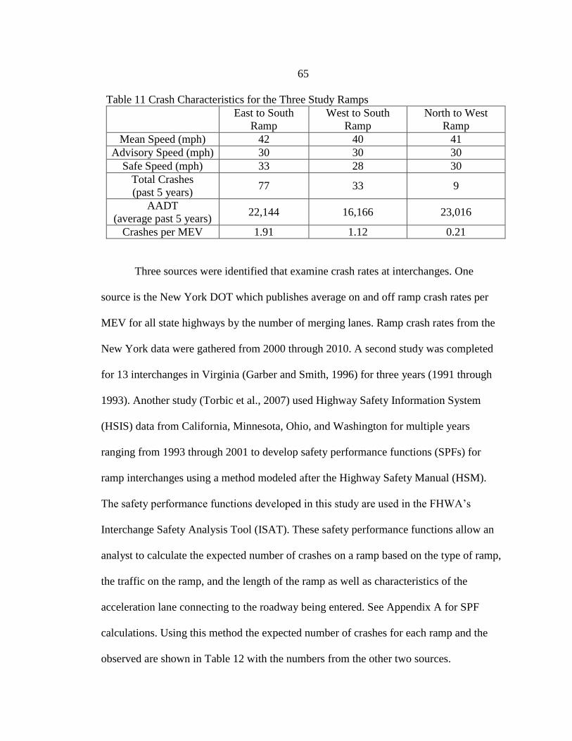
65
Table 11 Crash Characteristics for the Three Study Ramps
East to South
Ramp
West to South
Ramp
North to West
Ramp
Mean Speed (mph) 42 40 41
Advisory Speed (mph) 30 30 30
Safe Speed (mph) 33 28 30
Total Crashes
(past 5 years) 77 33 9
AADT
(average past 5 years) 22,144 16,166 23,016
Crashes per MEV 1.91 1.12 0.21
Three sources were identified that examine crash rates at interchanges. One
source is the New York DOT which publishes average on and off ramp crash rates per
MEV for all state highways by the number of merging lanes. Ramp crash rates from the
New York data were gathered from 2000 through 2010. A second study was completed
for 13 interchanges in Virginia (Garber and Smith, 1996) for three years (1991 through
1993). Another study (Torbic et al., 2007) used Highway Safety Information System
(HSIS) data from California, Minnesota, Ohio, and Washington for multiple years
ranging from 1993 through 2001 to develop safety performance functions (SPFs) for
ramp interchanges using a method modeled after the Highway Safety Manual (HSM).
The safety performance functions developed in this study are used in the FHWA’s
Interchange Safety Analysis Tool (ISAT). These safety performance functions allow an
analyst to calculate the expected number of crashes on a ramp based on the type of ramp,
the traffic on the ramp, and the length of the ramp as well as characteristics of the
acceleration lane connecting to the roadway being entered. See Appendix A for SPF
calculations. Using this method the expected number of crashes for each ramp and the
observed are shown in Table 12 with the numbers from the other two sources.

66
Table 12 Crash Rates for the Three Study Ramps
East to South
Ramp
West to South
Ramp
North to West
Ramp
Observed
(crash/MEV) 1.91 1.12 0.21
NY DOT Average
(crash/MEV) 0.10 0.10 0.07
Virginia Study Average
(crash/MEV) 0.24 0.24 0.09
Expected from SPF Study
(crash/MEV) 0.21 0.26 0.24
Crash Analysis
One of the FHWA guidelines for VSL systems in wet weather is to investigate if
the proposed location has a crash rate higher than expected for similar segments. The
results show that the East to South ramp has a crash rate of 1.91 crashes per MEV which
is considerably higher than all three crash rates identified in the literature. The West to
South ramp experienced a lower crash rate compared with the East to South ramp;
however, it is still much higher than the three crash rates found in the literature. The
North to West ramp has a much lower crash rate compared with the previous two ramps,
but slightly lower than the expected crash rate identified from the SPF literature, and
somewhat higher than the rates from the other two state studies.
Conclusions
The study site speed, crash and weather data analyses suggest that this location
experiences speeds that are considerably higher than the safe operating speeds during
adverse weather events. The crash analysis shows that two of the three study site ramps
experience crash rates higher than crash rates found in the literature. Weather records
show that the pavement at the study site is wet about 6% of the time averaged for the

67
entire year, yet over 60% of crashes at the site occur during wet weather. Speed and
weather data show that drivers reduce their average speeds during wet weather, but only
less than 1 mph. This suggests that some driver may slow down as they navigate the
interchange during wet weather, but many may not reduce their speeds when using these
interchange ramps in the rain. Average speeds show that drivers operate at 7 to 10 mph
above safe speeds even during wet weather conditions. These findings suggest that a
weather responsive VSL system may be useful at this location to influence driver
behavior and achieve lower average speeds during wet weather conditions.

68
WEATHER RESPONSIVE VSL: CONCEPT DEVELOPMENT
This chapter will present the development of the proposed VSL system for the
study site. The purpose of the system and a detailed concept of operations will be
presented including a general system concept, system overview and operational
scenarios.
Purpose of Proposed System
The previous chapter has shown the existing speed problems present at the study
site, especially during wet weather conditions. This project seeks to reduce the
occurrence of wet weather crashes on the three study ramps of the US26/OR217
interchange through the use of a weather responsive variable speed limit system. This
system is a unique example of VSLs as no other weather responsive VSL systems have
been targeted specifically for interchanges. Such a system will post appropriate speed
limits based on weather conditions, with the intent of lowering motorists’ speeds
accordingly. The system will also incorporate active warning signs in the form of
dynamic message signs to provide advanced warnings to motorists upstream of the
ramps. As motorists lower their speeds for different weather conditions, they will be
traveling at safer speeds for prevailing conditions, with a corresponding reduction in
crash occurrence expected.

69
Concept of Operations
The concept of operations developed for the study site includes an overall system
concept detailing the applicable weather sensors and signage. Additionally, the system
overview that presents the logical architecture, thresholds for changing speeds, and the
system control is included in this section along with operational scenarios.
System Concept
The concept of the VSL system is to adjust the speed limit on the interchange
ramps during inclement weather to influence driver behavior – primarily to reduce speeds
based on the presence of wet pavement. Using pavement condition and weather sensors at
the site, different road weather conditions can be detected and verified. Based on the
current road weather and pavement conditions at the site, speed limits can be adjusted
accordingly using VSL signs. The operation of the system will involve this general
sequence of events:
Weather and non-invasive pavement sensors monitor precipitation occurrences,
type, accumulations, pavement temperature, ambient temperature, and an
estimation of grip level of the surface of the roadway.
Road condition changes are identified based on the detected conditions processed
by the system controller, using threshold values determined by the system
algorithm developed prior to deployment.
Upon identification of changes in current conditions, the system logic
automatically changes the signage for the desired control strategy (e.g. change
from advisory speed of 30 mph to regulatory posted speed limit of 25 mph).

70
The system continuously monitors current conditions, compares those conditions
to the established threshold values, determines control strategies/speed limits, and
implements necessary changes in signage.
Weather Sensors. Sensors that focus on the condition of the pavement on the
roadway are of interest to this type of system and come in two major styles: in-pavement
and non-invasive. In-pavement sensors are puck shaped sensors that are set in the
roadway and can measure pavement temperature, precipitation occurrences, precipitation
type, and depth of precipitation. Non-invasive sensors use spectroscopic principles to
measure road surface conditions from above the roadway. Non-invasive sensors can
measure pavement temperature, precipitation occurrences, type, and depth and give an
estimate of the level of grip of the pavement. Non-invasive sensors which provide
information on both pavement condition and grip are to be used in the system presented
here.
Wet and extreme weather crashes likely occur on the interchange ramps due to a
loss of grip between the wet pavement and vehicles travelling too fast for the conditions
of the roadway. To monitor when the roadway exhibits potentially dangerous conditions,
sensors will need to monitor precipitation occurrences, type, depth, and pavement
temperatures. Grip levels can only be measured by non-invasive sensors, and this is why
such a pavement condition sensor has been selected as the primary sensor for the VSL
system. Chapter 5 presents more information on the non-invasive sensor selected for use
in the proposed system and testing results related to its capabilities.

71
Variable Speed Limit Signs. The VSL signs will be installed at the beginning of
the three ramps being investigated (US26 EB to OR217 SB, US26 WB to OR217 SB, and
OR217 NB to US 26 WB). The signs will be placed on the roadside(s) where sufficient
space is available. Regulatory VSL signs will be placed at the point of curvature (POC)
of the ramps and the advisory sign with LED numbers will be placed 100 feet upstream
of the POC. Figure 19 shows a typical ramp geometry with POC and a location 100 feet
upstream of the POC identified as potential sign locations. The figure also shows the
existing locations for the exit and advisory speed signs. The existing advisory speed signs
will be removed upon the deployment of the proposed VSL system.
Figure 19 Potential Sign Placement

72
VSL Sign Types. Two types of VSL sign are proposed for use as part of this
project. One type is a full matrix type variable electronic sign. The other is a more
traditional static background sign with a light emitting diode (LED) panel that changes
only the numerical speed part of the sign. The following graphics presented are only for
demonstrating the possible signage and the physical sign details including shapes and
fonts would need to conform to MUTCD guidelines.
A full matrix variable electronic sign is capable of displaying an electronic
version of static signage as well as dynamic flashing graphics (ex. simulated flashing
beacons above a static sign). For the purposes of this project, the sign will have the ability
to display a regulatory speed limit sign with any numerical speed in the appropriate
colors that conform to MUTCD guidance. When the sign is not activated, (i.e. when an
advisory speed limit is in effect during dry conditions), the electronic sign will be blank
(blacked out) and convey no information. Figure 20 shows an example of the electronic
full matrix VSL signage with the ODOT specific template omitting the word “limit”.
Figure 20 Electronic VSL Sign Example

73
The regulatory electronic VSL signs will be placed on the right side of the road at
the point of curvature of the ramps. This point of curvature is the start of the most
restrictive curve encountered by the driver using the ramp.
A static background curve warning sign attached to a dynamic advisory speed
sign with LEDs is proposed for the system to work in coordination with the full matrix
regulatory VSL sign described previously. Such warning / advisory signs would be a
traditional static warning sign similar to those already present on the ramps that displays
the ramp geometry on the metal portion of the sign and the advisory speed limit on a
changeable LED sign attached below the metal sign. The static portion of the sign would
always display the ramp geometry since it has no electronic features, but the LED speed
would only be displayed when applicable and would be blank when not activated. Figure
21 illustrates this sign, showing the static background with LED advisory VSL signage
below it.
Figure 21 Static Background Advisory with LED VSL Sign Example

74
The advisory speed signs will be placed at the roadside at 100 feet upstream from
the regulatory VSL signs. This conforms to the MUTCD recommendations that advisory
warning signs be up to 100 feet upstream of the point of curvature of a ramp and at least
100 feet from any other signs.
An alternative signage layout is possible for the ramps utilizing only the full
matrix variable electronic signs. These signs are capable of displaying many colors and
virtually any shapes, therefore a single electronic sign could be used for both the
regulatory and advisory / geometric signage. This alternative using only one electronic
sign could then be placed at either potential sign location. Figure 22 shows the alternative
electronic VSL sign example.
Figure 22 Alternative Electronic VSL Sign Example
Advanced Warning Signs. Advanced warning signs will be used sufficiently
upstream of the ramps to notify drivers that they may encounter a reduced speed limit
zone ahead. These signs would be Dynamic Message Signs (DMS) and only activated

75
when the reduced speed limit zone is in effect on the ramps being investigated. The sign
would display a message predetermined by ODOT to alert drivers on the ramps that they
are approaching the reduced speed limit zone. The DMS should be equipped with
flashing beacons, either within the border of the DMS or externally attached to the sign to
capture driver attention. These beacons will flash only when reduced speed limits are in
effect. Figure 23 shows an example of potential advanced warning sign and posted
message.
Figure 23 Advanced Warning Sign Examples
System Overview
The VSL system will be controlled by software that will use an algorithm to
determine recommended speeds. The algorithm will determine appropriate speed limits
during different pavement and weather conditions. The possible weather conditions are:
dry pavement with no rain, light to moderate precipitation with minor reductions in
pavement grip, and heavy precipitation with significant reductions in pavement grip. The
VSL speed control software employed in the system will comply with the applicable
standards and procedures for changing speed limits on Oregon freeways. The system
will:
not change speed limits more than once every 5 minutes,
not display a speed limit below 20 mph,

76
only display speed limits in 5 mph increments, and
automatically assess weather conditions every 60 seconds.
Logical Architecture. The VSL system is comprised of three separate systems,
one for each ramp. Each individual ramp VSL system will address its ramp-specific
pavement and weather conditions and display the appropriate speed limit. Pavement and
weather conditions will be monitored at each ramp and speed limits will be assigned
according to weather conditions. One centralized controller will be employed by the
system, while individual condition detection sensors will be used on each ramp. The
multiple sensors may allow for the system to perform quality control checks on other
individual sensors to ensure that a sensor is not malfunctioning or outputting poor quality
data.
Thresholds for Changing Speeds. Weather conditions are determined from the
pavement and weather sensor data. This data will be assessed at 60 second intervals and
appropriate changes in the type (advisory versus regulatory) and speed posted by the
signage will be determined. The system will need to perform consistency checks over a 5
to 10 minute period to confirm weather / pavement conditions. The major weather
condition categories will be:
1: dry pavement, no precipitation, high grip level
2: moist / wet pavement, light precipitation, moderate to high grip level
3: wet pavement, moderate to high precipitation, moderate grip level
4: ice/snow/slush/frost pavement, any precipitation, low grip level

77
Table 13 shows potential weather measurements that correspond to the categories 1
through 4. These categories and corresponding thresholds are based on sensor testing
results included in Chapter 5: Sensor Testing.
Table 13 Weather Condition Classification
Precipitation Precipitation
Depth (mm) Grip Reading
Condition
Category
Dry N/A > 0.80 1
Moist / Wet < 1.00 0.70 to 0.79 2
Wet > 1.00 0.50 to 0.69 3
Ice / Snow / Slush / Frost Any Any 4
Figure 24 shows the general logic used to determine appropriate control signage
strategies at a given ramp. The weather sensor will communicate measurements to the
processor which will use the system logic and surface condition categories to determine
the appropriate signage to be posted. The processor will communicate the desired signage
to the VSL signs. The signs will display the necessary information for the conditions. The
system will reassess the surface condition every 60 seconds and change the signage
accordingly, but no more often than once every 5 minutes.
The three ramps all currently have a posted advisory speed of 30 mph. Reduction
in posted speed limits will be in 5mph increments but will never be posted lower than 20
mph. Table 14 shows the potential signs and speeds posted from the logic determined
weather condition category.
Table 14 Condition, Sign, and Speed
Condition Advisory VSL Regulatory VSL Speed Posted
1 ON OFF 30
2 ON OFF 30
3 OFF ON 25
4 OFF ON 20

78
Figure 24 System Logic Schematic
System Control. The existing TMOC in Portland, OR will operate and oversee the
VSL system. Changes in road weather conditions will be detected automatically and
appropriate speeds will be posted without the need for direct operator involvement. The
operator will be informed of changing road weather conditions by alarms triggered when

79
posted speed limit changes are warranted. Incidents will be monitored by the operator
using radio communication, telephone calls, and from CCTV cameras at or near the site.
The operator may expect to first receive an alarm of lowered speed limit, observe
automatic speed limit change being posted (via system outputs, not CCTV), and verify
the weather conditions using the existing on site camera, and any other cameras that may
be added at the project site. The system will have three primary operational modes: test
mode, normal mode, and manual operation.
The VSL system will have the option to operate in a test mode. This test mode
will operate the same way as normal operation, except it will not post the speeds
determined from the algorithm. During the test mode, operators can observe the system
as it operates and see the sign changes that are suggested by the processor, but the sign
changes will not be shown in the field. This mode will allow operators to ensure the
system is functioning properly before allowing the automatic speed changes to be
implemented and presented to drivers.
Normal operation of the VSL system will be employed once TMOC operators are
satisfied that the system is operating correctly in the test mode. The system will analyze
the weather measurements from the sensors, check the data against the system algorithm
and threshold conditions, and automatically post the appropriate sign changes. An alarm
will be triggered to inform TMOC operators of speed limit changes and confirm weather
conditions, if desired.
If desired, a TMOC operator can override the normal operation of the system and
engage a manual operation mode. Using manual operation mode, the operator can choose

80
to post any speed limit signage they feel appropriate for the conditions. Note, however,
that such an operation should not be undertaken except in the case of a severe event or
emergency. In such a case, local police or ODOT personnel in the field may also be
consulted for input prior to performing any manual operation of the system. For
example, an incident on the ramp (stall or crash) may necessitate a change in the posted
speed limit that would not be triggered by weather conditions. Automatic signage
changes from the VSL system processor will be suspended until the operator resumes
normal operation mode. The VSL system will continue to monitor conditions and log
suggested signage conditions. An alarm may also be used to inform operators in the event
that the VSL system suggests a lower speed than manual operation currently has set.
Operational Scenarios
The possible operational scenarios for the VSL system include:
Dry Pavement Operations
o Condition 1
Wet or Extreme Pavement Operations
o Condition 2
o Condition 3
o Condition 4
Failure Operations
o Detection Failure
o Entire System Failure

81
Operational Scenario: Condition 1. When the site experiences dry conditions and
sensors measure no precipitation and high grip levels, operations will be classified as
condition 1. Under condition 1, the variable advisory speed sign will display 30 mph and
the regulatory VSL will be blank. The DMS will be blank as there is no reduction in
speed limit for the driver to anticipate. Figure 25 shows the signage displayed during
condition 1 operations.
Figure 25 Condition 1 Operations
Operational Scenario: Condition 2. When the site experiences light precipitation
and sensors measure light precipitation with moderately high grip levels (i.e. good grip
values in the presence of pavement moisture), operations will be classified as condition 2.
Under condition 2, the variable advisory speed sign will display 30 mph and the
regulatory VSL sign will be blank. The DMS will be blank as there is no reduction in

82
speed limit for the driver to anticipate. Figure 26 shows the signage displayed during
condition 2 operations.
Figure 26 Condition 2 Operations
Operational Scenario: Condition 3. When the site experiences precipitation and
sensors measure some precipitation with mid-range grip levels, operations will be
classified as condition 3. Under condition 3, the regulatory VSL sign will display 25
mph. The variable advisory speed sign will be blank. The DMS will display a reduced
speed limit ahead notification for drivers using the ramps. Figure 27 shows the signage
displayed during condition 3 operations.

83
Figure 27 Condition 3 Operations
Operational Scenario: Condition 4. When the site experiences icy, snowy, slushy,
or frosty conditions and sensors measure ice, snow, slush, or frost precipitation with any
grip level, operations will be classified as condition 4. Under condition 4, the regulatory
VSL sign will display 20 mph. The variable advisory speed sign will be blank. The DMS
will display a reduced speed limit ahead notification for drivers using the ramps. Figure
28 shows the signage displayed during condition 4 operations.

84
Figure 28 Condition 4 Operations
Operational Scenario: Detection Failure. When the system experiences a single
sensor/detector/component failure, other than the VSL sign, TMOC operators will be
informed that a failure has occurred and can choose to manually operate the VSL sign or
have the system automatically operate the VSL sign using the weather conditions from
one of the other ramp’s sensors.
Operational Scenario: Entire System Failure. If the entire VSL system fails in
some manner, operators will be notified and drivers will only observe the static advisory
geometry sign, as all LED boards will be blank. This may happen in the event of a power
outage at the site, absent power from backup batteries. Both the regulatory and advisory
VSL signs will be blank, but the ramp geometry advisory static metal sign will be
observed by drivers on the ramps. The DMS will also be blank. Such a case would
require ODOT personnel to travel to the site to set up temporary static metal signage

85
displaying an advisory or regulatory speed limit. Figure 29 shows the signage displayed
in the event of an entire system failure.
Figure 29 Entire System Failure Operations

86
SENSOR TESTING
This chapter will present the methods, results, and analysis of the non-invasive
sensor testing performed during the project.
Introduction
In practice, road weather sensors are often used as part of Road Weather
Information System (RWIS) stations, and to a lesser extent, as components of the recent
weather responsive advanced transportation applications. Examples these weather
responsive systems are the safety warning systems for inclement weather conditions (ice,
wind, fog, etc.) using Dynamic Message Signs (DMS) and the weather-responsive
variable speed limit (VSL) systems which adjust the posted speed limit under different
weather and road surface conditions (Veneziano and Ye, 2011, Ulfarsson et al., 2001).
With the advances in sensor, communications and control technologies, these and similar
applications are expected to increase in the foreseeable future.
The non-invasive road weather sensors employ relatively new technology that is
less proven than the older, more common in-pavement road weather sensors. In the
course of this research, only a few manufacturers were identified as producers of non-
invasive road weather sensors with capabilities that meet the requirements of the
proposed application. However, other than manufacturer’s literature and website
information, no independent studies have been identified to test the capabilities of the
sensors and consequently the reliability of using sensor outputs in automated ITS
applications. The only exception to the previous statement was the Vaisala weather

87
sensors that were selected in this research project for the VSL application. A few studies
were conducted to test the sensors that are described next in this section.
For road weather conditions, Vaisala offers two weather sensors, the remote road
surface state sensor (DSC-111) and the remote road surface temperature sensor (DST-
111). The two sensors that are used in combination have been in the market for the last
few years and were tested in a few studies. Two studies were conducted by Aurora,
which is an international partnership of public agencies performing joint research,
evaluation, and deployment initiatives related to road weather information systems
(http://www.aurora-program.org/index.cfm). These two studies attempted to examine the
Vaisala sensors by installing the sensors in the field and comparing sensor outputs with
data gathered from in situ sensors to determine if the data were accurate.
The first study was conducted east of Ottawa in Ontario, Canada (Feng and Fu,
2008). This study found that the Vaisala sensors were reliable and accurate in
determining road surface state and that there were systematic differences in temperature
measurements between the Vaisala sensor and the in-situ sensor used in the study.
Further, the grip levels reported by the Vaisala sensor did not correlate well with the
friction coefficients measured by a friction meter at the same location and time interval,
especially under conditions of low friction. The study concluded that the DSC-111 cannot
be used as a reliable replacement of friction measuring equipment.
The second Aurora study was conducted in North Dakota (Tilley and Johanneck,
2008) adjacent to Interstate 29 south of Grand Forks. The study found that the Vaisala
sensor suite produced results, with respect to pavement temperature, that were

88
comparable to current in situ technologies and that fog could impact the Vaisala sensor
temperature readings. Also, the sensor was reportedly able to determine the pavement
conditions reasonably well compared to camera images of the road surface.
A third field study of the sensor was performed in Sweden (Jonsson, 2010). The
testing found the sensor to be accurate at determining the surface condition of the
pavement. Friction estimates reported by the sensor we also found to be reasonable when
compared to the wheel type friction tester used for comparison. The snow depth
measurements were found to be inaccurate. Overall conclusions stated the sensor showed
promise for further testing and use.
The objective of this study is to test the ability of the Vaisala non-invasive
weather sensors DSC-111 and DST-111 in measuring weather parameters that are of
interest to the proposed VSL system. The tests and validations that were reported in the
literature and summarized above are limited in a sense that they either compared the
sensor’s outputs to their counterparts from other in-pavement weather sensor
technologies or considered only limited weather parameters in their testing. The current
study examines four important weather parameters namely: pavement surface state, water
depth, ice and snow depth and the grip level. The study tests the accuracy of the sensor
outputs relevant to the actual values measured in a controlled laboratory environment.
This testing is expected to provide a more accurate assessment of the capabilities and
limitations of the Vaisala weather sensors for the proposed VSL or other similar ITS
applications.

89
Testing Methods and Results
The sensor testing in this study involved four important road weather parameters
that are estimated by the weather sensors. These include surface state, tire-pavement grip
level, snow and ice depth and water depth. The following sections describe each of these
individual tests summarizing methodology, experimental design and the most important
results and findings.
Surface State
The sensor’s ability to determine the surface state of the roadway was tested. The
manufacturer reports that the sensor can determine the road condition as dry, moist, wet,
frosty, snowy, icy, or slushy.
The surface state determination testing was performed at the Montana State
University (MSU) Subzero Science and Engineering Research Facility in Bozeman,
Montana. This research facility has a number of large, walk-in environmental chambers
(cold labs) that can be programmed to precise temperatures for testing. This allowed for
sensor tests to occur under different temperature conditions in a fully controlled
environment.
The sensors were secured atop a tripod set up in the cold lab and connected via an
RS-232 communications cable to a laptop placed outside the lab. The free data terminal
program PuTTY was used to send commands to and receive data from the sensors.
The sensors were positioned so that the measuring distance to the pavement
samples was approximately 3 meters and the installation angle was approximately 37
degrees. The sensor installation angle is the angle measured from the horizontal road

90
surface up to the sensor line of sight. This set-up complies with the limits for installation
published by the vendor, fits within the cold lab, and ensures that the DSC-111’s
measurement ellipse was appropriately sized based on the dimensions of the pavement
samples. Specifically, the measuring distance of the sensors must be between 2 and 15
meters from the pavement, with an installation angle between 30 and 85 degrees
according to the manual. The measurement ellipse is the area on the sample that is
measured by the DSC-111, and this ellipse becomes larger as the measurement distance
increases. The DSC-111 Aiming Tool Kit was used to position the pavement samples on
the floor to ensure they were being accurately measured.
One asphalt sample (9 inches wide, 20 inches long, and 1 inch thick) and one
concrete sample (12 inches wide, 16 inches long, and 2 inches thick) were used to
simulate roadway surfaces for testing. These samples were chosen from available
materials with appropriate dimensions for testing. A silicon barrier was added near the
outside edge of each sample to allow precipitation to pond on the surface of the samples.
The laboratory testing simulated a variety of surface conditions including dry,
moist, wet, covered with loose snow, covered with compacted snow, and ice with various
depths. The depths were chosen based on the reported capabilities of the DSC-111. As
suggested in the DSC-111 manual, the sensor was calibrated for the dry condition for
each sample before changing conditions. For each condition and corresponding pavement
sample, the DSC-111 output was monitored until the readings stabilized, at which time
the sensor readings were recorded. This stabilization takes at most 3 minutes and seems

91
to be a gradual change programmed into the sensor to avoid unrealistic jumps between
changing conditions.
The moist condition was considered to exist when the surface is visibly damp but
no standing water is present. Water was applied with a trigger type squirt bottle set to
spray a mist of water (not a stream of water). Wet samples with increasing water depth
were created by spraying multiple lifts of water and allowing the DSC-111 readings to
stabilize between lifts. Snow created by the Subzero Science and Engineering Research
Facility was used to simulate loose and compacted snow conditions. As with water, the
desired depth of snow was created slowly with multiple lifts, allowing the DSC-111
readings to stabilize between lifts. The snow was compacted manually with a pressure of
approximately 200 lbs per square foot. Ice was created using the same technique as the
water application but each lift of water was allowed to freeze on the sample.
It was found that the DSC-111 identified all five surface conditions correctly for
both asphalt and concrete samples, as shown in Table 15. Furthermore, for the ice
condition, the DSC-111 initially reported water, then slush and then ice as the water froze
on the sample.
The sensor accurately classified the surface state of the samples as dry, moist,
wet, snowy or icy for all conditions tested on both asphalt and concrete samples. There
were twenty total occurrences of these different conditions during testing and the sensor
accurately reported the state of the simulated road surface all twenty times.

92
Table 15 Comparison of the DSC-111 Reported State to Actual Conditions
Sample Actual State Sensor Reported State Temp (°F) Match
Both Dry Dry 45
Both Dry Dry 15
Both Moist Moist 45
Both Wet (depth 1) Wet 45
Both Wet (depth 2) Wet 45
Both Wet (depth 3) Wet 45
Both Loose Snow (depth 1) Snowy 15
Both Loose Snow (depth 2) Snowy 15
Both Compacted Snow Snowy 15
Both Ice Icy 15
a
Tire-Pavement Grip
The sensor outputs a grip number based on the road weather conditions it
measures. The grip number reported by the DSC-111 is a relative measure of expected
friction between the tire and road surface and varies between 0 and 1.
Measuring the friction experienced by a vehicle is difficult and is dependent on
the temperature of the surfaces involved. Many devices aim to express a relative grip
level between the vehicle’s tires and the road surface, but any metric developed is unique
to the measurement device used. For this reason and being limited to the laboratory
setting a coefficient of static friction (CSF) tester was used for comparison to the sensor’s
grip number. The CSF was measured using a steel tester weighing 9.23 pounds, with a 4
inch square of smooth neoprene rubber bottom (durometer rating of 30A). A spring scale
was used to measure the side force needed to overcome static friction.

93
As the DSC-111 grip number is intended to represent the skid resistance qualities
of a pavement surface, it is logically expected to closely correlate to the friction measured
by other vehicle-roadway friction measurement devices. The CSF is a physical friction
measurement based on the principle that “the friction coefficient is a measure of the
resistive forces of movement between two opposing object surfaces” (Al-Qadi et al.,
2002). The CSF tester measures the horizontal force needed to overcome the resistive
horizontal component of the normal force to initiate movement. While these two metrics
(grip number and CFS) may not be expressing the exact same characteristic, they do both
attempt to describe the grip between the tire and pavement and were therefore compared
with the understanding that the absolute scales used for each measure are not necessarily
equivalent. The DSC-111 grip number has an absolute range of 0 to 1, with 0 being very
slick and 1 being high friction. The CSF by definition does have a lower limit of 0 but
does not have an upper limit of 1, and often when a rubber surface is involved the CSF
may become larger than 1. However, it is reasonable to believe that the two measures
should be highly correlated, as both are indicators of the surface friction, and thus skid
resistance properties. Considering these factors, and the sensor’s potential use for road
weather conditions, this testing focused on examining how consistent and sensible the
change in the grip number was relative to that in the CSF when tested under various
pavement states and conditions.
The tire-pavement grip level testing was performed at the same location using the
same samples and precipitation preparation as described for the surface state
determination testing. Again the sensor was calibrated for the dry condition for each

94
sample before changing conditions. For each condition and corresponding pavement
sample, the DSC-111 output was monitored until the readings stabilized, at which time
the sensor readings were recorded. Six CSF measurements were taken on each sample for
each condition. This number of CSF measurements was the highest that could physically
fit on the samples without overlapping test areas. See Appendix A for static friction data.
The six CSF measurements were averaged for comparison to the DSC-111 grip
numbers. The changes in friction are then shown as percent reductions from the dry
condition (at the relevant temperature), with friction of dry pavement being equal to
100%. Figure 30 shows the results for asphalt. Error bars showing one standard deviation
above and below are presented for each CSF value.
Figure 30 CSF and Grip Measurements on Asphalt
The CSF measurements show almost no reduction from dry to wet asphalt, while
the DSC-111 sensor estimates reductions in grip level when the pavement becomes wet.
This may be because the CSF tester displaces almost all of the water from the smooth

95
asphalt surface and the resulting CSF measurement is being performed with very little
water remaining between the rubber and asphalt, a situation that highly resembles the
contact between the tire and pavement in reality. Significant reductions in friction / grip
are observed with snowy and icy asphalt for both CSF and DSC-111 readings. Overall,
the water, snow and ice caused more profound reductions in the DSC-111 grip level
when compared with the CSF. Figure 31 shows the CSF and grip level test results for
concrete.
Figure 31 CSF and Grip Measurements on Concrete
CSF reductions for wet concrete correlate somewhat well with DSC grip
reductions. The moist concrete CSF reduction is more drastic than the DSC-111 grip
reduction. Reasons for this discrepancy were not obvious and which value is most
representative of actual surface conditions is unknown. The fact that all three wet CSF
measurements for concrete were considerably higher than the moist CSF for concrete is
curious and may be justification for concluding that the moist CSF difference was due to

96
some anomaly in the experiment and not representative of actual surface conditions.
Significant reductions in friction / grip are observed with snowy and icy concrete for both
the CSF and DSC-111 readings. Again, with the exception of moist state, the water,
snow and ice caused more profound reductions in the DSC-111 grip level readings when
compared with the CSF.
Published values were available from past research for asphalt pavements tested
under similar conditions as those tested during this investigation. Two studies, one
sponsored by the Swedish National Road Administration (Wallman et al., 1997) and one
published in the Journal of Cold Regions Engineering (Bergstrom et al., 2003), were
found to have used other friction measurement devices (Saab Friction Tester and a
Portable Friction Tester that both utilize a slipping wheel) on many similar pavement
conditions. Another study performed for the Swedish Transport Authority (Jonsson,
2010) provided field testing results of the DSC-111 grip level measurements. The exact
installation angle and measuring distance used in the Swedish DSC tests could not be
confirmed, but an offset distance was reportedly 2 to 3 meters. Figure 32 shows the CSF
and grip readings from the current study along with the results of the three
aforementioned studies all expressed as percentage of the dry asphalt values. Three trends
can be discerned in Figure 32. First, the DSC-111 grip level readings from the current
and Swedish studies generally showed higher reductions under wet, snowy and icy
conditions compared with the friction coefficients. Second, the coefficient of dynamic
friction showed more reductions in value compared with the CSF particularly under icy
and snowy conditions. Third, the DSC-111 readings from the current study are relatively

97
in agreement with those reported in the Swedish study. This suggests that even when the
sensor is installed with different set-up distances and angles, and with different pavement
samples, similar grip readings are observed.
Figure 32 CSF, Grip Measurements, and Published Values on Asphalt
The coefficient of correlation (COC) was found for the CSF measurements and
grip number. The COC for the concrete surface was found to be 0.924 and the COC for
asphalt was found to be 0.959. These values indicate a very high correlation between the
CSF and DSC-111 grip level.
A student’s t-test was also completed to determine if a significant relationship
exists between CSF and grip number. For asphalt the t statistic was found to be 24.6 and
for concrete 17.5. This is done with a sample size of 60 measurements, which results in a
probability of over 99% that the two friction metrics are related for both asphalt and
concrete samples.

98
Snow and Ice Depth
The sensor’s ability to measure snow and ice depths was also tested. The sensor
reportedly measures ice depths and snow amount as equivalent water content (wc) depth.
The snow and ice depth testing was performed at the same location using the
same samples and precipitation preparation as described for the surface state
determination and friction testing. Again the sensor was calibrated for the dry condition
for each sample before changing conditions. For each condition and corresponding
pavement sample, the DSC-111 output was monitored until the readings stabilized, at
which time the sensor readings were recorded. Snow depths were physically measured
using a transparent ruler. Ice depths were physically measured using digital calipers.
Snow density was measured using a small cylindrical dish with known volume and a
weight scale.
The physical snow and ice depth measurements were compared to the sensor
measurements for all conditions. As mentioned above, the sensor reports snow in water
content (wc) depth. The depth and density measurements of the snow were used to
calculate equivalent water content depth, which could be directly compared to the DSC-
111 readings. The comparison between actual depth and DSC-111 reported depth is
shown in Table 16.
The snow depths reported by the DSC-111 do not appear to reasonably correlate
to the physical measurements. Specifically, the depths reported by the sensor were
overestimated for loose snow on asphalt and when the concrete was covered with only
two mm of loose snow. On the other hand, the sensor reported snow depths were
severely underestimated for compacted snow on asphalt and concrete and was slightly

99
less than the actual depth when the concrete was covered by five mm of loose snow.
Evidently, the sensor readings varied in a relatively small range and were not highly
sensitive to the actual snow water content measurements especially for compacted snow.
In regards to ice depth, the sensor reported depths for the asphalt and concrete samples
were relatively close to the actual depths.
Table 16 Comparison Sensor Snow and Ice Depths to Physical Measurments
Sample Actual
State
Sensor
Reported State
Measured
Depth (mm)
Sensor Reported
Depth (mm)
Depth
Match
Asphalt Dry Dry 0.00 0.00
Asphalt Loose Snow
(2 mm) Snowy 0.37 (wc) 1.01 (wc) No
Asphalt Loose Snow
(5 mm) Snowy 0.93 (wc) 1.26 (wc) No
Asphalt
Compacted
Snow
(5 mm)
Snowy 2.16 (wc) 1.21 (wc) No
Asphalt Ice Icy 1.4 1.54
Concrete Dry Dry 0.00 0.00
Concrete Loose Snow
(2 mm) Snowy 0.37 (wc) 0.78 (wc) No
Concrete Loose Snow
(5 mm) Snowy 0.93 (wc) 0.82 (wc) No
Concrete
Compacted
Snow
(6 mm)
Snowy 3.17 (wc) 0.79 (wc) No
Concrete Ice Icy 1.5 1.40
a

100
Water Depth
The sensor measurement for depth of water, when in liquid form, was also tested.
Initially the installation angle of 37 degrees (the same as was tested for ice and snow) was
tested at room temperature. The manufacturer claimed the sensor is accurate up to 2 mm
water depth.
The water depth sensor testing was performed at the Western Transportation
Institute in Bozeman, Montana. The sensors were positioned so that the measuring
distance to the sample was approximately 3 meters and the installation angle was 37
degrees. This was done to comply with the limits for installation values published by the
vendor, to fit within the available space, and to ensure the DSC-111’s measurement
ellipse was appropriately sized based on the dimensions of the sample.
A Modified Proctor Test mold base piece was used for ponding water. This
sample was chosen because of its shallow cylindrical shape with known dimensions and a
flat surface allowing for very accurate and consistent water depth measurements. The
water ponding area of the sample was 165 mm in diameter and approximately 3.5 mm
deep. Physically measuring very small depths of water present on an asphalt or concrete
surface was found to be problematic. By using the ponding area of known dimensions, a
volume of water could be measured out and applied to ensure consistent and accurate
physical water depths.
The testing simulated a wet surface with water depths ranging from 0 mm to 3
mm. The depths were chosen based on the reported capabilities of the DSC-111. The
sample was leveled before each test. As suggested in the DSC-111 manual, the sensor
was calibrated for the dry condition before adding water for each set of tests. For each

101
water depth, the DSC-111 output was monitored until the readings stabilized, at which
time the sensor readings were recorded and compared to the known depth of water
present on the sample. Water was measured and applied using a graduated cylinder and
graduated pipette. See Appendix A for the repeatability of depth measurements.
When the actual depth measurements were compared to the sensor reported water
depths, some inaccuracies were observed. Figure 33 shows the actual and sensor reported
water depths. This figure shows that the DSC-111 consistently overestimated water depth
for all depths above 0.5 mm. The sensor readings for water depths less than 0.5 mm were
largely consistent with the actual water depth measurements.
Figure 33 Actual and Sensor Reported Water Depths for Alpha = 37 degrees

102
Improving Sensor Accuracy through Calibration
For many ITS applications including the proposed VSL application, accurate and
reliable sensor outputs are essential for the safety and effectiveness of system operations.
As demonstrated by the results of the weather sensor testing discussed earlier, some of
the sensor outputs are inaccurate and may significantly deviate from the actual values,
which could affect the reliability and robustness of the intended applications. It was
hypothesized that sensor outputs of various weather parameters could well be affected by
installation settings, and therefore, output deviation from the actual values could be
minimized should proper calibration be performed for the weather parameter of interest.
Given the physical limitations of the cold lab walk-in chambers and the resources
available to this research, it was decided to further investigate the above hypothesis by
calibrating the sensor outputs for only one parameter, water depth, using the installation
angle as the calibration parameter. For reasons related to lab settings, it was not possible
to include sensor measuring distance in the calibration investigation.
Calibration Methods and Results
The calibration effort considered sensor installation angles that are all within the
range specified by the manufacturer. Those angles were 50, 60, 70, and 80 degrees. As
discussed earlier, the sensor installation angle is the angle measured from the horizontal
road surface up to the sensor line of sight. Figure 34 shows the actual water depths and
the sensor reported water depths for different sensor installation angles before calibration.
The results show that the sensor installation angle is an important determinant of the
consistency between the sensor measured and actual water depths. As shown in Figure

103
34, the sensor produced results with the least deviation from actual values when the angle
of installation was 60 degrees. Smaller and larger angles showed greater deviations
between sensor output and the actual values. However, even for the 60-degree angle, the
sensor underestimated the depth at times and overestimated the depth at other times in a
clear trend based on the actual water depth ranges. Similar trends with varying water
depths were also exhibited by all other installation angles.
Figure 34 Actual and Sensor Reported Water Depths for all Alpha
In order to be useful the calibration should be able to take raw sensor readings and
correlate those to actual water depths. Using this concept, a calibration table was

104
developed where adjustment factors can be used to estimate the actual water depth from
the sensor output water depth. For other installation angles and water depths not shown
in Figure 5, the calibration essentially interpolates all possible water depth values for all
possible installation angles within the ranges tested. Figure 35 shows all the calibration
points for all installation angles from 37 to 80 degrees.
Figure 35 Calibration Points for All Alpha and Water Depths
Validation
In order to validate the effectiveness of the calibration discussed earlier, a new set
of lab experiments were conducted for use in validating the adjustment factors developed
in the calibration process. In the new experiments, installation angles of 45, 55, 65, and

105
75 were tested using various water depths as was done with the calibration experiments.
The raw sensor depths were adjusted using the calibration table factors. Results were
plotted against the actual values to examine the consistency or discrepancy between the
two. The validation results are shown in Figure 36.
Figure 36 Validation Results
It is clear that the calibrated DSC-111 depths are very close to their counterparts
of actual depths for the installation angles tested. This is despite the fact that these
installation angles were not used in developing the calibration adjustment factors.
Since the calibration accurately produced water depths for angles that are
different from those used in calibration, it is logical to expect very high consistency
between the calibrated water depths and actual water depths for all angles in the range
between 37 and 80 degrees. This exploratory investigation proves that the same

106
calibration process can reasonably be expected to improve the accuracy of weather sensor
outputs and thus the reliability of the applications in question.
Summary and Findings
This thesis reports the results of an independent testing of the Vaisala DSC-111
and DST-111 weather sensors for use with a proposed weather-responsive variable speed
limit system. Four weather parameters of interest were involved in this testing: pavement
surface state, ice and snow depth, water depth and grip level. The major findings of the
sensors’ testing are:
1. The sensor is accurate and reliable in determining the condition of the road surface.
The sensor output matched the actual surface state in all tests performed.
2. While different in scales and numerical values, the sensor produced pavement grip
levels for various surface states corresponded reasonably well with the patterns of
change of the coefficient of static friction measured in the lab as well as those of the
frictional coefficients reported in other studies.
3. Snow depth readings from the sensor were found inaccurate when compared with the
actual depths. However, the ability of the sensor to detect the presence of snow may
be sufficient for many ITS applications. Ice depths produced by the sensor were
found relatively close to the actual depths used in the tests.
4. Water depth measurements produced by the sensor were found inaccurate for depths
greater than 0.5 millimeters using the sensor installation set-up for the original tests.
5. The water depth calibration and validation tests suggest that sensor outputs are
affected by the sensor installation settings and that proper calibration could

107
significantly improve the accuracy of sensor outputs for use in actual ITS system
deployments.
This investigation has shown that non-invasive road weather sensors can provide
valuable information about road conditions that could be used in many advanced
transportation applications. For those applications to be successful, agencies involved in
the use of weather sensors for ITS applications should perform thorough testing of the
new products before use in the actual systems. This is particularly important if system
decisions using weather data are automated. Equally important, the manufacturers of
new sensing technologies should provide adequate guidance and support on sensor’s
capabilities and limitations, and on how to best calibrate the sensors for the system-
specific settings. This is essential for the successful deployment of the new weather-
responsive ITS applications.
Implications for VSL Speed Control Logic / Thresholds
The results of the testing performed indicate that the proposed system could
reasonably rely on the surface state of the roadway as reported by the sensor to make
decisions. Speed reductions could potentially be based on surface state alone, for example
the speed limit could be lowered by X mph for wet roads, X mph for icy roads, etc. In
this type of proposed system the amount to reduce the speed limit from the posted speed
is subjective and would likely depend on the facility type, local driving characteristics,
and local traffic operations engineering judgment.
The grip number could potentially be used to supplement the surface state sensor
output in making speed reductions for a VSL system. This type of logical architecture

108
and thresholds system would be similar to the one presented in Chapter 4. Friction
readings alone may provide valuable information but, clear cut-off friction values that
correspond to measurable levels of vehicle performance do not currently exist. Future
research aimed at defining safe speeds based on measured road friction would be a great
resource to help agencies set variable speeds based on actual data, not just reasonable
speed reductions that are largely subjective.
Water depth could also be considered as a supplement in decision making. If
calibrations are made to ensure accurate water depth measurements, then sensor readings
could provide valuable supplemental information. Again clear water depth values
corresponding to safe speeds do not currently exist. Similarly, water depths
corresponding to hydroplaning conditions depend on too many variables (pavement
condition, tire inflation and tire tread condition) to define a single depth as the point at
which hydroplaning always occurs. For these reasons the water depth readings could
likely be used as supplementary, but not primary, decision making information.

109
CONCLUSIONS AND RECOMMENDATIONS
An extensive literature review was completed to understand the current state of
weather responsive VSL systems, general VSL systems and general weather responsive
systems. Weather responsive VSL systems were found to be used in a variety of
applications (rain, fog, snow, wind), and primarily deployed on high volume roads. The
systems identified employed set algorithms and data processing, as well as manual
observations with operators changing speed limits (on signage) to a desired selected
value. In general, the weather-responsive systems deployed to date have shown different,
positive impacts on reducing crashes (10% to 40%) and lowering speeds.
General VSL systems were found to be deployed by agencies to address a variety
of safety and operational issues. These systems relied on inputs from loop detectors,
closed circuit television and other inputs to make decisions. The speed limits for each
system were determined manually or automatically, based on data inputs and the
sophistication of the system itself. These general VSL systems were not always
evaluated, but were usually found to be effective when evaluations were reported.
The literature review also examined other weather-responsive systems that were
not necessarily VSLs, but did provide some form of motorist warning. These systems
were deployed to address different safety and operational concerns, using weather data to
activate different technologies, such as dynamic message signs, to provide information to
motorists. While specific speed limits were not set or provided by these systems, they

110
were observed in general to be effective in lowering vehicle speeds and/or reducing
crashes.
Different types of weather sensors available for determining pavement conditions
(and in some cases, friction/grip) were also examined during the literature review. During
the course of the sensor review, it became apparent that Vaisala was the primary vendor
in the sensor market, and the firm’s DST111 and DSC111 system appeared to hold
promise for use in a weather-responsive VSL system. Some limited independent testing
found the Vaisala sensors to be “very responsive toward changes in road surface state”
and friction metrics to be reasonable when compared to a SAAB tire type friction tester
for dry, wet and snowy conditions (Jonsson, 2010).
Federal guidance on the use of VSL systems in wet weather was also reviewed. A
location should experience weather related traffic or safety issues, have a crash rate
higher than expected, and experience a regularly occurring safe speed requirement of 10
mph less than posted speed to be considered a potential wet-weather VSL site. The
FHWA report also outlines considerations for regulatory versus advisory VSL systems,
how to develop speed change algorithms, and some specifics about the signs and sign
placement for different installations.
A potential weather responsive VSL site was investigated. Speed, crash and
weather data were analyzed to better understand the issues faced at the site. The analysis
suggests that this location experiences speeds that are considerably higher than the safe
operating speeds during adverse weather events. The crash analysis shows that two of the
three study site ramps experience crash rates higher than expected at similar sites.

111
Weather records show that the pavement at the study site is wet about 6% of the time
averaged for the entire year, yet over 60% of crashes at the site occur during wet weather.
Speed and weather data show that drivers don’t reduce their average speeds during wet
weather much (reduction less than 1 mph). This suggests that some drivers may slow
down as they navigate the interchange during wet weather, but many may not reduce
their speeds when using these interchange ramps in the rain. Average speeds show that
drivers operate at 7 to 10 mph above safe speeds even during wet weather conditions.
Considering these characteristics, a weather responsive VSL system may be useful at this
location to influence driver behavior, achieve lower average speeds during wet weather
conditions, and a corresponding reduction in crashes.
A concept of operations was developed for the study site and included an overall
system concept detailing the applicable weather sensors and signage. Additionally, the
system overview presented the logical architecture, thresholds for changing speeds, and
the system control to be used at the site. Lastly, different operational scenarios likely to
occur during operations at the site were presented.
This thesis research also performed an in-depth sensor evaluation aimed at
determining the capabilities of the non-invasive sensor technology for use in advanced
ITS applications. This research is the first of its kind, being a controlled-environment
type laboratory setting evaluation of this relatively new technology. These sensors are
currently used throughout the country at RWIS stations and a few ITS applications. The
sensors were found to be accurate and reliable in determining the condition of the road
surface. Friction readings from the sensor correspond reasonably well with patterns of

112
change measured via static friction and other friction metrics reported in past studies.
Snow depth measurements reported by the sensor were found to be inaccurate. Ice depth
measurement testing was limited, but sensor readings appeared to be accurate. Water
depth testing showed the sensor outputs to be highly dependent upon installation angle,
and a calibration was proposed and tested that provided near perfect water depth
accuracy. The author also recommends that agencies already using the non-invasive
sensors tested in this project should utilize a calibration like the one proposed to improve
the accuracy of their readings, or at least ensure their sensor installation angles are nearer
to the 50 to 70 degree range as opposed to the manufacturer specified 30 to 85 degrees.
Future Research
In the future, research aimed at defining real-world vehicle performance based on
weather conditions / sensor readings would be very useful. This could serve to establish
weather condition thresholds that correspond to safe vehicle speeds. If this type of testing
was successful it could be used to remove the subjective nature of determining
appropriate speed limits based on measured weather conditions. The current federal
guidance lacks standardized controller logic, so work could also be done to provide a
universally accepted framework for VSL controller logic/algorithms. Specific to the
study site, a system based on the one proposed in this research could be implemented and
evaluated using speed, crash and weather data after implementation to compare to the site
characterization data presented in Chapter 3. Additional sensor testing, especially for grip
levels, at varying measuring distances, utilizing difference dynamic friction measuring

113
devices on different pavement samples, and with more surface conditions (including
sanding and/or salting) would be beneficial.

114
REFERENCES
Aanderaa Data Instruments. Road Condition Sensor 3565 Datasheet. Aanderaa Data
Instruments, 2010.
Al-Ghamdi, Ali. Experimental Evaluation of Fog Warning System. Accident Analysis
and Prevention, Vol. 39, No. 6, 2007, pp. 1065-1072.
Al-Qadi, I.L., A. Loulizi, G.W. Flintsch, D.S. Roosevelt, R. Decker, J.C. Wambold, J.C.,
and W. Nixon. Feasibility of Using Friction Indicators to Improve Winter Maintenance
Operations and Mobility. National Cooperative Highway Research Program Web
Document 53 (Project 6-14), November 2002.
Ali, S.U. Field Implementation of Variable Speed Limits on the Capital Beltway (I-95/I-
495) for the Woodrow Wilson Bridge Project. George Mason University, Fairfax, VA,
2008.
Aurora. Evaluation of Vaisala Spectro Pavement Sensor. Aurora, 2010.
Belz, Nathan and Per E. Gårder. Maine Statewide Deployment and Integration of
Advanced Traveler Information Systems. Proceedings of the 88th
Annual Transportation
Research Record Meeting, January, 2009.
Bergstrom, A., H. Astrom, and R. Magnusson. Friction Measurement of Cycleways
Using a Portable Friction Tester. Journal of Cold Regions Engineering, Vol. 17, No. 1,
March 2003, pp. 37-57.
Bertini, Robert, Steve Boice and Klaus Bogenberger. Dynamics of a Variable Speed
Limit System Surrounding a Bottleneck on a German Autobahn. In Transportation
Research Record: Journal of the Transportation Research Board, No. 1978, TRB,
National Research Council, Washington, D.C., 2006, pp. 149-159.
Boselly, S. Edward. Roadway Flash Flood Warning Devices Feasibility Study. ITS-
IDEA Project 79, Transportation Research Board, National Research Council,
Washington, D.C., November, 2001.
Buddemeyer, Jenna, Rhonda Young and Brendan Dorsey-Spitz. Rural Variable Speed
Limit System for Southeast Wyoming. Proceedings of the 89th
Annual Transportation
Research Record Meeting, January, 2010
Easley, Tom, Wyoming Department of Transportation, Telephone conversation on
October 20, 2005.

115
Federal Highway Administration. Manual on Uniform Traffic Control Devices 2009
Edition. Federal Highway Administration, U.S. Department of Transportation, 2009.
Federal Highway Administration. Florida DOT Motorist Warning System. Federal
Highway Administration, U.S. Department of Transportation, 2011. Available at:
http://ops.fhwa.dot.gov/weather/best_practices/CaseStudies/005.pdf
Feng, F. and Fu, L. Evaluation of Two New Vaisala Sensors for Road Surface Conditions
Monitoring. Aurora Project 2006-04 . Febuary 2010.
Fudala, Nicholas and Michael Fontaine. Work Zone Variable Speed Limit Systems:
Effectiveness and System Design Issues. Virginia Transportation Research Council,
Charlottesville, Virginia, 2010.
Garber, N., and Smith, M. Comparison of the Operational and Safety Characteristics of
the Single Point Urban and Diamond Interchanges. Virginia Transportation Research
Council and Federal Highway Administration, FHWA/VA-97-R6. 1996.
Gannett Fleming, Inc. Future Direction of the Roadway Weather Information System
(RWIS) at PennDOT. Pennsylvania Department of Transportation Report 06-02 (C01),
2007.
Goodwin, L. Best Practices for Road Weather Management. Publication FHWA-OP-03-
081.FHWA, U.S. Department of Transportation, 2003.
Han, Clarissa, James Luk, Victoria Pyta and Peter Cairney. Best Practices for Variable
Speed Limits: Literature Review. Austroads, Sydney, Australia, 2009.
High Sierra Electronics. Model 5433 Datasheet. High Sierra Electronics, 2011.
Janson, Bruce. Evaluation of Downhill Tunnel Track Speed Warning System on I-70
West of Eisenhower Tunnel. Colorado Department of Transportation, December, 1999.
Jonkers, Eline, Gerdien Klunder, Richard van der Horst, and Robin de Rooy.
Development of an Algorithm for Using Weather-Dependent Dynamic Speed Limits to
Enhance Safety. Publication at the 15th
World Congress on ITS, New York City,
November, 2008.
Jonsson, P. Sensor Tests at Mosquito Lake. Traffic Board Final Report. Sweden, 2010.
Katz, B., O’Donnell, C., Donoughe, K., Atkinson, J., Finley, M., Balke, K., Kuhn, B.,
Warren, D. Guidelines for the Use of Variable Speed Limit Systems in Wet Weather.
Publication FHWA-SA-12-022. FHWA, U.S. Department of Transportation, 2012.

116
Kwon, Eil, Daniel Brannan, Kahled Shouman, Cassandra Isakson and Bernie Arseneau.
Field Evaluation of a Variable Advisory Speed Limit System for Reducing Traffic
Conflicts at Work Zones. In Transportation Research Record: Journal of the
Transportation Research Board. No. 2015, TRB, National Research Council,
Washington, D.C., 2007, pp. 12-18.
Kumar, Manju, Chris Strong. Comparative Evaluation of Automated Wind Warning
Systems. Western Transportation Institute, Bozeman, Montana, 2006.
Lind, Gunnar. Variable Speed Limits at Intersections, Sweden. European Commission –
Directorate General Energy and Transport, Brussels, Belgium, September, 2006.
Lindgren, R. and S. St. Clair. Butte Creek Ice Warning System. Oregon Department of
Transportation Research Report, Oregon Institute of Technology, August 2009.
Lufft. Operating Manual IRS31-UMB. Lufft, 2010.
Lufft. Operating Manual NIRS31-UMB. Lufft, 2011.
Lyles, Richard, William Taylor, Disapat Lavansiri and Jeff Grossklaus. A Field Test and
Evaluation of Variable Speed Limits in Work Zones. Presented at the 83rd
Annual
Transportation Research Board Meeting, Washington, D.C. January, 2004.
MacCarley, A. Evaluation of Caltrans District 10 Automated Warning System. California
PATH Research Report, 1999.
McMurtry, Thomas, Mitsuru Saito, Matt Riffkin and Suellen Heath. Variable Speed
Limits Signs: Effect on Speed and Speed Variation in Work Zones. Presented at the 88th
Annual Transportation Research Board Meeting, Washington, D.C. January, 2009.
Missouri Department of Transportation. Variable Advisory Speeds on I-270 in St. Louis.
Missouri Department of Transportation, 2011. Available at:
http://www.modot.org/stlouis/links/VariableSpeedLimits.htm
Nicholson, Ronaldo, Scott Crumley, Marcelino Romero and S. Usman Ali. Field
Implementation of Variable Speed Limits on the Capital Beltway (I-95/I-495) for the
Woodrow Wilson Bridge Project. Proceedings of the 90th
Annual Meeting of the
Transportation Research Board, Washington D.C., 2006.
Oregon Department of Transportation (ODOT). Highway Design Manual. 2003.
Oregon Department of Transportation, Motor Carrier Transportation Division. Downhill
Speed Information System. Oregon Department of Transportation.
http://www.oregon.gov/ODOT/MCT/DOWNHILL.shtml

117
Perrin, Joseph, Peter Martin and Brad Coleman. Testing the Adverse Visibility
Information System Evaluation (ADVISE) – Safer Driving in Fog. Proceedings of the
81st Annual Transportation Research Record Meeting, January, 2002.
Peterson, Alf. National Trials in Sweden with ‘Variable Speed’. Presented at the
American Association of State Highway Transportation Officials meeting, Beijing,
China, October 8, 2007.
Pisano, P., Goodwin, L., and Rossetti, M., U.S. Highway Crashes in Adverse Weather
Conditions. Presented at the 88th
Annual American Meteorological Society Meeting. New
Orleans, LA, January, 2008.
Placer, John. Fuzzy Variable Speed Limit Device Project. Arizona Department of
Transportation Report AZ 98-466, Tucson, Arizona, August 1998.
Placer, John. and Sagahyroon, A. Design and Implementation of a VSL System.
Intelligent Automation and Soft Computing Journal. Vol. 13, No. 2, 2007, pp. 197-210.
Placer, John. Fuzzy Variable Speed Limit Device Modification and Testing Project,
Phase II. Arizona Department of Transportation Report AZ-466, Tucson, July 2001.
Rama, Pirkko and Anna Schirokoff. “Effects of Weather-Controlled Variable Speed
Limits on Injury Accidents”. Paper presented at the 4th European Congress on ITS
(Intelligent Transportation Systems), Budapest, Hungary, May 24-26, 2004.
Riffkin, Matt, Thomas McMurtry, Suellen Heath and Mitsuru Saito. Variable Speed
Limit Signs Effects on Speed and Speed Variation in Work Zones. Utah Department of
Transportation, Report UT-08-01, January, 2008.
Robinson, Mark. Examples of Variable Speed Limit Applications. Presented at the Speed
Management Workshop, 79th
Annual Transportation Research Board Meeting,
Washington, D.C., January 9, 2000.
Schedler, K. 2009. New Technologies in Road Site Weather Condition Monitoring
Systems. Presented at the 16th
ITS World Congress, Stockholm, Sweden, 2009.
Sensice. Sensice Ice Detectors Datasheet. Sensice, 2010.
Sheskin, D., Handbook of Parametric and Nonparametric Statistical Procedures. CRC
Press LLC, Boca Raton, FL, 2000.
SRF Consulting Group. Testing and Calibration Methods for RWIS Sensors. National
Cooperative Highway Research Program Web-Only Document 87, Transportation
Research Board, National Research Council, Washington, D.C. 2006.
Surface Systems Inc. SSI Sensing the Future. Surface Systems Inc, 2006.

118
Tilley, J. and Johanneck, L. Evaluation of Vaisala Spectro Pavement Sensor- University
of North Dakota Testing. Aurora Project 2006-04 . Febuary 2010.
Torbic, D., Harwood, D., Gilmore, D., and Richard, K. Safety Analysis of Interchanges.
Midwest Research Institute, Kansas City, MO. 2007.
Towliat, Mohsen, Helena Svensson, Gunnar Lind and Anders Lindkvist. “Variable
Speed Limits at Intersections – Effects and Experiences”. Presented at the European
Transport Conference 2006. Strasbourg, France, September, 2006.
Ulfarsson, Gudmundur, Venkataraman Shankar, Patrick Vu, Fred Mannering, Linda
Boyle and Mark Morse. TravelAid. Washington State Transportation Center, Seattle,
Washington, December, 2001.
Vaisala. Vaisala Non-invasive Road Sensors. Vaisala, 2006.
Vaisala. DSC111 Datasheet. Vaisala, 2010a.
Vaisala. DST111 Datasheet. Vaisala, 2010b.
Vaisala. FP2000 Datasheet. Vaisala, 2011.
Veneziano, David and Zhirui Ye. Evaluation of the Fredonyer Pass Icy Curve Warning
System. Western Transportation Institute, Bozeman, Montana, June, 2011.
Wallman, C., P. Wretling, and G. Oberg. Effects of Winter Road Maintenance. Swedish
National Road Administration, 1997.
Warren, Davey. Variable Speed Limits. Presented at the Federal Highway
Administration Speed Management Workshop, Dallas, Texas, March 6, 2000.
Werner, Jerry. DelDOT Begins to Deploy the Infrastructure to Support Variable Speed
Limits (VSL). Delaware Department of Transportation, August, 2003.
Zarean, Mohsen, Mark Robinson and Davey Warren. Applications of Variable Speed
Limit Systems to Enhance Safety. Federal Highway Administration, United States
Department of Transportation, Washington, D.C., Undated.

119
APPENDIX A
SUPPLEMENTAL CALCULATIONS AND DATA

120
The following figure shows the dry (black) and wet (blue) periods for the study site
during December 2011.

121
The following figure shows the dry (black) and wet (blue) periods for the study site
during January 2012.

122
The following shows how the percent time wet for the entire year was found.
During the two study months:
41 days with precipitation events
During those rainy days:
9030 minutes wet
59040 total minutes
Fraction of the rainy day that it is wet = 0.153
No. Day
with
Precip.
Days in
Month
Fraction of
Days with Rain
Fraction of
Rainy Day that is
Wet
Percent
Time Wet
Jan 18 31 0.580 0.153 8.9%
Feb 16 28.25 0.566 0.153 8.7%
Mar 17 31 0.548 0.153 8.4%
Apr 15 30 0.500 0.153 7.7%
May 12 31 0.387 0.153 5.9%
Jun 9 30 0.300 0.153 4.6%
Jul 4 31 0.129 0.153 2.0%
Aug 4 31 0.129 0.153 2.0%
Sep 7 30 0.233 0.153 3.6%
Oct 12 31 0.387 0.153 5.9%
Nov 18 30 0.600 0.153 9.2%
Dec 19 31 0.612 0.153 9.4%
TOTAL 151 365.25 0.413 0.153 6.3%
The number of days with precipitation for each month comes from the historical data.

123
The following shows how the percent of crashes that occur during wet conditions was
calculated (data for all years):
Wet
Crashes
Total
Crashes
Percent of Crashes during
Wet Conditions
Jan 4 4 100%
Feb 2 4 50%
Mar 2 3 67%
Apr 2 4 50%
May 3 7 43%
Jun 5 13 39%
Jul 4 9 44%
Aug 5 7 71%
Sep 7 9 78%
Oct 14 19 74%
Nov 22 32 69%
Dec 5 8 63%
TOTALS: 75 119 63%

124
The following shows how the expected crashes for the three study ramps were calculated.
NOTE: All regression parameters are from corresponding tables in reference.
Note: a, b and c are regression parameters developed from study.
Note: C, a, b, c and d are regression parameters developed from study.
Ramp a aadt b RL N N (per yr) cr /MEV
e to s -1.8 22144 0.45 0.284 4.237 1.204 0.149
w to s -4.5 16166 0.73 0.344 4.510 1.550 0.263
n to w -2.11 23016 0.43 0.402 3.658 1.469 0.175
Ramp C a ADT
ramp b c ALL
ADT
freeway d N
N (per yr)
cr
/MEV
e to s 0.44 -6.82 22144 0.78 -2.59 0.15 51000 0.13 3.254 0.493 0.061
w to s 0.44 -6.82 16166 0.78 -2.59 0.00 51000 0.13 3.769 0.000 0.000
n to w 0.44 -6.82 23016 0.78 -2.59 0.14 67000 0.13 3.500 0.520 0.062
Ramp crashes / MEV
e to s 0.210
w to s 0.263
n to w 0.237

125
The following shows the static friction data gathered.

126
Static friction data continued:
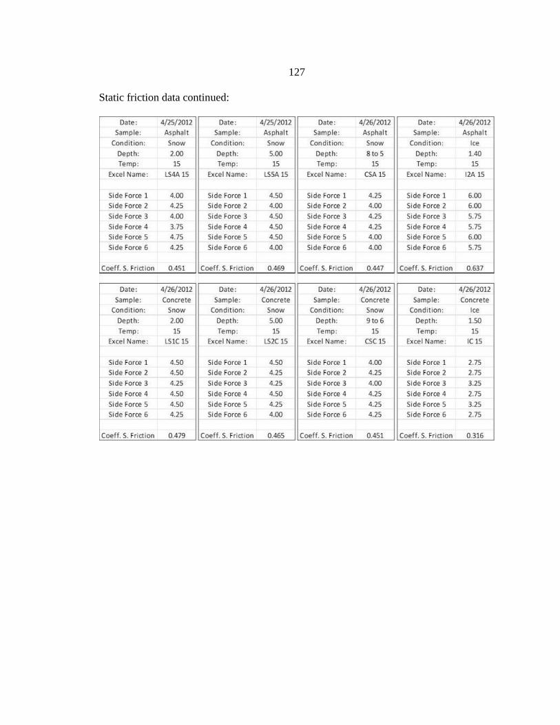
127
Static friction data continued:

128
The following shows the repeatability of measuring 23mL, applying that to the proctor
depth test mold, and the corresponding DSC-111 depth readings.

129
The following shows a small portion of the overall depth calibration spread sheet with the
actual water depth predicted (black and blue), measured (red), and all alphas.