waves - university of oxfordwilkinsong/wavemotion_waves...stretched string and the wave equation 3....

Waves

1

1. N coupled oscillators – towards the continuous limit 2. Stretched string and the wave equation 3. The d’Alembert solution 4. Sinusoidal waves, wave characteristics and notation

Waves 1

2

12

1pp

0 1 2 3 1p 1pp 1NN

l

y

x

T

T

N coupled oscillators Consider flexible elastic string to which are attached N particles of mass m, each a distance l apart. The string is fixed at each end. Small transverse displacements are applied → transverse oscillations

iii tansin 12/1cos2

ii All angles small, i.e. and

No significant horizontal force, since . But vertically: 0coscos 1 pp TT

)()(

sinsin

11

1

pppp

pppp

yyl

Tyy

l

T

TTymF

0)(2 11

2

0

2

0 pppp yyyy

mlT /2

0 with 3

N coupled oscillators: special cases

02

02

1

2

02

2

02

2

2

01

2

01

yyy

yyy

01

2

01 qq 03 2

2

02 qq

0 03

02 1

2

01 yy 02

N=1

N=2

First consider the special cases N=1 and N=2

)(2

1211 yyq )(

2

1212 yyq Try and

mlT /2

0

4

N coupled oscillators: general case

0)(2 11

2

0

2

0 pppp yyyy We have

Consider trial solution tAy pp cos

(For simplicity we’re not allowing for additional phase offset , e.g. . Equivalent to imposing all masses start at rest ) )cos( ppp tAy

0)()2( 11

2

0

2

0

2 ppp AAA ),...,2,1( Np

Substituting in trial solution gives N equations:

2

0

2

0

211 2

p

pp

A

AA(For p=0 and p=N+1 we know Ap=0 )

Since ω is same for all masses we see RHS can’t depend on p & so nor can LHS

5

N coupled oscillators: general case

Look for form for Ap that p

pp

A

AA 11 1. Leaves independent of p 2. Satisfies Ap=0 for p=0 and N+1

Try so pCAp sin

cossin2

)1sin()1sin(11

pC

ppCAA pp

cos211

p

pp

A

AAwhich satisfies 1.

,...)3,2,1()1( nnN and requiring satisfies 2.

1sin

N

pnCAp

1cos2

22

0

2

0

211

N

n

A

AA

p

pp

1cos12

2

0

2

N

n

)1(2sin2 0

N

n

6

12

1pp

0 1 2 3 1p 1pp 1NN

l

y

x

T

T

)cos(1

sin)( nnnpn tN

pnCty

)1(2sin2 0

N

nn

Displacement for mass p when oscillating in mode n and angular frequency:

(note we have smuggled back in the phase offset φn)

mlT /0

Although the value of n can go beyond N, this just generates duplicate solutions, i.e. there are N normal modes in total.

N coupled oscillators: the solution

7

N coupled oscillators: modes for N=5

n=3

n=1

n=4

n=2

n=5

Look at each mode for N=5, with snapshot taken at t=0

Note how the displacement of every particle falls on a sine curve!

8

N coupled oscillators: N very large

)1(2sin2

N

n

ml

Tn

Let’s consider string-mass system of fixed length L and mass M, i.e.

lNL )1( NmM lm /and define linear density

We’ll focus on case N very large, which is starting to approximate to real string

n is small

Look first at mode numbers which are low in value compared with N

lN

n

lm

Tn

)1(2/2

T

Lnn

so normal frequencies are integer multiples of a lowest frequency ω1

T

L1

9

N coupled oscillators: N very large n is small

T

Lnn We have , what about displacements?

)cos(1

sin)( tN

pnCty nnpn

General result . Now separation between

particles becomes smaller & we approach a continuous variable . plx

)cos(sin),( tL

xnCtxy nnn

i.e. string gets closer and closer to lying on a sine curve

10

N coupled oscillators: N very large n =N

0

0

2

)1(2sin2

N

nN

1)sin(

)sin(

1

)1(sin

1sin

1

p

p

N

Np

N

pN

A

A

p

p

Look first at frequency of highest mode

Now consider displacement of successive masses

So we have something like this

Realising this, we see eqn of motion for a given mass is from which we can recover the result l

yTym

22

02 N11

System of springs and N masses: longitudinal oscillations

k

pu

m kkkk m mm

0)(2

)()(

11

2

0

2

0

11

pppp

ppppp

uuuu

uukuukum

mk /2

0 with

Let up be displacement from equilibrium position of mass p

Equations of motion have same form as for masses on string → same solutions!

12

Stretched string

Consider a segment of string of linear density ρ stretched under tension T

x

T

y

xx

T

cos)cos(

sin)sin(

TTF

TTF

x

y

since δθ small 0

x

y

F

TF Tax y )(and so

,small

13

Stretched string

x

T

y

xx

T

Tax y )( T

t

yx

2

2

)(

Note the partial double derivative, rather than

which implies . y depends on both x and t.

This and much of what follows will concern partial differential equations.

y 2

2

d

d

t

y

i.e.

,and since small and xx

2sec1sec

x

y

tan

2

22sec

x

y

x

Now so

2

2

x

y

x

2

2

2

2

t

y

Tx

y

Therefore and so

14

Stretched String and the wave equation

2

2

2

2

t

y

Tx

y

We have performed a similar analysis to the N oscillating masses on a string.

- Then we had N coordinates, yp(t), p=1...N. - Now we have y(x,t), x which are continuous variables

Have obtained

Now (ρ/T) has dimensions of 1/speed2 and indeed we will see that these parameters do define the velocity of travelling waves on the string.

2

2

22

2 1

t

y

cx

y

Tc

This is the wave equation

15

Jean-Baptiste le Rond d’Alembert

• 1717-1783 • Lived in Paris • Mathematician and physicist • Also a music theorist and co-editor with Diderot of a famous encyclopaedia

16

d’Alembert solution of wave equation

2

22

2

2

2

2

2v

y

vu

y

u

y

v

y

u

y

vx

v

ux

u

x

v

v

y

x

u

u

y

xx

y

cv

yc

u

yt

v

v

y

t

u

u

y

t

y

)(11

v

y

u

yx

v

v

y

x

u

u

y

x

y

2

22

2

22

2

2

2v

y

vu

y

u

yc

v

yc

u

yc

vt

v

ut

u

t

v

v

y

t

u

u

y

tt

y

2

2

22

2 1

t

y

cx

y

ctxv

ctxu

y is a function of x and t. Define new variables so that y is now a function of u and v

Chain rule to get first derivatives

and then second derivatives

17

d’Alembert solution of wave equation

2

2

22

2 1

t

y

cx

y

ctxv

ctxu

y is a function of x and t. Define new variables so that y is now a function of u and v

02

vu

y

)()(),( vgufvuy

)()(),( ctxgctxftxy

Here f and g are any functions of (x-ct) and (x+ct). They are determined by initial conditions.

So general solution of wave equation is

18

Interpretation of d’Alembert solution

Lets focus on f(x-ct) part of solution

2

2

22

2 1

t

y

cx

y

)()(),( ctxgctxftxy

is general solution of

At time t=t1:

)(),( ctxftxy

)(),( 11 ctxftxy

At time t=t2:

))](([

)(

)(),(

112

121

22

ctttcxf

ctctctxf

ctxftxy

i.e. displacement at time t2 and position x = displacement at time t1 a distance c(t2-t1) to the left of x

solution describes wave travelling to right with speed c 19


)0,0(y

y

x

),0( ty

y

x

tc

)(),( ctxftxy

Focus on x=0 and consider situations at t=0 and t=Δt

Wave moves to right with speed c

20


)0,0(y

y

x

),0( ty

y

x

tc

)(),( ctxgtxy

Focus on x=0 and consider situations at t=0 and t=Δt

Wave moves to left with speed c

21

d’Alembert’s solution with boundary conditions

)()(),( ctxgctxftxy functions f and g are determined by initial conditions

Suppose at time t=0, the wave has initial displacement U(x) and velocity V(x)

)()()()0,( xgxfxUxy

)(')('

)(d

d)(

)(d

d)()(

)0,(

xcgxcf

ctx

g

t

ctx

ctx

f

t

ctxxV

t

xy

x

b

xxVc

xgxf d)(1

)()(

x

b

xxVc

xUxg d)(2

1)(

2

1)(

x

b

xxVc

xUxf d)(2

1)(

2

1)(

Integrating (2) gives

and combining with (1) yields

(1)

(2)

22


)()(),( ctxgctxftxy functions f and g are determined by initial conditions

Suppose at time t=0, the wave has initial displacement U(x) and velocity V(x)

x

b

xxVc

xUxg d)(2

1)(

2

1)(

x

b

xxVc

xUxf d)(2

1)(

2

1)(

ctx

ctx

ctx

b

ctx

b

xxVc

ctxUctxU

xxVxxVc

ctxUctxUtxy

d)(2

1)()(

2

1

d)(d)(2

1)()(

2

1),(

23


y

x

y

x

y

x

y

x

Example: rectangular wave of length 2a released from rest

)()(2

1),( ctxUctxUtxy

)(xU

0t cat 2/

cat / cat 2/3

24

a a

a

a

aa

a

a

Sinusoidal waves

)()(),( ctxgctxftxy

A very common functional dependence for f and g...

...is sinusoidal. In this case it is usual to write:

)cos()cos(),( tkxBtkxAtxy

or Asin(kx-ωt) ... etc (choice doesn’t matter, unless we are comparing one wave with another and then relative phases become important)

with k and ω (and A and B) constants

• speed of wave

• frequency

where ω is angular frequency

• wavelength where k is the wave-number (or wave-vector if also used to indicate direction of wave)

kc /

2//1 Tf

k/2

25

Notation choices

)cos(),( tkxAtxy Sinusoidal solution (writing here, for compactness, only the forward-going solution)

Using the relationships between k,ω, λ & c this can be expressed in many forms

)](cos[),( ctxkAtxy

Also note that sometimes it is convenient to write

Changes nothing (for cosine, trivially so, & practically not even for sine function, as overall sign can be absorbed in constant) & still describes forward-going wave.

)cos(),( kxtAtxy

A very frequent approach is to use complex notation (we already made use of this when analysing normal modes, and you will have seen it in circuit analysis)

)](exp[Re),( tkxiAtxy

or if its important to pick out sine function. Note that often the ‘Re’ or ‘Im’ is implicit, and it gets omitted in discussion.

)](exp[Im),( tkxiAtxy

26

Phase differences

)cos(),(1 tkxAtxy

Often important to specify phase shifts. Only meaningful to do so when we are comparing one wave to another.

)cos(),(2 tkxAtxy

In this example wave 2 leads wave 1 by π/2, i.e. φ=-π/2

Can be expressed with complex notation

ωt

wave 1 wave 2

π/2

kx=0

)](exp[Re),(2 tkxiAtxy

)](exp[Re),(2 tkxiAtxy )exp(|| iAA

Nicer still to subsume phase into amplitude

with

27

1. Standing waves 2. Transverse waves in nature: electromagnetic radiation 3. Polarisation 4. Dispersion 5. Information transfer and wave packets 6. Group velocity

Waves 2

28

Standing waves Consider a string with 2 waves of equal amplitude moving in opposite directions

tkxA

tkxAtkxAtxy

cossin2

)sin()sin(),(

i.e. has factorised into space and time-dependent parts. This means every point on string is moving with a certain time-dependence (cosωt), but the amplitude of the motion is a function of the distance from the end of the string

T

txAtxy

2cos

2sin2),(

or, if you prefer

t=0

t=δt

λ 2λ x

An example – a string on two which two wavelengths are excited

Stationary points are the nodes – occur every λ/2. Between these are the antinodes.

29

Standing waves

t=0

t=δt

λ 2λ x

T

txAtxy

2cos

2sin2),(

Boundary condition that each end of a fixed string must be a node...

0),(),0( tLyty

...means that only certain discrete frequencies – the modes – are available. These modes are multiples of the basic mode, which is the fundamental .

n

Ln

2

T

Lnn

Wavelengths must ‘fit’, hence wavelength of mode n

Recalling /Tc

gives angular frequency of mode n

with

We already obtained this result when discussing ‘lumpy string’ with N large!

x=L x=0

mode 4

30

Standing waves – violin string

E string of a violin is to be tuned to a frequency of 640 Hz. Its length and mass (from bridge to end) are 33 cm and 0.125 g respectively.

What tension is required?

Fundamental given by

T

Lf

2

1

2)2( LfT

Above parameters give 68 N

31

Transverse waves in nature: EM radiation

The most important example of waves in nature is electromagnetic radiation, i.e. light etc. This will be properly covered in EM lectures. Here is just a taster.

James Clerk Maxwell 1831-1879

Maxwell’s equations in free space for electric field E, and magnetic inductance B

)4()2(

)3(0.)1(0

00tt

EB

BE

BE

ε0 = permittivity of free space = 8.854 x 10-12 F/m μ0 = permeability of free space = 4π x 10-7 Hm-1

B

BBB2

2 )()(

2

2

0000

)()(

tt

BEB

Vector calculus identity plus (3): Making use of (4) and (2):

32


2

2

00

2

t

BB

Maxwell’s equations in free space yield:

which is the wave equation with → the speed of light! 18

00

ms10997.21

c

(equivalent expression is obtainable for E)

Let’s then consider a wave travelling in z-direction (using complex notation):

)](exp[)(

)](exp[

tkziBBB

tkzi

zyx

kji

BB 0 (that we take real part is implicit)

0 B 0

z

B

y

B

x

B zyx 0zkBFrom Maxwell , that is and so

B field has no component in direction of propagation - any oscillation is in transverse plane. Same argument follows for E field → wave is transverse!

Maxwell’s equations also imply that E and B vectors are transverse to each other (not shown here – exercise for the student!)

33


B-field

E-field

EM waves in vacuum: both E and B vectors oscillate transverse to the direction of propagation and, in phase, transverse to each other

34

Transverse vs longitudinal waves

For coupled oscillators we considered both transverse and longitudinal excitations. The same is true here – can certainly have longitudinal waves

Some systems support only transverse waves, some only longitudinal, some both

• Transverse only: stretched string, EM waves in vacuum...

• Longitudinal only: sound waves in air – this because air has no elastic resistance to change in shape, only to change in density

• Both: stretched spring, crystal...

Transverse waves have an important attribute not available to longitudinal waves:

POLARISATION

35

Polarisation Transverse vibrations can be in one of two directions (or both) orthogonal to the direction of wave propagation. We talk of two different directions of polarisation.

(It can even be that wave velocities are different for the two polarisation states, due to e.g. the different interatomic spacings in a crystal.)

Some possibilites for polarisation of E vector in EM wave travelling in z-direction:

x

y

0

)cos(0

y

x

E

tkzEE

)cos(

0

0 tkzEE

E

y

x

x

y

)cos(2/

)cos(2/

0

0

tkzEE

tkzEE

y

x

x

y

)sin(

)cos(

0

0

tkzEE

tkzEE

y

x

x

y

E

E

E E

plane of oscillation

linear linear

linear

circular – rotates with time

36

Dispersion /Tc For our stretched string we found that the wave velocity is,

i.e. depends only on properties of string and has no dependence on frequency (or wavelength) of wave. But this is an idealised system!

For most systems the velocity of a wave does have a dependence on ω and λ

→DISPERSION

One well known example is light in a prism. Light in a medium m with refractive index n Has a velocity cm, where . But the refractive index, and hence wave velocity, varies with wavelength. Hence light is bent at different angles by prism according to wavelength.

nccm /

37

Dispersion – lumpy string revisited The stretched string has an idealised mass / unit length. But earlier we analysed normal modes of the lumpy string. We found:

)1(2sin2 0

N

nn

mLT /0

and ; also we have nLn /2

Recall normal modes for N=5:

Look at behaviour of ωn vs k (for n=1...N), recalling that wave speed=ω/k

Lnk nn //2

with

L n=3

n=2 n=1

n=4

n=5

38

Dispersion curve for lumpy string

For a lumpy string with N=100 masses (other properties arbitrary) calculate ω and k for each normal mode

Note also that there is a ‘cut-off’ frequency – a maximum frequency above which it is not possible to excite system/transmit waves – this is a property often found in a dispersive system.

This is not linear! Velocity of wave corresponding to each mode depends on ω (or k). This is dispersion.

ω/ω

0

kn

increasing n→

Saturates towards cut-off angular frequency of 2ω0

39

Information transfer & wave packets To transmit information it is necessary to modulate a wave. Consider the simplest case of turning a wave on and then off:

For a certain range of (kx-ωt) this signal has displacement y=Asin(kx-ωt), outside this range the displacement y=0. This is not a single wave, for which y=Asin(kx-ωt) would apply for all (kx-ωt)! It is in fact a wave packet.

A wave packet can be formed by summing together (a possibly infinite number of) waves of different frequencies – this is a Fourier series (2nd year topic)

N

n

nnn txkDtxy1

)cos(),(

40

Modulation

41

A pure sine wave carries no information – to encode information for radio transmission need to modulate the wave. General principle as follows:

Signal, typically characterised by low frequency variation

(e.g. voice: a few 100 Hz -1kHz)

Carrier wave High frequency

(e.g. ~ MHz)

Modulated signal, which is transmitted, received and then de-modulated

Carrier signal is modulated

Various options exist for the modulation strategy

Modulation strategies

42

Pulse modulation

Simply turn sine wave off and on, e.g. morse code

Amplitude modulation

Modulate amplitude, e.g. (Offset + signal(t) ) x sin [2π fcarrier t]

Frequency modulation

Encode information in modulation of frequency (also phase modulation)

Wave packets – a toy example

txkkAy

txkkAy

)()(sin

)()(sin

2

1

Sum together two waves which differ by 2δω and 2δk in angular frequency and wave-number, respectively:

to give )sin()cos(221 tkxtxkAyyy

Not exactly a packet, more an infinite series of sausages – would need an infinite number of input waves to make a discrete wave packet

y1

y2

y

43

Group velocity The velocity of the wave packet is known as the group velocity. In almost all cases this is the velocity at which information is transmitted.

In a dispersive medium the group velocity is not the same as the velocity of the individual waves, which is known as the phase velocity (& in a dispersive medium the phase velocity, ω/k, varies with frequency & wavelength)

y

)sin()cos(221 tkxtxkAyyy

Consider our toy example:

Describes envelope – so envelope moves with velocity and indeed k

Group velocity while phase velocity k

vgd

d

kvp

44

Cartoon of wave packet (1/7)

A travelling wave packet. The marks the top of the wave packet which moves with the group velocity. The indicates a component wave crest which enters the packet, moves through it, and leaves, with the phase velocity.

45



46



47



48



49



50



51

kvg

d

dWe have already stated

but so kvpdk

dvkvv

p

pg

also, since /2k

d

dvvv

p

pg

or if considering light, & a medium with refractive index n, we have ncvp /

d

dn

nn

cvg 1

Observe that ! ncvg /

Different expressions for the group velocity

52

Dispersion and the spreading of the wave packet

Another consequence of dispersion is that a wave-packet will not retain its shape perfectly, but will spread out. Can have consequences for signal detection

53

Group and phase velocities for lumpy string

Calculate phase and group velocity for the lumpy string with N=100

ω/ω

0

kn ω/ω0

Ratio of vg to vp V

g /

v p

Vel

oci

ty

vg

vp

Phase and group velocity ~ the same at first, but vg→0 as ω→2ω0 (cut-off)

Dispersion curve

54

Waves in deep water Waves in water with λ > 2 cm (below which surface tension effects are important), but still small compared to water depth, have a dispersion relation

i.e. driven by gravity, hence often called gravity waves - ocean swell

)(gk

pg vkk

g

dk

dv

2

1

2

1

2

1

So group velocity is half that of phase velocity

55

Estimating how far away a sea storm is

)(gkDispersion relation means that and so waves of longer wavelengths travel more quickly.

)2/()( gvp

2/1)/2( gvp

// 00 LtvLtt p )(/2 0ttgL

LgttgLdt

d

2/)(/2 22

0

Storm Measure interval between successive wave crests a long way (L) distant

L

e.g. if L=1000 km and τ=10 s then -dτ/dt= 1.2 x 10-4 (0.6 s / hour)

So if measure period and rate of decrease in period can obtain L !

Period of wave: Time of arrival of wave crests: Eliminate λ:

Hence

56

1. Energy stored in a mechanical wave 2. Wave equation revisited - separation of variables 3. Wave on string with fixed ends 4. Waves at boundaries 5. Impedance 6. Other examples: - Lossless transmission line - Longitudinal waves in a bar - Acoustic waves

Waves 3

57

Energy stored in a mechanical wave

A vibrating string must carry energy – but how much? Lets calculate the kinetic energy density (i.e. KE / unit length) and potential energy density

x x + dx

y

y+dy ds Consider small segment of string of linear

density ρ between x and x+dx displaced in the y direction. As usual, assume displacement is small

2

2

2

1)(

2

1

t

ydxudxK y

2

2

1

d

ddensity KE

t

y

x

K

Kinetic energy,

58


x x + dx

y

y+dy ds

Potential energy, U, is work done by deformation

)dd( xsTU

...2

11

1dd

2

2/12

x

ydx

x

yxs

xx

yTU d

2

12

2

2

1

d

ddensity PE

x

yT

x

U

59


2

2

1

d

ddensity KE

t

y

x

K

2

2

1

d

ddensity PE

x

yT

x

U

)(' zfx

y

)(' zvf

t

y

22

2

)]('[2

1

2

1

d

d

zfv

t

y

x

K

2

2

)]('[2

1

2

1

zfT

x

yT

x

U

We have shown

)()(),( zfvtxftxy and we know solutions take form , say

therefore

and so

)/( Tv These are equal since - one manifestation of the Virial Theorem.

60

Energy stored in a mechanical wave Let’s explicitly calculate KE and PE for a sinusoidal wave )sin( tkxAy

Evaluate these quantities over an integer number of wavelengths

22

1

d)](2cos[12

1

2

1

d)(cos2

1

22

22

222

nA

xtkxA

xtkxAK

nx

x

nx

x

22

1

d)](2cos[12

1

2

1

d)(cos2

1

22

22

222

nkTA

xtkxkTA

xtkxkATU

nx

x

nx

x

kTv /)/( 22 Tk Now and so these expressions are equal

Thus total energy / unit length 22

2

1A

Moreover, we can evaluate energy flow/unit time (= power to generate wave)

P = (energy / wavelength) x (distance travelled / time)

22222

2

1

2

1

2

1kAT

kATkvAP

61

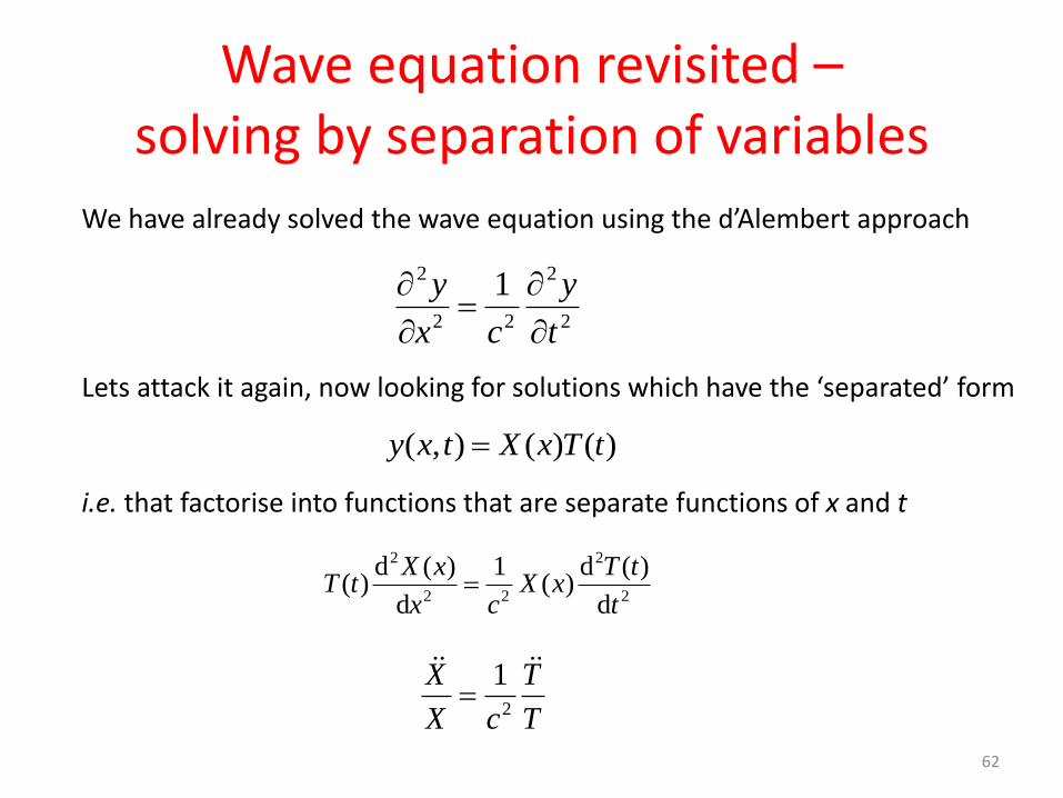
Wave equation revisited – solving by separation of variables

2

2

22

2 1

t

y

cx

y

We have already solved the wave equation using the d’Alembert approach

Lets attack it again, now looking for solutions which have the ‘separated’ form

)()(),( tTxXtxy

i.e. that factorise into functions that are separate functions of x and t

2

2

22

2

d

)(d)(

1

d

)(d)(

t

tTxX

cx

xXtT

T

T

cX

X 2

1

62


T

T

cX

X 2

1)()(),( tTxXtxy

Separated solution to wave equation e.g.

gives

Can only be satisfied if both sides equal a constant:

CT

T

cX

X

2

1

the separation constant

Lets consider first the case when C is negative. We write C=-k2

XkX 2 TckT 2)(

These are SHM equations, so we can write

kxBkxAxX sincos)( cktEcktDtT sincos)( with A,B,D and E constants defined by initial conditions

so e.g. in case B=0 and D=0 we have

tkxFtxy sincos),(

a form we have seen before, when manipulating d’Alembert solution

with ω=ck (and F=AE...)

63


CT

T

cX

X

2

1

C negative already considered. Here are some other possibilities:

• C is positive = k2

))((),( kctkctkxkx EeDeBeAetxy

))((),( EtDBxAtxy

• C = 0

Still others exist (e.g. C is complex). Which of solutions is relevant depends on the physical situation. Here we are usually interested in C is negative, since then we get oscillations! But even then many possibilities exists (=different values of k), and we will often get a linear superposition of these.

Wave equation with separated variables:

64

Wave on string with fixed ends

0x Lx

Consider a string with fixed ends, initially at rest, given an initial displacement and released. Describe its subsequent motion.

Know from separation of variables that a solution to wave equation is

)sincos)(sincos(),( kctDkctCkxBkxAtxy

and we also have four boundary conditions. Three of them are as follows:

1. String initially at rest, i.e. for all x

2. y(0,t)=0

3. y(L,t)=0 where n any integer. This is the eigenvalue eqn. and discretises k. Each value of n corresponds to a normal mode. It is clear that for this continuous system n can go to infinity...

0/ ty 0D

0 A

nkL

65

Wave on string with fixed ends

1

cossin),(n

nL

ctn

L

xnFtxy

Therefore, by the principle of superposition, the solution is:

i.e. sum of all possible solutions with coefficients Fn given by initial displacement, which is the boundary condition we have not yet invoked

1

)(sin)0,(n

n xhL

xnFxy

where h(x) is pattern of initial displacement

Simplest case is when h(x) is just a normal mode, e.g.

L

xxh

5sin)( 5when 0 and15 nFF n

L

ct

L

xtxy

5cos

5sin),(

66

Wave on string with fixed ends Consider a more complicated situation when h(x) is not a single normal mode

L

x

L

xxh

2sin

2

1sin)(

L

ct

L

x

L

ct

L

xtxy

2cos

2sin

2

1cossin),(

Then it is clear F1=1, F2=0.5 and Fn=0 when n ≠ 1 or 2, so

In contrast to case with just a single normal mode the subsequent motion is not equal to initial displacement x varying amplitude. Since the shorter waves are faster the shape of the wave varies during oscillation.

0x Lx

Even if the initial displacement looks like this (i.e. plucked string), it can be expressed as sum of normal modes!

→ Fourier series (year 2) 67

Wave on string with fixed ends: energies of normal modes

L

ctn

L

xnFtxy nn

cossin),(

Normal mode n for our problem, with given boundary conditions:

Calculate kinetic energy, Kn, and potential energy, Un, for each mode

xt

yK

L

nn d

2

1

0

2

x

x

yTU

L

nn d

2

1

0

2

L

ctn

L

cnF

xL

xn

L

ctn

L

cnFK

n

L

nn

22

0

22

2

2

sin4

)(

dsinsin2

1

L

ctn

L

nFT

xL

xn

L

ctn

L

nTFU

n

L

nn

22

0

22

2

2

cos4

)(

dcoscos2

1

Since we have )/( Tc 44

222

2

2

nnn

nnnn

LFE

L

nc

LFUKE

68

Wave on string with fixed ends: energies of system

Now let’s calculate energy of system, with arbitrary initial displacement

1

cossin),(n

nL

ctn

L

xnFtxy

1 11

terms-crossn mn

nEE

This is simple extension of exercise for individual normal modes, But with additional terms

mnxL

xm

L

xnL

withdsinsin0

but cross-terms all include factors of the type

which are zero!

1n

nEE i.e. total energy is sum of energies of normal modes

69

Waves at boundaries What happens for a wave propagating on a string when it encounters a boundary across which the string characteristics change, e.g. change of linear density ρ1,2 ?

Since the tension, T, is constant across boundary, it follows phase velocities change

2,12,1 / Tc

x=0

ρ1

ρ2

We must allow for the possibility of three waves:

Incident wave

Reflected wave Transmitted wave

x→

70

Waves at boundaries

Let’s write down the three waves

x=0

ρ1

ρ2

x→

)sin( 1xktA

)sin(' 1xktA

)sin('' 2xktA

Incident

Reflected

Transmitted

(we have switched to writing sin(ωt-kx) rather than sin(kx-ωt), as this notation is usual for these problems. But this does not affect anything.)

• We assume same angular frequency, ω, on both strings. This is required by boundary conditions (see later). but wavelength, and hence wave number, medium-dependent

• The relative values of A, A’ and A’’ are to be determined

Note:

Observe the + sign in argument for left-going wave

71

Boundary conditions

x=0

ρ1

ρ2

x→

• String is continuous • Vertical component of force on left of boundary must be balanced by vertical component on right

),0(),0( 21 tyty

),0(),0( 21 tx

yt

x

y

Two boundary conditions:

)sin(')sin(),( 111 xktAxktAtxy

)sin(''),( 22 xktAtxy

Here:

net wave to left of boundary

wave to right of boundary

72

Applying boundary conditions

String continuous (1) → Balanced vertical tension (2) →

'''

sin''sin'sin

AAA

tAtAtA

'')'(

cos''cos'cos

21

211

AkAAk

tAktAktAk

21

21'

kk

kk

A

Ar

21

12''

kk

k

A

At

Solve to obtain amplitude reflection and transmission coefficients

)1(),0(),0( 21 tyty

)2(),0(),0( 21 tx

yt

x

y

)sin('

)sin(),(

1

11

xktA

xktAtxy

)sin(''),( 22 xktAtxy

Applying with

73

Applying boundary conditions

We have and 21

21'

kk

kk

A

Ar

21

12''

kk

k

A

At

Lets consider some specific cases:

• k1=k2 then r=0, t=1 – no reflection and full transmission

• k1<k2 then A’ is negative and can write reflected wave

• k1>k2 then A’ is positive • ρ2→ hence

Full reflection (with phase change) and no wave in second string

)sin(|'|)sin(|'| 11 xktAxktA

i.e. there is a phase change at a rare-dense boundary (since ) 2121,// kkTkc

2k 1'

A

Ar

74

Power flow at a boundary

We have and 21

21'

kk

kk

A

Ar

21

12''

kk

k

A

At

2

2

1kATP and earlier we showed that

2

21

21

2

1

2

1

2

1

'2

1

kk

kk

ATk

ATk

Rr

2

21

21

2

1

2

2

)(

4

2

1

''2

1

kk

kk

ATk

ATk

Rt

1)(

)4()2(2

21

2121

2

2

2

1

kk

kkkkkkRR tr

So ratios of reflected to incident power, Rr, and transmitted to incident power, Rt, are given by

and so , as expected

75

Reflection from a mass at the boundary

x=0

ρ1

ρ2

x→

M

Consider situation where a finite point mass, M, is fixed at the boundary between two semi-infinite strings of density ρ1 and ρ2

Solve as before, but in this case one of the boundary conditions changes

Sum of forces at boundary act on mass and generates transverse acceleration

),0(),0(),0(),0(2

2

2

2

1

2

21 tt

yMt

t

yMt

x

yTt

x

yT

Other boundary condition (system continuous, so ) unchanged ),0(),0( 21 tyty

76


x=0

ρ1

ρ2

x→

M

Here, with 2nd derivatives involved, it’s convenient to use exponential notation

)](exp[')](exp[Re),( 111 xktiAxktiAtxy

)](exp[''Re),( 22 xktiAtxy

System continuous → , as before ''' AAA

New condition → '')'(''' 22

211 MAAAMTAikTAikTAik

'')/()'( 2

21 ATMikAAik

77


''' AAA We have and '')/()'( 2

21 ATMikAAik

)exp()(

)('2

21

2

21

iR

MiTkk

MiTkk

A

Ar

)exp()(

2''2

21

1

iTMiTkk

Tk

A

At

From these can show

Here θ (φ) is phase shift of reflected (transmitted) wave w.r.t. incident wave.

)cos()cos(),(

)](exp[')](exp[Re),(

111

111

xktRAxktAtxy

xktiAxktiAtxy

)cos(),(

)](exp[''Re),(

22

22

xktTAtxy

xktiAtxy

Here R and T are real numbers

78


)exp()(

)('2

21

2

21

iR

MiTkk

MiTkk

A

Ar

)exp(

)(

2''2

21

1

iTMiTkk

Tk

A

At

2/1

2422

21

2422

21

)(

)(

MTkk

MTkkR

Tkk

M

Tkk

M

)(tan

)(tan

21

21

21

21

2/1

2422

21

22

1

)(

4

MTkk

TkT

Tkk

M

)(tan

21

21

For completeness – we have:

and so

once more note , i.e. energy conserved 1|||| 2

1

222

1

22 Tk

kRt

k

kr

79


Consider special case where second string has zero density: ρ2=0. Then k2=0 and it as if we are just terminating the first string with the mass.

1

2/1

2422

1

2422

1

MTk

MTkR

Tk

M

Tk

M

Tk

M

1

21

1

21

1

21

tan2

tantan

→0 if M is small

→π if M is large

Total reflection

80

Impedance Familiar with concept of electrical impedance from circuit theory

= a measure of opposition to a time varying electric current

IZV

different components have different impedances, some frequency dependent

RZR

CiZC /

LiZL

resistor

capacitor

inductor

For structures along which electromagnetic waves propagate, i.e. transmission lines, even free space, talk of characteristic impedance

But concept of impedance and characteristic impedance can be used in other wave-carrying systems. Here is an (admittedly) woolly definition:

Impedance is ratio of ‘push variable’ (i.e. voltage or pressure) to a ‘flow variable’ (i.e. current or particle velocity)

81

Impedance & waves on string

The characteristic impedance Z is defined as the applied driving force acting in the y-direction divided by the velocity of the string in the y-direction

For transverse waves on a string:

t

yx

yT

v

FZ

y

y

so with

)sin(),( tkxAtxy )(

T

c

TTkZ

Also, can take reflection and transmission coefficients from ‘mass at a boundary’ problem and write these in terms of impedances

)(

)(

)(

)('

21

21

2

21

2

21

M

M

ZZZ

ZZZ

MiTkk

MiTkk

A

Ar

)(

2

)(

2''

21

1

2

21

1

MZZZ

Z

MiTkk

Tk

A

At

Here we have the characteristic impedances

which are ‘resistive’, and an impedance for the mass itself of

which is ‘inductive’

/2,12,1 TkZ

MiZM

82

Other important examples

• Transmission lines

• Longitudinal elastic waves

- Oscillations in a solid bar

- Acoustic waves in gas

83

Lossless transmission lines

I II

V VV

x xx

Consider a system made of inductors and capacitors, and then let it become continuous so that we now speak of inductance / unit length L’ & capacitance / unit length C’ (e.g. coaxial cable). Let it have zero resistance (‘lossless’).

Self-inductance of δx = L’δx → voltage change Capacitance of δx = C’δx → voltage change

t

IL

x

Vt

IxLV

'

)'(

x

I

t

VC

xCQV

'

)'/(

84

Lossless transmission lines

I II

V VV

x xx

)1('t

IL

x

V

)2('

x

I

t

VC

these are the telegraph equations

We have shown

)2(

xand)1(

t 2

2

2

2

''t

ICL

x

I

)1(

xand)2(

t 2

2

2

2

''t

VCL

x

V

Wave equation!

So waves of form e.g.

can travel down line with

)sin(

)sin(

0

0

kxtII

kxtVV

''/1 LCc

Characteristic impedance of transmission line

I II

V VV

x xx

t

IL

x

V

'

)sin(

)sin(

0

0

kxtII

kxtVV

)cos(')cos( 00 kxtILkxtkV

'

''

''

1'

0

0

C

LL

LCL

kI

VZ

(+ve for forward travelling wave)

We have and

Characteristic impedance

86

Reflection at a terminated line

Consider how wave reflects for transmission line of characteristic impedance Z0 terminated at x=0 by an impedance of ZT

x→

x=0 incident, V0=A

reflected, V0=A’

ZT

Z0

])[exp('])[exp(),(

])[exp('])[exp(),(

0 kxtiAkxtiAtxIZ

kxtiAkxtiAtxV

We have:

Now at x=0 the ratio V/I must = the terminating impedance! TZtI

tV

),0(

),0(

'

'

0 AA

AA

Z

ZT

0

0'

ZZ

ZZ

A

Ar

T

T

Hence, so reflection coefficient

• ZT→0 then r→-1: full reflection with phase shift

• ZT=Z0 then r→0 : no reflection – matched impedance; all power transmitted to terminating load

• ZT→ then r→1: full reflection 87

Longitudinal waves in a solid bar

x

x

A

A F FF

direction of wave

x

x

under equilibrium

under disturbance from wave

Consider a solid bar, initially in equilibrium, in which a disturbance perturbs the position and thickness of a slice of material

We denote by F the magnitude of the new stress force stretching the material and δF the excess force accelerating the segment to the right

88

Longitudinal waves in a solid bar

Mass of slice (with density ρ) is given by and acceleration is xA 2

2

t

xY

A

F

x

AYF

Force per unit area on slice is given by Hooke’s law and Young’s modulus of the material, Y

infinitely thin slice

xx

AYF

2

2

So excess force is given by

2

2

2

2

2

2

2

2

)(tYx

xx

AYt

xA

Newton II gives

So velocity of waves is

Yv

Steel has Y=2 x 1011 Nm-2

and ρ= 8000 kg m-3

1skm5 v

89

Acoustic waves Sound waves are longitudinal waves associated with compression of medium.

x

x

A

A pp ppp

p p

direction of sound wave

x

x

under equilibrium

under disturbance from sound wave

Consider a slice of gas, initially at equilibrium, in a tube of cross-sectional area A. Slice is between x and x+δx. A disturbance moves the slice to x+ψ and changes its width to δx+δψ. Pressure has changed from p to p+ψp on LHS of slice, and to p+ψp+δψp on RHS.

90

Acoustic waves

xp

Slice has had its volume changed by a fractional amount (A.δψ)/(A.δx) , and this happens as a result of a pressure change ψp . The relationship is determined by the elasticity of the gas, the bulk modulus κ

px )/1(/ infinitely thin slice

From this we see which will be useful in getting wave eqn. xx

p

2

2

• Mass of slice

• Force on slice in x-dirn

• Acceleration of slice

pA

xA

2

2

t

2

2

2

2

2

2

2

2

tx

xt

Axx

A

These relations and Newton II yield:

91

Acoustic waves

2

2

2

2

tx

We have obtained result , a wave equation describing motion

of a slice of gas at position ψ. One might worry that a ‘slice of gas’ is a rather intangible experimental observable. Instead one can phrase problem in terms of the pressure variations, ψp , which are certainly measurable.

xp

Since then ψp also satisfies wave equation, i.e. 2

2

2

2

tx

pp

t

xZ

)sin(),( kxtAtx

Kv

KKkZ

/vEither way, phase velocity of waves is

Characteristic impedance can be defined by

so for forward-travelling wave

92

Acoustic waves – speed of sound

• Isothermal compression No temperature changes – justifiable if the pressure changes are slow enough to allow tube to exchange heat freely with surroundings.

/vWe have shown that , so we can calculate v if we know κ (and ρ).

To calculate κ it is convenient to use this form of definition:

We also need to specify what else happens to system as p changes. V

pV

• Adiabatic compression Pressure changes occur so rapidly that heat cannot be exchanged from dense to less dense regions. Good approximation to reality.

/pvpV

RT

2V

RT

V

PRTPV

Ideal gas so

constantpV Vp CC /Adiabatic changes in an ideal gas where i.e. the ratio of specific heats at constant p and constant V

V

p

V

P

)/(/ MRTpvp so

i.e. velocity independent of pressure for ideal gas Typical value for air at room temperature ~350 ms-1

93

waves - university of oxfordwilkinsong/wavemotion_waves...stretched string and the wave equation 3....

Documents