wavelets, scattering transforms and convolutional neural ...1170151/fulltext01.pdf · wavelets and...
TRANSCRIPT

Pontus Westermark
Wavelets, Scattering transformsand Convolutional neural networks
Tools for image processing
1

Contents
1 Introduction . . . . . . . . . . . . . . . . . . . . . . . . . . . . . . . . . . . . . . . . . . . . . . . . . . . . . . . . . . . . . . . . . . . . . . . . . . . . . . . . . . . . . . . . . . . . . . . . . . 7
2 Mathematics . . . . . . . . . . . . . . . . . . . . . . . . . . . . . . . . . . . . . . . . . . . . . . . . . . . . . . . . . . . . . . . . . . . . . . . . . . . . . . . . . . . . . . . . . . . . . . . . . 8
2.1 Measure and integration . . . . . . . . . . . . . . . . . . . . . . . . . . . . . . . . . . . . . . . . . . . . . . . . . . . . . . . . . . . . . . . . . . . 8
2.2 Function spaces . . . . . . . . . . . . . . . . . . . . . . . . . . . . . . . . . . . . . . . . . . . . . . . . . . . . . . . . . . . . . . . . . . . . . . . . . . . . . . . . 9
2.2.1 Lp-space . . . . . . . . . . . . . . . . . . . . . . . . . . . . . . . . . . . . . . . . . . . . . . . . . . . . . . . . . . . . . . . . . . . . . . . . . . . . . 9
2.2.2 Continuous function spaces . . . . . . . . . . . . . . . . . . . . . . . . . . . . . . . . . . . . . . . . . . . . 10
2.3 Hilbert spaces . . . . . . . . . . . . . . . . . . . . . . . . . . . . . . . . . . . . . . . . . . . . . . . . . . . . . . . . . . . . . . . . . . . . . . . . . . . . . . . . . 11
2.4 Convolutions . . . . . . . . . . . . . . . . . . . . . . . . . . . . . . . . . . . . . . . . . . . . . . . . . . . . . . . . . . . . . . . . . . . . . . . . . . . . . . . . . . . 11
2.5 Frequency analysis . . . . . . . . . . . . . . . . . . . . . . . . . . . . . . . . . . . . . . . . . . . . . . . . . . . . . . . . . . . . . . . . . . . . . . . . . 14
2.5.1 The L1(R) Fourier transform . . . . . . . . . . . . . . . . . . . . . . . . . . . . . . . . . . . . . . . . . . 14
2.5.2 The L1(R2) Fourier transform . . . . . . . . . . . . . . . . . . . . . . . . . . . . . . . . . . . . . . . . 14
2.5.3 The L1(Rn) Fourier Transform . . . . . . . . . . . . . . . . . . . . . . . . . . . . . . . . . . . . . . . 15
2.5.4 The L2(R) Fourier transform . . . . . . . . . . . . . . . . . . . . . . . . . . . . . . . . . . . . . . . . . . 15
2.5.5 The L2(Rn) Fourier Transform . . . . . . . . . . . . . . . . . . . . . . . . . . . . . . . . . . . . . . . 16
2.5.6 Fourier transform properties . . . . . . . . . . . . . . . . . . . . . . . . . . . . . . . . . . . . . . . . . . . 17
2.5.7 On time and frequency . . . . . . . . . . . . . . . . . . . . . . . . . . . . . . . . . . . . . . . . . . . . . . . . . . . . 19
2.6 Frames . . . . . . . . . . . . . . . . . . . . . . . . . . . . . . . . . . . . . . . . . . . . . . . . . . . . . . . . . . . . . . . . . . . . . . . . . . . . . . . . . . . . . . . . . . . . . 20
2.7 Multi-resolution analysis . . . . . . . . . . . . . . . . . . . . . . . . . . . . . . . . . . . . . . . . . . . . . . . . . . . . . . . . . . . . . . . 21
2.7.1 Properties 1, 2, 3 . . . . . . . . . . . . . . . . . . . . . . . . . . . . . . . . . . . . . . . . . . . . . . . . . . . . . . . . . . . . . . 21
2.7.2 Properties 4, 5 . . . . . . . . . . . . . . . . . . . . . . . . . . . . . . . . . . . . . . . . . . . . . . . . . . . . . . . . . . . . . . . . . . 21
3
2.7.3 Property 6 . . . . . . . . . . . . . . . . . . . . . . . . . . . . . . . . . . . . . . . . . . . . . . . . . . . . . . . . . . . . . . . . . . . . . . . . . 22
2.8 Wavelets . . . . . . . . . . . . . . . . . . . . . . . . . . . . . . . . . . . . . . . . . . . . . . . . . . . . . . . . . . . . . . . . . . . . . . . . . . . . . . . . . . . . . . . . . . 23
2.9 One-dimensional wavelets . . . . . . . . . . . . . . . . . . . . . . . . . . . . . . . . . . . . . . . . . . . . . . . . . . . . . . . . . . . . . 25
2.9.1 Connection to multi-resolution analysis . . . . . . . . . . . . . . . . . . . . . . . . 25
2.9.2 Probability theory for wavelets . . . . . . . . . . . . . . . . . . . . . . . . . . . . . . . . . . . . . . . 26
2.9.3 Time-frequency localization . . . . . . . . . . . . . . . . . . . . . . . . . . . . . . . . . . . . . . . . . . . 27
2.9.4 Convolutions and filters . . . . . . . . . . . . . . . . . . . . . . . . . . . . . . . . . . . . . . . . . . . . . . . . . . 28
2.9.5 Wavelets and filters . . . . . . . . . . . . . . . . . . . . . . . . . . . . . . . . . . . . . . . . . . . . . . . . . . . . . . . . . . 29
2.9.6 Complex Wavelets . . . . . . . . . . . . . . . . . . . . . . . . . . . . . . . . . . . . . . . . . . . . . . . . . . . . . . . . . . . 30
2.10 Two-dimensional wavelets . . . . . . . . . . . . . . . . . . . . . . . . . . . . . . . . . . . . . . . . . . . . . . . . . . . . . . . . . . . . 32
2.10.1 Time-frequency spread . . . . . . . . . . . . . . . . . . . . . . . . . . . . . . . . . . . . . . . . . . . . . . . . . . . . 32
2.10.2 Complex wavelets in two dimensions . . . . . . . . . . . . . . . . . . . . . . . . . . . . 33
2.10.3 Rotations . . . . . . . . . . . . . . . . . . . . . . . . . . . . . . . . . . . . . . . . . . . . . . . . . . . . . . . . . . . . . . . . . . . . . . . . . . 34
2.11 Scattering wavelets . . . . . . . . . . . . . . . . . . . . . . . . . . . . . . . . . . . . . . . . . . . . . . . . . . . . . . . . . . . . . . . . . . . . . . . . . 36
2.11.1 The scattering transform . . . . . . . . . . . . . . . . . . . . . . . . . . . . . . . . . . . . . . . . . . . . . . . . . 40
2.11.2 Properties of the scattering transform . . . . . . . . . . . . . . . . . . . . . . . . . . . . 41
3 Convolutional Networks . . . . . . . . . . . . . . . . . . . . . . . . . . . . . . . . . . . . . . . . . . . . . . . . . . . . . . . . . . . . . . . . . . . . . . . . . . . . 42
3.1 Success of CNNs . . . . . . . . . . . . . . . . . . . . . . . . . . . . . . . . . . . . . . . . . . . . . . . . . . . . . . . . . . . . . . . . . . . . . . . . . . . . 42
3.2 Classical convolutional neural networks . . . . . . . . . . . . . . . . . . . . . . . . . . . . . . . . . . . . . . 43
3.2.1 Structure of a neural node . . . . . . . . . . . . . . . . . . . . . . . . . . . . . . . . . . . . . . . . . . . . . . . 44
3.2.2 The interconnection of nodes . . . . . . . . . . . . . . . . . . . . . . . . . . . . . . . . . . . . . . . . . . 44
3.2.3 Training of CNNs . . . . . . . . . . . . . . . . . . . . . . . . . . . . . . . . . . . . . . . . . . . . . . . . . . . . . . . . . . . . 45
3.2.4 Mathematical challenges . . . . . . . . . . . . . . . . . . . . . . . . . . . . . . . . . . . . . . . . . . . . . . . . . 45
3.3 Scattering Convolution Networks . . . . . . . . . . . . . . . . . . . . . . . . . . . . . . . . . . . . . . . . . . . . . . . . . 46
3.3.1 Hybrid networks . . . . . . . . . . . . . . . . . . . . . . . . . . . . . . . . . . . . . . . . . . . . . . . . . . . . . . . . . . . . . . 46
4
A Multi-resolution analysis of a signal . . . . . . . . . . . . . . . . . . . . . . . . . . . . . . . . . . . . . . . . . . . . . . . . . . . . . . . . 47
B Scattering transforms of signals . . . . . . . . . . . . . . . . . . . . . . . . . . . . . . . . . . . . . . . . . . . . . . . . . . . . . . . . . . . . . . . 48
B.1 Frequency decreasing paths over S3, using ψ , θ . . . . . . . . . . . . . . . . . . . . . . . . . 48
B.2 Frequency decreasing paths over S2, using φ ,θ . . . . . . . . . . . . . . . . . . . . . . . . . . 49
B.3 Constant paths over S3, using ψ,θ . . . . . . . . . . . . . . . . . . . . . . . . . . . . . . . . . . . . . . . . . . . . . . . 50
B.4 Constant paths over S3, using ψ,θ . . . . . . . . . . . . . . . . . . . . . . . . . . . . . . . . . . . . . . . . . . . . . . . 51
B.5 Frequency decreasing path over S5, using ψ,θ . . . . . . . . . . . . . . . . . . . . . . . . . . . 52
B.6 Frequency decreasing path over S5, using ψ2−4 ,θ2−4 . . . . . . . . . . . . . . . . . . 54
4 References . . . . . . . . . . . . . . . . . . . . . . . . . . . . . . . . . . . . . . . . . . . . . . . . . . . . . . . . . . . . . . . . . . . . . . . . . . . . . . . . . . . . . . . . . . . . . . . . . . 55
5

*
6
1. Introduction
Wavelets in their modern form has been studied since the 1980’s [25] andhas found many applications in signal processing such as in compression andimage denoising [18] and the theoretical properties of the waveforms are wellunderstood.
In the most recent years, wavelets have been extended to the domain of ma-chine learning and neural networks, which provides a way to enhance a neuralnetwork with well-defined mathematical properties.
This thesis aims to present all the relevant theory to be able to understandwavelets and how they can be used to define the scattering transform. Thenwe cover the theoretical properties of the scattering transform and how it canbe used in handwritten digit classification.
Moreover, the appendices contain several numerical examples which showboth a multi-resolution analysis of, and how the scattering transform acts on,a signal. All figures in this thesis has been developed by the author.
7
2. Mathematics
2.1 Measure and integration
A lot of important theorems and results that we will use originate from Fourieranalysis and functional analysis, which in turn rely on measure and integrationtheory. Thus we talk briefly about which measure spaces we consider and thenotation that we use for them. However in practice we need mostly ordinarycalculus to work with the integrals that we will encounter. For a completeoverview of measure theory, see [1].
Our measure space will be Rn for some positive integer n, equipped with theassociated Lesbegue measure, here denoted µ . We will allow for any commondenotation of an integral as made precise below.
Notation 1. If f is an integrable function with Rn as its domain, and x =(x1, ...,xn) an n-dimensional vector, we permit ourselves to write its Lesbegueintegral over f ’s entire domain as follows.∫
Rnf dµ =
∫f dµ
=∫
f (x1, ...,xn)dx1...dxn
=∫
f (x)dx.
Similarly, for integration of f over a subset ((a1,b1), ...,(an,bn)) ⊂ Rn wewrite ∫
Af dµ =
∫ b1
a1
...∫ bn
an
f (x1, ...,xn)dx1...dxn
=∫ b1
a1
...∫ bn
an
f (x)dx.
Finally, for integration over (a,b) ⊆ R we write integration over the inverseorientation as
∫ ab f (x)dx =−
∫ ba f (x)dx.
This may seem like a redundant amount of ways to write an integral, but it willaid us later since we will work a lot with concepts based on different types ofintegration.
8
2.2 Function spaces
We begin by giving a suitable definition of an Lp-space, followed by a closerlook at two important special cases, namely L1 and L2 over both R and R2.Then we will briefly look at Ck spaces of continuous and continuously differ-entiable functions, with which we assume that the reader is already familiar.
2.2.1 Lp-space
Definition 1. For a measure space Rn with associated Lesbegue measure µ ,the function space Lp(Rn) is the collection of all functions f : Rn → C suchthat ∫
Rn| f |pdµ < ∞. (2.1)
In this definition, Rn signifies the domain of the functions of Lp(Rn). Thismotivates the following notation.
Notation 2. We write simply Lp when the domain is either obvious in the cur-rent context, or if we wish to speak about something which holds for Lp(Rn)for all n.
Definition 2. To each Lp space, we denote the Lp norm
|| f ||p = (∫| f |pdµ)1/p.
Notation 3. When it is obvious to which Lp space a function f belongs, wewill not write the subscript of the norm, i.e. || f ||p will be written || f ||.
That all Lp spaces are vector spaces is apparent from their respective defini-tions. More information about their properties can be found in [1].
9

Square-integrable, L2(R) and L2(R2)
A function f ∈ L2(R) or f ∈ L2(R) is said to be square-integrable if its squaredmodulus has a finite value. That is, f ∈ L2(R) is square integrable if∫
∞
−∞
| f (t)|2dt < ∞.
Similarly, f ∈ L2(R2) and is also said to be square integrable if∫∞
−∞
∫∞
−∞
| f (x,y)|2dxdy < ∞.
Absolutely integrable, L1(R) and L1(R2)
Analogously, we say that a function f is absolutely integrable if f ∈ L1(R) orif f ∈ L1(R2) and∫
∞
−∞
| f (t)|dt < ∞, or if∫
∞
−∞
∫∞
−∞
| f (x,y)|dxdy < ∞ respectively.
Example 1. The function f (x) = 11+|x| is in L2(R) but not in L1(R), as can be
seen by the following equations.
11+ |x|
=ddx
log(1+ |x|), 1(1+ |x|)2 =
ddx
11+ |x|
.
The integral over R of the former clearly does not converge to a finite valuewhile the latter does.
2.2.2 Continuous function spaces
Definition 3. For k and n positive integers, we define Ck(Rn) as the space ofall k times continuously differentiable functions f : Rn→ C.
Notation 4. In particular, we write C0(Rn) =C(Rn), and if n is obvious fromthe context or if we wish to talk about all k times continuously differentiablefunctions with range C, we simply write Ck =Ck(Rn) or C =C0.
10

2.3 Hilbert spaces
Equipped with the inner product 〈 f ,g〉 =∫
f gdµ , where g denotes complexconjugation of g, a function space L2(Rn) becomes a normed vector space. Tobe more specific, it becomes a Hilbert space.
Definition 4. A normed vector space V is said to be complete if for all se-quences (xn) in V , if (xn) converges to x then x is also in V .
Definition 5. A Hilbert space H is a complete normed vector space equippedwith an inner product.
For the Hilbert spaces L2(Rn), we have already mentioned its inner product.For a function f ∈ L2(Rn), we denote the norm from (2.1) without subscript,
|| f ||= || f ||2 =√∫
| f |2dµ.
For a proof that L2(Rn) is in fact a Hilbert space, see [7].
2.4 Convolutions
Later on, we will define wavelet transforms through convolution, which is whywe will cover some of its most relevant properties here.
Definition 6. The convolution operator ? of two function f and g with shareddomain is defined by
( f ?h)(x) =∫
f (y)g(x− y)dy. (2.2)
Example 2. For f ∈ L1(R2) and g ∈ L2(R2) we have
( f ?g)(y1,y2) =∫
∞
−∞
∫∞
−∞
f (x1,x2)g(y1− x1,y2− x2)dx1dx2.
11
Proposition 1. For three functions f ,g,h in Lp(Rn), the following equalitieshold whenever both sides are finite almost everywhere.
1. f ?g = g? f ,2. f ? (g+h) = f ?g+ f ?h.3. ( f ?g)?h = f ? (g?h).
Proof. 1. follows from the obvious change of variables y = y− x, and 2. fol-lows from
∫(a+ b)dµ =
∫adµ +
∫bdµ . Finally, 3. follows from theorem 1
below.
In particular, the equalities in proposition 1 are always true when f ,g,h ∈ L1.This follows from an important result found in Haim Brezis book on functionalanalysis [7], which will only be stated here.
Theorem 1. Let f ∈ L1(Rn) and let g ∈ Lp(Rn) with 1 ≤ p ≤ ∞. Then foralmost every x ∈ Rn the function y 7→ f (x− y)g(y) is integrable on Rn.
In addition, f ?g ∈ Lp(Rn) and || f ?g||p ≤ || f ||1||g||p.
Proof. See [7].
Proposition 2. Suppose f ∈ Lp(Rn) and g ∈ Lq(Rn), and that f ? g is finitealmost everywhere. Suppose also that g is continuous. Then the convolutionf ?g is continuous.
Proof.
limτ→0|( f ?g)(x+ τ)− ( f ?g)(x)|
= limτ→0
∣∣∣∣∫ f (y)g(x+ τ− y)dy−∫
f (y)g(x− y)dy∣∣∣∣
= limτ→0
∣∣∣∣∫ f (y)(g(x+ τ− y)−g(x− y))dy∣∣∣∣
≤ limτ→0
∫| f (y)||g(x+ τ− y)−g(x− y)|dy = 0.
(2.3)
12

Proposition 3. Suppose that f is continuous, g ∈ C1, and that f ? g is finitealmost everywhere. Then f ?g ∈C1. In particular, we have that
ddxi
( f ?g) = f ? (d
dxig) = (
ddxi
f )?g.
Proof. ddxi
( f ?g) = f ? ( ddxi
g), since
| limh→0
∫ f (y)g(x+hxi− y)− f (y)g(x− y)h
dy−∫
f (y)dgdxi
(x− y)dy|
= | limh→0
∫f (y)
(g(x+hxi− y)−g(x− y)
h− dg
dxi(x− y)
)dy|
= |∫
f (y)(
dgdxi
(x− y)− dgdxi
(x− y))
dy|= 0.
The second equality follows by the obvious change of variables.
Corollary 1. Suppose f and g are absolutely integrable function and g is ktimes continuously differentiable. Then the convolution f ? g is k times con-tinuously differentiable.
Proof. Since ddxi
( f ?g) = f ? ddxi
g is continuous by proposition 2, the corollaryfollows from induction over d
dxi.
Corollary 2. Suppose f and g are absolutely integrable functions, f is k timescontinuously differentiable and g is l times continuously differentiable. Thenthe convolution f ?g is k+ l times continuously differentiable.
Proof. Follows immediately from Corollary 1 and commutativity of the con-volution operator.
13

2.5 Frequency analysis
We begin by relating a function f ∈ L1(Rn) to its Fourier transform f (ω),which changes the domain of f from the spatial domain to the frequency do-main and provides the coefficients of f ’s constituent waveforms eiω·x in the lat-ter. Then we generalize the Fourier transform to the function spaces L2(Rn).Sequentially we define and refer to a proof of the inverse Fourier transformwhich provides an important link that allows us to go “to and from” the fre-quency domain. We finish this section by deriving some properties of theFourier transform .
Notation 5. We will sometimes also refer to the Fourier transform of a functionf by F ( f )(ω).
2.5.1 The L1(R) Fourier transform
Given f ∈ L1(R), we define the Fourier transform of f as
f (ω) = F f (ω) =∫
∞
−∞
f (x)e−iωxdx. (2.4)
2.5.2 The L1(R2) Fourier transform
Analogously, given f ∈ L1(R2) we define the Fourier transform of f as
f (ω1,ω2) = F f (ω1,ω2) =∫
∞
−∞
∫∞
−∞
f (x,y)e−i(ω1x+ω2y)dxdy. (2.5)
If we let ω = (ω1,ω2) and z = (x,y), we can write (2.5) as
f (ω) = F f (ω) =∫
f (z)e−iω·zdz. (2.6)
14

2.5.3 The L1(Rn) Fourier Transform
The striking similarity between (2.6) and (2.4) allows us to define the generaln-dimensional Fourier transform as follows.
Definition 7. For f ∈ L1(Rn), we define the n-dimensional Fourier transformof f , for frequencies ω = (ω1, ...,ωn) as
f (ω) = F f (ω) =∫
f (x)e−iω·xdx. (2.7)
Proposition 4. If f ∈ L1(Rn) and f ∈ L1(Rn), then the following equation isvalid and is called the inverse Fourier transform,
f (x) =1
(2π)n
∫eiω·x f (ω)dω.
References to proofs can be found in [23]. A proof for the one-dimensionalcase is found in [18].
2.5.4 The L2(R) Fourier transform
Note that if f ∈ L1(R), equation 2.7 always converges to some value as can beseen by observing that | f (ω)| ≤
∫| f |dµ . For f ∈ L2(Rn), we can not come to
the same conclusion.
We need to deal with the remark above by considering functions in f ∈L1(R)∩L2(R). How this is done is thoroughly explained in [18] and will not be re-peated here. We only repeat two important theorems found therein and notethat there is a natural extension of the Fourier transform to any f ∈ L2(R).
Theorem 2. Parseval’s formula in one dimension. If f and h are in L1(R)∩L2(R), then ∫
∞
−∞
f (t)h(t)dt =1
2π
∫∞
−∞
f (ω) ¯h(ω)dω. (2.8)
Plancherel’s formula in one dimension. For h = f it follows that
∫∞
−∞
| f (t)|2dt =1
2π
∫∞
−∞
| f (ω)|2dω. (2.9)
15
2.5.5 The L2(Rn) Fourier Transform
A similar extension can be done for L2(Rn) by considering L1(Rn)∩L2(Rn).By a density argument, one gets the general n-dimensional Parseval’s formulaand the n-dimensional Plancherel’s formula.
Theorem 3. Parseval’s formula. If f and h are in L2(Rn), then∫f (x)h(x)dx =
12π
∫f (ω) ¯h(ω)dω. (2.10)
Plancherel’s formula. When h = f it follows that∫| f (x)|2dx =
12π
∫| f (ω)|2dω. (2.11)
Proof. For proof of (2.10), see [17]. (2.11) follows as an immediate corollary.
From the Parceval and Plancherel formulas, we see that for f and g in L2,|| f ||= || f || and 〈 f ,g〉= 〈 f , g〉.
Proposition 5. If f ∈ L2(Rn), then the Fourier transform f is in L2(Rn) andis invertible, with its inverse given by the reconstruction formula
f (x) = F−1( f ) =1
(2π)n
∫f (ω)eiω·xdω. (2.12)
Proof. See [17].
Observation 1. Any reader that sets out to verify the propositions introducedwill encounter that in some works, the frequency ω in f (ω) is multiplied by2π in the integral of the transform. That is, f =
∫f (x)ei2πω.xdx. In such
cases, some fractions 1/(2π)n necessary in our propositions will vanish. Thiscan be seen by looking at the n-dimensional reconstruction formula with ω =(ω1, ...,ωn) and x = (x1, ...,xn).∫
f (ω)ei2πω·xdx =∫
f (z)e−i2πzωei2πω·xdzdω
= change of variables (ω = 2πω),
=1
(2π)n
∫f (z)e−iω·xeiω·xdxdω.
From the equation above, it is clear that both definitions coincide. We havechosen to follow the style of [18], and thus we will keep the fractions.
16

2.5.6 Fourier transform properties
There are several useful properties of the Fourier transform. The ones weintroduce below are essential for some interpretations of wavelets. Most ofthese properties are proven by a change of variables in the Fourier transformor in the reconstruction formula.
We will only state the propositions for f ∈ L2(R2), since the general case off ∈ L2(Rn) can be shown almost identically.
We denote function variables as x,y over the spatial domain and as ω1,ω2 overthe frequency domain. So for example if we write f (ax,by), we mean that weconsider the function f ′(x,y) = f (ax,by), as will become apparent below.
Scaling property
For (a,b),a 6= 0,b 6= 0, f (ax,by)↔ 1|a||b|
f (ω1
a,ω2
b). (2.13)
Derivation: If a > 0, b = 1, consider the change of variables x = ax,y = y.From evaluation of the Fourier transform we see that
f (ω1,ω2) =∫
∞
−∞
∫∞
−∞
f (ax,by)e−i(ω1x+ω2y)dxdy
= by the change of variables
=1a
∫∞
−∞
∫∞
−∞
f (x,by)e−i(ω1xa+ω2y)dxdy
=1a
f (ω1
a,ω2).
Similarly if a < 0, say a = −c, and b = 1, we have a change of limits ofintegration which leads us to the modulus in 2.13, namely
f (ω1,ω2) =∫
∞
−∞
∫∞
−∞
f (ax,by)e−i(ω1x+ω2y)dxdy
= by the change of variables
=−1c
∫∞
−∞
∫ −∞
∞
f (x,by)e−i(ω2y−ω1xc )dxdy
=1c
∫∞
−∞
∫∞
−∞
f (x,by)e−i(ω2y−ω1xc )dxdy
=1c
f (−ω1
c,ω2) =
1|a|
f (ω1
a,ω2)
Setting a 6= 0, b 6= 0, there will be four cases to consider, it should be clearfrom the changes of variables how the full derivation is then performed.
17
Frequency-shift property
eiξ1xeξ2y f (x,y)↔ f (ω1−ξ1,ω2−ξ2) (2.14)
Derivation. Just as for the scaling property, this follows from a suitable changeof variables and writing out the Fourier transform defined by (2.7).
Convolution in the time domain
( f ?g)(x,y)↔ 12π
f (ω1,ω2)g(ω1,ω2). (2.15)
See [17] for proof.
Conjugate symmetry
Suppose f is a real-valued function in L2(Rn). Then f (ω) = f (−ω).
Derivation.
f (−ω) =∫
f (x)e−i(−ω)·xdx
=∫
f (x)ei(ω)·xdx
=∫
f (x)cos(iω · x)dx+ i∫
f (x)sin(iω · x)dx
=∫
f (x)cos(iω · x)dx− i∫
f (x)sin(iω · x)dx
= f (ω).
(2.16)
18

2.5.7 On time and frequency
It is important to understand the connection between the spatial domain andthe frequency domain associated to a function f . What we have introducedbefore should be familiar to most readers but we should emphasize certainpoints.
Functions have frequencies. This is confirmed from the theory introducedabove, but it is not merely some esoteric mathematics that deliver useful theo-retical results. It is something practical and witnessed in nature.
Example 3. A ray of white light can be divided into its frequency componentsusing a prism, and later on reconstructed from these frequency components.
Motivated by the example, we can understand that there is a spectrum of fre-quencies which range from low to high oscillations. This is important from theinterpretation that if we eliminate high frequency components of a signal, weobtain a signal which has a lower frequency spectrum, more slowly oscillatingfrequency components and is in a sense less detailed.
Figure 2.1. Functions f and fl from example 4.
Example 4. Consider f (t) = cos(x)+cos(2x)+cos(10x+2+ π
2 )+cos(20x+7+ π
2 ), and its lower frequency companion fl(t) = cos(x)+ cos(2x). If f isthe original signal of the two, fl(t) is a less detailed representation of f .
19

2.6 Frames
A well-known basis for functions f which are absolutely integrable over theunit circle is eintn∈Z. The expansion of f in this basis is achieved with aFourier transform of f over the unit circle, which can be defined similarly to(2.7).
Using this as motivation, we will now define frames, which will allow us tocreate an analysis of a function based on its frequency components.
Definition 8. For a Hilbert space H, and an arbitrary index set Γ, we say thatthe family φγγ∈Γ is a frame of H if three exists two constants 0 < A ≤ Bsuch that
∀ f ∈ H, A|| f ||2 ≤ ∑n∈Γ
|〈 f ,φn〉|2 ≤ B|| f ||2. (2.17)
Furthermore, if a frame φγγ∈Γ is linearly independent, then we call it a Rieszbasis [12].
Frames are important in the study of wavelets and in the domain of signal pro-cessing. The interested reader should consult [18], from which the definitionis borrowed, for more information. For us it is sufficient to have a some notionof what it means for a family of vectors φγγ∈Γ to localize most of a functionstotal energy, which is what (2.17) does.
20

2.7 Multi-resolution analysis
Here we introduce a type of analysis that serves to create a direct correspon-dence between one-dimensional wavelets and discrete filter banks [18]. Whilewe will briefly discuss some filters later on, discrete filters are important fornumerical implementations but falls outside the scope of this document.
The goal is to arrive at a decomposition of a given function f into some typeof averaging and a collection of different details. This can be achieved by asequence of successive approximation spaces Vj [11]. In particular, followingthe definition in [18] and generalization to n dimensions in [21], we say that asequence Vj of closed subspaces of L2(Rn) is a multiresolution approxima-tion if the six properties presented below are satisfied.
2.7.1 Properties 1, 2, 3
∀ j ∈ Z,k ∈ Zn, f (x) ∈Vj⇔ f (x−2 jk) ∈Vj, (2.18)
∀ j ∈ Z,Vj+1 ⊂Vj, (2.19)
∀ j ∈ Z, f (x) ∈Vj⇔ f (x2) ∈Vj+1, (2.20)
We see that by (2.19), ... ⊂ V3 ⊂ V2 ⊂ V1 ⊂ V0, and (2.20) requires that fora given function f0 in V0, there are smoothed out version fi of f0 for i < 0such that fi is in Vi. An illustration will be given when we introduce the one-dimensional wavelet.
2.7.2 Properties 4, 5
limj→+∞
Vj =+∞⋂
j=−∞
Vj = 0, (2.21)
limj→−∞
Vj = Closure( +∞⋃
j=−∞
Vj)= L2(Rn) (2.22)
(2.21) shows that as j tends to infinity, the component of a function f in Vjgoes to 0. Or, Vj will eventually contain no details of f at all.
Similarly, (2.22) shows that as j tends to the negative infinity, for a givenfunction f ∈ L2(Rn), Vj eventually contains all the information of f .
21
For our purposes, (2.22) is not of very practical since our functions will besignals which have been sampled (e.g. sounds and images). In general, wewill have our samples of f in V0 and successively deal with decomposing finto subspaces of V0, i.e. as j increases.
2.7.3 Property 6
There exists a θ such that θ(x−n)n∈Zn is a Riesz basis of V0. (2.23)
Proposition 6. For θ such that θ(x−n)n∈Zn is a Riesz basis of V0, it followsthat 2−(n j/2)θ(2− jx−m)m∈Zn is a Riesz basis for Vj.
Proof. Let θ j,m(t) = 2−(m j/2)θ(2− jx−m), and θm = θ0,m = θ(x−m).
Suppose that f ∈ Vj. The proposition follows from the change of variablesx = 2− jx in the following equation.
〈 f ,θ j,m〉 =1
2m j/2
∫f (x)θ(2− jx−n)dx
= by the change of variables
= 2m j/2∫
f (2 jx)θ(x−m)dx
= 〈 f (2 j·),2m j/2θm〉
(2.24)
For f = θ j,m, we get orthogonality. Since by (2.20), f (2 jx)∈V0 and θmm∈Zn
is a Riesz basis for V0, then θ j,mm∈Zn is a Riesz basis for Vj.
Notation 6. The function θ is also called the scaling function associated withthe multi-resolution analysis.
Proposition 6 provides us with an important interpretation of the spaces Vj j>0as successively lower scale approximations of a function f . More precisely,for f ∈ V0 there exists a lower resolution approximation of f in Vj which wewill be able to access through the projection of f onto Vj by a low-pass filter.
22
2.8 Wavelets
Wavelets are oscillating wave-like forms that provide both time and frequencylocalization of a signal. This time-frequency localization property of the wavelettransform has great theoretical and practical value, and it is the foundation forthe scattering transform, which is our primary study of interest.
We will cover wavelets in both one and two dimensions but have decided totreat each dimension in its own section because the one-dimensional case ismuch easier to develop in a thorough manner.
For the two-dimensional case, we will be more brief in the technicalitiesas they would otherwise occlude what we want to express, using the one-dimensional case as motivation. The following definitions have been assem-bled from [4, 11, 18].
Definition 9. A one-dimensional wavelet ψ is a function in L1(R)∩ L2(R)with unit norm with respect to the L2(R) norm and which satisfies the admis-sibility condition
Cψ =∫
∞
0
|ψ(ω)|2
|ω|dω < ∞. (2.25)
Definition 10. A two-dimensional wavelet ψ is a function in L1(R2)∩L2(R2)with unit norm with respect to the L2(R2) norm and which satisfies the admis-sibility condition
Cψ =∫
∞
−∞
∫∞
−∞
|ψ(x,y)|2
|(x,y)|2dxdy < ∞.( [4]) (2.26)
Notation 7. For either a one- or two-dimensional wavelet, we write just waveletif it is clear from the context which dimension we are talking about.
The above definitions implies that ψ(0) =∫
ψdx = 0 since otherwise neitherdefining equation could possibly converge to a finite value. This providesmotivation for the following notation.
Notation 8. We say that a function f is oscillating when it takes on both posi-tive and negative values.
23

Figure 2.2. Real and imaginary part of a one-dimensional Morlet wavelet
Definition 11. Consider a one-dimensional wavelet ψ . For any function f inL2(R), we define the one-dimensional wavelet transform through the convolu-tion f ?ψ. Analogously, we define the two-dimensional wavelet transform fora two-dimensional wavelet ψ and function f ∈ L2(R2) as f ?ψ .
Notation 9. We call both the one- and two-dimensional wavelet transformsjust a wavelet transform, when it is clear which one is intended, or when thediscussion is related to both of them.
Example 5. The one-dimensional Morlet wavelet is defined as
ψ(x) = α(eiξ ·x−β )e−x2/(2σ2),
where ξ ,σ are parameters and α , β are calculated such that∫
ψdµ = 0, and∫|ψ|2dµ = 1 [9]. For ξ = 3π/4,σ = 0.85, we have
ψ(x)≈ 0.476(ei 34 πx−0.135)e−x2/(1.445)
which has be plotted in fig. 2.2.
24
2.9 One-dimensional wavelets
Here we will look at one-dimensional wavelets in more detail, which providea clear view of what we are trying to accomplish through the lens of multi-resolution analysis. The concepts that we introduce here are also what guidesour decomposition of functions onto wavelets in two dimensions.
2.9.1 Connection to multi-resolution analysis
In one dimension, [11] proposes that whenever we have a multiresolution anal-ysis (fulfilling the 6 properties previously covered), then there is a wavelet ψ
that we can construct explicitly, such that ψ j,k | j,k ∈ Z is an orthonormalbasis of L2(R) where each ψ j,k is defined as we did for θ j,n in the proof forproposition 6, that is,
ψ j,k(t) = 2− j/2ψ(2− jt− k),
such that the following hold for all f ∈ L2(R),
Pj−1 f = Pj f + ∑k∈Z
< f ,ψ j,k > ψ j,k, (2.27)
where Pj f is the projection of f onto Vj.
Furthermore, suppose that we have a function f ∈V0, and that this is the high-est resolution approximation that we have access to. Then by (2.27), we canwrite
f = P1 f + ∑k∈Z
< f ,ψ1,k > ψ1,k.
Repeating this construction, we obtain a full representation of f ∈V0 either by
f = ∑i∈Z,i≤1
∑k∈Z
< f ,ψ j,k > ψ j,k, (2.28)
or by
f = PVi f +i
∑j=1
∑k∈Z
< f ,ψ j,k > ψ j,k (2.29)
We see that any function f ∈ L2(R) can be decomposed either fully ontowavelets or onto a low resolution approximation and several detail compo-nents.
25

2.9.2 Probability theory for wavelets
This will be a very brief introduction to some concepts from probability the-ory which applies to one-dimensional wavelets and can be extended to thetwo-dimensional case with little effort. We will follow the discourse in [18]and begin by recalling (2.13) which relates a dilation in the time domain to acontraction in the frequency domain
f (at)↔ 1|a|
f (ω
a),
which hints that we will not be able to localize a function both in time andfrequency, an argument which will be made precise in upcoming sections.
We will defer any rigorous definition of a continuous random variable to [14],here denoted X , and simply note that X is associated with a density functionf : R→ R such that
∫f dµ = 1 and the probability that X ≤ x is given by
P(X ≤ x) =∫ x
−∞
f (x)dx.
Furthermore, recall that for a wavelet ψ ,∫|ψ|2dµ = 1, so we can interpret
|ψ|2 as a density function for a continuous random variable.
Definition 12. The expected value of a continuous random variable X withdensity function f is defined as:
E(X) =∫
x f (x)dx (2.30)
Definition 13. The variance of a continuous random variable X with densityfunction f is defined as:
σ2 = V(X) = E((X−E(X))2) =
∫(x−E(X))2 f (x)dx (2.31)
26

2.9.3 Time-frequency localization
Suppose that we have a given family of wavelets W = ψ j,k j,k∈Z. For ϕ ∈W ,we know from the definition of a wavelet that
∫|ϕ|2dµ = 1, and similarly
by Plancherel’s formula (2.11), (2π)−1 ∫ |ϕ|2dµ = 1. Thus ϕ and ϕ can beinterpreted as distribution functions which define random variables.
As per usual, we follow [18] and define for ψ j,k ∈W
u =∫
∞
−∞
x|ψ j,k(t)|2dt, (2.32)
σ2t =
∫∞
−∞
(t−u)2|ψ j,k(t)|2dt, (2.33)
ξ =1
2π
∫∞
−∞
ω|ψ j,k(ω)|2dω, (2.34)
σ2ω =
12π
∫∞
−∞
(ω−ξ )2|ψ j,k(ω)|2dω. (2.35)
From the first pair of equations (2.32) and (2.33), we interpret u and σ2t as the
time-localization and time-spread respectively. The time-localization u givesthe center of mass of ψ j,k in the time domain, while the time-spread σ2
t givethe primary support (non-negligible magnitude of ψ j,k around u).
Similarly we get from the second pair of equations (2.34) and (2.35) an inter-pretation of ξ as the frequency-localization, and σ2
ω as the frequency-spreadof ψ , which provides the center of mass and the length of the primary supportof ψ respectively.
With the following notation, we provide an important theorem from [18],whose general form is known as Heisenberg’s uncertainty principle.
Theorem 4. The temporal variance σ2t and the frequency variance σ2
ω of awavelet ψ satisfy
σ2t σ
2ω ≥
14. (2.36)
Proof. See [18].
As a consequence of (2.36), when we increase the scale j, the wavelets ψ j,kk∈Zcovers a more narrow, lower band of frequencies.
27
2.9.4 Convolutions and filters
The last important link between time and frequency is to show how waveletscan be considered bandpass-filters, and how the scaling function can be con-sidered a lowpass-filter. We will exploit the convolution properties of theFourier transform, namely equations 2.15, to analyze the wavelet transform.
Definition 14. A lowpass filter is a functional F that keeps only low frequen-cies |ω| < η for some η > 0 from an input function f . Furthermore, θ is thelowpass function associated to F if and only if θ(ω) = 0 for |ω|> η and wecan write the filtering as F( f ) = ( f ?θ)(t).
Definition 15. A bandpass filter is a functional G that keeps only frequenciesη1 < |ω|< η2 for some 0< η1 < η2 from an input function f . Furthermore, ψ
is the bandpass function associated to G if and only if ψ(ω) = 0 for |ω|< η1or η2 < |ω| and we can write the filtering as G( f ) = ( f ?ψ)(t).
Notation 10. The filter functions θ and ψ are also known as transfer functions[24].
It makes sense to talk about the lowpass filter θ and the bandpass filter ψ ,or just a filters ξ , and leave the associated functionals F and G unmentioned.There is also some vagueness to the meaning of keeps in the definition. Itmeans that |ξ (ω)| << 1 for ω outside the frequency band covered by a filterξ .
By the convolution property 2.15, we know that F ( f ?ψ)(ω) = f (ω)ψ(ω).This means that filtering can be viewed as properties of ψ acting on a functionf in its frequency-domain.
The choice of symbol θ for lowpass filter is intentional to emphasize a connec-tion between the lowpass filter and the scaling function associated to a multi-resolution analysis. Similarly, the choice of ψ for bandpass filter should thenindicate a connection between the bandpass filter and an associated wavelet.Before we make this connection formal, we give an example of a filter.
Given the convolutional property of (2.15), we note that the filters are quite“simple” in the sense that they can be defined through their Fourier transformsθ and ψ respectively, as non-zero over some frequency range.
28

Example 6. A lowpass filter θ such that θ = 1 for ω ∈ [−π/2,π/2] and 0otherwise can be calculated by the inverse Fourier transform,
θ(t) =1
2π
∫θ(ω)eiωtdω =
12π
∫ π2
− π2
eiωtdω
=
[1
2π
1it
eiωt] π
2
− π2
=sin(π
2 t)2πt
.
(2.37)
The filter above is known as an ideal lowpass filter, ideal in the sense thatit keeps all (and only) the frequencies |ω| < π
2 . However, it can not be rep-resented by a rational transfer function and thus in practice other filters areconstructed for applications [24].
2.9.5 Wavelets and filters
For a wavelet ψ , recall that the frequency support σ2ω of (2.35) gives a measure
of width of primary support of ψ . Thus writing the wavelet transform f ?ψ
for some function f , we see that a wavelet is a transfer function for somebandpass filter. In general, the wavelet transform for a given scale j is then adilated bandpass filter. [18]
From the representations (2.22) and (2.29), namely
limj→+∞
Vj =+∞⋂
j=−∞
Vj = 0, and
f = PVi f +i
∑j=1
∑k∈Z
< f ,ψ j,k > ψ j,k,
we note that the wavelet transform is a band-pass filter for a function f sam-pled in V0, which captures successively lower frequency bands, up until thescaling function φ at scale i captures the remaining low frequencies.
Observation 2. A wavelet ψ captures high frequency components, and thushigher details, of a function f , while a scaling function θ captures low fre-quency components, and thus lower details of f .
29

2.9.6 Complex Wavelets
In this section, we will explore complex wavelets, introduce analytic wavelets,and explain why complex wavelets are important for the scattering transform.
Definition 16. An analytic wavelet is a wavelet ψ(x) such that
ψ(ω) = 0 for ω < 0.
It follows from (2.16) that an analytic wavelet is necessarily complex, since iff is real, then f (−ω) = 0⇒ f (ω) = 0 = 0.
For the following propositions, suppose that f ∈ L2(R) such that f is real,and that ψ is a complex wavelet. Thus we can write ψ(x) = u(x)+ iv(x) forreal-valued function u,v.
Proposition 7. The wavelet transform f ?ψ is again complex.
Proof. We write ψ = u+ iv, note that f is real, and calculate
f ?ψ = ( f ?u)+ i( f ? v).
Proposition 8. If ψ is analytic, then for the wavelet transform f ?ψ , we havethat f ?ψ(ω) = 0 for ω < 0.
Proof. This follows immediately from the convolution property, equation 2.15,
( f ?ψ)(x)↔ f (ω)ψ(ω), (2.38)
since we know that ψ(ω) is 0 for negative frequencies.
30

Observation 3. The wavelet transform of f with ψ = u+ iv can be written asits complex polar representation
( f ?ψ)(x) = A(x)eiφ(x),
where A(x), φ(x) are real-valued continuous positive functions. More pre-cisely, we say that A(x) is the amplitude and φ(x) is the phase of the wavelettransform ( f ?ψ)(x), and we write
A(x) = |( f ?φ)(x)|, (2.39)
φ(x) = arctan(( f ?u)(x)( f ? v)(x)
), (2.40)
where (2.40) is well-defined for all ( f ? v)(x) 6= 0, and extended to φ(x) = 0whenever ( f ? v)(x) = 0.
This observation is incredibly important. It means that complex wavelets al-lows us to analyze the phase of a signal. In the scattering transform, we willremove the complex phase of a signal and thereby remove some of its oscilla-tions. The leads to a lower resolution signal.
31

2.10 Two-dimensional wavelets
A two-dimensional wavelet ψ(x,y) works similarly to a one-dimensional one.The only problem is that almost everything requires a more rigorous and some-times non-informative treatment of theoretical results, and a lot of the requireddetails fall outside the scope of this document. Therefore we will only gothrough the necessary results that provides a link to the more easily digestedone-dimensional counterpart.
2.10.1 Time-frequency spread
Since a two-dimensional wavelet ψ(x,y) is normalized w.r.t the L2(R2) norm,we note that
1 = ||ψ||=∫|ψ(x,y)|2dx = 1.
This means that |ψ(x,y)|2 can be viewed as a joint probability density functionto the random variables X and Y [14]. Similarly to (2.32) and (2.34) for theone-dimensional wavelet, we can define the localization of X and Y respec-tively, for both time and frequency. That is, we let
u(X) =∫
∞
−∞
∫∞
−∞
x|ψ(x,y)|2dxdy, (2.41)
u(Y ) =∫
∞
−∞
∫∞
−∞
y|ψ(x,y)|2dxdy, and (2.42)
ξ (X) =1
(2π)2
∫∞
−∞
∫∞
−∞
x|ψ(x,y)|2dxdy, (2.43)
ξ (Y ) =1
(2π)2
∫∞
−∞
∫∞
−∞
y|ψ(x,y)|2dxdy. (2.44)
Similar to the one-dimensional case, the wavelet ψ(x,y) is centered around(u(X),u(Y )) in space, and around (ξ (X),ξ (Y )) in frequency.
The spread of ψ in the xy-plane is given by the covariance matrix of X and Ywhich defines an ellipse within whose boundary most of the wavelet’s energyis concentrated. In particular, the diagonal of the matrix defines the lengthof the major and minor axis of the ellipse, and its symmetrical values off thediagonal defines its rotation. By the same observation, we find an ellipse inthe frequency plane.
32

How these covariance matrices are defined is outside the scope of this docu-ment, but can be found in e.g. [14].
There is an analog to the Heisenberg uncertainty principle in one dimension,which limits the possible localization of a wavelet in both time and frequency,by giving a lower bound on the area of the ellipse defined by the covariancematrix.
Theorem 5. Two-dimensional Heisenberg’s uncertainty principle. Given atwo-dimensional wavelet ψ , its time-frequency spread is bounded below by
1≤∫R2|(x,y)|2|ψ(x,y)|2dxdy
∫R2|(x,y)|2|ψ(x,y)|2dxdy (2.45)
Proof. References to proofs are given in [5].
(2.45) is actually the square root of the trace of the covariance matrix in thetime domain, multiplied with its counterpart in the frequency domain. Sincethe area of an ellipse can be determined by the length of its major and minoraxis, (2.45) shows that the product of the two ellipses areas is bounded belowby 1.
As with the one-dimensional wavelet transform, we can view two-dimensionalwavelets as frequency filters based on their frequency localization and spread.
2.10.2 Complex wavelets in two dimensions
Similar to one-dimensional wavelets, the wavelet transform of a real-valued,two-dimensional signal f (x,y) with a complex valued two-dimensional waveletψ(x,y) = u(x,y)+ iv(x,y) is also complex valued, and we can write its com-plex polar representation as
f ?ψ(x,y) = A(x,y)eiφ(x,y),
where A(x,y) is a non-negative real-valued function, and φ(x,y) is the complexphase of f ?ψ at (x,y). Furthermore, analogously to the one-dimensional case,we have that
A(x,y) = |( f ?ψ)(x,y)|, and
φ(x,y) = arctan(( f ?u)(x,y)( f ? v)(x,y)
)With sufficient dedication, one can even extend the concept of analytic waveletsto two and several dimensions (see [6]). However we will not.
33

We have mentioned already how a complex wavelet can be used to analyze,and suppress, the phase of a signal. An argument for this is made explicitly [4]who explains the Morlet wavelet in particular as “catching” the phase of asignal. As previously mentioned, this is sort of how the scattering transformworks. We “catch” the phase, and then eliminate it.
2.10.3 Rotations
Definition 17. A wavelet ψ is said to be rotation invariant if ψ(x,y)=ψ(x′,y′)whenever (x,y) and (x′,y′) lies on the same circle of radius r from the origin,or when ψ(x) = ψ(−x) in the one-dimensional case.
Figure 2.3. The rotation invariant Mexican hat wavelet.
Example 7. The two-dimensional Mexican hat wavelet defined by
ψ(x,y) = (2−|(x,y)|2)e−(1/2)|(x,y)|2
can be easily seen to be rotation invariant through its graph [4].
34

Definition 18. A wavelet is directional if it is not rotation invariant.
More precisely, a two-dimensional wavelet is directional if its covariance ma-trix has non-zero entries off its diagonal.
Example 8. The two-dimensional Morlet wavelet with parameters ξ =(3π
4 ,0),σ = 0.85, and β ≈ 0.13,a≈ 0.22, given by
ψ(x,y) = α(eiu·ξ −β )e−|(x,y)|2/(2σ2) (2.46)
is directional, where α,β are numerical approximations which normalizes andcreates a zero average of its integral [9]. See fig. 2.4.
Figure 2.4. Real and imaginary parts of the 2-dimensional Morlet wavelet.
Notation 11. Let Rn denote the set of rotations of Rn. For r ∈ Rn and x ∈ Rn,we write rx = r(x). Similarly, we denote r−1 as the inverse rotation of r. ForR2, we identify a counter-clockwise rotation of angle θ with rθ .
A directional wavelet can thus be rotated. A rotation in R is just a flip of afunction f ’s argument, f (x)→ f (−x). For R2, a wavelet ψ can be rotated bythe argument θ and we can write
ψθ (x,y) = ψ(rθ (x,y)).
The graph of ψθ will be the same as for the wavelet ψ but with a clockwiserotation in the plane.
35

2.11 Scattering wavelets
We will be looking for a specific set of wavelets that can help us achieve trans-lation invariance and linearization of small diffeomorphisms. These propertiesare very natural for the classification of digits as will be explained in the fol-lowing sections.
Notation 12. We denote Lc the translation functional in arbitrary dimension.
Lc f (x) = f (x− c).
Definition 19. An operator Φ : L2(Rd)→H where H is a Hilbert space is saidto be translation invariant if Φ(Lc f ) = Φ( f ) for all f ∈ L2(Rd), c ∈ Rd . [19]
To see why translation invariance is an important property, consider an arbi-trary object in an image. The presence of this object is independent of itslocation in the image. So for example searching for images which contains acertain object requires some translation invariance.
Another example is that of an image of a hand-written digit. The written digitfive is still a five, even if it is written in the center of an image or towards thetop left corner of the image.
Definition 20. An operator Φ : L2(Rd)→ H is said to be stable if
||Φ( f )−Φ(g)||H ≤ || f −g||.
Stability is an important property because it guarantees that the operator Φ
does not increase the distance between small deformations of a function fin the Hilbert space H if the differences in L2(Rd) is small. This may seemalmost trivial, but it is not, as example 9 will show.
Definition 21. A translation-invariant operator Φ : L2(Rd)→ H is said to beLipschitz-continuous to the action of C2-diffeomorphisms if for any compactΩ⊂ R there exists C ∈ R such that for all τ ⊂C2(R),
||Φ( f )−Φ(Lτ f )||H ≤C|| f ||(supx∈R|∇τ(x)|+ sup
x∈R|Hτ(x)|). [19] (2.47)
Where H in |Hτ(x)| denotes the Hessian of τ at x. Thus equation 2.47 dependson the first- and second-order terms of τ .
36
Lipschitz-continuity to the action of diffeomorphisms gives a notion of simi-larity between two objects of the same class. For digits that are classified in theobvious manner of 0 through 9, consider two samples 51,52 of a hand-writtenfive. An operator Φ such as above then takes these samples to Φ(51),Φ(52)into another Hilbert space such that in that space, the difference between thesamples are small, i.e (2.47) can be written
||Φ(51)−Φ(52)|| ≤ mini∈1,2
C||5i||(supx∈R|∇τi(x)|+ sup
x∈R|Hτi(x)|). (2.48)
This means that for a classification problem, finding a good translation-invariantoperator Φ means that almost all objects in a given class are “close together”in the associated Hilbert space H, bounded by the largest possible diffeomor-phism between same-class objects such that the objects maintains the sameclass property. Ideally then, two classes are completely disjoint in H and canbe linearly separated there.
Example 9. This is a motivating example for why it is necessary to developthe scattering transform, presented in both [19] and [10].
The modulus of the Fourier transform is translation invariant but unstable tosmall deformations at high frequencies. While translation invariance is trivialby the definition of the Fourier transform, instability takes a bit more work. Amore detailed presentation can be found in [2].
In essence, suppose that f (x) = ag(x)cos(nξ x). Then f (t) = a2 g(x)(e−iξ x +
eiξ x) with Fourier transform
a2
∫g(x)(e−iξ x + eiξ x)e−iωxdx =
=a2
∫∞
−∞
g(x)e−iξ xe−iωxdx+a2
∫∞
−∞
g(x)eiξ xe−iωxdx
= by (2.14)
=a2(g(ω +ξ )+ g(ω−ξ )).
Now, a scaling of f (x) by τ(x) = sx, 0 < s < 1, that is we set f ′ = f (x−τ(x)) = f ((1− s)x), is not Lipschitz-continuous to the action of small diffeo-morphisms. To see why, we calculate f ′(ω),
37

f ′(ω) =∫
∞
−∞
f ((1− s)x)e−iωxdx
= by a change of variables
=1
1− s
∫ −∞
∞
f (x)e−i ω1−s xdx
=1
1− sf (
ω
1− s)
=a
2(1− s)(g(
ω
1− s+ξ )+ g(
ω
1− s−ξ )
=a
2(1− s)(g(
ω +ξ
1− s− sξ
1− s)+ g(
ω−ξ
1− s+
sξ
1− s)).
For high frequencies ξ , the support of g will be smaller than sξ
1−s and thus thedifference ||| f |− | f ′||| will not be proportional to s. This has been graphicallyillustrated in [2].
We have managed to identify what the scattering transform sets out to accom-plish, what type of problems it can solve and why this could be important.Now we will show the construction of the scattering transform and its proper-ties.
Definition 22. A scattering wavelet is a wavelet that can be written
ψ(x) = eiη ·xθ(x), (2.49)
with θ(ω) a real-valued function with primary support in a low-frequency ballwith radius π , centered around ω = 0, and such that ψ fulfills the admissibilitycriterion in [19].
The admissibility condition in [19] is an inequality to ensure that the scatter-ing transform using ψ is norm preserving. Reproducing it here would not beconstructive.
By (2.14) we see that ψ(x) = θ(ω −η) and thus ψ(ω) has the same prop-erties as θ but centered around ω = η . Now we define the time-frequencylocalization of a scaled and rotated wavelet, following the notation in [9].
38

Definition 23. For a scattering wavelet, a rotation r ∈ Rn and a scaling of 2 j
in the time-domain, we define the scaled and rotated wavelet as
ψ2 jr(x) = 2−n jψ(2− jr−1x), by which it follows that
ψ2 jr(ω) = 2−n j∫
ψ(2− jr−1x)e−iω·xdx
= change of variables x = 2− jx
=∫
ψ(r−1x)e−i2 jω·xdx
= change of variables x = r−1x
= ψ(2 jrω).
(2.50)
When j > 0 then ψ2 jr has a lower frequency localization than ψ . Expandingthe Fourier transform of ψ2 jr in terms of θ ,
ψ(2 jrω) = θ(2 jrω−η). (2.51)
Since θ is localized around 0, we see that ψ2 jr is localized around 2− jη . Sim-ilarly, if θ(ω) covers frequencies for 0 ≤ |ω| < c, the scaled and translatedscattering wavelet ψ2 jr covers the frequency band 2− jη ≤ |ω|< 2− jη +2− jc.
Finally we need a lowpass filter θ associated to the scattering wavelet ψ ,which is scaled analogously to definition 23,
θ2 j(x) = 2− jθ(2− jx).
In the case of using a Morlet wavelet as a scattering wavelet, its Gaussianscaling function works well.
Observation 4. Contrary to the scaling and rotation of an ordinary waveletwhich is normalized in L2, the scaling and rotation of a scattering waveletpreserves its L1 norm but is not necessarily normalized in L1.
39

2.11.1 The scattering transform
Notation 13. Let 2Z×G = (2 j,r), j ∈ Z,G a finite subset of Rn = Λ∞, anddenote λ = (s,r) ∈ 2Z×G. We write ψλ = ψsr as the wavelet ψ scaled by sand rotated by r.
Notation 14. Let Λ j = (s,r) = λ ∈ Λ∞,s≤ 2 j.
Definition 24. A path p is a finite sequence p = (λ1, ...,λi) ∈ Λix where x
may equal ∞. The empty path is denoted p = /0. Moreover we write p+λ =(λ1, ...,λn,λ ) ∈ Λi
x for λ ∈ Λx.
For a scattering wavelet ψ , a function f ∈ L2(Rn), and λ ∈ Λ∞, let U [λ ] f =|ψλ ? f |, with U [ /0] f = f . That is, U is an operator that calculates the complexwavelet transform of a signal f and ψλ , which captures the signals phase andsubsequently eliminates it. So U [λ ] f is a lower frequency, real-valued non-negative function which is more regular than f .
Definition 25. For a path p = (λ1, ...,λi) ∈ Λ∞x = λ ∈ Λn
x ,n ∈ N, we let thescattering propagator U [p] be defined by
U [p] =U [λi]U [λi−1]...U [λ1]
for U being the functional above.
Observation 5. Because of (2.16) and that we are taking the norm of thewavelet transforms when applying U to a function f , we only need to computeU [p] f for paths with positive rotations in the frequency plane. For the one-dimensional case, we do not have to calculate any rotations at all.
Definition 26. For f ∈ L2(Rn), and path p ∈ Λ∞j , we define the windowed
scattering transform of f as
S j[p] f (u) =U [p]?φ2 j(u) =∫
U [p] f (v)φ2 j(u− v)dv. (2.52)
So the windowed scattering transform performs a signal averaging of a scat-tering path p. In particular, note that S j[ /0] f = f ?φ2 j , S j[λ1] f =U [λ1] f ?φ2 j ,and S j[λ1,λ2] f =U [λ1,λ2] f ?φ2 j .
40

Definition 27. For Ω⊆ Λ∞j , and f ∈ L2(Rn), let
S j[Ω] f = S j[ω] f ,ω ∈Ω,
with associated norm
||S j[Ω] f ||= ∑ω∈Ω
||S j[ω] f ||.
Notation 15. We call the operator S j[Ω] defined as above the scattering trans-form at scale j.
2.11.2 Properties of the scattering transform
For the following propositions, proofs can be found in [19].
Proposition 9. For f ,g ∈ L2(Rd), the scattering transform is non-expansive,
||S j[Λ∞j ] f −S j[Λ
∞j ]g|| ≤ || f −g||.
Proposition 10. For f ,g ∈ L2(Rd), the scattering distance is nonincreasing,
||S j[Λk+1j ] f −S j[Λ
k+1j ]g|| ≤ ||S j[Λ
kj] f −S j[Λ
kj]g||.
Proposition 11. For f ∈ L2(Rd) and Lc a translation operator,
limj→∞||S j[Λ
∞j ] f −S j[Λ
∞j ]Lc f ||= 0.
Proposition 12. There exists C such that for all f ∈ L2(Rd) with ||U [Λ∞j f ||<
∞ and all C2(Rd) diffeomorphisms τ such that ||∇τ|| ≤ 1/2 satisfy
||S j[Λ∞j ] f −S j[Λ
∞j ]Lτ f || ≤C||U [Λ∞
j ] f ||K(τ), where
K(τ) = 2− j||τ||∞ + ||∇τ||∞(
minlog||τ||∞||∇τ||∞
,1)+ ||Hτ||∞,
and for all m≥ 0,
||S j[Λmj ] f −S j[Λ
mj ]Lτ f || ≤Cm|| f ||K(τ). (2.53)
Note that (2.53) of proposition 12 gives the Lipschitz continuity for finite pathsof length m, which is important for applications since in practice we will onlycalculate paths with bounded length.
41

3. Convolutional Networks
Convolutional neural networks has a strong similarity to the structure of thescattering transform on finite paths which are frequency decreasing, to theextend where scattering transforms are used to develop CNN-like architectureswhich perform very well on image classification tasks [10, 22].
Notation 16. Convolutional neural networks, sometimes called deep convolu-tional networks or similarly, will be denoted CNNs for brevity.
Here we hope to give a brief but concise introduction to CNNs, mainly abouthow the composite nodes are individually constructed and how the network isthen pieced together, but also how it is trained to learn its feature maps. Wewill also talk about some of the mathematical difficulties that presents them-selves in understanding CNNs. This motivates the construction of networkssuch as the scattering convolution network which uses some of the mathe-matical properties of the scattering transform and manages to perform wellon various classification tasks while answering some questions concerning themathematics of CNNs.
3.1 Success of CNNs
In 2010, LeCun et al. published a paper which showed state of the art per-formance on a handwritten digit classification dataset called MNIST using aCNN [16]. Since then, classification tasks using deep learning, the use of net-works such as CNNs which employs hidden layers, layers whose action is notgoverned by the class of the input, has flourished.
In 2017, Bronstein et al. explains that CNNs are “among the most successfuldeep learning architectures” and notes that breakthroughs in several fields bydeep learning multilayer hierarchies has been made, which can be partly at-tributed to growing computational power and availability of large training datasets [8].
This serves as motivation for why we should concern ourselves with CNN-likearchitectures and why it is relevant today.
42

3.2 Classical convolutional neural networks
Influenced from the interconnections of neurons in the brain and the individ-ual neuron’s ability to “respond”, of “fire”, based on the response it in turnreceives from its inputs, a CNN shares some of this neural structure through atree of layered nodes which individually calculates a response function, whichis a non-linearity composed with a convolution of its inputs with some kernel.
The non-linearity present in each node is crucial to the networks constructionand is what turns a CNN into a universal approximator, a result established in1989 by Hornik et. al [15]. Loosely speaking this means that the structure of aCNN provides the capability to represent “any” function, and leaves the openquestion of how to get it to actually do so.
The final layer of the created network must have a response function whichcorresponds to the type of classification that is performed [13], and may bethe same used throughout the network.
We will describe the classical CNN from the perspective of image classifica-tion, in which case the input is an n×n-dimensional matrix A who’s value Ai, jrepresents the color of the pixels at column i, row j. For simplicity, we havechosen to consider grayscale images which has only one color channel. Theoutput of the CNN is then the class to which the image belongs.
Furthermore, we only consider neural networks for which each node at a layerk only receives input from layer k−1.
43

3.2.1 Structure of a neural node
For a node ni in layer k of a neural network, its input is given as an mi× nimatrix Ai from outputs of nodes nl for nl in layer k−1. A new mi×ni matrixAi′ is calculated using a discrete convolution
(Ai′)i, j = Ai ?Ki(i, j) = ∑n,m
Ai(n,m)Ki(i−n, j−m),
where Ai(n,m) = (Ai)n,m if n,m are within the bounds of the matrix Ai, and Ki
is a convolutional kernel for layer i. Often Ki(x,y) 6= 0 only for x,y close toorigo. Details about how to define Ai(n,m) for m,n outside of the bounds ofthe matrix Ai can be found in [13].
After the computation of Ai′ , one applies a non-linear function hi on the matrix,usually pointwise such that
(hi(Ai′))i, j = hi((Ai′)i, j).
Finally a pooling operation may be used to reduce the size of Ai′ , e.g. bychoosing the maximum value of each 2× 2 square covering the matrix. An-other way to reduce the size of Ai′ is to calculate only a subset of convolutions,known as using stride, such that
(Ai′)i, j = Ai ?Ki(ui+ v,u j+ v), where v < u.
There are several details that needs to be worked out to give a complete formaldescription of how a node ni works, e.g. how to deal with the sum of over theedges of an image and how to define the kernels Ki. These details has beentreated in [13].
3.2.2 The interconnection of nodes
To create a CNN, then, is to combine several layers of nodes ni, with the firstlayer being the input image A, and the final layer being a response of whichclass the image belongs to. This structure is a deep learning technique, whichis really any type of machine learning method which employs hidden layers.In turn, a layer is hidden if its response is not governed directly by the desiredresponse of the input image.
E.g. to classify an image as an image of a monkey, a hidden layer may searchfor the presence of a banana somewhere. While an image of a monkey in noway necessitates the presence of a banana, the network might have discov-ered that a characteristic of images of monkeys are that they like to surroundthemselves with the yellow fruit.
44
3.2.3 Training of CNNs
A CNN has to be trained. It has to learn what the convolutions employed ateach node should be, which is done by classical cost functions widely em-ployed in statistics and an algorithm known as back propagation. It is outsidethe scope of this document to explain how and why these methods work, so wewill only cover what they need and what they do and refer to [13] for details.
First, to train a CNN we need labeled data. This corresponds to a set of imagesAi, and corresponding classes ci such that we preferably have at our disposal alarge set (Ai,ci),1≤ i≤M large of labeled images.
Secondly, we need to run the back propagation algorithm over our labeled dataset until we find some local minima of the cost function, which may be com-putationally costly. So we need either a lot of time or a lot of computationalpower.
Finally we hope that our network has learned “the correct” features of our dataset, such that it will perform well on images that it has not seen before. It iscurious to see that the features that are learned really do seem to correspondwell to what we might say are features of the objects. See e.g. [26], where itis visualized how a layer has learned that features of a human is the presenceof a head and a shoulder.
3.2.4 Mathematical challenges
There is little insight into “the internal operation and behavior of these com-plex models, or how they achieve such good performance” [26]. Among theinsights that we do have, is that CNNs are “computing progressively morepowerful invariants as depth increases” [20]. An invariant being for examplethe orbit OI of an image I, i.e the class gI,g a group acting on images I [3].
Several questions are posed in [10], such as “Why use multiple layer?” and“How many layers?”. These questions seem to remain unanswered for CNNs,but can be answered by scattering convolution networks presented next.
45

3.3 Scattering Convolution Networks
A subset P of Λ∞J such that (λ1, ...,λi−1, λi) ∈ P⇒ (λ1, ...,λi−1) ∈ P has the
structure of a convolutional neural network. Any such set P can be built upstarting from P0 = /0 and defining each collection of paths of length no longerthan n+1 by choosing Pn+1 ⊆ Pn∪p+λ , p ∈ Pn,λ ∈ ΛJ.
Definition 28. We call a set P constructed as above an inductive set of paths.
A scattering convolution network is a classification method applied to the scat-tering transforms along an inductive set of paths. This makes use of propertiesof the scattering transform, linearization of small deformations and translationinvariance, and provides state of the art results for “hand written digit recog-nition and for texture discrimination” [10].
Definition 29. A path p = (λ1, ...,λi) is said to be frequency decreasing ifλk < λk+1 for 1≤ k ≤ i−1.
Depending on the scale j of the scattering transform S j, numerical calcula-tions performed on a specific image classification data set show that a largepart (≥ 99%) of the input signals energy will be contained in frequency de-creasing paths on layers l ≤ 4 when j ≤ 6 [9]. This can be seen as giving arather satisfactory answer to how deep a network should be, and why we usemultiple layers (to capture most of a signals energy), which are the questionshighlighted in section 3.2.4.
3.3.1 Hybrid networks
In [22], a hybrid network architecture is constructed where the first layersconsists of a scattering network and later layers a CNN, which aims to capturemore complex variabilities in the classification datasets. This hybrid networkdoes very well on supervised image representation tasks and presents anotherway to introduce well-known mathematical properties into a CNN.
46
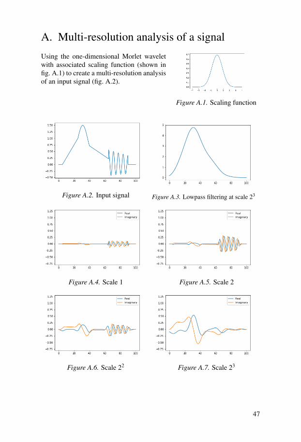
A. Multi-resolution analysis of a signal
Figure A.1. Scaling function
Using the one-dimensional Morlet waveletwith associated scaling function (shown infig. A.1) to create a multi-resolution analysisof an input signal (fig. A.2).
Figure A.2. Input signal Figure A.3. Lowpass filtering at scale 23
Figure A.4. Scale 1 Figure A.5. Scale 2
Figure A.6. Scale 22 Figure A.7. Scale 23
47
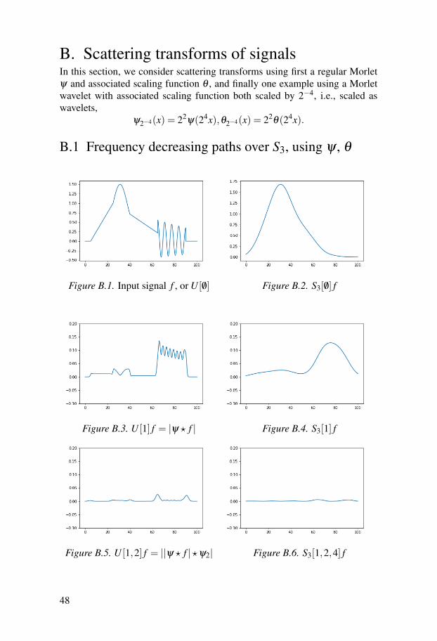
B. Scattering transforms of signalsIn this section, we consider scattering transforms using first a regular Morletψ and associated scaling function θ , and finally one example using a Morletwavelet with associated scaling function both scaled by 2−4, i.e., scaled aswavelets,
ψ2−4(x) = 22ψ(24x),θ2−4(x) = 22
θ(24x).
B.1 Frequency decreasing paths over S3, using ψ , θ
Figure B.1. Input signal f , or U [ /0] Figure B.2. S3[ /0] f
Figure B.3. U [1] f = |ψ ? f | Figure B.4. S3[1] f
Figure B.5. U [1,2] f = ||ψ ? f |?ψ2| Figure B.6. S3[1,2,4] f
48

B.2 Frequency decreasing paths over S2, using φ ,θ
Figure B.7. Input signal f , or U [ /0] Figure B.8. S2[ /0] f
Figure B.9. U [1] f = |ψ ? f | Figure B.10. S2[1] f
Figure B.11. U [1,2] f = ||ψ ? f |?ψ2| Figure B.12. S2[1,2] f
49

B.3 Constant paths over S3, using ψ,θ
Figure B.13. Input signal f , or U [ /0] Figure B.14. S3[ /0] f
Figure B.15. U [1] f = |ψ ? f | Figure B.16. S3[1] f
Figure B.17. U [1,1] f = ||ψ ? f |?ψ| Figure B.18. S3[1,1] f
50

B.4 Constant paths over S3, using ψ,θ
Figure B.19. Input signal f , or U [ /0] Figure B.20. S3[ /0] f
Figure B.21. U [2] f = |ψ2 ? f | Figure B.22. S3[2] f
Figure B.23. U [2,2] f = ||ψ2 ? f |?ψ2| Figure B.24. S3[2,2] f
51

B.5 Frequency decreasing path over S5, using ψ,θ
Figure B.25. Input signal f , or U [ /0] Figure B.26. S5[ /0] f = f ?θ25
Figure B.27. U [1] f = |ψ ? f | Figure B.28. S5[1] f
Figure B.29. U [1,2] f Figure B.30. S5[1,2] f
52

Figure B.31. U [1,2,4] f Figure B.32. S5[1,2,4] f
Figure B.33. U [1,2,4,8] f Figure B.34. S5[1,2,4,8] f
Figure B.35. U [1,2,4,8,16] f Figure B.36. S5[1,2,4,8,16] f
53

B.6 Frequency decreasing path over S5, using ψ2−4,θ2−4
Figure B.37. Input signal f , or U [ /0] Figure B.38. S5[ /0] f
Figure B.39. U [1] f Figure B.40. S5[1] f
Figure B.41. U [1,2] f Figure B.42. S5[1,2] f
54

4. References
[1] Malcolm Ritchie Adams and Victor Guillemin. Measure theory and probability.Springer, 1996.
[2] Joakim Andén and Stéphane Mallat. Deep scattering spectrum. IEEETransactions on Signal Processing, 62(16):4114–4128, 2014.
[3] Fabio Anselmi, Joel Z Leibo, Lorenzo Rosasco, Jim Mutch, Andrea Tacchetti,and Tomaso Poggio. Unsupervised learning of invariant representations inhierarchical architectures. arXiv preprint arXiv:1311.4158, 2013.
[4] Jean-Pierre Antoine, Romain Murenzi, Pierre Vandergheynst, andSyed Twareque Ali. Two-dimensional wavelets and their relatives. CambridgeUniversity Press, 2008.
[5] Ashish Bansal and Ajay Kumar. Generalized analogs of the heisenberguncertainty inequality. Journal of Inequalities and Applications, 2015(1):168,2015.
[6] Swanhild Bernstein, Jean-Luc Bouchot, Martin Reinhardt, and Bettina Heise.Generalized analytic signals in image processing: comparison, theory andapplications. In Quaternion and Clifford Fourier Transforms and Wavelets,pages 221–246. Springer, 2013.
[7] Haim Brezis. Functional analysis, Sobolev spaces and partial differentialequations. Springer Science & Business Media, 2010.
[8] Michael M Bronstein, Joan Bruna, Yann LeCun, Arthur Szlam, and PierreVandergheynst. Geometric deep learning: going beyond euclidean data. IEEESignal Processing Magazine, 34(4):18–42, 2017.
[9] Joan Bruna. Scattering representations for recognition. PhD thesis, EcolePolytechnique X, 2013.
[10] Joan Bruna and Stéphane Mallat. Invariant scattering convolution networks.IEEE transactions on pattern analysis and machine intelligence,35(8):1872–1886, 2013.
[11] Ingrid Daubechies. Ten lectures on wavelets. SIAM, 1992.[12] Jonas Gomes and Luiz Velho. From fourier analysis to wavelets. Springer,
2015.[13] Ian Goodfellow, Yoshua Bengio, and Aaron Courville. Deep Learning. MIT
Press, 2016. http://www.deeplearningbook.org.[14] Geoffrey Grimmett and David Stirzaker. Probability and random processes.
Oxford university press, 2001.[15] Kurt Hornik, Maxwell Stinchcombe, and Halbert White. Multilayer
feedforward networks are universal approximators. Neural networks,2(5):359–366, 1989.
[16] Yann LeCun, Koray Kavukcuoglu, and Clément Farabet. Convolutionalnetworks and applications in vision. In Circuits and Systems (ISCAS),Proceedings of 2010 IEEE International Symposium on, pages 253–256. IEEE,2010.
55

[17] Elliott H Lieb and Michael Loss. Analysis, volume 14 of graduate studies inmathematics. American Mathematical Society, Providence, RI,, 4, 2001.
[18] Stephane Mallat. A wavelet tour of signal processing: the sparse way.Academic press, 2008.
[19] Stéphane Mallat. Group invariant scattering. Communications on Pure andApplied Mathematics, 65(10):1331–1398, 2012.
[20] Stéphane Mallat. Understanding deep convolutional networks. Phil. Trans. R.Soc. A, 374(2065):20150203, 2016.
[21] Yves Meyer. Wavelets and operators, volume 1. Cambridge university press,1995.
[22] Edouard Oyallon, Eugene Belilovsky, and Sergey Zagoruyko. Scaling thescattering transform: Deep hybrid networks. CoRR, abs/1703.08961, 2017.
[23] Ram Shankar Pathak. The wavelet transform, volume 4. Springer Science &Business Media, 2009.
[24] Paolo Prandoni and Martin Vetterli. Signal processing for communications.Collection le savoir suisse, 2008.
[25] Bruno Torrésani. Analyse continue par ondelettes. EDP Sciences, 1995.[26] Matthew D Zeiler and Rob Fergus. Visualizing and understanding convolutional
networks. In European conference on computer vision, pages 818–833.Springer, 2014.
56