waveletextractor:a bayesianwell–tie and wavelet ......wavelets and noise parameters optimally...
TRANSCRIPT

WaveletExtractor: A Bayesian well–tie and
wavelet extraction program ⋆
James Gunning a,∗, Michael E. Glinsky b
aCSIRO Division of Petroleum Resources, Bayview Ave, Clayton, Victoria,
Australia, 3150, ph. +61 3 95458396, fax +61 3 95458380
bBHP Billiton Petroleum, 1360 Post Oak Boulevard Suite 150, Houston, Texas
77056, USA
Abstract
We introduce a new open–source toolkit for the well–tie or wavelet–extraction prob-lem of estimating seismic wavelets from seismic data, time-to-depth information, andwell–log suites. The wavelet extraction model is formulated as a Bayesian inverseproblem, and the software will simultaneously estimate wavelet coefficients, otherparameters associated with uncertainty in the time–to–depth mapping, positioningerrors in the seismic imaging, and useful amplitude–variation–with–offset (AVO) re-lated parameters in multistack extractions. It is capable of multi–well, multi–stackextractions, and uses continuous seismic data-cube interpolation to cope with theproblem of arbitrary well paths. Velocity constraints in the form of checkshot data,interpreted markers, and sonic logs are integrated in a natural way.
The Bayesian formulation allows computation of full posterior uncertainties ofthe model parameters, and the important problem of the uncertain wavelet spanis addressed uses a multi-model posterior developed from Bayesian model selectiontheory.
The wavelet extraction tool is distributed as part of the Delivery seismic inversiontoolkit. A simple log and seismic viewing tool is included in the distribution. Thecode is written in java, and thus platform independent, but the Seismic Unix (SU)data model makes the inversion particularly suited to Unix/Linux environments. Itis a natural companion piece of software to Delivery, having the capacity to producemaximum likelihood wavelet and noise estimates, but will also be of significant util-ity to practitioners wanting to produce wavelet estimates for other inversion codesor purposes. The generation of full parameter uncertainties is a crucial function forworkers wishing to investigate questions of wavelet stability before proceeding tomore advanced inversion studies.
Key words: wavelet extraction, well tie, Bayesian, seismic, signature, inversion,open–source,
Article originally published in Computers & Geosciences 32 (2006)

Contents
1 Introduction 3
2 Problem Definition 6
2.1 Preliminaries 6
2.2 Wavelet parameterization 8
2.3 Time to depth constraints 10
2.4 Log data 11
3 Forward model, likelihood, and the Bayes posterior 11
3.1 Contributions to the likelihood 13
4 Forming the posterior 14
4.1 The uncertain span problem 15
5 Questions of statistical significance 16
6 The code 17
7 Examples 18
7.1 Simple Single Reflection 18
7.2 Standard dual–well extraction 20
7.3 AVO extraction for ‘Bitters’ well 21
8 Conclusions 24
Appendix 1: Bayesian update formulas for approximate multi-Gaussianposteriors including the noise parameters 27
Appendix 2: Data input forms 29
Appendix 3: Outputs 30
Appendix 4: Issues in positional uncertainty modeling 31
⋆ Updated manuscript with additional Appendices from citation (Gunning and Glin-sky, 2006). Please cite as both (Gunning and Glinsky, 2006) and the website.∗ Corresponding author.Email address: [email protected] (James Gunning).
2
Appendix 5: Detail on the time and depth fields in the log, survey andcheckshot data, plus output time scales 33
Appendix 6: Correlated noise estimates 35
Appendix 7: Measures of noise, signal–to–noise, cross–correlation, PEP 36
Appendix 8: Alternative reflectivity expressions, stack angles, andraytracing 37
Appendix 9: Some functionality for broadband data 40
Appendix 10: Some functionality for time–lapse well ties 42
1 Introduction
The common procedure of modeling post–stack, post-migrated seismic data asa simple convolution of subsurface ‘reflectivity’ with a band–limited wavelet,and the use of this model as the basis of various probabilistic inversion algo-rithms, has been the subject of some very vigorous – and occasionally heated– debates in the last 20 years or so. It is not our intention to rehearse themany and diverse arguments at length in this article: trenchant views both insupport and opposition to this model have been expressed at length in the lit-erature (see, e.g. the series of vigorous exchanges following Ziolkowski (1991)).Many detractors believe that this approach places excessive importance onstatistical machinery at the expense of physical principles; a perfectly reason-able objection in cases where important experimental or modeling issues areoversimplified and the statistical analysis is disproportionately ornate. Whilethese criticisms can have considerable weight, our view is that inverse modelingin geophysics must always deal with uncertainty and noise, and the commu-nity seems to have come to the practical conclusion that good modeling candispense with neither solid physics nor sensible statistics.
There is a perfectly adequate theoretical justification for the convolutionalmodel, as long as absorption and reflections are sufficiently weak, and theseismic processing preserves amplitudes. Closely related assumptions must alsohold for the imaging/migration process to be meaningful; these are usuallybased on ray–tracing and the Born approximation. The migrated images willthen be pictures of the true in–situ subsurface reflectivity – albeit bandlimitedby an implied filter which embodies the wavelet we seek to extract. Sincemodern inversion/migration methods are closely related to Bayesian updatesfor the subsurface velocity model based on common image gathers (Tarantola,1984; Gouveia and Scales, 1998; Jin et al., 1992; Lambare et al., 1992, 2003), itwould be desirable if well log data were directly incorporated into the migration
3

formula. This is not commonly done, for reasons that may relate primarily tothe segregation of workflows, but also technical difficulties. There remains apractical need for wavelet extraction tools operating on data produced by themigration workflow.
Much of the skepticism about convolutional models has arisen from the ob-servation that wavelets extracted from well ties often seen to vary consider-ably over the scale of a survey. This in itself does not seem to us a sufficientargument to dismiss the model as unserviceable. Firstly, a host of reasons as-sociated with inadequacies in the seismic processing, may create such effects.For example, sometimes there is heavy attenuation from patchy shallow reefswhich is imperfectly compensated for. Secondly, it is rarely – if ever – demon-strated that the difference in wavelets extracted at different parts of the surveyis statistically significant. As before, an ideal solution would involve unifyingthe imaging problem with the well–tie problem for each new well, so imagedamplitudes are automatically constrained to log information. But until this iscommonplace, independent parties will be responsible for the seismic process-ing and well–tie workflows, so the well–tie work has to proceed with the ‘bestcase’ processed seismic data at hand. In this situation, errors in the imaginghave to be absorbed in modeling noise, and the practitioner should at leastattempt to discern if the wavelets extracted at different wells are statisticallydifferent.
It is the author’s experience that commercial wavelet extraction codes do notproceed from an explicit probabilistic approach to wavelet extraction, and thusare not capable of producing statistical output. Most appear to implement areasonable least-squares optimization of a model misfit function, but produceonly maximum-likelihood estimates (with no associated uncertainty measures),and often only cosmetically filtered versions of these. In addition, there are anumber of parameters associated with the time-to–depth mapping (henceforthcalled ’stretch–and squeeze’), multi–stack and incidence angle (AVO) effects,and imaging errors that ought in principle to be jointly optimized along withthe wavelet parameters to improve the well tie. To the authors knowledge,control of such parameters are not available in commercial codes. Many ofthe commercial programs quote the fine work of Walden and White (Waldenand White, 1998) in their pedigree. These algorithms are entirely spectrally–based, which make them very fast and well suited to (probably) impatientusers. However, the formulation is not explicitly probabilistic, and the spectralmethods will no longer hold once extra modeling parameters are introducedwhich will move the well log in space or time. More recently, a paper by Bulandand Omre (2003) presents a model very much in the same spirit as that weadvocate, but no code is supplied. Some notable differences in modeling priorityexist between our work and that of Buland. We consider the problem of theunknown wavelet span as very important, and devote considerable effort tomodeling this. Conversely, Buland puts some focus on correlated noise models
4
and assumes the wavelet span to be known apriori. It is our experience that thewavelet span, treated as an inferable parameter, couples strongly with the noiselevel, and is unlikely to be well known in a practical situation. We also prefera more agnostic approach to modeling the effective seismic noise, since this isa complex mixture of forward modeling errors, processing errors, and actualindependent instrumental noise. It seems unlikely that such a process wouldbe Gaussian, and still less susceptible of detailed modeling of the two–pointGaussian correlation function.
We have no objection in principle to the application of cosmetic post-extractionfiltering in order to improve the apparent symmetry or aesthetic appeal of ex-tracted wavelets, but feel that these requirements would be better embeddedin some kind of prior distribution in a Bayesian approach. Similarly, the re-lationship between the sonic log and any time–to–depth information derivedfrom independent sources (like a checkshot) seems most naturally expressedwith a Bayesian likelihood function.
In summary, we feel that the simple convolutional model is likely to linger onindefinitely as the standard model for performing probabilistic or stochasticinversion. It is then crucially important to ensure that inversions are run withwavelets and noise parameters optimally derived from well data, checkshotinformation and the same seismic information. There is then a considerableneed for quality software for performing well–ties using a full probabilisticmodel for the wavelet coefficients, span, time to depth parameters, and otherrelated parameters that may be required for inversion or other quantitativeinterpretations.
We present just such a model and its software implementation details in thispaper. Section 2 presents the Bayesian model specification, and suitable choicesfor the priors. The forward model, likelihoods and selection of algorithms isdiscussed in section 3, with the final posterior distribution described in sec-tion 4. Questions of statistical significance are addressed in section 5. Detailsabout the code and input/output data forms are discussed in section 6, butmost detail is relegated to the electronic appendices 2 and 3. A variety of ex-amples are presented in section 7, and some final conclusions are then offeredin section 8.
5

2 Problem Definition
2.1 Preliminaries
The wavelet extraction problem is primarily one of estimating a wavelet fromwell log data, imaged seismic data, and a time–to–depth relation that approxi-mately maps the well-log onto the seismic data in time. We will use the follow-ing forward model in the problem, with notation and motivations developedin the remainder of this section. The observed seismic Sobs is a convolution ofthe reflectivity r with a wavelet w plus noise en
Sobs(x+∆x, y +∆y, t+∆tR) = r(x, y, t|τ ) ∗w + en, (1)
taking into account any lateral positioning (∆x,∆y) and registration error ∆tRof the seismic data with respect to the well coordinates. The well log data ismapped onto the time axis using time–to–depth parameters τ .
A few remarks about the various terms of this equation are required. The im-aged seismic data Sobs is likely to have been processed to a particular (oftenzero) phase, which involves estimation of the actual source signature (gleanedfrom seafloor or salt-top reflections, or perhaps even explicit modeling of thephysics of the impulsive source), and a subsequent removal of this by decon-volution and bandpass filtering. The processed data is then characterized byan ’effective’ wavelet, which is usually more compact and symmetrical thanthe actual source signature. This processing clearly depends on the early-timesource signature, so subsequent dispersion and characteristics of the amplitudegain control (and possible inverse–Q filtering) may also make the ‘effective’wavelet at longer times rather different than the fixed wavelet established bythe processing. Since the wavelet appropriate for inversion work will be thatapplicable to a time window centered on the inversion target, it may be verydifferent in frequency content, phase and amplitude from that applicable toearlier times. Thus, we begin with the assumption that the user has relativelyweak prejudices about the wavelet shape, and any more definite knowledge canbe integrated into the well–tie problem at a later stage via appropriate priorterms.
Deviated wells impose the problem of not knowing precisely the rock propertiesin the region above and below a current point in the well, since the log isoblique. Given that a common procedure would be to krige the log valuesout into the near–well region, and assuming the transverse correlation rangeused in such kriging would be fairly long, a first approximation is to assumeno lateral variations in rock properties away from the well, so the effectiveproperties producing the seismic signal are those read from the log at theappropriate z(t). The wavelet extraction could, in principle, models errors in
6
the reflectivity calculation, which could then absorb errors associated whichthis long–correlation kriging assumption. Another way to think about thisapproximation is the leading term in a ‘near–vertical’ expansion. The seismicamplitudes to use will be those interpolated from the seismic cube at theappropriate (x, y, t(z)). In this approximation a change in the time–to–depthmapping will result in a new t′(z), but not a new (x, y). Extraction of theseamplitudes for each possible realization of the time–to–depth parameters mustbe computationally efficient.
Wavelet extraction for multiple wells will be treated as though the modelingparameters at each well are independent (e.g. time–to–depth parameters). Thelikelihood function will be a product of the likelihood over all wells. The waveletwill be modeled as transversely invariant.
The wavelet is parametrized by a suitable set of coefficients over an uncertainspan and will be naturally tapered. Determination of the wavelet span is intrin-sic to the extraction problem. The time to depth mapping from, e.g. checkshotdata, will be in general not exact, since measurement errors in first–break timesin this kind of data may not be negligible. We allow subtle deviations from theinitial mapping (‘stretch–and–squeeze’ effects) so as to improve the quality ofthe well–tie, and the extent of these deviations will be controlled by a suitableprior.
Other parameters that may be desirable to model are (1) time registrationerrors in the seismic: these are small time errors that may systematicallytranslate the seismic data in time, and (2) positioning errors: errors that maysystematically translate the seismic data transversely in space. The latter inparticular are useful in modeling the effects of migration errors when usingpost–migration seismic data. Since the wavelet extraction may be performedwith data from several wells, the positioning and registration errors may bemodeled as either (a) independent at each location, which assumes that themigration error is different in widely separated parts of the survey, or (b) syn-chronized between wells, which may be an appropriate assumption if the wellsare close.
The extraction is also expected to cope with multi-stack data. Here the syn-thetic seismic differs in each stack because of the different angle used in thelinearized Zoeppritz equations. Because of anisotropy effects, this angle is notperfectly known, and a compensation error for this angle is another parameterwhich is desirable to estimate in the wavelet extraction. Users may also believethat the wavelets associated with different stacks may be different, but related,for various reasons associated with the dispersion and variable traveltimes ofdifferent stacks. It is desirable to build in the capacity to permit stretch andscale relations between wavelets associated with different stacks
7

Finally, the extraction must produce useful estimates of the size of the seismicnoise, which is defined as the error signal at the well–tie for each stack.
2.2 Wavelet parameterization
2.2.1 Basic parameters
Let the wavelet w(aw) be parametrized by a set of coefficients aw, with suitableprior p(aw). Like Buland and Omre (2003), we use a widely dispersed Gaus-sian of mean zero for p(aw). The wavelet is parameterized in terms of a set ofequispaced samples i = −M . . .N (kW in total), spaced at the Nyquist rateassociated with the seismic band edge (typically about δt = 1/(4fpeak)). Thefirst and last samples must be zero, and the samples for the wavelet at the seis-mic data rate (e.g. 2,4 ms) are generated by cubic splines with zero-derivativeendpoint conditions. See Fig. 1. Note there are fewer fundamental parame-ters than seismic samples. This parameterization enforces sensible bandwidthconstraints and the necessary tapering. Cubic splines are a linear mapping,
-1.5 -1 -0.5 0.5 1
-0.4
-0.2
0.2
0.4
0.6
0.8
1
Fig. 1. Parameterization of wavelet in term of coefficients at Nyquist spacing asso-ciated with band edge (black boxes), and resulting coefficients generated at seismictime-sampling rate (circles) by cubic interpolation. Cubic splines enforce zero deriva-tives at the edges for smooth tapering.
so the coefficients at the seismic scale aS are related to the coarse underlyingcoefficients aW linearly. Given a maximum precursor and coda length, the twoindices M,N then define a (usually small) set of wavelet models with variablespans and centering.
For two–stack ties, the default is to assume the same wavelet is used in theforward model for all stacks. However, users may believe the stacks mightlegitimately differ in amplitude and frequency content (far-offset stacks usuallyhave about 10% less resolution than the near stack). We allow the additionalpossibility of ‘stretching and scaling’ the far wavelet (two additional parametersadded on to aw) from the near wavelet to model this situation. The priors
8

for the additional ‘stretch and scale’ factors are taken to be Gaussian, mostcommonly with means close to 1 and narrow standard deviations.
2.2.2 Wavelet phase constraints
Sensible bandwidth and tapering constraints are built into the wavelet param-eterization. Additionally, users often believe that the wavelet ought to exhibitsome particular phase characteristic, e.g. zero or constant phase. Since thewavelet phase φ is obtained directly from a Fourier transform of the waveletw = F (w(aw)) as φi = tan−1(ℑ(wi)/ℜ(wi), for frequencies indexed i, a suit-able phase–constraint contribution to the prior may be written
p(aw) ∼ exp(−∑
i
(φi(aw)− φ)2/2σ2phase)
where the sum is over the power band of the seismic spectrum (the centralfrequencies containing about 90% of the seismic energy). Here φ is a targetphase, either user-specified, or computed as 〈φi(aw)〉 if a constant (floating)phase constraint is desired. A problem with this formulation is that the branchcuts in the arctan function cause discontinuities in the prior. To avoid this, weuse the form
pphase(aw) ∼ exp(−∑
i
(D(wi, φ)2/2σ2
phase)
where D(wi, φ) is the shortest distance from the point wi to the (one-sided) rayat angle φ heading out from the origin of the complex w plane. This formulationhas no discontinuities in the error measure at branch cuts.
2.2.3 Wavelet timing
In many instances, users also believe that the peak of the wavelet responseshould occur at zero time, so timing errors will appear explicitly in the time–registration parameters, rather than being absorbed into a displaced wavelet.Very often, a zero–phase constraint is too strong a condition to impose onthe wavelet to achieve the relatively simple effect of aligning the peak arrival,since it imposes requirements of strong symmetry as well. This peak–arrivalrequirement can be built into the prior with the additional term
ppeak–arrival(aw) ∼ exp(−(tpeak(aw)− tpeak)2/2σ2
peak),
where tpeak and σpeak are user–specified numbers, and tpeak(aw) is the peaktime of the wavelet inferred from the cubic spline and analytical minimiza-tion/maximization. Clearly the peak time is only a piece–wise continuousfunction of the wavelet coefficients, so we advise the use of this constraintonly where an obvious major peak appears in the unconstrained extraction. Ifnot, the optimizer’s Newton schemes are likely to fail.
9

2.3 Time to depth constraints
2.3.1 Checkshots and markers
The primary constraint on time to depth is a series of checkshots, which pro-duce data pairs {z
(c)i , t
(c)i } with associated time uncertainty σ
(c)t,i , stemming
primarily from the detection uncertainty in the first arrival time. The depthsare measured (well–path) lengths, but convertible to true depths from the wellsurvey, and we will assume no error in this conversion. Such pairs can oftenbe sparse, e.g. 500ft spacings, and will not necessarily coincide with naturalformation boundaries. See also Appendix 5.
Markers are major points picked from the seismic trace and identified withevents in the logs. They form data triples {z
(m)i ,∆t
(m)i , σ
(m)∆t,i} which are depths
z(m) and relative timing errors ∆t(m)i with respect to the time–depth curve
associated with the linearly interpolated checkshot. The picking error is σ(m)∆t,i.
These can obviously be converted to triples {z(m)i , t
(m)i , σ
(m)t,i }, which are the
same fundamental type of data as the checkshot. Here
t(m)i = tinterpolated–from–checkshot(z
(m)i ) + ∆t
(m)i ,
and σ(m)t,i = σ
(m)∆t,i. This formula is used to convert marker data to checkshot–like
data, and is not intended to imply or induce any correlation between the twosources of information in the prior.
We use the vector τ = {t(c)i , t
(m)i } (combining checkshots and marker devi-
ations) as a suitable parameterization of the required freedom in the time–to–depth mapping. We assume that the errors at each marker or checkshotposition are independent and Normal, so the prior for the time–to–depth com-ponents becomes
p(τi) ∼ exp(−(t− t
(c,m)i )2
2σ2t,i
)
The complete time prior distribution p(τ ) =∏
i p(τi) is truncated to preservetime ordering by subtracting a large penalty from the log–prior for any stateτ that is non–monotonic.
2.3.2 Registration and positioning errors
A further possibility for error in the time to depth mapping is that the trueseismic is systematically shifted in time by a small offset. Such a registrationerror ∆tR is modeled with a Gaussian prior, and independently for each stack.Similarly, a simple lateral positioning error ∆rp = {∆x,∆y} is used to modelany migration/imaging error that may have mis–located the seismic data with
10

respect to the well position. This too is modeled by a Gaussian prior p(∆rp) ∼exp(−(∆x−∆xi)
2/2σ2∆x,i) exp(−(∆y −∆yi)
2/2σ2∆y,i) for well i. Each seismic
minicube (corresponding to each well) will have an independent error, but thiscan (optionally) be taken as the same for each stack at the well. Positioningerrors for closely spaced wells can be mapped onto the same parameter. Wewrite ∆rR = {∆tR,i,∆xi,∆yi} as the full model vector required for theseregistration and positioning errors. See also Appendix 5.
2.4 Log data
For computational efficiency during the extraction, the sonic and density logdata are first segmented into chunks whose thickness ought not to exceedλB ≈ 1/6fBE, where fBE is the upper band–edge frequency of the seismic.We use the aggregative methods of Hawkins and ten Krooden (1978) (alsoHawkins (2001(3)) to perform the blocking, based on the p–wave impedance.The effective properties of the blocked log are then computed using Backusaveraging (volume weighted arithmetic density average plus harmonic moduliaverages (Mavko et al., 1998)) yielding the triples Dwell = {vp, vs, ρ} for thesequence of upscaled layers. The shear velocity may be computed from approx-imate regressions if required (a near–stack wavelet extraction will be relativelyinsensitive to it anyway). This blocking procedure is justified by the fact thatthe convolutional response of very finely layered systems is exactly the same asthe convolutional response of the Backus–averaged upscaled system, providingthe Backus average is done to ‘first order’ in any deviations of the logs fromthe mean block values.
The raw log data and its upscaled values can be expected to have some intrinsicerror, which ultimately appears as an error er of the reflectivity values com-puted at the interfaces using the linearized Zoeppritz equations. The nature oferrors in well logging are complex in general. A small white noise componentalways exists, but the more serious errors are likely to be systematic or spa-tially clustered, like invasion effects or tool–contact problems. For this reason,we make no attempt to model the logging errors using a naive model, andexpect the logs to be carefully edited before use.
3 Forward model, likelihood, and the Bayes posterior
The forward model for the seismic is the usual convolutional model of equa-tion (23). We suppress notational baggage denoting a particular well and stack.The true reflectivity is that computed from the well log projected onto the seis-mic time axis r(x, y, t|τ ) (which is a function of the current parameters time
11

to depth map parameters τ ).
The reflection coefficients r are computed from the blocked log properties,using the linearized Zoeppritz form for the p–p reflection expanded to O(θ2)(top of p.63, Mavko et al. (1998)):
Rpp(B) =1
2
(
∆ρ
ρ+
∆vpvp
)
+Bθ2
∆vp2 vp
−2 vs
2(∆ρρ+ 2∆vs
vs
)
vp2
, (2)
with notation ρ = 12(ρ1 + ρ2), ∆ρ = ρ2 − ρ1, etc, for the wave entering layer
2 from layer 1 above (see also Appendix 8 for full Zoeppritz and Shuey alter-natives: PS reflectivities are also possible). Here, the factor B is introduced tomodel a situation where the angle θ for a given stack obtained from the Dixequation is uncertain. The stack has user–specified average stack velocity Vst,event–time Tst and stack range [Xst,min, Xst,max]. Assuming uniform weighting,the mean–square stack offset is
〈X2st〉 =
(X3st,max −X3
st,min)
3(Xst,max −Xst,min), (3)
from which the θ2 at a given interface is computed 1 as
θ2 =v2p,1
V 4stT
2st/〈X
2st〉
. (4)
Due to anisotropy and other effects related to background AVO rotation (Castagnaand Backus, 1993), the angle may not be perfectly known, so B is introducedas an additional parameter, typically Gaussian with means close to unity andsmall variance: p(B) ∼ exp(−(B − B)2/2σ2
B). The B parameter can be inde-pendent for each stack if multiple stacks are used.
The reflection Rpp is computed at all depths z where the blocked log has seg-ment boundaries, and the properties used in its calculation are the segmentproperties from Backus averaging etc. The reflection is then projected onto thetime axis using the current time to depth map and 4–point Lagrange interpo-lation. The latter approximates the reflection by placing 4 suitably weightedspikes on the 4 nearest seismic sampling points to the true projected reflectiontime (this is an approximation to true sinc interpolation, since sinc interpola-tion is far too expensive to use in an inversion/optimization problem).
1 An alternative “constant–angle” treatment of the interface incident angle is dis-cussed in Appendix 8.
12

3.1 Contributions to the likelihood
The optimization problem aims at obtaining a synthetic seismic close to theobserved data for all wells and stacks, whilst maintaining a credible velocitymodel and wavelet shape. The prior regulates the wavelet shape, so there arecontributions to the likelihood from the seismic noise and interval velocities.We address these in turn.
3.1.1 Seismic noise pdf parametrization
Physical seismic noise is largely a result of small waves with the same spec-tral character as the main signal (multiple reflections etc). However, the noiseprocess we model, en, is a mixture of this real noise and complex modelingerrors, much of the latter originated in the seismic processing. We take thisas a random signal with distribution PN(en|an), the meta–parameters an (e.g.noise level, covariance terms etc) having prior p(an).
Probably the simplest approach to the meta–parameters in the noise modelingis to avoid the issue of the noise correlations as much as possible by subsam-pling. 2 It is trivial to show that if a random process has, eg. a Ricker-2 powerspectrum (i.e. ∼ f 2 exp(−(f/fpeak)
2)), then 95% of the spectral energy in theprocess can be captured by sampling at times
∆Ts = 0.253/fpeak, (6)
where fpeak is the peak energy in the spectrum (and often about half of thebandwidth). Most practical seismic spectra will yield similar results. To keepthe meta–parameter noise description as simple as is reasonable, we chooseto model the prior distribution of the noise for stack j as Gaussian, with Nj
independent samples computed at this sampling–rate, mean zero, and overallvariance σ2
n,j . Since the variance is unknown, it must be given a suitable prior.Gelman et al. (1995) suggest a non–informative Jeffrey’s prior (PN(σn,j) ∼1/σn,j) for dispersion parameters of this type, so the overall noise likelihood +
2 If correlations in the noise are important, the simplest factorization would be totake
PN (en, σn) =1
σ2n
exp(−enT .Σ0
−1.en/2σ2n) (5)
where Σ0 is constructed from an assumed form of the correlation function, e.g. agood choice might be the Ricker–2 covariance
C(t, t′) = (1− 2π2f2peak(t− t′)2) exp(−π2f2
peak(t− t′)2),
with fpeak the peak frequency in the spectrum estimated from the seismic.
13

prior will look like
PN(en,σn) ∼ PN(en|σn)p(σn) ∼∏
stacks j
1
σNj+1n,j
exp(−en2/2σ2
n,j). (7)
Correlations between the noise level on closely spaced stacks may be significant,so we assume the user will perform multi–stack ties only on well-separatedstacks, so the priors for each stack are sensibly independent.
3.1.2 Interval velocities
Any particular state of the time depth parameter vector τ corresponds to aset of interval velocities Vint between checkshot points. It is desirable for theseto not differ too seriously from an upscaled version of the sonic log velocities.If Vint,log are the corresponding (Backus-upscaled) interval velocities from thelogs (which we treat as observables), we use the likelihood term
p(Vint,log|τ ) ∼ exp(−(Vint(τ )−Vint,log)2/2σ2
Vint)
where σVint is a tolerable interval velocity mismatch specified by the user.Typically acceptable velocity mismatches may be of the order of 5% or so,allowing for anisotropy effects, dispersion, modeling errors etc.
Even in the case that the interval velocity constraints are weak or disabled, alarge penalty term is introduced to force monotonicity in the checkshot points,since the Gaussian priors will allow an unphysical non-monotonic time-to depthmap.
4 Forming the posterior
For a given wavelet span, the Bayesian posterior for all the unknowns will thenbe
Π(aw, τ ,∆rR, B,σn) ∼
p(σn)p(B)p(aw)pphase(aw)ppeak–arrival(aw)∏
wells i
p(τi)p(∆ri) (prior)
×∏
wells i
p(Vint,log|τi) (likelihoods)
×∏
wells istacks j
PN(Sobs,ij(x+∆xi, y +∆yi, t+∆tR,i)− (rij(τi) ∗w(aw))|σn)
(8)
14

The maximum aposteriori (MAP) point of this model is then a suitable es-timate of the full set of model parameters, and the wavelet can be extractedfrom this vector. This point is found by minimizing the negative log posteriorusing either Gauss–Newton or standard Broyden–Fletcher–Goldfarb–Shanno(BFGS) methods (Nocedal and Wright, 1999; Koontz and Weiss, 1982). Theoptimizer by default is started at the prior–mean values, with typical scalesset to carefully chosen mixtures of the prior standard deviations or other suit-able scales. The parameter uncertainties are approximated by the covariancematrix formed from the quadratic approximation to the posterior at the MAPpoint, as per Appendix 1.
In some cases, especially those where registration or positioning terms exist inthe model, the posterior surface is multimodal. The code can then employ aglobal optimization algorithm formed by sorting local optimization solutionsstarted from dispersed starting points, at the user’s request. The starting pointsare distributed in a hypercube formed from the registration/positioning param-eters. This method is naturally more expensive to run than the default. Anillustration of this accompanies Example 7.2.
Where lateral positioning errors are suspected and modeled explicitly, the max-imum aposteriori parameters obtained in the optimization may not be espe-cially meaningful if the noise levels are high. Better ‘fits’ to the tie can beobtained through pure chance as easily as through correct diagnosis of a mis-positioning, and users have to beware of this subtle statistical possibility. Amore detailed discussion can be found in Appendix 4. We urge the use of thisfacility with caution.
4.1 The uncertain span problem
From the user–specified maximum precursor and coda times, a set of candidatewavelet models with indices M,N can be constructed which all lie within theacceptable bracket. These can be simply enumerated in a loop. The posteriorspace is then the joint space of models and continuous parameters, and eachmodel is of different dimensions. We treat the wavelet span problem as a model–selection problem where we seek the most likely wavelet model k (from amongthese k = 1 . . . Nm models) given the data D (D = {Sobs, Dwell}). These modelsare assumed to have equal prior weight. The maximum–aposteriori waveletmodel measured by the marginal likelihood of the model k
P (k|D) ∼∫
Π(aw, τ ,∆rR, B,σn)dawdτd∆rRdBdσn (9)
is an appropriate measure to determine the maximum likelihood wavelet. Forlinear models, it is well known that the overall model probability computed
15

from this relation (and the associated Bayes factors formed by quotients ofthese probabilities when comparing models) includes a strong tendency topenalize models that fit only marginally better than simpler models. A simpleapproximation to the integral is the standard Bayesian information criterion(BIC) penalty (Raftery, 1996), which adds a term 1
2np log(nd) to the negative
log–posterior, nd being the number of independent data points (which willbe the number of near–Nyquist samples of the noise Sobs − Ssynth when themismatch trace is digitized over the time–interval of interest), and np is thenumber of parameters in the wavelet. We do not use the BIC directly, butevaluate the integral (9) using the Laplace approximation (Raftery, 1996),based on the numerical posterior covariance matrix C obtained in Appendix 1.
Users are sometimes confused as to why long wavelets yield better ties thanshort ones, and how to choose the length. Use of the formal marginal modellikelihood immediately solves this problem: the better ties are invariably notstatistically significant. The Bayes factor concentrates the marginal likelihoodon the wavelet span of most statistical significance.
Readers unfamiliar with model–selection problems should be aware that thechoice of the prior standard deviations for the wavelet coefficients is no longerbenign when there are different size models to compare. If the prior standarddeviations are chosen too large, the model–selection probabilities suffer fromthe Lindley Paradox (Denison et al., 2002) and the posterior probability alwaysfalls on the shortest wavelet. To prevent this, the characteristic scale in theprior is chosen about 3 times larger than the RMS seismic amplitude dividedby a typical reflection coefficient.
The code computes a normalized list of all posterior wavelet–mode probabili-ties, so if the user requests realizations of the wavelet from the full posterior,these are sampled from the joint model and continuous–coefficient space. Veryoften, the posterior probability is concentrated strongly on a particular span.
5 Questions of statistical significance
Even with a sophisticated well–tie code such as that described in this paper,wavelet extraction is not a trivial workflow. In many cases, the main reflectionsin the data do not seem to correspond very well to major reflections in the welllogs, and well-matched synthetics can be produced only by switching on manydegrees of freedom, such as positioning, registration errors, and highly flexiblecheckshot points, with narrow time gates for the extraction. In such situations,the tie may well be totally spurious. A useful flag for such a situation is whenthe posterior probability lands almost entirely on the shortest wavelet, andalso when the quality of the tie degrades rapidly with increasing time gate
16

width.
There are ways to address the problem more rigorously. The usual statisticalapparatus required to detect such situations requires a forward model that cangenerate all the seismic data, and parameter uncertainties are then estimatedusing a Monte Carlo scheme, using an ensemble of extractions on a set of syn-thetic data sets. A closely related ‘null’ experiment is to generate syntheticplausible seismic data sets, totally uncorrelated from the well data, performan ensemble of extractions, and see where the true extraction falls on theMonte–Carlo distribution based on the synthetic ensemble. Strictly speaking,when we model registration or positioning errors, this scheme is possible onlyif we construct a full geostatistical earth model from which we can generaterealizations of the seismic minicube. This is a detailed, fussy piece of model-ing, requiring both categorical and continuous rock property modeling for anappreciable volume of space.
Instead, we make a ‘poor–man’s’ approximation to this model, generating seis-mic minicubes using a FFT method based on the power spectrum
S(ω) = w2z exp(−w2
z) exp(−(w2x + w2
y))
where wz is scaled from a Ricker–2 fit to the data’s average vertical powerspectrum, and wx,y are scaled so as to give a lateral correlation length specifiedby the user. The CDF of the final minicube is then mapped to that of the data,so the univariate statistics of the data minicubes are preserved. The latter stepis important, as processed seismic is not univariate Gaussian, and the waveletextraction is sensitive to amplitudes.
This Monte–Carlo test can be run in cases where the user is suspicious ofthe meaningfulness of the fit, and generates a CDF of the noise parametersobtained over the Monte–Carlo ensemble. This should have no appreciableoverlap with the true–extraction noise best estimates in cases of meaningfulties. An example is shown in section 7.3.
6 The code
The wavelet extraction code is written in java, and based largely on efficientpublic domain linear algebra 3 and optimization (Koontz and Weiss, 1982)libraries, along with the seismic handling libraries of its companion software
3 Hoschek, W., The CERN colt java library. http://dsd.lbl.gov/~hoschek/
colt/.
17
Delivery 4 . It comprises about 50k lines of source code. Wavelet extraction isa relatively light numerical application: simple extractions take seconds andmore complex problems may take minutes.
Users are expected to be able to provide seismic data in big–endian ‘minicubes’centered at each well (the seismic resides entirely in RAM), plus log data inASCII LAS or simple geoEAS format. Checkshots and well surveys in a simplegeoEAS are also required. Details of these formats are given in Appendix 2,but see also Appendix 5.
Outputs are a mixture of seismic SU 5 files for wavelets, synthetic–and–trueSU seismic pairs, and simple ASCII formats for the parameter estimationsand uncertainties. A small graphical visualization tool (extractionViewer) isprovided as part of the distribution which produces the typical cross-registeredlog and seismic displays shown in the examples. Details of the output files arein Appendix 3.
The code is available for download (Gunning and Glinsky, 2004),[3], under ageneric open–source agreement. Improvements to the code are welcome to besubmitted to the author. A set of simple examples is available in the distribu-tion, and are briefly illustrated here.
7 Examples
7.1 Simple Single Reflection
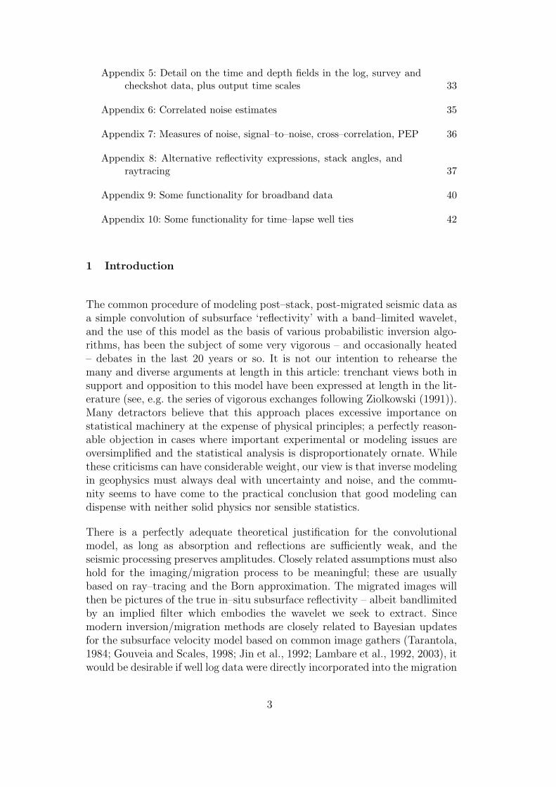
The simplest example possible is a set of logs that produce a single reflec-tion, so the synthetic trace reflects the wavelet directly. Two synthetic dataminicubes were generated from the logs with zero and a modest noise level.With the noise–free minicube, the wavelet extracts perfectly, and the poste-rior distribution converges strongly on the wavelet model just long enough tocapture the true wavelet energy.
More interesting is the extraction on the noisy minicube, shown in Fig. 2. Herethe central checkshot point was deliberately shifted 10ms, and it shares a 10msuncertainty with all the checkshot points spaced at 500ft. The naive extractedwavelet is clearly offset. A symmetrical wavelet can be forced by switching
4 Gunning, J., 2003. Delivery website: follow links from http://www.petroleum.
csiro.au.5 Cohen, J. K., Stockwell, Jr., J., 1998. CWP/SU: Seismic Unix Release 35: a freepackage for seismic research and processing,. Center for Wave Phenomena, ColoradoSchool of Mines, http://timna.mines.edu/cwpcodes.
18

on a zero–phase constraint, and the checkshot point then moves about 10msbackwards, to allow the zero–phase recovered wavelet to still generate a ‘good’synthetic.
0 0.5 1 1.5 2
rho
0 5000 10000
sonic Vp
0E0 5E3 1E4
V-interval TVD
6200
6300
6400
6500
6600
6700
6800
6900
7000
7100
7200
7300
7400
7500
7600
7700
7800
7900
8000
8100
8200
8300
8400
8500
8600
8700
8800
8900
9000
9100
9200
9300
MD
6200
6300
6400
6500
6600
6700
6800
6900
7000
7100
7200
7300
7400
7500
7600
7700
7800
7900
8000
8100
8200
8300
8400
8500
8600
8700
8800
8900
9000
9100
9200
9300
-5E-2 0E0 5E-2
synthetic
-5E-2 0E0 5E-2
seismictime(ms)
1100
1120
1140
1160
1180
1200
1220
1240
1260
1280
1300
1320
1340
1360
1380
1400
1420
1440
1460
1480
1500
1520
1540
1560
1580
1600
1620
1640
1660
1680
A) Mis-timed wavelet B) Zero-phase enforced
Fig. 2. Example of recovery of wavelet from single reflection with noisy data. A) Casewhere time-to-depth error forces mis–timing of wavelet. B) Case where phase–con-strained prior forces timing error to be absorbed in uncertain time-to-depth map.Viewing program displays co–registered time, total vertical depth (TVD), measureddepth (MD) scales for MAP (best–estimate) time-to-depth model. Also shown are (inorder) density logs ρ, sonic vp, Vint,log (interval velocity from upscaled blocked sonic),synthetic seismic (r(x, y, t|τ ) ∗w), observed seismic Sobs(x+∆x, y +∆y, t+∆tR).Viewing display can toggle on acoustic impedance, a blocked vp log, slownesses etc.
This extraction is run with the command line% waveletExtractor WaveletExtraction.xml --dump-ML-parameters
--dump-ML-synthetics --dump-ML-wavelets --fake-Vs -v 4 -c -NLR
where the main details for the extraction are specified in the XML fileWaveletExtraction.xml. The XML shows how to set up an extractionon a single trace, where the 3D interpolation is degenerate. The runtimeoptions correspond to frequently changed user preferences. Their meaningsare documented by the executable waveletExtractor in SU style self–documentation [2]. Amongst the most important options are a) those relatedto the set of wavelet spans (c.f. section 4.1): -c,-l denote respectively acentered set of wavelets, or the longest only. b) Log-data options: -NLR;assume no reflections outside log (so entire log can be used), --fake-Vs;concoct approximate fake shear log from p–wave log and density.
Standard graphical views of the MAP extraction are obtained with% extractionViewer -W MLgraphing-file.MOST LIKELY.well log.txt
and the most likely wavelet with (on a little–endian machine)% cat MLwavelet.MOST LIKELY.su | suswapbytes | suxgraph
19

7.2 Standard dual–well extraction
Here we illustrate a typical, realistic dual well extraction for two widely sep-arated wells ‘Bonnie–House’ and ‘Bonnie–Hut’. The checkshots are of highquality (bar a few points), so time—to–depth errors are confined to regis-tration effects only. We illustrate here the peak–arrival constraint prior (c.f.section 2.2.3), which forces the wavelet peak amplitude to arrive at t = 0±1ms.Multi-start global optimization was used. A Monte–Carlo study of the extrac-tion here shows the extraction to be significant with very high probability. SeeFig. 3.
0 1 2 0 2000 4000 0E0 1E3 2E3 3E3
1340
1360
1380
1400
1420
1440
1460
1480
1500
1520
1540
1560
1580
1600
1620
1640
1660
1680
1700
1720
1740
1760
1780
1800
1820
1840
1860
1880
1900
1920
1940
1960
1980
2000
2020
2040
2060
2080
2100
2120
2140
2160
1360
1380
1400
1420
1440
1460
1480
1500
1520
1540
1560
1580
1600
1620
1640
1660
1680
1700
1720
1740
1760
1780
1800
1820
1840
1860
1880
1900
1920
1940
1960
1980
2000
2020
2040
2060
2080
2100
2120
2140
2160
2180
-4E2 -2E2 0E0 2E2 4E2 -4E2 -2E2 0E0 2E2 4E2
1600
1620
1640
1660
1680
1700
1720
1740
1760
1780
1800
1820
1840
1860
1880
1900
1920
1940
1960
1980
2000
2020
2040
2060
2080
2100
2120
2140
2160
2180
2200
2220
2240
0 1 2 0 1000 2000 3000 4000 0E0 1E3 2E3 3E3
1340
1360
1380
1400
1420
1440
1460
1480
1500
1520
1540
1560
1580
1600
1620
1640
1660
1680
1700
1720
1740
1760
1780
1800
1820
1840
1860
1880
1900
1920
1940
1960
1980
2000
2020
2040
2060
2080
2100
2120
2140
2160
2180
2200
2220
2240
1360
1380
1400
1420
1440
1460
1480
1500
1520
1540
1560
1580
1600
1620
1640
1660
1680
1700
1720
1740
1760
1780
1800
1820
1840
1860
1880
1900
1920
1940
1960
1980
2000
2020
2040
2060
2080
2100
2120
2140
2160
2180
2200
2220
2240
2260
-2E2 0E0 2E2 -2E2 0E0 2E2
1600
1620
1640
1660
1680
1700
1720
1740
1760
1780
1800
1820
1840
1860
1880
1900
1920
1940
1960
1980
2000
2020
2040
2060
2080
2100
2120
2140
2160
2180
2200
2220
2240
-0.02 -0.02
0
0.02
A) B)
C) D) E)
Most likely
0
0.02
-1000 0 1000
rho sonic Vp V-interval TVD MD synthetic seismictime(ms) rho sonic Vp V-interval TVD MD synthetic seismictime(ms)
mode number0 1 2 3 4 5 6
tim
e(s
)
tim
e(s
)
Fig. 3. Example of typical dual–well extraction for ‘Bonnie’ wells: A) Tie at ‘Bon-nie–House’, B) ‘Bonnie–Hut’. Note close agreement between interval velocities andsonic logs. C) Maximum likelihood (ML) wavelet for each model–span, with MLwavelet the solid curve. D) Wavelet realizations from full posterior (section 4.1)showing small posterior uncertainty. E) Example of the acoustic impedance block-ing on a section of the Bonnie–House log.
The vertical wells ‘Bonnie–House’ and ‘Bonnie–Hut’ have relatively good qual-ity checkshots. For this reason, time–registration effects were the only unknown
20

parameters included in the time-to-depth mapping. This kind of problem cre-ates an obvious non–uniqueness in the inverse problem if the wavelet is longenough to offset itself in time by the same offset as the registration error. Theprior in the registration error in principle should remove the non-uniquenessof the global minimum in this case, but a variety of poorer local minima doappear in the problem, in which the local optimizer is easily trapped.
This problem illustrates a typical interactive workflow. 1) The extraction is per-formed with no phase or timing constraints, often for a single long wavelet (the-l option), on each well at a time. The resulting wavelets are then examinedto see if the peak response (assuming the expectation of a symmetric–lookingwavelet) is systematically shifted in time. Very bad ties may be noted, and theguilty wells excluded. 2) Large systematic offsets can then be directly enteredinto the XML file for each well (in consultation with the imaging specialist!),possibly allowing registration timing errors around the shift. 3) The individualextractions can then be rerun, confirming that major timing problems havebeen removed 4) A variety of joint–well extractions may then be attempted,perhaps turning on phase or peak–arrival constraints.
In principle, the manual setting of offsets is something that can be auto-mated as part of a (expensive) global optimization routine (available usingthe --multi-start heuristic), but users usually want to examine the well–tieson an individual basis before proceeding to joint extractions. It is often thecase that imaging around a well is suspicious for various reasons – which trans-lates into poor ties, so the best decision may be to omit the well altogether,rather than lump it into what may otherwise be a good joint extraction.
The actual extraction here is run with% waveletExtractor BonnieHousePlusBonnieHut.xml --fake-Vs
--dump-ML-parameters --dump-ML-synthetics --dump-ML-wavelets -v 4
[--constrain-peak-arrival 0 1] -c --multi-start -NLR
An illustration of the complexity of the basins of attraction is shown in Fig. 4.
7.3 AVO extraction for ‘Bitters’ well
Here we illustrate a typical single–well extraction on log data that has a strongAVO character. The two stacks are at about 5 and 30 degrees. The seismichere was generated synthetically, with a large level of white noise added tothe reflection sequence before convolution. The extraction is then of poorishquality, but still statistically significant at about the 10% level, even thoughthe most likely wavelet corresponds to the shortest model. The same waveletwas used for both stacks, so no wavelet stretch–and–scale parameters wereused.
21

-0.05
0
0.05
-0.05 0 0.05
532
534
536
538
540
542
-0.05
0
0.05
-0.05 0 0.05
t_B
onnie
House
t_BonnieHut
A) B)
Fig. 4. Example of basins of attractions for two registration parameters for Bon-nie–House and Bonnie–Hut. Grayscale represents MAP negative log–posterior valueobtained starting from the values on the axes. All other parameters are started attheir prior means. A) Basins for the problem without peak–arrival constraints B)Case with peak–arrival constraint ±1ms (--constrain-peak-arrival 0 1). Thedarkest shade is the global minimum. Note how peak–arrival term in prior greatlyenlarges basin of attraction of desired global optimum, without affecting overallMAP value.
Here the XML shows how to set up an extraction on a single seismic line,where the 3D interpolation is approximated by perpendicular ’snapping’ ontothe 2D line. The extraction module can be used to generate AVO gathers ofthe kind seen in Fig. 5a). The command% waveletExtractor Bitters.xml --dump-ML-wavelets -v 4 -NLR
--make-synthetic-AVO-gather 80 2
was used in this example, which generates 80Hz synthetics sampled at 2ms.Angles are stored in the SU header word f2. Displays can then be obtainedvia, e.g.% cat synth seis.Bitters.las.AVO-gather.su | [suswapbytes]
|suxwigb x2beg=0
The synthetic seismic minicubes are generated using the --make-synthetic
freq dt noise option, so, e.g.% waveletExtractor Bitters.xml -v 4 -NLR --dump-ML-wavelets
--make-synthetic 80 2 2.3
makes a pair of synthetic minicubes using a Ricker 2 wavelet of 80Hz bandedge, sampled at 2ms, with a noise reflectivity 2.3 times the RMS reflectionpower measured in the logs added on to the log reflectivity. The time to depthcurve is the prior mean read from the checkshot.
The second stack is specified naturally in the XML file, and the extraction
22

0 1 2
rho
0 5000
10000
15000
sonic Vp
0E
0
5E
3
1E
4
V-interval TVD
4840
4860
4880
4900
4920
4940
4960
4980
5000
5020
5040
5060
5080
51005120514051605180520052205240526052805300
5320
53405360538054005420544054605480
5500552055405560
55805600562056405660568057005720
5740
5760
5780
580058205840
5860
5880
5900
5920
5940
596059806000
6020
6040
6060
MD
5450
5500
5550
5600
5650
5700
5750
5800
5850
5900
5950
6000
6050
6100
6150
6200
6250
6300
6350
6400
6450
6500
6550
6600
6650
6700
6750
6800
6850
-2E
-1
0E
0
2E
-1
near-stacksynthetic
-2E
-1
0E
0
2E
-1
near-stackseismic
near-stackseismic
-4E
-1
-2E
-1
0E
0
2E
-1
4E
-1
far-stacksynthetic
-4E
-1
-2E
-1
0E
0
2E
-1
4E
-1
time (ms)
1420
1430
1440
1450
1460
1470
1480
1490
1500
1510
1520
1530
1540
1550
1560
1570
1580
1590
1600
1610
1620
1630
1640
1.45
1.50
1.55
1.60
1.65
0 10 20 30 40
tim
e (
s)
angle (degrees)
-0.06
-0.04
-0.02
0
0.02
0.04
0.06
0 2 4 6 8 10
-0.06
-0.04
-0.02
0
0.02
0.04
0.06
0 2 4 6 8 10
-0.02
-0.01
0
0.01
0.02
-0.5 0 0.5 1.0
A) B)
C) D) E)
mode numbermode number
tim
e(s
)
Fig. 5. A) AVO character of synthetic seismic using Ricker–2 wavelet. Note strongvariation around 1.5s. B) Two–stack extraction screen capture: far–stack syntheticand observed traces are appended at the right. C) ML wavelets vs. wavelet length(mode) with no peak–constraints. ML wavelet (boldest trace) is shortest mode. D)Same, with peak–constraints in prior. E) Recovered wavelet vs underlying waveletused to generate synthetics.
run with% waveletExtractor Bitters.xml --dump-ML-parameters
--dump-ML-synthetics --dump-ML-wavelets -v 4 -c -NLR
Significance testing is obtained by the command% waveletExtractor Bitters.xml --dump-ML-parameters
--dump-ML-synthetics --dump-ML-wavelets -v 4 -c -NLR
--monte-carlo 10
which specifies a lateral correlation length of 10 traces in the Monte–Carlo
23

synthetic minicubes. The position of the ML noise parameters with respect tothe Monte–Carlo noise parameter distribution is found by examining the fileMC ParameterSummary.txt. In this case, they sit about 10% of the way intothe Monte–Carlo distribution.
With very noisy data sets like this one, use of discontinuous or strongly non-linear terms in the likelihood such as the phase–constraint or wavelet–peakterms is somewhat dangerous. If the extraction is barely significant withoutthese constraints (a suggested first test), it will be even less so when they areadded.
8 Conclusions
We have introduced a new open–source software toolkit for performing well–ties and wavelet extraction. It can perform multi–well, deviated well, andmulti–stack ties based on imaged seismic data, standard log files, and check-shot information. Uncertainties in the time–to-depth conversion and the imag-ing and wavelet–aesthetic constraints are automatically included by the useof Bayesian techniques. The module produces maximum–apriori (’best’) es-timates of all the relevant parameters, plus measures of their uncertainty.Stochastic samples of the extracted wavelet can be produced to illustrate theuncertainty in the tie, and Monte Carlo tests of the well–tie significance canbe performed for highly suspicious ties. Our experience is that the wavelet andnoise estimates produced are of critical importance for inversion packages likeDelivery and many other applications.
Inputs for the module are common seismic data minicubes, well log files, simpleascii representations of checkshot information, and a simply–written XML fileto specify all the needed parameters. Users will be readily able to tackle theirown problems by starting from the provided examples.
The authors hope that this tool will prove useful to the geophysical and reser-voir modeling community, and encourage users to help improve the softwareor submit suggestions for improvements.
Acknowledgments
The first author gratefully acknowledges generous funding from the BHP Bil-liton technology program. Helpful comments from the two reviewers are alsoappreciated.
24

References
Aki, K., Richards, P. G., 1980. Quantitative Seismology: Theory and Methods.W. H. Freeman and Co., San Francisco.
Avseth, P., Mukerji, T., Mavko, G., 2005. Quantitative Seismic Interpretation.Cambridge University Press.
Buland, A., Omre, H., 2003. Bayesian wavelet estimation from seismic and welldata. Geophysics 68 (6), 2000–2009.
Castagna, J. P., Backus, M. M. (Eds.), 1993. Offset-dependent reflectivity –Theory and practice of AVO Analysis. Society of Exploration Geophysicists.
Denison, D. G. T., et al., 2002. Bayesian Methods for Nonlinear Classificationand Regression. Wiley.
Deutsch, C. V., Journal, A., 1998. GSLIB Geostatistical Software Library andUser’s Guide, 2nd edition. Oxford University Press.
Gelman, A., Carlin, J. B., Stern, H. S., Rubin, D. B., 1995. Bayesian DataAnalysis. Chapman and Hall.
Gouveia, W., Scales, J., 1998. Bayesian seismic waveform inversion: Param-eter estimation and uncertainty analysis. Journal of Geophysical Research103 (B2), 2759–2780.
Gunning, J., Glinsky, M., 2004. Delivery: an open-source model-based Bayesianseismic inversion program. Computers and Geosciences 30 (6), 619–636.
Gunning, J., Glinsky, M., 2006. WaveletExtractor: A Bayesian well–tie andwavelet extraction program. Computers and Geosciences 32, 681–695.
Hawkins, D. M., 2001(3). Fitting multiple change-point models to data. Com-putational Statistics and Data Analysis, 323–341.
Hawkins, D. M., ten Krooden, J. A., 1978. A review of several methods ofsegmentation. In: Gill, D., Merriam, D. (Eds.), Geomathematical and Petro-physical Studies in Sedimentology. Pergamon, pp. 117–126.
Jin, S., Madariaga, R., Virieux, J., Lambare, G., 1992. Two–DimensionalAsymptotic Iterative Elastic Inversion. Geophysical Journal International108, 575–588.
Koontz, R. S. J., Weiss, B., 1982. A modular system of algorithms for uncon-strained minimization. Tech. rep., Comp. Sci. Dept., University of Coloradoat Boulder.
Lambare, G., Operto, S., Podvin, P., Thierry, P., 2003. 3d ray+Born migra-tion/inversion – Part 1:Theory. Geophysics 68, 1348–1356.
Lambare, G., Virieux, J., Madariaga, R., Jin, S., 1992. Iterative asymptoticinversion in the acoustic approximation. Geophysics 57, 1138–1154.
Long, A. S., Reiser, C., 2014. Ultra-low frequency seismic: Benefits and solu-tions. In: Proc. International Petroleum Technology Conference,IPTC.
Mavko, G., Mukerji, T., Dvorkin, J., 1998. The Rock Physics Handbook. Cam-bridge University Press.
Nocedal, J., Wright, S. J., 1999. Numerical Optimization. Springer.Raftery, A. E., 1996. Hypothesis testing and model selection. In: Markov ChainMonte Carlo in Practice. Chapman and Hall.
25

Shuey, R. T., 1985. A simplification of the zoeppritz equations. Geophysics50 (4), 609–614.
Tarantola, A., 1984. Linearized inversion of reflection seismic data. GeophysicalProspecting 32, 998–1015.
Walden, A. T., Hosken, J. W. J., 1985. An investigation of the spectral proper-ties of primary reflection coefficients. Geophysical Prospecting 33 (3), 400–435.URL http://dx.doi.org/10.1111/j.1365-2478.1985.tb00443.x
Walden, A. T., White, R., 1998. Seismic wavelet estimation: a frequency do-main solution to a geophysical noisy input output problem. IEEE Transac-tions on Geoscience and Remote Sensing.
Zellner, A., 1986. On assessing prior distributions and Bayesian regressionanalysis with g-prior distributions. In: Bayesian Inference and Decision Tech-niques: Essays in honour of Bruno de Finetti. North–Holland, pp. 233–243.
Ziolkowski, A., 1991. Why don’t we measure seismic signatures? Geophysics56, 190–201.
26

Appendices: (supplementary material on journal archive)
Appendix 1: Bayesian update formulas for approximate multi-Gaussianposteriors including the noise parameters
The standard linear model with a Jeffreys prior on a single noise parameter hasa simple analytical posterior featuring a (right skewed) Inv–χ2 marginal distri-bution for the noise (Gelman et al., 1995, section 8.9). Although this posterioris not strictly integrable to obtain a marginal model likelihood, a Gaussianapproximation at the MAP point will be. When there are multiple noise pa-rameters and some parts of the likelihood are not scaled by the unknown noise,the posterior is somewhat messier. The amount of data commonly availablein well–tie problems is usually sufficient to make the posterior distribution ofthe noise components fairly compact, so will develop the relevant formulae onthe assumption that a full multi–Gaussian form for the joint model and noiseparameters is adequate.
Since the noise posteriors are usually right skewed, it is sensible to work interms of the joint model vector M = {m,m(n)} where m(n) is defined as
m(n)j = log(σstack j), the noise level for stack j. The non–noise components
m are formed from the wavelet components aw (and coupling parameters forthe coupled near/far wavelet mode of operation), time to depth map knots τ ,positioning and registration errors ∆rR and AVO scale term B respectively:
m ≡ {aw, τ ,∆rR, B}.
We assert a Gaussian prior for M of form P (M) = N(M, CM), where CM =diag{Cp, C
(n)p } and the C(n)
p entries for noise components m(n) are very weak(we choose the mean to be about the log of the signal RMS, and the standarddeviation large on the log scale), and absorb (for computational convenience)the Jeffrey’s noise prior and wavelet peak/phase prior terms into the collectedlikelihood
L(y|M) =PJeffreys(m
(n))
|CD(m(n))|1/2exp(−(y − f(m))TCD(m
(n))−1(y − f(m))/2).
This likelihood collects all non–Gaussian terms in (8), so y is an ‘equivalentdata’ vector, formed by the concatenation of the seismic data for all wellsand stacks, sonic–log derived interval velocities, and (from the prior) desiredphase/timing characteristics of the wavelet. Similarly f(m) is the concate-nation of the synthetic seismics, model–derived interval velocities, and thewavelet–phase/timing measures. Only that part of CD(m
(n)) pertaining to the
seismic mismatch depends on m(n). Note that CD is diagonal, with exp(2m(n)j )
terms for the seismic mismatch on stack j, σ2Vint terms for the interval veloci-
27

ties, and σ2phase, σ
2peak–arrival terms for the wavelet phase/timing.
Under the logarithmic change of variables, the Jacobian and coefficient of theabove equation conspire to yield the log-likelihood
− log(L(y|M)) = eT .m(n) +1
2(y − f(m))TCD(m
(n))−1(y − f(m)).
where ej = Nstack j, the number of seismic mismatch data points for stack j.If all terms in the log–likelihood and prior are expanded to quadratic orderin {m,m(n)} around some current guess M0 = {m0,m
(n)0 } and collected, the
resulting quadratic form corresponds to a posterior Gaussian distribution forM which may be solved using the following expressions:
∆yi =yi − fi(m0)
C1/2D,ii
(10)
Xij =fi(m0 + δmj)− fi(m0)
δmjC1/2D,ii
(sensitivity matrix from finite diffs.) (11)
Qi,j =−2δI(i),j∆yj (Nstacks× dim(y) matrix) (12)
Pij =2∑
k
(∆yk)2δI(k),iδI(k),j (Nstacks ×Nstacks matrix) (13)
where I(i) is an indicator variable that is the index of the stack–noise param-eter in m(n) that applies to component i in the ‘data’ vector y. It is zero fornon seismic–mismatch components.
With these definitions, the linear system for the model update ∆M is
C−1p + XT X −XT QT
−QX C(n)-1p + P
·
∆m
∆m(n)
=
C−1P (m−m0) + XT∆y
−e− C(n)−1p (m
(n)0 − m(n))− 1
2Q∆y
(14)
The update then has mean M′ = M0 +∆M and a covariance C which is theinverse of the coefficient matrix in (14):
C ≡
C−1p + XT X −XT QT
−QX C(n)p + P
−1
. (15)
These update formula form the basis of a Newton scheme for finding the maxi-mum aposteriori point for a particular model with wavelet vector aw. The RHSof (14) is effectively a gradient of the posterior density, so the updates vanishwhen the mode is reached. The actual implementation is a typical Gauss–Newton scheme with line searches in the Newton direction and additional
28

step-length limits applied for big Newton steps. Laplace estimates based onthe determinate of the final C are used in forming the marginal model likeli-hood.
Appendix 2: Data input forms
The data needed to perform the wavelet extraction should be in the followingforms
• Configuration file. For a particular extraction, the configuration is defined byan XML file which sets up all necessary parameter choices and file names. Itis controlled by a schema file (XSD), so configuration is simple with the BHPXML schema-driven editor supplied with the distribution. The schema islocated at au/csiro/JamesGunning/waveletextraction/xsd/ relative tothe root of the distribution, and the editor at scripts/xmledit.sh. Certainself–documenting (SU style) runtime flags are able to modify the behaviorat execution for frequently chosen options. We recommend users read theself docs carefully and follow the examples.
• Seismic data as a ‘mini–cube’, for each well, in big–endian SU format. Inline,crossline and gx,gy (group coordinate) header fields need to be correctly set.The cube should be big enough to safely enclose each well on the desiredextraction time interval, but not so large as to swamp memory (10x10 cubesare typically fine for straight holes). If x,y headers are not available, a tripletof non–collinear points can be specified in the XML file which enables thecode to map inline,crossline to x,y. Single line or trace seismic files are alsoacceptable, provided suitable flags are set in the XML.
• Log data is read in ascii, either standard ascii LAS files or the geoEASformat used by GSLIB (Deutsch and Journal, 1998). The critical depth tobe specified in these files is measured depth (MD) along the well trajectory.There must be density and DT (slowness) fields for the sonic p–wave andshear logs. A rudimentary commandline switch (--fake-Vs) will concoct aplaceholder shear log from the p–wave log if shear is not available, which isuseful for near–normal incidence extractions.
• UTM files with the well trajectories. These are geoEAS files, which musthave x, y, MD and TVD columns. Kelly bushing data will be required toconvert to true depth TVD.
• Checkshot data. Again, geoEAS format. We require MD, T, sigma T columns.• Markers (optional): geoEAS format also, with MD, T, sigma T columns.
A note on units: the code performs automatic time units detection for timedata, which is expected to be input in either s or ms. All density (mass)units cancel internally. Equation (2) involves a velocity ratio from log data tostacking–velocity Vst (see eqn (3)), and the code will again attempt to auto–
29

detect a feet vs meters difference here (logs are commonly in µS/ft, Vst maybe in m/s). Another velocity ratio occurs in (3.1.2); again, auto–detection isperformed, since Vint(τ ) is derived from a checkshot that may be imperial ormetric. The auto–detection code is based on the assumption fact that velocitieswill be specified in m/s or ft/s, and that sonic logs will be in µS/ft or (veryunusually) metric.
Users are recommended to look at the examples in the distribution closelywhen setting up their own problems.
Appendix 3: Outputs
A variety of outputs are generated by the code. Many of these are selectableby commandline switches (the code self–documents like SU codes). All SUoutputs are big–endian. In roughly diminishing order of importance, these are
• ASCII dumps of the cross-registered logs, observed and synthetic seismic, foreach well and wavelet span (typically MLgraphing-file.*). Used as directinput for the ExtractionViewer module.
• Maximum likelihood (ML) wavelet, SU format, for each wavelet span, andoverall (MLwavelet.*.su).
• ASCII files of the most likely parameter values and uncertainties (diagonalentries of the posterior covariance matrix), for each wavelet span, and overall(MLparameters.*.txt).
• Multiple realizations of the wavelets from the posterior, also SU format(wavelet realisations.su).
• Maximum likelihood 5–trace seismic sets along the well trajectory, forthe five quantities {observed–seismic, synthetic seismic, reflectivity, x, y},again, for each wavelet span, and overall (MLsynth plus true seis.*.su).These are very useful for third party software applications. Three ex-tra traces for P, S and density reflectivity (respectively) can be obtainedwith --dump-PS-reflectivity. In the notation of section 3, these termsare respectively R(p)
pp = 12(∆ρ/ρ + ∆vp/vp), R(s)
pp = 12(∆ρ/ρ + ∆vs/vs),
R(ρ)pp = 1
2(∆ρ/ρ).
If registration parameters are modelled, these files include two headerwords for delay–time:· f1 is the delay to use to plot these on the original data-minicube timescale.
· delrt is the delay to use to plot these on the shifted scale after registration-error offset.
• ASCII files for the most likely time-to–depth map, for each well, for eachwavelet span, and overall (MLtime-to-depth-map.*.txt)
• ASCII files of the most likely wavelet phase spectrum, for each wavelet span,
30

and overall (MLwavelet-phase-spectrum*).• ASCII dumps of the well log blocking (* blocked.txt).• ASCII dumps of negative log–posterior cross-sections of the posterior sur-face, shown as slices for each model parameter (posteriorXsection*.txt).These are useful for checking for possible multimodality, or serious non–linearity.
Interpretation of the time scales in these files requires some diligence; readespecially Appendix 5.
Appendix 4: Issues in positional uncertainty modeling
When using the extraction model with general positioning/registration param-eters, this amounts to using a generalized non–linear regression of form
Sobs(m) = r(m) ∗w(m) + en,
where some parameters in m determine (by continuous interpolation) the localtrace data Sobs(m) to be used in the wavelet extraction.
In this kind of model, one has to be wary of the optimization ’latching’ on to aparticularly favorable location parameter which is controlled merely by chancerather than a genuinely better fit to the regression model. A better insight intothis problem may be obtained by examining a simplified discrete ‘choose–the–data–set’ problem, in which spatial fluctuations in y are mimicked by a choiceof one of two data sets y1 or y2, and the ‘choice’ parameter is controlled by theBayes factors at the maximum likelihood point. We can then examine how theexpected fluctuations in the Bayes factor affect the uncertainty in the ‘choice’parameter by Monte–Carlo methods.
A canonical linear regression model for a specific data set y would be
y = X.m+ en
where X is the design matrix and en ∼ N(0, σ2) is the noise. The standardlikelihood is
− log(L(d|m)) ∼ (y −X.m)T (y −X.m)/2σ2 + n log(σ)
A Jeffrey’s prior for the noise variance σ2, coupled with an independent Gaus-sian N(0,Σm) for the coefficients leads to an improper posterior marginal prob-ability for the model (Gelman et al., 1995), so we use a class of conjugate priors– Zellners’ g-priors (Zellner, 1986) – which leads to simple analytic forms forthe posterior. These priors take the form
31

p(σ2)∼ 1/σ2 (16)
p(m|σ2) =N(0, gσ2(XTX)−1) (17)
where g is a single hyper-parameter. For the linear model, the posterior marginalprobability has the simple form
Π =∫
(L(d|m)p(m|σ2)p(σ2)dmdσ2 ∼ (1 + g)(n−k−1)/2(1 + g(1−R2))−(n−1)/2
where there are n data points, k parameters inm, and R2 is the usual coefficientof determination. The Bayes factor for two identical models fitted to differentdata sets (traces) y1 and y2 is then
B12 =
(
(1 + g(1−R21)
(1 + g(1−R22))
)−(n−1)/2
.
It is instructive to evaluate this quantity for realistic models of the relativefluctuation in R1 and R2 as we imagine extracting the data sets y1, y2 froma trace in a typical near–well region. To illustrate, we have fitted the ‘noisystraight line’ data sets(s)
y(1,2),i = 1 + i/n+ qi + ǫ(1,2),i i = 1, 2 . . . n
for n = 100 data points i = 1, 2 . . . n, with X describing a standard linearmodel, q ∼ N(0, 0.252) a fixed (shared) error realization of relative RMS am-plitude typical for a well–tie, and the two samples y1, y2 distinguished bythe ǫ(1,2),i term, with the setting ǫ(1,2),i ∼ N(0, 0.052) emulating small spatialfluctuations.
Different samples of y are generated by different realisations of ǫ. We haveused the recommended setting g = n to set the prior covariance g(XTX)−1
to be O(1) (see Zellner (1986) and Clyde 6 for a more extensive discussion ofthe role of g). Under this model, the Monte–Carlo distribution of B12 formedwhen y1 and y2 are drawn from different realisations of ǫ (for a fixed, randomq), is illustrated in Fig. 6. Large fluctuations in the Bayes factor associatedwith ‘position’ (of which ǫ is the surrogate) are induced by the relatively weak(5%) additional noise. It is easy to imagine that the deep local minima associ-ated with these large Bayes factors will also occur in the full nonlinear waveletextraction problem, where the ‘choice’ parameter is a continuous spatial vari-ables, rather than a discrete label. If so, it is likely that strongly constrainedpositioning parameters (associated with deep local minima in the map of theBayes factor as we move around in the near–well region) are not trustworthy.
In summary, we recommend using the lateral position modeling capabilities of
6 Clyde, M., George, E. I., 2003. Model uncertainty. Statistical and Applied Math-ematical Sciences Institute Technical Report #2003–16, see www.samsi.info.
32

-2 -1 0 1 2 3
20
40
60
80
100
log10(BF12)
frequency
Fig. 6. Variation in Bayes factor due to trace variations of the order of 5% added toa linear model. Note the logarithmic scale. The wide variations in the Bayes factorwould lead to unjustifiably strong conclusions about the optimal positioning of theseismic data if their (at least partial) origin in pure chance is not considered.
this package with extreme caution. Particular skepticism ought to be exercisedwith respect to the MAP Hessian–derived standard deviations attached to thepositioning parameters.
Appendix 5: Detail on the time and depth fields in the log, surveyand checkshot data, plus output time scales
The extraction code has two notions of depth: i) one connected to the depthcolumn of the log files (“MD”), which must be consistent between log files, thesurvey, and the checkshot, and ii) one tied to some notion of TVD (usuallysubsea (SS), for a marine survey), which is obtained from the survey files. Thelink between the two is the survey file, which contains both an MD and TVDcolumn. It doesn’t really matter where MD is measured from (e.g. the kellybushing (KB), or perhaps the surface), so long as the “MD” used in the surveyfile is the same as the “MD” in the log file and the “MD” in the checkshotfile. It also doesn’t matter exactly what the datum is for TVD; the outputsare given in TVD as well as MD for user convenience.
For time scales, the time in the checkshot must have the same meaning as thetime in the seismic minicubes, so this is usually TWT vertical (usually SS formarine data). Service companies that provide checkshot data virtually alwaysprovide a vertical TWT field and a MD field, but occasionally one is unluckyand the MD field has been lost in favour of the TVD, in which case the MDfield will need to be recovered from the TVD entries, the survey file, and someinterpolation tool such as Matlab/Mathematica. Most commonly, one ends upwith MD from KB, and TVD from SS, and TWT vertical.
33

Users need to be careful in interpreting seismic trace outputs when the stack–specific time-registration parameters are used. The parameters tagged <time -to depth local systematic time shift mean ms> in the XML file translate theseismic minicubes in time, not the checkshot data. The general parametri-sation allows for different registration errors for each stack, in which casethe registration errors cannot be simply absorbed into a single new time–to–depth mapping. But in the case that there is only one stack, or the option--synch-stacks is supplied, there is then a unique registration error applica-ble for each well, and this can in principle be absorbed into the time–to–depthmap (or checkshot). If the commandline and parameters permit such a pos-sibility, the extractor outputs will include a second time scale correspondingto the seismic minicube time scale, which will facilitate interpretations on theorigial seismic minicubes. Specifically
• The (MLsynth plus true seis.*.su) files will be written using the orig-inal seismic minicube times, with delay–time as per the f1 header word.The delrt header word passes the (shifted) delay–time scale induced by theregistration parameter (see also Appendix 3).
• The MLgraphing-file.* files have the extra seismic time scale, which theextractionViewer will display clearly.
• The MLtime-to-depth-map.*.txt files (a–posteriori time–to–depth maps)will contain an extra seismic time column.
• If requested (-b), the blocked log files (* blocked.txt) will also contain thecheckshot time scale and seismic time scale.
A further point is that extractions that use and produce non–zero time regis-tration parameters will usually require the seismic stacks to be shifted in timefor any subsequent e.g. inversion work. For independent errors at each well andstack, the registration correction are then estimated by the extraction process,and thus are “known”, but spatially variable, at only the well locations. A fullseismic volume from which the minicubes have been extracted will then haveto be resampled/re–registered using, say, a kriging map interpolating the welllocations.
In the interests of parsimony, a probably wiser choice is to use thesynchronize shifts with other well XML entry, tying all the registrationerrors for the wells to a common parameter (one per stack, or one overall if--sync-stacks is used too). The constant registration shift at all wells is thenequivalent to a shifted wavelet (if we neglect any phase or peak–arrival con-straints on the wavelet). The availability of such a wavelet then avoids havingto shift or resample the large seismic volumes that are needed for inversionwork. In situations where it is meaningful to write such an “offset” wavelet,(one well, or all wells “synchronized” as above with the first well) the codedoes so, and file names such as MLwavelet.MOST LIKELY.stack.1.offset.suare then understood to be wavelets applicable to the original seismic volumes,
34

and where the registration effects are absorbed into the wavelet.
Appendix 6: Correlated noise estimates
In the case of multi–stack extractions, the error process ∆y = y − f(m)central to the discussion of Appendix 1, which contains two blocks of entries for“near” and “far” stacks, will be correlated between stacks. (For the followingdiscussion, we use y to denote only the seismic amplitudes). This is due tocommon terms in both the forward physics model and the imaging algorithms.Since the prior information on the noise parameters is very weak, the MAPestimate of the noise σn for each stack j can be shown to be
σ2nj =
1
Nstack j
∑
i
(yi − f(m)i)2,
coinciding with the vanishing of the RHS of equation (14). Defining the matrix(∆y)ji = yji−f(m)ji for stack j and samples i running over the (subsampled)seismic–mismatch amplitudes, the full noise covariance matrix MAP estimatecan be defined as
(σ2n)jj′ =
1
Nstack
∑
i
(yji − f(m)ji)(yj′i − f(m)j′i),
taking (as is practically the case) Nstack j = Nstack for all stacks. More suc-cinctly, we can write
σ2n =
1
Nstack
∆y∆yT ,
and further define
σ2n = diag(σ2
n)1/2.ρ.diag(σ2
n)1/2,
so diag(σ2n)
1/2 is a diagonal matrix of the “noise standard deviations” andρ is a symmetric correlation–coefficient matrix (with unit diagonals) whoseoff-diagonals encapsulate the correlation between stacks. The diag(σ2
n)1/2 es-
timates appear as noise stack * entries in the MLparameters.* files, and theoff-diagonal elements of ρ are named noise corr coeff * *. Experience showsthat typical correlation–coefficient entries might be around ρ ∼ 0.3− 0.4.
Applications
Correlated noise estimates can in principle be introduced to applications likeDelivery (Gunning and Glinsky, 2004) or sparse spike inversion. In general,
35

the log–posterior or objective function will look like
χ2 =1
2∆yT .(σ2
n)−1.∆y + Bayesian prior terms or regularisation terms
and we expect the effect of increasing correlation in the stack–error-processesto decrease the precision of estimated parameters, since the extra data’s partialredundancy is being explicitly taken into account. In the limit of full correla-tion, the posterior estimates will be equivalent to only a single stack inversion.The advantage of this formalism is that it prevents the creation of artificiallyprecise estimates of inversion parameters via “double–dipping” into the data.
Appendix 7: Measures of noise, signal–to–noise, cross–correlation,PEP
It is often useful in practical work to have a set of relations for comparisonof measures of noise. The simplest definitions, for a zero–mean signal Sobs ofvariance σ2
S, and a zero–mean noise process e of variance σ2n, with modelled
data f and Sobs ≡ f +e, assuming f and e are zero–mean uncorrelated randomprocesses (E(fe) = 0, so E(S2
obs) = E(f2) + E(e2), σ2s = σ2
f + σ2n), are
• cross–correlation coefficient ρcc of Sobs, f :
ρcc =E(Sobsf)
√
E(S2obs)E(f
2)=
E((f + e)f)√
E(S2obs)(E(S
2obs)− E(e2))
=σ2S − σ2
n√
σ2s(σ
2S − σ2
n)so
ρ2cc = 1− σ2n/σ
2S = PEP
• Proportion/percent–energy–predicted (PEP)
PEP ≡ 1− σ2n/σ
2S = 1/(1 + σ2
n/σ2f ) = ρ2cc
• Signal–to–noise ratio (power)
SNRpwr ≡ σ2f/σ
2n = ρ2cc/(1− ρ2cc) = PEP/(1− PEP)
• Signal–to–noise ratio (amplitude)
SNRamp ≡ σf/σn = ρcc/√
1− ρ2cc = (PEP/(1− PEP))1/2
• Noise–to–signal ratio (power)
NSRpwr ≡ σ2n/σ
2f = 1/ρ2cc − 1 = 1/PEP− 1
• Noise–to–signal ratio (amplitude)
NSRamp ≡ σn/σf = (1/ρ2cc − 1)1/2 = (1/PEP− 1)1/2
36

Appendix 8: Alternative reflectivity expressions, stack angles, andraytracing
Reflectivities
The geophysical community has historical affections for varieties of the reflec-tivity equation (2) which are not used by default in the code. Two alternativesare provided:
• Full isotropic Zoeppritz p-p reflectivity calculations (use --Zoeppritz). Here,no small-contrast approximations are invoked: the full equation in Aki andRichards (1980) (also in Mavko et al. (1998)) for Rpp is used, and no addi-tional “B” scaling term appears in the equations.
• The isotropic Shuey approximation (Mavko et al., 1998),Shuey (1985) (use--Shuey)
Rpp =1
2
(
∆ρ
ρ+
∆vpvp
)
(18)
+B
((∆vpvp
−(2vs)
2
v2p
(
∆ρ
ρ+
2∆vsvs
)
︸ ︷︷ ︸
∆G/G
sin2(θ1)
2+
1
2
∆vpvp
sin2(θ1) tan2(θ1)
In this case, and consistent with the small-contrast approximation, we lin-earise the ∆G/G term as shown above. B should be fixed to 1 for sensibleinterpretation. The last term is O(θ41), and will only be significant for largerangles (say θ1 > 35◦).
In both cases, for larger angles, other issues related to anisotropy and effectsfrom normal-moveout can be expected to be significant here, so users are fore-warned (see e.g. the pertinent discussion in Avseth et al. (2005)).
8.0.1 PS reflectivities
When a stack is furnished 7 with the optional attribute is-PS-data=“true” theforward model will switch over to a P–S mode–conversion model. Again theassumption is that the nominated seismic minicubes represent band–limitedtrue–amplitude images of the PS reflection coefficient.
The linearised approximations for the PS reflections are again first order inproperty contrasts, but also containing the first two terms in θ (O(θ), O(θ3)).
7 E.g. an xml entry <seismic stack info is-PS-data="true">
37
They flow from the standard Aki and Richards approximations (Mavko et al.,1998). Here, the distinction between θ1 and θ = 1
2(θ1 + θ2) ignored. For sim-
plicity, the B factor is omitted here (it is rarely used, even in the PP case).With β = vs/vp, the linearisation is
Rps =−θ12
(
∆ρ
ρ+ 2β(
∆ρ
ρ+ 2
∆vsvs
)
)
+θ3112
[
(1 + 8β + 9β2)∆ρ
ρ+ β(16 + 24β)
∆vsvs
]
. (19)
When the --Zoeppritz mode is switched on, the Rps coefficient is the stan-dard plane–wave isotropic PS reflectivity as per section 3.4 (Mavko et al.,1998). There is no PS expression in Shuey (1985), but doubtless others haveinterpolated a comparable expression to his PP formula. Since the Rps Aki–Richards approximations are usually a little worse that the Rpp, I’d suggestusers wanting a better approximation than the linear+cubic formula aboveuse full Zoeppritz. At present full Zoeppritz is used for Rps if --Shuey is re-quested. At present, PS data are presumed to be imaged in PS time if theinterval–velocity constraint is used, since this uses a likelihood construct froma PP two–way time.
Angles
The default treatment of stacks corresponds to a “constant ray–parameter”behaviour, where the stack parameters associated with equation (3) definethe incident angles via ray-tracing (which appears in linearized form in equa-tion (4)).
An alternative “constant angle–stack” behaviour can be invoked by populatingthe XML attribute is-constant-angle-stack-with-angle-degrees for anyparticular stack, e.g.<seismic stack info is-constant-angle-stack-with-angle-degrees="20">.In this mode, the incident angle to every segmented–log interface is the angledeclared above, i.e. no ray–tracing is performed. If this mode is used in com-bination with full Zoeppritz, critical reflections can still occur: the reflectivityis set to zero (with strident warnings) if this happens.
In ray-tracing (default) mode in combination with either Shuey or Zoeppritz,
38

the incident angle θ1 to an interface, as computed from strict Dix 8 ,
sin(θ1) =vp,1
V 2stTst/
√
〈X2st〉
(21)
must yield a sub–critical angle, i.e. sin(θ1) < 1, so users must take care thatthe auto–segmented well logs do not contain segments of exceptionally fastvelocities which cause total internal reflection (not uncommon with e.g. thincalcited layers). Note that the default linearised reflectivity approximation usesalso linearised Dix (equation (4)), i.e. taking sin(θ) → θ, so the sub-criticalangle requirement is neither checked nor necessary. A check of the propagatingincident angle can be dumped to files named StackAngles.* using the flag--dump-angles. The angles in StackAngles.* are from strict Snell’s law, ineither linearised, Zoeppritz or Shuey mode, to help with diagnosis. The flag--eliminate-log-spikes is a rudimentary tool for removing thin high veloc-ity layers from the segmented well logs, which can be useful.
Critical reflections are much more likely in ray–tracing mode, as the tracingis more vulnerable to logging artifacts and small scale heterogeneities. Extrakinds of (unusual) critical reflections can also occur in Zoeppritz. Any flavour ofcriticality in Shuey or Zoeppritz results in copious warnings, but the offendinginterface has its reflection coefficient set to 0.
For user feedback, in default ray–tracing mode, the code writes to stdout anestimate of a typical angle (stack angle (approx., degrees) = ....), prior to thelog–segmentation, using the replacement vp,1 → Vst in (21), i.e.
sin(θapprox) =1
VstTst/√
〈X2st〉
. (22)
This might differ appreciably from the actual ray-traced angle if the firstblocked segment has a velocity average markedly different from Vst. Extractionwindows with an upper time in the middle of a ‘quiet’ shale should not sufferany significant error.
8 An alternative statement of strict Dix (21) is
sin(θ1)
vp,1=
sin(θ2)
vp,2= . . . =
√
〈X2st〉
V 2stTst
(20)
which is just Snell’s law describing raytracing through the blocked segments. In usuallinearised mode the raytracing effectively takes sin(θi)/vp,i → θi/vp,i.
39

Appendix 9: Some functionality for broadband data
Introduction
In recent years, broadband data has become popular (Long and Reiser, 2014).These surveys deploy variable–depth airgun arrays and streamer tows to helpeliminate ghost effects from the sea-surface reflections, and a broader spectrumof energy is then available for migration/inversion. There is a sizeable literaturealready, with much of it concentrating on the ghost removal issues, and low–frequency enhancements: the paper above is a good place to start.
Broadband surveys are aimed at redressing the 2-10Hz imaging gap which fallsbetween kinematic inversions (NMO/tomography) for velocity, and reflectivity–based methods, in standard streamer surveys. This conventional imaging gapraises challenges in downstream inversion workflows, which seismic survey com-panies have been understandably anxious to address. Many broadband vendorsnow supply migrated images with apparent power (in the shallow section) rightdown to a few Hz, and very often appear to flatten the reflectivity spectrum tonear–white, irrespective of any natural spectral colour the earth response mayexhibit. Typically, earth reflectivities are quite “blue”, meaning the naturalreflectivity power from well–logs falls off nearly linear with frequency (Waldenand Hosken, 1985). Increased low–frequency power appears from Q effects(dispersion), but the general hope at the well–tie end is that all non–earth–reflectivity effects (ghosts, spherical divergence, Q, airgun signature, etc) havealready been removed.
The published literature indicates that it is truly difficult to inject significantlymore energy below 7Hz, and the successes so far seem to have more to do withenhancing the S/N ratio at the low end via better ghost treatment. Since itis not uncommon to have S/N ratios of only 2 or so in the power band of thesource (say, 40Hz), and given the natural blueing tendency of log–reflectivities,it is likely that the S/N ratio under 10Hz is worse than unity, which makesextraction of statistically significant wavelet models problematic.
It has been suggested that the autocorrelation wavelet of the imaged seismicdata might be a suitable Bayesian prior for the wavelet form. I have reservationsabout this. The long–standing issues with the imaging gap in seismic inversionhas made many vendors anxious to make bold claims about the gap–fillingvirtues of broadband data. Some images seem to show such strong power inthe low–frequency end that one is tempted to wonder whether certain kindsof noise have merely been boosted to fill this gap. From an inversion angle,it is hard to see the point of imaged seismic reflectivity having spectra verydifferent from that of the earth itself. And if the spectra were rather different,
40

the use of autocorrelation wavelets as initial estimates of a suitable wavelet forinversion would be very questionable indeed.
Two functionality enhancements have been added to help wavelet estimationin broadband contexts.
• At the very low end, the log and reflectivity data are probably powerlessto inform the wavelet spectrum. Its character emerges from the low–endtaper of the instrumental response and subsequent signature–removal/zero–phasing/Wiener–shaping and Q–treatment that has occurred in the pro-cessing. This low–end decay will almost certainly suppress DC, and yield anlow–order polynomial decay for the wavelet spectrum of form W (f) ∼ f p+1,with p = 0 or p = 1 most likely. From a simple power expansion of theFourier transform representation of W (t), this polynomial decay amounts tothe wavelet–coefficient constraints
M∑
k=−N
aw,kkl = 0, l = 0 . . . p
These confine the set of wavelets to a subspace of reduced dimensional-ity. For simplicity in implementation, these are imposed by remapping theBayesian prior–precision for the wavelet coefficients in Cp = diag{σw
2} toC−1
p → C−1p + λ2XT
p .Xp/σ2w where Xp is a matrix with rows representing
the constraint equations (Xp,lk = kl, l = 0, 1 . . . p, k = −N . . .M), andλ2 = 100 an arbitrary constant which enforces the constraint tightly (butnot perfectly). This is invoked with the option -z p, e.g. -z 0.
• Published broadband signatures that have successful recovery have the char-acter of appearing almost like a perfect spike, but with long, weak, andvery smooth precursors/codas, perhaps like Fig.7. The long tails are low–
-0.2 -0.1 0 0.1 0.2t(s)
0
1
am
plit
ude
Fig. 7. Broadband wavelet
frequency character, and given the diminishing natural well–log reflectivitypower at low frequencies, they will contribute only rather modestly to syn-thetic amplitudes and any misfit improvement. Since they require numerouswavelet coefficients, the standard Bayesian evidence model–selection ma-chinery will strongly demote them unless the new coefficients yield very sig-
41

nificant misfit improvements, which is unlikely. Normally, fixed extractionswith long flexible tails tend to fill up with noise–related overfitting features.So even if these weak tails are truly present underneath the spurious fea-tures, the anti–overfitting Occamist machinery tends to overwhelm them.Roughly speaking, they demand too many degrees of freedom for marginalimprovements in data fit, at least in sample–based representation.There are some reasonable arguments to suggest that the long tails may
result from some physical processes which are inherently slow, but describ-able with very few parameters, such as the tail–decay of a low order But-terworth filter impulse response, or perhaps residual artifacts of the slowair–bubble process. So a representation of these tails in a more parsimo-nious form may help them survive the model-selection tests that usuallyfavour shorter wavelets.To this end, I have implemented a mode of inference wherein the wavelet
coefficients aw outside the interval [−T, T ] are strongly correlated and ta-pered. When this mode operates, the tail coefficients have their prior co-variance set to the simple–kriging covariance generated by the correlationstructure Cp,i,j ∼ σ2
w exp(−|i−j|/λT ), with zero values at the wavelet edges.The kriging blocks in the coda [T, Tmax] do not correlate with the precursor[Tmin,−T ], and the central values are uncorrelated. This is invoked by theoption -t T[,λT], with T in ms, and λT = 100 a default. The upshot ofthis contrivance is that the long tails are generated by many fewer effectivedegrees of freedom in the prior, and the model–selection machinery thenbegins to promote these longer models. Since the inverse of the exponentialcorrelation matrix is a sparse Laplacian–like precision matrix, this corre-lation structure is doubtless similar to that induced by the ARMA–typemodels associated with simple Butterworth filters.A suggested workflow for this feature would be to model shorter wavelets
with the feature disabled, see whether the results seem to favour a zero–phase form with possible long and weak tails, then engage the -t option.The technique amounts to a very strong and coercive model choice, so itshould be applied with caution.
Appendix 10: Some functionality for time–lapse well ties
Introduction
In time–lapse applications, an argument commonly rehearsed is that varioussystematic errors in seismic processing will cancel out in subtracting monitorand baseline seismic reflectivity images, and the difference volume will reflectchanges that have occurred in the subsurface. In cases where there are geome-chanical effects, or very thick reservoirs, this procedure is in general not valid,
42

but there are many cases where the coupling of fluid flow to stress is moder-ately weak, reservoirs are modestly thin, and the kinematics of the monitorimages can be expected to be nearly invariant. In this case, the difference im-age will mainly reflect the effects of saturation change, and it can be helpful toprovide estimates of the effective wavelet signature that explains these seismicamplitude changes.
A significant challenge is that monitor–level log data are rarely available, soan estimate of the difference wavelet usually entails augmenting the modelwith some parameters that jointly predict the state of the elastic data nearthe well at a monitor vintage. Often the near–well data can be very roughlydescribed by a “sweep zone” moving fluid contact, with saturation changesonly in the vertical region between base and monitor contact, with a profilethat depends a deal on capillarity and dynamic rates. Fairly open systemsmay have quite abrupt capillary fringes, but sometimes quite extensive fringesoccur in lower porosity systems. The simplest, naive model, is to assume an re-gion in which Gassmann’s fluid substitution may be applied, with an unknowneffective–saturation applied over the entire interval. This model is probablyfairly adequate for thinner production zones, and adds only one extra satura-tion parameter to the model, per well.
The model is simplest to understand and apply if the time–depth uncertaintyand spatial position parameters are disabled, so positioning is fixed. Underthese assumptions, the forward model amounts to
∆TLSobs(x, y, t) = ∆TLr(x, y, t|τ ) ∗w + en, (23)
where ∆TL is the monitor–base difference operation. For the reflectivity modelon the RHS, the reflectivities at base and monitor are taken to be exactly asper equation (2), except the properties at monitor–vintage are estimated byGassmann modelling in saturation. The ingredients of the model are then asfollows:
• The seismic volumes supplied by the user are difference volumes.• Users supply estimates of fluid contact times τfc,T for the base and moni-tor vintages T = 1, 2, and an initial saturation estimate. These times aremapped to depths Zfc,T from the input “mean–prior” checkshot.
• After the log in well k is automatically segmented, all segments that inter-sect the interval [Zfc,2, Zfc,1] acquire saturation–dependent elastic properties{vp, vs, ρ}(Sk). The fraction of segment j that overlaps the sweep intervalis defined to be wj ∈ [0, 1]. Each segment’s elastic properties are computedusing a saturation parameter Sk and a Gassmann/Backus difference calcula-tion from the monitor–vintage saturation, with user–supplied grain moduli,brine properties, and in–situ net–to–gross (NG) adjustment from a suppliedVSH log (which is taken as the fraction of shale in an implied horizon-tally laminated model). This model roughly captures the main nonlinearities
43

of the Gassmann and laminated–Backus effective media models. The algo-rithm below is approximate, and assumes log data has been fluid–correctedto brine–saturated conditions. It will produce nonlinear Gassmann/Backusbehaviour (with saturation) that meets the necessary conditions at the end-points, but also captures the characteristically strong nonlinearity at smallsaturations when soft fluids are used.Explicitly, new effective segment properties {v′′p,j, v
′′
s,j , ρ′′
j} are computedat saturation Sk using the following sequence. (i) Assuming the log–segmentproperties {vp,j, vs,j , ρj} are the result of a Backus average, this is invertedto yield sand–component velocities and density, using the NG estimateand a stock shale with properties vp,shale, vs,shale, ρshale. Only segments withNG> 0.1 (a plausible safe threshold) are used. (ii) The supplied stock brineand grain densities ρb, ρg are then used to estimate porosity φsand. (iii)Gassmann fluid substitution is performed using stock hydrocarbon proper-ties vp,h, ρh, brine velocity vp,b, and grain modulus Kg, to generate the newsand properties, and the Backus average is then recomputed to yield thenew effective segment properties. The same calculation is performed withbase saturation Sk,T=1 to yield {v′p,j, v
′
s,j , ρ′
j}. The final adjusted parametersused in the monitor–vintage reflectivity are then the original ones shiftedby the segment-weighted difference, e.g. vp,j → vp,j + wj(v
′′
p,j − v′p,j). Thefree variables {Sk} are added to the list of optimisation parameters. Inter-nally, they are transformed via the logit transformation S ′
k = logit(Sk) ≡log(Sk/(1 − Sk)) ∈ (−∞,∞), which then implicitly enforces the bound–constraint {0 < Sk < 1}.
• The segmented–log properties are thus functions of the saturation variable,and the well tie model is augmented to include the effect of these new satura-tion variables. The logitised variables to track saturation enforce the bounds0 < S < 1 in the resulting nonlinear optimisation.
Usage
To use this mode of the code, the xml is augmented with
• A global code chunk tagged as time lapse info which which requires spec-ification of the items· Surface files base contacts filename,monitor contacts filename of 3–columnascii data (utm x utm y TWT(ms)) for the base and monitor surfaces de-limiting the zone where saturation changes.
· Estimates of representative sand, shale, hydrocarbon, brine and grain prop-erties vp,sand, vs,sand, φsand, vp,shale, vs,shale, ρshale, vp,h, ρh, vp,b, ρb, ρg, Kg, re-spectively, for the wellbore region undergoing production. The optionalspecified gamma log can be supplied as a VSH log (entries in [0, 1]). Ifno VSH log is supplied the net–to-gross is assumed to be 1 (i.e. no shale
44

properties specified here matter: the rock is taken to be pure sand, andthe Backus average does nothing).
• There needs to be also a well–specific xml chunk time lapse well info
specifying saturation priors for each well, expressly:· Base–level saturation Sk,T=1, and prior mean Sk and standard deviationσS,k for the monitor–level saturation Sk,T=2 ∼ N(Sk, σ
2S,k) distribution.
45