NONLINEAR “WAVELET TRANSFORMS” BASED ONMEDIAN-INTERPOLATION

DAVID L. DONOHO ∗, THOMAS P.Y. YU †

Abstract. We introduce a nonlinear refinement subdivision scheme based on median-interpolation. The schemeconstructs a polynomial interpolating adjacent block medians of an underlying object. The interpolating polynomial isthen used to impute block medians at the next finer triadic scale. Perhaps surprisingly, expressions for the refinementoperator can be obtained in closed-form for the scheme interpolating by polynomials of degree D = 2. Despite thenonlinearity of this scheme, convergence and regularity can be established using techniques reminiscent of those developedin analysis of linear refinement schemes.

The refinement scheme can be deployed in multiresolution fashion to construct a nonlinear pyramid and an associatedforward and inverse transform. In this paper we discuss the basic properties of these transforms and their possible usein removing badly non-Gaussian noise. Analytic and computational results are presented to show that in the presenceof highly non-Gaussian noise, the coefficients of the nonlinear transform have much better properties than traditionalwavelet coefficients.

1. Introduction. Recent theoretical studies [14, 13] have found that the orthogonal wavelettransform offers a promising approach to noise removal. They assume that one has noisy samples ofan underlying function f

yi = f(ti) + σzi , i = 1, . . . , n,(1.1)

where (zi)ni=1 is a Gaussian white noise. In this setting, they show that one removes noise successfullyby applying a wavelet transform, thresholding the wavelet coefficients, and inverting the transform.Here ‘success’ means near-asymptotic minimaxity over a broad range of classes of smooth f . Otherefforts [18, 16] have shown that the Gaussian noise assumption can be relaxed slightly; in the presence ofnon-Gaussian noise which has sufficiently many finite moments, one can use level-dependent thresholdswhich are somewhat higher than in the Gaussian case, and continue to obtain near-minimax results,only over a somewhat reduced range of smoothness classes.

1.1. Strongly Non-Gaussian Noise. In certain settings, data exhibit strongly non-Gaussiannoise distributions; examples include analog telephony [28], radar signal processing [1], and laser radarimaging [17]. By strongly non-Gaussian we mean subject to occasional very large deviations – muchlarger than what would follow from Gaussian assumptions.

Thresholding of linear wavelet transforms does not work well with strongly non-Gaussian noise.Consider model (1.1) in a specific case: let (zi) be i.i.d. Cauchy distributed. The Cauchy distributionhas no moments

∫x`f(x)dx for ` = 1, 2, . . ., in particular neither mean nor variance.

Under this model, typical noise realizations (zi)ni=1 contain a few astonishingly large observations:the largest observation is of size O(n). (In comparison, for Gaussian noise, the largest observation isof size O(

√log(n)).) Moreover, a linear wavelet transform of i.i.d. Cauchy noise does not result in

independent, nor identically distributed wavelet coefficients. In fact, coefficients at coarser scales aremore likely to be affected by the perturbing influence of the few large noise values, and so one seesa systematically larger stochastic dispersion of coefficients at coarse scales. Invariance of distributionacross scale and O(

√log(n)) behavior of maxima are fundamental to the results on wavelet de-noising

in [13, 14]. The Cauchy situation therefore lacks key quantitative properties which were used inde-noising in the Gaussian case.

It is not just that this situation lacks properties which would make the proofs “go through”. If wetry to apply ideas which were successful under Gaussian theory we meet with abject failure, as simplecomputational examples given later will illustrate.

1.2. Median-Interpolating Pyramid Transform. Motivated by this situation, this paperdevelops a kind of nonlinear “wavelet transform”. The need to abandon linearity is clear a priori.It is well known that linearity of approach is essentially tantamount to a Gaussian assumption andthat non-Gaussian assumptions typically lead to highly nonlinear approaches. For example, maximumlikelihood estimators in classical statistical models are often linear in the Gaussian case, but highlynonlinear under Cauchy and similar assumptions.

Central to our approach is the notion of Median-Interpolating (MI) refinement scheme. Given dataabout the medians of an object on triadic blocks at a coarse scale, we predict the medians of triadic

∗DEPARTMENT OF STATISTICS, STANFORD UNIVERSITY†PROGRAM OF SCIENTIFIC COMPUTING AND COMPUTATIONAL MATHEMATICS, STANFORD

UNIVERSITY

1

blocks at the next finer scale. We do this by finding a median- interpolating polynomial – a polynomialwith the same coarse-scale block medians – and then calculating the block medians of this polynomialfor blocks at the next finer scale. The procedure is nonlinear: the interpolating polynomial is anonlinear functional of the coarse-scale meadins; and the imputed finer scale medians are nonlinearfunctionals of the interpolating polynomial. Perhaps surprisingly, in the case of interpolation byquadratic polynomials, the interpolating polynomial and its finer scale medians can both be found inclosed form.

Using MI refinement, we can build foward and inverse transforms which can be computed rapidlyand which exhibit favorable robustness and regularity properties.

The forward transform deploys the median in a multiresolution pyramid; it computes “blockmedians” over all triadic cells. MI refinement is used to predict medians of finer scale blocks fromcoarser scale blocks; the resulting prediction errors are recorded as transform coefficients.

The inverse transform undoes this process; using coarser-scale coefficients it builds MI predictionsof finer-scale coefficients; adding in the prediction errors recorded in the transform array leads to exactreconstruction.

This way of building transforms from refinement schemes is similar to the way interpolatingwavelet transforms are built from Deslauriers-Dubuc interpolating schemes in [9] and in the waybiorthogonal wavelet transforms are built from average-interpolating refinement in [10]. The basicidea is to use data at coarser scales to predict data at finer scales, and to record the prediction errorsas coefficients associated with the finer scales. Despite structural similarities our MI-based transfomsexhibit important differences:

• Both the forward and inverse transforms can be nonlinear;• The transforms are based on a triadic pyramid and a 3-to-1 decimation scheme;• The transforms are expansive (they map n data into ∼ 3/2n coefficients).

Terminologically, because the forward transform is expansive, it should be called a pyramid trans-form rather than a wavelet transform. We call the transform itself the median-interpolating pyramidtransform (MIPT).

The bulk of our paper is devoted to analysis establishing two key properties of these transforms.• Regularity. Take block medians at a single level and refine to successively finer and finer

levels using the quadratic polynomial MI scheme. Detailed analysis shows that the successiverefinements converge uniformly to a continuous limit with Holder-α regularity for some α > 0.We prove that α > .0997 and we give computational and analytical evidence pointing toα > 1− ε for ε > 0.This result shows that MIPT has important similarities to linear wavelet and pyramid trans-forms. For example, it provides a notion of nonlinear multi-resolution analysis: just as inthe linear MRA case, one can decompose an object into ‘resolution levels’ and examine thecontributions of different different levels separately; each level contributes a regular curve os-cillating with wavelength comparable to the given resolution, with large oscillations in thespatial vicinity of significant features.• Robustness. It is well known that the median is robust against heavy-tailed noise distributions

[19, 20]. In the present setting this phenomenon registers as follows. We are able to derivethresholds for noise removal in the MIPT which work well for all distributions in rather largeclasses, irrespective of the heaviness of the tails. In particular, we show that at all but the finestscales, the same thresholds work for both Gaussian and Cauchy data. Hence a noise-removalscheme based on thresholding of MIPT coefficients depends only very weakly on assumptionsabout noise distribution.

There is considerable applied interest in developing median-based multiscale transforms, as onecan see from [2, 21, 26, 27, 24]. The analysis we give here suggests that our framework will turn outto have strong theoretical justification and may provide applied workers with helpful new tools.

1.3. Contents. Section 2 introduces the notion of median-interpolating refinement, shows howone of the simplest instances may be computed efficiently, gives computational examples and provessome basic properties. Section 3 establishes convergence and smoothness results for the quadraticmedian-interpolating refinement scheme. Section 4 develops a nonlinear pyramid transform and de-scribes properties of transform coefficients. Proofs of these properties are recorded in Section 6. Section5 applies the pyramid transform to the problem of removing highly non-Gaussian noise.

2. Median-Interpolating Refinement Schemes. In this section we describe a notion of two-scale refinement which is nonlinear in general, and which yields an interesting analog of the refinementschemes occurring in the theory of biorthogonal wavelets.

2

2.1. Median-Interpolation. Given a function f on an interval I, let med(f |I) denote a medianof f for the interval I, defined by

med(f |I) = inf{µ : m(t ∈ I : f(t) ≥ µ) ≥ m(t ∈ I : f(t) ≤ µ)}.(2.1)

Now suppose we are given a triadic array {mj,k}3j−1k=0 of numbers representing the medians of f

on the triadic intervals Ij,k = [k3−j , (k + 1)3−j):

mj,k = med(f |Ij,k) 0 ≤ k ≤ 3j .

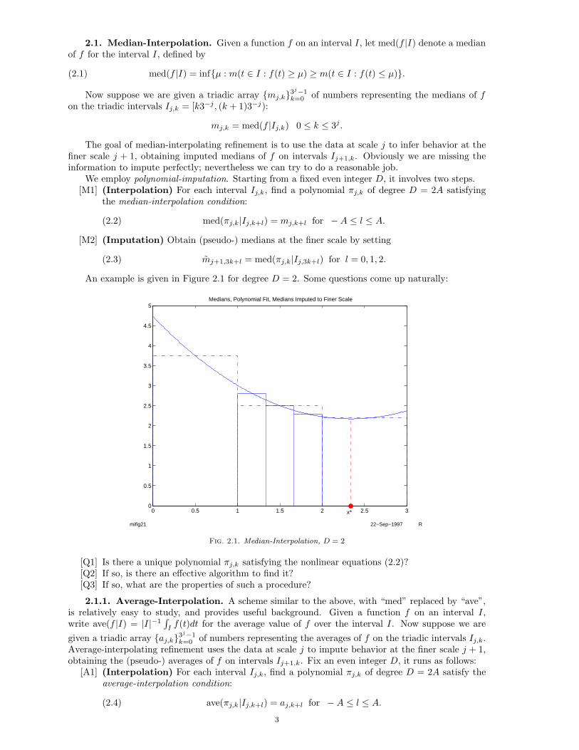
The goal of median-interpolating refinement is to use the data at scale j to infer behavior at thefiner scale j + 1, obtaining imputed medians of f on intervals Ij+1,k. Obviously we are missing theinformation to impute perfectly; nevertheless we can try to do a reasonable job.

We employ polynomial-imputation. Starting from a fixed even integer D, it involves two steps.[M1] (Interpolation) For each interval Ij,k, find a polynomial πj,k of degree D = 2A satisfying

the median-interpolation condition:

med(πj,k|Ij,k+l) = mj,k+l for −A ≤ l ≤ A.(2.2)

[M2] (Imputation) Obtain (pseudo-) medians at the finer scale by setting

mj+1,3k+l = med(πj,k|Ij,3k+l) for l = 0, 1, 2.(2.3)

An example is given in Figure 2.1 for degree D = 2. Some questions come up naturally:

0 0.5 1 1.5 2 2.5 30

0.5

1

1.5

2

2.5

3

3.5

4

4.5

5Medians, Polynomial Fit, Medians Imputed to Finer Scale

x*

mifig21 22−Sep−1997 R

Fig. 2.1. Median-Interpolation, D = 2

[Q1] Is there a unique polynomial πj,k satisfying the nonlinear equations (2.2)?[Q2] If so, is there an effective algorithm to find it?[Q3] If so, what are the properties of such a procedure?

2.1.1. Average-Interpolation. A scheme similar to the above, with “med” replaced by “ave”,is relatively easy to study, and provides useful background. Given a function f on an interval I,write ave(f |I) = |I|−1

∫If(t)dt for the average value of f over the interval I. Now suppose we are

given a triadic array {aj,k}3j−1k=0 of numbers representing the averages of f on the triadic intervals Ij,k.

Average-interpolating refinement uses the data at scale j to impute behavior at the finer scale j + 1,obtaining the (pseudo-) averages of f on intervals Ij+1,k. Fix an even integer D, it runs as follows:

[A1] (Interpolation) For each interval Ij,k, find a polynomial πj,k of degree D = 2A satisfy theaverage-interpolation condition:

ave(πj,k|Ij,k+l) = aj,k+l for −A ≤ l ≤ A.(2.4)

3

[A2] (Imputation) Obtain (pseudo-) cell averages at the finer scale by setting

aj+1,3k+l = ave(πj,k|Ij,3k+l) for l = 0, 1, 2.(2.5)

This type of procedure has been implemented and studied in (the dyadic case) [10, 11]. Theanalogs of questions [Q1]-[Q2] have straightforward “Yes” answers. For any degree D one can findcoefficients c(D)

h,l for which

aj+1,3k+l =A∑

h=−Ac(D)h,l aj,k+h, l = 0, 1, 2,(2.6)

exhibiting the fine-scale imputed averages aj+1,k’s as linear functionals of the coarse-scale averagesaj,k. Moreover, using analytic tools developed in wavelet theory [4] and in refinement subdivisionschemes [8, 15] one can establish various nice properties of refinement by average-interpolation – seebelow.

2.1.2. D = 0. We return to median-interpolation. The case D = 0 is the simplest by far; in thatcase one is fitting a constant function πj,k(t) = Const. Hence A = 0, and (2.2) becomes πj,k(t) = mj,k.The imputation step (2.3) then yields mj+1,3k+l = mj,k for l = 0, 1, 2. Hence refinement proceeds byimputing a constant behavior at finer scales.

2.1.3. D = 2. The next simplest case is D = 2, and it is the one we mainly study in this paper.To apply (2.2) with A = 1, we must find a quadratic polynomial solving

med(πj,k|Ij,k+l) = mj,k+l for l = −1, 0, 1.(2.7)

In general this is a system of nonlinear equations. One can ask [Q1]-[Q3] above for this system. Theanswers come by studying the operator Π(2) : R3 → R3 defined as the solution to the problem: given[m1,m2,m3], find [a, b, c] such that the quadratic polynomial π(x) = a+ bx+ cx2 satisfies

med(π|[0, 1]) = m1,(2.8)

med(π|[1, 2]) = m2,(2.9)

med(π|[2, 3]) = m3.(2.10)

In this section, we work out explicit algebraic formulae for Π(2). It will follow from these that (2.7)has an unique solution, for every m1,m2,m3 and that this solution is a Lipschitz functional of the mi.

Π(2) possesses two purely formal invariance properties which are of use to us.• Reversal Equivariance. If Π(2)(m1,m2,m3) = a+ bx+ cx2 then Π(2)(m3,m2,m1) = a+ b(3−x) + c(3− x)2.• Affine Equivariance. If Π(2)(m1,m2,m3) = π then Π(2)(a+ bm1, a+ bm2, a+ bm3) = a+ bπ.

Reversal equivariance is, of course, tied to the fact that median-interpolation is a spatially symmetricoperation. From affine equivariance, it follows that when m2 −m1 6= 0 we have

Π(2)(m1,m2,m3) = m1 + Π(2)(0,m2 −m1,m3 −m1)

= m1 + (m2 −m1)Π(2)(0, 1, 1 +m3 −m2

m2 −m1).(2.11)

Thus Π(2) is characterized by its action on very special triples; it is enough to study the univariatefunction Π(2)(0, 1, 1 + d) , d ∈ R. (The exceptional case when m2 −m1 = 0 can be handled easily; seethe discussion after the proof of Proposition 2.2.)

To translate equations (2.8)-(2.10) into manageable algebraic equations, we begin withProposition 2.1. (Median-Imputation, D = 2) Suppose the quadratic polynomial π(x) has

its extremum at x∗. Let s = q − p.[L] If x∗ /∈ [p+ s/4, p+ 3s/4], then

med(π(x)|[p, q]) = π((p+ q)/2)(2.12)

[N] If x∗ ∈ [p+ s/4, p+ 3s/4], then

med(π(x)|[p, q]) = π(x∗ ± s/4).(2.13)

4

Proof. We assume x∗ is a minimizer (the case of a maximizer being similar). The key fact is thatπ(x), being a quadratic polynomial, is symmetric about x∗ and monotone increasing in |x− x∗|.

If x∗ ∈ [p + s/4, p + 3s/4], then [x∗ − s/4, x∗ + s/4] ⊆ [p, q], {x ∈ [p, q] | π(x) ≤ π(x∗ ± s/4)} =[x∗−s/4, x∗+s/4]. Thus m{x ∈ [p, q] | π(x) ≤ π(x∗±s/4)} = s/2 = m{x ∈ [p, q] | π(x) ≥ π(x∗±s/4)},which implies med(π(x)|[p, q]) = π(x∗ ± s/4).

If x∗ < p + s/4 , then {x ∈ [p, q] | π(x) ≤ π((p + q)/2)} = [p, p + s/2] and {x ∈ [p, q] | π(x) ≥π((p + q)/2)} = [p + s/2, q] have equal measure. Thus med(π(x)|[p, q]) = π((p + q)/2).The sameconclusion holds when x∗ > p+ 3s/4. Thus we have (2.12). 2

The two cases identified above will be called the ‘Linear’ and ‘Nonlinear’ cases. Equations (2.8)-(2.10) always give rise to a system of three algebraic equations in three variables a, b, c. Linearityrefers to dependence on these variables. When (2.13) is invoked, x∗ = −b/2c, and so the evaluation ofπ – at a location depending on x∗ – is a nonlinear functional.

A similar division into cases occurs when we consider median interpolation.Proposition 2.2. (Median-Interpolation, D = 2) Π(2)(0, 1, 1 + d) = a + bx + cx2 can be

computed by the following formulae:[N1] If 7

3 ≤ d ≤ 5, then x∗ ∈ [ 14 ,

34 ], and

a = 11 +72d− 5

2r, b = −32

3− 13

3d+

83r, c =

83

+43d− 2

3r,(2.14)

where r =√

16 + 16d+ d2.[N2] If 1

5 ≤ d ≤37 , then x∗ ∈ [ 9

4 ,114 ], and

a = 11 +72d− 5

2r, b = −32

3− 13

3d+

83r, c =

83

+43d− 2

3r,(2.15)

where r =√

1 + 16d+ 16d2.[N3] If −3 ≤ d ≤ − 1

3 , then x∗ ∈ [ 54 ,

74 ], and

a = − 712

+112d+

r

12, b =

1310− 3

10d− r

5, c = − 4

15+

415d+

r

15,(2.16)

where r = −√

1− 62d+ d2.[L] In all other cases,

a = −78

+38d, b = 2− d, c = −1

2+d

2.(2.17)

Proof. Fix a polynomial π. To calculate its block medians on blocks [0, 1], [1, 2], [2, 3], we canapply Proposition 2.1 successively to the choices [p, q] = [0, 1], [1, 2], [2, 3]. We see that either theextremum of π lies in the middle half of one of the three intervals [0, 1], [1, 2], [2, 3] or it does not. Ifit does not lie in the middle half of any interval, the relation of the block medians to the coefficientsis linear. If it does lie in the middle half of some interval, the relation of the block medians to thecoefficients will be linear in two of the blocks – those where the extremum does not lie – and nonlinear inthe block where the extremum does lie. Hence there are four basic cases to consider: (i) x∗ ∈ [1/4, 3/4],(ii) x∗ ∈ [9/4, 11/4], (iii) x∗ ∈ [5/4, 7/4] and (iv) x∗ /∈ [1/4, 3/4] ∪ [9/4, 11/4] ∪ [5/4, 7/4]. The firstthree involve some form of nonlinearity; the remaining case is linear.

Now to solve for a polynomial π with prescribed block medians, we can see at this point thatif we knew in advance the value of x∗(π), we could identify one of Cases (i)-(iv) as being operative.It is easy to set up for any one of these cases a system of algebraic equations defining the desiredquadratic polynomial. By writing down the system explicitly and solving it, either by hand or withthe assistance of an algebraic software tool, we can obtain explicit formulae for the coefficients π. Thishas been done for Cases (i)-(iv) and results are recorded above in (2.14)-(2.17). We omit the detailedcalculation.

At this point, we have identified four different cases relating polynomials to their block medians.Within a given case, the relationship between a polynomial and its block medians is one-one. However,it remains for the moment at least conceivable that for a given collection of block medians, there wouldbe two different cases which gave the same block medians, and hence nonunique interpolation.

We are rescued by a small miracle: with six exceptions, a given set of block medians is consistentwith exactly one of the four cases.

5

To understand this, note that each of the four cases, involving a hypothesis on x∗, is consistentwith block medians [0, 1, 1 +d] only for a special set of values of d. We now proceed to identify the setof values of d which may arise in each given case, case by case (but out of numerical order). Startingwith Case (iv), we can show that if x∗ /∈ [1/4, 3/4] ∪ [9/4, 11/4] ∪ [5/4, 7/4], then the associated blockmedians [0, 1, 1 + d] must obey d /∈ [7/3, 5] ∪ [1/5, 3/7] ∪ [−3,−1/3] . As we are in Case (iv), formula(2.17) gives Π(2)(0, 1, 1 + d) = (−7/8 + 3/8d) + (2− d)x+ ((d− 1)/2)x2, and hence

x∗ = (d− 2)/(d− 1).(2.18)

By a routine calculation, Case (iv) and (2.18) combine to conclude that d /∈ [−3,−1/3] ∪ [1/5, 3/7] ∪[7/3, 5]. For future reference, set L = ([−3,−1/3] ∪ [1/5, 3/7] ∪ [7/3, 5])c.

Now turn to Case (i); we can show that if x∗ ∈ [1/4, 3/4], then the associated block medians[0, 1, 1 + d] must obey d ∈ [7/3, 5]. As we are in Case (i), formula (2.14) applies, and

x∗ =32 + 13d− 8

√16 + 16d+ d2

4(4 + 2d−√

16 + 16d+ d2).(2.19)

This and x∗ ∈ [1/4, 3/4] combine to conclude that d ∈ [7/3, 5]. For future reference, set N1 = [7/3, 5].Similar calculations show that in Case (ii) we have if x∗ ∈ [9/4, 11/4], then the associated block

medians [0, 1, 1 + d] must obey d ∈ N2 ≡ [1/5, 3/7]. Also in Case (iii) we have if x∗ ∈ [5/4, 7/4] thenthe associated block medians [0, 1, 1 + d] must obey d ∈ N3 ≡ [−3,−1/3].

We now have a collection of 4 sets: L and Ni, i = 1, 2, 3. The sets have disjoint interiors, andtogether cover the whole range of possible values for d. For d in the interior of one of these sets,exactly one of the four cases is able to generate the block medians [0, 1, 1 + d]. The exceptional valuesof d, not in the interior of one of the sets, lie in the intersection of one of the nonlinear branches Niand the linear branch L. They are −3,−1/3, 1/5, 3/7, 7/3, 5. Analysis ‘by hand’ shows that at eachexceptional value of d, the formula for Case (iv) and the formula for the appropriate Case (i)-(iii) giveidentical polynomials.

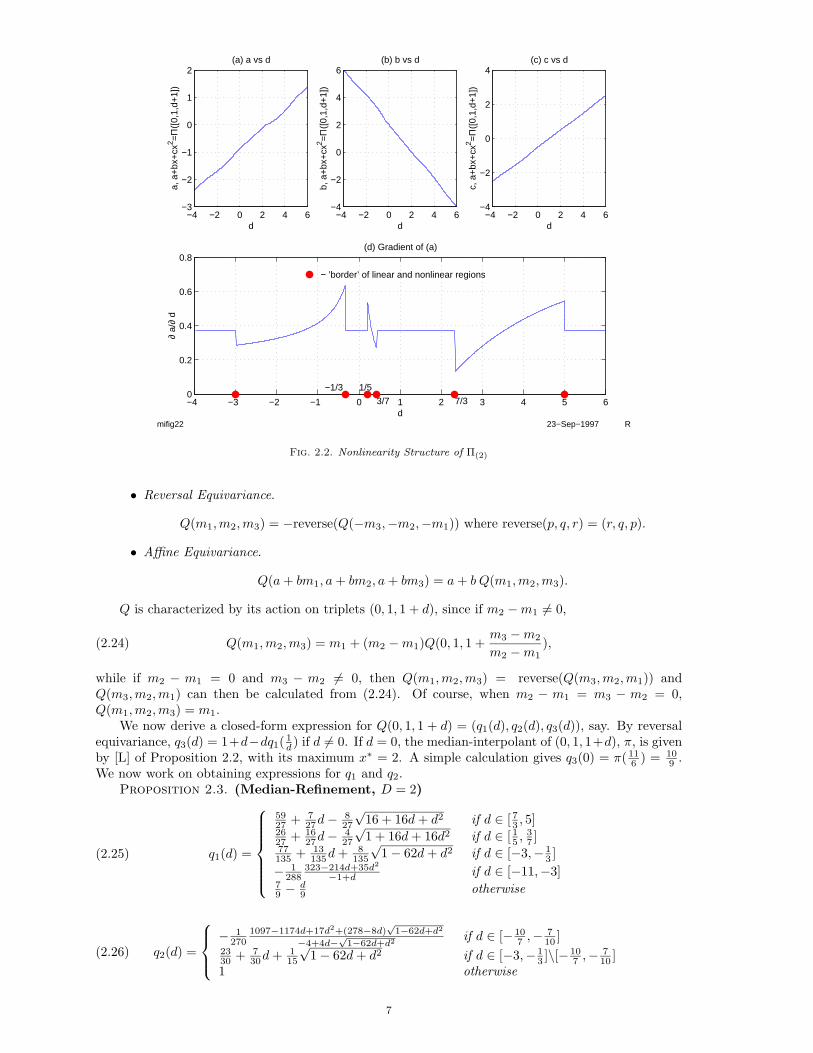
This means, among other things, that the formulas listed above cohere globally. Each individualformula gives a(d), b(d), and c(d) valid on the hypothesis that x∗ lies in a certain range; but because ofthe “small miracle”, the different formulas join continuously, producing globally monotone functionsof d. See Figure 2.2. 2

The degenerate case m2 − m1 = 0 can be handled as follows: (i) if m1 = m2 = m3, thenΠ(2)(m1,m2,m3) = m1; (ii) otherwise m3 −m2 6= 0, then use reversal equivariance followed by theformulae in Proposition 2.2. Notice that [N1]-[N3] are nonlinear rules, whereas [L] is linear. Figure 2.2illustrates the nonlinearity of Π(2). Panels (a)-(c) show a(d), b(d) and c(d), where a(d)+b(d)x+c(d)x2 =Π(2)(0, 1, d+ 1). Panel (d) shows ∂a/∂d. Proposition 2.2 implies that Π(2) is basically linear outside

N = {[m1,m2,m3] | m3 −m2

m2 −m1∈ N0},(2.20)

where

N0 = [−3,−1/3] ∪ [1/5, 3/7] ∪ [7/3, 5].(2.21)

Precisely, if µ, β, aµ+ bβ ∈ N c , then

Π(2)(aµ+ bβ) = aΠ(2)(µ) + bΠ(2)(β)

Figure 2.2(d) illustrates this point.We now combine Propositions 2.1 and 2.2 to obtain closed-form expressions for the two-scale

median-interpolating refinement operator in the quadratic case. First of all, Proposition 2.1 implies thewell-posedness of median-interpolation in the case D = 2. Hence there exists a median-interpolatingrefinement operator Q : R3 → R3 such that if π = πj,k is the fitted polynomial satisfying

med(π|Ij,k+l) = ml for − 1 ≤ l ≤ 1.(2.22)

then

Q([m−1,m0,m1]) = [med(π|Ij,3k),med(π|Ij,3k+1),med(π|Ij,3k+2)].(2.23)

Note that the refinement calculation is independent of the scale and spatial indices j and k, so Q isindeed a map from R3 to R3.

The operator Q shares two equivariance properties with Π(2):6

−4 −2 0 2 4 6−3

−2

−1

0

1

2

d

a, a

+bx

+cx

2 =Π

([0,

1,d+

1])

(a) a vs d

−4 −2 0 2 4 6−4

−2

0

2

4

6

d

b, a

+bx

+cx

2 =Π

([0,

1,d+

1])

(b) b vs d

−4 −2 0 2 4 6−4

−2

0

2

4

d

c, a

+bx

+cx

2 =Π

([0,

1,d+

1])

(c) c vs d

−4 −3 −2 −1 0 1 2 3 4 5 60

0.2

0.4

0.6

0.8

d

∂ a/

∂ d

(d) Gradient of (a)

−1/3 1/5

3/7 7/3

− ’border’ of linear and nonlinear regions

mifig22 23−Sep−1997 R

Fig. 2.2. Nonlinearity Structure of Π(2)

• Reversal Equivariance.

Q(m1,m2,m3) = −reverse(Q(−m3,−m2,−m1)) where reverse(p, q, r) = (r, q, p).

• Affine Equivariance.

Q(a+ bm1, a+ bm2, a+ bm3) = a+ b Q(m1,m2,m3).

Q is characterized by its action on triplets (0, 1, 1 + d), since if m2 −m1 6= 0,

Q(m1,m2,m3) = m1 + (m2 −m1)Q(0, 1, 1 +m3 −m2

m2 −m1),(2.24)

while if m2 − m1 = 0 and m3 − m2 6= 0, then Q(m1,m2,m3) = reverse(Q(m3,m2,m1)) andQ(m3,m2,m1) can then be calculated from (2.24). Of course, when m2 − m1 = m3 − m2 = 0,Q(m1,m2,m3) = m1.

We now derive a closed-form expression for Q(0, 1, 1 + d) = (q1(d), q2(d), q3(d)), say. By reversalequivariance, q3(d) = 1+d−dq1( 1

d ) if d 6= 0. If d = 0, the median-interpolant of (0, 1, 1+d), π, is givenby [L] of Proposition 2.2, with its maximum x∗ = 2. A simple calculation gives q3(0) = π( 11

6 ) = 109 .

We now work on obtaining expressions for q1 and q2.Proposition 2.3. (Median-Refinement, D = 2)

q1(d) =

5927 + 7

27d−827

√16 + 16d+ d2 if d ∈ [ 7

3 , 5]2627 + 16

27d−427

√1 + 16d+ 16d2 if d ∈ [ 1

5 ,37 ]

77135 + 13

135d+ 8135

√1− 62d+ d2 if d ∈ [−3,− 1

3 ]− 1

288323−214d+35d2

−1+d if d ∈ [−11,−3]79 −

d9 otherwise

(2.25)

q2(d) =

− 1

2701097−1174d+17d2+(278−8d)

√1−62d+d2

−4+4d−√

1−62d+d2 if d ∈ [− 107 ,−

710 ]

2330 + 7

30d+ 115

√1− 62d+ d2 if d ∈ [−3,− 1

3 ]\[− 107 ,−

710 ]

1 otherwise(2.26)

7

Proof. Let π denote the median-interpolant of (0, 1, 1+d) associated to intervals [0, 1], [1, 2], [2, 3].Recall that median-interpolation follows four branches [N1-3] and [L] (cf. Proposition 2.2), whereasmedian-imputation follows two branches [N] and [L] (cf. Proposition 2.1.) The main task is toidentify ranges of d for which median-interpolation and median-imputation use specific combinationsof branches. The refinement result can then be described by obtaining algebraic expressions for eachof those ranges. The calculations are similar to those in the proof of Proposition 2.2.

For q1, there are five distinct cases:1. d ∈ [ 7

3 , 5]⇒ x∗ ∈ [ 14 ,

34 ]: interpolation by branch [N1] and imputation by branch [L]

2. d ∈ [ 15 ,

37 ]⇒ x∗ ∈ [ 9

4 ,114 ]: interpolation by branch [N2] and imputation by branch [L]

3. d ∈ [−3,− 13 ]⇒ x∗ ∈ [ 5

4 ,74 ]: interpolation by branch [N3] and imputation by branch [L]

4. d ∈ [−11,−3]⇒ x∗ ∈ [ 1312 ,

54 ]: interpolation by branch [L] and imputation by branch [N]

5. d /∈ [ 73 , 5] ∪ [ 1

5 ,37 ] ∪ [−3,− 1

3 ] ∪ [−11,−3] ⇒ x∗ ∈ [ 1312 ,

54 ]: interpolation by branch [L] and

imputation by branch [L]In each case, use the corresponding formulae in Proposition 2.2 to calculate π and then evaluateq1(d) = med(π|[1, 4

3 ]) by Proposition 2.1.For q2, there are three distinct cases:1. d ∈ [− 10

7 ,−710 ]⇒ x∗ ∈ [ 17

12 ,1912 ] : interpolation by branch [N3] and imputation by branch [N] 1

2. d ∈ [−3,− 107 ]∪[− 7

10 ,−13 ]⇒ x∗ ∈ [ 5

4 ,1712 ]∪[ 19

12 ,74 ] : interpolation by branch [N3] and imputation

by branch [L]3. d /∈ [−3,− 1

3 ]⇒ x∗ /∈ [ 54 ,

74 ]: med(π|[1, 2]) = med(π|[4/3, 5/3]) = π(3/2) ≡ 1.

In the first two cases, again use the corresponding formulae in Proposition 2.2 to calculate π followedby evaluating q2(d) = med(π|[ 4

3 ,53 ]) using Proposition 2.1. 2

2.1.4. D > 2 (?). It seems difficult to obtain a closed-form expression for the nonlinear refinementoperator in case D > 2 . We briefly describe an iterative algorithm that suggests the well-posednessof median-interpolation.

Let Ii = [i − 1, i], xi = i − 1/2, i = 1, . . . , (D + 1). Define the map F : RD+1 → RD+1 by(F (v))i = med(π|Ii) where π is the polynomial specified by the vector v ∈ RD+1. The Lagrangeinterpolation basis allows to express each polynomial π by

π(x) =D+1∑i=1

vili(x) where li(x) =D+1∏

j=1,j 6=i(x− xj)/(xi − xj).(2.27)

We have the following bisection algorithm to apply F to a given vector v:Algorithm m =BlockMedian(v,tol):1. Set m+ = max(π|I), m− = min(π|I), m = π(a+b

2 ), where π is formed from v as in (2.27).2. Calculate all the roots of π(x)−m, collect the ones that are (i) real, (ii) inside (a, b) and (iii)

with odd multiplicities into the ordered array {r1, . . . , rk} (i.e. ri < ri+1). Let r0 = a andrk+1 = b.

3. If π(a) ≥ m,Set M+ =

∑i odd ri − ri−1 and M− =

∑i even ri − ri−1;

ElseSet M− =

∑i odd ri − ri−1 and M+ =

∑i even ri − ri−1.

4. If |M+ −M−| < tol,Terminate.

ElseIf M+ > M− + tol, set m− = m,m = (m+m+)/2, and go to 2 ;Else set m+ = m, and m = (m+m−)/2, and go to 2.

The algorithm always terminates.To search for a degree-D polynomial with prescribed block medians {mi} on {Ii}, we need to solve

the nonlinear system

F (v) = m.(2.28)

General nonlinear solvers might be used to solve (2.28). We suggest a specialized method basedon fixed point iteration. We first observe that median-interpolation can be well approximated byLagrange interpolation – a well-posed linear procedure armed with an efficient and accurate numerical

1It is worth mentioning that this is the only case where both the interpolation and imputation are done usingnonlinear rules.

8

algorithm. In the case of D = 2, we learn from the last section that if the extremum x∗ of a quadraticpolynomial π(x) is away from the midpoint of the interval of interest I = [a, a + 1] (precisely whenx∗ /∈ (a + 1/4, a + 3/4)), then med(π|I) = π(a + 1/2). Another observation is that if π satisfiesmed(π|Ii) = mi, i = 1, . . . , (D+1), then there exist at least two indices i1 and i2 such that π(xi1) = mi1

and π(xi2) = mi2 . This claim can be proved easily by the fact that polynomials are monotone betweenconsecutive extrema.

Based on the above evidence, we propose the following iterative algorithm for solving (2.28).Algorithm MedianInterp:1. Input. m - vector of prescribed medians for intervals Ii = [i− 1, i], i = 1, . . . , (D + 1).2. Initialization. Set v0 = m.3. Iteration. Iterate vk+1 = vk +

(m− F (vk)

)until ||m− F (vk)||∞ < tol.

The following figure suggests that the algorithm has an exponential convergence rate.

0 1 2 3 4 50

0.5

1

1.5

2

2.5

3

3.5

4

4.5

5

5.5

0 5 10 1510

−9

10−8

10−7

10−6

10−5

10−4

10−3

10−2

10−1

mifig23 23−Sep−1997 R

Fig. 2.3. Median-Interpolation, D = 4. In this figure, m = [1, 2, 3, 2, 4]. The dotted line of the left panel depictsthe Lagrange interpolant of {(xi,mi)}5i=1 whereas the solid line shows the median-interpolant of {(Ii,mi)}5i=1. Noticethat the difference of the two polynomials is small away from extrema, which suggests F ≈ I and (2.29). The rightpanel plots ||m− vk||2/||m||2 against k, which suggests exponential convergence.

Algorithm MedianInterp has the form vk+1 = G(vk) whereG(v) = v+m−F (v). The contractionmapping theorem states that, if there exists λ ∈ (0, 1) such that

||G(v)−G(v′)|| ≤ λ||v − v′||, ∀ v,v′.(2.29)

then vk approaches a fixed point at a geometric rate. Moreover, the fixed point vector v necessarilygives the median-interpolant since G(v) = v implies m−F (v) = 0. In other words, if one could prove(2.29) then questions [Q1]-[Q2] would have affirmative answers even in cases D > 2. We conjecturethat (2.29) holds and leave it as an open problem.

2.2. Multiscale Refinement. The two-scale refinement scheme described in Section 2 appliedto an initial median sequence (mj0,k)k ≡ (mj0,k)k implicitly defines a (generally nonlinear) refinementoperator RMI = R

R((mj,k)k) = (mj+1,k)k j ≥ j0.(2.30)9

We can associate resulting sequences (mj,k)k to piecewise constant functions on the line via

fj(·) =∞∑

k=−∞mj,k 1Ij,k(·) for j ≥ j0(2.31)

This defines a sequence of piecewise constant functions defined on successively finer and finer meshes.In case D = 0, we have

fj0+h = fj0 for all h ≥ 0,

so the result is just a piecewise constant object taking value mj0,k on Ij0,k.In case D = 2, we have no closed-form expression for the result. The operator R is nonlinear, and

proving the existence of a limit fj+h as h→∞ requires work.We mention briefly what can be inferred about multiscale average-interpolation from experience

in subdivision schemes and in wavelet analysis. Fix D ∈ {2, 4, ...}, and let R = R(D)

denote theaverage-interpolation operator implicitly defined by (2.6). Set a0,k = 1{k=0}. Iteratively refine thissequence by the rule (aj+1,k)k = R((aj,k)k). Define

f j(·) =∞∑

k=−∞aj,k 1Ij,k(·) for j ≥ j0.(2.32)

The resulting sequence of f j converges as j →∞ to a continuous limit φ = φ(D). This is called the fun-damental solution of the multi-scale refinement process. Due to the linearity of average-interpolation,if we refine an arbitrary bounded sequence (aj0,k)k we get a continuous limit which is a superpositionof shifted and dilated fundamental solutions:

f(t) =∑

aj0,kφ(2j0t− k).(2.33)

For median-interpolation, such a superposition result cannot hold, because of the nonlinearity ofthe refinement scheme for D = 2, 4, . . ..

Figure 2.4 illustrates the application of multi-scale refinement. Panel (a) shows the D = 2 refine-ment of three Kronecker sequences mk′

0,k = 1{k=k′}, k′ = 0, 1, 2 as well as refinement of a Heavisidesequence 1{k≥3}. Panel (b) shows the D = 2 refinement of a Heaviside sequence 1{k≥0}. The sequencerefined in (b) is the superposition of sequences refined in (a). Panel (c) gives a superposition of shiftsof (a) for k ≥ 0; if an analog of (2.33) held for median refinement, this should be equal to Panel(b). Panel (d) gives the discrepancy, (b)-(c). Note the vertical scales. While the discrepancy from“superposability” is not large, it is definitely nonzero and not simply an artifact of rounding or othernumerical artifacts.

3. Convergence of Median-Interpolation, D = 2. We now study some convergence proper-ties of iterative median-interpolation. It turns out that for any bounded sequence (m0,k)k, the sequenceof nonlinear refinements fj converges to a bounded uniformly continuous limit f(t). Moreover the limithas global Holder exponent α > 0. In this section, we will simplify notation and “drop tildes”; wedenote a typical member of a refinement sequence by mj,k rather than mj,k.

3.1. Weak Convergence and Stability. Let Q be the refinement operator as defined in Equa-tion (2.23), and denote Qj = Q ◦ · · · ◦ Q (Q composed with itself j times.) We first show that, withany initial sequence {mj0,k}, {fj} converges at a dense set of points.

Lemma 3.1. For any [m1,m2,m3] ∈ R3, the limit limj→∞Qj(2)([m1,m2,m3]) exists.Proof. Let Tj,k denote the triple of intervals [Ij,k−1, Ij,k, Ij,k+1]. If π is the median-interpolant of

[m1,m2,m3] on Tj0,k, then it is also the interpolant for Q([m1,m2,m3]) on the triple Tj0+1,3k+1 arisingfrom triadic subdivision of the central interval of Tj0,k If we refine the central subinterval of Tj0+1,3k+1,we see that π continues to be the interpolant of the resulting medians. In fact, π is the interpolant forQj([m1,m2,m3]) on the triple arising from the j-th such generation of subdivision of central intervals,i.e. for Tj0+j, 3jk+(3j−1)/2 for every j > 0. As j → ∞, the sequence of sets (Tj0+j, 3jk+(3j−1)/2)jcollapses to the midpoint of Ij0,k. Therefore, by continuity of π and continuity of the imputationoperator,

limj→∞

Qj([m1,m2,m3]) = [m,m,m] where m = π(3−j0(k +12

)) ,

10

−2 0 2 4 6−0.5

0

0.5

1

1.5(a): D=2 Refinement of Kronecker Sequence and shifts

−2 0 2 4 6−0.5

0

0.5

1

1.5(b): D=2 Refinement of Heaviside Sequence

−2 0 2 4 6−0.5

0

0.5

1

1.5(c): Superposition of shifts of (a)

−2 0 2 4 6−0.08

−0.06

−0.04

−0.02

0

0.02(d): (b)−(c)

mifig24 23−Sep−1997 R

Fig. 2.4. Discrepancy from “Superposability” of Multiscale Median-Interpolating Refinement

the value of π at the midpoint of Ij0,k. 2

Lemma 3.2. (Convergence at Triadic Rationals) For any initial median sequence {mj0,k},the (nonlinear) iterative refinement scheme based on quadratic median-interpolation converges on acountable dense subset of the real line, i.e., there exists a countable dense set S ⊂ R and a functionf : S → R such that limj→∞ fj(x) = f(x) for every x ∈ S

Proof. Let tj,k be the midpoint of the triadic interval Ij,k. Assume we have applied the refinementscheme j1 times to the input sequence {mj0,k}k (so that the values mj0+j1,k−1, mj0+j1,k and mj0+j1,k+1

have been calculated.) We then have, for every j > 0, fj0+j1+j(tj0+j1,k) = m(j) where m(j) is themiddle entry of Qj([mj0+j1,k−1,mj0+j1,k,mj0+j1,k+1]). By Lemma 3.1, (m(j))j converges to a definitevalue as j → ∞. We may take S = {tj,k | j ≥ j0, k ∈ Z}, the set of midpoints of all arbitrarily smalltriadic intervals, which is dense in R. 2

Lemma 3.3. For any j > 0 and k ∈ Z, let dj,k = mj,k −mj,k−1. Then

|f(tj,k)−mj,k| ≤115

max{|dj,k−1|, |dj,k|}(3.1)

where the upper bound is attained when and only when dj,k−1 = −dj,k.Proof. From the proof of Lemma 3.2, f(tj,k) = π(tj,k) where π median-interpolates mj,k−1, mj,k

and mj,k+1 for the triple [Ij,k−1,Ij,k,Ij,k+1]. Thus |f(tj,k) − mj,k| = |π(tj,k) − mj,k|. Unless d =dj,k+1/dj,k ∈ [−3,−1/3], π(tj,k) = mj,k and (3.1) holds trivially. When d = dj,k+1/dj,k ∈ [−3,−1/3],π(x) is given by [N3] of Proposition 2.2.

Without loss of generality, we can work with j = 0, k = 0 and denote (for simplicity) mi = m0,i,i = −1, 0, 1. Without loss of generality, we assume max{|m0−m−1|, |m1−m0|} = 1, m−1 = 0, m0 = 1and d = m1−m0

m0−m−1= m1 − 1 ∈ [−1,− 1

3 ]. Then |π(tj,k)−mj,k|/max(|d1|, |d2|) = |π (3/2)− 1| whereπ(x) is given by [N3] in Proposition 2.2, and we have

max|π(tj,k)−mj,k|max(|d1|, |d2|)

= maxd∈[−1,− 1

3 ]|a+ b(3/2) + c(3/2)2 − 1|

= maxd∈[−1,− 1

3 ]

∣∣∣∣∣ 730

(d− 1) +√

1− 62d+ d2

15

∣∣∣∣∣ =115

The maximum is attained at d = −1. 2

3.2. Holder Continuity. We now develop a basic tool for establishing Holder continuity ofrefinement schemes.

Theorem 3.4. Let (m0,k)k be a bounded sequence, and mj,k be the refinement sequences generatedby the quadratic median-interpolating refinement scheme constructed in Section 2.2. Let dj,k := mj,k−

11

mj,k−1 and fj :=∑kmj,k1Ij,k . Suppose that for some α > 0 and all j ≥ 0, supk |dj,k| ≤ C · 3−jα.

Then fj converges uniformly to a bounded limit f ∈ Cα. The converse is also true if α ≤ 1.This is analogous to results found in the the literature of linear refinement schemes (c.f. Theorem

8.1 of Rioul [23].) The proof of the forward direction uses basically the same arguments as in thelinear case, except that one must deal with nonlinearity using a general affine-invariance property ofmedians. Similar arguments could be applied in the study of cases D > 2. The proof of the conversedirection, on the other hand, relies on Lemma 3.3 and is therefore specific to the D = 2 triadic case.

Proof. (⇒) We show that {fj} is a Cauchy sequence. Consider

supx|fj+1(x)− fj(x)| = sup

kmaxε=0,1,2

|mj+1,3k+ε −mj,k|.(3.2)

The functions mj+1,3k+ε = qε(mj,k−1,mj,k,mj,k+1) obey

qε(mj,k−1,mj,k,mj,k+1) = mj,k + qε(−dj,k, 0, dj,k+1).

Moreover, by Lemma 6.2, these functions are Lipschitz: qε(m1,m2,m3) ≤ cmaxi=1,2,3{|mi|}. There-fore,

supx|fj+1(x)− fj(x)| = sup

kmaxε=0,1,2

|qε(−dj,k, 0, dj,k+1)| ≤ c supk|dj,k| ≤ c · C · 3−jα

and ||fj+p − fj ||∞ ≤ cC(3−jα + · · · + 3−(j+p−1)α) ≤ C ′3−jα. (C ′ is independent of p.) Hence {fj}is a Cauchy sequence that converges uniformly to a function f . Furthermore, f ∈ Cα becausesup3−(j+1)≤|h|≤3−j |f(x + h) − f(x)| ≤ |f(x + h) − fj(x + h)| + |f(x) − fj(x)| + |fj(x + h) − fj(x)| ≤C ′3−jα + C ′3−jα + C3−jα ≤ 3α(2C ′ + C)|h|α.

(⇐) If f ∈ Cα, α ≤ 1, then, by definition, supk |f(tj,k)− f(tj,k−1)| ≤ c · 3−jα. But

|mj,k −mj,k−1| ≤ |mj,k − f(xj,k)|+ |f(tj,k)− f(tj,k−1)|+ |mj,k−1 − f(tj,k−1)|

≤ 115

max{|dj,k|, |dj,k−1|}+ c · 3−jα +115

max{|dj,k−1|, |dj,k−2|}.

The last inequality is due to Lemma 3.3. Maximizing over k on both sides of the above inequality,followed by collecting terms, gives supk |dj,k| ≤ (15/13 c) · 3−jα. 2

3.3. Nonlinear Difference Scheme. As in Theorem 3.4, let dj,k = mj,k −mj,k−1 denote thesequence of interblock differences. It is a typical property of any constant reproducing linear refinementscheme that the difference sequences can themselves be obtained from a linear refinement scheme, calledthe difference scheme. The coefficient mask of that scheme is easily derivable from that of the originalscheme; see [15, 23]. More generally, a linear refinement scheme that can reproduce all l-th degreepolynomials would possess l+ 1 difference (and divided difference) schemes [15]. A partial analogy tothis property holds in the nonlinear case: the D = 2 median-interpolation scheme, being a nonlinearrefinement scheme with quadratic polynomial reproducibility, happens to possess a (nonlinear) firstdifference scheme but no higher order ones.

Let dj,k 6= 0, dj,k+1 6= 0, dj,k+2 be given. Then, by Equation (2.24),

(mj+1,3k,mj+1,3k+1,mj+1,3k+2) = mj,k−1 + dj,k Q

(0, 1, 1 +

dj,k+1

dj,k

)= mj,k−1 + dj,k

(q1

(dj,k+1

dj,k

), q2

(dj,k+1

dj,k

), q3

(dj,k+1

dj,k

))(mj+1,3k+3,mj+1,3k+4,mj+1,3k+5) = mj,k + dj,k+1Q

(0, 1, 1 +

dj,k+2

dj,k+1

)= mj,k−1 + dj,k + dj,k+1

(q1

(dj,k+2

dj,k+1

), q2

(dj,k+2

dj,k+1

), q3

(dj,k+2

dj,k+1

))Hence dj+1,3k+1dj+1,3k+2, dj+1,3k+3 are only dependent on dj,k, dj,k+1, dj,k+2 and there exist threefunctionals ∂q0 : R2 → R, ∂q1 : R2 → R, ∂q2 : R3 → R such that dj+1,3k+1 = ∂q0(dj,k, dj,k+1),dj+1,3k+2 = ∂q1(dj,k, dj,k+1) and dj+1,3k+3 = ∂q2(dj,k, dj,k+1, dj,k+2), where

∂q0(d0, d1) = d0

(q2

(d1

d0

)− q1

(d1

d0

))(when d0 6= 0)

12

∂q1(d0, d1) = d0

(q3

(d1

d0

)− q2

(d1

d0

))(when d0 6= 0)

∂q2(d0, d1, d2) = d0 + d1q1

(d2

d1

)− d0q3

(d1

d0

)(when d0 6= 0 and d1 6= 0)

= d0 + d1q1

(d2

d1

)− d0

(1 +

d1

d0− d1

d0q1

(d0

d1

))(3.3)

The degenerate cases can be handled easily. One of those will be of use later, namely,

∂q0(0, d1) =d1

9= limd0→0

d0

(q2

(d1

d0

)− q1

(d1

d0

)).(3.4)

Similar limits hold for ∂q1 and ∂q2.The difference scheme inherits two nice equivariance properties from median-interpolation:• Reversal Equivariance.

∂q0(d1, d0) = ∂q1(d0, d1), ∂q1(d1, d0) = ∂q0(d0, d1), and ∂q2(d2, d1, d0) = ∂q2(d0, d1, d2)

• Affine Equivariance.

∂qε(b(d0, d1)) = b ∂qε(d0, d1), ε = 0, 1, and ∂q2(b(d0, d1, d2)) = b ∂q2(d0, d1, d2)

The above discussion implies the existence of three (nonlinear) operators ∂Qε : R3 → R3, ε = 0, 1, 2that govern the difference scheme:

∂Qε([dj,k−1, dj,k, dj,k+1]T ) = [dj+1,3k+ε, dj,3k+ε, dj,3k+ε]T , for all j ≥ 0, k ∈ Z.(3.5)

Uniform convergence will follow from the fact that these operators are shrinking in the sense that

S∞(∂Qε) := maxd∈R3

||∂Qε(d)||∞||d||∞

= β < 1, ε = 0, 1, 2.(3.6)

As the ∂Qε are nonlinear, this is slightly weaker than being contractive. We will prove an inequalitylike this in the next section.

It is easy to check that ∂Qε(d) = 0 iff d = 0 and that S∞(∂Qε1 ◦ ∂Qε2) ≤ S∞(∂Qε1)S∞(∂Qε2).In order to bound the decay rate of maxk |dj,k| (and hence the critical Holder exponent for median-interpolating refinements), we can use the estimate

supk|dj,k| ≤ sup

k|d0,k| max

εi=0,1,2S∞(∂Qεj ◦ · · · ◦ ∂Qε1).(3.7)

Assuming (3.6), we can bound the right hand side of (3.7) crudely by:

maxεi=0,1,2

S∞(∂Qεj ◦ · · · ◦ ∂Qε1) ≤ maxεi=0,1,2

S∞(∂Qεj )× · · · × S∞(∂Qε1)(3.8)

= βj = 3−j α.(3.9)

where α = log3(1/β) > 0. Hence, uniform convergence follows from Theorem 3.4.Actually, the inequality (3.8) contains slack. It is possible to improve on it by adapting to the

nonlinear case approaches developed by Rioul [23] and Dyn, Gregory, and Levin [15] in the study oflinear refinement schemes. We state without proof the following

Theorem 3.5. Define αj by

3−jαj = maxεi=0,1,2

S∞(∂Qεj ◦ · · · ◦ ∂Qε1).(3.10)

Let α := supj αj. Then limj αj = α and median-interpolating refinements are Cα−ε for ε > 0.Theorem 3.5 is potentially useful because it provides a way to compute lower bounds for the Holder

regularity of median-interpolating refinement limits.In the next section, we apply the theorem with the choice of j = 1, which results in the crude

lower bound α1 = log3(135/121). A better bound might be obtained if one could manage to computethe right hand side of (3.10) for a larger j.

13

3.4. Shrinkingness of Difference Scheme. Armed with the closed form expression for thequadratic median-interpolating refinement scheme, we can explicitly calculate S∞(∂Qε) despite thenonlinearity of the operator.

Theorem 3.6. S∞(∂Qε) = 121/135 < 1 for ε = 0, 1, 2. Consequently, by Theorem 3.5 and (3.7)-(3.9), for any bounded initial sequence m0,k, the sequence of nonlinear refinements fj =

∑kmj,k1Ij,k

converges uniformly to a bounded uniformly continuous function f ∈ Cα, where α = log3(135/121) ≈0.0997.

Proof. See [29] for the computational details. The main idea of the proof is to verify that∂q0(d0, d1) and ∂q1(d0, d1) are monotone increasing in d0 for fixed d1 and monotone increasing in d1

for fixed d0; and that ∂q2(d0, d1, d2) is monotone decreasing in d0 and d2 for fixed d1 and monotoneincreasing in d1 for fixed d0 and d2. Thus S∞(∂q0) := max|d0|,|d1|≤1 ∂q0(d0, d1) = ∂q0(1, 1) = 1/3,and, by symmetry, S∞(∂q1) = S∞(∂q0) = 1/3; S∞(∂q2) = ∂q2(−1, 1,−1) = 121/135. The theoremfollows from the fact that S∞(∂Qε) = maxi=0,1,2 S∞(∂qi), for ε = 0, 1, 2. 2

3.5. Discussion. The regularity bound α ≥ log3(135/121) ≈ 0.0997 is probably very far fromsharp. We now discuss evidence suggesting that the sharp Holder exponent is nearly 1.

3.5.1. Linearized Median-Interpolation. We recall from Figure 2.2, and Lemmas 2.1, 2.2and 2.3 that there is an underlying linear branch associated with the median scheme. A sufficient butnot necessary condition for applicability of this branch is that the block medians be consistent with apolynomial π that is monotone throughout [a, b].

In the linear branch, the median functional amounts to midpoint evaluation: med(π|[a, b]) =π((a + b)/2). The resulting refinement rule is a linear scheme that we call the LMI scheme, withcoefficient mask [−1/9, 0, 2/9, 7/9, 1, 7/9, 2/9, 0,−1/9]. It is a symmetric interpolatory scheme andcan be viewed as a triadic variant of Deslauriers-Dubuc schemes. The mask has a positive Fouriertransform, and the convergence and critical Holder regularity of the scheme can be determined quiteeasily by applying the theory of linear refinement schemes [23, 5, 8].

The LMI scheme has refinement limits which are “almost Lipschitz” [29]. For any given boundedinitial sequence of block values at scale 0, the LMI scheme converges to a bounded uniformly continuouslimit f obeying the regularity estimate supx |f(x+ h)− f(x)| ≤ C|h| log(1/|h|). Moreover, the aboveglobal regularity bound cannot be improved. (If we study local rather than global regularity, it canbe shown, using techniques in [5], that the bound can be improved for most x.)

See Figure 3.1 for pictures of median-interpolating and linearized median-interpolating refinementlimits of the Kronecker sequence {m0,k = δ0,k}.

3.5.2. Critical Holder Exponent Conjectures. We conjecture that MI and LMI share thesame global Holder regularity. In [29], computational evidence was provided to support the conjecture.In particular, the experiments there suggest:

1. The actual decay behavior in (3.10) is O(j3−j), which is much faster than the rate boundcalculated in Theorem 3.6. This rate would imply that median-interpolating refinement limitsare almost Lipschitz. See Panel (d) of Figure 3.1.

2. Both the MI refinement sequences mMIj,k and the LMI refinement sequences mLMI

j,k appear topossess a stationarity property: let k∗j := argmaxk |dMI

j,k |; there exists an integer k∗ such that3−jk∗j = k∗ for all large enough j. See Panel (b) of Figure 3.1. The same phenomenon isobserved for dLMI

j,k ; see Panel (c) of Figure 3.1. Stationarity is a provable property of the LMIscheme. It is empirically a property of the MI scheme as well.

3. It appears that in the vicinity of the spatial location x = k∗, the limit function is mono-tone and (consequently) median-interpolating refinement is repeatedly using its linear branch.Therefore, it seems that supk |dMI

j,k | and supk |dLMIj,k | share the same asymptotics. See again

Figure 3.1.A more ambitious open question is the following: Let x ∈ R, and let kj(x) be defined by x ∈ Ij,kj(x).We call x an asymptotically linear point if, for large enough j, median-interpolation is only using itslinear branch to determine mj+1,kj+1(x) from mj,kj(x)+ε, ε = −1, 0, 1. In order to understand deeplythe relation between median-interpolation and linearized median-interpolation, it would be useful todetermine the structure of the set of asymptotically linear points.

4. Median-Interpolating Pyramid Transform. We now apply the refinement scheme to con-struct a nonlinear pyramid and associated nonlinear multiresolution analysis.

4.1. Pyramid Algorithms. While it is equally possible to construct pyramids for decomposi-tion of functions f(t) or of sequence data yi, we keep an eye on applications and concentrate attention

14

−2 −1 0 1 2 3−0.2

0

0.2

0.4

0.6

0.8

1

(a)

k*−2 −1 0 1 2 30

0.2

0.4

0.6

0.8(b)

k*

−2 −1 0 1 2 30

0.2

0.4

0.6

0.8(c)

k*0 2 4 6

1

2

3

4

5

6

7

8(d)

mifig31 20−Oct−1997 R

Fig. 3.1. MI versus LMI: (a) MI- and LMI- refinements (solid and dashed lines, respectively) of m0,k = δ0,k, (b)

|dMIj,k | versus k3−j , j = 1, . . . , 6, (c) |dLMI

j,k | versus k3−j , j = 1, . . . , 6, (d) 3j maxk |dMIj,k | and 3j maxk |dLMI

j,k | versus j

(solid and dashed lines, respectively)

on the sequence case . So we assume we are given a discrete dataset yi, i = 0, ..., n− 1 where n = 3J ,is a triadic number, such as 729, 2187, 6561, .... We aim to use the nonlinear refinement scheme todecompose and reconstruct such sequences.

Algorithm FMIPT: Pyramid Decomposition.1. Initialization. Fix D ∈ 0, 2, 4, . . . and j0 ≥ 0. Set j = J .2. Formation of block medians. Calculate

mj,k = med(yi : i/n ∈ Ij,k).(4.1)

3. Formation of Refinements. Calculate

mj,k = R((mj−1,k))(4.2)

using refinement operators of the previous section.4. Formation of Detail corrections. Calculate

αj,k = mj,k − mj,k.

5. Iteration. If j = j0 + 1, set mj0,k = med(yi : i/n ∈ Ij0,k) and terminate the algorithm, else setj = j − 1 and goto 2.

Algorithm IMIPT: Pyramid Reconstruction.1. Initialization. Set j = j0+1. Fix D ∈ 0, 2, 4, . . . and j0 ≥ 0, as in the decomposition algorithm.2. Reconstruction by Refinement.

(mj,k) = R((mj−1,k)) + (αj,k)k

3. Iteration. If j = J goto 4, else set j = j + 1 and goto 2.4. Termination. Set

yi = mJ,i, i = 0, . . . , n− 1

An implementation is described in [29]. Important details described there include the treatmentof boundary effects and efficient calculation of block medians.

Definition 4.1. Gather the outputs of the Pyramidal Decomposition algorithm into the sequence

θ = ((mj0,k)k, (αj0+1,k)k, (αj0+2,k)k, . . . (αJ,k)k).15

We call θ the Median-Interpolating Pyramid Transform of y and we write θ = MIPT (y). Applyingthe Pyramidal Reconstruction algorithm to θ gives an array which we call the inverse transform, andwe write y = MIPT−1(θ).

The reader may wish to check that MIPT−1(MIPT (y)) = y for every sequence y.We will also use below the average-interpolating pyramid transform, defined in a completely par-

allel way, only using the average-interpolation refinement operator R. We write θ = AIPT (y) andy = AIPT−1(θ).

Complexity. Both transforms have good computational complexity. The refinement operator forAIPT , in common with wavelet transforms and other multiscale algorithms, has order O(n) compu-tational complexity. The coarsening operator can be implemented with the same complexity becauseof causality relationship:

ave(yi|Ij,k) = ave(ave(yi|Ij+1,3k), ave(yi|Ij+1,3k+1), ave(yi|Ij+1,3k+2))(4.3)

Similarly, the refinement operator of MIPT of order D = 2 has complexity O(n) due to the Lemmasof Section 2.1.3. However, for the coarsening operator there is no direct causality relationship. Theanalog of Equation (4.3) obtained by replacing “ave” by “med” does not hold.

To rapidly calculate all medians over triadic blocks, one can maintain sorted lists of the data ineach triadic block; the key coarsening step requires merging three sorted lists to obtain a single sortedlist. This process imposes only a log3(n) factor in additional cost. For a more detailed descriptionof the implementation, we refer to [29]. As a result, MIPT can be implemented by an O(n log3 n)algorithm, whereas MIPT−1 can be implemented with O(n) time-complexity.

4.2. Properties. P1. Coefficient Localization. The coefficient αj,k in the pyramid only dependson block medians of blocks at scale j − 1 and j which cover or abut the interval Ij,k.

P2. Expansionism. There are 3j0 resume coefficients (mj0,k) in θ, and 3j coefficients (αj,k)k ateach level j. Hence

Dim(θ) = 3j0 + 3j0+1 + . . .+ 3J .

It follows that Dim(θ) = 3J(1 + 1/3 + 1/9 + . . .) ∼ 3/2 · n. The transform is about 50% expansionist.P3. Coefficient Decay. Suppose that the data yi = f(i/n) are noiseless samples of a continuous

function f ∈ Cα, 0 ≤ α ≤ 1, i.e. |f(s)− f(t)| ≤ C|s− t|α for a fixed C. Then for MIPT D = 0 or 2,we have

|αj,k| ≤ C ′C3−jα.(4.4)

Suppose f is Cr+α for r = 1 or 2, i.e. |f (r)(s)−f (r)(t)| ≤ C|s− t|α, for some fixed α and C, 0 < α ≤ 1.Then, for MIPT D = 2,

|αj,k| ≤ C ′C3−j(r+α).(4.5)

P4. Gaussian Noise. Suppose that yi = σzi, i = 0, . . . , n − 1, and that zi is i.i.d Gaussian whitenoise. Then

P (√

3J−j |αj,k| ≥ ξ) ≤ C1 · exp(−C2ξ2

σ2)

where the Ci > 0 are absolute constants.These properties are things we naturally expect of linear pyramid transforms, such as those of

Adelson and Burt, and P1, P3, and P4 we expect also of wavelet transforms. In fact these propertieshold not just for MIPT but also for AIPT.

A key property of MIPT but not AIPT is the following:P5. Cauchy Noise. Suppose that yi = σzi, i = 0, . . . , n − 1, and that zi is i.i.d standard Cauchy

white noise. Then

P (√

3J−j |αj,k| ≥ ξ) ≤ C ′1 · exp(−C ′2ξ2

σ2)

where 0 ≤ ξ ≤√

3J−j and the C ′i > 0 are absolute constants.For a linear transform, such as AIPT, the coefficients of Cauchy noise have Cauchy distributions,

and such exponential bounds cannot hold. Moreover, the spread of the resulting Cauchy distributionsdoes not decrease with increasing j. In contrast, P5 shows that the spread of the MIPT coefficientsgets smaller with larger j, and that deviations more than a few multiples of the spread are very rare.

Properties P1 and P2 need no further proof; P3 - P5 are proved in the Appendix.16

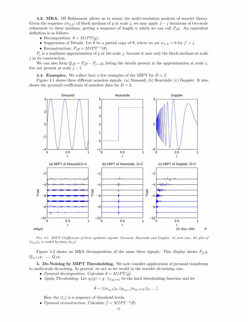
4.3. MRA. MI Refinement allows us to mimic the multi-resolution analysis of wavelet theory.Given the sequence (mj,k) of block medians of y at scale j, we may apply J − j iterations of two-scalerefinement to these medians, getting a sequence of length n which we can call Pjy. An equivalentdefinition is as follows:

• Decomposition: θ = MIPT (y).• Suppression of Details. Let θ be a partial copy of θ, where we set αj′,k = 0 for j′ > j.• Reconstruction: Pjy = MIPT−1(θ).

Pj is a nonlinear approximation of y at the scale j, because it uses only the block medians at scalej in its construction.

We can also form Qjy = Pjy − Pj−1y, listing the details present in the approximation at scale j,but not present at scale j − 1.

4.4. Examples. We collect here a few examples of the MIPT for D = 2.Figure 4.1 shows three different noiseless signals: (a) Sinusoid; (b) Heaviside; (c) Doppler. It also

shows the pyramid coefficients of noiseless data for D = 2.

0 0.5 1−4

−2

0

2

4

t

Sinusoid

0 0.5 1−10

−8

−6

−4

−2

t

Tria

d

(a) MIPT of Sinusoid,D=2

0 0.5 1−1

0

1

2

3

4

5

t

Heaviside

0 0.5 1−10

−8

−6

−4

−2

t

Tria

d

(b) MIPT of Heaviside, D=2

0 0.5 1−5

0

5

t

Doppler

0 0.5 1−10

−8

−6

−4

−2

t

Tria

d

(c) MIPT of Doppler, D=2

mifig41 23−Sep−1997 R

Fig. 4.1. MIPT Coefficients of three synthetic signals: Sinusoid, Heaviside and Doppler. In each case, the plot of(αj,k)k is scaled by maxk |αj,k|

Figure 4.2 shows an MRA decomposition of the same three signals. This display shows Pj0y,Qj0+1y, . . . , QJy.

5. De-Noising by MIPT Thresholding. We now consider applications of pyramid transformsto multi-scale de-noising. In general, we act as we would in the wavelet de-noising case.

• Pyramid decomposition. Calculate θ = MIPT (y).• Apply Thresholding. Let ηt(y) = y · 1{|y|>t} be the hard thresholding function and let

θ = ((mj0,k)k, (ηtj0+1(αj0+1,k))k, ....)

Here the (tj) is a sequence of threshold levels.• Pyramid reconstruction. Calculate f = MIPT−1(θ).

17

0 0.5 1−4

−2

0

2

4

t

Sinusoid

0 0.5 1−10

−8

−6

−4

−2

t

Tria

d

(a) MIPT of Sinusoid,D=2

0 0.5 1−1

0

1

2

3

4

5

t

Heaviside

0 0.5 1−10

−8

−6

−4

−2

t

Tria

d

(b) MIPT of Heaviside, D=2

0 0.5 1−5

0

5

t

Doppler

0 0.5 1−10

−8

−6

−4

−2

tT

riad

(c) MIPT of Doppler, D=2

mifig42 23−Sep−1997 R

Fig. 4.2. Nonlinear Multi-Resolution Analysis of three synthetic signals: Sinusoid, Heaviside and Doppler. ForHeaviside and Doppler, the plots of Qj are scaled the same for all j; whereas for the Sinusoid, each Qj is scaled bymaxk |(Qj)k|

In this approach, coefficient amplitudes smaller than tj are judged negligible, as noise rather thansignal. Hence the thresholds tj control the degree of noise rejection, but also of valid signal rejection.One hopes, in analogy with the orthogonal transform case studied in [12], to set thresholds which aresmall, but which are very likely to exceed every coefficient in case of a pure noise signal. If the MIPTperforms as we hope, the MIPT thresholds can be set ‘as if’ the noise were Gaussian and the transformwere AIPT, even when the noise is very non-Gaussian. This would mean that the median pyramid isimmune to bad effects of impulsive noise.

5.1. Choice of Thresholds. Motivated by P4 and P5, we work with the “L2-normalized” coef-ficients αj,k =

√3J−jαj,k in this section.

In order to choose thresholds {tj} which are very likely to exceed every coefficient in case of apure noise signal, we find tj satisfying P (|αj,k| > tj) ≤ c · 3−J/J where the MIPT coefficients arisefrom a pure noise signal (Xi)3J−1

i=0 , Xi ∼i.i.d. F . Then we have

P (∃(j, k) s.t. |αj,k| > tj) ≤ c ·J∑

j=j0

3j−1∑k=0

1J

3−J → 0 as J →∞.(5.1)

By (6.5), we can simply choose tj satisfying P (√

3J−j |med(X1, . . . , X3J−j )| > tj) ≤ 3−J/J . Corollary6.5 gives, when F is a symmetric law,

tj := tj(F ) =√

3J−jF−1

12

+12

√1−

(1

2J3J

) 23J−j

.(5.2)

Careful study of (5.2) suggests to us that away from the finest scales, the magnitude of tj isgoverned by the behavior of F−1 near 1/2. Hence after standardizing the level and slope of F atp = 1/2 we expect that the threshold depends very little on F .

18

To illustrate this, we define classes of smooth distributions standardized in this fashion. Weconsider distributions with densities f symmetric about 0, so that F−1(1/2) = 0. We standardizeunits so that for the distributions under consideration the density obeys f(0) = 1/

√2π, the same

as the standard Gaussian N(0, 1). This is of course equivalent to setting (F−1)′(1/2) =√

2π. Wealso impose on F−1(p) some regularity near p = 1/2: the existence of two continuous derivativesthroughout [1/2− η, 1/2 + η]. Our classes of symmetric distributions F(M,η) are then

F(M,η) := {F : f symmetric , (F−1)′(1/2) =√

2π, |(F−1)′′(p)| ≤M, |p− 1/2| ≤ η}

where M > 0 and 0 < η < 1/2 are absolute constants. The Appendix provesTheorem 5.1. For any ε > 0 and θ ∈ (0, 1), there exists J∗ = J∗(ε, θ,M, η) such that if J ≥ J∗

then

maxj≤bθJc

|tj(F1)− tj(F2)| ≤ ε, ∀F1, F2 ∈ F(M,η).

5.2. Alpha-Stable Laws. Theorem 5.1 shows that a single set of MIPT thresholds can worknot only for Gaussian data but also for a wide family of distributions – provided that we avoid theuse of coefficients at the finest scales. To illustrate the theorem, we consider symmetric α-stable laws(SαS) [25]. Alpha-stable laws are good models for many applications because of their high variability[22, 25].

Each symmetric α-stable law SαS is specified by its characteristic function exp(−σα|θ|α), withtwo parameters, (α, σ), α ∈ (0, 2], σ > 0. The case α = 2 is the Gaussian distribution with standarddeviation

√2σ and density function 1/(

√2π√

2σ) exp(−t2/(4σ2). The case α = 1 is the Cauchydistribution with density σ/(π(σ2 + t2)).

For our purposes, we consider SαS densities with σ calibrated so that the density at zero hasthe same value 1/

√2π as the standard Gaussian. We denote the density and distribution of a SαS

standardized in this way by fα and Fα respectively. Notice that

fα(t) =1

2π

∫ +∞

−∞e−iωte−σ

α|ω|αdω =1π

∫ ∞0

e−σαωα cos(ωt)dω(5.3)

and therefore fα(0) = 1σπ I(α) where I(α) =

∫∞0e−ω

α

dω. So fα is properly calibrated by choosing

σ = σα =√

2/π · I(α).(5.4)

It is clear from (5.3) that fα(t) is smooth; The Appendix proves the following:Lemma 5.2. Let 0 < α0 < 2. {Fα : α ∈ [α0, 2]} is a subset of a F(M,η) for appropriate M and

η.Combining this with Theorem 5.1 givesCorollary 5.3. For any ε > 0, θ ∈ (0, 1) and α0 ∈ (0, 2), there exists J∗ = J∗(ε, θ, α0) such

that if J ≥ J∗ then

maxj≤bθJc

|tj(Fα1)− tj(Fα2)| ≤ ε, ∀α0 ≤ α1, α2 ≤ 2.

To illustrate Corollary 5.3, we compare tj(F2) with tj(F1) in Table 5.1.While the Gaussian and Cauchy are widely different distributions, their MIPT thresholds are very

close at coarse scales.

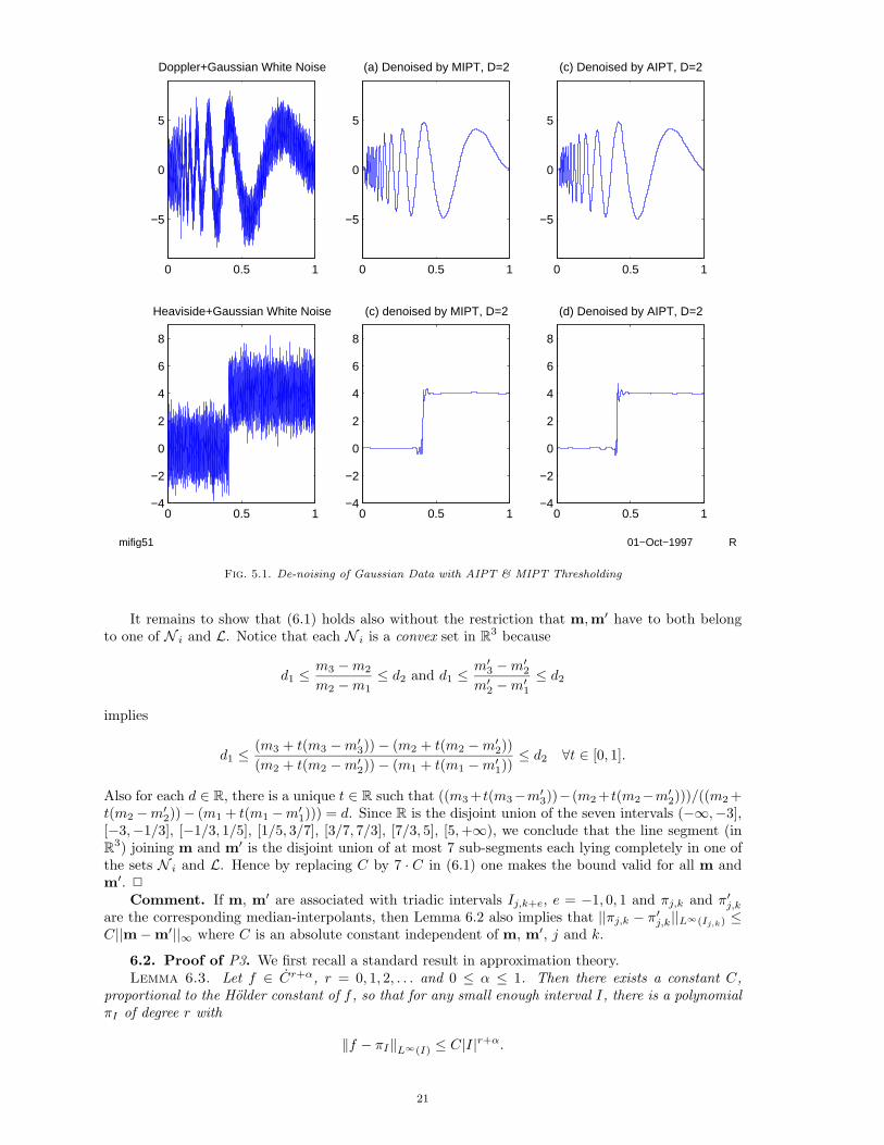
5.3. De-Noising in Gaussian Noise. In order to test the above ideas, we first report on thebehavior of MIPT with Gaussian noise. Figure 5.1 shows two objects – Heaviside and Doppler –contaminated by Gaussian noise.

The figure also shows the results for (a) Doppler signal, thresholding in MIPT domain; (b) Dopplersignal, thresholding in AIPT domain; (c) Heaviside signal, thresholding in MIPT domain; (d) Heavisidesignal, thresholding in AIPT domain.

The thresholds tj in both cases were set by (5.2). The performance of MIPT is comparable to theperformance of AIPT, as we expect.

19

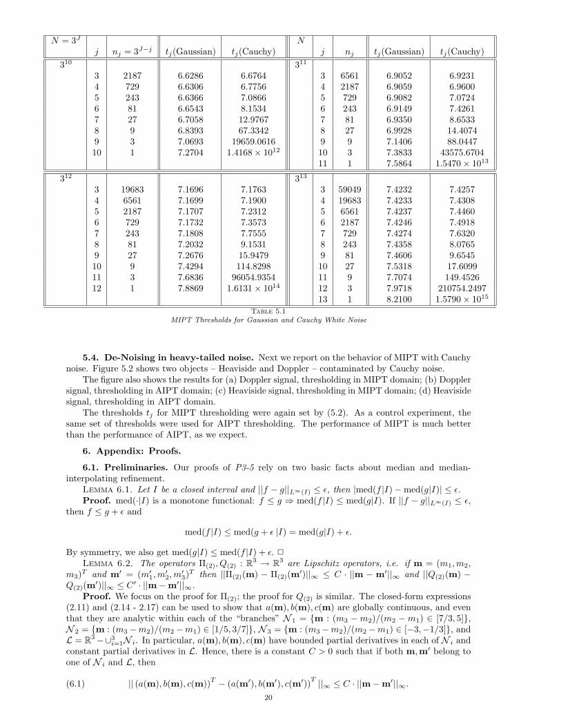
N = 3J Nj nj = 3J−j tj(Gaussian) tj(Cauchy) j nj tj(Gaussian) tj(Cauchy)

310 311

3 2187 6.6286 6.6764 3 6561 6.9052 6.92314 729 6.6306 6.7756 4 2187 6.9059 6.96005 243 6.6366 7.0866 5 729 6.9082 7.07246 81 6.6543 8.1534 6 243 6.9149 7.42617 27 6.7058 12.9767 7 81 6.9350 8.65338 9 6.8393 67.3342 8 27 6.9928 14.40749 3 7.0693 19659.0616 9 9 7.1406 88.044710 1 7.2704 1.4168× 1012 10 3 7.3833 43575.6704

11 1 7.5864 1.5470× 1013

312 313

3 19683 7.1696 7.1763 3 59049 7.4232 7.42574 6561 7.1699 7.1900 4 19683 7.4233 7.43085 2187 7.1707 7.2312 5 6561 7.4237 7.44606 729 7.1732 7.3573 6 2187 7.4246 7.49187 243 7.1808 7.7555 7 729 7.4274 7.63208 81 7.2032 9.1531 8 243 7.4358 8.07659 27 7.2676 15.9479 9 81 7.4606 9.654510 9 7.4294 114.8298 10 27 7.5318 17.609911 3 7.6836 96054.9354 11 9 7.7074 149.452612 1 7.8869 1.6131× 1014 12 3 7.9718 210754.2497

13 1 8.2100 1.5790× 1015

Table 5.1

MIPT Thresholds for Gaussian and Cauchy White Noise

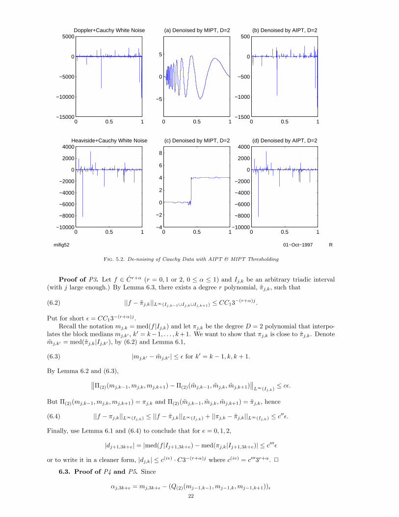
5.4. De-Noising in heavy-tailed noise. Next we report on the behavior of MIPT with Cauchynoise. Figure 5.2 shows two objects – Heaviside and Doppler – contaminated by Cauchy noise.

The figure also shows the results for (a) Doppler signal, thresholding in MIPT domain; (b) Dopplersignal, thresholding in AIPT domain; (c) Heaviside signal, thresholding in MIPT domain; (d) Heavisidesignal, thresholding in AIPT domain.

The thresholds tj for MIPT thresholding were again set by (5.2). As a control experiment, thesame set of thresholds were used for AIPT thresholding. The performance of MIPT is much betterthan the performance of AIPT, as we expect.

6. Appendix: Proofs.

6.1. Preliminaries. Our proofs of P3-5 rely on two basic facts about median and median-interpolating refinement.

Lemma 6.1. Let I be a closed interval and ||f − g||L∞(I) ≤ ε, then |med(f |I)−med(g|I)| ≤ ε.Proof. med(·|I) is a monotone functional: f ≤ g ⇒ med(f |I) ≤ med(g|I). If ||f − g||L∞(I) ≤ ε,

then f ≤ g + ε and

med(f |I) ≤ med(g + ε |I) = med(g|I) + ε.

By symmetry, we also get med(g|I) ≤ med(f |I) + ε. 2

Lemma 6.2. The operators Π(2), Q(2) : R3 → R3 are Lipschitz operators, i.e. if m = (m1,m2,m3)T and m′ = (m′1,m

′2,m

′3)T then ||Π(2)(m) − Π(2)(m′)||∞ ≤ C · ||m − m′||∞ and ||Q(2)(m) −

Q(2)(m′)||∞ ≤ C ′ · ||m−m′||∞.Proof. We focus on the proof for Π(2); the proof for Q(2) is similar. The closed-form expressions

(2.11) and (2.14 - 2.17) can be used to show that a(m), b(m), c(m) are globally continuous, and eventhat they are analytic within each of the “branches” N 1 = {m : (m3 −m2)/(m2 −m1) ∈ [7/3, 5]},N 2 = {m : (m3 −m2)/(m2 −m1) ∈ [1/5, 3/7]}, N 3 = {m : (m3 −m2)/(m2 −m1) ∈ [−3,−1/3]}, andL = R3−∪3

i=1N i. In particular, a(m), b(m), c(m) have bounded partial derivatives in each of N i andconstant partial derivatives in L. Hence, there is a constant C > 0 such that if both m,m′ belong toone of N i and L, then

|| (a(m), b(m), c(m))T − (a(m′), b(m′), c(m′))T ||∞ ≤ C · ||m−m′||∞.(6.1)20

0 0.5 1

−5

0

5

Doppler+Gaussian White Noise

0 0.5 1−4

−2

0

2

4

6

8

Heaviside+Gaussian White Noise

0 0.5 1

−5

0

5

(a) Denoised by MIPT, D=2

0 0.5 1−4

−2

0

2

4

6

8

(c) denoised by MIPT, D=2

0 0.5 1

−5

0

5

(c) Denoised by AIPT, D=2

0 0.5 1−4

−2

0

2

4

6

8

(d) Denoised by AIPT, D=2

mifig51 01−Oct−1997 R

Fig. 5.1. De-noising of Gaussian Data with AIPT & MIPT Thresholding

It remains to show that (6.1) holds also without the restriction that m,m′ have to both belongto one of N i and L. Notice that each N i is a convex set in R3 because

d1 ≤m3 −m2

m2 −m1≤ d2 and d1 ≤

m′3 −m′2m′2 −m′1

≤ d2

implies

d1 ≤(m3 + t(m3 −m′3))− (m2 + t(m2 −m′2))(m2 + t(m2 −m′2))− (m1 + t(m1 −m′1))

≤ d2 ∀t ∈ [0, 1].

Also for each d ∈ R, there is a unique t ∈ R such that ((m3 + t(m3−m′3))−(m2 + t(m2−m′2)))/((m2 +t(m2 −m′2))− (m1 + t(m1 −m′1))) = d. Since R is the disjoint union of the seven intervals (−∞,−3],[−3,−1/3], [−1/3, 1/5], [1/5, 3/7], [3/7, 7/3], [7/3, 5], [5,+∞), we conclude that the line segment (inR3) joining m and m′ is the disjoint union of at most 7 sub-segments each lying completely in one ofthe sets N i and L. Hence by replacing C by 7 · C in (6.1) one makes the bound valid for all m andm′. 2

Comment. If m, m′ are associated with triadic intervals Ij,k+e, e = −1, 0, 1 and πj,k and π′j,kare the corresponding median-interpolants, then Lemma 6.2 also implies that ||πj,k − π′j,k||L∞(Ij,k) ≤C||m−m′||∞ where C is an absolute constant independent of m, m′, j and k.

6.2. Proof of P3. We first recall a standard result in approximation theory.Lemma 6.3. Let f ∈ Cr+α, r = 0, 1, 2, . . . and 0 ≤ α ≤ 1. Then there exists a constant C,

proportional to the Holder constant of f , so that for any small enough interval I, there is a polynomialπI of degree r with

‖f − πI‖L∞(I) ≤ C|I|r+α.

21

0 0.5 1−15000

−10000

−5000

0

5000Doppler+Cauchy White Noise

0 0.5 1−10000

−8000

−6000

−4000

−2000

0

2000

4000Heaviside+Cauchy White Noise

0 0.5 1

−5

0

5

(a) Denoised by MIPT, D=2

0 0.5 1−4

−2

0

2

4

6

8

(c) Denoised by MIPT, D=2

0 0.5 1−1500

−1000

−500

0

500(b) Denoised by AIPT, D=2

0 0.5 1−10000

−8000

−6000

−4000

−2000

0

2000

4000(d) Denoised by AIPT, D=2

mifig52 01−Oct−1997 R

Fig. 5.2. De-noising of Cauchy Data with AIPT & MIPT Thresholding

Proof of P3. Let f ∈ Cr+α (r = 0, 1 or 2, 0 ≤ α ≤ 1) and Ij,k be an arbitrary triadic interval(with j large enough.) By Lemma 6.3, there exists a degree r polynomial, πj,k, such that

||f − πj,k||L∞(Ij,k−1∪Ij,k∪Ij,k+1) ≤ CC13−(r+α)j .(6.2)

Put for short ε = CC13−(r+α)j .Recall the notation mj,k = med(f |Ij,k) and let πj,k be the degree D = 2 polynomial that interpo-

lates the block medians mj,k′ , k′ = k−1, . . . , k+ 1. We want to show that πj,k is close to πj,k. Denotemj,k′ = med(πj,k|Ij,k′), by (6.2) and Lemma 6.1,

|mj,k′ − mj,k′ | ≤ ε for k′ = k − 1, k, k + 1.(6.3)

By Lemma 6.2 and (6.3),∥∥Π(2)(mj,k−1,mj,k,mj,k+1)−Π(2)(mj,k−1, mj,k, mj,k+1)∥∥L∞(Ij,k)

≤ cε.

But Π(2)(mj,k−1,mj,k,mj,k+1) = πj,k and Π(2)(mj,k−1, mj,k, mj,k+1) = πj,k, hence

||f − πj,k||L∞(Ij,k) ≤ ||f − πj,k||L∞(Ij,k) + ||πj,k − πj,k||L∞(Ij,k) ≤ c′′ε.(6.4)

Finally, use Lemma 6.1 and (6.4) to conclude that for e = 0, 1, 2,

|dj+1,3k+e| = |med(f |Ij+1,3k+e)−med(πj,k|Ij+1,3k+e)| ≤ c′′′ε

or to write it in a cleaner form, |dj,k| ≤ c(iv) · C3−(r+α)j where c(iv) = c′′′3r+α. 2

6.3. Proof of P4 and P5. Since

αj,3k+ε = mj,3k+ε − (Q(2)(mj−1,k−1,mj−1,k,mj−1,k+1))ε22

and Q(2) is Lipschitz (Lemma 6.2), there is a constant c > 0, independent of j and k, such that|αj,3k+ε| ≤ c ·max(|mj,3k+ε|, |mj−1,k−1|, |mj−1,k|, |mj−1,k+1|). Boole’s inequality gives for random vari-ables Wi that

P (max(W1, . . . ,W4) > ξ) ≤4∑i=1

P (Wi > ξ)

and so we can write

P (√

3J−j |αj,k| ≥ ξ) ≤ 4 · P (√

3J−j |mj,k| ≥ ξ/c).(6.5)

Thus, P4 and P5 boil down to the calculation of P (√n|med(X1, . . . , Xn)| ≥ ξ) for Xi ∼i.i.d. Gaussian

and Cauchy.We first develop an inequality which derives from standard results in order statistics [6] and in

Cramer-Chernoff bounds on large deviations [7].Lemma 6.4. Let X1, . . . , Xn be i.i.d. with c.d.f. F (·). We have the following estimate:

P (|med(X1, . . . , Xn)| ≥ x) ≤ min{

1,[2√F (x)(1− F (x))

]n+[2√F (−x)(1− F (−x))

]n}.

Proof. It suffices to show that P (med(X1, . . . , Xn) ≥ x) ≤[2√F (x)(1− F (x))

]nfor any x ≥ 0.

Let Ii = 1(Xi≥x),

P (med(X1, . . . , Xn) ≥ x) ≤ P(

n∑i=1

Ii ≥n

2

).

Since Ii ∼i.i.d. Bin(1, 1− F (x)), Sn :=∑ni=1 Ii ∼ Bin(n, 1− F (x)). By 1(Sn≥n2 ) ≤ eλSne−λ

n2 ∀λ > 0,

we have

P (Sn ≥n

2) ≤ min

λ>0E(eλSne−λ

n2 ) = min

λ>0e−λ

n2 E(eλ

∑ n1 Ii)

= minλ>0

e−λn2(F (x) + (1− F (x))eλ

)n=[minλ>0

F (x)e−λ2 + (1− F (x))e

λ2

]n=(F (x)e−

λ2 + (1− F (x))e

λ2 |λ=ln( F (x)

1−F (x) )

)n=(

2√F (x)(1− F (x))

)n. 2

Corollary 6.5. Let X1, . . . , Xn be i.i.d. with c.d.f. F (x) having symmetric density f . Givenα ∈ (0, 1/2), define

tα,n := F−1

(12

+12

√1−

(α2

) 2n

),

then

P (|med(X1, . . . , Xn)| ≥ tα,n) ≤ α.

We now apply Lemma 6.4 to the Gaussian and Cauchy distribution. Since they are both symmetricdistributions, we have

P(∣∣√n med(X1, . . . , Xn)

∣∣ ≥ ξ) ≤ 2 · 2n√F

(ξ√n

)(1− F

(ξ√n

))n

= 2 ·(

[4F (y) (1− F (y))]y−2/2

)ξ2

= 2 · exp(θ(y)ξ2)

where y ≡ ξ/√n and θ(y) ≡ y−2/2 · log [4F (y) (1− F (y))]. Gaussian-type probability bounds follow

for a range 0 ≤ ξ ≤ X in P4 and P5, if we show that sup[0,Y ] θ(y) < 0 on a corresponding range ofvalues 0 ≤ y ≤ Y .

23

(i) Gaussian Distribution : To establish P4, we need inequalities valid for 0 ≤ ξ < ∞, i.e.0 ≤ y <∞. Now

supy∈[2,∞)

θ(y) = supy∈[2,∞)

y−2/2 · [log(1− F2(y)) + log(4F2(y))] .

From Mills’ ratio∫∞ye−x

2/2dx ≤ 1y e−y2/2 holding ∀y > 1, we have log(1 − F2(y)) ≤ −y2/2 − log(y).

Hence

supy∈[2,∞)

θ(y) ≤ supy∈[2,∞)

y−2/2 ·[−y2/2− log(y) + log(4)

]= −(2− log(2))/2 < 0.

On the other hand, from symmetry of F2 and unimodality of the density f2 we get 4F2(y)(1−F2(y)) =4F2(y)F2(−y) ≤ 1− cy2 on |y| ≤ 2, with c > 0; so

supy∈[0,2]

θ(y) = supy∈[0,2]

y−2/2 · log(1− cy2) ≤ −c/2.

(ii) Cauchy Distribution: F1(x) = 12 + 1

πarctan(√

π2x). To get P5 we aim only for an inequality

valid on y ∈ [0, Y ], with Y = 1, which gives a Gaussian-type inequality for ξ ∈ [0,√n].

θ(y) = y−2/2 · log[1− 4

π2arctan2

(√π

2y

)]≤ −y−2/2 · 4

π2arctan2

(√π

2y

).

However, as arctan(y) > c · y for y ∈ [0, 1], with c > 0, this gives θ(y) < − c2π for y ∈ [0, 1].

6.4. Proof of Theorem 5.1. Let p = 1/(2J3J)2, nj = 3J−j . Let j be chosen such that

1/2√

1− p1/nj ≤ η.(6.6)

Then there exist 0 < η1, η2 ≤ η such that

|tj(F1)− tj(F2)| = √nj∣∣∣∣F−1

1

(12

+12

√1− p

1nj

)− F−1

2

(12

+12

√1− p

1nj

)∣∣∣∣=√nj∣∣(F−1

1 )′′(1/2 + η1)− (F−12 )′′(1/2 + η2)

∣∣ (12

√1− p

1nj

)2

≤M/2√nj

(1− p

1nj

),

i.e. |tj(F1)− tj(F2)| ≤ ε if

√nj

(1− p

1nj

)≤ 2εM.(6.7)

Since (1− x) ≤ log(1/x) ∀x ∈ (0, 1], (6.6) holds for large enough J because

12

√1− p1/nj ≤ 1

2

√log p−1/nj =

12

√1nj

log(4 · J2 · 32J)

≤ 12

√1

3(1−θ)J (log(4) + 2 log(J) + 2J log(3))→ 0 as J → 0.

Similarly, (6.7) holds for large enough J because

√nj

(1− p

1nj

)≤ (1/

√nj) log p−1

≤ 1√3(1−θ)J

(log(4) + 2 log(J) + 2J log(3))→ 0 as J → 0.2

24

6.5. Proof of Lemma 5.2. It suffices to find M, η such that

supα∈[α0,2]

supp∈[ 1

2−η,12 +η]

(F−1α )′′(p) ≤M.

Since

(F−1α )′′(p) = − f ′α(F−1

α (p))[fα(F−1

α (p))]3,

we work with F−1α , fα and f ′α separately.

1. Since |F−1α (p)| is monotone increasing in p for fixed α, and is monotone increasing in α for fixed

p, we have, for any 0 < η < 1/2 ,

sup0<α≤2

sup1/2−η≤p≤1/2+η

|F−1α (p)| = F−1

2 (1/2 + η).

2. Now sup|t|≤ε1 |fα(t)− fα(0)| ≤ |t| · {sup|t|≤ε1 |f ′α(t)|}. Also

sup|t|≤ε1

|f ′α(t)| = sup|t|≤ε1

∣∣∣∣ 1π∫ ∞

0

e−σααω

α

(−ω) sin(ωt)dω∣∣∣∣

≤ 1π

∫ ∞0

e−σααω

α

ωdω =1π

1σ2α

∫ ∞0

e−ωα

ωdω ≤ C1(α0)

where C1(α) = 12 (∫∞

0e−ω

α

ωdω)/(∫∞

0e−ω

α

dω)2 is defined on (0, 2] and is positive and monotonedecreasing.

3. Similarly sup|t|≤ε1 |f ′α(t)− f ′α(0)| ≤ |t| · {sup|t|≤ε1 |f ′′α(t)|}. Moreover

sup|t|≤ε1

|f ′′α(t)| = sup|t|≤ε1

∣∣∣∣ 1π∫ ∞

0

e−σααω

α

(ω2) cos(ωt)dω∣∣∣∣

≤ 1π

∫ ∞0

e−σααω

α

ω2dω =1π

1σ3α

∫ ∞0

e−ωα

ω2dω ≤ C2(α0)

where C2(α) = 12

√π2 (∫∞

0e−ω

α

ω2dω)/(∫∞

0e−ω

α

dω)3 is defined on (0, 2] and is positive and monotonedecreasing. Therefore

supα∈[α0,2]

supp∈[ 1

2−η,12 +η]

|(F−1α )′′(p)| = sup

α∈[α0,2]

supp∈[ 1

2−η,12 +η]

|f ′α(F−1α (p))|

|fα(F−1α (p))|3

≤|F−1

2 ( 12 + η)|C2(α0)∣∣∣ 1√

2π− F−1

2 ( 12 + η)C1(α0)

∣∣∣3 .(6.8)

If we choose η = η(α0) > 0 small enough such that F−12 ( 1

2 + η)C1(α0) < 1√2π

, then with the choice ofM = M(α0) defined by (6.8) we get {Fα : α0 ≤ α ≤ 2} ⊂ F(M(α0), η(α0)). 2

Reproducible Research. In this paper, all computational results are reproducible, meaning thatthe code which generated the figures is available over the Internet, following the discipline indicatedin [3]. Interested readers are directed to:http://stat.stanford.edu/~donoho/repro/median.html

Ackowledgements. This research was partially supported by NSF DMS-95-05151, by AFOSRMURI95-F49620-96-1-0028, and by other sponsors. The authors would like to thank Andrew Bruce,Amir Dembo, Gary Hewer, and Charles Micchelli for helpful discussions and references.

REFERENCES

[1] B.H. Borden and M.L. Mumford. A statistical glint/radar cross section target model. IEEE Trans. Aerosp. Elect.Sys., 19:781–785, 1983.

[2] Andrew G. Bruce, David L. Donoho, Hong-Ye Gao, and R. Douglas Martin. Denoising and robust nonlinear waveletanalysis. In SPIE Proceedings, Wavelet Applications, volume 2242, Orlando, FL, April 1994.

[3] J. Buckheit and D. L. Donoho. Wavelab and reproducible research. In A. Antoniadis and G. Oppenheim, editors,Wavelets in Statistics, pages 55–82. Springer-Verlag, 1994.

25

[4] I. Daubechies. Ten Lectures on Wavelets. Number 61 in CBMS-NSF Series in Applied Mathematics. SIAM,Philadelphia, 1992.

[5] I. Daubechies and J. Lagarias. Two-scale difference equations II. local regularity, infinite products of matrices andfractals. SIAM J. Math. Anal., 23(4):1031–1079, 1992.

[6] H. A. David. Order statistics. Wiley, 1970.

[7] A. Dembo and O. Zeitouni. Large Deviations and Applications. Bartlett and Jones, 1993.

[8] G. Deslauriers and S. Dubuc. Symmetric iterative interpolation processes. Constr. Approx., 5:49–68, 1989.

[9] D. L. Donoho. Interpolating wavelet transforms. Technical report, Department of Statistics, Stanford University,1992. Available at ftp://stat.stanford.edu/reports/donoho/interpol.ps.Z.

[10] D. L. Donoho. Smooth wavelet decompositions with blocky coefficient kernels. In L.L. Schumaker and G. Webb,editors, Recent Advances in Wavelet Analysis, pages 259–308. Boston: Academic Press, 1993.

[11] D. L. Donoho. Minimum entropy segmentation. In C.K. Chui, L. Montefusco, and L. Puccio, editors, WaveletsTheory, Algorithms and Applications, pages 233–269. Academic Press, 1994.

[12] D. L. Donoho. De-noising by soft-thresholding. IEEE Trans. on Information Theory., 41(3):613–27, 1995.

[13] D. L. Donoho and I. M. Johnstone. Adapting to unknown smoothness by wavelet shrinkage. J. Amer. Stat. Assn.,90:1200–1224, 1995.

[14] D. L. Donoho, I. M. Johnstone, G. Kerkyacharian, and D. Picard. Wavelet shrinkage: Asymptopia? J. Roy. Stat.Soc. Ser. B, 57:301–369, 1995.

[15] N. Dyn, J. Gregory, and D. Levin. Analysis of uniform binary subdivision schemes for curve design. Constr.Approx., 7:127–147, 1991.

[16] H.-Y. Gao. Wavelet estimation of spectral densities in time series analysis. PhD thesis, Department of Statistics,University of California, Berkeley, 1993.

[17] D.R. Greer, I. Fung, and J.H. Shapiro. Maximum-likelihood multiresolution laser radar range imaging. IEEETrans. Image Proc., 6:36–47, 1997.

[18] P. Hall and P. Patil. On the choice of smoothing parameter, threshold and truncation in nonparametric regressionby wavelet methods. J. Roy. Stat. Soc. Ser. B, 58:361–377, 1996.

[19] F. R. Hampel. Robust Statistics: the approach based on influence functions. Wiley, 1986.

[20] P. Huber. Robust Statistics. Wiley, 1981.

[21] H. Longbotham. A class of robust nonlinear filters for signal decomposition and filtering utilizing the Haar basis.In ICASSP-92, volume 4. IEEE Signal Processing Society, March 1992.

[22] C. L. Nikias and M. Shao. Signal Processing with Alpha-Stable Distributions and Applications. Wiley, 1995.

[23] O. Rioul. Simple regularity criteria for subdivision schemes. SIAM J. Math. Anal., 23(6):1544–1576, November1992.

[24] D.A. F. Florencio R.L. de Queiroz and R.W. Schafer. Nonexpansive pyramid for image coding using a non-linearfilter bank. IEEE Trans. Image Proc., page to appear, 1998.

[25] G. Samorodnitsky and M. S. Taqqu. Stable Non-Gaussian Random Process: Stochastic Models with InfiniteVariance. Chapman & Hall, 1994.

[26] J.L. Starck. Astronomical image compression using the pyramid median transform. Manuscript.CEA/DSM/DAPNIA Gif Sur Yvette., 1995.

[27] J.L. Starck, F. Murtagh, B. Pirenne, and M. Albrecht. Astronomical image compression based on noise suppression.Proc. Astro. Soc. Pac., 108:446–455, 1996.

[28] B.W. Stuck and B. Kleiner. A statistical analysis of telephone noise. Bell Syst. Tech. J., 53:1263–1320, 1974.

[29] T. P.-Y. Yu. New Developments in Interpolating Wavelet Transforms. PhD thesis, Program of Scientific Computingand Computational Mathematics, Stanford University, August 1997.

26