tspace.library.utoronto.ca wave propagation behaviour in symmetric and non-symmetric...
TRANSCRIPT
Wave Propagation Behaviour in Symmetric and Non-symmetricThree-dimensional Lattice Structures for Tailoring the Band Gaps
by
Jaehoon Won
A thesis submitted in conformity with the requirementsfor the degree of Master of Applied Science
Graduate Department of Aerospace Science and EngineeringUniversity of Toronto
c© Copyright 2016 by Jaehoon Won
Abstract
Wave Propagation Behaviour in Symmetric and Non-symmetric Three-dimensional Lattice Structures
for Tailoring the Band Gaps
Jaehoon Won
Master of Applied Science
Graduate Department of Aerospace Science and Engineering
University of Toronto
2016
In this thesis, the longitudinal flexural wave propagation behaviour through symmetric and non-symmetric
tetrahedral and pyramidal lattice structures is analyzed. Finite element analysis employing Floquet-
Bloch theory is used to generate and plot dispersion curves. The design variables of the lattice structures
are modified to analyze their impact on the dispersion curves. In symmetric lattice structures, changes in
stiffness and density provide the effect of scaling the dispersion curves, whereas in non-symmetric lattice
structures, based on the location of the inhomogeneities applied, asymmetric dispersion relations are ob-
tained. For systems in which only certain directions of wave propagation are considered, non-symmetric
lattice structures and the resulting asymmetric dispersion relations demonstrate great strength in terms
of their flexibility when tailoring dispersion curves, as a large number of directionally different dispersion
curves can be obtained, providing more options to design and optimize the lattice structure. Critically,
band gaps can be designed at desirable frequencies and directions.
ii

Acknowledgements
I would like to thank my supervisor Dr. Craig A. Steeves, for his support, trust, and guidance through-
out the duration of the Master’s program. It was invaluable opportunity and experience to work with
him. Secondly, I wish to thank my RAC advisors, Dr. David W. Zingg, Dr. Phillippe Lavoie, Dr.
Prasanth B. Nair and Dr. Alis Ekmekci for their instructions and constructive feedback throughout the
Master’s program. Thirdly, I wish to thank Manan Arya, former student who had worked on the topic
of wave propagation in periodic lattice structure, for allowing his initial work on numerical models and
his research to be used as back bone structure, being great guidance of initiating this Master’s research.
Special thank to my family for endless support on pursuing my goal, allowing me to be able to focus on
the research without being interrupted by any obstacles. Lastly, I would like to thank Bharat Bhaga,
David Platt, Nick Ewaschuk, and Qian Zhang, the colleagues in the Multifunctional Structures Lab
of University of Toronto Institute for Aerospace Studies, for their support and feedback, and making
studying environment to be full of enjoyment.
Jaehoon Won
University of Toronto Institute for Aerospace Studies
iii
Contents
1 Introduction 1
1.1 Motivation: Design for Sustainable Aviation . . . . . . . . . . . . . . . . . . . . . . . . . . 1
1.2 Literature Review . . . . . . . . . . . . . . . . . . . . . . . . . . . . . . . . . . . . . . . . 3
1.2.1 Nanocrystalline Metals . . . . . . . . . . . . . . . . . . . . . . . . . . . . . . . . . . 3
1.2.2 Electrodeposition Processing . . . . . . . . . . . . . . . . . . . . . . . . . . . . . . 3
1.2.3 Lattice Structure . . . . . . . . . . . . . . . . . . . . . . . . . . . . . . . . . . . . . 3
1.3 Wave Propagation in Two-dimensional Periodic Lattices . . . . . . . . . . . . . . . . . . . 4
1.4 Project Scope . . . . . . . . . . . . . . . . . . . . . . . . . . . . . . . . . . . . . . . . . . . 6
1.5 Outline of the Thesis Structure . . . . . . . . . . . . . . . . . . . . . . . . . . . . . . . . . 7
2 Periodic Lattice Structures 8
2.1 Generating Physical Lattice Structures . . . . . . . . . . . . . . . . . . . . . . . . . . . . . 8
2.2 Direct Lattice Structures in the Wave Space: Reciprocal Lattices . . . . . . . . . . . . . . 11
2.3 Properties and Behaviour of Wave Propagation in an Infinite Lattice Structure . . . . . . 13
2.3.1 Brillouin Zone in a Reciprocal Lattice . . . . . . . . . . . . . . . . . . . . . . . . . 13
2.3.2 Floquet and Bloch Theorem . . . . . . . . . . . . . . . . . . . . . . . . . . . . . . . 14
2.3.3 Coated Polymer Lattice Structure: An Ultralight Structure . . . . . . . . . . . . . 14
3 Finite Element Analysis 16
3.1 Defining the Input Parameters . . . . . . . . . . . . . . . . . . . . . . . . . . . . . . . . . 16
3.2 Defining the Mesh Size and Meshed Elements . . . . . . . . . . . . . . . . . . . . . . . . . 17
3.3 Defining the Nodes of the Structure . . . . . . . . . . . . . . . . . . . . . . . . . . . . . . 18
3.4 Defining Direct Basis Vectors and Reciprocal Basis Vectors . . . . . . . . . . . . . . . . . 20
3.5 Defining the Brillouin Zone . . . . . . . . . . . . . . . . . . . . . . . . . . . . . . . . . . . 21
3.6 Defining Eigenvalue Problems . . . . . . . . . . . . . . . . . . . . . . . . . . . . . . . . . . 21
3.6.1 Timoshenko Beams and Nodal Displacements . . . . . . . . . . . . . . . . . . . . . 21
3.7 Setting up the Shape Functions . . . . . . . . . . . . . . . . . . . . . . . . . . . . . . . . . 22
3.8 Kinetic Energy of a Timoshenko Beam: Setting the Local Mass Matrix . . . . . . . . . . . 24
3.9 Strain Potential Energy of a Timoshenko Beam: Setting the Local Stiffness Matrix . . . . 29
3.10 Evaluating the Shape Functions Involved in the Mass and Stiffness Matrices . . . . . . . . 33
3.11 Construction of the Local and Global Mass and Stiffness Matrices . . . . . . . . . . . . . 34
3.12 Obtaining the Equation of Motion . . . . . . . . . . . . . . . . . . . . . . . . . . . . . . . 36
iv

4 Wave propagation analysis 41
4.1 Plotting Dispersion Curves . . . . . . . . . . . . . . . . . . . . . . . . . . . . . . . . . . . 41
4.2 Modifying the Design Variables to Tailor the Dispersion Curve . . . . . . . . . . . . . . . 42
4.3 Properties of Dispersion Curves . . . . . . . . . . . . . . . . . . . . . . . . . . . . . . . . . 44
4.3.1 Velocity of Wave Propagation . . . . . . . . . . . . . . . . . . . . . . . . . . . . . . 44
4.3.2 Dispersion Branches, Veering Effect and Natural Frequencies . . . . . . . . . . . . 44
4.3.3 Band Gap Phenomenon . . . . . . . . . . . . . . . . . . . . . . . . . . . . . . . . . 47
4.4 Validation Through Two-dimensional Triangular Lattices . . . . . . . . . . . . . . . . . . 47
4.5 Gaining a Physical Understanding of the Lattice Structure . . . . . . . . . . . . . . . . . . 49
4.6 Wave Propagation Through a Tetrahedral Lattice Structure with a Radius to Length
Ratio of 0.1 . . . . . . . . . . . . . . . . . . . . . . . . . . . . . . . . . . . . . . . . . . . . 50
4.6.1 Initial Symmetric Lattice Structure . . . . . . . . . . . . . . . . . . . . . . . . . . . 50
4.6.2 Impact of Changing the Design Variables E and ρ for All the Struts of the Lattice
Structure . . . . . . . . . . . . . . . . . . . . . . . . . . . . . . . . . . . . . . . . . 53
4.6.3 Impact of Changing the Design Variables E and ρ for a Non-Symmetric Lattice
Structure . . . . . . . . . . . . . . . . . . . . . . . . . . . . . . . . . . . . . . . . . 57
4.6.4 Impact of Modifying Different Combinations of Struts of the Lattice Structure . . 65
4.6.5 Impact of Increasing the Number of Struts Being Modified . . . . . . . . . . . . . 70
4.6.6 Intuitive and Physical Understanding of the Dispersion Relations of a Non-Symmetric
Lattice Structure . . . . . . . . . . . . . . . . . . . . . . . . . . . . . . . . . . . . . 74
4.6.7 Significance of the Asymmetric Dispersion Relations . . . . . . . . . . . . . . . . . 76
4.6.8 Impact of Changing the Other Design Variables . . . . . . . . . . . . . . . . . . . . 76
5 Conclusion and Future Recommendations 81
5.1 Conclusion . . . . . . . . . . . . . . . . . . . . . . . . . . . . . . . . . . . . . . . . . . . . 81
5.2 Future Recommendations . . . . . . . . . . . . . . . . . . . . . . . . . . . . . . . . . . . . 83
5.2.1 Multi-Tetrahedral/Pyramidal Non-Symmetric Unit Cell . . . . . . . . . . . . . . . 83
5.2.2 Shape Shifting Lattice Structure . . . . . . . . . . . . . . . . . . . . . . . . . . . . 85
5.2.3 Lattice Structure as the Core of Sandwich Panel . . . . . . . . . . . . . . . . . . . 86
Bibliography 87
v

Chapter 1
Introduction
1.1 Motivation: Design for Sustainable Aviation
Air transport has experienced rapid expansion as the global economy has grown and the technology
of air transport has developed to its present state. However, with the expected increase in global air
travel over the next 30 years, the reliability and environmental impact of aviation are becoming critical
issues for the future of flight. Without significant action, large economic and environmental impacts are
expected. Sustainable aviation is the initiative to prevent or reduce the expected economic and envi-
ronmental impacts of aviation. The goal of designing for sustainable aviation is to develop technologies
that will allow a tripling of capacity yet at the same time with a reduction in environmental impact.
The following are the main areas where work is focused to achieve sustainable aviation:
1. Source noise reduction;
2. Source emissions reduction;
3. Materials and manufacturing processes;
4. Airport operations;
5. Aircraft operations;
6. Alternative fuels;
7. Product lifecycle management.
Recently, light weight structures that can be used in various engineering applications have been a focus
of research and development. Metallic foams, a cellular structure consisting of a solid metal filled with
gas bubbles with 75% to 95% of the volume void space, have been one of the competing ultralight ma-
terials. However, Hutchinson and Fleck [13] state that because the cell walls deform by local bending,
the mechanical properties of metallic foam are poor. This led to a search for stretch-dominant open-cell
microstructures, such as periodic lattices, which give much higher stiffness and strength per unit mass
than foams. For example, when an octet-truss lattice structure is compared with metallic foam, the stiff-
ness and strength of the lattice material exceeds the corresponding values for metal foams by a factor
of between 3 and 10 [8]. Indeed, due to a high strength-to-weight ratio, relative ease of manufacture,
and potential for multifunctional applications, lattice structures are an attractive alternative to metallic
foams.
1

Chapter 1. Introduction 2
Figure 1.1: Illustration of a bending-dominant structure versus a stretch-dominant structure from Desh-pande et al. [8].
As Figure 1.1 illustrates, when force is applied at the top and bottom corner of a bending-dominant
structure, the struts can rotate around each pin-joint, potentially leading to the structure to collapse.
However, when force is applied at the same location for a stretch-dominant structure, an additional strut
placed in the centre can support the applied forces through tension and compression in the other struts,
keeping the structure intact [6].
Previously at the University of Toronto Institute for Aerospace and Studies (UTIAS), Arya and Steeves
[1] developed a numerical model of wave propagation behaviour in three-dimensional (3D) lattice struc-
tures. The goal of this thesis is to explore this numerical model and to construct new algorithms for a
deeper analysis and comparison of various 3D lattice structures that have a tailorable structural stiffness
and strength, together with capability to preventing vibrations at undesirable frequency ranges.
The first goal of the research therefore is to improve the performance of light-weight 3D lattice struc-
tures in terms of their tailorable structural strength, stiffness, and band gaps. Achieving this goal will
contribute to sustainable aviation by improving fuel efficiency, which will be enhanced by reducing the
overall weight of the plane through the use of such lightweight structures. The second goal of the research
is to investigate how the band gaps can be engineered to appear in the desirable frequency range, such
that there will be no vibration within the band gaps. Preventing the vibration by introducing the band
gaps in a certain frequency range is another potential contribution towards sustainable aviation as this
knowledge could be used in developing frequency filters in noise filters or in vibration protection materi-
als or devices aimed at reducing aircraft noises due to sound or vibration. The final goal of the research
is to apply inhomogeneities into the lattice structures, changing the lattice structures from symmetric to
non-symmetric lattice structures, with the purpose of analyzing the differences in the wave propagation
behaviour and the resulting dispersion curves between symmetric and non-symmetric lattice structures.
This will assist exploring the advanced approaches that will allow easier and flexible tailoring of the
lattice structures and band gaps.

Chapter 1. Introduction 3
1.2 Literature Review
1.2.1 Nanocrystalline Metals
Gleiter [11] presented a comprehensive overview of nanocrystalline materials. Nanocrystalline mate-
rials have characteristic length scales of nanometres, which endows them with unique microstructure-
dependent properties. Most properties of solids depend on their microstructural features, such as their
chemical composition, arrangement of the atoms, and grain size. Two solids composed of exactly the
same atoms may show differences in their solid properties if there are differences in their microstruc-
tures. One example of this, for instance, is the difference in the solid properties between diamond and
graphite. Diamond contains carbon atoms arranged tetrahedrally in three dimensions, while graphite
contains carbon atoms arranged hexagonally in two dimensions, a planar layered structure. Due to this
difference in atomic arrangement, diamond has a higher strength, hardness, and density than graphite.
Nanocrystalline materials can also attain new properties through a controlled manipulation of their
microstructural parameters at the grain size level. This enables new nanocrystalline materials to gain
better material properties and performances, such as ultra-high yields and fracture strengths, decreased
elongation and toughness, and superior wear resistance according to Kumar et al. [14]. For example,
the Hall-Petch effect [19] states that plastic deformation occurs more rapidly with larger grain sizes, and
the yield strength rises as the grain size decreases, which implies that nanocrystalline materials can have
an ultra-high yield strength.
1.2.2 Electrodeposition Processing
Kumar et al. [14] presented four methods of laboratory-scale processing applicable to metals or alloys
in different grain size ranges: 1) mechanical alloying and compaction, 2) severe plastic deformation, 3)
gas-phase condensation of the particulates, followed by consolidation and 4) electrodeposition. While the
first two methods are applied to yield ultrafine but not nanocrystalline materials, the last two methods
yield nanocrystalline materials. Electrodeposition, which is capable of producing material with a mean
grain size in the tens of nanometres, has so far been used for two major purposes: to produce sheets
of nanocrystalline metals (such as Ni, Co, Cu) and to produce binary alloys (such as Ni-Fe and Ni-W),
in which the grain size can be controlled to produce nanocrystalline metal coatings on complex shapes.
Electrodeposition is well-suited to depositing nanocrystalline metals with high accuracy onto complex
lattice preforms of various solid materials, such as metal alloys or polymers at the micrometre length
scale [28, 27].
1.2.3 Lattice Structure
Lattice structures are obtained by tessellating a unit cell along independent periodic vectors. The ad-
vantage of the lattice structures comes from their tailorability to manipulate their mechanical properties
as desired for specific applications. The unit cell can be, among many other possible geometries, trian-
gular, square, or hexagonal honeycomb, in two dimensions, and octahedral, pyramidal, or tetrahedral in
three-dimensions.

Chapter 1. Introduction 4
Figure 1.2: Illustration of a 2D triangular unit cell (left) and a ”2 by 2” triangular lattice structure(right).
For example, a two-dimensional (2D) triangular unit cell was constructed with three struts, angled by
60 degrees at each corner. This unit cell contained two direct basis vectors, e1 and e2. The unit cell was
tessellated along the directions of the basis vectors, creating a periodic 2D triangular lattice.
Lattice structures can be tailored to endow them with the enhanced ability to prevent vibrations at
particular frequency ranges. These adjustable design variables in the lattice structure provide high
flexibility when optimizing the design of the lattice structure.
1.3 Wave Propagation in Two-dimensional Periodic Lattices
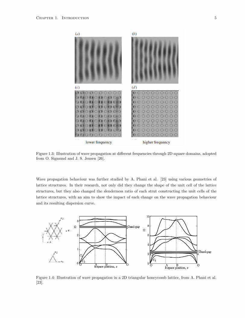
There has been extensive research on wave propagation through various 2D periodic lattices. O. Sig-
mund and J. S. Jensen illustrated two waves propagating at different frequencies in separate 2D square
domains, and reported the changes in wave propagation behaviours and the band gap phenomenon when
2D periodic circular inclusions were applied to each domain [26]. For example, Figure 1.3(a) illustrates
a wave propagating at low frequency in 2D square domain, while the Figure 1.3(b) shows another wave
propagating at a high frequency in a separate 2D square domain. When circular periodic inclusions
are introduced to each square domain, changes in wave propagation behaviour occur, as is presented in
the following figures. As illustrated in Figure 1.3(c), for a wave propagating at a lower frequency, wave
propagation is still present, but is distorted due to reflections and refraction from the periodic inclusions.
However, as illustrated in Figure 1.3(d), for a wave propagating at higher frequency, there is no wave
propagation, thus showing the band gap phenomenon.
Chapter 1. Introduction 5
Figure 1.3: Illustration of wave propagation at different frequencies through 2D square domains, adoptedfrom O. Sigmund and J. S. Jensen [26].
Wave propagation behaviour was further studied by A. Phani et al. [23] using various geometries of
lattice structures. In their research, not only did they change the shape of the unit cell of the lattice
structures, but they also changed the slenderness ratio of each strut constructing the unit cells of the
lattice structures, with an aim to show the impact of each change on the wave propagation behaviour
and its resulting dispersion curve.
Figure 1.4: Illustration of wave propagation in a 2D triangular honeycomb lattice, from A. Phani et al.[23].

Chapter 1. Introduction 6
In Figure 1.4, the left figure illustrates a triangular honeycomb lattice structure and its unit cell, while
the middle figure illustrates the dispersion curve obtained when the radius to length ratio is 0.1, and the
right figure illustrates the dispersion curve obtained when the radius to length ratio is 0.02. As can be
easily noted, the overall dispersion curve as well as band gap location is changed as the radius to length
ratio of the strut is changed from 0.1 to 0.02.
Figure 1.5: Illustration of wave propagation in a 2D square honeycomb lattice, from A. Phani et al. [23].
In Figure 1.5, the left figure illustrates a square honeycomb lattice structure and its unit cell, while the
middle figure depicts the dispersion curve obtained when the radius to length ratio is 0.1 and the right
figure shows the dispersion curve obtained when the radius to length ratio is 0.02. Compared to the
two dispersion curves obtained from triangular honeycomb lattices, the dispersion curves obtained from
square honeycomb lattices show entirely different dispersion curves, with no sign of a band gap for both
radius to length ratios.
1.4 Project Scope
There already exist a numerical model of wave propagation behaviour in 3D lattice structures developed
by Arya and Steeves [1]. This previous model is, therefore, used as a reference for this Master’s thesis.
The present thesis analyzes deeper on the relationships between the shape, design variables, and the
materials of the lattice structures and how these affect the resulting dispersion curves. Also, this thesis
provides a comparison of symmetric and non-symmetric lattice structures. A symmetric lattice is a
lattice structure where all the comprising struts share the same design variables and geometries; whereas
a non-symmetric lattice comprises one or more struts that have different design variables to the other
remaining struts. This study is aimed to discover whether having non-symmetric lattices, achieved
herein by introducing one or more modifications to the design variables, would allow a wider selection
of options when tailoring the lattice structures for the maximum band gap at a desired frequency range.
Chapter 1. Introduction 7
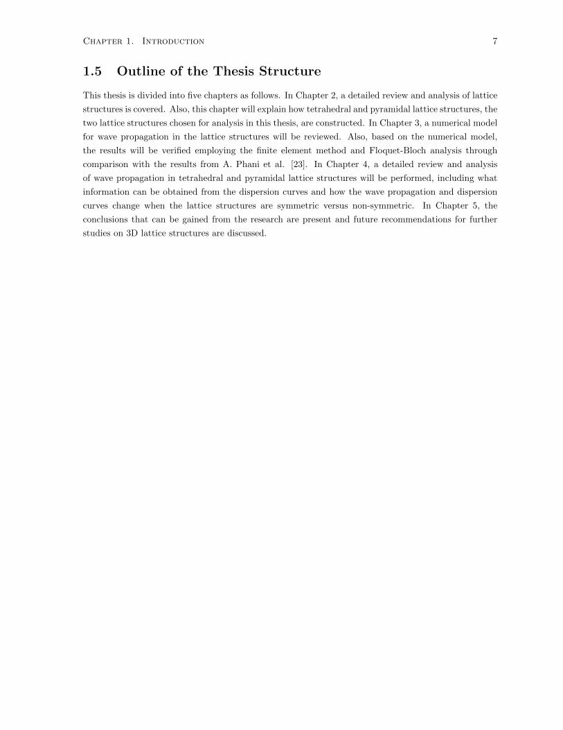
1.5 Outline of the Thesis Structure
This thesis is divided into five chapters as follows. In Chapter 2, a detailed review and analysis of lattice
structures is covered. Also, this chapter will explain how tetrahedral and pyramidal lattice structures, the
two lattice structures chosen for analysis in this thesis, are constructed. In Chapter 3, a numerical model
for wave propagation in the lattice structures will be reviewed. Also, based on the numerical model,
the results will be verified employing the finite element method and Floquet-Bloch analysis through
comparison with the results from A. Phani et al. [23]. In Chapter 4, a detailed review and analysis
of wave propagation in tetrahedral and pyramidal lattice structures will be performed, including what
information can be obtained from the dispersion curves and how the wave propagation and dispersion
curves change when the lattice structures are symmetric versus non-symmetric. In Chapter 5, the
conclusions that can be gained from the research are present and future recommendations for further
studies on 3D lattice structures are discussed.

Chapter 2
Periodic Lattice Structures
The main objective of this thesis is to construct 3D periodic lattice structures and then to analyze wave
propagation behaviours in the corresponding periodic lattice structures. In this paper, the analysis of the
wave propagations will be focused on tetrahedral and pyramidal 3D lattice structures. Also, a triangular
2D lattice structure is used to validate the numerical model for the analysis, through comparing the
results with those from the past research performed by A. Phani et al. [23].
In this chapter, background on the lattice structures will be reviewed, such as generating the physical
lattice structures and converting the physical lattices into the structure in wave-space, i.e. a reciprocal
lattice structure. Afterwards, the special properties of the periodic lattice structures and the advantages
of analyzing periodic lattice structures will be discussed.
2.1 Generating Physical Lattice Structures
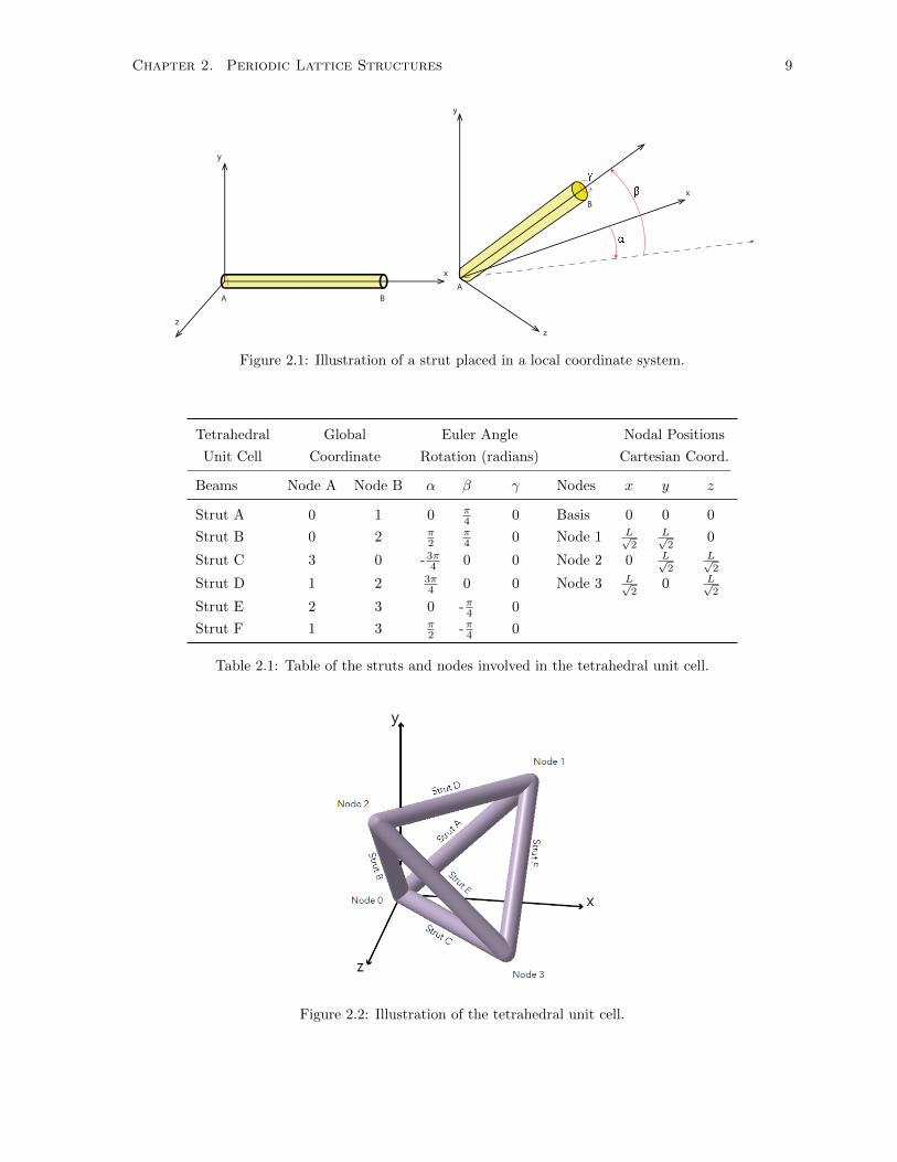
In order to construct a periodic lattice structure, a primitive unit cell must be defined. The unit cell
is constructed with multiple nodes and struts, arranged in specific angles to form a desired shape. The
struts are originally in a local coordinate system, placed horizontally along the abscissa (the x-axis).
Each of the struts in a local coordinate system are then transformed into a global coordinate system
through Euler angle rotations, α, β, and γ, where α is the angle rotated about the y-axis, β is the angle
rotated about the z-axis, and γ is the angle rotated about a struts central axis.
While the Euler angle rotations define the orientation of the struts of the lattice unit cell, nodes are
required to be assigned at each end of the struts to define the nodal connectivity. For instance, one
strut may have node A on the left end of the strut and node B on the right end, while another strut will
have node C on its left end and node A on its right end. When connecting these two struts, the struts
should be placed in such a way that the nodes of the same type, e.g. node A, from each strut should
coincide. Following the above design mechanism, 2D triangular unit lattice cell, and 3D tetrahedral and
pyramidal unit lattice cells can be generated.
8
Chapter 2. Periodic Lattice Structures 9
x
y
z
A B
A
B
z
x
y
Figure 2.1: Illustration of a strut placed in a local coordinate system.
Tetrahedral Global Euler Angle Nodal Positions
Unit Cell Coordinate Rotation (radians) Cartesian Coord.
Beams Node A Node B α β γ Nodes x y z
Strut A 0 1 0 π4 0 Basis 0 0 0
Strut B 0 2 π2
π4 0 Node 1 L√
2L√2
0
Strut C 3 0 - 3π4 0 0 Node 2 0 L√2
L√2
Strut D 1 2 3π4 0 0 Node 3 L√
20 L√
2
Strut E 2 3 0 -π4 0
Strut F 1 3 π2 -π4 0
Table 2.1: Table of the struts and nodes involved in the tetrahedral unit cell.
Figure 2.2: Illustration of the tetrahedral unit cell.

Chapter 2. Periodic Lattice Structures 10
Pyramidal Global Euler Angle Nodal Positions
Unit Cell Coordinate Rotation (radians) Cartesian Coord.
Beams Node A Node B α β γ Nodes x y z
Strut A 0 1 π2 0 0 Basis 0 0 0
Strut B 0 2 0 0 0 Node 1 0 0 L
Strut C 0 3 π4
π4 0 Node 2 L 0 0
Strut D 1 3 -π4π4 0 Node 3 L
2L√2
2L2
Strut E 4 3 - 3π4π4 0 Node 4 L 0 L
Strut F 2 3 3π4
π4 0
Table 2.2: Table of the struts and nodes involved in the pyramidal unit cell.
Node 1
Node 2
Node 3
Strut D
Strut A
Strut F
Stru
t E
Strut B
Str
ut
C
Node 0
Node 4
Figure 2.3: Illustration of the pyramidal unit cell.
The direct unit lattice contains n direct basis vectors, in which n is equal to the dimension of the lattice
structure. The 2D triangular unit lattice, therefore, has two basis vectors, and the 3D tetrahedral and
pyramidal unit lattice contains three basis vectors each. The direct basis vectors are defined such that
the entire lattice structure can be formed by tessellating the direct lattice along the basis vectors ei such
as e1, e2, and e3
Figure 2.4: Illustration of the tetrahedral lattice structure with the basis vectors.

Chapter 2. Periodic Lattice Structures 11
Figure 2.5: Illustration of the pyramidal lattice structure with the basis vectors.
2.2 Direct Lattice Structures in the Wave Space: Reciprocal
Lattices
The reciprocal lattice is a non-physical lattice consisting of reciprocal basis vectors, which are derived
from the direct lattice and its basis vectors. The reciprocal lattice is in k -space (momentum space),
which is the set of all wave vectors k, while the wave vectors are a frequency analog of the position
vector r. The reciprocal lattice is used through finite element analysis to obtain the wave propagation
behaviour in the lattice structure. The set of reciprocal basis vectors, e∗i , are defined by the following
equations:
For three-dimensional lattice structure: e∗1 = 2π (e2×e3)
e1·(e2×e3)
e∗2 = 2π (e3×e1)e1·(e2×e3)
e∗3 = 2π (e1×e2)e1·(e2×e3)
(2.1)
while ei = direct lattice basis vectors
e∗i = reciprocal lattice basis vectors
Following the governing relationship between direct basis vectors and reciprocal basis vectors, the re-
ciprocal basis vectors for 3D tetrahedral and pyramidal lattice structures are obtained. Each of the
tetrahedral and pyramidal lattice unit cells has three direct basis vectors and three reciprocal basis vec-
tors. In Figure 2.6, the three diagrams depict how each reciprocal basis vector of the tetrahedral unit
cell is defined based on the direct basis vectors of the unit cell. In the diagram, the red lines represent
the direct basis vectors of the tetrahedral unit cell, namely e1, e2, and e3, while the green lines represent
the reciprocal basis vectors of the same unit cell, namely e∗1, e∗2, and e∗3. The left diagram of Figure 2.6
illustrates how the reciprocal basis vector e∗1 is orthogonal to both the direct basis vectors e2 and e3,
while the middle diagram shows that the reciprocal basis vector e∗2 is orthogonal to both the direct basis
vectors e1 and e3, and the right diagram illustrates how the reciprocal basis vector e∗3 is orthogonal to
both the direct basis vectors e1 and e2, with all of the reciprocal basis vectors having an absolute value
of 2πunit cell length . The collection of the direct basis vectors of the tetrahedral unit cell is illustrated in
the left diagram of Figure 2.7, while the collection of the reciprocal basis vectors of the tetrahedral unit
cell is illustrated in the right diagram of Figure 2.7.

Chapter 2. Periodic Lattice Structures 12
Figure 2.6: Illustration of the relationship between the direct basis vectors and the reciprocal basisvectors.
Figure 2.7: Illustration of the direct basis vectors and reciprocal basis vectors of the tetrahedral unitcell.
Similarly, the governing relationship described above is applied to construct direct and reciprocal basis
vectors of the 3D pyramidal unit cell, which is illustrated in Figure 2.8. The left diagram of Figure 2.8
depicts the three direct basis vectors of the pyramidal unit cell, while the right diagram of Figure 2.8
depicts the three reciprocal basis vectors of the pyramidal unit cell.
Figure 2.8: Illustration of the direct basis vectors and reciprocal basis vectors of the pyramidal unit cell.
Chapter 2. Periodic Lattice Structures 13
2.3 Properties and Behaviour of Wave Propagation in an Infi-
nite Lattice Structure
2.3.1 Brillouin Zone in a Reciprocal Lattice
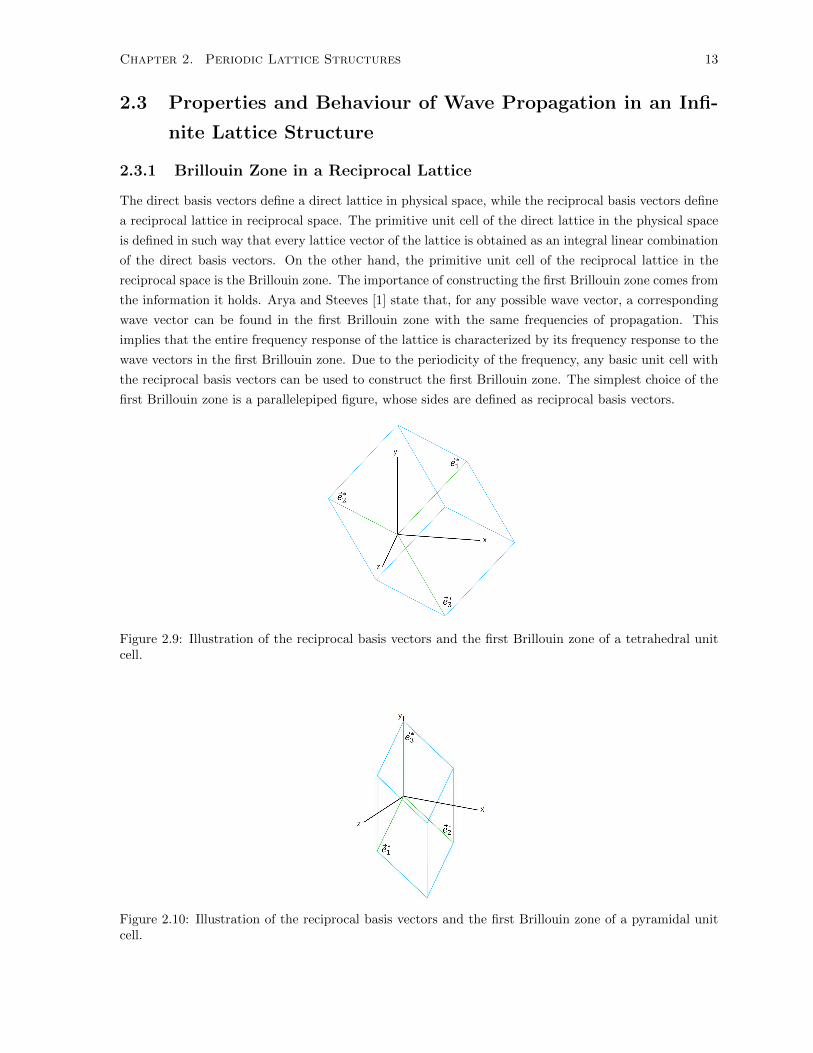
The direct basis vectors define a direct lattice in physical space, while the reciprocal basis vectors define
a reciprocal lattice in reciprocal space. The primitive unit cell of the direct lattice in the physical space
is defined in such way that every lattice vector of the lattice is obtained as an integral linear combination
of the direct basis vectors. On the other hand, the primitive unit cell of the reciprocal lattice in the
reciprocal space is the Brillouin zone. The importance of constructing the first Brillouin zone comes from
the information it holds. Arya and Steeves [1] state that, for any possible wave vector, a corresponding
wave vector can be found in the first Brillouin zone with the same frequencies of propagation. This
implies that the entire frequency response of the lattice is characterized by its frequency response to the
wave vectors in the first Brillouin zone. Due to the periodicity of the frequency, any basic unit cell with
the reciprocal basis vectors can be used to construct the first Brillouin zone. The simplest choice of the
first Brillouin zone is a parallelepiped figure, whose sides are defined as reciprocal basis vectors.
Figure 2.9: Illustration of the reciprocal basis vectors and the first Brillouin zone of a tetrahedral unitcell.
Figure 2.10: Illustration of the reciprocal basis vectors and the first Brillouin zone of a pyramidal unitcell.
Chapter 2. Periodic Lattice Structures 14
2.3.2 Floquet and Bloch Theorem
Floquet’s principal for one-dimensional (1D) lattice structures and Bloch’s theorem in higher dimensional
lattice structures are special cases of the wave equation in a periodic structure [23]. They are applied
to impose periodic boundary conditions and to turn problems in infinite lattice structures into finite
models, which enforce a plane wave solution in an infinite lattice. In 3D periodic structures with three
basis vectors, according to Bloch’s theorem, the classical equation to describe plane wave motion in the
3D periodic structure in terms of the relation between ~r (the position vector) and ~rj (the j th lattice
point in the reference cell) is stated below.
q(~r) = q(~rj)en1k1+n2k2+n3k3 (2.2)
while ~rj = lattice points in reference cell
~r = vector of lattice points in cell corresponding to
j th point in reference cell
q(~rj) = displacement of a lattice point in reference cell
ki = δi + iεi = Wave vectors of plane wave
δi = Attenuation constants along basis vector ei
εi = Phase constants
(n1, n2, n3) = integer tuple that defines specific cell in the lattice,
which the cell is located at n1 distance along e1 direction,
n2 distance along e2 direction, and n3 distance along e3 direction
in relation to the reference cell
The wave vectors of a plane wave, k, are complex, containing a real part and an imaginary part, where
the real part is the attenuation constant and the imaginary part is the phase constant [23]. Attenuation
describes the gradual loss of intensity of a planar wave through a lattice structure. For waves propagating
without attenuation in any lattice structure, the real part of the wave vector k is equal to zero, and the
change in amplitude of the complex wave across the lattice structure does not depend on the location
of the unit cell in the structure. Therefore, Bloch’s theorem implies that one can study and understand
wave propagation through the entire lattice structure by considering wave motion within a single unit
cell, saving a large amount of time in the analysis of wave propagation in a lattice structure.
2.3.3 Coated Polymer Lattice Structure: An Ultralight Structure
At the beginning of the thesis, it was mentioned that periodic lattice structures can contribute to
sustainable aviation as an application of ultralight materials. The following are two examples of periodic
lattice structures with a radius to length ratio of 1 to 10, specifically with the radius being 1 mm and the
length 10 mm. For the analysis of the wave propagation behaviour in 3D lattice structures throughout
this thesis, the structures are considered to be coated with a nanometal. The radius and the length as
well as the coating thickness of the struts are potential design variables, which can be modified to give
different resulting dispersion curves and band gap phenomena in each lattice structure. For the coated
prototype model shown below, the coating thickness for both samples was set at 25 microns. It should
be noted that there is a thin layer of copper beneath the nickel layer, with the reason for this being so
that there is a metal surface for the electrodeposition process of nickel. Otherwise, if the nickel layer

Chapter 2. Periodic Lattice Structures 15
were put directly onto the polymer instead, it would become an electroless process, which would not
produce as thick a coating as that from the electrodeposition process.
Figure 2.11: Illustration of the coated lattice structures.
The dimensions of the bounding box, the smallest rectangular prism box that envelops the lattice
structure, for each lattice structure were measured. The volume of the bounding box represents the
volume of the solid plate. Based on the volume of the bounding box and the volume of the lattice
structure for each model, the relative density, which defines the volume fraction of the space filled with
material as a percentage of the total volume of the lattice was measured. The tetrahedral lattice structure
had 20.19% of material of relative density, while the pyramidal lattice structure had 20.62% of material
of relative density.
relative density =volume of the lattice structure
volume of the solid plate (of the same bounding box dimensions)(2.3)
Lattice Geometry
Properties Tetrahedral Lattice Pyramidal Lattice
Bounding Box 6.2 × 5.97 × 5.098 cm 6.2 × 6.2 × 4.44 cm
Volume of Bounding Box 188.6974 cm3 170.6736 cm3
Volume of Lattice Struc. 38.098 cm3 35.1929 cm3
Relative Density 20.19 % 20.62 %
Table 2.3: Table of the relative densities of tetrahedral and pyramidal lattice structures.

Chapter 3
Finite Element Analysis
In this chapter, finite element analysis on the wave propagation behaviour through a 3D lattice structure
is discussed. The periodic lattice structures created from Chapter 2 will be used as the basic structure for
the numerical analysis. This chapter will discuss various design variables of the coated lattice structures,
and will then construct an eigenvalue problem through finite element analysis. By selecting the desired
wave numbers, the eigenvalue problem will be solved to find eigenfrequencies and mode shapes of the
wave propagating through the corresponding lattice structures.
3.1 Defining the Input Parameters
The coated lattice structure, constructed in the previous chapter, for the analysis of wave propagation
contains five design variables: length of each strut of the lattice structure (L), radius of the polymer struts
(rp), thickness of copper coating layer (tcu), thickness of nickel coating layer (tni), Young’s modulus and
the density of the polymer strut (Ep and ρp) and of each layer of coating. First, based on the Young’s
modulus and the radius of the polymer substrate, as well as the Young’s modulus and the thickness
of the copper (Ecu and ρcu) and nickel (Eni and ρni) coating layers, the flexural rigidity of the overall
coated structure (Ecs) was calculated.
EcsIcs = EpIp + EcuIcu + EniIni (3.1)
In the above equation, E is the Young’s modulus and I is the second moment of area of each section of
the strut. The second moment of area for the solid polymer strut (cylindrical shape) is defined as Icy
and the second moment of area for the coating layers (hollowed cylindrical shape, annulus) is defined as
Ian, which are expressed as
Icy =πr4
4(3.2)
Ian =π(r4or − r4ir)
4(3.3)
For the prototype tetrahedral and pyramidal lattice structures, the input parameters were set as follows.
16
Chapter 3. Finite Element Analysis 17
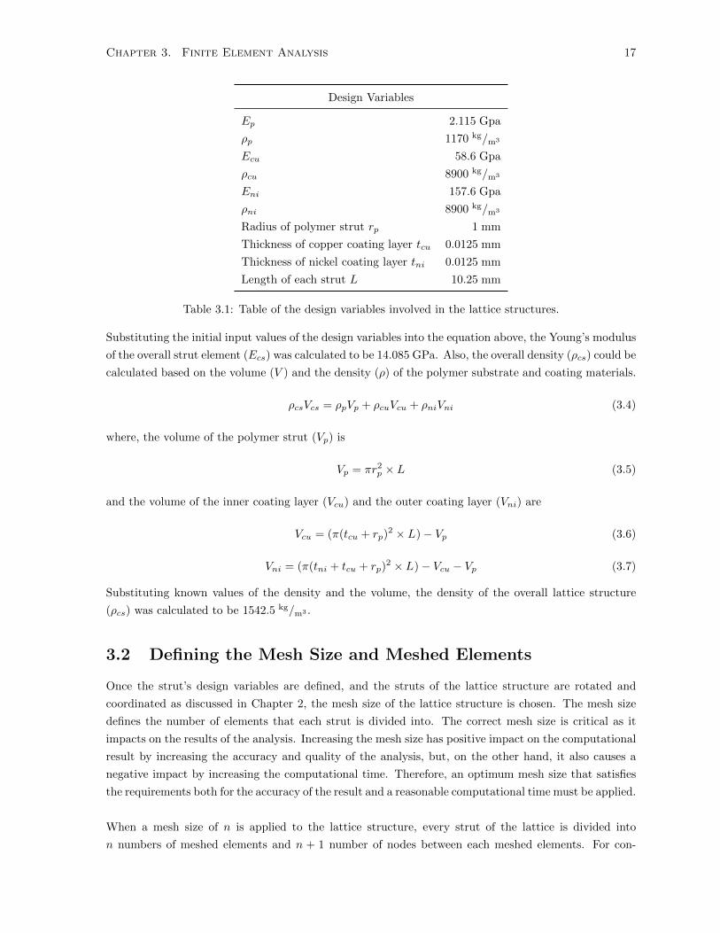
Design Variables
Ep 2.115 Gpa
ρp 1170 kg/m3
Ecu 58.6 Gpa
ρcu 8900 kg/m3
Eni 157.6 Gpa
ρni 8900 kg/m3
Radius of polymer strut rp 1 mm
Thickness of copper coating layer tcu 0.0125 mm
Thickness of nickel coating layer tni 0.0125 mm
Length of each strut L 10.25 mm
Table 3.1: Table of the design variables involved in the lattice structures.
Substituting the initial input values of the design variables into the equation above, the Young’s modulus
of the overall strut element (Ecs) was calculated to be 14.085 GPa. Also, the overall density (ρcs) could be
calculated based on the volume (V ) and the density (ρ) of the polymer substrate and coating materials.
ρcsVcs = ρpVp + ρcuVcu + ρniVni (3.4)
where, the volume of the polymer strut (Vp) is
Vp = πr2p × L (3.5)
and the volume of the inner coating layer (Vcu) and the outer coating layer (Vni) are
Vcu = (π(tcu + rp)2 × L)− Vp (3.6)
Vni = (π(tni + tcu + rp)2 × L)− Vcu − Vp (3.7)
Substituting known values of the density and the volume, the density of the overall lattice structure
(ρcs) was calculated to be 1542.5 kg/m3 .
3.2 Defining the Mesh Size and Meshed Elements
Once the strut’s design variables are defined, and the struts of the lattice structure are rotated and
coordinated as discussed in Chapter 2, the mesh size of the lattice structure is chosen. The mesh size
defines the number of elements that each strut is divided into. The correct mesh size is critical as it
impacts on the results of the analysis. Increasing the mesh size has positive impact on the computational
result by increasing the accuracy and quality of the analysis, but, on the other hand, it also causes a
negative impact by increasing the computational time. Therefore, an optimum mesh size that satisfies
the requirements both for the accuracy of the result and a reasonable computational time must be applied.
When a mesh size of n is applied to the lattice structure, every strut of the lattice is divided into
n numbers of meshed elements and n + 1 number of nodes between each meshed elements. For con-

Chapter 3. Finite Element Analysis 18
vention, original struts prior to meshing are referred as the parent struts, while the meshed elements of
the corresponding struts are referred to as child elements. As discussed in the previous chapter, parent
struts contain Euler rotation angles, and a positive node and negative node at each end. Negative nodes
refer to nodes at x = 0, while positive nodes refer to nodes at x = L, when the parent strut is placed
in local coordinate system. When meshed elements are created, each child element inherits the same
Euler rotation angle from its corresponding parent struts as well as the direction where the positive and
negative nodes are located. The nodes at each end of the child elements are shared and bounded by the
adjacent child elements.
Figure 3.1: Illustration of the negative and positive nodes of the parent struts and meshed elements.
3.3 Defining the Nodes of the Structure
For an infinite lattice structure, Bloch’s theorem relates the displacements at certain nodes in the unit
cell to the displacements at the basis node [1]. Therefore, once the unit lattice structure is constructed,
and the structure is meshed into the desired number of elements, the nodes must be defined into different
categories: basis, internal, and boundary. Typically, a node located at the origin of the coordinate system
is defined as the basis node, qb, and is used as a base reference node to describe the boundary nodes. The

Chapter 3. Finite Element Analysis 19
boundary nodes, qbnd, are the nodes that can be reached by traversing the basis node along the direction
of the direct basis vectors e1, e2, e3. The boundary nodes are shared by other neighbouring unit cells
in the lattice structures. Therefore, typically the nodes at the end of each parent strut in the direction
of the direct basis vectors are defined as the boundary nodes. Lastly, nodes created between each of the
meshed element are defined as internal nodes, qi, which are not shared by the other neighbouring unit
cells.
Tetrahedral Negative Node Positive Node
Strut A Basis Boundary e1
Strut B Basis Boundary e2
Strut C Boundary e3 Basis
Strut D Boundary e1 Boundary e2
Strut E Boundary e2 Boundary e3
Strut F Boundary e1 Boundary e3
Table 3.2: Table of the internal, basis, and boundary nodes involved in the tetrahedral unit cell.
Boundary Node
Strut D
Strut A
Stru
t F
Strut E
Stru
t B
Strut C
Boundary Node
Boundary Node
Basis Node
Figure 3.2: Illustration of the tetrahedral unit cell with the negative and the positive nodes of each strutdefined in Table 3.2.
Pyramidal Negative Node Positive Node
Strut A Basis Boundary e1
Strut B Boundary e2 Basis
Strut C Basis Boundary e3
Strut D Boundary e1 Boundary e3
Strut E Boundary e12 Boundary e3
Strut F Boundary e2 Boundary e3
Table 3.3: Table of the internal, basis, and boundary nodes involved in the pyramidal unit cell.

Chapter 3. Finite Element Analysis 20
Figure 3.3: Illustration of the pyramidal unit cell with the negative and the positive nodes of each strutdefined in Table 3.3.
3.4 Defining Direct Basis Vectors and Reciprocal Basis Vectors
After all the meshed elements and nodes are defined, three direct basis vectors, namely e1, e2, and e3
are constructed, which are based on Cartesian coordinates as follows.
[e1 e2 e3
]=
e1x e2x e3x
e1y e2y e3y
e1z e2z e3z
(3.8)
Based on the direct basis vectors, ei, in the Cartesian form described above, the reciprocal basis vectors,
e∗i, can be obtained. While the geometrical relationship between the direct basis vectors and reciprocal
basis vectors are defined in Chapter 2, the numerical relationship between the direct and the reciprocal
basis vectors can be expressed as follows.
2π[e1 e2 e3
]−1=[e∗1 e∗2 e∗3
]T(3.9)
Therefore, it can be seen that the reciprocal basis vectors are the inverse transpose of the direct basis
vectors. [2π[ e1 e2 e3 ]−1
]T=[e∗1 e∗2 e∗3
](3.10)

Chapter 3. Finite Element Analysis 21
3.5 Defining the Brillouin Zone
The Brillouin zone is defined by constructing a parallelepiped figure based on the reciprocal basis vectors.
The Brillouin zone is turned into a 3D grid system (e∗1, e∗2, e∗3), where each coordinate of the grid
represents a wave vector, k = (k1, k2, k3). The grid size of the Brillouin zone affects the total number
of wave vectors that can be obtained from the Brillouin zone. When the Brillouin zone is turned into
an n×n×n grid system, there are a total of (n+ 3)3 numbers of wave vectors. The increase in the grid
size gives a greater number of (finer) wave vectors to analyze, thus increasing the accuracy and quality
of the results.
3.6 Defining Eigenvalue Problems
3.6.1 Timoshenko Beams and Nodal Displacements
The constructed lattice structures and meshed elements are considered as Timoshenko beams. Timo-
shenko beams are preferred and selected over Euler-Bernoulli beams, as the dispersion relation of the
Euler-Bernoulli beam theory predicts that waves of short wavelength travel with unlimited speed, which
is unrealistic. This unrealistic prediction arises due to two assumptions of the Euler-Bernoulli beam
theory, namely that rotational effects are neglected and that the beam element remains rectangular
during motion. However, in reality, waves of short wavelength will cause rotation and deformation of the
beam element, hence leading to unrealistic predictions on the dispersion relation for short wavelengths.
Contrary to Euler-Bernoulli beam theory, the Timoshenko beam theory takes account of the rotation
and shear deformation of the beam element for waves of short wavelength, thus making it suitable for
describing the dispersion relations of lattice structures.
Each 3D Timoshenko element has two nodes with six displacements for each node: υ, ν, ω, φ, ψ,
θ. The υ, ν, and ω are the translational displacements along the x-axis, y-axis, and z-axis, in corre-
sponding order, and the other three, φ, ψ, and θ, are rotational displacements about the x-axis, y-axis,
and z-axis in corresponding order. Hence, the displacement of a single element qel with node A and node
B can be described as[qel
]=[qA qB
]T=[υA νA ωA φA ψA θA υB νB ωB φB ψB θB
]T(3.11)
Therefore, displacements in a single strut qst meshed into three elements, with its containing nodes
categorized into different types as discussed in the previous section, can be described as
[qst
]=[qi1 qi2 qb qbnd
]T(3.12)

Chapter 3. Finite Element Analysis 22
x
y
z
A B
Figure 3.4: Illustration of the nodal displacements involved in each 3D strut.
3.7 Setting up the Shape Functions
According to the standard finite element procedure, the elastic deformation of an arbitrary point x of
the 3D two-node meshed element, at time t can be expressed as [3][d]
=[N]
.[qel
](3.13)
where [d] represents the elastic deformation vector of the meshed element, [N ] represents the matrix of
shape functions, and qel represents the nodal displacement vector.
υ(x, t) = ai(x)qel(t) (3.14a)
ν(x, t) = bi(x)qel(t) (3.14b)
ω(x, t) = ci(x)qel(t) (3.14c)
φ(x, t) = di(x)qel(t) (3.14d)
ψ(x, t) = ei(x)qel(t) (3.14e)
θ(x, t) = fi(x)qel(t) (3.14f)
where, [qel
]=[υA νA ωA φA ψA θA υB νB ωB φB ψB θB
]T(3.15)
ai
bi
ci
di
ei
fi
T
=
a1 a2 a3 a4 a5 a6 a7 a8 a9 a10 a11 a12
b1 b2 b3 b4 b5 b6 b7 b8 b9 b10 b11 b12
c1 c2 c3 c4 c5 c6 c7 c8 c9 c10 c11 c12
d1 d2 d3 d4 d5 d6 d7 d8 d9 d10 d11 d12
e1 e2 e3 e4 e5 e6 e7 e8 e9 e10 e11 e12
f1 f2 f3 f4 f5 f6 f7 f8 f9 f10 f11 f12
T
(3.16)

Chapter 3. Finite Element Analysis 23
ai
bi
ci
di
ei
fi
T
=
a1 0 0 0 0 0 a7 0 0 0 0 0
0 b2 0 0 0 b6 0 b8 0 0 0 b12
0 0 c3 0 c5 0 0 0 c9 0 c11 0
0 0 0 d4 0 0 0 0 0 d10 0 0
0 0 e3 0 e5 0 0 0 e9 0 e11 0
0 f2 0 0 0 f6 0 f8 0 0 0 f12
T
(3.17)
The shape functions of a 3D Timoshenko beam element are defined as follows [1, 3]:
a1 = 1− ξ (3.18a)
a7 = ξ (3.18b)
b2 = µz[1− 3ξ2 + 2ξ3 + ηz(1− ξ)
](3.18c)
b6 = Lµz
[ξ − 2ξ2 + ξ3 +
ηz2
(ξ − ξ2)]
(3.18d)
b8 = µz[3ξ2 − 2ξ3 + ηzξ
](3.18e)
b12 = Lµz
[−ξ2 + ξ3 +
ηz2
(−ξ + ξ2)]
(3.18f)
c3 = µy[1− 3ξ2 + 2ξ3 + ηy(1− ξ)
](3.18g)
c5 = −Lµy[ξ − 2ξ2 + ξ3 +
ηy2
(ξ − ξ2)]
(3.18h)
c9 = µy[3ξ2 − 2ξ3 + ηyξ
](3.18i)
c11 = −Lµy[−ξ2 + ξ3 +
ηy2
(−ξ + ξ2)]
(3.18j)
d4 = 1− ξ (3.18k)
d10 = ξ (3.18l)
e3 = −6µyL
[−ξ + ξ2
](3.18m)
e5 = µy[1− 4ξ + 3ξ2 + ηy(1− ξ)
](3.18n)
e9 = −6µyL
[ξ − ξ2
](3.18o)
e11 = µz[−2ξ + 3ξ2 + ηyξ
](3.18p)
f2 =6µzL
[−ξ + ξ2
](3.18q)
f6 = µz[1− 4ξ + 3ξ2 + ηz(1− ξ)
](3.18r)
f8 =6µzL
[ξ − ξ2
](3.18s)
f12 = µz[−2ξ + 3ξ2 + ηzξ
](3.18t)

Chapter 3. Finite Element Analysis 24
ξ =x
L(3.19a)
ηy =12EIyκGAL2
(3.19b)
ηz =12EIzκGAL2
(3.19c)
µy =1
1 + ηy(3.19d)
µz =1
1 + ηz(3.19e)
κ = Shear correction factor =6(1 + ν)
7 + 6ν(3.19f)
ν = Poisson’s ratio (3.19g)
E = Young’s modulus (3.19h)
Iy,z = Second moment of area (3.19i)
A = Cross section of the strut element (3.19j)
L = Length of the strut element (3.19k)
3.8 Kinetic Energy of a Timoshenko Beam: Setting the Local
Mass Matrix
First, the kinetic energy of a Timoshenko element is expressed in terms of the nodal displacements, while
the kinetic energy of a particle i is described as
Ti =1
2mivi
2 (3.20)
and the total kinetic energy of the system becomes the sum of the kinetic energies of all particles in the
system:
Tsys =
n∑i=1
Ti =
n∑i=1
1
2mivi
2 (3.21)
For a rigid body, such as a Timoshenko beam element, the equation becomes
Tel =
∫m
1
2|~v|2 dm (3.22)
To continue derivation of the kinetic energy equation of the Timoshenko element, the expression for the
displacement field must be obtained. Figure 3.5 illustrates the motion of a particle p at an arbitrary
location in 3D beam, and the location of the particle after displacement, p′.

Chapter 3. Finite Element Analysis 25
Figure 3.5: Illustration of the kinematics of a particle in a 3D strut [16].
Vector r, which describes the location of particle p, can be divided into two components: rc and t, where
rc is the vector defining the location of the point c, which is point p projected onto the central axis
(x-axis) and t is the vector from point c, directed to point p.
[r]
=
x
y
z
(3.23)
[rc
]=
x
0
0
(3.24)
[t]
=
0
y
z
(3.25)
r = rc + t (3.26)
t = r − rc (3.27)
Likewise, the vector r′ describing the location of the particle after the displacement, is expressed as
r′ = r′c + t′ (3.28)
Based on Euler-Chasles’ theorem, the rotation of vector t can be described by the rotational matrix R
[16]:
t′ = Rt (3.29)
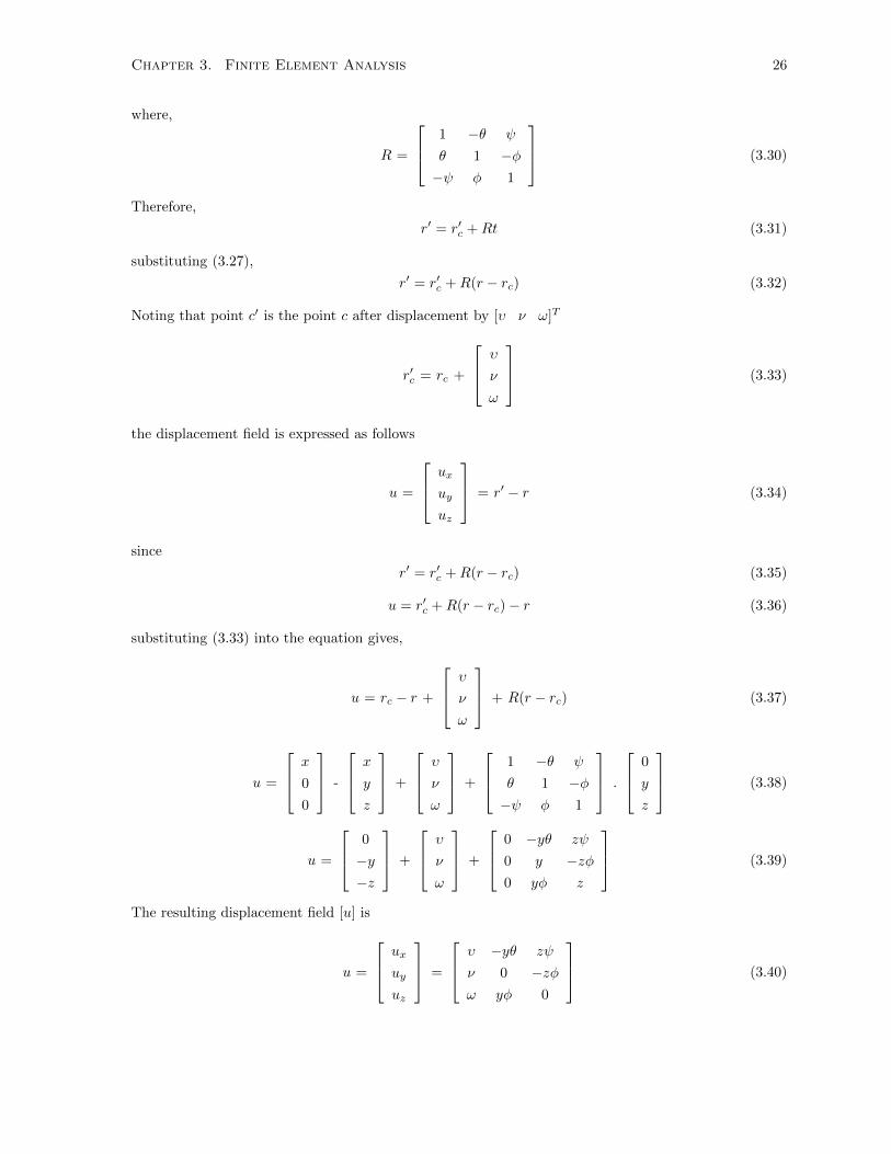
Chapter 3. Finite Element Analysis 26
where,
R =
1 −θ ψ
θ 1 −φ−ψ φ 1
(3.30)
Therefore,
r′ = r′c +Rt (3.31)
substituting (3.27),
r′ = r′c +R(r − rc) (3.32)
Noting that point c′ is the point c after displacement by [υ ν ω]T
r′c = rc +
υ
ν
ω
(3.33)
the displacement field is expressed as follows
u =
ux
uy
uz
= r′ − r (3.34)
since
r′ = r′c +R(r − rc) (3.35)
u = r′c +R(r − rc)− r (3.36)
substituting (3.33) into the equation gives,
u = rc − r +
υ
ν
ω
+ R(r − rc) (3.37)
u =
x
0
0
-
x
y
z
+
υ
ν
ω
+
1 −θ ψ
θ 1 −φ−ψ φ 1
.
0
y
z
(3.38)
u =
0
−y−z
+
υ
ν
ω
+
0 −yθ zψ
0 y −zφ0 yφ z
(3.39)
The resulting displacement field [u] is
u =
ux
uy
uz
=
υ −yθ zψ
ν 0 −zφω yφ 0
(3.40)
Chapter 3. Finite Element Analysis 27
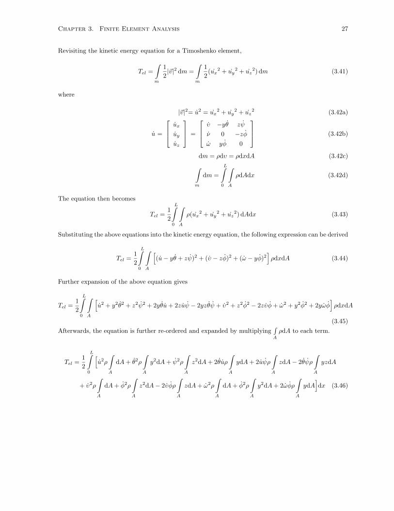
Revisiting the kinetic energy equation for a Timoshenko element,
Tel =
∫m
1
2|~v|2 dm =
∫m
1
2(ux
2 + uy2 + uz
2) dm (3.41)
where
|~v|2= u2 = ux2 + uy
2 + uz2 (3.42a)
u =
ux
uy
uz
=
υ −yθ zψ
ν 0 −zφω yφ 0
(3.42b)
dm = ρdυ = ρdxdA (3.42c)∫m
dm =
L∫0
∫A
ρdAdx (3.42d)
The equation then becomes
Tel =1
2
L∫0
∫A
ρ(ux2 + uy
2 + uz2) dAdx (3.43)
Substituting the above equations into the kinetic energy equation, the following expression can be derived
Tel =1
2
L∫0
∫A
[(u− yθ + zψ)2 + (υ − zφ)2 + (ω − yφ)2
]ρdxdA (3.44)
Further expansion of the above equation gives
Tel =1
2
L∫0
∫A
[u2 + y2θ2 + z2ψ2 + 2yθu+ 2zuψ − 2yzθψ + υ2 + z2φ2 − 2zυφ+ ω2 + y2φ2 + 2yωφ
]ρdxdA
(3.45)
Afterwards, the equation is further re-ordered and expanded by multiplying∫A
ρdA to each term.
Tel =1
2
L∫0
[u2ρ
∫A
dA+ θ2ρ
∫A
y2dA+ ψ2ρ
∫A
z2dA+ 2θuρ
∫A
ydA+ 2uψρ
∫A
zdA− 2θψρ
∫A
yzdA
+ υ2ρ
∫A
dA+ φ2ρ
∫A
z2dA− 2υφρ
∫A
zdA+ ω2ρ
∫A
dA+ φ2ρ
∫A
y2dA+ 2ωφρ
∫A
ydA]dx (3.46)
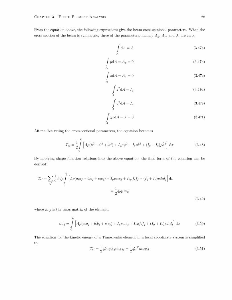
Chapter 3. Finite Element Analysis 28
From the equation above, the following expressions give the beam cross-sectional parameters. When the
cross section of the beam is symmetric, three of the parameters, namely Ay, Az, and J , are zero.
∫A
dA = A (3.47a)
∫A
ydA = Ay = 0 (3.47b)
∫A
zdA = Az = 0 (3.47c)
∫A
z2dA = Iy (3.47d)
∫A
y2dA = Iz (3.47e)
∫A
yzdA = J = 0 (3.47f)
After substituting the cross-sectional parameters, the equation becomes
Tel =1
2
L∫0
[Aρ(u2 + υ2 + ω2) + Iyρψ
2 + Izρθ2 + (Iy + Iz)ρφ
2]
dx (3.48)
By applying shape function relations into the above equation, the final form of the equation can be
derived:
Tel =∑ij
1
2qiqj
L∫0
[Aρ(aiaj + bibj + cicj) + Iyρeiej + Izρfifj + (Iy + Iz)ρdidj
]dx
=1
2qiqjmij
(3.49)
where mij is the mass matrix of the element.
mij =
L∫0
[Aρ(aiaj + bibj + cicj) + Iyρeiej + Izρfifj + (Iy + Iz)ρdidj
]dx (3.50)
The equation for the kinetic energy of a Timoshenko element in a local coordinate system is simplified
to
Tel =1
2˙qel i ˙qel jmel ij =
1
2˙qelTmel ˙qel (3.51)

Chapter 3. Finite Element Analysis 29
3.9 Strain Potential Energy of a Timoshenko Beam: Setting
the Local Stiffness Matrix
After the kinetic energy relation and the mass matrix of the Timoshenko element are found, the strain
potential energy of the Timoshenko element is calculated.
Uel =
∫V
U dV (3.52)
where U is the expression for the strain energy density:
U =
εij∫0
σijdεij (3.53)
For the strain energy density of isotropic materials, Hooke’s Law states that
σij = Cijklεkl = λεkkδij + 2Gεij (3.54)
where λ is Lame’s first parameter and G is Lame’s second parameter. The strain energy density equation
then becomes
U =
εij∫0
Cijklεkldεij =1
2Cijklεklεij (3.55)
Substituting the strain energy density equation and Hooke’s law for an isotropic material, the strain
potential energy equation for a Timoshenko element can be expressed as
Uel =
∫V
1
2CijklεklεijdV =
1
2
∫V
(λεkkδij + 2Gεij)εij dV (3.56)
Expanding and re-ordering,
Uel =1
2
∫V
(λεijεkkδij + 2Gεijεij) dV (3.57)
where,
εijεkkδij =
[3∑k=1
εkk
]2(3.58)
and
εijεij =
3∑i=1
3∑j=1
(ε2ij) (3.59)
[ε] =
ε11 ε12 ε13
ε21 ε22 ε23
ε31 ε32 ε33
(3.60)

Chapter 3. Finite Element Analysis 30
Revisiting the displacement field obtained above, the 3D stress-strain relations components can be
expressed as follows, where ux, uy, uz are the components of the displacement field.
ε11 =∂ux∂x
= u′ − yθ′ + zψ′ (3.61a)
ε22 =∂uy∂y
= 0 (3.61b)
ε33 =∂uz∂z
= 0 (3.61c)
ε12 = ε21 =1
2
(∂ux∂y
+∂uy∂x
)=
1
2(υ′ − zφ′ − θ) (3.61d)
ε13 = ε31 =1
2
(∂ux∂z
+∂uz∂x
)=
1
2(ω′ + yφ′ + ψ) (3.61e)
ε23 = ε32 =1
2
(∂uy∂z
+∂uz∂y
)= 0 (3.61f)
Therefore, the strain potential energy equation becomes,
Uel =1
2
∫V
[λ(ε11)2 + 2G(ε211 + 2ε212 + 2ε213)
]dV
=1
2
∫V
[λ(ε211) + 2G(ε211) + 4G(ε212) + 4G(ε213)
]dV
=1
2
∫V
[(λ+ 2G)(ε211) + 4G(ε212) + 4G(ε213)
]dV (3.62)
Substituting the strain expressions above,
Uel =1
2
∫V
[(λ+ 2G)
[(u′ − yθ′ + zψ′)2
]+ 4G
[(1
2(υ′ − zφ′ − θ)
)2]+ 4G
[(1
2(ω′ + yφ′ + ψ)
)2]]dV
=1
2
∫V
[(λ+ 2G)
[(u′ − yθ′ + zψ′)2
]+G (υ′ − zφ′ − θ)2 +G (ω′ + yφ′ + ψ)
2]
dV (3.63)
Replacing, ∫V
dV =
L∫0
∫A
dAdx (3.64)
the equation becomes
Uel =1
2
L∫0
∫A
[(λ+ 2G)
[(u′ − yθ′ + zψ′)2
]+G (υ′ − zφ′ − θ)2 +G (ω′ + yφ′ + ψ)
2]
dAdx (3.65)

Chapter 3. Finite Element Analysis 31
Expanding,
Uel =1
2
L∫0
∫A
[(λ+ 2G)(u′2 − 2yu′θ′ + 2zu′ψ′ − 2yzθ′ψ′ + y2θ′2 + z2ψ′2)
+G(υ′2 − 2zυ′φ′ − 2υ′θ + 2zφ′θ + z2φ′2 + θ2)
+G(ω′2 + 2yω′φ′ + 2ω′ψ + 2yφ′ψ + y2φ′2 + ψ2)]dAdx (3.66)
Afterwards, the equation can be further re-ordered and expanded by multiplying∫A
dA to each term
Uel =1
2
L∫0
[(λ+2G
)(u′2∫A
dA−2u′θ′∫A
ydA+2u′ψ′∫A
zdA−2θ′ψ′∫A
yzdA+θ′2∫A
y2dA+ψ′2∫A
z2dA)
+G(υ′2∫A
dA− 2υ′φ′∫A
zdA− 2υ′θ
∫A
dA+ 2φ′θ
∫A
zdA+ φ′2∫A
z2dA+ θ2∫A
dA)
+G(ω′2∫A
dA+ 2ω′φ′∫A
ydA+ 2ω′ψ
∫A
dA+ 2φ′ψ
∫A
ydA+ φ′2∫A
y2dA+ ψ2
∫A
dA)]
dx (3.67)
Afterwards, the expressions for the symmetric beam cross-sectional parameters are substituted into the
equation above to simplify the expression. ∫A
dA = A (3.68a)
∫A
ydA = Ay = 0 (3.68b)
∫A
zdA = Az = 0 (3.68c)
∫A
z2dA = Iy (3.68d)
∫A
y2dA = Iz (3.68e)
∫A
yzdA = J = 0 (3.68f)
A reduced form of the equation can be found:
Uel =1
2
L∫0
[λ(Au′2 + Iyψ
′2 + Izθ′2) + 2G(Au′2 + Iyψ
′2 + Izθ′2)
+G(Aυ′2 − 2Aυ′θ +Aθ2 + Iyφ′2) +G(Aω′2 + 2Aω′ψ + Izφ
′2 +Aψ2)]dx (3.69)

Chapter 3. Finite Element Analysis 32
Expanding the above equation and re-ordering,
Uel =1
2
L∫0
[λ(Au′2 + Iyψ
′2 + Izθ′2) + 2G(Au′2 + Iyψ
′2 + Izθ′2)
+GA(υ′2 − 2υ′θ + θ2) +GA(ω′2 + 2ω′ψ + ψ2) +G(Iyφ′2 + Izφ
′2)]dx
=1
2
L∫0
[λ(Au′2+Iyψ
′2+Izθ′2)+2G(Au′2+Iyψ
′2+Izθ′2)+GA
((υ′−θ)2+(ω′+ψ)2
)+G(Iy+Iz)φ
′2]dx
(3.70)
By substituting the expressions for the shape functions into the above derivative terms, and incorporating
the shear correction factor κ, the following form is derived.
Uel =1
2
L∫0
[λ(A(qia
′i)
2 + Iy(qie′i)
2 + Iz(qif′i)
2)
+ 2κG(A(qia
′i)
2 + Iy(qie′i)
2 + Iz(qif′i)
2)
+ κGA(
(qib′i − qifi)2 + (qic
′i + qiei)
2)
+ κG(Iy + Iz)(qid′i)
2]dx (3.71)
Uel =∑ij
1
2qiqj
L∫0
[λ(Aa′ia
′j + Iye
′ie′j + Izf
′if′j) + 2κG(Aa′ia
′j + Iye
′ie′j + Izf
′if′j)
+ κGA(
(b′i − fi)(b′j − fj) + (c′i + ei)(c′j + ej)
)+ κG(Iz + Iy)(d′id
′j)]dx
=1
2qiqjkij (3.72)
where, kij is the mass matrix of the element.
kij =
L∫0
[λ(Aa′ia
′j + Iye
′ie′j + Izf
′if′j) + 2κG(Aa′ia
′j + Iye
′ie′j + Izf
′if′j)
+ κGA(
(b′i − fi)(b′j − fj) + (c′i + ei)(c′j + ej)
)+ κG(Iz + Iy)(d′id
′j)]dx (3.73)
The equation for the strain potential energy of a Timoshenko element in a local coordinate system can
be simplified to
Uel =1
2qel iqel jkel ij =
1
2qTelkelqel (3.74)
where λ and G are the first and the second Lame’s parameters of the coated struts of the lattice
structures. First, Lame’s second parameter, G (shear modulus), is evaluated by the following, knowing
that the shear modulus, G, can be related with shear stress and shear strain:

Chapter 3. Finite Element Analysis 33
G =Shear Stress
Shear Strain=τxyγxy
=F/A
4x/l=
Fl
A4x(3.75)
where,
F = Shear force
A = Area of cross section
l = Length of the strut element
4x = Transverse displacement
re-ordering the equation, and equating to Shear Force,
F =GA4x
l(3.77)
GA4xl cs
=GA4x
l p+GA4x
l cu+GA4x
l ni(3.78)
Knowing that all the components of the coated strut have the same strut length and transverse displace-
ment, 4x and l can be eliminated from all the terms, resulting in the following equation
GAcs = GAp +GAcu +GAni (3.79)
Once Gcs is calculated, Lame’s first parameter can be found by using the following equation.
λ =G(E − 2G)
3G− E(3.80)
where E is the Young’s modulus of the overall coated strut found at the beginning of this chapter.
3.10 Evaluating the Shape Functions Involved in the Mass and
Stiffness Matrices
In the previous section, expressions for the local element mass and stiffness matrices, mij and kij , were
found based on the kinetic and strain potential energy equations.
mij =
L∫0
[Aρ(aiaj + bibj + cicj) + Iyρeiej + Izρfifj + (Iy + Iz)ρdidj
]dx (3.81)
kij =
L∫0
[λ(Aa′ia
′j + Iye
′ie′j + Izf
′if′j) + 2κG(Aa′ia
′j + Iye
′ie′j + Izf
′if′j)
+ κGA(
(b′i − fi)(b′j − fj) + (c′i + ei)(c′j + ej)
)+ κG(Iz + Iy)(d′id
′j)]dx (3.82)
The alphabetical terms, ai, aj , . . . fi, fj are the basic shape functions that were described in the previous
section, while a′i, a′j , . . . f ′i , f
′j are the derivatives of the corresponding shape functions. Both the element
mass and stiffness matrices in a local coordinate system involve multiplication of the shape functions
and its derivatives, such as aiaj , which must be evaluated with the Gauss quadrature method.

Chapter 3. Finite Element Analysis 34
Consider a term involving multiplication of two shape functions a1 and a2:
I =
b=L∫a=0
a1a2dx (3.83)
Both shape functions a1 and a2 require five inputs to be computed: ξ, ηy, ηz, µy, and µz. The ηy,z and
µy,z are easily calculated with the information of E, Iy,z, κ, G, A, L, and ν, which were obtained in the
previous steps of the finite element analysis. However, ξ requires the Gauss quadrature method to be
evaluated.
ξi =1
2(0 + L) +
1
2(Pi)(L− 0) (3.84)
where, P is the position of the Gauss points and L is the length of the element. Noting that ξ is expressed
in terms of Pi, which has four different values and its own corresponding weights, Wi, the multiplication
of the two shape functions must be evaluated with all four different Gauss points and weights.
i Gauss points, Pi Weights, Wi
1 -0.8611363116 0.3478548451
2 -0.3399810436 0.6521451549
3 +0.3399810436 0.6521451549
4 +0.8611363116 0.3478548451
Table 3.4: Table of the Gauss quadrature points and corresponding weights.
4∑i=1
[L2Wi
(a1(ξi, ηy, ηz, µy, µz) a2(ξi, ηy, ηz, µy, µz)
)](3.85)
3.11 Construction of the Local and Global Mass and Stiffness
Matrices
The mass and stiffness matrices of the Timoshenko elements obtained above, mij and kij , are in a local
coordinate system. The two local element mass and stiffness matrices must then represented in the
matrices in a global coordinate system by applying a rotational matrix R.
Rel =
ryrzrx
0 0 0
0
1 0 0
0 1 0
0 0 1
0 0
0 0
ryrzrx
0
0 0 0
1 0 0
0 1 0
0 0 1

Chapter 3. Finite Element Analysis 35
ry =
cosα 0 − sinα
0 1 0
sinα 0 cosα
rz =
cosβ − sinβ 0
sinβ cosβ 0
0 0 1
rx =
1 0 0
0 cos γ sin γ
0 − sin γ cos γ
(3.86)
By applying the following relations, the global mass matrix Mel and stiffness matrix Kel can be found.
Kel = RelkelRTel (3.87)
Mel = RelmelRTel (3.88)
Once all the mass and stiffness matrices for all the elements are converted from a local to a global
coordinate system, all the elements’ mass matrices are collected into one global mass matrix Mij of the
lattice structure based on the nodal connectivities of each of the elements. Similarly, all the elements’
stiffness matrices are collected into one global stiffness matrix Kij of the lattice structure based on the
nodal connectivities of each of the elements. For example, consider a structure involving two elements
(E1, E2) at the element level, each element holds a negative node A and a positive node B. However,
when the elements are connected together, the structure holds three nodes (n1, n2, n3). At the structure
level, the first element E1 has a negative node of n1 and a positive node of n2, and the second element
E2 has a negative node of n2 and a positive node of n3, where the two elements are connected by node
n2.
Nodes in local Nodes in Global
Elements -ve node +ve node -ve node +ve node
E1 A B n1 n2
E2 A B n2 n3
Table 3.5: Table of nodal connectivities in local and global coordinate systems.
The global mass matrix can be divided into four quadrants, where each quadrant relates to the specific
nodes of the element:
[Mel
]=
[+ve node + ve node +ve node − ve node−ve node + ve node −ve node − ve node
]=
[AA AB
BA BB
](3.89)
The global matrix of the first element, E1, can be expressed as
[ME1
]=
[AE1AE1 AE1BE1
BE1AE1 BE1BE1
]in element level
(3.90)
and the global mass matrix of the second element, E2, can be expressed as
[ME2
]=
[AE2AE2 AE2BE2
BE2AE2 BE2BE2
]in element level
(3.91)
The two element mass matrices are then collected into a single matrix, representing the mass matrix of

Chapter 3. Finite Element Analysis 36
the overall lattice structure:
[Mls
]=
n1, n1 n1, n2 n1, n3
n2, n1 n2, n2 n2, n3
n3, n1 n3, n2 n3, n3
(3.92)
The location, where each quadrant of the element matrices fits into the collected structure matrix, is
defined by how the negative and positive nodes of each element (nodes A and B) are represented as nodes
in the structure level (nodes n1, n2, and n3). For the first element, E1, the location of each quadrant of
the element matrix is defined as
[ME1
]collected
=
[n1, n1 n1, n2
n2, n1 n2, n2
]location in structure matrix
=
AE1AE1 AE1BE1 0
BE1AE1 BE1BE1 0
0 0 0
(3.93)
and the location of each quadrant of the second element matrix, E2, is defined as
[ME2
]collected
=
[n2, n2 n2, n3
n3, n2 n3, n3
]location in structure matrix
=
0 0 0
0 AE2AE2 AE2BE2
0 BE2AE2 BE2BE2
(3.94)
Finally, by taking the sum of [ME1]collected and [ME2]collected, the collected mass matrix of the structure
in the global coordinate system is expressed as
[Mls
]=
AE1AE1 AE1BE1 0
BE1AE1 BE1BE1 +AE2AE2 AE2BE2
0 BE2AE2 BE2BE2
(3.95)
Similarly, the stiffness matrix, K, of the structure in a global coordinate system can be obtained as well.
The equation for kinetic energy and strain potential energy of the lattice structure in a global coordinate
system is simplified to
Tls =1
2qiqjMij =
1
2qTMq (3.96)
Uls =1
2qiqjKij =
1
2qTKq (3.97)
3.12 Obtaining the Equation of Motion
The equation of motion can be obtained by using Lagrange’s equation:
∂
∂t
∂L
∂qi− ∂L
∂qi= f (3.98)
where, T = 12 qiqjMij = 1
2 qTMq
U = 12qiqjKij = 1
2qTKq
L = Lagrangian = Kinetic energy - potential energy = T − Uf = force

Chapter 3. Finite Element Analysis 37
Lagrange’s equation can be simplified to
Mq +Kq = f (3.99)
where q is the collection of all nodal displacements of all nodes in the lattice unit cell, M is the collected
mass matrix of the lattice unit cell in the global coordinate system, and K is the collected stiffness matrix
of the lattice unit cell in the global coordinate system.
Revisiting Bloch’s theorem and the related equation described in the previous chapter,
qbnd = qben1k1+n2k2+n3k3 (3.100)
Bloch’s theorem expresses that the displacement at the boundary nodes can be defined by the dis-
placement at the corresponding basis node. Hence, in the previous section, all the collection of nodes
in the entire lattice unit cell are categorized into three different types: internal, (qi), basis, (qb), and
boundary, (qbnd = q1,2,3). In order to describe the boundary node in reference to the basis node, the
transformation matrix, [T ], is required:[qbnd
]=[T]
.[qb
](3.101)
For example, the boundary node q1 is the nodal displacement that can be explained by the displacement
at the basis node qb tessellated in the e1 direction, while q12 is the nodal displacement that can be
expressed by the displacement at the basis node tessellated in the e1 and e2 directions. While all the
boundary nodes are defined by the basis node, each internal node can only be defined by itself.
[q]
=[T]
.[q]
=
qi
qb
q1
q2
q3
q12
q13
q23
q123
=
I 0
0 I
0 T1
0 T2
0 T3
0 T12
0 T13
0 T23
0 T123
.
[qi
qb
](3.102)
For example, the relationship between q12, T12, and qb can be expressed as follows:
[q12
]=[T12
].[qb
]=
u12
v12
w12
φ12
ψ12
θ12
=
ek1+k2 0 0 0 0 0
0 ek1+k2 0 0 0 0
0 0 ek1+k2 0 0 0
0 0 0 ek1+k2 0 0
0 0 0 0 ek1+k2 0
0 0 0 0 0 ek1+k2
.
ub
vb
wb
φb
ψb
θb
(3.103)

Chapter 3. Finite Element Analysis 38
k1, k2, and k3 are the wave numbers in the directions of e1, e2, and e3 basis vectors, in the corresponding
order:~k = n1~k ~e1 + n2~k ~e2 + n3~k ~e3 = n1k1 + n2k2 + n3k3 (3.104)
where ~k is the wave vector, and ni defines any other neighbouring unit lattice cell obtained by ni
translation along the ei direction. The overall transformation matrix looks as follows: qi
qb
q1
=
I 0
0 I
0 T1
.
[qi
qb
](3.105)
ui
vi
wi
φi
ψi
θi
ub
vb
wb
φb
ψb
θb
u1
v1
w1
φ1
ψ1
θ1
=
1 0 0 0 0 0 0 0 0 0 0 0
0 1 0 0 0 0 0 0 0 0 0 0
0 0 1 0 0 0 0 0 0 0 0 0
0 0 0 1 0 0 0 0 0 0 0 0
0 0 0 0 1 0 0 0 0 0 0 0
0 0 0 0 0 1 0 0 0 0 0 0
0 0 0 0 0 0 1 0 0 0 0 0
0 0 0 0 0 0 0 1 0 0 0 0
0 0 0 0 0 0 0 0 1 0 0 0
0 0 0 0 0 0 0 0 0 1 0 0
0 0 0 0 0 0 0 0 0 0 1 0
0 0 0 0 0 0 0 0 0 0 0 1
0 0 0 0 0 0 ek1 0 0 0 0 0
0 0 0 0 0 0 0 ek1 0 0 0 0
0 0 0 0 0 0 0 0 ek1 0 0 0
0 0 0 0 0 0 0 0 0 ek1 0 0
0 0 0 0 0 0 0 0 0 0 ek1 0
0 0 0 0 0 0 0 0 0 0 0 ek1
.
ui
vi
wi
φi
ψi
θi
ub
vb
wb
φb
ψb
θb
(3.106)
Substituting the above expressions into the collected equations of motion will give the following equation
MT ¨q +KTq = f (3.107)
THMT ¨q + THKTq = THf (3.108)
where TH is a conjugate transpose of the transformation matrix, and M = TH M and K = TH K.
Noting that
THMT = M (3.109)
THKT = K (3.110)
The equation is further simplified to
M ¨q + Kq = THf (3.111)

Chapter 3. Finite Element Analysis 39
Bloch’s theorem can be extended onto the expression for force [1]. While the expression
fbnd =[T]
. fb (3.112)
defines the force applied at the boundary node with respect to the force applied at the corresponding
basis node, the expression
fb =[TH
]. fbnd (3.113)
represents the force applied at the basis node, with respect to the force applied at the corresponding
boundary node. Therefore, for the tetrahedral and pyramidal unit cell that undergoes a boundary
condition of zero external forces, the right-hand side of the reduced equation of motion, THf , is expressed
as
THf =
[I 0 0 0 0
0 I TH1 TH2 TH3
]Fqi
FqbFq1
Fq2
Fq3
=
[Fqi
Fqb + TH1 Fq1 + TH2 Fq2 + TH3 Fq3
](3.114)
Since there are no external forces applied, there are no forces applied to the internal nodes.
Fqi = 0 (3.115)
As Fqb defines the force applied to the basis node by all neighbouring boundary nodes,
Fqb = THFqbnd= −
(TH1 Fq1 + TH2 Fq2 + TH3 Fq3
)(3.116)
Therefore, substituting the above two expressions,
THf =
[Fqi
Fqb + (TH1 Fq1 + TH2 Fq2 + TH3 Fq3)
]=
[0
0
](3.117)
Substituting the force term obtained through the application of Bloch’s theorem, the reduced equation
of motion can be simplified as follows:
M ¨q + Kq = 0 (3.118)
where M = Hermitian Mass Matrix
K = Hermitian Stiffness Matrix
q = nodal displacement
¨q = nodal acceleration
The reduced equation of motion is converted into an eigenvalue problem by substituting q, which is
the classical equation describing plane wave motion through a lattice with a wave vector k, radial fre-
quency ω and amplitude A at a point r and at time t :
Chapter 3. Finite Element Analysis 40
q = Aei(~k·~r−ωt) (3.119)
q = A[cos(~k · ~r − ωt) + isin(~k · ~r − ωt)] (3.120)
where ~k = Wave vector of plane wave
~r = vector of lattice points in cell corresponding to
jth point in reference cell
ω = radial frequency
t = time
Then, ¨q is found by taking the second derivative of the real part of q:
q = Acos(~k · ~r − ωt) (3.121)
¨q = −ω2Acos(~k · ~r − ωt) (3.122)
Substituting the expressions for q and ¨q into the reduced equation of motion, the eigenvalue problem
describing free wave motion in the frequency domain is obtained:
Kφ = ω2Mφ (3.123)
where φ = eigenvector
ω2 = λ = eigenvalues
There are two solutions for the eigenvalue problem: eigenvectors and eigenvalues. While the eigenvalues
obtained from the eigenvalue problem can be used to create a dispersion surface, in which the number
of resulting dispersion surfaces is equal to the number of eigenvalues in the problem, the eigenvectors
are used to analyze the mode shapes of the lattice structure undergoing wave propagation.
Chapter 4
Wave propagation analysis
4.1 Plotting Dispersion Curves
Dispersion curves of waves propagating in lattice structures are plotted by taking the eigenfrequencies
and plotting them against the wave numbers, which are the inputs and the solutions of the eigenvalue
problem derived through the finite element analysis. A 2D lattice structure has two reciprocal basis vec-
tors, e∗1 and e∗2. Therefore, to plot a dispersion curve for the 2D lattice structure, a 3D plot is required,
in which the x-axis and y-axis of the graph plot the wave numbers k1 and k2, while the z-axis of the
graph plots the eigenfrequencies. Likewise, a 3D lattice structure has three reciprocal basis vectors: e∗1,
e∗2, and e∗3. Therefore, to plot a dispersion curve for the 3D lattice structure, a four dimensional (4D)
plot is required, where three dimensions are required for the wave numbers along the directions of the
three different reciprocal basis vectors and one dimension is required for the frequencies of the wave
propagation. A generic dispersion curve can be generated by computing the eigenvalue problem and
finding eigenfrequencies solutions for all the wave vectors in the first Brillouin zone, and then plotting
them against each corresponding wave vector. This thesis focuses on the analysis and comparison of
symmetric and non-symmetric lattice structures with an aim to find an improved way to tailor and locate
the band gap at a desired frequency range in the dispersion curve, which is performed by comparing the
dispersion relations of waves propagating along different directions. Hence, this thesis focuses on the
analysis of the wave vectors propagating along the reciprocal basis vectors, e∗1 and e∗2. Therefore, the
dispersion curves of the 3D lattice structures presented in this thesis are in 2D plot of frequency (the
ordinate) against the wave vector (the abscissa).
Prior to moving on to the following section of the thesis, it is important to make clear the under-
standing between symmetric/non-symmetric lattice structures, and symmetric/asymmetric dispersion
relations. The symmetric lattice structure refers to a structure in which all the struts have equal design
variables, while the non-symmetric lattice structure refers to a structure in which one or more but not
all the struts are modified to have different design variables. On the other hand, the dispersion relation
is symmetric when the resulting dispersion curves of a wave propagating in one direction is symmetric
to the dispersion curves of a wave propagating in a different direction; whereas the dispersion relation
is considered asymmetric, when the resulting dispersion curves of a wave propagating in one direction
is different from the dispersion curves of a wave propagating in a different direction.
41

Chapter 4. Wave propagation analysis 42
4.2 Modifying the Design Variables to Tailor the Dispersion
Curve
As described in Chapter 3, the constructed lattice structure contains multiple design variables, which
can be modified to tailor the lattice structure as well as the band gap of the dispersion curve.
Figure 4.1: Illustration of a structural configuration of the struts of a lattice structure.
The design variables and components of the lattice struts that can be modified to tailor the lattice
structure are listed in Table 4.1
Design Variables Components of lattice structure
Young’s modulus, E Polymer substrate, Coating layers
Density, ρ Polymer substrate, Coating layers
radius, r Polymer substrate
Thickness, t Coating layers
Length, L Lattice strut
Table 4.1: Table of the design variables involved in different sections of the lattice struts.
One or more design variables in Table 4.1 can be increased or decreased to tailor the lattice structure,
which would affect the dispersion curve and band gap phenomenon. For application of the lattice struc-
ture in aerospace industries, structures with a high stiffness (Young’s modulus) and low density are
preferred. Therefore, for the analysis of the current thesis, the design variables are modified to provide
an increase or decrease in the Young’s modulus and density.
Table 4.2 lists the material combinations and corresponding design variables set for the structural con-
figuration illustrated in Figure 4.1. Based on the material combinations and the values of each of the
design variables in Table 4.2, the Young’s modulus and the density of the overall lattice structure can be
modified in various ways through modifying the radius of the substrate and the thickness of each coating
layer of the lattice struts. For instance, compared to the design variables listed in Table 4.2, increasing
the radius of the polymer substrate, while maintaining the overall strut radius, causes the thickness of
the coating layers to be slimmer than before, and thereby decreases both the Young’s modulus and the

Chapter 4. Wave propagation analysis 43
density of the overall lattice strut. On the other hand, decreasing the radius of the polymer substrate,
while maintaining the overall strut radius, increases both the Young’s modulus and the density of the
overall lattice strut. When the radius of the polymer substrate is kept the same but the thicknesses of
both coating layers are decreased, both the Young’s modulus and the density of the overall lattice strut
decreases. However, if both thickness of the two coating layers are increased, both the Young’s modulus
and the density of the overall lattice strut increases. As such, various combinations of modification on
the radius of the polymer substrate and the thickness of the coating layers will cause a change in the
Young’s modulus and in the density of the lattice structure.
The importance of the material combinations listed in Table 4.2 is based on the flexibility of how the
Young’s modulus and the density of the lattice structure can be modified. In Table 4.2, it can be also
seen that copper and nickel are used as the coating materials, and that both materials have the same
value of density, but differ in their values of the Young’s modulus. For this reason, referring to Figure
4.1, when the radius of the polymer substrate and the radius of the outer coating remain constant, and
only the radius of the inner coating is modified, the Young’s modulus of the overall lattice strut can be
modified independently without changing the density of the lattice strut. With the material combination
and design variables defined in Table 4.2, the Young’s modulus of overall strut is calculated as 14.085
Gpa, and the density of the overall strut is calculated as 1542.5 kg/m3 . For example, with the design
variables defined in Table 4.2, while maintaining the radius of the polymer substrate at 1 mm, but
reducing the thickness of the copper coating layer by 0.01 mm and increasing the thickness of the nickel
coating layer by 0.01 mm, the Young’s modulus of the overall strut is changed to 17.754 Gpa, while the
density of the overall strut remains constant. This change occurs as the amount of nickel, which has
the highest Young’s modulus, is increased significantly, while the amount of copper, which has a lower
Young’s modulus, is decreased by the same volume. Using such a method, the Young’s modulus and the
density of the overall lattice strut can be modified independently for analysis of the dispersion curves of
various lattice configurations.
Alternatively, the Young’s modulus and the density of the lattice strut can be modified by changing
the material combinations, such as using different coating materials for the lattice structure. To change
the density of the lattice strut, metals of different types with differing densities can be mixed through an
alloying process. For example, nickel with the density of 8900 kg/m3 can be alloyed with another metal
that has a higher or lower density, and the modified density of the strut can be obtained based on a
rule of mixtures approach, which the material is the electrodeposited alloy. Again, the Young’s modulus
of the lattice strut can be modified if a stiffer material is added through an alloying process, which the
material is electrodeposited alloy as well.
The material combinations and the design variables are described in Table 4.2 and were used for the
default lattice configuration for the tetrahedral and the pyramidal lattice structures. The dispersion
curves of this default lattice configuration are analyzed and then used throughout the analysis section
of the thesis, and will also be compared with dispersion curves of various configurations of the lattice
structures.
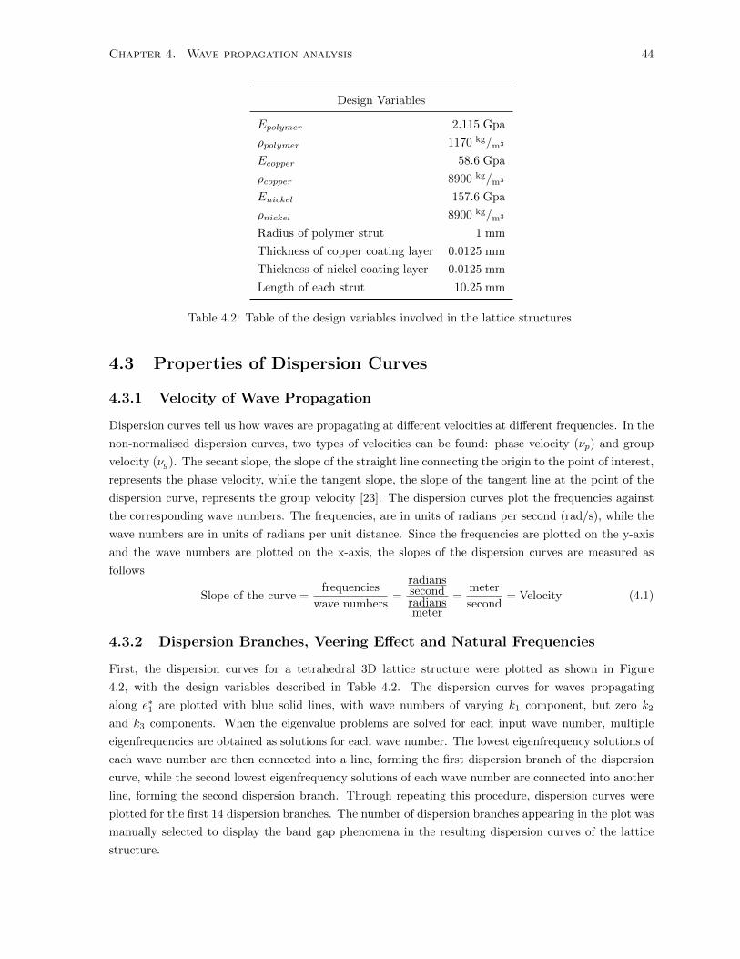
Chapter 4. Wave propagation analysis 44
Design Variables
Epolymer 2.115 Gpa
ρpolymer 1170 kg/m3
Ecopper 58.6 Gpa
ρcopper 8900 kg/m3
Enickel 157.6 Gpa
ρnickel 8900 kg/m3
Radius of polymer strut 1 mm
Thickness of copper coating layer 0.0125 mm
Thickness of nickel coating layer 0.0125 mm
Length of each strut 10.25 mm
Table 4.2: Table of the design variables involved in the lattice structures.
4.3 Properties of Dispersion Curves
4.3.1 Velocity of Wave Propagation
Dispersion curves tell us how waves are propagating at different velocities at different frequencies. In the
non-normalised dispersion curves, two types of velocities can be found: phase velocity (νp) and group
velocity (νg). The secant slope, the slope of the straight line connecting the origin to the point of interest,
represents the phase velocity, while the tangent slope, the slope of the tangent line at the point of the
dispersion curve, represents the group velocity [23]. The dispersion curves plot the frequencies against
the corresponding wave numbers. The frequencies, are in units of radians per second (rad/s), while the
wave numbers are in units of radians per unit distance. Since the frequencies are plotted on the y-axis
and the wave numbers are plotted on the x-axis, the slopes of the dispersion curves are measured as
follows
Slope of the curve =frequencies
wave numbers=
radianssecondradiansmeter
=meter
second= Velocity (4.1)
4.3.2 Dispersion Branches, Veering Effect and Natural Frequencies
First, the dispersion curves for a tetrahedral 3D lattice structure were plotted as shown in Figure
4.2, with the design variables described in Table 4.2. The dispersion curves for waves propagating
along e∗1 are plotted with blue solid lines, with wave numbers of varying k1 component, but zero k2
and k3 components. When the eigenvalue problems are solved for each input wave number, multiple
eigenfrequencies are obtained as solutions for each wave number. The lowest eigenfrequency solutions of
each wave number are then connected into a line, forming the first dispersion branch of the dispersion
curve, while the second lowest eigenfrequency solutions of each wave number are connected into another
line, forming the second dispersion branch. Through repeating this procedure, dispersion curves were
plotted for the first 14 dispersion branches. The number of dispersion branches appearing in the plot was
manually selected to display the band gap phenomena in the resulting dispersion curves of the lattice
structure.

Chapter 4. Wave propagation analysis 45
0 0.2 0.4 0.6 0.8 10
500
1000
1500
2000
2500
3000
3500
Normalised Wave Number
Fre
quen
cy (
rad/
s)
Figure 4.2: Illustration of the dispersion curves of the tetrahedral lattice with the design variables inTable 4.2.
Often, when the dispersion curves are plotted based on frequency (ordinate) against the wave vector
(abscissa), the observed dispersion branches look as if they are crossing each other. However, the
dispersion branches that seem to be crossing each other are in fact just coming close to each other, then
they make a steep change in direction at some point. In reality, the dispersion branches never cross each
other in the dispersion curve. This phenomenon is called veering [22].
0.28 0.3 0.32 0.34 0.36 0.38
1800
1850
1900
1950
2000
2050
2100
2150
2200
Normalised Wave Number
Fre
quen
cy (
rad/
s)
Figure 4.3: Illustration of the four dispersion branches experiencing the veering effect.
Paying attention to 3rd, 4th, 5th, and 6th dispersion branches of the dispersion curves, the four dispersion
branches seem as if they are crossing each other. However, as illustrated in Figure 4.3, when the plot
is magnified to display the four dispersion branches between the normalised wave numbers of 0.28 and
0.38, and the frequency range of 1800 and 2200 rad/s, it can be observed that these are in fact, four
separate dispersion branches that do not cross each other.

Chapter 4. Wave propagation analysis 46
0 0.2 0.4 0.6 0.8 12422.5
2423
2423.5
2424
2424.5
2425
Normalised Wave Number
Fre
quen
cy (
rad/
s)
Figure 4.4: Illustration of the dispersion branch representing the natural frequency of the lattice struc-ture.
Other information that can be obtained from the dispersion curves is the natural frequency of the
lattice structure. The flat dispersion branch in the middle of Figure 4.2 represents natural frequency,
the frequency at which the lattice structure tends to vibrate. As illustrated in Figure 4.4, when no
other dispersion branches are present except for the natural frequency, the natural frequency occurs at
a frequency of 2424 rad/s, representing the 11th dispersion branch.
0.516 0.518 0.52 0.522 0.524 0.526 0.528 0.53
2390
2395
2400
2405
2410
2415
2420
2425
2430
2435
2440
Normalised Wave Number
Fre
quen
cy (
rad/
s)
Figure 4.5: Illustration of multiple dispersion branches located close to each other.
While it was aforementioned that the dispersion curves illustrated in Figure 4.2 are plotted for 14
dispersion branches, the dispersion curves appear to only contain eight dispersion branches. The reason
for this is that there are multiple dispersion branches that are tightly close to each other near the
dispersion branch representing the natural frequency. Figure 4.5 provides magnified representation of
the multiple dispersion branches that are located close to each other. These dispersion branches never

Chapter 4. Wave propagation analysis 47
cross each other, and among the dispersion branches depicted in Figure 4.5, only one dispersion branch
is flat, with a uniform eigenfrequency, representing the natural frequency.
4.3.3 Band Gap Phenomenon
In the dispersion curve, if there is a gap between the dispersion branches, the gap is referred as a
band gap in solid-state physics, where no wave propagation occurs within the band gap region. In other
words, phononic waves, which are of primary interest in this thesis, will not propagate in any direction at
frequencies associated with band gaps. Figure 4.6 illustrates the band gap phenomenon and its location
in dispersion curves. A band gap appears between the 13th and 14th dispersion branches at the frequency
range of 2424-2957 rad/s, in which there are no waves propagating within this frequency range.
Figure 4.6: Illustration of the band gap in the dispersion curves of the tetrahedral lattice structure withthe design variables in Table 4.2.
4.4 Validation Through Two-dimensional Triangular Lattices
The numerical model was verified through comparing the dispersion curves generated from the numerical
model with the dispersion curves calculated by A. Phani et al. [23]. In their research, wave propagation
through a 2D triangular lattice structure with a radius to length ratio of 0.1 was performed. As their
report did not define specific values of the Young’s modulus and the density of the struts, the numerical
model in this thesis used arbitrary values of other design variables, but with matching the radius to
length ratio. First, a triangular lattice structure with a radius to length ratio of 0.1 was compared, as
shown in Figure 4.7.

Chapter 4. Wave propagation analysis 48
0 0.2 0.4 0.6 0.8 10
1000
2000
3000
4000
5000
6000
7000
8000
Normalised k−space position
Fre
quen
cy (
rad/
s)
Figure 4.7: Comparison of the dispersion curves of a 2D triangular lattice with a radius to length ratioof 0.1 through finite element analysis (left) and the dispersion curves adopted from A. Phani et al. [23](right).
The two dispersion curves show close resemblance of their band structures, with a band gap located in
the high frequency range. The first band gap of the dispersion curves occurs between the 5th and 6th
dispersion branches, while the second band gap of the dispersion curves occurs between the 6th and 7th
dispersion branches for both plots.
Next, a triangular lattice structure with a radius to length ratio of 0.02 was then compared, as il-
lustrated in Figure 4.8. The two plots show close resemblance of dispersion surfaces, with a band gap
located in the low frequency range between the 3rd and 4th dispersion surfaces from the bottom.
0 0.2 0.4 0.6 0.8 10
100
200
300
400
500
600
700
Normalised k−space position
Fre
quen
cy (
rad/
s)
Figure 4.8: Comparison of the dispersion curves of a 2D triangular lattice with a radius to length ratioof 0.02 through finite element analysis (left) and the dispersion curves adopted from A. Phani et al. [23](right).

Chapter 4. Wave propagation analysis 49
4.5 Gaining a Physical Understanding of the Lattice Structure
It is of interest to understand what happens in the physical space in a physical lattice structure when a
wave propagates along a strut of the lattice structure. For this purpose, wave vectors propagating along
the direction of the direct basis vector e1 of each tetrahedral and pyramidal lattice structure were used
as inputs for the eigenvalue problem to solve it for the eigenvectors φ.
Kφ = ω2Mφ (4.2)
The eigenvector solution of the eigenvalue problem is in the form of a matrix, with the rows of the matrix
representing nodal displacement of all the nodes existing in the lattice structure, and the columns of
the matrix representing the nodal displacements of different mode shapes. The nodal displacements
of the first mode are incorporated with the original location of the nodes of the lattice structures to
demonstrate the first mode of the deformation of the tetrahedral and pyramidal lattice structures. The
struts in light blue colour represent undeformed struts of the tetrahedral or pyramidal lattice structure,
while the struts in orange colour represent the deformed struts of the lattice structures. While the
deformation is demonstrated for the first mode, some struts have frequency of one, while some struts
exhibit a frequency of two. This can be explained by intuitively performing nodal rotations for each
node of the struts in each lattice structure. For this, first, pick a node at the end of one strut of an
undeformed structure. By performing nodal rotation on the selected node, the struts sharing this node
are expected to deform in one mode as the nodes at the other end of the strut are considered fixed.
Afterwards, move on to the remaining nodes of the lattice structure and perform nodal rotation while
trying to maintain the deformation of each strut having one mode only. By repeating this procedure, it
is impossible to keep all the struts having only a single mode. Therefore, it is inevitable that there will
be at least one strut with two modes.
Figure 4.9: Illustration of the first mode deformation of a tetrahedral lattice structure for waves propa-gating along strut A (along the direct basis vector e1).

Chapter 4. Wave propagation analysis 50
Figure 4.10: Illustration of the first mode deformation of a pyramidal lattice structure for waves propa-gating along strut A (along the direct basis vector e1).
4.6 Wave Propagation Through a Tetrahedral Lattice Structure
with a Radius to Length Ratio of 0.1
In this section, the wave propagation behaviour of a 3D tetrahedral lattice structure with a radius to
length ratio of 0.1 is analyzed. First, the wave propagation behaviour through the symmetric lattice
structure was examined, in which all the struts of the structure have equal design variables, such as
radius and length of the lattice struts, thickness of the coating layers, and materials used for the struts
and coating layers. Afterwards, wave propagation behaviour through the non-symmetric lattice structure
was analyzed, in which one or more struts of the structure had modified design variables. The dispersion
curves were plotted for the frequencies of wave propagation for the corresponding wave vectors propagat-
ing in the direction of the reciprocal basis vector e∗1 (wave vector with a varying k1 component, while the
k2 and k3 components are zero), and another dispersion curves were plotted for the waves propagating
in the direction of the reciprocal basis vector e∗2 (wave vector with a varying k2 component, while the
k1 and k3 components are zero). Analysis of the non-symmetric lattice was performed to measure the
symmetric and asymmetric dispersion relation behaviours in the non-symmetric lattice structures. Also,
analysis of the different combinations of modified struts were performed to measure the changes in the
resulting dispersion curves. Moreover, analysis of the non-symmetric lattice was performed whereby the
total number of modified struts of the lattice structure were increased gradually, in order to identify
the impact of such changes on the band structures of the dispersion curves. The wave numbers of the
resulting dispersion curves were normalized.
4.6.1 Initial Symmetric Lattice Structure
Dispersion curves of the initial symmetric tetrahedral lattice structure with a radius to length ratio of
0.1 are illustrated in Figure 4.11. All the struts of the unit cell share the same design variables defined
previously in Table 4.2. Dispersion curves are plotted for waves propagating in two different directions.
The dispersion curves for waves propagating along e∗1 are plotted with blue dotted lines, while the
dispersion curves for waves propagating along e∗2 are plotted with red solid lines. The dispersion curves
are plotted for first 14 dispersion branches, in which the number of the displayed dispersion branches

Chapter 4. Wave propagation analysis 51
are predefined to present the band gap phenomena in the resulting dispersion curves.
0 0.2 0.4 0.6 0.8 10
500
1000
1500
2000
2500
3000
3500
Normalised Wave Number
Fre
quen
cy (
rad/
s)
Figure 4.11: Dispersion curve of a symmetric tetrahedral lattice with a r:l ratio of 0.1 for waves propa-gating along e∗1 (blue dotted lines) and for waves propagating along e∗2 (red solid lines).
First, as the definition of the dispersion curves illustrates, the plot provides information on how waves
propagate at different frequencies in different phase velocities and group velocities. The phase velocity
of a point can be obtained by connecting a straight line between the origin and the point of interest,
then find the slope of the straight line. On the other hand, the group velocity of the point can be
obtained by forming a line tangent to the point on the curve, and then taking the slope of the tangent
line. For example, for the first dispersion branch, phase velocities and group velocities of each waves
were measured and are plotted below to demonstrate how waves propagate at different speeds as the
wave numbers of wave vectors are gradually increased (or as the wave length of the wave vectors are
gradually reduced).
0 0.2 0.4 0.6 0.8 10
0.5
1
1.5
2
2.5
3
3.5
4
4.5
5
Normalised Wave Number
Pha
se V
eloc
ity (
km/s
)
0 0.2 0.4 0.6 0.8 1−5
−4
−3
−2
−1
0
1
2
3
4
5
Normalised Wave Number
Gro
up V
eloc
ity (
km/s
)
Figure 4.12: Phase velocity (left) and group velocity (right) of the first dispersion branch for wavespropagating along e∗1 (blue dotted lines) and for waves propagating along e∗2 (red solid lines).

Chapter 4. Wave propagation analysis 52
As the plots illustrate, with the increasing wave number of the wave vectors (i.e. decreasing wave length),
the phase velocity of the corresponding wave numbers are gradually decreased from 4.721 km/s to 0.0184
km/s. On the other hand, the group velocity of the first dispersion branch gradually decreases from a
positive 4.721 km/s, reaching zero velocity at a normalised wave number of 0.5. However, beyond this
point, the group velocity goes into the negative region, while the magnitude of the velocity begins to
increase. This change from a positive to a negative region implies a change in the direction of the group
velocity relative to the phase velocity. When the group velocity is in a positive region, the group velocity
is moving in the same direction as the phase velocity. However, when the group velocity is in a negative
region, the group velocity is moving in the opposite direction to the phase velocity.
0 0.2 0.4 0.6 0.8 10
50
100
150
200
250
300
350
400
Normalised Wave Number
Pha
se V
eloc
ity (
km/s
)
0.05 0.1 0.15 0.2 0.250
10
20
30
40
50
60
70
80
90
100
Normalised Wave Number
Pha
se V
eloc
ity (
km/s
)
Figure 4.13: Phase velocity plot of the first 14 dispersion branches (left), and a close look of the plot atsmall wave numbers (right).
The phase velocities for all 14 dispersion branches are plotted in Figure 4.13. The left plot shows the
change in phase velocity over all the ranges of wave numbers, while the right plot shows the change in
phase velocity over the ranges of the normalised wave numbers from 0 to 0.25. Compared to the first
four dispersion branches, in which the waves with small wave numbers propagate in the low frequency
range, the remaining dispersion branches propagate at much higher frequencies for the same correspond-
ing wave numbers. Therefore, the 5th and higher dispersion branches show the phase velocities decaying
exponentially as the wave numbers increase.
The second significant information that the dispersion curves provide is information on the band gap
phenomenon and its location. A band gap appears between the 13th and 14th dispersion branches at
the frequency range of 2424-2957 rad/s, in which contains no waves propagating within this frequency
range. For the initial symmetric tetrahedral lattice structure, the dispersion relations of the waves prop-
agating in the direction of the reciprocal basis vector e∗1 are equal to the dispersion relations of the waves
propagating in the direction of the reciprocal basis vector e∗2, thus demonstrating symmetric behaviours.
Hence, the dispersion curves and the band gaps overlap with each other.
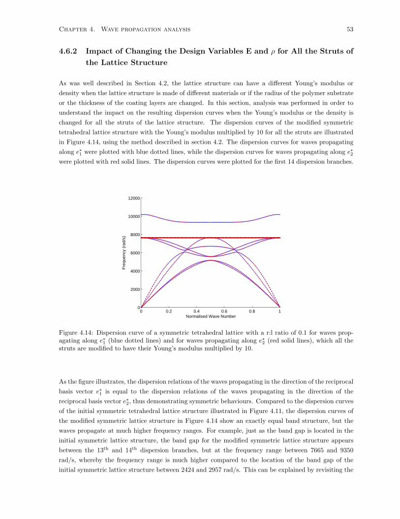
Chapter 4. Wave propagation analysis 53
4.6.2 Impact of Changing the Design Variables E and ρ for All the Struts of
the Lattice Structure
As was well described in Section 4.2, the lattice structure can have a different Young’s modulus or
density when the lattice structure is made of different materials or if the radius of the polymer substrate
or the thickness of the coating layers are changed. In this section, analysis was performed in order to
understand the impact on the resulting dispersion curves when the Young’s modulus or the density is
changed for all the struts of the lattice structure. The dispersion curves of the modified symmetric
tetrahedral lattice structure with the Young’s modulus multiplied by 10 for all the struts are illustrated
in Figure 4.14, using the method described in section 4.2. The dispersion curves for waves propagating
along e∗1 were plotted with blue dotted lines, while the dispersion curves for waves propagating along e∗2
were plotted with red solid lines. The dispersion curves were plotted for the first 14 dispersion branches.
0 0.2 0.4 0.6 0.8 10
2000
4000
6000
8000
10000
12000
Normalised Wave Number
Fre
quen
cy (
rad/
s)
Figure 4.14: Dispersion curve of a symmetric tetrahedral lattice with a r:l ratio of 0.1 for waves prop-agating along e∗1 (blue dotted lines) and for waves propagating along e∗2 (red solid lines), which all thestruts are modified to have their Young’s modulus multiplied by 10.
As the figure illustrates, the dispersion relations of the waves propagating in the direction of the reciprocal
basis vector e∗1 is equal to the dispersion relations of the waves propagating in the direction of the
reciprocal basis vector e∗2, thus demonstrating symmetric behaviours. Compared to the dispersion curves
of the initial symmetric tetrahedral lattice structure illustrated in Figure 4.11, the dispersion curves of
the modified symmetric lattice structure in Figure 4.14 show an exactly equal band structure, but the
waves propagate at much higher frequency ranges. For example, just as the band gap is located in the
initial symmetric lattice structure, the band gap for the modified symmetric lattice structure appears
between the 13th and 14th dispersion branches, but at the frequency range between 7665 and 9350
rad/s, whereby the frequency range is much higher compared to the location of the band gap of the
initial symmetric lattice structure between 2424 and 2957 rad/s. This can be explained by revisiting the

Chapter 4. Wave propagation analysis 54
expression for the mass matrix and stiffness matrix derived in the previous chapter.
mij =
L∫0
[Aρ(aiaj + bibj + cicj) + Iyρeiej + Izρfifj + (Iy + Iz)ρdidj
]dx (4.3)
kij =
L∫0
[λ(Aa′ia
′j + Iye
′ie′j + Izf
′if′j) + 2G(Aa′ia
′j + Iye
′ie′j + Izf
′if′j)
+ κGA(
(b′i − fi)(b′j − fj) + (c′i + ei)(c′j + ej)
)+ κG(Iz + Iy)(d′id
′j)]dx (4.4)
where mij is the mass matrix of an individual strut in a global coordinate system and kij is the stiffness
matrix of an individual strut in a global coordinate system. If the radius and length of the struts remain
constant, the density ρ becomes the only variable in the equation of the mass matrix. Therefore, when
the radius and length of the strut are fixed, the mass matrix of a strut can be re-expressed as
mij = ρ
L∫0
[A(aiaj + bibj + cicj) + Iyeiej + Izfifj + (Iy + Iz)didj
]dx = ρm′ij (4.5)
where
m′ij =
L∫0
[A(aiaj + bibj + cicj) + Iyeiej + Izfifj + (Iy + Iz)didj
]dx (4.6)
In the stiffness matrix equation, the design variables λ, G, and E are involved. However, as the shear
modulus and Young’s modulus are related,
G =E
2(1 + ν)(4.7)
and since Lame’s first parameter is related with the shear modulus and Young’s modulus:
λ =G(E − 2G)
3G− E(4.8)
where λ and G can be expressed in terms of E, and the stiffness matrix equation can be re-expressed as
follows:
kij = E
L∫0
[(Aa′ia
′j + Iye
′ie′j + Izf
′if′j) + (Aa′ia
′j + Iye
′ie′j + Izf
′if′j)
+(
(b′i − fi)(b′j − fj) + (c′i + ei)(c′j + ej)
)+ (Iz + Iy)(d′id
′j)]dx = Ek′ij (4.9)
The collection of mass and stiffness matrices of the individual struts (A,B,C,D,E, F ) to form the mass
and stiffness matrices of the entire structure in the global coordinate system (Mls, Kls) can be expressed
as
Mls = (mA +mB +mC +mD +mE +mF ) = ρm′A + ρm′B + ρm′C + ρm′D + ρm′E + ρm′F (4.10)

Chapter 4. Wave propagation analysis 55
Kls = (kA + kB + kC + kD + kE + kF ) = Ek′A + Ek′B + Ek′C + Ek′D + Ek′E + Ek′F (4.11)
For a symmetric lattice structure, an equal value of the Young’s modulus or the density is applied for
each individual strut. Since the remaining terms of the mass matrix and stiffness matrix equations
remain constant for all the struts, and are independent from the change in ρ and E, the global mass and
stiffness matrices of the entire structure can be expressed as
Mls = ρM ′ls (4.12)
where,
M ′ls = m′A +m′B +m′C +m′D +m′E +m′F (4.13)
and
Kls = EK ′ls (4.14)
where,
K ′ls = k′A + k′B + k′C + k′D + k′E + k′F (4.15)
This relationship can be extended to the reduced global mass and stiffness matrices.
Mls = ρM ′ls (4.16)
Kls = EK ′ls (4.17)
Applying the above relations, the eigenvalue problem for the initial symmetric lattice structure can be
expressed as
E1K ′1φ = ω21ρ1M
′1φ (4.18)
while, the eigenvalue problem for the modified symmetric lattice structure can be expressed as
E2K ′2φ = ω22ρ2M
′2φ (4.19)
Knowing that the mass and stiffness matrices, K ′ and M ′ , for both the initial symmetric lattice structure
and the modified symmetric lattice structure are equal only when the Young’s modulus or the density
is changed for all the struts,
K ′1 = K ′2 = K ′ (4.20)
M ′1 = M ′2 = M ′ (4.21)
then, the relationship between the two eigenvalue problems can be equated as follows:
E1K ′φ = ω21ρ1M
′φ (4.22)
E2K ′φ = ω22ρ2M
′φ (4.23)
Equating the above two equations,ω22
E2
ρ2
=ω21
E1
ρ1
(4.24)

Chapter 4. Wave propagation analysis 56
Re-ordering Equation 4.24,
ω2 = ω1
√E2ρ1E1ρ2
(4.25)
Hence, the relationship between the initial and the modified symmetric lattice structures, when the
Young’s modulus and/or the density of all the struts are modified, can be expressed by a scalar factor
of the ratio between the Young’s modulus and the density.√ratio of E
ratio of ρ(4.26)
This relationship can be verified through comparison of the locations of the band gaps between the initial
and modified symmetric lattice structures in the above example, in which the Young’s modulus of the
modified symmetric lattice structure is multiplied by a factor of 10 while the density is unchanged.
ρ2 = ρ1 (4.27)
E2 = 10E1 (4.28)
It is expected that the dispersion curve of the modified symmetric lattice structure will be scaled by a
factor of√
10, at which eigenfrequencies of all wave numbers of the dispersion curves are multiplied by
the same factor of√
10, compared to the dispersion curve of the initial symmetric lattice structure. When
the initial lattice structure has a band gap in the frequency range of 2424-2957 rad/s, the frequency range
at which the band gap of the modified symmetric lattice will appear can be calculated by multiplying
by this factor at each the lower bound and upper bound of the frequency range at which the band gap
appeared in the initial lattice structure.
Lower bound in second dispersion curve = 2424×√
10 = 7665
Upper bound in second dispersion curve = 2957×√
10 = 9350(4.29)
Through the above relation, the frequency range at which the band gap will appear for the modified
symmetric lattice structure is expected to be at 7665-9350 rad/s, which matches with the result from
the finite element analysis. Therefore, in symmetric lattice structures, changing the value of the Young’s
modulus and/or the density simply scales the dispersion curve by factor of√
Eρ , This relation can be
applied to any 2D lattice structure as well as to any 3D lattice structure with any design variables as
long as the lattice structures are symmetric and only the Young’s modulus and the density are changed.
The above relation plays an important role when tailoring the band gap location of the dispersion
curves. Based on the expression, increasing the Young’s modulus or reducing the density using the
method described in Section 4.2 provides dispersion curves with the same band structure, but with
waves propagating at a higher frequency range, which the frequency ranges and the band gap location is
multiplied by a factor of√
Eρ . On the other hand, reducing Young’s modulus or increasing the density
provides dispersion curves with the same band structure, but with waves propagating at reduced fre-
quency ranges. Therefore, when a band gap is present in the dispersion curves of the lattice structure,
but is desired to be placed at a different frequency range, Young’s modulus can be changed by main-
taining the radius of the polymer substrate and the overall strut radius, while only modifying the ratio

Chapter 4. Wave propagation analysis 57
of the thickness of the two coating layers to achieve such a requirement. However, while this relation
may seem strong and an easy method to tailor the band gap location, it holds one factor that may be
considered a weakness. As this relation simply scales the entire dispersion curve by the factor derived
above, it also scales the frequency range at which the band gap occurs. Therefore, not only does this
relation shift the location of the band gap, but it also increases or decreases the size of the band gap,
which may be an unintentional consequence.
4.6.3 Impact of Changing the Design Variables E and ρ for a Non-Symmetric
Lattice Structure
Strut A Modified
Next, the wave propagation behaviour in non-symmetric lattice structures was studied to analyze the
differences in dispersion relations compared to in the symmetric lattice structures. The non-symmetric
lattice structures were created by modifying the design variables of one or more, but not all the struts of
the unit lattice cell. First, strut A, which was oriented along the direct basis vector e1, was modified to
have its Young’s modulus multiplied by 10, while the other five struts remained unchanged. As Figure
4.15 illustrates, the dispersion curves of the wave propagating along e∗1 (blue dotted lines in the left
plot) and the dispersion curves of the wave propagating along e∗2 (red dotted lines in the right plot) were
plotted and compared with the dispersion curves of the initial symmetric lattice structure (black solid
lines in both plots).
0 0.2 0.4 0.6 0.8 10
500
1000
1500
2000
2500
3000
3500
4000
4500
5000
Normalised Wave Number
Fre
quen
cy (
rad/
s)
0 0.2 0.4 0.6 0.8 10
500
1000
1500
2000
2500
3000
3500
4000
4500
Normalised Wave Number
Fre
quen
cy (
rad/
s)
Figure 4.15: Dispersion curves of the non-symmetric tetrahedral lattice structure for waves propagatingalong e∗1 (blue dotted lines in the left plot) and for waves propagating along e∗2 (red dotted lines in theright plot), with strut A modified to have increased Young’s modulus by 10 times, compared with thedispersion curves of the initial symmetric lattice structure shown in Figure 4.11 (black solid lines in bothplots)
The dispersion curves for waves propagating along e∗1 were plotted with blue dotted lines, and the disper-
sion curves for waves propagating along e∗2 were plotted in red dotted lines, while the dispersion curves of
the initial symmetric lattice analyzed in Figure 4.11 were plotted with black solid lines. The dispersion
curves are plotted for the first 14 dispersion branches. Starting with the dispersion curves of the waves
propagating along e∗1, it can be seen that as one of the struts was modified to have a higher stiffness, the

Chapter 4. Wave propagation analysis 58
waves propagate at much higher frequency ranges. In the initial symmetric lattice structure, the first
14 dispersion branches show waves propagating within the frequency ranges of 39.74-3224 rad/s. How-
ever, for the non-symmetric lattice structure, the first 14 dispersion branches show waves propagating
up to the frequency range of 4858 rad/s. Also, waves of each individual dispersion branch of the non-
symmetric lattice structure propagate at a higher frequency range compared to the corresponding waves
of each of the dispersion branches of the initial symmetric lattice structure, implying the waves of the
non-symmetric lattice structures propagate at a higher phase velocity than the waves of the initial sym-
metric lattice structures. The dispersion curves of the waves propagating along e∗2 of the non-symmetric
lattice show a similar phenomenon. As the first 14 dispersion branches show waves propagating up
to the frequency range of 4255 rad/s, the waves propagate at much higher frequency than the waves
propagating through the initial symmetric lattice structure. Also, for each dispersion branch, waves in
non-symmetric lattice structure propagate at a higher frequency than the waves in the corresponding
dispersion branches in symmetric lattice structure, showing that the waves in the non-symmetric lattice
structure propagate with a higher phase velocity than the waves in the symmetric lattice structure. In
terms of the band gap phenomenon, there is no complete band gap for waves propagating along e∗1, but
there exists one band gap for waves propagating along e∗2 in the frequency range of 2483-2597 rad/s.
The first significant difference between the dispersion relations of the waves propagating in the above
non-symmetric lattice structure and the initial symmetric lattice structure comes from the difference in
the band structure. In the previous section, when the initial symmetric lattice structure was modified
so that all the struts of the lattice structures would have an increased Young’s modulus, it was observed
that the band structures remained the same and the dispersion curves were simply scaled by a certain
factor. However, when only one strut was modified to have an increased Young’s modulus, the scalar
relation did not apply, thereby leading to different band structures in the dispersion curves. This can
be explained by re-visiting the energy equations involving the mass and stiffness matrices. While a
symmetric lattice structure defines that the change in design variables are applied to all the struts in
the lattice structure, a non-symmetric lattice structure implies that only one or a few struts (but not
all) of the lattice structure have their design variables changed. Thus at first, when Young’s modulus or
the density is changed in a symmetric lattice structure, a change in the design variable is also applied
to every strut of the lattice structure.
M1 = (m1A+m1B +m1C +m1D+m1E +m1F ) = ρm′1A+ρm′1B +ρm′1C +ρm′1D+ρm′1E +ρm′1F (4.30)
K1 = (k1A + k1B + k1C + k1D + k1E + k1F ) = Ek′1A + Ek′1B + Ek′1C + Ek′1D + Ek′1E + Ek′1F (4.31)
As the terms involving the shape functions, m′ and k′, remain constant for all the struts, and as the
terms are independent from the change in ρ, the global mass matrix of the symmetric structure can be
expressed as
M1 = ρM ′1 (4.32)
K1 = EK ′1 (4.33)
where,
M ′1 = m′1A +m′1B +m′1C +m′1D +m′1E +m′1F (4.34)
K ′1 = k′1A + k′1B + k′1C + k′1D + k′1E + k′1F (4.35)

Chapter 4. Wave propagation analysis 59
However, when a change in the Young’s modulus or the density is only applied to a single strut, strut
A, this turns the lattice into a non-symmetric lattice structure,
M2 = (m2A+m2B+m2C+m2D+m2E+m2F ) = 10ρm′2A+ρm′2B+ρm′2C+ρm′2D+ρm′2E+ρm′2F (4.36)
K2 = (k2A + k2B + k2C + k2D + k2E + k2F ) = 10Ek′2A +Ek′2B +Ek′2C +Ek′2D +Ek′2E +Ek′2F (4.37)
reducing the equation, it becomes
M2 = ρM ′2 = ρ(10m′2A +m′2B +m′2C +m′2D +m′2E +m′2F ) (4.38)
K2 = EK ′2 = E(10k′2A + k′2B + k′2C + k′2D + k′2E + k′2F ) (4.39)
where,
M ′2 = (10m′2A +m′2B +m′2C +m′2D +m′2E +m′2F ) (4.40)
K ′2 = (10k′2A + k′2B + k′2C + k′2D + k′2E + k′2F ) (4.41)
Hence, M ′1 and K ′1 are not equal to M ′2 and K ′2, and these mass and stiffness matrices of the two dif-
ferent lattice structures cannot be expressed by a scalar (multiplicative by the factor of ratio of√
Eρ )
relationship anymore. Therefore, when applying different values of design variables, such as Young’s
modulus or density on the non-symmetric lattice structure, a different band structure is expected in the
resulting dispersion curves compared to the band structure of the symmetric lattice structure.
The second significant observation is the difference in the dispersion relations between waves propa-
gating in different directions. As Figure 4.16 illustrates, the dispersion curves of waves propagating
along e∗1 and the dispersion curves of waves propagating along e∗2 are different, and show asymmetric
dispersion relations. The dispersion curves for waves propagating along e∗1 were plotted with blue dotted
lines, and the dispersion curves for waves propagating along e∗2 were plotted with red solid lines.
0 0.2 0.4 0.6 0.8 10
500
1000
1500
2000
2500
3000
3500
4000
4500
5000
Normalised Wave Number
Fre
quen
cy (
rad/
s)
Figure 4.16: Collapsed dispersion curves of a non-symmetric tetrahedral lattice structure for wavespropagating along e∗1 (blue dotted lines) and for waves propagating along e∗2 (red solid lines), with strutA modified to have increased Young’s modulus by 10 times.

Chapter 4. Wave propagation analysis 60
As described in the previous chapter, Bloch theorem can be applied to describe displacements of all the
nodes of the unit lattice cell, to be expressed by the displacements of the internal and the basis nodes.
To achieve this, a transformation matrix was created. The transformation matrix is in the form of
T =
[I
τ
](4.42)
The top part of the transformation matrix is related to the internal and the basis nodes, and is simply
an n×n identity matrix, where n is the total number of internal and basis nodes. On the other hand, the
bottom part of the transformation matrix (τ) is related to the boundary nodes, which is in the following
form:
τ =
0 0 0 · · · 0 0 0 ek1 0 0 0 0 0
0 0 0 · · · 0 0 0 0 ek1 0 0 0 0
0 0 0 · · · 0 0 0 0 0 ek1 0 0 0
0 0 0 · · · 0 0 0 0 0 0 ek1 0 0
0 0 0 · · · 0 0 0 0 0 0 0 ek1 0
0 0 0 · · · 0 0 0 0 0 0 0 0 ek1
0 0 0 · · · 0 0 0 ek2 0 0 0 0 0
0 0 0 · · · 0 0 0 0 ek2 0 0 0 0
0 0 0 · · · 0 0 0 0 0 ek2 0 0 0
0 0 0 · · · 0 0 0 0 0 0 ek2 0 0
0 0 0 · · · 0 0 0 0 0 0 0 ek2 0
0 0 0 · · · 0 0 0 0 0 0 0 0 ek2
0 0 0 · · · 0 0 0 ek3 0 0 0 0 0
0 0 0 · · · 0 0 0 0 ek3 0 0 0 0
0 0 0 · · · 0 0 0 0 0 ek3 0 0 0
0 0 0 · · · 0 0 0 0 0 0 ek3 0 0
0 0 0 · · · 0 0 0 0 0 0 0 ek3 0
0 0 0 · · · 0 0 0 0 0 0 0 0 ek3
(4.43)
From the above matrix, k1, k2, and k3 are three components (wave numbers) of a wave vector. For
waves propagating along e∗1, k1 varies, while k2 and k3 are fixed as zero; whereas, for waves propagating
along e∗2, k2 varies, while k1 and k3 are fixed as zero. Therefore, the transformation matrix for waves
propagating in the e∗1 direction and e∗2 direction are different. Then the transformation matrices are
multiplied to the global mass and stiffness matrices to create reduced global mass and stiffness matrices,
where TH is the conjugate transpose of the transformation matrix,
THMT = M (4.44)
THKT = K (4.45)
since the transformation matrices for waves propagating along e∗1 are different to those from e∗2, there
exists two different sets of reduced mass and stiffness matrices. However, as illustrated in Figures 4.11
and 4.14, when the eigenvalue problems are solved for the symmetric lattice structures with the different
sets of reduced mass and stiffness matrices, symmetric eigen solutions can be obtained for waves propa-
gating in the e∗1 and e∗2 directions. On the other hand, as illustrated in Figure 4.16, when the eigenvalue

Chapter 4. Wave propagation analysis 61
problems are solved for a non-symmetric lattice structure with strut A modified to have higher stiffness,
asymmetric solutions are obtained for waves propagating in the e∗1 and e∗2 directions. This difference in
symmetric/asymmetric dispersion curves is related to the geometrical symmetry of the lattice structure
and how the modification of the design variables impacts on the symmetry with respect to each direction
of wave propagation. First, recall the orientation of the tetrahedral unit lattice cell in Cartesian coor-
dinates illustrated in Figure 4.17 (left); with a certain rotation of the unit cell, as illustrated in Figure
4.17 (right), the tetrahedral unit cell can be viewed as symmetric with respect to the plane created by
the y-axis and direct basis vector e3 (the red line in Figure 4.15 b), in which the right region involving
e∗1 is symmetric to the left region involving e∗2.
Figure 4.17: Illustration of the symmetric view on a tetrahedral unit cell with respect to e∗1 and e∗2.
Next, consider two waves, with one wave propagating along e∗1, and another wave propagating along
e∗2. For symmetric lattice structures, in which all the struts of the lattice structure are modified equally
and are geometrically symmetric, the dispersion relation of the wave propagating along e∗1 is symmetric
to the dispersion relation of the wave propagating along e∗2. On the other hand, for a non-symmetric
lattice structure, in which only strut A is modified, due to the modification on one strut, the lattice unit
cell is no longer geometrically symmetric with respect to each direction of wave propagation. Therefore,
the dispersion relation of the wave propagating along e∗1 is asymmetric to the dispersion relation of the
wave propagating along e∗2, also with different dispersion curves and band structures. As emphasized
at the beginning of this chapter, it is important to make clear understanding of the differences between
symmetric/non-symmetric lattice structures and symmetric/asymmetric dispersion relations. A sym-
metric lattice structure refers to a structure, in which all the struts have equal design variables, while
a non-symmetric lattice structure refers to a structure, in which one or more but not all of struts are
modified to have different design variables. On the other hand, the dispersion relation is symmetric when
the resulting dispersion curves of the wave propagating in one direction are identical to the dispersion
curves of a wave propagating in a different direction, and the dispersion relation is asymmetric when the
resulting dispersion curves of a wave propagating in one direction is different from the dispersion curves
of a wave propagating in a different direction. To carry out deeper analysis and better characterization
of the asymmetric dispersion relations of non-symmetric lattice structures, three cases are considered

Chapter 4. Wave propagation analysis 62
here: a) a non-symmetric lattice structure, where modifications applied with respect to the e∗1 direction,
are applied on the struts located geometrically symmetric with respect to the e∗2 direction instead; b) a
non-symmetric lattice structure where modifications to the lattice structure are applied on struts located
geometrically symmetric with respect to both directions of the wave propagation; c) a non-symmetric
lattice structure where modifications of the design variables are concentrated on one side of the lattice
structure, and the location of the modifications applied are geometrically non-symmetric with respect
to each direction of the wave propagation.
Non-Symmetric Lattice Structure, Where the Modifications Applied with respect to the
e∗1 Direction, is Applied Equally with respect to the e∗2 Direction Instead
The first case involved observation of the impact of modifying different struts, where the previous
modification was applied with respect to the e∗1 direction of the wave propagation, but is now applied
at the strut placed at the geometrically symmetric location with respect to the e∗2 direction of the wave
propagation. In other words, in the previous case, strut A was modified and the waves were propagating
along e∗1 and e∗2. In the current section, the focus was made to analyze and compare the dispersion curve
when strut B was modified instead, and to measure the dispersion relations of the waves propagating
along e∗1 and e∗2 directions, as illustrated in Figure 4.18.
Figure 4.18: Illustration of strut A of tetrahedral unit cell modified (left) and strut B of tetrahedral unitcell modified (right). The modified strut is in orange colour.
The dispersion curves of the non-symmetric lattice structure, in which strut B was modified are plotted
in Figure 4.19 below. As discussed in the previous section, since the modification applied to the lattice
structure is geometrically non-symmetric with respect to each direction of the wave propagation, the
dispersion relations between the waves propagating along e∗1 and e∗2 are asymmetric. The dispersion
curves for waves propagating along e∗1 was plotted with blue dotted lines, while the dispersion curves for
waves propagating along e∗2 was plotted with red solid lines.

Chapter 4. Wave propagation analysis 63
0 0.2 0.4 0.6 0.8 10
500
1000
1500
2000
2500
3000
3500
4000
4500
5000
Normalised Wave Number
Fre
quen
cy (
rad/
s)
Figure 4.19: Collapsed dispersion curves of a non-symmetric tetrahedral lattice structure for wavespropagating along e∗1 (blue dotted lines) and for waves propagating along e∗2 (red solid lines), with strutA modified to have increased Young’s modulus by 10 times.
When the above dispersion curves are compared with the dispersion curves of waves propagating through
the non-symmetric lattice structure when strut A is modified, as illustrated in Figure 4.16, it can be
seen that the band structures of the dispersion curves are identical. However, as Figure 4.20 illustrates,
the dispersion curves of waves propagating along e∗2 of the non-symmetric lattice structure with strut
B modified, are symmetric with the dispersion curves of the waves propagating along e∗1 of the non-
symmetric lattice structure with strut A modified. Likewise, the dispersion curves of waves propagating
along e∗1 of the non-symmetric lattice structure with strut B modified, are symmetric with the dispersion
curves of the waves propagating along e∗2 of the non-symmetric lattice structure with strut A modified.
The dispersion curves from Figure 4.16 are plotted with blue dotted lines, and the current dispersion
curves are plotted with red solid lines.
0 0.2 0.4 0.6 0.8 10
500
1000
1500
2000
2500
3000
3500
4000
4500
5000
Normalised Wave Number
Fre
quen
cy (
rad/
s)
0 0.2 0.4 0.6 0.8 10
500
1000
1500
2000
2500
3000
3500
4000
4500
Normalised Wave Number
Fre
quen
cy (
rad/
s)
Figure 4.20: Comparisons of the dispersion curves for waves propagating along e∗1 when strut A ismodified (blue dotted lines on the left) and for waves propagating along e∗2 when strut B is modified(red solid lines on the left) and the dispersion curves for waves propagating along e∗2 when strut A ismodified (blue dotted lines on the right) and for waves propagating along e∗1 when strut B is modified(red solid lines on the right).
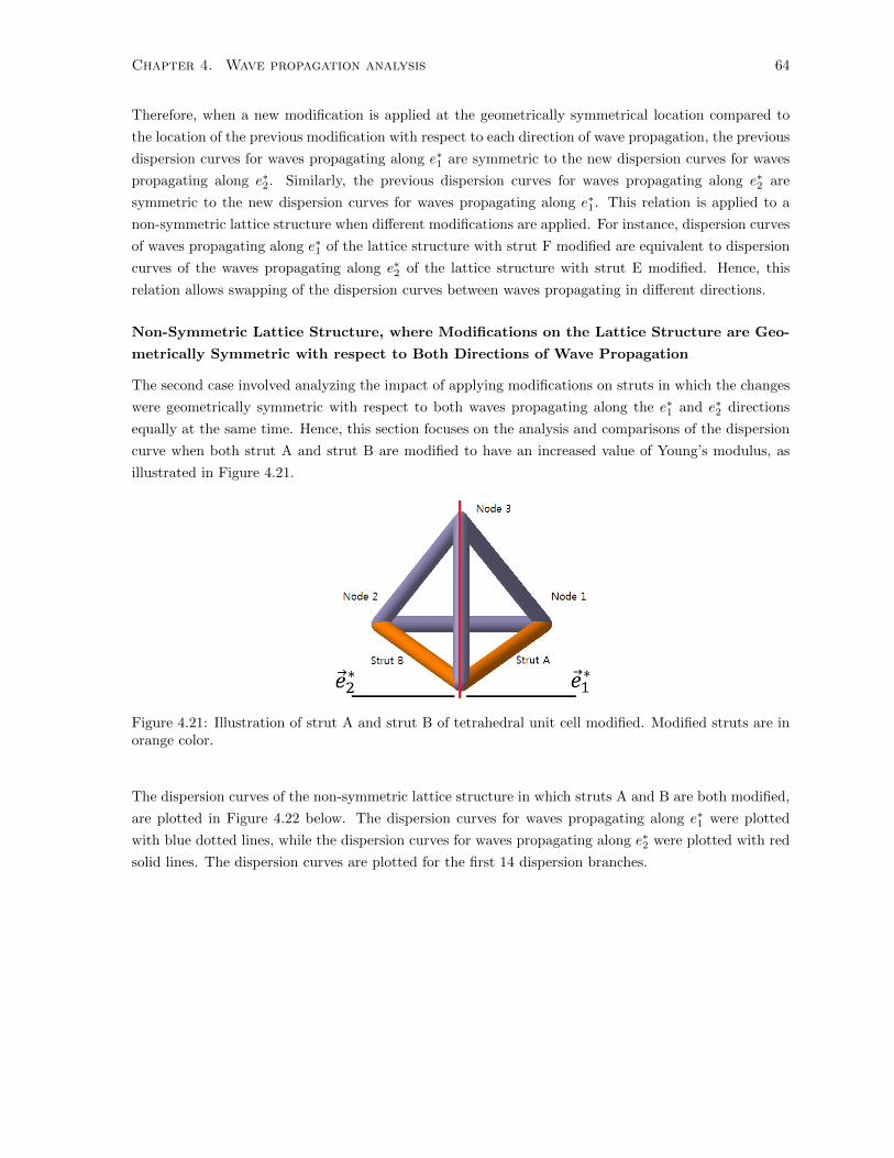
Chapter 4. Wave propagation analysis 64
Therefore, when a new modification is applied at the geometrically symmetrical location compared to
the location of the previous modification with respect to each direction of wave propagation, the previous
dispersion curves for waves propagating along e∗1 are symmetric to the new dispersion curves for waves
propagating along e∗2. Similarly, the previous dispersion curves for waves propagating along e∗2 are
symmetric to the new dispersion curves for waves propagating along e∗1. This relation is applied to a
non-symmetric lattice structure when different modifications are applied. For instance, dispersion curves
of waves propagating along e∗1 of the lattice structure with strut F modified are equivalent to dispersion
curves of the waves propagating along e∗2 of the lattice structure with strut E modified. Hence, this
relation allows swapping of the dispersion curves between waves propagating in different directions.
Non-Symmetric Lattice Structure, where Modifications on the Lattice Structure are Geo-
metrically Symmetric with respect to Both Directions of Wave Propagation
The second case involved analyzing the impact of applying modifications on struts in which the changes
were geometrically symmetric with respect to both waves propagating along the e∗1 and e∗2 directions
equally at the same time. Hence, this section focuses on the analysis and comparisons of the dispersion
curve when both strut A and strut B are modified to have an increased value of Young’s modulus, as
illustrated in Figure 4.21.
Figure 4.21: Illustration of strut A and strut B of tetrahedral unit cell modified. Modified struts are inorange color.
The dispersion curves of the non-symmetric lattice structure in which struts A and B are both modified,
are plotted in Figure 4.22 below. The dispersion curves for waves propagating along e∗1 were plotted
with blue dotted lines, while the dispersion curves for waves propagating along e∗2 were plotted with red
solid lines. The dispersion curves are plotted for the first 14 dispersion branches.

Chapter 4. Wave propagation analysis 65
0 0.2 0.4 0.6 0.8 10
500
1000
1500
2000
2500
3000
3500
4000
4500
5000
Normalised Wave Number
Fre
quen
cy (
rad/
s)
Figure 4.22: Collapsed dispersion curves of a non-symmetric tetrahedral lattice structure for wavespropagating along e∗1 (blue dotted lines) and for waves propagating along e∗2 (red solid lines), with strutsA and B modified to have increased Young’s modulus by 10 times.
One distinct change compared to the previous experiment is the symmetric dispersion relations between
waves propagating in the e∗1 and e∗2 directions. In the previous experiment case, in which only either strut
A or strut B was modified, the dispersion curves of the waves propagating in two different directions were
asymmetric. The asymmetric solutions were a result of the modifications made on the lattice structure
not being geometrically symmetric with respect to each direction of wave propagation. However, when
both strut A and B were modified, the modification applied on the lattice structure was symmetric with
respect to both directions of wave propagation, resulting in the symmetric dispersion relations between
waves propagating along e∗1 and e∗2. This relationship could be extended to other non-symmetric lattice
structures with different modifications, in which the modifications applied are geometrically symmetric
with respect to waves propagating in different directions. For instance, modifying struts A, B, and C all
together would result in symmetric dispersion relations as the modifications applied are geometrically
symmetric with respect to both directions of the wave propagation. It is important to note that when
struts are modified, the same changes in the design variables are applied for the modified struts.
4.6.4 Impact of Modifying Different Combinations of Struts of the Lattice
Structure
In the previous experiments on non-symmetric lattice structures, the relationship between the location
of the modifications and the symmetric/asymmetric dispersion relations were discussed. In this section,
in order to explore how various different asymmetric relations can be obtained, and to further analyze
the significance of having asymmetric dispersion relations for waves propagating in different directions,
the thesis focuses on modifications skewed to one location, in which case the modifications applied on
the struts would impact one side of the unit lattice structure, while affecting the other side of the unit
lattice structure as little as possible. In this section and onward, the modifications are applied to impact
node 1, the boundary node located at the end of strut A, (along the direct basis vector e1) as much as
possible, while affecting node 2, the boundary node located at the end of strut B, (along the direct basis
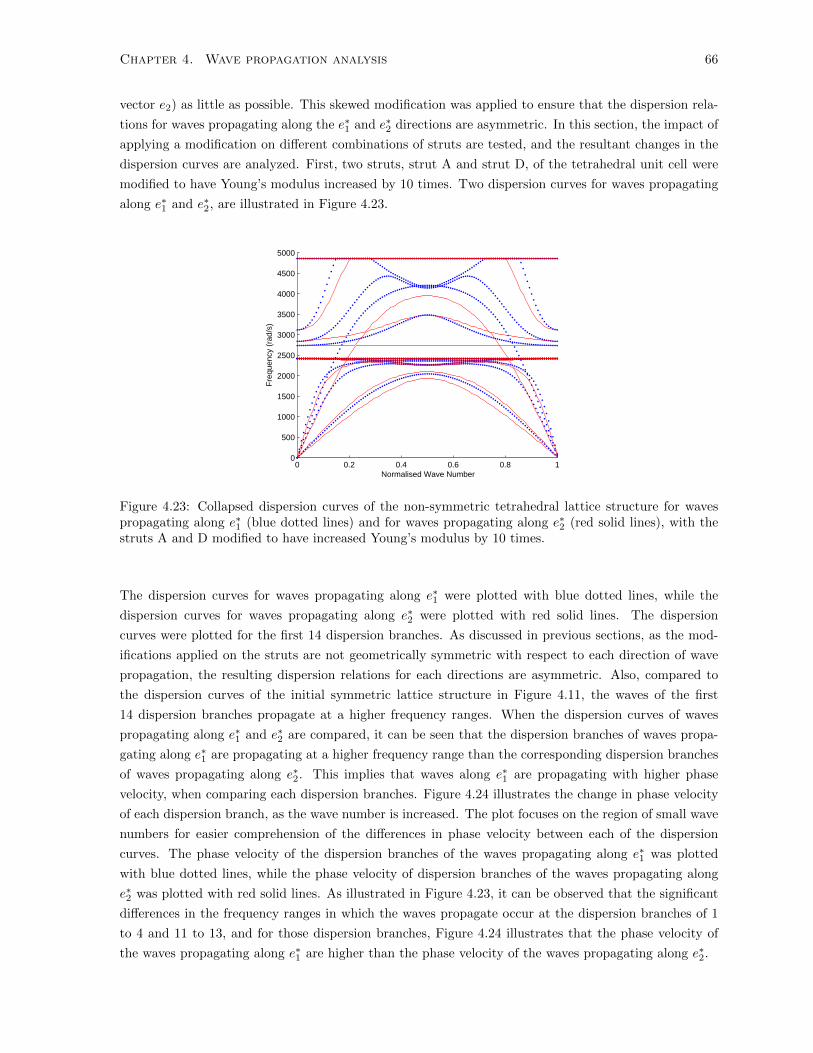
Chapter 4. Wave propagation analysis 66
vector e2) as little as possible. This skewed modification was applied to ensure that the dispersion rela-
tions for waves propagating along the e∗1 and e∗2 directions are asymmetric. In this section, the impact of
applying a modification on different combinations of struts are tested, and the resultant changes in the
dispersion curves are analyzed. First, two struts, strut A and strut D, of the tetrahedral unit cell were
modified to have Young’s modulus increased by 10 times. Two dispersion curves for waves propagating
along e∗1 and e∗2, are illustrated in Figure 4.23.
0 0.2 0.4 0.6 0.8 10
500
1000
1500
2000
2500
3000
3500
4000
4500
5000
Normalised Wave Number
Fre
quen
cy (
rad/
s)
Figure 4.23: Collapsed dispersion curves of the non-symmetric tetrahedral lattice structure for wavespropagating along e∗1 (blue dotted lines) and for waves propagating along e∗2 (red solid lines), with thestruts A and D modified to have increased Young’s modulus by 10 times.
The dispersion curves for waves propagating along e∗1 were plotted with blue dotted lines, while the
dispersion curves for waves propagating along e∗2 were plotted with red solid lines. The dispersion
curves were plotted for the first 14 dispersion branches. As discussed in previous sections, as the mod-
ifications applied on the struts are not geometrically symmetric with respect to each direction of wave
propagation, the resulting dispersion relations for each directions are asymmetric. Also, compared to
the dispersion curves of the initial symmetric lattice structure in Figure 4.11, the waves of the first
14 dispersion branches propagate at a higher frequency ranges. When the dispersion curves of waves
propagating along e∗1 and e∗2 are compared, it can be seen that the dispersion branches of waves propa-
gating along e∗1 are propagating at a higher frequency range than the corresponding dispersion branches
of waves propagating along e∗2. This implies that waves along e∗1 are propagating with higher phase
velocity, when comparing each dispersion branches. Figure 4.24 illustrates the change in phase velocity
of each dispersion branch, as the wave number is increased. The plot focuses on the region of small wave
numbers for easier comprehension of the differences in phase velocity between each of the dispersion
curves. The phase velocity of the dispersion branches of the waves propagating along e∗1 was plotted
with blue dotted lines, while the phase velocity of dispersion branches of the waves propagating along
e∗2 was plotted with red solid lines. As illustrated in Figure 4.23, it can be observed that the significant
differences in the frequency ranges in which the waves propagate occur at the dispersion branches of 1
to 4 and 11 to 13, and for those dispersion branches, Figure 4.24 illustrates that the phase velocity of
the waves propagating along e∗1 are higher than the phase velocity of the waves propagating along e∗2.

Chapter 4. Wave propagation analysis 67
0 0.05 0.1 0.15 0.2 0.250
50
100
150
Normalised Wave Number
Pha
se V
eloc
ity (
km/s
)
Figure 4.24: Phase velocity plot of the first 14 dispersion branches, focused on the small wave numbers.
Next, the dispersion curves were analyzed for different combinations of modified struts, while maintain-
ing the total number of modified struts to be unchanged. Here, two struts, strut A and strut F, of the
tetrahedral unit cell were modified to have Young’s modulus increased by 10 times. As the purpose of the
current section of the thesis is to observe the changes in dispersion curves when different combinations of
struts are modified, the dispersion curves for waves propagating along e∗1 of the current non-symmetric
lattice structure, in which strut A and F are modified, were compared with the dispersion curves for
waves propagating along e∗1 of the previous non-symmetric lattice structure, in which strut A and D
were modified (Figure 4.25). The dispersion curves of the current lattice structure were plotted with
blue dotted lines, while the dispersion curves of the previous lattice structure were plotted with red solid
lines.
0 0.2 0.4 0.6 0.8 10
500
1000
1500
2000
2500
3000
3500
4000
4500
5000
Normalised Wave Number
Fre
quen
cy (
rad/
s)
Figure 4.25: Comparisons of the dispersion curves for waves propagating along e∗1 when the struts Aand F were modified (blue dotted lines) and for waves propagating along e∗1 when the struts A and Dwere modified (red solid lines).

Chapter 4. Wave propagation analysis 68
Similarly, the dispersion curves for waves propagating along e∗2 of the current non-symmetric lattice
structure, in which struts A and F were modified, was compared with the dispersion curves for waves
propagating along e∗2 of the previous non-symmetric lattice structure, in which struts A and D were
modified (Figure 4.26). The dispersion curves of the current lattice structure were plotted with blue
dotted lines, while the dispersion curves of the previous lattice structure were plotted with red solid
lines.
0 0.2 0.4 0.6 0.8 10
500
1000
1500
2000
2500
3000
3500
4000
4500
5000
Normalised Wave Number
Fre
quen
cy (
rad/
s)
Figure 4.26: Comparisons of the dispersion curves for waves propagating along e∗2 when the struts Aand F were modified (blue dotted lines) and for waves propagating along e∗2 when the struts A and Dwere modified (red solid lines).
When comparing Figures 4.25 and 4.26, it can be seen that the frequency range, at which the waves
propagate, are unaffected, as for both cases waves propagate between 39.81 and 4859 rad/s. From Fig-
ure 4.23, it can be seen that the dispersion curves of waves propagating along e∗1 of the current lattice
structure have different band structure than the dispersion curves of waves propagating along e∗1 of the
previous lattice structure, but they show close resemblance to each other. There are, however, minor-
but-noticeable differences occurring at the dispersion branches of 1, 10, and 12, in which waves propagate
at different frequency ranges. Also, there exists no complete band gap for waves propagating along e∗1 for
both combinations of strut modifications. From Figure 4.24, the dispersion curves of waves propagating
along e∗2 of the current lattice structure have different band structure than the dispersion curves of waves
propagating along e∗2 of the previous lattice structure, but they show much significant differences in their
band structure. Due to the significant changes in the dispersion curves, when modifications are applied
on the different strut combinations, a complete band gap appears at the frequency range between 3751
and 4859 rad/s. The difference in magnitude of the change in band structure is related to the number
of nodes affected by the strut modifications that are connected to each boundary node of the lattice
structure, and how the changes in the nodes affect the global and reduced mass and stiffness matrices.
When the direction of the wave propagation is considered and the dispersion curves are plotted for
waves propagating along e∗1, the part of the global mass and stiffness matrices corresponding to the

Chapter 4. Wave propagation analysis 69
internal nodes connected to the boundary node e1 (node 1 of the tetrahedral lattice structure, which is
located at the end of strut A along the direction of the direct basis vector e1) and the boundary node
e1 itself are multiplied by a factor of ek1 , while the part of the matrices corresponding to the internal
nodes connected to the other boundary nodes and the other boundary nodes themselves are multiplied
by a factor of 1, since k2 and k3 are fixed at zero. As the wave number k1 increases, the values at
the part of the reduced mass and stiffness matrices corresponding to the internal nodes connected to
boundary node e1 and the boundary node e1 itself, would be changed as well, while the values at the
parts corresponding to the other internal nodes connected to other boundary nodes remain constant as
they are multiplied by 1. Therefore, for wave vectors propagating along the e∗1 direction, changes in the
values at the part of the global mass and stiffness matrices corresponding to the internal nodes that are
connected to the boundary node e1 would cause significant differences on the resulting eigen solution
for the same corresponding wave vectors. Knowing that the total number of internal nodes connected
to each boundary node are fixed for the same geometry of unit cell, the only factor that would cause
changes to the values at the parts of the global mass and stiffness matrices corresponding to the internal
nodes connected to the boundary node e1 is the changes in the design variables due to the modifications.
Therefore, when different combinations of modifications are considered for waves propagating along e∗1,
if the total number of internal nodes affected by the modifications, which are connected to the boundary
node e1, changes, then the differences in the dispersion curves and the band structures are likely to be
significant as there will be significant differences in the reduced mass and stiffness matrices. On the
other hand, considering that there are no changes in the number of internal nodes affected by modi-
fications and which are connected to the boundary node e1, the changes in the values at the parts of
the global mass and stiffness matrices corresponding to other internal nodes that are connected to the
other boundary nodes (the boundary nodes e2 and e3) would cause minor differences in the resulting
eigen solution for the same corresponding wave vectors, in which the minor differences occur from the
differences in the global mass and stiffness matrices.
Similarly, when the direction of the wave propagation is considered and the dispersion curves are mea-
sured for waves propagating along e∗2, the parts in the global mass and stiffness matrices corresponding
to the internal nodes connected to the boundary node e2 (node 2 of the tetrahedral lattice structure,
which is located at the end of strut B along the direction of direct basis vector e2) and the boundary node
e2 itself are multiplied by the factor of ek2 , while the parts of the matrices corresponding to the internal
nodes connected to the other boundary nodes and the other boundary nodes themselves are multiplied
by a factor of 1 (since k1 and k3 are fixed at zero). As the wave number k2 increases, the values at
the parts of the reduced mass and stiffness matrices corresponding to the internal nodes connected to
the boundary node e2 and the boundary node e2 itself would be changed as well, while the values at
the parts of the matrices corresponding to the other internal nodes connected to the other boundary
nodes remain constant as they are multiplied by 1. Therefore, for the wave vectors propagating along
the e∗2 direction, changes in the values at the parts of global mass and stiffness matrices corresponding
to the internal nodes that are connected to the boundary node e2 would cause significant differences in
the resulting eigen solution for the same corresponding wave vectors. Knowing that the total number
of internal nodes connected to each boundary node are fixed for the same geometry of unit cell, the
only factor that could cause changes in the values at the parts of the global mass and stiffness matrices
corresponding to the internal nodes connected to the boundary node e2, is the changes in the design

Chapter 4. Wave propagation analysis 70
variables due to the modification. Therefore, when different combinations of strut modifications are
considered for waves propagating along e∗2, if the total number of modified internal nodes connected
to the boundary node e2 changes, the differences in the dispersion curves and the band structures are
significant as there are significant differences in the reduced mass and stiffness matrices. On the other
hand, considering that there are no changes in the number of modified internal nodes connected to the
boundary node e2, changes in the values at the parts of the global mass and stiffness matrices corre-
sponding to the other internal nodes that are connected to the other boundary nodes (boundary nodes
e1 and e3) would cause minor differences on the resulting eigen solution for the same corresponding wave
vectors, in which the minor differences occur from the differences in the global mass and stiffness matrices.
In the above, when the modified struts were changed from struts A and D to struts A and F, the
total number of modified internal nodes connected to the boundary node e1 remained the same, while
the total number of modified internal nodes connected to the boundary node e2 changed. When the
dispersion curves of the waves propagating along e∗1 for each combination were compared, minor dif-
ferences could be seen in the band structure, although the band structures showed a close resemblance
to each other. On the other hand, when the dispersion curves of waves propagating along e∗2 for each
combination were compared, there were significant differences in the resulting band structures. The
above relation can be applied to other combinations of modifications, providing the same number of
struts are modified. Also, for different combinations of modifications, when the same number of struts
are modified, the frequency ranges at which the waves propagate in the dispersion curves do not change.
For all the different combinations of modifications, as long as only two struts are modified, the maximum
frequency range at which the waves propagate, at least for the first 14 dispersion branches, occurs at
4859 rad/s.
4.6.5 Impact of Increasing the Number of Struts Being Modified
In this section, the impact of increasing the number of struts being modified is analyzed. The modifica-
tions were applied to impact node 1, the boundary node located at the end of strut A, (along the direct
basis vector e1) as much as possible, while affecting node 2, the boundary node located at the end of strut
B, (along the direct basis vector e2) as little as possible. This skewed modification was applied to ensure
that the dispersion relations for the waves propagating along e∗1 and e∗2 were asymmetric. First, three
struts, namely strut A, C, and F, of the tetrahedral unit cell were modified to have Young’s modulus
increased by 10 times. As the purpose of the current section of the thesis is to observe the changes in the
dispersion curves when the number of modified struts are increased, the dispersion curves for the waves
propagating along the e∗1 directions of the current (three struts, A, C, and F, modified) non-symmetric
lattice structure are compared with the dispersion curves for the waves propagating along the e∗1 direc-
tions of the previous (two struts, A and F, modified) non-symmetric lattice structure. The dispersion
curves of the current lattice structure were plotted with blue dotted lines, while the dispersion curves of
the previous lattice structure (red solid line from Figure 4.25) were plotted with red solid lines.
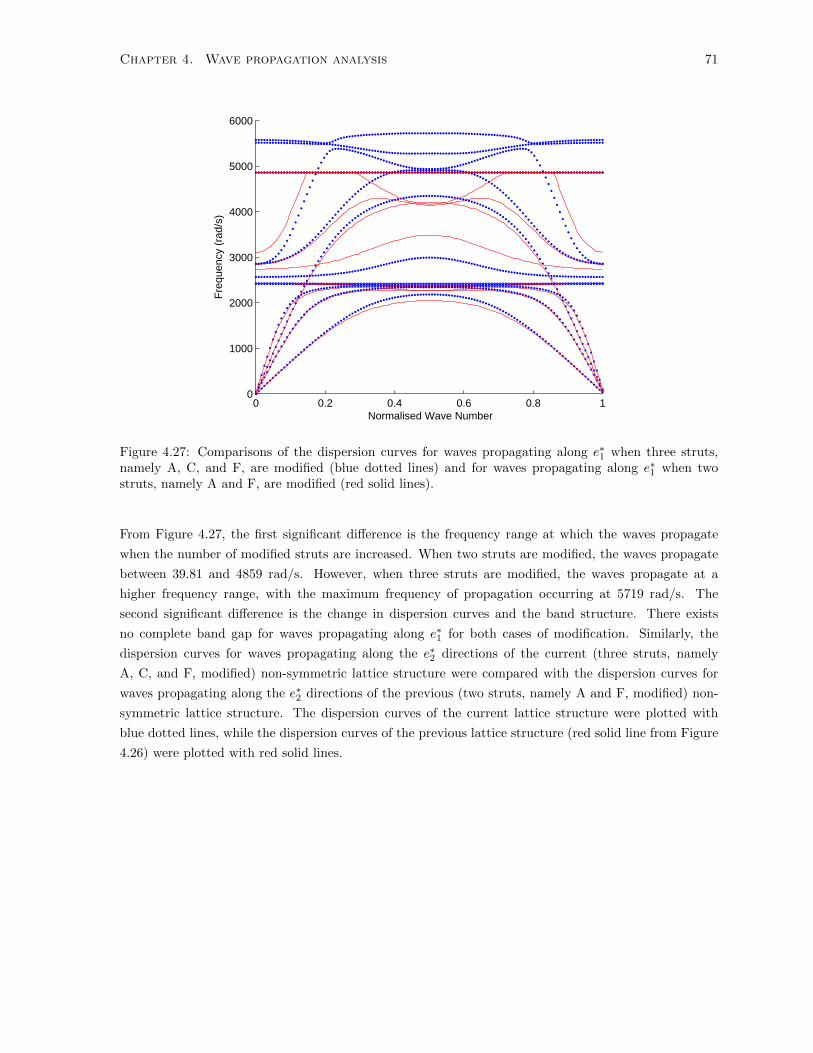
Chapter 4. Wave propagation analysis 71
0 0.2 0.4 0.6 0.8 10
1000
2000
3000
4000
5000
6000
Normalised Wave Number
Fre
quen
cy (
rad/
s)
Figure 4.27: Comparisons of the dispersion curves for waves propagating along e∗1 when three struts,namely A, C, and F, are modified (blue dotted lines) and for waves propagating along e∗1 when twostruts, namely A and F, are modified (red solid lines).
From Figure 4.27, the first significant difference is the frequency range at which the waves propagate
when the number of modified struts are increased. When two struts are modified, the waves propagate
between 39.81 and 4859 rad/s. However, when three struts are modified, the waves propagate at a
higher frequency range, with the maximum frequency of propagation occurring at 5719 rad/s. The
second significant difference is the change in dispersion curves and the band structure. There exists
no complete band gap for waves propagating along e∗1 for both cases of modification. Similarly, the
dispersion curves for waves propagating along the e∗2 directions of the current (three struts, namely
A, C, and F, modified) non-symmetric lattice structure were compared with the dispersion curves for
waves propagating along the e∗2 directions of the previous (two struts, namely A and F, modified) non-
symmetric lattice structure. The dispersion curves of the current lattice structure were plotted with
blue dotted lines, while the dispersion curves of the previous lattice structure (red solid line from Figure
4.26) were plotted with red solid lines.

Chapter 4. Wave propagation analysis 72
0 0.2 0.4 0.6 0.8 10
1000
2000
3000
4000
5000
6000
Normalised Wave Number
Fre
quen
cy (
rad/
s)
Figure 4.28: Comparisons of the dispersion curves for the waves propagating along e∗2 when three struts,namely A, C, and F, are modified (blue dotted lines) and for waves propagating along e∗2 when twostruts, namely A and F, are modified (red solid lines).
Similar to the phenomenon that occurs for the dispersion curves of waves propagating along e∗1, from
Figure 4.28, the first significant difference is the frequency range at which the waves propagate when the
number of modified struts are increased. When two struts are modified, the waves propagate between
39.81 and 4859 rad/s. However, when three struts are modified, the waves propagate at a higher
frequency range, with the maximum frequency of propagation occurring at 5715 rad/s. The second
significant difference is the change in dispersion curves and the band structure. There exist a complete
band gap at the frequency range of 3751-4859 rad/s, when two struts are modified; however, when three
struts are modified, a complete band gap occurs at the frequency range of 3279-4859 rad/s. The changes
in the dispersion curves and the ranges at which waves propagate occurs due to the change in the global
stiffness matrix. When an additional strut is modified to have Young’s modulus multiplied by 10, the
values of the parts of the global stiffness matrix corresponding to the nodes related to the modified struts
are all increased by a factor of 10 times too. Increasing the number of modified struts, increases the
parts of the global stiffness matrix at which the values are increased due to the modification. The same
phenomenon occurs when the number of modified struts are increased to four struts, such as struts A,
C, D, and F. Figure 4.29 illustrates the changes in the dispersion curves when the number of modified
struts are increased from three struts to four struts. The top figure compares the dispersion curves
for waves propagating along the e∗1 direction, while the bottom figure compares the dispersion curves
for waves propagating along the e∗2 direction. The dispersion curves of the lattice structure with four
modified struts are plotted with blue dotted lines, while the dispersion curves of the previous lattice
structure with three modified struts are plotted with red straight lines in this figure. Similar to the
phenomenon that occurs when the number of modified struts are increased from two to three, a different

Chapter 4. Wave propagation analysis 73
band structure of the dispersion curves are obtained, together with increased frequency ranges at which
the waves propagate. For waves propagating along e∗1, when three struts are modified, the maximum
frequency at which waves propagate occurs at 5719 rad/s. However, when four struts are modified, the
maximum frequency at which the waves propagate occurs at 6708 rad/s. Similarly, for waves propagating
along e∗2, when three struts are modified, the maximum frequency at which the waves propagate occurs
at 5715 rad/s. However, when four struts are modified, the maximum frequency at which the waves
propagate occurs at 6487 rad/s. There exists no complete band gap for waves propagating along e∗1 for
both cases of modification. For waves propagating along e∗2, there exists a complete band gap at the
frequency range of 3279 - 4859 rad/s, when three struts are modified. However, when four struts are
modified, there exists no band gap.
0 0.2 0.4 0.6 0.8 10
1000
2000
3000
4000
5000
6000
7000
Normalised Wave Number
Fre
quen
cy (
rad/
s)
0 0.2 0.4 0.6 0.8 10
1000
2000
3000
4000
5000
6000
7000
Normalised Wave Number
Fre
quen
cy (
rad/
s)
Figure 4.29: Comparisons of the dispersion curves for waves propagating along e∗1 when four, namelystruts A, C, D, and F, were modified (blue dotted lines, top) and for waves propagating along e∗1 whenthree struts, namely A, C, and F, were modified (red solid lines, top), and another comparison of thedispersion curves for waves propagating along e∗2 when four struts, namely A, C, D, and F, were modified(blue dotted lines, bottom) and for waves propagating along e∗2 when three struts, namely A, C, and F,were modified (red solid lines, bottom).

Chapter 4. Wave propagation analysis 74
A Further increase in the number of struts modified leads to the same phenomenon in the dispersion
curves. A different band structure is obtained, where the waves of each dispersion branch are propagating
at higher frequency ranges. When the number of modified struts is gradually increased, starting from
one strut being modified, the frequency range at which the waves propagate gradually increase toward
the frequency range at which waves propagate in a symmetric lattice structure (i.e. when all the struts
are modified). As the band structure changes as the number of modified struts increases, a new band
gap may be introduced in the new dispersion curves, or no band gap may exist for the new dispersion
curves. Combining these two behaviours, all band gaps, which are present for non-symmetric lattice
structures, always occur within the frequency ranges of the initial symmetric lattice structure (Figure
4.11) and the frequency ranges of the modified symmetric lattice structure (Figure 4.14).
4.6.6 Intuitive and Physical Understanding of the Dispersion Relations of a
Non-Symmetric Lattice Structure
In this chapter, the dispersion relations of symmetric and non-symmetric lattice structures have been
analyzed. In previous sections of this chapter, analyses of the dispersion curves of the symmetric and
non-symmetric lattice structures were performed primarily based on a mathematical perspective. In
this section, it is of interest to gain a physical understanding on the dispersion relations of the lattice
structures with various structural configurations.
Dispersion Relations of Symmetric Lattice Structure
First, in Section 4.6.2, the dispersion curves of the symmetric lattice structure, with all struts modified,
were analyzed. It was found that for symmetric lattice structures, an increase in the Young’s modulus
or a decrease in the density resulted in an increased frequency range at which the dispersion curves
occur. On the other hand, it was also found that a decrease in the Young’s modulus or a increase in
the density resulted in a decreased frequency range at which the dispersion curves occur. A physical
understanding of these results can be obtained by studying how waves propagate in different mediums.
Wave propagation through a medium, in another perspective, is the transfer of energy from one point of
the medium to another. If the medium is modified to have an increased Young’s modulus, the medium
becomes much stiffer and the atoms of the medium are then held more tightly to each other. As the
atoms are tightly held together, the waves propagate through the medium at a much faster speed, leading
the waves to propagate at a higher frequency. However, if the medium has a decreased Young’s modulus,
and therefore is less stiff, the atoms of the medium are held more widely apart from each other, which
causes the waves to propagate at a slower speed, leading them to propagate at a lower frequency range.
On the other hand, if the density of the medium is increased, the size and mass of the atoms of the
medium are increased. In order for waves to propagate through the heavier medium, more energy is
required. Hence, when the density of the medium is increased, the waves propagate at a lower frequency.
However, if the density of the medium is decreased, the size and mass of the atoms are decreased, thus
allowing the waves to be able to propagate much easier than before, and allowing the waves to propagate
at a higher frequency range.

Chapter 4. Wave propagation analysis 75
Dispersion Relations of Non-Symmetric Lattice Structure: Impact of Modifying Different
Combinations of Struts of the Lattice Structure
A second major analysis on the dispersion relations was made on the impact of applying modifications
on different combinations of struts of the non-symmetric lattice structure, which was covered in Section
4.6.4. In that section, it was analyzed that as long as the total number of struts being modified are
fixed, the dispersion curves of each of the different combinations of strut modification occur at the same
frequency ranges with each other, even though the band structures are different from each other. A
physical understanding of this dispersion relation can be obtained based on the analysis made above. If
struts A and B are modified to have differing Young’s modulus, in the context of the overall unit lattice
cell, the overall structure is as stiff as when other combinations of two struts are modified to have the
same differing Young’s modulus values. Hence, waves would propagate at a similar frequency through
the non-symmetric lattice structure, as long as same number of struts are modified to have increased
Young’s modulus values with the same modifications. Likewise, the frequency ranges at which the waves
propagate for the dispersion curves are similar for various non-symmetric lattice structures with any
combination of three struts being modified, while each of the dispersion curves would have a different
band structure.
Dispersion Relations of Non-Symmetric Lattice Structure: Impact of Increasing the Num-
ber of Struts Being Modified
In Section 4.6.5, the impact of increasing the number of modified struts was analyzed. Throughout
the analysis, it was found that gradually increasing the number of struts being modified, increases
the frequency range at which the dispersion curves occur. For instance, the frequency range at which
waves propagate when three struts are modified to have a higher Young’s modulus, occurs at a higher
frequency range than when only two struts are modified to have an increased Young’s modulus. Likewise,
the frequency range at which waves propagate when four struts are modified to have a higher Young’s
modulus, occurs at a higher frequency range than when three struts are modified to have an increased
Young’s modulus. As such, as more struts are modified for a non-symmetric lattice structure to gain an
increased Young’s modulus, the frequency range at which the waves propagate tends to occur at higher
frequency. The physical reasoning behind this phenomena is also related to the reasoning made above.
In the context of a unit lattice cell, if a greater number of struts are modified to have an increased
Young’s modulus, the overall lattice cell becomes stiffer. Hence, when waves are propagating through
the lattice unit cell, as the atoms of the unit cell are more stiff and held more tightly close to each
other, the waves will tend to propagate at a higher frequency. On the other hand, if more struts are
modified to have a reduced Young’s modulus, in the context of the overall unit cell, the unit cell is less
stiff and the atoms are spread further apart from each other. As a result, when more struts are modified
to have a decreased Young’s modulus, the waves would propagate at a lower frequency. Similarly, as the
number of struts being modified is increased, causing the structure to have an increased density for each
strut, in the context of the overall unit cell, it would require more energy for the waves to propagate
through, thereby causing waves to propagate at a lower frequency. Likewise, if the number of struts
being modified is gradually increased to have a lower density, the overall unit cell would have a lower
density, allowing the waves to propagate at a higher frequency.
Chapter 4. Wave propagation analysis 76
4.6.7 Significance of the Asymmetric Dispersion Relations
The strength of non-symmetric lattice structures with asymmetric dispersion relations comes from the
high flexibility they offer when designing and tailoring lattice structures and dispersion curves. First,
consider a structure with waves propagating in multiple directions. For applications of the lattice struc-
ture as a noise absorber, in which the waves are propagating in all directions within the system, the
symmetric dispersion relations are required to satisfy the need for a band gap to be present at the desired
frequency range, with a common band gap required for all waves propagating in all directions.
However, consider a system where waves are known to propagate in certain directions only, or a system
where only the waves propagating in certain directions are of interest, such as a system with guided waves
where waves are propagating in specific directions. A cylindrical water pipe is an example of a system
with guided waves. Within the cylindrical pipeline, the acoustic wave propagates in a direction along the
centerline of the pipe. If lattice structures are to be used for the applications with cylindrical pipeline,
symmetric dispersion relations give only one type of dispersion curve, which is applicable for waves prop-
agating in all directions. However, by breaking the symmetry and giving asymmetric dispersion relations,
many numbers of different dispersion curves with varying band structures can be generated, while it is
only required to satisfy waves propagating in a specific direction, which is along the centerline of the
cylindrical pipe. By increasing the number of struts being modified, more different choices of dispersion
curves are generated. Furthermore, by changing the different combinations of struts to be modified,
the possible dispersion curves to explore can be further increased. Therefore, while in symmetric dis-
persion relations, only single dispersion curves is provided to tailor around, the asymmetric relations
provide much more choices of dispersion curves to tailor around, therefore providing more ways to design
and optimize the lattice structure and its band gap. Also, asymmetric dispersion relations are easier
to tailor as the dispersion relations of the waves propagating along unnecessary directions can be ignored.
Second, consider a system with waves propagating in multiple directions, in which the different band
gaps are required for each of the waves propagating in each of the different directions. Achieving such
a goal with a symmetric lattice structure is difficult as the symmetric lattice structure results in one
symmetric dispersion curves. Hence, that one symmetric dispersion curve must have multiple band
gaps, each appearing at the different desired frequency ranges that satisfy the requirement for each wave
propagating in each of the different direction. However, if the dispersion relations are asymmetric, as
the dispersion relations are different for different directions of wave propagation, and as there are many
more different variations of asymmetric dispersion curves that can be studied, the asymmetric dispersion
relations provide higher flexibility for achieving that goal.
4.6.8 Impact of Changing the Other Design Variables
Changing the Young’s Modulus and the Density
In the previous sections, the thesis focused on the modification with the Young’s modulus value of
the struts being multiplied by 10. In this section, the impact of applying different modifications are
discussed, such as applying different values of the Young’s modulus or changed values of the density.

Chapter 4. Wave propagation analysis 77
For a symmetric lattice structure, in which all the struts are modified with the same changes in the
design variables, a change in the design variables of Young’s modulus or the density simply applies a
scaling effect to the dispersion curves while maintaining the same band structures. As discussed in Sec-
tion 4.6.2, when the Young’s modulus or the density of all the struts are modified, the dispersion curves
of the modified symmetric lattice structure is simply scaled by the factor of√
Eρ . Hence, increasing
the Young’s modulus or decreasing the density of all the struts simply increases the scale of the disper-
sion curves, whereby the waves of the modified symmetric lattice structure propagate at an increased
frequency range. On the other hand, decreasing the Young’s modulus or increasing the density of all
struts decreases the scale of the dispersion curves, whereby the waves of the modified symmetric lattice
structure propagate at a reduced frequency range.
For non-symmetric lattice structures, in which only one or more, but not all of the struts are modi-
fied, a change in the Young’s modulus or density no longer applies a scaling effect. As discussed in
Section 4.6.3, when only part of the unit lattice cell is modified, the expressions for the mass and stiff-
ness matrices are no longer related as a scalar factor. Hence, when Young’s modulus or the density
is changed as modifications for non-symmetric lattice structures, different dispersion curves and band
structures are obtained. For waves propagating in different directions of the non-symmetric lattice struc-
tures, the symmetric/asymmetric relations on the resulting dispersion curves are related to the location
at which the modifications are applied on the structure. Similar to the discussions in Section 4.6.3,
when the density of the struts are changed as a modification, if the modifications applied on the lattice
structure are geometrically symmetric with respect to each direction of wave propagation, symmetric
dispersion relations between waves propagating along each direction are obtained; whereas if the modifi-
cation applied on the lattice structure are not geometrically symmetric with respect to each direction of
wave propagation, asymmetric dispersion relations are present. Likewise, as illustrated in Section 4.6.4,
when different combinations of struts are modified to have changed values in density, different dispersion
curves are generated.
The differences in dispersion relations when different design variables are modified can be observed
when gradually increasing the number of struts modified. In Section 4.6.5, for the modifications with
an increased Young’s modulus, it was discussed that when the number of modified struts was gradually
increased, starting from one strut being modified, the frequency range at which the waves propagate
gradually increased toward the frequency range at which waves propagate in a symmetric lattice struc-
ture, i.e. a structure in which all the struts are modified. Based on the same relation, if Young’s modulus
of the modified struts is reduced instead, when the number of modified struts are gradually increased,
starting from one strut being modified, the frequency range at which the waves propagate gradually
decreases toward the frequency range at which waves propagate in a symmetric lattice structure. On
the other hand, increasing the density of the modified struts for a symmetric lattice structure causes the
dispersion curves to be scaled down by a factor of√
Eρ . Therefore, if the density is increased for the
modified struts of non-symmetric lattice structures, when the number of modified struts are gradually
increased, starting from one strut being modified, the frequency range at which the waves propagate will
gradually decrease. Likewise, if the density is decreased for the modified struts of non-symmetric lattice
structures, when the number of modified struts are gradually increased, starting from one strut being
modified, the frequency range at which the waves propagate will gradually increase. Another difference
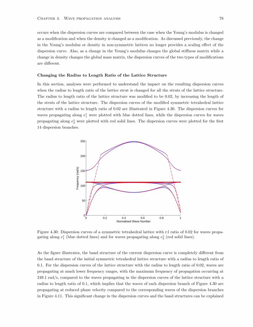
Chapter 4. Wave propagation analysis 78
occurs when the dispersion curves are compared between the case when the Young’s modulus is changed
as a modification and when the density is changed as a modification. As discussed previously, the change
in the Young’s modulus or density in non-symmetric lattices no longer provides a scaling effect of the
dispersion curve. Also, as a change in the Young’s modulus changes the global stiffness matrix while a
change in density changes the global mass matrix, the dispersion curves of the two types of modifications
are different.
Changing the Radius to Length Ratio of the Lattice Structure
In this section, analyses were performed to understand the impact on the resulting dispersion curves
when the radius to length ratio of the lattice strut is changed for all the struts of the lattice structure.
The radius to length ratio of the lattice structure was modified to be 0.02, by increasing the length of
the struts of the lattice structure. The dispersion curves of the modified symmetric tetrahedral lattice
structure with a radius to length ratio of 0.02 are illustrated in Figure 4.30. The dispersion curves for
waves propagating along e∗1 were plotted with blue dotted lines, while the dispersion curves for waves
propagating along e∗2 were plotted with red solid lines. The dispersion curves were plotted for the first
14 dispersion branches.
0 0.2 0.4 0.6 0.8 10
50
100
150
200
250
Normalised Wave Number
Fre
quen
cy (
rad/
s)
Figure 4.30: Dispersion curves of a symmetric tetrahedral lattice with r:l ratio of 0.02 for waves propa-gating along e∗1 (blue dotted lines) and for waves propagating along e∗2 (red solid lines).
As the figure illustrates, the band structure of the current dispersion curve is completely different from
the band structure of the initial symmetric tetrahedral lattice structure with a radius to length ratio of
0.1. For the dispersion curves of the lattice structure with the radius to length ratio of 0.02, waves are
propagating at much lower frequency ranges, with the maximum frequency of propagation occurring at
249.1 rad/s, compared to the waves propagating in the dispersion curves of the lattice structure with a
radius to length ratio of 0.1, which implies that the waves of each dispersion branch of Figure 4.30 are
propagating at reduced phase velocity compared to the corresponding waves of the dispersion branches
in Figure 4.11. This significant change in the dispersion curves and the band structures can be explained
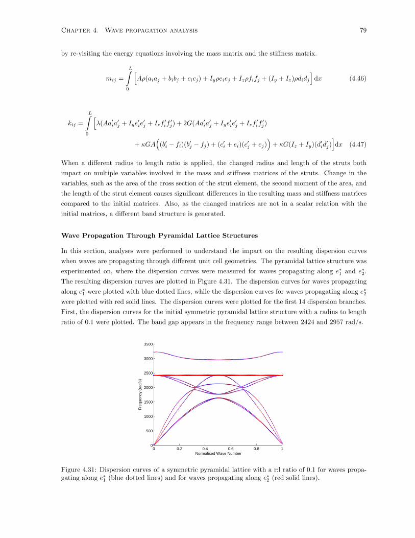
Chapter 4. Wave propagation analysis 79
by re-visiting the energy equations involving the mass matrix and the stiffness matrix.
mij =
L∫0
[Aρ(aiaj + bibj + cicj) + Iyρeiej + Izρfifj + (Iy + Iz)ρdidj
]dx (4.46)
kij =
L∫0
[λ(Aa′ia
′j + Iye
′ie′j + Izf
′if′j) + 2G(Aa′ia
′j + Iye
′ie′j + Izf
′if′j)
+ κGA(
(b′i − fi)(b′j − fj) + (c′i + ei)(c′j + ej)
)+ κG(Iz + Iy)(d′id
′j)]dx (4.47)
When a different radius to length ratio is applied, the changed radius and length of the struts both
impact on multiple variables involved in the mass and stiffness matrices of the struts. Change in the
variables, such as the area of the cross section of the strut element, the second moment of the area, and
the length of the strut element causes significant differences in the resulting mass and stiffness matrices
compared to the initial matrices. Also, as the changed matrices are not in a scalar relation with the
initial matrices, a different band structure is generated.
Wave Propagation Through Pyramidal Lattice Structures
In this section, analyses were performed to understand the impact on the resulting dispersion curves
when waves are propagating through different unit cell geometries. The pyramidal lattice structure was
experimented on, where the dispersion curves were measured for waves propagating along e∗1 and e∗2.
The resulting dispersion curves are plotted in Figure 4.31. The dispersion curves for waves propagating
along e∗1 were plotted with blue dotted lines, while the dispersion curves for waves propagating along e∗2
were plotted with red solid lines. The dispersion curves were plotted for the first 14 dispersion branches.
First, the dispersion curves for the initial symmetric pyramidal lattice structure with a radius to length
ratio of 0.1 were plotted. The band gap appears in the frequency range between 2424 and 2957 rad/s.
0 0.2 0.4 0.6 0.8 10
500
1000
1500
2000
2500
3000
3500
Normalised Wave Number
Fre
quen
cy (
rad/
s)
Figure 4.31: Dispersion curves of a symmetric pyramidal lattice with a r:l ratio of 0.1 for waves propa-gating along e∗1 (blue dotted lines) and for waves propagating along e∗2 (red solid lines).

Chapter 4. Wave propagation analysis 80
Next, the dispersion curves for a symmetric pyramidal lattice structure with a radius to length ratio of
0.02 were plotted for waves propagating along e∗1 and e∗2. The dispersion curves for waves propagating
along e∗1 were plotted with blue dotted lines, while the dispersion curves for waves propagating along e∗2
were plotted with red solid lines. The dispersion curves were plotted for the first 14 dispersion branches,
and it could be seen that there exists no complete band gap within the first 14 dispersion branches
(Figure 4.32).
0 0.2 0.4 0.6 0.8 10
50
100
150
200
250
Normalised Wave Number
Fre
quen
cy (
rad/
s)
Figure 4.32: Dispersion curves of a symmetric pyramidal lattice with a r:l ratio of 0.02 for wavespropagating along e∗1 (blue dotted lines) and for waves propagating along e∗2 (red solid lines).
When the wave propagation behaviour of the waves along e∗1 and e∗2 were analyzed, the resulting disper-
sion curves of the pyramidal lattice structures can be seen to be very similar to the dispersion curves
of the tetrahedral lattice structures. While the band structures illustrate minor insignificant differences
in small regions of the dispersion curves, the same behaviours, which were analyzed and discussed in
the previous sections for wave propagation in the tetrahedral lattice structures, were also observed for
the waves propagating in the pyramidal lattice structures. Hence, the analysis and discussions outlined
above for symmetric and non-symmetric tetrahedral lattice structures can also be applied for lattice
structures with different unit cell geometries.

Chapter 5
Conclusion and Future
Recommendations
5.1 Conclusion
Through the application of the finite element analysis, wave propagation behaviour through symmetric
and non-symmetric 3D lattice structures were analyzed. The analysis was performed on the lattice struc-
tures of two different geometries: tetrahedral and pyramidal lattice structures. The symmetric lattice
structure refers to a structure in which all struts of the lattice have the same design variables, while the
non-symmetric lattice structure refers to a structure in which the struts have modified design variables.
The eigenfrequencies to plot the dispersions curves were obtained by solving the eigenvalue problem,
with the input wave vectors limited to the waves propagating along the e∗1 and e∗2 directions, in order to
compare the dispersion relations of waves propagating along the e∗1 and e∗2 directions through symmetric
and non-symmetric lattice structures.
First, two symmetric lattice structures with a tetrahedral lattice structure were studied: initial sym-
metric lattice structure and a modified symmetric structure. When the Young’s modulus or density of
all the struts was changed, while the other design variables were fixed to stay the same, the resulting
dispersion curves were simply the scaled dispersion curves of the initial symmetric lattice structure by
a factor of√
Eρ . This was explained by analyzing how the design variables impact on the mass matrix
and the stiffness matrix of the eigenvalue problem. When only the Young’s modulus and/or density was
changed, the mass and stiffness matrices of the initial and modified symmetric lattice structures remained
constant, and were simply scaled based on the ratio of the changed values of the Young’s modulus and
density. Therefore, when the dispersion curve of the initial symmetric lattice structure were obtained,
the dispersion curves after the change in the Young’s modulus and/or density could be fully predicted.
However, this scalar relationship did not apply when other design variables, such as the radius or length
of the overall struts, were changed. The change in the other design variables impacted the mass matrix
and the stiffness matrix heavily. As the change in the other design variables led to entirely different mass
and stiffness matrices, the resulting dispersion curves were expected to provide different band structures.
Second, the non-symmetric lattice structures were studied. The effect of the change in design variables
81

Chapter 5. Conclusion and Future Recommendations 82
were analyzed when only one or more struts was modified rather than modifying the design variables for
all the struts. Unlike the behaviours in symmetric lattice structures, a change in the Young’s modulus
or density for non-symmetric lattice structures no longer performed as a tool for scaling the dispersion
curves, since the stiffness and mass matrices of the non-symmetric lattice structure could no longer be
expressed as the scalar factor of the initial symmetric lattice structure. Therefore, for non-symmetric
lattice structures, when any design variable is changed, new band structures of the dispersion curves can
be expected.
The analysis of the non-symmetric lattice structure with waves propagating along e∗1 and e∗2, showed
three distinct relations. First, when the modifications applied on the struts with respect to the waves
propagating along e∗1 direction, was applied on the struts at geometrically symmetric location with re-
spect to the waves propagating along e∗2 directions instead, the resulting dispersion relations between the
waves propagating along e∗1 and e∗2 were symmetric, in which the dispersion curves of waves propagating
along e∗1 and e∗2 of the same non-symmetric lattice structure were the same. On the other hand, if the
modifications applied on the struts are not geometrically symmetric with respect to each direction of
the wave propagation, the resulting dispersion relations between the waves propagating in each direc-
tion were asymmetric, in which the dispersion curves of waves propagating along e∗1 and e∗2 of the same
non-symmetric lattice structure were different. Second, when different combinations of modifications
were applied, the resulting dispersion curves showed a different band structure. When the total number
of struts being modified was kept constant, and only different combinations of struts were modified,
the frequency ranges at which waves propagated along e∗1 and e∗2 of the non-symmetric lattice structure
remained relatively close to each other. Third, starting from a non-symmetric lattice structure with only
one modified strut, when the number of modified struts was gradually increased, the resulting dispersion
curves showed a gradual change in the frequency ranges at which the waves propagated. When the
modification increased the Young’s modulus or decreased the density of the struts, as the number of
modified struts was gradually increased, the resulting dispersion curves showed a gradual increase in
the frequency ranges at which the waves propagated, in fact toward the frequency ranges at which the
waves would propagate through a symmetric lattice structure with all the struts modified. When the
modification decreased the Young’s modulus or increased the density of the struts, as the number of
modified struts was gradually increased, the resulting dispersion curves showed a gradual decrease in the
frequency ranges at which the waves propagated, in fact toward the frequency ranges at which waves
would propagate through a symmetric lattice structure with all the struts modified. Moreover, as the
band structure changes as the number of modified struts increases, a new band gap may be introduced
in the new dispersion curves, or no band gap may exist for the new dispersion curves. Combining these
two behaviours, all the band gaps present for non-symmetric lattice structures, always occur within the
frequency ranges of the initial (not-modified) symmetric lattice structure and in the frequency ranges of
modified symmetric lattice structures.
Concluding the analysis, for symmetric lattice structures, a change in the Young’s modulus or den-
sity performs as a powerful tool for scaling the dispersion curves and its band gap, whereby both the
location of the band gap and the resulting band structure of the dispersion curves are predictable. While
this scaling effect in symmetric lattice structures seem powerful for optimizing the size and location of
the band gap, limitations in the changes in the design variables could be expected due to the require-

Chapter 5. Conclusion and Future Recommendations 83
ments of the structural properties of the lattice structure. For example, in the application of the lattice
structure in aerospace industries, a structure with a high stiffness and low density would be preferred.
To achieve these ideal structural properties, the amount that the Young’s modulus or density that could
be modified is likely to be limited. For instance, when a structure has a band gap at a high frequency
range, and the band gap is required to be at a lower frequency range, the change in band gap location
can be performed by reducing the Young’s modulus or by increasing the density in a symmetric lattice
structure, but at the risk of turning the structural properties to be less than ideal. Another weakness
of the symmetric lattice structure comes from the total number of dispersion curves available per each
design of the lattice structure. The symmetric lattice structures yield one dispersion curve, which is
symmetric for waves propagating in different directions. Therefore, the number of dispersion curves
to tailor is highly limited for the symmetric lattice structures. On the other hand, the non-symmetric
lattice structures with asymmetric dispersion relations show strength in terms of its high flexibility when
designing and tailoring the lattice structures and the dispersion curves. The asymmetric dispersion re-
lations provide large numbers of different dispersion curves with varying band structures, in which each
dispersion curve is unique for each different direction of wave propagation. By increasing the number of
struts being modified, more unique choices of dispersion curves are generated. Furthermore, by applying
different combinations of struts to be modified, the possible dispersion curves to explore are further
increased. Therefore, the asymmetric relations provide a large number of dispersion curves to tailor
around, providing more options to design and optimize the lattice structure and its band gap. Also,
asymmetric dispersion relations demonstrate great strength in terms of their flexibility when tailoring
the dispersion curves, as the dispersion relations of the waves propagating along unnecessary directions
can be ignored.
5.2 Future Recommendations
5.2.1 Multi-Tetrahedral/Pyramidal Non-Symmetric Unit Cell
The present thesis has focused on the analysis of the lattice structure, in which the unit lattice cell was
limited to a single tetrahedral or pyramidal structure. However, clusters of tetrahedral or pyramidal
structures can be defined as the single unit cell by making the structure non-symmetric. Figure 5.1
illustrates a 3 × 3 × 3 pyramidal lattice structure as a single unit cell, where the unit cell is defined as
non-symmetric by having one of the pyramidal at the centre (in red), making it different to the other
remaining pyramidal structures. Differences between the two types of pyramidal structures can be made
by applying different design variables for each type of pyramidal structure, or by applying differences in
the structure geometry by adding additional supporting struts in the pyramidal structure, as illustrated
in Figure 5.2.
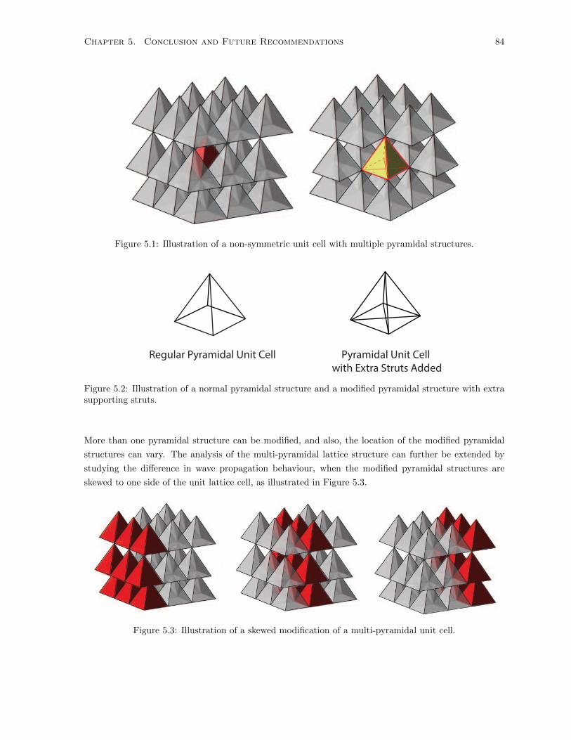
Chapter 5. Conclusion and Future Recommendations 84
Figure 5.1: Illustration of a non-symmetric unit cell with multiple pyramidal structures.
Regular Pyramidal Unit Cell Pyramidal Unit Cell
with Extra Struts Added
Figure 5.2: Illustration of a normal pyramidal structure and a modified pyramidal structure with extrasupporting struts.
More than one pyramidal structure can be modified, and also, the location of the modified pyramidal
structures can vary. The analysis of the multi-pyramidal lattice structure can further be extended by
studying the difference in wave propagation behaviour, when the modified pyramidal structures are
skewed to one side of the unit lattice cell, as illustrated in Figure 5.3.
Figure 5.3: Illustration of a skewed modification of a multi-pyramidal unit cell.

Chapter 5. Conclusion and Future Recommendations 85
5.2.2 Shape Shifting Lattice Structure
The introduction of the multi-tetrahedral or multi-pyramidal unit cell opens up the route to other
potential studies on the lattice structure, in which the lattice structure could handle two different band
gaps. First, a multi-tetrahedral lattice unit cell with four tetrahedral structures, in which the struts of
the tetrahedral structures have a radius to length ratio of 0.1, can be considered, as illustrated in Figure
5.4. The multi-tetrahedral unit cell can be turned into non-symmetric by applying a different material
for some struts. For example, in Figure 5.4, struts in orange colour are made out of polymer, while the
rest of the struts in light blue are made out of wax. If the structure goes through a procedure that could
melt and eliminate the struts made of wax completely without deforming or damaging the struts made
of polymer, the multi-tetrahedral unit cell becomes a unit cell with single tetrahedral structure with a
radius to length ratio of 0.05.
Figure 5.4: Illustration of a non-symmetric multi-tetrahedral unit cell (left), a non-symmetric multi-tetrahedral unit cell with two different materials (middle), and after the struts in one type of materialare eliminated (right).
Therefore, if there exists such a procedure that could eliminate struts made out of one type of material,
while not deforming the geometries or damaging the material properties of the strut made of the other
material, the unit cell of the lattice structure could change its shape through the procedure. Assuming
that a multi-tetrahedral unit cell would provide dispersion curves with unique band structure and band
gap phenomena, and that a tetrahedral unit cell with a radius to length ratio of 0.05 would provide a
different dispersion curves and band gap, the lattice structure could accommodate two different band
gaps in changing environment conditions.

Chapter 5. Conclusion and Future Recommendations 86
5.2.3 Lattice Structure as the Core of Sandwich Panel
The last potential future recommendation is the application of a lattice structure as the core of a sandwich
panel. In this thesis, the analysis was focused on the wave propagation behaviour through the lattice
structures. However, when lattice structures are applied as the core of a sandwich panel, the resulting
structure may provide different wave propagation behaviour due to the introduction of top and bottom
panels.
Figure 5.5: Illustration of a pyramidal lattice structure as the core of a sandwich panel.
Bibliography
[1] M. Arya and C.A. Steeves. Bandgaps in Octet Truss Lattices. Canadian Congress of Applied
Mechanics, 1 of 2:471–474, 2011.
[2] Manan Arya and Craig A Steeves. Wave Propagation in Three-Dimensional Periodic Lattices.
Technical report, 2011.
[3] A. Bazoune, Y.a. Khulief, and N.G. Stephen. Shape Functions of Three-Dimensional Timoshenko
Beam Element. Journal of Sound and Vibration, 259(2):473–480, January 2003.
[4] O. O. Bendiksen. Localization phenomena in structural dynamics. Chaos, solitons and fractals,
11:1621–1660, 2000.
[5] R.M. Christensen. Mechanics of cellular and other low-density materials. International Journal of
Solids and Structures, 37(1-2):93–104, 2000.
[6] John Chu. Topics in Designing Low Thermal Expansion Lattices at the Microscale. PhD thesis,
2011.
[7] Nastase-dan Ciobota. Standard Tessellation Language in Rapid Prototyping Technology. The
Science Bulletin of VALAHIA University, 7(7):81–85, 2012.
[8] V.S. Deshpande, N.A. Fleck, and M.F. Ashby. Effective properties of the octet-truss lattice material.
Journal of the Mechanics and Physics of Solids, 49:1747–1769, 2001.
[9] E. N. Economou and M. M. Sigalas. Classical wave propagation in periodic structures: Cermet
versus network topology. Physical Review B, 48(18):13434–13438, 1993.
[10] Henri P Gavin. Structural Element Stiffness, Mass, and Damping Matrices. Technical report, 2014.
[11] H Gleiter. Nanostructured Materials: Basic Concepts and Microstructure. Acta Materialia, 48:1–29,
2000.
[12] Dirk Hundertmark. A short introduction to Anderson localization. PhD thesis, 2007.
[13] R.G. Hutchinson and N.A. Fleck. The structural performance of the periodic truss. Journal of the
Mechanics and Physics of Solids, 54(4):756–782, April 2006.
[14] K.S Kumar, H Van Swygenhoven, and S Suresh. Mechanical behavior of nanocrystalline metals and
alloys. Acta Materialia, 51(19):5743–5774, November 2003.
87
Bibliography 88
[15] M.S. Kushwaha, P. Halevi, L Dobrzynski, and B Djafari-Rouhani. Theory of acoustic band structure
of periodic elastic composites. Physical review. B, Condensed matter, 49(4):2313–2322, January
1994.
[16] Yunhua Luo. An Efficient 3D Timoshenko Beam Element Homogeneous Euler-Lagrangian equations
governing 3D Timoshenko beam. 1(3):95–106, 2008.
[17] Giorgio Mantica. Wave propagation in almost-periodic structures, 1997.
[18] D.M. Mead. Wave Propagation in Continuous Periodic Structures: Research Contributions From
Southampton, 19641995. Journal of Sound and Vibration, 190(3):495–524, February 1996.
[19] M.A. Meyers, A. Mishra, and D.J. Benson. Mechanical properties of nanocrystalline materials.
Progress in Materials Science, 51(4):427–556, May 2006.
[20] Gisli Sigurbjorn Ottarsson. DYNAMIC MODELING AND VIBRATION ANALYSIS OF MIS-
TUNED BLADED DISKS Gısli Sigurbjorn Ottarsson. Technical report, 1994.
[21] J. Pearson. Solid State Physics, 2008.
[22] N.C. Perkins and C.D. Mote. Comments on curve veering in eigenvalue problems. Journal of Sound
and Vibration, 106(3):451–463, 1986.
[23] A. Srikantha Phani, J. Woodhouse, and N.A. Fleck. Wave propagation in two-dimensional periodic
lattices. The Journal of the Acoustical Society of America, 119(4):1995, 2006.
[24] Michel Piche Pierre R. Villeneuve. Photonic band gaps in two-dimensional square and hexagonal
lattices. The American Physical Society, 46(8):4969–4972, 1992.
[25] Yair Shapira. Solving PDEs in C ++. Technion-Israel Institute of Technology, 2006.
[26] Ole Sigmund and Jakob Søndergaard Jensen. Systematic design of phononic band-gap materials and
structures by topology optimization. Philosophical transactions. Series A, Mathematical, physical,
and engineering sciences, 361(1806):1001–1019, 2003.
[27] A. Vigliotti and D. Pasini. Stiffness and strength of tridimensional periodic lattices. Computer
Methods in Applied Mechanics and Engineering, 229-232:27–43, July 2012.
[28] N. Wicks and J.W. Hutchinson. Optimal truss plates. International Journal of Solids and Structures,
38(30-31):5165–5183, July 2001.
[29] C.H. Hodges Woodhouse and J. Vibration isolation from irregularity in a nearly periodic structure.
J. Accoust. Soc. AM, 74(September), 1983.
[30] E. N. Economou Zdetsis and A. Classical wave propagation in periodic structures. Rapid Commu-
nications, 40(2):3–8, 1989.