wave-equation migration velocity analysis. ii. subsalt...

Geophysical Prospecting, 2004, 52, 607–623

Wave-equation migration velocity analysis. II. Subsaltimaging examples

P. Sava∗ and B. BiondiDepartment of Geophysics, Stanford University, Mitchell Building, Stanford, CA 94305-2215, USA

Received February 2004, revision accepted July 2004

ABSTRACTSubsalt imaging is strongly dependent on the quality of the velocity model. How-ever, rugose salt bodies complicate wavefield propagation and lead to subsalt mul-tipathing, illumination gaps and shadow zones, which cannot be handled correctlyby conventional traveltime-based migration velocity analysis (MVA). We overcomethese limitations by the wave-equation MVA technique, introduced in a companionpaper, and demonstrate the methodology on a realistic synthetic data set simulatinga salt-dome environment and a Gulf of Mexico data set. We model subsalt propa-gation using wave paths created by one-way wavefield extrapolation. Those wavepaths are much more accurate and robust than broadband rays, since they inheritthe frequency dependence and multipathing of the underlying wavefield. We formu-late an objective function for optimization in the image space by relating an imageperturbation to a perturbation of the velocity model. The image perturbations aredefined using linearized prestack residual migration, thus ensuring stability, relativeto the first-order Born approximation assumptions. Synthetic and real data examplesdemonstrate that wave-equation MVA is an effective tool for subsalt velocity analysis,even when shadows and illumination gaps are present.

I N T R O D U C T I O N

Depth imaging of complex structures depends on the quality ofthe velocity model. However, conventional migration velocityanalysis (MVA) procedures often fail when the wavefield ex-hibits complex multipathing caused by strong lateral velocityvariations. Imaging under rugged salt bodies is an importantcase when ray-based MVA methods are not reliable. Sava andBiondi (2004) have presented the theory and the methodol-ogy of an MVA procedure based on wavefield extrapolationwith the potential of overcoming the limitations of ray-basedMVA methods. In this paper, we present the application of theproposed procedure to Sigsbee 2A, a realistic and challenging2D synthetic data set created by the SMAART JV (Paffenholz

Paper presented at the EAGE/SEG Summer Research Workshop,Trieste, Italy, August/September 2003.∗E-mail: [email protected]

et al. 2002) and to a 2D line extracted from a 3D real data setfrom the Gulf of Mexico.

Many factors determine the failure of ray-based MVA in asubsalt environment. Some of them are successfully addressedby our wave-equation MVA (WEMVA) method, whereas oth-ers, for example the problems that are caused by essentiallimitations of the recorded reflection data, are only partiallysolved by WEMVA.

An important practical difficulty encountered when usingrays to estimate velocity below rugose salt bodies is the insta-bility of ray tracing. Rough salt topology creates poorly illu-minated areas, or even shadow zones, in the subsalt region.The spatial distribution of these poorly illuminated areas isvery sensitive to the velocity function. Therefore, it is oftenextremely difficult to trace rays connecting a given point inthe poorly illuminated areas with a given point at the surface(two-point ray tracing). Wavefield extrapolation methods arerobust with respect to shadow zones and they always providewave paths suitable for velocity inversion.

C© 2004 European Association of Geoscientists & Engineers 607

608 P. Sava and B. Biondi

A related and more fundamental problem with ray-basedMVA is that rays poorly approximate actual wave paths whena band-limited seismic wave propagates through a rugose topof the salt. Figure 1 illustrates this issue by showing three band-limited (1–26 Hz) wave paths, also known in the literature asfat rays or sensitivity kernels (Woodward 1992; Pratt 1999;Dahlen, Hung and Nolet 2000). Each of these three wave pathsis associated with the same point source located at the surface,but corresponds to a different subsalt ‘event’. The top panelin Fig. 1 shows a wave path that could reasonably be approxi-mated using the method introduced by Lomax (1994) to tracefat rays using asymptotic methods. In contrast, the wave pathsshown in both the middle and bottom panels in Fig. 1 cannotbe well approximated using Lomax’s method. The amplitudeand shapes of these wave paths are significantly more com-plex than a simple fattening of a geometrical ray could everdescribe. The bottom panel illustrates the worst-case-scenariosituation for ray-based tomography because the variability ofthe top salt topology is on the same scale as the spatial wave-length of the seismic wave. The fundamental reason why truewave paths cannot be approximated using fattened geometri-cal rays is that they are frequency dependent. Figure 2 illus-trates this dependence by depicting the wave path shown inthe bottom panel of Fig. 1 as a function of the temporal band-width: 1–5 Hz (top), 1–16 Hz (middle) and 1–64 Hz (bottom).The width of the wave path decreases as the frequency band-width increases, and the focusing/defocusing of energy varieswith the frequency bandwidth.

The limited and uneven ‘illumination’ of both the reflec-tivity model and the velocity model in the subsalt region is achallenging problem for both WEMVA and conventional ray-based MVA (see Fig. 7 for an example of this problem). For thereflectors under salt, the angular bandwidth is drastically re-duced in the angle-domain common-image gathers (ADCIGs).This phenomenon is due to a lack of oblique wave paths in thesubsalt, causing a reduction in the ‘sampling’ of the velocityvariations in the subsalt. Consequently, the velocity inversionis more poorly constrained in the subsalt sediments than in thesediments on the side of the salt body.

Uneven illumination of subsalt reflectors is even more of achallenge than reduced angular coverage. It makes the veloc-ity information present in the ADCIGs less reliable by causingdiscontinuities in the reflection events and creating artefacts.MVA methods assume that when the migration velocity is cor-rect, events are flat in ADCIGs along the aperture-angle axis.Velocity updates are estimated by minimizing the curvatureof events in ADCIGs. MVA methods may provide biased es-timates where uneven illumination creates events that bend

along the aperture-angle axis, even where the image is createdwith the correct velocity. We address this issue by weightingthe image perturbations before inverting them into velocityperturbations. Our weights are functions of the ‘reliability’ ofthe moveout measurements in the ADCIGs.

WAV E - E Q U AT I O N M VA A L G O R I T H M

In this section, we briefly summarize the theory of wave-equation migration velocity analysis (WEMVA). In contrastwith the companion paper (Sava and Biondi 2004), we avoidmathematical detail and concentrate on the principles onwhich WEMVA is developed. Therefore, this section comple-ments the theory presented in Sava and Biondi (2004), and isdesigned as a quick introduction to WEMVA for the readerless interested in mathematical detail.

The computation of the velocity updates from the resultsof migrating the data with the current (background) velocitymodel comprises three main components that are summarizedby the flow chart in Fig. 3. The three components are labelledA, B and C on the chart. Box A corresponds to the computationof the background wavefield, based on the surface data andbackground slowness. Boxes B and C correspond respectivelyto the forward and adjoint WEMVA operator.

Using wavefield extrapolation, the data recorded at the sur-face (D) are downward continued to all depth levels, usingthe background slowness (S) to generate a background wave-field (U). The known background slowness (S) can incorpo-rate lateral variations. Extrapolation can be carried out withkernels corresponding to such methods as Fourier finite dif-ference (Ristow and Ruhl 1994), or generalized screen propa-gator (Rousseau, Calandra and de Hoop 2003). From the ex-trapolated wavefield, we can construct the background image(R) by applying a standard imaging condition, for example, asimple summation over frequencies.

The background wavefield (U) is an important componentof the WEMVA operator. This wavefield plays a role anal-ogous to the one played in traveltime tomography by theray-field obtained by ray tracing in the background model.The wavefield is the carrier of information and defines thewave paths along which we spread the velocity errors mea-sured from the migrated images obtained using the back-ground slowness function. The wavefield is band-limited, un-like a ray-field, which describes propagation of waves withan infinite frequency band. Therefore, the background wave-field provides a more accurate description of wave propaga-tion through complex media than the corresponding ray-field(Figs 1 and 2). Typical examples are salt bodies characterized

C© 2004 European Association of Geoscientists & Engineers, Geophysical Prospecting, 52, 607–623

Wave-equation migration velocity analysis II 609

Figure 1 Wave paths for frequencies between 1 and 26 Hz for various locations in the image and a point on the surface. Each panel is an overlayof three elements: the slowness model, the wavefield corresponding to a point source on the surface at x = 16 km, and wave paths from a pointin the subsurface to the source.



Figure 2 Frequency dependence of wave paths between a location in the image and a point on the surface. Each panel is an overlay of threeelements: the slowness model, the wavefield corresponding to a point source on the surface at x = 16 km, and wave paths from a point in thesubsurface to the source. The different wave paths correspond to frequency bands of 1–5 Hz (top), 1–16 Hz (middle) and 1–64 Hz (bottom).The larger the frequency band, the narrower the wave path. The end member for an infinitely wide frequency band corresponds to an infinitelythin geometrical ray.



dR

S

U

D

R

dW

dU

dSdS’

dW’

dU’

ADJOINToperator

FORWARDoperator

A

BC

imaging

imag

ing

extr

apol

atio

nsc

atte

ring

extr

apol

atio

n

Figure 3 WEMVA flow chart. Box A:the data recorded at the surface (D) areextrapolated in depth using the back-ground slowness (S) to generate thebackground wavefield (U); we transformthe background wavefield (U) into thebackground image (R) using an imagingoperator. Box B: the background wavefield(U) interacts with a slowness perturbation(dS) generating a scattered wavefield (dW);after depth extrapolation, we accumulatethe scattered wavefield into a wavefield per-turbation (dU); we transform the wavefieldperturbation (dU) into an image perturba-tion (dR) using an imaging operator. Box C:we transform the image perturbation (dR)into a wavefield perturbation (dU’) using theadjoint of the imaging operator; we upwardcontinue the adjoint wavefield perturbation(dU’) and, at every depth level, we isolate anadjoint scattered wavefield (dW’); using thebackground wavefield (U), we transform theadjoint scattered wavefield into an adjointslowness perturbation (dS’).

by large velocity contrasts where ray tracing is both unstableand inaccurate.

When evaluating the forward operator (Box B), the back-ground wavefield (U) interacts with a slowness perturbation(dS) and generates a scattered wavefield (dW) at every depthlevel. In our method, scattering is based on the first-order Bornapproximation, which assumes perturbations to be small inboth size and magnitude. This approximation is appropri-ate, because scattering occurs independently at every depthlevel. The contribution to the scattered wavefield is addedat each depth level, and the total scattered wavefield (dU)is extrapolated to depth, using the same numerical propaga-tor as the one used to extrapolate the background wavefieldfrom the surface data. Therefore, the wavefield perturbationat any depth level contains the accumulated effects of scat-tering and extrapolation from all the levels above it. Finally,we apply an imaging condition to the wavefield perturba-tion (dU) and obtain an image perturbation (dR) correspond-

ing to the slowness perturbation (dS) and the backgroundwavefield (U).

In migration velocity analysis, we are interested in the in-verse process, where we take an image perturbation (dR) andconstruct a slowness perturbation (dS). We obtain image per-turbations via image enhancement operators (residual move-out, residual migration, etc.) applied to the background im-age (R). Since the scattering operator is based on the Bornapproximation, we need to take special precautions to avoidcycle-skipping of the phase function. We overcome the Bornapproximation limitations by using linearized image pertur-bations, as described by Sava and Biondi (2004).

To invert the linearized image perturbation into slownessupdates by an iterative algorithm, such as the conjugate gra-dient (Golub and Loan 1983), we need to evaluate the adjointWEMVA operator (Box C) as well as the forward operator.From the image perturbation (dR), we construct an adjointwavefield perturbation (dU) by applying the adjoint imaging



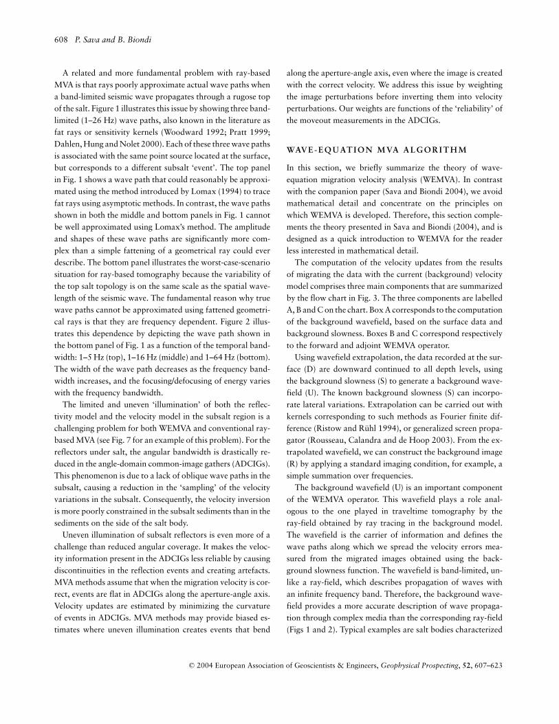
Figure 4 Monochromatic WEMVA example: (a) background wavefield; (b) slowness perturbation; (c) wavefield perturbation; (d) slownessbackprojection.

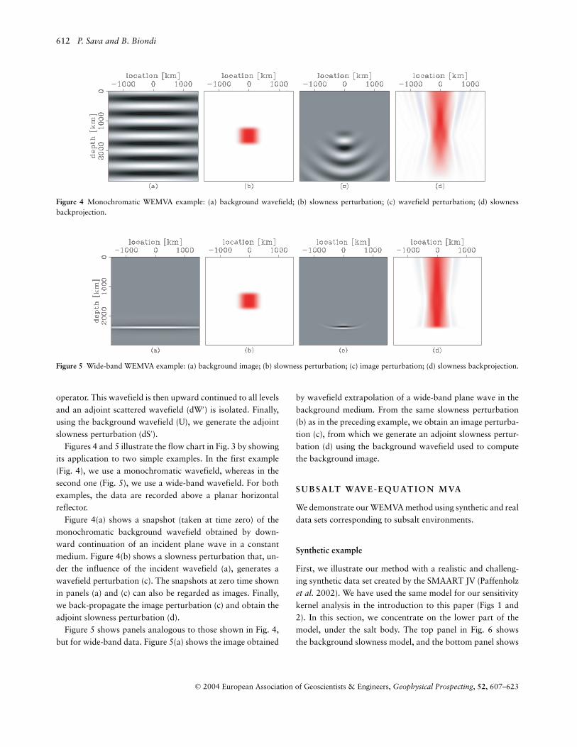
Figure 5 Wide-band WEMVA example: (a) background image; (b) slowness perturbation; (c) image perturbation; (d) slowness backprojection.

operator. This wavefield is then upward continued to all levelsand an adjoint scattered wavefield (dW′) is isolated. Finally,using the background wavefield (U), we generate the adjointslowness perturbation (dS′).

Figures 4 and 5 illustrate the flow chart in Fig. 3 by showingits application to two simple examples. In the first example(Fig. 4), we use a monochromatic wavefield, whereas in thesecond one (Fig. 5), we use a wide-band wavefield. For bothexamples, the data are recorded above a planar horizontalreflector.

Figure 4(a) shows a snapshot (taken at time zero) of themonochromatic background wavefield obtained by down-ward continuation of an incident plane wave in a constantmedium. Figure 4(b) shows a slowness perturbation that, un-der the influence of the incident wavefield (a), generates awavefield perturbation (c). The snapshots at zero time shownin panels (a) and (c) can also be regarded as images. Finally,we back-propagate the image perturbation (c) and obtain theadjoint slowness perturbation (d).

Figure 5 shows panels analogous to those shown in Fig. 4,but for wide-band data. Figure 5(a) shows the image obtained

by wavefield extrapolation of a wide-band plane wave in thebackground medium. From the same slowness perturbation(b) as in the preceding example, we obtain an image perturba-tion (c), from which we generate an adjoint slowness pertur-bation (d) using the background wavefield used to computethe background image.

S U B S A LT WAV E - E Q U AT I O N M VA

We demonstrate our WEMVA method using synthetic and realdata sets corresponding to subsalt environments.

Synthetic example

First, we illustrate our method with a realistic and challeng-ing synthetic data set created by the SMAART JV (Paffenholzet al. 2002). We have used the same model for our sensitivitykernel analysis in the introduction to this paper (Figs 1 and2). In this section, we concentrate on the lower part of themodel, under the salt body. The top panel in Fig. 6 showsthe background slowness model, and the bottom panel shows



Figure 6 Sigsbee 2A synthetic model: the background slowness model (top) and the correct slowness perturbation (bottom).

the slowness perturbation of the background model relative tothe correct slowness. Thus, we simulate a common subsalt ve-locity analysis situation where the shape of the salt is known,but the smoothly varying slowness subsalt is not fully known.Throughout this example, we denote horizontal location by x

and depth by z.The original data set was computed with a typical ma-

rine off-end recording geometry. Preliminary studies of thedata demonstrated that in some areas the complex over-burden causes events to be reflected with a negative reflec-tion angle (i.e. the source and receiver wave paths cross be-fore reaching the reflector). To avoid losing these events, weapplied the reciprocity principle and created a split-spreaddata set from the original off-end data set. This modifi-cation of the data set enabled us to compute symmetricADCIGs that are easier to analyse visually than the typicalone-sided ADCIGs obtained from marine data. Therefore, wedisplay the symmetric ADCIGs in Fig. 9 and Figs 13–15 . Dou-bling the data set also doubles the computational cost of ourprocess.

Figure 7 shows the migrated image using the correct slow-ness model. The top panel shows the zero offset of the prestackmigrated image, and the bottom panel depicts ADCIGs atequally spaced locations in the image. Each ADCIG corre-sponds roughly to the location directly above it.

This image highlights several characteristics of this modelthat make it a challenge for migration velocity analysis. Mostof the characteristics are related to the complicated wave pathsin the subsurface under rough salt bodies. Firstly, the angularcoverage under salt (x > 11 km) is much smaller than in thesedimentary section uncovered by salt (x < 11 km). Secondly,the subsalt region is marked by many illumination gaps orshadow zones, the most striking ones being located at x = 12and x = 19 km. The main consequence is that velocity analysisin the poorly illuminated areas is much less constrained thanin the well-illuminated zones, as will become apparent lateron in our example.

We begin by migrating the data with the background slow-ness (Fig. 8). As before, the top panel shows the zero offset ofthe prestack migrated image, and the bottom panel depicts



Figure 7 Migration with the correct slowness, using the Sigsbee 2A synthetic model. The zero offset of the prestack migrated image (top) andangle-domain common-image gathers at equally spaced locations in the image (bottom) are shown. Each ADCIG corresponds roughly to thelocation directly above it.

Figure 8 Migration with the background slowness, using the Sigsbee 2A synthetic model. The zero offset of the prestack migrated image (top)and angle-domain common-image gathers at equally spaced locations in the image (bottom) are shown. Each ADCIG corresponds roughly tothe location directly above it.



Figure 9 Residual migration for a common-image gather at x = 10 km, using the Sigsbee 2A synthetic model. The top panel depicts angle-domaincommon-image gathers for all values of the velocity ratio, and the bottom panel depicts the semblance panels used for picking. All gathers arestretched to eliminate the vertical movement corresponding to different migration velocities. The superimposed line indicates the picked valuesat all depths.

Figure 10 Sigsbee 2A synthetic model. The top panel depicts the velocity ratio difference �ρ = 1 − ρ at all locations; the bottom panel depictsa weight indicating the reliability of the picked values at every location. The picks in the shadow zone around x = 12 km are less reliable thanthe picks in the sedimentary region around x = 8 km. All picks inside the salt are disregarded.



Figure 11 Sigsbee 2A synthetic model: the correct slowness perturbation (top) and the inverted slowness perturbation (bottom).

angle-domain common-image gathers at equally spaced loca-tions in the image. Since the migration velocity is incorrect,the image is defocused and the angle gathers show significantmoveout. Furthermore, the diffractors at depths z = 7.5 kmand the fault at x = 15 km are defocused.

As described by Sava and Biondi (2004), we run prestackStolt residual migration for various values of a velocity ratioparameter ρ between 0.9 and 1.6, thus ensuring that a fairlywide range of the velocity space is spanned. Although residualmigration operates on the entire image globally, for displaypurposes we extract one gather at x = 10 km. Figure 9 (top)shows the ADCIGs for all velocity ratios and Fig. 9 (bottom)shows the semblance panels computed from the ADCIGs. Wepick the maximum semblance at all locations and all depths(Fig. 10), together with an estimate of the reliability of everypicked value which we use as a weighting function on the dataresiduals during inversion.

Based on the picked velocity ratio, we compute the lin-earized differential image perturbation, as described in the pre-ceding sections. Next, we invert for the slowness perturbation

depicted in the bottom panel of Fig. 11. For comparison, thetop panel of Fig. 11 shows the correct slowness perturbationrelative to the correct slowness. We can clearly see the effects ofdifferent angular coverage in the subsurface: at x < 11 km, theinverted slowness perturbation is better constrained verticallythan it is at x > 11 km.

Finally, we update the slowness model and remigrate thedata (Fig. 12). As before, the top panel shows the zero offsetof the prestack migrated image and the bottom panel showsangle-domain common-image gathers at equally spaced loca-tions in the image. With this updated velocity, the reflectorshave been repositioned to their correct location, the diffrac-tors at z = 7.5 km are focused and the ADCIGs are flatter thanin the background image, indicating that our slowness updatehas improved the quality of the migrated image.

Figures 13–15 show a more detailed analysis of the re-sults of our inversion, displayed as ADCIGs at various lo-cations in the image. In each figure, the panels correspondto migration with the correct slowness (left), the backgroundslowness (centre) and the updated slowness (right). Figure 13



Figure 12 Migration with the updated slowness, using the Sigsbee 2A synthetic model. The zero offset of the prestack migrated image (top) andangle-domain common-image gathers at equally spaced locations in the image (bottom) are shown. Each ADCIG corresponds roughly to thelocation directly above it.

corresponds to an ADCIG at x = 8 km, in the regionwhich is well illuminated. The angle gathers are clean, withclearly identifiable moveouts that are corrected after inversion.Figure 14 corresponds to an ADCIG at x = 10 km, in the re-gion with illumination gaps, clearly visible on the strong re-flector at z = 9 km at a scattering angle of about 20◦. Thegaps are preserved in the ADCIG from the image migratedwith the background slowness, but the moveouts are still easyto identify and correct. Finally, Figure 15 corresponds to anADCIG at x = 12 km, in a region which is poorly illuminated.In this case, the ADCIG is much noisier and the moveouts areharder to identify and measure. This region also correspondsto the lowest reliability, as indicated by the low weight of thepicks (Fig. 10). The gathers in this region contribute less tothe inversion and the resulting slowness perturbation is mainlycontrolled by regularization. Despite the noisier gathers, afterslowness update and remigration we recover an image reason-ably similar to the one obtained by migration with the correctslowness.

A simple visual comparison of the middle panels with theright and left panels in Figs 13–15 unequivocally demonstratesthat our WEMVA method overcomes the limitations related tothe linearization of the wave equation by using the first-orderBorn approximation. The images obtained using the initial ve-locity model (middle panels) are shifted vertically by severalwavelengths with respect to the images obtained using the truevelocity (left panels) and the estimated velocity (right panels).If the Born approximation were a limiting factor for the mag-nitude and spatial extent of the velocity errors that could beestimated with our WEMVA method, we would have been un-able to estimate a velocity perturbation sufficient to improvethe ADCIGs from the middle panels to the right panels.

Field data example

Our second example concerns a 2D line extracted from a3D subsalt data set from the Gulf of Mexico. We follow thesame methodology as that used for the preceding synthetic



Figure 13 Angle-domain common-image gathers at x = 8 km using the Sigsbee 2A synthetic model. Each panel corresponds to a differentmigration velocity: migration with the correct velocity (left), migration with the background velocity (centre) and migration with the updatedvelocity (right).

Figure 14 As Fig. 13, at x = 10 km.



Figure 15 As Fig. 13, at x = 12 km.

example. In this case, however, we run several non-linear it-erations of WEMVA, each involving wavefield linearization,residual migration and inversion.

Figure 16 (top) shows the image migrated with the back-ground velocity superimposed on the background slowness.This image serves as a reference against which we check theresults of our velocity analysis. Two regions of interest arelabelled A and B in the figure. The right edge of the modelcorresponds to a salt body. The top edge of the image is notat the surface, because we have datumed the surface data to adepth below the well-imaged overhanging salt body.

As for the preceding example, we run residual migrationand analyse the moveouts of ADCIGs. Figure 17 shows thisanalysis at one location in the left part of the model. The leftpanel shows this ADCIG changing according to the velocityratio parameter, while the right panel shows the semblancescan corresponding to each of these ratios. The superimposedline is a pick of maximum semblance, indicating the flattestADCIG at every depth level. This analysis is repeated at ev-ery location, from which we obtain two maps: a map of the

residual migration parameter at every location in the image(Fig. 16, middle) and a map of the weight indicating the reli-ability of the picks (Fig. 16, bottom). The residual migrationparameter is plotted relative to 1 (indicated in white), thereforethe whiter the map, the flatter the ADCIGs. The stack of thebackground images is superimposed for visual identificationof image features. Next, we generate an image perturbationbased on the residual migration picks in Fig. 16 (middle) andinvert for slowness perturbation using the weights in Fig. 16(bottom) as an approximation for the inverse data covariancematrix.

The results obtained after two non-linear iterations ofWEMVA are shown in Figs 18 and 19. As for Fig. 16, thethree panels show the migrated image superimposed on slow-ness (top), residual migration picks (middle) and pick weights(bottom). Two regions in which changes occur are labelled Aand B.

For both iterations 1 and 2, the residual migration picksconverge towards 1, indicating flatter ADCIGs, therefore bet-ter focused images. Reflectors in both regions shift vertically,



Figure 16 Gulf of Mexico data. Migratedimage superimposed on slowness (top),residual migration picks (middle) and pick-ing weight (bottom). The migration corre-sponds to the background slowness.

according to the slowness changes. A noteworthy feature is theimproved continuity of the strongest reflectors in the regionlabelled B.

Both images improve after migration with the updated slow-nesses from WEMVA. However, there are regions where theimage changes are small, if present at all. For example, theregion to the left of ‘B’, which corresponds to a shadow zonecaused by the salt structure in the upper part of the model,does not change. Better velocity estimates could be made inthis region with 3D data, since the shadow zones have three-dimensional expressions.

C O N C L U S I O N S

Subsalt imaging is one of the most challenging problems ofmodern seismic imaging because the sharp and irregular salt–

sediment interface causes multipathing and uneven illumi-nation. Wavefield-continuation migration methods producehigh-quality images under salt, but the estimation of the migra-tion velocity function in the subsalt is an unresolved problem.Conventional MVA methods based on traveltimes computedby ray tracing often fail to provide reliable velocity estimatesbecause ray tracing is unstable and sensitive to the fine detailsof the salt–sediment interface.

We have demonstrated that the wave-equation migrationvelocity analysis (WEMVA) method (Sava and Biondi 2004)overcomes many of the problems encountered by ray-basedMVA methods when estimating velocity under salt. We used acomplex and a realistic subsalt data set to test our methodol-ogy. We also showed with numerical examples that wave pathscomputed by wavefield extrapolation are robust with respectto shadow zones, and that they model the finite-frequency



Figure 17 Gulf of Mexico data. Residualmigration for a common-image gather lo-cated about one-third of the distance fromthe left edge of the image in Fig. 16. Angle-domain CIGs (left) and semblance (right)with the picked velocity ratio.

Figure 18 Gulf of Mexico data. Migratedimage superimposed on slowness (top),residual migration picks (middle) and pick-ing weight (bottom). The migration corre-sponds to the updated slowness after itera-tion 1. Compare with Fig. 16.



Figure 19 Gulf of Mexico data. Migratedimage superimposed on slowness (top),residual migration picks (middle) and pick-ing weight (bottom). The migration corre-sponds to the updated slowness after itera-tion 2. Compare with Fig. 16.

wave propagation occurring in such environments better thanrays do. We have demonstrated that velocity errors can beeffectively measured by residual migration scans. These scansprovide useful velocity information in almost all the subsaltareas, although the reliability of these measurements decreaseswhere poor illumination drastically reduces the quality of theangle-domain common-image gathers.

To verify that our proposed methodology is capable of over-coming the limitations of the first-order Born approximation,we tested the convergence of WEMVA in the presence oflarge velocity anomalies. The magnitude and spatial extentsof the anomalies were such that reflectors in the migrated im-ages shifted by several wavelengths. Notwithstanding theselarge shifts, WEMVA converged to an accurate approxima-tion of the true velocity function. Further tests of our WEMVA

method on other real data sets are required; however, we be-lieve that such a robust velocity analysis method is an impor-tant step forward towards a solution to the subsalt imagingchallenges.

A C K N O W L E D G E M E N T S

We acknowledge the financial support of the sponsors ofStanford Exploration Project. BP and ExxonMobil donatedthe Gulf of Mexico data used in our final example.

R E F E R E N C E S

Dahlen F.A., Hung S.H. and Nolet G. 2000. Frechet kernels for finitefrequency traveltimes–I. Theory. Geophysical Journal International141, 157–174.



Golub G.H. and Loan C.F.V. 1983. Matrix Computations. JohnsHopkins University Press.

Lomax A. 1994. The wavelength-smoothing method for approx-imating broad-band wave propagation through complicated ve-locity structures. Geophysical Journal International 117, 313–334.

Paffenholz J., McLain B., Zaske J. and Keliher P. 2002. Subsalt multi-ple attenuation and imaging: Observations from the Sigsbee 2A syn-thetic dataset. 72nd SEG meeting, Salt Lake City, USA, ExpandedAbstracts, 2122–2125.

Pratt A.M. 1999. Seismic waveform inversion in the frequency do-

main, Part I: Theory and verification in a physical scale model.Geophysics 64, 888–901.

Ristow D. and Ruhl T. 1994. Fourier finite-difference migration.Geophysics 59, 1882–1893.

Rousseau J.H.L., Calandra H. and de Hoop M.D. 2003. Three-dimensional depth imaging with generalized screens: A salt bodycase study. Geophysics 68, 1132–1139.

Sava P. and Biondi B. 2004. Wave-equation migration velocity analy-sis. I. Theory. Geophysical Prospecting 52, 593–606.

Woodward M.J. 1992. Wave-equation tomography. Geophysics 57,15–26.


wave-equation migration velocity analysis. ii. subsalt...

Documents