VIRGINIA WATER RESOURCES RESEARCH CENTER

VIRGINIA WATER RESEARCH SYMPOSIUM 2003 WATER RESOURCE MANAGEMENT FOR THE

COMMONWEALTH

PROCEEDINGS

VIRGINIA POLYTECHNIC INSTITUTE AND STATE UNIVERSITY

BLACKSBURG, VIRGINIA

2004

Funds For The Support Of This Symposium And Publication Are Provided By The Virginia Water Resources Research Center. The Contents Of This Publication Do Not Necessarily Reflect The

Views Or Policies Of The Virginia Water Resources Research Center. The Mention Of Commercial Products, Trade Names, Or Services Does Not Constitute An Endorsement Or

Recommendation.

Additional Copies Are Available While The Supply Lasts And May Be Obtained From The VIRGINIA WATER RESOURCES RESEARCH CENTER

23 AGNEW HALL BLACKSBURG, VA 24061

(540) 231-5624 FAX: (540) 231-6673

E-MAIL: WATER@VT.EDU WEBSITE: HTTP://WWW.VWRRC.VT.EDU

Single Copies Are Free To Virginia Residents.

Tamim Younos, Interim Director

Virginia Tech does not discriminate against employees, students, or applicants on the basis of race, color, sex, sexual orientation, disability, age, veteran status, national origin, religion, or political affiliation. Anyone having questions

concerning discrimination should contact the Equal Opportunity and Affirmative Action Office.

PROCEEDINGS

Virginia Water Research Symposium 2003

Water Resource Management for the Commonwealth

October 7-10, 2003

Donaldson Brown Hotel and Conference Center Blacksburg, Virginia

Sponsored by Virginia Water Resources Research Center

Editors:

Jane Walker Judy Poff

P9-2004

TABLE OF CONTENTS

SCIENCE-BASED TMDLS AND WATERSHED MANAGEMENT

Statistical Tools For Watershed Remediation: Seeing the Forest and the Trees: Tony Miller, Third Rock Consultants, LLC, Lexington, Kentucky ................................................................................... 1 Sensitivity of the Reference Watershed Approach in Benthic TMDLs: Rachel Wagner and Theo A. Dillaha, Department of Biological Systems Engineering, Virginia Tech, Blacksburg, Virginia ........................ 4 Total Maximum Daily Load Development For Linville Creek—Bacteria and General Standard (Benthic) Impairments: A Case Study : S. Mostaghimi, B. Benham, K. Brannan, J. Wynn, G. Yagow, and R. Zeckoski, Department of Biological Systems Engineering, Virginia Tech, Blacksburg, Virginia ..... 8 Quantifying Nonpoint Source Pollutant Delivery in an Urbanizing Headwater Basin: Mark Dougherty, Department of Civil and Environmental Engineering, Virginia Tech, Blacksburg, Virginia; Randel L. Dymond, Department of Civil and Environmental Engineering, Virginia Tech, Blacksburg, Virginia; and Carl E. Zipper, Department of Crop and Soil Environmental Sciences, Virginia Tech, Blacksburg, Virginia .................. 12

TURBIDITY AND SEDIMENT MEASUREMENTS

U.S. Geological Survey On-Line Fluvial Sediment Data: John R. Gray, U.S. Geological Survey, Reston, Virginia and Lisa M. Turcios, Dewberry, Fairfax, Virginia .............................................................. 18 Total Suspended Solids Data—A Critical Evaluation: G. Douglas Glysson and John R. Gray, U.S. Geological Survey, Reston, Virginia ...................................................................................................... 25 Submerged Aquatic Vegetation and Water Clarity in Virginia's Tidal Waters of the Chesapeake Bay: Arthur Butt, Virginia Department of Environmental Quality, Richmond, Virginia ............ 30 Synopsis of Outcomes from the Federal Interagency Workshop On Turbidity and Other Sediment Surrogates: John R. Gray and G. Douglas Glysson, U.S. Geological Survey, Reston, Virginia ..... 37 Using Stream Channel Geomorphology to Place Forest Reference Water Quality Data in Context: Samuel H. Austin, Virginia Department of Forestry, Charlottesville, Virginia ................................ 44 Natural Erosion Rates for Riparian Buffers in the Piedmont of Virginia: A. C. Walker Easterbrook, W. M. Aust, C. A. Dolloff, and P. D. Keyser, Department of Forestry, Virginia Tech, Blacksburg Virginia............................................................................................................................................ 48 U.S. Geological Survey Suspended-Sediment Surrogate Research, Part I: Call for a Sediment Monitoring Instrument and Analysis Research Program: John R. Gray, U.S. Geological Survey, Reston, Virginia ..................................................................................................................... 53 U.S. Geological Survey Suspended-Sediment Surrogate Research, Part II: Optic Technologies: John R. Gray, Daniel J. Gooding, Theodore S. Melis, David J. Topping, and Patrick P. Rasmussen, U.S. Geological Survey, Reston, Virginia ............................................................................... 58

ii

U.S. Geological Survey Suspended-Sediment Surrogate Research, Part III: Acoustic and Pressure-Differential Technologies: John R. Gray, Eduardo Patiño, and Matthew C. Larsen, U.S. Geological Survey, Reston, Virginia ...................................................................................................... 65

NUTRIENT MOVEMENT IN THE ENVIRONMENT

A Preliminary Study of Rainfall and Ammonium in the Shenandoah Valley: Wayne S. Teel, Derek Dauberman, and Matthew Martin, Department of Integrated Science and Technology, James Madison University, Harisonburg, Virginia ......................................................................................................... 70 Nitrate Leaching Potentials in Gravel Mined Lands Reclaimed with Biosolids : W. Lee Daniels, Gregory K. Evanylo, Steve M. Nagle, and J. Mike Schmidt, Department of Crop and Soil Environmental Sciences, Virginia Tech, Blacksburg, Virginia ...................................................................................................... 75 Nitrogen Forms in Virginia Surface Waters: Temporal and Spatial Patterns : C. E. Zipper, Department of Crop and Soil Environmental Sciences, Virginia Tech, Blacksburg, Virginia and G.I. Holtzman, Department of Statistics, Virginia Tech, Blacksburg, Virginia .................................................................... 79

HYDRAULIC MEASUREMENTS AND MODELING TOOLS

Measuring Water-Velocity Profiles with Acoustic Doppler Technology in a Virginia Tailwater: Colin Krause, Department of Fisheries and Wildlife Sciences, Virginia Tech, Blacksburg, Virginia and Yi Shen, Department of Civil and Environmental Engineering, Virginia Tech, Blacksburg, Virginia .................. 82 Fish Habitat Assessment with One- and Two -Dimensional Ecohydraulic Models: Yi Shen and Panayiotis Diplas, Department of Civil Engineering, Virginia Tech, Blacksburg, Virginia ................................ 87 Investigation of the Applicability of Neural-Fuzzy Logic Modeling for Culvert Hydrodynamics : Jonathan M. Lester and Robert N. Eli, West Virginia University, Morgantown, West Virginia....................................................................................................................................................... 92

SOURCE IDENTIFICATION AND QUANTIFICATION OF FECAL BACTERIA

Sources of Fecal Pollution in Washington D.C. Waterways: Kim Porter and Charles Hagedorn, Department of Crop and Environmental Sciences, Virginia Tech., Blacksburg Virginia ................................... 99 Impact of Land Use on Fecal Coliform Levels in Surface Waters of Fairfax County, Virginia: Judith A. Buchino, Department of Environmental Science and Policy, George Mason University, Vienna, Virginia .............................................................................................................................. 104 Fecal Coliforms, E. Coli, and Humans’ Influence on Smith Mountain Lake: Carolyn L. Thomas and David M. Johnson, Division of Life Sciences, Ferrum College, Ferrum, Virginia .................................... 110 Partitioning Between Sediment-Attached and Free Fecal Indicator Bacteria: Leigh-Anne Henry and Theo A. Dillaha, Biological Systems Engineering Virginia Tech, Blacksburg, Virginia .................. 114

iii

Spectrofluorometric Filter Chamber Assay to Identify and Quantify E. Coli: Jean Nelson, U.S. Army ERDC Topographic Engineering Center, Alexandria, Virginia; Stanley Webb, Department of Biology, Virginia Commonwealth University, Richmond, Virginia; and John Anderson, U.S. Army ERDC Topographic Engineering Center, Alexandria, Virginia ............................................................................................. 118

DRINKING WATER: FROM SOURCE TO CONSUMER

Meeting Future Water Supply Needs through the Development of High-Yield Groundwater Wells, City of Roanoke, Virginia: Brent Waters, Golder Associates Inc., Richmond, Virginia and Mike McEvoy, City of Roanoke, Roanoke, Virginia ....................................................................................... 124 Environmental Risk and Well-To-Home Loss of Waterborne Radon in Northern Virginia Counties: Fiorella V. Simoni, Douglas G. Mose, George W. Mushrush, Department of Chemistry, George Mason University, Fairfax, Virginia .............................................................................................................. 126

FATE AND TRANSPORT OF CONTAMINANTS

Arsenic Release Due to Dissimilatory Reduction of Iron Oxides in Petroleum-Contaminated Aquifers : Jonathan Roller, Madeline Schreiber, and Christopher Tadanier, Department of Geological Sciences, Virginia Tech, Blacksburg, Virginia; Mark Widdowson, Department of Civil and Environmental Engineering, Virginia Tech, Blacksburg, Virginia; and Jeffrey Johnson, Environmental Systems and Technology, Blacksburg, Virginia ....................................................................................................... 129 Study of a Model for the Plant Uptake of Organic Contaminants : Jason P. Barbour, James A. Smith, Jen L. Buckels, and Tim F. Wenk, Department of Civil Engineering, University of Virginia, Charlottesville, Virginia ......................................................................................................................................... 133 Investigation into Heavy Metal Uptake by Waste Water Sludge : Tomika Bethea, Khalila Porome, Zaron Johnson, Eric Hayes, and Isai T. Urasa, Department of Chemistry, Hampton University, Hampton, Virginia..................................................................................................................................................... 138 Dissolution, Transport, and Fate of Lead Shot and Bullets on Shooting Ranges: Caleb Scheetz and J. Donald Rimstidt, Department of Geological Sciences, Virginia Tech, Blacksburg, Virginia ................... 139 Screening of Lead Ion Adsorbents in Aqueous Media: Tarek Abdel-Fattah, Larry K. Isaacs, and Kelly B. Payne, Department of Biology, Chemistry and Environmental Science, Christopher Newport University, Newport News, Virginia ................................................................................................................................ 144

WATER SUPPLY PLANNING AND CONSERVATION

Systems Dynamics Modeling as an Aid to Water Supply Planning : Samuel H. Austin, Virginia Department of Forestry, Charlottesville, Virginia ................................................................................... 149

iv

Regional Water Resources Planning—An Example from the Central Coastal Plain Capacity Use Area of North Carolina : Brent Waters, Golder Associates Inc., Richmond, Virginia and Jean Crews-Klein, North Carolina Rural Economic Development Center, Inc., Raleigh, North Carolina ........... 154 The Use of Gray Water as a Water Conservation Method: Judy A. Poff, Virginia Water Resources Research Center, Virginia Tech, Blacksburg, Virginia ............................................................................. 156 The Influence of Residential Water Conservation Programs: Applications for Virginia: Kurt Stephenson, Department of Agricultural and Applied Economics, Virginia Tech, Blacksburg, Virginia and Lauren Cartwright, Institute For Water Resources, Alexandria, Virginia ............................................................... 161

GROUNDWATER RESOURCE MANAGEMENT

Influence of the Chesapeake Bay Impact Structure on Groundwater Flow and Salinity: Charles E. Heywood, U.S. Geological Survey, Richmond, Virginia ........................................................... 165 Potential Ramifications of Compartmentalized Flow in the Blue Ridge Province: Thomas J. Burbey, Department of Geological Sciences, Virginia Tech, Blacksburg, Virginia ........................................ 172 Evaluation of Groundwater Recharge in the Blue Ridge Physiographic Province : Bradley A. White and Thomas J. Burbey, Department of Geological Sciences, Virginia Tech, Blacksburg, Virginia ........... 177

LAND-USE MANAGEMENT TECHNIQUES TO PROTECT WATERSHEDS

An Assessment of Residential Practices Effecting Water Quality in the Northern Shenandoah Valley: F. A Bruce, Jr., Virginia Cooperative Extension, Virginia Tech, Blacksburg, Virginia; Robert A. Clark, Virginia Cooperative Extension, Woodstock, Virginia; and C. Corey Childs, Virginia Cooperative Extension, Front Royal, Virginia .......................... 181 Local Regulation to Protect Source Water in Karst Terrain in Virginia: Jesse J. Richardson, Jr., Department of Urban Affairs and Planning, Virginia Tech, Blacksburg, Virginia .......................................... 187 Effects of Agricultural Disturbance on Autumn Allochthonous Input to Southern Appalachian Streams : Elizabeth M. Hagen and Jackson R. Webster, Department of Biology, Virginia Tech, Blacksburg, Virginia ......................................................................................................................... 191 Logging, Flooding, and Lawsuits: A New Role For Best Management Practices? Michael J. Mortimer and Rien J.M. Visser, Department of Forestry, Virginia Tech., Blacksburg, Virginia ....................... 196

STATISTICAL TOOLS FOR WATERSHED REMEDIATION: SEEING THE FOREST AND THE TREES

Tony Miller

Third Rock Consultants, LLC tmiller@thirdrockconsultants.com

KEY WORDS: watershed remediation, variance partitioning, multivariate ordination, invertebrates

ABSTRACT To determine the success of watershed remediation, highly variable biological data are often surveyed. Statistical tests used for the analysis of the resultant data are often complex and difficult to convey to resource managers and the public. We propose a new method for presenting the output of complex statistical tests often used in aquatic community analyses. If properly performed, the factors influencing aquatic communities can be elucidated and presented in a simple to understand format. This method will ultimately lead to more effective management strategies at the watershed level.

INTRODUCTION The analysis of aquatic biota is one of the primary ways to measure the integrity of a watershed and/or to determine the success of remediation. Integrity measurements, such as biotic indices, are often computed using samples of fish, macroinvertebrate, and to a lesser extent, algal communities. These indices are beneficial because they report the integrity of an aquatic system in an easy to understand term (e.g., poor, good/fair, or excellent). One downside of this method is that metric calculations give no information as to what the cause of impairment may be. Used in conjunction with biotic indices, multivariate statistical tests can determine the “health” of a watershed as well as determine the environmental factors that are influencing the aquatic community structure. This information can lead to more efficient management plans for the remediation of watershed impairments. The downside of this method for determining watershed integrity is the complexity of the output. Raw results from this type of analysis can be difficult to translate to managers, politicians, and the general public, and for this reason these methods are rarely used. We propose a new method for presenting results of these complex, yet informative, multivariate statistical analyses. This method is described using macroinvertebrate, chemical, and physical data from the Lexington-Fayette Urban County Government’s stormwater sampling program from 2000-2002.

2

METHODS Macroinvertebrate, chemical, and physical samples were taken during the spring of 2000-2002 in nine, 1st-3rd order streams of various catchment sizes in the Lexington, Kentucky vicinity. Macroinvertebrates were sampled with quantitative (Surber) and qualitative (multi-habitat) techniques based on Kentucky Division of Water protocols (KDOW 2002). Physical characteristics were determined using the EPA’s Rapid Bioassessment Protocols (Barbour et al. 1999), and chemical analysis was performed using standard methods (APHA 1998). Macroinvertebrates were identified to the lowest possible taxonomic resolution (typically genus). Significant correlations between measured environmental parameters and species data were found using Monte-Carlo permutation tests in redundancy analysis (RDA). This output was graphed to see the effect (positive or negative) on specific taxa. The variance attributed to each significantly correlated environmental parameter was then separated by a process called “variance partitioning.” Results were then graphed in a pie chart.

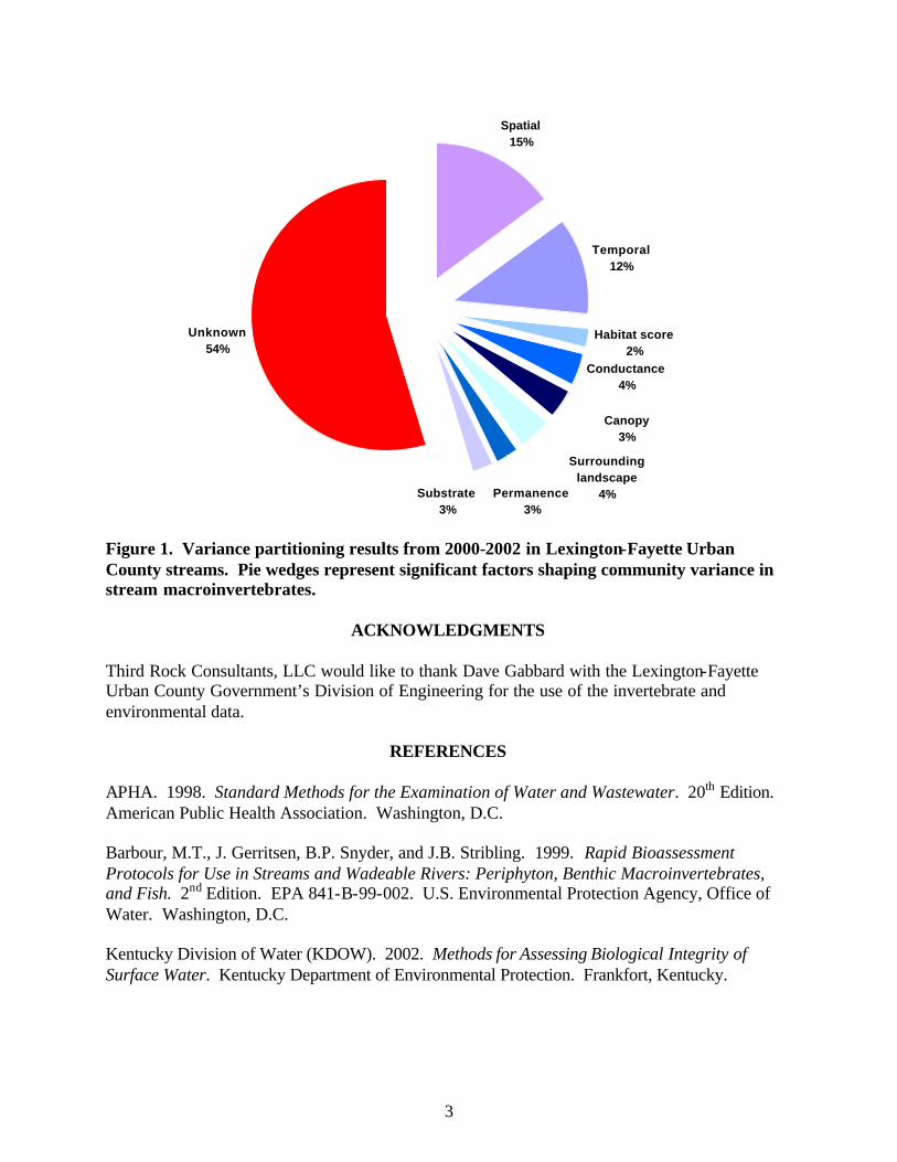
RESULTS AND DISCUSSION Eight environmental variables were found to be significantly correlated with invertebrate community fluctuations from the sampled streams. These variables include temporal and spatial effects (time of sampling and area differences), physical habitat scores, specific conductance, canopy closure, surrounding landscape use, stream permanence, and in-stream substrate composition. The variance attributed to each variable is presented in Figure 1. The measured environmental parameters accounted for 46% of the variance in the stream invertebrate community. The community primarily varied spatially (between drainages) and temporally (between sampling periods). A large portion of the variance (55%) was not accounted for. We estimate that the majority of unexplained variation seen in the pie chart was attributed to natural distributional effects that are unquantifiable. Even with such a large percentage of the community variance unaccounted for, these results offer insight to the overall watershed integrity. The measured empirical variables (e.g., canopy closure, habitat score, surrounding landscape composition, etc.) are primarily representative of landscape alteration. This was expected due to the proximity of the sampling sites to the urban area of Lexington. Computed metrics (i.e., modified Hilsenhoff Biotic Index) reinforced this finding by indicating that most of the sampled streams were “poor” in regards to the macroinvertebrate communities (with an exception of the reference stream). Results of this preliminary test indicate that remediation efforts would be best concentrated on physical habitat stabilization and the creation of vegetation buffers. The presentation of multivariate results in a simplistic chart allows for easy interpretation by untrained personnel (e.g., managers, politicians, general public, etc.). The pollutant of concern can be identified and then specifically targeted by resource managers to create management plans to correct watershed-scale problems in an efficient manner. Ease of interpretation can facilitate understanding of complex ecological interactions that can lead to a wider acceptance and support for watershed remediation.

3

Figure 1. Variance partitioning results from 2000-2002 in Lexington-Fayette Urban County streams. Pie wedges represent significant factors shaping community variance in stream macroinvertebrates.

ACKNOWLEDGMENTS Third Rock Consultants, LLC would like to thank Dave Gabbard with the Lexington-Fayette Urban County Government’s Division of Engineering for the use of the invertebrate and environmental data.

REFERENCES APHA. 1998. Standard Methods for the Examination of Water and Wastewater. 20th Edition. American Public Health Association. Washington, D.C. Barbour, M.T., J. Gerritsen, B.P. Snyder, and J.B. Stribling. 1999. Rapid Bioassessment Protocols for Use in Streams and Wadeable Rivers: Periphyton, Benthic Macroinvertebrates, and Fish. 2nd Edition. EPA 841-B-99-002. U.S. Environmental Protection Agency, Office of Water. Washington, D.C. Kentucky Division of Water (KDOW). 2002. Methods for Assessing Biological Integrity of Surface Water. Kentucky Department of Environmental Protection. Frankfort, Kentucky.

Spatial15%

Temporal12%

Habitat score2%

Unknown54%

Conductance4%

Canopy3%

Surrounding landscape

4%Permanence3%

Substrate3%

4

SENSITIVITY OF THE REFERENCE WATERSHED APPROACH IN BENTHIC TMDLS

Rachel Wagner and Theo A. Dillaha

Department of Biological Systems Engineering, Virginia Tech Blacksburg, VA 24061

racain@vt.edu KEY WORDS: benthic, TMDL, modeling, reference watershed

ABSTRACT The most commonly used tool to meet the biological integrity requirements of the Clean Water Act is biomonitoring. When the biota of a water body is impaired, the TMDL process is initiated. Within this process, the primary stressors are determined. This paper will examine the reference watershed approach used for benthic TMDLs. A benthically unimpaired reference watershed is chosen for comparison to the impaired watershed, since no standard exists for many of the stressors. What are the consequences when different reference watersheds are used? This question will be evaluated for the benthically impaired Stroubles Creek in Montgomery County, Virginia.

INTRODUCTION When the Clean Water Act stated the goal to “restore and maintain the chemical, physical, and biological integrity of all navigable waters, ground waters, waters of the contiguous zone, and the oceans” (CWA Section 304a, USEPA 2002), biological monitoring in aquatic systems was established in the water quality regulations of the United States. Scientists have long recognized the advantages of studying the biota of a water body over the chemical components. While a chemical assessment of a stream takes a snapshot of the water quality at the moment sampled, a biological assessment demonstrates a more extensive temporal picture, since the effects of pollution on the biological community are longer- lived. Perhaps a stream receives a slug of a chemical pollutant in a highly toxic amount, but the pollutant is quickly washed downstream. Chemical monitoring after the pollutant is washed downstream will not indicate a problem, but the biological community will show the affects (Walker et al. 2002). In contrast, a chemical sample may catch a pollutant at measurably high concentrations, but not at concentrations high enough to cause a biological problem. Since the goal of biological monitoring “should be to detect significant changes in ecosystems, not minor fluctuations that are quickly dampened,” the biota in this second example is again the preferred indicator of problems for the stream ecosystem (Cairns and Pratt 1993). It is not surprising, therefore, that the biological community is considered “one of the best indicators of potential for beneficial use of a water resource” (Karr 1989). In addition to being a better indicator of long-term degradation of a water body, the biological community is important in regulating pollutants and environmental stressors that do not have

5

defined water quality standards. In these instances, biological indicators can serve as “sentinels” for a water quality problem that is not defined by a chemical standard. Non-native species, flow regime changes, and sedimentation are examples of pollutants or environmental stressors with no standards (USEPA 2000). All three, however, can have detrimental effects on biota and therefore indicate a failure to comply with the Clean Water Act. In Virginia, benthic macroinvertebrates are used as the primary indicator of the health of the stream biota. When the benthic macroinvertebrate assemblage of a given water body is not deemed healthy, the TMDL (total maximum daily load) process is initiated. The National Research Council, in their 2001 assessment of the TMDL process, writes, “in general, biological criteria are more closely related to the designated uses of waterbodies than are physical or chemical measurements” (NRC 2001). Virginia’s two biologically-related designated uses, preservation of a naturally extant fish population and safe human contact with water, require enforcement of ecosystem management to maintain the ecological services desired. Biological monitoring is the best way to ensure that these designated uses are maintained. The benthic community is an indicator that a problem is present in the stream, but the biota does not pinpoint the specific problem (USEPA 2000). Sometimes the number and type of organisms present in an assemblage (the “metrics”) can offer clues to the cause of the impairment, but they do not reveal a definite answer. Therefore, other data available, such as dissolved oxygen, habitat quality, and nutrient information must be analyzed in conjunction with the benthic metrics. This part of the benthic TMDL process, in which the cause(s) of the benthic impairment are determined, is called the Stressor Analysis process. Often, no single parameter stands out as a clear candidate for the cause of the problem. Stressor Analysis compiles data from the benthic metrics, the chemical ambient water quality measurements, and the physical habitat evaluations to determine which stressors will be targeted for the TMDL. Once the stressor(s) is identified, it can be difficult to determine the reductions of (or changes to) that stressor that are necessary to restore the benthic community. For many of these parameters, such as sediment and nutrients, there are no water quality standards in Virginia. Therefore, a different method is required to determine those reductions. Currently, all the approved benthic TMDLs in Virginia have been handled with the reference watershed approach. In this method, a watershed is located that has similar characteristics (e.g., ecoregion, land use, climate) to the impaired watershed, but the reference watershed does not exhibit a benthic impairment. The loading of a stressor(s) in the reference watershed is established as the target level for the stressor(s) in the impaired watershed. It is expected that if the stressor load(s) in the impaired watershed can be reduced to the level(s) in the reference watershed, then the benthic community in the impaired watershed should be restored over time. Calculating the loadings of the stressor(s) in the impaired watershed and the reference watershed is usually accomplished using computer models. Computer models exist for watershed processes, such as sediment and nutrient transport into and within a stream. The models are based on mathematical equations that predict these processes. Models are available with different levels of complexity based on the user’s needs and on the available data. Typically one model, such as the General Watershed Loadings Function model (GWLF), is chosen to determine the loading of the stressor (e.g., sediment or nutrients) into the water body. The

6

loadings are calculated based on the mathematical equations within the model and the characteristics of the watershed, which are inputs to the model. The TMDL process ends with a determination of the necessary reductions of (or changes to) the targeted stressor(s) within the watershed. In the implementation process, how and where the reductions can be made most efficiently and effectively are calculated, and a plan is developed to make the physical changes within the watershed that are necessary to achieve the reductions. Best management practices, such as restricting cattle access to a stream or planting vegetative filter strips, are common tools in implementation. Following implementation, continued monitoring must occur to determine if the TMDL process and its implementation have successfully restored the benthic community. The organisms in the benthic assemblage may take a long time (years to decades) to return to the water body and establish communities representative of a healthy water body. Therefore, monitoring of chemical and physical characteristics that respond to implementation more quickly than the biota can indicate if a long-term trend is in place to restore the biological community. The ultimate goal of the benthic TMDL, however, is not chemical or physical, but rather the restoration of a healthy benthic community in the water body.

METHODS

The reference watershed approach as described above poses some concerns. Although the watershed chosen to be a reference should be similar to the impaired watershed, it is often difficult to find a watershed that is a “perfect” reference. Multiple candidates are usually available, each with their own set of compromises in matching the impaired watershed. For the current reference watershed approach in Virginia, only one watershed is chosen to determine the target load for the stressor. What differences might comparisons between the impaired watershed and different reference watersheds demonstrate? Furthermore, how different would the necessary reductions in the impaired watershed be if they are based on different reference watersheds? If the selection of reference watersheds results in widely differing target loads, the implications for the changes necessary in the impaired watershed could be significant. How should the benthic TMDL process handle these differences? Examination of the research questions will be based on the benthically impaired Stroubles Creek, a tributary of the New River. Located in Montgomery County, Virginia, the Stroubles Creek watershed (VAW-N22R, HUC 05050001; approximately 6,119 acres) encompasses much of the town of Blacksburg. Biological monitoring of Stroubles Creek over a period of five years has indicated that the water body does not support the general standard of water quality in Virginia. For Stroubles Creek, the assessment period for 2002 was from January 1996 to January 2001. During this period, Stroubles Creek’s benthic community was monitored nine times; each assessment received a moderately impaired rating, resulting in a violation of the general standard. Due to these water quality violations, Stroubles Creek has been placed on Virginia’s 2002 303(d) list of impaired water bodies for benthic impairment. The impairment starts at the headwaters and continues downstream to its confluence with Wall’s Branch, for a total of 7.28 stream miles.

7

Physical and chemical monitoring of Stroubles Creek during the 2002 assessment period occurred at an ambient water quality monitoring station approximately five miles downstream from the biological monitoring station. Data from this sampling does not clearly identify a single stressor acting on the benthic community. Stressor Analysis is currently in progress for Stroubles Creek. The primary candidates for stressors on its benthic community appear to be sediment, nutrients, and organic matter. Once the stressor(s) has been confirmed, the TMDL process will continue. The research into reference watershed comparison will be performed using sediment as the primary stressor.

REFERENCES Cairns, John and James Pratt. 1993. A history of biological monitoring using benthic macroinvertebrates. In: Freshwater Biomonitoring and Benthic Macroinvertebrates. D. M. Rosenberg and V.R. Resh (Editors). Chapman and Hall. New York, N.Y. pp. 10-27. Karr, James R. October 16-19, 1989. Bioassessment and non-point source pollution: An overview. In: National Symposium on Water Quality Assessment. Fort Collins, Colo. National Research Council (NRC). 2001. Assessing the TMDL Approach to Water Quality Management. National Academy Press. Washington, D.C. http://www.nap.edu/books/0309075793/html/ (1/2003). U.S. Environmental Protection Agency (USEPA). 2000. Stressor Identification Guidance Document. EPA 822-B-00-025. Office of Water and Office of Research and Development. Washington, D.C. U.S. Environmental Protection Agency (USEPA). 2002. Clean Water Act. http://www.epa.gov/r5water/cwa.htm (1/2003). Walker, Jane, Kimberly Porter, and Tamim Younos. 2002. Monitoring needs to meet benthic TMDL requirements. In: National Water Quality Monitoring Council National Monitoring Conference. Madison, Wis.

8

TOTAL MAXIMUM DAILY LOAD DEVELOPMENT FOR LINVILLE CREEK–BACTERIA AND GENERAL STANDARD (BENTHIC) IMPAIRMENTS:

A CASE STUDY

S. Mostaghimi, B. Benham, K. Brannan, J. Wynn, G. Yagow, and R. Zeckoski Department of Biological Systems Engineering, Virginia Tech

209 Seitz Hall (0303), Blacksburg, VA 24061 benham@vt.edu

KEY WORDS: TMDL, water quality, bacteria, benthic

ABSTRACT Two TMDLs were developed for Linville Creek, a general standard (benthic) TMDL and a bacteria TMDL. Sediment is the primary stressor affecting the benthic community in Linville Creek. Virginia has no numeric water quality criterion for sediment. As a result, the benthic TMDL utilized a reference watershed to establish the TMDL target load. The sediment TMDL requires a load reduction of 12.3%. Virginia recently adopted an Escherichia coli (E. coli) standard for bacteria impairments. The E. coli standard is more restrictive than the previous standard. The E. coli allocation for Linville Creek requires a load reduction of 96% compared to the existing load.

INTRODUCTION The Commonwealth of Virginia and EPA are mandated under a 1998 consent decree to develop 636 TMDL plans by 2010. Most of the impairments to be addressed in these plans are due to nonpoint source (NPS) pollution. The case study presented here discusses the Linville Creek TMDL developed by Virginia Tech’s Biological Systems Engineering Department. Linville Creek, located in Rockingham County, Virginia, is a predominantly rural watershed with beef, dairy, poultry, and row crop production operations. Linville Creek is listed as impaired on Virginia’s 1998 Section 303(d) Total Maximum Daily Load Priority List and Report for water quality violations of both the Bacteria Standard and the General Standard for Aquatic Life Use (listed as a benthic impairment). This paper discusses the development of the Linville Creek TMDLs. The final allocation scenarios are also presented, and the associated implications of those scenarios are discussed.

TMDL DEVELOPMENT Benthic TMDL: The stressor identification analysis of Linville Creek water quality data indicated that sediment was the primary pollutant affecting the benthic community. Currently, Virginia has no numeric water quality criterion for sediment. Therefore, a reference watershed approach was used to establish the target sediment load. The reference watershed for Linville Creek was the Upper Opequon Creek watershed. The GWLF model, originally developed for use in ungaged watersheds (Haith et al. 1992), was used to model both watersheds. However, the BasinSim adaptation of the model (Dai et al. 2000) recommends hydrologic calibration of the

9

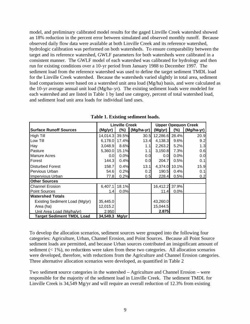
model, and preliminary calibrated model results for the gaged Linville Creek watershed showed an 18% reduction in the percent error between simulated and observed monthly runoff. Because observed daily flow data were available at both Linville Creek and its reference watershed, hydrologic calibration was performed on both watersheds. To ensure comparability between the target and its reference watershed, GWLF parameters for both watersheds were calibrated in a consistent manner. The GWLF model of each watershed was calibrated for hydrology and then run for existing conditions over a 10-yr period from January 1988 to December 1997. The sediment load from the reference watershed was used to define the target sediment TMDL load for the Linville Creek watershed. Because the watersheds varied slightly in total area, sediment load comparisons were based on a watershed unit area load (Mg/ha) basis, and were calculated as the 10-yr average annual unit load (Mg/ha-yr). The existing sediment loads were modeled for each watershed and are listed in Table 1 by land use category, percent of total watershed load, and sediment load unit area loads for individual land uses.

Table 1. Existing sediment loads.

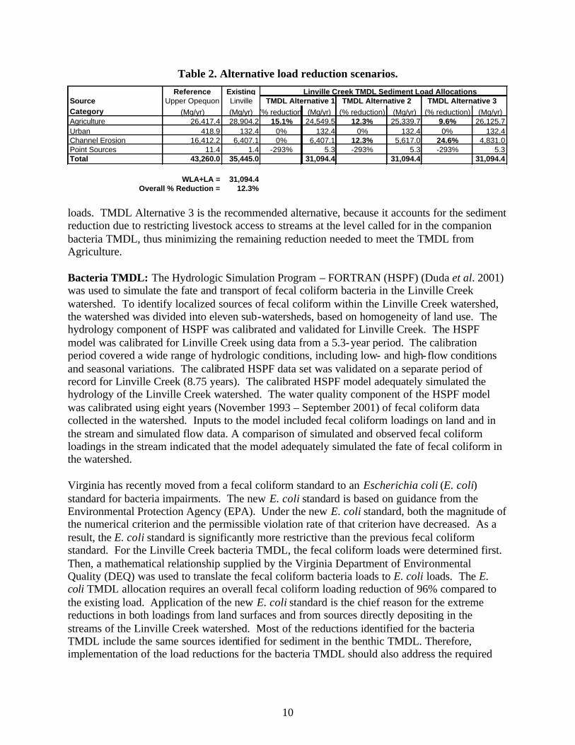
Linville Creek Upper Opequon CreekSurface Runoff Sources (Mg/yr) (%) (Mg/ha-yr) (Mg/yr) (%) (Mg/ha-yr)High Till 14,014.3 39.5% 30.5 12,286.6 28.4% 20.9Low Till 6,178.0 17.4% 13.4 4,138.3 9.6% 9.2Hay 3,048.9 8.6% 1.1 2,263.2 5.2% 1.3Pasture 5,360.0 15.1% 1.1 3,150.8 7.3% 0.6Manure Acres 0.0 0.0% 0.0 0.0 0.0% 0.0Forest 144.3 0.4% 0.0 204.7 0.5% 0.1Disturbed Forest 158.7 0.4% 13.1 4,374.0 10.1% 15.9Pervious Urban 54.6 0.2% 0.2 190.5 0.4% 0.1Impervious Urban 77.8 0.2% 0.5 228.4 0.5% 0.2Other SourcesChannel Erosion 6,407.1 18.1% 16,412.2 37.9%Point Sources 1.4 0.0% 11.4 0.0%Watershed Totals Existing Sediment Load (Mg/yr) 35,445.0 43,260.0 Area (ha) 12,015.2 15,044.5 Unit Area Load (Mg/ha/yr) 2.950 2.875 Target Sediment TMDL Load 34,549.3 Mg/yr To develop the allocation scenarios, sediment sources were grouped into the following four categories: Agriculture, Urban, Channel Erosion, and Point Sources. Because all Point Source sediment loads are permitted, and because Urban sources contributed an insignificant amount of sediment (< 1%), no reductions were taken from these two categories. All allocation scenarios were developed, therefore, with reductions from the Agriculture and Channel Erosion categories. Three alternative allocation scenarios were developed, as quantified in Table 2 Two sediment source categories in the watershed – Agriculture and Channel Erosion – were responsible for the majority of the sediment load in Linville Creek. The sediment TMDL for Linville Creek is 34,549 Mg/yr and will require an overall reduction of 12.3% from existing

10

Table 2. Alternative load reduction scenarios. Reference Existing Linville Creek TMDL Sediment Load Allocations

Source Upper Opequon Linville TMDL Alternative 1 TMDL Alternative 2 TMDL Alternative 3Category (Mg/yr) (Mg/yr) (% reduction) (Mg/yr) (% reduction) (Mg/yr) (% reduction) (Mg/yr)Agriculture 26,417.4 28,904.2 15.1% 24,549.5 12.3% 25,339.7 9.6% 26,125.7Urban 418.9 132.4 0% 132.4 0% 132.4 0% 132.4Channel Erosion 16,412.2 6,407.1 0% 6,407.1 12.3% 5,617.0 24.6% 4,831.0Point Sources 11.4 1.4 -293% 5.3 -293% 5.3 -293% 5.3Total 43,260.0 35,445.0 31,094.4 31,094.4 31,094.4

WLA+LA = 31,094.4Overall % Reduction = 12.3%

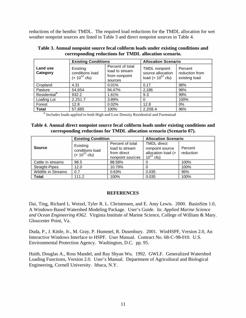
loads. TMDL Alternative 3 is the recommended alternative, because it accounts for the sediment reduction due to restricting livestock access to streams at the level called for in the companion bacteria TMDL, thus minimizing the remaining reduction needed to meet the TMDL from Agriculture. Bacteria TMDL: The Hydrologic Simulation Program – FORTRAN (HSPF) (Duda et al. 2001) was used to simulate the fate and transport of fecal coliform bacteria in the Linville Creek watershed. To identify localized sources of fecal coliform within the Linville Creek watershed, the watershed was divided into eleven sub-watersheds, based on homogeneity of land use. The hydrology component of HSPF was calibrated and validated for Linville Creek. The HSPF model was calibrated for Linville Creek using data from a 5.3-year period. The calibration period covered a wide range of hydrologic conditions, including low- and high-flow conditions and seasonal variations. The calibrated HSPF data set was validated on a separate period of record for Linville Creek (8.75 years). The calibrated HSPF model adequately simulated the hydrology of the Linville Creek watershed. The water quality component of the HSPF model was calibrated using eight years (November 1993 – September 2001) of fecal coliform data collected in the watershed. Inputs to the model included fecal coliform loadings on land and in the stream and simulated flow data. A comparison of simulated and observed fecal coliform loadings in the stream indicated that the model adequately simulated the fate of fecal coliform in the watershed. Virginia has recently moved from a fecal coliform standard to an Escherichia coli (E. coli) standard for bacteria impairments. The new E. coli standard is based on guidance from the Environmental Protection Agency (EPA). Under the new E. coli standard, both the magnitude of the numerical criterion and the permissible violation rate of that criterion have decreased. As a result, the E. coli standard is significantly more restrictive than the previous fecal coliform standard. For the Linville Creek bacteria TMDL, the fecal coliform loads were determined first. Then, a mathematical relationship supplied by the Virginia Department of Environmental Quality (DEQ) was used to translate the fecal coliform bacteria loads to E. coli loads. The E. coli TMDL allocation requires an overall fecal coliform loading reduction of 96% compared to the existing load. Application of the new E. coli standard is the chief reason for the extreme reductions in both loadings from land surfaces and from sources directly depositing in the streams of the Linville Creek watershed. Most of the reductions identified for the bacteria TMDL include the same sources identified for sediment in the benthic TMDL. Therefore, implementation of the load reductions for the bacteria TMDL should also address the required

11

reductions of the benthic TMDL. The required load reductions for the TMDL allocation for wet weather nonpoint sources are listed in Table 3 and direct nonpoint sources in Table 4.

Table 3. Annual nonpoint source fecal coliform loads under existing conditions and corresponding reductions for TMDL allocation scenario.

Existing Conditions Allocation Scenario

Land use Category

Existing conditions load (× 1012 cfu)

Percent of total load to stream from nonpoint sources

TMDL nonpoint source allocation load (× 1012 cfu)

Percent reduction from existing load

Cropland 4.31 0.01% 0.17 96% Pasture 54,654 94.47% 2,186 96% Residentiala 932.2 1.61% 9.3 99% Loafing Lot 2,251.7 3.89% 0 100% Forest 12.8 0.02% 12.8 0% Total 57,885 100% 2,208.4 96%

a Includes loads applied to both High and Low Density Residential and Farmstead Table 4. Annual direct nonpoint source fecal coliform loads under existing conditions and

corresponding reductions for TMDL allocation scenario (Scenario 07).

Existing Condition Allocation Scenario

Source Existing conditions load (× 1012 cfu)

Percent of total load to stream from direct nonpoint sources

TMDL direct nonpoint source allocation load (× 1012 cfu)

Percent reduction

Cattle in streams 98.5 88.58% 0 100% Straight-Pipes 12.0 10.79% 0 100% Wildlife in Streams 0.7 0.63% 0.035 95% Total 111.2 100% 0.035 100%

REFERENCES Dai, Ting, Richard L. Wetzel, Tyler R. L. Christensen, and E. Amy Lewis. 2000. BasinSim 1.0, A Windows-Based Watershed Modeling Package. User’s Guide. In: Applied Marine Science and Ocean Engineering #362. Virginia Institute of Marine Science, College of William & Mary. Gloucester Point, Va. Duda, P., J. Kittle, Jr., M. Gray, P. Hummel, R. Dusenbury. 2001. WinHSPF, Version 2.0, An Interactive Windows Interface to HSPF. User Manual. Contract No. 68-C-98-010. U.S. Environmental Protection Agency. Washington, D.C. pp. 95. Haith, Douglas A., Ross Mandel, and Ray Shyan Wu. 1992. GWLF. Generalized Watershed Loading Functions, Version 2.0. User’s Manual. Department of Agricultural and Biological Engineering, Cornell University. Ithaca, N.Y.

12

QUANTIFYING NONPOINT SOURCE (NPS) POLLUTANT DELIVERY IN AN URBANIZING HEADWATER BASIN

Mark Dougherty and Randel L. Dymond

Department of Civil and Environmental Engineering, Virginia Tech Blacksburg, VA 24061

mdougher@vt.edu

Carl E. Zipper Department of Crop and Soil Environmental Sciences, Virginia Tech

Blacksburg, VA 24061 KEY WORDS: NPS flux, urbanization, storm, precipitation

INTRODUCTION In spite of several national nonpoint source (NPS) studies (U.S.EPA 1983, Driver and Tasker 1988), research in diffuse pollution that includes both urban and rural sources has been on the fringe of environmental engineering research (Novotny 1999). A number of studies have measured pollutant fluxes from large mixed land use watersheds. These studies have demonstrated the importance of land use management in controlling the magnitude of total suspended solids (TSS)-related fluxes and show that most TSS fluxes occur during large or intense storm events. However, few studies in literature have the combined long-term precipitation and integrated pollutant discharge data necessary to evaluate NPS pollutant flux as a function of precipitation (Correll et al. 1999a). This research investigates fundamental watershed relationships using a unique assembly of long-term spatial and water quality data. The study area consists of four headwater catchments in the Piedmont physiographic province of the Chesapeake Bay drainage. The basins are part of the 1530 km2 Occoquan River watershed in northern Virginia (Figure 1). The three western basins, ranging in size from 67 to 400 km2, are predominantly forest and/or mixed agriculture. The fourth basin, the 127 km2 Cub Run watershed, is rapidly urbanizing, with 17% impervious surface and 50% of current land use classed as urban. Metcalf & Eddy (1970) determined that a major cause of water quality impairment in the Occoquan Reservoir (Figure 2) was nutrients, particularly phosphorus, from separate sewage treatment plants and from forested, agricultural, and urban lands. Water supply protection began in 1971 through replacement of the watershed’s 11 sewage treatment works with a single advanced wastewater treatment (AWT) plant and the establishment of the Occoquan Watershed Monitoring Program and Laboratory (OWML) (Randall and Grizzard 1995). Early results from the monitoring program established nonpoint nutrient pollution as a major cause of water quality impairment. The AWT went on line in July of 1978, effectively removing point source contributions in the Cub Run basin. Continued monitoring has demonstrated that ongoing control of both point and nonpoint nutrients is necessary to protect the water quality of the Occoquan reservoir.

13

Figure 1. Location map: Occoquan River watershed study area, northern Virginia, USA.

The present study uses a unique combination of long-term data, including: over 30 years of integrated stream flow and water chemistry data from four OWML headwater monitoring stations (Figure 2); over 50 years of daily precipitation data from nine local rain gages; over 30 years of daily stream discharge data; 20 years of land use mapping from the Northern Virginia Regional Commission (NVRC); and 14 years of remotely-sensed impervious surface estimates at 30 meter resolution from the Mid-Atlantic Regional Earth Science Applications Center (RESAC). The above data sets have been described previously by Dougherty et al. (2002).

Figure 2. Occoquan basin (1530 sq. km): Relief map showing four headwater basins, Occoquan reservoir, and major water monitoring stations.

Cub Run basin Upper Bull Run basin

Upper Broad Run basin

Cedar Run basin

Occoquan reservoir

14

METHODS This study analyzes long-term annual precipitation, stream discharge, total suspended solids, total phosphorus, and total nitrogen fluxes in four headwater basins of the Occoquan River. Basins are absent significant, known point source contributions during the 22-year study period (1979-2000). The basin outlets were monitored with automated daily discharge and flow-proportional, volume-integrating storm samplers, and with discrete weekly grab samples for characterization of non-storm flows. A total of 88 basin-years are available for study (4 basins x 22 years). Basin-years with greater than 90 consecutive days of missing water quality samples are deleted. The remaining 76 basin-years have, on average, 33 discrete non-storm samples and 17 composite storm samples per year. Missing flow data are infilled using the drainage area ratio method (Johnston 1999) with adjacent gaged basins. Missing constituent concentrations are infilled using corresponding seasonal medians for each constituent and basin. Annual NPS pollutant loads are estimated as the product of flow times concentration using a modified OWML method (Johnston 1999) to sum independently-calculated storm and non-storm loads. Initial annual load estimates are adjusted based upon comparison of estimated annual flows with the actual daily flow record. Annual load estimates are adjusted upward or downward using historic constituent means (Table 1) times the difference of estimated annual flow from the actual daily flow record. Precipitation, stream discharge, and NPS pollutant loads are normalized by basin area for further analysis.

Table 1. Historic constituent means for annual load adjustment, mg/L.

Basin Mean TP Mean TSS Mean TN Cedar Run 0.13 40.27 1.42 Cub Run 0.12 77.68 1.34 Upper Bull Run 0.12 58.88 1.18 Upper Broad Run 0.10 38.96 1.14

In each basin, the relationship of runoff to rainfall is evaluated as a function of season and landscape in order to assess hydrologic patterns across time. Annual NPS pollutant fluxes are plotted against changing precipitation and discharge conditions in order to provide a long-term perspective on the potential for change due to urbanization.

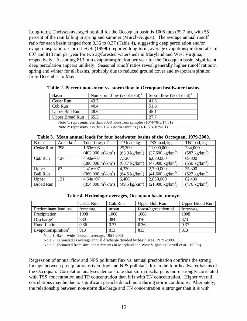
RESULTS AND DISCUSSION Mean storm flow volume as a percent of total annual flow volume is greater than non-storm flow volume only in Cub Run, the most highly urbanized basin (Table 2). Total drainage area from the four headwater basins makes up approximately 47% of the Occoquan basin. Annual loads from the four basins made up, on average, 40% of total Occoquan basin NPS pollutant loads, with total flows and loads generally proportional to basin drainage area (Table 3). Comparison of the urbanizing Cub Run basin with the Upper Broad Run basin, however, reveals that Cub Run had more than twice the average TSS load as Upper Broad Run, a similar-sized basin. Cub Run basin had 9% greater average annual flow volumes and 23% and 16% greater annual TP and TN yields, respectively, than Upper Broad Run basin. Average annual TSS yields for Cub and Upper Bull Run basins were significantly higher than the other ag/forested watersheds.

15

Long-term, Theissen-averaged rainfall for the Occoquan basin is 1008 mm (39.7 in), with 55 percent of the rain falling in spring and summer (March-August). The average annual runoff ratio for each basin ranged from 0.36 to 0.37 (Table 4), suggesting deep percolation and/or evapotranspiration. Correll et al. (1999b) reported long-term, average evapotranspiration rates of 807 and 818 mm per year for two ag/forested watersheds in Maryland and West Virginia, respectively. Assuming 813 mm evapotranspiration per year for the Occoquan basin, significant deep percolation appears unlikely. Seasonal runoff ratios reveal generally higher runoff ratios in spring and winter for all basins, probably due to reduced ground cover and evapotranspiration from December to May.

Table 2. Percent non-storm vs. storm flow in Occoquan headwater basins.

Basin Non-storm flow (% of total)1 Storm flow (% of total)2 Cedar Run 43.5 41.3 Cub Run 40.4 51.8 Upper Bull Run 48.6 45.1 Upper Broad Run 65.3 27.7

Note 1: represents less than 3058 non-storm samples (10/4/78-5/14/01) Note 2: represents less than 1523 storm samples (11/18/78-3/29/01)

Table 3. Mean annual loads for four headwater basins of the Occoquan, 1979-2000. Basin Area, km2 Total flow, m3 TP load, kg TSS load, kg TN load, kg Cedar Run 398 1.60e+08

(402,000 m3/km2) 25,200 (63.3 kg/km2)

11,000,000 (27,600 kg/km2)

234,000 (587 kg/km2)

Cub Run 127 4.90e+07 (386,000 m3/km2)

7,720 (60.7 kg/km2)

6,080,000 (47,900 kg/km2)

69,800 (550 kg/km2)

Upper Bull Run

67 2.41e+07 (360,000 m3/km2)

4,320 (64.5 kg/km2)

2,790,000 (41,600 kg/km2)

35,300 (527 kg/km2)

Upper Broad Run

131 4.64e+07 (354,000 m3/km2)

6,480 (49.5 kg/km2)

2,860,000 (21,900 kg/km2)

62,400 (476 kg/km2)

Table 4. Hydrologic averages, Occoquan basin, mm/yr.

Cedar Run Cub Run Upper Bull Run Upper Broad Run Predominant land use forest/ag urban forest/ag/residential forest/ag Precipitation1 1008 1008 1008 1008 Discharge2 380 384 376 373 Runoff ratio 0.36 0.37 0.36 0.37 Evapotranspiration3 813 813 813 813

Note 1: Basin-wide Theissen average, 1951-2002. Note 2: Estimated as average annual discharge divided by basin area, 1979-2000. Note 3: Estimated from similar catchments in Maryland and West Virginia (Correll et al.. 1999b).

Regression of annual flow and NPS pollutant flux vs. annual precipitation confirms the strong linkage between precipitation-driven flow and NPS pollutant flux in the four headwater basins of the Occoquan. Correlation analyses demonstrate that storm discharge is more strongly correlated with TSS concentration and TP concentration than it is with TN concentration. Higher overall correlations may be due to significant particle detachment during storm conditions. Alternately, the relationship between non-storm discharge and TN concentration is stronger than it is with

16

either TSS or TP concentration, suggesting a predominance of soluble nitrogen forms in non-storm flows. Storm and non-storm flow partitions suggest that NPS storm fluxes in these mixed land use basins are laden with particulate constituents, while non-storm fluxes are more closely associated with dissolved constituents.

CONCLUSIONS This research quantifies nonpoint source sediment and nutrient fluxes from four headwater basins in the Piedmont physiographic province of the Chesapeake Bay drainage for up to 22 years. Only one of the basins, the 127 km2 Cub Run watershed, is rapidly urbanizing. Basin outlets were monitored for characterization of seasonal and annual flows, along with annual fluxes of total suspended solids and total phosphorus and nitrogen. Results indicate strong correlations between annual and seasonal stream discharge and precipitation, annual NPS pollutant loads and precipitation, and TSS and TP concentrations with storm flow. Cub Run basin had disproportionately higher TSS loads and a majority of total flow as storm flow.

ACKNOWLEDGMENTS The authors gratefully acknowledge the financial support of the Virginia Water Resources Research Center and the Charles E. Via, Jr. Department of Civil & Environmental Engineering. Collaborative support from the Occoquan Watershed Monitoring Laboratory, the Northern Virginia Regional Commission, and the Mid-Atlantic Regional Earth Science Applications Center provided the data for this study.

REFERENCES Correll, D.L., Jordan, T.E., and D.E. Weller. 1999a. Precipitation effects on sediment and associated nutrient discharges from Rhode River. J. Env. Qual. 28(6): 1897-1907. Correll, D.L., Jordan, T.E., and D.E. Weller. 1999b. Effects of interannual variation of precipitation on stream discharge from Rhode River watersheds. Journal of the American Water Resources Association 35(1): 73-81. Dougherty, M., Dymond, R.L., Grizzard, T.J., Godrej, A.N., and C.E. Zipper. 2002. Evaluation of land use and population change on pollutant delivery from an urbanizing watershed. In: Proceedings Virginia Water Resources Symposium 2002, Nov. 6-7, 2002, Richmond, Va. Driver, N.E. and G.D. Tasker. 1988. Techniques for Estimation of Storm-runoff Loads, Volumes, and Selected Constituent Concentrations in Urban Watersheds in the United States. Open-file report 88-191. U.S. Geological Survey. Denver, Colo. Johnston, C.A. 1999. Development and Evaluation of Infilling Methods for Missing Hydrologic and Chemical Watershed Data. M.S. Thesis. Virginia Tech. Blacksburg, Va. Metcalf & Eddy, Inc. 1970. 1969 Occoquan Reservoir Study. Completed for the Commonwealth of Virginia State Water Control Board. April 1970.

17

Novotny, V. 1999. Integrating diffuse/nonpoint pollution control and water body restoration into watershed management. J. Amer. Wat. Res. Assoc. 35(4): 717-727. Randall, C. W. and T.J. Grizzard. 1995. Management of the Occoquan River basin: a 20-year case history. Water Science & Technology 32(5-6): 235-243. U.S. EPA. 1983. Results of the Nationwide Urban Runoff Program. Volume I -Final Report. NTIS PB84-185552. Water Planning Division, WH-554. Washington, D.C.

18

U.S. GEOLOGICAL SURVEY ON-LINE FLUVIAL SEDIMENT DATA

John R. Gray U.S. Geological Survey

415 National Center, Reston, VA 20192 jrgray@usgs.gov

Lisa M. Turcios

Dewberry, 8401 Arlington Blvd, Fairfax, VA 22031-4666

KEY WORDS: database, water quality, fluvial sediment, suspended sediment, bedload, bed material

ABSTRACT A retrieval from the U.S. Geological Survey National Water Information System World Wide Web database in 2000 yielded more than 2.6 million values of instantaneous-value sediment and ancillary data for 15,415 sites in all 50 States and other locations. The retrieval included 12,115 sites with suspended-sediment concentration data, about half of which also had particle-size distribution data; 238 sites with bedload-discharge data; and 3,623 sites with bed-material particle-size distribution data. Ancillary variables, including water temperature and discharge, and a large amount of chemical-quality data, also are available. These data, summarized on- line at http://water.usgs.gov/osw/sediment/index.html, represent the single largest repository of U.S. Geological Survey electronic instantaneous suspended-sediment, bedload, and bed-material data.

INTRODUCTION As part of its responsibility to acquire, manage, and disseminate water data to the public (Glysson and Gray 1997), the U.S. Geological Survey (USGS) maintains the National Water Information System (NWIS), a distributed network of computers and fileservers for storing and retrieving water data collected at about 1.5 million sites around the country (U.S. Geological Survey, 2003a). Many types of water and ancillary data are stored in the NWIS, including time-series—flow, stage, precipitation, and selected physical and chemical—data; peak-flow, groundwater, and water-quality data; and associated site information. Water-quality data include the chemical and physical characteristics of natural waters. The latter includes selected characteristics of suspended sediment, bedload, and bed material in surface water. The NWIS on the World Wide Web, termed the “NWISWeb,” provides users of USGS water information with a geographically seamless interface to the large volume of water data maintained nationwide (U.S. Geological Survey 2003b). The NWISWeb water-quality database represents the single largest repository of electronic USGS instantaneous-value sediment and ancillary data. Additionally, daily-value suspended-sediment data collected by the USGS from 1930 through September 30, 1994, are available to the public in a static on- line database (U.S. Geological Survey 2003c).

19

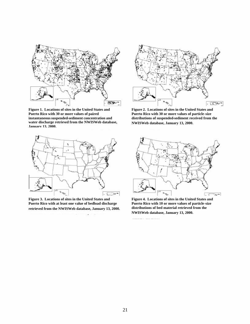
NATIONAL ON-LINE FLUVIAL SEDIMENT AND ANCILLARY DATA More than 2.6 million values of instantaneous-value sediment and ancillary data were retrieved for 15,415 sites in all 50 States, Puerto Rico, and other locations, including Canada, Federated States of Micronesia, Guam, and Southern Ryukyu Islands, from the NWISWeb database on January 13, 2000 (Turcios and Gray 2001; U.S. Geological Survey 2003d). Retrieval results for selected types of instantaneous-value sediment and ancillary data grouped by State or other location are summarized in Table 1. The sediment data were collected by standard USGS protocols and instruments (Edwards and Glysson 1999). A large amount of instantaneous-value water-quality data and descriptive site information was also available at many of the sites, but are not described herein. The data described herein, associated water-quality data, and data added to the database since January 2000 may be retrieved on-line via the “Water Quality Samples for the Nation” (U.S. Geological Survey 2003e). Suspended-Sediment Concentrations: At least one set of values of instantaneous-value suspended-sediment concentration and instantaneous-value water-discharge data was available for 12,115 sites, of which 2,929 had at least 30 such paired values. A map of sites in the United States and Puerto Rico that have at least 30 paired values of instantaneous-value suspended-sediment concentration and water-discharge data are shown in Figure 1. Suspended-Sediment Particle-Size Distributions: Percentages of suspended sand-size and finer material were available for 6,028 sites, of which 1,342 had at least 30 such values. A map of the sites that have at least 30 values of particle-size distribution of suspended sediment is shown in Figure 2. Many sites include more detailed particle-size distribution information. Bedload Discharge: Bedload-discharge values were available for 238 sites, of which 43 had at least 30 values. A map of the sites that have at least one value of bedload discharge is shown in Figure 3. Many of the sites also had particle-size distributions associated with the bedload measurement, such as percentages of material in selected sand- and gravel-size fractions. Particle-Size Distribution of Bed Material: Particle-size distribution values of bed material were available at 3,623 sites, of which 474 had at least 10 values. A map of the sites that have at least 10 values of particle-size distribution of bed material is shown in Figure 4.

VIRGINIA ON-LINE FLUVIAL SEDIMENT AND ANCILLARY DATA At least one set of values of instantaneous-value suspended-sediment concentration and instantaneous-value water-discharge data was available for each of 219 sites in Virginia, of which 31 had at least 30 such paired values (Figure 5). Of those 31 sites, 23 had data on percentages of suspended sand-size and finer material. Sixteen of those sites had at least 30 values sand-size and finer material values (Figure 5). Statistics for the 31 sites with 30 or more paired water discharge and suspended-sediment concentration values, and for the 16 sites with 30 or more sand-size and finer material values are shown in Table 2.

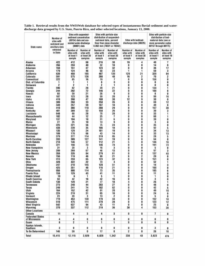
Table 1. Retrieval results from the NWISWeb database for selected types of instantaneous fluvial-sediment and water-discharge data grouped by U.S. State, Puerto Rico, and other selected locations, January 13, 2000.

21

Figure 1. Locations of sites in the United States and Puerto Rico with 30 or more values of paired instantaneous suspended-sediment concentration and water discharge retrieved from the NWISWeb database, January 13, 2000.

Figure 2. Locations of sites in the United States and Puerto Rico with 30 or more values of particle-size distributions of suspended-sediment received from the NWISWeb database, January 13, 2000.

Figure 3. Locations of sites in the United States and Puerto Rico with at least one value of bedload discharge retrieved from the NWISWeb database, January 13, 2000.

Figure 4. Locations of sites in the United States and Puerto Rico with 10 or more values of particle-size distributions of bed material retrieved from the NWISWeb database, January 13, 2000.

22

�: Thirty or more paired instantaneous suspended-sediment concentration and water-discharge values p: Also associated with the sites above, 30 or more suspended-sediment particle-size distribution values

Figure 5. Locations of sites in Virginia with 30 or more values of paired instantaneous suspended-sediment concentration and water discharge; and with 30 or more values of particle-size distributions of suspended-sediment received from the NWISWeb database, January 13, 2000.

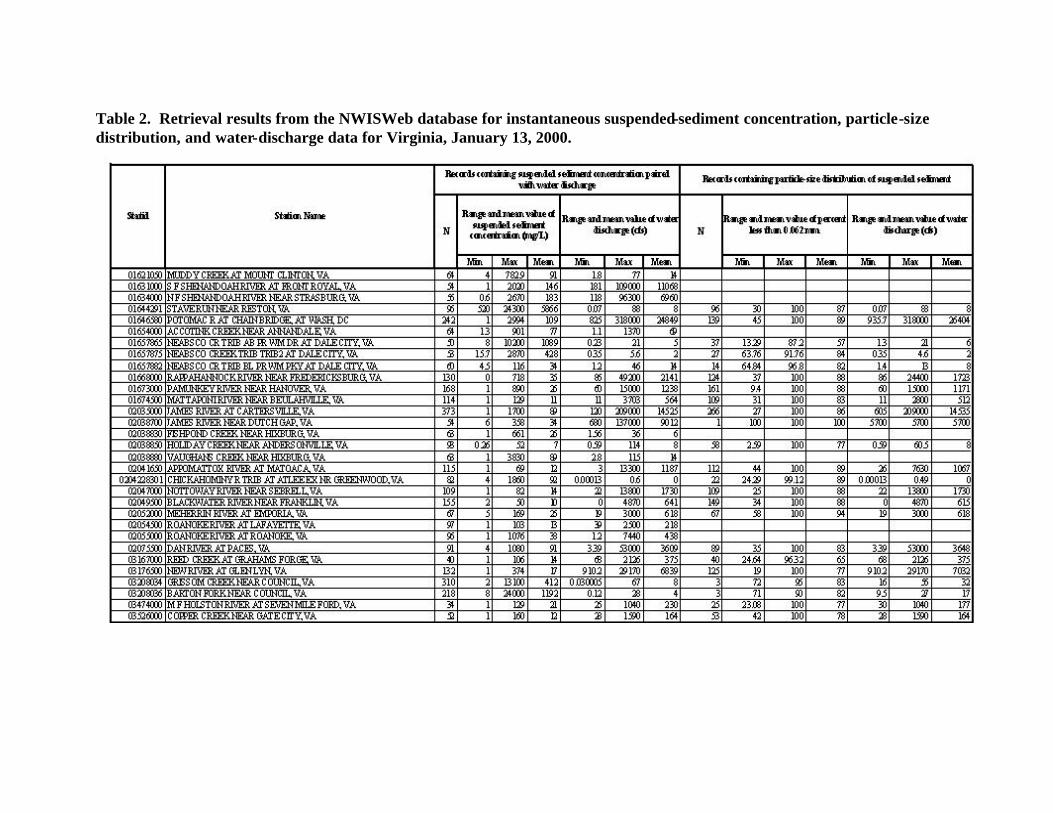
Table 2. Retrieval results from the NWISWeb database for instantaneous suspended-sediment concentration, particle-size distribution, and water-discharge data for Virginia, January 13, 2000.

ACKNOWLEDGMENTS The summary of USGS on- line fluvial sediment described by Turcios and Gray (2001), based on the January 13, 2000, NWISWeb retrieval, was completed in cooperation with the U.S. Environmental Protection Agency’s Office of Wetlands, Oceans, and Watersheds.

REFERENCES CITED Edwards, T.E. and G.D. Glysson. 1999. Field methods for measurement of fluvial sediment. In: U.S. Geological Survey Techniques of Water-Resources Investigations. Report Book 3, Chapter C2. 89 pp. http://water.usgs.gov/osw/techniques/Edwards-TWRI.pdf (May 23, 2003). Glysson, G.D., and J.R. Gray. 1997. Coordination and standardization of federal sedimentation activities. In: Proceedings of the U.S. Geological Survey Sediment Workshop, February 4-7, 1997. http://water.usgs.gov/osw/techniques/workshop/glysson.html (May 23, 2003). Turcios, L.M. and J.R. Gray. 2001. U.S. Geological Survey sediment and ancillary data on the World Wide Web. In: Proceedings of the 7th Federal Interagency Sedimentation Conference, Reno, Nevada, March 25-29. Vol. 1, Poster 31-36. U.S. Geological Survey. 2003a. Water-resources data for USA. http://waterdata.usgs.gov/nwis/ (May 23, 2003). U.S. Geological Survey. 2003b. National Water Information System (NWIS). http://water.usgs.gov/pubs/FS/FS-027-98/ (December 11, 2003). U.S. Geological Survey. 2003c. Suspended-sediment: database: daily values of suspended sediment and ancillary data. http://webserver.cr.usgs.gov/sediment/ (May 23, 2003). U.S. Geological Survey. 2003d. Summary of U.S. Geological Survey on- line fluvial sediment and ancillary data. http://water.usgs.gov/osw/sediment/index.html (June 24, 2003). U.S. Geological Survey. 2003e. Water quality samples for USA. http://water.usgs.gov/nwis/qwdata (May 23, 2003).

25

TOTAL SUSPENDED SOLIDS DATA—A CRITICAL EVALUATION

G. Douglas Glysson U.S. Geological Survey

412 National Center, Reston, VA 20192 gglysson@usgs.gov

John R. Gray

U.S. Geological Survey 415 National Center, Reston, VA 20192

KEY WORDS: total suspended solids, suspended-sediment concentration, bias, quality assurance

ABSTRACT A common measure of the solid-phase concentration of sediments in water—total suspended solids (TSS)—tends to be negatively biased with respect to the quantifiably reliable suspended-sediment concentration (SSC) data type used and sanctioned by the U.S. Geological Survey. Using TSS data to compute loads tends to produce estimates with larger errors than those computed from SSC data. TSS-computed loads tend to be negatively biased with respect to loads computed from SSC data by traditional techniques. A general equation developed to correlate TSS data to SSC data is considered unreliable for correction of TSS data from individual stations.

INTRODUCTION An important measure of water quality is the amount of material suspended in the water. The U.S Geological Survey (USGS) traditionally has used measurements of suspended-sediment concentration (SSC) as the most accurate means for measuring the total amount of suspended material in a water sample collected from open-channel flow. Another commonly used metric is the total suspended solids (TSS) analytical method. The TSS method originally was developed as an analytical technique for use on wastewater samples, but is widely used as a measure of suspended material in stream samples because it is mandated or acceptable for regulatory purposes. This paper summarizes USGS research into the comparability and reliability of SSC and TSS data for use in describing riverine solid-phase concentrations and transport.

DIFFERENCES BETWEEN THE SSC AND TSS ANALYTICAL METHODS Differences between the SSC and TSS analytical methods are associated with sample processing and analysis, and are more or less independent of sample-collection methods. The primary difference between SSC (ASTM 1999) and TSS (American Public Health Association et al. 1995) analytical methods arises from sample processing for subsequent filtering, drying, and weighing. A TSS analysis generally entails withdrawal of an aliquot of the original sample for subsequent analysis, although there is evidence of a lack of consistency in methods used in the

26

sample preparation phase for TSS analyses (Gray et al. 2000). The SSC analytical method does not entail subsampling. The method uses all sediment and the mass of the entire water-sediment sample to calculate SSC values. Additionally, procedures and equipment for the SSC method are well documented and uniform (Guy 1969, ASTM 1999).

DATA

A total of 14,466 sample pairs analyzed using the SSC and TSS methods were retrieved from the electronic files of the USGS (U.S. Geological Survey 2000a). Data were ava ilable from 48 States and Puerto Rico. SSC and TSS samples were collected sequentially in-stream using techniques described in Edwards and Glysson (1999). Daily suspended-sediment records, obtained from the USGS Daily Suspended-Sediment database (U.S. Geological Survey 2000b), were computed using the standard USGS techniques described by Porterfield (1972). Normally, 200-400 samples per year are available in the database for the computation of a daily suspended-sediment record. Sediment loads computed us ing these USGS techniques are referred to herein as loads produced by “traditional USGS techniques.”

ANALYSES Equations were developed to relate TSS data to SSC data for all paired samples and for seven stations. In addition, equations were developed to relate TSS with instantaneous water discharge and with concentration of fine (<0.062 millimeter) sediment in the SSC paired sample (Glysson et al. 2000). Estimates of annual suspended-sediment loads computed using regression equations developed from paired TSS and SSC data were compared with annual loads computed by the USGS using traditional techniques and SSC data. Load estimates were compared for 10 stations where sufficient TSS and SSC paired data were available to develop sediment-transport curves for the same time period that daily suspended-sediment records were available (Glysson et al. 2001). Two time series of load estimates were produced for each station using the transport curve and the same water-discharge data: one using SSC data, the other using TSS data. These were compared with loads published for the station using SSC data and the traditional USGS load-computational techniques described by Porterfield (1972).

FINDINGS

1. An analysis of the 14,466 paired SSC and TSS values showed that TSS values tended to be smaller than their paired SSC value throughout the observed range of suspended-sediment concentrations found in this study. This disparity was particularly evident when the ratio of the mass of sand to the total sediment mass in a sample exceeded about 0.2. This is consistent with the assumption that most of the subsamples used to produce the TSS data were obtained either by pipette withdrawal or by pouring from an open container. Subsampling by pipette withdrawal or by pouring will tend to produce a sand-deficient subsample (Glysson et al. 2000).

2. No consistent relation between either the percent sand or percent difference between TSS

and SSC, and water discharge or sediment concentration was identified for the stations used in this investigation (Glysson et al. 2000).

27

3. Although TSS and concentration of fines from SSC samples generally are in better

agreement than TSS and SSC whole-sample concentrations, the degree of agreement can vary appreciably between stations—even for stations on streams with low sediment concentrations and low sand content (Glysson et al. 2000).

4. The relation between SSC and TSS at a station will give a better estimate of the

conversion factor needed to correct TSS data at that station than simply using the general equation of SSC = 126 +1.0857(TSS), which was developed using the entire data set. Caution should be exercised before relating SSC and TSS using this general equation because of the potentially large errors involved (Glysson et al. 2000).

5. Using regression analysis to estimate suspended-sediment loads will produce errors that

can be substantial. The absolute value of errors in this study ranges from as large as 4000 percent for the estimation of a daily load to 2 percent for the estimation of the sum of the loads for the period of record compared to loads calculated by traditional USGS techniques. In all cases, the differences found between the actual suspended-sediment loads computed by traditional USGS techniques and the estimated loads decreased as the time period over which the loads were estimated increased (Glysson et al. 2001).

6. Using SSC data tends to produce load estimates with smaller errors than those for which

TSS data were used. Six of the 10 stations included in the analysis had errors in the sum of all computed loads larger than 40 percent when the TSS data were used, compared to only 1 station when the SSC data were used. No stations had the errors in the sum of loads using TSS data significantly smaller than those using SSC data (Glysson et al. 2001).

7. There does not appear to be a simple, straightforward way to compare the SSC and TSS

paired data sets to determine whether the TSS data can be used to produce as good an estimate or a better estimate of a suspended-sediment load as those computed from SSC data (Glysson et al. 2001).

CONCLUSIONS

The differences between TSS and SSC analyses of paired samples can be substantial. If TSS and SSC paired values exist or paired samples can be collected, then it might be possible to develop a relation between SSC and TSS. It appears from the results-to-date, however, that in order to attempt to adjust TSS data, a substantial number of paired TSS-SSC data would be needed from the station of interest. Even given that, this technique may not be a guaranteed way to adjust the TSS data accurately. There appears to be no simple, straightforward way to adjust TSS data to estimate SSC without a reliable relation developed from a sufficient number of paired samples. Additional work is needed before any specific procedure can be recommended to adjust TSS data to better estimate SSC values. Using SSC data tends to produce load estimates with smaller errors than those for which TSS data were used. The TSS method, which was originally designed for analyses of wastewater samples, has been shown to be fundamentally unreliable for the analysis of natural-water samples (U.S. Geological Survey 2001). In contrast, the SSC

28

method produces relatively reliable results for samples of natural water, regardless of the amount or percentage of sand-size material present in the samples. SSC and TSS data collected from natural water are not comparable and should not be used interchangeably. Research indicates that the accuracy and comparability of suspended solid-phase concentrations of natural waters could be greatly enhanced if all the data was produced by using the SSC analytical method.

ACKNOWLEDGMENTS Manuscript reviews by Paige Doelling Brown, U.S. Fish and Wildlife Service; Stephen K. Sorenson, USGS; and Craig D. Perl, USGS, were most helpful and appreciated.

REFERENCES American Public Health Association, American Water Works Association, and Water Pollution and Control Federation. 1995. Standard Methods for the Examination of Water and Wastewater, 1995, Total Suspended Solids Dried at 103o-105o?C. 19th Edition. Method 2540D. American Public Health Association. Washington, D.C. pp. 2-56. ASTM. 1999. D 3977-97 Standard test method for determining sediment concentration in water samples. American Society of Testing and Materials Annual Book of Standards 11.02: 389-394. Edwards, T.K., and G.D. Glysson. 1999. Field methods for measurement of fluvial sediment. In: U.S. Geological Survey Techniques of Water-Resources Investigations. Book 3, Chapter C2. 89 pp. http://water.usgs.gov/osw/techniques/Edwards-TWRI.pdf (June 19, 2003). Glysson, G.D., J.R. Gray, and L.M. Conge. 2000. Adjustment of total suspended solids data for use in sediment studies. In: ASCE’s 2000 Joint Conference on Water Resources Engineering and Water Resources Planning and Management, July 31 – August 2, 2000, Minneapolis, MN. 10 pp. http://water.usgs.gov/osw/pubs/ASCEGlysson.pdf (June 19, 2003). Gray, John R., G.D. Glysson, L.M. Turcios, and G.E. Schwarz. 2000. Comparability of suspended-sediment concentration and total suspended solids data. In: U.S. Geological Survey Water-Resources Investigations Report 00-4191. 14 pp. http://water.usgs.gov/osw/pubs/WRIR00-4191.pdf (June 19, 2003). Glysson G.D., J.R. Gray, and G.E. Schwarz. 2001. A comparison of load-estimate errors using total suspended solids and suspended-sediment concentration data. In: Proceedings of the World Water and Environmental Congress, May 20-24, 2001, Orlando, FL. 10 pp. http://water.usgs.gov/osw/pubs/TSS_Orlando.pdf (June 19, 2003). Guy, H.P. 1969. Laboratory theory and methods for sediment analysis. In: U.S. Geological Survey Techniques of Water-Resources Investigations. Book 5, Chapter C1. 58 pp. Porterfield, George. 1972. Computation of fluvial-sediment discharge. In: Techniques of Water-Resources Investigations of the United States Geological Survey. Chapter C3, Book 3. 66 pp.

29

U.S. Environmental Protection Agency. 2002. National Water Quality Inventory - 2000 Report. EPA-841-R-02-001. http://www.epa.gov/305b/2000report/chp2.pdf (May 12, 2003). U.S. Geological Survey. 2000a. Water resources data for USA. http://water.usgs.gov/nwis/ (September 15, 2000). U.S. Geological Survey. 2000b. Suspended sediment database: daily values of suspended sediment and ancillary data. http://webserver.cr.usgs.gov/sediment/ (June 5, 2003). U.S. Geological Survey. 2001. Collection and use of suspended solids data: Office of Water Quality Technical memorandum 2001.03. http://water.usgs.gov/admin/memo/QW/qw01.03.html (June 26, 2003).

30

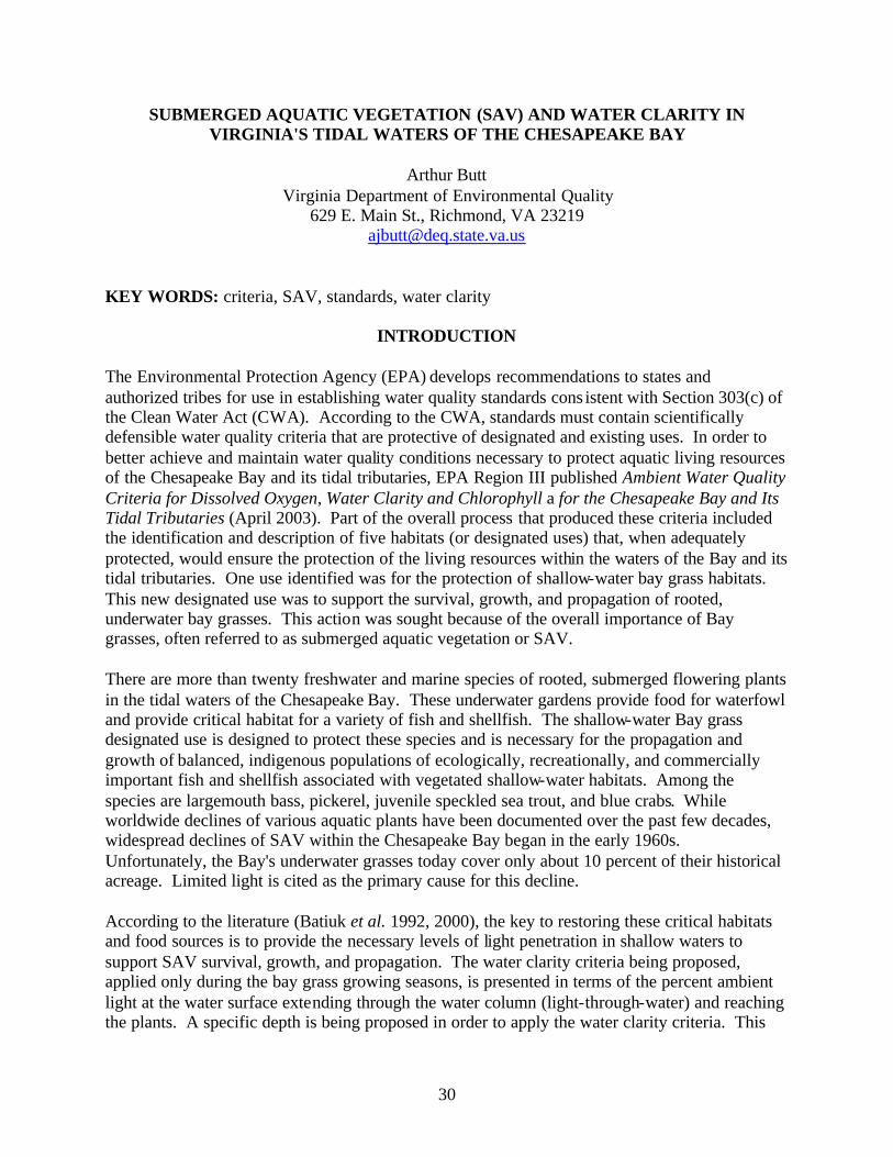
SUBMERGED AQUATIC VEGETATION (SAV) AND WATER CLARITY IN VIRGINIA'S TIDAL WATERS OF THE CHESAPEAKE BAY

Arthur Butt

Virginia Department of Environmental Quality 629 E. Main St., Richmond, VA 23219

ajbutt@deq.state.va.us

KEY WORDS: criteria, SAV, standards, water clarity

INTRODUCTION The Environmental Protection Agency (EPA) develops recommendations to states and authorized tribes for use in establishing water quality standards cons istent with Section 303(c) of the Clean Water Act (CWA). According to the CWA, standards must contain scientifically defensible water quality criteria that are protective of designated and existing uses. In order to better achieve and maintain water quality conditions necessary to protect aquatic living resources of the Chesapeake Bay and its tidal tributaries, EPA Region III published Ambient Water Quality Criteria for Dissolved Oxygen, Water Clarity and Chlorophyll a for the Chesapeake Bay and Its Tidal Tributaries (April 2003). Part of the overall process that produced these criteria included the identification and description of five habitats (or designated uses) that, when adequately protected, would ensure the protection of the living resources within the waters of the Bay and its tidal tributaries. One use identified was for the protection of shallow-water bay grass habitats. This new designated use was to support the survival, growth, and propagation of rooted, underwater bay grasses. This action was sought because of the overall importance of Bay grasses, often referred to as submerged aquatic vegetation or SAV. There are more than twenty freshwater and marine species of rooted, submerged flowering plants in the tidal waters of the Chesapeake Bay. These underwater gardens provide food for waterfowl and provide critical habitat for a variety of fish and shellfish. The shallow-water Bay grass designated use is designed to protect these species and is necessary for the propagation and growth of balanced, indigenous populations of ecologically, recreationally, and commercially important fish and shellfish associated with vegetated shallow-water habitats. Among the species are largemouth bass, pickerel, juvenile speckled sea trout, and blue crabs. While worldwide declines of various aquatic plants have been documented over the past few decades, widespread declines of SAV within the Chesapeake Bay began in the early 1960s. Unfortunately, the Bay's underwater grasses today cover only about 10 percent of their historical acreage. Limited light is cited as the primary cause for this decline. According to the literature (Batiuk et al. 1992, 2000), the key to restoring these critical habitats and food sources is to provide the necessary levels of light penetration in shallow waters to support SAV survival, growth, and propagation. The water clarity criteria being proposed, applied only during the bay grass growing seasons, is presented in terms of the percent ambient light at the water surface extending through the water column (light-through-water) and reaching the plants. A specific depth is being proposed in order to apply the water clarity criteria. This

31

paper reviews SAV acreage in Virginia's tidal waters and characterizes water clarity conditions based on the available data from the Chesapeake Bay Monitoring Program. Several conclusions are made regarding the use of water clarity criteria, and suggestions for enhanced monitoring to better measure water clarity are provided.

METHODS SAV acreage in Virginia's tidal waters was based on the historical records interpreted from aerial photographs. The records available included photographs from the 1930s and 1950s (i.e., historical) as well as the annual bay-wide aerial survey data from 1978-2000. From these photos, the acreage of SAV within three depth intervals was calculated for every Bay segment. The depth intervals were 0-0.5 m, 0.5-1.0 m, and 1.0 - 2.0 m. Thus, each segment had three "segment-depth intervals." Acreage within each segment-depth was an estimate of the potential SAV habitat in that segment-depth interval. A new method was adopted that used the observed single best year (SBY) of SAV coverage for each whole segment (i.e., not the single best year by segment-depth). A set of decision rules was developed based on the observed SBY of SAV coverage for each whole segment. Using each segment's SBY, the percentage of available habitat at each segment-depth interval where SAV occurred in that SBY was calculated. The light attenuation coefficient (Kd) habitat requirement reflects the minimum water column light attenuation level at which SAV can survive and grow. Batiuk et al. (1992) established light-through-water requirements by salinity regime for the restoration of SAV in the Chesapeake Bay. Light attenuation coefficients are calculated based on Beer's Law Iz = Io -KdZ, where Io is light (photosynthetically active radiation -PAR) measured just below the surface and Iz is light measured at some depth. Using the relationship:

Percent light-through-water = 100 * exp (-Kd * Z): where Z = depth in the water column or the depth based on the water clarity criteria application depth. The minimum seasonal percent light requirements were determined to be 13 percent in tidal- fresh and oligohaline environments and 22 percent in meso- and polyhaline environments (Batiuk et al. 1992, 2000). The application depths for Virginia tidal waters were 0.5 m in the tidal- fresh and oligohaline and 1.0 m in the meso- and polyhaline regions.

RESULTS A summary of SAV acreage for Virginia's tidal waters based on the historical records interpreted from aerial photographs is provided (Table 1). The higher salinity regions of the lower estuary tend to support the highest abundance SAV acreage. Of Virginia's three major tributaries, the York River (YRKPH), including Mobjack Bay (MOBPH), showed a SBY with over 12,000 acres. The Rappahannock River (RPPMH), including the Corrotoman and Piankatank rivers, recorded a SBY of over 8,000 acres, while the lower James (JMSMH and JMSPH) had only about 1,000 acres (SBY). The tidal fresh sections of the upper James (JMSTF) historically had 1,600 acres of SAV (SBY). The Mattaponi (MPNTF) and Pamunkey (PMKTF) (York River) had less than 200 acres (SBY), and the upper Rappahannock (RPPTF) had just 20 acres of SAV

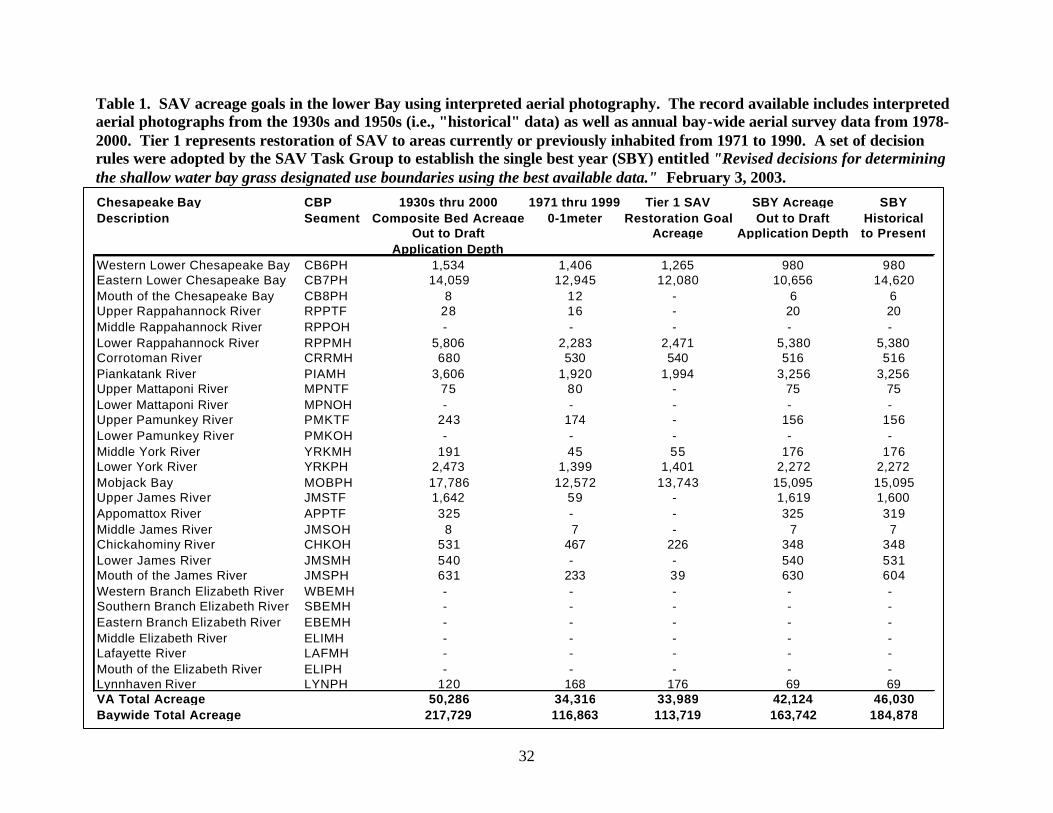
32

Table 1. SAV acreage goals in the lower Bay using interpreted aerial photography. The record available includes interpreted aerial photographs from the 1930s and 1950s (i.e., "historical" data) as well as annual bay-wide aerial survey data from 1978-2000. Tier 1 represents restoration of SAV to areas currently or previously inhabited from 1971 to 1990. A set of decision rules were adopted by the SAV Task Group to establish the single best year (SBY) entitled "Revised decisions for determining the shallow water bay grass designated use boundaries using the best available data." February 3, 2003. Chesapeake Bay CBP 1930s thru 2000 1971 thru 1999 Tier 1 SAV SBY Acreage SBYDescription Segment Composite Bed Acreage 0-1meter Restoration Goal Out to Draft Historical

Out to Draft Acreage Application Depth to PresentApplication Depth

Western Lower Chesapeake Bay CB6PH 1,534 1,406 1,265 980 980Eastern Lower Chesapeake Bay CB7PH 14,059 12,945 12,080 10,656 14,620Mouth of the Chesapeake Bay CB8PH 8 12 - 6 6Upper Rappahannock River RPPTF 28 16 - 20 20Middle Rappahannock River RPPOH - - - - - Lower Rappahannock River RPPMH 5,806 2,283 2,471 5,380 5,380Corrotoman River CRRMH 680 530 540 516 516Piankatank River PIAMH 3,606 1,920 1,994 3,256 3,256Upper Mattaponi River MPNTF 75 80 - 75 75Lower Mattaponi River MPNOH - - - - - Upper Pamunkey River PMKTF 243 174 - 156 156Lower Pamunkey River PMKOH - - - - - Middle York River YRKMH 191 45 55 176 176Lower York River YRKPH 2,473 1,399 1,401 2,272 2,272Mobjack Bay MOBPH 17,786 12,572 13,743 15,095 15,095Upper James River JMSTF 1,642 59 - 1,619 1,600Appomattox River APPTF 325 - - 325 319Middle James River JMSOH 8 7 - 7 7Chickahominy River CHKOH 531 467 226 348 348Lower James River JMSMH 540 - - 540 531Mouth of the James River JMSPH 631 233 39 630 604Western Branch Elizabeth River WBEMH - - - - - Southern Branch Elizabeth River SBEMH - - - - - Eastern Branch Elizabeth River EBEMH - - - - - Middle Elizabeth River ELIMH - - - - - Lafayette River LAFMH - - - - - Mouth of the Elizabeth River ELIPH - - - - - Lynnhaven River LYNPH 120 168 176 69 69VA Total Acreage 50,286 34,316 33,989 42,124 46,030Baywide Total Acreage 217,729 116,863 113,719 163,742 184,878

33

in a SBY. Among tidal waters, the middle sections of each tributary host the least acreage. No SAV were observed in the Rappahannock River (RPPOH). Limited amounts (SBY less than 200 acres) were seen in the lower Mattaponi (MPNOH), Pamunkey (PMKOH), and middle York (YRKMH). The middle James (JMSOH) reported only 7 acres for a SBY, and none was observed in the Elizabeth or Lafayette rivers. Specific management goals for each Bay segment are also provided in Table 1. The original Chesapeake Bay Program SAV restoration goal was 114,000 acres representing around 34,000 acres in Virginia waters. This goal, formally adopted by the signatories to the Bay Program Partnership in 1992, was to achieve those acres by 2003. This acreage closely matches the observed acreage of nearly 117,000 acres based on 1971 through 1999 observations out to an attainment depth of 1 meter. The SBY acreage out to the draft application depth yields an estimate SAV acreage approaching 164,000 acres. A new SAV goal of 185,000 acres was adopted by the Bay Agreement signatories this year. This new SAV goal includes acreage targets for each Chesapeake Bay Program segment. The largest SAV acreage estimates of around 218,000 acres stem from composite SAV bed acreage out to the application depth based on records from the 1930s through 2000. A Baywide SAV goal of 185,000 acres translates to about 46,000 acres in Virginia's tidal waters. Light attenuation (as measured by Kd) varied both temporally and spatially during the SAV growing season (April through October). Light was most limiting to SAV during the spring (April and May), with most light available through the water column in August (Figure 1). Light was most limiting in the tidal York River and least in the Potomac River (Figure 2). All the basins displayed greatest light attenuation around the estuarine turbidity maximum (RET).

Figure 1. Light attenuation by month for lower tributaries (1994-2001). While all of these measurements were taken in the mid-channel regions of each tributary, a limited record of near-shore data was collected in 1994. The best shallow and mid-channel comparisons were in the tidal fresh (TF) where the near-shore Kd values were only 8% above those in the mid-channel (Table 2). The transitional zone (RET) of the estuary characterized by the turbidity maximum was highly divergent with the shallows showing light attenuation of 12% to 48% above mid-channel values. The lower estuary (LE) shallows were consistently higher at 27% above mid-channel values. While only one station (LE4.2) failed the minimum

0

2

4

6

8

1 0

1 2

1 4

A p r i l M a y J u n e J u l y A u g S e p t O c t

B a s i n

K d

J a m e s Y o r k R a p p P o t o m a c

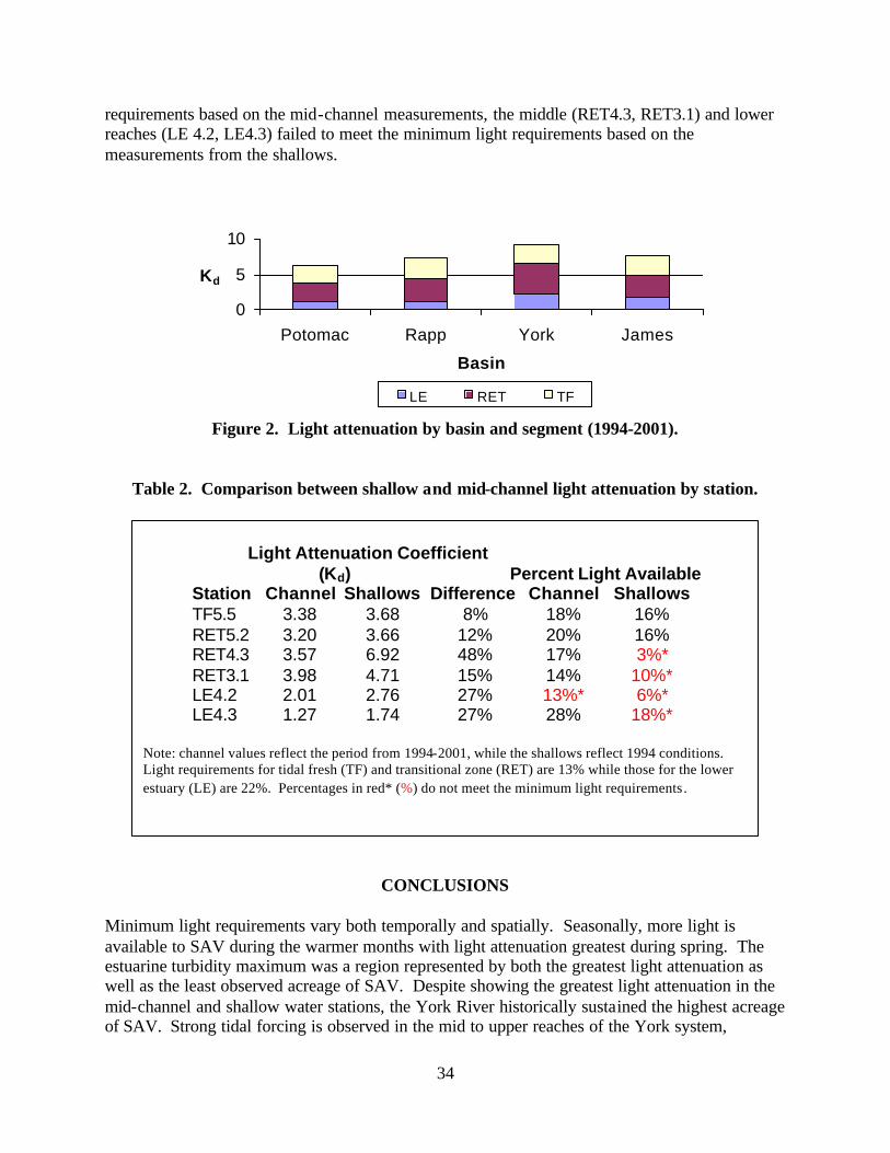
34

requirements based on the mid-channel measurements, the middle (RET4.3, RET3.1) and lower reaches (LE 4.2, LE4.3) failed to meet the minimum light requirements based on the measurements from the shallows.

Figure 2. Light attenuation by basin and segment (1994-2001).

Table 2. Comparison between shallow and mid-channel light attenuation by station.

CONCLUSIONS Minimum light requirements vary both temporally and spatially. Seasonally, more light is available to SAV during the warmer months with light attenuation greatest during spring. The estuarine turbidity maximum was a region represented by both the greatest light attenuation as well as the least observed acreage of SAV. Despite showing the greatest light attenuation in the mid-channel and shallow water stations, the York River historically sustained the highest acreage of SAV. Strong tidal forcing is observed in the mid to upper reaches of the York system,

0

5

10

Potomac Rapp York James

Basin

Kd

LE RET TF

Light Attenuation Coefficient

(Kd) Percent Light Available Station Channel Shallows Difference Channel Shallows TF5.5 3.38 3.68 8% 18% 16% RET5.2 3.20 3.66 12% 20% 16% RET4.3 3.57 6.92 48% 17% 3%* RET3.1 3.98 4.71 15% 14% 10%* LE4.2 2.01 2.76 27% 13%* 6%* LE4.3 1.27 1.74 27% 28% 18%*

Note: channel values reflect the period from 1994-2001, while the shallows reflect 1994 conditions. Light requirements for tidal fresh (TF) and transitional zone (RET) are 13% while those for the lower estuary (LE) are 22%. Percentages in red* (%) do not meet the minimum light requirements.

35

contributing to a highly unstable and variable bottom environment. As a result, light attenuation in the mid-channel and shallow water stations were observed. More stable conditions seem to exist in the lower York where historical SAV acreage is high. Adoption of a water quality standard based entirely on the minimum light requirement(s) for SAV may not be justified. An alternative would be to adopt a biological standard based on a set of predetermined SAV acreage goals. For example, the number of SAV acres would be used to first measure attainment. If the measured number of acres meets the criteria, then the adopted standard for that segment or basin is in attainment. If the segment fails to meet the established standard, then an alternative approach is needed. Rather than adopt standards based on a biological metric (acreage) plus some water clarity metric based on a predetermined application depth for each segment and basin, an established SAV acreage of existing and potential habitat could be used. For example, suppose a segment or basin has a goal of 1,000 acres of SAV. Surveys determine there are only 500 acres of SAV present and an additional 500 acres (or some predetermined ratio) of potential shallow water habitat. If both the acreage plus the predetermined potential habitat meet the minimum light requirement, the segment or basin would be in attainment. The decision to use mid-channel data to characterize shallow habitat conditions should be done on a site-by-site basis. Because SAV beds are not distributed uniformly, a tiered or prioritized monitoring profile could be developed. Since the turbidity maximum is a region with naturally high light attenuation with limited SAV acreage, ambient monitoring in and around this area could be avoided. There are wide variations in the results between shallow and mid-channel data. Previous studies have determined that it is possible to determine a distance from a specific mid-channel station for which it may be appropriate to use the mid-channel monitoring results to characterize the shallow water environment (Batiuk et al. 2000). Although light is the primary factor controlling the distribution of SAV in the Bay, other environmental factors may limit their growth despite the presence of adequate light requirements (Livingston et al. 1998). Such factors include the availability of propagules or seeds, salinity, temperature, water depth, tidal range, grazers, suitable sediment or substrate quality, nutrients in the sediments or water, wave action, current velocity, and chemical contaminants (Koch 2001). While some of these factors have a direct influence on SAV growth and survival, others inhibit the interaction of SAV and light or the surrounding habitat and thereby restrict SAV survival. Therefore, minimum light requirements may be site specific depending on other limiting factors. There are special problems when trying to correlate sediment loadings to water clarity conditions and possible attainment in the tributaries. The major sources of fine-grained sediments in the estuary are supplied from both external and internal sources (Chesapeake Bay Program 2003). Three major externa l sources include the above fall line watersheds, below fall line watersheds, and oceanic inputs. While the tidal freshwaters are dominated by fall line loadings, the lower tributaries are influenced by both below fall line sediments and oceanic inputs. Estimates indicate that the oceanic source is at least equal to or greater than below fall line sources. Data gathered from the Goodwin Islands in the lower York River concluded that local resuspension of bottom sediment was limited and that much of the material was brought to the site by advective processes (Boon 1996). Therefore, much of the water clarity at the mouths of the James and

36

York rivers (and to a lesser degree the Rappahannock) could be attributed to natural or background conditions. For such conditions, mid-channel data could be used to establish a natural background condition from which near-shore data could be compared.

ACKNOWLEDGMENTS

The author wishes to thank Cindy Johnson for assistance with monitoring data and John Kennedy for his critical review of the manuscript.

REFERENCES Batiuk, R., R. Orth, K. Moore, J.C. Stevenson, W. Dennison, L. Staver, V. Carter, N. Rybici, R. Hickman, S. Kollar and S. Bieber. 1992. Submerged Aquatic Vegetation Habitat Requirements and Restoration Targets: A Technical Synthesis. Chesapeake Bay Program. Annapolis, Md. Batiuk, R., P. Bergstrom, M. Kemp, E. Koch, L. Murry, J. Court Stevenson, R. Bartleson, V. Carter, N. Rybicki, J. Lanwehr, C. Gallegos, L. Karrh, M. Naylor, D. Wilcox, K. Moore, S. Ailstock, M. Teichberg. 2000. Chesapeake Bay Submerged Aquatic Vegetation Water Quality and Habitat-Based Requirements and Restoration Targets: A Second Technical Synthesis. August. Chesapeake Bay Program. Annapolis, Md. Boon, J.D. 1996. Hydrodynamics of Sediment Suspension in the Littoral Zone of the Lower York River - Phase I. Virginia Coastal Resources Management Program/Virginia Department of Environmental Quality, Final Report. Chesapeake Bay Program. 2003. A Summary Report of Sediment Processes in Chesapeake Bay and Watershed. Nutrient Subcommittee Sediment Workgroup, Draft Report. January. Environmental Protection Agency. 2003. Ambient Water Quality Criteria for Dissolved Oxygen, Water Clarity and Chlorophyll a for the Chesapeake Bay and Its Tidal Tributaries . U.S. EPA Region III. http://www.epa.gov/chesapeake/baycriteria/Criteria_Final.pdf (December 10, 2003). Koch, E.W. 2001. Beyond light: Physical, geological and geochemical parameters as possible submersed aquatic vegetation habitat requirements. Estuaries 24: 1-17. Livingston, R. J., S. E. McGlynn and X. Niu. 1998. Factors controlling seagrass growth in a gulf coastal system: water and sediment quality and light. Aquatic Biology 60: 135-159.

37

SYNOPSIS OF OUTCOMES FROM THE FEDERAL INTERAGENCY WORKSHOP ON TURBIDITY AND OTHER SEDIMENT SURROGATES

John R. Gray

U.S. Geological Survey 415 National Center, Reston, VA 20192

jrgray@usgs.gov

G. Douglas Glysson U.S. Geological Survey

412 National Center, Reston, VA 20192

KEY WORDS: turbidity, water clarity, suspended sediment, sediment-surrogate technology

ABSTRACT The goals of the April 30-May 2, 2002, Federal Interagency Subcommittee on Sedimentation Workshop on “Turbidity and Other Sediment Surrogates,” were to (1) propose a technically supportable, unambiguous definition of turbidity, and (2) describe the proper use, capabilities, and limitations of turbidimeters and other instruments for providing reliable surrogate data to characterize selected properties of suspended sediment, and for sediment- flux computations. There is considerable ambiguity in the definition, meter calibration, and measurement of turbidity. Turbidity measurements can be unreliable and relatively inaccurate. A new standard method for measurement of the optical properties of natural water and wastewater is recommended. Standard and reliable procedures are needed for measuring and storing data on water clarity and suspended sediment, and for computing sediment fluxes.

INTRODUCTION

Methodologies for quantifying the clarity or solid-phase content of surface waters that require routine collection and subsequent analysis of water samples are well established (Wilde and Gibs 1998, Edwards and Glysson 1999). However, these traditional methods are increasingly being forsaken in favor of less expensive, potentially safer continuously recording in situ methods for monitoring water clarity and (or) for obtaining surrogate1 data for quantification, including analysis of uncertainty of selected sedimentary characteristics of surface waters. Monitoring turbidity is the most common means for obtaining water-clarity data, and for inferring suspended-sediment concentrations. Other sediment-surrogate measurement techniques, including those based on laser-optical, digital-optical, acoustical, and pressure-differential technologies, are increasingly being used (Gray et al. 2003).

1 As used in this report, a surrogate is an environmental measurement than can be reliably correlated with an in-stream characteristic, such as concentration or particle -size distribution of fluvial sediment. Surrogate data are typically easier, less expensive, and (or) safer to collect than the target variable, and may enable reliable estimates of uncertainty associated with the measurement.

38

The proliferation of instruments for measuring water clarity and the sedimentary properties of water has occurred despite a lack of nationally accepted standards for collection or use of data derived from these techniques. For example, there are currently many designs of “turbidity” meters (turbidimeters) that use different approaches and light sources to determine “turbidity” in situ or in a sample. Some are based on the International Standards Organization standard 7027 (ISO 1999); some are based on the U.S. Environmental Protection Agency Method 180.1 (U.S. Environmental Protection Agency 1999); and some are based on neither of these standards, yet, all derivative data from these methods are reported as “turbidity.” A need for better understanding and standardization of data produced by turbidity meters and other sediment-surrogate technologies was the impetus for holding the Workshop on “Turbidity and Other Sediment Surrogates.” The goals of the Workshop were to:

• Propose a technically supportable, unambiguous definition of turbidity, • Describe the proper use and limitations of instruments to measure turbidity of a stream

and to infer suspended-sediment concentrations from turbidity, and • Identify capabilities and limitations of other instruments and (or) techniques that might be

used to measure concentrations and other selected characteristics of suspended sediment and compute sediment fluxes.

Outcomes from the Workshop, summarized by Gray and Glysson (2003), were derived through results of a pre-Workshop questionnaire completed by representatives from most of the States and some Tribes; through measurements of the turbidity of blind quality-control samples made during the Workshop; and through the deliberations of the following four breakout sessions:

• Definition of Optical Methods for Turbidity and Data Reporting, • Use of Optical Properties to Monitor Turbidity and Suspended-Sediment Concentration, • Computing Suspended-Sediment Records Using Surrogate Measurements, • Other Fluvial-Sediment Surrogates.

The major findings and recommendations from the Workshop are described in the following sections.

MAJOR FINDINGS FROM THE WORKSHOP The order in which the major findings are provided does not imply ranking of the findings.

1. Nature of Turbidity: Turbidity is a crucial property in water-quality regulation, but it is

not a well-defined quantity. Different sensors and standards will produce different results from the same sample. This ambiguity complicates the development of turbidity monitoring programs, regulations based on measured turbidity, and the application of estimates of water clarity and sediment concentrations based on those data.

2. Variance in Turbidity Measurements: A review of standard calibration protocols from

different manufacturers had noted differences of less than 5 percent among the standards.

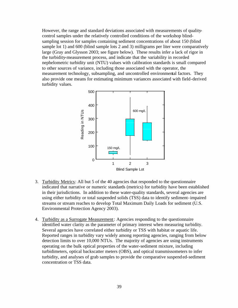
39

However, the range and standard deviations associated with measurements of quality-control samples under the relatively controlled conditions of the workshop blind-sampling session for samples containing sediment concentrations of about 150 (blind sample lot 1) and 600 (blind sample lots 2 and 3) milligrams per liter were comparatively large (Gray and Glysson 2003; see figure below). These results infer a lack of rigor in the turbidity-measurement process, and indicate that the variability in recorded nephelometric turbidity unit (NTU) values with calibration standards is small compared to other sources of variance, including those associated with the operator, the measurement technology, subsampling, and uncontrolled environmental factors. They also provide one means for estimating minimum variances associated with field-derived turbidity values.

1 2 3

Blind Sample Lot

0

100

200

300

400

500

Rea

ding

in N

TU

s

3. Turbidity Metrics: All but 5 of the 40 agencies that responded to the questionnaire

indicated that narrative or numeric standards (metrics) for turbidity have been established in their jurisdictions. In addition to these water-quality standards, several agencies are using either turbidity or total suspended solids (TSS) data to identify sediment- impaired streams or stream reaches to develop Total Maximum Daily Loads for sediment (U.S. Environmental Protection Agency 2003).

4. Turbidity as a Surrogate Measurement : Agencies responding to the questionnaire

identified water clarity as the parameter of primary interest when measuring turbidity. Several agencies have correlated either turbidity or TSS with habitat or aquatic life. Reported ranges in turbidity vary widely among reporting agencies, ranging from below detection limits to over 10,000 NTUs. The majority of agencies are using instruments operating on the bulk optical properties of the water-sediment mixture, including turbidimeters, optical backscatter meters (OBS), and optical transmissometers to infer turbidity, and analyses of grab samples to provide the comparative suspended-sediment concentration or TSS data.

600 mg/L

150 mg/L

40

5. Turbidity Calibration Standard and Method: The majority of States and Tribes who responded to the questionnaire and that measure turbidity use formazin as a calibration standard and U.S. Environmental Protection Agency Method 180.1 for analysis.

6. Turbidity Data Storage: The majority of the agencies responding to the questionnaire use

Oracle, STORET, or a local database or spreadsheet for data storage and analysis. Data currently are stored under a parameter code designated as “turbidity” and no distinction is made between data collected using different equipment technologies or collection procedures. As illustrated by the blind sample test, considerable variance among measurements of the same sample can exist. Because of this variance, the existing data will probably not be comparable with data in other data sets and possibly not compatible within a given data set.

7. Proliferation of Other Sediment-Surrogate Technologies: A number of surrogate

technologies other than turbidity are being used to infer suspended-sediment concentrations and other characteristics of fluvial sediment. These data suffer from many of the same drawbacks as those associated with turbidity, including the lack of reliable standards for in situ calibration.

PRINCIPAL WORKSHOP RECOMMENDATIONS TO THE FEDERAL

INTERAGENCY SUBCOMMITTEE ON SEDIMENTATION The order in which the principal recommendations are provide does not imply ranking.

1. Turbidity Definition: Adopt the current definition of turbid ity for natural water and wastewater, contained in ASTM Standard Test Method for Turbidity in Water, D 1889-00 (ASTM International 2002), as follows: Turbidity—an expression of the optical properties of a sample that causes light rays to be scattered and absorbed rather than transmitted in straight lines through a sample. (Turbidity of water is caused by the presence of suspended and dissolved matter such as clay, silt, finely divided organic matter, plankton, other microscopic organisms, organic acids, and dyes.)

2. New Turbidity Standard Method: Adopt a new standard method for the measurement of

the optical properties of natural water and wastewater. The method should include a hierarchical decision tree for selection of an instrument for a specific application. The method should specify that the different instrument types and models will yield different turbidity results and generally should not be expected to be equivalent. Existing water-quality monitoring guidelines, with consideration for instrument manufacturer protocols, should be updated to reflect the new standard method.

3. Storage of Turbidity Data: Until a uniform industry standard is developed for the

measurement and storage of the optical properties of water, consider storing the derivative data on the basis of instrument manufacturer, an instrument identifier, and sensor mode, or use another method that captures most or all of the specific information that may enable eventual adjustment of these data. Data descriptors for internal and external use with a detailed description of the turbidity methodology should be included

41

in the database. A set of proposed turbidity reporting units to differentiate between various instruments and methodologies should be developed (data reporting should consider and include incident light wavelength, orientation and number of detectors, instrument manufacturer, model number, calibration measurement documentation, reporting of variability, and other relevant factors.)

4. Retrospective Turbidity Comparisons : Quantify instrument differences to enable valid

comparisons that may be required for retrospective data mining for comparison of data collected by new and historical techniques. Document the percentage difference in data derived by historical and newer methods, and include references for published reports that compare turbidity data collected with different instruments and (or) methods.

5. Technology Transfer and Communication: Increase technology transfer between groups

and individuals with interests in turbidity and other sediment-surrogate technologies. A steering committee should be formed that includes a coordinator and topical expert advisers on turbidity and on other sediment-surrogate technologies. Resources associated with the steering committee may include publication of a newsletter, creating and maintaining a web-based compilation of information, supporting user groups and on- line help, documenting methods, transferring industrial technology to the environmental field, and otherwise providing guidance to the Subcommittee on Sedimentation.

6. Stakeholder and Peer Review: Keep the public and users of turbidity and other sediment-

surrogate data informed of the issues involved in producing these data, including assumptions, limitations, methods, and applicability.

7. Testing and Development Program for Instruments and Methods: Develop a program to

foster research, testing, and evaluation of instruments and methods for measuring, monitoring, and analyzing water clarity and selected characteristics of fluvial sediment by cost-effective, safe, and quantifiably accurate means. Technically supportable and widely available standard guidelines for sensor deployment, calibration, and data processing (including real-time data) are needed. Acceptance criteria for data from given parameters, such as suspended-sediment concentration, should be developed, endorsed by the Subcommittee on Sedimentation, and widely advertised to encourage methods and instrumentation development.

8. Collection and Computation of Sediment-Surrogate Records: Develop standardized

procedures for the collection of sediment-surrogate data. These standardized procedures should include protocols for instrument calibration and criteria for acceptance of the derivative sediment data. A standard procedure for computation of sediment-discharge records should be developed for all sediment-surrogate records utilizing the fullest set of data.

9. Technical Needs for Turbidity Measurements: The agencies responding to the

questionnaire identified several technical needs related to turbidity including: a. Improve the understanding of the relation between turbidity, total suspended solids,

suspended-sediment concentration, channel stability, and biological impairment.

42

b. Establish reference conditions for fluvial sediment and a means of measuring significant departure from the reference conditions.

c. Develop a consistent data-collection protocol and less expensive probes that can be rapidly deployed and are stable in the field.

d. Obtain more long-term stream discharge, suspended-sediment, bedload, and bed-material data.

ACKNOWLEDGMENTS

The authors wish to thank the Federal Interagency Subcommittee on Sedimentation for sponsoring the April 30-May 2, 2002, “Turbidity and Other Sediment Surrogates Workshop,” on which this synopsis is based. We also wish to thank Dominic Roques, Central Coast Regional Water Quality Control Board, San Luis Obispo, California; and Scott A. Wright, U.S. Geological Survey, Sacramento, California, for their excellent reviews of this manuscript.

REFERENCES ASTM International. 2002. Standards on Disc. Section Eleven, Water and Environmental Technology. Volume 11.02. Edwards, T.K. and G.D. Glysson. 1999. Field methods for measurement of fluvial sediment. In: U.S. Geological Survey Techniques of Water-Resources Investigations. Book 3, Chapter 2. 89 pp. http://water.usgs.gov/osw/techniques/Edwards-TWRI.pdf (June 13, 2003). Gray, J.R. and G.D. Glysson. 2003. Proceedings of the federal interagency workshop on turbidity and other sediment surrogates. In: U.S. Geological Survey Circular 1250, in press. http://water.usgs.gov/osw/techniques/turbidity.html (June 30, 2003). Gray, J.R., E. Patiño, P.P. Rasmussen, M.C. Larsen, T.S. Melis, D.J. Topping, and C.F. Alamo. 2003. Evaluation of sediment surrogate technologies for computation of suspended-sediment transport. In: Proceedings of the 1st International Yellow River Forum on River Basin Management, Yellow River Conservancy Commission. 10 pp. http://water.usgs.gov/osw/techniques/yrcc_surrogates.pdf (June 2, 2003). International Organiza tion for Standardization. 1999. Water quality—Determination of turbidity. In: Geneva, Switzerland, International Organization for Standardization, ISO 7027. 10 pp. U.S. Environmental Protection Agency. 1999. Guidance Manual for Compliance with the Interim Enhanced Surface Water Treatment Rule—Turbidity Provisions. Office of Water, 815-R-99-010, variously paged. http://www.epa.gov/safewater/mdbp/pdf/turbidity (May 21, 2003). U.S. Environmental Protection Agency. 2003. Total maximum daily loads. http://www.epa.gov/ebtpages/watewaterptotalmaximumdailyloadstmdls.html (May 22, 2003).

43

Wilde, F.C., and J. Gibs. 1998. Turbidity: National field manual for the collection of water-quality data. In: Techniques of Water-Resources Investigations. Book 9, Chapter 6.7. 30 pp. http://water.usgs.gov/owq/FieldManual/Chapter6/6.7_contents.html (May 12, 2003).

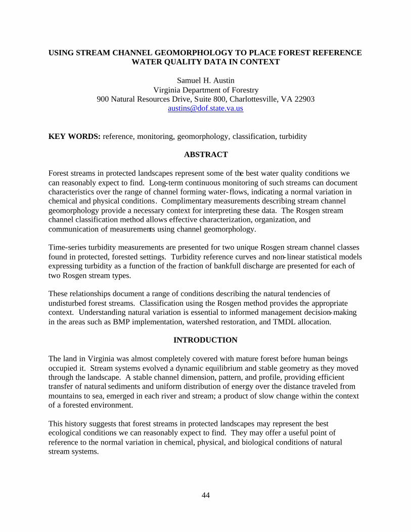
44

USING STREAM CHANNEL GEOMORPHOLOGY TO PLACE FOREST REFERENCE WATER QUALITY DATA IN CONTEXT

Samuel H. Austin

Virginia Department of Forestry 900 Natural Resources Drive, Suite 800, Charlottesville, VA 22903

austins@dof.state.va.us

KEY WORDS: reference, monitoring, geomorphology, classification, turbidity

ABSTRACT Forest streams in protected landscapes represent some of the best water quality conditions we can reasonably expect to find. Long-term continuous monitoring of such streams can document characteristics over the range of channel forming water- flows, indicating a normal variation in chemical and physical conditions. Complimentary measurements describing stream channel geomorphology provide a necessary context for interpreting these data. The Rosgen stream channel classification method allows effective characterization, organization, and communication of measurements using channel geomorphology. Time-series turbidity measurements are presented for two unique Rosgen stream channel classes found in protected, forested settings. Turbidity reference curves and non- linear statistical models expressing turbidity as a function of the fraction of bankfull discharge are presented for each of two Rosgen stream types. These relationships document a range of conditions describing the natural tendencies of undisturbed forest streams. Classification using the Rosgen method provides the appropriate context. Understanding natural variation is essential to informed management decision-making in the areas such as BMP implementation, watershed restoration, and TMDL allocation.

INTRODUCTION The land in Virginia was almost completely covered with mature forest before human beings occupied it. Stream systems evolved a dynamic equilibrium and stable geometry as they moved through the landscape. A stable channel dimension, pattern, and profile, providing efficient transfer of natural sediments and uniform distribution of energy over the distance traveled from mountains to sea, emerged in each river and stream; a product of slow change within the context of a forested environment. This history suggests that forest streams in protected landscapes may represent the best ecological conditions we can reasonably expect to find. They may offer a useful point of reference to the normal variation in chemical, physical, and biological conditions of natural stream systems.

45

The Virginia Department of Forestry is collecting data that describe these natural, forested stream systems, and is organizing them within the useful context of the Rosgen stream classification system (Rosgen 1994). The idea is to identify the natural chemical, physical, and biological reference condition, over the range of water discharge rates, organized within each of the seven Rosgen stream types in Virginia. The data presented here represent one piece of this ongoing characterization.

METHODS The Rosgen Stream Classification System identifies seven major stream types labeled A through G. Using stream bed particle size distribution, each category is further refined into six sub-classes from 1 (bedrock) to 6 (silt/clay). The system exploits the fact that streams tend to organize themselves around the most likely combination of variables based on physical and chemical laws. This tendency to seek a dynamic equilibrium reflecting landscape conditions in a watershed lends itself nicely to classification. Forested reference streams in protected landscapes are identified, surveyed, and classified using the Rosgen method. For each Rosgen stream type, a reference reach is identified, and permanent surveying stations are established. In situ equipment is installed to characterize reference reach geomorphology, hydraulic geometry, and hydraulic regime. Data are collected to describe the following parameters: Geomorphology: - Stream channel dimension, pattern, and profile.

- Streambed particle size distribution. Hydraulic Geometry: - Change in channel width as a function of water discharge.

- Change in mean channel depth as a function of water discharge. - Change in mean water velocity as a function of water discharge.

Hydrologic Regime: - Rate of water discharge. - Quantity of water discharge. - Water turbidity. - Suspended sediment load. - Water temperature. - Conductivity. - Dissolved oxygen.

- pH. The time-series turbidity measurements presented here are collected continuously at 30-minute intervals using a YSI 6026 wiped turbidity sensor mounted on a YSI 6920 sonde. These time-stamped measurements are matched to simultaneously collected stream stage data, which are used to compute stream water discharge using a separately developed stage-discharge equation. Turbidity data expressed in nephelometric turbidity units (NTU) are plotted against the fraction of bankfull water discharge. Non- linear regression is used to determine a line of best fit and equations predicting turbidity as a function of the fraction of bankfull discharge.

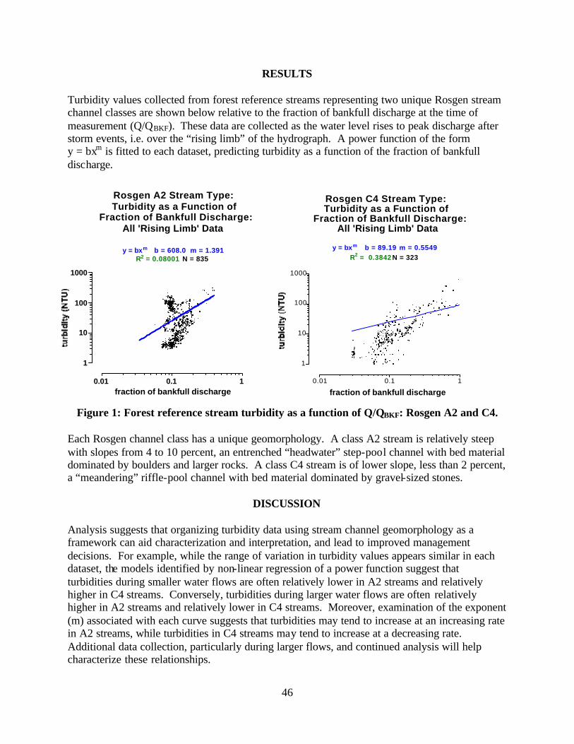
46

RESULTS Turbidity values collected from forest reference streams representing two unique Rosgen stream channel classes are shown below relative to the fraction of bankfull discharge at the time of measurement (Q/QBKF). These data are collected as the water level rises to peak discharge after storm events, i.e. over the “rising limb” of the hydrograph. A power function of the form y = bxm is fitted to each dataset, predicting turbidity as a function of the fraction of bankfull discharge.

Figure 1: Forest reference stream turbidity as a function of Q/QBKF: Rosgen A2 and C4. Each Rosgen channel class has a unique geomorphology. A class A2 stream is relatively steep with slopes from 4 to 10 percent, an entrenched “headwater” step-pool channel with bed material dominated by boulders and larger rocks. A class C4 stream is of lower slope, less than 2 percent, a “meandering” riffle-pool channel with bed material dominated by gravel-sized stones.

DISCUSSION Analysis suggests that organizing turbidity data using stream channel geomorphology as a framework can aid characterization and interpretation, and lead to improved management decisions. For example, while the range of variation in turbidity values appears similar in each dataset, the models identified by non-linear regression of a power function suggest that turbidities during smaller water flows are often relatively lower in A2 streams and relatively higher in C4 streams. Conversely, turbidities during larger water flows are often relatively higher in A2 streams and relatively lower in C4 streams. Moreover, examination of the exponent (m) associated with each curve suggests that turbidities may tend to increase at an increasing rate in A2 streams, while turbidities in C4 streams may tend to increase at a decreasing rate. Additional data collection, particularly during larger flows, and continued analysis will help characterize these relationships.

Rosgen C4 Stream Type:Turbidity as a Function of

Fraction of Bankfull Discharge: All 'Rising Limb' Data

y = bxm b = 89.19 m = 0.5549R2 = 0.3842 N = 323

0.01 0.1 1

1

10

100

1000

fraction of bankfull discharge

Rosgen A2 Stream Type:Turbidity as a Function of

Fraction of Bankfull Discharge:All 'Rising Limb' Data

y = bxm b = 608.0 m = 1.391R2 = 0.08001 N = 835

0.01 0.1 1

1

10

100

1000

fraction of bankfull discharge

47

Forest reference streams are streams in their natural state. They provide a benchmark describing water parameters within their normal range of values. Monitoring these streams is essential to understanding the normal, natural range of stream water conditions. An understanding of and reference to the natural condition is an essential part of a well-developed resource management plan or policy decision. As the need for improved natural resource management intensifies, the need for and application of this type of information becomes more important. Areas of potential application include planning, watershed management decision-making, best management practice (BMP) implementation, watershed restoration, and total maximum daily load (TMDL) allocation.

REFERENCES

Austin, Samuel H. 1999. Riparian Forest Handbook 1. Virginia Department of Forestry. Charlottesville, Va. Dunne, Thomas, and Luna B. Leopold. 1978. Water in Environmental Planning. W.H. Freeman and Company. New York, N.Y. Leopold, Luna B. 1997. Water, Rivers and Creeks. University Science Books. Sausalito, Calif. Leopold, Luna B. 1994. A View of the River. Harvard University Press. Cambridge, Mass. Leopold, Luna B., M. Gordon Wolman, and John P. Miller. 1962. Fluvial Processes in Geomorphology. Dover Publications, Inc. Mineola, N.Y. Rosgen, Dave. 1996. Applied River Morphology. Wildland Hydrology. Pagosa Springs, Colo.

48

NATURAL EROSION RATES FOR RIPARIAN BUFFERS IN THE PIEDMONT OF VIRGINIA

Amy C. Walker Easterbrook, W. M. Aust, C. A. Dolloff, and P. D. Keyser

Department of Forestry, Virginia Tech 228 Cheatham Hall (0324), Blacksburg, VA 24061

amwalker@vt.edu KEY WORDS: natural erosion, USLE, riparian buffer

INTRODUCTION Instream sediments are one of the most common pollutants for streams in the United States. Sediments can naturally occur at levels not adequate for federal or state water quality standards (Fowler and Heady 1981). Natural erosion is a factor that is often forgotten when considering water quality (Lynch and Corbett 1990). Site stability varies with climate, season, topography, watershed size, geology, and soils (Blackburn et al. 1990, Endreny 2002). Some sites will remain stable after a treatment or disturbance while others will erode severely after minimal impact. Sedimentation and nutrient loading can occur on some sites simply because of naturally erodable soils, thus causing natural variability in stream water quality parameters (Vowell 2000, Endreny 2002). Erosion in undisturbed forests usually originates from the stream banks or channel, and/or can be caused by large, intense rainfall events (Blackburn et al. 1990).

The establishment of benchmark rates (rates of natural erosion) is an important step when trying to manage water quality. Benchmark rates are critical when trying to compare the benefits of different management practices during silvicultural operations, or when trying to determine the amount of pollution caused by silvicultural operations (Fowler and Heady 1981, Novotny 1999). Benchmark rates are also needed in order fo r the Clean Water Act (Sec. 502(19)) and the TMDL process to work correctly. However, very few states have determined natural erosion rates in their different ecoregions, and some have created some water quality standards that are impossible to meet even in undisturbed watersheds (Novotny 1999). In 2001, a project was established to study the effectiveness of riparian buffers for protection of water quality from silvicultural harvesting operations in 18 watersheds encompassing intermittent and ephemeral streams. This paper will discuss a portion of the pre-harvest data. Pre-harvest erosion rates were sampled and analyzed to determine natural erosion rates for a one-year period prior to any silvicultural operations using the Universal Soil Loss Equation (USLE) , sediment rods, and instream sediment pads. The use of firm or trade names does not constitute a recommendation or endorsement by the Virginia Water Resources Research Center.

49

METHODS Site Selection: The project was in the Piedmont Province in and around Buckingham County, Virginia, on 18 watersheds. The sites were predominantly 23-25 year old loblolly pine (Pinus taeda L.) plantations that encompassed the head of an intermittent stream and the majority of its watershed. To aid in analysis, the watersheds were blocked based on soils, acreage, slope, and stream characteristics. Sixteen watersheds were treated, and two watersheds served as controls. Treatments: Various widths and harvest levels were examined in order to effectively study the benefits of the riparian buffers. The widths chosen for this project were a 4.57 m stringer, a 15.24 m riparian buffer with no harvest, a 15.24 m riparian buffer with 50% harvest, a 30.48 m riparian buffer with no harvest as a control, and a 30.48 m riparian buffer with 50% harvest. The controls received a 30.48 m riparian buffer with no harvest. Each block contained one of each prescribed treatment, and the two remaining watersheds were blocked together. Transects were established in the upper, middle, and lower portions of the watershed. Transects were 10 m wide and extended for the width of the prescribed riparian buffer. The widths and harvest levels were based on the larger project, and the data for this report is based on pre-harvest measurements. USLE: In order to develop a greater understanding of the watersheds in the study and how they may react to future management, the Universal Soil Loss Equation (Dissmeyer and Foster 1984) was used to predict erosion potential (A). Use of the Universal Soil Loss Equation (USLE) requires that several variables be measured. Rain gauges were used to collect rainfall data for the R factor. Soil samples were taken to find the particle distribution and organic content for the soil erosivity (K) factor. Then each transect was evaluated for slope length and steepness (LS) and cover and management practices (CP). Recorded Rainfall: Regional rainfall data were collected using tipping bucket rain gauges with a HOBO Event data logger. The rain gauges were set on platforms 1 meter high, and the vegetation was cleared from overhead. The rain gauge buckets were set to tip for every 0.254 mm of rainfall and then recorded by the data logger (Blackburn et al. 1990). The rainfall data from the data loggers were uploaded into a computer and processed to find the Erosivity Index (EI) value (Dissmeyer and Foster 1984, Blackburn et al. 1990). Soil Samples: A soil sample was collected for analysis in the center transect for each watershed. The sample consisted of the top 15 cm of mineral soil and all of the organic layers above. The sample was taken back to the lab and analyzed for organic content and particle distribution (Gee and Or 2002) in order to estimate the soil erodibility (K) factor for the USLE (Dissmeyer and Foster 1984). Sediment Rods: Along the downstream side of each transect, a row of sediment rods was installed at intervals of 2.28 m, 7.62 m, 15.24 m, 30.48 m, and 38.1 m from the center of the stream. This was done on each side of the stream for the two-sided watersheds. The sediment rods were 0.6 m lengths of rebar pounded halfway into the ground. The portion of rod above ground was measured to the nearest millimeter at the mineral soil surface (Hudson 1993).

50

Sediment Stones: Stream sedimentation was measured quarterly in all 3 transects for each watershed. The sediment was trapped by 30.48 x 30.48 x 10.16 cm (12 x 12 x 4 in) “sediment stones.” The sediment stones were garden stepping-stones that were chosen because they provided a fixed surface area, were similar in width to the streams, and had a pebble surface matching the substrate of the stream bottoms (Brooks et al. 1997). To measure the sediment deposition, ten depth readings were taken on each stone. The readings were taken at random points on the stone with a clear ruler to the nearest mm (0.04 in). “Dusting” was recorded instead of the depth readings for stones with a light coating of sediment too shallow to be measured accurately. For analysis a sediment depth of 0.05 mm (0.002 in) was used when a “dusting” was recorded.

RESULTS The USLE had low predicted soil losses for the year; this finding is most likely due to the low amount of bare soil, the thick root mat, and the high onsite storage of the forested sites (Figure 1). The watersheds with higher predicted sediment loss have steep slopes and small floodplains. Watersheds with these characteristics have a high topographic factor (LS) (Dissmeyer and Foster 1984). As expected for mature forests, the blocks had similar erosion rates, and all were relatively low (Blackburn et al. 1990). The erosion measured by the sediment rods was much greater than that predicted by the USLE (Figure 1). These higher rates were probably due to several intense storms that occurred during the drought in 2002. These storms produced up to 10% of the annual erosivity in one day and occurred on four separate occasions. The torrential rain produced by these storms contributed to the soil movement within the riparian buffer (Figure 2), led to flushing of the ephemeral streams, and caused scouring and channel movement in several watersheds. The sediment stones did not trap sediment as anticipated. The estimated erosion rates derived from this method were minuscule, being less than 0.003 tons/ac/yr. The failure of the sediment stones to trap sediment was most likely due to scouring during heavy rain events and the otherwise dry streambeds brought on by drought conditions in the region. Of the three erosion estimates used, the sediment rods were the most effective method. However, the rates derived from this method were high and probably not indicative of normal conditions. The USLE values most likely represented the average rates over long periods of time. Storm-induced erosion and the problem associated with sediment loss measurements were also documented by Riekerk et al. (1979) in a study done on three watersheds in Florida. They found that water quality was dominated by intense precipitation and storm flow. The erosion rates found by this study show the necessity for benchmark values to reflect naturally occurring erosion so that these natural rates are not attributed to land management activities. The results also show that measuring instream sedimentation alone may not be a good indicator of erosion caused by land-use practices. As seen in Figure 2, most of the soil loss occurred within the riparian buffer.

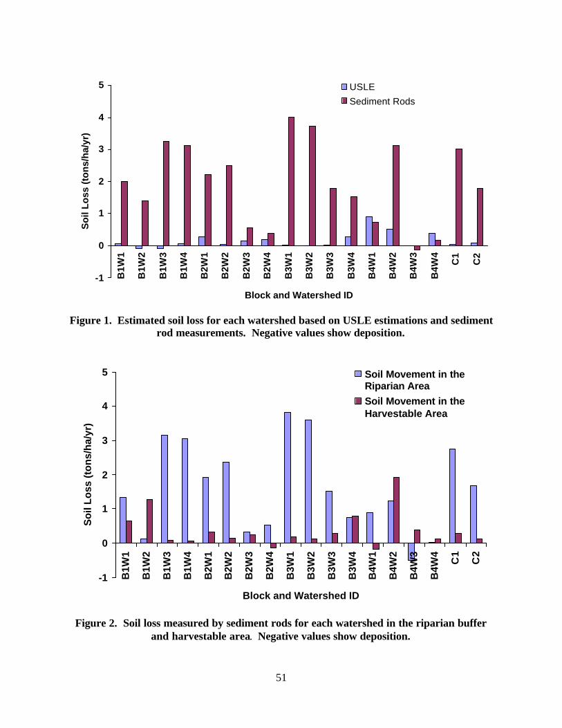
51

-1

0

1

2

3

4

5

B1W

1

B1W

2

B1W

3

B1W

4

B2W

1

B2W

2

B2W

3

B2W

4

B3W

1

B3W

2

B3W

3

B3W

4

B4W

1

B4W

2

B4W

3

B4W

4

C1

C2

Block and Watershed ID

So

il L

oss

(to

ns/

ha/

yr)

USLE

Sediment Rods

Figure 1. Estimated soil loss for each watershed based on USLE estimations and sediment

rod measurements. Negative values show deposition.

-1

0

1

2

3

4

5

B1W

1

B1W

2

B1W

3

B1W

4

B2W

1

B2W

2

B2W

3

B2W

4

B3W

1

B3W

2

B3W

3

B3W

4

B4W

1

B4W

2

B4W

3

B4W

4

C1

C2

Block and Watershed ID

So

il L

oss

(to

ns/

ha/

yr)

Soil Movement in theRiparian AreaSoil Movement in theHarvestable Area

Figure 2. Soil loss measured by sediment rods for each watershed in the riparian buffer and harvestable area. Negative values show deposition.

52

CONCLUSIONS The examined sites had low predicted erosion rates, but higher actual erosion rates, indicating the importance of weather variability. These higher than expected erosion rates and the subsequent trapping of soil by the streamside management zones (SMZ) also indicate the importance of maintaining SMZ even in areas of low expected erosion.

REFERENCES Blackburn, W.H., R.W. Knight, J.C. Wood, and H.A. Pearson. 1990. Stormflow and sediment loss from intensively managed forest watersheds in East Texas. American Water Resources Association. Water Resources Bulletin 26(3): 465-477. Brooks, K.N., P.F. Ffolliott, H.M. Gregersen, and L.F. DeBano. 1997. Hydrology and the Management of Watersheds. 2nd Edition. Iowa State University Press. Ames, Iowa. Dissmeyer, G. E. and G. R. Foster. 1984. A Guide for Predicting Sheet and Rill Erosion on Forest Land. USDA Forest Service Southern Region Technical Publication R8-TP 6. Endreny, T.A. 2002. Forest buffer strips mapping the water quality benefits. Journal of Forestry Jan/Feb (1): 35-40. Fowler, J.M. and E.O. Heady. 1981. Suspended sediment production potential on undisturbed forest land. Journal of Soil and Water Conservation 36(1): 47-50. Gee, G.W. and D. Or. 2002. Particle-size analysis. In: Methods of Soil Analysis Part 4 Physical Methods. J.H. Dane and G.C. Topp (Editors). Soil Science Society of America, Inc., Madison, Wis. pp. 255-289. Hudson, N.W. 1993. Field Measurement of Soil Erosion and Runoff. FAO Soils Bulletin 68. Rome. 139 pp. Lynch, J.A., and E.S. Corbett. 1990. Evaluation of best management practices for controlling nonpoint pollution from silvicultural operations. Water Resources Bulletin 26(1): 41-52. Novotny, V. 1999. Integrating diffuse/nonpoint pollution control and water body restoration into watershed management. Journal of the American Water Resources Association 35(4): 717-727. Riekerk, H., S.A. Jones, L.A. Morris, and D.A. Pratt. 1979. Hydrology and water quality of three lower coastal plain forested watersheds. Soil and Crop Science Society of Florida 38:105-111. Vowell, J.L. 2000. Using stream bioassessment to monitor best management practice effectiveness. Forest Ecology and Management 5273:1-8.

53

U.S. GEOLOGICAL SURVEY SUSPENDED-SEDIMENT SURROGATE RESEARCH, PART I: CALL FOR A SEDIMENT MONITORING INSTRUMENT AND ANALYSIS

RESEARCH PROGRAM

John R. Gray U.S. Geological Survey

415 National Center, Reston, VA 20192 jrgray@usgs.gov

KEY WORDS: fluvial sediment, suspended sediment, monitoring, sediment-surrogate technology

ABSTRACT The number of daily fluvial-sediment data-collection stations operated by the U.S. Geological Survey has declined by almost two-thirds since 1980. This decline has occurred concomitant with a substantial increase in sediment-data needs, and increased availability of potentially useful sediment-surrogate monitoring technologies that lack Federal sanction. The United States would benefit from: (1) a program to foster research, testing, and evaluation of instruments and methods for measuring, monitoring, and analyzing selected characteristics of fluvial sediments in cost-effective, safe, and quantifiably accurate means; (2) use of expert advisors on sediment-surrogate technologies; (3) enhanced communication among those producing or using sediment-surrogate instruments or data; and (4) establishment and promulgation of criteria for evaluating sediment-surrogate technologies and derivative data accuracy.

INTRODUCTION According to the U.S. Environmental Protection Agency (2002), siltation, also referred to as sedimentation, remains one of the most widespread pollutants affecting assessed rivers and streams. In additional to traditional uses of sediment data, such as for design and management of reservoirs and hydraulic structures, information is needed for contaminated sediment management, dam decommissioning and removal, environmental quality, stream restoration, geomorphic classification and assessments, physical-biotic interactions, the global carbon budget, and regulatory requirements of the Clean Water Act, including the U.S. Environmental Protection Agency’s Total Maximum Daily Load Program (U.S. Environmental Protection Agency 2003). The need for reliable, cost-effective, spatially and temporally consistent data to quantify the clarity and sediment content of waters of the United States (U.S.) arguably has never been greater. In spite of the need for more sediment data, there is evidence that the amount of nationally consistent daily sediment data being collected today is but a third of that produced for the U.S. in 1982. This decline is due in part to cost, accuracy, and safety issues (Gray 2002, Gray et al. 2002).

54

Although traditional methodologies that normally require collection and analysis of a physical water sample are well established, these methods are increasingly being forsaken in favor of less expensive, potentially safer continuously recording in situ methods for monitoring water clarity and (or) for obtaining sediment-surrogate data. Turbidity and related bulk-optic measurements are the most common means for obtaining water-clarity data, and for inferring suspended-sediment concentrations. Other sediment surrogate techniques, including those based on laser-optic, digital-optic, acoustic, and pressure-differential technologies, also are being deployed and (or) tested in field and laboratory settings for their applicability toward providing quantifiably reliable information on bedform and bed-material characteristics, and on concentrations, size-distributions and transport rates of suspended sediment and (or) bedload. However, there are no nationally accepted standards for collection, storage, or use of data derived from techniques other than those described by Edwards and Glysson (1999). There is a perceived need for a better understanding and standardization of data produced by these technologies. That perceived need was part of the impetus for holding the Federal Interagency Workshop on Turbidity and Other Sediment Surrogates, April 30-May 2, 2002 (U.S. Geological Survey 2002, Gray and Glysson 2003). The workshop breakout session that focused on suspended-sediment-surrogate technologies other than those based on bulk-optic properties of water proposed four recommendations to the workshop’s sponsor, the Federal Interagency Subcommittee on Sedimentation (Glysson and Gray 1997). The recommendations are summarized as follows: The fluvial-sediment data needs of the U.S. would be well served by:

(1) Forming a program to foster research, testing, and evaluation of instruments and methods for measuring, monitoring, and analyzing selected characteristics of fluvial sediments in cost-effective, safe, and quantifiably accurate means,

(2) Establishing and fostering group(s) of topical expert advisors, composed of private, federal, state, and (or) academia, to advise the Subcommittee on Sedimentation,

(3) Enhancing communication among those producing or using sediment-surrogate instruments or data, and

(4) Establishing and promulgating criteria for suspended-sediment data accuracy. This paper—the first of a 3-part series—addresses the first recommendation shown above by proposing attributes of a Sediment Monitoring Instrument and Analysis Research Program (SMIARP). Activities under the SMIARP would include research on bedload, bed material, and bedforms, in addition to suspended sediment. The other two papers in this 3-part series provide examples of USGS research focusing on optic technologies (Part II) and acoustic and pressure-differential technologies (Part III). SEDIMENT MONITORING INSTRUMENT AND ANALYSIS RESEARCH PROGRAM A SMIARP would focus on instruments and methods for providing quantifiably reliable information on bed-material characteristics, and on concentrations, size distributions and transport rates of sediments in suspension and as bedload by the safest, most cost-effective, and quantifiably accurate means. The following is a vision for a SMIARP as if currently functional.

55

Goal: The goal of the SMIARP is to foster research, testing, and evaluations on instruments and methods for measuring, monitoring, analyzing (including computing and estimating) selected characteristics of fluvial sediments in cost-effective, safe, and quantifiably accurate means. It is desirable that the methods and standards developed through the SMIARP would ultimately be deemed acceptable by standards-setting organizations such as the American Society for Testing and Materials (2003) or the Subcommittee on Sedimentation (Glysson and Gray 1997). Scope: The technical scope of the SMIARP includes research on or related to instruments and methods for remote, in situ, manual and (or) laboratory measurement of selected characteristics of suspended sediment and water clarity, bedload, bed material, and bedforms. The scope includes research on computational and estimating techniques, and the most efficient linkage or usage of instruments, methods, and data-analysis techniques for providing the types and amounts of data needed by the U.S. Functions: The primary functions of the SMIARP are to recommend and (or) provide a formal structure and organization for collaboration; standard data-collection and test protocols; and standard acceptance criteria. The SMIARP also represents a forum or clearinghouse for effective communication between and among public and private entities; and, in some cases, a source of support for organized collaboration on fluvial-sediment research that has a high potential to result in operationally effective tools for providing the sediment data needed by the U.S. Activities: The concept of the SMIARP is evolving and the full range of the program’s potential endeavors is being considered. The following list represents appropriate activities that may be conducted under the auspices of a SMIARP (numbering the activities is for ease in reference and does not imply priority):

1. Develop and publish criteria describing the acceptable documentation, qualification, and reporting of data describing selected characteristics of suspended sediment, bedload, bed material, and bed topography in field and laboratory settings acceptable by standards-setting organizations.

2. Develop and publish quantifiably reliable procedure(s) for testing the precision and bias associated with data obtained by surrogate measurements.

3. Identify instruments, methods, and analytical techniques that show considerable promise for providing surrogate data for fluvial sediment in laboratory and field settings.

4. Test sediment-surrogate instruments in laboratory and (or) in field settings, with the primary goal to describe the capabilities and limits; bias and variance; and requisite ancillary data associated with the instruments.

5. Develop and (or) test analytical techniques for computing or estimating selected characteristics of fluvial sediment, including transport rates, size distributions, and their associated uncertainties.

6. Prepare and disseminate reports that summarize program findings and results. 7. Organize and hold joint briefings, workshops, national meetings, and (or) otherwise

encourage effective communication with program collaborators, the Subcommittee on Sedimentation, its Technical Committee, and the Federal Interagency Sedimentation Project.

56

8. Fund projects, or assist in obtaining project funds to accomplish specific program objectives for which existing resources are inadequate.

9. Evaluate the effectiveness of the SMIARP and refine its mission and (or) functions to optimize its responsiveness to participants.

SUMMARY

In response to expanding needs for fluvial-sediment data concomitant with declines in sediment-data acquisition, formation of a Sediment Monitoring Instrument and Analysis Research Program has been recommended. The SMIARP would foster research, testing, and evaluations on instruments and methods for measuring, monitoring, analyzing (including computing, and estimating) selected characteristics of fluvial sediments in cost-effective, safe, and quantifiably accurate means.

REFERENCES American Society for Testing and Materials. 2003. Home page. http://www.astm.com (May 21, 2003). Edwards, T.K., and G.D. Glysson. 1999. Field methods for measurement of fluvial sediment. In: U.S. Geological Survey Techniques of Water-Resources Investigations. Book 3, Chapter 2. 89 pp. http://water.usgs.gov/osw/techniques/sedimentpubs.html (June 12, 2003). Glysson, G.D., and J.R. Gray. 1997. Coordination and standardization of federal sedimentation activities. In: Proceedings of the U.S. Geological Survey Sediment Workshop, February 4-7, 1997. http://water.usgs.gov/osw/techniques/workshop/glysson.html (May 20, 2003). Gray, J.R. 2002. The need for sediment surrogate techno logies to monitor fluvial-sediment Transport. In: Proceedings of the Turbidity and Other Sediment Surrogates Workshop, April 30 - May 2, 2002, Silver Legacy Hotel, Reno, Nevada. 4 pp. http://water.usgs.gov/osw/techniques/TSS/listofabstracts.htm (May 20, 2003). Gray, J.R, and G.D. Glysson. 2003. Proceedings of the Federal Interagency Sedimentation Workshop on Turbidity and Other Sediment Surrogates, April 30-May 2, 2002, Reno, Nevada. In: U.S. Geological Circular 1250. http://water.usgs.gov/osw/techniques/turbidity.html (June 30, 2003). Gray, J.R., G.D. Glysson, and D.S. Mueller. 2002. Comparability and accuracy of fluvial- sediment data—A view from the U.S. Geological Survey. In: Proceedings of the American Society of Civil Engineers, Hydraulic Measurements and Methods Symposium, July-August, 2002. Estes Park, Colo. 6 pp. http://water.usgs.gov/osw/techniques/asce.pdf (May 20, 2003). U.S. Environmental Protection Agency. 2002. National Water Quality Inventory - 2000 Report. EPA-841-R-02-001. http://www.epa.gov/305b/2000report/chp2.pdf (May 20, 2003).

57

U.S. Environmental Protection Agency. 2003. Total maximum daily loads. http://www.epa.gov/ebtpages/watewaterptotalmaximumdailyloadstmdls.html (May 22, 2003). U.S. Geological Survey. 2002. Turbidity and Other Sediment Surrogates Workshop. April 30 - May 2, 2002. Silver Legacy Hotel, Reno, Nevada. Federal Interagency Subcommittee on Sedimentation. http://water.usgs.gov/osw/techniques/turbidity.html (May 20, 2003).

58

U.S. GEOLOGICAL SURVEY SUSPENDED-SEDIMENT SURROGATE RESEARCH, PART II: OPTIC TECHNOLOGIES

John R. Gray, Danie l J. Gooding, Theodore S. Melis,

David J. Topping, and Patrick P. Rasmussen U.S. Geological Survey

415 National Center, Reston, VA 20192 jrgray@usgs.gov

KEY WORDS: fluvial sediment, turbidity, suspended sediment, monitoring, sediment surrogate

ABSTRACT The U.S. Geological Survey (USGS) is evaluating potentially useful surrogate instruments and methods for inferring the physical characteristics of suspended sediments. This paper provides some examples of USGS research in bulk-optic (turbidity), laser, and digital optic technologies to infer selected characteristics of suspended sediments. Field tests using turbidity in Kansas and laser techniques in Arizona have been successful. Laboratory tests of the digital-optic imaging technology are sufficiently promising to begin plans for field-testing.

INTRODUCTION A two-thirds decline in the amount of daily sediment data collected by the U.S. Geological Survey (USGS) since 1980 has occurred concomitant with a substantial increase in sediment-data needs and availability of potentially useful but largely untested sediment-surrogate monitoring technologies (Gray 2002). Additionally, the nation lacks nationally accepted standards for the collection or use of data derived from data-collection technologies other than those described by Edwards and Glysson (1999). These factors were instrumental in the development of a recommendation by the Federal Interagency Workshop on Turbidity and Other Sediment Surrogates, April 30-May 2, 2002 (Gray and Glysson 2003) to form a Sediment Monitoring Instrument and Analysis Research Program (SMIARP). The USGS has, and continues to evaluate instruments that show promise for providing reliable data on selected fluvial-sedimentary characteristics in riverine and laboratory settings on bed-material and bed-topography characteristics, and on concentrations, size distributions and transport rates of sediments in suspension and as bedload. This paper provides some examples of USGS research in optic—bulk-optic (turbidity), laser, and digital optic—technologies to infer selected characteristics of suspended sediments (Gray and Schmidt 1998, Gray et al. 2002, Gray et al. 2003). The first paper in this three-part series describes attributes of the proposed SMIARP, and the third paper presents examples of USGS research focusing on acoustic and pressure-differential technologies. Use of trade or firm names in this report is for identification purposes only and does not constitute endorsement by the U.S. Government or the Virginia Water Resources Research Center.

59

USGS RESEARCH ON OPTIC SUSPENDED-SEDIMENT SURROGATE TECHNOLOGIES

Turbidity Data as Suspended-Sediment Surrogates in the Kansas River at DeSoto, Kansas: Sensors that measure the bulk optic properties of water, including turbidity and optical backscatter, have been used to provide automated, continuous time series of suspended-sediment concentrations (SSC) in marine and estuarine studies, and show promise for providing automated continuous time series of SSC and fluxes in rivers (Schoellhamer 2001). Continuous, in situ measurements of turbidity to estimate SSC have been made at a stream-monitoring site at the Kansas River at DeSoto, Kansas since 1999. Continuous turbidity measurements have been shown to provide reliable estimates of SSC with a quantifiable uncertainty. Simple linear regression analysis explained in Christensen and others (2000) was used to develop a site-specific model using turbidity to estimate SSC (Figure 1). The model explains about 93 percent of the variance in SSC. There are advantages of continuous regression estimates using continuous turbidity measurements over discrete sample collection: Continuous estimates represent all flow conditions regardless of magnitude or duration, and sediment-discharge estimates are obtained essentially continuously at the interval in which water discharges are recorded.

SSC = 1.797NTU0.905

R2 = 0.93

10

100

1000

10000

10 100 1000 10000Turbidity, in NTU

Susp

ende

d-se

dim

ent

conc

entr

atio

n, in

mg/

L

Figure 1: Comparison of field turbidity in nephelometric turbidity units (NTU) and suspended-sediment concentrations in milligrams per liter (mg/L) for the Kansas River at DeSoto, Kansas, 1999 through 2002.

Laser Data as a Suspended-Sediment Concentration and Particle-Size Distribution Surrogate in the Colorado River at Grand Canyon, Arizona: Laser diffraction grain-size analysis, a technique pioneered in the 1970’s, is predicated on the concept that light impinging on a particle is either absorbed by the particle or is diffracted around the particle. The diffracted rays appear in a small-angle region. The Laser In Situ Scattering and Transmissometry (LISST) technology measures the small-angle diffraction of a laser and inverts the signal to infer the in

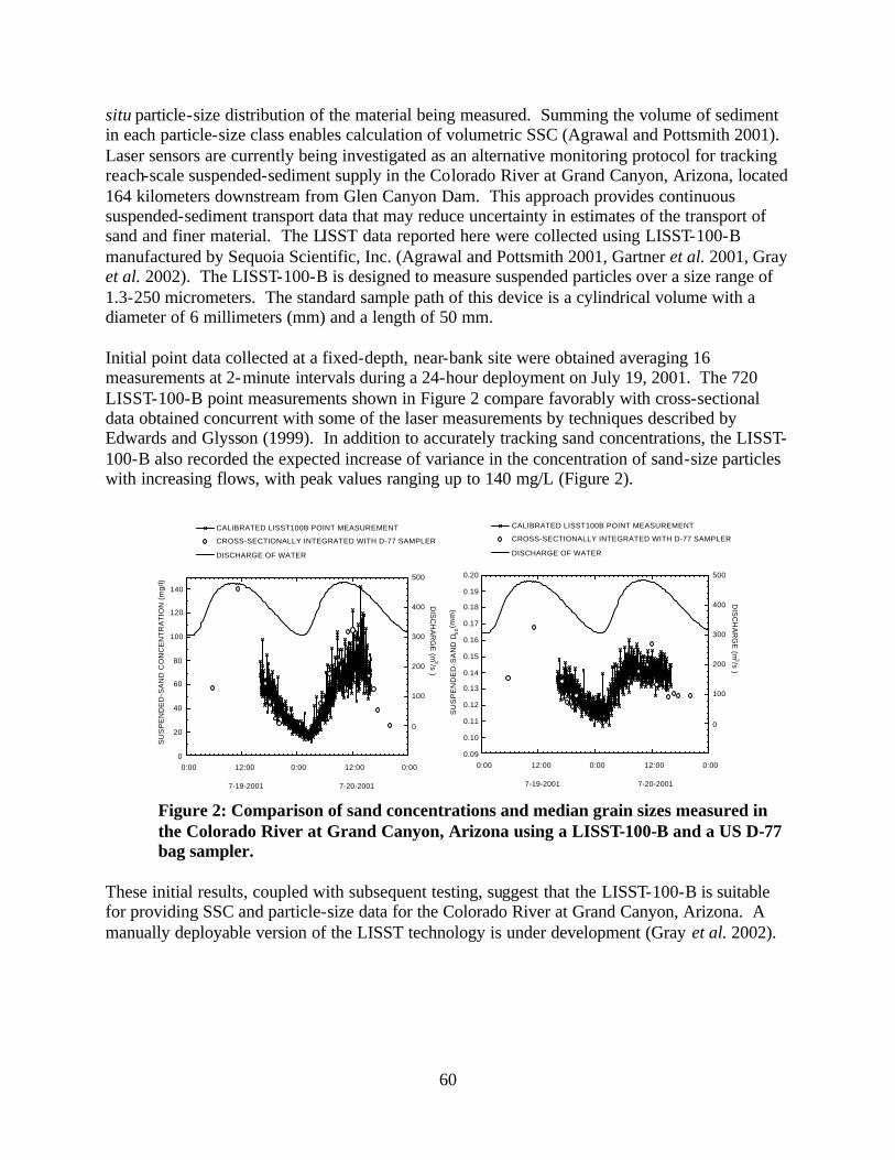
60

situ particle-size distribution of the material being measured. Summing the volume of sediment in each particle-size class enables calculation of volumetric SSC (Agrawal and Pottsmith 2001). Laser sensors are currently being investigated as an alternative monitoring protocol for tracking reach-scale suspended-sediment supply in the Colorado River at Grand Canyon, Arizona, located 164 kilometers downstream from Glen Canyon Dam. This approach provides continuous suspended-sediment transport data that may reduce uncertainty in estimates of the transport of sand and finer material. The LISST data reported here were collected using LISST-100-B manufactured by Sequoia Scientific, Inc. (Agrawal and Pottsmith 2001, Gartner et al. 2001, Gray et al. 2002). The LISST-100-B is designed to measure suspended particles over a size range of 1.3-250 micrometers. The standard sample path of this device is a cylindrical volume with a diameter of 6 millimeters (mm) and a length of 50 mm. Initial point data collected at a fixed-depth, near-bank site were obtained averaging 16 measurements at 2-minute intervals during a 24-hour deployment on July 19, 2001. The 720 LISST-100-B point measurements shown in Figure 2 compare favorably with cross-sectional data obtained concurrent with some of the laser measurements by techniques described by Edwards and Glysson (1999). In addition to accurately tracking sand concentrations, the LISST-100-B also recorded the expected increase of variance in the concentration of sand-size particles with increasing flows, with peak values ranging up to 140 mg/L (Figure 2).

0

20

40

60

80

100

120

140

CALIBRATED LISST100B POINT MEASUREMENT

CROSS-SECTIONALLY INTEGRATED WITH D-77 SAMPLER

DISCHARGE OF WATER

0

100

200

300

400

500

0:00 12:00 0:00 12:00 0:00

SU

SP

EN

DE

D-S

AN

D C

ON

CE

NT

RA

TIO

N (

mg/

l)

DIS

CH

AR

GE

(m3/s

)

7-19-2001 7-20-2001

0.09

0.10

0.11

0.12

0.13

0.14

0.15

0.16

0.17

0.18

0.19

0.20

CALIBRATED LISST100B POINT MEASUREMENT

CROSS-SECTIONALLY INTEGRATED WITH D-77 SAMPLER

DISCHARGE OF WATER

0

100

200

300

400

500

0:00 12:00 0:00 12:00 0:00

SU

SP

EN

DE

D-S

AN

D D

50 (

mm

)

DIS

CH

AR

GE

(m3/s

)

7-19-2001 7-20-2001 Figure 2: Comparison of sand concentrations and median grain sizes measured in the Colorado River at Grand Canyon, Arizona using a LISST-100-B and a US D-77 bag sampler.

These initial results, coupled with subsequent testing, suggest that the LISST-100-B is suitable for providing SSC and particle-size data for the Colorado River at Grand Canyon, Arizona. A manually deployable version of the LISST technology is under development (Gray et al. 2002).

61

Photo-Optic Imaging Data as Laboratory and Stream Suspended-Sediment Surrogates: Photo-optic imaging of fluids was pioneered by the medical industry in the 1980’s for determining red blood cell concentrations. This technology, which is used to delineate, characterize, and enumerate organic particles in blood samples, is being adapted to quantify the concentration and selected size and shape characteristics of suspended sediments in water samples. Research to apply photo-optic imaging for laboratory (Gooding 2001) and field applications is centered at the U.S. Geological Survey’s Cascades Volcano Observatory in Vancouver, Washington (U.S. Geological Survey 2003). Photo-optic imaging has the capability to provide in real time suspended-sediment concentrations, and measurements of the size and shape of individual particles in addition to statistics on size and shape for all particles. Laboratory applications include concentration and size-fraction determinations in addition to shape computations. Potential field applications include automatic point measurements and manual measurements as part of a modified depth-integrating sampler (Edwards and Glysson 1999, Gray et al. 2002). The technology uses lens, fiber-optic cable, a flow-through cell, and a camera with “frame-grabbing” capabilities to obtain a two-dimensional image of suspended solid-phase particles either in a stream or in a re-suspended sample. The physical viewing area of the flow-through cell has a diameter of 10 millimeters (mm) and an internal depth of 4 mm. The lens and flow-through cell were custom built to match the flow-through cell dimensions. Other parts are commercially available. A captured high-quality image is automatically converted to a binary image with distinguished particle boundaries using Matrox Inspector with MIL 7.0 Imaging Library software (Matrox Imaging 2003). This morphologically transformed image usually has fewer details than appear in the original photograph, implying a loss of information. However, the size and shape characteristics in the transformed image remain readily quantifiable. Once an image has been simplified by morphological transformation, quantitative analysis is conducted on the image. Inherent complexities involved with imaging individual sediment particles in a liquid medium impede extraction of usable information from two-dimensional images. However, as illustrated below, hardware enhancements have improved the quality of the image resulting in more reliable automated computer interpretations. An unfiltered lens tends to give unreliable results for transparent particles, but polarizing the light used to illuminate the target area eliminates this problem. By combining two in- line polarized filters from 50° to 70° from cross polarization between the illumination source and target area, all particles, become completely darkened but still maintain the requisite contrast with the background as demonstrated in Figure 3. The presence of turbidity caused by organic and colloidal material also can hinder obtaining a useable image for analysis. Using a near-ultraviolet wavelength of 450 – 500 nanometers to illuminate the target area results in a decrease in reflectance and refraction, as seen when using visible-wavelength spectrum lighting. Images of particles—“blobs”—suspended within turbid water are shown in Figure 4. The water-sediment mixture in this image has a concentration of

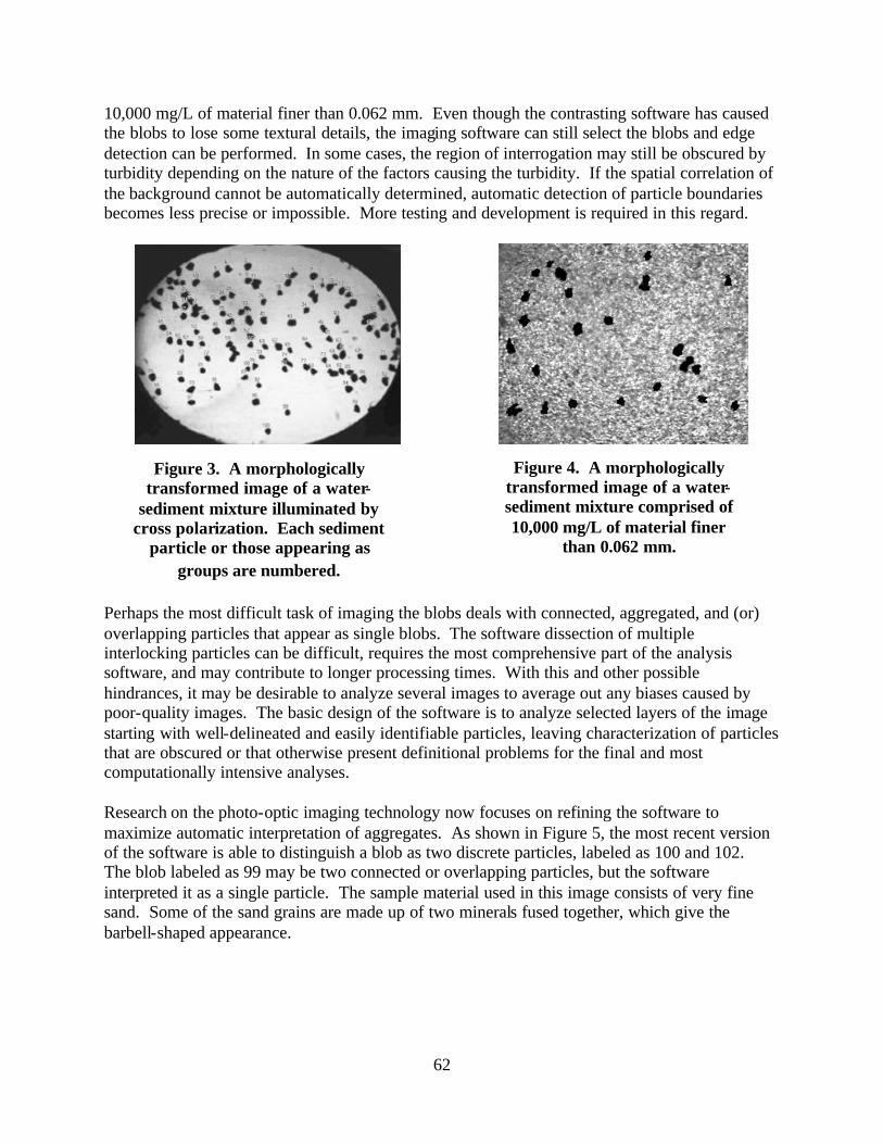
62

10,000 mg/L of material finer than 0.062 mm. Even though the contrasting software has caused the blobs to lose some textural details, the imaging software can still select the blobs and edge detection can be performed. In some cases, the region of interrogation may still be obscured by turbidity depending on the nature of the factors causing the turbidity. If the spatial correlation of the background cannot be automatically determined, automatic detection of particle boundaries becomes less precise or impossible. More testing and development is required in this regard.

Perhaps the most difficult task of imaging the blobs deals with connected, aggregated, and (or) overlapping particles that appear as single blobs. The software dissection of multiple interlocking particles can be difficult, requires the most comprehensive part of the analysis software, and may contribute to longer processing times. With this and other possible hindrances, it may be desirable to analyze several images to average out any biases caused by poor-quality images. The basic design of the software is to analyze selected layers of the image starting with well-delineated and easily identifiable particles, leaving characterization of particles that are obscured or that otherwise present definitional problems for the final and most computationally intensive analyses. Research on the photo-optic imaging technology now focuses on refining the software to maximize automatic interpretation of aggregates. As shown in Figure 5, the most recent version of the software is able to distinguish a blob as two discrete particles, labeled as 100 and 102. The blob labeled as 99 may be two connected or overlapping particles, but the software interpreted it as a single particle. The sample material used in this image consists of very fine sand. Some of the sand grains are made up of two minerals fused together, which give the barbell-shaped appearance.

Figure 4. A morphologically transformed image of a water-sediment mixture comprised of 10,000 mg/L of material finer

than 0.062 mm.

Figure 3. A morphologically transformed image of a water-

sediment mixture illuminated by cross polarization. Each sediment

particle or those appearing as groups are numbered.

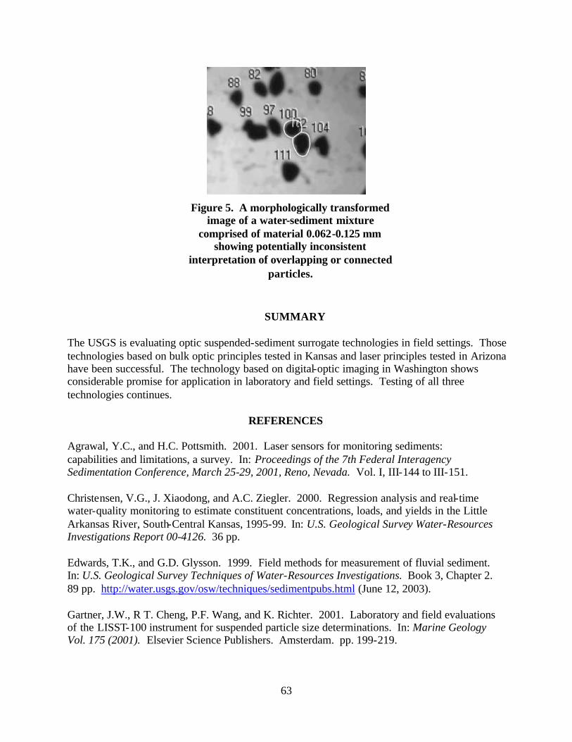
63

SUMMARY

The USGS is evaluating optic suspended-sediment surrogate technologies in field settings. Those technologies based on bulk optic principles tested in Kansas and laser principles tested in Arizona have been successful. The technology based on digital-optic imaging in Washington shows considerable promise for application in laboratory and field settings. Testing of all three technologies continues.

REFERENCES Agrawal, Y.C., and H.C. Pottsmith. 2001. Laser sensors for monitoring sediments: capabilities and limitations, a survey. In: Proceedings of the 7th Federal Interagency Sedimentation Conference, March 25-29, 2001, Reno, Nevada. Vol. I, III-144 to III-151. Christensen, V.G., J. Xiaodong, and A.C. Ziegler. 2000. Regression analysis and real-time water-quality monitoring to estimate constituent concentrations, loads, and yields in the Little Arkansas River, South-Central Kansas, 1995-99. In: U.S. Geological Survey Water-Resources Investigations Report 00-4126. 36 pp. Edwards, T.K., and G.D. Glysson. 1999. Field methods for measurement of fluvial sediment. In: U.S. Geological Survey Techniques of Water-Resources Investigations. Book 3, Chapter 2. 89 pp. http://water.usgs.gov/osw/techniques/sedimentpubs.html (June 12, 2003). Gartner, J.W., R T. Cheng, P.F. Wang, and K. Richter. 2001. Laboratory and field evaluations of the LISST-100 instrument for suspended particle size determinations. In: Marine Geology Vol. 175 (2001). Elsevier Science Publishers. Amsterdam. pp. 199-219.

Figure 5. A morphologically transformed image of a water-sediment mixture

comprised of material 0.062-0.125 mm showing potentially inconsistent

interpretation of overlapping or connected particles.

64

Gooding, D.J. 2001. Photo-optical sedimentation tube. In: Proceedings of the 7th Federal Interagency Sedimentation Conference, March 25-29, 2001, Reno, Nevada. Vol. 1, Poster 29-30. Gray, J.R. 2002. The need for sediment surrogate technologies to monitor fluvial-sediment Transport. In: Proceedings of the Turbidity and Other Sediment Surrogates Workshop, April 30 - May 2, 2002, Silver Legacy Hotel, Reno, Nevada. 4 pp. http://water.usgs.gov/osw/techniques/TSS/listofabstracts.htm (May 20, 2003). Gray, J.R., E. Patiño, P.P. Rasmussen, M.C. Larsen, T.S. Melis, D.J. Topping, M.S. Runner, and C. F. Alamo. 2003. Evaluation of sediment-surrogate technologies for computation of suspended-sediment transport: In: Proceedings of the 1st International Yellow River Forum on River Basin Management, Yellow River Conservancy Commission, Zhengzhou, Henan Province, China. http://water.usgs.gov/osw/techniques/yrcc_surrogates.pdf (May 20, 2003). Gray, J.R, and G.D. Glysson. 2003. Proceedings of the Federal Interagency Sedimentation Workshop on Turbidity and Other Sediment Surrogates, April 30-May 2, 2002, Reno, Nevada. In: U.S. Geological Circular 1250. http://water.usgs.gov/osw/techniques/turbidity.html (June 30, 2003). Gray, J.R., G.D. Glysson, and D.S. Mueller. 2002. Comparability and accuracy of fluvial-sediment data – a view from the U.S. Geological Survey: In: Proceedings of the ASCE Specialty Conference, Hydraulic Measurements & Experimental Methods Conference, Estes Park, Colorado, July 28-August 1, 2002. 6 pp. http://water.usgs.gov/osw/techniques/asce.pdf (May 20, 2003). Gray, J.R. and L.J. Schmidt. 1998. Sediment technology for the 21st century. In: Proceedings of the Federal Interagency Workshop, February 17-19, 1998, St. Petersburg, Fl. http://water.usgs.gov/osw/techniques/sedtech21/index.html (June 25, 2003). Matrox Imaging. 2003. Matrox Inspector Version 4.1. http://www.matrox.com/imaging/products/inspector/home.cfm (June 27, 2003). Schoellhamer, D. H. 2001. Continuous monitoring of suspended sediment in rivers by use of optical sensors. In: Proceedings of the 7th Federal Interagency Sedimentation Conference, March 25-29, 2001, Reno, Nevada. Vol. 1, III-160 to III-167. U.S. Geological Survey. 2003. Cascades Volcano Observatory. http://vulcan.wr.usgs.gov/ (June 24, 2003).

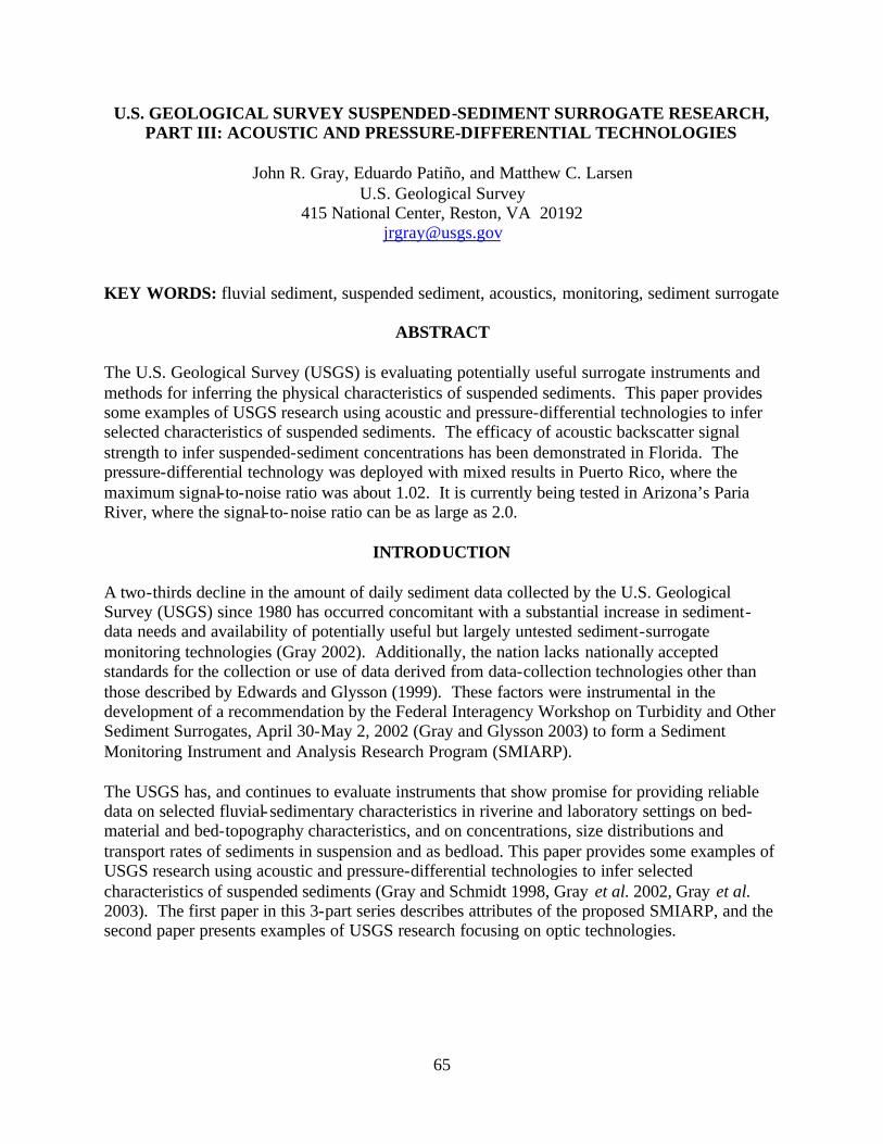
65

U.S. GEOLOGICAL SURVEY SUSPENDED-SEDIMENT SURROGATE RESEARCH, PART III: ACOUSTIC AND PRESSURE-DIFFERENTIAL TECHNOLOGIES

John R. Gray, Eduardo Patiño, and Matthew C. Larsen

U.S. Geological Survey 415 National Center, Reston, VA 20192

jrgray@usgs.gov KEY WORDS: fluvial sediment, suspended sediment, acoustics, monitoring, sediment surrogate

ABSTRACT The U.S. Geological Survey (USGS) is evaluating potentially useful surrogate instruments and methods for inferring the physical characteristics of suspended sediments. This paper provides some examples of USGS research using acoustic and pressure-differential technologies to infer selected characteristics of suspended sediments. The efficacy of acoustic backscatter signal strength to infer suspended-sediment concentrations has been demonstrated in Florida. The pressure-differential technology was deployed with mixed results in Puerto Rico, where the maximum signal-to-noise ratio was about 1.02. It is currently being tested in Arizona’s Paria River, where the signal-to-noise ratio can be as large as 2.0.

INTRODUCTION A two-thirds decline in the amount of daily sediment data collected by the U.S. Geological Survey (USGS) since 1980 has occurred concomitant with a substantial increase in sediment-data needs and availability of potentially useful but largely untested sediment-surrogate monitoring technologies (Gray 2002). Additionally, the nation lacks nationally accepted standards for the collection or use of data derived from data-collection technologies other than those described by Edwards and Glysson (1999). These factors were instrumental in the development of a recommendation by the Federal Interagency Workshop on Turbidity and Other Sediment Surrogates, April 30-May 2, 2002 (Gray and Glysson 2003) to form a Sediment Monitoring Instrument and Analysis Research Program (SMIARP). The USGS has, and continues to evaluate instruments that show promise for providing reliable data on selected fluvial-sedimentary characteristics in riverine and laboratory settings on bed-material and bed-topography characteristics, and on concentrations, size distributions and transport rates of sediments in suspension and as bedload. This paper provides some examples of USGS research using acoustic and pressure-differential technologies to infer selected characteristics of suspended sediments (Gray and Schmidt 1998, Gray et al. 2002, Gray et al. 2003). The first paper in this 3-part series describes attributes of the proposed SMIARP, and the second paper presents examples of USGS research focusing on optic technologies.

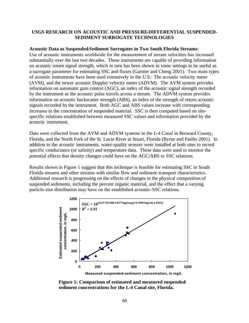
66

USGS RESEARCH ON ACOUSTIC AND PRESSURE-DIFFERENTIAL SUSPENDED-SEDIMENT SURROGATE TECHNOLOGIES

Acoustic Data as Suspended-Sediment Surrogates in Two South Florida Streams: Use of acoustic instruments worldwide for the measurement of stream velocities has increased substantially over the last two decades. These instruments are capable of providing information on acoustic return signal strength, which in turn has been shown in some settings to be useful as a surrogate parameter for estimating SSC and fluxes (Gartner and Cheng 2001). Two main types of acoustic instruments have been used extensively in the U.S.: The acoustic velocity meter (AVM), and the newer acoustic Doppler velocity meter (ADVM). The AVM system provides information on automatic gain control (AGC), an index of the acoustic signal strength recorded by the instrument as the acoustic pulse travels across a stream. The ADVM system provides information on acoustic backscatter strength (ABS), an index of the strength of return acoustic signals recorded by the instrument. Both AGC and ABS values increase with corresponding increases in the concentration of suspended material. SSC is then computed based on site-specific relations established between measured SSC values and information provided by the acoustic instrument. Data were collected from the AVM and ADVM systems in the L-4 Canal in Broward County, Florida, and the North Fork of the St. Lucie River at Stuart, Florida (Byrne and Patiño 2001). In addition to the acoustic instruments, water-quality sensors were installed at both sites to record specific conductance (or salinity) and temperature data. These data were used to monitor the potential effects that density changes could have on the AGC/ABS to SSC relations. Results shown in Figure 1 suggest that this technique is feasible for estimating SSC in South Florida streams and other streams with similar flow and sediment-transport characteristics. Additional research is progressing on the effects of changes in the physical composition of suspended sediments, including the percent organic material, and the effect that a varying particle-size distribution may have on the established acoustic-SSC relations.

0

200

400

600

800

1000

1200

0 200 400 600 800 1000 1200

Measured suspended-sediment concentration, in mg/L

Est

imat

ed s

uspe

nded

-sed

imen

tco

ncen

trat

ion,

in m

g/L

Figure 1: Comparison of estimated and measured suspended-sediment concentrations for the L-4 Canal site, Florida.

SSC = 10{AGC*[0.1968-0.017*log(temp)]+0.7096*log(vel)-4.4561]} R2 = 0.91

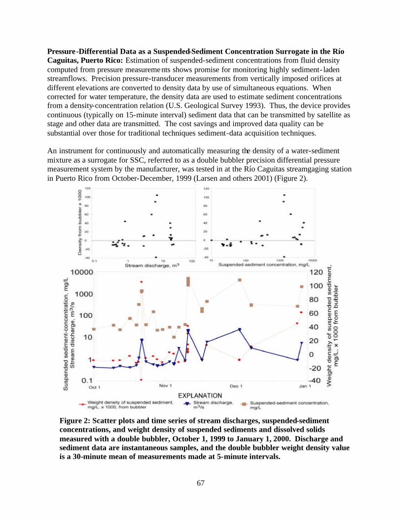
67

Pressure-Differential Data as a Suspended-Sediment Concentration Surrogate in the Río Caguitas, Puerto Rico: Estimation of suspended-sediment concentrations from fluid density computed from pressure measurements shows promise for monitoring highly sediment- laden streamflows. Precision pressure-transducer measurements from vertically imposed orifices at different elevations are converted to density data by use of simultaneous equations. When corrected for water temperature, the density data are used to estimate sediment concentrations from a density-concentration relation (U.S. Geological Survey 1993). Thus, the device provides continuous (typically on 15-minute interval) sediment data that can be transmitted by satellite as stage and other data are transmitted. The cost savings and improved data quality can be substantial over those for traditional techniques sediment-data acquisition techniques. An instrument for continuously and automatically measuring the density of a water-sediment mixture as a surrogate for SSC, referred to as a double bubbler precision differential pressure measurement system by the manufacturer, was tested in at the Río Caguitas streamgaging station in Puerto Rico from October-December, 1999 (Larsen and others 2001) (Figure 2).

Figure 2: Scatter plots and time series of stream discharges, suspended-sediment concentrations, and weight density of suspended sediments and dissolved solids measured with a double bubbler, October 1, 1999 to January 1, 2000. Discharge and sediment data are instantaneous samples, and the double bubbler weight density value is a 30-minute mean of measurements made at 5-minute intervals.

68

The data collected during October-December 1999 at this site showed relatively poor agreement between discharge, SSC, and water density (Figure 2). The 1999 tests indicate that the double bubbler instrument values generally track substantial variations in SSC, but a large amount of signal noise remains. The maximum SSC measured at the site as of 2000 – 17,700 mg/L – corresponds to a signal-to-noise ratio of about 1.02 This test of the double bubbler instrument showed the need for temperature compensation, and possibly the need to deploy the instrument at a site where the signal-to-noise ratio is substantially larger than 1.02 for the bulk of the runoff hydrograph. The double bubbler is being tested in Arizona’s Paria River, where SSC in excess of a 1 x 106 mg/L have been measured, yielding a signal-to-noise ratio of about 2.0. If adequate results can be achieved, increases in data accuracy and substantial reductions in costs of sediment monitoring programs for rivers carrying moderate-to-large SSC can be realized.

SUMMARY The USGS is evaluating acoustic and pressure-differential suspended-sediment surrogate technologies. Acoustic technology tests in Florida have been successful, and USGS acoustics research is expanding to other states. Results of pressure-differential technology tests in Puerto Rico were inconclusive; this technology is now being tested in the Paria River in Arizona.

REFERENCES

Byrne, M.J., and E. Patiño. 2001. Feasibility of using acoustic and optical backscatter instruments for estimating total suspended solids concentrations in estuarine environments. In: Proceedings of the 7th Federal Interagency Sedimentation Conference, March 25-29, Reno, Nevada. Vol. I, III-135 to III-138. Edwards, T.K., and G.D. Glysson. 1999. Field methods for measurement of fluvial sediment. In: U.S. Geological Survey Techniques of Water-Resources Investigations. Book 3, Chapter 2. 89 pp. http://water.usgs.gov/osw/techniques/sedimentpubs.html (June 12, 2003). Gartner, J.W., and R.T. Cheng. 2001. The promises and pitfalls of estimating suspended solids based on backscatter intensity from acoustic Doppler current profiler. In: Proceedings of the 7th Federal Interagency Sedimentation Conference, March 25-29, 2001, Reno, Nevada. Vol. 1, III-119 to III-126. Gray, J.R. 2002. The need for sediment surrogate technologies to monitor fluvial-sediment transport. In: Proceedings of the Turbidity and Other Sediment Surrogates Workshop, April 30 - May 2, 2002, Silver Legacy Hotel, Reno, Nevada. 4 pp. http://water.usgs.gov/osw/techniques/TSS/listofabstracts.htm (May 20, 2003).

69

Gray, J.R., E. Patiño, P.P. Rasmussen, M.C. Larsen, T.S. Melis, D.J. Topping, M.S. Runner, and C.F. Alamo. 2003. Evaluation of sediment-surrogate technologies for computation of suspended-sediment transport. In: Proceedings of the 1st International Yellow River Forum on River Basin Management, Yellow River Conservancy Commission, Zhengzhou, Henan Province, China. http://water.usgs.gov/osw/techniques/yrcc_surrogates.pdf (May 20, 2003). Gray, J.R, and G.D. Glysson. 2003. Proceedings of the Federal Interagency Sedimentation Workshop on Turbidity and Other Sediment Surrogates, April 30-May 2, 2002, Reno, Nevada. In: U.S. Geological Circular 1250. http://water.usgs.gov/osw/techniques/turbidity.html (June 30, 2003). Gray, J.R., Glysson, G.D., and Mueller, D.S. 2002. Comparability and accuracy of fluvial-sediment data—a view from the U.S. Geological Survey. In: Proceedings of the ASCE Specialty Conference, Hydraulic Measurements & Experimental Methods Conference, Estes Park, Colorado, July 28-August 1, 2002. 6 pp. http://water.usgs.gov/osw/techniques/asce.pdf (May 20, 2003). Gray, J.R. and L.J. Schmidt. 1998. Sediment technology for the 21st century. In: Proceedings of the Federal Interagency Workshop, February 17-19, 1998, St. Petersburg, Fl. http://water.usgs.gov/osw/techniques/sedtech21/index.html (June 25, 2003). Larsen, M.C., C.F. Alamo, C., J.R. Gray, and William Fletcher. 2001. Continuous automated sensing of streamflow density as a surrogate for suspended-sediment concentration sampling. In: Proceedings of the 7th Federal Interagency Sedimentation Conference, March 25-29, Reno, Nevada. Vol. I, III-102 to III-109. U.S. Geological Survey. 1993. Policy and technical guidance for conversion of sediment concentration from parts per million (ppm) to milligrams per liter (mg/L). In: U.S. Geological Survey Office of Surface Water Technical Memorandum 93.21. http://water.usgs.gov/admin/memo/SW/sw93.21.html (May 20, 2003).

70

A PRELIMINARY STUDY OF RAINFALL AND AMMONIUM IN THE SHENANDOAH VALLEY

Wayne S. Teel, Derek Dauberman, and Matthew Martin

Department of Integrated Science and Technology, James Madison University Harrisonburg, VA 22807

teelws@jmu.edu

KEY WORDS: ammonium, poultry, precipitation, rainfall

ABSTRACT The Shenandoah Valley of Virginia has many poultry houses thought to be the cause of increased ammonium deposition. This study found that there is a strong seasonal increase in ammonium concentration throughout the valley, and that close proximity to these houses shows even more impact. The study is in its early stages and expects more complete results over the next five years.

INTRODUCTION The Chesapeake Bay Program (CBP) and the Environmental Protection Agency (EPA) are actively seeking ways to reduce nutrient loads in streams of the Chesapeake Bay watershed. Attention has focused on nitrate and phosphate as chief eutrophication agents once waters reach the bay. These are not the soul source of nutrients (Bricker et al. 1999). As everyone who approaches or steps into a poultry house, home to thousands of rapidly growing chickens or turkeys, the strong smell of ammonia and related compounds also play a role. Quantifying that role is one of the goals of the CBP. In the spring of 2002 the Integrated Science and Technology Department at James Madison University (JMU) was awarded a grant from the CBP to establish a site for the National Trends Network (NTN) and the National Atmospheric Deposition Program (NADP). The lead author is Principle Investigator of this project. These sites collect rainfall on a weekly basis, using a very tight protocol and standardized methods (NADP 1999). Conductivity and pH of the rainfall samples are measured in the field, and then sent to the Central Analytical Laboratory at Illinois State University for further analysis. There they again measure conductivity and pH, then test Ca, Mg, K, NH4, NO3, Cl, SO4, and PO4. Site location for the NADP work is strictly regulated. It must be specific distances from major highways and cites, be limited to nearby traffic, and be at least one mile from the nearest poultry operation. In Rockingham County these citing criteria are difficult to meet, but the JMU Farm, about 12 miles southeast of the main campus in Harrisonburg, near the small town of Port Republic, met these standards. Testing for ammonium in the Shenandoah Valley requires additional collection points. Ammonia is both volatile and highly soluble and does not stay in the atmosphere as long as

71

nitrate. Most rather quickly combines with water in the atmosphere making ammonium hydroxide. This further reacts with acids in the atmosphere, both nitric and sulfuric acids are known to be present along with carbonic acid, making the ammonium ions the parameter to quantify. This ion settles as wet deposition in rainfall or dry deposition, coming out of poultry houses in small particulate matter (Bricker et al. 1999). Our study focuses specifically on wet deposition, looking at rainfall at varying distances from active poultry houses. We started in October of 2002, collecting data from three sites in addition to the NADP site at the JMU Farm, and have found significant results.

METHODS A rainfall gauge and wet/dry collection bucket system, supplied by the Chesapeake Bay Program of the EPA and standardized by the NTN and NADP, were set up at the JMU Farm in June of 2002. Weekly measurement of rainfall began July 1, 2002, and the first measurable rain was recorded the week ending July 16, 2002. Collections occur weekly according to protocol. Collected rainfall is taken to the lab; conductivity and pH are measured with NADP approved equipment, and the remaining sample is then sent to the Central Analytical Laboratory of the Illinois State Water Survey for further analysis. After three to four months their results are returned to us for evaluation. If possible we kept a 50 mL sample of this rainfall for analysis in our laboratory at JMU. In addition to the conductivity tests mentioned above, a small sample is run through the Dionex DX-100 Ion Chromatograph (IC) (AS14 4mm(10-32)), to quantify nitrate, phosphate, and sulfate content. Another 25 mL sample is used to test for the ammonium ion, NH4

+, using the Phenate Method (phenolhypochlorite method) as outlined in Standard Methods 19th edition, pages 4-80-81 (Eaton et al. 1995). This is a colorimetric method using NH4Cl standards. We ran samples though the IC and Phenate tests bimonthly, for a total of 4 testing periods, with a total of 25 to 40 samples each period. Prior to testing, samples were kept in a dark refrigerator to avoid algae growth and other complications. In October and November of 2002, three additional rainfall collection sites were added, using a 4-inch (10 cm) diameter All Weather Rain Gauge. These gauges have an interior graduated cylinder marked to measure to the nearest hundredth of an inch. In order to have enough water to do the testing described above a minimum of 0.15 inches of rain must fall. Rainfall events with lower precipitation totals were discarded, and were not included in total rainfall for the ammonium calculations. The three sites chosen have differing relationships with valley poultry farms. The Dove Farm, has two double-decked chicken houses, holding up to 24,000 birds each. They run between 6 and seven batches of chickens through the houses each year. The gauge is 75 feet from the nearest house and is attached to a split rail fence. The Teel Farm site is located 1500 feet north of the Dove Farm. At least three other poultry houses are within one mile of this farm. The final site, at the Tucker house, is in a rural development in Augusta County not far from Churchville. There are no poultry operations within a mile of this site. Rainfall at all of these sites was collected in the morning after the rainfall event and stored in a refrigerator until testing could take place.

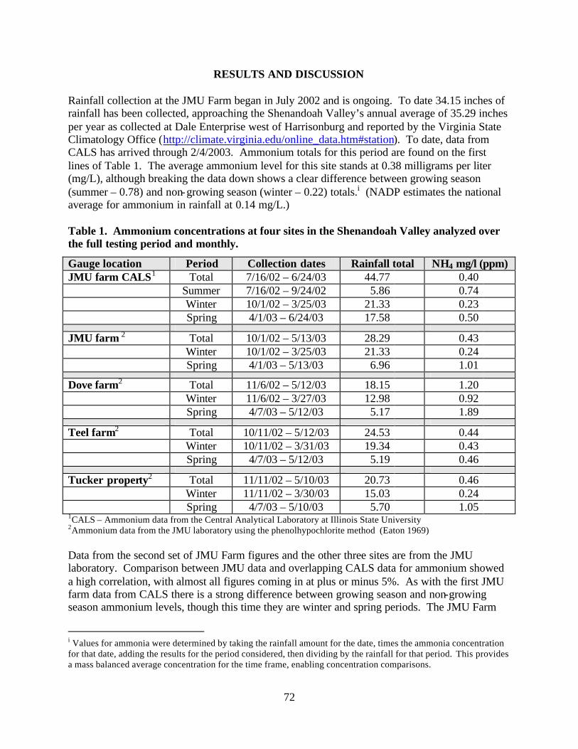
72

RESULTS AND DISCUSSION Rainfall collection at the JMU Farm began in July 2002 and is ongoing. To date 34.15 inches of rainfall has been collected, approaching the Shenandoah Valley’s annual average of 35.29 inches per year as collected at Dale Enterprise west of Harrisonburg and reported by the Virginia State Climatology Office (http://climate.virginia.edu/online_data.htm#station). To date, data from CALS has arrived through 2/4/2003. Ammonium totals for this period are found on the first lines of Table 1. The average ammonium level for this site stands at 0.38 milligrams per liter (mg/L), although breaking the data down shows a clear difference between growing season (summer – 0.78) and non-growing season (winter – 0.22) totals.i (NADP estimates the national average for ammonium in rainfall at 0.14 mg/L.) Table 1. Ammonium concentrations at four sites in the Shenandoah Valley analyzed over the full testing period and monthly.

Gauge location Period Collection dates Rainfall total NH4 mg/l (ppm) JMU farm CALS1 Total 7/16/02 – 6/24/03 44.77 0.40 Summer 7/16/02 – 9/24/02 5.86 0.74 Winter 10/1/02 – 3/25/03 21.33 0.23 Spring 4/1/03 – 6/24/03 17.58 0.50 JMU farm 2 Total 10/1/02 – 5/13/03 28.29 0.43 Winter 10/1/02 – 3/25/03 21.33 0.24 Spring 4/1/03 – 5/13/03 6.96 1.01 Dove farm2 Total 11/6/02 – 5/12/03 18.15 1.20 Winter 11/6/02 – 3/27/03 12.98 0.92 Spring 4/7/03 – 5/12/03 5.17 1.89 Teel farm2 Total 10/11/02 – 5/12/03 24.53 0.44 Winter 10/11/02 – 3/31/03 19.34 0.43 Spring 4/7/03 – 5/12/03 5.19 0.46 Tucker property2 Total 11/11/02 – 5/10/03 20.73 0.46 Winter 11/11/02 – 3/30/03 15.03 0.24 Spring 4/7/03 – 5/10/03 5.70 1.05 1CALS – Ammonium data from the Central Analytical Laboratory at Illinois State University 2Ammonium data from the JMU laboratory using the phenolhypochlorite method (Eaton 1969) Data from the second set of JMU Farm figures and the other three sites are from the JMU laboratory. Comparison between JMU data and overlapping CALS data for ammonium showed a high correlation, with almost all figures coming in at plus or minus 5%. As with the first JMU farm data from CALS there is a strong difference between growing season and non-growing season ammonium levels, though this time they are winter and spring periods. The JMU Farm

i Values for ammonia were determined by taking the rainfall amount for the date, times the ammonia concentration for that date, adding the results for the period considered, then dividing by the rainfall for that period. This provides a mass balanced average concentration for the time frame, enabling concentration comparisons.

73

and the Tucker Property show nearly identical numbers. The strong upswing in ammonium during the spring was surprising not for the amount, but for the similarity. The Teel Farm is more difficult to explain. It shows no significant seasonal variation to date. The Dove Farm, not surprisingly, shows the highest ammonium levels. This too shows strong seasonal variation, though the base level is much higher. Proximity to the houses is the clear cause, and there is strong variation in concentration thought to be due to the presence and age of the birds in the poultry house. According to the Natural Resources Conservation Service (NRCS), the main season for spreading poultry liter in Rockingham and Augusta Counties begins in mid-March and runs through mid-May (Bill Patterson, personal communication). Spreading poultry liter does not necessarily occur on land within site of the poultry house. In many cases poultry farmers produce more litter than their land can handle, so they are required by the NRCS and the state Department of Agriculture to include other land for spreading in their nutrient management plan. For example, the Teel Farm spreads poultry litter on its pastureland as part of the Dove Farm’s nutrient management plan for the two houses. This litter was spread in late March and early April, and rainfall during this time contained the highest ammonium levels of the spring (1.89 mg/L on April 4, 2003). Litter distribution is likely the cause for the high spring ammonia levels, though it does not explain the summer levels. By comparison, the national average for ammonium concentrations at NADP sites varies between less than 0.15 ppm in the Pacific Northwest and Florida, and greater than 0.55 ppm in the upper Midwest centered around the Missouri River Valley from Iowa and Nebraska to North Dakota (NADP 2003). Northern Virginia and the Shenandoah Valley show a consistent annual average ammonium concentration of between 0.20 and 0.25 ppm. This is based on data from their site at Big Meadows along Skyline Drive in Shenandoah National Park. Data from the JMU Farm is not yet included in their web accessible database. Our data shows a near doubling of this total ammonium to 0.40 based on available data. To date we have not completed a full year cycle at any of the sites, nor has an examination started on other possible sources of ammonium, such as anhydrous ammonia fertilization, other ammonia based fertilizers, or dairy and cattle operations. Over the coming months more rainfall collection sites will be added to the ones now in place. These will increase our geographic and farm diversity, providing a better picture of wet deposition. In addition we hope to begin some dry deposition work, also funded through the CBP. The goal is to provide a better picture of ammonium deposition as a source of nutrient in the Chesapeake Bay and to then devise ways to reduce that nutrient load.

74

ACKNOWLEDGMENTS We would like to thank Margaret Kerchner of the Chesapeake Bay Program for her advice and assistance on this project. Thanks also go to the Dove Farm for permission to set up a rain gauge near their poultry houses, and to Gene Tucker for the same near his home – and collecting the rainfall data. Final thanks go to Fred Copithorn, manager of the environmental lab in the Integrated Science and Technology Program at JMU for his assistance with the ammonium wet lab.

REFERENCES Bricker, S.B., C.G. Clement, D.E. Pirhalla, S.P. Orlando, and D.R.G. Farrow. 1999. National Estuarine Eutrophication Assessment: Effects of Nutrient Emissions in the Nation’s Estuaries. http://spo.nos.noaa.gov/projects/cads/nees/Eutro_Report.pdf (January 15, 2004) Eaton, A.D., L.S. Clesceri, and A.E. Greenberg. 1995. Standard Methods for the Examination of Water and Wastewater. American Public Health Association, American Water Works Association, Water Environment Federation. Washington, D.C. National Atmospheric Deposition Program (NADP). 1999. National Trends Network Site Operation Manual. http://nadp.sws.uiuc.edu/lib/manuals/opman.pdf (January 15, 2004). National Atmospheric Deposition Program (NADP). 2003. National Trends Network. http://nadp.sws.uiuc.edu/amaps/nh4/nh4.ppt. (January 15, 2004).

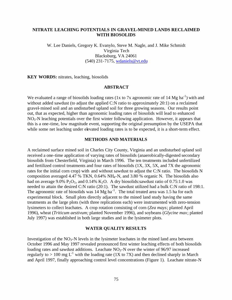
75

NITRATE LEACHING POTENTIALS IN GRAVEL-MINED LANDS RECLAIMED WITH BIOSOLIDS

W. Lee Daniels, Gregory K. Evanylo, Steve M. Nagle, and J. Mike Schmidt

Virginia Tech Blacksburg, VA 24061

(540) 231-7175, wdaniels@vt.edu

KEY WORDS: nitrates, leaching, biosolids

ABSTRACT We evaluated a range of biosolids loading rates (1x to 7x agronomic rate of 14 Mg ha-1) with and without added sawdust (to adjust the applied C:N ratio to approximately 20:1) on a reclaimed gravel-mined soil and an undisturbed upland soil for three growing seasons. Our results point out, that as expected, higher than agronomic loading rates of biosolids will lead to enhanced NO3-N leaching potentials over the first winter following application. However, it appears that this is a one-time, low magnitude event, supporting the original presumption by the USEPA that while some net leaching under elevated loading rates is to be expected, it is a short-term effect.

METHODS AND MATERIALS A reclaimed surface mined soil in Charles City County, Virginia and an undisturbed upland soil received a one-time application of varying rates of biosolids (anaerobically-digested secondary biosolids from Chesterfield, Virginia) in March 1996. The ten treatments included unfertilized and fertilized control treatments and four rates of biosolids (1X, 3X, 5X, and 7X the agronomic rates for the initial corn crop) with and without sawdust to adjust the C:N ratio. The biosolids N composition averaged 4.47 % TKN, 0.64% NH4-N, and 3.80 % organic N. The biosolids also had on average 9.0% P2O5, and 0.14% K2O. A dry biosolids:sawdust ratio of 0.75:1.0 was needed to attain the desired C:N ratio (20:1). The sawdust utilized had a bulk C:N ratio of 198:1. The agronomic rate of biosolids was 14 Mg ha-1. The total treated area was 1.5 ha for each experimental block. Small plots directly adjacent to the mined land study having the same treatments as the large plots (with three replications each) were instrumented with zero-tension lysimeters to collect leachates. A crop rotation consisting of corn (Zea mays; planted April 1996), wheat (Triticum aestivum; planted November 1996), and soybeans (Glycine max; planted July 1997) was established in both large studies and in the lysimeter plots.

WATER QUALITY RESULTS

Investigation of the NO3-N levels in the lysimeter leachates in the mined land area between October 1996 and May 1997 revealed pronounced first winter leaching effects of both biosolids loading rates and sawdust additions. Leachate NO3-N over the winter of 96/97 increased regularly to > 100 mg L-1 with the loading rate (1X to 7X) and then declined sharply in March and April 1997, finally approaching control level concentrations (Figure 1). Leachate nitrate-N

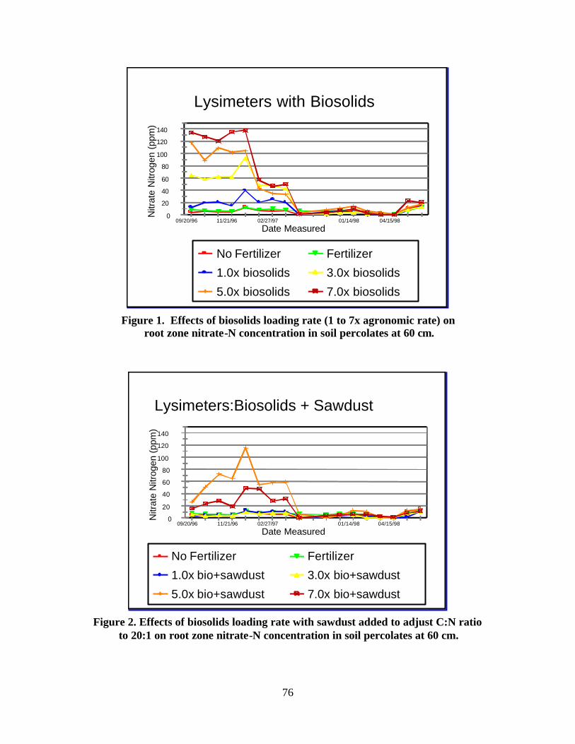
76

0

20

40

60

80

100

120

140

Nitr

ate

Nitr

ogen

(pp

m)

09/20/96 11/21/96 02/27/97 01/14/98 04/15/98

Date Measured

No Fertilizer Fertilizer

1.0x biosolids 3.0x biosolids

5.0x biosolids 7.0x biosolids

Lysimeters with Biosolids

Figure 1. Effects of biosolids loading rate (1 to 7x agronomic rate) on

root zone nitrate-N concentration in soil percolates at 60 cm.

0

20

40

60

80

100

120

140

Nitr

ate

Nitr

ogen

(ppm

)

09/20/96 11/21/96 02/27/97 01/14/98 04/15/98

Date Measured

No Fertilizer Fertilizer

1.0x bio+sawdust 3.0x bio+sawdust

5.0x bio+sawdust 7.0x bio+sawdust

Lysimeters:Biosolids + Sawdust

Figure 2. Effects of biosolids loading rate with sawdust added to adjust C:N ratio

to 20:1 on root zone nitrate-N concentration in soil percolates at 60 cm.

77

levels remained below 10 mg L-1 in November and December 1997. The addition of sawdust to the applied biosolids significantly decreased NO3-N leachate levels (Fig. 2) at all biosolids loading rates except the 5X + sawdust treatment, which exhibited a mid-winter spike in excess of 100 mg L-1. Shallow (< 2 m) groundwater immediately down gradient from the 1.5 ha plots was also monitored monthly, and was unaffected by the treatments. Based on these results, we believe that a loading maximum of 5X the agronomic rate for cake and 7X for C:N ratio adjusted materials would be appropriate for further full-scale biosolids application programs on sand and gravel mined lands in the mid-Atlantic region. The effects of biosolids and sawdust additions on the total mass of NO3-N leached over the course of the two-year monitoring period are given in Table 1. Total leaching losses ranged from 4.9 to 59.8 kg/ha, with the vast majority moving the first winter as discussed above. Total leaching losses generally increased with the biosolids loading rate, but not consistently. The addition of sawdust to increase the C:N ratio effectively lowered NO3-N losses in the 1x and 3x rates to levels similar to the unfertilized control, but appeared to have no effect on suppressing mass losses at the 5x and 7x (plus sawdust) loading rates. Thus, the overall interpretation of treatment effects in this experiment varies somewhat when we use mass loss data versus concentration data as discussed above. As a percent of total-N applied in fertilizer or biosolids, the mass losses were lower than expected, ranging only from 0.7 to a maximum of 3.1% of applied N. We suspect that this relatively low and consistent level of percent leaching loss is related to denitrification losses at the higher loading rates.

Table 1. Total N land-applied and subsequently leached as NO3-N over two years.

Treatment Total-N applied in Biosolids

(kg/ha)

Mass NO3–N leached (kg/ha)

Total-N leached

(%) Control 0 5.9 c1 N.A. Fertilized 269 7.6 c 2.8 1X Biosolids 626 19.2 bc 3.1 3X Biosolids 1252 37.4 abc 3.0 5X Biosolids 3130 28.2 abc 0.9 7X Biosolids 4382 59.8 a 1.4 1X + Sawdust 626 4.9 c 0.8 3X + Sawdust 1252 7.6 c 0.6 5X + Sawdust 3130 58.4 ab 1.9 7X + Sawdust 4382 31.9 abc 0.7

1 Mean mass NO3-N levels followed by the same letter are not significantly different (p=0.05).

DISCUSSION AND CONCLUSIONS This overall experiment was designed to test if (1) the optimal biosolids loading rates for one-time application to mined lands would range from approximately 3x to 7x of the standard agronomic rate; (2) if the NO3-N levels in the winter leaching cycle could be reliably related to the loading rate; and (3) whether leachate levels would be controlled by a combination of loading rate and C:N ratio adjustment via sawdust additions.

78

Based on these results, we believe that a loading maximum of 5x the agronomic rate for cake and 7x for C:N ratio adjusted materials would be appropriate for further full-scale biosolids application programs on reclaimed sand and gravel mined lands in the mid-Atlantic region. This conclusion is based on data from this experiment, and upon similar conclusions reached in biosolids loading rate studies in a wide variety of other locations. Obviously, the addition of biosolids at these rates will lead to one-time (first winter) leaching potentials for NO3-N, but their long-term effects on groundwater concentrations in most situations will be minimal. In contrast, the long term beneficial effects of biosolids applications at elevated rates to mined lands are well-documented and will likely persist for multiple growing seasons. Finally, it is important to point out the mass loss of N from these treatments was generally low, and typically represented < 2.0 % of the total-N applied. It should also be pointed out that the particular mine soil landscape utilized here was much higher in productivity potential than the “typical” post-reclamation mined lands of this type, and very few of these sand and gravel mined areas are returned to row crop production. Appropriate biosolids applications would probably elicit much stronger vegetation responses on more typical gravel mine soils in this region than were observed in this study with row crops. The mine soil studied here was finer textured than would be expected on the majority of reclaimed sand and gravel mines in the region. Therefore, we would expect winter leachates to move more rapidly through the subsoils at coarser textured sites, but the overall treatment effect differentials would be similar. Any intensive research effort such as this one answers certain questions while generating new ones. In particular, there is a continued need for further research into the concept of C:N ratio adjustment. Additional knowledge on the effects of differing C:N ratios and C substrates (leaves, sawdust, woodchips, newspapers, etc.) over a wide range of loading values and site conditions would be very beneficial to the development of more effective biosolids management and mined land reclamation strategies. Also, follow-up studies to directly determine the actual magnitude of first winter NO3-N leaching on local groundwater quality should be conducted and specifically compared to NO3-N leaching under conventional fertilizer based revegetation strategies on the same sites.

ACKNOWLEDGMENTS This study was supported by Synagro, and we appreciate the help of Steve McMahon, Sharon Hogan, Jeff Faust, and Bob Peer in our efforts over time. The project site is on the grounds of Shirley Plantation, and we are thankful for the assistance and daily coordina tion of Charles Carter. Field assistance by Robert Hodges, Pam Thomas, Ron Alls, and Mike Genthner is gratefully acknowledged.

79

NITROGEN FORMS IN VIRGINIA SURFACE WATERS: TEMPORAL AND SPATIAL PATTERNS

C.E. Zipper

Department of Crop and Soil Environmental Sciences, Virginia Tech Blacksburg, VA 24061

czip@vt.edu

G.I. Holtzman Department of Statistics, Virginia Tech

Blacksburg, VA 24061 KEY WORDS: surface water quality, nitrate, total Kjeldahl nitrogen, total nitrogen, seasonal Kendall analysis, water-quality trends

ABSTRACT Water monitoring data collected from 157 Virginia water monitoring locations over the 1978 – 1995 period were analyzed. Variables of interest were nitrate-nitrite N (NN); total Kjeldahl N (TKN); and total N (TN) concentrations, as calculated by the sum of NN and TKN forms. Seasonal and overall TN medians were calculated and allocated among NN and TKN components. NN, TKN, and TN trends were analyzed for each location using seasonal Kendall analysis, by ecoregion, and for the state as a whole. The distribution of N among NN and TKN forms varies both seasonally and regionally. TN concentrations were found to be increasing at monitored locations in 5 of the state’s 7 ecoregions over the study period, with the strongest increases occurring as TKN and in the state’s eastern portions.

INTRODUCTION In-stream nitrogen challenges water-quality monitoring and interpretation because waterborne N occurs in several chemical forms. In-stream nitrogen concentrations are commonly measured and reported as nitrate, nitrite, nitrate plus nitrite, ammonium, organic, total Kjeldahl, and total nitrogen forms. In this presentation, we report on an investigation of the relationship among nitrogen forms in Virginia waterways over the 1978 – 1995 period, using water-quality data collected by Virginia Department of Environmental Quality.

METHODS Water monitoring data from 180 Virginia water monitoring locations over the 1978 – 1995 period were analyzed (Zipper et al. 2002). Only observations containing sufficient data to determine total nitrogen (TN) as the sum of nitrate N, nitrite N (whether measured separately or as a combined measure of nitrate-nitrite N, or NN), and total Kjeldahl N (TKN) were used. A preliminary analysis was conducted to identify monitoring locations with limited representation of the study period and/or where point-source effluent was the dominant component of

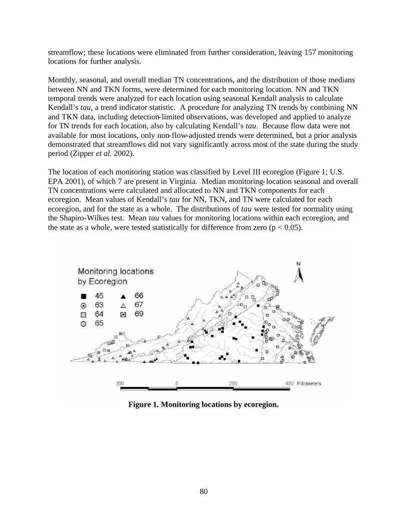
80

streamflow; these locations were eliminated from further consideration, leaving 157 monitoring locations for further analysis. Monthly, seasonal, and overall median TN concentrations, and the distribution of those medians between NN and TKN forms, were determined for each monitoring location. NN and TKN temporal trends were analyzed fo r each location using seasonal Kendall analysis to calculate Kendall’s tau, a trend indicator statistic. A procedure for analyzing TN trends by combining NN and TKN data, including detection- limited observations, was developed and applied to analyze for TN trends for each location, also by calculating Kendall’s tau. Because flow data were not available for most locations, only non-flow-adjusted trends were determined, but a prior analysis demonstrated that streamflows did not vary significantly across most of the state during the study period (Zipper et al. 2002).

The location of each monitoring station was classified by Level III ecoregion (Figure 1; U.S. EPA 2001), of which 7 are present in Virginia. Median monitoring- location seasonal and overall TN concentrations were calculated and allocated to NN and TKN components for each ecoregion. Mean values of Kendall’s tau for NN, TKN, and TN were calculated for each ecoregion, and for the state as a whole. The distributions of tau were tested for normality using the Shapiro-Wilkes test. Mean tau values for monitoring locations within each ecoregion, and the state as a whole, were tested statistically for difference from zero (p < 0.05).

Figure 1. Monitoring locations by ecoregion.

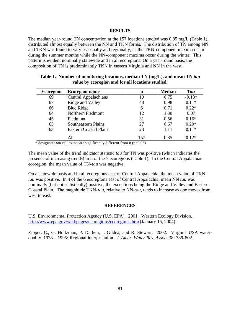
81

RESULTS

The median year-round TN concentration at the 157 locations studied was 0.85 mg/L (Table 1), distributed almost equally between the NN and TKN forms. The distribution of TN among NN and TKN was found to vary seasonally and regionally, as the TKN-component maxima occur during the summer months while the NN-component maxima occur during the winter. This pattern is evident nominally statewide and in all ecoregions. On a year-round basis, the composition of TN is predominantly TKN in eastern Virginia and NN in the west.

Table 1. Number of monitoring locations, median TN (mg/L), and mean TN tau

value by ecoregion and for all locations studied.

Ecoregion Ecoregion name n Median Tau 69 Central Appalachians 10 0.75 -0.13* 67 Ridge and Valley 48 0.98 0.11* 66 Blue Ridge 6 0.71 0.22* 64 Northern Piedmont 12 1.30 0.07 45 Piedmont 31 0.56 0.16* 65 Southeastern Plains 27 0.67 0.20* 63 Eastern Coastal Plain 23 1.11 0.11*

All 157 0.85 0.12* * designates tau values that are significantly different from 0 (p<0.05)

The mean value of the trend indicator statistic tau for TN was positive (which indicates the presence of increasing trends) in 5 of the 7 ecoregions (Table 1). In the Central Appalachian ecoregion, the mean value of TN-tau was negative.

On a statewide basis and in all ecoregions east of Central Appalachia, the mean value of TKN-tau was positive. In 4 of the 6 ecoregions east of Central Appalachia, mean NN tau was nominally (but not statistically) positive, the exceptions being the Ridge and Valley and Eastern Coastal Plain. The magnitude TKN-tau, relative to NN-tau, tends to increase as one moves from west to east.

REFERENCES U.S. Environmental Protection Agency (U.S. EPA). 2001. Western Ecology Division. http://www.epa.gov/wed/pages/ecoregions/ecoregions.htm (January 15, 2004). Zipper, C., G. Holtzman, P. Darken, J. Gildea, and R. Stewart. 2002. Virginia USA water-quality, 1978 – 1995: Regional interpretation. J. Amer. Water Res. Assoc. 38: 789-802.

82

MEASURING WATER VELOCITY PROFILES WITH ACOUSTIC DOPPLER TECHNOLOGY IN A VIRGINIA TAILWATER

Colin Krause

Department of Fisheries and Wildlife Sciences, Virginia Tech 125 Cheatham Hall (0321), Blacksburg, VA 24061

cokrause@vt.edu

Yi Shen Department of Civil and Environmental Engineering, Virginia Tech

Patton Hall, Blacksburg, VA 24061 yishen@vt.edu

KEY WORDS: acoustic Doppler profiler, RiverCat, water velocity, discharge, hydropeaking

ABSTRACT

The two-dimensional flow model RMA-2V was developed for two sections of a hydropeaking tailwater in Virginia as part of a Brown trout fisheries research study. We required known water velocity data at multiple flows to calibrate and validate the model. To measure these velocities at flows too high and swift to wade with a flow meter, we utilized a wireless acoustic Doppler profiler. The floating profiler towed across the channel with a cableway system allowed peak flow water velocities to be safely measured by operators on shore.

INTRODUCTION The trout fishery in the Smith River tailwater below Philpott Dam in southwestern Virginia supports a naturally reproducing brown trout population, as well as stocked rainbow trout. Despite rapidly varying flows (1 to 40 cms in 15 minutes) from the Philpott Dam hydropeaking electric facility, the tailwater supports trout due to a hypolimnetic release (i.e., cold-water). In the 1970s brown trout in the Smith River reached trophy sizes up to 8.2 kg with fish of 4.5 kg not being uncommon (Mohn 2001). However, over the last twenty years, the fishery has rarely produced >4.5 kg trout, and in the last ten years, there are very few catches of trophy size trout (635 mm, 2.3 kg) (Anderson et al. 2003). This is of concern to the Virginia Department of Game and Inland Fisheries (VDGIF) who manage the river from 5.3 to 10 river kilometers (rkm) below the dam for trophy brown trout. Therefore, VDGIF and the Virginia Tech Department of Fisheries and Wildlife Sciences began a 5-year study in 1999 to develop a scientific foundation for supporting alternative flow scenarios that could improve the fishery (Orth et al. 2002). A component of this study developed a two-dimensional hydraulic model to measure the effects of varying flow on shear stress, mobilization of streambed gravels, and the discharge relationship to the amount of spawning-nest scouring or brown trout fry displacement. This information The use of firm or trade names does not constitute a recommendation or endorsement by the Virginia Water Resources Research Center.

83

coupled with flow records can predict catastrophic year-class failures and flow ranges that provide acceptable reproduction. The 2-D hydraulic model (RMA-2V) developed for sections of the Smith River required water velocity data at multiple discharges for calibration and validation purposes. Water velocity is typically measured with flow meters (e.g., models such as Marsh McBirny and Price AA) when flows are shallow (<1m) and slow (<1 m/s) enough for the operator to wade in the river. However, in cases such as the Smith River during peak flow, the river is too deep and swift. The SonTek® RiverCat®, a wireless Acoustic Doppler Profiler (ADP®) with integrated Global Positioning System (GPS) mounted on floating pontoons, enables data collection in unwadeable situations when towed across the river on a portable cableway. Additionally, the RiverCat enables discharge and velocity data collection where there is no bridge or when the river is too small and shallow for a motorized boat. The ADP measures water velocity based on a physical principle called the Doppler effect. When a source of sound is moving relative to the receiver, the frequency of the sound at the receiver is shifted from the transmit frequency: This is the Doppler effect. The ADP emits sound waves and tracks the reflection of the sound waves off particles in the water. The change in frequency of the reflected sound is proportional to the velocity of the water. This technology enables water velocity measurement at multiple profiles across the river channel and at multiple cells from near the water surface to the channel bottom.

METHOD The RMA-2V hydraulic model was developed for a 165 m section at 4.2 rkm and a 200 m section at 12.6 rkm below Philpott Dam that corresponded with trout spawning areas. Water velocity data for model calibration and validation was measured at baseflow (~1.8 cms), moderate flow (~19 cms), and peak flow (~40 cms). Mean column depth velocity at baseflow was measured while wading in the river with a Marsh McBirny® 2000 model flow meter. With the flow meter we measured velocity at 186 locations over 9 transects at the 4.2 rkm site and 194 locations over 10 transects at the 12.6 rkm site. During moderate and peak flows, velocity was measured with the RiverCat. At the 4.2 rkm and 12.6 rkm site, 7 transects (3 at moderate and 4 at peak flow) and 11 transects (7 at moderate and 4 at peak flow) were measured, respectively. At each transect location, the RiverCat was pulled back and forth across the channel multiple times to provide between 2 to 10 replicates for averaging. The RiverCat was set to record velocity in 15 cm cells every 10 seconds. The RiverCat (powered by 16 C-cell batteries) communicates wirelessly with a laptop computer, and we used a Honda® EX350 generator to power the laptop and wireless transceiver. To deploy the RiverCat across the river channel along transects perpendicular to the flow, a portable cableway was built. The cableway consisted of anchoring a CMI® micro pulley on each bank at least 1.5 m above the high-water level to either a tree or tripod. Pulleys were connected with a carabiner to a NRS® tie-down strap looped around either a tree or a Topcon® aluminum tripod secured to the ground with two tie-down straps using screw-type earth anchors. A perlon rope (7 mm diameter) was strung through both pulleys forming a circular loop over the river. The two ends of the rope were connected with a Petzl® basic ascender which allowed the rope to be pulled taught. Different lengths of tie-down straps were used to connect the RiverCat to the rope to facilitate measuring multiple transects from one cableway location. The RiverCat could

84

then be moved back and forth across the channel by pulling the rope through the pulleys. Ideally we set the cableway shortly before the peak flow arrived and water level rose. However, we encountered periods of 24-hr continuous peak flow release which required us to paddle across the river using a Hobie® Float Cat boat to set the cableway.

RESULTS AND DISCUSSION The RiverCat and cableway system enabled us to measure water velocities at high flows when wading with a flow meter is not possible. At baseflow, we used a flow meter because the river depths were less than the 0.55 to 6 m range that the 3.0 MHz frequency ADP requires to function. Other SonTek ADP’s operate at different frequencies and thus can measure different depth ranges (5.0 MHz for 0.3-2.5 m and 1.5 MHz for 0.8-25 m). Faster water velocity occurred at higher flows and in the middle of the channel where depth was greatest (Figure 1). Friction caused by the channel bottom in shallow water near the banks lessened the velocity such that moderate and peak flow velocities were similar. Based on depth measurements averaged across the channel, the water surface elevation increased 1.2 and 1.0 m between base and peak flow at sites 4.2 rkm and 12.6 rkm, respectively. Thus there is a large fluctuation in water level as well as water velocity on a daily basis because of the hydropeaking operation. Measuring each transect multiple times and then plotting a polynomial regression through the data provides a more complete and accurate velocity profile across the channel (Figure 1). The velocity of the RiverCat as it travels across the channel is determined by either the integrated differential global positioning system (GPS) with <1 m error or by bottom tracking. The smaller the width of the river, the greater the relative error of the GPS position becomes. Therefore, we found bottom tracking more accurate than GPS. The GPS locations also allow the overlay of velocity data on the modeled sites in a geographic information system (GIS). Bottom tracking is only accurate when the channel bottom is stationary, thus GPS can be more accurate in cases where the high velocities cause bedload movement. Data comparison between GPS versus bottom tracking revealed bed movement occurred at the 12.6 rkm site during peak flow along some transects. The concept that bedload movement can be observed with an ADP has lead to other uses for this technology such as the measurement of bed load velocity (Rennie et al. 2002). Additionally, suspended sediment concentrations can be measured with an ADP because there is a relationship between ADP signal strength and sediment size, type, and concentration (Sontek 2003).

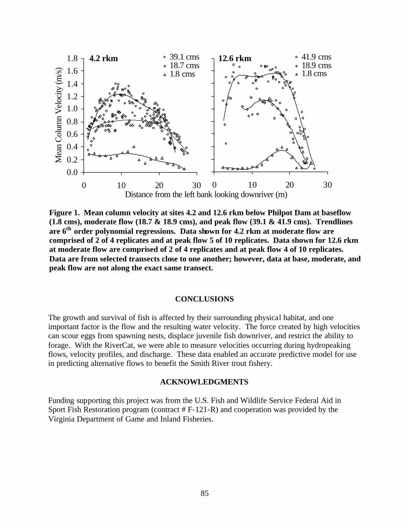
85

Figure 1. Mean column velocity at sites 4.2 and 12.6 rkm below Philpot Dam at baseflow (1.8 cms), moderate flow (18.7 & 18.9 cms), and peak flow (39.1 & 41.9 cms). Trendlines are 6th order polynomial regressions. Data shown for 4.2 rkm at moderate flow are comprised of 2 of 4 replicates and at peak flow 5 of 10 replicates. Data shown for 12.6 rkm at moderate flow are comprised of 2 of 4 replicates and at peak flow 4 of 10 replicates. Data are from selected transects close to one another; however, data at base, moderate, and peak flow are not along the exact same transect.

4.2 rkm

0.00.20.40.60.81.01.21.41.61.8

0 10 20 30

Mea

n C

olum

n V

eloc

ity (m

/s)39.1 cms18.7 cms1.8 cms

12.6 rkm

0 10 20 30

41.9 cms18.9 cms1.8 cms

Distance from the left bank looking downriver (m)

CONCLUSIONS

The growth and survival of fish is affected by their surrounding physical habitat, and one important factor is the flow and the resulting water velocity. The force created by high velocities can scour eggs from spawning nests, displace juvenile fish downriver, and restrict the ability to forage. With the RiverCat, we were able to measure velocities occurring during hydropeaking flows, velocity profiles, and discharge. These data enabled an accurate predictive model for use in predicting alternative flows to benefit the Smith River trout fishery.

ACKNOWLEDGMENTS

Funding supporting this project was from the U.S. Fish and Wildlife Service Federal Aid in Sport Fish Restoration program (contract # F-121-R) and cooperation was provided by the Virginia Department of Game and Inland Fisheries.

86

REFERENCES Anderson, M.R., D.J. Orth, and S.M. Smith. 2003. Historical changes in the Brown trout fishery in the Smith River tailwater, Virginia. Proceedings of the Annual Conference of the Southeastern Association of Fish and Wildlife Agencies. In Review. Mohn, L. 2001. 2001 Trout guide. Virginia Wildlife 62: 6-28. Orth, D.J., T.J. Newcomb, P. Diplas, and A.C. Dolloff. 2002. Influences of Fluctuating Releases on Stream Habitats for Brown Trout in the Smith River Below Philpott Dam. Annual report, Federal Aid for Sport Fish Restoration. Contract No. 08220203. Virginia Department of Game and Inland Fisheries. Richmond, Va. Rennie, C.D., R.G. Millar, and M.A. Church. 2002. Measurement of bed load velocity using an acoustic Doppler current profiler. Journal of Hydraulic Engineering 128(5): 473-483. SonTek. 2003. ADP versatility in San Felipe, Mexico deployment. http://www.sontek.com/apps/profiler/adp-sf/adp-sf.htm (May 27, 2003).

87

FISH HABITAT ASSESSMENT WITH ONE- AND TWO-DIMENSIONAL ECOHYDRAULIC MODELS

Yi Shen and Panayiotis Diplas

Department of Civil Engineering, Virginia Tech Blacksburg, VA, 24061

yishen@vt.edu, pdiplas@vt.edu

KEYWORDS: fish habitat, PHABSIM, RMA2, ecohydraulic model

INTRODUCTION Fishery biologists have expressed interest in the feasibility of enhancing brown trout spawning habitat (i.e., redds) in the Smith River below Philpott Dam in Virginia, which is considered as one of the best brown trout streams in this country (Cochran 1975). Since the Philpott Dam releases daily short-term high flows to the Smith River, it is desirable to explore the role of the altered flow regimes on the stream habitat. Varieties of methods, including one-dimensional (1-D) and two-dimensional (2-D) approaches, have been employed to investigate the instream flow requirements since the late 1970s (e.g., Crowder and Diplas 2000). Up to now, the most widely used numerical program, PHABSIM (Physical HABitat SIMulation) (Bovee 1982), is a 1-D ecohydraulic model. However, the 1-D method cannot account for irregular channel bed topography. To partially remedy this shortcoming, 2-D models have been used increasingly for habitat assessment. A major advantage of the 2-D models is that they can quantify more accurately the highly complex spatial flow patterns, such as eddies and transverse flows (Crowder and Diplas 2000). This paper presents results of a study that examined the predictions of brown trout spawning habitat using 1-D (PHABSIM) and 2-D (RMA2; King 1999) models at a selected site in the Smith River. The performance of the two models was evaluated by a regression analysis, and the differences between the two models are briefly discussed.

METHODS

A study site of 170 meters long, located in the Smith River, Virginia, (4.2 km below the Philpot Dam) was selected for its availability of high abundance of spawning brown trout. This short reach includes an island in the middle of the channel, several pool-riffle sequences, and numerous boulders at various locations—features that constitute a typical fish habitat at the reach scale. Physical (channel topography) and hydraulic data (depth and velocity) at the study site were collected as the inputs to the 1-D (PHABSIM) and 2-D hydraulic models (RMA2). A total station was used to georeference the geometry of the river and boulders located within the reach. The boulders, which constitute local obstructions to the flows, and the redds were surveyed intensively to capture their complex topographical features. A total of eleven transects was

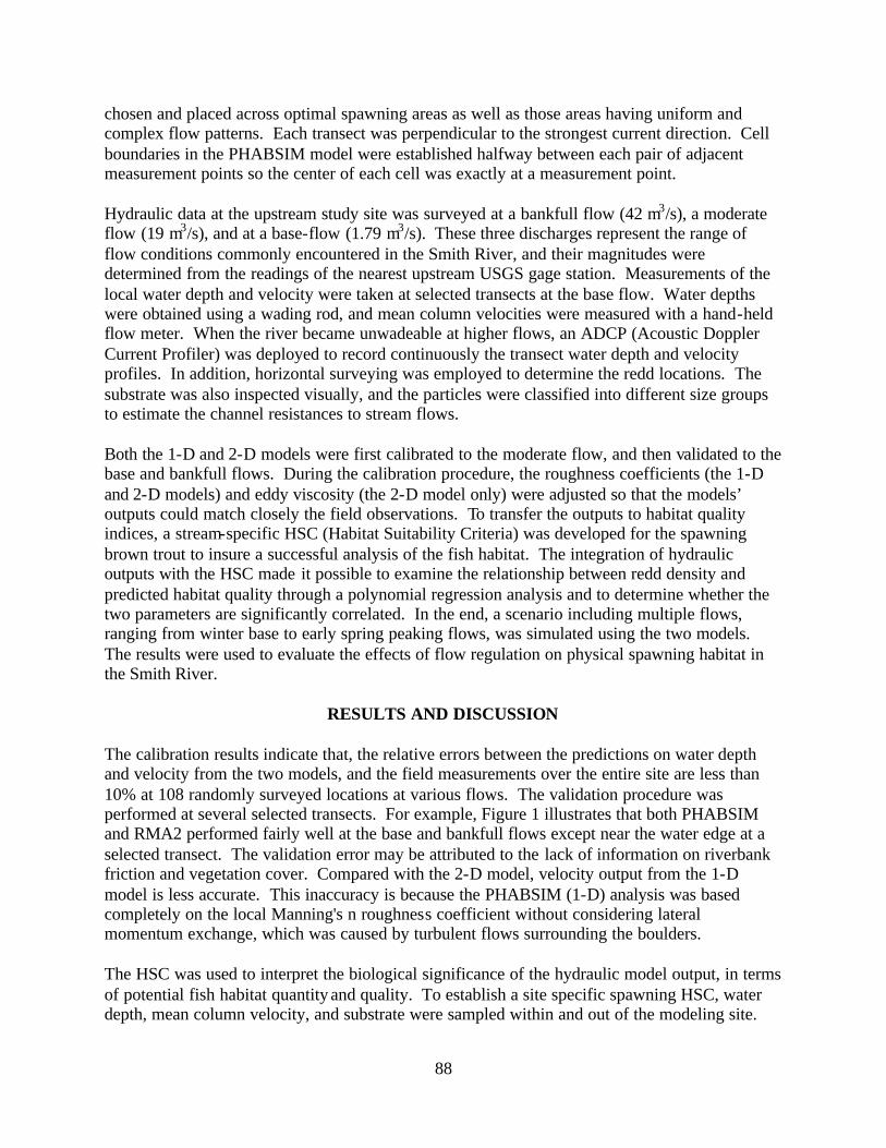
88

chosen and placed across optimal spawning areas as well as those areas having uniform and complex flow patterns. Each transect was perpendicular to the strongest current direction. Cell boundaries in the PHABSIM model were established halfway between each pair of adjacent measurement points so the center of each cell was exactly at a measurement point. Hydraulic data at the upstream study site was surveyed at a bankfull flow (42 m3/s), a moderate flow (19 m3/s), and at a base-flow (1.79 m3/s). These three discharges represent the range of flow conditions commonly encountered in the Smith River, and their magnitudes were determined from the readings of the nearest upstream USGS gage station. Measurements of the local water depth and velocity were taken at selected transects at the base flow. Water depths were obtained using a wading rod, and mean column velocities were measured with a hand-held flow meter. When the river became unwadeable at higher flows, an ADCP (Acoustic Doppler Current Profiler) was deployed to record continuously the transect water depth and velocity profiles. In addition, horizontal surveying was employed to determine the redd locations. The substrate was also inspected visually, and the particles were classified into different size groups to estimate the channel resistances to stream flows. Both the 1-D and 2-D models were first calibrated to the moderate flow, and then validated to the base and bankfull flows. During the calibration procedure, the roughness coefficients (the 1-D and 2-D models) and eddy viscosity (the 2-D model only) were adjusted so that the models’ outputs could match closely the field observations. To transfer the outputs to habitat quality indices, a stream-specific HSC (Habitat Suitability Criteria) was developed for the spawning brown trout to insure a successful analysis of the fish habitat. The integration of hydraulic outputs with the HSC made it possible to examine the relationship between redd density and predicted habitat quality through a polynomial regression analysis and to determine whether the two parameters are significantly correlated. In the end, a scenario including multiple flows, ranging from winter base to early spring peaking flows, was simulated using the two models. The results were used to evaluate the effects of flow regulation on physical spawning habitat in the Smith River.

RESULTS AND DISCUSSION

The calibration results indicate that, the relative errors between the predictions on water depth and velocity from the two models, and the field measurements over the entire site are less than 10% at 108 randomly surveyed locations at various flows. The validation procedure was performed at several selected transects. For example, Figure 1 illustrates that both PHABSIM and RMA2 performed fairly well at the base and bankfull flows except near the water edge at a selected transect. The validation error may be attributed to the lack of information on riverbank friction and vegetation cover. Compared with the 2-D model, velocity output from the 1-D model is less accurate. This inaccuracy is because the PHABSIM (1-D) analysis was based completely on the local Manning's n roughness coefficient without considering lateral momentum exchange, which was caused by turbulent flows surrounding the boulders.

The HSC was used to interpret the biological significance of the hydraulic model output, in terms of potential fish habitat quantity and quality. To establish a site specific spawning HSC, water depth, mean column velocity, and substrate were sampled within and out of the modeling site.

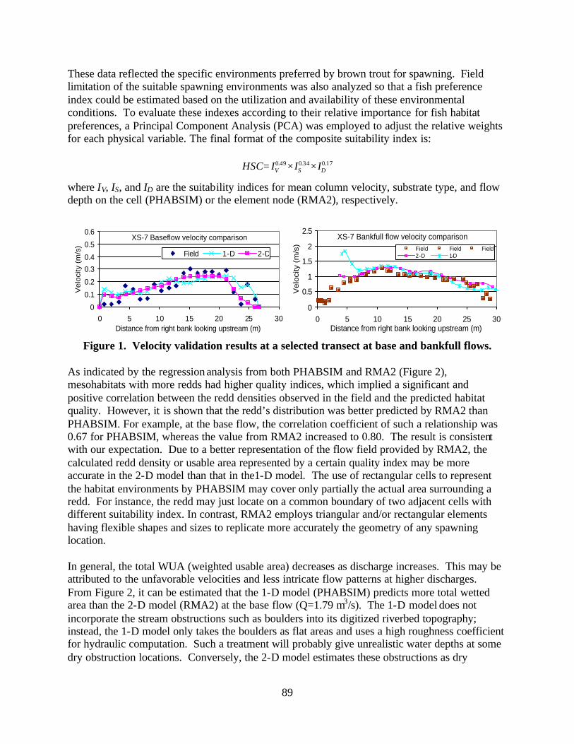
89

These data reflected the specific environments preferred by brown trout for spawning. Field limitation of the suitable spawning environments was also analyzed so that a fish preference index could be estimated based on the utilization and availability of these environmental conditions. To evaluate these indexes according to their relative importance for fish habitat preferences, a Principal Component Analysis (PCA) was employed to adjust the relative weights for each physical variable. The final format of the composite suitability index is:

17.034.049.0DSV IIIHSC ××=

where IV, IS, and ID are the suitability indices for mean column velocity, substrate type, and flow depth on the cell (PHABSIM) or the element node (RMA2), respectively.

Figure 1. Velocity validation results at a selected transect at base and bankfull flows.

As indicated by the regression analysis from both PHABSIM and RMA2 (Figure 2), mesohabitats with more redds had higher quality indices, which implied a significant and positive correlation between the redd densities observed in the field and the predicted habitat quality. However, it is shown that the redd’s distribution was better predicted by RMA2 than PHABSIM. For example, at the base flow, the correlation coefficient of such a relationship was 0.67 for PHABSIM, whereas the value from RMA2 increased to 0.80. The result is consistent with our expectation. Due to a better representation of the flow field provided by RMA2, the calculated redd density or usable area represented by a certain quality index may be more accurate in the 2-D model than that in the1-D model. The use of rectangular cells to represent the habitat environments by PHABSIM may cover only partially the actual area surrounding a redd. For instance, the redd may just locate on a common boundary of two adjacent cells with different suitability index. In contrast, RMA2 employs triangular and/or rectangular elements having flexible shapes and sizes to replicate more accurately the geometry of any spawning location. In general, the total WUA (weighted usable area) decreases as discharge increases. This may be attributed to the unfavorable velocities and less intricate flow patterns at higher discharges. From Figure 2, it can be estimated that the 1-D model (PHABSIM) predicts more total wetted area than the 2-D model (RMA2) at the base flow (Q=1.79 m3/s). The 1-D model does not incorporate the stream obstructions such as boulders into its digitized riverbed topography; instead, the 1-D model only takes the boulders as flat areas and uses a high roughness coefficient for hydraulic computation. Such a treatment will probably give unrealistic water depths at some dry obstruction locations. Conversely, the 2-D model estimates these obstructions as dry

XS-7 Bankfull flow velocity comparison

0

0.5

1

1.5

2

2.5

0 5 10 15 20 25 30Distance from right bank looking upstream (m)

Vel

ocity

(m

/s)

Field Field Field2-D 1-D

XS-7 Baseflow velocity comparison

0

0.1

0.2

0.3

0.4

0.5

0.6

0 5 10 15 20 25 30Distance from right bank looking upstream (m)

Vel

ocity

(m

/s)

Field 1-D 2-D

90

Figure 2. Habitat quality (left side) and quantity (right side) predicted at various flows (Q). WUA = weighted usable area. elements under low flow conditions and excludes them from the habitat calculation. This estimated result of the 2-D model is consistent with our field observations. Another advantage of the 2-D over the 1-D model is that PHABSIM underestimated the total WUA compared with the results from RMA2, except at the base flow. At the moderate flow (Q=19 m3/s), the WUA to total wetted area ratio predicted by the 1-D model is 45.29%, whereas the value computed by the 2-D model increases to 52.79%. This discrepancy comes from the shallow water areas. PHABSIM only considers the rectangle cell-averaged velocity and depth, which unavoidably exaggerates these values along the water edges. In contrast, the finite element mesh in the 2-D model can be adjusted to adapt to the highly irregular channel boundaries. The nodes can be setup along the banks and island edges, and the corresponding flow values on these nodes can be estimated independently from other nodes in deeper water.

CONCLUSIONS

Numerical results show that both the 1-D and 2-D models perform reasonably well in predicting water depth, velocity distribution, and fish habitat; but the 1-D model tends to underestimate the total WUA at high discharges. Significant and positive relationships between brown trout redd density and habitat quality indices are found through a regression analysis based on modeling simulations and field observations. It is concluded that, compared with the 1-D model, the 2-D method may allow a better representation of the physical environment of the fish habitat.

ACKNOWLEDGMENTS

We highly appreciate Donald Orth, Tammy Newcomb, Doug Novinger, Colin Krause and others from the Department of Fisheries and Wildlife Sciences at Virginia Tech for technical and field support.

REFERENCES

Relationship between Habitat Quality and redds density

1-D r = 0.67

2-D r = 0.80

0

0.005

0.01

0.015

0.02

0.025

0.03

0 0.1 0.2 0.3 0.4 0.5 0.6 0.7 0.8 0.9 1Suitability Index

2-D 1-DPoly. (1-D) Poly. (2-D)

Model Q

(cms) Wetted

Area(m2) WUA(m2)

WUA /Area(%

) 1.79 4360.03 2041.09 46.81

19 4629.11 2096.74 45.29 1-D

42 4629.11 841.74 18.18 1.79 4151.21 2039.55 49.1 19 4600.32 2428.31 52.79 2-D 42 4633.61 1011.71 21.8

Red

ds D

ensi

ty (p

er s

q m

eter

)

91

Bovee, K.D. 1982. A guide to stream habitat analysis using the Instream Flow Incremental Methodology. In: Instream Flow Information Paper, 12. U.S.D.I. Fish and Wildlife Service, Office of Biological Services FWS/OBS-82/26. 248 pp. Cochran, B. 1975. Best brown trout stream in the country. Virginia Wildlife 36(8): 16-17. Crowder, D.W. and P. Diplas. 2000. Evaluating spatially explicit metrics of stream energy gradients using hydrodynamic model simulations. Can. J. Fish. Aquat. Sci. 57: 1497-1507. King, I.P. 1990. Program documentation RMA2. Two dimensional finite element model for flow in estuaries and streams, Version 4.3. Resource Management Associate. Calif.

92

INVESTIGATION OF THE APPLICABILITY OF NEURAL-FUZZY LOGIC MODELING FOR CULVERT HYDRODYNAMICS

Jonathan M. Lester and Robert N. Eli

West Virginia University P.O. Box 6103, Morgantown, WV 26506

lesterjm@cox.net

KEY WORDS: neural- fuzzy logic, culverts, hydrodynamic modeling

ABSTRACT As a result of an earlier West Virginia Department of Highway study, the idea came to the forefront of using a completely new approach to analyzing the complex subject of culvert hydrodynamics. The literature indicates that there have been no reports of artificial intelligence, to include neural networks, fuzzy logic, or combined neural- fuzzy logic, used to investigate and predict culvert hydrodynamics. The scope of this research was to investigate the applicability of using neural- fuzzy logic to predict culvert diameters. To analyze these flows, commercial culvert software was employed to account for all types of flow conditions. This included different slopes, lengths, flow-rates, pipe sizes, and headwater and tailwater conditions. For all of the variables included in the analysis of culvert flow, some are complex in nature and require selection of different parameters. A large data set was created, from which to draw out different flow types for analysis. The use of fuzzy logic enables the user to enter variables, and the developed code then interprets the data and solves for diameter. These trained data sets have a complement checking data that is derived from similar calculations, with one variable slightly larger. These data sets were trained in a neural- fuzzy model, and the result was a predicted culvert diameter data set. The predicted diameters were then compared to the actual diameters to determine the accuracy of the model. For all data sets evaluated, the root mean square error was less than 12 inches. The overall weighted root mean squared error for the training data sets was 1.989 inches and 2.658 inches for the checking data sets.

INTRODUCTION

The Portland Cement Association (PCA) developed culvert capacity charts as early as 1962. Since their inception, many charts, nomographs, graphical solutions, and computer algorithms, have presented approximate predictions of the flow regime in a circular pipe. The Federal Highway Administration (FHWA) presented a working document in 1985, using charts and nomographs, to accommodate an analysis of flow capacity in culverts. Still more researchers have presented computer models to predict flow behavior in culverts. These works were a direct result of the complex nature of the flow through a culvert. The West Virginia Department of Highways convened a study to determine the methods to evaluate culverts that are greater that five hundred feet in length, which is the maximum length supported in their drainage manual. As a result of that study, the idea came to the forefront of us ing a completely new approach for analyzing this complex subject.

93

The literature indicates that there have been no reports of artificial intelligence, to include neural networks, fuzzy logic, or combined neural- fuzzy logic, used to investigate and predict culvert hydrodynamics. The purpose of the present work is to investigate the feasibility of using a neural- fuzzy logic model to predict culvert diameters. This function investigation is to determine if the neural- fuzzy logic model can be used to determine culvert size based on other input parameters.

METHOD The software selected to utilize Fuzzy Logic was MatLab from Math Works, Inc. Part of the MatLab package is the toolbox function: Adaptive Neural-Fuzzy Inference System (ANFIS). This powerful tool takes a given input and output data set and constructs a Fuzzy Inference System (FIS) who’s Membership Functions (MF) are adjustable. This function allows the fuzzy system to learn from the data it is modeling. In order to generate the data for use in training and checking the fit of the present neural- fuzzy logic model, the software Culvert Master, version 2.0 from Haestad Methods, was employed to calculate the headwater–discharge relationships. Haestad Methods required inputs of diameter, length, slope, headwater, and tailwater to calculate discharge. To achieve results from as broad a spectrum as possible, the culvert diameters varied from 24 inches to 96 inches, incrementing by 12 inches. These seven diameters were the basis for the training data set that was produced. In addition to the variance in diameter, the headwater depth varied from zero to 20 feet, in two-foot increments. The tailwater depth values ranged from zero to nine feet using one-foot increments. The values for length were 100, 250, 500, 750 and 1000 feet. These values of length caused the slope to vary according to the difference in elevation between the upstream invert and the downstream invert, ∆z. Values of ∆z were -0.1, -0.5, and -1.0 feet. Haestad Methods allows the user to increment the headwater in two-foot increments, which allowed eleven calculations at a time. Inputs of diameter, length, tailwater, and ∆z, the calculated slopes, plus a range of headwaters, produced a set of eleven discharges. This process was repeated, for all iterations, until the data set was complete. There were 11,550 lines of data in the data set, each one corresponding to a particular unique culvert flow condition. In addition to this training data set, there had to be a set of data that was used as the checking data. This latter data set was computed by offsetting the diameter by six inches. The purpose of providing checking data is to prevent the ANFIS from over training. The checking data used also served as a validation of goodness of fit of the particular ANFIS model. These offset diameters began at 30 inches and increased in increments of twelve inches until reaching a maximum diameter of 102 inches. This checking data set was computed in the same manner as the training data set, but assigned a different file name. Table 1 shows the constraints of the input variables used to compile the data sets. In the end, this process was repeated 2,100 times to complete the entire training and checking data sets. These data were then exported into an Excel spreadsheet, which was then used to sort the data into columnar format, so that it could be exported as a text data file, for loading into the ANFIS editor.

94

Table 1. Range of input values for compilation of culvert data. Variable Diameter (in) Length (ft) Headwater (ft) Tailwater (ft) Slope Range 24 – 102 100 – 1000 0 – 20 0 – 9 0.0001 – 0.01

As already explained, the slope varied according to a relationship between length and difference in elevation. The range of slopes is derived from the difference in upstream and downstream inverts, ∆z, using the three values -0.1, -0.5 and -1 feet. A progression of complexity was introduced by using four separate representative data sets. The step1 data set had three variables; headwater (HW), discharge (Q), and diameter (D). The tailwater (TW), slope (So) and length (L) were held constant at arbitrarily selected values. The step 2 data set had four variables: headwater, discharge, diameter, and tailwater—holding slope and length constant. The step 3 data set had five variables: headwater, discharge, diameter, tailwater slope—holding only the length constant. The final step, step 4, includes all six variables. Table 2 below summarizes the four different data sets, the variables held and varied, as well as the file size.

Table 2. Progression of variable complexity showing corresponding row and column size for different data sets.

Step Hold Vary Rows Columns 1 So = 0.004, L = 250’, TW = 2’ HW, Q, D 77 3 2 So = 0.004, L = 250’ HW, Q, TW,D 770 4 3 L = 250’ HW, Q, TW, So, D 2,310 5 4 N/A HW, Q, TW, So, L, D 11,550 6

In order to describe the flow regime for a particular culvert, there are several variables that must be taken into account. Culverts can be generally described based on inlet or outlet control. According to Chow (1959) and the United States Geological Survey (1976), they can be further broken down into six different types. These different types were used to separate the data generated, and each was analyzed separately according to type. The representative data for each type was extracted from the total data set, according to the constraints associated with that particular type. This process provided a more detailed analysis for comparison purposes. The different types are summarized and illustrated in Figure 1.

RESULTS AND DISCUSSION In order to determine how well the model fits the computed data, the ANFIS editor reports the epoch error as well as the checking error. Additionally, the use of a root mean squared error (RMSE) was utilized. Table 3 is arranged in chronological order. The first two rows are the results for type 4 and 5, which were solved explicitly. Both the step data sets and the six types were generated using code. The step data sets are presented in the center of the table. Finally the six different culvert types are presented at the bottom of the table. These results were better than the step data sets and gave very similar accuracies for type 4 and type 5 that were solved explicitly. These results are the error above or below the expected result, in inches, that were tabulated from results of each MatLab model run and the corresponding RMSE calculations.

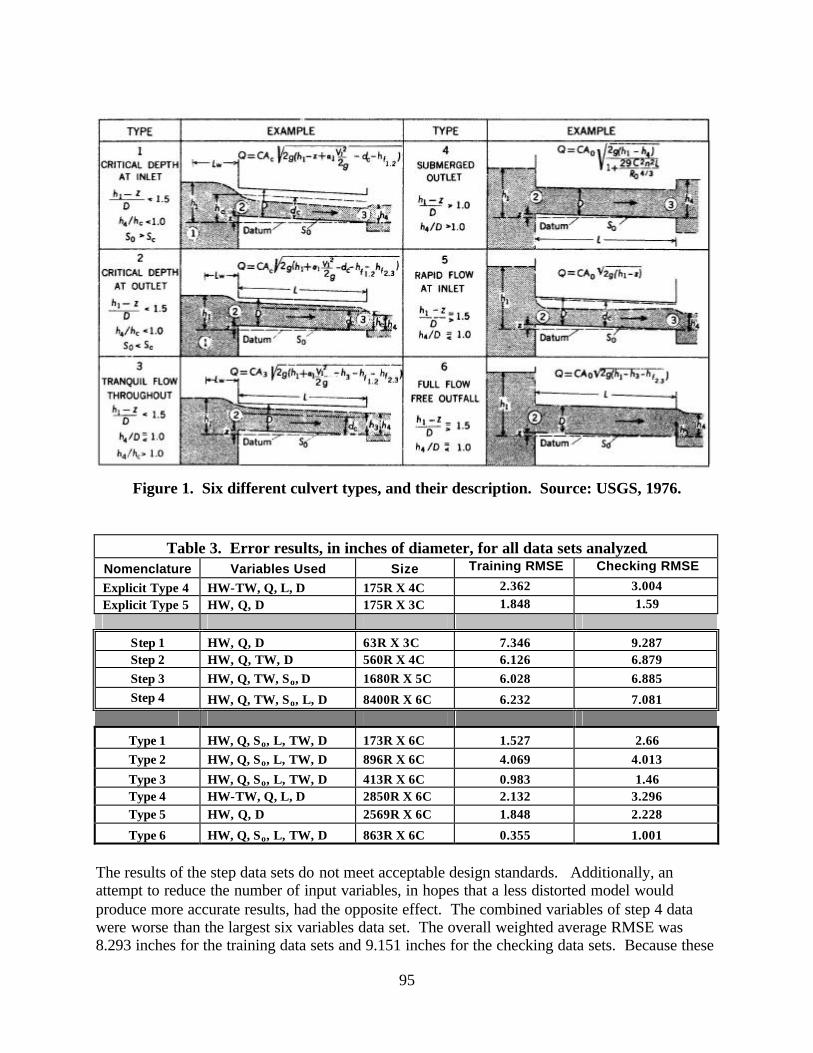
95

Figure 1. Six different culvert types, and their description. Source: USGS, 1976.

Table 3. Error results, in inches of diameter, for all data sets analyzed. Nomenclature Variables Used Size Training RMSE Checking RMSE

Explicit Type 4 HW-TW, Q, L, D 175R X 4C 2.362 3.004 Explicit Type 5 HW, Q, D 175R X 3C 1.848 1.59

Step 1 HW, Q, D 63R X 3C 7.346 9.287 Step 2 HW, Q, TW, D 560R X 4C 6.126 6.879 Step 3 HW, Q, TW, So, D 1680R X 5C 6.028 6.885 Step 4 HW, Q, TW, So, L, D 8400R X 6C 6.232 7.081

Type 1 HW, Q, So, L, TW, D 173R X 6C 1.527 2.66 Type 2 HW, Q, So, L, TW, D 896R X 6C 4.069 4.013

Type 3 HW, Q, So, L, TW, D 413R X 6C 0.983 1.46 Type 4 HW-TW, Q, L, D 2850R X 6C 2.132 3.296 Type 5 HW, Q, D 2569R X 6C 1.848 2.228

Type 6 HW, Q, So, L, TW, D 863R X 6C 0.355 1.001 The results of the step data sets do not meet acceptable design standards. Additionally, an attempt to reduce the number of input variables, in hopes that a less distorted model would produce more accurate results, had the opposite effect. The combined variables of step 4 data were worse than the largest six variables data set. The overall weighted average RMSE was 8.293 inches for the training data sets and 9.151 inches for the checking data sets. Because these

96

results were not acceptable, the six type data sets were analyzed in order to obtain more accurate results. In order to quantify the error results, the fact that culvert designers are not looking for an exact numerical diameter, but the nearest approximate standard diameter for a specified geometry and flow rate combination, has been taken into consideration. With this in mind, the results were bracketed into six inches above the actual diameter and six inches below the actual diameter, which corresponds to the mid-point between standard pipe sizes. Therefore, if the data fell into this range of predicted diameters, they were rounded to the nearest standard pipe size. This process creates permissible error bounds for the data about each standard pipe diameter.

The results of all the data sets are presented in terms of what percent fell outside of the error bounds. The optimal result would be zero falling outside the error bounds. Table 4 shows the data sets and their respective percent falling outside of the error bounds, for step 1 through 4 data sets. The high percentages falling outside the error bounds correspond to the higher error results presented in Table 3.

Table 4. Percent of data points falling outside of error bounds for step data sets.

Nomenclature Training, % outside Checking, % outside Step 1 28.570 47.620 Step 2 18.570 17.500 Step 3 18.210 17.740 Step 4 17.96 18.35

The results obtained with the six culvert type data sets were also analyzed to determine how well they fit the error bounds. Table 5 below lists the results of this error bound analysis. Type 2 results were the worst, of all six types analyzed; however, more than 90 percent were within the error bounds, which is acceptable for culvert design.

Table 5. Percent of data points falling outside error bounds for six culvert types.

Nomenclature Training, % outside Checking, % outside Type 1 0.00 2.89 Type 2 6.47 9.30 Type 3 0.00 0.24 Type 4 0.00 0.00 Type 5 0.74 2.34 Type 6 0.00 0.58

97

CONCLUSIONS

Since culvert designers utilize an approach that rounds to the next highest pipe size, it is believed that the use of a neural- fuzzy logic model is acceptable for predicting culvert diameters. These results were, however, based on concrete culvert pipe with a standard entrance loss coefficient. Initial results of ANFIS application to the formula generated Type 4 and 5 data sets revealed root mean square errors ranging between 1.5 and 3 inches. This fell into the acceptable design criteria for culverts. Using similar explicit solutions for the other four types proved too difficult, time consuming, and with questionable accuracy; therefore, an alternate method of calculating data to analyze was sought. The decision to use Haestad Methods – CulvertMaster software was made based on the capability with Hydraulic Design of Highway Culverts (Normann, et al. 1985). This software produced results that were not classified according to the types, thus an intricate conditional if-then logic structure was employed to separate the large data set into the six different culvert types. Given the less than acceptable results from the four step data sets, the six different culvert types (Figure 1) were analyzed to determine if the breakdown of data sets by culvert classification would produce better results. From the RMSE data, listed in Table 3, it can be concluded that the error ranges from one inch to four inches. To put this error in perspective, if a 24- inch diameter culvert was predicted and the error was as much as four inches, this error would be seventeen percent. This error is unacceptable by the standards used in culvert design. On the other end of the spectrum, if a 96- inch diameter culvert was predicted and the error was as much as four inches, the error would be less than five percent. This latter error, by standards acceptable to most all culvert designers, would fall into the acceptable category. When designing culverts, the purpose is to determine the diameter needed to pass the design flow-rate for the culvert geometry provided. This answer is then rounded up to the next available standard pipe size. In order to reduce manufacturing costs, standard pipe sizes have been adopted, thus reducing the higher cost of producing a uniquely sized pipe. With this approach in mind, the results were placed into a band of six inches above the actual diameter and six inches below the actual diameter, which is the halfway point between the standard diameters. This process reduced the effective error, by placing more than 70 percent of the predicted diameters within the acceptable error band about each standard diameter. This study explored the application of neural- fuzzy logic models to the culvert design problem for the first time. It was originally intended that the neural- fuzzy model be fitted to the culvert performance data without separation by flow regime classification; however, the predictive errors on diameter where too large to be acceptable for use as a design tool. It is possible that alternate approaches to the application of the neural- fuzzy model could result in more acceptable results with the combined data set. It is recommended that additional studies be conducted to explore the possibility of other optimal structures of number and type of membership functions used in the ANFIS model. It is possible that there are undiscovered model structures that will reduce the error to acceptable levels.

98

Additionally, it is recommended that the applicability of a neural network modeling approach be investigated, since this study shows that the neural network component of the neural- fuzzy logic model had some success in mapping the input to output data relationship. It is possible that a neural network, used alone, can perform better in mapping the input data to the output culvert diameter. For a more thorough analysis of all culverts possible, the study should be broadened into different pipe material and entrance conditions, as well as a much broader range of bed slope values.

ACKNOWLEDGMENTS

The authors would like to express their appreciation for the countless number of people who provided assistance over the past few years in making this research come to fruition.

REFERENCES Chow, V.T. 1959. Open Channel Hydraulics. McGraw-Hill. New York, N.Y. Normann, J.M., R.J. Haughtalen, and W.J. Johnston. 1985. Hydraulic Design of Highway Culverts. Report No. FHWA-IP-85-15, Federal Highway Administration. McLean, Va. United States Geological Survey. 1976. Measurement of Peak Discharge at Culverts by Indirect Methods. Book 3, Chapter A3.

99

SOURCES OF FECAL POLLUTION IN WASHINGTON D.C. WATERWAYS

Kim Porter and Charles Hagedorn Virginia Tech

401 Price Hall, Blacksburg VA 24061 kporter@vt.edu

KEY WORDS: bacterial source tracking, Enterococcus, antibiotic resistance analysis

ABSTRACT Fecal pollution of major waterways in the Washington D.C. area is a substantial recreational use issue and health concern. The objective of this project was to identify the sources of fecal pollution via bacterial source tracking in three major waterways: Rock Creek, the Anacostia River, and the Potomac River. Over the sampling period, two dominant sources of fecal pollution were detected in the Potomac River, three dominant sources were detected in Rock Creek, and one dominant source was detected in the Anacostia River. The impact of human fecal pollution is substantial in all three waterways, especially during the dry summer months.

INTRODUCTION The microbiological quality of our nation’s waters is a topic of great concern and intense research. In 2000, the latest report from the National Water Quality Inventory report was published reporting approximately 40% of streams, 45% of lakes, and 51% of estuaries were not clean enough to support recreational uses such as fishing and swimming. The leading cause of impairment to the rivers and streams is pathogenic microbes (EPA 2002). The microbiological maintenance of waters that have primary or secondary human contact is imperative, as contamination can create serious health risks. Establishing the source of fecal contamination is crucial for the evaluation of health risks as well as for the direction of remediation efforts. In 1996, the District of Columbia developed a list of waters that did not meet state water quality standards that was submitted to the EPA for inclusion on the 303(d) list as required by the Clean Water Act. For all impaired waters listed across the state, a Total Maximum Daily Load (TMDL) report must be developed to estimate all significant sources of a pollutant, the specific amount coming from each source, and the reduction needed to bring the impaired body of water back into compliance with the water quality standards (Kern et al. 2002). This study will aid the Metropolitan Washington Council of Governments (MWCOG) in the creation of a TMDL report for fecal coliform exceedance in Rock Creek, the Anacostia River, and the Potomac River. The initial sources of fecal contamination were thought to be combined sewer overflows, stormwater runoff, direct deposits of feces into the water from wildlife, and separate sanitary sewer overflows that can result from leaky or undersized sanitary sewer pipes (Department of Health et al. 2002). The highest level of concern stems from the city’s current combined sewer system. According to The Washington Post, approximately 75 times a year, the system becomes overloaded and then flows into emergency pipes where it mixes with sewage from the Blue

100

Plains sewage treatment facility (Vasquez 2002). The emergency pipes empty the sewage/stormwater mixture directly into the Potomac River, the Anacostia River, and Rock Creek. This amounts to roughly three billion gallons of unprocessed wastewater discharge into these waterways annually. Most source tracking projects completed in the past have been for rural watersheds. This project is unique in that it is one of the first major source tracking projects attempting to assess fecal contamination sources in a major metropolitan area. The introduction of fecal matter and human pathogens into the water has the potential to impact a large population because these waterways are major recreational sites. The results of this project have a wide reaching impact for the Washington D.C. area, which may include the need for a complete renovation of the current combined sewer system.

METHODS A known source fecal bacteria library profile was created, consisting of 1,806 Enterococcus isolates from known sources including human, cattle, chicken, horse, goat, sheep, deer, raccoon, muskrat, goose, seagull, coyote, duck, wild turkey, dog, and cat. Each known source Enterococci isolate was evaluated using Antibiotic Resistance Analysis (ARA) for growth on thirty concentrations of nine antibiotics and either growth (1) or no growth (0) was recorded for each isolate at each concentration. This pattern of growth/no growth formed the antibiotic resistance profile for each Enterococci isolate. The isolate profiles were then combined to form the known source libraries. The library was analyzed using logistic regression. Monthly sampling was completed on six locations along Rock Creek, six locations along the Anacostia River, and three locations along the Potomac River from July 2002 through May 2003, with additional sampling after two major storm events. The Enterococci in the water samples from each month were isolated using membrane filtration. ARA of the isolates was used to create patterns that were run against the known isolate profile library to determine the proportion of isolates from the sources of bird, horse, human, livestock, pets, and wildlife.

RESULTS AND DISCUSSION To account for localized sources of fecal contamination, a known source library was established for each waterway. The Rock Creek library was divided into a five-way (Bird, Horse, Human, Pets, and Wildlife) classification with an Average Rate of Correct Classification (ARCC) of 92.7%. The Anacostia River library was divided into a four-way (Bird, Human, Pets, and Wildlife) classification with an ARCC of 93.0%. The Potomac River library was divided into a five-way (Bird, Human, Livestock, Pets, and Wildlife) classification with an ARCC of 88.6%. The ARA results of the unknown stream isolates for all three waterways were analyzed to determine the dominant sources of contamination based on a ten-month average. The ARA results were also used to study the effect of storm events on source distributions and seasonal variation patterns. The averages are presented in Table 1. The dominant sources of fecal contamination detected in each waterway varied by site, season, and storm events. Horse, human, and wildlife were the dominant sources found in Rock Creek. The dominant source in

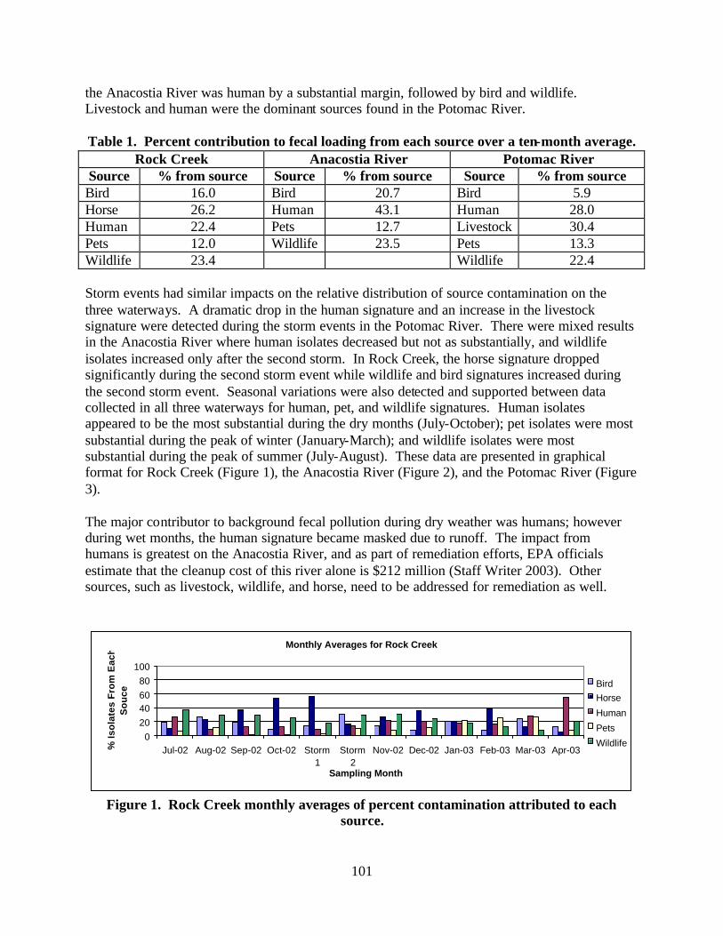
101

the Anacostia River was human by a substantial margin, followed by bird and wildlife. Livestock and human were the dominant sources found in the Potomac River. Table 1. Percent contribution to fecal loading from each source over a ten-month average.

Rock Creek Anacostia River Potomac River Source % from source Source % from source Source % from source Bird 16.0 Bird 20.7 Bird 5.9 Horse 26.2 Human 43.1 Human 28.0 Human 22.4 Pets 12.7 Livestock 30.4 Pets 12.0 Wildlife 23.5 Pets 13.3 Wildlife 23.4 Wildlife 22.4 Storm events had similar impacts on the relative distribution of source contamination on the three waterways. A dramatic drop in the human signature and an increase in the livestock signature were detected during the storm events in the Potomac River. There were mixed results in the Anacostia River where human isolates decreased but not as substantially, and wildlife isolates increased only after the second storm. In Rock Creek, the horse signature dropped significantly during the second storm event while wildlife and bird signatures increased during the second storm event. Seasonal variations were also detected and supported between data collected in all three waterways for human, pet, and wildlife signatures. Human isolates appeared to be the most substantial during the dry months (July-October); pet isolates were most substantial during the peak of winter (January-March); and wildlife isolates were most substantial during the peak of summer (July-August). These data are presented in graphical format for Rock Creek (Figure 1), the Anacostia River (Figure 2), and the Potomac River (Figure 3). The major contributor to background fecal pollution during dry weather was humans; however during wet months, the human signature became masked due to runoff. The impact from humans is greatest on the Anacostia River, and as part of remediation efforts, EPA officials estimate that the cleanup cost of this river alone is $212 million (Staff Writer 2003). Other sources, such as livestock, wildlife, and horse, need to be addressed for remediation as well.

Monthly Averages for Rock Creek

020406080

100

Jul-02 Aug-02 Sep-02 Oct-02 Storm1

Storm2

Nov-02 Dec-02 Jan-03 Feb-03 Mar-03 Apr-03

Sampling Month

% Is

ola

tes

Fro

m E

ach

S

ou

ce

BirdHorse

Human

Pets

Wildlife

Figure 1. Rock Creek monthly averages of percent contamination attributed to each

source.

102

Monthly Averages for the Anacostia River

0

20

40

60

80

100

Jul-02 Aug-02 Sep-02 Oct-02 Storm 1 Storm 2 Nov-02 Dec-02 Jan-03 Feb-03 Mar-03 Apr-03Sampling Month

% Is

olat

es F

rom

E

ach

Sou

rce Bird

Human

Pets

Wildlife

Figure 2. Anacostia River monthly averages of percent contamination attributed to each

source.

Monthly Averages for the Potomac River

020406080

100

Jul-02 Aug-02 Sep-02 Oct-02 Storm1

Storm2

Nov-02 Dec-02 Jan-03 Feb-03 Mar-03 Apr-03

Sampling Month

% Is

ola

tes

Fro

m

Eac

h S

ou

rce Bird

Human

LivestockPets

Wildlife

Figure 3. Potomac River monthly averages of percent contamination attributed to each source.

ACKNOWLEDGMENTS There are many who deserve a big thanks for their help in various aspects of this project. First, I would like to thank my advisor Dr. Charles Hagedorn for his guidance. I would also like to thank my graduate committee, Dr. Tamim Younos and Dr. Carl Zipper. I would also like to thank MWCOG for the funding of this project, especially T.J. Murphy and Mukhtar Ibrahim and Harold Post (Field Operations Supervisor), and Doug, Phil, and Mark at the Occoquan Watershed Monitoring Lab who were responsible for organizing and carrying out sampling events.

REFERENCES Department of Health, Environmental Health Administration, Bureau of Environmental Quality, Water Quality Division, Water Quality Control Branch. August 2002. Total Maximum Daily Load, District of Columbia, Fecal Coliform. Unpublished Report. Environmental Protection Agency. 2002. Water Quality Conditions in the United States, A Profile from the 2000 National Water Quality Inventory. http://www.epa.gov/305b/2000report/factsheet.pdf (27 May 2003).

103

Kern, J., B. Petrauskas, P. McCelellan, V. Shanholtz, C. Hagedorn. 2002. Bacterial source tracking: A tool for Total Maximum Daily Load development. In: Advances in Water Monitoring Research. T. Younos (Editor). Water Resources Publication, LLC. Denver, Colo. pp. 125-142. Staff Writer. City gets money for Anacostia cleanup. The Washington Post. April 22, 2003. Section B4. Vasquez, M. A problem between rain and the rivers, city seeks U.S. funds to cut waste spillage. The Washington Post. August 15, 2002. Section J, p T3.

104

IMPACT OF LAND USE ON FECAL COLIFORM LEVELS IN SURFACE WATERS OF FAIRFAX COUNTY, VIRGINIA

Judith A. Buchino

Environmental Science and Policy, George Mason University 2231 Aryness Drive, Vienna, VA 22181

jbuchino@gmu.edu

KEY WORDS: land use, fecal coliforms, water quality, GIS

EXTENDED ABSTRACT The purpose of this research is to investigate the problem of fecal coliform levels in the surface waters of Fairfax County and to investigate the role of land use in explaining the problem. An in depth analysis of the Fairfax County Health Department monitoring data, both the fecal coliform data and the chemical parameter data, will elucidate the relationship between these elevated fecal coliforms and land use. This study will examine the countywide distribution of elevated levels of fecal coliform and correlate this with land use. This information will assist in the decision-making process in two areas of importance to Fairfax County: water quality management and land-use management. The conclusions will apply to decision-making processes in rapidly developing suburban regions similar to Northern Virginia.

INTRODUCTION

Fecal coliform contamination has been a persistent problem for surface water systems throughout the years. In 1885, the German bacteriologist Theodor Escherich discovered the bacterium that is characteristic of fecal contamination in water, Escherichia coli (Geldreich 1966, Madigan et al. 1997). Although not always disease producing themselves, fecal coliforms (FC) serve as an indicator organism for possible pathogens that are present in fecal material. Despite the great advances in wastewater treatment management, fecal coliform contamination is still persistent, especially in larger metropolitan regions. Sources of the fecal coliforms include human sewage attributable to failing septic systems, faulty wastewater treatment systems, domestic animals, farm animals, the use of manure on agricultural plots, and wildlife (Geldreich and Kenner 1969). The Fairfax County Health Department routinely collects surface water samples to monitor the quality of its streams and lakes. The county provides an excellent annual summary report: The Fairfax County 2000 Stream Water Quality Report that may be used in research to investigate the relationships among other environmental data sets, particularly land use, precipitation, and soil imperviousness. These resulting relationships will enlighten the community on the importance of land use and its potential impact on water quality.

105

METHODS The objective of this analysis is to evaluate the relationship between land use and the elevated fecal coliform levels in the surface waters of Fairfax County. There are thirty watersheds within the boundaries of Fairfax County, Virginia. They include Accotink Creek, Belle Haven, Bull Neck Run, Bull Run, Cameron Run, Cub Run, Dead Run, Difficult Run, Dogue Creek, Four Mile Run, High Point, Horsepen Creek, Johnny Moore Creek, Kane Creek, Little Hunting Creek, Little Rocky Run, Mill Branch, Nichol Run, Occoquan, Old Mill Branch, Pimmit Run, Pohick Creek, Pond Branch, Popes Head Creek, Ryans Dam, Sandy Run, Scotts Run, Sugarland Run, Turkey Run, and Wolf Run. The Fairfax County Public Health data are collected from 85 sampling sites in 25 of the 30 watersheds in Fairfax County. This research project consists of the following tasks:

1. Assembly of the database 2. Compilation of descriptive statistics 3. Investigation of explanatory models

The purpose of the database construction task was to build a spatially and temporally matched database with the water chemistry data set, the fecal coliform data set, and the latitude/longitude coordinates for the sampling sites. The database includes data from 1986–1999. GIS was used to relate land use by sub-watershed regions subdivided into segments for each sampling site. The percent of land use by category was calculated for each segment. This information was then exported from GIS into an EXCEL spreadsheet and was read into S-PLUS for further data analysis. Fairfax County currently has over 30 relevant GIS themes and attributes available. The Fairfax County GIS layers are stored in the datum, Virginia State Plane North NAD 83, and the units are feet. Land-use data from the Northern Virginia Regional Commission are also available. These land-use data combine 14 jurisdictional regions into one comprehensive GIS layer. The calculation of impervious surfaces was conducted using the technique developed by Fairfax County for the Stream Protection Strategy (SPS) report (2001). Details of this methodology are provided in Appendix F of the SPS report. Summary statistics were performed in S-PLUS 6.1. Analysis for outliers and extraneous values were conducted, and transformation of the data was made when necessary. The quantile-quantile plot, or Q-Q plot, compared the distributions of two or more sets of univariate measurements. Paired Q-Q plots are effective in comparing distributions by category of the variable. Box plots are another method for summarizing the distributions of a variable measured at different categories (Cleveland 1993). Exploratory data analysis is helpful in obtaining an overview of the data, and as an aid in determining whether the variables are normally (Gaussian) distributed, which is a key assumption made in using parametric statistical tests. If the data are not normally distributed, then non-parametric tests need to be conducted.

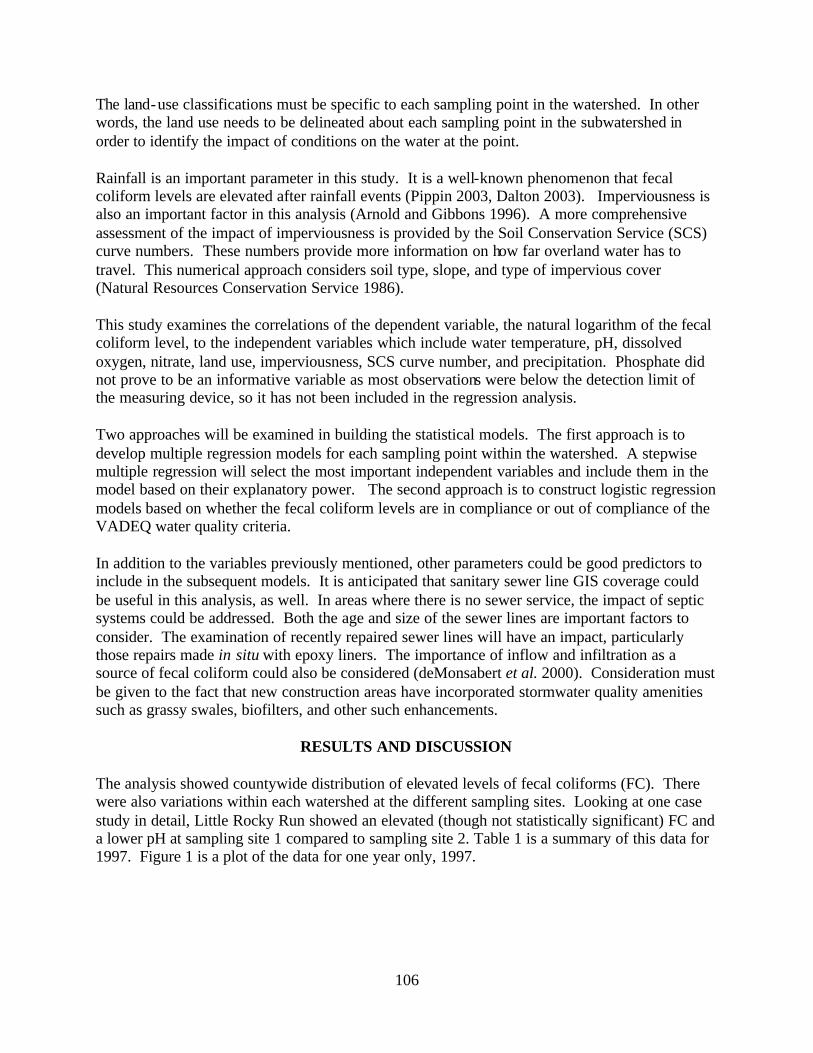
106

The land-use classifications must be specific to each sampling point in the watershed. In other words, the land use needs to be delineated about each sampling point in the subwatershed in order to identify the impact of conditions on the water at the point. Rainfall is an important parameter in this study. It is a well-known phenomenon that fecal coliform levels are elevated after rainfall events (Pippin 2003, Dalton 2003). Imperviousness is also an important factor in this analysis (Arnold and Gibbons 1996). A more comprehensive assessment of the impact of imperviousness is provided by the Soil Conservation Service (SCS) curve numbers. These numbers provide more information on how far overland water has to travel. This numerical approach considers soil type, slope, and type of impervious cover (Natural Resources Conservation Service 1986). This study examines the correlations of the dependent variable, the natural logarithm of the fecal coliform level, to the independent variables which include water temperature, pH, dissolved oxygen, nitrate, land use, imperviousness, SCS curve number, and precipitation. Phosphate did not prove to be an informative variable as most observations were below the detection limit of the measuring device, so it has not been included in the regression analysis. Two approaches will be examined in building the statistical models. The first approach is to develop multiple regression models for each sampling point within the watershed. A stepwise multiple regression will select the most important independent variables and include them in the model based on their explanatory power. The second approach is to construct logistic regression models based on whether the fecal coliform levels are in compliance or out of compliance of the VADEQ water quality criteria. In addition to the variables previously mentioned, other parameters could be good predictors to include in the subsequent models. It is anticipated that sanitary sewer line GIS coverage could be useful in this analysis, as well. In areas where there is no sewer service, the impact of septic systems could be addressed. Both the age and size of the sewer lines are important factors to consider. The examination of recently repaired sewer lines will have an impact, particularly those repairs made in situ with epoxy liners. The importance of inflow and infiltration as a source of fecal coliform could also be considered (deMonsabert et al. 2000). Consideration must be given to the fact that new construction areas have incorporated stormwater quality amenities such as grassy swales, biofilters, and other such enhancements.

RESULTS AND DISCUSSION

The analysis showed countywide distribution of elevated levels of fecal coliforms (FC). There were also variations within each watershed at the different sampling sites. Looking at one case study in detail, Little Rocky Run showed an elevated (though not statistically significant) FC and a lower pH at sampling site 1 compared to sampling site 2. Table 1 is a summary of this data for 1997. Figure 1 is a plot of the data for one year only, 1997.

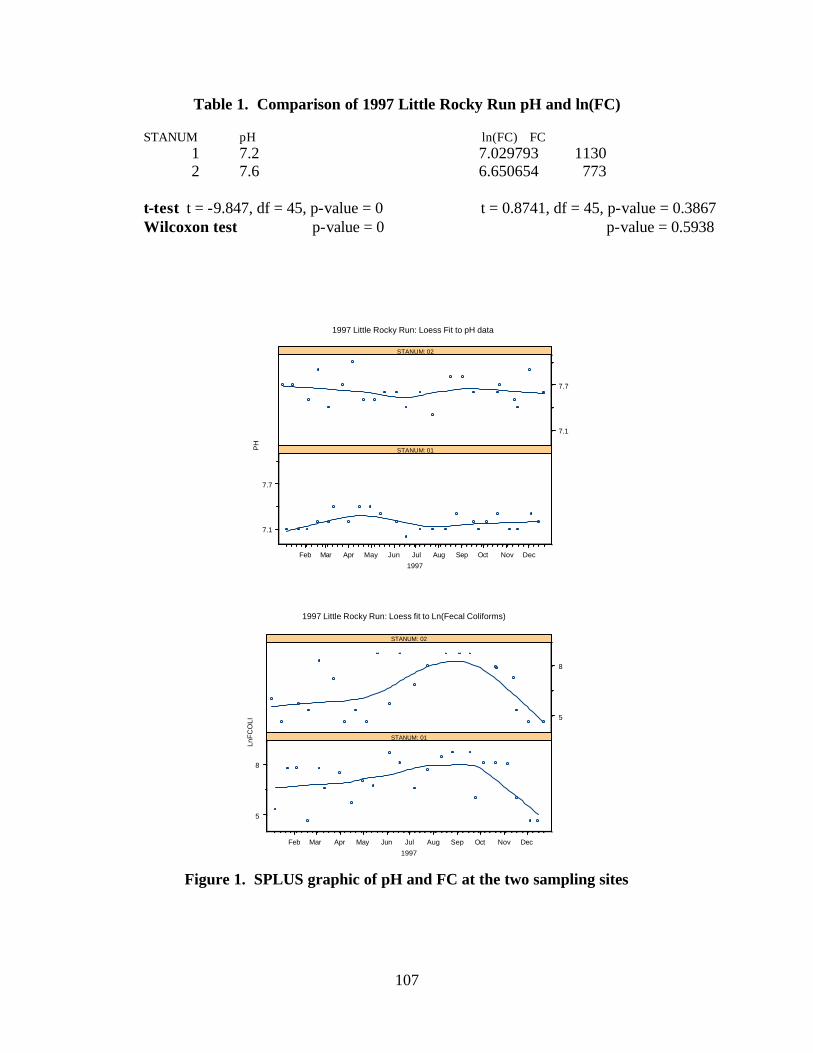
107

Table 1. Comparison of 1997 Little Rocky Run pH and ln(FC)

STANUM pH ln(FC) FC 1 7.2 7.029793 1130 2 7.6 6.650654 773

t-test t = -9.847, df = 45, p-value = 0 t = 0.8741, df = 45, p-value = 0.3867 Wilcoxon test p-value = 0 p-value = 0.5938

Feb Mar Apr May Jun Jul Aug Sep Oct Nov Dec

1997

7.1

7.7

7.1

7.7

PH

STANUM: 01

STANUM: 02

1997 Little Rocky Run: Loess Fit to pH data

Feb Mar Apr May Jun Jul Aug Sep Oct Nov Dec

1997

5

8

5

8

LnF

CO

LI

STANUM: 01

STANUM: 02

1997 Little Rocky Run: Loess fit to Ln(Fecal Coliforms)

Figure 1. SPLUS graphic of pH and FC at the two sampling sites

108

Although these values for pH fall within the range of “normal” limits, further work is needed to investigate the reason for this variation, specifically whether a difference in land use between the two sites could possibly account for this. The primary land use in Little Rocky Run is Low to Medium Density Residential, which comprises 80% of the land in sampling site 1 vs. 62% of the land in sampling site 2. The fecal coliform levels for Little Rocky Run are not statistically different between sampling site 1 and 2, although both values are above the geometric mean of 200 cfu/100ml.

FUTURE WORK

All twenty-five watersheds sampled will be investigated. Specific years will be stud ied based on the availability of land-use coverage. Formal hypothesis testing will be done to determine whether differences found in measured variables are statistically significant. Ramifications for ecological significance will be evaluated and discussed.

ACKNOWLEDGMENTS

The author would like to acknowledge assistance provided by Northern Virginia Regional Commission; Matt Handy, Laura Grape, Dipmani Kumar, Ed Pippin (Fairfax County); Asad Rouhi (Northern Virginia Soil and Water Conservation District); committee members, Dr. Sheryl Luzzadder Beach, Dr. R. Chris Jones, Dr. Sharon deMonsabert, Dr. Carol Litchfield, and Dr. Dan Carr (George Mason University). Additional assistance was given from Dr. David Wong and Dr. Long Chiu (George Mason University).

REFERENCES

Arnold, C. L. and C. J. Gibbons. 1996. Impervious surface coverage: the emergence of a key environmental indicator. Journal of the American Planning Association 62(2): 243-258. Cleveland, W. S. 1993. Visualizing Data. AT&T Bell Laboratories. Murray Hill, N. J. Dalton, C. 2003. Microbial source tracking in two southern Maine watersheds. http://www.umseagrant-mst.org/results_rain.htm (January 15, 2004). DeMonsabert. S., C. Ong, and P. Thornton. 2000. An integer program for optimization of sanitary sewer rehabilitation over a planning horizon. Water Environment Research Jan. Fairfax County 2000 Stream Water Quality Report. 2000. Fairfax County Health Department Division of Environmental Health. Fairfax, Va. http://www.fairfaxcounty.gov/service/hd/strannualrpt.htm (January 15, 2004). Fairfax County Stream Protection Strategy Baseline Study. 2001. Stormwater Planning Division, Department of Public Works and Environmental Services. Fairfax County, Va. http://www.co.fairfax.va.us/dpwes/environmental/SPS_pdf.htm (January 15, 2004).

109

Geldreich, E. E. 1966. Sanitary Significance of Fecal Coliforms in the Environment. U.S. Department of the Interior, Federal Water Pollution Control Administration. Cincinnati, Ohio. Geldreich, E. E. and B. A. Kenner. 1969. Concepts of fecal streptococci in stream pollution. Journal Water Pollution Control Federation 41: R336-R352. Madigan, M.T., J.M. Martinko, and J. Parker. 1997. Brock Biology of Microorganisms, Eighth edition. Prentice Hall. Upper Saddle River, N.J. Natural Resources Conservation Service, United States Department of Agriculture. 1986. Urban Hydrology for Small Watersheds, Technical Release 55. http://www.wcc.nrcs.usda.gov/hydro/hydro-tools-models.html (January 15, 2004). Pippin, E. L. 2003. Fairfax County Health Department. Personal communication.

110

FECAL COLIFORMS, E. COLI, AND HUMANS’ INFLUENCE ON SMITH MOUNTAIN LAKE

Carolyn L. Thomas and David M. Johnson

Ferrum College Box 1000, Ferrum, VA 24088

cthomas@ferrum.edu

KEY WORDS: water quality, fecal coliforms, E. coli, Smith Mountain Lake

INTRODUCTION

The Smith Mountain Lake Volunteer Water Quality Monitoring Program was initiated in 1987 and has functioned each year since. Smith Mountain Lake is a 25,000-acre pump-storage reservoir located in southwestern Virginia. The program monitors the trophic status of Smith Mountain Lake. Beginning in 1996, monitoring of fecal coliform bacteria has been carried out to assess the bacteriological quality of the water as well as the degree of nutrient enrichment.

METHODS

The samples were collected and stored according to standard methods (APHA 1995). The fecal coliform determination included a standard 100 mL-aliquot of sample, which was filtered immediately upon return to the laboratory. The membrane filtration method for bacterial analyses was used with DIFCO m-Fecal Coliform media prepared with rosolic acid, as prescribed in standard methods (APHA 1995). Characteristic blue fecal coliform colonies were counted and recorded after 22-24 hours of incubation at 45.5 °C in an incubator.

The Antibiotic Resistance Assay (ARA) method used was developed by Dr. Charles Hagedorn from Virginia Tech and his associates. The method is explained in Harwood et al. (2000). The ARA technique is based on fecal streptococci becoming resistant to antibiotics used in certain species of animals, for example, cattle and humans. Nine different antibiotics at different concentrations were used in this assay. A total of 30 different antibiotic concentrations are typically used. Therefore, when you find an antibiotic resistant colony, you can identify the source (animal) based on the development of resistance in the animals in which the particular antibiotic and concentration is used. A computer program (JMP-IN version 4, a discriminate analysis program) was used to analyze the data. The Coliblue method that was used employs media from the IDEX Company and allows for differentiation of Escherichia coli (E. coli) from total coliform counts. All colonies growing on the medium reflect the total coliform counts, and the blue color colonies reflect the total coliforms that are specifically E. coli. The use of firm or trade names does not constitute a recommendation or endorsement by the Virginia Water Resources Research Center.

111

The BIOLOG method that was used employs 45 different carbon sources (in a Gram Negative identification plate) prepared for different wells in a microtiter plate. The sample is inoculated into each well, and growth/substrate utilization is determined by turbidity in the well. The turbidity is read electronically by the BIOLOG spectrophotometer and compared to an archived record of thousands of gram-negative species of bacteria. The instrument predicts the species of the gram-negative bacteria and gives the probability of the accuracy of the species determination.

RESULTS AND DISCUSSION

The fecal coliform populations in Smith Mountain Lake were the lowest in 2002 as they have been in the seven years of monitoring (Figure 1). The mean colony counts of fecal coliform in non-marina coves were the lowest found in the seven years of sampling, and the counts in marina coves were not significantly higher. Only one sample taken for fecal coliform during the summer of 2002 exceeded Virginia health standards for swimmable and fishable waters. Sampling in this same location four days later found a very low level of fecal coliform. This was the second year in a row that we found a decrease in fecal coliform measurements. However, in 2003, the fecal coliform populations went up significantly higher than the populations found in recent years. This increase is probably attributable to the higher than average rainfall that resulted in higher than average nonpoint runoff in 2003. There were 13 instances (site and sample date) in which the fecal coliform counts exceeded the Virginia Department of Health standard for fecal coliforms.

0

20

40

60

80

100

120

140

160

180

2002 2001 2000 1999 1998 1997 1996

Fec

al C

olif

orm

s (c

fus)

Marinas

Headwaters

Non-Marinas

Figure 1. Mean fecal coliform counts per site type and year sampled for

Smith Mountain Lake.

In addition to the fecal coliform population standard exceedances, the fecal streptococci (Enterococci) bacteria isolates identified in 2002 from human sources were found in the tributaries of all three counties. Franklin County had three tributaries with more than 50% isolates from human sources (Figure 2). Bedford County had one tributary with more than 45% isolates from human sources (Figure 3). Pittsylanvia County had one tributary with more than 45% isolates from human sources. The Antibiotic Resistance Assay (ARA) of the twenty-two tributaries sampled around the lake in 2002 indicated a result that is a human health concern. All

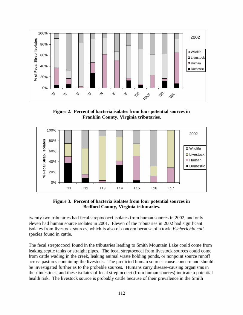
112

0%

20%

40%

60%

80%

100%

T0 T1 T2 T3 T4 T5 T6 T18

T19-2

0 T20

T21A

% o

f Fec

al S

trep

. Iso

late

s

Wildlife

Livestock

Human

Domestic

2002

Figure 2. Percent of bacteria isolates from four potential sources in Franklin County, Virginia tributaries.

0%

20%

40%

60%

80%

100%

T11 T12 T13 T14 T15 T16 T17

% F

ecal

Str

ep. I

sola

tes

Wildlife

Livestock

Human

Domestic

2002

Figure 3. Percent of bacteria isolates from four potential sources in Bedford County, Virginia tributaries.

twenty-two tributaries had fecal streptococci isolates from human sources in 2002, and only eleven had human source isolates in 2001. Eleven of the tributaries in 2002 had significant isolates from livestock sources, which is also of concern because of a toxic Escherichia coli species found in cattle. The fecal streptococci found in the tributaries leading to Smith Mountain Lake could come from leaking septic tanks or straight pipes. The fecal streptococci from livestock sources could come from cattle wading in the creek, leaking animal waste holding ponds, or nonpoint source runoff across pastures containing the livestock. The predicted human sources cause concern and should be investigated further as to the probable sources. Humans carry disease-causing organisms in their intestines, and these isolates of fecal streptococci (from human sources) indicate a potential health risk. The livestock source is probably cattle because of their prevalence in the Smith

113

Mountain Lake tributaries’ watersheds. Cattle are known to carry a toxic Escherichia coli species (0157:H7) in their intestines, which is another health risk to humans using the water as drinking water. The wildlife predictions are problematic since no solution is readily available; however, wildlife is not known to carry human pathogenic organisms or to pose a health risk. In 2003, the fecal coliform population determinations were made again on the tributaries, and the results are discussed above. In addition to the fecal coliform counts, the total coliform populations, E. coli counts, and gram-negative species identification were conducted on the tributary samples on Smith Mountain Lake in 2003. The total coliform counts were much higher than the fecal coliform counts, as would be expected in water samples. The percentage of E. coli bacteria found in the same samples varied between 1% and 60% of the total coliform populations. The new Virginia Department of Health standard per 100 mL water sample is 121 E. coli colonies. Our samples indicate that an exceedance of the standard using the old total coliform standard would result in the same number of exceedances as using the newer E. coli standard. In the BIOLOG method of determination of bacterial species identification, a similar result was found. Of the species identified on the fecal coliform plates, 27-65% were identified as E. coli. This finding is another indication that further study must be done comparing the different standards applied to water quality in reference to the bacterial contamination of Smith Mountain Lake and the human health risks and human influences on the lake water quality.

ACKNOWLEDGMENTS We would like to acknowledge the work of our lab coordinator Carol Love and the Ferrum College students (especially Tammy Manning, Eric Hoppis, Brian Owen, Curtis Bumgardner, Lindsay Cox, and Patricia Moyer) who assisted with this research in 2002 and 2003. Dr. Bob Pohlad assisted with the BIOLOG determinations, and Dr. Chuck Hagedorn and Amy Booth taught us all we know about the Antibiotic Resistance Assay.

REFERENCES American Public Health Association (APHA). 1995. Standard Methods for Examination of Water and Wastewater. 16th edition. Washington, D.C. Downie, N.M. and R.W. Heath. 1974. Basic Statistical Method. Harper and Row, Publishers. New York, N.Y. p. 314. Harwood, Valerie J., John Whitlock, and Victoria Withington. 2000. Classification of antibiotic resistance patterns of indicator bacteria by discriminate analysis: Use in predicting the source of fecal contamination in subtropical waters. Applied and Environmental Microbiology 66: 3698-3704.

114

PARTITIONING BETWEEN SEDIMENT-ATTACHED AND FREE FECAL INDICATOR BACTERIA

Leigh-Anne Henry and Theo A. Dillaha

Department of Biological Systems Engineering, Virginia Tech Blacksburg, VA 24061

lehenry@vt.edu

KEY WORDS: E. coli, TMDLs, bacteria, sediment, modeling

ABSTRACT

The development of TMDLs in accordance with section 303(d) of the 1972 Clean Water Act has heightened interest in the transport processes of fecal indicator bacteria. One major simplification in computer models used in TMDL design is to ignore bacteria attachment to sediment. Sediment-attached bacteria behave differently from nonattached bacteria, and may settle out of the water column faster, survive longer, or experience regrowth. Possible resuspension of bacteria from sediments poses a public health threat. This study will investigate different experimental methods available for differentiating between attached and free bacteria in a water sample and identify the best method for use in further research.

INTRODUCTION

There are numerous waterborne microorganisms that can cause human disease, including bacteria, protozoa, viruses, and helminthes. Because it would be difficult, expensive, and time-consuming to test waters designated for human use for the presence of all possible waterborne pathogens, waters are tested for only one or two organisms that are considered indicative of the presence of other common pathogens (Rosen 2001). Traditionally, fecal coliforms have been used as an indicator organism in monitoring biological water quality, but there has been a recent shift toward using E. coli, a specific type of fecal coliform, due to its higher correlation with many pathogens, including protozoa and viruses. Virginia will require monitoring of all freshwaters for E. coli by 2008. Water bodies with a geometric mean of E. coli counts higher than 126/100 mL or with a single sample count higher than 235/100 mL will be considered impaired for human use (VASWCB 2003).

Section 303(d) of the 1972 Clean Water Act mandates the development of Total Maximum Daily Loads (TMDLs) for water bodies that do not meet water quality standards in order to protect public and environmental health. A TMDL is a plan that identifies the maximum amount of pollutants that can enter a water body while still meeting water quality standards for its designated uses. The Virginia Department of Environmental Quality has identified 4,318 miles of streams that do not meet water quality standards and require TMDL development; of these, over 3,000 miles are impaired due to high levels of fecal coliform bacteria (VADEQ 2002). Nationally, pathogen indicators are the second most common pollutant responsible for identified water body impairments, accounting for 13% of the total number of listed water bodies (USEPA 1998).

115

In order to design TMDLs, sources of pollutants must be identified and decreased to levels that will keep the water body in compliance with water quality standards. The primary tools used to allocate discharge reductions to different sources are hydrologic computer simulation models. Because there has been relatively little monitoring of bacteria and there can be great variability in bacteria behavior, these models greatly simplify the process of bacteria transport. While this makes the simulation of bacteria transport possible even when little information is available, the predicted bacteria concentrations are less accurate. A greater understanding of the means by which bacteria are transported in a stream and their ultimate deposition or die-off would improve the understanding of the relationship between different possible sources of contamination and the current unacceptable levels of bacteria concentration.

Bacteria attachment to sediment can have a strong effect on the fate and transport of the bacteria but has been ignored in modeling due to a lack of data and information. The HSPF model, which is accepted and supported by the USDA for TMDL development, models bacteria as a dissolved pollutant. However, considerable evidence exists indicating that bacteria preferentially attach to sediment particles. Numerous studies of sediments underlying surface waters have found bacterial concentrations significantly higher than in the overlying waters. Higher sediment concentrations of bacteria have been documented in both freshwater (Matson et al. 1978, Stephenson and Rychert 1982, Irvine and Pettibone 1993) and marine waters (Erkenbrecker 1981, Ferguson et al. 1996), indicating that bacteria may be deposited with sediments, where they can accumulate over time.

Sediment-attached bacteria behave differently and exhibit different characteristics from free bacteria. Attachment to sediment particles decreases the settling time of these bacteria and influences their final deposition (Schillinger and Gannon 1985). There is also evidence that attachment or association with sediments may decrease bacteria die-off (Sherer et al. 1992, Howell et al. 1996) or stimulate regrowth (Desmarais et al. 2002) due to increased nutrient availability and/or protection from predators (Roper and Marshall 1978). Accumulation and maintenance of viable bacteria populations in stream sediments can pose a public health threat if these sediments are later disturbed, resuspending bacteria in the overlying waters. The “reappearance” of bacteria from stream sediments long after any contamination event has been induced by dredging (Grimes 1975), the passage of ships (Pettibone et al. 1996), cow crossings (Sherer et al. 1988), and artificial storm surges (McDonald et al. 1982). Because current hydrologic models do not account for bacteria attachment, sedimentation, regrowth, or resuspension, it is impossible to predict the time or magnitude of these events.

Determining the relative amounts of bacteria that exist as free cells or sediment-attached aggregates would allow modelers to better represent the process of bacteria transport. While there have been attempts to quantify the attachment of indicator bacteria to sediments using different experimental methods, no standard method for separating attached bacteria from free bacteria in a water sample is currently accepted.

116

EXPERIMENTAL METHODS

This study will be conducted during the summer of 2003. Two different methods of partitioning between sediment-attached and free bacteria will be tested to determine the most appropriate method for further research.

Bacterial behavior can vary widely between species and is very dependent on environmental conditions. To eliminate this variability, a pure culture of E. coli will be used, since it is the current indicator organisms accepted by Virginia for water quality monitoring. Samples of buffered dilution water will be inoculated with E. coli and sterilized sediment of different texture classes and mixed thoroughly to promote attachment. Each sample will be split into two equal subsamples. One subsample will be filtered using an 8 µm filter. The filtrate will be analyzed for E. coli concentration using the membrane filtration technique with mTEC agar (USEPA 2000). Those bacteria that pass through the 8 µm filter will be considered unattached, or free. The second subsample will be treated using a dispersion technique. The dispersion technique will break attachment to sediments and aggregation so that the sample can be analyzed for total bacteria concentration. Two different dispersion techniques will be tested: chemical dispersion using a surfactant, and ultrasonic dispersion using an ultrasonic cleaning bath. The difference in number between the total concentration and the free concentration will be considered the number of attached bacteria.

REFERENCES Desmarais, T.R., H.M. Solo-Gabriele, C.J. Palmer. 2002. Influence of soil on fecal indicator organisms in a tidally influenced subtropical environment. Applied and Environmental Microbiology 68(3): 1165-1172. Erkenbrecher, C.W. 1981. Sediment bacteria indicators in an urban shellfishing subestuary of the lower Chesapeake Bay. Applied and Environmental Microbiology 42(3): 484-492. Ferguson, C.M., B.G. Coote, N.J. Ashbolt, and I.M. Stevenson. 1996. Relationships between indicators, pathogens, and water quality in an estuarine system. Water Research 30(9): 2045-2054. Grimes, D.J. 1975. Release of sediment-bound fecal coliforms by dredging. Applied Microbiology 29: 109-111. Howell, J.M., M.S. Coyne, and P.L. Cornelius. 1996. Effect of sediment particle size and temperature on fecal bacteria mortality rates and the fecal coliform/fecal streptococci ratio. Journal of Environmental Quality 25(6): 1216-1220. Irvine, K.N. and G.W. Pettibone. 1993. Dynamics of indicator bacteria populations in sediment and river water near a combined sewer outfall. Environmental Technology 14: 531-542. Matson, E.A., S.G. Hornor, and J.D. Buck. 1978. Pollution indicators and other microorganisms in river sediment. Journal of the Water Pollution Control, Federation Jan.: 13-19.

117

McDonald, A., D. Kay, and A. Jenkins. 1982. Generation of fecal and total coliform surges by stream flow manipulation in the absence of normal hydrometeorological stimuli. Applied and Environmental Microbiology 44(2): 292-300. Pettibone, G.W., K.N. Irvine, and K.M. Monahan. 1996. Impact of a ship passage on bacteria levels and suspended sediment characteristics in the Buffalo River, New York. Water Research 30(10): 2517-2521. Roper, M.M. and K.C. Marshall. 1978. Effects of a clay mineral on microbial predation and parasitism of Escherichia coli. Microbial Ecology 4: 279-289. Rosen, B.H. 2001. Waterborne Pathogens in Agricultural Watersheds. NRAES-147. United States Department of Agriculture and Natural Resources Conservation Service Watershed Science Institute. Ithaca, N.Y. Schillinger, J.E., and J.J. Gannon. 1985. Bacterial adsorption and suspended particles in urban stormwater. Journal of the Water Pollution Control Federation 57(5): 384-389. Sherer, B.M., J.R. Miner, J.A. Moore, and J.C. Buckhouse. 1992. Indicator bacterial survival in stream sediments. Journal of Environmental Quality 21(4): 591-595. Sherer, B.M., J.R. Miner, J.A. Moore, and J.C. Buckhouse. 1988. Resuspending organisms from a rangeland stream bottom. Transactions of the ASAE 31(4): 1217-1222. Stephenson, G. R. and R. C. Rychert. 1982. Bottom sediment: a reservoir of Escherichia coli in rangeland streams. Journal of Range Management 35(1): 119-123. United States Environmental Protection Agency (USEPA). 1998. National Section 303(d) List Fact Sheet. http://oaspub.epa.gov/waters/national_rept.control (May 28, 2003). United States Environmental Protection Agency (USEPA). 2000. Improved enumeration methods for the recreational water quality indicators: Enterococcus and Escherichia coli. EPA/821/R-97/004. Virginia Department of Environmental Quality (VADEQ). 2002. Annual TMDL Report. http://www.deq.state.va.us/water/303d.html (May 28, 2003). Virginia Soil and Water Control Board (VASWCB). 2003. Water Quality Standards Homepage. http://www.deq.state.va.us/wqs/homepage.html (May 28, 2003).

118

SPECTROFLUOROMETRIC FILTER CHAMBER ASSAY TO IDENTIFY AND QUANTIFY E. COLI

Jean Nelson

US Army ERDC Topographic Engineering Center Alexandria, VA 22315

Jean.D.Nelson@erdc.usace.army.mil

Stanley Webb Department of Biology, Virginia Commonwealth University

Richmond, VA 23284

John Anderson US Army ERDC Topographic Engineering Center

Alexandria, VA 22315

KEY WORDS: E. coli, fluorescence, ec-mug, freshwater, indicator

ABSTRACT

The goal of this project was to develop a rapid assay for the detection and quantification of E. coli that was specific, sensitive, and comparable to standard methods. This project utilized the defined substrate 4-methylumbelliferyl-β-D-glucuronide (MUG), the selective EC medium, and spectrofluorometry. This new procedure generated same day results for detecting and quantifying E. coli in surface water. Fluorescence intensity was proportional to both incubation times and E. coli numbers, with ranges of 30 minutes to 11 hours and 108 cells to 1 cell (r2 = 0.988).

INTRODUCTION Surface waters are routinely analyzed for fecal coliforms, like E. coli, to assess microbiological quality. Some key challenges associated with us ing conventional culture methods in assessing water quality have been the need for 1) an improvement in specificity, 2) a reduction of assay time, and 3) a less labor intensive method (Sartory and Watkins 1999). These challenges ultimately led to the use of defined substrates for the detection of specific enzymes. E. coli possess the enzyme β-glucuronidase (GUD), which acts as a strong distinguishing characteristic for this organism (Shadix and Rice 1991). The fluorogenic substrate 4-methylumbelliferyl-β-D-glucuronide (MUG) can be used to demonstrate the activity of the GUD enzyme. This enzyme catalyzes the breakdown of MUG, cleaving 4-methylumbelliferone (4-MU), a coumarine derivative, and releasing the sugar portion of the MUG compound metabolized by the bacteria (Manafi 1998). Once the 4-MU is liberated, the MUG is considered “converted” and the fluorescence of 4-MU can be detected under long-wavelength UV light (Park et al. 1995). According to Standard Methods, the presence of such fluorescence ind icates a positive test for E. coli (APHA et al. 2000). EC-MUG medium is

119

accepted by EPA for detecting E. coli in water, and has been used for its ease of interpretation of target colonies and its ability to inhibit non-target organisms (Gaudet et al. 1996).

METHODS

This project focused on detecting and enumerating E. coli. The methods involved a selective medium, a selective temperature, and standard membrane filtration techniques for determining cell numbers (EPA 2000). EC-MUG (Difco) and an incubation temperature of 41.5°C were used. The standard membrane filtration techniques were performed concurrently with the new filter chamber assay throughout the project for direct comparison. Samples of both lab-spiked and river water were assessed. The E. coli used for all lab-spiked water samples was a recent isolate from the James River (Richmond, VA) that was grown as a shaker culture until the cells reached mid- log phase growth. Serial dilutions were made to achieve cell numbers ranging from 108 cells to 1 cell. Samples of river water were eventually analyzed to assess the specificity of the new assay.

The goal of the new assay was to minimize the initial cell numbers needed in a water sample, as well as the time periods needed for incubation, in order to detect and quantify E. coli. Sterivex (Millipore) are sterile, syringe-driven filtration devices (0.45 µm pore size; 2 mL void volume; 1000 mL maximum filtering capacity). Sterile syringes were used to push the desired volume of a water sample through the Sterivex to trap and concentrate the cells within the filter chamber. Syringes were then used to push EC-MUG into the Sterivex to trap approximately 2 mL of the medium inside. The ends of the Sterivex were sealed, and the Sterivex were then placed in a 41.5°C incubator. Incubation times ranged from 30 minutes to 11 hours. At intervals, the Sterivex were removed from the incubator, and the contents were collected in sterile tubes. The empty Sterivex devises were then discarded, still containing the bacterial cells. The collected filtrates consisted of EC-MUG and microbial metabolites that included the converted 4-MU fluorochrome. The sensitive “Fluorolog-3” spectrofluorometer (Jobin Yvon Horiba) was utilized to detect and measure the presence of the liberated 4-MU fluorochrome that exists once the E. coli have converted the MUG substrate. Sodium hydroxide was added to the 2 mL Sterivex filtrate samples to raise their pH to 10. The literature repeatedly stated that the fluorescence yielded by the converted MUG substrate was pH dependent and specifically that pH 10 was optimum for detecting this fluorescence (Hartman 1989, Davies and Apte 1996, Manafi 1998). Samples were then transferred to quartz cuvetes (1cm2) and subjected to spectrofluorometric analysis. Total Luminescence Spectroscopy (TLS) was applied to determine the optimum excitation and emission wavelength pairs for measuring the converted 4-MU fluorophore. TLS has been described as the simultaneous measurement of excitation, emission, and intensity spectra for a sample of interest (Lakowicz 1999, Sharma and Schulman 1999) and allows for the recording of a spectral signature that exists in three dimensions (Anderson et al. 2001). Also, Single Emission Spectroscopy or Excitation Scans were used to compare the resulting fluorescence intensities of the filtrate samples. The Excitation Scans involved collecting only two-dimensional data, which included excitation and fluorescence intensity values.

120

RESULTS

The spectral qualities of unconverted and converted EC-MUG were determined using TLS. Figure 1 shows the TLS contour plot for the converted EC-MUG filtrate. By altering the pH of converted EC-MUG filtrates to 10, they shared the same optimum excitation and emission wavelength pairs (Ex 365, Em 450 nm) as the control EC-MUG. However, the fluorescence intensity of the converted samples was greatly increased, generating a sharper, more defined peak. Finally, the increase in fluorescence intensity at pH 10 allowed for a more rapid detection of a positive response based on the release of 4-MU from MUG.

Figure 1. Total Luminescence Spectrum (TLS) for the converted EC-MUG

filtrate at pH 10 shown as a contour plot. Both variables (initial cell density and incubation time) played a key role in increasing the fluorescence intensity read by the spectrofluorometer. The relationship between initial cell numbers and resulting fluorescence due to different amounts of 4-MU being liberated was evident. Figure 2 shows the Single Emission Spectrum (Em 450 nm) of Sterivex filtrate samples using a 10-hour incubation period and 2000 to 100 cells. As incubation times were increased, resulting fluorescence increased. Also, when initial cell numbers were greater, the resulting fluorescence was greater.

DISCUSSION

A prediction model was generated relating incubation times and initial cell numbers to detect substrate conversion. The initial cell number- incubation time combinations that resulted in a fluorescence intensity value just above the control’s statistical upper limit were identified. The model answered the question: Given the incubation time, what cell numbers had to be present in the filtered water sample to give a positive response for conversion? Incubation times ranged from 30 minutes to 11 hours, while cell numbers ranged from 108 cells to 1 cell. It was clear by the model that the more cells present in the water sample, the less time would be required to detect the activity of those E. coli cells (r2=0.988). For example, only a 3-hour incubation period or less would be required to detect cell numbers in the millions per volume of water filtered. A 3- to 8-hour incubation period would be required to detect cell numbers in the

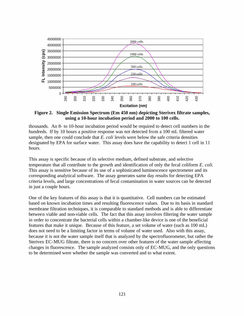
121

Figure 2. Single Emission Spectrum (Em 450 nm) depicting Sterivex filtrate samples, using a 10-hour incubation period and 2000 to 100 cells.

thousands. An 8- to 10-hour incubation period would be required to detect cell numbers in the hundreds. If by 10 hours a positive response was not detected from a 100 mL filtered water sample, then one could conclude that E. coli levels were below the safe criteria densities designated by EPA for surface water. This assay does have the capability to detect 1 cell in 11 hours. This assay is specific because of its selective medium, defined substrate, and selective temperature that all contribute to the growth and identification of only the fecal coliform E. coli. This assay is sensitive because of its use of a sophisticated luminescence spectrometer and its corresponding analytical software. The assay generates same day results for detecting EPA criteria levels, and large concentrations of fecal contamination in water sources can be detected in just a couple hours. One of the key features of this assay is that it is quantitative. Cell numbers can be estimated based on known incubation times and resulting fluorescence values. Due to its basis in standard membrane filtration techniques, it is comparable to standard methods and is able to differentiate between viable and non-viable cells. The fact that this assay involves filtering the water sample in order to concentrate the bacterial cells within a chamber-like device is one of the beneficial features that make it unique. Because of this feature, a set volume of water (such as 100 mL) does not need to be a limiting factor in terms of volume of water used. Also with this assay, because it is not the water sample itself that is analyzed by the spectrofluorometer, but rather the Sterivex EC-MUG filtrate, there is no concern over other features of the water sample affecting changes in fluorescence. The sample analyzed consists only of EC-MUG, and the only questions to be determined were whether the sample was converted and to what extent.

0

5000000

10000000

15000000

20000000

25000000

30000000

35000000

40000000

45000000

290

300

310

320

330

340

350

360

370

380

390

400

410

420

430

Excitation (nm)

FL In

tens

ity

(cps

)2000 cells

1000 cells

500 cells

250 cells

100 cells

122

ACKNOWLEDGMENTS

This project was supported in part by grants from the City of Richmond, Virginia, from the Defense Advanced Research Projects Agency (DARPA), and from Virginia Commonwealth University.

REFERENCES

Anderson, J.E., S.R. Webb, R.L. Fischer, K.M. Kester, and B.L. Brown. 2001. Baseline and in vivo total photoluminescence of endospore material using the parasitoid wasp C. congregata. Applied Spectroscopy 55: 684-689. APHA (American Public Health Association), AWWA (American Water Works Association), and WEF (Water Environment Federation). 2000. Standard Methods for the Examination of Water and Wastewater. Twentieth Edition. Davies, C.M. and S.C. Apte. 1996. Rapid enzymatic detection of fecal pollution. Water Science Technology 34: 169-171. EPA (U.S. Environmental Protection Agency). 2000. Membrane filter method for the simultaneous detection of total coliforms and Escherichia coli in drinking water. EPA 600-R-00-013. Office of Research and Development, U.S. Environmental Protection Agency. Cincinnati, Ohio. Gaudet, I.D., L.Z. Florence, and R.N. Coleman. 1996. Evaluation of test media for routine monitoring of Escherichia coli in nonpotable waters. Applied and Environmental Microbiology 62: 4032-4035. Hartman, P.A. 1989. The MUG (glucuronidase) test for Escherichia coli in food and water. In: Rapid Methods and Automation in Microbiology and Immunology. A. Balows, R.C. Tilton and A. Turano (Editors). Brixia Academic Press. Brescia, Italy. pp. 290-308. Lakowicz, J. 1999. Principles of Fluorescence Spectroscopy. Second Edition. Kluwer Academic Publishers. New York, N.Y. Manafi, M. 1998. New approaches for the fast detection of indicators, in particular enzyme detection methods (EDM). OECD Workshop Molecular Methods for Safe Drinking Water. Vienna, Austria. Park, S., E. Lee, D. Lee, S. Lee, and S. Kim. 1995. Spectrofluorometric assay for rapid detection of total and fecal coliforms from surface water. Applied and Environmental Microbiology 61: 2027-2029. Sartory, D.P. and J. Watkins. 1999. Conventional culture for water quality assessment: is there a future? Journal of Applied Microbiology Symposium Supplement 85: 225S-233S.

123

Shadix, L.C. and E.W. Rice. 1991. Evaluation of β-glucuronidase assay for the detection of Escherichia coli from environmental waters. Canadian Journal of Microbiology 37: 908-911. Sharma, A. and S. Schulman. 1999. Introduction to Fluorescence Spectroscopy. John Wiley and Sons. New York, N.Y.

124

MEETING FUTURE WATER SUPPLY NEEDS THROUGH THE DEVELOPMENT OF HIGH-YIELD GROUNDWATER WELLS, CITY OF ROANOKE, VIRGINIA

Brent Waters

Golder Associates Inc. 3701 Saunders Avenue, Richmond, VA 23227

Mike McEvoy

City of Roanoke 2012 South Jefferson Street, Roanoke, VA 24014

KEY WORDS: water supply, groundwater wells, electrical resistivity imagining

ABSTRACT Roanoke faced severe water shortages in the summers of 1999 and again in 2002, due in a large part to four consecutive years (1998 through 2002) of below normal precipitation. The city’s main water source, Carvin’s Cove Reservoir, is fed from three small streams with limited watershed catchment areas and highly variable stream discharge. In June 2002, the City of Roanoke acted preemptively and implemented a strict water conservation plan that included restrictions of non-essential water use such as lawn watering and car washing. In addition, Roanoke implemented a program to develop additional supplemental water supplies from deep underground aquifers beneath Roanoke. The groundwater wells will be used during periods of drought, peak water demand and/or low reservoir levels, and will be used to reduce the amount of water purchased from other jurisdictions, eliminate water use restrictions on the public, and to delay potential costly expansions of the existing water system infrastructure. Earlier efforts in 1999 focused on developing high capacity well(s) that are both easily accessible and did not require treatment. The project resulted in the successful developed three production wells that do not require treatment. Two wells were completed, tested, and permitted near Roanoke’s Carvins Cove water treatment plant and initially produced over 225 gallons per minute (gpm) each. A third well was located in southeastern Roanoke City. This well was drilled in carbonate formations near the Roanoke River. The well produces over 700 gpm and does not require treatment for turbidity or bacteria. The well does not even require disinfection according to Virginia Department of Health guidelines and the results of the extensive water quality testing. In 2002, the City of Roanoke decided to develop up to 6 million gallons per day (MGD) of additional groundwater supplies. This work started with the development of two highly productive wells with a combined yield of 2 MGD near the new Crystal Springs (microfiltration) water treatment plant. Up to an additional 4 MGD was developed from several high-yielding wells located in the Garden City and Riverdale area of the city. The new wells will eventually be tied into the city’s water distribution system and will greatly help meet peak summer water demand during the next drought and will help the region meet its projected water supply needs well into the future.

125

The new high-yield wells were located using traditional methods of geologic mapping and remote sensing analysis combined with sophisticated state-of-the-art electrical resistivity imaging techniques. The success in locating and developing so many high-yield wells in the Roanoke Valley region reflect major breakthroughs in our understanding of groundwater flow in fractured rock aquifers, and our ability to remotely identify and non- intrusively map the primary fracture pathways deep in the subsurface before a drill rig is brought to the site.

126

ENVIRONMENTAL RISK AND WELL-TO-HOME LOSS OF WATERBORNE RADON IN NORTHERN VIRGINIA COUNTIES

Fiorella V. Simoni, Douglas G. Mose, and George W. Mushrush

Department of Chemistry, George Mason University Fairfax, VA 22030 Dje42@aol.com

KEY WORDS: radon, well water, MCL

ABSTRACT At the present time, the United States Environmental Protection Agency’s (USEPA) proposed Maximum Contaminant Level (MCL) of 300 pCi/L for waterborne radon is for suppliers of municipal water systems. However, in our study measurements of waterborne radon in potable water from northern Virginia water wells, all exceed the proposed MCL. Water from wells in granite average about 3150 pCi/L, in schist about 1500 pCi/L, in sandstone about 1800 pCi/L, and in quartzite about 1250 pCi/L. In transport between municipal well storage tanks and homes, the waterborne radon typically drops only by about 20-40%. In our study, water consumed by homeowners still greatly exceeded the United States Environmental Protection Agency, USEPA’s MCL.

INTRODUCTION Uranium and the radioactive decay products of uranium such as Rn-222 are present in all rocks and soils. Because Rn-222 easily escapes from water, potable water from surface sources (e.g., rivers and lakes) contains almost no Rn-222. However, most groundwater contains Rn-222, often in excess of the 300 pCi/L MCL that has been proposed by the USEPA. The average Rn-222 in United States groundwater used as potable water is about 200-600 pCi/l. At this time, the waterborne radon limits in the Safe Drinking Water Act and its amendments apply only to municipal or multiple house systems (CFR 1996, Kocher 2001). The following paper reports on the radon concentrations in many homes and municipal water wells in northern Virginia. It will be seen that on average, most water wells supply potable water that exceeds the USEPA’s proposed MCL.

METHODS As part of our ongoing studies of indoor, soil and well water radon in Virginia homes, measurements were made of potable water radon in almost 1000 homes in Fairfax County. The water collections were made using the kitchen water faucet, after running the water at maximum flow for a few minutes until it seemed not to get any colder. Then the water faucet was turned to a slow non-turbulent flow. This was done to simulate the method most home occupants would use to obtain a glass of cold water.

127

When this study in Fairfax County (Mose et al. 1990) was almost completed, it became apparent that potable water from reservoirs had essentially no radon (all measurements were less than 100 pCi/L), and that many homes receiving well water had waterborne radon which greatly exceeded the USEPA’s MCL, Table 1. A subsequent study was made of high-productivity municipal wells in Prince William County, which is adjacent to and immediately south of Fairfax County.

Table 1. Waterborne radon and the geological units in which the water wells were drilled in Fairfax County.

Geological Number of Approximate Approximate Unit Wells Average Radon Median Radon

Granite 21 wells 3290 pCi/L 2910 pCi/L Schist 111 wells 2540 pCi/L 2380 pCi/L Sandstone 20 wells 1790 pCi/L 1540 pCi/L Quartzite 4 wells 1020 pCi/L 860 pCi/L

RESULTS AND DISCUSSION Granite is the most radioactive of all the common rock types. Granite in Prince William County produces the most radon-enriched water, Table 2. Wells in the granite in Prince William County have an average waterborne radon concentration of about 3150 pCi/L (median approximately 3200 pCi/L), more than ten times the USEPA’s proposed MCL.

Table 2. Waterborne radon and the geological unit in which the water wells were drilled in Prince William County.

Geological Number of Approximate Approximate Unit Wells Average Radon Median Radon

Granite 7 wells 3150 pCi/L 3200 pCi/L Schist 5 wells 1500 pCi/L 1700 pCi/L Sandstone 18 wells 1800 pCi/L 1600 pCi/L Quartzite 9 wells 1250 pCi/L 1000 pCi/L

In the study area, schist surrounds most of the granite. Elevated radon in groundwater from schist can occur because as uranium enriched granite melts move to higher crustal levels, some of their radioactive component can escape into hydrothermal fluids that leave cooling chambers of granite and enter the surrounding schist. In rocks such as granite and schist, much of the uranium is still on grain boundaries. As the uranium decays, radon forming on grain boundaries can easily accumulate in groundwater that passes through the rock. In this fashion, water wells in granite and schist tend to contain more waterborne radon than wells in the other rocks of Prince William County, Table 2. Wells in the schist have an average waterborne radon concentration of about 1500 pCi/L (median about 1700 pCi/L); about five times the USEPA’s proposed MCL.

128

In some areas of Virginia, red terrestrial sandstone locally has very high radioactivity because of hydrothermal enrichment along fractures. Hot water, moving in and out of these deep fractures, brought uranium from underlying granite into the sandstone, but only along the fault zones. A water well drilled in or near these fault zones can have high- levels of uranium, radium, and radon. The water wells drilled into sandstone that were sampled in this study (Table 2) have an average waterborne radon concentration of about 1800 pCi/L (median about 1600 pCi/L). Water wells in white quartzite have the lowest waterborne radon, probably because the quartzite formed from relatively clean beach sand having low uranium concentrations. The average waterborne radon concentration is about 1250 pCi/L (median about 1000 pCi/L), though the lowest is still more than four times the USEPA’s proposed MCL, Table 2. Almost all the well water systems had higher waterborne radon measurements at the water well than at the distribution sites. Typically the waterborne radon concentration dropped by about 20-40 percent. The radon decrease is probably due to loss by radioactive decay in the water pipes between the wells and the homes. In summary, many residents of Fairfax County and Prince William County in northeast Virginia use potable water from the county government, and most of the water originates from water wells. The USEPA’s proposed MCL for potable water is 300 pCi/L, but ground water from these water wells usually greatly exceeds this concentration. There is loss of radioactivity in the water lines between the wells and the homes and businesses, but the loss is only about 20-40 percent. At the present time, the USEPA has simply requested those operators of municipal and multiple house systems measure the waterborne level in their systems, and develop a plan for reducing the waterborne radon concentration if it exceeds 300 pCi/L. Consequently, the impact of the proposed MCL for waterborne radon has not been felt by the real estate industry, as has the USEPA’s recommended MCL of 4 pCi/L for airborne radon.

REFERENCES Code of Federal Regulations (CFR). 1996. Safe Drinking Act, Amendments: Federal Register 1412(b)(13), Section 109b. Kocher, D.C. 2001. Drinking water standards for radionuclides: The dilemma and a possible solution. Health Physics 80: 486-490. Mose, D.G., G.W. Mushrush, and C. Chrosniak. 1990. Radioactive hazard of potable water in Virginia and Maryland. Bulletin of Environmental Contamination and Toxicology 44: 508.

129

ARSENIC RELEASE DUE TO DISSIMILATORY REDUCTION OF IRON OXIDES IN PETROLEUM-CONTAMINATED AQUIFERS

Jonathan Roller, Madeline Schreiber, and Christopher Tadanier

Department of Geological Sciences, Virginia Tech Blacksburg, VA 24061

roller.1@vt.edu

Mark Widdowson Department of Civil and Environmental Engineering, Virginia Tech

Blacksburg, VA 24061

Jeffrey Johnson Environmental Systems and Technology

3708 South Main Street, Suite D, Blacksburg, VA 24060

KEY WORDS: arsenic, Fe(III) reduction, petroleum contamination

ABSTRACT Elevated arsenic concentrations in groundwater are commonly attributed to reducing environments. Arsenic sorbs strongly to mineral surfaces such as Fe(III) oxides. Microorganisms can couple oxidation of organic matter with Fe(III) reduction, promoting arsenic release to solution. The goal of this research is to quantify background and microbially-mediated arsenic release rates due to Fe(III) reduction in petroleum-contaminated aquifers. These rates will be determined by conducting controlled experiments using arsenic-bearing Fe(III) oxides and Fe(III)-reducing microorganisms. Results will be used to develop a mathematical model for arsenic release in petroleum-contaminated aquifers, which ultimately will be linked with a numerical biodegradation and transport code.

INTRODUCTION Petroleum contamination of shallow aquifers is a serious environmental problem facing the United States today. The primary sources of this contamination are terrestrial oil spills and leaking underground storage tanks. The United States Environmental Protection Agency (USEPA) has estimated that approximately 300,000 sites in the U.S. are contaminated by leaking underground storage tanks (USEPA 1993). Benzene, toluene, ethylbenzene, and xylene (BTEX) are the petroleum components of greatest concern due to their toxicity and high solubility in water. However, BTEX compounds can be readily degraded by a variety of aerobic and anaerobic microorganisms. Due to the low solubility of oxygen and the rapid consumption of oxygen by aerobic microorganisms, petroleum-contaminated aquifers often become anaerobic. It is in these aquifers that anaerobic microorganisms can couple BTEX oxidation with the reduction of terminal electron acceptors such as nitrate, Fe(III), sulfate, and carbon dioxide. Due to the abundance of iron oxides in aquifers, Fe(III) is a very important terminal electron acceptor.

130

Several studies have documented BTEX degradation by Fe(III)-reducing microorganisms (e.g., Lovely 1997). As Fe(III) in aquifers is reduced to soluble Fe(II), sorbed metals and nutrients may also be released to solution. For example, arsenic, which has a strong sorption affinity for iron oxides (Pierce and Moore 1982), can be released to water during microbial reductive dissolution of iron oxides (Cummings et al. 1999, Zobrist et al. 2000). Thus, one "unintended consequence" of BTEX biodegradation in petroleum-contaminated aquifers is that arsenic sorbed to iron oxides may be released to groundwater (Figure 1).

Fe(III) Reduction / Arsenic Fe(III) Reduction / Arsenic ReleaseRelease

As

Iron Oxide(FeIII)

Geobacter metallireducens

BTEX

e-

Iron Oxide

FeII As

Figure 1. Conceptual model of As release during Fe(III)-

reduction coupled with BTEX oxidation. Increases in groundwater arsenic concentrations have been observed in several petroleum-contaminated aquifers. However, understanding the processes that control this arsenic release is still very limited. To date, only one paper that addresses the potential for arsenic release due to the biodegradation of petroleum hydrocarbons has been published (Klinchuch et al.1999). The overall goal of this research project is to quantitatively determine arsenic release rates due to microbially mediated BTEX oxidation coupled to the reduction of Fe(III) in petroleum-contaminated aquifers.

EXPERIMENTAL DESIGN The first stage of this project involves determining background arsenic release by processes other than microbial BTEX oxidation. Fe(III) oxides will be synthesized in the form of ferrihydrite; arsenic will then be sorbed on their surfaces. These synthetic Fe(III) oxides will be introduced to a series of staged batch reactors containing the Fe(III) respiring microorganism Geobacter metallireducens. The electron donor for this experiment will be soil humic acid, a form of natural organic matter. Because Geobacter metallireducens is an obligate anaerobe, these experiments will be conducted in an anaerobic chamber. The influence of arsenic re-sorption onto the Fe(III) oxides will be evaluated using a flow-through reactor consisting of an Fe(III) oxide and bacteria "sandwich" held between two semi- permeable membranes (Figure 2). These

131

membranes will allow released arsenic to freely flow through the fixed bed to minimize re-sorption, but will prevent bacteria from being flushed out. Samples will be collected at selected intervals using a fraction collector. The arsenic species will be separated using a solid phase extraction column (Le et al. 2001) and quantified using graphite furnace atomic adsorption spectroscopy. The results of these experiments will yield background arsenic release rates in pristine aquifers.

Arsenic release rates in the presence of petroleum contamination will also be determined experimentally. The experimental design will be essentially the same as for the background arsenic release measurement, except that toluene will be used as the electron donor instead of natural organic matter. Geobacter metallireducens has been shown to readily degrade toluene in Fe(III)-reducing environments (Lovely 2000). Because toluene is a volatile compound, special care must be taken with the experimental apparatus to ensure that the reactors are gas-tight. By analyzing arsenic concentrations in the effluent, arsenic release rates in petroleum-contaminated aquifers can be determined.

EXPECTED RESULTS

Experimental results will be used to evaluate the relative impacts of natural vs. anthropogenic organic sources on arsenic release. After the experimental data have been collected, Fe(II) and arsenic (As(III) and/or As(V)) release rates (r, mol/m2/sec) will be calculated using the following expression:

where m is the effluent concentration of arsenic or Fe(II) in mol/kg, rf is the flow rate through the reactor (kg/sec), massiron oxide is the ferrihydrite mass (g), and Asp is the specific surface area of the ferrihydrite (m2/g). Release rates will be normalized to the moles of carbon oxidized. Statistical differences between the background arsenic release rates and arsenic release rates due to microbially mediated toluene oxidation will be evaluated at the 95% level of confidence with the Analysis of Variance (ANOVA) test. The final phase of this project will be to develop a mathematical model for arsenic release due to the coupling of toluene oxidation and Fe(III) reduction. The model will contain equations for

feed tank

sample collection

fixed bed

Close-up of iron oxide and microbe “sandwich” in fixed bed

Figure 2. Design of flow-through reactor experiment.

([mS])(rf) (massiron oxide)(Asp)

r =

132

toluene oxidation, Fe(III) oxide reduction, arsenic release, and arsenic transport. This model will ultimately be linked with the biodegradation program SEAM3D (Waddill and Widdowson 1997). Application of the enhanced SEAM3D to field sites will allow for improved evaluation of the potential for arsenic release and subsequent transport in both pristine and petroleum-contaminated aquifers.

REFERENCES Cummings, D.E., F. Caccavo, et al. 1999. Arsenic mobilization by the dissimilatory Fe(III)-reducing bacterium Shewanella alga BrY. Environmental Science and Technology 33(5): 723-729. Klinchuch, L.A., T. Delfino, J. Jefferson, and J. Waldron. 1999. Does biodegradation of petroleum hydrocarbons affect the occurrence or mobility of dissolved arsenic in groundwater? Environmental Geosciences 6(1): 9-24. Le, X. C. and S. Yalcin. 2001. Speciation of arsenic using solid phase extraction cartridges. Journal of Environmental Monitoring 3(1): 81-85. Lovley, D. R. 1997. Potential for anaerobic bioremediation of BTEX in petroleum-contaminated aquifers. Journal of Industrial Microbiology and Biotechnology 18: 75-81. Lovely, D.R. 2000. Environmental Microbe-Metal Interactions. ASM Press Washington, D.C. Pierce, M. and C. Moore (1982). Adsorption of arsenite and arsenate on amorphous iron hydroxide. Water Resources 16: 1247-1253. USEPA. 1993. Cleaning Up the Nation's Waste Sites: Markets and Technology Trends. EPA 542-R-96-010. EPA Office of Solid Waste and Engineering Response. Washington, D.C. Waddill, D. and M. Widdowson 1997. SEAM3D: A Numerical Model for Three-Dimensional Solute Transport and Sequential Electron-Acceptor Based Bioremediation in Groundwater. Virginia Polytechnic Institute and State University. Blacksburg, Va. Zobrist, J., P.R. Dowdle, et al. 2000. Mobilization of arsenite by dissimilatory reduction of adsorbed arsenate. Environmental Science and Technology 34(22): 4747-4753.

133

STUDY OF A MODEL FOR THE PLANT UPTAKE OF ORGANIC CONTAMINANTS

Jason P. Barbour, James A. Smith, Jen L. Buckels, and Tim F. Wenk Department of Civil Engineering, University of Virginia Thornton Hall, Room B228, Charlottesville, VA 22903

jpb3h@virginia.edu

KEY WORDS: phytoremediation, lipid, ground water contamination

ABSTRACT The study of chemical uptake by plants is important as it relates to crop contamination and phytoremediation. Several relationships have been developed to describe the level of plant contamination. Recently, a relationship has been proposed that relies on knowledge of the composition of the plant and the partition coefficients of the solute. We hypothesize that the dominant factors affecting nonionic organic pollutant transport are the plant lipid content and the octanol-water partition coefficient of the solute. We have conducted lipid analyses on several grasses and alfalfa and have begun to quantify the rate of pollutant uptake by several plant types. Preliminary results show that plant lipid content can be highly variable between plants, and that pollutant uptake is indeed influenced by solute partition into lipid reservoirs.

INTRODUCTION Plant contamination has been widely studied since the advent of several organochlorine pesticides in the 1950s (Chiou et al. 2001). Although the accumulation of harmful chemicals in crops was the original focus, this field of study has now broadened to include the use of plants as a tool to remove contaminants from soil and groundwater— a process often referred to as phytoremediation. Researchers have identified numerous factors that affect the rate and amount of contaminant uptake. The soil type, particularly its organic-carbon content, is known to have a significant impact on the uptake of organic chemicals (Topp et al. 1986). The properties of the contaminant and the plant are known to be important as well. Studies have shown a correlation between root uptake and the octanol-water partition coefficient (Briggs et al. 1982, Topp et al. 1986). Thus, the contamination in the plant is thought to depend on the properties of the soil, contaminant, and plant; the contamination level in the soil; and the time of exposure (Chiou et al. 2001). Several studies have been conducted in a soil- free environment to simplify the study of contaminant transport (Briggs et al. 1982, McFarlane et al. 1987, Shone and Wood 1974). Shone and Wood (1974) defined the root concentration factor (RCF) as the ratio of the chemical’s concentration in roots to its concentration in the external water solution. Initial correlations developed between RCF and the octanol-water partition coefficient were limited to similar plants with non-woody roots (Briggs et al. 1982, Topp et al. 1986). The transpiration stream concentration factor (TSCF) is defined as the ratio of the solute concentration in the transpiration stream to its concentration in the external solution. The TSCF reaches a maximum equilibrium value of 1.0 for passive uptake (Shone and Wood 1974). Therefore, the TSCF can

134

be used as a measure of the approach to equilibrium. Because of the difficulty in directly measuring the concentration in the transpiration stream, the TSCF must be estimated based on other data, including plant transpiration rates. Briggs et al. (1982) have presented data showing that the TSCF values are at a maximum for solutes with log Kow in the range of 1 to 3. Another measure of the approach to equilibrium is based on the solute partition coefficients and the water, lipid, and carbohydrate fractions in the plant, and is defined below (Chiou et al. 2001): αpt = (Cpt / Cw) / (fpw + fch Kch + flip Klip) where αpt is the quasi-equilibrium factor; Cpt is the concentration of chemical in the plant (mg of chemical/kg of plant); Cw is the concentration of chemical in the external solution (mg of chemical/kg of water); fpw, fch, and flip are the mass fractions of water, carbohydrate, and lipids in the plant, respectively; Kch is the carbohydrate-water partition coefficient, and Klip is the lipid-water partition coefficient. The calculation of αpt demands knowledge of the plant makeup but provides a more complete description of the partitioning processes in the plants and requires only that the bulk plant concentration be measured. Chiou et al. (2001) have calculated αpt values for previously published data. Although their analyses required several assumptions, their results appear to be in agreement with the RCF data from Briggs et al. (1982). No attempt was made to validate the model with the TSCF data from this study, due to the short timeframe of the study and the lack of reported contamination data for the plant tissues. Given the relative absence of time-dependent pollutant uptake data by plants of known lipid content, our goal is to conduct experiments to more clearly elucidate the roles of the octanol-water partition coefficient of the solute and the lipid content of the plant in the uptake of nonionic solutes from water to plants. As a first step, we have quantified the lipid contents of several plants at different life stages and begun to measure the uptake of two nonionic solutes (trichloroethene (TCE) and 1,2-dichlorobenzene (DCB)) in these plants. We have designed our experiments to quantify the quasi-equilibrium factor (αpt) as a function of time to gain insight into both the equilibrium states achieved and the rate to equilibrium.

METHODS To provide plant composition data for use in calculating αpt values, the following procedure was devised, based on a similar procedure developed by Dr. David Orcutt at Virginia Tech. Plant samples are freeze-dried at the temperature of liquid nitrogen and then ground to a fine powder. A 2:1 chloroform/methanol solution is used to extract the lipids and carbohydrates from the remainder of the plant. The chloroform/methanol solution is evaporated under a nitrogen stream, leaving the carbohydrates and lipids behind. Chloroform is used to re-dissolve the lipids, which are removed to a new container where the chloroform is evaporated under a nitrogen stream. Lipid and carbohydrate masses are then determined gravimetrically. To obtain αpt values as a function of time, plants were grown in containers approximately 36 inches long and 1.5 inches wide and supported by 3 mm glass beads. The plants received nutrients from a flow-through water delivery system. Once the plants reached the desired level of maturity, a chemical contaminant was added to the flow-through water solution at a constant

135

Table 1: Lipid and water content data.

rate using a syringe pump. The water flow rate was chosen such that the chemical concentration in the water was approximately constant over the length of the bed. Each day, several of the plants were removed for analysis of the level of contamination. The plants were placed in a chloroform/methanol solution to extract the chemical. The chemical concentration in the resulting solution was analyzed with a gas chromatograph.

RESULTS AND DISCUSSION The United States Department of Agriculture has compiled a large database of plant composition information for edible plants. For inedible plants, very little data are available, but are considered vital to developing an understanding of the solute/plant interaction. The lipid- and water-content data for the plants are given in Table 1. The data show there is a wide range of lipid values, even for the relatively similar plants that were tested. Based on the data available, it appears that the lipid content increases with plant age. Preliminary data (not shown) also seems to indicate that, in general, the shoots of the plant have a higher lipid content than the roots.

Grass Age (weeks)

Water (wt%)

Lipid (wt%, wet basis)

Kentucky Fescue 1 91 0.44Kentucky Fescue 2 87 0.69Kentucky Fescue 4 86 1.42Annual Ryegrass 2 92 1.08Perennial Ryegrass 2 88 0.61Highland Bentgrass 3 93 0.51Highland Bentgrass 5 93 0.68Little Bluestem 2 85 0.53Alfalfa 2 92 0.53

By examining Chiou’s model, there are several inferences that can be made. First, lipophilic compounds (i.e., those with high log Kow values) will be stored in the plants in higher concentrations than hydrophilic compounds at equilibrium, assuming the same concentration of the chemical in the external solution. The assumption could also be made that passive transport αpt will approach unity as the system goes to equilibrium. Additionally, it is reasonable that it will take lipophilic compounds longer to reach equilibrium due to the greater amount of solute that must be translocated into the plant from the solution and retardation of lipophilic compounds by significant lipid-water partitioning. Thus far, several short-term experiments have been completed. These tests used TCE and DCB, which have log Kow values of 2.53 and 3.38, respectively. Figure 1 shows data from one set of experiments with alfalfa, for which the solute concentrations in the external water solution were 8 ppm. Chiou’s model predicts that the alpha values for all chemicals will continue to rise and eventually reach unity. Since the time to equilibrium will be a period of several weeks or months, the plant will grow significantly during the course of the experiment, diluting the solute

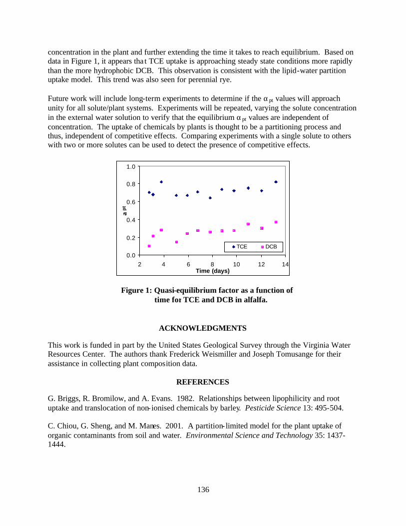
136

Figure 1: Quasi-equilibrium factor as a function of time for TCE and DCB in alfalfa.

concentration in the plant and further extending the time it takes to reach equilibrium. Based on data in Figure 1, it appears tha t TCE uptake is approaching steady state conditions more rapidly than the more hydrophobic DCB. This observation is consistent with the lipid-water partition uptake model. This trend was also seen for perennial rye. Future work will include long-term experiments to determine if the αpt values will approach unity for all solute/plant systems. Experiments will be repeated, varying the solute concentration in the external water solution to verify that the equilibrium αpt values are independent of concentration. The uptake of chemicals by plants is thought to be a partitioning process and thus, independent of competitive effects. Comparing experiments with a single solute to others with two or more solutes can be used to detect the presence of competitive effects.

0.0

0.2

0.4

0.6

0.8

1.0

2 4 6 8 10 12 14Time (days)

αp

t

TCE DCB

ACKNOWLEDGMENTS This work is funded in part by the United States Geological Survey through the Virginia Water Resources Center. The authors thank Frederick Weismiller and Joseph Tomusange for their assistance in collecting plant composition data.

REFERENCES G. Briggs, R. Bromilow, and A. Evans. 1982. Relationships between lipophilicity and root uptake and translocation of non- ionised chemicals by barley. Pesticide Science 13: 495-504. C. Chiou, G. Sheng, and M. Manes. 2001. A partition- limited model for the plant uptake of organic contaminants from soil and water. Environmental Science and Technology 35: 1437-1444.

137

C. McFarlane, T. Pfleeger, and J. Fletcher. 1987. Transpiration effect on the uptake and distribution of bromacil, nitrobenzene, and phenol in soybean plants. Journal of Environmental Quality 16: 372-376. M.G.T. Shone, and A.V. Wood. 1974. A comparison of the uptake and translocation of some organic herbicides and a systemic fungicide by barley. I. Adsorption in relation to physico-chemical properties. Journal of Experimental Botany 25: 390-400. E. Topp, I. Scheunert, A. Attar, and F. Korte. 1986. Factors affecting the uptake of C-14 labeled organic chemicals by plants from soil. Ecotoxicology and Environmental Safety 11: 219-228.

138

INVESTIGATION INTO HEAVY METAL UPTAKE BY WASTEWATER SLUDGE

Tomika Bethea, Khalila Porome, Zaron Johnson, Eric Hayes, and Isai T. Urasa Department of Chemistry, Hampton University

Hampton, VA 23668 isai.urasa@hamptonu.edu

KEY WORDS: metals, sludge, metal uptake

ABSTRACT

The distribution, mobility, and bioavailability of heavy metals in soils, surface water, and ground water are of major interest and concern from both environmental and geochemical standpoints. Wastewater sludge represents an important anthropogenic factor whose impact is not fully understood. In the past, incineration and land filling were common practices for discarding wastewater sludge. However, as local and state laws governing the disposal of these materials have become more stringent, land application has been used as an alternative for disposing of wastewater biosolids. While land application has the advantage of providing many of the nutrients required for plant growth, published studies have shown that its impact can vary widely and is influenced by a number of factors, including the source of the sludge; the organic matter content of the sludge; the form in which the sludge is applied; and the prevailing conditions of the receiving soils. Preliminary studies conducted in our laboratory with composted sludge have shown that this material has a high affinity for metals. This metal uptake property appears to be particularly pronounced for lead (Pb), for which the material showed a retention capacity of 15% of its weight. The metal uptake process is accompanied by the release of an equivalent amount of calcium. Based on the results of this preliminary work, it appears that metal uptake by composted biosolids involves phosphates. These phosphates may be associated with minerals, such as apatite, present in the sludge. The similarity between composted sludge and apatite with respect to their interaction with heavy metals not only suggests the presence of apatite or apatite-like material in the sludge, but also has two major implications. First, the apparently high affinity for metals can cause undesirable geochemical shifts of essential metals if this material is applied on agricultural land. This could lead to the immobilization of essential metals for plant growth, such as Cu, Fe, and Zn. Second, the apparently high preference of Pb could lead to the development of this material for use in recovering and recycling industrial heavy metals in waste streams, remediation, preconcentration of dilute solutions prior to analytical measurements, and in field sampling. The purpose of this study was to conduct an investigation of the behavior of biosolids towards heavy metals, verifying the metal-uptake process and identifying the attendant influential factors and possible mechanisms. This kind of information is necessary before attempts can be made to develop the material for possible practical applications as suggested above, or implementing measures to prevent adverse effects that may result from its use on agricultural soils.

139

DISSOLUTION, TRANSPORT, AND FATE OF LEAD SHOT AND BULLETS ON SHOOTING RANGES

Caleb Scheetz and J. Donald Rimstidt

Department of Geological Sciences, Virginia Tech 4044 Derring Hall, Blacksburg, VA 24061

cscheetz@vt.edu KEY WORDS: lead corrosion, hydrocerussite, shooting ranges, soils

ABSTRACT Lead contamination from shot and bullets on shooting ranges is receiving increasing scrutiny. Shooting ranges concentrate heavy metals especially lead, as spent shot and bullets. Hydrocerussite has been identified by X-ray diffraction as the predominate corrosion phase in the weathered coating removed from lead shot at the Blacksburg, Virginia shooting range. Hydrocerussite becomes increasingly soluble in acidic pH conditions. Acidic shooting range conditions, therefore, have the potential to mobilize lead into the soil horizon.

INTRODUCTION

Lead has been used extensively to manufacture shot and bullets throughout the history of firearms. Shooting ranges provide safe controlled environments for the discharge of firearms by recreational shooters, as well as police and military personnel. The congregation of shooters at shooting ranges concentrates spent lead shot and bullets onto very small parcels of land. The EPA estimates that roughly 1.6x108 lbs of lead shot and bullets enter the U.S. environment each year at roughly 9000 non-military outdoor shooting ranges (EPA 2001). Previous analyses have reported shot, on average, contain up to 97% metallic lead and bullets contain up to 90% metallic lead (Scheuhammer et al. 1995). Lead toxicity to humans and wildlife has been extensively documented over the past several decades. In humans, prolonged exposure to high concentrations of lead can lead to brain, nervous system, and reproductive damage (Nriagu 1978). Children are at particular risk because their bodies absorb lead more efficiently, thus even low concentrations of lead can be damaging to a child’s health (Nriagu 1978). The effects of lead poisoning in waterfowl by ingestion of lead shot are well documented by Feierabend (1983). Concerns have been raised about the environmental impact and ultimate fate of lead on shooting ranges. We have assessed the dissolution, transport, and fate of lead derived from shot at the U.S. Forest Service’s shotgun range located west of Blacksburg, Virginia off of Route 460 in the Jefferson National Forest. A previous study conducted at this range reported surface lead concentrations as high as 5,000 g Pb/m2 (Craig et al. 2002). This study also reported that since the shotgun range was opened in 1993 through 2000, 11.1 metric tons of lead shot have accumulated on site, with an average annual deposition rate of 1.4 metric tons of lead shot per year (Craig et al. 2002).

140

LEAD CORROSION, SOLUBILITY, AND TRANSPORT

Metallic lead is stable at low redox potentials and slightly acidic to extremely basic pH conditions. As metallic lead corrodes, it consumes both oxygen and hydrogen ions,

Pb(s) + 1/2O2 + 2H+ = Pb2+ + H2O;

thus the environment at the metal surface should have a low pe and high pH. The lead oxidation products hydrocerussite (Pb3(CO3)2(OH)2) and massicot (PbO), which coat and passivate the metal surface are stable at low pe and high pH as is illustrated in Figure 1.

Figure 1. Stability relationships of lead compounds in water at 25°C and 1 Atm.

[Pb] = 10-3 m, [CO3 total] = 10-4 m The solubility of hydrocerussite is strongly pH dependent with a minimum solubility near pH 9.0. Decreasing pH increases hydrocerussite’s solubility dramatically, so that it is about four orders of magnitude higher at pH 5.5 than it is at pH 9 (Figure 2). Acidification of soil by acid rain, decaying organic matter, or other means has the potential to dissolve hydrocerussite and mobilize the lead as an aqueous species.

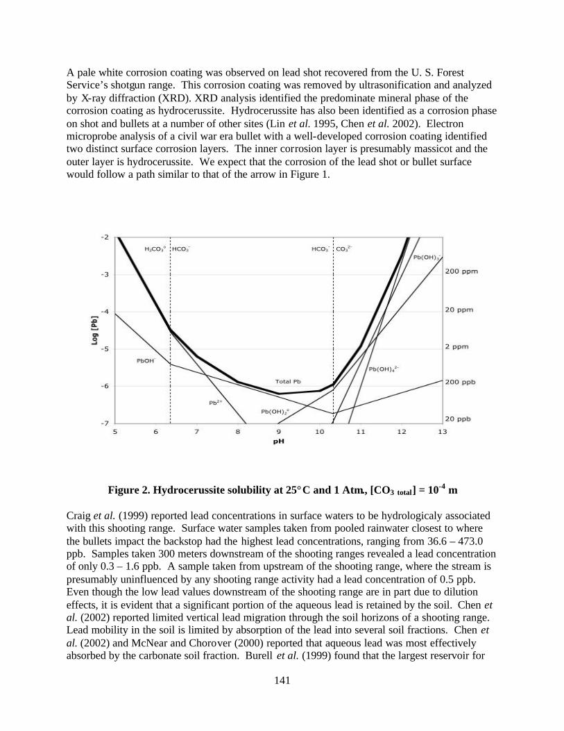
141

A pale white corrosion coating was observed on lead shot recovered from the U. S. Forest Service’s shotgun range. This corrosion coating was removed by ultrasonification and analyzed by X-ray diffraction (XRD). XRD analysis identified the predominate mineral phase of the corrosion coating as hydrocerussite. Hydrocerussite has also been identified as a corrosion phase on shot and bullets at a number of other sites (Lin et al. 1995, Chen et al. 2002). Electron microprobe analysis of a civil war era bullet with a well-developed corrosion coating identified two distinct surface corrosion layers. The inner corrosion layer is presumably massicot and the outer layer is hydrocerussite. We expect that the corrosion of the lead shot or bullet surface would follow a path similar to that of the arrow in Figure 1.

Figure 2. Hydrocerussite solubility at 25°C and 1 Atm., [CO3 total] = 10-4 m

Craig et al. (1999) reported lead concentrations in surface waters to be hydrologicaly associated with this shooting range. Surface water samples taken from pooled rainwater closest to where the bullets impact the backstop had the highest lead concentrations, ranging from 36.6 – 473.0 ppb. Samples taken 300 meters downstream of the shooting ranges revealed a lead concentration of only 0.3 – 1.6 ppb. A sample taken from upstream of the shooting range, where the stream is presumably uninfluenced by any shooting range activity had a lead concentration of 0.5 ppb. Even though the low lead values downstream of the shooting range are in part due to dilution effects, it is evident that a significant portion of the aqueous lead is retained by the soil. Chen et al. (2002) reported limited vertical lead migration through the soil horizons of a shooting range. Lead mobility in the soil is limited by absorption of the lead into several soil fractions. Chen et al. (2002) and McNear and Chorover (2000) reported that aqueous lead was most effectively absorbed by the carbonate soil fraction. Burell et al. (1999) found that the largest reservoir for

142

aqueous lead was the exchangeable or organic fraction. It is clear that site-specific soil chemistry has a significant role in lead mobility. Selective sequential chemical extractions (SSCE) were performed on the Blacksburg shooting range to quantify total lead concentration in five soil fractions: soil solution, exchangeable, bound to carbonates, bound to iron and manganese oxides, and bound to organic matter, as outlined in Tessier et al. (1979). Preliminary SSCE results indicate that carbonates, iron and manganese oxides, and organic matter are incorporating the majority of the aqueous lead in the surface soil horizon, thus limiting the mobility and bioavailability of the aqueous lead.

RECOMMENDATIONS Prior to the construction of a new shooting range, site selection should include, lead sorption capacity tests, pH evaluations, and SSCE’s on the prospective range soil to determine its lead absorption potential. Lime should be added to the range surface to raise the soil pH to near the minimum solubility of hydrocerussite at pH 9. A retention pond should be constructed immediately down gradient of the proposed range where topographically feasible, to prohibit off-range transport of physically eroded soil particles. Existing shooting ranges should frequently lime the range surface and construct a retention pond if possible.

REFERENCES

Bruell, R., N.P. Nikolaidis, and R.P. Long. 1999. Evaluation of remedial alternatives of lead from shooting range soil. Environmental Engineering Science16: 403-414.

Chen, M., S. Daroub, L. Ma, W. Harris, and X. Cao. 2002. Characterization of lead in soils of a rifle/pistol range in central Florida, USA. Soil and Sediment Contamination 11: 1-17. Craig, J.R., J.D. Rimstidt, C.A. Bonnaffon, T.K. Collins and P.F. Scanlon. 1999. Surface water transport of lead at a shooting Range. Bulletin of Environmental Contamination and Toxicology 63: 312-319. Craig, J.R., D. Edwards, J.D. Rimstidt, P.F. Scanlon, T.K. Collins, O. Schabenberger, and J.B. Brich. 2002. Lead distribution on a public shooting range. Environmental Geology 41: 873-882. Environmental Protection Agency (EPA). 2001. Best Management Practices for Lead at Outdoor Shooting Ranges. Feierabend, J.S. 1983. Steel shot and lead poisoning in waterfowl. In: National Wildlife Federation, Scientific and Technical Series 8. Lin, Z., B. Comet, U. Qvarfort, and R. Herbert. 1995. The chemical and mineralogical behavior of Pb in shooting range soils from central Sweden. Environmental Pollution 89: 303-309.

143

McNear, D.H. Jr. and J. Chorover. Speciation of lead in soils from bullets in firing ranges. In: Annual Meetings Abstract: 51. ASA/CSSA/SSSA, Minneapolis, Min. Nov. 5-9, 2000. Nriagu, J.O. 1978. The Biogeochemistry of Lead in the Environment Part A & B. Elsevier/North-Holland Biomedical Press. New York, N.Y. Scheuhammer, A.M., and S.L. Norris. 1995. A Review of the Environmental Impacts of Lead Shotshell Ammunition and Lead Fishing Weights in Canada. Rep. 88. Minister of Environment, Canadian Wildlife Services. Ottawa, Ontario. Tessier, A., P.G.C. Campbell, M. Bisson. 1979. Sequential extraction procedure for the speciation of particulate trace metals. Analytical Chemistry 51: 844-851.

144

SCREENING OF LEAD ION ADSORBENTS IN AQUEOUS MEDIA

Tarek Abdel-Fattah, Larry K. Isaacs, and Kelly B. Payne Department of Biology, Chemistry and Environmental Science; Christopher Newport University

Newport News, VA 23606 fattah@cnu.edu

KEY WORDS: adsorbents, lead, zeolites, activated carbon, molecular sieves, chabazite, clinoptilolite

INTRODUCTION The state of Virginia has at least 35 outdoor shooting ranges, not counting those that belong to the military. To comply with environmental regulations and protect the environment, lead (Pb) contaminates in soil and stormwater at small arms ranges (SAR) need to be immobilized. Although metallic Pb from unweathered bullets in soil has low chemical reactivity, it is possible to mobilize Pb in soil and aqueous media with low pH, significant changes in ionic strength, or changes in the reduction oxidation potential. Some of the mobilized Pb attach to soil organic matter (Pickering, 1986) or inorganic soil components through adsorption or ion exchange (Mellor and McCartney 1994). Total lead concentrations in wastewaters may exceed acceptable water quality effluent standards for discharge to waters of the United States. Zeolites have been studied as effective Pb2+ adsorbents (Abdel-Fattah and Payne 2001, Caro et al. 2000). Screening of various lead ion adsorbent materials via batch adsorption studies were investigated to determine their comparative performance and optimal operating conditions at various pH levels, competing ion strengths, and temperatures. Adsorbent materials such as activated carbon, naturally occurring zeolites (Clinoptilolite and Chabazite) and molecular sieves (13X and 5A) are point-of-use materials for mitigating wastewater. New technology organo-silicate nanocomposites (HMS, MCM-41 and MCM-48) also provide promising adsorbent results. The relative average lead adsorption was: 13X > Chabazite > Clinoptilolite > 5A > MCM-41 > HMS > MCM-48 >activated carbon.

MATERIALS AND METHODS

Zeolites are naturally occurring, porous, hydrated aluminosilicates with exchangeable cations such as sodium and potassium. Clinoptilolite and chabazite (volcanic in origin, mined in Arizona, and obtained from GSA Resources, Inc.) are being studied due to their availability at a very low cost. 13X (sodium potassium aluminosilicate) and 5A (sodium calcium aluminosilicate) are synthetic versions of naturally occurring zeolites with well-documented behavior (obtained from Aldrich). The activated carbon used in this study is randomly stacked microcrystallines of graphite produced from coal (obtained from Calgon Carbon Corporation). The use of firm or trade names does not constitute a recommendation or endorsement by the Virginia Water Resources Research Center.

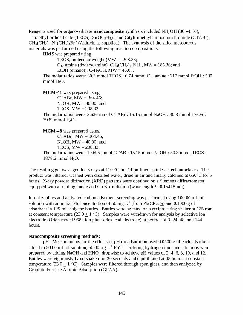
145

Reagents used for organo-silicate nanocomposite synthesis included NH4OH (30 wt. %); Tetraethyl-orthosilicate (TEOS), Si(OC2H5)4; and Cityltrimethylammonium bromide (CTABr), CH3(CH2)15N+(CH3)3Br - (Aldrich, as supplied). The synthesis of the silica mesoporous materials was performed using the following reaction compositions:

HMS was prepared using TEOS, molecular weight (MW) = 208.33; C12 amine (dodecylamine), CH3(CH2)11NH2, MW = 185.36; and EtOH (ethanol), C2H5OH, MW = 46.07.

The molar ratios were: 30.3 mmol TEOS : 6.74 mmol C12 amine : 217 mmol EtOH : 500 mmol H2O. MCM-41 was prepared using

CTABr, MW = 364.46; NaOH, MW = 40.00; and TEOS, MW = 208.33.

The molar ratios were: 3.636 mmol CTABr : 15.15 mmol NaOH : 30.3 mmol TEOS : 3939 mmol H2O. MCM-48 was prepared using

CTABr, MW = 364.46; NaOH, MW = 40.00; and TEOS, MW = 208.33.

The molar ratios were: 19.695 mmol CTAB : 15.15 mmol NaOH : 30.3 mmol TEOS : 1878.6 mmol H2O.

The resulting gel was aged for 3 days at 110 °C in Teflon- lined stainless steel autoclaves. The product was filtered, washed with distilled water, dried in air and finally calcined at 650°C for 6 hours. X-ray powder diffraction (XRD) patterns were obtained on a Siemens diffractometer equipped with a rotating anode and Cu-Kα radiation (wavelength λ=0.15418 nm). Initial zeolites and activated carbon adsorbent screening was performed using 100.00 mL of solution with an initial Pb concentration of 50 mg L-1 (from Pb(ClO 4)2) and 0.1000 g of adsorbent in 125 mL nalgene bottles. Bottles were agitated on a reciprocating shaker at 125 rpm at constant temperature (23.0 + 1 oC). Samples were withdrawn for analysis by selective ion electrode (Orion model 9682 ion plus series lead electrode) at periods of 3, 24, 48, and 144 hours. Nanocomposite screening methods:

pH. Measurements for the effects of pH on adsorption used 0.0500 g of each adsorbent added to 50.00 mL of solution, 50.00 µg L-1 Pb2+. Differing hydrogen ion concentrations were prepared by adding NaOH and HNO3 dropwise to achieve pH values of 2, 4, 6, 8, 10, and 12. Bottles were vigorously hand shaken for 30 seconds and equilibrated at 48 hours at constant temperature (23.0 + 1 oC). Samples were filtered through spun glass, and then analyzed by Graphite Furnace Atomic Adsorption (GFAA).

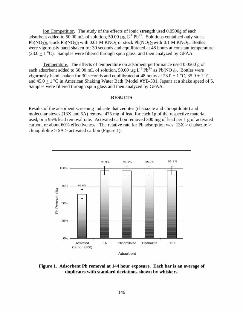
146

63.6%

96.9% 96.9% 96.3% 96.9%

0%

25%

50%

75%

100%

ActivatedCarbon (300)

5A Clinoptilolite Chabazite 13X

Adsorbent

Pb

Rem

oval

(%)

Ion Competition. The study of the effects of ionic strength used 0.0500g of each adsorbent added to 50.00 mL of solution, 50.00 µg L-1 Pb2+. Solutions contained only stock Pb(NO3)2, stock Pb(NO3)2 with 0.01 M KNO3, or stock Pb(NO3)2 with 0.1 M KNO3. Bottles were vigorously hand shaken for 30 seconds and equilibrated at 48 hours at constant temperature (23.0 + 1 oC). Samples were filtered through spun glass, and then analyzed by GFAA.

Temperature. The effects of temperature on adsorbent performance used 0.0500 g of

each adsorbent added to 50.00 mL of solution, 50.00 µg L-1 Pb2+ as Pb(NO3)2. Bottles were vigorously hand shaken for 30 seconds and equilibrated at 48 hours at 23.0 + 1 oC, 35.0 + 1 oC, and 45.0 + 1 oC in American Shaking Water Bath (Model #YB-531, Japan) at a shake speed of 5. Samples were filtered through spun glass and then analyzed by GFAA.

RESULTS

Results of the adsorbent screening indicate that zeolites (chabazite and clinoptilolite) and molecular sieves (13X and 5A) remove 475 mg of lead for each 1g of the respective material used, or a 95% lead removal rate. Activated carbon removed 300 mg of lead per 1 g of activated carbon, or about 60% effectiveness. The relative rate for Pb adsorption was: 13X > chabazite > clinoptilolite > 5A > activated carbon (Figure 1).

Figure 1. Adsorbent Pb removal at 144 hour exposure. Each bar is an average of duplicates with standard deviations shown by whiskers.

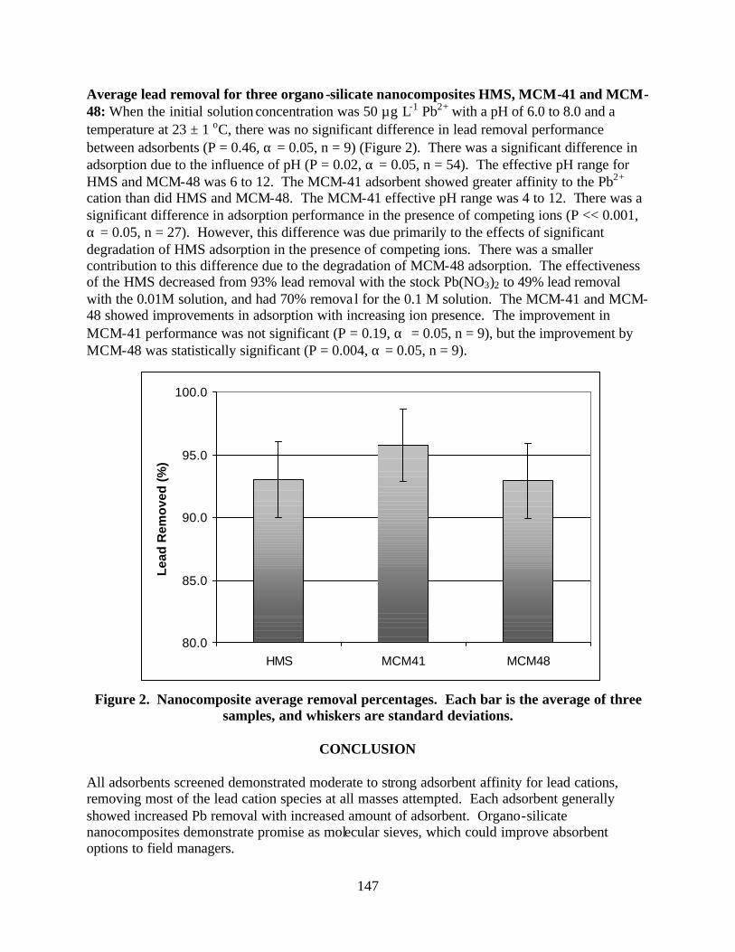
147

80.0

85.0

90.0

95.0

100.0

HMS MCM41 MCM48

Lea

d R

emo

ved

(%

)

Average lead removal for three organo-silicate nanocomposites HMS, MCM-41 and MCM-48: When the initial solution concentration was 50 µg L-1 Pb2+ with a pH of 6.0 to 8.0 and a temperature at 23 ± 1 oC, there was no significant difference in lead removal performance between adsorbents (P = 0.46, α = 0.05, n = 9) (Figure 2). There was a significant difference in adsorption due to the influence of pH (P = 0.02, α = 0.05, n = 54). The effective pH range for HMS and MCM-48 was 6 to 12. The MCM-41 adsorbent showed greater affinity to the Pb2+ cation than did HMS and MCM-48. The MCM-41 effective pH range was 4 to 12. There was a significant difference in adsorption performance in the presence of competing ions (P << 0.001, α = 0.05, n = 27). However, this difference was due primarily to the effects of significant degradation of HMS adsorption in the presence of competing ions. There was a smaller contribution to this difference due to the degradation of MCM-48 adsorption. The effectiveness of the HMS decreased from 93% lead removal with the stock Pb(NO3)2 to 49% lead removal with the 0.01M solution, and had 70% remova l for the 0.1 M solution. The MCM-41 and MCM-48 showed improvements in adsorption with increasing ion presence. The improvement in MCM-41 performance was not significant (P = 0.19, α = 0.05, n = 9), but the improvement by MCM-48 was statistically significant (P = 0.004, α = 0.05, n = 9).

Figure 2. Nanocomposite average removal percentages. Each bar is the average of three samples, and whiskers are standard deviations.

CONCLUSION

All adsorbents screened demonstrated moderate to strong adsorbent affinity for lead cations, removing most of the lead cation species at all masses attempted. Each adsorbent generally showed increased Pb removal with increased amount of adsorbent. Organo-silicate nanocomposites demonstrate promise as molecular sieves, which could improve absorbent options to field managers.

148

REFERENCES

Abdel-Fattah, T. and K. Payne. 2001. Screening of low-cost absorbents for lead removal. American Chemical Society. Preprints of Extended Abstracts. 41(1): 244. Caro, J., M. Noack, P. Kolsch and R. Schafer. 2000. Zeolite membranes – state of their development and perspective. Microporous and Mesoporous Materials 38(1): 3-24. Mellor, A. and C. McCartney. 1994. The effects of lead shot deposition on soils and crops at a clay pigeon shooting site in northern England. Soil Use and Management 10: 124-129. Pickering, W.F. 1986. Ore Geol. Rev. 1. 83-146. Cited in Rampley, C.G. and K. L. Ogden. 1998. Preliminary studies for removal of lead from surrogate and real soils using a water soluble chelator: adsorption and batch extraction. Environmental Science & Technology 32(7): 987-993.

149

SYSTEM DYNAMICS MODELING AS AN AID TO WATER SUPPLY PLANNING

Samuel H. Austin Virginia Department of Forestry

900 Natural Resources Drive, Suite 800, Charlottesville, VA 22903 austins@dof.state.va.us

KEY WORDS: modeling, feedback, system dynamics, water, planning

ABSTRACT Dry weather and drought during the past four years have heightened awareness of the need for accurate prediction and planning for human water needs. Traditional planning tools often overlook the feedback loops and non- linear rates of change embedded within the dynamics of population growth, water supply, and water consumption. This lack of awareness may lead to over estimates or under estimates of projected water demand and supply. System dynamics modeling can accurately capture and articulate the structure, causal loops, feedback, and non- linear dynamics that are part of natural systems. A system dynamics model can be a useful aid to managerial planning and scenario analysis. A system dynamics model is presented that characterizes water supply and demand at the watershed scale. The effects on supply and demand of population growth, change in land use, and change in impervious area may be simulated over time. The dynamics of user-defined management policy scenarios may be documented and compared over the mid-term and long term. The model may serve as a helpful aid to policy analysis and management decision-making.

INTRODUCTION We live in a world that organizes itself using processes that continuously change the states of ecosystem organization. The second law of thermodynamics combined with the negative (compensating) and positive (reinforcing) feedback links that control everything from thermostats to servomechanisms to tree growth to the human opposable thumb, ensure that change is endless and proceeding at rates that also change in non- linear fashion over time. States of ecosystem organization fluctuate with time. It makes sense then to model real world processes using methods that capture some of the richly dynamic ebb and flow of change in our world. System dynamics modeling is one method of doing this. The technique relies on an accurate characterization of the structure of a dynamic system needed to produce a certain reference behavior. A map showing structural links is created, equations are used to describe relationships among links, and computer simulation is used to “set things in motion,” allowing changes in system components, caused by other system components, to play out over time. With a useful representation of system structure in hand, past and future changes may be simulated, making system dynamics modeling an informative aid to management’s decision-making.

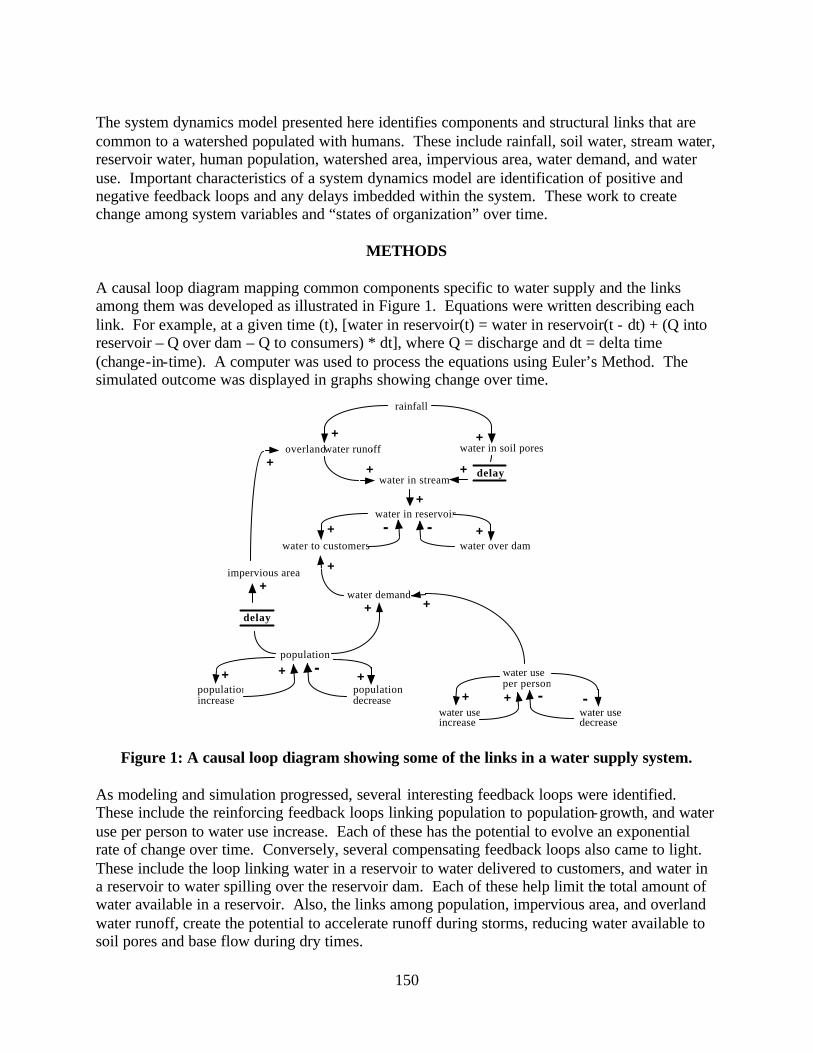
150

The system dynamics model presented here identifies components and structural links that are common to a watershed populated with humans. These include rainfall, soil water, stream water, reservoir water, human population, watershed area, impervious area, water demand, and water use. Important characteristics of a system dynamics model are identification of positive and negative feedback loops and any delays imbedded within the system. These work to create change among system variables and “states of organization” over time.

METHODS A causal loop diagram mapping common components specific to water supply and the links among them was developed as illustrated in Figure 1. Equations were written describing each link. For example, at a given time (t), [water in reservoir(t) = water in reservoir(t - dt) + (Q into reservoir – Q over dam – Q to consumers) * dt], where Q = discharge and dt = delta time (change-in-time). A computer was used to process the equations using Euler’s Method. The simulated outcome was displayed in graphs showing change over time.

Figure 1: A causal loop diagram showing some of the links in a water supply system.

As modeling and simulation progressed, several interesting feedback loops were identified. These include the reinforcing feedback loops linking population to population-growth, and water use per person to water use increase. Each of these has the potential to evolve an exponential rate of change over time. Conversely, several compensating feedback loops also came to light. These include the loop linking water in a reservoir to water delivered to customers, and water in a reservoir to water spilling over the reservoir dam. Each of these help limit the total amount of water available in a reservoir. Also, the links among population, impervious area, and overland water runoff, create the potential to accelerate runoff during storms, reducing water available to soil pores and base flow during dry times.

rainfall

water in soil poresoverland water runoff

water in reservoir

water in stream

water over damwater to customers

water demand

population

population increase

population decrease

water use per person

water use decrease

water use increase

impervious area

+

+

+

+

+

++

+

++

+

- -

+

+ + +-

+ + --

delay

delay

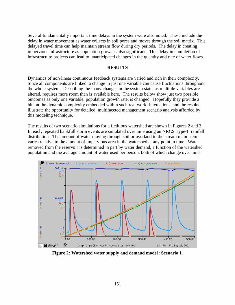
151

Several fundamentally important time delays in the system were also noted. These include the delay in water movement as water collects in soil pores and moves through the soil matrix. This delayed travel time can help maintain stream flow during dry periods. The delay in creating impervious infrastructure as population grows is also significant. This delay in completion of infrastructure projects can lead to unanticipated changes in the quantity and rate of water flows.

RESULTS Dynamics of non- linear continuous feedback systems are varied and rich in their complexity. Since all components are linked, a change in just one variable can cause fluctuations throughout the whole system. Describing the many changes in the system state, as multiple variables are altered, requires more room than is available here. The results below show just two possible outcomes as only one variable, population growth rate, is changed. Hopefully they provide a hint at the dynamic complexity embedded within such real world interactions, and the results illustrate the opportunity for detailed, multifaceted management scenario analysis afforded by this modeling technique. The results of two scenario simulations for a fictitious watershed are shown in Figures 2 and 3. In each, repeated bankfull storm events are simulated over time using an NRCS Type-II rainfall distribution. The amount of water moving through soil or overland to the stream main-stem varies relative to the amount of impervious area in the watershed at any point in time. Water removed from the reservoir is determined in part by water demand, a function of the watershed population and the average amount of water used per person, both of which change over time.

1:43 PM Fri, Sep 26, 2003

1.00 100.80 200.60 300.40 400.20 500.00

Months

1:

1:

1:

2:

2:

2:

3:

3:

3:

4:

4:

4:

5:

5:

5:

0

7515.68

15031.4

5.l

30.‡

55.‡

0

20.‡

40.‡

11.

15.5

20.‡

10

14

17

1: water in reservoir 2: Q into reservoir 3: Q over dam 4: Q to consumers 5: population

1 1 1 1 1

22 2 2

2

3 33 3 3

4

4

4

4

4

5

5

5

5

5

Graph 1: p1 (Sam Austin: Scenario 1) Figure 2: Watershed water supply and demand model: Scenario 1.

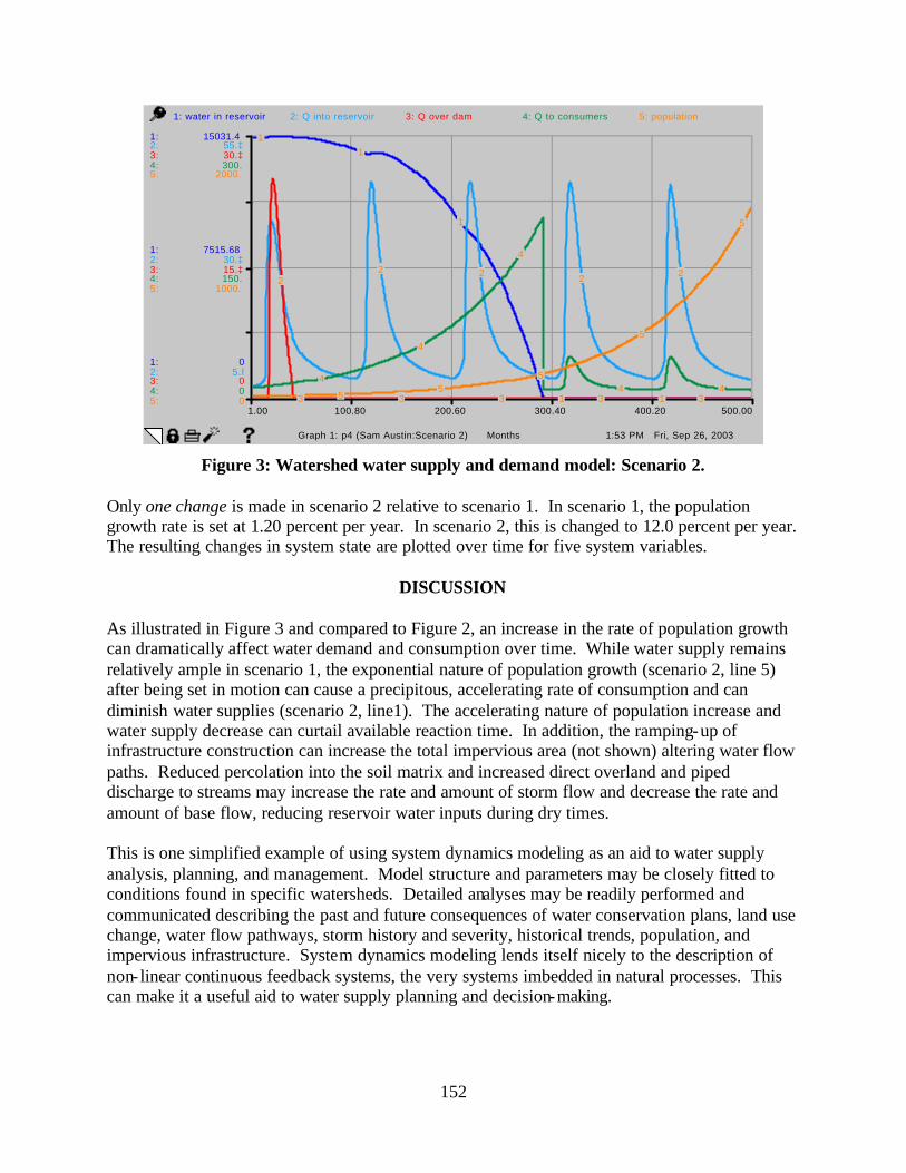
152

1:53 PM Fri, Sep 26, 2003

1.00 100.80 200.60 300.40 400.20 500.00

Months

1:

1:

1:

2:

2:

2:

3:

3:

3:

4:

4:

4:

5:

5:

5:

0

7515.68

15031.4

5.l

30.‡

55.‡

0

15.‡

30.‡

0

150.

300.

0

1000.

2000.

1: water in reservoir 2: Q into reservoir 3: Q over dam 4: Q to consumers 5: population

11

1

1 1

22 2 2 2

3 3 3 3 3

4

4

4

4 45

55

5

5

Graph 1: p4 (Sam Austin:Scenario 2) Figure 3: Watershed water supply and demand model: Scenario 2.

Only one change is made in scenario 2 relative to scenario 1. In scenario 1, the population growth rate is set at 1.20 percent per year. In scenario 2, this is changed to 12.0 percent per year. The resulting changes in system state are plotted over time for five system variables.

DISCUSSION As illustrated in Figure 3 and compared to Figure 2, an increase in the rate of population growth can dramatically affect water demand and consumption over time. While water supply remains relatively ample in scenario 1, the exponential nature of population growth (scenario 2, line 5) after being set in motion can cause a precipitous, accelerating rate of consumption and can diminish water supplies (scenario 2, line1). The accelerating nature of population increase and water supply decrease can curtail available reaction time. In addition, the ramping-up of infrastructure construction can increase the total impervious area (not shown) altering water flow paths. Reduced percolation into the soil matrix and increased direct overland and piped discharge to streams may increase the rate and amount of storm flow and decrease the rate and amount of base flow, reducing reservoir water inputs during dry times. This is one simplified example of using system dynamics modeling as an aid to water supply analysis, planning, and management. Model structure and parameters may be closely fitted to conditions found in specific watersheds. Detailed analyses may be readily performed and communicated describing the past and future consequences of water conservation plans, land use change, water flow pathways, storm history and severity, historical trends, population, and impervious infrastructure. System dynamics modeling lends itself nicely to the description of non- linear continuous feedback systems, the very systems imbedded in natural processes. This can make it a useful aid to water supply planning and decision-making.

153

REFERENCES Boyce, S.G. 1985. Forestry Decisions. Gen Tech. Rep, S.E. 35, USDA Forest Service, Southeastern Forest Experiment Station. Asheville, N.C. Forrester, Jay W. 1961. Industrial Dynamics. Productivity Press. Cambridge, Mass. Forrester, Jay W. 1976. Urban Dynamics. MIT Press. Cambridge, Mass. Kuhn, Thomas S. 1962. The Structure of Scientific Revolutions. The University of Chicago Press. Chicago, Ill. Lyneis, James M. 1980. Corporate Planning and Policy Design. Pugh-Roberts Associates, Inc. Cambridge, Mass. Meadows, Donella H. 1972. The Limits to Growth. Universe Books. New York, N.Y. Meadows, Donella H. 1982. Groping In The Dark: The First Decade of Global Modeling. John Wiley and Sons. New York, N.Y. Meadows, Donella H. 1991. The Global Citizen. Island Press. Washington, D.C. Meadows, Dennis L. - Editor. 1973. Toward Global Equilibrium: Collected Papers. Wright-Allen Press. Cambridge, Mass. Meadows, Dennis L. 1974. Dynamics of Growth In A Finite World. Wright-Allen Press. Cambridge, Mass. Morecroft and Sterman. 1994. Modeling for Learning Organizations. Productivity Press, Portland, Ore. Randers, Jorgen (Editor). 1980. Elements of the System Dynamics Method. MIT Press. Cambridge, Mass. Richardson, George P. and A. L. Pugh, III. 1981. Introduction to System Dynamics Modeling with DYNAMO. MIT Press. Portland, Ore. Senge, Peter M. 1990. The Fifth Discipline. Doubleday Currency. New York, N.Y. Senge, Peter M. 1994. The Fifth Discipline Fieldbook. Doubleday Currency. New York, N.Y.

154

REGIONAL WATER RESOURCE PLANNING – AN EXAMPLE FROM THE CENTRAL COASTAL PLAIN CAPACITY USE AREA OF NORTH CAROLINA

Brent Waters

Golder Associates Inc. 3701 Saunders Avenue, Richmond, VA 23227

Jean Crews-Klein

Natural Resources and Economic Development North Carolina Rural Economic Development Center, Inc.

4021 Carya Drive, Raleigh, NC 27610 KEY WORDS: groundwater, water supply, regional planning

ABSTRACT In August 2002, North Carolina passed the Central Coastal Plain Capacity Use Area (CCPCUA) Rule to regulate groundwater withdrawal from Cretaceous aquifers. The goal of the rule is to minimize serious water level declines and salt water intrusion that have been progressively worsening in these aquifers. The major groundwater impacts are being observed in two principal aquifers, Black Creek and Upper Cape Fear, which have been desirable sources of high-quality, low-cost drinking water throughout a 15-county region. The regulations require groundwater withdrawals from the most affected portions of the region to be limited to 1997 withdrawal rates and may be further reduced by up to 75% over a 16-year period ending in 2018. The regulations are meant to avoid permanent damage to the aquifers and to help support economic growth in the region by having a sustainable water supply through the development of alternative water supplies and by promoting water conservation and reuse. The North Carolina Rural Economic Development Center undertook a study to determine the effects of the CCPCUA Rule, evaluate current and future water supply needs and sources, identify water supply alternatives, and estimate the costs of compliance for 122 public water supply systems affected by this rule. The regional water-resource study was made possible due to comprehensive local water supply planning efforts required by North Carolina. Local governments that operate public water systems are required to submit Local Water Supply Plans (LWSP) every 5 years. These plans provide an assessment of a water system's current and future water needs and provide a valuable tool for local governments to better manage water supplies and plan for water supply system improvements needed to meet future water supply demand. The LWSPs are prepared by each local government and submitted to the state government, where data are compiled into a massive electronic database and geographic information system. The existence of this local water supply planning data allows analysis of current and future water supply needs, water system infrastructure, and available water resources on a regional scale. It also greatly facilitated the CCPCUA Regional Water Resource Study. If fully implemented, the CCPCUA Rule will impact over 40 public water systems and will result in the elimination of 38 million gallons per day of existing groundwater sources. The

155

replacement of these sources and development of alternative water supplies to meet future 2020 water demand is estimated to cost more than $250 million. Alternative water sources identified by the study include: 1) development of alternate groundwater supplies from underutilized aquifers; 2) development of surface water sources; 3) regionalization of water systems to allow more efficient use of existing water supplies; 4) water conservation, demand reduction, and water reuse; and 5) non-traditional sources such as brackish water, mine dewatering supplies, horizontal collector wells, and aquifer storage and recovery. Regional cooperation will be an important opportunity, allowing economy of scale in addressing aggregate demand, cost sharing, uniform rates, and bond- issuing authority.

156

THE USE OF GRAY WATER AS A WATER CONSERVATION METHOD

Judy A. Poff Virginia Water Resources Research Center

23 Agnew Hall, Blacksburg, VA 24061 jupoff@vt.edu

KEYWORDS: gray water, conservation, water reuse

INTRODUCTION Using gray water has been a long-standing, controversial conservation method in water-starved states such as California, Arizona, Florida, and parts of Texas. In 1998, the Virginia General Assembly addressed this subject by passing legislation on the use of rainwater and reuse of gray water (See Virginia Code 32.1-248.2). This legislation directed the Virginia Department of Health (VDH) to develop guidelines by January 1, 1999 that define gray water and the conditions under which gray water could be used and for what purposes. In addition, the General Assembly directed the VDH to work in conjunction with the Department of Environmental Quality to promote the use of rainwater and reuse of gray water as a means to reduce fresh water consumption, ease demands on public treatment works and water supply systems, and promote conservation.

WHAT IS GRAY WATER? The definition of gray water varies from state to state as do the regulations governing its use. Generally, the wastewater from the shower, bathtub, bathroom basin, and laundry water (unless it is exposed to soiled diapers) is considered gray water. However, some states include rinse water from the dishwasher and kitchen sink (as long as the water has not come in contact with poultry or meat products). Water coming from the kitchen sink, toilets, and urinals is considered black water and should be properly disposed through the residential waste disposal system. In addition, if someone with an infectious disease lives in the home, all wastewater that emanates from the daily care of the individual should be considered black water and disposed through the waste disposal system.

HOW SAFE IS GRAY WATER? Gray water is wastewater. As such, it contains bacteria and organisms that can cause illness if not properly handled and treated. Few long-term studies have been completed to determine the effects of gray water use on human health. Because each household is different, the quality and quantity (Table 1) of gray water depends on many factors such as the age and health of the household occupants, standard of living, and daily activities. If the gray water system is properly designed and the water is treated appropriately, then the risk of contamination is greatly reduced. Gray water needs to be disinfected within three hours of storage time. Routine inspection of the system is critical to prevent the spread of such diseases as typhoid fever, dysentery, hepatitis, and other bacterial and viral diseases. Studies have shown that when children and pets are present in

157

the household, generally the total and fecal coliform numbers are higher (Gerba et. al. 1995). When kitchen sink water is added to the mixture, the levels of fecal coliform are higher in soil that has been irrigated with graywater (WCASA 2001).

Table 1. Indoor water use for an average household.

Amount (gallons Per capita per day, gcd)

Source

15.0 Washing machine 18.5 Toilet 12.8 Shower, bath 10.9 Sinks, faucet 9.5 Leaks

1.0 Dishwasher 1.6 Other uses 69.3 Total indoor water use

*1999 AWWA Research Foundation and American Water Works Association

The Swedish Study: The study most often sited by researchers has been termed the Classic Swedish Study by Karlgren, Tullander, Ahl, and Olsen (1967). The Swedish National Board for Building and Research funded the study of a multi-apartment complex in Stockholm with plumbing that separated gray water from blackwater. This study took place over a 12-week period and looked at the BOD5 (five-day biological oxygen demand) and the chemical oxygen demand (COD) of wastewaters (gray and black water). It was found that gray water decomposes much faster than black water, is about 10 to 15 degrees warmer than normal wastewater, and contains high levels of grease, fiber, and particulates. Treating gray water before it reaches its toxic state (can be as short as 3 hours) is important to reduce the risk of pollution. Table 2, taken from the Swedish study (Karlgren et al. 1967) gives the test results for the water samples taken from the households in the apartment complex. WCASA Study: A more recent study by the Water Conservation Alliance of Southern Arizona (WCASA 2001) assessed the risks of gray water reuse using eleven Tucson, Arizona households as study sites for a 12-month period. The researchers analyzed gray water, gray water irrigated soils, and potable water irrigated soils for fecal coliforms, fecal streptococci, and Escherichia coli. Research results indicated that gray water that included water from the kitchen sink had higher levels of fecal coliforms than gray water that did not include water from the kitchen sink. Also, gray water kept in underground storage tanks had higher levels of fecal coliforms than did gray water that was not stored underground. Children and pets in the home made a small difference in the coliform count. For a complete description of the methodology and findings, see CASA’s website: www.watercasa.org/research/residential.analysis.htm.

158

Table 2: Quantity and relative pollution in gray water and black water.

Analysis Graywater Blackwater Gray+Black Grayw. % Blackw. % BOD5 g/p.d 25 20 45 56 % 44 % COD g/p.d 48 72 120 40 % 60 % Total Phos.g/p.d 2.2 1.6 3.5 58 % 42 % Kjeldahl N g/p.d 1.1 11 12.1 9 % 91 % Total Residue g/p.d 77 53 130 58 % 41 % Fixed Tot. Res. g/p.d 33 14 47 70 % 30 % Volatile T.R. g/p.d 44 39 83 53 % 47 % Nonfilterable g/p.d 18 20 48 38 % 62 % Fixed NonFilt. g/p.d 3 5 8 38 % 62 % Volatile Nonfilterable g/p.d 15 25 40 38 % 62 % Plate c 35ª 83x10e9 62x10e9 145x10e9 57 % 43 % Coli 35º 8.5x10e9 4.8x10e9 13x10e9 64 % 36 % Coli 44º 1.7x10e9 3.8x10e9 6x10e9 31 % 69 % Effluent flow (liters) 121.5 8.5 130 93 % 7 %

g/pd=gram/person.day(24h) Ultra low-flush vacuum toilet

Information for this table was taken from Carl Lindstrom, website www.greywater.com/pollution.htm.

VIRGINIA’S GUIDELINES Homeowners installing a gray water system in a private dwelling must first seek a permit issued by the State Health Commissioner. This permit must be obtained prior to the installation and use of the gray water system. Plumbing fixtures used in a gray water system must comply with the requirements of the statewide building code and all applicable state and local regulations and policies implemented through the Virginia Department of Health. A copy of the gray water guidelines may be obtained from the local health department or the state VDH. Figure 1 shows the typical design of a gray water system. Under Virginia’s guidelines, all components of the gray water system must be designed and certified by an appropriately licensed professional consultant or certified as to treatment performance by a nationally recognized testing authority such as the National Sanitation Foundation (NSF). Prior to the operation of a newly installed gray water system, it must be approved by the local and state health department staff.

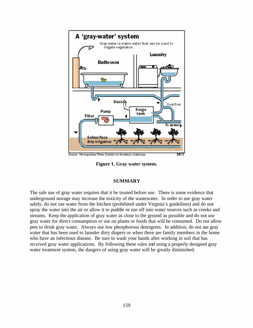
159

Figure 1. Gray water system.

SUMMARY The safe use of gray water requires that it be treated before use. There is some evidence that underground storage may increase the toxicity of the wastewater. In order to use gray water safely, do not use water from the kitchen (prohibited under Virginia’s guidelines) and do not spray the water into the air or allow it to puddle or run off into water sources such as creeks and streams. Keep the application of gray water as close to the ground as possible and do not use gray water for direct consumption or use on plants or foods that will be consumed. Do not allow pets to drink gray water. Always use low phosphorous detergents. In addition, do not use gray water that has been used to launder dirty diapers or when there are family members in the home who have an infectious disease. Be sure to wash your hands after working in soil that has received gray water applications. By following these rules and using a properly designed gray water treatment system, the dangers of using gray water will be greatly diminished.

160

REFERENCES Gerba, C. P., T. M. Straub, J. B. Rose, M.M. Karpiscak, K.E. Foster, and R. G. Brittain. 1995. Water Quality Study of Graywater Treatment Systems. AWRA Paper Number 94081, Vol. 32, No. 1, February. pp. 109-116. Karlgren, L., Victor Tullander, Torsten Ahl and Eskil Olson. 1967. Residential waste water (Hushållsspillvattnet). Water (Vatten) March: 3-67. Lindstrom, C. Greywater pollution. www.greywater.com/pollution.htm (January 15, 2004). Water Conservation Alliance of Southern Arizona (WCASA). 2001. Residential Graywater Reuse Study. www.watercasa.org/research/residential/analysis.htm (January 15, 2004).

161

THE INFLUENCE OF RESIDENTIAL WATER CONSERVATION PROGRAMS: APPLICATIONS FOR VIRGINIA

Kurt Stephenson

Department of Agricultural and Applied Economics, Virginia Tech Hutcheson Hall, Blacksburg, VA 24061

Lauren Cartwright

Institute for Water Resources 7701 Telegraph Road, Alexandria, VA 22315 Lauren.A.Cartwright@wrc01.usace.army.mil

KEY WORDS: water conservation, policy, incentives

ABSTRACT Recent droughts and the ensuing strains on water supply sources have highlighted the interest in water conservation policies in Virginia. The lack of technical information regarding the influence of water conservation programs on residential water demand is a continuing challenge for water planners. This presentation reviews the current state of the knowledge about the effectiveness of various water conservation policies in the mid-Atlantic region. The presentation also highlights the results of a study on the influence of imposition of conservation programs on residential water customers in Stafford County, Virginia based on a decade of historical data.

INTRODUCTION Water conservation describes a broad array of policies that a water supply manager can use to encourage reductions in per capita water demand. Conservation programs are categorized into three groups for discussion: financial, regulatory, and educational. A locality may choose to use any one or a combination of approaches to achieve long-term conservation goals or short-term drought curtailment goals. Empirical information on the expected level of response from the imposition of different approaches to water conservation is important to effective water supply planning. Financial incentives rely on monetary enticements to encourage water conservation. Financial incentives include: conservation rate structures and rate increases, rebates for installing water saving technology (such as low flush toilets), and fees on water use above a specified level. Conservation rate structures and price increases are a common form of financial incentive imposed by water utilities. Regulatory incentives encourage water conservation by imposing mandatory rules on when and how customers can use water or what types of water using appliances are acceptable (such as low flush toilets and low flow showerheads). Regulatory incentives include irrigation scheduling, water efficient plumbing codes, and standards for landscape design. Within this group of incentives, the most technical information available is long-term conservation as a result of the national plumbing standards regulations imposed in 1994 by the US Energy Policy Act (EPAct). EPAct regulated that low flush toilets and low flow

162

showerheads and faucets had to be installed in new houses built after January 1, 1994. Educational incentives educate consumers about ways to conserve water and the importance of water conservation. Educational incentives include television and radio ads, direct mail literature, and school programs.

METHODS This paper provides a synthesis of what is known about the effectiveness of these three types of water conservation programs in reducing water demand. The synthesis is developed by first summarizing previous research on water conservation. Second, the paper reports on a statistical study of the effectiveness of water conservation programs in Stafford County, Virginia (Cartwright 2002). The Stafford County study examines whether residential water use in Virginia changed due to changes in regulatory, financial, and educational water conservation programs. In 1995, Stafford changed from a decreasing block rate structure to an increasing block rate structure with additional pricing incentives to reduce peak summer use. Stafford County has also witnessed a 32 percent increase in the number of new connections between 1994 and 2000. The rapid growth in the new connections can provide empirical evidence as to whether the new plumbing standards have resulted in a structural shift in household water demand. Finally, Stafford County implemented a voluntary educational conservation campaign during the summer of 1999 to reduce residential water use. The Stafford County study provides state-specific results that add to the insights gained from the literature review.

RESULTS AND DISCUSSION Studies show price increases and conservation rate structures typically encourage water conservation, especially in the long term and summer months when water demand is more discretionary (Espey et al. 1997). An analysis of 124 estimates of price elasticity from the literature shows the mean of the price elasticity estimates is –0.41 (median of –0.35, and standard deviation of 0.86) (Dalhuisen et al. 2003). Therefore, although on average price elasticity is relatively inelastic, residential water customers are responsive to price increases. However, the analysis of Stafford County water demand shows that the imposition of financial incentives does not guarantee a reduction in per capita water consumption. No statistical evidence was found that the imposition of a new Stafford water rate structure in 1995 produced a measurable change in residential water consumption. This unexpected result in the Stafford study might be explained in two ways. First, Stafford residential water consumption (measured in per capita consumption) is already relatively low compared with estimates in Virginia and the southeastern U.S. as a whole (Malcolm Pirnie, Inc. 2001). This relatively low level of consumption leaves little room for customers to further reduce water demand by a measurable amount. An alternative explanation for the lack of responsiveness to financial incentives is that the new water rates in Stafford, while higher than the previous rates, were still too low to elicit a significant change in water use behavior. The literature suggests that EPAct plumbing standards have a significant impact on residential water demand. Although precise relationships are difficult given the long-term nature of the changes, studies have estimated that one low flush toilet decreases monthly household water demand by 10 to 11 percent, and one low flow showerhead decreases monthly household water

163

demand by 2 to 9.7 percent (Renwick and Archibald 1998). However, challenges in separating and identifying long-term changes in water demand were demonstrated in the Stafford study. Stafford County’s per household water demand has not changed appreciably over the past decade despite a rapidly increasing percentage of the housing stocked with new plumbing standards. In an economy with increasing median household incomes, the demand reduction from plumbing standards may be offset by increases in household water demand associated with higher income households (due to luxury items such as swimming pools and automatic sprinkler systems). Little systematic empirical analysis exists on the responsiveness of customers to conservation programs utilizing educational incentives (Michelsen et al. 1999). However, a recent California study found measurable levels of demand reduction due to the imposition of educational incentives. Although generalizations made between California and Virginia may be problematic, the results of the California study do provide empirical evidence that utilities can achieve some reductions in water use through educational programs (Renwick and Green 2000). The Stafford analysis, however, found no statistical evidence that a short-term education program to discourage water use during a dry summer in 1999 significantly reduced per capita water consumption.

CONCLUSION The imposition of financial and regulatory conservation incentives has the greatest potential for achieving water conservation goals, both long term and short term, in Virginia versus educational incentives. Empirical evidence suggests that responsiveness to financial incentives is greater in the long term and in the summer months. However, financial incentives may not result in a measurable level of residential water conservation if customers are not able to perceive the rate change or already consume water at a relatively low level. Measurable reductions in water use due to the national EPAct standards shows that retrofit activities through local regulatory incentives have the potential to significantly conserve water. However, in economies experiencing increasing median household incomes, any conservation due to retrofit activities may be offset by high water use for luxury items. Virginia localities should not expect educational incentives alone to achieve water conservation goals. However, the use of educational incentives as part of a conservation program should not be underestimated. Educational incentives inform customers of the need for conservation and potentially increase the response to regulatory and financial incentives.

ACKNOWLEDGMENTS

Thanks to Bob Bos, Stafford Water Utilities Manager, for providing the data for the study of Stafford residential water demand. The Rappahannock River Basin Commission provided partial funding for this study.

164

REFERENCES

Cartwright, L.A. 2002. The Influence of Conservation Programs on Residential Water Demand: Synthesis and Analysis for Shared Vision Planning in the Rappahannock River Basin. M.S. Thesis. Department of Agricultural and Applied Economics, Virginia Tech. Blacksburg, Va. Dalhuisen, J.M., R. Florax, H. de Groot, and P. Nijkamp. 2003. Price and income elasticities of residential water demand: A meta-analysis. Land Economics 79(2): 292-308. EPAct. Energy Policy Act of 1992, Public Law 102-486, 106 Stat. 2776, 102d Congress, Oct. 24, 1992. Espey, M., J. Espey, and W.D. Shaw. 1997. Price elasticity of residential demand for water: A meta analysis. Water Resources Research 33(6): 1369-1374. Malcolm Pirnie, Inc. 2001. Environmental Impact Report for the Rocky Pen Run Reservoir Project: Stafford County, Virginia. Revised Section 2.0 (Purpose and Need for Action). Newport News, Va. Michelsen, A. M., J.T. McGuckin and D. Stumpf. 1999. Nonprice water conservation programs as a demand management tool. Journal of the American Water Resources Association 35(3): 593-602. Renwick, M. E. and S. O. Archibald. 1998. Demand side management policies for residential water use: Who bears the conservation burden? Land Economics 74(3): 343-359. Renwick, M. E. and R.D. Green. 2000. Do residential water demand side management policies measure up? An analysis of eight California water agencies. Journal of Environmental Economics and Management 40: 37-55.

165

INFLUENCE OF THE CHESAPEAKE BAY IMPACT STRUCTURE ON GROUNDWATER FLOW AND SALINITY

Charles E. Heywood

U.S. Geological Survey 1730 E. Parham Road, Richmond, VA, 23228

cheywood@usgs.gov

KEY WORDS: groundwater, simulation, impact structure, salinity, variable-density flow

ABSTRACT A preliminary three-dimensional variable-density groundwater flow model of the Virginia Coastal Plain aquifer system was constructed to investigate the occurrence of saltwater in the area of the Chesapeake Bay Impact Crater. Anomalously high salinities are observed in and around the crater, which is filled with low-permeability tsunami deposits. Simulations support the idea that preferential flushing occurred through hydraulically conductive parts of the aquifer system, while salt water was retained in low-permeability areas, including the crater fill. The persistence of saltwater within the crater throughout the Pleistocene places an upper bound on the effective hydraulic conductivity of the tsunami-breccia. Appreciable pumping stress is occurring in southeastern Virginia; consideration of miscible, density-dependent flow in this area improves the accuracy and potential usefulness of the groundwater model as a management tool.

INTRODUCTION Multiple marine transgressions and regressions since the Cretaceous Period have deposited a sequence of unconsolidated marine sands and clays over Cretaceous fluvial-deltaic sediments in the Atlantic Coastal Plain of eastern Virginia. Approximately 35 million years ago, an asteroid or comet impact disrupted Lower Cretaceous through Middle Eocene sediments near the mouth of the present day Chesapeake Bay (Poag et al. 1994). Cederstrom (1943) mapped the distribution of dissolved solids in ground water in the Atlantic Coastal Plain of Virginia, and noted an “inland wedge” of anomalously high concentration near the southern Chesapeake Bay (Figure 1). The near coincidence of the Chesapeake Bay impact structure suggests geologic control of the observed salinity distribution (Powars and Bruce 1999). Chemical analyses of ground water indicate a pre-Pleistocene seawater source of salt within the impact structure (McFarland 2002). Brine within the crater may have formed by heating of the crater- fill slurry following impact (Sanford 2003) and would therefore be of a similar age as the crater. The persistence of saltwater within the crater through the Pleistocene, and possibly since the Eocene, suggests that low permeability of crater- fill sediments and small hydraulic gradients prevented fresh-water flushing across the impact structure. The sequence of lower Cretaceous to Holocene sands and clays, which dip and thicken to the east, comprise the Coastal Plain aquifer system in Virginia. Consolidated lower Mesozoic rift-basin and older crystalline bedrock west of the fall line (the western extent of the Coastal Plain aquifer system) extend eastward at depth and underlie the unconsolidated Coastal Plain

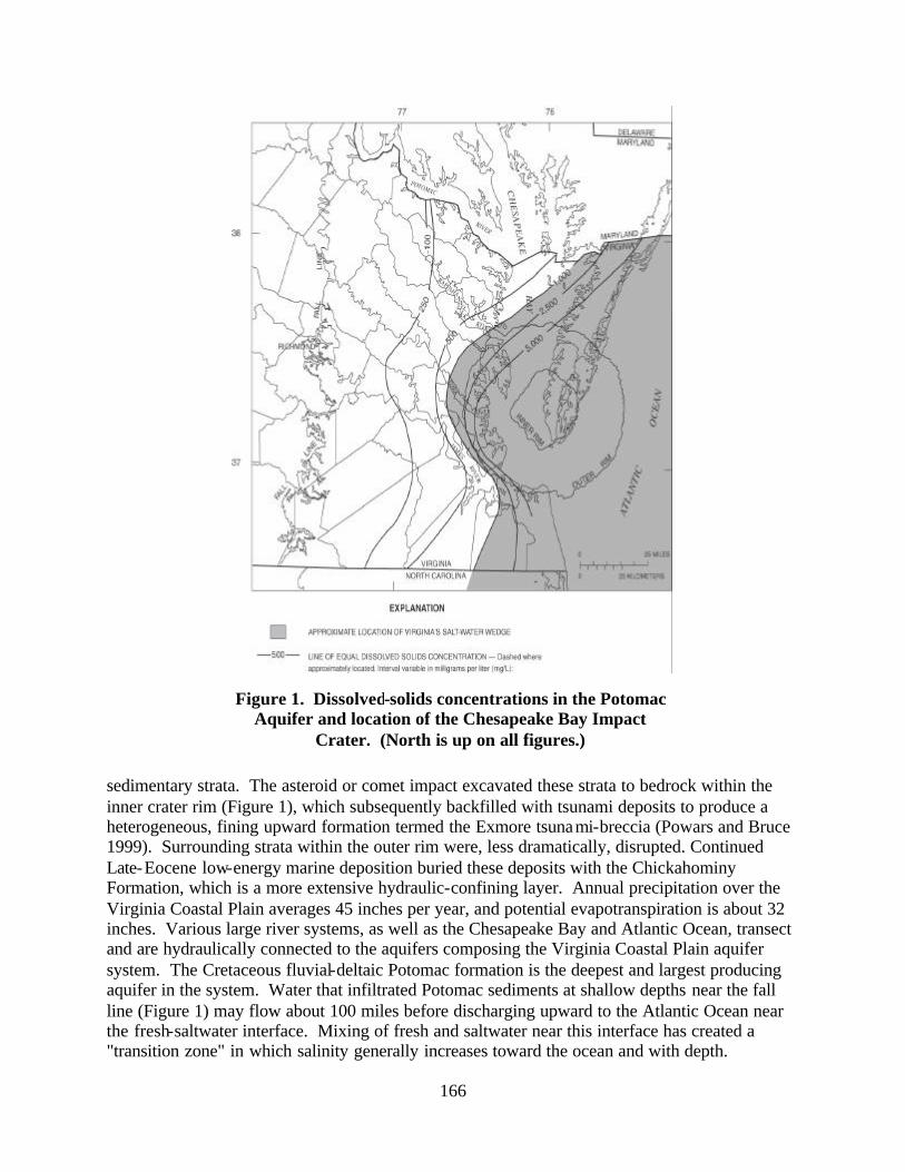
166

Figure 1. Dissolved-solids concentrations in the Potomac Aquifer and location of the Chesapeake Bay Impact

Crater. (North is up on all figures.)

sedimentary strata. The asteroid or comet impact excavated these strata to bedrock within the inner crater rim (Figure 1), which subsequently backfilled with tsunami deposits to produce a heterogeneous, fining upward formation termed the Exmore tsunami-breccia (Powars and Bruce 1999). Surrounding strata within the outer rim were, less dramatically, disrupted. Continued Late-Eocene low-energy marine deposition buried these deposits with the Chickahominy Formation, which is a more extensive hydraulic-confining layer. Annual precipitation over the Virginia Coastal Plain averages 45 inches per year, and potential evapotranspiration is about 32 inches. Various large river systems, as well as the Chesapeake Bay and Atlantic Ocean, transect and are hydraulically connected to the aquifers composing the Virginia Coastal Plain aquifer system. The Cretaceous fluvial-deltaic Potomac formation is the deepest and largest producing aquifer in the system. Water that infiltrated Potomac sediments at shallow depths near the fall line (Figure 1) may flow about 100 miles before discharging upward to the Atlantic Ocean near the fresh-saltwater interface. Mixing of fresh and saltwater near this interface has created a "transition zone" in which salinity generally increases toward the ocean and with depth.

167

However, preferential flow and flushing through conductive strata in some areas has resulted in more saline groundwater overlying fresher groundwater. Aquifers overlying the Potomac formation are similarly recharged where they outcrop to the west, and also leak through intervening clay confining units. The equilibrium location of the fresh-saltwater interface is primarily controlled by the sea level. It is also affected by the magnitude and distribution of recharge as well as the aquifer and confining-unit permeabilities. The Coastal Plain aquifers were entirely inundated and likely saturated with saltwater most recently during the Pliocene Epoch 1.6 million years ago, and numerous sea level changes have occurred since that time. The magnitude of relative sea level lowering during even the most recent glacial episode is uncertain, however. The ICE-4G model (Peltier 1994), which incorporates mantle viscosity and lithospheric flexure, computes sea level during the last glacial maximum (21,000 years before present) at 470 feet lower than present for the Virginia Coastal Plain. Age dating of basal peat below salt marshes and estuarine sediments in the Chesapeake Bay indicates sea level was 25 feet lower 6,000 years ago (Larsen and Clark 2003), which is about one-third of the ICE-4G model value for that time. During glacial episodes when the sea receded to the continental-shelf-slope break, the average aquifer-system hydraulic gradient may have been two to four times greater than with the current sea level, causing enhanced flushing of saltwater from aquifers and a seaward migration of the fresh-saltwater transition zone. Repeated sea level fluctuations during the late Tertiary and Quaternary have mixed freshwater with seawater, widening the fresh-saltwater transition zone (Meisler et al. 1984). The general trend of sea level rise over the past 18,000 years suggests that hydraulic forces affecting the location of the fresh-saltwater interface may be out of equilibrium, causing landward migration of the transition zone. The objective of this study was to quantitatively investigate the distribution and persistence of saltwater around the impact structure.

METHOD

Variable dissolved-solid concentrations can affect groundwater densities, and consequently groundwater flow. Groundwater systems without appreciable chemical reactions or temperature gradients are governed by equations for variable-density flow:

( )tC

CtP

pSsqq∂∂

∂ρ∂θ+

∂∂ρ=ρ+ρ⋅∇−

ϖ and mass transport: ( ) sCsqCqCD

tC

θ−

θ⋅∇−∇⋅∇=

∂∂

ϖ

where: ∇ is the gradient operator, ρ is the fluid density [ML-3], q

ϖis the specific discharge [LT-1],

P is the fluid pressure [ML-1T-2], Sp is the specific storage in pressure terms [M-1LT2], t is time [T], θ is the effective porosity, C is the solute concentration [ML-3], D is the dispersion coefficient [L2T-1], sq is the flow rate per unit volume representing sources or sinks [T-1], ρ is the source or sink fluid density [ML-3], sC is the source or sink solute concentration [ML-3].

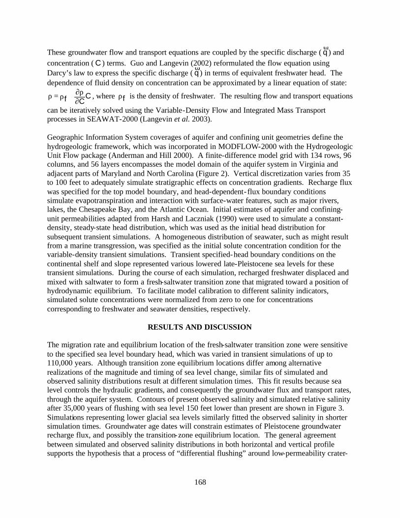
168

These groundwater flow and transport equations are coupled by the specific discharge ( qϖ

) and concentration ( C ) terms. Guo and Langevin (2002) reformulated the flow equation using Darcy’s law to express the specific discharge ( q

ϖ) in terms of equivalent freshwater head. The

dependence of fluid density on concentration can be approximated by a linear equation of state:

CCf ∂ρ∂+ρ=ρ , where ρf is the density of freshwater. The resulting flow and transport equations

can be iteratively solved using the Variable-Density Flow and Integrated Mass Transport processes in SEAWAT-2000 (Langevin et al. 2003). Geographic Information System coverages of aquifer and confining unit geometries define the hydrogeologic framework, which was incorporated in MODFLOW-2000 with the Hydrogeologic Unit Flow package (Anderman and Hill 2000). A finite-difference model grid with 134 rows, 96 columns, and 56 layers encompasses the model domain of the aquifer system in Virginia and adjacent parts of Maryland and North Carolina (Figure 2). Vertical discretization varies from 35 to 100 feet to adequately simulate stratigraphic effects on concentration gradients. Recharge flux was specified for the top model boundary, and head-dependent- flux boundary conditions simulate evapotranspiration and interaction with surface-water features, such as major rivers, lakes, the Chesapeake Bay, and the Atlantic Ocean. Initial estimates of aquifer and confining-unit permeabilities adapted from Harsh and Laczniak (1990) were used to simulate a constant-density, steady-state head distribution, which was used as the initial head distribution for subsequent transient simulations. A homogeneous distribution of seawater, such as might result from a marine transgression, was specified as the initial solute concentration condition for the variable-density transient simulations. Transient specified-head boundary conditions on the continental shelf and slope represented various lowered late-Pleistocene sea levels for these transient simulations. During the course of each simulation, recharged freshwater displaced and mixed with saltwater to form a fresh-saltwater transition zone that migrated toward a position of hydrodynamic equilibrium. To facilitate model calibration to different salinity indicators, simulated solute concentrations were normalized from zero to one for concentrations corresponding to freshwater and seawater densities, respectively.

RESULTS AND DISCUSSION

The migration rate and equilibrium location of the fresh-saltwater transition zone were sensitive to the specified sea level boundary head, which was varied in transient simulations of up to 110,000 years. Although transition zone equilibrium locations differ among alternative realizations of the magnitude and timing of sea level change, similar fits of simulated and observed salinity distributions result at different simulation times. This fit results because sea level controls the hydraulic gradients, and consequently the groundwater flux and transport rates, through the aquifer system. Contours of present observed salinity and simulated relative salinity after 35,000 years of flushing with sea level 150 feet lower than present are shown in Figure 3. Simulations representing lower glacial sea levels similarly fitted the observed salinity in shorter simulation times. Groundwater age dates will constrain estimates of Pleistocene groundwater recharge flux, and possibly the transition-zone equilibrium location. The general agreement between simulated and observed salinity distributions in both horizontal and vertical profile supports the hypothesis that a process of “differential flushing” around low-permeability crater-

169

Figure 2. Location of Chesapeake Bay Impact Crater and finite-difference model grid in Virginia and adjacent parts of Maryland and North Carolina.

0 10 20 30 40 50Miles

fill material caused the “inland wedge” of saltwater observed beneath the Virginia Coastal Plain. Hydraulically conductive parts of the aquifer system were flushed of saltwater, leaving remnant saltwater in low permeability areas, such as the crater fill. This process is more consistent with geochemical evidence and simpler than alternative salinity emplacement hypotheses, such as membrane filtration or halite dissolution. The lithology of the Exmore tsunami-breccia is highly variable, and laboratory hydraulic-conductivity measurements of Exmore tsunami-breccia core samples conducted by the U.S. Army Corps of Engineers range from 6x10-5 to 3 ft/day. Samples of the Exmore tsunami-breccia matrix and Chickahominy Formation have hydraulic conductivities of 10-3 or less; the higher values are from relatively undisturbed Exmore tsunami-breccia sand clasts (Randy McFarland, U.S. Geological Survey, written communication, 2002). The interconnectedness of the higher permeability Exmore tsunami-breccia lithologies is speculative but determines the larger-scale effective hydraulic conductivity of the formation. The simulated persistence of saltwater in the Exmore tsunami-breccia sediments for more than 100,000 years bounds the effective hydraulic conductivity to less than 10-3 ft/day for those sediments shallower than about 1,800 feet below modern sea level, where vigorous Pleistocene glacial flushing occurred. Deeper sediments resided in more stagnant ground water where less flushing occurred, even if clast-supported Exmore tsunami-breccia facies had higher hydraulic conductivity. Fault movement around the crater margin may also have locally decreased conductivities, creating effective barriers to flow.

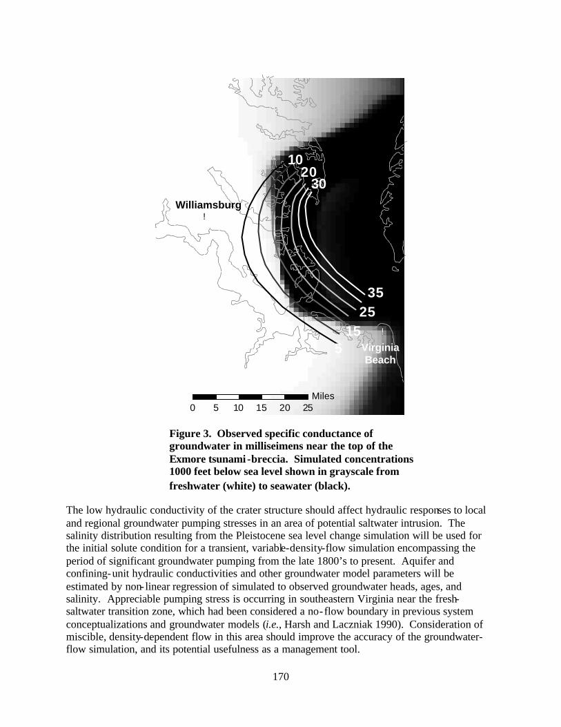
170

5

10

15

20

25

30

35

Williamsburg!

VirginiaBeach

!

0 5 10 15 20 25Miles

The low hydraulic conductivity of the crater structure should affect hydraulic responses to local and regional groundwater pumping stresses in an area of potential saltwater intrusion. The salinity distribution resulting from the Pleistocene sea level change simulation will be used for the initial solute condition for a transient, variable-density-flow simulation encompassing the period of significant groundwater pumping from the late 1800’s to present. Aquifer and confining-unit hydraulic conductivities and other groundwater model parameters will be estimated by non- linear regression of simulated to observed groundwater heads, ages, and salinity. Appreciable pumping stress is occurring in southeastern Virginia near the fresh-saltwater transition zone, which had been considered a no-flow boundary in previous system conceptualizations and groundwater models (i.e., Harsh and Laczniak 1990). Consideration of miscible, density-dependent flow in this area should improve the accuracy of the groundwater-flow simulation, and its potential usefulness as a management tool.

Figure 3. Observed specific conductance of groundwater in milliseimens near the top of the Exmore tsunami-breccia. Simulated concentrations 1000 feet below sea level shown in grayscale from freshwater (white) to seawater (black).

171

REFERENCES Anderman, E.R., and M.C. Hill. 2000. MODFLOW-2000, The U.S. Geological Survey modular ground-water model – documentation of the hydrogeologic-unit flow (HUF) package. In: U.S. Geological Survey Open File Report 00-342. 89 pp. Cederstrom, D.J. 1943. Chloride in groundwater in the coastal plain in southeaster Virginia. In: Virginia Geological Survey Bulletin 58. 36 pp. 4 pl. Guo, W. and C.D. Langevin. 2002. User’s guide to SEAWAT: a computer program for simulation of three-dimensional variable-density ground-water flow. In: U.S. Geological Survey Techniques of Water-Resources Investigations 6-A7. 77 pp. Harsh, J.F. and R.J. Laczniak. 1990. Conceptualization and analysis of ground-water flow system in the Coastal Plain of Virginia and adjacent parts of Maryland and North Carolina. In: U.S. Geological Survey Professional Paper 1404-F. 100 pp. Langevin, C.D., W.B. Shoemaker, and W. Guo. 2003. MODFLOW-2000, The U.S. Geological Survey modular ground-water model - documentation of the SEAWAT-2000 version with the variable-density flow process (VDF), and the integrated MT3DMS transport process (IMT). In: U.S. Geological Survey Open File Report (in press). Larsen, C.E., and I. Clark. 2003. Scale in sea level studies. In: Book of Abstracts, Coastal Sediments '03, "Crossing Disciplinary Boundaries," Fifth International Symposium on Coastal Engineering and Science of Coastal Sediment Processes. Clearwater, Fla. pp. 432-433. McFarland, E.R. 2002. Hydrochemical evidence for the origin of elevated ground-water salinity in the Chesapeake Bay impact structure, southeastern Virginia. Geological Society of America Abstracts. 34: 466. Meisler, H., P.P. Leahy, and L.L. Knobel. 1984. Effect of eustatic sea- level changes on saltwater-freshwater in the Northern Atlantic Coastal Plain. In: U.S. Geological Survey Water-Supply Paper 2255. 28 pp. Peltier, R.W. 1994. Ice age paleotopography. Science 265: 195-201. Poag, W.C., D.S. Powars, L.J. Poppe, and R.B. Mixon. 1994. Meteoroid mayhem in Ole Virginny – source of the North American tektite strewn field. Geology 22: 691-694. Powars, D.S. and T.S. Bruce. 1999. The effects of the Chesapeake Bay impact crater on the geologic framework and the correlation of hydrogeologic units of southeastern Virginia, south of the James River. U.S. Geological Survey Professional Paper 1622. 53 pp., 1 pl. Sanford, W. 2003. Heat flow and brine generation following the Chesapeake Bay bolide impact. Journal of Geochemical Exploration 78-79: 243-247.

172

POTENTIAL RAMIFICATIONS OF COMPARTMENTALIZED FLOW IN THE BLUE RIDGE PROVINCE

Thomas J. Burbey

Department of Geological Sciences, Virginia Tech Blacksburg, VA 24061

tjburbey@vt.edu

KEY WORDS: groundwater, faults, aquifer compartmentalization, Blue Ridge Province

ABSTRACT

The Blue Ridge Province has historically been viewed as a rather simplistic conceptual hydrogeologic model in which the fractured crystalline bedrock has been characterized as an areally uniform aquifer in which horizontal and vertical flow decreases with depth. Recent evidence suggests that large-scale structures, especially thrust faults, play an instrumental role in influencing the potential depth and areal extent of flow by compartmentalizing the aquifer system. This compartmentalization has potential ramifications in the way water resources are managed as storage capacities may be limited. However, sufficient quantities of water may be obtained at potentially greater depths than previously thought.

INTRODUCTION

Access to sufficient quantities of potable water in the Blue Ridge Province of Virginia represents a considerable challenge to both homeowners and municipalities because of the highly complex history of the metamorphic and igneous terrain that characterizes the region. Although groundwater represents a large majority of all available fresh-water sources in the Commonwealth, only 4.3% of water for all purposes is extracted from the ground (U.S. Geological Survey 1995). This small percentage elucidates the difficulty in locating and sustaining sufficient quantities of groundwater from variably fractured and faulted rocks. This difficulty is related to the geologic history of the Blue Ridge Province. The Blue Ridge Province has undergone repeated episodes of compressional and extensional tectonism from Precambrian through late Mesozoic-early Cenozoic time. This tectonism has resulted in a structurally complex system of metamorphic and igneous rocks characterized by northeast striking thrust faults that are stacked vertically and shingled laterally. The oldest thrust sheets have undergone multiple periods of deformation throughout the Paleozoic and have been crosscut in a variety of orientations by younger episodes of faulting. This structural style is predominant in the Blue Ridge and Piedmont provinces (Pratt et al. 1988, Costain et al. 1989, Lampshire et al. 1994, Henika, personal communications, Virginia Department of Mineral Resources (VDMR) 2002). In spite of the highly complex structural geology exis ting throughout the Blue Ridge Province and influencing the character and nature of aquifer systems and potentially the groundwater flow patterns in the region, the province has historically been viewed as a somewhat simplistic two-

173

layer aquifer system (as is the adjacent Piedmont Province). The generally accepted model for the Blue Ridge and Piedmont aquifers (LeGrand 1967; Heath 1984; LeGrand 1988, 1989) is built upon the premise of an unconsolidated layer of soil and weathered rock (saprolite) containing a water table aquifer of high storage capacity that supplies water to an underlying variably fractured crystalline bedrock aquifer that has low overall porosity and low storage capacity. Interconnected fractures are thought to serve as conduits for flow that tend to decrease vertically and horizontally with depth. Wells in the region are often limited to 100 m depths because of this accepted perception. The structural history of the Blue Ridge Province is such that thrust faults tend to occur along planes of high ductility. Hydrogeologic and borehole geophysical evaluation of these fault planes suggests that they now represent groundwater flow barriers (Seaton and Burbey 2000, Seaton 2002, Seaton and Burbey 2003) both vertically and horizontally. Conversely, the brittle rocks that can occur within the headwall of the thrust sheet tend to become highly fractured. If brittle rocks occur near the fault plane, such as granulite gneisses, then the rocks become so shattered that “fault-zone” aquifers of high permeability can form above but adjacent to the fault plane. These fault-zone aquifers can occur at various depths depending on the location of the fault plane and are believed to be the source of significant quantities of water encountered at depths greater than 300 m. Many of the northeast-southwest trending lineaments that have been mapped (Seaton and Burbey 2003) are believed to be associated with thrust faults or thrust slivers associated with larger thrust faults. These prominent structural features have been largely ignored when conceptualizing the aquifer system of the Blue Ridge Province in the past. Evidence suggests that the ubiquitous nature of these features may greatly impact the nature of the regional flow within the province.

COMPARISON OF FLOW CHARACTERISTICS WITHIN THE TWO MODELS

The classical hydrogeological conceptualization of the Blue Ridge Province takes the “massif” viewpoint, which in effect does not consider the structural geology as playing a significant role in determining aquifer boundaries or flow patterns and directions. Instead, the entire province is seen as a rather homogeneous two-layer system where only topography is considered as influential in affecting flow patterns and directions. This type of model is what is termed here as the “bowl” conceptualization. In this model, boundaries are considered largely to be the topographic divides within a given watershed. Groundwater can potentially travel long distances from upland recharge areas to lowland discharge areas that are typically in the form of seepage to rivers and streams, or to springs and seeps near the margins of streams (Figure 1, top illustration). When large-scale structures such as the ubiquitous thrust faults and other lineaments are taken into consideration, these features can have a profound impact on the nature and direction of flow. This fault-dominated system is represented as an “ice-cube tray” model because the aquifer is compartmentalized into smaller systems than the “bowl” model. Preferent ial flow can often be along the fault zone because of its high hydraulic conductivity relative to the stress fractures in the uppermost part of the bedrock. Faults can short circuit flow routes leading to spring discharge areas that occur well above the elevation of the streams. The actual size of these compartments can vary greatly. The storage capacity of these compartmentalized units is less

174

than in the “bowl” model. Recharge to each compartment can also vary depending on the local distribution of lineaments and faults. Consequently, hydraulic heads can vary somewhat from compartment to compartment.

Saprolite

Fractured Bedrock

Stream

Saprolite

Fractured Bedrock

Stream

Thrust FaultSpring

Figure 1. Conceptualization of the “bowl” model in which flow through fractures can occur over distances the size of a watershed (top diagram); whereas in the “ice-cube tray” model (lower diagram) flow is compartmentalized by the occurrence of thrust faults. The arrows indicate the preferential flow path in each model.

CONSEQUENCES OF AQUIFER COMPARTMENTALIZATION If aquifer compartmentalization is occurring to a significant degree within the Blue Ridge Province, then what ramifications would this have with regard to obtaining and managing water resources? Firstly, significant quantities of water can often be obtained at depths greater than 50 m, which has been the perceived limit for finding appreciable quantities of water. Secondly, the storage capacity of individual compartments is limited and excessive pumping within a compartment can have adverse long-term consequences regarding sustained yields. Water levels can drop suddenly and precipitously if the head drops below the level of producing fractures. Thirdly, transport of contaminants entering a compartment may be areally limited making cleanup of anthropogenic sources easier to accomplish. If potential groundwater resources in the Blue Ridge Province are to be tapped for residential and municipal use, it is imperative that proper aquifer characterization is made to assure that initially

175

derived yields can be sustained for many years into the future. Overexploitation of individual compartments does not have to occur if proper aquifer characterization and resource management strategies are made harmoniously.

ACKNOWLEDGMENTS

The author would like to thank the Virginia Water Resources Research Center for its past support of research concerning aquifer characterization in the Blue Ridge Province. In addition, the author would like to thank the Virginia Department of Environmental Quality for their continued support of research pertaining to spring flow and recharge characterization in the Blue Ridge Province.

REFERENCES CITED

Costain, J.K., R.D. Hatcher, Jr., C. Coruh, T.L. Pratt, S.R. Taylor, J.J. Litehiser, and I. Zietz. 1989. Geophysical characteristics of the Appalachian crust. In: The Appalachian-Ouachita Orogen in the United States. Hatcher, R.D., Jr., W.A. Thomas, and G.W. Viele (Editors.). Boulder, Colo. Geological Society of America, The Geology of North America F-2: 385-416. Heath, R.C. 1984. Ground-water regions of the United States. In: U.S. Geological Survey Water-Supply Paper 2242. 78 pp. Lampshire, L.D., Coruh, C., and Costain, J.K. 1994. Crustal structures and the eastern extent of lower Paleozoic shelf strata within the central Appalachians: A seismic reflection interpretation. Geological Society of America Bulletin 106: 1-18. LeGrand, H.E. 1989. A conceptual model of ground water settings in the Piedmont region. In: Proceedings of a Conference on Groundwater in the Piedmont of the Eastern United States, Clemson University, Clemson, S.C. C.C Daniel, III, R.K. White, P.A. Stone (Editors.). 693 pp. LeGrand, H.E. 1988. Region 21, Piedmont and Blue Ridge. In: Hydrogeology, The Geology of North America. W.B. Back, J.S. Rosenshe in, P.R. Seaber (Editors.). Geol. Soc. of Am. O-2: 201-207. LeGrand, H.E. 1967. Ground water of the Piedmont and Blue Ridge provinces in the southeastern states: U.S. Geol. Survey Circular 538. 11 pp. Pratt, T.L., C. Çoruh, J.K. Costain, and L. Glover, III. 1988. A geophysical study of the Earth's crust in central Virginia: Implications for Appalachian crustal structure. Jour. of Geophys. Research 93: 6649-6667. Seaton, W.J. and T.J. Burbey. 2000. Aquifer characterization in the Blue Ridge physiographic province using resistivity profiling and borehole geophysics: geologic analysis. Jour. of Environmental and Engineering Geophysics 5(3): 45-58.

176

Seaton, W.J. 2002. Aquifer Characterization in the Blue Ridge Physiographic Province. Unpublished PhD Dissertation. Department of Geological Sciences, Virginia Tech. Seaton, W.J. and T.J. Burbey. 2003 (in review). Aquifer characterization in the Blue Ridge Physiographic Province. Ground Water. U.S. Geological Survey. 1995. http://va.water.usgs.gov/w_use/wu_pie_nov6.htm#category (December 19, 2003).

177

EVALUATIONS OF GROUNDWATER RECHARGE IN THE BLUE RIDGE PHYSIOGRAPHIC PROVINCE

Bradley A. White and Thomas J. Burbey

Department of Geological Sciences, Virginia Tech Blacksburg, VA 24061

brwhite4@vt.edu

KEY WORDS: groundwater recharge, Time Domain Reflectometry, Blue Ridge Province

ABSTRACT

Research conducted at the Fractured Rock Research Site in Floyd County, Virginia suggests that groundwater recharge in the Blue Ridge Physiographic Province is occurring in small scale, highly localized zones. Recharge rates appear to be controlled by spatial variation in the hydraulic conductivity of the regolith, which has been influenced by weathering rates and the metamorphic and structural history of the underlying parent material. Evaluation of existing geophysical data from the research will allow us to properly select localized areas for further detailed recharge studies that are aimed at describing the spatial and temporal variation of recharge processes occurring through the entire thickness within these zones.

INTRODUCTION

Ongoing geophysical investigations at the Fractured Rock Research Site in Floyd County, Virginia suggests that spatial and temporal water-table conditions are useful indicators of where recharge may be occurring in the Blue Ridge Physiographic Province (Seaton and Burbey 2000, Seaton 2002). Surface electrical resistivity profiling at the site has shown that the structure of the regolith (soil and saprolite) is highly heterogeneous, and that localized water-table conditions in the regolith can be coincident with underlying vertically oriented faults and fractures that may serve as pathways for preferential flow and ultimately recharge to the crystalline bedrock aquifer. It has been well documented that the structure of soil and saprolite sequences plays an important mechanistic role in how and where recharge occurs (Schoenberger et al. 1992, Stolt and Baker 1994, Buol et al. 2000). Variations in the structure of these sequences are caused by the differential weathering rates of parent material due to landscape position, mineralogy of parent material, and deformation. Likely areas of recharge have been identified and documented at the research site, but little is known about the seasonal variation in recharge rates within these zones, or in the presumably less permeable regolith adjacent to these zones. A more detailed investigation of the recharge processes is underway, which is aimed at providing more detailed measurements of the temporal and spatial variations in soil moisture. The goal of this investigation is to provide a recharge model for the entire Blue Ridge Physiographic Province.

178

STUDY SITE The Fractured Rock Research Site is located near the western margin of the Blue Ridge Physiographic Province in Floyd County, about 30 kilometers southwest of Roanoke, Virginia. The Blue Ridge is characterized by southwest/northeast trending thrust faults associated with Pre-Cambrian through late Paleozoic metamorphism. Faulted and fractured gneisses are the chief geologic constituents within this portion of the province (Walsh-Stovall et al. 2000). Much of the study area is situated on a northeast-southwest trending thrust fault. The terminus of this fault is the northwestern boundary of the site, and is characterized by a nearly vertically oriented highly ductile mica-schist shear zone bounded by more brittle fractured granulite gneisses. The angle of the fault decreases to nearly horizontal toward the southeastern portion of the site at a depth of about 50 m. A perennial spring is located at the southeastern boundary of the site and is likely controlled by lineaments and fracturing associated with the thrust fault. The thickness of the regolith at the site varies from 0 to approximately 35 meters. Significant variability in the distribution of clay and coarser unconsolidated materials is evident throughout the area. Analysis of resistivity data and borehole geophysical logs indicate that the distribution of soil moisture through the regolith is highly variable both spatially and temporally. In fact, much of the regolith remains dry throughout the year even after considerable precipitation events (Seaton and Burbey 2000, Seaton 2002). Clay-rich low-permeability dry zones frequently occur in the regolith and can be inferred to serve as barriers to the downward vertical percolation of precipitation, while zones of higher permeability and moisture content represent likely routes of percolation through the regolith to saturation near the bedrock surface.

METHODS

Implementing a variety of tools and employing existing geophysical data to characterize the structure of the unsaturated zone, we hope to establish a methodology to temporally and spatially quantify groundwater recharge. Surface resistivity profiles and borehole geophysical data obtained from existing wells at the study site will allow us to evaluate the zones most likely for the occurrence of recharge. A network of vertically oriented 2- inch PVC access tubes will be installed through the thickness of the regolith. The network will start in the vertically oriented shear zone at the terminus of the thrust fault and extend along the dip of the thrust to where the spring discharges. Afterwards, a Trime TR-50 Time Domain Reflectrometry (TDR) tube probe will be used to monitor fluctuations in moisture content associated with precipitation events and to profile the vertical distribution of soil moisture at the site on a weekly basis at each access tube location. The TRIME probe measures the bulk dielectric constant of the surrounding soils, which is a function of the soil moisture. Time Domain Reflectometry (TDR) has been used to accurately estimate volumetric soil water content (Whalley 1993). The dielectric constant of a soil is the square of the propagation velocity in a vacuum relative to the propagation velocity in the medium being measured.

2

=

vc

bε

179

The bε is the soil bulk dielectric constant; c is the velocity of electromagnetic waves in a vacuum; and v is the velocity of the electromagnetic waves in the soil. The value of the soil bulk dielectric constant is governed by the dielectric properties of water ( 81≈wε ). All other components of the soil bulk dielectric constant (air, solids, and at times, ice) are much lower, ranging in value from 1 for air to about 5 for certain minerals present in the soil. The disparity between the dielectric constant of water and other soil materials means that soil water content governs the value of the soil bulk dielectric TDR probe measurement, and measurements are insensitive to soil composition and texture.

Figure1. Repeated soil moisture profiling with a TDR probe will provide information about the fluctuations in soil moisture content at depth. This information can be used to verify zones of recharge and to analyze the rates at which recharge enters and moves through the vadose zone to the underlying aquifer. Continuous profiling of selected zones in the regolith with the TDR probe will provide information pertaining to the spatial and temporal variations of soil moisture and relative recharge rates in the unsaturated portion of the research site. These data will then be used to assess the heterogeneity of recharge that is believed to be largely a function of subsurface structure. This new data set can be correlated with existing data from continuous water-level recorders at each well site to establish a link between localized aquifer response and precipitation events. This link will help to form a spatial and temporal statistical link between measured resistivity and soil-moisture content.

0

2

4

6

8

10

12

14

16

18

20

0 0.1 0.2 0.3 0.4 0.5

Volumetric Moisture Content

3 days

10 days

20 daysMet

ers

Bel

ow L

and

Surf

ace

180

ACKNOWLEDGMENTS

We would like to express our appreciation of the Virginia Department of Environmental Quality for sponsoring this research project and to the Virginia Water Resources Research Center, which has been instrumental in the establishment and ongoing research activities at the Fractured Rock Research ite.

REFERENCES CITED

Buol, S.W., A. Amoozegar, and M.J. Vepraskas. 2000. Physical, chemical, and morphological properties of some regoliths in North Carolina. Southeastern Geology 39(3&4): 151-160. Schoeneberger, P.J., S.B. Weed, A. Amoozegar, and S.W. Buol. 1992. Color zonation associated with fractures in a felsic gneiss saprolite. Soil Science Society of America Journal 56(6): 1855-1859. Seaton, W.J., and T.J. Burbey. 2000. Aquifer characterization in the Blue Ridge physiographic province using resistivity profiling and borehole geophysics: geologic analysis. Jour. Of Environmental and Engineering Geophysics 5(3): 45- 58. Seaton, W.J. 2002. Aquifer Characterization in the Blue Ridge Physiographic Province. Unpublished PhD Dissertation. Dept. of Geological Sciences, Virginia Tech. Blacksburg, Va. Stolt, M.H. and J.C. Baker. 1994. Strategies for studying saprolite and saprolite genesis. In: Whole Regolith Pedology. Soil Science Society of America Special Publication no. 34. pp. 1-19. Walsh- Stovall, C.A., P.M. Dove, and M.J. Bartholomew. 2000. Geologic map of the Check Quadrangle. Virginia Division of Mineral Resources, unpublished digital manuscript map. Whalley, W.R. 1993. Considerations on the use of Time Domain Reflectometry (TDR) for measuring soil water content. Jour. Soil Sci. 44(1): 1-9.

181

AN ASSESSMENT OF RESIDENTIAL PRACTICES EFFECTING WATER QUALITY IN THE NORTHERN SHENANDOAH VALLEY

F. A Bruce, Jr.

Virginia Cooperative Extension, Virginia Tech Blacksburg, Virginia

fbruce@vt.edu

Robert A. Clark Virginia Cooperative Extension, Shenandoah County

Woodstock, Virginia

C. Corey Childs Virginia Cooperative Extension, Warren County

Front Royal, Virginia KEY WORDS: water quality, residential practices, assessment

INTRODUCTION Homeowners can have a tremendous impact on water quality, potentially contributing nutrients (e.g., fertilizer, pet waste, and septic tanks), fecal coliform bacteria (e.g., pet waste and failing on-site wastewater treatments), and pesticides (e.g., lawn and garden pest control). However, it has not been well understood or documented whether activities associated specifically with residential life have an appreciable effect on water quality. Aveni et al. (2001) conducted an educational program for residential homeowners in the eastern portion of Virginia and were able to improve water quality by reducing homeowner lawn fertilization rates. Chalmers (2001) estimated that homeowners participating in the program reduced their nitrogen application rates by about 1.5 pounds of nitrogen (N) per 1,000 square feet of lawn.

PURPOSE The purpose of this assessment was to document activities/practices of homeowners within the Northern Shenandoah Valley region (i.e., Clarke, Fredrick, Page, Shenandoah, and Warren counties, and the city of Winchester) that research has shown affects water quality. Documentation of such evidence would have utility in directing Extension programs and activities relating to water quality issues within the region.

METHOD

The senior environmental science class at Shenandoah University was contacted and agreed to develop a questionnaire that would be mailed to a random sample of residents within the northern Shenandoah Valley (NSV). The questionnaire was designed to assess residential life activities that could impact water quality. After developing the questionnaire, it was pilot tested by administering it to several customers who were identified as homeowners and shopping at home/yard and garden centers in the city of Winchester.

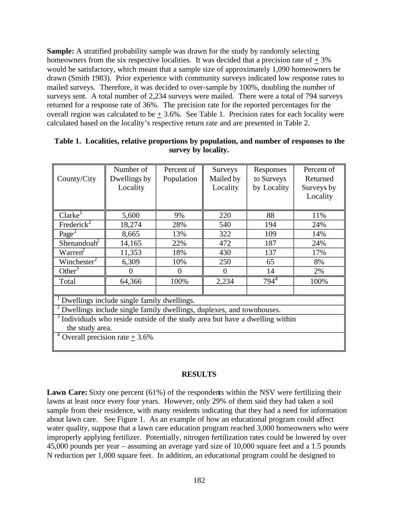
182

Sample: A stratified probability sample was drawn for the study by randomly selecting homeowners from the six respective localities. It was decided that a precision rate of + 3% would be satisfactory, which meant that a sample size of approximately 1,090 homeowners be drawn (Smith 1983). Prior experience with community surveys indicated low response rates to mailed surveys. Therefore, it was decided to over-sample by 100%, doubling the number of surveys sent. A total number of 2,234 surveys were mailed. There were a total of 794 surveys returned for a response rate of 36%. The precision rate for the reported percentages for the overall region was calculated to be + 3.6%. See Table 1. Precision rates for each locality were calculated based on the locality’s respective return rate and are presented in Table 2.

Table 1. Localities, relative proportions by population, and number of responses to the

survey by locality.

County/City

Number of Dwellings by

Locality

Percent of Population

Surveys Mailed by Locality

Responses to Surveys by Locality

Percent of Returned

Surveys by Locality

Clarke1 5,600 9% 220 88 11% Frederick2 18,274 28% 540 194 24% Page2 8,665 13% 322 109 14% Shenandoah2 14,165 22% 472 187 24% Warren2 11,353 18% 430 137 17% Winchester2 6,309 10% 250 65 8% Other3 0 0 0 14 2% Total 64,366 100% 2,234 7944 100% 1 Dwellings include single family dwellings. 2 Dwellings include single family dwellings, duplexes, and townhouses. 3 Individuals who reside outside of the study area but have a dwelling within the study area. 4 Overall precision rate + 3.6%

RESULTS Lawn Care: Sixty one percent (61%) of the respondents within the NSV were fertilizing their lawns at least once every four years. However, only 29% of them said they had taken a soil sample from their residence, with many residents indicating that they had a need for information about lawn care. See Figure 1. As an example of how an educational program could affect water quality, suppose that a lawn care education program reached 3,000 homeowners who were improperly applying fertilizer. Potentially, nitrogen fertilization rates could be lowered by over 45,000 pounds per year – assuming an average yard size of 10,000 square feet and a 1.5 pounds N reduction per 1,000 square feet. In addition, an educational program could be designed to

183

quantify reductions in nitrogen and phosphorus fertilizer use, as well as in improving fertilizer application techniques. See Table 2 for lawn care practices by locality. Pesticide Use: Almost one-half (43%) of the residents in the sample said they had used a weed killer on their lawns within the past two years. See Figure 1. Of these, over one-half said that they would like to have more information about lawn care that includes recommended practices associated with using a pesticide. See Table 2 for pesticide use by locality.

Figure 1. Lawn Care Practices

0%

20%

40%

60%

80%

100%

Homes wLawns

Homes thatfertilize lawns

Home thatfertilize &soil test

Homes thatuse weed

killer

Homes thatuse a lawn

care service

Vegetable Gardens: About one-third (38%) of the respondents said that they had a vegetable garden. About one-fourth of these said they had conducted a soil test. See Figure 2. From 1998 through June 2002, the Virginia Tech Soil Testing Laboratory analyzed 353 soil samples from vegetable gardens within the NSV. Fifty-eight percent (58%) of the samples exceeded the recommended 55-PPM mechlich 1 P. See Table 2 for vegetable garden practices by locality.

Figure 2. Vegtable Garden Practices

0%

20%

40%

60%

80%

100%

Homes w vegtable garden Homes w vegtable garden & soiltest

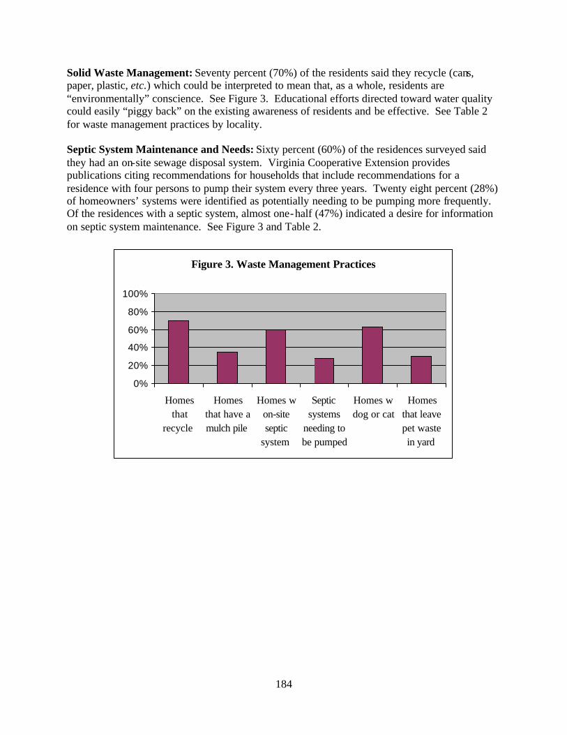
184

Solid Waste Management: Seventy percent (70%) of the residents said they recycle (cans, paper, plastic, etc.) which could be interpreted to mean that, as a whole, residents are “environmentally” conscience. See Figure 3. Educational efforts directed toward water quality could easily “piggy back” on the existing awareness of residents and be effective. See Table 2 for waste management practices by locality. Septic System Maintenance and Needs: Sixty percent (60%) of the residences surveyed said they had an on-site sewage disposal system. Virginia Cooperative Extension provides publications citing recommendations for households that include recommendations for a residence with four persons to pump their system every three years. Twenty eight percent (28%) of homeowners’ systems were identified as potentially needing to be pumping more frequently. Of the residences with a septic system, almost one-half (47%) indicated a desire for information on septic system maintenance. See Figure 3 and Table 2.

Figure 3. Waste Management Practices

0%

20%

40%

60%

80%

100%

Homesthat

recycle

Homesthat have amulch pile

Homes won-siteseptic

system

Septicsystems

needing tobe pumped

Homes wdog or cat

Homesthat leavepet wastein yard

185

Table 2. Residential practices by region effecting water quality.

Total Clarke Fredrick Page Shen. Warren Winchester

Precision + 3.6%

+ 11%

+ 7%

+ 10%

+ 7%

+ 9%

+ 12%

Lawn Care

Homes with lawns 95% 756

95% 84

96% 186

95% 104

94% 175

95% 130

100% 65

Homes that fertilize their lawns

61% 484

52% 46

70% 135

53% 58

59% 111

57% 78

72% 47

Homes that fertilize their lawns & have soil tested

29% 138

52% 24

25% 34

24% 14

23% 25

26% 20

38% 18

Homes that use weed killer on their lawns

43% 343

33% 29

46% 89

37% 40

39% 73

42% 57

74% 48

Homes that use a lawn care service

8% 63

3% 3

9% 18

3% 3

7% 13

4% 6

26% 17

Vegetable Garden

Homes that have a vegetable garden

38% 298

43% 38

32% 63

38% 41

53% 100

28% 38

22% 14

Homes that have a vegetable garden & have soil tested

26% 77

34% 13

19% 12

20% 8

37% 37

11% 4

7% 1

Waste Management

Homes that recycle 70% 558

72% 63

64% 124

54% 59

74% 138

74% 102

94% 61

Homes having a mulch pile

35% 281

52% 46

39% 75

23% 25

34% 63

35% 48

28% 18

Homes with an on-site septic system

60% 480

80% 70

54% 104

64% 70

74% 138

64% 87

6% 4

Homes having a dog or cat

63% 501

76% 67

66% 129

65% 71

53% 99

67% 92

57% 37

Homes that leave pet waste in the yard

30% 237

43% 38

28% 54

32% 35

27% 50

34% 46

17% 11

186

DISCUSSION AND IMPLICATIONS

The homeowners responding to the needs assessment reported several behaviors relating to water quality. These behaviors include: 1) not taking soil samples of their lawns and gardens; 2) probable improper use of weed killers; 3) recycling cans, paper, and plastic; and 4) for homeowners using septic systems, potentially needing to pump their systems. In addition, respondents were using large, and often unnecessary, amounts of pesticides on their lawns and vegetable gardens. The homeowners reported a willingness to learn more about what they might do to improve water quality within the region, specifically wanting information on the proper use of weed killers and wanting information on onsite system maintenance. A consistent and positive finding from the assessment was that the residents wanted more information regarding practices influencing water quality. Conclusions drawn from the collected assessment information include an increase in water quality within the region by altering behavior(s) that affect water quality. Such behavioral changes (which could be proceeded by awareness changes, and/or knowledge and/or skill changes) related to protecting water quality could be accomplished through properly directed and constructed educational programs.

REFERENCES

Aveni, M., K. Carter, S. Craik, W. Kerns, R. Prunty, and D. Relf. 2001. The Chesapeake Bay Residential Watershed Water Quality Management Program: Reducing Non-Point Source Pollution through Proper Lawn Care Practices. Virginia Cooperative Extension. Blacksburg, Va. (Publication 448-113). Chalmers, D. 2001. Personal Communication. Turfgrass Specialist, Virginia Cooperative Extension, Department of Crop and Soil Environmental Sciences. Blacksburg, Va. Smith, M. F. (Editor). 1983, October. Sampling Considerations in Evaluating Cooperative Extension Programs. (Available from Florida Cooperative Extension Service).

187

LOCAL REGULATION TO PROTECT SOURCE WATER IN KARST TERRAIN IN VIRGINIA

Jesse J. Richardson, Jr.

Department of Urban Affairs and Planning Virginia Tech

Blacksburg, VA 24061-0113 jessej@vt.edu

KEY WORDS: karst, land use, source water protection, ordinances

INTRODUCTION This paper focuses on local regulation of land use to protect groundwater quality in Virginia. Specifically, the analysis centers on the results of a survey of local governments within the karst belt of Virginia and West Virginia. This survey, sponsored by the Cave Conservancy of the Virginias and conducted by the author, sought to ascertain the existence of specific karst provisions in planning and regulatory documents in these two states. This paper emphasizes the results from Virginia pertaining to source water protection. The survey results suggest that local governments in Virginia fail to adequately protect groundwater quality and quantity through land use regulation. The conclusion provides suggestions for higher levels of protection.

METHODS

During late 2002 and early 2003, the author, operating with a grant from the Cave Conservancy of the Virginias, surveyed the seventy-four local governments within Virginia and West Virginia whose boundaries include karst terrain. The survey included fifty-four localities in Virginia and twenty localities in West Virginia. The Virginia localities consist of twenty-eight counties, thirteen cities, and thirteen towns (towns with populations over 2,000 were included). The survey targeted local land use planners where possible, with the local government administrator or governing body serving as default contacts. The survey sought to discover the level of familiarity with karst among local government planners, the level of concern by local government planners and officials with respect to specific karst issues, and the number of local governments specifically addressing karst within their planning and regulatory provisions. The principal investigator first mailed the survey to the contact persons in each locality. After approximately three weeks, non-responding localities were contacted by telephone or electronic mail.

188

RESULTS This summary focuses exclusively on the responses from Virginia localities. Fifty local governments in Virginia responded to the survey (93% of those surveyed). Government officials in all responding Virginia localities expressed familiarity with karst. Approximately twenty-two percent of the Virginia local government officials regarded themselves and/or their staffs as “very familiar” with the implications of karst, while thirty-one percent, identified themselves as “familiar,” and thirty-nine percent considered themselves as “somewhat familiar” with the concept.* Local government officials expressed relatively high levels of concern for surface water contamination, groundwater contamination, and adequate supplies of surface and groundwater. The author speculates that respondents registered elevated concerns for water supplies due to the prolonged and ongoing drought. Respondents failed to hold significant concerns in other areas. Stormwater management issues appeared particularly insignificant to respondents. Twenty-six responding local governments, or fifty- two percent, include karst provisions in their comprehensive plan. Characteristically, the comprehensive plan provisions contain general, aspirational statements. Highland County’s plan proves typical. The plan first describes karst and sinkholes and delineates the hazards of developing in karst areas. The plan declares that “In order to reduce the risk of damage from subsidence or collapse in karst terrain, development on existing sinkholes should be avoided completely. All potential development in Highland County should be proceeded by test borings to determine whether or not hidden cavernous zones are present” (Highland County, Virginia Comprehensive Plan (undated)). The karst section of the plan also includes concerns about groundwater contamination (Ibid). Other plans, like the Shenandoah County, Virginia Comprehensive Plan (draft) focus exclusively upon groundwater contamination issues. A much smaller number of Virginia localities actually implement the provisions within the comprehensive plan. Six Virginia localities implement those provisions within the zoning ordinance, and seven include karst-specific subdivision provisions. A handful of local governments in Virginia maintain karst-related ordinances relating to stormwater (4), waste management (3), water supply protection (3) or community household hazardous waste or agricultural waste (2). Of the localities adopting zoning or subdivision ordinances to address karst issues, all nine include karst concerns within the comprehensive plan. Four local governments additionally address karst with both zoning and subdivision provisions. Only the zoning ordinance provision furthers the karst goals of the comprehensive plan in two localities, while three local governments use only subdivision ordinance provisions to advance karst goal. * The survey defined “very familiar” as having staff members who had attended more than 2 conferences or workgroup meetings pertaining to karst within the last three years. A designation of “familiar” denoted recognition of karst as an important land use planning issue, along with a conscious effort to educate staff on karst. “Somewhat familiar” referred to those staffs with knowledge of karst and the ability to identify features but failed to recognize the significance of karst in land use planning (Karst Protection Survey 2002).

189

Of the six Virginia zoning ordinances that reportedly reference karst issues, only two of these provisions address the concerns in a meaningful fashion. Clarke County uses separate provisions in the zoning ordinance, septic ordinance, the water well ordinance, and a sinkhole ordinance to regulate development in karst areas within the county. The zoning ordinance employs a spring conservation overlay district to prohibit certain uses, prescribe minimum lot sizes and regulate subsurface septic systems in karst areas. A separate zoning provision sets forth stricter requirements for land application of biosolids on karst than otherwise allowed. Clarke’s sinkhole ordinance distinguishes between Class 1 and Class 2 sinkholes. Class 1 sinkholes present significant subsurface water pollution hazard if, due to drainage patterns of the land surrounding the sinkhole or the nature of the substances or objects in the sinkhole, the sinkhole may permit the entry of pollutants into subsurface water. All other sinkholes fall under Class 2. Class 1 sinkholes must be identified; and the county may prescribe corrective and protective measures, including vegetated buffer zones, installation of diversion methods or structures, concrete or plastic liners, termination of pollution hazard activity, and removal of substances and objects from the sinkhole. Loudoun County adopted the Limestone Overlay District in January 2003. These regulations apply to all land disturbing activity within the limestone area of the county, with few exceptions. A landowner must obtain a geotechnical or geophysical study and must identify sinkholes, closed depressions, outcrops, surface drainage to ground, and other features prior to the activity. The provisions also include required buffer areas around all karst features, including a fifty-foot buffer area measured from any limestone outcrop and a one hundred-foot buffer area around any sinkhole rim. In addition, the rules prohibit subdivisions of eight or more lots except with special exception and prohibit structures in subsidence areas. Site grading may not affect surface flow into sinkholes or springs. The county may require mitigation measures such as nutrient management plans, clustering of structures, or reductions in impervious services. Finally, the provisions require a warning to property owners on the subdivision plat with respect to application of fertilizers, pesticides, and similar substances. Seven localities in Virginia address karst issues within their subdivision ordinance. Most, however, use broad vague provisions that are likely unenforceable if challenged. The decision of whether to grant a subdivision request amounts to an administrative decision, as opposed to the legislative nature of rezoning requests. Therefore, subdivision ordinances must contain specific guidelines and leave little discretion to the administrator. Giles County’s subdivision ordinance typifies the vague, general nature of karst subdivision ordinances in Virginia. The ordinance proclaims that, “[l]and subject to flooding and land deemed to be topographically unsuitable (for reasons such as unstable slopes, the presence of sinkholes, caves and interior drainage) shall not be platted for residential occupancy, nor for such other uses as may increase the danger of health, life or property, or aggravate erosion or flood hazard….” (Giles County Subdivision Ordinance (undated). This provision gives the local subdivision administrator too much discretion in deciding the scope of “land topographically unsuitable.”

190

DISCUSSION

Development in communities characterized by karst terrain often raises the possibility of flooding, surface and groundwater contamination, and subsidence. Response to these hazards incurs substantial costs for the public and private sector. These costs can be greatly reduced through a proactive program to address potential hazards before intensive development occurs. Few Virginia local governments within the karst belt presently take substantive action within land-use planning and regulation to address karst issues. However, a substantial number of Virginia local governments include karst considerations within their comprehensive plans. The raising of the issues in the comprehensive plans takes the first step forward in planning for the effects of development in karst. In many localities, planners and government officials must incrementally approach regulation of karst impacts, and comprehensive plan provisions lay the framework for future action. Present regulations and model ordinances across the country provide guidance for localities in Virginia and other states to proactively address land use impacts of development in karst before these issues become problems. The major lessons learned from other jurisdictions focus on the need for data collection and education of planners, government officials and the general public as the first steps toward effective regulation of development in karst terrain.

ACKNOWLEDGMENTS

The research for this article was made possible by a grant from the Cave Conservancy of the Virginias and funding from the Department of Urban and Affairs and Planning at Virginia Tech, Blacksburg, Virginia. The author acknowledges the research and hard work put forth by Brad Belo, graduate research assistant.

REFERENCES Clarke County, Va. (undated). Sinkhole Ordinance (Chap. 180: Water and Wastewater – Article 2). Giles County, Va. (undated). Subdivision Ordinance. Highland County, Va. (undated). Comprehensive Plan. Loudoun County, Va. (2003). Limestone Conglomerate Overlay District (LCOD). Shenandoah County, Va. (draft). Virginia Comprehensive Plan.

191

EFFECTS OF AGRICULTURAL DISTURBANCE ON AUTUMN ALLOCHTHONOUS INPUT TO SOUTHERN APPALACHIAN STREAMS

Elizabeth M. Hagen and Jackson R. Webster

Department of Biology, Virginia Tech Blacksburg, VA 24061

ehagen@vt.edu

KEY WORDS: agriculture, allochthonous input, land use, leaf litter

ABSTRACT Anthropogenic changes in catchment use, such as agriculture, can result in disturbances to freshwater ecosystems. The purpose of this study was to assess the impact of agricultural land use on autumn allochthonous input to southern Appalachian streams. Allochthonous input was measured in twelve streams with differing degrees of agricultural land use. Input ranged from 4 to 343 g AFDM m-2, with higher values recorded in forested and light agricultural streams. Allochthonous input peaked in November in forested streams, but was highest in September and November in agricultural streams.

INTRODUCTION Streams and adjacent riparian vegetation are linked through allochthonous organic matter inputs from terrestrial ecosystems. In forested streams, over 90% of the streams energy may come from allochthonous input (Fisher and Likens 1973). Allochthonous inputs consist of material entering streams from riparian vegetation, including leaves, floral parts, wood, cones, nuts, and fruits (Benfield 1997). Leaves usually make up the largest component of allochthonous input, ranging anywhere from 41% to 98% of total input (Abelho 2001). Agricultural land use can result in persistent disturbance to freshwater ecosystems (Harding et al. 1998). These disturbances often include a reduction of riparian vegetation. The riparian zone is an important buffer between the stream and its surrounding land use. Additionally, the riparian zone can be the primary source of organic matter to small, forested streams. It can improve water quality, reduce sedimentation, and control temperature regimes (Harding et al. 1998). The objective of this study was to measure the impact of agricultural disturbance on the quantity, composition, and seasonal distribution of allochthonous organic matter input to southern Appalachian streams.

METHODS

Allochthonous input was measured from September through December 2002 in twelve streams with four degrees of land use: forest and light, moderate, and heavy agriculture. Streams were characterized based on land use adjacent to the stream (Table 1). Forested streams have an intact riparian zone and no agricultural land use present in its watershed. Light agricultural streams have areas of pasture close to the stream, but the riparian vegetation is intact and the watershed

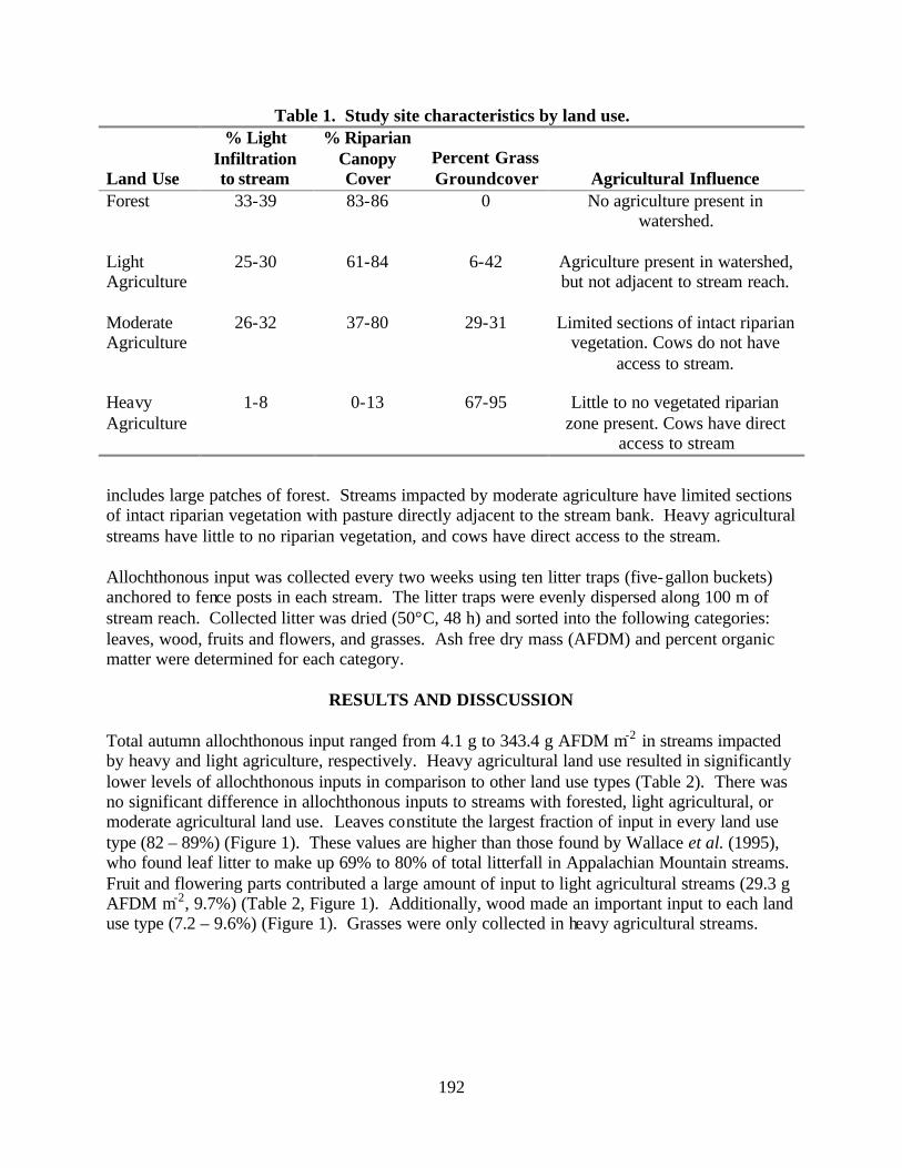
192

Table 1. Study site characteristics by land use.

Land Use

% Light Infiltration to stream

% Riparian Canopy Cover

Percent Grass Groundcover Agricultural Influence

Forest 33-39 83-86 0 No agriculture present in watershed.

Light Agriculture

25-30

61-84 6-42 Agriculture present in watershed, but not adjacent to stream reach.

Moderate Agriculture

26-32 37-80 29-31 Limited sections of intact riparian vegetation. Cows do not have

access to stream.

Heavy Agriculture

1-8 0-13 67-95 Little to no vegetated riparian zone present. Cows have direct

access to stream

includes large patches of forest. Streams impacted by moderate agriculture have limited sections of intact riparian vegetation with pasture directly adjacent to the stream bank. Heavy agricultural streams have little to no riparian vegetation, and cows have direct access to the stream. Allochthonous input was collected every two weeks using ten litter traps (five-gallon buckets) anchored to fence posts in each stream. The litter traps were evenly dispersed along 100 m of stream reach. Collected litter was dried (50°C, 48 h) and sorted into the following categories: leaves, wood, fruits and flowers, and grasses. Ash free dry mass (AFDM) and percent organic matter were determined for each category.

RESULTS AND DISSCUSSION

Total autumn allochthonous input ranged from 4.1 g to 343.4 g AFDM m-2 in streams impacted by heavy and light agriculture, respectively. Heavy agricultural land use resulted in significantly lower levels of allochthonous inputs in comparison to other land use types (Table 2). There was no significant difference in allochthonous inputs to streams with forested, light agricultural, or moderate agricultural land use. Leaves constitute the largest fraction of input in every land use type (82 – 89%) (Figure 1). These values are higher than those found by Wallace et al. (1995), who found leaf litter to make up 69% to 80% of total litterfall in Appalachian Mountain streams. Fruit and flowering parts contributed a large amount of input to light agricultural streams (29.3 g AFDM m-2, 9.7%) (Table 2, Figure 1). Additionally, wood made an important input to each land use type (7.2 – 9.6%) (Figure 1). Grasses were only collected in heavy agricultural streams.

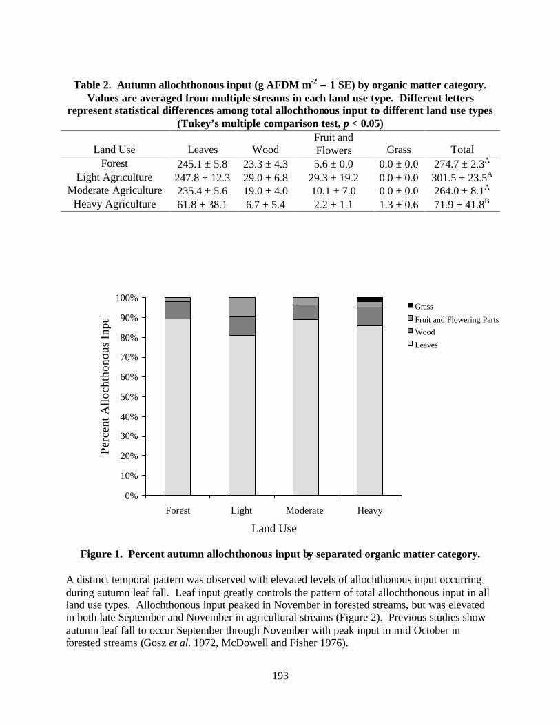
193

Table 2. Autumn allochthonous input (g AFDM m-2 ± 1 SE) by organic matter category.

Values are averaged from multiple streams in each land use type. Different letters represent statistical differences among total allochthonous input to different land use types

(Tukey’s multiple comparison test, p < 0.05)

Land Use Leaves Wood Fruit and Flowers Grass Total

Forest 245.1 ± 5.8 23.3 ± 4.3 5.6 ± 0.0 0.0 ± 0.0 274.7 ± 2.3A Light Agriculture 247.8 ± 12.3 29.0 ± 6.8 29.3 ± 19.2 0.0 ± 0.0 301.5 ± 23.5A

Moderate Agriculture 235.4 ± 5.6 19.0 ± 4.0 10.1 ± 7.0 0.0 ± 0.0 264.0 ± 8.1A Heavy Agriculture 61.8 ± 38.1 6.7 ± 5.4 2.2 ± 1.1 1.3 ± 0.6 71.9 ± 41.8B

0%

10%

20%

30%

40%

50%

60%

70%

80%

90%

100%

Forest Light Moderate Heavy

Land Use

Grass

Fruit and Flowering PartsWood

Leaves

Perc

ent A

lloch

thon

ous

Inpu

t

Figure 1. Percent autumn allochthonous input by separated organic matter category. A distinct temporal pattern was observed with elevated levels of allochthonous input occurring during autumn leaf fall. Leaf input greatly controls the pattern of total allochthonous input in all land use types. Allochthonous input peaked in November in forested streams, but was elevated in both late September and November in agricultural streams (Figure 2). Previous studies show autumn leaf fall to occur September through November with peak input in mid October in forested streams (Gosz et al. 1972, McDowell and Fisher 1976).

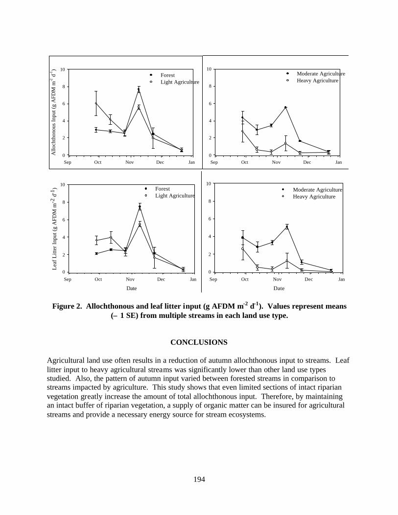
194

Sep Oct Nov Dec Jan

Allo

chth

onou

s In

put (

g A

FDM

m-2

d-1

)

0

2

4

6

8

10ForestLight Agriculture

Sep Oct Nov Dec Jan 0

2

4

6

8

10Moderate AgricultureHeavy Agriculture

Date

Sep Oct Nov Dec Jan

Lea

f Litt

er In

put (

g A

FDM

m-2

d-1

)

0

2

4

6

8

10ForestLight Agriculture

Date

Sep Oct Nov Dec Jan 0

2

4

6

8

10Moderate AgricultureHeavy Agriculture

Figure 2. Allochthonous and leaf litter input (g AFDM m-2 d-1). Values represent means (± 1 SE) from multiple streams in each land use type.

CONCLUSIONS Agricultural land use often results in a reduction of autumn allochthonous input to streams. Leaf litter input to heavy agricultural streams was significantly lower than other land use types studied. Also, the pattern of autumn input varied between forested streams in comparison to streams impacted by agriculture. This study shows that even limited sections of intact riparian vegetation greatly increase the amount of total allochthonous input. Therefore, by maintaining an intact buffer of riparian vegetation, a supply of organic matter can be insured for agricultural streams and provide a necessary energy source for stream ecosystems.

195

ACKNOWLEDGMENTS We would like to thank Matthew Beversdorf, Holly Houtz, Robert Payn, Virginia Presley, and Olyssa Starry for assistance in the field and the Virginia Tech Stream Team for constructive comments.

REFERENCES

Abelho, M. 2001. From litterfall to breakdown in streams: A review. The Scientific World 1: 1-25. Benfield, E. F. 1997. Comparison of litterfall input to streams. Journal of the North American Benthological Society 16(1): 104-108. Fisher, S. G. and G. E. Likens. 1973. Energy flow in Bear Brook, New Hampshire: An integrative approach to stream ecosystem metabolism. Ecological Monographs 43: 421-439. Gosz, J. R., G. E. Likens, and F. H. Bormann. 1972. Nutrient content of litter fall on the Hubbard Brook Experimental Forest, New Hampshire. Ecology 53(5): 769-784. Harding, J. S., E. F. Benfield, P. V. Bolstad, G. S. Helfman, and E. B. D. Jones III. 1998. Stream biodiversity: The ghost of land use past. Proc. Natl. Acad. Sci. 95: 14843-14847. McDowell, W.H. and S. G. Fisher. 1976. Autumnal processing of dissolved organic matter in a small woodland stream ecosystem. Ecology 57: 561-569. Wallace, J. B., M. R. Whiles, S. Eggert, T. F. Cuffney, G. J. Lughaart, K. Chung. 1995. Long-term dynamics of coarse particulate organic matter in three Appalachian Mountain streams. Journal of the North American Benthological Society 14: 217-232.

196

LOGGING, FLOODING, AND LAWSUITS: A NEW ROLE FOR BEST MANAGEMENT PRACTICES?

Michael J. Mortimer and Rien J.M. Visser

Department of Forestry, Virginia Tech Blacksburg, VA 24061

mortimer@vt.edu

KEY WORDS: timber, flooding, logging, lawsuits, best management practices

INTRODUCTION

Timber harvesting, particularly in steep upland regions, shares a controversial relationship with natural calamities, such as floods and landslides that threaten the lives and property of adjacent landowners. That relationship may manifest itself in legal proceedings, not primarily to prevent timber harvesting, but instead to seek recovery from the timber harvester for damages sustained by victims of these associated natural calamities. In July 2001, a series of large rainstorm events caused serious flooding to occur across large areas of southwest Virginia, eastern Kentucky and southern West Virginia. Over 6.5 inches of rainfall were recorded in West Virginia on July 8th, which falling on already saturated soils, caused widespread flooding. Subsequently, lawsuits were filed in several West Virginia counties by hundreds of landowners against an array of timber, coal, and mining companies. The individuals bringing the lawsuits (plaintiffs) stated that timber, coal, and mining companies (defendants) had contributed to, and were thus liable for, the property and personal damages sustained following the flooding. The plaintiffs alleged that a combination of sedimentation of the natural watercourse and increases in surface flow attributable to land management activities caused or exacerbated the flooding. Common to the lawsuits were allegations that timber harvesting was an “ultra-hazardous activity,” that timber harvesters had violated the law by not complying with West Virginia’s Best Management Practices (BMPs), and that logging had knowingly altered the natural stream flows by accelerating water runoff. Many of the legal allegations, however, are not well grounded in science. The most reliable research information with regard to a possible increase in peak flood flow comes from long-term paired watershed studies. Examples of these include those carried out by the Forest Service at Coweeta, North Carolina (Swank and Crossley 1988), the Fernow Experimental Forest in West Virginia (Kochenderfer et al. 1990) and at Hubbard Brooks Experimental Forest in New Hampshire (Hornbeck et al. 1997). While all studies concur that clear-cutting the whole watershed increases base-flow for a period of two to five years (Aust and Blinn 2003), actual increases in flood flow response, although real, have a weaker relationship (e.g., Hornbeck 1973, Patrick 1980, Miller 1984, Hornbeck and Kochenderfer 2000). This led most studies to conclude that increases in peak flows typically are limited to the first few growing seasons. Opinions expressed in this paper are those of the authors and not of the Virginia Water Resources Research Center.

197

The actual magnitude of any peak flow is very dependant on other factors, e.g., was the soil already saturated from previous rainfalls or did the storm move up or down the watershed? In the five years after clear-cutting at the Fernow Experimental Forest, 16 flood flows were measured, and only five were significantly higher in the clear-cut watershed. The increase for these five events ranged from 9% to 69% (Kochenderfer and Hornbeck 1999). When considering the inability to accurately model a flood event retrospectively given the entire storm and soil moisture condition information, we conclude that neither probability nor magnitude of increase is predictable. Nonetheless, legal attempts to link timber harvesting with flood events suggest that the time is ripe to consider a new category of BMPs, one that addresses the rate and volume at which water is produced in a watershed. The most pragmatic approach to dealing with flood risk associated with timber harvesting is to identify and ratify water quantity BMPs. This approach includes (a) identifying those water quality BMPs that also meet water quantity goals (e.g., waterbars, cut-outs, revegetation requirements), (b) providing some balance to those BMPs where water quality and quantity would be contradictory (e.g., culverts, ditches), (c) recognizing the benefit of and modifying BMPs driven by other motives such as visual or wildlife habitat, and finally (d) introducing new water quantity BMPs. An example of a BMP driven by wildlife and visual impact consideration is the clear-cut limits set out by the Sustainable Forestry Initiative or the Forest Stewardship Council. Introducing a variable that considers what percentage of the watershed will be harvested could help mitigate potential flow increases. An example for a new water quantity BMP could be the ripping of designated skid trails to improve water penetration and dispersion – albeit at the risk of increased erosion. A comprehensive review of southeastern studies indicates that current BMPs are very effective at mitigating harvesting impacts with regard to water quality, base flow, and site productivity (Aust and Blinn 2003). Most researchers also conclude that increases in peak flood-flows are short in duration and typically insignificant at the larger watershed level. However, there are a number of issues relating to BMPs open to discussion, including (a) proving compliance with the current BMP standards, (b) the spatial scale at which to consider peak-flow impacts and the accumulative impact of other land users that share a watershed, and (c) the liability for structures in a recognized flood zone downstream. (a) BMP compliance is neither simple nor exact, with many aspects open to interpretation. Most Departments of Forestry, therefore, encourage interaction and discussion with local officials to establish “compliance standards.” Self-auditing is an accepted method for avoiding complications with BMP compliance as well as providing for ongoing improvement. However, these internal audits may be subpoenaed by a court of law, and the question arises, “If a lack of a certain BMP is identified by the forester and is cited to be rectified, does this admit non-compliance for the period between the activity and rectification?” This question is primarily a temporal one, and time frames for BMP implementation are rarely set. Secondly, in southeastern states the respective Departments of Forestry audit either a sample or all harvested sites once they are closed. Does a successful compliance audit by the state indemnify that site? (b) The spatial scale at which to consider land management activities is another issue rarely addressed. Typical harvest operations range from approximately 10-150 acres. At a larger

198

watershed scale (25,000 acres or more), timber harvesting will rarely modify more than 2% of the overall watershed. Also, once a harvest site revegetates, typically between two to five years in the Appalachian area (Aust and Blinn 2003), the hydrological responses to storm events are not significantly different than that of a mature forest (Kochenderfer and Hornbeck 1999). The second related component to this issue of spatial scale is the relative impact of other land uses. With regard to peak flood-flow response, it is possible to relatively rank different land uses. Commercial areas, urban areas, developed areas including residential housing, and road infrastructure creates the largest increase in flood flow, followed by agriculture and finally forested land under management. When determining impacts one could easily argue that the relative impact would need to be quantified relative to the different land uses in the watershed. However, two spatial factors complicate this accumulative impact evaluation. First, timber harvesting is the activity commonly higher up in the watershed, therefore impacting downstream land users. For example, urban- induced increases in flooding rarely impact forestry except in coastal areas. Secondly, timber harvesting is an activity typically on steeper slopes, and steep slopes naturally have a faster hydrological response to a given rainfall event. (c) Most flood damage occurs in the flood zone surrounding the streams and rivers. Bridges and roads built to withs tand a 100-year flood can be expected to be damaged in a 100-year rainfall event. So assuming it is shown that a given land management activity is partially responsible for increasing peak flood-flow, to what extent should this affect those impacted that actually live in the flood zone? In other words, what is the share of responsibility of those who choose to reside in flood plains? In considering the legal risks, it is prudent to consider potential operational solutions, including clarifying the role that forestry BMPs play. While some states have comprehensive Forest Practice Acts that avoid the ambiguity of voluntary BMPs, studies have shown that BMPs are a more cost effective way of managing and improving environmental performance compared to the regulatory approach (Aust and Shaffer 1996). A fundamental question would be, should implementation and compliance with BMPs, in whatever form they may take, insulate a logging operation from various legal claims? For example, while only two southern states currently have mandatory BMPs, most of the remaining nonregulatory states reflect linkages between BMPs and water quality laws, or in some other manner assess the application or implementation of BMPs. These linkages to other legal requirements or to quasi-regulatory performance standards may have legal ramifications. Imagine a court tasked with determining whether a logger in a flooding case violated the “law.” What would the court review? The water quality law itself, the BMPs related to the law and designed to implement it, the extent to which BMPs were complied, or some amalgam of all of these? The intriguing and frightening problem is that even in nonregulatory states, BMPs nonetheless play a quasi-regulatory role, providing performance standards that afford the opportunity for court challenges unrelated to scientific and operational realities. Unfortunately, the West Virginia litigation raises far more questions than it answers. And any answers will likely be years in the making. It does, however, provide impetus to appraise the

199

current use of best management practices, and the potentially antagonistic relationship between mitigating water quantity and quality in flood-prone regions. If the plaintiffs in the West Virginia litigation succeed, timber harvesting in mountainous terrain, and the role of forestry BMPs may both be faced with challenging precedent.

REFERENCES Aust, W.M and R.M. Shaffer. 1996. Benefits and costs of forestry best management practices in Virginia. Southern J. Appl. Res. 20(1): 23-29. Aust, W.M and C.R. Blinn. In press. Forestry best management practices for timber harvesting and site preparation in the eastern United States: An overview of water quality and productivity research during the past 20 years 1982-2002. Accepted by Water, Air, and Soil Pollution Focus. 29 pp. Hornbeck, J.W. 1973. Storm flow from hardwood-forested and cleared watersheds in New Hampshire. Water Resoures Res. 9(2): 346-354. Hornbeck, J.W. and J.N. Kochenderfer. 2000. Linkages between forests and streams: A perspective in time. In: Riparian Management in Forests of the Continental Eastern United States. E.S. Verry, J.W. Hornbeck, and C.A. Doloff (Editors). Lewis Publishers. Washington D.C. pp 89-97. Hornbeck, J.W., C.W. Martin, and C. Edgar. 1997. Summary of water yield experiments at Hubbard Brook Experimental Forest, New Hampshire. Canadian J. Forest Res. 27: 2043-2052. Kochenderfer, J.N., J.D. Helvey, J.H. Patrick, and W.E. Kidd. 1990. Woodlot Management: An Introduction to Water in the Forest. USDA Forest Service, Northeastern Forest Experiment Station, Timber and Watershed Laboratory. Parsons, W.Va. 28 pp. Kochenderfer, J.N. and J.W. Hornbeck. 1999. Contrasting timber harvest operations illustrate the value of BMPs. In: Proceedings, 12th Central Hardwoods Forest Conference; Feb. 1999, 28 March; Lexington, K.Y. J.W. Stringer and D.L. Loftis (Editors). Gen. Tech. Rep. USDA Forestry Service, Southern Research Station. Ashville, N.C. Miller, E.L. 1984. Sediment yield and storm flow response to clear-cut harvest and site preparation in the Ouachita Mountains. Water Resources Res. 20(4): 471-475. Patrick, J.H. 1980. Effects of wood products harvest on soil and water relations. J. Env. Qual. 9(1): 73-80. Swank, W.T. and D.A. Crossley (Editors). 1988. Forest Hydrology and Ecology at Coweeta. Ecol. Studies 66. Springer-Verlag. New York, N.Y. 469 pp.