water quality analysis report - ssrws
TRANSCRIPT

1 of 106 Giesy et al, April 7, 2009
WATER QUALITY ANALYSIS REPORT
Nutrient loading and toxic algal blooms in Lake Diefenbaker
Report to: Mr. James, Tucker General Manager
Mid Saskatchewan Regional Economic and Co-operative Development
420 Saskatchewan Ave. West, P.O. Box 176
Outlook, SK Canada S0L 2N0
Prepared by: John P. Giesy, Ph.D. Suqing Li, Ph.D,
and Jong Seong Khim, Ph.D
Toxicology Centre University of Saskatchewan
44 Campus Drive Saskatoon, SK S7N 5B3
March 31, 2009

2 of 106 Giesy et al, April 7, 2009
TABLE OF CONTENTS
1. INTRODUCTION……………………………………………………………………3 2. METHODS……………………………………………………………………………5
2.1 Sampling and Field Measurements……………………………………………5 2.1.1 Sample Sites………………………………………………………………5 2.1.2 Sample Collection…………………………………………………………5
2.2 Laboratory Analysis……………………………………………………………12 2.2.1 Chemical Analysis………………………………………………………12 2.2.2.Bioassays…………………………………………………………………12
2.3 Sampling and Lab Chemical Analysis QA/QC………………………………13 2.4 Testable null hypotheses and statistic analysis……………………………14
3. RESULTS AND DISCUSSION……………………………………………………15 3.1 Water Quality Analysis in Lake Diefenbaker…………………………………15
3.1.1 Three-way ANOVA with Student-Newman-Keuls Method……………15 3.1.2 Nonparametric Analysis with Kruskal-Wallis ANOVA and Median t e s t … … … … … … … … … … … … … … … … … … … … … … … … … … … 1 7
3.2 Identification of Limiting Factors for the Blue-green Algae Growth………18 3.3 Causes of Cyanobacteria Bloom in 2007……………………………………21 3.4 Algal Biomass…………………………………………………………………24 3.5 Nutrient Addition Bioassay……………………………………………………28 3.6 Satellite Image Analyses………………………………………………………37 3.7 Concentration Balance…………………………………………………………43
4. CONCLUSIONS AND RECOMMENDATIONS…………………………………55 ACKNOWLEDGEMENTS……………………………………………………………56 REFERENCES…………………………………………………………………………57 APPENDICES…………………………………………………………………………59
A. Testable Null Hypotheses and Statistic Analysis……………………………59 B. Tables of Three-way ANOVA…………………………………………………62 C. Tables of Non-parametric analysis……………………………………………74 D. Figures of Box Plots (non-parametric analysis)………………………………89 E. ELT-SOP for Lake Diefenbaker………………………………………………104

3 of 106 Giesy et al, April 7, 2009
1. INTRODUCTION Lake Diefenbaker (51°1′53″N, 106°50′9″W) is a large multi -purpose reservoir on the South Saskatchewan River in southern Saskatchewan, Canada (Fig. 1). It was formed by the construction of Gardiner Dam and the Qu'Appelle River Dam across the South Saskatchewan and Qu'Appelle Rivers respectively. It provides water for domestic irrigation and municipal water supplies and permits the regulation of the flow of the two rivers (http://www.swa.ca/). Inflow to Lake Diefenbaker is primarily from the South Saskatchewan River which originates as the Old man, Bow, and Red Deer Rivers in the mountains of southwestern Alberta. These rivers drain much of southern Alberta which, except for the mountain regions, is mainly treeless prairie used for grain and livestock production. Approximately 75% of the drainage to Lake Diefenbaker is in Alberta (http://www.ilec.or.jp/database/nam/nam-58.html). The inflowing rivers also receive irrigation return flows and municipal and industrial effluents, which resulted in the contamination of lake sediments (Gregor and Munawar, 1989) and toxic algae blooms (Reynolds and Walsby 1975; Peter et al., 2006; Jacoby et al., 2007). A cyanobacteria (formerly known as blue-green algae) bloom occurred in August & September of 2007 (http://www.waterwolf.org/PDFs). The bloom was primarily in the southern and western portions of the reservoir (http://www.menoutdoors.com/forums/showthread.php?t=7030). There are several reasons why this bloom may have occurred. These include: 1) Temperature, since the water temperature late in the year was greater than the long-term average for that time period; 2) Nutrients, since there was a relatively large local snow pack that melted relatively rapidly in the spring of 2007, more local nutrients could have been loaded into the reservoir; 3) The spring freshet could also have added micronutrients such as iron in an available form; 4) The hydrodynamics and wind patterns on the reservoir may have resulted in local conditions that favored the development of the bloom or concentrated the bloom into particular areas and thus magnified the effect; 5) Colonization source, conditions might have existed that lead to a greater source of colonization and lesser turnover of the lake that may have lead to the local outbreak; 6) Allocthonous nutrients from either point or non-point sources upstream of the reservoir; 7) Autothanous sources of nutrients in the reservoir, such as from sediments or the fish farm. This study focused primarily on the nutrient content and nutrient limitation of algal growth in Lake Diefenbaker. The primary Nutrients investigated were nitrogen and phosphorus. The study involved collecting water samples from the lake to determine nutrient concentrations and field measurements of chemical and physical immunological parameters. In particular, information was collected to conduct a rudimentary

4 of 106 Giesy et al, April 7, 2009
1
6
4 2
3 5
7
concentration balance for nitrogen and phosphorus. Specifically, the question of relative contributions from upstream and in the vicinity of the lake is being addressed. Bioassays were conducted with the natural consortium of phytoplankton and a define blue-green alga monoculture to determine the limiting factors (nitrogen and or phosphorus) for both consortia of algae collected from the lake and for specific species of cyanobacteria, such as Anabaena sp. Satellite imagery was investigated to determine its potential to quantify the distribution of chlorophyll in Lake Diefenbaker to determine the extent of the algal blooms in space and time.
Fig. 1. Map of Lake Diefenbaker showing sampling locations (n=7)

5 of 106 Giesy et al, April 7, 2009
2. METHODS 2.1 Sampling and Field Measurements 2.1.1 Sample Sites Based on the basic information and the characteristics of topography, size, shape, depth, flow velocity, etc. 7 sampling sites in Lake Diefenbaker were selected (Table 1; Fig. 2). 2.1.2 Sample Collection Water samples were collected every month from June to October 2008 (Table 2). Sampling was conducted between 10 a.m. and 6 p.m. based on weather conditions (OECD, 1982). Except for collections at the outflow (site7), where only surface water was collected, at each sampling location, the sampling site was located by GPS and the boat was anchored to avoid drifting and 3 stratified water samples were collected according to the water depth, as follows: 1) Surface: water surface at a depth of 0.5 m. 2) Mid-depth. 3) Bottom: 0.5 m above bottom. A total of 81 samples were collected for nutrient analyses. All the parameters measured in Lake Diefenbaker are listed in Table 3-5. ETL-SOPs had been prepared for all activities proposed (Table 6). Table 1. Geographical location of sampling sites in Lake Diefenbaker.
Site Description Latitude (N)
Longitude (W)
Elevation (m)
1 Saskatchewan Landing Provincial Park 50°39'55.8'' 107°57'1.6'' 564 2 Upstream of Fish Farm 50°51'34.4'' 106°57'1.6'' 554 3 Downstream of Fish Farm 50°58'56.5'' 106°53'58.1'' 554 4 Qu’Appelle Dam 51°00'0.06'' 106°28'52.9'' 554 5 Elbow 51°06'1.02'' 106°37'0.0'' 555 6 Gardiner Dam 51°13'53.5'' 106°49'10.3'' 554 7 Hydroelectric Power Station 51°16'42.7'' 106°52'35.8'' 500

6 of 106 Giesy et al, April 7, 2009
Fig.2. Map of Lake Diefenbaker showing water depth (m) and seven (7) sampling
locations in Google Earth.

7 of 106 Giesy et al, April 7, 2009
Table 2. Dates of field sampling and laboratory analyses (April 2008 to March 2009).
Date Task Date Task Apr 15-30 Study plan Oct 3-24 Bioassay-1 May 1-15 Equipments arrangement Oct 23-24 Sampling-5 May 16-25 Sample preparation Oct 25- Dec 2 Lab analysis May 26-28 Personnel recruit & training Dec 5-19 Bioassay-2 May 29 Field survey Dec 20-Jan 12 Lab analysis May 30-Jun 23 Sample preparation Dec 22-Jan 4 Bioassay-3 Jun 24, 29-31 Sampling-1 Jan 5-25 Lab analysis Jun 28-Jul 22 Lab analysis Jan 12-26 Bioassay-4 Jul 24, 31 Sampling-2 Jan 27- Feb 10 Lab analysis Aug 1-25 Lab analysis Feb 11-16 Data input & check Aug 26-27, 29 Sampling-3 Feb 17-21 Data analysis Sep 1-28 Lab analysis Feb 22- Mar 15 Research report Sep 29-30 Sampling-4 Mar 16-28 Manuscript prep. Oct 1-22 Lab analysis Mar 29-30 Manuscript sub.

8 of 106 Giesy et al, April 7, 2009
Table 3. Water quality parameters measured in Lake Diefenbaker.
Parameter Unit Methodology Instrument References In Situ Measurements Water temperature oC Hydrolab DS5 pH pH units Electrometric Hydrolab DS5 Electrical conductance (EC)
us/cm Conductivitymetric Hydrolab DS5
Turbidity ntu Nephelometric Hydrolab DS5 Dissolved oxygen (DO)
mg/l Dissolved Oxygen Metric
Hydrolab DS5
Chlorophyll a (Chla) µg/l Colorimetric Hydrolab DS5 Salinity ppt Hydrolab DS5 Total Dissolved Solids (TDS)
g/l Hydrolab DS5
Depth m Hydrolab DS5 Laboratory Measurements Hardness (as CaCO3)
mg/l Titration, using EDTA Titrator Hach 8213
Alkalinity (as CaCO3)
mg/l Phenolphthalein Digital Titration
Titrator Hach 8203
Nitrate nitrogen (NO3-N))
mg/l Ion Chromatography Ion Chromatograph EPA 300.1 (1997, Rev 1.0)
Nitrite nitrogen (NO2-N))
mg/l Ion Chromatography Ion Chromatograph EPA 300.1 (1997, Rev 1.0)
Otho-Phosphate-P (PO3-4)
mg/l Ion Chromatography Ion Chromatograph or Spectrophotometer
EPA 300.1 (1997, Rev 1.0)
Sulfate mg/l Ion Chromatography Ion chromatograph EPA 300.1 (1997, Rev 1.0)
Chloride mg/l Ion Chromatography Ion chromatograph EPA 300.1 (1997, Rev 1.0)
Chemical Oxygen Demand (COD)
mg/l Reactor Digestion Method
Spectrophotometer HACH #8000
Total nitrogen (TN) mg/l Persulfate Digestion Method
Spectrophotometer HACH #10071
Total phosphorus (TP)
mg/l PhosVer® 3 with Acid Persulfate Digestion Method
Spectrophotometer HACH #8190
Algal abundance 10cells/ml Cell Counting Microscopy EPA 445 (1997, Rev 1.2)
Total Iron mg/l ICP-MS EPA 220.8 (1994) Manganese mg/l ICP-MS EPA 220.8 (1994) Samples were shipped to the Laboratory as soon as possible after collection; All samples were preserved at 4 ℃ sealed in a freezer storage bag

9 of 106 Giesy et al, April 7, 2009
Table 4. Analysis plan (Based on the maximum holding time of each parameter, See Table 5).
Parameter Day1 Day2 Day3 Day4 Day5 Day6 Day7 Algal Abundance Nitrate nitrogen (NO3-N)) Nitrite nitrogen (NO2-N)) Orthophosphate-phosphorus Sulfate Chloride Total alkalinity (as CaCO3) Total hardness (as CaCO3) Total nitrogen (TN) Total phosphorus (TP) COD Total Iron Manganese

10 of 106 Giesy et al, April 7, 2009
Table 5. Sampling procedure and guidelines for field surveys.
Measurement* Minimum required vol (ml)
Container (P-Plastic G-Glass)
Preservation Maximum holding time
Conductance* - P, G Cool, 4℃ 28 d
Hardness* 100 P, G HNO3 to pH<2 6 Mos. Alkalinity# 200 P Cool, 4℃ 14 d
Temperature* - P, G None Req. Analyze Immediately
pH* - P, G None Req. Analyze Immediately
Turbidity* - P, G Cool, 4℃ 48 hr
P Total as P* 50 P, G Cool, 4℃, H2SO4 to pH<2
28 d
Phosphorus Ortho-P, dissolved*
50 P, G Filter on site, Cool, 4℃
48 hr
TN as N* 500 P, G Cool, 4℃, H2SO4 to pH<2
28 d
Nitrate* 100 P, G Cool, 4℃ 48 hr
Nitrite* 50 P, G Cool, 4℃ 48 hr
Sulfate* 50 P, G Cool, 4℃ 28 d
Chloride* 50 P, G None Req. 28 d COD* 50 P, G Cool, 4℃,
H2SO4 to pH<2
28 d
Chlorophyll a# - P (Brown, wide-mouth bottle)
Cool, 4℃ 24 hr
Algal Abundance 2000 P (Brown, wide-mouth bottle)
Cool, 4℃ 24 hr
Total Iron 50 P, G Filter on site, Cool, 4℃, HNO3 to pH<2
6 Mos.
Manganese 50 P, G Filter on site, Cool, 4℃, HNO3 to pH<2
6 Mos.
Total 3300 Samples shipped to the Laboratory immediately after collection *Methods for Chemical Analysis of Water and Wastes, EPA-600/4-79-020. U.S.E.P.A., Cincinnati, Ohio, USA (http://www.uga.edu/~sisbl/epatab1.html) #http://h2o.enr.state.nc.us/lab/qa/collpreswq.html

11 of 106 Giesy et al, April 7, 2009
Table 6. List of University of Saskatchewan Toxicology Centre Environmental Toxicology Laboratory (ELT) Standard Operating Procedures (SOPs) for Lake Diefenbaker Algal Bloom Project
SOP #
Date Title Author(s)
2099 2008-06-16 Determination of Nitrate, Nitrite, Ortho-P, etc. in water by Ion Chromatography (Based on EPA 300.1)
Suqing Li, Paul D. Jones, Jong Seong Khim, and John P. Giesy
2100 2008-06-16 Total Hardness (mg/L as CaCO3) (Colorimetric, Automated EDTA) (Based on EPA 130.1)
Suqing Li, Paul D. Jones, Jong Seong Khim, and John P. Giesy
2101 2008-06-16 Chemical Oxygen Demand (Reactor Digestion Method) (Based on HACH #8000)
Suqing Li, Paul D. Jones, Jong Seong Khim, and John P. Giesy
2103 2008-06-16 Total Nitrogen (Persulfate Digestion Method) (Based on HACH #10071)
Suqing Li, Paul D. Jones, Jong Seong Khim, and John P. Giesy
2104 2008-06-16 Total Phosphorus (PhosVer® 3 with Acid Persulfate) (Based on HACH #8190)
Suqing Li, Paul D. Jones, Jong Seong Khim, and John P. Giesy
2105 2008-06-16 Reactive Phosphorus (Orthophosphate) (Based on HACH #8048)
Suqing Li, Paul D. Jones, Jong Seong Khim, and John P. Giesy
2106 2008-06-16 In Vitro Determination of Chlorophyll a and Phaeophytin a in Freshwater Algae by Fluorescence (Based on EPA 445)
Suqing Li, Paul D. Jones, Jong Seong Khim, and John P. Giesy
2107 2008-05-04 Metals Analysis by ICP-MS (Based on EPA 200.8)
Xiaofeng Wang, Karsten Linber, Paul D. Jones, Jong Seong Khim, and John P. Giesy
2108 2008-08-16 Total Alkalinity (Phenolphthalein Digital Titrator) (Based on Hach Method 8203)
Suqing Li, Paul D. Jones, Jong Seong Khim, and John P. Giesy
2109 2008-07-25 Nutrient addition bioassays for cyanobacteria growth
Suqing Li, Paul D. Jones, Jong Seong Khim, and John P. Giesy
3001 2008-05-12 Preparation of Algal Growth Medium and the Culture of Green Algal Species Used as a Food Source for Laboratory Cultured Cladoceran Species
Suqing Li, Paul D. Jones, Jong Seong Khim, and John P. Giesy
4006 2007-05-30 Maintenance of Sample Chain-of-Custody Paul D. Jones, Jong Seong Khim, and John P. Giesy
4073 2008-06-16 Collection of Chemical and Biological Ambient Water Samples (Edited by Tom Faber; May 23, 2002)
Suqing Li, Paul D. Jones, Jong Seong Khim, and John P. Giesy
6011 2008-05-12 Glassware Cleaning: Stream Distillation Apparatus
Paul D. Jones, Jong Seong Khim, and John P. Giesy
6033 2008-5-22 Boat Operation and Safety Paul D. Jones, Shanda Sedgwick, and John P. Giesy

12 of 106 Giesy et al, April 7, 2009
2.2 Laboratory analysis 2.2.1 Chemical analysis Quantification of the various parameters were made according to the methods specified (Table 3). The Method detection limits (MDLs) were established for all analytes by use of reagent water (blank) fortified at a concentration of 3-5 times the estimated instrument detection limit (or MDL). The ion-fortified reagent water samples used for determination of MDLs were as follows: nitrite 20 ug/l (parts per billion; ppb), sulfate 24 ppb, nitrate 24 ppb and phosphate 60 ppb. Any sample containing the above concentration of ion went through the entire analytical process at 7 replicates done in three separate days. The tested results for each ion were recorded and were calculated the standard deviation (SD) followed by the MDL (Equation 1). MDL = t × SD (1) Where: t = Student's t value for a 99% confidence level and a standard deviation estimate with n-1 degrees of freedom [t = 3.14 for seven replicates]. SD = standard deviation of the replicate analyses. Hence, MDL = 3.14 × SD The MDLs for each parameter can be found in the corresponding SOPs (Appendix E). 2.2.2 Bioassays Bioassays to determine the limiting factors for growth of cyanobacteria (blue-green algae) were conducted in the laboratory (Tables 3 and 7). Bioassays were conducted with three different water samples. The experimental design for these studies was a 5 x 5 full factorial design with three replications. Five concentrations of both N and P were studied. One treatment was the control to which no N or P was added. Thus, there were a total of 75 flasks (25 treatment combinations with 3 replicates each) (Fig. 3). The five concentration levels of nitrogen and phosphorus are selected in combination manner for nutrient addition (Table 7). Bioassays were conducted either with consortia of plankton or with filtered water and addition of inocula of known species of cyanobacteria. In the study with a natural Lake Diefenbaker consortium of phytoplankton, a volume of 150 ml filtered lake surface water including algae collected at site 4 were placed into 250 ml Erlenmeyer flasks. The phytoplankton was identified and enumerated initially and then chlorophyll a was determined at the beginning of the experiment and then every few
days until the assay was terminated. The cultures were incubated 14 days at 26℃, under
2,000-lux lighting on a 12:12 light: dark cycle. Flasks were shaken two times a day. Three replicate samples and blank samples were taken as the quality control (ETL-SOP 2019).

13 of 106 Giesy et al, April 7, 2009
Table 7. Nutrient addition design for algal growth.
Treatment P0 P1 P2 P3 P4 N0 N0P0 N0P1 N0P2 N0P3 N0P4 N1 N1P0 N1P1 N1P2 N1P3 N1P4 N2 N2P0 N2P1 N2P2 N2P3 N2P4 N3 N3P0 N3P1 N3P2 N3P3 N3P4 N4 N4P0 N4P1 N4P2 N4P3 N4P4
PO4-P at the level of 0.00, 0.0125, 0.025, 0.05 and 0.10 mg P/L. NO3-N at the level of 0.00, 0.25, 0.50, 1.00 and 2.00 mg N/L.
Fig. 3. Bioassay experiment showing a set of 25 treatments.
2.3 Sampling and lab chemical analysis QA/QC An extensive quality assurance/quality control plan for field sampling and lab analysis was established, a sampling protocol document was created (Appendix E) and a preliminary training session was held for the members that would be participating in the sampling and lab chemical analysis (USEPA, 1983 & 2001). All sample bottles were labeled, handled and transported following the developed protocols. Chain of custody forms identified sample locations, date and time of collection, samplers and time of delivery to testing laboratory and/or transfer to laboratory technicians for transport to testing laboratories. Water sample analyses were conducted at wet chemical lab of toxicology centre, University of Saskatchewan. Each laboratory performed QA/QC procedures according to certification criteria.

14 of 106 Giesy et al, April 7, 2009
2.4 Testable null hypotheses and statistic analysis Statistical analyses were carried out using the STATISTICA 6 (StatSoft, Inc.), SigmaStat 3.0 (SPSS Corporation, Chicago, IL, USA) and SPSS 11.5 (SPSS, Inc.). Data were analyzed by three-way ANOVA with Student-Newman-Keuls test (SNK) or non-parametric statistics according to the Strategy for statistical analysis of water qualities parameters (Appendix A). Relationships between the Chla and limiting factors were explored using multiple correlation, and stepwise regression analyses (Environment Canada, 2005).

15 of 106 Giesy et al, April 7, 2009
3. RESULTS AND DISCUSSION 3.1 Water Quality analysis in Lake Diefenbaker The relationships between and among sampling locations, sampling dates and sampling depths were investigated by analysis of variance. The results of these analyses are given in tabular form in Appendix B1-6. In addition to the non-parametric statistics applied, the relationships among these same three class variables were investigated by the appropriate non-parametric analyses. These results are also listed in Appendix C1-C15; D1-15. 3.1.1 Three-way ANOVA with Student-Newman-Keuls method Data of site1-6 (collected from July to October 2008) were analyzed using a three-way analysis of variable with collection date, sampling location and depth used as the class variables. This was followed by Student–Newman–Keuls (SNK) pair-wise multiple comparisons. The parameters of hardness, COD, LDO, pH, Chla and Depth passed the normality test and equal variance test (Table 8). Table 8. Normality and equal variance test of parameters in three-way ANOVA with SNK method (based on Appendix B1-B6). P (Passed) indicates the assumption was met and F (Failed) indicates that it was not met.
Parameters Normality Test Equal Variance Test P equal passed (p≤0.05) or F equal failed (p>0.05)
Nitrite F P Nitrate F P Sulfate F P Chloride F P PO4 F P Hardness P P Alkalinity F P COD P P TN F P TP F P Mn F P Fe F P LDO P P TurbSC F P Temp F P pH P P SpCond F P Chla P P Depth P P TDS F P Salinity F P

16 of 106 Giesy et al, April 7, 2009
3.1.1.1 Hardness The hardness was significantly affected by sampling dates, sampling depths and sampling locations (P<0.001; P=0.003; P=0.028), i.e. there was a statistically significant difference among the depths, sampling dates and sampling locations. For sampling depths, there was a significant difference between bottom and surface or mid-depth (P<0.05). There was no significant difference between surface and mid-depth. For sampling dates, there was a significant difference between the fourth and the second or the third. Also there was significant difference between the fifth and the third or the second, but no difference between the third and the second, also between the fourth and the fifth. For sampling sites, there was a significant difference between site 5 and site1 (Appendix B1). 3.1.1.2 COD COD was significantly different among sampling dates and sampling locations (P<0.001); but not significantly different among depths. For sampling depths, there was not a statistically significant difference (P=0.845). For sampling dates, there was a significant difference between the fourth and the second or the third or the fifth. Also there was a significant difference between the fifth and the second or the third. For sampling locations, there was a significant difference between site 4 and site 1 or site 3. There was also a significant difference between site 6 and site 1 or site 3. There was also a significant difference between site 5 and site 1 or site 3. There was a significant difference between site 1 and site 2 or site 3 (Appendix B2). 3.1.1.3 Dissolved oxygen (LDO) There was a significant difference among sampling dates and sampling depths (P<0.001); but no difference among sampling sites. For sampling times, there was a significant difference between the fifth and the second or the third, also significant difference between the fourth and the second and the third. For sampling depths, there was a significant difference between bottom and surface or mid-depth (P<0.05), but there was no significant difference between surface and mid-depth (Appendix B3). 3.1.1.4 pH The pH was significantly different among sampling depths and sampling sites (P<0.001), but not sampling times. For sampling depths, there was a significant difference between bottom and surface or Mid-depth (P<0.05), but no significant difference between surface and mid-depth. For sampling sites, there was a significant difference between site 4 and site 1 or site 2 or site 3 or site 5, also there was a significant difference between site 6 and site 1 or site 2 or site 3 or site 5. There was a significant difference between site 2 and site1 or site 3, also significant difference between site 5 and site 1 or site 3. pH was not significantly different between site 4 and site 6 or site 2 and site 5 (Appendix B4).

17 of 106 Giesy et al, April 7, 2009
3.1.1.6 Chla The concentration of Chlorophyll a (Chla) was significantly different among depths, sampling times and sampling sites (P=0.049; P<0.001). For sampling times, there was a significant difference between the fifth and the second or third or the fourth, also significant difference between the fourth and the third or the second. For sampling sites, there was a significant difference between site 4 and site 3 or site 5 or site 6, also significant difference between site 2 and site 3 or site 5 or site 6. There was a significant difference between site1 and site5 (Appendix B5). 3.1.1.6 Depth of Water Column The depth of the water column was significantly different among sampling sites (P<0.001), but not significantly different among sampling dates. For sampling sites, there was a significant difference between site 3 and site 1 or site 4 or site 6, also significant difference between site5 and site1 or site4 or site6. There was a significant difference between site 1 and site 2 (Appendix B6). 3.1.2 Nonparametric analysis with Kruskal-Wallis ANOVA and Median test The parameters (dependent variables) that did not meet the assumptions for parametric analyses were been analyzed by non-parametric methods. The results of non-parametric analysis showed that: For sampling dates, the parameters of Nitrite, Nitrate, PO4, Hardness, Alkalinity, COD, TN, Mn, Fe, LDO, TurbSC, Temp, Chla, TDS have significant difference (p≤0.05), but the parameters of Sulphate, Chloride, TP, pH, SpCond, Depth
and Salinity were not different (p>0.05). For sampling locations, the parameters of
Nitrate, Sulfate, Chloride, TN, Fe, pH and Salinity have significant difference (p ≤0.05), but the parameters of Nitrite, PO4, Hardness, Alkalinity, COD, TP, Mn, LDO, TurbSC, Temp,
SpCond, Chla, Depth and TDS have no difference (p>0.05). For sampling depths, the
parameters of Chloride, Depth and TDS have significant difference (p≤0.05), but the V of Nitrite, Nitrate, Sulfate, PO4, Hardness, Alkalinity, COD, TN, TP, Mn, Fe, LDO, TurbSC,
Temp, pH, SpCond, Chla and Salinity have no difference (p>0.05) (Table 9; Appendix
C1-15, D1-15).

18 of 106 Giesy et al, April 7, 2009
Table 9. Median test of variances in non-parametric analysis (based on Appendix C1-15). P (passed) and F (failed) test of homogeneity of variances.
Parameters Sampling dates Sampling locations sampling depths
Median test : P equal passed (p≤0.05) or F equal failed (p>0.05) Nitrite P F F Nitrate P P F Sulfate F P P Chloride F P P PO4 P F F Hardness P F F Alkalinity P F F COD P F F TN P P F TP F F F Mn P F F Fe P P F LDO P F F TurbSC P F F Temp P F F pH F P F SpCond F F F Chla P F F Depth F F P TDS P F F Salinity F P F
3.2 Identification of limiting factors for the blue-green algae growth Limnologists and lake managers have developed a general consensus about freshwater lake responses to nutrient additions, that essentially an ambient total phosphorus (TP) concentration of greater than about 0.01 mg/L and or a total nitrogen (TN) of about 0.15 mg/L is likely to predict blue-green algal bloom problems during the growing season (USEPA, 2000). The thresholds of nutrients associated with eutrophication of lakes are a total phosphorus (TP) concentration of 0.02 mg P/L and total nitrogen concentration (TN) of 0.2 mg N/L (John et al., 1992; Donald, et al., 2002). According to the “Redfield” hypothesis (Vollenweider, 1985; Chorus et al., 1999; Wang et al., 2008) the typical molecular formula of algal cells is (CH2O)106(NH3)16(H3PO4), which is equivalent to a ratio of critical nitrogen/phosphorus concentrations of 16:1. This is equivalent on a mass basis for the nitrogen/phosphorus ratio of 7.2:1. From this theoretical perspective, if the ratio of nitrogen/phosphorus was less than critical value, nitrogen would be the factor limiting phytoplankton growth, while if the ratio was greater than this value phosphorus would be the limiting factor. The concentration of TN and TP in Lake Diefenbaker were 0.423 and

19 of 106 Giesy et al, April 7, 2009
0.015 mg/l, respectively. Thus, the mean ratio of TN/TP in Lake Diefenbaker was 42:1. Therefore, based on the chemical analyses since the ratio is greater than the critical value TP is currently the limiting nutrient factor in Lake Diefenbaker (Fig. 4). Based on this and a current relative classification scheme, Diefenbaker would be classified as moderately eutrophic. Based on this analysis, excessive nutrients and phosphorus in particular is the most likely cause of the cyanobacteria (Anabaena circinalis etc).

20 of 106 Giesy et al, April 7, 2009
Fig. 4. Monthly average ratio of TN/TP in water at the surface, mid-depth and just off the bottom at Sites 1-7 in Lake Diefenbaker during June to Oct of 2008.

21 of 106 Giesy et al, April 7, 2009
3.3 Causes of cyanobacteria bloom in 2007 Based on the Redfield ratio, phosphorus is the limiting nutrient for growth of phytoplankton in Lake Diefenbaker. But this fact does not explain why the bloom was greater in 2007 than it had been in previous years. Any analysis to try to answer this question is limited by a lack of systematic observations of either nutrient concentrations or phytoplankton populations in the lake. Thus, it is impossible to develop a trend analysis to determine the relative intensity of the algal bloom in 2007, relative to other years or to determine the changes in nutrient loadings from previous years that might have lead to the algal bloom. But it is unlikely that the concentration of the limiting nutrient Phosphorus) increased dramatically in 2007. It is possible that in fact the algal biomass had been increasing annually in response to nutrient loadings and that it was only noticed in 2007. However, while algal biomass was greatest in October again in 2008, there is no way to definitively determine in the concentration in 2008 was the same or different than that observed in 2007. Our observations in 2008 seemed to indicate a lesser algal biomass than that which had been described to have occurred in 2007. There are a number of possible explanations, but a combination of surface temperature and wind patterns and hydrology are the most likely causes for the observed surface bloom in 2007. It is possible, but unlikely, that either micronutrients such as iron or naturally occurring chelating substances such as fulvic acid, which can chelate micronutrients such as iron (Fe) and keep it more available for algal growth could have been added to the lake through the relatively great runoff that occurred in 2007. However, the more likely cause of greater cyanobacteria growth in 2007, if it indeed was greater than previous years or 2008 would be addition of phosphorous, which could also have occurred due to greater runoff. The Redfield ratio for Lake Diefenbaker suggests that the most likely limiting factor is phosphorus. In addition, cyanobacteria have characteristics that allow them to develop into nuisance algal blooms (Sellner et al., 2003; Oberholster et al, 2009). Cyanobacteria have the capability to fix their own nitrogen from atmospheric nitrogen. Therefore, they are less likely to be limited by nitrogen than other algal types. In Lake Diefenbaker, the limiting nutrient is total phosphorus (TP), but if more P were added to the lake that encouraged cyanobacteria blooms, they would not become limited by nitrogen. Thus, there would be a direct proportionality expected for adding more P to the lake and increase algal production. Also, cyanobacteria have the ability to adjust their buoyancy so that they can float to the surface where they are more noticeable and have a greater tendency to coat the shore line that some other forms of algae. Therefore, if there had been a shift in the composition of the phytoplankton community to a greater proportion of cyanobacteria, it would be more obvious to observers. To further elucidate the cause of the algal bloom described to have occurred in 2007, and to allow for predictions of potential future blooms under different scenarios, Chlorophyll a (Chla a) was selected as an index of phytoplankton production. Thus, in the future, if

22 of 106 Giesy et al, April 7, 2009
annual monitoring is conducted a trend can be established to determine the status and trends of phytoplankton productivity in the lake. In addition, an index can be developed to relate the dependent variable, Chla from other independent variables. Chla is an integrating variable for a relatively complex set of conditions that can influence phytoplankton biomass in lake water. Dynamics and content of Chla in water bodies are restricted and controlled by several types of physical and chemical factors, as well as biological factors. Conversely, these factors are changed in response to phytoplankton biomass as represented by Chla (Wang et al. 2008). Thus, Chla can be the endpoint of water quality assessment in Lake Diefenbaker. Chla and 20 other lake water parameters were selected and their relationships investigated by use of a multiple regression analysis to develop a predictive model for productivity (Table 10). The multiple regression correlation coefficient is 0.867 (r2=0.752, N=81). This linear regression model 1 showed that Chla concentration was closely associated with TP (Table 10), because Chla concentration could be used to indicate phytoplankton biomass, total phosphorus was the main limiting factor affecting phytoplankton primary production in Lake Diefenbaker. That is to say, if predictions of future loadings of TP can be estimated then the resulting change in algal biomass can be predicted. The nutrient indexes of nitrite, nitrate, SO4, PO4, Chloride, TN, TP, Mn, and Fe were selected and analyzed with multivariate stepwise regression analyses (Table 11). The resulting linear regression model is described by equation 2. Chla = 1.813 + 80.44 TP (2) Where: Chla is the dependent variable and total phosphorus (TP) is the sole independent variable expressed as mg/l. The correlation coefficient between the Chla and TP concentration in the water is 0.392, r2=0.154, N=81. The TP concentration was significantly associated with Chla and the correlation coefficient of the standardization partial regression between these two variables was 0.392, which was greater than for any other parameters (Table 11). Therefore, again, using this type of multivariate analysis to investigate the accessory factors and micronutrients in Lake Diefenbaker it was found that the primary limiting factor for algal production, expressed as Chla and the micro nutrients, Mn and Fe were important cofactors in the eutrophication observed, but that nitrogen was not a significant predictor of Chla. Table 10. Coefficientsa of 20 lake water indexes.

23 of 106 Giesy et al, April 7, 2009
Model Unstandardized
Coefficients Standardized Coefficients t Sig.
B Std. Error Beta
1
(Constant) 10.149 8.286 1.225 0.225 Nitrite 1.396 6.445 0.015 0.217 0.829 Nitrate 0.114 0.639 0.025 0.178 0.859 Sulfate -0.392 0.149 -1.233 -2.627 0.011 PO4 -14.777 8.911 -0.129 -1.658 0.103 Hardness 0.039 0.010 0.510 3.814 0.000 Alkalinity 0.018 0.011 0.221 1.563 0.123 COD 0.026 0.022 0.096 1.163 0.250 TN -1.030 0.748 -0.109 -1.377 0.174 TP 17.449 22.309 0.085 0.782 0.437 Mn -0.005 0.008 -0.051 -0.591 0.557 Fe -0.018 0.013 -0.157 -1.413 0.163 LDO 0.156 0.082 0.219 1.895 0.063 TurbSC -0.008 0.004 -0.245 -1.935 0.058 Temp -0.015 0.066 -0.034 -0.230 0.819 pH 0.396 0.562 0.071 0.704 0.484 SpCond -0.003 0.006 -0.176 -0.472 0.639 Depth 0.004 0.013 0.038 0.350 0.728 TDS 0.603 11.041 0.022 0.055 0.957 Salinity -25.498 20.130 -0.182 -1.267 0.210 Chloride 1.271 0.751 0.820 1.692 0.096
a Dependent Variable: CHLA

24 of 106 Giesy et al, April 7, 2009
Table 11. Coefficientsa of 9 lake water nutrient indexes.
Model
Un-standardized Coefficients
Standardized Coefficients
t Sig.
B Std. Error Beta
1 (Constant) 1.813 0.364 4.978 3.69E-06 TP 80.444 21.234 0.392 3.788 0.000294 2 (Constant) 1.883 0.350 5.372 7.81E-07 TP 81.813 20.389 0.399 4.013 0.000137 Mn -0.026 0.009 -0.276 -2.781 0.006788 3 (Constant) 6.803 2.002 3.399 0.001075 TP 82.799 19.743 0.404 4.194 7.27E-05 Mn -0.033 0.009 -0.348 -3.469 0.000859 Sulfate -0.080 0.032 -0.251 -2.494 0.014766 4 (Constant) 7.958 2.023 3.933 0.000184 TP 75.626 19.546 0.369 3.869 0.000229 Mn -0.031 0.009 -0.325 -3.297 0.001487 Sulfate -0.095 0.032 -0.298 -2.969 0.003995 Fe -0.026 0.012 -0.217 -2.195 0.031225
a Dependent Variable: CHLA
3.4 Algal Biomass Concentrations of chlorophyll a (Chla) in lake water are summarized to show monthly variation of algae biomass in Lake Diefenbaker during June to Oct 2008. In general, concentrations of Chla increased from June to October, the month in which the algal bloom occurred in 2007. Concentrations of chlorophyll a reached a maximum of 5.31 ug Chla/L in October at site 4. This is an algal biomass of approximately 6 times greater than that measured in June (0.95 ug Chla/L) (Table 12). Based on the monthly chla concentrations in surface water, there was a general decreasing concentration (viz. biomass) gradient between the more upstream sites (site 1) and the downstream stations. In September and October, there was no decreasing trend. In these months, the greatest concentrations of Chla were observed at site 2 and site 4 (Figure 5). Chla concentrations measured in surface water from Lake Diefenbaker were comparable to those reported in other lakes (0.22-7.09 ug/l) in Canada (Moser et al., 2002; Werner et al., 2005; Van Hove et al., 2006; Euan et al., 2001), in general (Table 13).

25 of 106 Giesy et al, April 7, 2009
Fig. 5. Monthly average chlorophyll concentrations in 3 stratified water (surface, mid-depth, and bottom) at Sites 1-7 in Lake Diefenbaker during June to Oct 2008.

26 of 106 Giesy et al, April 7, 2009
Table 12. Concentrations of chla in lake water (surface, mid-depth, and bottom) at site 1-7 during June and Oct 2008.
Sampling Chla (µg/l) Site Date Surface Mid-depth Bottom Mean SD Mean SD Mean SD site1 6/27/2008 2.19 0.00 - - - - site2 6/24/2008 1.66 0.11 - - - - site3 6/24/2008 1.51 0.18 - - - - site4 6/24/2008 0.95 0.25 - - - - site5 6/24/2008 0.71 0.00 - - - - site1 7/30/2008 3.53 0.05 1.95 1.69 0.00 0.00 site2 7/31/2008 2.59 0.02 1.58 0.07 1.25 0.08 site3 7/31/2008 2.34 0.05 1.08 0.00 0.00 0.00 site4 7/24/2008 2.50 0.45 3.49 0.02 2.93 0.06 site5 7/29/2008 1.67 0.06 3.22 0.02 1.81 0.09 site6 7/29/2008 1.95 0.01 1.45 0.04 0.95 0.02 site7 7/24/2008 2.46 0.48 - - - - site1 8/29/2008 2.83 0.09 4.24 0.05 3.40 0.05 site2 8/27/2008 2.39 0.01 2.63 0.06 1.65 0.00 site3 8/27/2008 2.50 0.06 2.50 0.03 1.03 0.01 site4 8/27/2008 1.96 0.09 2.06 0.05 1.98 0.11 site5 8/27/2008 1.42 0.06 1.46 0.04 1.67 0.06 site6 8/27/2008 1.56 0.03 1.79 0.10 2.57 0.13 site7 8/27/2008 0.96 0.01 - - - - site1 9/29/2008 3.03 0.00 5.65 0.02 5.09 0.01 site2 9/29/2008 4.75 0.00 4.87 0.06 5.37 0.04 site3 9/29/2008 3.81 0.02 4.38 0.00 2.85 0.02 site4 9/30/2008 3.18 0.01 4.96 0.12 6.03 0.00 site5 9/30/2008 4.00 0.01 4.10 0.01 3.75 0.02 site6 9/30/2008 1.81 0.15 4.17 0.01 0.23 0.12 site7 9/30/2008 3.84 0.02 - - - - site1 10/23/2008 3.09 0.81 3.44 0.86 3.75 0.90 site2 10/24/2008 3.19 2.26 3.96 2.35 3.78 2.43 site3 10/24/2008 3.05 1.87 2.09 1.97 3.01 1.69 site4 10/24/2008 3.88 2.39 6.29 3.92 2.97 3.32 site5 10/24/2008 2.58 0.85 2.77 1.44 2.04 1.30 site6 10/24/2008 1.79 1.51 4.00 2.21 2.11 1.98 site7 10/24/2008 1.89 1.44 - - - -

27 of 106 Giesy et al, April 7, 2009
Table 13. Comparison of lake water Chla in Canada.
Lake name Latitude (N)
Longitude (W)
TN/TP or
TKN/TP
Chla (ug/l)
Maximum depth
(m) Rainbow 59°48' 112°09' - 0.80 10.0 Cameron 45°12' 81°33' 58:1 1.08 15.0 Chesley 44°33' 81°13' 20:1 3.15 16.7 Emmett 45°12' 81°27' 122:1 1.95 11.2 Gillies 45°17' 81°19' 55:1 0.92 33.4 Kagawong 45°47' 82°16' 33:1 2.08 32.9 Manitou 45°43' 81°58' 42:1 1.21 46.4 Mindemoya 45°45' 82°12' 43:1 2.30 20.8 McGill 44°29' 80°49' 33:1 7.09 8.7 Romulus 79°50' 85°00' - 0.47 60.0 Char 74°52' 94°50' - 0.22 28.0 Gould
44°28' 78°34' 39:1 1.20 61.6 Anstruther 44°45' 78°12' 26:1 1.00 39.0 Dog 44°25' 76°22' 33:1 2.40 49.7 Mississagua 44°43' 76°19' 34:1 1.20 37.0 Bobs 44°30' 76°38' 39:1 3.00 23.0 Charleston 44°32' 76°00' 14:1 1.80 91.0 Big Rideau 44°44' 76°14' 46:1 1.00 95.0 Grippen 44°30' 76°09' 39:1 8.40 16.0 Inverary 44°23' 76°27' 76:1 7.80 6.5 Lower Beverley 44°36' 76°07' 69:1 7.40 26.0 Big Clear 44°43' 76°55' 26:1 1.0 18.3 Gananoque
44°26' 76°09' 30:1 2.2 23.8 Indian 44°36' 76°19' 42:1 1.2 26.0 Loon 44°37' 76°22' 36:1 1.4 8.2 Pike 44°46' 76°20' 44:1 1.8 32.6 Red Horse 44°32' 76°05' 36:1 4.0 37.0 Lindsay 44°32' 76°23' 61:1 2.0 13.7 Skootamatta 44°50' 77°14' 33:1 2.4 25.3 St. Andrew North 44°37' 76°40' 38:1 2.0 25.0 One lake on Isachsen
78°49'
103°39'
23:1 1.30 15.0 Lake Diefenbaker (present study) Saskatchewan Landing Provincial Park (site 1) 50°39' 107°57' 26:1 2.93 8.0 Upstream of Fish Farm (site 2) 50°51' 106°57' 62:1 2.92 35.4 Downstream of Fish Farm (site 3) 50°58' 106°53' 48:1 2.64 42.8 Qu’Appelle Dam (site 4) 51°00' 106°28' 60:1 2.50 30.6 Elbow (site 5) 51°06' 106°37' 25:1 2.07 40.0 Gardiner Dam (site 6) 51°13' 106°49' 38:1 1.78 45.5 Hydroelectronic Power Station (site 7) 51°16' 106°52' 25:1 2.53 1.0
3.5 Nutrient Addition Bioassay

28 of 106 Giesy et al, April 7, 2009
As a confirmation of the determination of putative limiting factor, determined by chemical analyses and theoretical relationships, two nutrient addition bioassays were conducted. In these studies nitrogen and phosphorus were added to Lake Diefenbaker water to determine which resulted in an increase in algal biomass production. In addition to determining the specific limiting factor, the use of a factorial design allowed the development of predictive relationships from which future cyanobacterial production, expressed as Chla, can be predicted based on various nutrient loading scenarios of increases in concentrations of phosphorus and or nitrogen in Lake Diefenbaker. In the initial bioassay, nutrients were added to Lake Diefenbaker water containing the natural consortium of algal species (comprised of mainly Anabaena, Nostoc, and microcyst sp.) (Fig. 6). Phosphorous (P) was found to be the limiting nutrient and algal growth was increased at concentrations greater than 0.025 mg P/L (Fig. 7-8). After two weeks of exposure, concentrations of Chla in lake water doubled at concentrations of 0.025 mg P/L, regardless of nitrogen (N) concentration. However, chlorophyll a concentrations were slightly increased as N increased when phosphorus concentrations were greater than 0.05 mg P/L (Table 14; Fig. 8). Thus, if concentrations of phosphorus were increased, chlorophyll (algal biomass) would only increase to a certain point until nitrogen became limiting. However, since cyanobacteria have the ability to fix nitrogen, more detailed and longer-term studies with different consortia of algae would be needed to develop a more robust predictive relationship. The relationship of lake water Chla and nutrient indexes TN and TP after 2 weeks lake algal cultured in the initial bioassay were analyzed with multivariate stepwise regression analyses (Table 15). The resulting linear regression model is described by equation 3. Chla = 6.788 + 1.076 TP (3) Where: Chla is the dependent variable and total phosphorus (TP) is the sole independent variable expressed as mg/l. The correlation coefficient between the Chla and TP concentration in the water is 0.632, r2=0.399, N=25. The TP concentration was significantly associated with Chla. Therefore, in Lake Diefenbaker it was found that the primary limiting factor for algal production was TP, while total nitrogen was not a significant predictor of Chla.

29 of 106 Giesy et al, April 7, 2009
Fig. 6. The major algal species at the surface water of site 4 and site 6. a-b. Anabena circinalis. c-d. Woronichinia naegeliana.
a b
c d
e f
g h

30 of 106 Giesy et al, April 7, 2009
P0
(0)
P1
(0.0
13)
P2
(0.0
25)
P3
(0.0
5)
P4
(0.1
)
N0
(0)
N1
(0.2
5)
N2
(0.5
)N
3 (1
)N
4 (2
)020406080
100120140160180
Chl a (ug/L)
N0
(0)
N1
(0.2
5)
N2
(0.5
)
N3
(1)
N4
(2)
P0
(0)
P1
(0.0
13)
P2
(0.0
25)
P3
(0.0
5)P
4 (0
.1)0
20406080
100120140160180
Chl a (ug/L)
Fig. 7. Lake algal growth in lake water at different P and N levels after 2 weeks of culture.
Fig. 8. Algal growth of lake water after nutrient addition of P and N, concentrations of Chlorophyll a in water after ca. 2 wk.

31 of 106 Giesy et al, April 7, 2009
Table 14-1. Chla of lake algae after 2 weeks of culture measured by Lorenzen equation (1967).
Chlorophyll a (ug/L): from Treatment A Dose (mg/L) P0 (0) P1 (0.013) P2 (0.025) P3 (0.05) P4 (0.10) N0 (0) 12 18 11 46 34 N1 (0.25) 11 39 20 55 48 N2 (0.5) 23 34 29 36 75 N3 (1) 25 20 25 32 61 N4 (2) 23 23 37 53 148 Chlorophyll a (ug/L): from Treatment B Dose (mg/L) P0 (0) P1 (0.013) P2 (0.025) P3 (0.05) P4 (0.10) N0 (0) 46 61 112 89 98 N1 (0.25) 94 73 86 141 144 N2 (0.50) 21 123 78 166 135 N3 (1.00) 36 69 82 143 137 N4 (2.00) 36 105 80 160 203 Chlorophyll a (ug/L): from Treatment C Dose (mg/L) P0 (0) P1 (0.013) P2 (0.025) P3 (0.05) P4 (0.10) N0 (0) 30 55 114 93 66 N1 (0.25) 52 103 98 137 139 N2 (0.50) 27 73 118 176 144 N3 (1.00) 39 62 96 103 166 N4 (2.00) 36 48 73 173 187 Chlorophyll a (ug/L): MEAN Dose (mg/L) P0 (0) P1 (0.013) P2 (0.025) P3 (0.05) P4 (0.10) N0 (0) 30 45 79 76 66 N1 (0.25) 52 72 68 111 110 N2 (0.50) 24 77 75 126 118 N3 (1.00) 33 50 68 93 121 N4 (2.00) 31 59 6 129 179

32 of 106 Giesy et al, April 7, 2009
Table 14-2. Chla of lake algae after 2 weeks of culture measured by Jeffrey & Humphrey Equation (1975).
Chlorophyll a (ug/L): from Treatment A Dose (mg/L) P0 (0) P1 (0.013) P2 (0.025) P3 (0.05) P4 (0.10) N0 (0) 37 16 13 18 33 N1 (0.25) 19 49 10 65 55 N2 (0.50) 14 43 37 65 87 N3 (1.00) 23 17 23 34 67 N4 (2.00) 35 23 46 66 179 Chlorophyll a (ug/L): from Treatment B Dose (mg/L) P0 (0) P1 (0.013) P2 (0.025) P3 (0.05) P4 (0.10) N0 (0) 38 49 97 76 82 N1 (0.25) 84 46 64 112 114 N2 (0.50) 15 103 60 138 105 N3 (1.00) 29 53 60 107 99 N4 (2.00) 26 88 64 139 177 Chlorophyll a (ug/L): from Treatment C Dose (mg/L) P0 (0) P1 (0.013) P2 (0.025) P3 (0.05) P4 (0.10) N0 (0) 23 45 112 66 55 N1 (0.25) 41 79 82 118 110 N2 (0.50) 24 53 123 151 119 N3 (1.00) 43 58 74 98 144 N4 (2.00) 21 35 61 154 145 Chlorophyll a (ug/L): MEAN Dose (mg/L) P0 (0) P1 (0.013) P2 (0.025) P3 (0.05) P4 (0.10) N0 (0) 33 37 74 53 57 N1 (0.25) 48 58 52 98 93 N2 (0.50) 18 66 73 118 103 N3 (1.00) 32 43 52 80 103 N4 (2.00) 27 49 57 120 167
Table 15. Coefficientsa of lake algae Chla wth TP after 2 weeks of culture.
Model Unstandardized
Coefficients Standardized Coefficients t Sig.
B Std. Error Beta Dependent Variable: Chla by Lorenzen (1967)
1 (Constant) 6.788 0.656 10.351 3.97E-10 TP 1.076 0.275 0.632 3.911 0.000701
Dependent Variable: Chla by Jeffrey & Humphrey (1975)
1 (Constant) 6.586 0.697 9.450 2.2E-09 TP 1.051 0.292 0.600 3.594 0.001533
a Dependent Variable: CHLA

33 of 106 Giesy et al, April 7, 2009
In a second bioassay, to assess nutrient limitations on cyanobacteria that caused the algal bloom, Anabaena sp. (the dominant species observed in the cyanobacteria bloom in 2008) (Fig. 9), was added to Lake Diefenbaker that had been autoclaved to remove the native phytoplankton and release nutrients. After two weeks of exposure, concentrations of Chla doubled at concentrations of 0.025 mg P/L, regardless of nitrogen (N) concentration. Moreover, chlorophyll a concentrations were gradually increased as N increased (Fig. 10-11). Phosphorous (P) also was found to be the limiting nutrient and algal growth was increased at concentrations greater than 0.025 mg P/L (Table 16).
Fig. 9. The cultured algal species of Anabaena sp.
Fig. 10. The Anabaena growth in autoclaved lake water after nutrient addition of P and N, concentrations of Chlorophyll a in water after ca. 2 wk. The relationship of Chla (Anabaena sp.) and nutrient indexes TN and TP after 2 weeks

34 of 106 Giesy et al, April 7, 2009
cultured in the second bioassay were analyzed with multivariate stepwise regression analyses (Table 17). The resulting linear regression model is described by equation 4. Chla = 7.155 + 0.743 TP (4) Where: Chla is the dependent variable and total phosphorus (TP) is the sole independent variable expressed as mg/l. The correlation coefficient between the Chla and TP concentration in the water is 0.748, r2=0.559, N=25. The TP concentration was also significantly associated with Chla, which showed that in Lake Diefenbaker the primary limiting factor for Anabaena sp. growth was TP. Table 16-1. Chla of Anabaena sp. after 2 weeks of culture measured by Lorenzen equation (1967). Chlorophyll a (ug/L): from Treatment A Dose (mg/L) P0 (0) P1 (0.013) P2 (0.025) P3 (0.05) P4 (0.10) N0 (0) 157 296 294 296 312 N1 (0.25) 168 273 278 346 406 N2 (0.50) 100 271 298 273 299 N3 (1.00) 139 387 339 303 287 N4 (2.00) 180 287 221 283 326 Chlorophyll a (ug/L): from Treatment B Dose (mg/L) P0 (0) P1 (0.013) P2 (0.025) P3 (0.05) P4 (0.10) N0 (0) 86 164 315 349 401 N1 (0.25) 141 187 151 116 na N2 (0.50) 127 242 169 203 235 N3 (1.00) 84 121 273 141 364 N4 (2.00) 75 210 na 221 130 Chlorophyll a (ug/L): from Treatment C Dose (mg/L) P0 (0) P1 (0.013) P2 (0.025) P3 (0.05) P4 (0.10) N0 (0) 151 225 273 -128 353 N1 (0.25) 150 287 176 228 na N2 (0.50) 130 246 223 242 301 N3 (1.00) 116 230 119 331 225 N4 (2.00) 144 162 na 219 314 Chlorophyll a (ug/L): MEAN Dose (mg/L) P0 (0) P1 (0.013) P2 (0.025) P3 (0.05) P4 (0.10) N0 (0) 131 228 294 172 355 N1 (0.25) 153 249 202 230 406 N2 (0.50) 119 253 230 239 279 N3 (1.00) 113 246 244 258 292 N4 (2.00) 133 220 221 241 257

35 of 106 Giesy et al, April 7, 2009
Table 16-2. Chla of lake algae after 2 weeks of culture measured by Jeffrey & Humphrey Equation (1975).
Chlorophyll a (ug/L): from Treatment A Dose (mg/L) P0 (0) P1 (0.013) P2 (0.025) P3 (0.05) P4 (0.10) N0 (0) 97 168 172 183 17 N1 (0.25) 90 145 166 197 240 N2 (0.50) 53 162 168 150 168 N3 (1.00) 73 225 203 171 173 N4 (2.00) 96 158 126 159 182 Chlorophyll a (ug/L): from Treatment B Dose (mg/L) P0 (0) P1 (0.013) P2 (0.025) P3 (0.05) P4 (0.10) N0 (0) 59 106 212 225 259 N1 (0.25) 96 127 101 76 na N2 (0.50) 82 152 117 133 164 N3 (1.00) 64 7 178 88 240 N4 (2.00) 47 142 na 149 121 Chlorophyll a (ug/L): from Treatment C Dose (mg/L) P0 (0) P1 (0.013) P2 (0.025) P3 (0.05) P4 (0.10) N0 (0) 59 106 212 225 259 N1 (0.25) 96 127 101 76 Na N2 (0.50) 82 152 117 133 164 N3 (1.00) 64 78 178 88 240 N4 (2.00) 47 142 na 149 121 Chlorophyll a (ug/L): MEAN Dose (mg/L) P0 (0) P1 (0.013) P2 (0.025) P3 (0.05) P4 (0.10) N0 (0) 72 127 199 211 231 N1 (0.25) 94 133 123 117 240 N2 (0.50) 72 155 134 139 166 N3 (1.00) 67 127 186 115 218 N4 (2.00) 64 147 126 152 141
Table 17. Coefficientsa of lake algae Chla wth TP after 2 weeks of culture.
Model Unstandardized
Coefficients Standardized Coefficients t Sig.
B Std. Error Beta Dependent Variable: CHLA by Lorenzen (1967)
1 (Constant) 7.155 0.329 21.753 7.69E-17 TP 0.743 0.138 0.748 5.400 1.74E-05
Dependent Variable: CHLA by Jeffrey & Humphrey (1975)
1 (Constant) 6.938 0.390 17.767 6.28E-15 TP 0.863 0.163 0.741 5.286 2.3E-05
a Dependent Variable: CHLA

36 of 106 Giesy et al, April 7, 2009
Fig. 11. The Anabaena sp growth in autoclaved lake water at different P and N levels after 2 weeks.

37 of 106 Giesy et al, April 7, 2009
3.6 Satellite Image Analysis As a part of the study, the satellite images of the lake have been obtained and analyzed to find the overall spatial distribution of algal species in terms of biomass (chlorophylls). Based on the library search, 3 scenes of MODIS (Table 18) and 2 scenes of Landsat (Table 19) matched with in-situ data thus further process was made for these available image data to find algal distribution in the lake. To aid understanding the procedure of processing whether the image can be analyzed or not, the quick look images of MODIS and Landsat have been provided (Fig. 12-13). The detailed information for the satellite image data and processing are given in tables below. Also, the information of the band used for the analysis including band width, spectral radiance, and spatial resolution was provided in Table 20-21. Table 18. Satellite image data details for the MODIS image.
Field-survey date in 2008 Scene name Processing Sensor
29 May x (cloud)
24 Jun T2008176184000 x (cloud) Terra
24 Jul A2008206203500 x (not matched-area) Aqua A2008206204000 x (not matched-area) Aqua T2008206185000 x (cloud) Terra
12-14 Aug A2008225193000 x (cloud) Aqua A2008227205500 x (cloud) Aqua T2008227191000 x (cloud) Terra
26-27 Aug x (cloud)
29-30 Sep T2008273174500 O Terra A2008273193000 O Aqua A2008273211000 x (not matched-area) Aqua T2008274182500 O Terra

38 of 106 Giesy et al, April 7, 2009
Table 19. Satellite image data details for the Landsat image.
Year Date Path-Row Remark
2005 7 August 37-24, 25 2006 26 August 37-24, 25
2 September 37-24 11 September 38-24, 25 13 October 37-24, 25 21 Novermer 38-24 Snow
2007 14 September 37-24, 25 22 September 37-24, 25 7 October 38-24, 25
2008 27 May 37-24, 25 Fieldtrip (5/29) 28 June 37-24, 25 Fieldtrip (6/24) 21 July 38-24, 25 Fieldtrip (7/24) 6 August 38-24, 25 7 August 37-24, 25 15 August 37-24, 25 Fieldtrip (8/12-14) 23 August 37-24, 25 16 September 37-24, 25 24 September 37-24, 25 2 October 37-24, 25 Fieldtrip (9/29-30)

39 of 106 Giesy et al, April 7, 2009
Table 20. Image specification for the MODIS sensor.
Primary Use Band Bandwidth1 Spectral Radiance
2 Spatial
resolution Land/Cloud/Aerosols Boundaries
1 620 - 670 21.8 250 m
2 841 - 876 24.7
Land/Cloud/Aerosols Properties
3 459 - 479 35.3
500 m 4 545 - 565 29.0 5 1230 - 1250 5.4 6 1628 - 1652 7.3 7 2105 - 2155 1.0
Ocean Color/ Phytoplankton/ Biogeochemistry
8 405 - 420 44.9
1 km
9 438 - 448 41.9 10 483 - 493 32.1 11 526 - 536 27.9 12 546 - 556 21.0 13 662 - 672 9.5 14 673 - 683 8.7 15 743 - 753 10.2 16 862 - 877 6.2
Atmospheric Water Vapor
17 890 - 920 10.0 18 931 - 941 3.6 19 915 - 965 15.0
Surface/Cloud Temperature
20 3.660 - 3.840 0.45(300K) 21 3.929 - 3.989 2.38(335K) 22 3.929 - 3.989 0.67(300K) 23 4.020 - 4.080 0.79(300K)
Atmospheric Temperature
24 4.433 - 4.498 0.17(250K) 25 4.482 - 4.549 0.59(275K)
Cirrus Clouds Water Vapor
26 1.360 - 1.390 6.00 27 6.535 - 6.895 1.16(240K) 28 7.175 - 7.475 2.18(250K)
Cloud Properties 29 8.400 - 8.700 9.58(300K) Ozone 30 9.580 - 9.880 3.69(250K)
Surface/Cloud Temperature
31 10.780 - 11.280 9.55(300K) 32 11.770 - 12.270 8.94(300K)
Cloud Top Altitude
33 13.185 - 13.485 4.52(260K) 34 13.485 - 13.785 3.76(250K) 35 13.785 - 14.085 3.11(240K) 36 14.085 - 14.385 2.08(220K)

40 of 106 Giesy et al, April 7, 2009
Fig. 12. Quick-look images of MODIS.
Fig. 13. Quick-look images of Landsat-7 ETM+

41 of 106 Giesy et al, April 7, 2009
Table 21. Image specification for the Landsat ETM+ sensor.
Band Band width Spectral Radiance
Spatial resolution
1 450 - 520 21.8
30 m
2 520 - 600 24.7
3 630 - 690 35.3
4 760 - 900 29.0
5 1550 - 1750 5.4
6 10400 - 12500 7.3 60 m
7 2080 - 2350 1.0 30 m
MODIS chlorophyll algorithm cannot be applied at this time due to the low spatial resolution of 1 km, thus MODIS band 1 & 2 (250 spatial resolution) has been used. These bands befit not to the chlorophylls concentration but to the Vegetation Index (VI) processing. Thus, the vegetation index as a surrogate has been applied indirectly to find out the spatial distribution of algal biomass. Two vegetation indexes have been applied in this study, first the Normalized Difference Vegetation Index (NDVI), which is defined as the normalized difference of brightness values indicating relative distribution and activity from the satellite image (Equation 5).
rednir
rednirNDVIρρρρ
+−
= (5)
MODIS NDVI was processed as the following step (Equation 6).
1) Use band 1 and 2 having 250m spatial resolution for detecting green algae 2) Reflectance data is not good to use owing to over exclusion for the
atmospheric correction 3) Radiance data was used instead of the reflectance data
12
12
bb
bb
RadRadRadRad
NDVI+−
= (6)
The second index that was applied was the Transformed Vegetation Index (TVI), which enhanced values of the NDVI for the elimination of negative values (Equation 7).
5.0+= NDVITVI (7) MODIS NDVI and TVI have been obtained for the satellite image of Sep 30, 2008 (Fig. 14) and presented in Table 22. NDVI (Normalized Difference Vegetation Index) showed the negative values for because of the low chlorophyll concentration in the lake but TVI

42 of 106 Giesy et al, April 7, 2009
(Transformed Vegetation Index) can effectively changed the positive values.
Fig. 14. NDVI value using MODIS terra image (Sep. 30, 2008). Table 22-1. Concentrations of Chlorophylls and NDVI in lake water.
Station Sampling date
CHL NDVI
(µg/l) modis_aqua modis_terra modis_terra 20080929 20080929 20080930
st1 9/29/2008 3.03 -0.178 -0.173 -0.234 st2 9/29/2008 4.75 -0.099 0.036 -0.157 st3 9/29/2008 3.81 -0.054 -0.048 -0.099 st4 9/30/2008 3.18 -0.119 -0.134 -0.103 st5 9/30/2008 1.81 -0.109 -0.137 -0.142 st6 9/30/2008 4.00 -0.103 -0.131 -0.144
Table 22-2. Concentrations of Chlorophyll and TVI in lake water.
Station Sampling date CHL TVI
(µg/l) modis_aqua modis_terra modis_terra 20080929 20080929 20080930
st1 9/29/2008 3.03 0.567 0.572 0.654 st2 9/29/2008 4.75 0.658 0.732 0.586 st3 9/29/2008 3.81 0.668 0.672 0.649 st4 9/30/2008 3.18 0.617 0.605 0.616 st5 9/30/2008 1.81 0.633 0.602 0.619 st6 9/30/2008 4.00 0.63 0.608 0.611
Landsat NDVI and TVI were obtained for the satellite image of Aug 15 and Oct 2, 2008 (Table 23-24). No chlorophyll algorithm for the Landsat image has been suggested, thus the application of NDVI and TVI from the Landsat data has been tested. However, the date between field surveys did not match the date of image following the deficiency in

43 of 106 Giesy et al, April 7, 2009
data interpretation. At this time, it is not clear whether the Landsat image data can reflect the overall spatial distribution of algal specie in terms of NDVI and TVI. Table 23. Concentrations of Chlorophylls, NDVI, and TVI in lake water (Aug Data Set).
Station Sampling date CHL NDVI TVI (µg/l) 15 Aug. 15 Aug.
st1 8/29/2008 2.83 -0.600 0.000 st2 8/27/2008 2.39 -0.440 0.276 st3 8/27/2008 2.50 -0.405 0.308 st4 8/27/2008 1.96 -0.353 0.310 st5 8/27/2008 1.56 -0.389 0.309 st6 8/27/2008 1.42 -0.389 0.333
Table 24. Concentrations of Chlorophylls, NDVI, and TVI in lake water (Sep-Oct Data Set).
Station Sampling date CHL NDVI TVI (µg/l) 2 Oct. 2 Oct.
st1 9/29/2008 3.03 -0.460 0.224 st2 9/29/2008 4.75 -0.438 0.264 st3 9/29/2008 3.81 -0.455 0.269 st4 9/30/2008 3.18 -0.394 0.326 st5 9/30/2008 1.81 -0.438 0.242 st6 9/30/2008 4.00 -0.429 0.267
Overall, the application of satellite image analysis into the field and laboratory data was not fully successful, however, the positive correlations between the chlorophylls and TVI of MODIS and Landsat for Sep data set indicated possible and potential use of satellite image processing to examine and estimate algal distribution in relatively large scale of lake without the expensive field survey. 3.7 Concentration Balance To better understand the overall spatial distributions of nutrients in Lake Diefenbaker concentrations in the surface, mid-depth and bottom were averaged for the entire study period. Developing a complete mass balance of nutrient fluxes was beyond the scope of this project. However, if it is assumed that the mass of water entering the reservoir is approximately constant, estimates of the relative importance of upstream input relative to materials added during the time the water is in the Reservoir can be estimated. A more detailed analysis could be made is the actual masses of water and their respective concentrations of nutrients were known. Since this study was of limited scope with an

44 of 106 Giesy et al, April 7, 2009
emphasis on concentrations of nutrients and causes of algal blooms, this was not done. Mmean concentrations of total phosphorous (TP) averaged across time and depth at
each location ranged from 0.012 to 0.018 with no significant differences among locations. This indicates that there is an approximate mass balance in the critical limiting nutrient in the reservoir (Table 25; Fig. 15-23). This suggests that the primary source of phosphorus is from the upstream input in river water, but there is an apparent increase in phosphorus concentrations between stations 4 and 5. There is a concomitant increase in nitrogen between these two stations. This result showed that human impact may also lead to increased differences in nutrient concentrations between different parts of a large lake (Turner and Ruhl, 2007; Kangur and Möls, 2008). According to Barry et al (2007) municipal wastes from the City of Calgary or irrigation return flows or fish production are the most probable causes for this increase.

45 of 106 Giesy et al, April 7, 2009
Table 25. Mean value of lake water nutrient parameters in vertical depth (June-Oct, 2008).
Sampling locations
TN mgN/l
TP mg P/l TN/TP Mn
µg/l Fe µg/l
PO4 mg/l
NO2 mg/l
NO3 mg/l
SO4 mg/l
Cl mg/l
Chla µg/l
Mean value in all depth site1 0.30 0.018 17.00 15.24 4.38 0.01 0.01 0.45 55.20 6.07 3.25 site2 0.43 0.016 26.53 1.47 8.86 0.02 0.01 1.21 59.88 7.23 3.62 site3 0.42 0.012 33.76 1.02 5.78 0.02 0.01 1.25 61.99 7.59 2.71 site4 0.37 0.012 32.23 1.84 4.20 0.01 0.01 0.95 63.40 7.89 3.75 site5 0.59 0.015 38.35 0.45 1.43 0.01 0.03 1.16 64.40 8.11 2.37 site6 0.44 0.018 24.39 1.51 4.16 0.02 0.01 1.01 64.42 8.04 2.61 site7 0.39 0.016 24.51 0.82 0.97 0.01 0.01 1.23 66.36 8.57 2.70 Mean value in surface site1 0.28 0.016 17.61 7.20 6.67 0.01 0.01 0.53 54.22 5.82 2.93 site2 0.40 0.012 33.05 2.07 20.61 0.01 0.01 1.14 56.56 6.47 3.42 site3 0.43 0.013 33.98 1.35 12.69 0.02 0.02 1.23 59.27 6.91 2.84 site4 0.35 0.010 36.77 3.73 8.36 0.01 0.01 0.94 64.12 8.00 2.78 site5 0.77 0.017 46.85 0.40 1.15 0.01 0.02 1.07 62.49 7.64 2.22 site6 0.42 0.017 24.06 3.43 8.84 0.02 0.01 1.04 65.18 8.12 2.20 site7 0.39 0.016 24.51 0.82 0.97 0.01 0.01 1.23 66.36 8.57 2.70 Mean value in mid-depth site1 0.29 0.018 16.42 1.63 2.14 0.00 0.01 0.36 55.63 6.17 3.82 site2 0.43 0.018 24.25 0.41 1.43 0.03 0.01 1.07 59.53 7.12 3.94 site3 0.42 0.013 31.03 0.54 1.13 0.01 0.01 1.11 61.67 7.53 3.08 site4 0.37 0.010 36.25 0.59 1.58 0.01 0.01 0.97 62.97 7.83 4.27 site5 0.48 0.015 31.42 0.38 1.59 0.02 0.07 1.06 64.01 7.99 2.85 site6 0.45 0.019 23.31 0.30 1.40 0.03 0.02 0.97 63.95 7.99 3.07 Mean value in bottom site1 0.33 0.020 16.89 38.90 3.77 0.01 0.02 0.44 55.99 6.29 3.06 site2 0.49 0.021 23.68 1.77 1.62 0.01 0.01 1.43 64.38 8.30 3.56 site3 0.42 0.011 36.68 1.08 1.80 0.02 0.01 1.43 65.71 8.49 2.17 site4 0.40 0.015 26.06 0.71 1.61 0.01 0.01 0.93 62.92 7.83 4.44 site5 0.53 0.015 35.95 0.56 1.55 0.01 0.01 1.34 66.70 8.71 2.04 site6 0.45 0.017 25.99 0.33 1.09 0.01 0.02 1.00 63.93 7.99 2.67

46 of 106 Giesy et al, April 7, 2009
Fig. 15. Monthly average ratio of TN in water at the surface, mid-depth and just off the bottom at Sites 1-7 in Lake Diefenbaker during June to Oct of 2008.

47 of 106 Giesy et al, April 7, 2009
Fig. 16. Monthly average ratio of TP in water at the surface, mid-depth and just off the bottom at Sites 1-7 in Lake Diefenbaker during June to Oct of 2008.

48 of 106 Giesy et al, April 7, 2009
Fig. 17. Monthly average ratio of TN/TP in water at the surface, mid-depth and just off the bottom at Sites 1-7 in Lake Diefenbaker during June to Oct of 2008.

49 of 106 Giesy et al, April 7, 2009
Fig. 18. Monthly average ratio of Mn in water at the surface, mid-depth and just off the bottom at Sites 1-7 in Lake Diefenbaker during June to Oct of 2008.

50 of 106 Giesy et al, April 7, 2009
Fig. 19. Monthly average ratio of Mn in water at the surface, mid-depth and just off the bottom at Sites 1-7 in Lake Diefenbaker during June to Oct of 2008.

51 of 106 Giesy et al, April 7, 2009
Fig. 20. Monthly chloride concentrations in water at the surface, mid-depth and just off the bottom at Sites 1-7 in Lake Diefenbaker during June to Oct of 2008.

52 of 106 Giesy et al, April 7, 2009
Fig. 21. Monthly average ratio of Sulphate in water at the surface, mid-depth and just off the bottom at Sites 1-7 in Lake Diefenbaker during June to Oct of 2008.

53 of 106 Giesy et al, April 7, 2009
Fig. 22. Monthly average ratio of Mn in water at the surface, mid-depth and just off the bottom at Sites 1-7 in Lake Diefenbaker during June to Oct of 2008.

54 of 106 Giesy et al, April 7, 2009
Fig. 23. Monthly average ratio of Mn in water at the surface, mid-depth and just off the bottom at Sites 1-7 in Lake Diefenbaker during June to Oct of 2008.

55 of 106 Giesy et al, April 7, 2009
4. CONCLUSIONS AND RECOMMENDATIONS (1) The current trophic status of Lake Diefenbaker is one of moderate eutrophication. (2) Total phosphorus (TP) is currently the limiting factor for phytoplankton production in Lake Diefenbaker, but concentrations of two micronutrients, Mn and Fe played important role in algal production. (3) Total nitrogen was not a limiting factor for algal production. (4) From site 4 to site 6 and site5 on Sep to Oct, the lake Chla was greater than at other sites. While the reason for this is not completely understood at this time, it is most likely the result of wind patterns and hydrodynamics and the resulting temperature patterns. A more detailed explanation of this phenomenon would require additional studies. (5) Anabaena circinalis is the predominant cyanobacteria (blue-green alga) in Lake Diefenbaker (site 4). This species is a common nuisance species that has the potential to seriously degrade the Lake Ecosystem. Therefore, it is important to monitor for possible toxic effects of this species. (6) Nuisance cyanobacteria blooms like that observed in 2007 are likely to occur in the future. (7) Increases in the algal productivity will be directly proportional to increases in TP, up to about a doubling of current concentrations and can be predicted. (8) If algal blooms are to be reduced in the future, the loading of TP to the reservoir needs to be reduced. (9) Water flow and wind are two important factors that influence algae growth, and result in the accumulation of greater concentrations of phytoplankton in the Qu’ Appelle arm of the reservoir. (10) Most of the phosphorus in Lake Diefenbaker comes from upstream. Concentrations of TP do not increase significantly while water is in the reservoir.

56 of 106 Giesy et al, April 7, 2009
ACKNOWLEDGEMENTS
This research was supported by a grant from the Mid Saskatchewan Regional Economic and Co-operative Development 1-237-408066-70526. The authors wish to acknowledge the following individuals who contributed to this research for complete the report: Ms Shanda Sedgwick, Ms Judy Espeseth, undergraduate students of Inez Barretto, Kali Bachtold and Yang Si, Dr Markus Hecker, Dr Xiaowei Zhang, Dr Yi Wan, Dr Jonathan Naile, graduate students of Yinfei Yang, David Vardy and Eric Higley, Dr Zenghong Xie, Dr Monique Dubé and all the partners who provided data and support for this project.

57 of 106 Giesy et al, April 7, 2009
REFERENCES
Barry, R.; Hal Taylor; R. Hamilton. Regional and temporal patterns of total solutes In the Saskatchewan River Basin. JAWRA Journal of the American Water Resources Association 2007, 29, 221-234.
Chorus, I.; J. Bartram. Toxic Cyanobacteria in Water: A guide to their public health consequences, monitoring and management; F & FN Spon: London, EC4P 4EE, 1999.
Donald, M. A.; M. G. Patricia; M.B. Joann. Harmful algal blooms and eutrophication nutrient sources, composition, and consequences. Estuaries 2002, 25, 704-726.
Environment Canada. Guidance Document on Statistical Methods for Environmental Toxicity Tests, Ottwa, Ontario, K1A 0H3, 2005.
Euan, D. R.; P. S. John. Diatom-environmental relationships in 64 alkaline southeastern Ontario (Canada) lakes: a diatom-based model for water quality reconstructions. Journal of Paleolimnology 2001, 25, 25-42.
Gregor, D. J.; M. Munawar. Assessing toxicity of Lake Diefenbaker (Saskatchewan, Canada) sediments using algal and nematode bioassays. Hydrobiologia 1989, 188/189, 291-300.
http://h2o.enr.state.nc.us/lab/qa/collpreswq.htm http://www.ilec.or.jp/database/nam/nam-58.html http://www.menoutdoors.com/forums/showthread.php?t=7030 http://www.swa.ca/ http://www.uga.edu/~sisbl/epatab1.html http://www.waterwolf.org/PDFs/LakeDiefenbakerDestinationAreaPlan_June2008.pdf Jacoby, J. M.; D. C. Collier; E. B. Welch; F. J. Hardy; M. Crayton. Environmental
factors associated with a toxic bloom of Microcysitis aeruginosa. Can J Fisher Aquat Sci 2007, 57, 231-240.
John, A. Downing and Edward McCauley, 1992. The Nitrogen: Phosphorus Relationship in Lakes. Limnology and Oceanography 1992, 37, 936-945.
Kangur, K.; T. Möls. Changes in spatial distribution of phosphorus and nitrogen in the large north-temperate lowland Lake Peipsi (Estonia/Russia). Hydrobiologia 2008, 99, 31-39.
Moser, K. A.; J. P. Smol; G. M. MacDonald; C. P. S. Larsen. 2002. 19th century eutrophication of a remote boreal lake: a consequence of climate warming? Journal of Paleolimnology 2002, 28, 269-281.
Oberholster, P. J.; A. M. Botha; P. J. Ashton. The influence of a toxic cyanobacterial bloom and water hydrology on algal populations and macroinvertebrate abundance in the upper littoral zone of Lake Krugersdrift, South Africa. Ecotoxicology 2009, 18, 34-46.
OECD. Eutrophication of water, monitoring, assessment and control. Organization for

58 of 106 Giesy et al, April 7, 2009
Economic Cooperation and Development (O.E.C.D.), Paris, 150 pp, 1982. Peter, R.L.; S. B. Curtis; E. Cortney; P. Alain. Landscape-scale effects of urban
nitrogen on a chain of freshwater lakes in central North America. Limnol. Oceanogr. 2006, 51, 2262-2277.
Reynolds, C. S.; A. E. Walsby, Water blooms. Biol. Rev. 1975, 437-481. Richard, S. S.; E. K. Miller. A Zooplankton-N: P-Ratio Indicator for Lakes.
Environmental Monitoring and Assessment 1998, 51, 1998. Sellner, K. G.; G. J. Doucette; G. J. Kirkpatrick. Harmful algal blooms: causes,
impacts and detection. J Ind Microbiol Biotechnol 2003, 30, 383-406. Turner, A. M.; N. Ruhl. Phosphorus loadings associated with a park tourist attraction:
limnological consequences of feeding the fish. Environ Manage 2007, 39, 526-533. USEPA, 2000. Nutrient Criteria Technical Guidance Manual Lakes and Reservoirs
(First Edition). EPA-822-B00-001, available at www.epa.gov. USEPA. Environmental Investigations Standard Operating Procedures and Quality
Assurance Manual, 2001. USEPA. Methods for Chemical Analysis of Water and Wastes, USEPA
#600/4-79/020, Washingston, DC, 1983. Van Hove, P.; C. Belzile; A. E. G. John; F. V. Warwick. Coupled landscape–lake
evolution in High Arctic Canada. Can. J. Earth Sci. 2006, 43, 533-546. Vollenweider, R. A. Elemental and biochemical composition of plankton biomass:
some comments and explorations. Arch Hydrobiol 1985, 105, 11-29. Wang, X.; S. Bai; X .Lu; Q. Li; X. Zhang; L. Yu. Ecological risk assessment of
eutrophication in Songhua Lake, China. Stochastic Environmental Research and Risk Assessment, 2008, 22, 477-486.
Werner, P.; J. P. Smol. Diatom-environmental relationships and nutrient transfer functions from contrasting shallow and deep limestone lakes in Ontario, Canada. Hydrobiologia 2005, 533, 145-173.

59 of 106 Giesy et al, April 7, 2009
APPENDICES
Appendix A. Testable Null Hypotheses and Statistic Analysis Statistical analysis of all parameters of water qualities were calculated by STATISTICA 6 (StatSoft, Inc.) using the strategy same as hardness (Table A).
Statistical analysis for data of hardness of water in Lake Diefenbaker Testable hypothesis for hardness of water in Lake Diefenbaker at different
sampling locations H0: There is no statistical difference in hardness of water in Lake
Diefenbaker at different sampling locations HA: There is statistical difference in hardness in water of Lake Diefenbaker
at different sampling locations Based on the hypothesis above, a two tailed test will be done for the significance
test. Test 1: Test of homogeneity of variance
H01: The variances are not different among localities HA1: The variances are different among localities
Test 2: Test of normality distribution of the observations H02: Distribution of data is normal for localities HA2: Distribution of data is not normal for localities
Test 3A: If H0 is accepted for Test 1 and Test 2, do a three-way ANOVA with SNK test (two tailed)
Test 3B: If HA is accepted for Test 1 and Test 2, do a non-parametric test such as Kruskal-wallis test (two tailed) (at least 4 replicates needed)
Testable hypothesis for hardness of water in Lake Diefenbaker at different sampling dates H0: There is no statistical difference in hardness in water of Lake
Diefenbaker at different sampling dates HA: There is statistical difference in hardness in water of Lake Diefenbaker
at different sampling dates Based on the hypothesis above, a two tailed test will be done for the significance
test. Test 1: Test of homogeneity of variance
H0: The variances are not different for each sampling date HA: The variances are different for each sampling date
Test 2: Test of normality distribution of the observations H0: Distribution of data is normal for each sampling date HA: Distribution of data is not normal for each sampling date

60 of 106 Giesy et al, April 7, 2009
Test 3A: If H0 is accepted for Test 1 and Test 2, do a three- way ANOVA with SNK test (two tailed)
Test 3B: If HA is accepted for Test 1 and Test 2, do a non-parametric test such as Kruskal-wallis test (two tailed) (at least 4 replicates needed)
Testable hypothesis for hardness of water in Lake Diefenbaker at different sampling depths H0: There is no statistical difference in hardness in water of Lake
Diefenbaker at different sampling depths HA: There is statistical difference in hardness in water of Lake Diefenbaker
at different sampling depths Based on the hypothesis above, a two tailed test will be done for the significance
test. Test 1: Test of homogeneity of variance
H0: The variances are not different for each sampling depth HA: The variances are different for each sampling depth
Test 2: Test of normality distribution of the observations H0: Distribution of data is normal for each sampling depth HA: Distribution of data is not normal for each sampling depth
Test 3A: If H0 is accepted for Test 1 and Test 2, do a three- way ANOVA with SNK test (two tailed)
Test 3B: If HA is accepted for Test 1 and Test 2, do a non-parametric test such as Kruskal-wallis test (two tailed) (at least 4 replicates needed)
Testable hypothesis for hardness of water in Lake Diefenbaker in comparison with that of drinking water (Control) H0: The hardness of water in Lake Diefenbaker is not statistical higher
than that of drinking water. HA: The hardness of water in Lake Diefenbaker is statistical higher than
that of drinking water. Based on the hypothesis above, a one tailed test will be done for the significance
test. Test 1: Test of homogeneity of variance
H0: The variances are not different between samples and control HA: The variances are different between samples and control
Test 2: Test of normality distribution of the observations H0: Distribution of data is normal for samples and control HA: Distribution of data is not normal for samples and control
Test 3A: If H0 is accepted for Test 1 and Test 2, do a three-way ANOVA, simply a t test (one tailed).
Test 3B: If HA is accepted for Test 1 and Test 2, do a non-parametric test such as Wald-Wolfowitz runs test or Mann-Whitney U test (one tailed), a t test maybe be done beforehand because of the limited sample

61 of 106 Giesy et al, April 7, 2009
volume. Table A. Strategy for statistical analysis of water qualities parameters.
Parameter At different sampling locations/dates/depths Comparing with Control
Alkalinity Hardness COD TN NO3-N NO2-N TP PO4 SO4 Chloride LDO TDS Chla Temp. SPCond pH Depth Turbidity Salinity Fe Mn
Test 1 Test 2 Test 3A Test 3B Test 1 Test 2 Test 3A Test 3B H01 H02 H0 H0 H0 H0 H0 H0 HA1 HA2 HA HA HA HA HA HA
Cyanobacteria
H01 H02 H0 H0 HA1 HA2 HA HA
H01: No difference in variances among sampling dates/locations/depths or comparing with control HA1: Difference in variances among sampling dates/locations/depths or comparing with control H02: Distribution of data is normal for sampling dates/locations/depths or comparing with control HA2: Distribution of data is not normal for sampling dates/locations/depths or comparing with control H0: No statistical difference among sampling dates/locations/depths or comparing with control HA: Statistical difference among sampling dates/locations/depths or comparing with control 3A : If H0 is accepted for Test 1 and Test 2, do a three-way ANOVA with SNK test 3B: If HA is accepted for Test 1 and Test 2, do a non-parametric test such as Kruskal-wallis test (two tailed) (at least 4 replicates needed)

62 of 106 Giesy et al, April 7, 2009
B. Tables of three-way ANOVA Table B1a. Result of three-way ANOVA of Hardness.
Source of Variation DF SS MS F P Sampling depths 2 453.361 226.681 6.899 0.003 Sampling dates 3 24296.444 8098.815 246.491 <0.001 Sampling locations 5 484.111 96.822 2.947 0.028 Residual 30 985.694 32.856 Total 71 27573.111 388.354
Table B1b. Hardness all pair-wise multiple comparisons. Comparison Diff of Means p q P P<0.050 Sampling depths Bottom vs. Surface 6.042 3 5.164 0.003 Yes Bottom vs. Mid-depth 4 2 3.419 0.022 Yes Mid-depth vs. Surface 2.042 2 1.745 0.227 No Sampling dates 4th s vs. 2nd s 40.222 4 29.771 <0.001 Yes 4th s vs. 3rd s 36.333 3 26.892 <0.001 Yes 4th s vs. 5th s 3.444 2 2.549 0.082 No 5th s vs. 2nd s 36.778 3 27.221 <0.001 Yes 5th s vs. 3rd s 32.889 2 24.343 <0.001 Yes 3rd s vs. 2nd s 3.889 2 2.878 0.051 No Sampling locations site5 vs. site1 7.917 6 4.784 0.022 Yes site5 vs. site2 4.083 5 2.468 0.423 No site5 vs. site3 2.750 4 1.662 0.647 Do Not Test site5 vs. site6 1.583 3 0.957 0.779 Do Not Test site5 vs. site4 1.000 2 0.604 0.672 Do Not Test site4 vs. site1 6.917 5 4.180 0.044 Yes site4 vs. site2 3.083 4 1.863 0.559 Do Not Test site4 vs. site3 1.750 3 1.058 0.737 Do Not Test site4 vs. site6 0.583 2 0.353 0.805 Do Not Test site6 vs. site1 6.333 4 3.827 0.052 No site6 vs. site2 2.500 3 1.511 0.541 Do Not Test site6 vs. site3 1.167 2 0.705 0.622 Do Not Test site3 vs. site1 5.167 3 3.122 0.086 Do Not Test site3 vs. site2 1.333 2 0.806 0.573 Do Not Test site2 vs. site1 3.833 2 2.317 0.112 Do Not Test
Table B1c. Least square means and Std Err of LS Mean of Hardness.

63 of 106 Giesy et al, April 7, 2009
Group Mean Least square means for sampling depths Surface 188.417 Mid-depth 190.458 Bottom 194.458 Std Err of LS Mean = 0.138 Least square means for sampling dates 2nd s 170.889 3rd s 174.778 4th s 211.111 5th s 207.667 Std Err of LS Mean = 0.159 Least square means for sampling locations site1 186.083 site2 189.917 site3 191.25 site4 193.000 site5 194.000 site6 192.417 Std Err of LS Mean = 0.195
Table B2a. Result of three-way ANOVA of COD. Source of Variation DF SS MS F P Sampling depths 2 0.839 0.419 0.169 0.845 Sampling dates 3 743.543 247.848 100.002 <0.001 Sampling locations 5 188.078 37.616 15.177 <0.001 Residual 30 74.353 2.478 Total 71 1167.134 16.439

64 of 106 Giesy et al, April 7, 2009
Table B2b. COD all pair-wise multiple comparisons.
Comparison Diff of Means p Q P P<0.050 Sampling depths Mid-depth vs. Bottom 0.258 3 0.804 0.838 No Mid-depth vs. Surface 0.178 2 0.553 0.699 Do Not Test Surface vs. Bottom 0.0806 2 0.251 0.861 Do Not Test Sampling dates 4th s vs. 5th s 8.241 4 22.208 <0.001 Yes 4th s vs. 3rd s 7.063 3 19.034 <0.001 Yes 4th s vs. 2nd s 6.553 2 17.659 <0.001 Yes 2nd s vs. 5th s 1.688 3 4.549 0.009 Yes 2nd s vs. 3rd s 0.510 2 1.375 0.339 No 3rd s vs. 5th s 1.178 2 3.174 0.032 Yes Sampling locations site4 vs. site1 4.551 6 10.015 <0.001 Yes site4 vs. site3 2.018 5 4.441 0.029 Yes site4 vs. site2 1.582 4 3.481 0.087 No site4 vs. site5 0.169 3 0.373 0.963 Do Not Test site4 vs. site6 0.0389 2 0.0855 0.952 Do Not Test site6 vs. site1 4.513 5 9.929 <0.001 Yes site6 vs. site3 1.979 4 4.355 0.022 Yes site6 vs. site2 1.543 3 3.395 0.058 Do Not Test site6 vs. site5 0.131 2 0.287 0.841 Do Not Test site5 vs. site1 4.382 4 9.642 <0.001 Yes site5 vs. site3 1.849 3 4.068 0.020 Yes site5 vs. site2 1.413 2 3.108 0.036 Do Not Test site2 vs. site1 2.969 3 6.534 <0.001 Yes site2 vs. site3 0.436 2 0.960 0.503 No site3 vs. site1 2.533 2 5.574 <0.001 Yes

65 of 106 Giesy et al, April 7, 2009
Table B2c. Least square means and Std Err of LS Mean of COD.
Group Mean Least square means for sampling depths Surface 11.737 Mid-depth 11.915 Bottom 11.656 Std Err of LS Mean = 0.0379 Least square means for sampling dates 2nd s 10.681 3rd s 10.170 4th s 17.233 5th s 8.993 Std Err of LS Mean = 0.0437 Least square means for sampling locations site1 8.611 site2 11.581 site3 11.144 site4 13.162 site5 12.993 site6 13.124 Std Err of LS Mean = 0.0536
Table B3a. Result of three-way ANOVA of LDO.
Source of Variation DF SS MS F P Sampling depths 2 71.528 35.764 16.171 <0.001 Sampling dates 3 88.883 29.628 13.396 <0.001 Sampling locations 5 6.591 1.318 0.596 0.703 Residual 30 66.349 2.212 Total 71 387.516 5.458

66 of 106 Giesy et al, April 7, 2009
Table B3b. LDO all pair-wise multiple comparisons.
Comparison Diff of Means p Q P P<0.050 Sampling depths Surface vs. Bottom 2.384 3 7.853 <0.001 Yes Surface vs. Mid-depth 0.736 2 2.423 0.097 No Mid-depth vs. Bottom 1.648 2 5.430 <0.001 Yes Sampling dates 5th s vs. 2nd s 2.831 4 8.076 <0.001 Yes 5th s vs. 3rd s 2.101 3 5.994 <0.001 Yes 5th s vs. 4th s 0.737 2 2.102 0.148 No 4th s vs. 2nd s 2.094 3 5.975 <0.001 Yes 4th s vs. 3rd s 1.364 2 3.893 0.010 Yes 3rd s vs. 2nd s 0.73 2 2.082 0.152 No Sampling locations site2 vs. site5 0.846 6 1.972 0.730 No site2 vs. site3 0.716 5 1.667 0.763 Do Not Test site2 vs. site1 0.336 4 0.784 0.945 Do Not Test site2 vs. site4 0.317 3 0.74 0.861 Do Not Test site2 vs. site6 0.117 2 0.272 0.849 Do Not Test site6 vs. site5 0.729 5 1.699 0.751 Do Not Test site6 vs. site3 0.599 4 1.395 0.758 Do Not Test site6 vs. site1 0.219 3 0.511 0.931 Do Not Test site6 vs. site4 0.201 2 0.467 0.744 Do Not Test site4 vs. site5 0.529 4 1.232 0.820 Do Not Test site4 vs. site3 0.398 3 0.928 0.790 Do Not Test site4 vs. site1 0.0189 2 0.044 0.976 Do Not Test site1 vs. site5 0.510 3 1.188 0.682 Do Not Test site1 vs. site3 0.379 2 0.884 0.537 Do Not Test site3 vs. site5 0.131 2 0.304 0.831 Do Not Test

67 of 106 Giesy et al, April 7, 2009
Table B3c. Least square means and Std Err of LS Mean of LDO.
Group Mean Least square means for sampling depths Surface 9.407 Mid-depth 8.671 Bottom 7.023 Std Err of LS Mean = 0.0358 Least square means for sampling dates 2nd s 6.953 3rd s 7.683 4th s 9.047 5th s 9.784 Std Err of LS Mean = 0.0413 Least square means for sampling locations site1 8.419 site2 8.756 site3 8.040 site4 8.438 site5 7.909 site6 8.639 Std Err of LS Mean = 0.0506
Table B4a. Result of three-way ANOVA of pH.
Source of Variation DF SS MS F P Sampling depths 2 0.605 0.303 13.099 <0.001 Sampling dates 3 0.0242 0.00808 0.350 0.789 Sampling locations 5 2.034 0.407 17.610 <0.001 Residual 30 0.693 0.0231 Total 71 5.781 0.0814

68 of 106 Giesy et al, April 7, 2009
Table B4b. pH all pair-wise multiple comparisons.
Comparison Diff of Means p Q P P<0.050 Sampling depths Mid-depth vs. Bottom 0.197 3 6.335 <0.001 Yes Mid-depth vs. Surface 0.00417 2 0.134 0.925 No Surface vs. Bottom 0.192 2 6.201 <0.001 Yes Sampling dates 2nd s vs. 3rd s 0.0507 4 1.416 0.750 No 2nd s vs. 4th s 0.0337 3 0.941 0.785 Do Not Test 2nd s vs. 5th s 0.0239 2 0.667 0.641 Do Not Test 5th s vs. 3rd s 0.0269 3 0.75 0.857 Do Not Test 5th s vs. 4th s 0.00981 2 0.274 0.848 Do Not Test 4th s vs. 3rd s 0.017 2 0.476 0.739 Do Not Test Sampling locations site4 vs. site1 0.456 6 10.402 <0.001 Yes site4 vs. site3 0.379 5 8.630 <0.001 Yes site4 vs. site2 0.206 4 4.698 0.012 Yes site4 vs. site5 0.199 3 4.527 0.009 Yes site4 vs. site6 0.020 2 0.456 0.750 No site6 vs. site1 0.436 5 9.947 <0.001 Yes site6 vs. site3 0.359 4 8.174 <0.001 Yes site6 vs. site2 0.186 3 4.242 0.015 Yes site6 vs. site5 0.179 2 4.071 0.007 Yes site5 vs. site1 0.258 4 5.876 0.001 Yes site5 vs. site3 0.180 3 4.103 0.018 Yes site5 vs. site2 0.0075 2 0.171 0.905 No site2 vs. site1 0.250 3 5.705 0.001 Yes site2 vs. site3 0.173 2 3.932 0.009 Yes site3 vs. site1 0.0778 2 1.773 0.220 No

69 of 106 Giesy et al, April 7, 2009
Table B4c. Least square means and Std Err of LS Mean of pH.
Group Mean Least square means for sampling depths Surface 8.286 Mid-depth 8.291 Bottom 8.094 Std Err of LS Mean = 0.00366 Least square means for sampling dates 2nd s 8.251 3rd s 8.200 4th s 8.217 5th s 8.227 Std Err of LS Mean = 0.00422 Least square means for sampling locations site1 7.977 site2 8.228 site3 8.055 site4 8.434 site5 8.235 site6 8.414 Std Err of LS Mean = 0.00517
Table B5a. Result of three-way ANOVA of Chla.
Source of Variation DF SS MS F P Sampling depths 2 3.948 1.974 3.328 0.049 Sampling dates 3 94.371 31.457 53.037 <0.001 Sampling locations 5 23.949 4.790 8.076 <0.001 Residual 30 17.794 0.593 Total 71 184.862 2.604
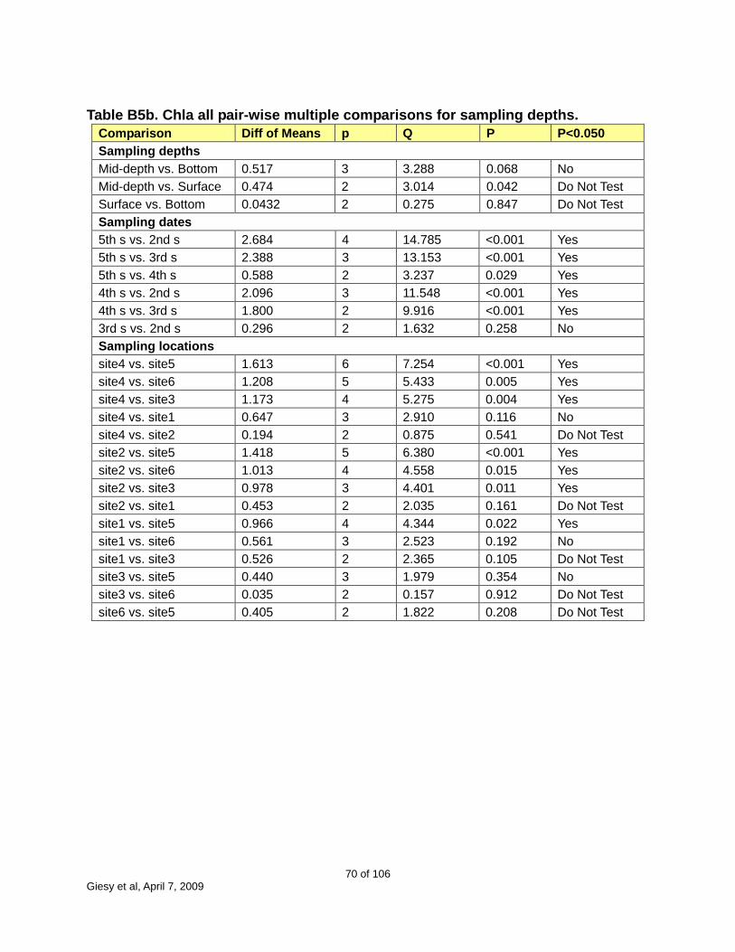
70 of 106 Giesy et al, April 7, 2009
Table B5b. Chla all pair-wise multiple comparisons for sampling depths.
Comparison Diff of Means p Q P P<0.050 Sampling depths Mid-depth vs. Bottom 0.517 3 3.288 0.068 No Mid-depth vs. Surface 0.474 2 3.014 0.042 Do Not Test Surface vs. Bottom 0.0432 2 0.275 0.847 Do Not Test Sampling dates 5th s vs. 2nd s 2.684 4 14.785 <0.001 Yes 5th s vs. 3rd s 2.388 3 13.153 <0.001 Yes 5th s vs. 4th s 0.588 2 3.237 0.029 Yes 4th s vs. 2nd s 2.096 3 11.548 <0.001 Yes 4th s vs. 3rd s 1.800 2 9.916 <0.001 Yes 3rd s vs. 2nd s 0.296 2 1.632 0.258 No Sampling locations site4 vs. site5 1.613 6 7.254 <0.001 Yes site4 vs. site6 1.208 5 5.433 0.005 Yes site4 vs. site3 1.173 4 5.275 0.004 Yes site4 vs. site1 0.647 3 2.910 0.116 No site4 vs. site2 0.194 2 0.875 0.541 Do Not Test site2 vs. site5 1.418 5 6.380 <0.001 Yes site2 vs. site6 1.013 4 4.558 0.015 Yes site2 vs. site3 0.978 3 4.401 0.011 Yes site2 vs. site1 0.453 2 2.035 0.161 Do Not Test site1 vs. site5 0.966 4 4.344 0.022 Yes site1 vs. site6 0.561 3 2.523 0.192 No site1 vs. site3 0.526 2 2.365 0.105 Do Not Test site3 vs. site5 0.440 3 1.979 0.354 No site3 vs. site6 0.035 2 0.157 0.912 Do Not Test site6 vs. site5 0.405 2 1.822 0.208 Do Not Test

71 of 106 Giesy et al, April 7, 2009
Table B5c. Least square means and Std Err of LS Mean of Chla.
Group Mean Least square means for sampling depths Surface 3.031 Mid-depth 3.505 Bottom 2.988 Std Err of LS Mean = 0.0185 Least square means for sampling dates 2nd s 1.905 3rd s 2.202 4th s 4.002 5th s 4.589 Std Err of LS Mean = 0.0214 Least square means for sampling locations site1 3.333 site2 3.786 site3 2.808 site4 3.980 site5 2.368 site6 2.773 Std Err of LS Mean = 0.0262
Table B6a. Result of three-way ANOVA of water column depth.
Source of Variation DF SS MS F P Sampling depths 2 5842.299 2921.149 56.094 <0.001 Sampling dates 3 156.701 52.234 1.003 0.405 Sampling locations 5 2371.452 474.290 9.108 <0.001 Residual 30 1562.286 52.076 Total 71 13919.444 196.049

72 of 106 Giesy et al, April 7, 2009
Table B6b. Depth of water column all pair-wise multiple comparisons.
Comparison Diff of Means p q P P<0.050 Sampling depths Bottom vs. Surface 22.036 3 14.96 <0.001 Yes Bottom vs. Mid-depth 11.991 2 8.140 <0.001 Yes Mid-depth vs. Surface 10.045 2 6.819 <0.001 Yes Sampling dates 2nd s vs. 5th s 4.114 4 2.419 0.336 No 2nd s vs. 4th s 1.886 3 1.109 0.716 Do Not Test 2nd s vs. 3rd s 1.455 2 0.856 0.550 Do Not Test 3rd s vs. 5th s 2.659 3 1.563 0.518 Do Not Test 3rd s vs. 4th s 0.431 2 0.253 0.859 Do Not Test 4th s vs. 5th s 2.228 2 1.31 0.362 Do Not Test Sampling locations site3 vs. site1 16.59 6 7.964 <0.001 Yes site3 vs. site4 10.655 5 5.115 0.009 Yes site3 vs. site6 10.519 4 5.049 0.006 Yes site3 vs. site2 3.646 3 1.750 0.441 No site3 vs. site5 2.498 2 1.199 0.403 Do Not Test site5 vs. site1 14.092 5 6.765 <0.001 Yes site5 vs. site4 8.157 4 3.916 0.045 Yes site5 vs. site6 8.021 3 3.85 0.028 Yes site5 vs. site2 1.148 2 0.551 0.700 Do Not Test site2 vs. site1 12.944 4 6.214 <0.001 Yes site2 vs. site4 7.009 3 3.365 0.060 No site2 vs. site6 6.873 2 3.299 0.027 Do Not Test site6 vs. site1 6.071 3 2.914 0.115 No site6 vs. site4 0.136 2 0.0653 0.964 Do Not Test site4 vs. site1 5.935 2 2.849 0.053 Do Not Test

73 of 106 Giesy et al, April 7, 2009
Table B6c. Least square means and Std Err of LS Mean of water column depth.
Group Mean Least square means for sampling depths Sampling depths 2.341 Sampling dates 12.386 Sampling locations 24.377 Std Err of LS Mean = 0.174 Least square means for sampling dates 2nd s 14.899 3rd s 13.443 4th s 13.013 5th s 10.784 Std Err of LS Mean = 0.200 Least square means for sampling locations site1 3.763 site2 16.707 site3 20.353 site4 9.698 site5 17.855 site6 9.834 Std Err of LS Mean = 0.246

74 of 106 Giesy et al, April 7, 2009
Appendix C. Tables of non-parametric analysis Table C1. Nonparametric analysis of Nitrite compared with sampling dates, locations and depths.
Kruskal-Wallis ANOVA by Ranks; Nitrite
Independent (grouping) variable: Sampling time
Kruskal-Wallis test: H ( 4, N= 81) =25.69515 p =.0000Depend.:Nitrite
Code ValidN
Sum ofRanks
samp1samp2samp3samp4samp5
101 5 171.0000102 19 943.0000103 19 977.5000104 19 884.5000105 19 345.0000
Median Test, Overall Median = .014570; Nitrite
Independent (grouping) variable: Sampling time
Chi-Square = 28.94996, df = 4, p = .0000Dependent:Nitrite
samp1 samp2 samp3 samp4 samp5 Total
<= Median: observedexpectedobs.-exp.
> Median: observedexpectedobs.-exp.
Total: observed
4.00000 6.00000 5.00000 7.00000 19.00000 41.000002.53086 9.61728 9.61728 9.61728 9.617281.46914 -3.61728 -4.61728 -2.61728 9.382721.00000 13.00000 14.00000 12.00000 0.00000 40.000002.46914 9.38272 9.38272 9.38272 9.38272
-1.46914 3.61728 4.61728 2.61728 -9.382725.00000 19.00000 19.00000 19.00000 19.00000 81.00000
Kruskal-Wallis ANOVA by Ranks; Nitrite
Independent (grouping) variable: Sampling site
Kruskal-Wallis test: H ( 6, N= 81) =4.224432 p =.6463Depend.:Nitrite
Code ValidN
Sum ofRanks
site1site2site3site4site5site6site7
101 13 512.0000102 13 407.0000103 13 547.0000104 13 573.0000105 12 561.0000106 13 591.0000107 4 130.0000
Median Test, Overall Median = .014570; Nitrite
Independent (grouping) variable: Sampling site
Chi-Square = 11.16884, df = 6, p = .0833Dependent:Nitrite
site1 site2 site3 site4 site5 site6 site7 Total
<= Median: observedexpectedobs.-exp.
> Median: observedexpectedobs.-exp.
Total: observed
7.00000 11.00000 8.00000 4.00000 5.00000 4.00000 2.000000 41.000006.58025 6.58025 6.58025 6.58025 6.07407 6.58025 2.0246910.41975 4.41975 1.41975 -2.58025 -1.07407 -2.58025 -0.0246916.00000 2.00000 5.00000 9.00000 7.00000 9.00000 2.000000 40.000006.41975 6.41975 6.41975 6.41975 5.92593 6.41975 1.975309
-0.41975 -4.41975 -1.41975 2.58025 1.07407 2.58025 0.02469113.00000 13.00000 13.00000 13.00000 12.00000 13.00000 4.000000 81.00000
Kruskal-Wallis ANOVA by Ranks; Nitrite Independent (grouping) variable: Sampling depth
Kruskal-Wallis test: H ( 2, N= 81) =.3624659 p =.8342Depend.:Nitrite
Code ValidN
Sum ofRanks
SurfaceMid DepthBottom111
104 33 1391.000105 24 1004.000109 24 926.000

75 of 106 Giesy et al, April 7, 2009
Median Test, Overall Median = .014570; Nitrite Independent (grouping) variable: Sampling depth
Chi-Square = .0179601, df = 2, p = .9911Dependent:Nitrite
Surface Mid Depth Bottom111 Total
<= Median: observedexpectedobs.-exp.
> Median: observedexpectedobs.-exp.
Total: observed
17.00000 12.00000 12.00000 41.0000016.70370 12.14815 12.148150.29630 -0.14815 -0.14815
16.00000 12.00000 12.00000 40.0000016.29630 11.85185 11.85185-0.29630 0.14815 0.1481533.00000 24.00000 24.00000 81.00000
Table C2. Nonparametric analysis of Nitrate compared with sampling dates, locations and depths.
Kruskal-Wallis ANOVA by Ranks; Nitrate Independent (grouping) variable: Sampling time
Kruskal-Wallis test: H ( 4, N= 81) =13.03092 p =.0111Depend.:Nitrate
Code ValidN
Sum ofRanks
samp1samp2samp3samp4samp5
101 5 321.0000102 19 885.0000103 19 606.5000104 19 606.5000105 19 902.0000
Median Test, Overall Median = .988491; Nitrate
Independent (grouping) variable: Sampling time
Chi-Square = 24.73879, df = 4, p = .0001Dependent:Nitrate
samp1 samp2 samp3 samp4 samp5 Total
<= Median: observedexpectedobs.-exp.
> Median: observedexpectedobs.-exp.
Total: observed
1.00000 7.00000 15.00000 15.00000 3.00000 41.000002.53086 9.61728 9.61728 9.61728 9.61728
-1.53086 -2.61728 5.38272 5.38272 -6.617284.00000 12.00000 4.00000 4.00000 16.00000 40.000002.46914 9.38272 9.38272 9.38272 9.382721.53086 2.61728 -5.38272 -5.38272 6.617285.00000 19.00000 19.00000 19.00000 19.00000 81.00000
Kruskal-Wallis ANOVA by Ranks; Nitrate Independent (grouping) variable: Sampling site
Kruskal-Wallis test: H ( 6, N= 81) =39.05261 p =.0000Depend.:Nitrate
Code ValidN
Sum ofRanks
site1site2site3site4site5site6site7
101 13 145.0000102 13 664.0000103 13 735.0000104 13 392.0000105 12 645.0000106 13 488.0000107 4 252.0000
Median Test, Overall Median = .988491; Nitrate
Independent (grouping) variable: Sampling site
Chi-Square = 21.09343, df = 6, p = .0018Dependent:Nitrate
site1 site2 site3 site4 site5 site6 site7 Total
<= Median: observedexpectedobs.-exp.
> Median: observedexpectedobs.-exp.
Total: observed
12.00000 4.00000 4.00000 9.00000 4.00000 8.00000 0.00000 41.000006.58025 6.58025 6.58025 6.58025 6.07407 6.58025 2.024695.41975 -2.58025 -2.58025 2.41975 -2.07407 1.41975 -2.024691.00000 9.00000 9.00000 4.00000 8.00000 5.00000 4.00000 40.000006.41975 6.41975 6.41975 6.41975 5.92593 6.41975 1.97531
-5.41975 2.58025 2.58025 -2.41975 2.07407 -1.41975 2.0246913.00000 13.00000 13.00000 13.00000 12.00000 13.00000 4.00000 81.00000
Kruskal-Wallis ANOVA by Ranks; Nitrate
Independent (grouping) variable: Sampling depth
Kruskal-Wallis test: H ( 2, N= 81) =3.821780 p =.1480Depend.:Nitrate
Code ValidN
Sum ofRanks
SurfaceMid DepthBottom111
104 33 1379.000105 24 813.000109 24 1129.000

76 of 106 Giesy et al, April 7, 2009
Median Test, Overall Median = .988491; Nitrate
Independent (grouping) variable: Sampling depth
Chi-Square = 2.184957, df = 2, p = .3354Dependent:Nitrate
Surface Mid Depth Bottom111 Total
<= Median: observedexpectedobs.-exp.
> Median: observedexpectedobs.-exp.
Total: observed
16.00000 15.00000 10.00000 41.0000016.70370 12.14815 12.14815-0.70370 2.85185 -2.1481517.00000 9.00000 14.00000 40.0000016.29630 11.85185 11.851850.70370 -2.85185 2.14815
33.00000 24.00000 24.00000 81.00000
Table C3. Nonparametric analysis of Sulfate compared with sampling dates, locations and depths.
Kruskal-Wallis ANOVA by Ranks; Sulphate Independent (grouping) variable: Sampling time
Kruskal-Wallis test: H ( 4, N= 81) =10.92943 p =.0274Depend.:Sulphate
Code ValidN
Sum ofRanks
samp1samp2samp3samp4samp5
101 5 178.0000102 19 959.0000103 19 618.5000104 19 618.5000105 19 947.0000
Median Test, Overall Median = 62.4250; Sulphate Independent (grouping) variable: Sampling time
Chi-Square = 10.50504, df = 4, p = .0327Dependent:Sulphate
samp1 samp2 samp3 samp4 samp5 Total
<= Median: observedexpectedobs.-exp.
> Median: observedexpectedobs.-exp.
Total: observed
3.000000 6.00000 13.00000 13.00000 6.00000 41.000002.530864 9.61728 9.61728 9.61728 9.617280.469136 -3.61728 3.38272 3.38272 -3.617282.000000 13.00000 6.00000 6.00000 13.00000 40.000002.469136 9.38272 9.38272 9.38272 9.38272
-0.469136 3.61728 -3.38272 -3.38272 3.617285.000000 19.00000 19.00000 19.00000 19.00000 81.00000
Kruskal-Wallis ANOVA by Ranks; Sulphate
Independent (grouping) variable: Sampling site
Kruskal-Wallis test: H ( 6, N= 81) =23.49088 p =.0006Depend.:Sulphate
Code ValidN
Sum ofRanks
site1site2site3site4site5site6site7
101 13 267.0000102 13 388.0000103 13 521.0000104 13 572.0000105 12 625.0000106 13 681.0000107 4 267.0000
Median Test, Overall Median = 62.4250; Sulphate
Independent (grouping) variable: Sampling site
Chi-Square = 21.09343, df = 6, p = .0018Dependent:Sulphate
site1 site2 site3 site4 site5 site6 site7 Total
<= Median: observedexpectedobs.-exp.
> Median: observedexpectedobs.-exp.
Total: observed
10.00000 10.00000 9.00000 6.00000 4.00000 2.00000 0.00000 41.000006.58025 6.58025 6.58025 6.58025 6.07407 6.58025 2.024693.41975 3.41975 2.41975 -0.58025 -2.07407 -4.58025 -2.024693.00000 3.00000 4.00000 7.00000 8.00000 11.00000 4.00000 40.000006.41975 6.41975 6.41975 6.41975 5.92593 6.41975 1.97531
-3.41975 -3.41975 -2.41975 0.58025 2.07407 4.58025 2.0246913.00000 13.00000 13.00000 13.00000 12.00000 13.00000 4.00000 81.00000

77 of 106 Giesy et al, April 7, 2009
Kruskal-Wallis ANOVA by Ranks; Sulphate Independent (grouping) variable: Sampling depth
Kruskal-Wallis test: H ( 2, N= 81) =5.142750 p =.0764Depend.:Sulphate
Code ValidN
Sum ofRanks
SurfaceMid DepthBottom111
104 33 1217.000105 24 901.000109 24 1203.000
Median Test, Overall Median = 62.4250; Sulphate Independent (grouping) variable: Sampling depth
Chi-Square = 6.306797, df = 2, p = .0427Dependent:Sulphate
Surface Mid Depth Bottom111 Total
<= Median: observedexpectedobs.-exp.
> Median: observedexpectedobs.-exp.
Total: observed
20.00000 14.00000 7.00000 41.0000016.70370 12.14815 12.148153.29630 1.85185 -5.14815
13.00000 10.00000 17.00000 40.0000016.29630 11.85185 11.85185-3.29630 -1.85185 5.1481533.00000 24.00000 24.00000 81.00000
Table C4. Nonparametric analysis of Chloride compared with sampling dates, locations and depths.
Kruskal-Wallis ANOVA by Ranks; ChlorideIndependent (grouping) variable: Sampling time
Kruskal-Wallis test: H ( 4, N= 81) =6.818893 p =.1458Depend.:Chloride
Code ValidN
Sum ofRanks
samp1samp2samp3samp4samp5
101 5 160.0000102 19 927.0000103 19 664.5000104 19 664.5000105 19 905.0000
Median Test, Overall Median = 7.64112; ChlorideIndependent (grouping) variable: Sampling time
Chi-Square = 5.451643, df = 4, p = .2440Dependent:Chloride
samp1 samp2 samp3 samp4 samp5 Total
<= Median: observedexpectedobs.-exp.
> Median: observedexpectedobs.-exp.
3.000000 7.00000 12.00000 12.00000 7.00000 41.000002.530864 9.61728 9.61728 9.61728 9.617280.469136 -2.61728 2.38272 2.38272 -2.617282.000000 12.00000 7.00000 7.00000 12.00000 40.000002.469136 9.38272 9.38272 9.38272 9.38272
-0.469136 2.61728 -2.38272 -2.38272 2.61728 Kruskal-Wallis ANOVA by Ranks; ChlorideIndependent (grouping) variable: Sampling site
Kruskal-Wallis test: H ( 6, N= 81) =31.68414 p =.0000Depend.:Chloride
Code ValidN
Sum ofRanks
site1site2site3site4site5site6site7
101 13 187.0000102 13 430.0000103 13 507.0000104 13 579.0000105 12 634.0000106 13 704.0000107 4 280.0000

78 of 106 Giesy et al, April 7, 2009
Median Test, Overall Median = 7.64112; Chloride Independent (grouping) variable: Sampling site
Chi-Square = 30.55641, df = 6, p = .0000Dependent:Chloride
site1 site2 site3 site4 site5 site6 site7 Total
<= Median: observedexpectedobs.-exp.
> Median: observedexpectedobs.-exp.
12.00000 9.00000 9.00000 6.00000 5.00000 0.00000 0.00000 41.000006.58025 6.58025 6.58025 6.58025 6.07407 6.58025 2.024695.41975 2.41975 2.41975 -0.58025 -1.07407 -6.58025 -2.024691.00000 4.00000 4.00000 7.00000 7.00000 13.00000 4.00000 40.000006.41975 6.41975 6.41975 6.41975 5.92593 6.41975 1.97531
-5.41975 -2.41975 -2.41975 0.58025 1.07407 6.58025 2.02469
Kruskal-Wallis ANOVA by Ranks; ChlorideIndependent (grouping) variable: Sampling depth
Kruskal-Wallis test: H ( 2, N= 81) =7.020093 p =.0299Depend.:Chloride
Code ValidN
Sum ofRanks
SurfaceMid DepthBottom111
104 33 1197.000105 24 884.000109 24 1240.000
Median Test, Overall Median = 7.64112; ChlorideIndependent (grouping) variable: Sampling depth
Chi-Square = 6.306797, df = 2, p = .0427Dependent:Chloride
Surface Mid Depth Bottom111 Total
<= Median: observedexpectedobs.-exp.
> Median: observedexpectedobs.-exp.
20.00000 14.00000 7.00000 41.0000016.70370 12.14815 12.148153.29630 1.85185 -5.14815
13.00000 10.00000 17.00000 40.0000016.29630 11.85185 11.85185-3.29630 -1.85185 5.14815
Table C5. Nonparametric analysis of PO4 compared with sampling dates, locations and depths.
Kruskal-Wallis ANOVA by Ranks; PO4
Independent (grouping) variable: Sampling time
Kruskal-Wallis test: H ( 4, N= 81) =14.78432 p =.0052Depend.:PO4
Code ValidN
Sum ofRanks
samp1samp2samp3samp4samp5
101 5 115.000102 19 667.000103 19 710.500104 19 1102.500105 19 726.000
Median Test, Overall Median = .008190; PO4 Independent (grouping) variable: Sampling time
Chi-Square = 16.73757, df = 4, p = .0022Dependent:PO4
samp1 samp2 samp3 samp4 samp5 Total
<= Median: observedexpectedobs.-exp.
> Median: observedexpectedobs.-exp.
Total: observed
4.00000 11.00000 12.00000 2.00000 12.00000 41.000002.53086 9.61728 9.61728 9.61728 9.617281.46914 1.38272 2.38272 -7.61728 2.382721.00000 8.00000 7.00000 17.00000 7.00000 40.000002.46914 9.38272 9.38272 9.38272 9.38272
-1.46914 -1.38272 -2.38272 7.61728 -2.382725.00000 19.00000 19.00000 19.00000 19.00000 81.00000
Kruskal-Wallis ANOVA by Ranks; PO4 Independent (grouping) variable: Sampling site
Kruskal-Wallis test: H ( 6, N= 81) =9.991740 p =.1250Depend.:PO4
Code ValidN
Sum ofRanks
site1site2site3site4site5site6site7
101 13 379.0000102 13 684.0000103 13 641.5000104 13 443.0000105 12 456.0000106 13 578.5000107 4 139.0000

79 of 106 Giesy et al, April 7, 2009
Median Test, Overall Median = .008190; PO4
Independent (grouping) variable: Sampling site
Chi-Square = 8.091452, df = 6, p = .2315Dependent:PO4
site1 site2 site3 site4 site5 site6 site7 Total
<= Median: observedexpectedobs.-exp.
> Median: observedexpectedobs.-exp.
Total: observed
10.00000 4.00000 4.00000 7.00000 7.00000 7.00000 2.000000 41.000006.58025 6.58025 6.58025 6.58025 6.07407 6.58025 2.0246913.41975 -2.58025 -2.58025 0.41975 0.92593 0.41975 -0.0246913.00000 9.00000 9.00000 6.00000 5.00000 6.00000 2.000000 40.000006.41975 6.41975 6.41975 6.41975 5.92593 6.41975 1.975309
-3.41975 2.58025 2.58025 -0.41975 -0.92593 -0.41975 0.02469113.00000 13.00000 13.00000 13.00000 12.00000 13.00000 4.000000 81.00000
Kruskal-Wallis ANOVA by Ranks; PO4
Independent (grouping) variable: Sampling depth
Kruskal-Wallis test: H ( 2, N= 81) =1.393921 p =.4981Depend.:PO4
Code ValidN
Sum ofRanks
SurfaceMid DepthBottom111
104 33 1324.000105 24 1092.000109 24 905.000
Median Test, Overall Median = .008190; PO4
Independent (grouping) variable: Sampling depth
Chi-Square = .3513442, df = 2, p = .8389Dependent:PO4
Surface Mid Depth Bottom111 Total
<= Median: observedexpectedobs.-exp.
> Median: observedexpectedobs.-exp.
Total: observed
17.00000 11.00000 13.00000 41.0000016.70370 12.14815 12.148150.29630 -1.14815 0.85185
16.00000 13.00000 11.00000 40.0000016.29630 11.85185 11.85185-0.29630 1.14815 -0.8518533.00000 24.00000 24.00000 81.00000
Table C6. Nonparametric analysis of Alkaklinity compared with sampling dates, locations and depths.
Kruskal-Wallis ANOVA by Ranks; Alkalinity Independent (grouping) variable: Sampling time
Kruskal-Wallis test: H ( 4, N= 81) =46.76607 p =.0000Depend.:Alkalinity
Code ValidN
Sum ofRanks
samp1samp2samp3samp4samp5
101 5 133.000102 19 531.000103 19 529.500104 19 759.500105 19 1368.000
Median Test, Overall Median = 142.000; Alkalinity
Independent (grouping) variable: Sampling time
Chi-Square = 38.66825, df = 4, p = .0000Dependent:Alkalinity
samp1 samp2 samp3 samp4 samp5 Total
<= Median: observedexpectedobs.-exp.
> Median: observedexpectedobs.-exp.
Total: observed
3.000000 15.00000 17.00000 7.00000 0.00000 42.000002.592593 9.85185 9.85185 9.85185 9.851850.407407 5.14815 7.14815 -2.85185 -9.851852.000000 4.00000 2.00000 12.00000 19.00000 39.000002.407407 9.14815 9.14815 9.14815 9.14815
-0.407407 -5.14815 -7.14815 2.85185 9.851855.000000 19.00000 19.00000 19.00000 19.00000 81.00000

80 of 106 Giesy et al, April 7, 2009
Kruskal-Wallis ANOVA by Ranks; Alkalinity Independent (grouping) variable: Sampling site
Kruskal-Wallis test: H ( 6, N= 81) =7.738347 p =.2579Depend.:Alkalinity
Code ValidN
Sum ofRanks
site1site2site3site4site5site6site7
101 13 333.0000102 13 531.5000103 13 529.0000104 13 606.0000105 12 580.5000106 13 559.0000107 4 182.0000
Median Test, Overall Median = 142.000; Alkalinity Independent (grouping) variable: Sampling site
Chi-Square = 7.591610, df = 6, p = .2696Dependent:Alkalinity
site1 site2 site3 site4 site5 site6 site7 Total
<= Median: observedexpectedobs.-exp.
> Median: observedexpectedobs.-exp.
Total: observed
10.00000 8.00000 6.00000 7.00000 3.00000 6.00000 2.000000 42.000006.74074 6.74074 6.74074 6.74074 6.22222 6.74074 2.0740743.25926 1.25926 -0.74074 0.25926 -3.22222 -0.74074 -0.0740743.00000 5.00000 7.00000 6.00000 9.00000 7.00000 2.000000 39.000006.25926 6.25926 6.25926 6.25926 5.77778 6.25926 1.925926
-3.25926 -1.25926 0.74074 -0.25926 3.22222 0.74074 0.07407413.00000 13.00000 13.00000 13.00000 12.00000 13.00000 4.000000 81.00000
Kruskal-Wallis ANOVA by Ranks; Alkalinity
Independent (grouping) variable: Sampling depth
Kruskal-Wallis test: H ( 2, N= 81) =3.063736 p =.2161Depend.:Alkalinity
Code ValidN
Sum ofRanks
SurfaceMid DepthBottom111
104 33 1178.500105 24 1031.000109 24 1111.500
Median Test, Overall Median = 142.000; Alkalinity
Independent (grouping) variable: Sampling depth
Chi-Square = 1.709416, df = 2, p = .4254Dependent:Alkalinity
Surface Mid Depth Bottom111 Total
<= Median: observedexpectedobs.-exp.
> Median: observedexpectedobs.-exp.
Total: observed
20.00000 11.00000 11.00000 42.0000017.11111 12.44444 12.444442.88889 -1.44444 -1.44444
13.00000 13.00000 13.00000 39.0000015.88889 11.55556 11.55556-2.88889 1.44444 1.4444433.00000 24.00000 24.00000 81.00000
Table C7. Nonparametric analysis of TN compared with sampling dates, locations and depths.
Kruskal-Wallis ANOVA by Ranks; TN Independent (grouping) variable: Sampling time
Kruskal-Wallis test: H ( 4, N= 81) =10.04015 p =.0398Depend.:TN
Code ValidN
Sum ofRanks
samp1samp2samp3samp4samp5
101 5 165.000102 19 610.500103 19 847.000104 19 681.000105 19 1017.500
Median Test, Overall Median = .432133; TN Independent (grouping) variable: Sampling time
Chi-Square = 15.05311, df = 4, p = .0046Dependent:TN
samp1 samp2 samp3 samp4 samp5 Total
<= Median: observedexpectedobs.-exp.
> Median: observedexpectedobs.-exp.
Total: observed
4.00000 14.00000 7.00000 12.00000 4.00000 41.000002.53086 9.61728 9.61728 9.61728 9.617281.46914 4.38272 -2.61728 2.38272 -5.617281.00000 5.00000 12.00000 7.00000 15.00000 40.000002.46914 9.38272 9.38272 9.38272 9.38272
-1.46914 -4.38272 2.61728 -2.38272 5.617285.00000 19.00000 19.00000 19.00000 19.00000 81.00000

81 of 106 Giesy et al, April 7, 2009
Kruskal-Wallis ANOVA by Ranks; TN
Independent (grouping) variable: Sampling site
Kruskal-Wallis test: H ( 6, N= 81) =34.17653 p =.0000Depend.:TN
Code ValidN
Sum ofRanks
site1site2site3site4site5site6site7
101 13 212.0000102 13 577.5000103 13 541.5000104 13 405.5000105 12 817.0000106 13 625.5000107 4 142.0000
Median Test, Overall Median = .432133; TN
Independent (grouping) variable: Sampling site
Chi-Square = 20.99085, df = 6, p = .0018Dependent:TN
site1 site2 site3 site4 site5 site6 site7 Total
<= Median: observedexpectedobs.-exp.
> Median: observedexpectedobs.-exp.
Total: observed
11.00000 7.00000 7.00000 9.00000 0.00000 5.00000 2.000000 41.000006.58025 6.58025 6.58025 6.58025 6.07407 6.58025 2.0246914.41975 0.41975 0.41975 2.41975 -6.07407 -1.58025 -0.0246912.00000 6.00000 6.00000 4.00000 12.00000 8.00000 2.000000 40.000006.41975 6.41975 6.41975 6.41975 5.92593 6.41975 1.975309
-4.41975 -0.41975 -0.41975 -2.41975 6.07407 1.58025 0.02469113.00000 13.00000 13.00000 13.00000 12.00000 13.00000 4.000000 81.00000
Kruskal-Wallis ANOVA by Ranks; TN Independent (grouping) variable: Sampling depth
Kruskal-Wallis test: H ( 2, N= 81) =3.475676 p =.1759Depend.:TN
Code ValidN
Sum ofRanks
SurfaceMid DepthBottom111
104 33 1196.500105 24 972.500109 24 1152.000
Median Test, Overall Median = .432133; TN
Independent (grouping) variable: Sampling depth
Chi-Square = 1.078728, df = 2, p = .5831Dependent:TN
Surface Mid Depth Bottom111 Total
<= Median: observedexpectedobs.-exp.
> Median: observedexpectedobs.-exp.
Total: observed
19.00000 11.00000 11.00000 41.0000016.70370 12.14815 12.148152.29630 -1.14815 -1.14815
14.00000 13.00000 13.00000 40.0000016.29630 11.85185 11.85185-2.29630 1.14815 1.1481533.00000 24.00000 24.00000 81.00000
Table C8. Nonparametric analysis of TP compared with sampling dates, locations and depths.
Kruskal-Wallis ANOVA by Ranks; TP Independent (grouping) variable: Sampling time
Kruskal-Wallis test: H ( 4, N= 81) =23.97533 p =.0001Depend.:TP
Code ValidN
Sum ofRanks
samp1samp2samp3samp4samp5
101 5 133.000102 19 533.000103 19 627.000104 19 875.500105 19 1152.500

82 of 106 Giesy et al, April 7, 2009
Median Test, Overall Median = .014579; TP
Independent (grouping) variable: Sampling time
Chi-Square = 14.63199, df = 4, p = .0055Dependent:TP
samp1 samp2 samp3 samp4 samp5 Total
<= Median: observedexpectedobs.-exp.
> Median: observedexpectedobs.-exp.
Total: observed
4.00000 13.00000 13.00000 7.00000 4.00000 41.000002.53086 9.61728 9.61728 9.61728 9.617281.46914 3.38272 3.38272 -2.61728 -5.617281.00000 6.00000 6.00000 12.00000 15.00000 40.000002.46914 9.38272 9.38272 9.38272 9.38272
-1.46914 -3.38272 -3.38272 2.61728 5.617285.00000 19.00000 19.00000 19.00000 19.00000 81.00000
Kruskal-Wallis ANOVA by Ranks; TP Independent (grouping) variable: Sampling site
Kruskal-Wallis test: H ( 6, N= 81) =9.129099 p =.1665Depend.:TP
Code ValidN
Sum ofRanks
site1site2site3site4site5site6site7
101 13 652.5000102 13 503.0000103 13 421.0000104 13 403.0000105 12 490.5000106 13 677.0000107 4 174.0000
Median Test, Overall Median = .014579; TP Independent (grouping) variable: Sampling site
Chi-Square = 6.014212, df = 6, p = .4216Dependent:TP
site1 site2 site3 site4 site5 site6 site7 Total
<= Median: observedexpectedobs.-exp.
> Median: observedexpectedobs.-exp.
Total: observed
5.00000 8.00000 8.00000 8.00000 7.00000 4.00000 1.00000 41.000006.58025 6.58025 6.58025 6.58025 6.07407 6.58025 2.02469
-1.58025 1.41975 1.41975 1.41975 0.92593 -2.58025 -1.024698.00000 5.00000 5.00000 5.00000 5.00000 9.00000 3.00000 40.000006.41975 6.41975 6.41975 6.41975 5.92593 6.41975 1.975311.58025 -1.41975 -1.41975 -1.41975 -0.92593 2.58025 1.02469
13.00000 13.00000 13.00000 13.00000 12.00000 13.00000 4.00000 81.00000
Kruskal-Wallis ANOVA by Ranks; TP
Independent (grouping) variable: Sampling depth
Kruskal-Wallis test: H ( 2, N= 81) =.9744009 p =.6143Depend.:TP
Code ValidN
Sum ofRanks
SurfaceMid DepthBottom111
104 33 1251.500105 24 1047.000109 24 1022.500
Median Test, Overall Median = .014579; TP
Independent (grouping) variable: Sampling depth
Chi-Square = 1.412112, df = 2, p = .4936Dependent:TP
Surface Mid Depth Bottom111 Total
<= Median: observedexpectedobs.-exp.
> Median: observedexpectedobs.-exp.
Total: observed
19.00000 10.00000 12.00000 41.0000016.70370 12.14815 12.148152.29630 -2.14815 -0.14815
14.00000 14.00000 12.00000 40.0000016.29630 11.85185 11.85185-2.29630 2.14815 0.1481533.00000 24.00000 24.00000 81.00000
Table C9. Nonparametric analysis of Mn compared with sampling dates, locations and depths.

83 of 106 Giesy et al, April 7, 2009
Kruskal-Wallis ANOVA by Ranks; Mn Independent (grouping) variable: Sampling time
Kruskal-Wallis test: H ( 4, N= 81) =24.51384 p =.0001Depend.:Mn
Code ValidN
Sum ofRanks
samp1samp2samp3samp4samp5
101 5 390.0000102 19 965.5000103 19 826.5000104 19 607.5000105 19 531.5000
Median Test, Overall Median = .427000; Mn
Independent (grouping) variable: Sampling time
Chi-Square = 19.93806, df = 4, p = .0005Dependent:Mn
samp1 samp2 samp3 samp4 samp5 Total
<= Median: observedexpectedobs.-exp.
> Median: observedexpectedobs.-exp.
Total: observed
0.00000 5.00000 8.00000 12.00000 16.00000 41.000002.53086 9.61728 9.61728 9.61728 9.61728
-2.53086 -4.61728 -1.61728 2.38272 6.382725.00000 14.00000 11.00000 7.00000 3.00000 40.000002.46914 9.38272 9.38272 9.38272 9.382722.53086 4.61728 1.61728 -2.38272 -6.382725.00000 19.00000 19.00000 19.00000 19.00000 81.00000
Kruskal-Wallis ANOVA by Ranks; Mn
Independent (grouping) variable: Sampling site
Kruskal-Wallis test: H ( 6, N= 81) =13.85092 p =.0313Depend.:Mn
Code ValidN
Sum ofRanks
site1site2site3site4site5site6site7
101 13 651.5000102 13 612.5000103 13 509.0000104 13 660.0000105 12 376.5000106 13 319.5000107 4 192.0000
Median Test, Overall Median = .427000; Mn
Independent (grouping) variable: Sampling site
Chi-Square = 10.32256, df = 6, p = .1117Dependent:Mn
site1 site2 site3 site4 site5 site6 site7 Total
<= Median: observedexpectedobs.-exp.
> Median: observedexpectedobs.-exp.
Total: observed
6.00000 4.00000 7.00000 5.00000 7.00000 11.00000 1.00000 41.000006.58025 6.58025 6.58025 6.58025 6.07407 6.58025 2.02469
-0.58025 -2.58025 0.41975 -1.58025 0.92593 4.41975 -1.024697.00000 9.00000 6.00000 8.00000 5.00000 2.00000 3.00000 40.000006.41975 6.41975 6.41975 6.41975 5.92593 6.41975 1.975310.58025 2.58025 -0.41975 1.58025 -0.92593 -4.41975 1.02469
13.00000 13.00000 13.00000 13.00000 12.00000 13.00000 4.00000 81.00000
Kruskal-Wallis ANOVA by Ranks; Mn
Independent (grouping) variable: Sampling depth
Kruskal-Wallis test: H ( 2, N= 81) =6.930849 p =.0313Depend.:Mn
Code ValidN
Sum ofRanks
SurfaceMid DepthBottom111
104 33 1497.500105 24 729.500109 24 1094.000
Median Test, Overall Median = .427000; Mn Independent (grouping) variable: Sampling depth
Chi-Square = 2.184957, df = 2, p = .3354Dependent:Mn
Surface Mid Depth Bottom111 Total
<= Median: observedexpectedobs.-exp.
> Median: observedexpectedobs.-exp.
Total: observed
16.00000 15.00000 10.00000 41.0000016.70370 12.14815 12.14815-0.70370 2.85185 -2.1481517.00000 9.00000 14.00000 40.0000016.29630 11.85185 11.851850.70370 -2.85185 2.14815
33.00000 24.00000 24.00000 81.00000

84 of 106 Giesy et al, April 7, 2009
Table C10. Nonparametric analysis of Fe compared with sampling dates, locations and depths.
Kruskal-Wallis ANOVA by Ranks; Fe
Independent (grouping) variable: Sampling time
Kruskal-Wallis test: H ( 4, N= 81) =47.77958 p =.0000Depend.:Fe
Code ValidN
Sum ofRanks
samp1samp2samp3samp4samp5
101 5 395.000102 19 1106.000103 19 864.000104 19 665.000105 19 291.000
Median Test, Overall Median = 1.56300; Fe Independent (grouping) variable: Sampling time
Chi-Square = 30.88710, df = 4, p = .0000Dependent:Fe
samp1 samp2 samp3 samp4 samp5 Total
<= Median: observedexpectedobs.-exp.
> Median: observedexpectedobs.-exp.
Total: observed
0.00000 3.00000 8.00000 12.00000 18.00000 41.000002.53086 9.61728 9.61728 9.61728 9.61728
-2.53086 -6.61728 -1.61728 2.38272 8.382725.00000 16.00000 11.00000 7.00000 1.00000 40.000002.46914 9.38272 9.38272 9.38272 9.382722.53086 6.61728 1.61728 -2.38272 -8.382725.00000 19.00000 19.00000 19.00000 19.00000 81.00000
Kruskal-Wallis ANOVA by Ranks; Fe Independent (grouping) variable: Sampling site
Kruskal-Wallis test: H ( 6, N= 81) =14.45417 p =.0250Depend.:Fe
Code ValidN
Sum ofRanks
site1site2site3site4site5site6site7
101 13 785.0000102 13 526.0000103 13 483.0000104 13 587.0000105 12 423.0000106 13 430.0000107 4 87.0000
Median Test, Overall Median = 1.56300; Fe Independent (grouping) variable: Sampling site
Chi-Square = 13.09221, df = 6, p = .0416Dependent:Fe
site1 site2 site3 site4 site5 site6 site7 Total
<= Median: observedexpectedobs.-exp.
> Median: observedexpectedobs.-exp.
Total: observed
2.00000 7.00000 7.00000 5.00000 8.00000 8.00000 4.00000 41.000006.58025 6.58025 6.58025 6.58025 6.07407 6.58025 2.02469
-4.58025 0.41975 0.41975 -1.58025 1.92593 1.41975 1.9753111.00000 6.00000 6.00000 8.00000 4.00000 5.00000 0.00000 40.000006.41975 6.41975 6.41975 6.41975 5.92593 6.41975 1.975314.58025 -0.41975 -0.41975 1.58025 -1.92593 -1.41975 -1.97531
13.00000 13.00000 13.00000 13.00000 12.00000 13.00000 4.00000 81.00000
Kruskal-Wallis ANOVA by Ranks; Fe
Independent (grouping) variable: Sampling depth
Kruskal-Wallis test: H ( 2, N= 81) =.2601284 p =.8780Depend.:Fe
Code ValidN
Sum ofRanks
SurfaceMid DepthBottom111
104 33 1356.000105 24 941.000109 24 1024.000
Median Test, Overall Median = 1.56300; Fe
Independent (grouping) variable: Sampling depth
Chi-Square = .4271134, df = 2, p = .8077Dependent:Fe
Surface Mid Depth Bottom111 Total
<= Median: observedexpectedobs.-exp.
> Median: observedexpectedobs.-exp.
Total: observed
18.00000 12.00000 11.00000 41.0000016.70370 12.14815 12.148151.29630 -0.14815 -1.14815
15.00000 12.00000 13.00000 40.0000016.29630 11.85185 11.85185-1.29630 0.14815 1.1481533.00000 24.00000 24.00000 81.00000

85 of 106 Giesy et al, April 7, 2009
Table C11. Nonparametric analysis of TurbSC compared with sampling dates, locations and depths.
Kruskal-Wallis ANOVA by Ranks; TurbSC
Independent (grouping) variable: Sampling time
Kruskal-Wallis test: H ( 4, N= 81) =67.87952 p =.0000Depend.:TurbSC
Code ValidN
Sum ofRanks
samp1samp2samp3samp4samp5
101 5 200.000102 19 277.000103 19 1012.000104 19 1346.000105 19 486.000
Median Test, Overall Median = 27.9333; TurbSC Independent (grouping) variable: Sampling time
Chi-Square = 66.85047, df = 4, p = .0000Dependent:TurbSC
samp1 samp2 samp3 samp4 samp5 Total
<= Median: observedexpectedobs.-exp.
> Median: observedexpectedobs.-exp.
Total: observed
4.00000 17.00000 1.00000 0.00000 19.00000 41.000002.53086 9.61728 9.61728 9.61728 9.617281.46914 7.38272 -8.61728 -9.61728 9.382721.00000 2.00000 18.00000 19.00000 0.00000 40.000002.46914 9.38272 9.38272 9.38272 9.38272
-1.46914 -7.38272 8.61728 9.61728 -9.382725.00000 19.00000 19.00000 19.00000 19.00000 81.00000
Kruskal-Wallis ANOVA by Ranks; TurbSC Independent (grouping) variable: Sampling site
Kruskal-Wallis test: H ( 6, N= 81) =1.595880 p =.9529Depend.:TurbSC
Code ValidN
Sum ofRanks
site1site2site3site4site5site6site7
101 13 615.5000102 13 549.5000103 13 532.0000104 13 534.0000105 12 449.5000106 13 489.0000107 4 151.5000 Median Test, Overall Median = 27.9333; TurbSC Independent (grouping) variable: Sampling site
Chi-Square = .9878049, df = 6, p = .9861Dependent:TurbSC
site1 site2 site3 site4 site5 site6 site7 Total
<= Median: observedexpectedobs.-exp.
> Median: observedexpectedobs.-exp.
Total: observed
5.00000 7.00000 7.00000 7.00000 6.00000 7.00000 2.000000 41.000006.58025 6.58025 6.58025 6.58025 6.07407 6.58025 2.024691
-1.58025 0.41975 0.41975 0.41975 -0.07407 0.41975 -0.0246918.00000 6.00000 6.00000 6.00000 6.00000 6.00000 2.000000 40.000006.41975 6.41975 6.41975 6.41975 5.92593 6.41975 1.9753091.58025 -0.41975 -0.41975 -0.41975 0.07407 -0.41975 0.024691
13.00000 13.00000 13.00000 13.00000 12.00000 13.00000 4.000000 81.00000
Kruskal-Wallis ANOVA by Ranks; TurbSC Independent (grouping) variable: Sampling depth
Kruskal-Wallis test: H ( 2, N= 81) =.2020413 p =.9039Depend.:TurbSC
Code ValidN
Sum ofRanks
SurfaceMid DepthBottom111
104 33 1308.500105 24 995.000109 24 1017.500

86 of 106 Giesy et al, April 7, 2009
Median Test, Overall Median = 27.9333; TurbSC
Independent (grouping) variable: Sampling depth
Chi-Square = .4271134, df = 2, p = .8077Dependent:TurbSC
Surface Mid Depth Bottom111 Total
<= Median: observedexpectedobs.-exp.
> Median: observedexpectedobs.-exp.
Total: observed
18.00000 12.00000 11.00000 41.0000016.70370 12.14815 12.148151.29630 -0.14815 -1.14815
15.00000 12.00000 13.00000 40.0000016.29630 11.85185 11.85185-1.29630 0.14815 1.1481533.00000 24.00000 24.00000 81.00000
Table C12. Nonparametric analysis of Temp compared with sampling dates, locations and depths.
Kruskal-Wallis ANOVA by Ranks; Temp Independent (grouping) variable: Sampling time
Kruskal-Wallis test: H ( 4, N= 81) =24.75825 p =.0001Depend.:Temp
Code ValidN
Sum ofRanks
samp1samp2samp3samp4samp5
101 5 315.5000102 19 974.0000103 19 979.0000104 19 590.0000105 19 462.5000 Median Test, Overall Median = 15.1100; Temp Independent (grouping) variable: Sampling time
Chi-Square = 45.20507, df = 4, p = .0000Dependent:Temp
samp1 samp2 samp3 samp4 samp5 Total
<= Median: observedexpectedobs.-exp.
> Median: observedexpectedobs.-exp.
Total: observed
0.00000 5.00000 2.00000 18.00000 16.00000 41.000002.53086 9.61728 9.61728 9.61728 9.61728
-2.53086 -4.61728 -7.61728 8.38272 6.382725.00000 14.00000 17.00000 1.00000 3.00000 40.000002.46914 9.38272 9.38272 9.38272 9.382722.53086 4.61728 7.61728 -8.38272 -6.382725.00000 19.00000 19.00000 19.00000 19.00000 81.00000
Kruskal-Wallis ANOVA by Ranks; Temp
Independent (grouping) variable: Sampling site
Kruskal-Wallis test: H ( 6, N= 81) =9.916580 p =.1282Depend.:Temp
Code ValidN
Sum ofRanks
site1site2site3site4site5site6site7
101 13 743.5000102 13 481.0000103 13 399.0000104 13 564.5000105 12 429.0000106 13 554.0000107 4 150.0000
Median Test, Overall Median = 15.1100; Temp Independent (grouping) variable: Sampling site
Chi-Square = 8.758220, df = 6, p = .1876Dependent:Temp
site1 site2 site3 site4 site5 site6 site7 Total
<= Median: observedexpectedobs.-exp.
> Median: observedexpectedobs.-exp.
Total: observed
3.00000 7.00000 10.00000 6.00000 6.00000 6.00000 3.000000 41.000006.58025 6.58025 6.58025 6.58025 6.07407 6.58025 2.024691
-3.58025 0.41975 3.41975 -0.58025 -0.07407 -0.58025 0.97530910.00000 6.00000 3.00000 7.00000 6.00000 7.00000 1.000000 40.000006.41975 6.41975 6.41975 6.41975 5.92593 6.41975 1.9753093.58025 -0.41975 -3.41975 0.58025 0.07407 0.58025 -0.975309
13.00000 13.00000 13.00000 13.00000 12.00000 13.00000 4.000000 81.00000
Kruskal-Wallis ANOVA by Ranks; Temp Independent (grouping) variable: Sampling depth
Kruskal-Wallis test: H ( 2, N= 81) =6.181288 p =.0455Depend.:Temp
Code ValidN
Sum ofRanks
SurfaceMid DepthBottom111
104 33 1554.000105 24 1011.000109 24 756.000

87 of 106 Giesy et al, April 7, 2009
Median Test, Overall Median = 15.1100; Temp Independent (grouping) variable: Sampling depth
Chi-Square = 2.245572, df = 2, p = .3254Dependent:Temp
Surface Mid Depth Bottom111 Total
<= Median: observedexpectedobs.-exp.
> Median: observedexpectedobs.-exp.
Total: observed
14.00000 12.00000 15.00000 41.0000016.70370 12.14815 12.14815-2.70370 -0.14815 2.8518519.00000 12.00000 9.00000 40.0000016.29630 11.85185 11.851852.70370 0.14815 -2.85185
33.00000 24.00000 24.00000 81.00000 Table C13. Nonparametric analysis of SpCond compared with sampling dates, locations and depths.
Kruskal-Wallis ANOVA by Ranks; SpCond Independent (grouping) variable: Sampling time
Kruskal-Wallis test: H ( 4, N= 81) =9.197763 p =.0563Depend.:SpCond
Code ValidN
Sum ofRanks
samp1samp2samp3samp4samp5
101 5 156.0000102 19 860.5000103 19 630.5000104 19 675.5000105 19 998.5000
Median Test, Overall Median = 426.100; SpCond Independent (grouping) variable: Sampling time
Chi-Square = 14.71621, df = 4, p = .0053Dependent:SpCond
samp1 samp2 samp3 samp4 samp5 Total
<= Median: observedexpectedobs.-exp.
> Median: observedexpectedobs.-exp.
Total: observed
3.000000 9.00000 14.00000 12.00000 3.00000 41.000002.530864 9.61728 9.61728 9.61728 9.617280.469136 -0.61728 4.38272 2.38272 -6.617282.000000 10.00000 5.00000 7.00000 16.00000 40.000002.469136 9.38272 9.38272 9.38272 9.38272
-0.469136 0.61728 -4.38272 -2.38272 6.617285.000000 19.00000 19.00000 19.00000 19.00000 81.00000
Kruskal-Wallis ANOVA by Ranks; SpCond Independent (grouping) variable: Sampling site
Kruskal-Wallis test: H ( 6, N= 81) =11.08804 p =.0857Depend.:SpCond
Code ValidN
Sum ofRanks
site1site2site3site4site5site6site7
101 13 369.0000102 13 376.5000103 13 600.0000104 13 567.5000105 12 595.0000106 13 607.0000107 4 206.0000
Median Test, Overall Median = 426.100; SpCond Independent (grouping) variable: Sampling site
Chi-Square = 9.091604, df = 6, p = .1685Dependent:SpCond
site1 site2 site3 site4 site5 site6 site7 Total
<= Median: observedexpectedobs.-exp.
> Median: observedexpectedobs.-exp.
Total: observed
10.00000 8.00000 5.00000 8.00000 5.00000 4.00000 1.00000 41.000006.58025 6.58025 6.58025 6.58025 6.07407 6.58025 2.024693.41975 1.41975 -1.58025 1.41975 -1.07407 -2.58025 -1.024693.00000 5.00000 8.00000 5.00000 7.00000 9.00000 3.00000 40.000006.41975 6.41975 6.41975 6.41975 5.92593 6.41975 1.97531
-3.41975 -1.41975 1.58025 -1.41975 1.07407 2.58025 1.0246913.00000 13.00000 13.00000 13.00000 12.00000 13.00000 4.00000 81.00000
Kruskal-Wallis ANOVA by Ranks; SpCond Independent (grouping) variable: Sampling depth
Kruskal-Wallis test: H ( 2, N= 81) =4.465486 p =.1072Depend.:SpCond
Code ValidN
Sum ofRanks
SurfaceMid DepthBottom111
104 33 1251.500105 24 882.000109 24 1187.500

88 of 106 Giesy et al, April 7, 2009
Median Test, Overall Median = 426.100; SpCond
Independent (grouping) variable: Sampling depth
Chi-Square = 4.079185, df = 2, p = .1301Dependent:SpCond
Surface Mid Depth Bottom111 Total
<= Median: observedexpectedobs.-exp.
> Median: observedexpectedobs.-exp.
Total: observed
19.00000 14.00000 8.00000 41.0000016.70370 12.14815 12.148152.29630 1.85185 -4.14815
14.00000 10.00000 16.00000 40.0000016.29630 11.85185 11.85185-2.29630 -1.85185 4.1481533.00000 24.00000 24.00000 81.00000
Table C14. Nonparametric analysis of TDS compared with sampling dates, locations and depths.
Kruskal-Wallis ANOVA by Ranks; TDS Independent (grouping) variable: Sampling time
Kruskal-Wallis test: H ( 4, N= 81) =29.18018 p =.0000Depend.:TDS
Code ValidN
Sum ofRanks
samp1samp2samp3samp4samp5
101 5 115.000102 19 628.000103 19 1033.000104 19 1079.000105 19 466.000
Median Test, Overall Median = .285133; TDS
Independent (grouping) variable: Sampling time
Chi-Square = 39.56211, df = 4, p = .0000Dependent:TDS
samp1 samp2 samp3 samp4 samp5 Total
<= Median: observedexpectedobs.-exp.
> Median: observedexpectedobs.-exp.
Total: observed
3.000000 13.00000 3.00000 3.00000 19.00000 41.000002.530864 9.61728 9.61728 9.61728 9.617280.469136 3.38272 -6.61728 -6.61728 9.382722.000000 6.00000 16.00000 16.00000 0.00000 40.000002.469136 9.38272 9.38272 9.38272 9.38272
-0.469136 -3.38272 6.61728 6.61728 -9.382725.000000 19.00000 19.00000 19.00000 19.00000 81.00000
Kruskal-Wallis ANOVA by Ranks; TDS
Independent (grouping) variable: Sampling site
Kruskal-Wallis test: H ( 6, N= 81) =10.57579 p =.1024Depend.:TDS
Code ValidN
Sum ofRanks
site1site2site3site4site5site6site7
101 13 626.0000102 13 314.0000103 13 558.0000104 13 553.0000105 12 554.0000106 13 490.5000107 4 225.5000
Median Test, Overall Median = .285133; TDS
Independent (grouping) variable: Sampling site
Chi-Square = 9.373698, df = 6, p = .1536Dependent:TDS
site1 site2 site3 site4 site5 site6 site7 Total
<= Median: observedexpectedobs.-exp.
> Median: observedexpectedobs.-exp.
Total: observed
4.00000 10.00000 5.00000 6.00000 6.00000 9.00000 1.00000 41.000006.58025 6.58025 6.58025 6.58025 6.07407 6.58025 2.02469
-2.58025 3.41975 -1.58025 -0.58025 -0.07407 2.41975 -1.024699.00000 3.00000 8.00000 7.00000 6.00000 4.00000 3.00000 40.000006.41975 6.41975 6.41975 6.41975 5.92593 6.41975 1.975312.58025 -3.41975 1.58025 0.58025 0.07407 -2.41975 1.02469
13.00000 13.00000 13.00000 13.00000 12.00000 13.00000 4.00000 81.00000

89 of 106 Giesy et al, April 7, 2009
Kruskal-Wallis ANOVA by Ranks; TDS Independent (grouping) variable: Sampling depth
Kruskal-Wallis test: H ( 2, N= 81) =1.558801 p =.4587Depend.:TDS
Code ValidN
Sum ofRanks
SurfaceMid DepthBottom111
104 33 1294.000105 24 923.000109 24 1104.000
Median Test, Overall Median = .285133; TDS Independent (grouping) variable: Sampling depth
Chi-Square = .1846522, df = 2, p = .9118Dependent:TDS
Surface Mid Depth Bottom111 Total
<= Median: observedexpectedobs.-exp.
> Median: observedexpectedobs.-exp.
Total: observed
16.00000 13.00000 12.00000 41.0000016.70370 12.14815 12.14815-0.70370 0.85185 -0.1481517.00000 11.00000 12.00000 40.0000016.29630 11.85185 11.851850.70370 -0.85185 0.14815
33.00000 24.00000 24.00000 81.00000
Table C15. Nonparametric analysis of Salinity compared with sampling dates, locations and depths.
Kruskal-Wallis ANOVA by Ranks; Salinity
Independent (grouping) variable: Sampling time
Kruskal-Wallis test: H ( 4, N= 81) =2.114678 p =.7147Depend.:Salinity
Code ValidN
Sum ofRanks
samp1samp2samp3samp4samp5
101 5 165.0000102 19 711.5000103 19 808.0000104 19 869.0000105 19 767.5000
Median Test, Overall Median = .210000; Salinity
Independent (grouping) variable: Sampling time
Chi-Square = .8867368, df = 4, p = .9265Dependent:Salinity
samp1 samp2 samp3 samp4 samp5 Total
<= Median: observedexpectedobs.-exp.
> Median: observedexpectedobs.-exp.
Total: observed
3.000000 14.00000 14.00000 12.00000 13.00000 56.000003.456790 13.13580 13.13580 13.13580 13.13580
-0.456790 0.86420 0.86420 -1.13580 -0.135802.000000 5.00000 5.00000 7.00000 6.00000 25.000001.543210 5.86420 5.86420 5.86420 5.864200.456790 -0.86420 -0.86420 1.13580 0.135805.000000 19.00000 19.00000 19.00000 19.00000 81.00000
Kruskal-Wallis ANOVA by Ranks; Salinity Independent (grouping) variable: Sampling site
Kruskal-Wallis test: H ( 6, N= 81) =28.41021 p =.0001Depend.:Salinity
Code ValidN
Sum ofRanks
site1site2site3site4site5site6site7
101 13 213.5000102 13 485.0000103 13 671.5000104 13 439.0000105 12 625.0000106 13 700.0000107 4 187.0000

90 of 106 Giesy et al, April 7, 2009
Median Test, Overall Median = .210000; Salinity Independent (grouping) variable: Sampling site
Chi-Square = 19.71593, df = 6, p = .0031Dependent:Salinity
site1 site2 site3 site4 site5 site6 site7 Total
<= Median: observedexpectedobs.-exp.
> Median: observedexpectedobs.-exp.
Total: observed
13.00000 11.00000 6.00000 12.00000 6.00000 6.00000 2.000000 56.000008.98765 8.98765 8.98765 8.98765 8.29630 8.98765 2.7654324.01235 2.01235 -2.98765 3.01235 -2.29630 -2.98765 -0.7654320.00000 2.00000 7.00000 1.00000 6.00000 7.00000 2.000000 25.000004.01235 4.01235 4.01235 4.01235 3.70370 4.01235 1.234568
-4.01235 -2.01235 2.98765 -3.01235 2.29630 2.98765 0.76543213.00000 13.00000 13.00000 13.00000 12.00000 13.00000 4.000000 81.00000
Kruskal-Wallis ANOVA by Ranks; Salinity Independent (grouping) variable: Sampling depth
Kruskal-Wallis test: H ( 2, N= 81) =3.910323 p =.1415Depend.:Salinity
Code ValidN
Sum ofRanks
SurfaceMid DepthBottom111
104 33 1210.500105 24 952.500109 24 1158.000
Median Test, Overall Median = .210000; Salinity
Independent (grouping) variable: Sampling depth
Chi-Square = 3.585170, df = 2, p = .1665Dependent:Salinity
Surface Mid Depth Bottom111 Total
<= Median: observedexpectedobs.-exp.
> Median: observedexpectedobs.-exp.
Total: observed
25.00000 18.00000 13.00000 56.0000022.81481 16.59259 16.592592.18519 1.40741 -3.592598.00000 6.00000 11.00000 25.00000
10.18519 7.40741 7.40741-2.18519 -1.40741 3.5925933.00000 24.00000 24.00000 81.00000

91 of 106 Giesy et al, April 7, 2009
Appendix D. Figures of box plots (non-parametric analysis).
Boxplot by Group
Variable: Nitrite
Median 25%-75% Min-Max
samp1 samp2 samp3 samp4 samp5Sampling time
0.00
0.02
0.04
0.06
0.08
0.10
0.12
0.14
Nitri
te
Boxplot by Group
Variable: Nitrite
Median 25%-75% Min-Max
site1 site2 site3 site4 site5 site6 site7Sampling site
0.00
0.02
0.04
0.06
0.08
0.10
0.12
0.14
Nitr
ite
Boxplot by Group
Variable: Nitrite
Median 25%-75% Min-Max
Surface Mid Depth Bottom111Sampling depth
0.00
0.02
0.04
0.06
0.08
0.10
0.12
0.14
Nitr
ite
Fig. D1. Box plots of Nitrite compared with sampling dates, locations and depths.

92 of 106 Giesy et al, April 7, 2009
Boxplot by Group
Variable: Nitrate
Median 25%-75% Min-Max
samp1 samp2 samp3 samp4 samp5Sampling time
0.0
0.2
0.4
0.6
0.8
1.0
1.2
1.4
1.6
1.8
2.0
Nitr
ate
Boxplot by Group
Variable: Nitrate
Median 25%-75% Min-Max
site1 site2 site3 site4 site5 site6 site7Sampling site
0.0
0.2
0.4
0.6
0.8
1.0
1.2
1.4
1.6
1.8
2.0
Nitr
ate
Boxplot by Group
Variable: Nitrate
Median 25%-75% Min-Max
Surface Mid Depth Bottom111Sampling depth
0.0
0.2
0.4
0.6
0.8
1.0
1.2
1.4
1.6
1.8
2.0
Nitr
ate
Fig. D2. Box plots of Nitrate compared with sampling dates, locations and depths.

93 of 106 Giesy et al, April 7, 2009
Boxplot by Group
Variable: Sulphate
Median 25%-75% Min-Max
samp1 samp2 samp3 samp4 samp5Sampling time
46
48
50
52
54
56
58
60
62
64
66
68
70
72
Sulp
hate
Boxplot by Group
Variable: Sulphate
Median 25%-75% Min-Max
site1 site2 site3 site4 site5 site6 site7Sampling site
46
48
50
52
54
56
58
60
62
64
66
68
70
72
Sulp
hate
Boxplot by Group
Variable: Sulphate
Median 25%-75% Min-Max
Surface Mid Depth Bottom111Sampling depth
46
48
50
52
54
56
58
60
62
64
66
68
70
72
Sulp
hate
Fig. D3. Box plots of Sulfate compared with sampling dates, locations and depths.

94 of 106 Giesy et al, April 7, 2009
Fig. D4. Box plots of Chloride compared with sampling dates, locations and depths.
Boxplot by GroupVariable: Chloride
Median 25%-75% Min-Max
samp1 samp2 samp3 samp4 samp5Sampling time
4
5
6
7
8
9
10
Chl
orid
e
Boxplot by GroupVariable: Chloride
Median 25%-75% Min-Max
site1 site2 site3 site4 site5 site6 site7Sampling site
4
5
6
7
8
9
10
Chl
orid
e
Boxplot by GroupVariable: Chloride
Median 25%-75% Min-Max
Surface Mid Depth Bottom111Sampling depth
4
5
6
7
8
9
10
Chl
orid
e

95 of 106 Giesy et al, April 7, 2009
Boxplot by Group
Variable: PO4
Median 25%-75% Min-Max
samp1 samp2 samp3 samp4 samp5Sampling time
-20
0
20
40
60
80
100
120
PO4
Boxplot by Group
Variable: PO4
Median 25%-75% Min-Max
site1 site2 site3 site4 site5 site6 site7Sampling site
-20
0
20
40
60
80
100
120
PO4
Boxplot by Group
Variable: PO4
Median 25%-75% Min-Max
Surface Mid Depth Bottom111Sampling depth
-20
0
20
40
60
80
100
120
PO4
Fig. D5. Box plots of PO4 compared with sampling dates, locations and depths.

96 of 106 Giesy et al, April 7, 2009
Boxplot by Group
Variable: Alkalinity
Median 25%-75% Min-Max
samp1 samp2 samp3 samp4 samp5Sampling time
100
120
140
160
180
200
220
240
260
Alk
alin
ity
Boxplot by Group
Variable: Alkalinity
Median 25%-75% Min-Max
site1 site2 site3 site4 site5 site6 site7Sampling site
100
120
140
160
180
200
220
240
260
Alk
alin
ity
Boxplot by Group
Variable: Alkalinity
Median 25%-75% Min-Max
Surface Mid Depth Bottom111Sampling depth
100
120
140
160
180
200
220
240
260
Alk
alin
ity
Fig. D6. Box plots of Alklinity compared with sampling dates, locations and depths.

97 of 106 Giesy et al, April 7, 2009
Boxplot by Group
Variable: TN
Median 25%-75% Min-Max
samp1 samp2 samp3 samp4 samp5Sampling time
0.0
0.2
0.4
0.6
0.8
1.0
1.2
1.4
1.6
1.8
TN
Boxplot by Group
Variable: TN
Median 25%-75% Min-Max
site1 site2 site3 site4 site5 site6 site7Sampling site
0.0
0.2
0.4
0.6
0.8
1.0
1.2
1.4
1.6
1.8
TN
Boxplot by Group
Variable: TN
Median 25%-75% Min-Max
Surface Mid Depth Bottom111Sampling depth
0.0
0.2
0.4
0.6
0.8
1.0
1.2
1.4
1.6
1.8
TN
Fig. D7. Box plots of TN compared with sampling dates, locations and depths.

98 of 106 Giesy et al, April 7, 2009
Boxplot by Group
Variable: TP
Median 25%-75% Min-Max
samp1 samp2 samp3 samp4 samp5Sampling time
-0.01
0.00
0.01
0.02
0.03
0.04
0.05
0.06
TP
Boxplot by Group
Variable: TP
Median 25%-75% Min-Max
site1 site2 site3 site4 site5 site6 site7Sampling site
-0.01
0.00
0.01
0.02
0.03
0.04
0.05
0.06
TP
Boxplot by Group
Variable: TP
Median 25%-75% Min-Max
Surface Mid Depth Bottom111Sampling depth
-0.01
0.00
0.01
0.02
0.03
0.04
0.05
0.06
TP
Fig. D8. Box plots of TP compared with sampling dates, locations and depths.

99 of 106 Giesy et al, April 7, 2009
Boxplot by Group
Variable: Mn
Median 25%-75% Min-Max
samp1 samp2 samp3 samp4 samp5Sampling time
-20
0
20
40
60
80
100
120
140
160
Mn
Boxplot by Group
Variable: Mn
Median 25%-75% Min-Max
site1 site2 site3 site4 site5 site6 site7Sampling site
-20
0
20
40
60
80
100
120
140
160
Mn
Boxplot by Group
Variable: Mn
Median 25%-75% Min-Max
Surface Mid Depth Bottom111Sampling depth
-20
0
20
40
60
80
100
120
140
160
Mn
Fig. D9. Box plots of Mn compared with sampling dates, locations and depths.

100 of 106 Giesy et al, April 7, 2009
Boxplot by Group
Variable: Fe
Median 25%-75% Min-Max
samp1 samp2 samp3 samp4 samp5Sampling time
-20
0
20
40
60
80
100
120
Fe
Boxplot by Group
Variable: Fe
Median 25%-75% Min-Max
site1 site2 site3 site4 site5 site6 site7Sampling site
-20
0
20
40
60
80
100
120
Fe
Boxplot by Group
Variable: Fe
Median 25%-75% Min-Max
Surface Mid Depth Bottom111Sampling depth
-20
0
20
40
60
80
100
120
Fe
Fig. D10. Box plots of Fe compared with sampling dates, locations and depths.

101 of 106 Giesy et al, April 7, 2009
Boxplot by Group
Variable: TurbSC
Median 25%-75% Min-Max
samp1 samp2 samp3 samp4 samp5Sampling time
-20
0
20
40
60
80
100
120
Turb
SC
Boxplot by Group
Variable: TurbSC
Median 25%-75% Min-Max
site1 site2 site3 site4 site5 site6 site7Sampling site
-20
0
20
40
60
80
100
120
Turb
SC
Boxplot by Group
Variable: TurbSC
Median 25%-75% Min-Max
Surface Mid Depth Bottom111Sampling depth
-20
0
20
40
60
80
100
120
Turb
SC
Fig. D11. Box plots of TurbSC compared with sampling dates, locations and depths.

102 of 106 Giesy et al, April 7, 2009
Boxplot by Group
Variable: Temp
Median 25%-75% Min-Max
samp1 samp2 samp3 samp4 samp5Sampling time
0
20
40
60
80
100
120
Tem
p
Boxplot by Group
Variable: Temp
Median 25%-75% Min-Max
site1 site2 site3 site4 site5 site6 site7Sampling site
0
20
40
60
80
100
120
Tem
p
Boxplot by Group
Variable: Temp
Median 25%-75% Min-Max
Surface Mid Depth Bottom111Sampling depth
0
20
40
60
80
100
120
Tem
p
Fig. D12. Box plots of Temp compared with sampling dates, locations and depths.

103 of 106 Giesy et al, April 7, 2009
Boxplot by Group
Variable: SpCond
Median 25%-75% Min-Max
samp1 samp2 samp3 samp4 samp5Sampling time
200
300
400
500
600
700
800
900
1000
SpC
ond
Boxplot by Group
Variable: SpCond
Median 25%-75% Min-Max
site1 site2 site3 site4 site5 site6 site7Sampling site
200
300
400
500
600
700
800
900
1000
SpC
ond
Boxplot by Group
Variable: SpCond
Median 25%-75% Min-Max
Surface Mid Depth Bottom111Sampling depth
200
300
400
500
600
700
800
900
1000
SpC
ond
Fig. D13. Box plots of SpCond compared with sampling dates, locations and depths.

104 of 106 Giesy et al, April 7, 2009
Boxplot by Group
Variable: TDS
Median 25%-75% Min-Max
samp1 samp2 samp3 samp4 samp5Sampling time
0.20
0.25
0.30
0.35
0.40
0.45
0.50
0.55
0.60
0.65
TDS
Boxplot by Group
Variable: TDS
Median 25%-75% Min-Max
site1 site2 site3 site4 site5 site6 site7Sampling site
0.20
0.25
0.30
0.35
0.40
0.45
0.50
0.55
0.60
0.65
TDS
Boxplot by Group
Variable: TDS
Median 25%-75% Min-Max
Surface Mid Depth Bottom111Sampling depth
0.20
0.25
0.30
0.35
0.40
0.45
0.50
0.55
0.60
0.65
TDS
Fig. D14. Box plots of TDS compared with sampling dates, locations and depths.

105 of 106 Giesy et al, April 7, 2009
Boxplot by Group
Variable: Salinity
Median 25%-75% Min-Max
samp1 samp2 samp3 samp4 samp5Sampling time
0.16
0.17
0.18
0.19
0.20
0.21
0.22
0.23
0.24
Salin
ity
Boxplot by Group
Variable: Salinity
Median 25%-75% Min-Max
site1 site2 site3 site4 site5 site6 site7Sampling site
0.16
0.17
0.18
0.19
0.20
0.21
0.22
0.23
0.24
Salin
ity
Boxplot by Group
Variable: Salinity
Median 25%-75% Min-Max
Surface Mid Depth Bottom111Sampling depth
0.16
0.17
0.18
0.19
0.20
0.21
0.22
0.23
0.24
Salin
ity
Fig. D15. Box plots of Salinity compared with sampling dates, locations and depths.

106 of 106 Giesy et al, April 7, 2009
Appendix E. U of S Environmental Toxicology Laboratory Standard operating Procedures (ELT-SOP) used for Lake Diefenbaker.