water quality ambient water quality guidelines for ... · water quality ambient water quality...
TRANSCRIPT

Water Quality
Ambient Water Quality Guidelines for Dissolved Oxygen
1.0 Introduction
Oxygen is the single most important component of surface water for self-purification processes and the maintenance of aquatic organisms which utilize aerobic respiration. This document is largely biased towards the effects of minimum oxygen levels on aquatic life, as dissolved oxygen has relatively little or no consequence for other water uses. Categories of water uses given cursory consideration include drinking water, recreation and aesthetics, and industry. A discussion of dissolved oxygen in the context of criteria (acceptable levels for specifies uses) is anomalous relative to most other water quality variables in that critical oxygen levels are expressed as minimum rather than maximum values. An exception is required for industry because of the corrosive properties of oxygen.
Dissolved oxygen standards and criteria from other agencies and jurisdictions are reviewed along with information available from the literature. The objective or the review was to incorporate the most applicable information which could be used to formulate defensible criteria to protect aquatic life in British Columbia waters. Criteria for other water uses have not been proposed.
2.0 Forms and Transformations
2.1 Physical Properties
Oxygen is the most abundant element of the earth's crust and waters combined. The combination of the divalent oxygen atom with single valent hydrogen atom comprises the extremely stable H2O molecule. Under natural conditions water exists in several physical states, but the molecule itself dissociates to a very limited extent as ions (H+ and OH-). Two OH- molecules can, by covalent bonding, combine to form H2O2 or hydrogen peroxide. Holm et al. (1986) state that there is evidence that hydrogen peroxide is formed and accumulates in the photo-oxidation of organic compounds in surface and ground waters and in precipitation.
The decomposition of water to yield dissolved oxygen normally would be outside the realm of ambient conditions; an endothermic reaction such as provided by electrolysis is required to produce O2 and H2 gas. Photosynthesis is the only natural process that oxidizes water to oxygen. Another reaction of oxygen atoms is the formation of ozone (O3), which occurs naturally when mediated by absorption of ultraviolet light, or can be manufactured artificially using high electrical voltage. Ozone is highly unstable and is normally confined to the upper atmosphere. Here, there is sufficient intensity of ultraviolet light to split the stable oxygen molecules, freeing oxygen atoms and promoting recombination with other molecules to form ozone. Substantial qualities of ozone are increasingly being found in areas where air quality is degraded. Ground-level ozone is formed by the reaction of byproducts from fossil fuel combustion (hydrocarbons and nitrogen oxides) in the presence of sunlight.

The double bonded, two-atom molecule is the single form of oxygen which has relevance to this discussion. Air contains approximately 20.9 percent oxygen gas by volume; however, the proportion of dissolved oxygen in air dissolved in water is about 35 percent, because nitrogen (the remainder) is less soluble in water. Oxygen is considered to be moderately soluble in water and this solubility is governed by a complex set of physical conditions that include atmospheric and hydrostatic pressure, turbulence, temperature and salinity (Wetzel, 1983). A brief description follows of how these conditions relate to and influence dissolved oxygen.
Atmospheric and hydrostatic pressure-Henry's Law states that the amount of oxygen which will remain dissolved in a volume of water, at constant temperature, is proportional to the ambient pressure of oxygen gas with which it is in equilibrium (CREM, 1987). Air pressure at sea level under standard conditions (fully saturated with oxygen and water vapour, 0 degrees Celsius) is equal to 760 mm Hg (or 101.325 kilopascals) and the proportion of this pressure attributable to oxygen is directly related to the fraction of oxygen in air. Oxygen tension or partial pressure (PO2) is equivalent to atmospheric pressure minus a compensation factor for water vapour pressure (the latter is available in tables as in Colt, 1984), multiplied by the oxygen fraction in air:
PO2 = (Atmos. Press. - Water Vapour Press.) x % O2
Davis (1975) presented the following example at 10 degrees Celsius and one atmosphere (sea level):
PO2 = (760 mm Hg - *9.2 mm Hg) x 20.95/100 = 157.3 mm Hg * saturated water vapour pressure at 10 degrees Celsius (from Table 1)
Thus, at any given barometric pressure and temperature (and corresponding water vapour pressure) the oxygen partial pressure can be calculated. At altitudes above sea level the gravitational attraction of gas molecules becomes less and there is a progressive reduction in barometric pressure. Tables are available (e.g. Table 2 from NCASI, 1985) which provide correction factors for computations of oxygen partial pressure at altitude.
For criteria purposes it is more common to express oxygen content in terms of concentration rather than partial pressure. This concentration usually is represented by solubility in mg/L (ppm) or mL/L and these units have corresponding pressure equivalents. In the previous example with freshwater at 10 degrees Celsius and 157.3 mm Hg, the air-equilibrated solubility is 7.90 mL/L or 11.29 mg/L from solubility tables (e.g., Table 3 from APHA, 1992-column one for freshwater). If this sample was 50 percent saturated, the concentration and pressure equivalents would simply be halved (Davis, 1975). The oxygen solubility values in Table 3 represent full (100 percent) saturation of oxygen under one set of conditions.

For barometric pressures other than 760 mm Hg (sea level), oxygen solubilities can be computed from the following equation:
C* = C*760(Pt - p) / (760 - p) (from Colt, 1984)
C* = oxygen solubility C*760 = saturation value at 760 mm Hg (Table 3) Pt= barometric pressure (mm Hg) p = vapour pressure of water (Table 1)
Example: Give the oxygen solubility at 15 degrees Celsius when the barometric pressure is 29.33 in mm Hg.
Pt = 29.33 in Hg (25.4 mm/in) = 745 mm Hg p = 12.79 mm Hg (form Table 1) C* = 10.08 mg/L(745 mm Hg - 12.79 mm Hg) / (760 mm Hg - 12.79) = 9.88 mg/L
Table 1. Vapour Pressure of Freshwater in mm Hg as a Function of Temperature
Temp.C 0.0 0.1 0.2 0.3 0.4 0.5 0.6 0.7 0.8 0.9
0 4.58 4.62 4.65 4.68 4.72 4.75 4.79 4.82 4.86 4.89
1 4.93 4.96 5.00 5.04 5.07 5.11 5.14 5.18 5.22 5.26
2 5.29 5.33 5.37 5.41 5.45 5.49 5.53 5.57 5.60 5.64
3 5.68 5.73 5.77 5.81 5.85 5.89 5.93 5.97 6.02 6.06
4 6.10 6.14 6.19 6.23 6.27 6.32 6.36 6.41 6.45 6.50
5 6.54 6.59 6.64 6.68 6.73 6.78 6.82 6.87 6.92 6.97
6 7.01 7.06 7.11 7.16 7.21 7.26 7.31 7.36 7.41 7.46
7 7.51 7.57 7.62 7.67 7.72 7.78 7.83 7.88 7.94 7.99
8 8.05 8.10 8.16 8.21 8.27 8.32 8.38 8.44 8.49 8.55
9 8.61 8.67 8.73 8.79 8.85 8.91 8.97 9.03 9.09 9.15
10 9.21 9.27 9.33 9.40 9.46 9.52 9.59 9.65 9.72 9.78
11 9.85 9.91 9.98 10.04 10.11 10.18 10.24 10.31 10.38 10.45
12 10.52 10.59 10.66 10.73 10.80 10.87 10.94 11.01 11.09 11.16
13 11.23 11.31 11.38 11.46 11.53 11.61 11.68 11.76 11.83 11.91
14 11.99 12.07 12.15 12.23 12.30 12.38 12.46 12.55 12.63 12.71
15 12.79 12.87 12.96 13.04 13.12 13.21 13.29 13.38 13.46 13.55
16 13.64 13.73 13.81 13.90 13.99 14.08 14.17 14.26 14.35 14.44
17 14.53 14.63 14.72 14.81 14.91 15.00 15.10 15.19 15.29 15.38
18 15.48 15.58 15.68 15.78 15.88 15.97 16.08 16.18 16.28 16.38
Temp.C 0.0 0.1 0.2 0.3 0.4 0.5 0.6 0.7 0.8 0.9
19 16.48 16.59 16.69 16.79 16.90 17.00 17.11 17.22 17.32 17.43
20 17.54 17.65 17.76 17.87 17.98 18.09 18.20 18.31 18.43 18.54
21 18.66 18.77 18.89 19.00 19.12 19.24 19.36 19.47 19.59 19.71
22 19.83 19.96 20.08 20.20 20.32 20.45 20.57 20.70 20.82 20.95
23 21.08 21.20 21.33 21.46 21.59 21.72 21.85 21.99 22.12 22.25
24 22.39 22.52 22.66 22.79 22.93 23.07 23.21 23.34 23.48 23.63
25 23.77 23.91 24.05 24.19 24.34 24.48 24.63 24.78 24.962 25.07
26 25.22 25.37 25.52 25.67 25.82 25.98 25.13 26.28 26.44 26.59
27 26.75 26.91 27.07 27.23 27.39 27.55 27.71 27.87 28.03 28.20
28 28.36 28.53 28.69 28.86 29.03 29.20 29.37 29.54 29.71 29.88
29 30.06 30.23 30.41 30.58 30.76 30.94 31.12 31.30 31.48 31.66
30 34.84 32.02 32.21 32.39 32.58 32.77 32.95 33.14 33.33 33.52
31 33.71 33.91 34.10 34.29 34.49 34.69 34.88 35.08 35.28 35.48
32 35.68 35.89 36.09 36.29 36.50 36.70 36.991 37.12 37.33 37.54
33 37.75 37.96 38.18 38.39 38.61 38.82 39.04 39.26 39.48 39.70
34 39.92 40.14 40.37 40.59 40.82 41.05 41.28 41.51 41.74 41.97
35 42.20 42.43 42.67 42.91 43.14 43.38 43.62 43.86 44.10 44.35
36 44.59 44.84 45.08 45.33 45.58 45.83 46.08 46.33 46.59 46.84
37 47.10 47.35 47.61 47.87 48.13 48.40 48.66 48.92 49.19 49.46
38 49.72 49.99 50.27 50.54 50.81 51.09 51.36 51.64 51.92 52.20
39 52.48 52.76 53.04 53.33 53.62 53.90 54.19 54.48 54.78 55.07
40 55.36 55.66 55.96 56.25 56.55 56.86 57.16 57.46 57.77 58.07
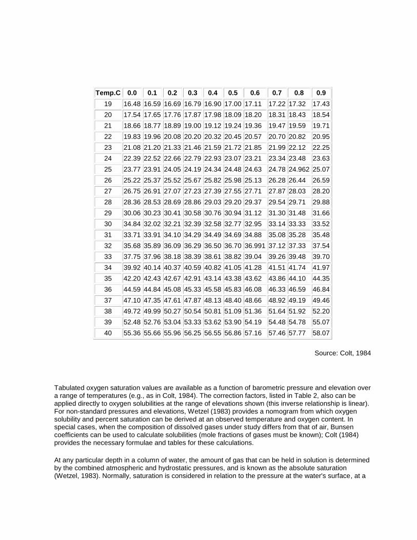
Source: Colt, 1984
Tabulated oxygen saturation values are available as a function of barometric pressure and elevation over a range of temperatures (e.g., as in Colt, 1984). The correction factors, listed in Table 2, also can be applied directly to oxygen solubilities at the range of elevations shown (this inverse relationship is linear). For non-standard pressures and elevations, Wetzel (1983) provides a nomogram from which oxygen solubility and percent saturation can be derived at an observed temperature and oxygen content. In special cases, when the composition of dissolved gases under study differs from that of air, Bunsen coefficients can be used to calculate solubilities (mole fractions of gases must be known); Colt (1984) provides the necessary formulae and tables for these calculations.
At any particular depth in a column of water, the amount of gas that can be held in solution is determined by the combined atmospheric and hydrostatic pressures, and is known as the absolute saturation (Wetzel, 1983). Normally, saturation is considered in relation to the pressure at the water's surface, at a

specific temperature and salinity. Supersaturation, a non-equilibrium situation, is the term used when the partial pressures of gasses (primarily nitrogen and oxygen) in solution exceed their equivalent atmospheric pressures. Hydrostatic pressure increases rapidly with depth and dissolved gas solubility doubles approximately every 10 m (hence, the increased efficiency of aeration devices at depth), while the degree of supersaturation decreases with depth (Colt, 1984). For example, a gas supersaturation of 130 percent (surface measurement) is reduced to 100 percent saturation at a depth of 3.0 m.
Table 2. Correction Factors for Barometric Pressure and Oxygen Saturation at Altitude
ALTITUDE CORRECTION
(feet) (metres) FACTOR
0 0 1.00
500 152 0.98
1000 305 0.96
1500 457 0.95
2000 610 0.93
2500 762 0.91
3000 914 0.89
3500 1067 0.88
4000 1219 0.86
4500 1372 0.84
5000 1524 0.82
5500 1676 0.81
6000 1829 0.80
Notes: 1. Multiply barometric pressure of dissolved oxygen solubility at sea level for the appropriate temperature (Table 3) by the correction factor for your altitude. 2. Interpolate, using linear relationship, for greater accuracy.Source: NCASI, 1985.

Table 3. Solubility of Oxygen in Water (Fresh and Saline) Exposed to Water-saturated Air at Sea Level (760 mm Hg (101.3 kPa)
Oxygen Solubility (mg/L)
Temp. Chlorinity (freshwater)
(C) 0 5.0 10.0 15.0 20.0 25.0
0.0 14.621 13.728 12.888 12.097 11.355 10.657
1.0 14.216 13.356 12.545 11.783 11.066 10.392
2.0 13.829 13.000 12.218 11.483 10.790 10.139
3.0 13.460 12.660 11.906 11.195 10.526 9.897
4.0 13.107 12.335 11.607 10.920 10.273 9.664
5.0 12.770 12.024 11.320 10.656 10.031 9.441
6.0 12.447 11.727 11.046 10.404 9.799 9.228
7.0 12.139 11.442 11.783 10.162 9.576 9.023
8.0 11.843 11.169 10.531 9.930 9.362 8.826
9.0 11.559 10.907 10.290 9.707 9.156 8.636
10.0 11.288 10.656 10.058 9.493 8.959 8.454
11.0 11.027 10.415 9.835 9.287 8.769 8.279
12.0 10.777 10.183 9.621 9.089 8.586 8.111
13.0 10.537 9.961 9.416 8.899 8.411 7.949
14.0 10.306 9.747 9.218 8.716 8.242 7.792
15.0 10.084 9.541 9.027 8.540 8.079 7.642
16.0 9.870 9.344 8.844 8.370 7.922 7.496
17.0 9.665 9.153 8.667 8.207 7.770 7.356
18.0 9.467 8.969 8.497 8.049 7.624 7.221
19.0 9.276 8.792 8.333 7.896 7.483 7.090
20.0 9.092 8.621 8.174 7.749 7.346 6.934
21.0 8.915 8.456 8.021 7.607 7.214 6.842
22.0 8.743 8.297 7.873 7.470 7.087 6.723
23.0 8.578 8.143 7.730 7.337 6.963 6.609
24.0 8.418 7.994 7.591 7.208 6.844 6.498
25.0 8.263 7.850 7.457 7.083 6.728 6.390
26.0 8.113 7.711 7.327 6.962 6.615 6.285
27.0 7.968 7.575 7.201 6.845 6.506 6.184
28.0 7.827 7.444 7.079 6.731 6.400 6.085
29.0 7.691 7.317 6.961 6.621 6.297 5.990
30.0 7.559 7.194 6.845 6.513 6.197 5.896
Notes: 1. Formulae are available for equilibrium oxygen concentration at non-standard pressures and for all chlorinity values. 2. For wastewater, it is necessary to know the ions responsible for the solution's electrical conductivity to correct for their effect on oxygen solubility and use of the tabular value. Source: APHA, 1992

The degree of oxygen supersaturation necessary for bubble growth increases with depth. Ramsey (1962) explained that, in the absence of turbulence, bubbles may form due to the partial pressure of oxygen at depths of less than one metre. Below four metres, oxygen will be maintained in solution by hydrostatic pressure even when extremely supersaturated relative to the pressure at the surface.
The entrainment of air below water falls or dam spillways is a common cause of supersaturation that first came to prominence as an environmental problem in the Pacific Northwest in the Columbia River system (primarily in Washington State, but also below the Hugh Keenleyside Dam near Castlegar). Gas bubbles can develop in fish and invertebrates due to a large imbalance between ambient and internal partial pressures, and lethal or sublethal effects can result. Since oxygen usually is not the principal gas of importance (nitrogen is) and total gas pressure is more central to the issue of supersaturation, gas bubble disease is dealt with in a separate criteria document on total dissolved gases. The effect of hydrostatic pressure also must be taken into account when measuring oxygen concentrations at great depths by an electrode as opposed to a chemical technique. Oxygen solubility remains effectively constant with depth whereas partial pressure increases; therefore, a polarographic probe which measures partial pressure rather than concentration must be corrected accordingly. For example, at 400 m a correction of 5 percent (less) is necessary (Hitchman, 1978).
Turbulence - the diffusion of gas in water is slow and, for equilibrium with atmospheric oxygen to be established, circulation must occur such as in the epilimnion of stratified lakes or at periods of turnover. The rate of oxygen distribution and equilibration is dependent on turbulence. Increased turbulence forms a greater surface area from which excess gasses from supersaturation can dissipate, and brings trapped subsurface water to the surface (NCASI, 1985). In cases where the initial dissolved oxygen concentrations at depth are not far from saturation, equilibrium may occur in a few days. Alternatively, in deep lakes complete oxygenation may never be achieved before thermal stratification terminates circulation for a seasonal interval (Wetzel, 1983). Oxygen distribution will be discussed further in Section 3.1.
Temperature -Temperature, more than any other physical condition in the aquatic environment, affects the solubility potential of dissolved oxygen. This relationship is non-linear as solubility increases considerably in cold water (Wetzel, 1983). Freshwater is saturated with 14.6 mg O2/L at 0 degrees Celsius, which declines to 8.3 mg O2/L at 25 degrees Celsius (at sea level). As solubility declines with increased water temperature, Davis (1975) points out that oxygen partial pressure drops only slightly due to increased molecular activity.
Oxygen solubility tables for a range of temperatures are available from a number of sources; however, references prior to 1981 should be avoided due to updating of these solubilities. Table 3 was extracted from a larger table in APHA (1992) which lists solubility values for dissolved oxygen in freshwater and saline waters, equilibrated with air at one atmosphere (sea level).
Salinity -The oxygen content of water decreases exponentially as salinity increases, such that the difference between solubility in seawater and freshwater is about 20 percent (Wetzel, 1983). Tables (e.g., Table 3) and nomograms (e.g. Figure 1) are available for deriving oxygen saturation in saline waters. The new definition of salinity, which was adopted by the Standard Methods Committee in 1985, is based on the electrical conductivity of seawater. Specific conductance is converted against a known standard (KCl in water) to chlorinity and then to total salinity by a correction factor:
salinity = 1.80655 x chlorinity

The scale has no dimensions, therefore parts per thousand (g/kg) no longer applies (APHA, 1989).
Figure 1. Nomogram of Oxygen Solubility in Air-saturated Water at Different Salinities
Source: Hitchman, 1978
2.2 Analytical Methods
2.2.1 Surface Water
There are two common methods for determining the solubility of oxygen in water: the Winkler or iodometric method and its modifications, and the electrometric method using membrane electrodes. The precision of other chemical and colorimetric methods is invariably less than that for the Winkler method (Hitchman, 1978). The Winkler method involves the more precise titrimetric procedure based on the oxidizing property of dissolved oxygen, while the membrane electrode procedure is based on the rate of diffusion of molecular oxygen across a membrane (APHA, 1992). Since the amount of oxygen in water is dependent upon a complex set of physical properties and biological processes, the method of measurement must be suited to the source water. Temperature, salinity, turbulence, pressure, photosynthetic activity, respiration and chemical interferences (oxidizing or reducing compounds) affect the concentration of dissolved oxygen in water.

Iodometric Procedures - APHA (1992) describes four derivations of the Winkler method, the selection of which is based on minimizing the effects of interfering materials known to be present. For example, the azide modification for most effluent and stream measurements removes interferences caused by nitrite, the most common interference in biologically-treated effluents. Zenon Environmental Laboratories uses this method (reagents include manganese sulphide, potassium salt and sulphuric acid) for calibrating oxygen meters. A determination of 0.05 mg/L is possible, which can ensure a meter accuracy of 0.1 mg/L (Heier, 1991). The other procedures described in APHA (1992) include the permanganate modification used for samples containing ferric and ferrous iron (e.g., acid mine drainage), the alum flocculation modification which removes interferences from high suspended solids, and the copper sulphate-sulfamic acid flocculation modification for biological flocs (e.g., activated sludge) which have high oxygen utilization rates. Further modifications are available for the following: Pomeroy-Kirschman method when high dissolved oxygen levels (> 15 mg/L) or high organic content are present, Alkali-hypochlorite modification in the presence of SO32-, S2 O32-, and polythionate, and the "Short" modification for organic substances which are readily oxidized in strong alkali or by the iodine in acid solution (Hitchman, 1978). A major disadvantage of the above methods is that they are not appropriate for in situ measurements. Samples should be handled carefully to avoid agitation and contact with air, and special equipment is necessary to eliminate changes in pressure and temperature when sampling at depth. It is commonly acknowledged that dissolved oxygen is best measured in the field because of the changes in concentration that are likely to occur between sampling and lab analysis. In some instances, fixative agents (including sulphuric acid, sodium azide) can be used by collectors to stabilize samples for transit to a lab, but these chemicals are costly and extremely corrosive and accuracy of the dissolved oxygen determination still would be questionable. Equipment for measuring oxygen levels in the field is described in the following sections.
Electrometric Procedures - Early oxygen sensors had to be designed for each analytical situation, and electrodes used were subject to direct exposure to the sample medium. The most significant development in the design of efficient sensors was achieved by Dr. Leland Clark whose membrane-covered electrode reduced the risk of contamination and provided a more uniform diffusion layer for oxygen to pass. Present generation meters are a convenient size, simple to operate and reasonably rugged. The submersible electrodes are particularly useful for continuous monitoring, profiling dissolved oxygen with depth and testing waters which have high interference values (effluents, particulates, colour, etc.). Zenon Laboratories, for example, uses an Orion meter for conducting continuous dissolved oxygen analyses for biochemical oxygen demand (Heier, 1991). Some of the newest models incorporate computerized remote control and interfacing to download data (e.g., YSI Model 59). There are three variations of membrane-covered probes commonly in use, each having specific attributes. Figure 2 contains schematic diagrams and probe reactions as examples of galvanic, polarographic and oxygen balance sensors.
The galvanic sensor is self-polarizing and produces its own electric current. A lead or silver anode and a silver cathode reside within a potassium hydroxide electrolyte, and galvanic potential is produced by the reduction of oxygen at the cathode. The current generated is proportional to the rate of oxygen diffusion through the membrane (which is dependent on the concentration of molecular oxygen) (YSI, 1989).
The most common sensor is the polarographic probe, which employs a silver anode and gold cathode in a potassium chloride electrolyte. When voltage is applied, oxygen accepts electrons from the cathode. For each molecule that is reduced, a proportional current is registered that is converted to oxygen content.

A newer and more sophisticated system is employed in oxygen balance sensors, which were designed to address some of the shortcomings of the previous probes. Three electrodes (or more) operate in a potassium hydroxide electrolyte. Oxygen still defuses through a membrane and is reduced at the cathode(s); however, an equal quantity is generated at the anode(s). This diffusion continues until the oxygen tension is balanced on either side of the membrane, and the current necessary to maintain this balance is converted to a read-out of oxygen partial pressure (YSI, 1989).
Figure 2. Oxygen Sensors
Benefits / Drawbacks
- rugged - probe consumes oxygen - high current output facilitates long-term (water flow is necessary) monitoring-electrode is consumed over time - no warm-up required-membrane should be changed periodically
Benefits / Drawbacks
- Teflon membrane is easily-probe consumes oxygen changed in the field water flow is necessary - requires several minutes to equilibrate and give a steady read-out

Benefits / Drawbacks
- fast response-relatively expensive -no electrolyte/electrode consumption-if membrane is fouled or damaged, -membrane may be permanent type sensor must be replaced and -accuracy is not dependent on water flow instrument recalibrated since little if any oxygen is consumed
Source (Figures): YSI, 1989
All of the these sensors are susceptible to various physical conditions which affect the diffusion rate of oxygen through membranes. These influences are (roughly in order of decreasing importance): temperature, water flow, membrane fouling, salinity and barometric pressure. With the exception of contamination, oxygen meters have the compensation circuitry (manual or automatic) necessary to mitigate these influences. Temperature is considered to have the most significant affect on membrane permeability. APHA (1992) recommends that temperature sensitivity be checked regularly against the original calibration. A nomograph for temperature correction is usually supplied with the instrument or one can be constructed. Some meters compensate automatically for temperature using thermistors; however, their accuracy over a wide temperature range has been questionned (APHA, 1992). In YSI probes, the temperature effect on molecular activity causes a three percent change in diffusion rate for every degree Celsius change, even though the oxygen pressure is constant. A temperature-sensitive thermistor corrects this differential. An additional thermistor is usually present to compensate for the varying solubility of oxygen in water when measurements in mg/L are taken (i.e., oxygen content rather than partial pressure or percent saturation). Water flow, such as created by stirring, is particularly important for galvanic and polarographic probes which have oxygen-consumptive reactions that can create a layer of depleted oxygen next to the membrane. These probes are either fitted with stirrers or must be moved through the water column at a minimum specified rate if in static water. Salinity correction also may be necessary to reflect the decline in oxygen carrying capacity with increased salinity. Usually, salinity must be measured by the user and is then manually adjusted on the meter. Finally, instruments may be equipped with automatic barometric pressure compensation, or a tabulated correction factor (Table 2) may be determined and the meter calibrated accordingly after an oxygen reading is taken.
Specific calibration procedures have been developed by manufacturers and it is recommended that these be followed prior to each daily sampling routine. The general rule is to calibrate an oxygen probe under conditions most similar to the water being sampled - preferably in the sample water itself. However, in freshwater containing contaminants, calibration should be done in distilled water. In saltwater, calibration can be done in the water to be tested. Again, if pollutants are present, it is necessary to use clean saltwater or water having the same salt content / specific conductance (can be adjusted by adding potassium chloride). In estuarine water or water with variable ionic content, the sample chlorinity must be determined to allow revision of the original calibration value taken in clear water. Gasses such as hydrogen sulphide, sulphur dioxide and carbon monoxide also will contaminate an oxygen sensor. Membranes should be changed and meters calibrated frequently when the presence of such gasses is suspected (APHA, 1992).
Manufacturers commonly present more than one method of adjusting the oxygen read-out of their meter to a sample of known oxygen content. The following calibration options are described for YSI equipment, but can be considered standard methods for most meters.

Winkler titration - A water sample is subdivided into four parts, three of which are titrated and the results averaged. If one of the values differs from the other two by more than 0.5 mg/L, only the remaining two are averaged. A probe is placed in the fourth sample for three to five minutes to reach thermal equilibrium and then stirred at least 30 seconds before a reading is taken. The reading is adjusted to the titration average. This relatively complex procedure is accurate, but often impractical in the field and is applicable only to freshwater with no interfering ions.
Air-saturated water - A sample of water (usually distilled) is aerated or stirred for approximately 15 minutes to saturation. The water temperature is measured and a solubility table consulted for the appropriate oxygen content (correction for atmospheric pressure or altitude may be necessary). A reading is then taken with the probe and the meter adjusted to the known tabulated value.
Water-saturated air - Air calibration usually is the preferred procedure because of its simplicity and reliability. Air-saturated water and water-saturated air at sea level both have an oxygen partial pressure of 160 mm Hg. However, there is less certainly of the former being 100 percent saturated, while air is by definition air-saturated. To achieve water-saturated air, the probe can be placed in a bottomless container with a wet blotter or a specially made calibration chamber with a few drops of water. YSI's own calibration chamber has a long handle which allows the sealed probe to be incubated underwater to insure proper thermal equilibrium in the field where air/water temperature differentials can be considerable (YSI, 1989).
2.2.2 Interstitial Water
The most long-standing technique for measuring the dissolved oxygen content of sediment water in spawning media has involved the use of standpipes. A standpipe is a length of pointed pipe (usually steel or plastic) that is driven into the bottom sediments. Holes drilled in the lower end accept sub-surface water only, since the top of the pipe projects above the water surface. In 1954, Wickett developed a standpipe apparatus (subsequently referred to as the `Mark I') and procedures for calculating interstitial oxygen content, which have persisted in modified form to the present. His procedure was to drive the sampler to a standard depth (e.g., 30 cm so that the perforations could be at the egg deposition level of 25 cm), pour sand around the pipe to reduce the exchange of surface water next to the pipe, draw off the water within the pipe several times using suction prior to taking a sample, use the Winkler titration method of analysis, and measure the temperature of the pore water. Terhune (1958) developed a `Mark VI' model, primarily to improve the accuracy of measuring permeability using a dye dilution rate technique. He reported consistent results in determining oxygen content within five percent, which he considered satisfactory in view of the natural variability that could be as high as 100 percent in the same redd.
McNeil (1962) focused on improving field measurement accuracy of dissolved oxygen concentration. He described detailed procedures for the fixation and handling of sample water to improve precision, which will not be reproduced here. Two necessary precautions he advised were: 1.) leave the standpipe in the stream for at least 24 hours before sampling to allow conditions to stabilize, and 2.) remove only small water samples (about 30 mL). With respect to the latter, the author showed that variability can be introduced with relatively large withdrawals. If the sub-surface water originated from highly oxygenated stream water at points high in dissolved oxygen, replicate samples had higher readings, wheras lower readings were found for second samples taken at points having low oxygen values due to poorly oxygenated ground water sources. With the development of accurate and reliable dissolved oxygen meters, standpipes also can be used in conjunction with a remote probe (preferably the non-consumptive

type) to avoid the possibility of oxygenating sample water during handling (e.g., as in Woods, 1980). In Sowden and Power's (1985) study of rainbow trout survival in a ground water-fed stream (reported in Section 4.3.2.1), mini-piezometers used for measuring pressure head also functioned as standpipes from which samples were pumped out and analyzed with a polarographic probe. In Scrivener and Brownlee's long-term study of forest harvesting effects on Carnation Creek (1989), interstitial water was simply withdrawn by stainless steel syringe from a depth of 20 cm and analysis done by Hach Kit (reported accuracy of 0.1 mg/L).
In deeper water, the usual standpipe method has obvious limitations. Thompson and Heimer (1967) developed a simple and inexpensive method that utilized a thin (1 cm outside diameter) metal probe perforated at one end and attached to rubber tubing at the other (length adapted to water depth). A 20 cm collar mid-way along the metal tube functioned in similar fashion to that used with the `Mark VI' standpipe, to keep surface flow from travelling down along the outside of the probe. Five millilitre samples were withdrawn through the side of the rubber tubing by syringe and analyzed by a modified micro-Winkler syringe technique. Analyses of dissolved oxygen content in interstitial water in lake and marine sediments are less commonly done and necessarily are more complex. Brinkman et al. (1982) reviewed three existing techniques for collecting pore water (coring, dialysis and direct suction) and identified problems with oxidation, disturbance and suspension of sediments. They decided to design their own apparatus for use in shallow lakes, and their paper details a frame with attached water sampling probe(s) which can be pushed into the sediment. The investigators reported that ambient characteristics were largely maintained, particularly with respect to exclusion of oxidation effects.
3.0 Occurrence in the Environment
3.1 Natural Sources / Depletion
3.1.1 Oxygen Cycles And Distribution
The major sources of dissolved oxygen in water are the atmosphere and photosynthesis by aquatic vegetation (macrophytes and algae). Atmospheric oxygen dissolves in water (and passes out of water) according to the set of physical conditions that were discussed in Section 2. The saturation concentration of dissolved oxygen is quickly achieved at the air-water interface and, in shallow, moving water, will be relatively consistent through the water column. However, since the diffusion of gasses through water is slow, oxygenation of a larger freshwater system with a thermocline barrier is dependent upon water circulation moving aerated water away from the surface (e.g., by wind-induced current, lake turnover and inflows). Gross (1972) explained that the movement of oxygen into marine waters is controlled by some of the same mechanisms, including stratification and biological activity. Saltwater also is oxygenated primarily at the surface. Extensive wind mixing and de-stratification occur in the high latitudes, and the cold, dense waters sink and move into the temperate zones through bottom currents, where they upwell along coasts. In areas of restricted circulation away from these bottom currents, such as in many of British Columbia's inlets, the deep waters remain anoxic (Gross, 1972). In both freshwater and marine systems, oxygen supplied at the surface is steadily diminished with depth according to consumptive demands.
Generally, dissolved oxygen concentrations are in a constant state of flux on a daily basis (consumption/production biotic responses) and seasonal basis (climatic and flow responses). A normal diurnal oxygen cycle would be sinusoidal with a maximum concentration late in the day and minimum in early morning. Distributions of dissolved oxygen at depth, or oxygen profiles, have been studied

intensively in lakes and classified according to lake productivity. While it is not necessary here to examine all identifiable variations in oxygen distribution, it is useful to review some typical situations to clarify the mechanisms which control oxygen content at depth.
At spring turnover, the water column is near 100 percent saturation (12-13 mg /L O2 at 4 degrees Celsius and sea level) for both oligotrophic and eutrophic lakes. There is no temperature/density barrier to internal water circulation mechanisms, and complete mixing is usually possible. With the onset of summer stratification the oxygen profiles diverge. In the idealized oligotrophic lake the oxygen concentration is regulated largely by physical means as stratification occurs. As summer water temperatures increase the dissolved oxygen concentration (and solubility) in the circulating epilimnion decreases. Conversely, a temperature decline in the metalimnion and hypolimnion causes the oxygen concentration to increase and the level of saturation will be close to 100 percent with increasing depth-an orthograde profile. In most oligotrophic situations; however, there still is some organic matter settling into the hypolimnion from the productive zone of the lake and oxidation processes result in undersaturation as stratification progresses (oxygen renewal by circulation and photosynthesis not being possible).
In shallow water, the bulk of the loss attributable to oxidation generally occurs at the sediment/water interface where bacterial activity and organic matter are concentrated. A considerable amount of oxygen also is lost in the water column by bacterial, plant and animal respiration, particularly in deep lakes. Oxygen depletion also occurs by direct chemical oxidation of dissolved organic matter (usually masked by biochemical processes). In eutrophic lakes, hypolimnion depletion may progress to complete anaerobic conditions shortly after summer stratification-a clinograde oxygen profile. Once this happens, there is a shift to anaerobic bacterial metabolism and decomposition processes proceed at a slower rate. The fall turnover of a dimictic lake is brought on by the cooling of epilimnial water with the resultant breakdown of the density barrier at the thermocline and oxygenation of the lower strata. In the winter stratification shown, ice formation in temperate regions prevents the exchange of atmospheric oxygen and the concentration profile for an idealized oligotrophic lake is constant at saturation relative to depth. Again, biotic influences of respiration and oxidation are normally present and there is a reduction in oxygen concentration with depth. In eutrophic lakes, the photic zone is reduced but can remain active where sufficient light penetration through ice continues and the normal consumptive demands are lessened by cooler temperatures. The resultant oxygen profile showing depletion at depth is similar to, but more gradual than for summer stratification (Wetzel, 1983).
One common variation of the oxygen profiles involves an increase in metalimnetic oxygen and is termed a positive heterograde curve. Typically, dissolved oxygen solubility in the epilimnion decreases with increasing summer temperature and oxidative consumption in the hypolimnion results in a clinograde curve. This leaves the highest oxygen concentrations (saturation or higher) in the metalimnion. When algal communities adapted to this strata (e.g., blue-greens) are active, supersaturation of several hundred percent can result. Rooted aquatic vegetation in the lower littoral zone also can enrich this zone. The actual depth of this maxima is dependent on water transparency and is usually in the 3 to 10 m range. Metalimnetic oxygen maxima tend to be more pronounced in relatively deep lakes that are well stratified; the bottom profiles are such that a small proportion of the sediments (site of highest bacterial utilization of oxygen) are in contact with the metalimnion. A metalimnetic oxygen minimum (or negative heterograde curve) is more uncommon and can result from a variety of reasons: 1) oxidizable material produced within or outside the catch-basin is continuously decomposed while it sinks; when it encounters the dense metalimnetic water it slows down and exacts a proportionately greater oxygen demand in this zone, 2) respiratory demand from large concentrations of zooplankton, and 3) in cases where a gradual

bottom slope (site of high oxygen utilization) coincides with the prevailing metalimnion, horizontal mixing (greater in the zone) can spread the reduction laterally.
There are other important mechanisms that control oxygen levels in the littoral zone, which can be quite different to that of the pelagic zone. For example, well developed stands of aquatic macrophytes and associated periphyton will substantially raise oxygen levels during photosynthesis and consume oxygen during respiration at night. This diurnal event also gives rise to a diel cycle due to the net production of oxygen during the growth seasons. Late in the year, much of the macrophyte standing crop dies back to the root crown and the concomitant decomposition can cause a prolonged oxygen demand extending beyond the littoral areas. Understandably, the proportion of littoral development ultimately determines the magnitude of these influences. Frodge et al. (1990) observed that where this proportion was very high, the dissolved oxygen profile can be radically different over short distances. The horizontal distribution of dissolved oxygen in two shallow Washington lakes was associated with the patchy distribution of aquatic plants. Open water, being well-mixed in comparison to vegetated areas, had higher sub-surface oxygen concentrations than beneath either submergent or floating plant canopies. Plant morphology largely determined the differences in vertical oxygen profiles and diurnal changes (if any). For submersed plants such as Myriophyllum sibiricum and Ceratophyllum demersum, dissolved oxygen concentrations within and immediately below the canopies were regularly at supersaturation (>30 mg/L) during daytime, but declined rapidly to consistently low levels when the effects of wind and sunlight were cut-off. In a typical western Washington lake dominated by Brasenia schreberi, the floating leaves isolated the entire water column even further and dissolved oxygen levels of 2 mg/L or less were recorded, with little recovery during daylight. Brasenia schreberi and other floating-leaved macrophytes are able to exchange gasses directly with the atmosphere and make no substantial oxygen contribution to the water column (Frodge et al. 1990). Profuse phytoplankton growth in very eutrophic lakes also will produce diel fluctuations, and if die-off occurs rapidly (e.g., when snow-covered ice blocks photosynthesis) dissolved oxygen may be completely exhausted (Wetzel, 1983).
Similar consumptive processes, which surpass the resupply of oxygen, exist in coastal marine areas and are often exaggerated by very high water temperatures (lowered oxygen solubility) and organic effluents from anthropogenic sources. The odorous hydrogen sulphide present at low tide in coastal marshes is an indicator of anaerobic metabolism (Gross, 1972).
3.1.2 Oxygen Pathways
There is a plethora of complex pathways involving oxygen production and utilization in water, the specifics of which are not a primary concern here. However, brief descriptions are given of some of the more important redox processes.
Other than atmospheric input, the principal source of dissolved oxygen in the surface strata is photosynthesis. Phytoplankton and attached vegetation also represent a major (often predominant) supply of new organic matter. The simplified photosynthetic reaction is summarized:
6 CO2 + 12 H2O --------->C6 H12 O6 + 6 H2O + 6 O2 (Wetzel, 1983)
This reaction is mediated by a light pigment receptor

There is a transfer of carbon to carbohydrate and water is oxidized to oxygen. This release of oxygen in the photic zone commonly gives rise to slight supersaturation. In very rare instances, photosynthetic oxygen supersaturation has caused mortality in freshwater and marine fishes (NCASI, 1985).
Photosynthesis produces reduced states of free energy and non-equilibrium concentrations of oxygen, carbon, nitrogen and sulphur compounds. Respiratory, fermentative and other reactions which bacteria mediate, act to restore this equilibrium. This is accomplished by specific bacteria decomposing the thermodynamically unstable products of photosynthesis and thereby obtaining a source of energy for their metabolic demands. In large, deep lakes most bacterial respiration may occur in the water column, whereas in shallower water bodies with high organic inputs from allochthonous sources (shoreline vegetation), benthic decomposition may dominate. When oxidative respiratory processes in the lower strata outpace the supply of oxygen, anaerobic metabolism proceeds using substitution (oxidative) compounds. However, the oxidizable byproducts which evolve (e.g., methane, hydrogen, hydrogen sulphide, carbon monoxide) are released to the overlying oxic waters and further reduce oxygen content in the system. In water, the principal reactants in redox processes are limited to carbon, oxygen, nitrogen, sulphur, iron and manganese. Some characteristic reactions involving dissolved oxygen (hydrogen ion acceptor) in oxygen-consuming redox reactions are listed below (from Wetzel, 1983):
(Iron) FeS2 + 31/2 O2 + H2O --------> FeSO4 + H2SO4 2 FeSO4 + 1/2 O2 + H2SO4 ----------> Fe2 (SO4)3 + H2O (in acid mine drainage where pH<3) 4 FeCO3 + O2 + 6 H2O ----------> 4 Fe (OH)3 + 4 CO2
(Manganese) 4 MnCO3 + O2 -----------> 2 Mn2O3 + 4 CO2 Mn
2+ + 1/2 O2 + H2O -----------> MnO2 + 2 H
+
(Sulphur) S + 11/2 O2 + H2O ----------> H2SO4 H2S + 1/2 O2 ----------> S
0 + H2O (and see iron above)
(Nitrogen-Nitrification) NH4+ + 2 O2 --------> NO3
- + H2O + 2 H
+ (overall reaction)
(Methane) 5 CH4 + 8 O2 ---------> 2 (CH2O) + 3 CO2 + 8 H2O
(Carbon Monoxide) CO + 1/2 O2 ---------> CO2
3.2 Anthropogenic Sources / Depletion
As discussed in the previous section, the dissolved oxygen content of water is largely controlled by the balance between input and consumptive metabolism (of oxidizable matter received). Anthropogenic influences (industrial-including deforestation, agricultural and municipal wastes) tend to load the latter scale by the addition of organic effluents. The depletion of dissolved oxygen in receiving waters is often a ready indicator of wastewater treatment requirements, and specific empirical procedures have been devised to measure oxygen demand. Biochemical oxygen demand (BOD) is a standard microbial incubation procedure that measures the oxygen required to oxidize organic material and certain inorganic materials (e.g., sulphides and ferrous iron) over a given time period (usually five days). Alternately, the measure for the amount of oxygen required to chemically oxidize reduced minerals and organic matter of a sample is termed chemical oxygen demand (COD). Both terms are applied to the

level of reducing material present from a combination of natural and anthropogenic sources and have particular usefulness in assessing the potential impacts of effluents. Provincial waste discharge permits normally prescribe an allowable quantity of BOD according to the volume of effluent and consideration of the type of receiving water. Few ambient guidelines exist for BOD/COD values and none are proposed; however, McNeeley et al. (1979) consider waters with BOD5 levels greater than 10 mg/L to be polluted and less than 4 mg/L to be reasonably clean.
Wastes that are primarily nutrient related and/or high in carbon may enhance or deplete dissolved oxygen levels and commonly do both depending on the location in the water column. Additional oxygen is usually produced in the photic zone by increased primary production following enhancement by inorganic nitrogen and phosphorus, but a subsequent drop in the nutrient supply can be accompanied by algal die-off, decomposition and oxygen depletion. Gross (1972) describes a secondary effect (negative) from a nutrient-enhanced regime in a coastal environment, which allows blue-green algae to replace diatoms as the dominant growth. Local zooplankton are not able to utilize the algae, which then sink and enter the decomposing cycle rather than the grazing food chain. Ultimately, the depletion of deep water oxygen exceeds the rate of replenishment from bottom currents, anoxia develops and benthic organisms die.
In British Columbia, some of the best illustrations of the profound influences that effluent can have on dissolved oxygen in fresh and marine waters come from the pulp and paper industry (bleached kraft and sulphite mill effluents in particular). In some of these cases, the resultant oxygen deficiency in receiving waters is the most critical environmental hazard. Inlets which characteristically have poor water exchange and naturally depressed oxygen levels are vulnerable, as the assimilative capacity for high BOD discharges may be minimal. Examples of this can be found in Kay's (1986) review of coastal water quality, which reported serious dissolved oxygen deficiencies associated with kraft and sulphite pulping mills located at Alberni Inlet, Neuroutsos Inlet, Cousins Inlet and Porpoise Harbour/Wainwright Basin. The Port Alberni case, where a mill outfall is located at the head of an inlet adjacent to a freshwater inflow (Somass River), is typical of the processes which can affect the oxygen budget. The inlet is highly stratified by a halocline layer, which varies between depths of 2 to 5 m, separating freshwater and seawater (a natural barrier against the introduction of atmospheric oxygen). The initial period of discharge (1949-1956) directly to the harbour resulted in chronic oxygen depression below the halocline due to the high BOD of dissolved kraft mill effluents (lignin, carbohydrates, organic acids, alcohols) and decomposition of solid organic material on the bottom. Effluent was diverted to the mouth of the Somass River in 1956 to allow diffusion into the more oxygen-saturated surface layer; however, low oxygen levels persisted above and below the halocline. Parker and Sibert (1972) suggested that a secondary effect of pulping wastes on oxygen levels was caused by the humic colour, which attenuated light penetration within the photic zone and inhibited photosynthesis/oxygen production. Since 1970, effluents at Port Alberni have been aerated and clarified to reduce BOD and colour, and discharges have been varied to correspond with flow in the Somass River. Unfortunately, most of the improvement in dissolved oxygen concentration has been confined to water above the halocline (Kay, 1986; Parker and Sibert, 1972).
Aeration of effluent from pulp and paper mills and municipal biological treatment lagoons is common practice, and in some cases oxygen is introduced to bring concentrations closer to that of the receiving water. Such applications of pure oxygen have demonstrated efficiency and its further use within the forest products industry is being considered (NCASI, 1985). A potential hazard with oxygenation is that supersaturation can occur and mitigation procedures may be necessary. Thermal effluents discharged to saturated water also can cause supersaturation, since heating actually reduces oxygen-carrying capacity.

Manipulation of oxygen levels is used in fish hatcheries to increase the carrying capacity for high fish densities. Similarly, in lakes which stratify, it is possible to increase the area habitable by fish through increasing oxygen levels in the lower strata. Hypolimetic aeration can reduce fish kills in summer and improve the benthic food supply. Either air or pure oxygen (to improve efficiency) is injected at depth without destratifying the water column. A review of 13 lake aerators by Cook et al. (1986) found that all but one increased the level of hypolimetic oxygen to at least 7 mg/L. Oxygenation of the hypolimnion can be accomplished in other ways. Artificial circulation by injecting compressed air can serve to move deoxygenated water to the surface and allow equalization with the atmosphere (rather than provide oxygen by diffusion from the injected air).
The difference from hypolimnetic aeration is that the entire water column is mixed and water temperature is increased at depth. Hypolimnetic withdrawals from reservoirs can be used to provide downstream cooling in summer,with a side benefit being the shortened detention time of the lower strata water with less likelihood of anoxic conditions developing.
Reduction of dissolved oxygen by mariculture net-pens is not as common as in freshwater facilities because of the obvious differences in waste assimilation capacity. Usually, the majority of the oxygen demand originates from feed and feces which accumulate below net-pens, and the effects tend to be localized and transient. Weston (1986) reported that one and one-half to three times as much oxygen may go to decomposition processes as to fish respiration. In what was considered a worst-case situation, some decrease in dissolved oxygen in and around net-pens was found in a poorly flushed area in Henderson Inlet, Puget Sound. The effect was limited to periods of summer stratification when surface and bottom current velocities were extremely low. Most studies of water quality around fish farms in British Columbia (particularly Sechelt Inlet) and Washington State have shown mariculture to have a negligible effect on dissolved oxygen levels (Weston, 1986).
3.3 Natural Levels In Water And Sediment
3.3.1 Freshwater
The concentration range of dissolved oxygen in western Canadian surface waters, documented between 1980 and 1985, was from non-detectable to 18.4 mg/L (NAQUADAT, 1985). In British Columbia surface waters, dissolved oxygen levels are generally high (greater than 10 mg/L) and close to saturation. Even in the lower Fraser River, where effluent discharges are most numerous, median dissolved oxygen concentration from 1970 to 1978 were above 9.5 mg/L (10th percentiles exceeded 7.0 mg/L) with saturations mainly between 80 and 100 percent (Drinnan and Clark, 1980). Below the major sewage treatment plant outfall at Annacis Island, the dissolved oxygen concentration showed a decrease of less than 1 mg/L in the effluent plume, but levels returned to normal downstream. In the main river channel, levels were similar to the median of 10.8 mg/L oxygen for most streams in British Columbia (Drinnan and Clark, 1980).
At townsites in the upper Fraser River watershed, the assimilative capacity (flow) in the river and its tributaries is reduced, and localized decreases in dissolved oxygen are more pronounced. For example, mean dissolved oxygen levels in the Nechako River, near effluent discharges at Fort Fraser and Vanderhoof, have been reported as low as 4.7 mg/L (ENVIROCON, 1981). In the heavily impounded Columbia River mainstem, dissolved oxygen levels rarely fall below 8 mg/L. However, some of the

tributaries which experience low flows and elevated summer temperatures may contain less than 6 mg/L oxygen (Stober and Nakatani, 1992).
As discussed in Section 3.1.1, oxygen regimes in lakes are dependent primarily upon seasonal temperature variation, depth and trophic status. The Okanagan Valley is a major British Columbia waterway that contains a number of lakes which illustrate the variability in oxygen content relative to morphometry and productivity. A study for the Canada-British Columbia Okanagan Basin Agreement (1974) determined: epilimnial oxygen concentrations remained near saturation in all lakes through the summer, the hypolimnia of Osoyoos, Wood and Skaha Lakes were below saturation for the same period, and the hypolimnia of Kalamalka and Wood Lake remained well oxygenated. Based on a trophic index correlated with the oxygen depletion of hypolimnetic water during summer stratification, the lakes were classified as: Kalamalka and Okanagan Lakes-oligotrophic, Osoyoos Lake-mesotrophic and Skaha and Wood Lakes-eutrophic (Canada BCOBA, 1974). Kalamalka Lake exhibits an `orthograde' oxygen profile during summer stratification, while the shallow, productive water column of Wood Lake produces a `clinograde' profile. The latter progresses to a `positive heterograde' profile in mid-summer, whereby an improvement in water clarity maximizes algal production at the thermocline. Supersaturated oxygen levels (up to 135 percent) maintained by the hydrostatic pressure at 10 m have been observed (Anon, 1974). An example of a `negative heterograde' curve, was taken from Skaha Lake in October, 1979 (Jensen, 1981). Since the study, dissolved oxygen concentrations at Wood Lake have been improving (Bryan, 1990).
3.3.2 Marine
The quantity of oxygen dissolved in seawater is less (by about 20 percent) than in lower density freshwater at a given temperature and pressure. For example, at a salinity of 27 g/kg (now referred to as a chlorinity of 15-as per Section 2.1), oxygen solubility ranges from 12.1 mg/L at 0 degrees Celsius to 7.1 mg/L at 25 degrees Celsius (compared to freshwater solubilities of 14.6 and 8.3 mg/L respectively, from Table 1). Surface waters usually are at or near equilibrium with atmospheric oxygen, while supersaturation is common in the first few tens of metres (photic zone). This surface-supplied oxygen is diminished by consumptive demands in the upper several hundred metres and, in the deep ocean where these demands are limited, oxygen concentrations are relatively uniform but well below saturation (Gross, 1972).
Coastal waters have much more variable water quality and are commonly the site of major anthropogenic activity and important biological production. Most of British Columbia's open coast tends to be well-mixed through upwelling, tidal currents and wind forces and consequently is well-oxygenated. In the more protected inside passages, dissolved oxygen values are extremely variable and depend largely on the accessibility of deep water inflow to replace oxygen depleted by biological processes. Thompson (1981) explained that the dilution of Strait of Georgia water by Fraser River runoff and the seaward migration of this brackish surface layer, particularly through the southern passes, results in an inflow of oceanic water through the Strait of Juan de Fuca. This flushing action maintains the present oxygen regime of the strait. Replacement time for surface water (less than 30 m) is only one month. A 60 m deep sill between Victoria and Port Angeles presents a partial blockage to the Pacific inflow; however, oxygen-rich water still is able to penetrate to the deeper basins of the Strait of Georgia and complete renewal can occur within a year. The variability of the source water quality also has considerable influence. Upwelling along the outer coast is most prevalent in mid-summer, hence dissolved oxygen levels in the Strait of Juan de Fuca are lowered. Added to the accelerated biological-related consumption during this period in sub-surface waters, oxygen levels in the Strait of Georgia reach minimum levels by

early Autum. Conversely, relatively oxygen-rich water moves into the southern straits during the winter/spring months. Numerous sills also are in evidence in the northern passage along Queen Charlotte Strait, Broughton Strait, Johnstone Strait and Discovery Passage. Some layering of the waters in Queen Charlotte Strait occurs as the well-oxygenated surface water moves seaward and the stratified ocean water moves inland. Dissolved oxygen levels at the bottom of the basin remain above 4.5 mg/L. Active tidal currents coupled with the movement of water over the irregular bottom topography keep the remainder of the northern passage well-mixed and oxygen levels uniform from top to bottom year-round. Thompson's (1981) September, 1977 profile taken mid-channel from Broughton Strait to Discovery Passage shows a range of only 5.1 to 6.6 mg O2/L.
The British Columbia coast is further characterized by its numerous inlets, many of which are the site of intense commercial activity. Oft-cited works by Pickard (1961; 1963) on the physical and chemical features of prominent inlets along Vancouver Island and the mainland are still useful summaries. He found that oxygen saturation values generally increased slightly with depth in the low salinity surface layers due to the drop in temperature and, below the brackish water (halocline), dropped by about 10 percent with the rise in salinity. Oxygen maxima at the head of an inlet were the result of river inflows, while maxima at the mouth were most often cases of phytoplankton causing supersaturation (110 to 130 percent). In the latter situation, these maxima were at the 3 to 8 m depth where phytoplankton were most concentrated. In deep water, oxygen values declined to 35 to 60 percent saturation (3.8-5.7 mg/L); minimum oxygen levels were sometimes homogeneous from a depth of 200 to 300 m, to the bottom. Pickard (1961) also found mid-depth maxima and explained that the frequent inflows of oxygenated, higher salinity water over the sills near the entrance of inlets (to replace net surface out-flow) displaced oxygen-deficient water upwards. This water mass was then held at mid-depth below the less dense surface layers.
Such occurrences were more typical of low-runoff inlets (e.g., Sechelt) where induced estuarine circulation was not sufficient to replace oxygen. Low-runoff inlets, as typified by those on Vancouver Island, tended to show greater variability of dissolved oxygen than large-runoff inlets. Shallow sills were considered important in limiting deep water circulation, and less internal runoff (than mainland inlets) contributed to lower oxygen levels. Below 100 m, dissolved oxygen was usually less than 5.7 mg/L, in many cases was less than 1.4 mg/L and in a few sites within the inner basins of Tofino, Nitinat and Saanich inlets, values of Ong/L were recorded (Pickard, 1963). In Saanich Inlet (24 km long and 230 m deep) which receives low runoff and has a shallow sill at 75 m, only the water above this level is well-mixed. A thermocline usually develops in summer at 5 to 10 m and the deep waters become anoxic. Oxygen is replenished once a year by the inflow of water over the sill from the Strait of Georgia, although this supply can be depleted in a few months (Harrison et al. 1983).
3.3.3 Stream Sediment
Interstitial or sediment oxygen concentrations are highly variable and can differ markedly from the overlying water due to a number of independent variables which include: surface and interstitial water velocity/discharge, hydraulic gradient, sediment texture and porosity, bottom morphology, daily water temperature fluctuation and the consumptive oxygen demand of the substrate. In standing water environments, interactions between the diverse sediment biota and the concentration of particulate organic material are the major cause of oxygen depletion (both through respiration and release of decomposition byproducts in reduced form). As discussed earlier, oxygen itself will regulate important redox reactions at the sediment/water interface. Oxygen penetration into the substrate from the water column is governed by the rate of turbulence of superficial sediments and by the oxygen demand per unit

volume; typically, diffusion from even well-aerated water will only supply the top few centimetres (Wetzel, 1983). In some cases, filter feeding organisms can introduce oxygen to greater depths by physically reworking compacted, oxygen-deficient mud and extending the habitable range. Similarly, in riverine environments, the act of redd construction by salmonids through excavation and backfilling results in localized dispersal of fine sediments and increased interstitial flows for improved oxygen delivery to the buried eggs. The following discussion is confined to stream sediment oxygen levels in spawning habitat.
Koski (1965) found relatively high oxygen levels (close to saturation) in his examination of 31 coho salmon redds in three small costal streams in Oregon. The variability of his measurements was high, both between redds (mean values of 3.0 to 11.8 mg O2/L) and within redds (up to 6 mg O2/L at a given time). Mean minimum interstitial oxygen concentrations for the three streams were 7.4, 7.5 and 8.7 mg O2/L, which represented reductions of 3.2, 3.5 and 1.4 mg O2/L respectively, from surface water values (at or near saturation). Hollender (1981) also encountered high variability both spatially and temporally in his study of dissolved oxygen in brook trout redds in two Pennsylvania streams. Stream and interstitial water temperatures were almost identical and followed the same temporal pattern. The overall mean dissolved oxygen levels in natural redds was 8.2 mg/L, within a range of means between 3.7 and 11.6 mg/L. Only about one-quarter of the redds had mean oxygen levels below 6 mg/L. The interstitial concentrations were lower, but closely followed those of the surface water which averaged more than 10 mg/L. In one stream, the substrate/surface water differential was 2.1 and 2.8 mg O2/L in consecutive years, and in the second stream was 3.7 mg O2/L for one year. Surprisingly, the corresponding geometric mean particle sizes within redds were 2.5, 3.0 and 4.4 mm, respectively (an inverse relationship with dissolved oxygen). On the strength of the two previously cited studies on natural redds, the US EPA (1986) suggested that interstitial oxygen be considered to be at least 3 mg/L lower than that of the overlying water as a result of the reduced permeability and consumptive demands in that region. Field data collected by Pyper and Vernon (1955) suggested that the mean dissolved oxygen in interstitial water of a typical sockeye spawning stream in British Columbia would be about 75 percent of saturation. Sowden and Power (1985) examined rainbow trout redds in an Ontario stream which had been subjected to moderate sedimentation from agricultural land. Ground water upwelling appeared to control the dissolved oxygen content of the redds, although concentrations were variable. The average mean oxygen level for 19 redds was 5.5 mg/L (range of mean values was 2.0 to 8.9 mg/L). Unfortunately, no surface water oxygen concentrations were collected for comparison.
Other researchers have reported levels of dissolved oxygen in simulated redds, in which eggs are buried manually. Coble (1961) noted that interstitial oxygen content in two Oregon streams was closely correlated with sub-surface water velocity and measured a reduction of about 5 mg/L in artificial redds relative to the overlying water (interstitial oxygen averaged 6 mg/L). Similarly, McLean (1988) described the results of siltation on artificial spawning media in the Little Qualicum River and found that interstitial oxygen was positively correlated with substrate permeability. Dissolved oxygen levels in silted channel sections varied between 0.5 and 9.3 mg/L (5.4 mg/L approximate average), and after intensive cleaning all interstitial oxygen levels were above 9.5 mg/L. Turnpenny and Williams (1980) recorded interstitial dissolved oxygen concentrations in artificial rainbow trout redds of between 8 and 11.4 mg/L (80-103% of saturation), which were relatively high considering the industrial influences at some of their study sites. At two control sites, away from potential impacts, the maximum differential between surface water (saturation) and interstitial water over a 28-day incubation period was 2 to 3 mg/L. Chevalier and Murphy (1985) reported oxygen levels within simulated redds along the Tucannon River, Washington. Between February and June, 1980 (period of salmon egg incubation), the differential between average mean surface oxygen saturation and interstitial water at five sites was 3.4 mg/L; however, the range of mean values was considerable (0.19 mg/L to 7.71 mg/L). Low oxygen levels in the lower reaches reflected the presence of organic matter and high sediment oxygen demand. During a second period in May, 1981,

the relationship between sediment organics and oxygen levels was less obvious, although the mean surface/sub-surface differential was similar at 3.75 mg/L (surface saturations were 10.53 to 11.83 mg/L, while interstitial concentrations varied from 3.58 to 11.26 mg/L). The investigations of artificial redds by Turnpenny and Williams (1980) and Chevalier and Murphy (1985) support the US EPA's assumption (based on natural redds) that a differential on the order of 3 mg/L exists between the interstitial environment and the water column.
Except in cases of upwelling ground water, the oxygen content of interstitial water is highly dependent on flow driven by the overlying hydraulic gradient. Bed composition and particle size play a major regulatory role in the extent of this downwelling. Understandably, substrates predominated by fines have more limited exchange with surface water for oxygen replenishment. Whitman and Clark (1982) found that restricted porosity resulted in considerable variation between surface and sediment water oxygen in a Texas stream. Along a homogeneous, sandy riffle there was a reduction (from overlying water) of approximately 5.5 mg O2/L at a sediment depth of 10 cm and interstitial oxygen averaged about 3.5 mg/L. The level of fine particles (clay, silt, sand) can become critical in salmonid spawning gravels.
Some of the most detailed work on the deposition of fine particles and resultant impairment of fish production has been done in the Pacific Northwest. The Tucannon River study in southeastern Washington was primarily concerned with fish habitat loss attributable to agricultural practices. Chevalier and Carson (1985) investigated the intricate relationship between sediment fraction size and flow mechanics of this river and derived an interstitial dissolved oxygen transfer model for use in predicting salmonid embryo survival. The hydraulic impairment by fine particles appears to become critical to egg survival when the sand fraction approaches 20 to 25 percent by volume or when silt / clay / fraction reaches only one to two percent by volume. A small amount of silt was found to be particularly effective at blocking interstitial flow if the fine particles were arranged in layers and not evenly dispersed (often the case in the Tucannon River). Through modelling parameters which approximated natural conditions of the river, the researchers showed that vertical and horizontal diffusion of oxygen was insignificant below the top 8 cm of substrate materials relative to convective transport of oxygen by horizontal flow. However, as pore spaces became plugged, velocity decreased to the point where diffusion became the only source of oxygen supply.
In British Columbia, a long term study on the effects of logging on salmonid spawning habitat was conducted at Carnation Creek on Vancouver Island. Scrivener and Brownlee (1980) determined that prior to the effects of major siltation (pre-1978) the mean interstitial oxygen concentrations had followed seasonal trends relative to surface concentrations: pre-spawning period was 5.4 mg/L, post-spawning period was 6.3 mg/L and pre-emergence period was 6.6 mg/L, at a mean saturation potential of 12.6 mg/L. Subsequent declines in dissolved oxygen were attributed to increased consumption from greater loadings of organics and a decrease in gravel permeability due to infilling by fine sediments. Through 1980, interstitial oxygen concentrations ranged between 0.5 and 11.4 mg/L. In August, 1982, interstitial oxygen concentrations ranged from 1.3 to 8.9 mg/L while surface concentrations were 7.5 to 9.5 mg/L. The researchers noted that gravel size could not account for more than 20 percent of the variability in dissolved oxygen and a positive correlation with mean particle size was only apparent in the top 15 cm layer. Interstitial oxygen varied between 18 and 96 % of surface levels when the geometric mean particle size was 10 to 12 mm, but was always greater than 60 % when particle size was more than 18 mm (Figure 3). While other influences (flow and direction, hydraulic gradient, micro-topography, consumptive demand) obviously were strong, it was suggested that a better correlation may have been obtained at times other than during summer minimum flows (Scrivener and Brownlee, 1989). Most of the study sites probably had adequate oxygen for normal development prior to 1978 (pre-logging) when post-spawning interstial oxygen levels were normally distributed about a mean concentration of 6.3 mg/L. After logging,
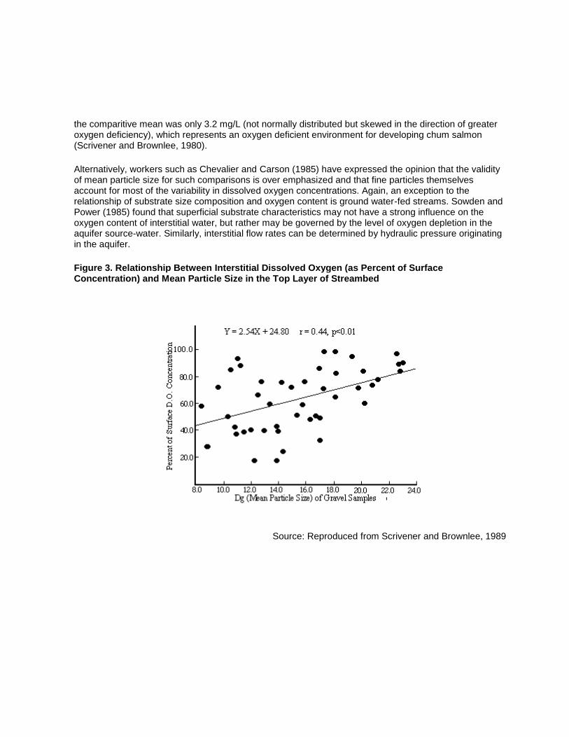
the comparitive mean was only 3.2 mg/L (not normally distributed but skewed in the direction of greater oxygen deficiency), which represents an oxygen deficient environment for developing chum salmon (Scrivener and Brownlee, 1980).
Alternatively, workers such as Chevalier and Carson (1985) have expressed the opinion that the validity of mean particle size for such comparisons is over emphasized and that fine particles themselves account for most of the variability in dissolved oxygen concentrations. Again, an exception to the relationship of substrate size composition and oxygen content is ground water-fed streams. Sowden and Power (1985) found that superficial substrate characteristics may not have a strong influence on the oxygen content of interstitial water, but rather may be governed by the level of oxygen depletion in the aquifer source-water. Similarly, interstitial flow rates can be determined by hydraulic pressure originating in the aquifer.
Figure 3. Relationship Between Interstitial Dissolved Oxygen (as Percent of Surface Concentration) and Mean Particle Size in the Top Layer of Streambed
Source: Reproduced from Scrivener and Brownlee, 1989

4.0 Aquatic Life (Freshwater, Marine and Sediment)
4.1 Effects On Algae And Macrophytes
The more familiar effects of dissolved oxygen on primary producers are indirect and are beyond the scope of this discussion (e.g., as in the well-documented role of oxygen in nutrient availability). Since algae and macrophytes are net producers of oxygen and located in relatively close proximity to the surface they are not usually associated with exceptionally undersaturated water. Dissolved oxygen is required for respiration, but generally will not be as limiting as some other condition such as light or hydrostatic pressure.
One of the physiological obstacles to the evolutionary transition of plants (primarily terrestrial origins) into freshwater was the relative lack of oxygen-0.8 percent in water by volume as compared to 20 percent in air-and slower diffusion rates of gasses in water. During darkness, dissolved oxygen is the most critical factor influencing the respiration of submersed macrophytes. The diurnal photosynthetic cycle produces oxygen which is used immediately for respiration and the excess can be stored in internal air spaces or lacunae for use in early morning when the supply may become low. Research suggests that with decreasing dissolved oxygen there is a logarithmic decrease in the rate of respiration in many freshwater species and a proportionate decrease in the rate of respiration in marine angiosperms and algae (Sculthorpe, 1967). Oxygen dependence has been demonstrated in plants when the internal oxygen supply becomes exhausted (the rate of oxygen diffusion from the surrounding water then becomes limiting).
Since aquatic plants are often rooted in anaerobic sediments they have had to devise several adaptations. Depending on the species, rhizomes of freshwater plants are either supplied oxygen from the foliage or, in those perennials that overwinter in a dormant condition, must utilize the Kreb's cycle (energy release through anaerobic glycolysis and fermentation) for respiration in the absence of oxygen. The lacunae may be continuous from the roots to the above water structures, thereby allowing very efficient gas transport. Where the lacunae are isolated by plates of cells, these pockets may store and prevent loss of photosynthetically produced oxygen from submerged plants. An example of a biochemical adaptation is the production of respiratory cytochromes which have an unusually high affinity for oxygen (Moss, 1980).
Lewin (1962) reported that aerobic respiration in some algae has been found to continue unimpaired at very low oxygen tensions. Under anaerobic conditions most plants start to ferment (breakdown carbohydrate to produce carbon dioxide, ethanol and organic acids). A few highly specialized algal species in several classes are capable of anaerobic metabolism; however, there has been no evidence of anaerobic, heterotrophic growth as found in biochemically similar species of bacteria. The development of anaerobic conditions may select against perennation (overwintering adaptations) of oligotrophic phytoplankton, but is tolerated by the dormant life stages of many eutrophic species (may be conducive to the seasonal growth of Microcystis [Reynolds, 1984]).
4.2 Effects on Invertebrates
The specific oxygen requirements of aquatic invertebrates have been studied extensively and the great range of tolerances identified is predictable for such a diverse group. Davis (1975) explained that organisms which are most able to tolerate low oxygen conditions are capable of some form of anaerobic

metabolism. This enables some normally aerobic invertebrates to inhabit low oxygen environments for extended periods, while others may be able to tolerate only a brief oxygen debt (due to accumulated metabolic products which must be oxidized). Animals with high metabolic rates are typically less tolerant of reduced oxygen than sluggish forms (e.g., early life stages or behaviourally inactive forms). Many invertebrates can regulate oxygen uptake over a range of oxygen tension (are oxygen-independent), while in others, oxygen uptake conforms to availability (are oxygen-dependent). Davis (1975) summarized a considerable body of literature for many freshwater and marine organisms and concluded that knowledge of chronic effects and community oxygen requirements was not sufficient to establish safe criteria. However, it is useful to review some of his material and other works to determine the sensitivities of representative local taxa.
4.2.1 Freshwater
Oxygen sensitivities of freshwater invertebrates commonly reflect the habitats in which they live. In aquatic environments, the respiratory rate usually will depend on the oxygen concentration, and this rate may decline sharply at low-to mid-saturation levels. Currents can be an important factor as the oxygen concentration tolerated by some animals at times is decreased with increased flow. Stream organisms which depend on currents for replenishment of oxygen have comparatively slow body and gill movements (Moss, 1980). Oxygen dependence/ independence are spread through most of the major invertebrate groups and sensitivities are varied, thus generalizations are difficult. A summary of responses to low oxygen is presented in Table 4.
Table 4. Oxygen Sensitivites of some Freshwater Invertebrates
1
CLASSIFICATION2 HABITAT
(where specified or known)
RESPONSE TO LOW OXYGEN
(mg O2/L)
REFERENCE
Annelida: (leech) Erpobdella testacea
(varied) -regulated oxygen uptake and lowered its Pc (critical O2tension) following acclimation to low oxygen
Davis, 1975
Gastropoda: (snails) most littoral snails
-oxygen dependent, as respiratory rate falls progressively with oxygen content
Moss, 1980
Lymnaeidae, Physidae -withstood 6 h of anaerobiosis Davis, 1975
Planorbidae and operculates
-withstood 24 h of anaerobiosis
Ancylus fluviatilus -climbed to the water's surface when dissolved oxygen declined
Acroloxus lacustris (stagnant) -survived long anaerobic exposures
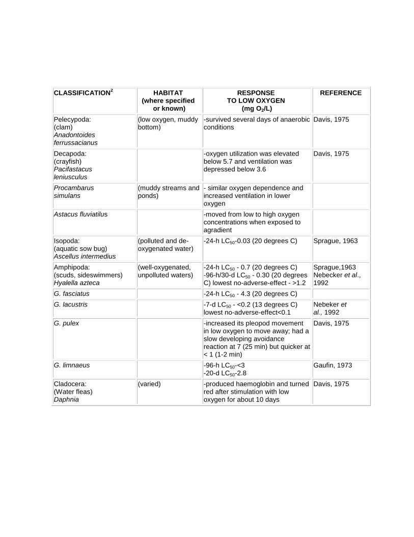
CLASSIFICATION2 HABITAT
(where specified or known)
RESPONSE TO LOW OXYGEN
(mg O2/L)
REFERENCE
Pelecypoda: (clam) Anadontoides ferrussacianus
(low oxygen, muddy bottom)
-survived several days of anaerobic conditions
Davis, 1975
Decapoda: (crayfish) Pacifastacus leniusculus
-oxygen utilization was elevated below 5.7 and ventilation was depressed below 3.6
Davis, 1975
Procambarus simulans
(muddy streams and ponds)
- similar oxygen dependence and increased ventilation in lower oxygen
Astacus fluviatilus -moved from low to high oxygen concentrations when exposed to agradient
Isopoda: (aquatic sow bug) Ascellus intermedius
(polluted and de-oxygenated water)
-24-h LC50-0.03 (20 degrees C) Sprague, 1963
Amphipoda: (scuds, sideswimmers) Hyalella azteca
(well-oxygenated, unpolluted waters)
-24-h LC50 - 0.7 (20 degrees C) -96-h/30-d LC50 - 0.30 (20 degrees C) lowest no-adverse-effect - >1.2
Sprague,1963 Nebecker et al., 1992
G. fasciatus -24-h LC50 - 4.3 (20 degrees C)
G. lacustris -7-d LC50 - <0.2 (13 degrees C) lowest no-adverse-effect<0.1
Nebeker et al., 1992
G. pulex -increased its pleopod movement in low oxygen to move away; had a slow developing avoidance reaction at 7 (25 min) but quicker at < 1 (1-2 min)
Davis, 1975
G. limnaeus -96-h LC50-<3 -20-d LC50-2.8
Gaufin, 1973
Cladocera: (Water fleas) Daphnia
(varied) -produced haemoglobin and turned red after stimulation with low oxygen for about 10 days
Davis, 1975

CLASSIFICATION2 HABITAT
(where specified or known)
RESPONSE TO LOW OXYGEN
(mg O2/L)
REFERENCE
D. magna -preferred fully saturated water over water 15 percent saturated although more than an hour was required for the response to develop -1.8 reduced fecundity in 26-d -2.7 reduced final weight by 17% -3.7 had no effect -48-h LC50 - 0.6, 0.7 (12 degrees C) -lowest no-adverse-effect 0.9
Homer and Waller, 1983
Nebeker et al., 1992
D. pulex -48-h LC50 - 0.5 (17 degrees C) -96-h LC50 - 0.4 and 0.7 -lowest no-adverse-effect 2.1 (based on reproduction)
Nebeker et al., 1992
Coleoptera: Ephemeroptera (Mayflies)
-Critical oxygen tension (Pc) below which respiratory dependence occurred:
Davis, 1975
Baetis (swift streams) 17.00
Leptophlebia (lakes) 3.60
Cloean (ponds) 2.86 -96-h LC50 at 18.5 degrees C:
Nebeker,1972
Hexagenia limbata 1.4
Baetisca laurentina 3.5
L. nebulosa 2.2
Ephemerella subvaria 3.9
Ephemera simulans -30-d LC50 at 18.5 degrees C: 4.5
B. laurentina 5.0
L. nebulosa -% emergence at mg O2/L: 70/20/0 9.0/6/2.4
B. laurentina 70/0 7.0/4.0
E. simulans 40/0 9.0/4.1
Plecoptera: (Stoneflies) Pteronarcys
(well-oxygenated, moving water)
-96-h LC50: 2.2 (18.5 degrees C)
Nebeker, 1972
Acroneuria lycoria -96-h LC50: 3.6 (14 degrees C) -30-day LC50:

CLASSIFICATION2 HABITAT
(where specified or known)
RESPONSE TO LOW OXYGEN
(mg O2/L)
REFERENCE
P. dorsata 4.4-4.8
Trichoptera: (caddis flies) Hydropsyche betteni
(well-oxygenated water)
-96 h LC50: 2.9 (21.0 degrees C) 2.6 (18.5 degrees C) 2.3 (17.0 degrees C) 1.0 (10.0 degrees C)
Nebeker, 1972
Coleoptera: (beetle) Donacia
(emergent vegetation)
-became less active in low oxygen; survived 168 h in closed bottles that initially contained 0.37
Davis, 1975
Diptera: (midges) Chironomids
(bottom organisms) -regulated oxygen uptake and lowered Pc following acclimation to low oxygen -suspended feeding when oxygen levels dropped to 5-7.5 percent of saturation
Davis, 1975
Chironomus authracinus
-at 1, growth stopped (limited respiration produced only enough energy for maintenance of vital functions)
Tanytarsus dissimilis
(sluggish water) -96-h LC50 at 18.5 degrees C: <0.6 -30-d LC50 at 18.5 degrees C: <0.6 -% emergence at mg O2/L: 80+/0 <0.6/0
Nebeker, 1972
1 Some species may not be native to British Columbia
2 Species are grouped under commonly used group classifications (usually Orders but in some cases
Phyllum names are used)
Nebeker (1972) investigated low oxygen tolerances of insects known to be important fish food (larvae of stoneflies, mayflies, caddis flies and midges). In addition to the 96-h LC50 analyses, he also looked at the more meaningful 30-day survival and emergence success (Table 4). One species of mayfly (Baetisca laurentina) and one stonefly (Pteronareys darsata), tested in both time sequences, were less tolerant of the 30-day exposure to low oxygen than of the 96-hour routine, while a chironomid (Tanytarsus dissimilis) accustomed to low oxygen showed no difference in response. Adult emergence also was inhibited at much higher percentage saturations than the 96-h LC50values. For example, the mayfly Leptophlebia nebulosa had 70 percent emergence at 9.0 mg O2/L (saturation at 18.5 degrees C would have been 9.3 mg/L), 20 percent emergence at 6.0 mg/L and no emergence at less than 2.4 mg/L. The midge Tanytarsus dissimilis was least sensitive to low oxygen and could reproduce (with greater

than 80% emergence) at concentrations as low as 0.6 mg/L. Nebeker advocated full life cycle studies for the examination of oxygen stress on aquatic insects.
Subsequent to the release of the 1986 US EPA criteria document on dissolved oxygen, Nebeker et al. (1992) collected additional invertebrate data on long-term exposure to hypoxia at high summer temperatures and at concentrations simulating natural levels in the field (used diurnal fluctuations). The LC50 acute response thresholds reported in Table 4 for the four species chosen (two cladocerans and two amphipods) were all below 1 mg/L. Chronic tests over 5 to 30 days considered significant differences (p<0.05) in survival, growth or reproduction, from control groups. Chronic response thresholds in terms of lowest no-adverse-effect varied from a low of 0.9 mg O2/L to a high of 2.1 mg O2/L (based on reproduction) for the four species. The investigators noted that the animals stayed at or near the surface to expose parts of their body to the air when subjected to lethal dissolved oxygen levels. They concluded that the representatives from the two large groups of crustaceans were relatively tolerant of hypoxia and the present criterion (US EPA, 1986) for freshwater aquatic life (Table 11) would provide reasonable protection for these invertebrates.
4.2.2 Marine
Davis (1975) also reviewed the effects of low oxygen in marine and brackish environments. Table 5 largely summarizes his discussion of oxygen requirements of intertidal, benthic, and pelagic invertebrates.
During low tide, surface organisms are either exposed entirely or left in pools, which may experience considerable oxygen demand from algae and become anoxic. As expected, groups which occupy this zone tend to be highly resistant to oxygen deficiency (Table 5-i). Organisms living on or within mud flats are particularly tolerant, while those on exposed, firm substrates are usually less tolerant of oxygen stress. Parasado Rao and Ganapati (1968) identified the critical oxygen tension (Pc) in two barnacles, one adapted to oxygen-rich areas (Pc=5.0 mg/L) and the other to polluted habitats (Pc=3.5 mg/L). Oxygen dependence occurred below these levels and no gaseous exchange was found below 0.7 mg/L (anaerobiosis likely was possible for short periods). Sassaman and Mangum (1972) found similar results for two species of anemones with different oxygen requirements (the burrowing form consumed less and had greater tolerance of oxygen stress). The researchers noted that both test animals could survive anoxia much longer than the normal tidal cycle. This also appears to be true of many intertidal taxa listed in Table 5, which have demonstrated resistance to anoxia, or at least very low oxygen levels (less than 1 mg/L) for extended periods.
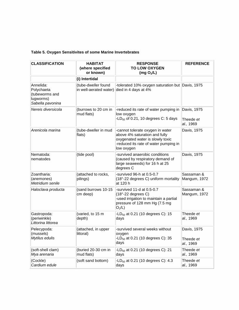
Table 5. Oxygen Sensitivites of some Marine Invertebrates
CLASSIFICATION HABITAT (where specified
or known)
RESPONSE TO LOW OXYGEN
(mg O2/L)
REFERENCE
(i) Intertidal
Annelida: Polychaeta (tubeworms and lugworms) Sabella pavonina
(tube-dweller found in well-aerated water)
-tolerated 10% oxygen saturation but died in 4 days at 4%
Davis, 1975
Nereis diversicola (burrows to 20 cm in mud flats)
-reduced its rate of water pumping in low oxygen -LD50 of 0.21, 10 degrees C: 5 days
Davis, 1975
Theede et al., 1969
Arenicola marina (tube-dweller in mud flats)
-cannot tolerate oxygen in water above 4% saturation and fully oxygenated water is slowly toxic -reduced its rate of water pumping in low oxygen
Davis, 1975
Nematoda: nematodes
(tide pool) -survived anaerobic conditions (caused by respiratory demand of large seaweeds) for 16 h at 25 degrees C
Davis, 1975
Zoantharia: (anemones) Metridium senile
(attached to rocks, pilings)
-survived 96-h at 0.5-0.7 (18°-22 degrees C) uniform mortality at 120 h
Sassaman & Mangum, 1972
Haloclava producta (sand burrows 10-15 cm deep)
-survived 11-d at 0.5-0.7 (18°-22 degrees C) -used irrigation to maintain a partial pressure of 128 mm Hg (7.5 mg O2/L)
Sassaman & Mangum, 1972
Gastropoda: (periwinkle) Littorina littorea
(varied, to 15 m depth)
-LD50 at 0.21 (10 degrees C): 15 days
Theede et al., 1969
Pelecypoda: (mussels) Mytilus edulis
(attached, in upper littoral)
-survived several weeks without oxygen -LD50 at 0.21 (10 degrees C): 35 days
Davis, 1975
Theede et al., 1969
(soft-shell clam) Mya arenaria
(buried 20-30 cm in mud flats)
-LD50 at 0.21 (10 degrees C): 21 days
Theede et al., 1969
(Cockle) Cardium edule
(soft sand bottom) -LD50 at 0.21 (10 degrees C): 4.3 days
Theede et al., 1969

CLASSIFICATION HABITAT (where specified
or known)
RESPONSE TO LOW OXYGEN
(mg O2/L)
REFERENCE
(i) Intertidal
(Oyster) Ostrea virginica
(attached, in upper littoral)
-survived less than 0.5 for at least one week
Davis, 1975
Thoracia: (barnacles) Balanus amphitrite
(polluted, oxygen deficient areas)
-respiratory regulation ceased at 3.5 and metabolic rate decreased along with oxygen levels below this
Parasada Rao and Ganapati, 1968
B. tintinnabulum (oxygen-rich open areas)
-respiratory regulation ceased at 5.0 and metabolic rate decreased along with oxygen levels below this
Parasada Rao and Ganapati, 1968
Amphipoda: (gammarids) Gammarus oceanicus
(tidepool) -avoids anoxic conditions and becomes more active in low oxygen -LD50 at 0.21 (10 degrees C): 15 h
Davis, 1975
Theede et al., 1969
Allorchestes angustus (under rocks, logs, algae)
-tolerated 0.3-0.89 in surface water near a pulp mill
Davis, 1975
Anisogammarus pugettensis A. confervicolus
-survived 24 h at 0.24-1.8 but died after 36 h
Davis, 1975
Decapoda: (crabs) Uca pugnax U. pugilator
(marsh) -respiratory-independent to a partial pressure of 40-50 mm Hg (2.6 mg O2/L) and withstood anaerobic condi-tions for at least one week
Davis, 1975
Echinoidea: (urchins) Strongylocentrotus drobachienis S. franciscanus S. purpuratus
(hard bottoms) -can be various degrees and modes of respiration related to oxygen availability and metabolic demand -respiratory-dependent below 60-70 mm Hg (4.7 mg O2/L) oxygen partial pressure
Davis, 1975
Asteroidea: (sea stars) Asterias rubens
(hard bottoms) -LD50 at 0.21 (10 degrees C): 4.3 days
Theede et al., 1969
ii) Benthic
Annelida: Polychaeta (tubeworms, lugworms) Hydroides norvegica
(burrows) -showed reduced larval settlement in low oxygen
Davis, 1975
Chaetopterus variopedatus
(burrows) -increased its rate of pumping in burrows
Cnidaria: (anenome) Actinia
(hard surfaces) -migrated to the surface when oxygen fell below 2.0
Davis, 1975

CLASSIFICATION HABITAT (where specified
or known)
RESPONSE TO LOW OXYGEN
(mg O2/L)
REFERENCE
(i) Intertidal
Cephalopoda: (octopus) Octopus dofleini
(sheltered areas) -exhibited lowered arterial blood oxygen levels and elevated cardiac output when oxygen partial pressure dropped below 120 mm Hg (8.42 mg O2/L)
Davis, 1975
Isopoda: (isopods) Limnoria lignorum L. quadripunctata L. tripunctata
(in wood) -burrowing activity was directly related to available oxygen; 28 day TLm for three temperatures ranged from 0.6-1.18
Davis, 1975
Idotea baltica (sand bottom) -LD50 at 0.21 (10 degrees C Theede et al., 1969
Amphipoda: (amphipods) Corophium arenarium
(aerobic sediments) -exhibited a preference for oxygenated water
Davis, 1975
C. volutator (anaerobic sediments)
-no preference for oxygen levels in water
Stomatopoda: (mantis Shrimp) Squilla mantis
-showed elevated respiratory movements in low oxygen
Davis, 1975
Decapoda: (crab) Cancer productus
-demonstrated oxygen-dependent respiration particularly at high temperatures
Davis, 1975
Carcinus maenas -elevated respiratory movements in low oxygen -LD50 at 0.21 (10 degrees C): 2 days
Theede et al., 1969
(shrimp) Crangon vulgaris
-asphyxiated below 20% air saturation, migrated vertically at 22-35% saturation
Huddard and Arthur, 1971
Crangon crangon (prawn) Pandalus borealis
(sound bottom) -LD50 at 0.21 (10 degrees C): 2 h
-elevated respiratory movements in low oxygen
Theede et al., 1969 Davis, 1975
Ophiuroidea: (brittle star) Ophiura albida
(on sand/silt bottom) -LD50 at 0.21 (10 degrees C): 1.3 days
Theede et al., 1969
(iii) Pelagic
Mysidacea: (opossum shrimp) Gnathophausia ingens
(intermediate depth, stable oxygen-minimum layers)
-regulated oxygen consumption and respired aerobically down to 0.3
Childress, 1971

CLASSIFICATION HABITAT (where specified
or known)
RESPONSE TO LOW OXYGEN
(mg O2/L)
REFERENCE
(i) Intertidal
Copepoda: (copepods) Calanus plumchrus
-were very abundant in an oxygen minimum layer (0.57 mg/L) in Saanich Inlet -another researcher reported Calanus was killed at between 1.4-2.9
Davis, 1975
Euphausiacea: (krill) Euphausia pacifica
-would not enter an oxygen minimum layer (0.57 mg/L) in Saanich Inlet
Davis, 19765
Cephalopoda: (squid) Loligo
-avoided oxygen-deficient water Davis, 1975
Benthic marine invertebrates are associated with a variety of habitats (Table 5-ii), many of which may be oxygen-deficient due to the consumptive demands present at the substrate. The oxygen requirements of these organisms, like their freshwater counterparts, usually are tailored to their particular habitats. Oxygen-dependent respiration and behavioural changes are common in reduced oxygen. For example, Huddard and Arthur (1971) (cited in Davis, 1975) found that shrimps (Grangon cullgaris) swim upwards at dissolved oxygen levels between 22 and 35 % saturation, presumably to be displaced by currents to more oxygenated water where they passively sink to the bottom. Elevated respiratory movements in response to low oxygen are typical of burrowing polychaete worms and many crustaceans, although the reverse also is found (Davis, 1975) (see Table 5-ii). Hoos (1973) (cited in Davis, 1975) determined that benthic species diversity decreased with depth and varied seasonally according to the oxygen level. Levings (1972) (unpublished data in Davis, 1975) found 20 polychaete taxa at one station greater than 150 m deep in Howe Sound where oxygen content typically was 2.9 to 4.3 mg/L. Alternatively, Levings and McDaniel (1964) (cited in Davis, 1975) sampled a diverse community of epifaunal invertebrates attached to a cable retrieved from 300 m to 500 m depths in the Strait of Georgia. Thompson (1981) also reported a thriving benthic community of polychaete worms, brittle stars, crabs, urchins and clams from the western basin of Johnstone Strait. This productivity was attributed to the strong bottom currents that moved freshly-oxygenated water over the channel floor and maintained uniform oxygen concentrations year-round. The absence of this circulation behind silled basins and fiords keeps faunal diversity depressed in those areas due to the devastating effects of hypoxia.
Pelagic invertebrates also may encounter a variety of oxygen conditions, and their requirements and behavioural responses related to oxygen more closely resemble higher life forms such as pelagic fish (Davis, 1975). As indicated in Table 5-iii, avoidance reactions to oxygen deficiency are common in groups which swim freely. Many organisms also become adapted to low-oxygen strata. Davis (1975) cited a study by Hoos (1970), in which 27 species inhabited an oxygen-minimum layer (0.57 mg/L) in Saanich Inlet. Childress (1971) reported that a mysoid (Gnathophausia ingens) could respire aerobically in oxygen levels as low as 0.3 mg/L rather than revert to anaerobiosis. Such an adaptation likely was possible because of the long-term uniformity of water quality conditions where it is found.

4.3 Effects on Fish
4.3.1 Introduction
The bulk of available literature on the dissolved oxygen requirements for aquatic life deals with freshwater and anadramous salmonids. This is understandable, given the economic benefits derived from both natural and artificially propagated stocks. With respect to the latter, much research has been directed at early life stages for the purpose of optimizing ambient conditions for hatchery production. Comparatively few data exist for strictly marine fishes found in proximity to the British Columbia coastline. Davis (1975) presented a small amount of marine-related data in his oxygen criteria document and, of these, most referred to Atlantic or European species.
The Appendix contains a list of the principal fishes considered in the derivation of criteria for this document. It is obvious that this listing is primarily based upon coldwater salmonids (the Esocidae being an exception). Available evidence suggests that some non-salmonids may be at least as sensitive to low dissolved oxygen as salmonids. The US EPA considers the herrings, smelts, pikes and sculpins to be among those groups, while several warmwater families (many introduced) found in this province such as basses, sunfishes, catfishes and perches generally are more tolerant of lower oxygen levels. For diverse environments such as covered by national criteria (e.g., CCME, 1987; US EPA, 1986; Davis, 1975) it is common to have dichotomies with respect to coldwater/warmwater species and salmonid/non-salmonid species. In British Columbia, coldwater fishes with similar sensitivities inhabit essentially all watersheds, although warmwater species may co-exist. It was considered redundant to have separate criteria for warmwater fishes, which admittedly are a more biologically diverse and less well-understood grouping. However, a criterion predicated on the requirements of coldwater salmonids (and like-salmonids) should protect non-salmonids.
Recent criteria documents have recognized two distinct salmonid habitats (with characteristic dissolved oxygen regimes) associated with two distinct development stages. The oxygen requirements and oxygen supply to early life stages (buried eggs through to emergence or a post-hatch period) are different from those for free-swimming, later life stages which reside in the water column. This document deals first with juvenile/adult life stages (including free-swimming fry that may have residual yolk sac material), followed by embryo/alevin life stages. The early development stages for salmonids are described by a variety of nomenclatures by different authors, which can lead to confusion. For the purpose of this discussion, fertilized eggs are considered embryos up until the time of hatch and alevins are semi-mobile with yolk sacs, but still reside within the gravel interstices (some may refer to these stages as simply all embryonic or larval).
4.3.2 Juvenile / Adult Life Stages
Data in the literature on the effects of low dissolved oxygen on fish are highly variable and sometimes contradictory due largely to the absence of standardized analytical methods (e.g., 96-h LC50 test is seldom used). Different experimental apparatus, water temperatures, flow rates, acclimation periods, exposure times and feeding characteristics have been used. Further variability is introduced by the different oxygen sensitivities between species and within different life stages of the same species, and for different behaviour/metabolic processes (e.g., swimming, feeding, growth, bioenergetics).

The following sections on acute and chronic toxicity of hypoxia to fish will focus on studies considered to be the most definitive by other reviewers and noted experts in the field.
4.3.2.1 Acute Effects
Oxygen lethality thresholds reported in the literature are particularly dependent on experimental design. Researchers have utilized a variety of procedures to develop hypoxic conditions (e.g., placing fish in sealed vessels where respirated oxygen is not replaced, addition of nitrogen to bind dissolved oxygen, boiling, drawing naturally deoxygenated water from wells or in situ tests in hypolimnetic layers). These techniques all have varying degrees of susceptibility to interferences from other common variables such as ammonia and dissolved gasses. For example, the presence of high concentrations of carbon dioxide (inherent in closed vessel tests) commensurate with high pH and alkalinity will increase the tolerance of coho salmon to low oxygen (Warren et al., 1973).
The dosing technique also is important. Fish may have been subjected to a sudden drop in dissolved oxygen or step-down concentrations. Where reductions have been gradual, the ability of some fish to acclimate through a physiological adjustment (which improves blood oxygen carrying capacity) has been observed. Studies by Shepard (1955) on brook trout suggested a simple straight-line relationship between higher incipient (first occurring) lethal levels and acclimation levels. However, regardless of acclimation history, age group or state of activity, the entire range of lethality occurred within a relatively narrow interval of 1.4 mg O2/L oxygen. The lowest concentration to which trout were acclimated was 1.05 mg O2/L and the incipient lethal level was approximately 1.85 mg O2/L.
Wirosoebroto-Hartadi's (1986) work on rainbow trout yielded similar results and found consistently lower lethality thresholds for acclimated rainbow trout. The mean difference in LC50s for fish acclimated to 6 mg O2/L and 4.2 mg O2/L was about 0.3 mg O2/L. It was also noted that step-down dosing of non-acclimated fish resulted in an acclimation-type response in itself. Douddoroff and Shumway (1970) gave a detailed account of these and other variables (exposure time, water temperature, age and size of test subjects, accessibility to surface/air interface, etc.) encountered in lethality studies. These authors acknowledged that published test results were not often comparable and the practical significance of most were questionable. Nevertheless, the ranges of low oxygen tolerances ascribed to various fish species are of interest.
Table 6 contains the results of the lethality studies cited above and others considered to be representative of local species. As other reviews (Doudoroff and Shumway, 1970; EIFAC, 1973; US EPA, 1986) have established, observed lethal oxygen levels generally increased at higher water temperatures and longer exposures, and mortality or loss of equilibrium occurred between 1 and 3 mg/L; reported laboratory results outside of this range should be considered suspect.
4.3.2.2 Chronic Effects
The problems cited previously with interpreting the literature on dissolved oxygen effects are probably most pronounced for chronic toxicity. The manner and intensity of fish responses to hypoxia can vary widely among studies on the same bodily functions. This document has adopted the premise of other reviewers (US EPA, 1986; Davis, 1975) that consistent effects (behavioural, physiological or other) first observed at higher concentrations must take precedence for criteria purposes, over test results that have
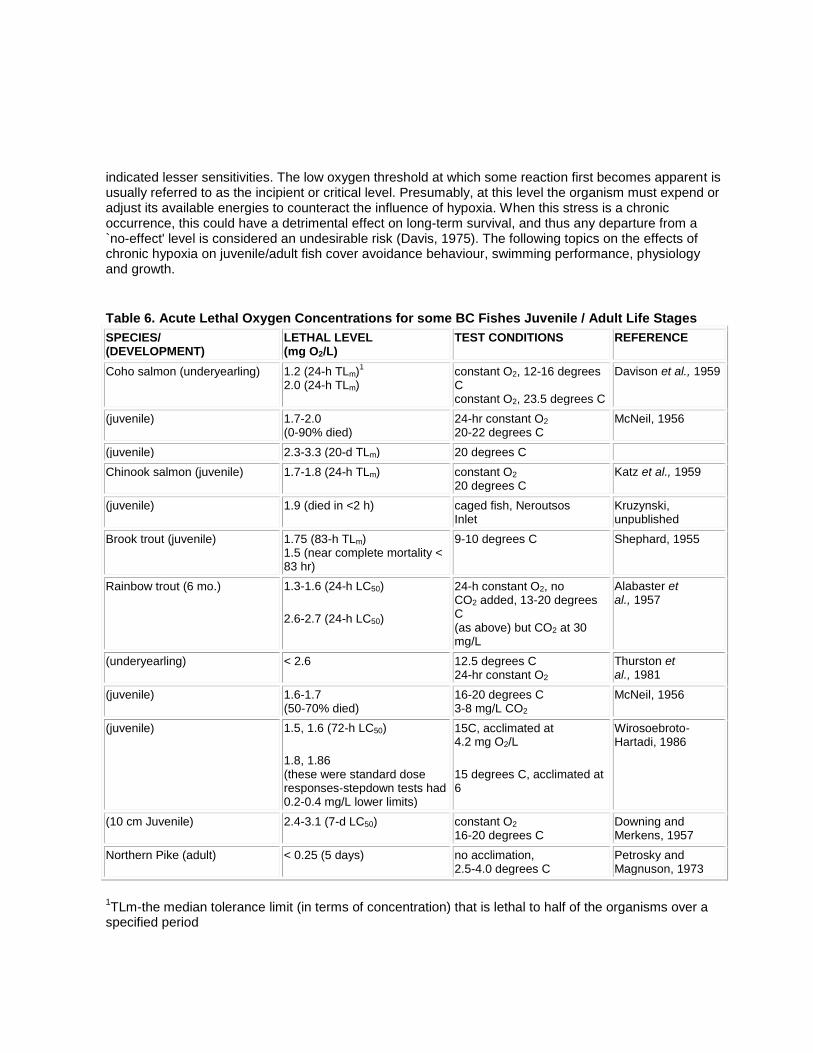
indicated lesser sensitivities. The low oxygen threshold at which some reaction first becomes apparent is usually referred to as the incipient or critical level. Presumably, at this level the organism must expend or adjust its available energies to counteract the influence of hypoxia. When this stress is a chronic occurrence, this could have a detrimental effect on long-term survival, and thus any departure from a `no-effect' level is considered an undesirable risk (Davis, 1975). The following topics on the effects of chronic hypoxia on juvenile/adult fish cover avoidance behaviour, swimming performance, physiology and growth.
Table 6. Acute Lethal Oxygen Concentrations for some BC Fishes Juvenile / Adult Life Stages
SPECIES/ (DEVELOPMENT)
LETHAL LEVEL (mg O2/L)
TEST CONDITIONS REFERENCE
Coho salmon (underyearling) 1.2 (24-h TLm)1
2.0 (24-h TLm)
constant O2, 12-16 degrees C constant O2, 23.5 degrees C
Davison et al., 1959
(juvenile) 1.7-2.0 (0-90% died)
24-hr constant O2 20-22 degrees C
McNeil, 1956
(juvenile) 2.3-3.3 (20-d TLm) 20 degrees C
Chinook salmon (juvenile) 1.7-1.8 (24-h TLm) constant O2 20 degrees C
Katz et al., 1959
(juvenile) 1.9 (died in <2 h) caged fish, Neroutsos Inlet
Kruzynski, unpublished
Brook trout (juvenile) 1.75 (83-h TLm) 1.5 (near complete mortality < 83 hr)
9-10 degrees C Shephard, 1955
Rainbow trout (6 mo.) 1.3-1.6 (24-h LC50)
2.6-2.7 (24-h LC50)
24-h constant O2, no CO2 added, 13-20 degrees C (as above) but CO2 at 30 mg/L
Alabaster et al., 1957
(underyearling) < 2.6 12.5 degrees C 24-hr constant O2
Thurston et al., 1981
(juvenile) 1.6-1.7 (50-70% died)
16-20 degrees C 3-8 mg/L CO2
McNeil, 1956
(juvenile) 1.5, 1.6 (72-h LC50)
1.8, 1.86 (these were standard dose responses-stepdown tests had 0.2-0.4 mg/L lower limits)
15C, acclimated at 4.2 mg O2/L
15 degrees C, acclimated at 6
Wirosoebroto-Hartadi, 1986
(10 cm Juvenile) 2.4-3.1 (7-d LC50) constant O2 16-20 degrees C
Downing and Merkens, 1957
Northern Pike (adult) < 0.25 (5 days) no acclimation, 2.5-4.0 degrees C
Petrosky and Magnuson, 1973
1TLm-the median tolerance limit (in terms of concentration) that is lethal to half of the organisms over a
specified period

Avoidance Behaviour - The severity of hypoxic conditions may be much less if affected organisms can sense and avoid localized areas of depressed oxygen; however, this in itself can have serious consequences. Birtwell (1989) reported that much of the chum salmon run was prevented from reaching spawning streams at the head of Neroutsos Inlet. Many salmon that were delayed were too far advanced in maturity to spawn successfully had they been able to complete their migration. McGreer and Vigers (1983) found avoidance reaction in juvenile chum salmon up to 10 km from the Port Alice pulp mill (northern Vancouver Island) partially as a result of severely depleted dissolved oxygen conditions in Neroutsos Intlet. However, these workers also determined that pH had a greater influence on fish avoidance behaviour, which suggested the effluent itself was also involved in stimulating avoidance (mortalities were found up to 2 km from the discharge). Alabaster (1989) suggested that migrating chinook salmon in the San Joaquin Delta region of California were severely impeded at dissolved oxygen levels below 3.5 mg/L. Records of chinook salmon ascending the somewhat polluted Willamette River in Oregon were compared to known oxygen concentrations (Alabaster, 1988). Summer run numbers were expressed by way of percentile distributions to define the failure or success of a portion of the run passing a known point of lowest dissolved oxygen content and then travelling upstream to the Willamette Falls. The division point between most of the fish running, relative to when most were not, corresponded to an oxygen level of about 3.5 mg/L over four consecutive years. Migration did not appear to be inhibited in one year when the average daily minimum was about 5.7 mg O2/L. A well-known study by Whitmore et al. (1960) on chinook and coho salmon in troughs identified a seasonal variability, whereby juvenile chinook salmon avoided oxygen concentrations from 1.5 to 4.5 mg/L in summer (water temperature 18C), but did not avoid 4.5 mg/L in autum (water temperature 12C). Alternatively, coho salmon avoided all oxygen concentrations below 6 mg/L in summer, but were less consistent in their responses. Both species exhibited a marked preference for 9 mg O2/L or higher. Birtwell and Kruzynski (1989) reported that underyearling chinook salmon avoided dissolved oxygen below 7 to 8 mg/L. Shephard (1955) reported violent activity and attempts to surface by brook trout subjected to low oxygen (0.5-1.9 mg/L). Davis (1975) explained that a non-acclimated fish might well react in this way as a survival response, but acclimation could lower the magnitude of this response to conserve energy. Spoor's (1989) more recent work on brook trout offered fingerlings (fed and acclimated) the choice of a wide range of oxygen concentrations in 16 gradients between 1 and 8.9 mg/L. They avoided concentrations below 4 mg/L and preferred 5 mg/L or higher with statistical certainty. However, given the choice of any of two concentrations above 5 mg/L, the fish did not show a significant preference for the higher of the two.
Wirosoebroto-Hartadi (1986) investigated the importance of surface access to rainbow trout survival when fish were subjected to severe oxygen reductions. Surfacing/gulping behaviour, was observed which was interpreted as alternate respiration activity. Fish succumbed earlier and in greater numbers when screened from the air-water interface, although it was cautioned that this also could have been a consequence of the increased stress presented by the blockage. Gee et al. (1978) observed northern pike, in progressive hypoxia, to rise to the surface and utilize the more well-oxygenated surface film, while two salmonid species under the same circumstances did not exhibit this behaviour. Similarly, Petrosky and Magnuson (1973) exposed pike in sealed aquaria to lower oxygen successively (4.0, 2.0, 1.0, 0.5 and 0.25 mg/L at 2.5 to 4.0 degrees C) each day for five days under simulated winter-kill conditions. The fish moved upward (usually the most well-oxygenated water in natural situations) at 0.5 mg/L and 'nosing activity' was observed at 0.25 mg/L. Nosing allows fish to utilize thin layers of oxygenated water at the surface (whether ice covered or not). This behaviour also was observed by Magnuson and Karlen (1970) beneath the ice in a lake where winter-kill has occured. Pike took up residence in domes that they formed in the under-surface of the ice.

Avoidance behaviour and vertical migration/nosing activity have obvious survival benefits, but the physiological control mechanism is not understood. Several researchers have shown that circulatory and ventilatory reactions to hypoxia are rapid and may themselves be the trigger for behavioural response, or a direct receptor system near the gills may be responsible (Davis, 1975). It is known that detection of an oxygen gradient is not necessary to elicit a surfacing tendency, and interference from high carbon dioxide or hydrogen sulphide levels can be ruled out. Typically, an avoidance response is coupled with increased locomotory activity, which is discussed in the next section. Regardless of the process involved, the capacity for avoidance should not have a bearing on the development of criteria (with respect to making them less stringent). As the US EPA (1986) cautioned, if space or food resources are limited, avoidance could affect fish almost as seriously as direct mortality.
Swimming Performance - Swimming activity may increase or decrease in response to lowered dissolved oxygen, and if the first occurs it is often followed by the second (EIFAC, 1973). Doudoroff and Shumway (1970) considered that increased random movement elicited by hypoxia, followed by more tranquil behaviour in well-oxygenated water, constituted avoidance of low oxygen. As discussed in the previous section, avoidance behaviour which may be directed to some degree to areas of improved oxygen, can be very active at low oxygen concentrations and warm water temperatures (Shephard, 1955; Petrosky and Magnuson, 1973; Whitmore et al., 1960). Even when the oxygen level approached lethality, Magnuson and Karlen (1970) observed that Northern pike under ice cover sounded more frequently into anoxic water during their final days. This behaviour and those observed for fish subjected to extreme oxygen gradients during labortory studies might be considered desperate and in some cases exaggerated from the norm. The predominant response to progressive hypoxia is a decrease in locomotory activity.
Researchers have examined the ability of fish to maintain moderate swimming speeds for extended periods under low oxygen conditions. For example, Katz et al. (1959) showed that juvenile chinook and coho salmon were able to swim continuously against a current of 24 cm/s for one day and two days, respectively, at oxygen concentrations near 3 mg/L. More detailed relationships between the swimming performance of salmonids and oxygen concentration have been developed by determining the percent reduction of maximum sustainable speeds over a range of oxygen levels and temperatures. Jones (1971) subjected juvenile rainbow trout to increasing water velocities to determine fatigue levels under two temperature regimes (14.1 degrees C and 22.4 degrees C) at 50 % saturation. The low temperature group registered a 43 % decline in sustainable swimming speed at an oxygen concentration of 5.2 mg/L (half-saturation) and the high temperature group suffered a 30 % performance drop at 3.9 mg/L (Figure 4).
The greater impairment at higher oxygen concentrations is somewhat surprising, although a reduction to half-saturation for that group represented a greater absolute drop in oxygen content. Also, it is important to understand that the Jones study (1971) was tailored to measure a temperature effect on swimming rather than different degrees of hypoxia. He noted that the haematocrit level, a measure of blood oxygen carrying capacity, was significantly higher in the high temperature group. High temperature hypoxia, in general, appeared to complicate the relationship between the metabolic cost of both cardiac and branchial pumps. The level of impairment experienced by the higher temperature group was comparable to results obtained in similar studies (See Figure 4) on coho salmon by Davis et al. (1963) and Dahlberg et al. (1968). Dahlberg et al. (1968) purposely chose the same test period (10 minutes) for final swimming velocities and similar ambient water temperatures and carbon dioxide levels (low) as Davis et al. (1963) to facilitate comparisons. Accordingly, Dahlberg et al. (1968) found a similar response curve which showed a progressive deterioration in maximum sustainable swimming performance as dissolved

oxygen levels dropped below 8 mg/L. Both study groups tested oxygen levels higher than air saturation (>9.1 mg/L at 20 degrees C) and found little or no effect on swimming performance. When temperature alone was varied, Davis et al. (1963) found performance, at any given oxygen concentration, improved modestly but steadily from 10 to 20 degrees C. Bushnell et al. (1984) determined the critical (sustainable) swimming speed for rainbow trout to be 54.8 cm/s, when acclimated to an oxygen level near saturation at 15 degrees C. Reduction of ambient oxygen to 3.9 and 2.6 mg/L, resulted in corresponding impairment of critical swimming speeds by 6 % and 25 % respectively (Figure 4). A second set of hypoxia-acclimated fish exhibited no improvement in response to lowered oxygen. Bushnell et al. (1984) noted that the critical speed obtained under well-oxygenated conditions likely was underestimated somewhat due to water speed limitations of their apparatus (impairment would be underestimated proportionally). This might explain the considerable difference (higher) in impairment level recorded by Jones (1971) at an identical oxygen level and similar temperature. In conclusion, the coho swimming performance data of Davis et al. (1963) and Dahlberg et al. (1984) were presented with fewer compromises and qualifications and appear to be more reliable than the rainbow trout studies included in Figure 4.
Figure 4. Effects of Dissolved Oxygen on Maximum Sustainable Swimming Performance of some Salmonids
Mechanisms which respond to chronic hypoxia and evoke physical reaction such as decreased swimming performance are not well understood. Dahlberg et al. (1968) suggested that oxygen uptake at low oxygen concentrations is predominantly determined by the maximum possible rate of gill irrigation as opposed to the oxygen transport capacity of the blood which largely is unutilized in these circumstances. At some point of reduced ambient oxygen concentration, maximum irrigation cannot keep the blood fully oxygenated and the level of sustainable activity will decline.
The ecological significance of slight impairment of swimming performance is difficult to assess. Davis et al. (1963) commented that fish are not likely to possess performance capabilities that do not contribute to their success or well-being. Intuitively, any decrease in sustainable swimming ability would adversely affect related demands such as feeding, reproduction, escape from predation and upstream migration.
Physiology and Bioenergetics - Molecular oxygen is vital for much of the oxidative, energy-producing metabolism of fish, and as such can operate as a limiting factor. Much work has been directed at determining the minimum level of ambient oxygen that begins to limit the rate of oxygen uptake. Although respiratory and cardio-vascular effects in organisms represent the root responses to hypoxia, there have been considerable difficulties in isolating cause and effect relationships and deciding what constitutes impairment of vital functions. For example, oxygen demands of normal metabolic processes such as feeding and digestion might result in similar oxygen demands in blood or tissues as when a fish experiences hypoxia. The maximum steady swimming speed of a fish was assumed to be closely related to the `scope for activity'- a term described by Fry (1957) meaning the difference between the standard and active oxygen uptake rate. It is an indirect measure of the relative capacity of a fish to sustain work as in the maintenance of steady muscular activity. One of the most exhaustive discussions of physiological responses to low oxygen is contained in Doudoroff and Shumway (1970). The authors concluded that because there was sufficient discrepancy between conclusions drawn from reported oxygen uptake rates and swimming speed data or on amounts of energy expended by active fish, that it was best to rely on direct measurements of swimming performance in evaluating the influence of water quality.
Notwithstanding the persistent problems of consistency in bioenergetic investigations, they are useful in revealing some of the underlying mechanisms directing the more dynamic responses to hypoxia. The early conceptual relationships of Fry (1957) continue to be referenced (e.g., Davis, 1975), particularly that of oxygen concentration versus oxygen uptake illustrated in Figure 5. He explained that above a critical `incipient limiting level' is a `zone of respiratory independence' where the maximum rate of oxygen uptake is unaffected by oxygen concentration. Below this no-effect threshold is the `zone of respiratory dependence' where a decrease in environmental oxygen is accompanied by a decrease in uptake, to a point (incipient lethal level) at which minimum oxygen requirem4nts cannot be met. This lethality level divides a `zone of resistance', where organisms may survive for a limited time, and a `zone of tolerance' where they will survive indefinitely. The curve obviously is species-dependent and is affected by environmental variables. In animals less tolerant of low oxygen, the curve is shifted to the right (and vice-versa)(Davis, 1975; Shephard, 1955). Virtually any factor that influences the metabolic rate of fish will affect the curve (e.g., temperature, level of activity, nutritional state, respiratory, circulatory acclimation, etc.) (Doudoroff and Shumway, 1970). While it is generally accepted that the critical or incipient oxygen level, as a function of the maximum oxygen uptake rate, tends to increase with temperature, the same may not be true at lower levels of metabolism such as the `standard metabolic rate' associated with inactivity. Ott et al. (1980) re-evaluated the effect of temperature on the critical oxygen tension (Pc) associated with the standard metabolic rate in rainbow trout. Even though the standard metabolic rate was found to increase slightly with increasing temperature, the rate of increase declined with increasing temperature. There was no significant difference in Pc at the three temperatures studied (10, 15, and 20 degrees C). Thus, some temperature-related adaptive mechanism (not understood) allowed the fish to maintain its metabolic rate and Pc under low oxygen pressure even though temperature increased. The investigators theorized that this would impart an ecological advantage when oxygen tension was low. For instance, if the critical oxygen tension in fish was dependent on temperature, both would increase in summer and the potential range over which aerobic metabolism could function would be less.

Figure 5. Relation Between Standard and Active Oxygen Uptake Rates at Different Environmental Oxygen
Unfortunately, it is rare to find agreement in the literature between critical oxygen levels related to metabolic rate, even for the same species tested at the same temperature. For criteria purposes, physiological responses to low oxygen likely are best considered for early life stages for which more direct relationships can be drawn against metabolic rates of some constancy.
Feeding and Growth - Doudoroff and Shumway (1970) considered that impairment of growth due to reduced oxygen concentration could be of paramount importance, particularly to young fish. Rapidly growing fish attain critical size increments which enable them to exploit food items that are not available to smaller fish. The US EPA (1986) stated that attainment of critical size also was vital to the smolting process of anadromous salmonids. Other authors have emphasized the importance of feeding and healthy growth rates in fish in terms of optimal production potential from a harvestable resource. Weithman and Haas (1984) demonstrated an oxygen effect on fish feeding in a Missouri reservoir by examining detailed rainbow trout catch statistics representing 90 000 hours of fishing. The lake is fed by a hypolimnetic discharge from an upstream impoundment, which resulted in a dissolved oxygen range of 2.6 mg/L to 13.0 mg/L over the study period. For oxygen levels between 2.4 mg/L and 6 mg/L, a multivariate analysis showed that dissolved oxygen alone had a direct negative effect on angler success of 0.1 fish/h for every decrease of 1 mg/L; there was no significant correlation at oxygen levels above 6 mg/L. These researchers attributed the decline in fishing success to a restriction in active metabolic rate and resultant reduction in feeding. Warren et al. (1973) argued there is little justification for assuming that a demonstrated 20 % reduction of maximum sustainable swimming speed under hypoxia, for example, would result in a reduction of the production rate of a fish in nature by the same percentage, or any other predictable percentage. Better estimates of production impairment, made under simulated natural conditions, should be attainable through the study of dissolved oxygen levels on growth rates.
In nature, fish apportion their daily metabolic scope for activities such as defending territory, feeding (finding and consuming food), reproduction (seasonal) and growth. Any requirement to increase one process necessarily will limit the potential for the others. A high rate of food consumption or high rate of activity could lead to oxygen acting as a limiting factor even at air saturation. Brett (1979) explained that despite the complex sequence of digestion-absorption-transformation in food processing, environmental oxygen can be shown to act as a limiting factor for growth and food conversion efficiency at some critical
level. Although the active mechanism is not understood, it was postulated that oxygen could act as a directive factor for reducing appetite, or more likely some physiological change, since the presence of oxygen sensors has not been confirmed.
It is difficult to duplicate normal bioenergetic expenditures of fish in the laboratory; therefore, to minimize several variables, researchers have concentrated on the study of maximal growth rates where fish are fed to repletion. Applicability of such data to natural conditions has been questioned. The US EPA (1986) compared bass studies in the lab and in artificial ponds, which suggested that effects in situ might be more severe. The agency also cited work by Thatcher (1974) who observed similar growth rates but reduced activity of juvenile coho salmon held at 5 mg O2/L compared to fish kept at 8 mg O2/L. The investigator felt the lack of a growth effect was an artifact of the artificial environment. In nature, fish at 5 mg O2/L likely would be at a competitive disadvantage in searching for prey and defending territory, with the result that growth rate would be impaired. Leppink and Valentine (1989) investigated a similar range of dissolved oxygen levels for growth effects on rainbow trout in a Utah hatchery-a situation where maximal feeding/growth is a routine objective. Oxygen levels in the hatchery's spring water source averaged only 5.8 mg/L (saturation at the site's elevation and seasonal temperature was 8.6 mg/L). Over a 144-day period, the workers monitored a large number of individuals for growth and food conversion efficiency under three sets of conditions: 5.1 (raw water), 7.5 and 8.4 mg O2/L (at or near saturation). Relative to saturated water, fish length and conversion of feed to weight gain were reduced 32 % and 31 %, respectively, at 5.1 mg O2/L. However, no significant impairment was measured at 7.5 mg O2/L. The rather abrupt growth response (negative) at oxygen levels near 5 mg/L has been encountered by other investigators, as has been the lack of a significant response at elevated oxygen much beyond 7 or 8 mg/L.
The difficulties with reviewing oxygen research are ubiquitous in growth studies (e.g. different test temperature, fish age and size, level of activity, test duration and feeding regime are common). Notwithstanding the apparent limitations of growth studies in general, the US EPA (1986) expressed sufficient confidence in the data to use it as the basis for derivation of oxygen criteria for freshwater fish juvenile/adult life stages. The agency's synthesis of several well-regarded investigations reported between 1962 and 1981 offers one of the most convincing representations of the effects of hypoxia on potential growth of salmonid and salmonid-like fishes. Relative growth rates for each individual test (25 in total) were calculated and then normalized by dividing by the control growth rates, which were at the highest level of dissolved oxygen tested (usually at or near saturation). A curve-fitting quadratic model was used in subsequent analyses to define critical response thresholds and growth impairment levels at progressively reduced levels of dissolved oxygen. The results were presented as median percentage reduction values for `n' tests with each species. Figure 6 contains US EPA (1986) data for six salmonid and one non-salmonid species found in British Columbia. The close agreement of northern pike data to salmon and trout data lends credence to the assumption that this species can be grouped into a coldwater/salmonid-like category. While there still was considerable range in growth reduction values, the species curves are remarkably similar. The influence of dissolved oxygen on growth is shown to be negligible above 7 mg/L, but from 5 mg/L down to 3 mg/L the response curve of median impairment values slopes sharply through a range of approximately 15 to 35 %. The US EPA (1986) considered growth responses observed at oxygen concentrations below 4 mg/L to be severe.
The most pronounced effects of hypoxia on growth were typically recorded at high temperatures, which is not readily apparent in Figure 6 since median temperature values are shown. The US EPA (1986) cautioned that these tests were largely conducted in the 12 to 15C range, which would underestimate the effects of low dissolved oxygen at higher temperatures, and conversely the effects at lower temperatures would be overestimated. A convincing representation of the influence of temperature was arrived at by

the same curve fitting procedures, using the chinook salmon data of Warren et al. (1973) (similar results were obtained for coho salmon). In this case, the six tests for chinook salmon were displayed for the individual study temperatures. The data graphed in Figure 7 indicate a substantive reduction in growth at progressively elevated temperatures-effects were most pronounced at 5 mg O2/L or less and at temperatures above 13 degrees C. In nature, the combination of high temperature and low dissolved oxygen (due to reduced solubility) is not uncommon in summer.
Figure 6. Percent Reduction in Growth of Salmonid / Salmonid-like Fishes at Various Oxygen Levels
Another factor that can influence fish growth is short-term fluctuation of oxygen levels. Diurnal fluctuations occur in natural systems (discussed in Section 3.1.1), but also may be exacerbated through anthropogenic manipulationssuch as reservoir discharges of oxygen-depleted water. Other than some earlier investigations such as Fisher (1963) and Whitworth (1968), there is a paucity of data on salmonid growth studies which incorporate oxygen fluctuations. In Fisher's case, juvenile coho salmon were subjected to a wide range of oxygen levels (lows at night and early morning of 2.3-4.9 mg/L and daytime highs of 9.5-35.5 mg/L) and exhibited reduced growth roughly equivalent to that which would have occurred at constant levels only slightly above the minimum oxygen concentrations tested. Not unexpectedly, food consumption rates also were depressed. Similar results were obtained by Whitworth (1968) with brook trout using daily maximum oxygen concentrations of approximately 11 mg/L (saturation) and minimums between 3.5 and 5.3 mg/L, although some inconsistencies have been reported for this particular study (Doudoroff and Shumway, 1970). It is noteworthy that growth reduction occurred even though the single daily feeding was done during the period of high oxygen. Using similar

procedures, Dorfman and Whitworth (1969) exposed brook trout to diurnal oxygen cycles of 2.4 to 10.6 mg/L and 3.5 to 10.6 mg/L. Again, growth was reported to be depressed relative to trout kept at constant oxygen concentrations near saturation, although flucuations down to 6.5 mg/L apparently had no effect. Seasonal variations of growth responses to dissolved oxygen also have been documented. Hermann et al. (1962) conducted hypoxia experiments on young coho salmon at different times of the year and found that, while there was a pronounced decline in food consumption in the autum, there was an increase in efficiency of food conversion (at comparable oxygen concentrations, fish sizes and ambient temperatures). The reason for this could not be adequately explained. More commonly, seasonal variability of oxygen supply and fish growth are temperature related. It has generally been observed that oxygen sensitivities of fish tend to be heightened at higher temperatures when ambient oxygen concentrations usually are lowest. The US EPA (1986) noted that the significance of normally reduced growth rates in response to lowered oxygen during warm months might be minimal, but if this exposure coincides with a period when the majority of annual growth occurs, the effects could be serious.
Figure 7. Influence of Temperature on Growth of Chinook Salmon at Various Oxygen Levels
Source: Graphed from US EPA data (1986), original research in Warren et al, 1973
4.3.3 Embryo / Alevin Life Stages
As mentioned earlier, there are sufficient differences between early life stages (embryo/alevin) and mature stages with respect to their physiology, physical habitat and resultant oxygen supply and demand, to warrant individual consideration. However, an important dichotomy exists within the freshwater fishes, which has a profound relationship on oxygen availability during development. That is, spawned eggs may be buried or simply broadcast over the bottom. The supply of oxygen then, either will be from interstitial water or the water column directly. The following assemblage of fishes, drawn from the Appendix, categorizes the salmonid and salmonid-like species in the province according to their spawning behaviour:

Genus Species Eggs Buried Eggs Broadcast
Oncorhynchus all yes
Salmo trutta yes
Salvelinus all except namaycush yes
S. namaycush eggs are layed over coarse substrates and rest in crevices
Coregonus all yes
Prosopium all yes
Whitefish and ciscoe do not construct nests, but eggs typically are spawned over gravels and fall into interstices
Stenodus leucichthys yes
Thymallus arcticus yes
Although redds are not constructed, covering usually results from the spawning act which stirs up the gravels
Esox lucius yes
As explained in Section 3.3.3, interstitial oxygen levels commonly are 2 to 6 mg/L less than those in overlying water due to the various consumptive forces at work and the delay in re-supply by diffusion and percolation. Not unexpectedly, the lowest differentials recorded have been in natural redds where the spawning act itself has improved substrate permeability. For the purposes of this discussion, interstitial oxygen levels are assumed to be at least 3 mg/L lower than surface water concentrations. This differential has been adopted by the US EPA (1986) because it was derived from measurements in natural redds. Obviously, site-specific determinations of the actual oxygen levels in sub-surface waters would be desirable and take precedent when developing or applying a criterion.
4.3.3.1 Acute Effects
Investigators have determined lethal oxygen concentrations for fish embryos and alevins in the laboratory and under field conditions (natural or simulated redds). While in situ studies may represent the true environment, there are inherent disadvantages in having to separate out extraneous influences which can have profound effects on the supply of oxygen. Thus, the majority of the literature is based on experimental work within incubation chambers or respirometers. Silver et al. (1963) cautioned that although survival of very small salmonid embryos/alevins may be achieved at dissolved oxygen concentrations as low as 2.5 mg/L in the laboratory, this likely would not be the case for these fragile organisms in nature.

Table 7 contains a cross-section of lethal dissolved oxygen levels reported, for a variety of exposure times, for embryos and alevins of salmonid and salmonid-like fishes found in British Columbia (most represent buried life stages and therefore interstitial values are listed). The highest mortality has been found between 1.5 and 3 mg/L dissolved oxygen, which is comparable to the acute lethal range for mature fish (where these are interstitial values, corresponding water column concentrations are assumed to be at least 3 mg/L higher). Chevalier and Carson (1985) explained that this relatively narrow range is due to the embryo's capacity to decrease its oxygen consumption rate with declining ambient oxygen to a specific lower limit. Their work with oxygen transfer models supported the contention that ambient oxygen, over other variables, exerted the greatest influence in determining lethality. With some qualification, they postulated that a 1000-fold change in interstitial velocity had about the same effect on the oxygen consumption rate of a salmonid embryo as a 3-fold change in oxygen concentration. The interstitial velocity of flowing water needed to maintain embryo oxygen demand (delivery of oxygen and removal of de-oxygenated water), was only a factor down to a certain oxygen level. Conversely, if oxygen remained above a particular threshold the embryos likely would survive even at extremely low velocities. Temperature effects have been significant in some studies, and it is generally accepted that higher temperatures increase lethal oxygen concentrations. However, in some cases investigators had approached lethal (or at least harmful) temperatures for a particular species. The US EPA (1986) cites a study by Eddy (1972) in which the survival of chinook embryo/alevins reared at marginally high temperatures was reduced by oxygen concentrations below 7 mg/L. Typically, temperatures used in oxygen studies are kept within the acceptable range of tolerances for the subjects to avoid synergistic complications. Carlson and Siefert (1974) found that mean dissolved oxygen of 4.5 mg/L at 10 degrees C resulted in near-complete mortality of lake trout alevins, but at similar oxygen levels at 7 degrees C, survival was much improved. Garside (1959) also found lake trout to be intolerant of 10 degrees C water, which may be an intrinsic characteristic of this species.
As mentioned earlier, studies in situ have tended to be inconclusive, and wider (usually higher) ranges of lethal oxygen levels have been reported. For example, Koski's (1965) data on survival of coho in natural redds could be positively correlated either with interstitial water velocity or dissolved oxygen. The latter relationship was weak, and may have been due to other factors affecting oxygen supply such as gravel composition (his correlations were less clear where the percentage of fine sediments was high). Interstitial dissolved oxygen concentrations below 6 mg/L resulted in near-complete mortality. In a study of natural and artificial brook trout redds, Hollender (1981) found that survival and mean dissolved oxygen were negatively related to substrate particle size, which is contrary to most other investigations. For a ground water-fed stream, Sowden and Power (1985) found that oxygen content of redds and survival of rainbow trout embryos were not significantly correlated with percent of fine particles or substrate permeability. The majority of variance (70 %) in survival among redds was related to the velocity of interstitial water and oxygen concentration (ambient oxygen alone accounted for the large majority of this variability). Water velocity was only influential where oxygen levels were not lethal (>5.2 mg/L) and survival improvement may have been related to metabolite removal. They concluded that oxygen content within the gravel should exceed 8 mg/L and flow 100 cm/h to ensure at least 50 % survival during pre-emergence. It is noteworthy that in both previous studies, natural redds with relatively high mean dissolved oxygen concentrations through incubation also had short periods of potentially lethal concentrations (<3 mg/L). Mortalities or impairment may have occurred on these occasions and reduced the total survival rates below what might have been expected based on mean oxygen levels.
Doudoroff and Shumway (1970) critically reviewed several field experiments involving direct burial of salmonid embryos, and concluded that many of the reported effects of relatively high dissolved oxygen concentrations on development and survival were not well-founded.

4.3.3.2 Chronic Effects
Evaluating the effects of hypoxia on early life stages is complicated by the fact that embryos, by nature, are constantly undergoing change and have varying respiratory demands. Study is further complicated for developing salmonids buried in gravel, where the ambient oxygen regime over a four to eight month incubation period is subject to a multitude of physical and biotic influences. Salmonid redds initially contain few fine particles as a result of the construction process, and the exchange rate between interstitial water and surface water should be high. Paradoxically, the controlling influences on maximum available oxygen supply and the oxygen demand of the embryo move in opposite directions during incubation as fine particles and organic matter tend to accumulate, reducing water flow and increasing the interstitial oxygen demand.
Adequate flow must be present not only to supply the necessary oxygen, but to remove metabolic wastes and displace oxygen-depleted water. Embryos and alevins subject to low oxygen concentrations in the laboratory have been shown to exhibit various symptoms such as abnormal development, reduced growth, delay of hatch, early emergence and metabolic changes. Some of these investigations are reviewed below.
Table 7. Acute Lethal Oxygen Concentrations for some BC Fishes—Embryo / Alevin Life Stages
SPECIES/ (DEVELOPMENT)
LETHAL LEVEL1
(mg O2/L) TEST
CONDITIONS2
REFERENCE
Chinook salmon (embryo) 1.6 (100% mortality) >2.5 (most survived)
11 degrees C, 88-1310 cm/h
Silver et al., 1963
Chum salmon (egg to fry emergence)
2.6 (Tlm) 0-15 degrees C artificial channel
Koski, 1975
(egg to fry emergence) 0.4 (TLm early eggs) 1.4 (TLm pre-hatch) 7-d exposure
10 degrees C 1.4 cm/h
Alderdice et al., 1958
Coho salmon (egg/embryos) 2.8 (42-52% mortality)
10 degrees C 3, 12 cm/h
Shumway et al., 1964
(egg to fry emergence) <6 (survival <4%)
natural redds Koski, 1975
Rainbow trout (embryo) 1.5-1.85 (89% mortality-72h) 2.0-3.25 (29% mortality-210h)
10-12 degrees C prior to hatch
Gottwald, 1965
(embryo) <4.3 (no survival) 4.3-5.3 (<1.0% survival)
natural redds (silted) 34.8 cm/h (mean)
Sowden and Power, 1985

SPECIES/ (DEVELOPMENT)
LETHAL LEVEL1
(mg O2/L) TEST
CONDITIONS2
REFERENCE
Brook trout (egg to feeding fry)
2.3 (85% mortality) 1.5 (complete mortality prior to hatch)
8 degrees C 200 cm/h (mean)
Siefert and Spoor, 1974
Steelhead trout (embryo) 1.6 (complete mortality) 2.5 (most survived)
9.5 degrees C 6-750 cm/h
Silver et al., 1963
(embryo) 2.8, 3.0 (46-78% mortality)
10-10.8 degrees C 3, 300 cm/h
Shumway et al., 1964
(embryo) 2.6-6.5 (16-26% survival) 6.4-9.2 (36-62% survival)
artificial redds 5-26 cm/h >23 cm/h 5-12 degrees C
Coble, 1961
(embryo/alevin) 3-4 est. (rate of oxygen uptake half of routine rate)
6-15 degrees C respirometer 500 cm/h
Rombough, 1988
Lake trout (embryo/alevin) 4.5 (nearly all died) 4.3 (38% mortality) 2.4 (complete mortality)
10 degrees C
7 degrees C
7 degrees C
Carlson & Siefert, 1974
(embryo) 4.2 (died before hatch) 2.6 (hatched but some abnormalities)
10 degrees C
2.5-7.5 degrees C
Garside, 1959
Mountain whitefish (embryo) 3.3 (14-20% survival) 3.1 (no survival)
4 degrees C 210 cm/h 7 degrees C
Siefert et al., 1974
Northern pike (embryo) 2.6 (near complete mortality) 2.9 (near complete mortality)
15 degrees C, 20 days 198 cm/h
19 degrees C
Siefert et al.,1973
(embryo/alevin) 0.6 (complete mortality) 2.2 (considered lethal) 4 (no mortality)
in situ 8 h exposure
Peterka & Kent, 1976

SPECIES/ (DEVELOPMENT)
LETHAL LEVEL1
(mg O2/L) TEST
CONDITIONS2
REFERENCE
Lake herring3 (egg to fry
emergence) <4 (poor survival and abnormalities)
2-8 degrees C 1728 cm/h
Brooke and Colby, 1980
1With the exception of lake trout, whitefish, pike, and herring (broadcast spawners) the developmental
stages indicated above are well-buried and the oxygen levels cited are for the interstitial environment (hence, water column concentrations can be expected to be at least 3 mg O2/L higher) 2cm/h refers to interstial water velocity (centimetres per hour) in the natural or artificial test environment
3Coregonus artedii is not native to BC; however, similar ciscoes are found here
Growth -The effects of lowered oxygen levels on growth of early life stages have been well-studied, usually with a concomittant consideration of interstitial water velocity. Figure 8 contains summary data from various researchers who examined embryos at hatch that had been subjected to oxygen levels between 2.8 and 12.5 mg/L (at specified temperatures and water velocities). The figure shows steady growth impairment as dissolved oxygen declines below about 8 mg/L. Overall retardation was most pronounced in the early developmental stages and was characterized by less yolk utilization, retarded fin development and smaller size. Favourable affects on hatch size were recorded under increased interstitial water velocities, which appeared to facilitate oxygen delivery to the embryo surface. However; it was unexpected that the influence of water velocity, though not as pronounced as that of oxygen content, was nearly as great at high concentrations as it was for low concentrations. The reviewers noted that the eventual weights attained (albeit with delays of one to three weeks) by salmonid alevins kept under hypoxia, were reduced by about 25 percent or less by the time of yolk sac absorption. Only when oxygen concentration and water velocity (as low as 3 mg/L, and 10 cm/h rather than 300 cm/h) together were very low, was growth and survival seriously impaired. Interestingly, Warren et al (1973) reported that growth of chinook salmon alevins was not seriously impaired if oxygen levels were returned to a high level following hatch (a similar observation had been made earlier of chum salmon by Alderdice et al, 1958). Silver et al. (1963) observed that volume measurements, more so than length, showed how more poorly developed early stages were under hypoxia. Additional to the authors cited in Figure 8, Siefert and Spoor (1974) measured reductions in the length of coho salmon embryos and alevins of 6 % at 6 mg O2/L and 22 percent at 3 mg O2/L oxygen (at 7-10 degrees C, 200 cm/h velocity). Brook trout responses were slightly lower with growth declines from 2.8 % at 5.8 mg O2/L to 23 % at 2.3 mg O2/L. These impairment values are less than those generally reported; however, Siefert and Spoor (1974) carried their experiment beyond hatch and first feeding and therefore are not directly comparable (investigators have found that some `catch-up' of under-developed fish can be expected after first-feeding).
Timing of hatch, start of feeding - Researchers have recorded other developmental effects on salmonid and salmonid-like species from hypoxia such as a delayed hatching time for embryos and a delay in the onset of first-feeding by fry. Some representative observations are summarized in Table 8. Water velocity was influential in some of the studies; however, the differences attributed to this were much less than those for the various oxygen concentrations tested.
The ecological significance of many of the above measured effects of hypoxia on development has been disputed. Alderdice et al. (1958) made the assumption that, to promote the likelihood of survival under hypoxia, an embryo is able to reduce growth and development, which also maintains a size and stage

that has a relatively low oxygen requirement. Koski (1965) studied early salmonid development in natural redds and suggested that alevins with smaller yolk sacs would be without food longer than alevins with larger yolk sacs and may have greater difficulty emerging. Investigators such as Silver et al. (1963) and Mason (1969) maintained that smaller, premature alevins and fry would be less competetive. The latter demonstrated that coho salmon, which developed under hypoxial stress (3-5 mg O2/L), could not compete with larger fry for defence of a territory and feeding opportunities therein. As a result, smaller individuals emigrated downstream, which may have relieved their disadvantage in nature. Doudoroff and Shumway (1970) countered that if the hypoxial-related impairment was uniform, such competition would not occur. Brannon (1965) also disagreed with suggestions about the ecological significance of hatch time as offered by Silver et al. (1963), since he considered this a physiological event not usually proportional to the delay in development (i.e., the small and weakened alevins that Silver et al. (1963) observed at hatch simply may have been at an earlier stage of development). Doudoroff and Shumway (1970) suggested that the timing of alevin emergence from the gravel and subsequent growth likely is more important than the size at hatch. With respect to early emergence, which can occur in some circumstances, Koski (1975) stated that the smaller size of the fry and the added burden of the residual yolk would make them more susceptible to predation. From the foregoing, it seems reasonable to conclude that prolonged hypoxial stress during development will impart some degree of adversity. Smaller fry upon emergence are going to be less able to exploit larger food items, be less competitive generally, be more vulnerable to predation and possibly suffer from physiological disfunction.
Figure 8. Effects of Lowered Oxygen on Growth of Salmonid Embryos at Hatch
Notes:
Coho: (Warren et al., 1973) -means of values obtained at four different water velocities (3-1400 cm/h), 10 degrees C
Steelhead(a): (Warren et al., 1973) -means of values obtained at 300 cm/h, 10 degrees C

(b): (Chapman1969) -10 degrees C
Chinook: (Silver et al., 1963) -means of values obtained at three different water velocities (92-1350 cm/h), 11 degrees C
Sockeye: (Brannon, 1965) -water velocity of 30 cm/h, 7 degrees C
Lake Trout: (Carlson and Siefert, 1974) -water velocity of 432 cm/h, 7 degrees C
Mountain whitefish: (Siefert et al., 1974) -water velocity of 360 cm/h, 4 degrees C
Table 8. Delays in Development Related to Hypoxia
SPECIES HATCH 1st FEEDING
OTHER INFLUENCES
AMBIENT O2 (mg O2/L)
REFERENCE
Coho salmon 3-5.5 d delay
11 d delay (25% longer)
12 d delay 22 d delay
3.0, 6.0 6.0 3.0 2.8
Siefert and Spoor, 1974
Shumway et al., 1964
Sockeye salmon no delay
no delay
-additional 2 weeks for yolk absorption -additional 3 weeks for yolk absorption
6.0
3.0
Brannon, 1965
Chum salmon typically delayed, but advanced eggs premature
<4 Alderdice et al., 1958
Brook trout delayed duration
delayed 2.3-5.8 Siefert and Spoor, 1974
Brook trout Lake trout Rainbow trout
delayed -reduced circulatory developement and abnormalities
2.9 Garside, 1959 & 1965

SPECIES HATCH 1st FEEDING
OTHER INFLUENCES
AMBIENT O2 (mg O2/L)
REFERENCE
Lake trout delayed several days
7-12 d delay
4.3, 6.0 Carlson and Siefert, 1974
Steelhead trout 5-8 d delay
delayed
-abnormalties, weak alevins -small alevins
2.6
2.8-4.5
Silver et al., 1963
Shumway et al., 1964; Chapman,1969
Mountain whitefish
15-17 d delay
6.5 Siefert et al., 1973
Northern pike delayed delayed -high mortality <3 Siefert et al., 1973
Lake herring delayed -fry abnormalities
<4 Brooke and Colby, 1980
Metabolism - Until recently, metabolic studies of developing fish under hypoxia have not been highly regarded for criteria-setting purposes. Several reviewers (Silver et al., 1963; Doudoroff and Shumway, 1970) have been of the opinion that although reduction of oxygen uptake by embryos and alevins signifies retarded growth and development, short-term measurements of these uptake rates themselves may not detect the subtle changes that will have cumulative effects over time. Alternatively, critical levels of dissolved oxygen at which the uptake rate of embryos / alevins become dependent on ambient oxygen would appear to be more meaningful than similar values for fully developed fish since the former are functionally independent of feeding or other activities (Doudoroff and Shumway, 1970). Alderdice et al. (1958) defined critical dissolved oxygen levels for embryos as the level above which respiration rate was unmodified by oxygen availability. In their tests, chum salmon had critical levels ranging from 1 mg O2/L in early eggs to greater than 7 mg O2/L shortly before hatch. The young salmon compensated for oxygen deficiency by reducing oxygen demand and development. This delay represented a stressful state, that if prolonged, became lethal. Once the circulatory system became functional, this compensatory capacity was reduced.
Some of the most promising work on defining oxygen requirements for salmonid early life stages was reported in 1988 by Rombough and is an extension of studies described earlier by Fry (1957) and Alderdice et al. (1958). It is helpful to examine Rombough's results with indirect calorimetry to better understand the varying oxygen demands of embryos and alevins. As mentioned, these early stages behave as metabolic regulators in which there is a certain lower threshold or incipient limiting level where metabolic rate becomes dependent on available oxygen. The investigator recognized that critical levels must be based on routine metabotic rates wherein extraneous activity and stress must be closely controlled even for these early development stages. Tests were conducted with steelhead trout using continuous flow respirometers in the `closed' mode where initial oxygen concentrations were at saturation (or greater for late-eyed embryos). The linear portion of a polarographic record, which plotted the decline in oxygen over time in the apparatus, approximated the routine metabolic rate. The critical oxygen level was derived from the same record at a point where it began to deviate from a straight line, an indication of the onset of hypoxia. Rombough conducted a series of experiments with different aged fish and temperatures.

Energy budgets calculated for the incubation period up to 90 % yolk utilization were found to balance well at 6, 9 and 12 degrees C, with growth and metabolism accounting for 99.3 % of the energy content of yolk consumed (since developing fish do not feed, budget calculations are simplified somewhat). This was a good indication that measured metabolic rates and critical oxygen levels were representative of what would be found under normal rearing conditions. The investigator found that critical dissolved oxygen levels (Pc) varied significantly with stage of development and temperature, which was considered a reflection of change in both metabolic rate and overall resistance to respiratory gas exchange (Figure 9). During the embryonic period, critical levels increased with increased metabolic rate and then dropped abruptly 2 to 3 mg O2/L at hatch when the embryos left the egg capsules. The gradual decline and eventual stabilization in critical levels during the alevin stage appeared to be directly related to the rate of expansion in gill surface area. This is the first study to provide a continuous estimate of limiting oxygen levels through early development over a broad temperature range, rather than represent a singular or very limited set of conditions as is traditionally the case. The applicability of using Rombough's maximal critical levels as criteria for natural waters will be discussed in Sections 4.5 and 4.7.2.
Figure 9. Critical Oxygen Levels for Steelhead Embryos and Alevins (at 6, 9, and 12C)

Source: Rombough, 1988
4.4 Multiple Toxicity and Indirect Effects
Research has shown that, in addition to the direct effects of lowered oxygen concentration on aquatic life, toxicity of other chemicals and the influence of other harmful vectors can be enhanced. Sometimes this simply has been attributed to elevated respiration in fish carrying increased quantities of the toxicant past the gills.
A mechanism that may accompany the effects of chemicals (e.g., prussic acid-HCN) is the production of lesions in the gill tissue, which can interfere with gas exchange and exacerbate hypoxic conditions (Chapman and Shumway, 1978). Waters which contain high levels of chemical pollutants often are oxygen deficient and toxicities of individual pollutants become additive (Davis, 1975). In bottom waters, aquatic organisms can be directly affected by hypoxia and indirectly by the increased solubility of metal ions resulting from the reducing conditions. Alabaster and Lloyd (1982) commented that a typical LC50 at a dissolved oxygen concentration of 5 mg/L would be roughly half that at 10 mg/L.
Lloyd's (1961) tests with rainbow trout demonstrated increased toxicity of copper, lead, zinc, ammonia and monohydric phenols which began at 6.2 mg O2/L and increased further at 3.8 mg O2/L (elevated respiration was suspected to be the primary reason). Both Lloyd (1961) and Thurston et al . (1981) noted a strong positive correlation between declining dissolved oxygen and toxic ammonia levels. Thurston et al. (1981) showed that reduction in oxygen concentrations below even the highest value tested (8.6 mg/L) reduced the tolerance of juvenile rainbow trout to acutely toxic ammonia in linear progression. Ninety-six hour LC50 values were halved (0.8 to 0.4 mg NH3/L) from 8.6 to 2.6 mg O2/L. The US EPA attempted to quantify the synergy between lowered oxygen levels and un-ionized ammonia in their derivation of criteria `Final Acute Values'. Valiela et al. (1987) gave an example of this relationship as it applied to the Flathead River Study in British Columbia. A drop in dissolved oxygen from 8.0 to 6.0 mg/L would reduce the `Final Acute Value' for un-ionized ammonia from 0.13 to 0.10 mg/L for bull trout alevins. Thus, criteria for ammonia were assumed to be similarly affected with a 20 % reduction in the allowable maximum and 96-hour mean concentrations at the lower oxygen level.

Multi-toxicity involving cyanide and low oxygen conditions, also has been cited. Broderius (1970) reported a reluctance of coho salmon exposed to sub-lethal cyanide levels, to resist low velocity currents under hypoxia. Downing (1954) showed that the lethality of cyanide to rainbow trout was enhanced at any reduction of dissolved oxygen below 9 to 7 mg/L (at 17 degrees C). Cairns and Scheier (1958) reported that the 96-h LC50 for pond snails in 5.9 mg O2/L was 1080 ug/L potassium cyanide (as CN), but dropped to 480 ug/L at 2 mg O2/L. Leduc et al. (1982) suggested that at high concentrations of cyanide, the effects of oxygen deficiency would be minimal because cytochrome oxidase is inhibited, but at low oxygen and cyanide concentrations, the ventilation rate of an organism would increase and accelerate the uptake of hydrogen cyanide. Additive effects of oxygen reduction and cyanide toxicity could be expected where organisms are incapable of sustained anaerobic metabolism.
The literature on aquatic toxicity of pulp and paper mill effluent was reviewed by McLeay and Associates (1986), and dissolved oxygen was noted as a modifying variable. Alderdice and Brett (1957) observed an increase in the toxicity of kraft pulp mill waste to young sockeye salmon under hypoxia, as did Hicks and DeWitt (1971) for juvenile coho. Moreover, MacLeod and Smith (1966) found that suspended pulpwood fibre wastes negatively affected respiration and swimming endurance of fathead minnows, particularly at high temperature and low oxygen levels. In 72-h lethality tests, 272 mg/L fibres caused no mortality at 9.4 mg O2/L but 35 % mortality at 3.8 mg O2/L (controls at 3.8 mg O2/L were not injured). Swimming endurance was decreased noticeably at oxygen levels below about 4 mg/L and 200 mg/L fibre, beyond what could be attributed to the individual action of these variables. Suspended fibre lowered endurance by one-fifth at high oxygen levels and by more than one-half at the lowest levels. Chapman and Shumway (1978) determined that sodium pentachlorophenate (a commercial bactericide) had increased lethality to steelhead trout alevins under hypoxia. For example, 200 ppb Na-PCP produced 100 percent mortality at 5 mg O2/L, and at 3 mg O2/L, 10 ppb caused complete mortality. The effects of three dosages over time are illustrated in Figure 10:
Figure 10. The Effect of Dissolved Oxygen Concentration on the Mortality of Steelhead Trout Alevins Reared at 40 ppb Na-PCP (Source: Chapman and Shumway, 1978).
In continuous exposure tests at 5 mg O2/L, from egg fertilization through to yolk sac absorption, treated alevins took longer to achieve a maximum dry weight (which was less than that of controls) at 5 mg/L.
It should be assumed that the metabolic stress concomittant with hypoxia will lessen the threshold of tolerance to any potentially deleterious substance or disease, and the effects on organisms likely will be synergistic rather than simply additive. Moreover, in a weakened condition or forced to less than ideal habitats, fish or invertebrates become more susceptible to predation. Birtwell (1993) noted that responses to hypoxia such as a tubificid worm which must expose more of its body out of the substrate or a fish exhibiting abnormal behaviour, severely reduces the chances of surviving predation.
4.5 Criteria from the Literature
It is useful to examine dissolved oxygen criteria put forth by others, since most reviewers have had to utilize a common body of literature that has had few additions in recent years. Some notable earlier works such as Doudoroff and Shumway's 1970 treatise on dissolved oxygen requirements and the US EPA 1976 water quality document (`red book') have been largely superseded by the new US EPA 1986 guidelines and will not be discussed. Representative criteria compiled from other sources are illustrated in Figure 11 and brief descriptions of these follow in chronological order of their preparation.
European Inland Fisheries Advisory Commission (EIFAC) The EIFAC (1973) produced dissolved oxygen criteria for European freshwater fish in 1973. Citing a lack of data based on natural conditions, the commission felt that only tentative criteria could be put forward. Their limits were expressed as a minimum percentile distribution over the year, or a portion thereof, to account for the normal temporal fluctuation inherent with dissolved oxygen. For resident populations of moderately tolerant freshwater species, the annual 50th-percentile and 5th-percentile values should be greater than 5 and 2 mg O2/L, respectively, and for salmonids these percentiles should be 9 and 5 mg O2/L, respectively.
National Research Council of Canada (J.C. Davis) Davis prepared dissolved oxygen criteria in 1975 for the National Research Council and these guidelines still are in common use. His approach was to gather incipient oxygen response levels for primarily Canadian species and calculate mean thresholds for various fish groups. These thresholds were considered biological indicators of the onset of hypoxic stress and were designated as Level B in a three-tiered protection scheme. Levels A and C were arrived at by taking one standard deviation above and below the mean average threshold (Level B). Level A is close to full saturation in many cases and is meant to represent near-ideal conditions, Level B assumes some degree of stress (that may be suitable for short-term exposures) and Level C may allow severe and widespread deleterious effects, especially if prolonged beyond a few hours. After deriving thresholds based on oxygen content (mg/L) Davis converted these to partial pressures and percent saturations that would be required over a temperature range of 0 to 25 degrees C to ensure consistent oxygen tension. His rationale was based on studies of blood oxygen dissociation curves, which related the saturation of the blood to the oxygen partial pressure applied, whereby an oxygen tension gradient between tissues and the external medium must be maintained at a particular level, for a given temperature, to ensure saturation of the blood.

Several reviewers (US EPA, 1986; Sigma, 1983; Rombough, 1988) have been critical of the manner in which Davis related oxygen response thresholds to temperature. Each table, which represents a particular grouping of fish, has been derived from a single mean incipient or first-effect value which has been statistically extrapolated. Also questioned was the reliability of this extrapolation for temperatures below 8C, where information is sparse. An example of the criteria for freshwater salmonids proposed by Davis (1975) is shown in Table 9 (Level A was chosen for illustration in Figure 11):
Table 9. Freshwater Salmonid Criteria - Davis (1975)
Protection Level
Percent Saturation for Criteria at the Indicated Temperature (degrees C)
PO2 mmHg O2 mg/L 0 5 10 *15 20 25
A 120 7.75 76 76 76 76 85 93
B 90 *6.00 57 57 57 57 65 72
C 60 4.25 38 38 38 42 46 51
*Aqueous partial pressures, percent saturations and other protection levels were derived from the original mean threshold value of 6 mg/L at 15 degrees C for this fish group taken from the literature.
Source: Extracted from Davis, 1975
Since partial pressure does not vary with temperature to nearly the degree solubility does, greater oxygen content is specified for lower temperatures to maintain a constant partial pressure gradient. Conversely, at a high temperature (lower oxygen solubility), although higher saturation is specified, the corresponding oxygen concentration actually declines. For example, at `Protection Level A' above, the 7.75 mg/L oxygen criterion is in effect only at 15 degrees C. At 0 degrees C the required oxygen content would be 11.1 mg/L, while at 25 degrees C only 7.7 mg/L would be required. Thus, these criteria have been considered under-protective at high ambient temperatures and over-protective at cooler temperatures.
International Joint Commission, Great Lakes Science Advisory Board (IJC) In a 1972 Agreement by the International Joint Commission, the dissolved oxygen criterion for the upper waters of the Great Lakes was established as an instantaneous minimum of 6.0 mg/L. For hypolimnetic water, no numeric value was applied other than levels should support fish life. In 1976, the Water Quality Board received a recommendation from its own Research Advisory Board to adopt the 1995 Davis criteria (based on percent saturation and water temperature) for application to the upper waters of the Great Lakes. This recommendation was considered to be unsuitable and the Water Quality Board requested additional investigation. Several submissions for improved criteria followed, notably that by the Dissolved Oxygen Objective Review Committee which called for a two-number criterion (average and minimum); however, this was considered to be sufficiently similar to the existing objective and no changes were enacted (IJC, 1979).

United States Environmental Protection Agency (US EPA) The US EPA put forth dissolved oxygen criteria in 1986 which were a significant departure from their previous criterion (1976) of 5.0 mg/L (minimum) in water and interstitial water of salmonid spawning beds. Following an extensive literature review, the agency endorsed the rationale of the IJC's Review Committee (1979) for a simple, two-number criterion based on data on growth, development, reproduction and survival rather than on incipient sublethal responses. The new criteria are comprised of a mean (7 or 30-day) and a daily minimum, applied individually to early life stages and mature life stages. A salmonid / non-salmonid dichotomy was incorporated to recognize the differing sensitivities of these groups and the interstitial oxygen requirements of the former. The agency composited and re-analyzed fish growth data (a well-researched topic area) and presented a convincing basis for their determination of production impairment levels at various dissolved oxygen concentrations. Table 10 contains the impairment levels for both categories of salmonid life stages.
Table 10. US EPA Production Impairment Levels for Dissolved Oxygen
Impairment Salmonid Early Life Stages
(mg O2/L)
Salmonid Other Life Stages
(mg O2/L)
None 11 (8)1 8
Slight 9 (6) 6
Moderate 8 (5) 5
Severe 7 (4) 4
Limit to Avoid Acute Mortality 6 (3) 3
1Bracketed numbers represent interstitial oxygen concentrations (a 3 mg/L differential relative to
overlying water is assumed).Source: US EPA, 1986.
The US EPA (1986) recognized that the bulk of the (laboratory) data used to develop oxygen response thresholds at constant exposures may not adequately represent natural conditions. In particular, there had been little work done on fluctuating exposures to mimic daily oxygen cycles. Stewart et al., (1967), cited in US EPA, 1986, found that the mean oxygen concentration of fluctuating exposures was not a good indicator of effects on growth (was an underestimate) and that the minimum level provided a better, albeit overestimate of effect. Since the investigators observed no effects above a certain threshold (6 mg O2/L) at constant exposure, the agency hypothesized that including test concentrations above this limit is what inflates the mean and underestimates the effects on growth. A theoretical dosing model was applied to the data of Stewart et al., 1967 which treated all exposures above the response threshold as if they were 6 mg/L. The resulting average concentrations of the daily cycle were found to yield a reasonable estimate of the growth effects observed, providing the minimum levels used were not lethal (US EPA, 1986).
The US EPA (1986) derived dissolved oxygen criteria primarily from the growth or production impairment levels presented in Table 10, modified slightly to represent natural conditions (high seasonal temperatures, pollutant stresses and cycling exposures). The limits shown in Table 11 are 0.5 mg/L

above their `Slight Production Impairment' values and are represented as being protective of the more sensitive populations of freshwater organisms from impairment rather than being assured no-effect levels:
Table 11. US EPA Water Quality Criteria for Ambient Dissolved Oxygen Concentrations
Coldwater Criteria1
Early Life Stages2
(mg O2/L) Other Life Stages
(mg O2/L)
30-Day Mean 6.5
7-Day Mean 9.5 (6.5)
7-Day Mean Minimum 5.0
1-Day Minimum 8.0 (5.0) 4.0
1Warm-water criteria also were formulated
2These are water column concentrations recommended to achieve the required interstitial dissolved
oxygen concentrations shown in parentheses.
Source: US EPA, 1986
Where natural conditions do not meet 110 percent of the applicable criteria means or minima, the minimum acceptable concentration is 90 percent of the natural concentration (US EPA, 1986).
The Canadian Council of Ministers of Environment (CCME) The Canadian Councial of Resource and Environment Ministers, CCREM, (now the CCME) issued water quality guidelines were enacted in 1987, which included dissolved oxygen. The Task Force on Water Quality Guidelines had commissioned a review of existing oxygen criteria considered to be the most appropriate for Canadian waters and elected to adopt a modified version of the US EPA (1986) criteria:
Table 12. CCME Dissolved Oxygen Guidelines
Early Life Stages (mg O2/L)
Other Life Stages (mg O2/L)
Cold-water biota1 9.5 (6.5)
2 6.5
1Warm-water criteria also were included
2Interstitial waterSource: CCME, 1987

The CCREM (1987) took the US EPA (1986) 7-d and 30-d mean values for `early life stages' and `other life stages', respectively, for coldwater species and re-assigned them as instantaneous minima to ensure a higher level of protection. It was noted that natural variations in dissolved oxygen concentrations be taken into acount, but no further details were advanced with respect to application of the guidelines.
Rombough-Criteria for Steelhead Trout Rombough (1988) used indirect calorimetry to estimate metabolic rates and critical dissolved oxygen concentrations for steelhead trout embryos and alevins under hatchery conditions. It was demonstrated that critical levels (where oxygen uptake first becomes affected) rose from less than 1 mg O2/L shortly after fertilization to 7.5 to 9.5 mg O2/L just before hatch, dropped sharply at hatch and then declined to stable levels of 2.3 to 4.8 mg O2/L through the alevin stage (Figure 9). Critical levels also were shown to increase with increasing temperature throughout development as a result of the increased metabolic demand. Rombough expressed confidence that the emperically-derived response thresholds were representative of normal rearing conditions and proposed that maximum incipient limiting levels (Pc max), which occur just before hatch, could be used to develop dissolved oxygen criteria for steelhead trout in natural waters at any given temperature. The equation below describes the line in Figure 11 and is based on data for 6, 9 and 12C tests only, presented earlier in Figure 9 (there was poor survival of 15C test fish, which likely approached their lethal temperature range):
Pc (max) = 2.07 + 3.06 InT
Examples: at 5 degrees C, Pc (max) = 7.0 mg O2/L at 7.5 degrees C, Pc (max) = 8.2 mg O2/L at 10 degrees C, Pc (max) = 9.1 mg O2/L
Others have applied Rombough's steelhead trout criterion to other salmonids; however, such application may be premature, as Rombough's data for chinook salmon, for example, differ appreciably. The critical response curve for chinook salmon eggs (cited in SIGMA, 1983) just prior to hatch is at least 2 mg/L higher throughout the temperature range, relative to the steelhead trout curve.
4.6 Recommended Criteria
4.6.1 Freshwater and Sediment
The provincial criteria for dissolved oxygen concentrations to protect aquatic life are presented in Table 13, and the rationale for the levels chosen is detailed in Section 4.7. These criteria have been largely derived from the 1986 US EPA information on fishery production impairment levels, modified to provide a more appropriate level of protection for cold-water fishes in British Columbia. The heavy bias in the literature towardssalmonid research is evident in the criteria, which reflect the biology of this group. Based on the literature reviewed, the criteria are believed to be sufficiently conservative to be protective of freshwater invertebrates and aquatic life in general.
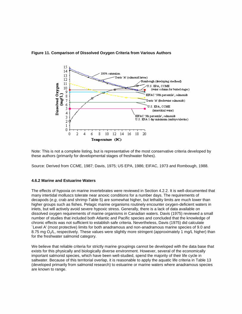
Figure 11. Comparison of Dissolved Oxygen Criteria from Various Authors
Note: This is not a complete listing, but is representative of the most conservative criteria developed by these authors (primarily for developmental stages of freshwater fishes).
Source: Derived from CCME, 1987; Davis, 1975; US EPA, 1986; EIFAC, 1973 and Rombough, 1988.
4.6.2 Marine and Estuarine Waters
The effects of hypoxia on marine invertebrates were reviewed in Section 4.2.2. It is well-documented that many intertidal molluscs tolerate near anoxic conditions for a number days. The requirements of decapods (e.g, crab and shrimp-Table 5) are somewhat higher, but lethality limits are much lower than higher groups such as fishes. Pelagic marine organisms routinely encounter oxygen-deficient waters in inlets, but will actively avoid severe hypoxic stress. Generally, there is a lack of data available on dissolved oxygen requirements of marine organisms in Canadian waters. Davis (1975) reviewed a small number of studies that included both Atlantic and Pacific species and concluded that the knowledge of chronic effects was not sufficient to establish safe criteria. Nevertheless, Davis (1975) did calculate `Level A' (most protective) limits for both anadramous and non-anadramous marine species of 9.0 and 8.75 mg O2/L, respectively. These values were slightly more stringent (approximately 1 mg/L higher) than for the freshwater salmonid category.
We believe that reliable criteria for strictly marine groupings cannot be developed with the data base that exists for this physically and biologically diverse environment. However, several of the economically important salmonid species, which have been well-studied, spend the majority of their life cycle in saltwater. Because of this territorial overlap, it is reasonable to apply the aquatic life criteria in Table 13 (developed primarily from salmonid research) to estuarine or marine waters where anadramous species are known to range.

4.7 Rationale
4.7.1 Cold-Water / Warm-Water Distinction
The US EPA (1986), and subsequently the CCREM (1987) national guidelines, presented separate dissolved oygen guidelines for cold-water (salmonid) and warm-water (non-salmonid) biota to distinguish the different oxygen requirements of these groups. The latter is generally accepted to be less sensitive to hypoxia than salmonids. A group which does not fit well into this categorization is the non-salmonid, cold-water or cool-water fish (e.g., pikes, sculpins). The US EPA (1986) recognized that the oxygen requirements of these species were closer to salmonids, but included them in the derivation of response thresholds for a non-salmonid, warm-water grouping. For the purpose of this document, salmonid and salmonid-like species are considered together and constitute the basis of our criteria for aquatic life.
Understandably, there is a considerable range of oxygen requirements reported for non-salmonids due to the taxonomic and physiological variability of this group. The US EPA (1986) made a qualification that the data base was limited and the need for subjective technical judgement during criteria development was greater. Unlike regions of the United States, salmonid and salmonid-like species are ubiquitous within the cooler waters of British Columbia. Thus, a more stringent criterion for these fish almost always would supersede a need for the application of a non-salmonid or warm-water criterion. For these reasons, and the opportunity for simplification, separate warm-water and cold-water criteria are considered redundant.
4.7.2 Concentration (mg/L) Versus Percent Saturation And Temperature Dependency
Concentration and percent saturation both have been used for specifying a particular level of dissolved oxygen in water. Arguments can be presented for the validity of either expression of criteria, although in recent years there has been a general preference for oxygen concentration in mg/L. Davis (1975) chose percent saturation for his criteria as this was the only value which encompassed both oxygen content and partial pressure at various temperatures. As discussed earlier, Davis considered the oxygen tension gradient between the tissue and external media to be critical for proper gas exchange. At lower temperatures and oxygen solubilities, criteria (in percent saturation) were set to maintain the partial pressure response thesholds that were derived. At higher temperatures, higher percent saturations were necessary to maintain the oxygen content specified in the original response thresholds expressed in mg/L. Several reviewers have disagreed with this premise, notably the IJC (1979), CCREM (1987) and the US EPA (1986), and concluded that a simple criterion in mg/L expressed as a mean and / or minimum was preferable to percent saturation. The main points made in support of this decision are summarized below:
Fish physiology specialists commissioned by the IJC (1980) concluded that the rate of oxygen transfer across fish gills is governed by diffusion down a concentration gradient and is dependent on the mean difference in oxygen partial pressure across the gills. Since the minimal tissue oxygen pressure necessary for normal metabolic activity has not been established, oxygen pressure or percent saturation do not provide a true indication of the pressure differences across the gill. Most of the oxygen can be effectively removed from the water presented to the respiratory surface, therefore it follows that the total amount (concentration) of oxygen delivered to the gills is a more specific limiting factor than is oxygen pressure per se.

Altitude has no known effect on the amount of dissolved oxygen needed by aquatic organisms and there may be no clear choice for either concentration or partial pressure. At a constant percent saturation, the amount of oxygen available decreases with increasing altitude (Chapman, unpublished).
At a constant partial pressure in increasingly saline waters, the concentration will decrease, and a criterion based upon constant partial pressure (or saturation) would unacceptably decrease when expressed as concentration (Chapman, 1994). Note that Davis' (1975) criteria for marine waters, based on percent saturation, are actually higher than comparable freshwater criteria.
There is some indication (e.g., growth effects data) that critical partial pressure of dissolved oxygen probably decreases in cold water. While the concentration would remain the same, percent saturation (and partial pressure) would mandate an increase in the dissolved oxygen concentration and be unnecessarily stringent (IJC, 1979; Chapman, unpublished). The reverse is true in warm water, where the amount of oxygen needed by aquatic life increases, but expressed as partial pressure / saturation, the amount available decreases. Davis (1975) compensated for this by requiring maintenance of higher percent saturations, and corresponding oxygen concentrations, at higher tabulated temperatures (for 15, 20 and 25 degrees C).
The effect of temperature on oxygen response thresholds, in general, has been obvious in some studies (e.g., Rombough, 1988) and absent in others (e.g., Ott, 1980). The effect of temperature on growth of chinook salmon at various dissolved oxygen levels, shown earlier in Figure 7, indicated that high temperatures increased the severity of hypoxia, but had little influence when oxygen levels exceeded 6 mg/L. Davis (1975) included a temperature component in the criteria based on percent saturation; however, Davis oxygen response data (in mg/L) for freshwater fish plotted against test temperatures showed an absence of any relationship. No temperature component is recommended at this time. On the strength of works by Rombough (1988) and expectations of future research in this direction, we recognize that this position could change.
Various formats for expressing dissolved oxygen can convey the same level of protection. However, the added complexity of sliding-scale criteria or some combination of formats (e.g., partial pressure and percent saturation) is considered unnecessary. Furthermore, we accept the generally good `fit' of dissolved oxygen concentration and aquatic life response thresholds within the body of existing research. Dissolved oxygen concentration in mg/L embodies the benefits of a sliding-scale with respect to important environmental variables, in a simpler format, and we believe is an appropriate expression for criteria.
4.7.3 Variable, Minimum and Mean Criteria
Early criteria documents such as Doudoroff and Shumway's (1970) treatise related naturally occurring fluctuations in dissolved oxygen with acceptable seasonal minimums. In their case, the acceptable minimums were offered graphically as multi-levels of protection from no depression of natural conditions (straight-line relationship) through progressively lower protection curves. Selection of the appropriate curve was based upon the value of the fishery, and as such was primarily a socio-economic decision, not a biological one. They specified seasonal minimums as the basis for criteria development, since average oxygen levels would not be protective where wide fluctuations occurred. Regardless of the scientific data utilized to develop the protection threshold(s), a potential shortcoming of seasonally variable criteria is the dependence on sound knowledge of the ambient oxygen regime for each waterbody in question. In addition, human activity may preclude determining of natural minima and the application of this approach.

Some jurisdictions (e.g., CCREM, 1987 and IJC, 1979) have utilized a simple minimum oxygen criterion. Although easy to apply, the natural fluctuations inherent to many dissolved oxygen regimes would result in routine exceedance of conservative criteria set close to saturation. Alternatively, a minimum criterion applied where diurnal cycles are large would not be protective in situations where cycles were minor. Thus, oxygen minima alone can result in under-protection and / or over-protection. The US EPA considered this to be a major shortcoming with their previous single criterion of 5 mg/L (Chapman, unpublished). For example, if the dissolved oxygen concentration is very stable, a 5 mg/L minimum is functionally equivalent to a 5 mg/L average, a level which would cause moderate production impairment to cold-water fish (Table 9). An advisory committee to the IJC (1979) proposed a two-number oxygen criterion: a 6.5 mg/L mean and a 5.5 mg/L minimum; however, this new scheme was never adopted for the Great Lakes. The US EPA (1986) concurred that a simple minimum was too limiting for communicating the complexity of dissolved oxygen requirements and protecting against the effects of hypoxia. In their most recent criteria document, they have utilized a one-day minimum for preventing short-term exposure to potentially lethal low oxygen concentrations, and a mean to provide ongoing protection from chronic effects under sub-optimal conditions.
Chapman (unpublished) explained that in two-number oxygen criteria, the minimum merely puts a `floor' under the operational criteria, that are based on means-where the real protection lies. This is an important concept, as readers should not be overly concerned by what may be first perceived as a low instantaneous threshold. Given that most laboratory research is based on constant exposure testing without regard for natural oxygen flucuation, the application of these data to develop criteria means (rather than minimums) is reasonable. A 30-day mean is a familiar time frame, and the US EPA considered this a sufficient reporting period over which observed effects on growth might be meaningful. They also deemed that a 7-day mean was a necessary averaging period to protect the often short-duration, most sensitive early life stages.
We have adopted two-number (mean / minimum) criteria and a 30-day averaging period for our dissolved oxygen criteria.
4.7.4 The Numerical Criteria
The most recent US EPA (1986) document on dissolved oxygen (cold-water category) is largely based on salmonid species common to British Columbia waters and represents the most authoritative work on the subject thus far. The agency has acknowledged that if their criteria were just maintained for an extended period, there would be risk of production impairment in natural systems, since these are no assured no-effect limits. Rather, the US EPA's conceptual guide has been to protect most species most of the time. The agency also was sensitive to the fact that national criteria often become standards (or objectives) and that socio-economic hardships can result from too-stringent guidelines in the United States. In British Columbia, anthropogenic influences on water quality generally are less and water temperatures are lower; therefore, ambient dissolved oxygen levels can be expected to be higher. We see no justification for compromising protection levels established for dissolved oxygen in this province. The US EPA (1986) also considered this circumstance for other jurisdictions and recommended the `No Production Impairment' values if some assumed risk was unacceptable. Moreover, while criteria must be developed independently without consideration for compounding effects of other potentially harmful constituents, a safety margin is achieved to some degree by selecting conservative limits.
Through the myriad of experimental procedures applied to oxygen deficiency studies, a broad range of response thresholds have been reported. Often, sub-optimal performances are reported in studies of

physiological impacts where short-term effects can be measured. Under the same conditions, the influences on metabolic processes (e.g., feeding, swimming) often are not significant. The approach used here to derive criteria values has been to rely primarily on that portion of the data base that is well-documented and reasonably consistent, and which can most easily be related to the fitness of the organism. We are in agreement with the US EPA (1986) that the effects on fish growth and survival reported at higher oxygen levels and moderate to high seasonal temperatures for the test subjects, provide the best basis for criteria development.
Embryo/Alevin Life Stages -The US EPA considered early life stages to be the least documented for criteria purposes and expressed conservatism in their approach for the following reasons: the potential for exposure to low oxygen triggering simultaneous early hatching with its unknown effect on survival, the apparently significant interaction of slight reductions in dissolved oxygen and high temperature on embryo / alevin survival and the uncertainty of interstitial flow rates (Chapman, unpublished). In addition, early life stages are incapable of an avoidance response to hypoxic conditions or the presence of other stressors. A degree of added conservatism also seems appropriate based on the experience of those who have studied survival in natural or artificial redds (e.g., Sowden and Power, 1985, Coble, 1961; Koski, 1965; Turnpenny and Williams, 1980). The investigators reported lethal oxygen thresholds in the range of 4 to 6 mg/L constant exposure, compared to laboratory studies in which lethality seldom occurred above 3 mg/L. Studies of salmonid redds have shown low instantaneous oxygen minima to occur, which underscores the need for a protective averaging criterion. For early developmental stages, we agree with the US EPA's (1986) rationale for a 5 mg/L, 1- day minimum criterion; however a more conservative 6 mg/L instantaneous minimum has been established for BC This is consistent with the recommended criterion from that agency's own Science Advisory Board (1986), which concluded that greater consideration had to be given to the incomplete (but nonetheless compelling) evidence for chemical interactions and additive stresses likely to be encountered in natural environments. Prolonged exposure at this threshold would result in minor loss of production (6 mg/L is equivalent to the US EPA's 'Slight Production Impairment' level), but is highly unlikely using tiered, two-number criteria. Instantaneous minima in two-number criteria are a recognition that chronic toxicity limits can be safely exceeded for short periods as long as the lower concentration is above that which could result in serious impairment or lethality. As discussed in Section 4.3.3.2 (growth), alevins subjected to short-term hypoxia typically recover fully and achieve normal size. The instantaneous minimum applies to interstitial spawning gravels or the water column where the developmental stages are not buried. In the absence of interstitial data, water column concentrations should be at least 3 mg/L higher (9 mg O2/L) for buried life stages (as explained in Sections 3.3.3).
Several investigators (e.g., Alderdice et al., 1958 and Rombough, 1988) have described the variability in oxygen requirements through the early developmental stages. For practical purposes, a general criterion can only be directed at the most sensitive periods. The criterion which embodies most of the protection for early life stages is the 30-day mean, which limits excursions below the mean over the time period and hence is protective of the short-duration, sensitive stages of development. We have adopted a criterion of 8 mg/L dissolved oxygen (11 mg/L in the water column) for embryo / alevin life stages, primarily based upon the data of Warren et al. (1973) and Silver et al. (1963) contained in Figure 8 (Section 4.3.2.2), which depict growth impairment curves for salmonids subjected to hypoxia. There is a modest inflection point at 8 mg/L corresponding to observed growth reductions that were predominantly below 10 %. In addition, this threshold is above reported responses to hypoxia with respect to time of hatch and first feeding. The US EPA (1986) established a 7-day criterion mean of 6.5 mg/L or 0.5 above their 'Slight Production Impairment' limit. For reasons already stated, we have chosen a more conservative limit which is equivalent to the US EPA 'No Production Impairment' level. While a 30-day

averaging period is less stringent that a 7-day period for a comparable number of sampling events, this should not compromise safety unduly because of the higher threshold being used.
The 8 mg/L threshold can be compared to other criteria that are illustrated in Figure 11. Under Rombough's (1988) proposed scheme for steelhead steelhead trout, for example, 8 mg/L would be in compliance up until interstitial temperatures exceeded 7C.
Juvenile/Adult Life Stages - Again, in two-number criteria an acceptable instantaneous oxygen threshold for aquatic life must avoid severe stress and established lethal limits for the most sensitive species. It was noted earlier that salmonid lethality predominantly has been reported at dissolved oxygen concentrations below 3 mg/L. The US EPA has recognized that a number of riffle-dwelling invertebrates common to salmonid habitats are even less tolerant of acute oxygen deficiency (Chapman, unpublished). The agency considered a 4 mg/L minimum would adequately protect coldwater organisms for a limited duration, but the potential for production impairment at this level was classified as severe. The first part of the British Columbia criteria for juvenile/adult life stages has been set at a more conservative 5 mg/L instantaneous minimum and corresponds to E.P.A.'s 'Moderate Production Impairment' level for salmonids as instantaneous minima (i.e., as an acceptable short-term, non-lethal stress level only-not to be confused with accepting chronic production impairment).
The US EPA (1986) proposed both 7- and 30-day mean criteria of 5 and 6.5 mg/L respectively, for protecting other than early life stages. This added level of complexity was considered unnecessary for the British Columbia situation, as our criterian would be more conservative and the additional monitoring requirements inherent with a 7-day averaging period could be unnecessarily burdensome. The US EPA (1986) acknowledged that mature life stages probably can be adequately protected by a 30-day average. In addition, this time period is more relevant to the observed effects on growth, which have been the basis for development of production impairment levels and criteria. In studies described earlier (Section 4.3.1.2), and particularly those referred to in Figures 7 and 8, growth impairment was negligible above 8 mg/L. An 8 mg/L threshold has been selected as the 30-day mean criterion for juvenile/adult life stages and is the same as the criterion for developmental stages. This is consistent with our use of the US EPA's 'No Production Impairment' values as continuous average thresholds to achieve a high degree of protection.
Relative to other criteria, an 8 mg O2/L limit is approximately equal to Davis' 'Level A' (highest) protection level of 7.75 mg/L for freshwater salmonids, at temperatures of 15C and above (higher oxygen concentrations where specified at lower temperatures). The CCREM (1987) criterion of 6.5 mg O2/L (minimum) could offer a similar degree of protection as our 30-day mean in situations where there is considerable diurnal flucuation in natural oxygen levels. However, as explained in Section 4.7.3, one-number criteria have an inherent inflexibility and can result in under-protection where cycles are minor (i.e., sustained 6.5 mg O2 /L could result in production impairment to aquatic life).
4.8 Application of Criteria
Dissolved oxygen is more reactive and variable in the short-term than most chemical constituents of water. Special considerations are necessary when designing a monitoring program and applying criteria. While it is beyond the scope of this document to develop monitoring protocols, oxygen has some behavioural characteristics that should be recognized.

Oxygen cycles and monitoring frequency - Dissolved oxygen cycles in productive waters are common, and site-specific details must be taken into account when designing a sampling strategy. Diurnal oxygen flucuations typically result in sub-optimal conditions for at least brief periods; therefore, the timing of measurements is very important. It is the intent of two-number criteria, that the lower magnitude of these fluctuations not be less then the criterion for the instantaneous minimum. In natural waters influenced by oxygen generation from primary production, daily cycles usually are sinusoidal with a maximum concentration reached late in the day and a minimum in early morning. Whether a cycle exists naturally or is the result of a manipulated discharge (e.g., a hypolimnetic withdrawal from a reservoir), it is necessary to determine a reasonable average of the extreme high and low concentrations once the shape of the oxygen curve is determined (i.e., a minimum of two measurements must be taken). Cycles are more likely to be non-sinusoidal in manipulated flows, and the US EPA (1986) recommended that time-weighted averages be used in these circumstances. In addition, maximum dissolved oxygen concentrations used in calculating daily averages should not exceed the known saturation limit (Stewart et al. [1967] determined that these elevated levels had no beneficial effect on growth).
The required frequency of sampling can be driven by a number of circumstances (e.g., known variability of oxygen levels in the source water, the most sensitive species / life stages present and their duration, and logistical constraints such as cost or distance between sample sites). For normal ambient monitoring, five measurements taken weekly within 30 days is a minimum (and as mentioned above, daily averages have to be used where cycles exist). Additional sampling is recommended where ambient levels are known to vary over time or are close to criteria values. A few excursions below the mean can easily result in non-compliance. In such cases, additional sampling over a 7-day averaging period would be prudent to check for anomolies and determine the extent of low dissolved oxygen concentrations.
Temperature considerations - It was decided there were insufficient data to incorporate an additional temperature component into broad aquatic life criteria, moreso than is already provided by using single number oxygen concentrations (where corresponding saturation values vary with temperature). We recognize that the effects of hypoxia likely are more severe under the added stress of higher temperatures. If the presence of early life stages (prone to highest mortality) coincides with high seasonal summer temperatures, special attention should be given to the attainment of criteria; however, where the 30-day mean thresholds are likely to be exceeded routinely as a result of natural conditions, site-specific objectives will have to be developed. This would likely be the case for species that spawn in summer such as rainbow trout.
There is some assurance from work by Rombough (1988) that where prevailing water temperatures are less than 7C, criteria thresholds of Table 13 are likely to be overly stringent and could be relaxed for early developmental stages. This opportunity would require adequate knowledge of natural site conditions and could be tempered by the normal variance that is expected for timing of hatch, where oxygen requirements are greatest for early stages (i.e., staggered hatch times could diminish the time 'window' where lower limits apply).
Multiple toxicity considerations - We believe that our dissolved oxygen criteria are sufficiently conservative that multiple toxicity generally will not be cause for concern. With the exception of ammonia, there is limited opportunity in the literature to develop quantitative relationships between dissolved oxygen and potential toxicants. It is recommended that multiple toxicity be dealt with on a site-specific basis where, in the presence of known contaminants (e.g, cyanide, un-ionized ammonia) the criteria for dissolved oxygen and the other contaminants may have to be modified to provide the

appropriate level of protection for aquatic life. Where literature studies lack sufficient detail to accomplish this, bioassasys could be performed on sensitive local species for the range of expected conditions.
Interstitial considerations - It is incumbent on resource managers to have a reasonable understanding of the aquatic life resources being protected. For example, in salmonid-bearing waters, embryos and alevins typically are buried in the stream bottom or shallow lake bed for several months each year. Due to the variety of salmonids endemic to British Columbia, there may only be a limited time that early life stages are not present in spawning media. As discussed previously, the criteria for early life and mature life stages are the same when interstitial measurements are being used for the buried early life stages. If surface water is being tested, a 3 mg/L differential is assumed, wherein the instantaneous minimum and mean criteria values are raised to 8 and 11 mg/L, respectively, for the buried early life stages. Interstitial data clearly represent a more direct and accuarate measure of available oxygen and is preferred; however, the increased complexity of sampling may not be practical for routine field monitoring.
Depth considerations - It should be understood that oxygen concentrations in lakes (particularly in the hypolimnion) and coastal inlets are naturally depressed and cannot be expected to meet the criteria levels herein, which primarily should be applied to surface and near-surface waters. Site-specific objectives could be developed for stratified lakes based on natural historical oxygen concentrations.
General - Natural oxygen levels that do not meet criteria - Studies of dissolved oxygen levels in spawning media have determined that, under some normal circumstances (e.g., summer high temperatures, high elevation, etc.), concentrations may not meet the provincial criteria. Typical survival rates of incubating salmonids from egg deposition through to emergence are known to be relatively low due to a combination of stressors, and lack of oxygen commonly is cited. Based on works such as Rombough (1988), which detail the elevated oxygen requirements near the time of hatch, it is apparent that hypoxic stress, particularly in the interstitial environment, is not uncommon or unnatural during early development.
In cases where natural dissolved oxygen concentrations in surface waters or sub-surface waters do not meet criteria, no statistically significant reduction below natural levels should be permitted. An accurate determination of natural ambient conditions, including temporal variability, would be critical in such an assessment. Statistical comparison of background levels (e.g., for lakes) or upstream / downstream measurements in relation to a perturbation such as a discharge should use a one-tailed, two sample t-test, at the 0.05 probability level. The minimum sampling requirement is five measurements collected weekly in 30 days. The two sample t-test requires the different stations to have similar variances (use the F-test). If, at the affected site, data from a discharge event are pooled with steady-state data, the variance may increase and become dissimilar to the ambient site, invalidating the two sample t-test. To reduce the variance, data from the steady state and the event should be treated independently.

Table 13. Provincial Dissolved Oxygen Criteria for Aquatic Life for Fresh, Marine and Estuarine Waters, and Sediments
All Life Stages other than Buried Embryos/Alevins
Buried Embryo/Alevin Life Stages
1
Water Column (mg O2 /L)
Water Column2
(mg O2 /L) Interstitial (mg O2/L)
30-day mean3 8 11 8
Instantaneous minimum
4
5 9 6
1 Instream concentrations from spawning to the point of yolk sac absorption or 30 days post-hatch for
fish. 2 Water column concentrations recommended to achieve interstitial dissolved oxygen values when the
latter are unavailable. Interstitial oxygen measurements would supercede water column data. 3 Based on at least 5 approximately evenly spaced samples in 30 days. If a diurnal cycle exists,
measurements should be taken when oxygen levels are low (usually early morning). 4 Minimum level to be maintained at all times.
Source: Derived in part from US EPA, 1986
5.0 Other Water Uses
5.1 Drinking Water
There are both positive and negative attributes of having dissolved oxygen in domestic drinking water. While corrosion within older cast iron water supply systems is a result of oxidative processes, the effects of oxygen are mostly beneficial. Dissolved oxygen prevents the chemical reaction and leaching of iron and manganese from the sediments in source water, which otherwise would stain plumbing fixtures and cause taste problems. It facilitates the biochemical oxidation of ammonia to nitrate, reduces the chlorine demand of waters and increases the disinfection efficiency of chlorination (NAS/NAE, 1972). Also, a high level of dissolved oxygen is generally considered more palatable in water, as opposed to there being a 'flat' taste.
Dissolved oxygen criteria for drinking water which exist in adjacent jurisdictions include: 5 mg/L minimum-same as for aquatic life (Alberta Environment, 1977), >8.0->9.5 mg/L-same as for aquatic life (State of Washington, 1982) and 4 mg/L (Alaska, 1979). Public drinking water supplies in British Columbia are generally well-oxygenated and an additional criterion for this category is not considered necessary at this time.
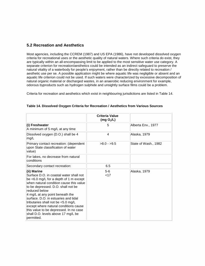
5.2 Recreation and Aesthetics
Most agencies, including the CCREM (1987) and US EPA (1986), have not developed dissolved oxygen criteria for recreational uses or the aesthetic quality of natural waters. Where such criteria do exist, they are typically within an all-encompassing limit to be applied to the most sensitive water use category. A separate criterion for recreation/aesthetics could be intended as an indirect safeguard to preserve the natural vitality of a waterbody for people's enjoyment, rather than be directly related to recreation / aesthetic use per se. A possible application might be where aquatic life was negligible or absent and an aquatic life criterion could not be used. If such waters were characterized by excessive decomposition of natural organic material or discharged wastes, in an anaerobic reducing environment for example, odorous byproducts such as hydrogen sulphide and unsightly surface films could be a problem.
Criteria for recreation and aesthetics which exist in neighbouring jurisdictions are listed in Table 14.
Table 14. Dissolved Oxygen Criteria for Recreation / Aesthetics from Various Sources
Criteria Value (mg O2/L)
(i) Freshwater A minimum of 5 mg/L at any time
5 Alberta Env., 1977
Dissolved oxygen (D.O.) shall be 4 mg/L
4 Alaska, 1979
Primary contact recreation: (dependent upon State classification of water value)
>8.0 - >9.5 State of Wash., 1982
For lakes, no decrease from natural conditions
Secondary contact recreation: 6.5
(ii) Marine Surface D.O. in coastal water shall not be <6.0 mg/L for a depth of 1 m except when natural condition cause this value to be depressed. D.O. shall not be reduced below 4 mg/L at any point beneath the surface. D.O. in estuaries and tidal tributaries shall not be <5.0 mg/L except where natural conditions cause this value to be depressed. In no case shall D.O. levels above 17 mg/L be permitted.
5-6 <17
Alaska, 1979

Criteria Value (mg O2/L)
Primary contact recreation: D.O. shall exceed 6.0 or 7.0 mg/L depending upon the classification. When natural conditions such as upwelling occur, causing the D.O. to be depressed near or below these levels, natural D.O. levels can be degraded up to 0.2 mg/L by man-caused activities.
>6.0 - >7.0 State of Wash., 1982
Secondary contact recreation: D.O. shall exceed 4.0 or 5.0 mg/L depending upon the classification (and as above).
>4.0->5.0
Dissolved oxygen criteria for recreation and aesthetics are not deemed necessary for British Columbia, as the criteria for aquatic life can be protective of virtually all waters implicated in these use categories.
5.3 Industry
5.3.1 Effects
With the exception of the food and beverage industries (using production water) and aquaculture, the presence of natural levels of dissolved oxygen in water for industrial operations generally is undesirable for the following reasons:
i. Oxygen increases corrosion in metal pipes and related equipment, particularly in heating (boilers) and cooling systems. In a packaged power reactor, dissolved oxygen can cause stress corrosion of stainless steel (McKee and Wolfe, 1963). These corrosive effects increase substantially in the presence of low pH.
ii. Oxygen promotes slime-forming organisms and deposits, and interferes with paper fibre retention in pulp and paper processing (CCREM, 1987). Dissolved oxygen reduces hydrogen bonding between fibres, which can cause imbalance of clays and fines in pulping stock (Schmok, 1992).
5.3.2 Criteria from the Literature
Water quality requirements of industries are as varied as the products they produce and it is not within the scope of this report to identify specific dissolved oxygen criteria except those generally quoted for

generic uses. It is accepted that industries incorporate conditioning processes to provide the quality levels necessary. Common additives to remove oxygen are sulphites and hydrazine.
The pulp and paper industry is the largest industrial process water user in British Columbia. On an industry-wide basis in Canada, the major use categories are cooling, condensing and steam generation (CCREM, 1987).
Table 15 contains a listing of the more common guidelines for dissolved oxygen in major industries. Since the low concentrations of dissolved oxygen necessary for industry have little relation to natural levels and must be attained by internal scavenging processes, no criteria for intake water are proposed. In the specific case of food processing water, which typically has some minimum dissolved oxygen requirement, the aquatic life criteria established in Section 4 would be adequate for this use. Similarly, oxygen requirements for the aquaculture industry (marine and freshwater) should be adequately met by the aquatic life criteria herein. As the level of survival success under natural conditions is not acceptable to fish hatchery operators, incubation systems attempt to optimize physical variables such as oxygen and temperature throughout development. These requirements do not fall within the scope of ambient criteria. Models such as that of Rombough (1986) have been prepared on the oxygen requirements of hatchery fish, and some of the references cited earlier cover this subject (e.g., SIGMA, 1983 and Rombough, 1988).
Table 15. Dissolved Oxygen Criteria for Industry from Various Sources
Criteria statement Criteria Value (mg o2/L)
Reference
(i) Freshwater Levels should not exceed 0.03 mg O2/L to prevent stress corrosion of stainless steel in packaged power reactors
0.03 McKee and Wolfe, 1963
Levels for boiler feed water not to exceed: 2 mg O2/L for 0-1.03 M Pa; 0.2 mg O2/L for 1.03-1.72 M Pa; and 0.0 mg O2/L for >1.72 M Pa
2.0 0.2 0.0
(depending on pressure)
McKee and Wolfe, 1963
Some industrial uses 4.0 DOE, 1972
Maximum levels for feedwater at the following operating pressures:low (0-1.03 M Pa) 2.5 mg O2/L, moderate (1.03-4.83 M Pa) 0.007 mg O2/L and high (4.83-10.34) 0.007 mg O2/L. For electrical utilities (pressure between 10.34-34.48 M Pa) 0.007 mg O2/L
2.5 (boiler) 0.007
(depending on pressure)
NAS/NAE, 1972
Minimum to maintain aerobic conditions at point of use for the iron and steel industry
aerobic NAS/NAE,1972 CCME, 1987
Industrial uses (other than food processing) -no detrimental effects on established water supply treatment levels
Alaska, 1979
Industrial uses (other than food processing) 3.0 Montana, 1980

Criteria statement Criteria Value (mg o2/L)
Reference
Industrial water 4.0 State of Wash., 1982
Levels to be less than the following for feedwater incurrent design industrial steam generators-assumes the pressure of a deaerator but measured before chemical oxygen scavenging: Industrial Watertube 0-3.1 M Pa: 0.04 mg O2/L 3.11-13.7 M Pa: 0.007 mg O2/L Industrial Firetube w/o Superheater 0-2.07 M Pa: 0.04 mg O2/L Industrial Coil-Type Watertube 0-4.14 M Pa: 0.2 mgO2/L >4.14 M Pa: 0.007 mg O2/L
0.2 0.04 0.007
(depending on pressure)
CCME, 1987
(ii) Marine Seafood processing
>5 Alaska, 1979
6.0 Research and Development Needs
Temperature It is accepted that chronic toxicity (e.g., growth impairment) from hypoxia is negatively affected at higher temperatures. However, there continues to be sufficient controversy, and inconsistency or lack of data, that additional studies are needed. The majority of researchers have employed a safety factor when deriving dissolved oxygen requirements by utilizing high seasonal temperatures for the organisms under study. Rombough's (1988) work shows promise that a temperature component of oxygen criteria eventually may be possible for individual species and taxonomic groupings. In addition, few studies employ cold-water test conditions (the other extreme, where criteria are potentially over-protective); further work in this area would be helpful.
Oxygen cycles Typical dissolved oxygen research reflects controlled conditions with constant exposure levels over relatively short time periods. More work is required on the effects of naturally flucuating dissolved oxygen levels (it is known, for example, that the reduced growth rate of fish during the depressed period of a sinusoidal oxygen cycle is not compensated for during the elevated period). While there is limited information on the effects of daily oxygen cycles, there is even less known about irregular oxygen cycles as may occur below controlled discharges from an impoundment.
Interstitial oxygen The assumed 3 mg O2/L differential between surface water and interstitial water, adopted by the US EPA (1986) and used in our own criteria, is based on only two studies of natural redds. Additional effort is required to further test the validity of this assumption. It may be that the magnitude of variability could

preclude the use of a standard differential and that more efficient methods of monitoring oxygen within the streambed are needed.
Narrow data The literature base on dissolved oxygen research is heavily biased to the few economically important salmonid species. Investigation needs to be expanded within groupings such as freshwater invertebrates and marine species.
7.0 References Cited
Adelman, I.R., and L.L. Smith. 1972. Effect of oxygen on growth and food conversion efficiency of northern pike. Prog. Fish-Cult. 32: 93-96.
Alaska Department of Environment Conservation. 1979. Water Quality Standards. Alaska Water Pollution Control Program. Juneau, Alaska.
Alberta Environment. 1977. Alberta Surface Water Quality Objectives. Water Quality Branch, Standards and Approvals Division. 17p.
Alderdice, D.F., W.P. Wickett and J.R. Brett. 1958. Some effects of temporary exposure to low dissolved oxygen levels on pacific salmon eggs. J. Fish. Res. Board Canada 15: 229-250.
Alabaster, J.S. 1989. The dissolved oxygen and temperature requirements of king salmon (Oncorhyncus tshawytscha) in the San Joaquin Delta, California. J. Fish. Biol. 34: 331-332.
Alabaster, J.S. 1988. The dissolved oxygen requirements of upstream migrant chinook salmon, Oncorhynchus tshawytscha, in the lower Willamette River, Oregon. J. Fish. Biol. 32: 635-636.
Alabaster, J.S., O.W.M. Herbert, and J. Hemens. 1957. the survival of rainbow trout (Salmo gairdnerii richardson) and perch (Perca fluviatilis l.) at various concentrations of oxygen and carbon dioxide. Ann. of Appl. Biol. 45 (1): 177-188.
Alabaster, J.S. and R. Lloyd. 1982. Water Quality Criteria for Freshwater Fish. 2nd Edition. Food and Agriculture Organization of the United Nations. Butterworth's, London. 361 p.
Alderdice, D.F. and J.R. Brett. 1957. Some effects of kraft mill effluent on young pacific salmon. J. Fish. Res. Board Canada 14: 783-795. (Cited In: McLeay and Assoc., 1986).
(American Public Health Association). 1992. Standard Methods for the Examination of Water and Wastewater. 18th ed. American Public Health Association, Washington, D.C.
Anon. 1974. Kalamalka-Wood Lake Basin Water Resource Management Study, Water Resources Service, Ministry of Environment, Victoria, BC 209 p.
Birtwell, J.K. 1989. Comments on the sensitivity of salmonids to reduced levels of dissolved oxygen and to pulp mill pollution in Neroutsos Inlet, BC Can. Tech. Rep. Fish. Aquat. Sci. 1695: 27 p.

Birtwell, J.K. and G.M. Kruzynski. 1989. In situ and laboratory studies on the behaviour and survival of pacific salmon. (genus Oncorhyncus). In: Environmental bioassay techniques and their apparatus. M. Munawar, G. Dixon, C.I. Mayfield, T. Reynoldson and M.H. Sadar, (eds.). Hydrobiologia. Kluwer Academic Pub., The Netherlands.
Brannon, E.L. 1965. The Influence of Physical Factors on The Development and Weight of Sockeye Salmon Embryos and Alevins. International Pacific Salmon Fisheries Commission. Progress Rep.No. 12. New Westminster, BC 26 p.
Brett. J.R. 1979. Bioenergetics and Growth. Vol. VIII. In: Fish Physiology. Academic Press. New York, N.Y.
Brett, J.R. and J.M. Blackburn. 1981. Oxygen requirements for growth of young coho salmon (Oncorynchus kisutch) and sockeye salmon (O. nerka) at 15C. Can. J. Fish. Aquat. Sci. 38: 399-404.
Brinkman, A.G., W. van Raaphorst and L. Lijklema. 1982. In situ sampling of interstitial water from lake sediments. Hydrobiologia 92: 659-663.
Broderius, S.J. 1970. Determination of Molecular Hydrocyanic Acid in Water and Studies of the Chemistry and Toxicity to Fish of the Nickelo-cyanide complex. M.S. Thesis. Orgeon State University, Corvallis. 93 p.
Brook, L.T. and P.J. Colby. 1980. Development and survival of embryos of lake herring at different constant oxygen concentrations and temperatures. Prog. Fish-Cult. 42: 3-9.
Bryan, J.E. 1990. Water Quality of Okanagan, Kalamalka and Wood Lakes. BC Environment, Technical Report. ISBN 0-7726-1182-3.
Bushnell, P.G., J.F. Steffensen and K. Johansen. 1984. Oxygen consumption and swimming performance in hypoxia-acclimated rainbow trout (Salmo gairdnerii). J. Exp. Biol. 113: 225-235.
Cairns, J. Jr. and A. Scheier. 1958. The Effect of Periodic Low Oxygen Upon Toxicity of Various Chemicals to Aquatic Organisms. Proc. 12th Ind. Waste Conf. Purdue Univ., Eng. Ext. Ser. No. 94 Eng. Bull. 42: 165 (Cited In: Singleton, 1986).
Canada-British Columbia Okanagan Basin Agreement (BCOBA). 1974. The Limnology of the Major Okanagan Basin Lakes: Technical Supplement V to the Final Report. Office of the Study Director. Penticton, BC 271 p.
CCREM (Canadian Council of Resource and Environment Ministers - now the CCME - Canadian Council of Ministers for the Environment). 1987. Canadian Water Quality Guidelines. Task Force on Water Quality Guidelines of the Canadian Council of Resource and Environment Ministers. 256 p.
Carlson, A.R. and R.E. Siefert. 1974. Effects of reduced oxygen on the embryos and larvae of lake trout (Salvelinus namaycush) andlargemouth bass (Micropterus salmoides). J. Fish. Res. Board Canada. 31:1393-1396.

Chapman, G.A. Unpublished. Response to Public Comment-Dissolved Oxygen Criteria. US EPA. 63 p.
Chapman, G.A. 1969. Toxicity of Pentachlorophenol to Trout Alevins Ph.D. Thesis. Oregon State University. Cowallis, Oregon. 87 p.
Chapman, G.A. and D.L. Shumway. 1978. Effects of Sodium Penlachlorophenate on Survival and Energy Metabolism of Embryonic and Larval Steelhead Trout. In: Pentachlorophenol-Chemistry, Pharmacology, and Environmental Toxicology Proceedings of a symposium in Pensacola, Florida. June, 1977. p. 285-299.
Chevalier, B.E. and C. Carson. 1985. Modelling the Transfer of Oxygen Between the Stream and Stream Substrate with Application to the Survival Rates of Salmonid Embryos. Colorado State Univ., Dept. Ag. Chem. Eng., ARS Proj. No. 5602-20813-008A. 99 p.
Chevalier, B.E. and V.G. Murphy. 1985. Intragravel Dissolved Oxygen Model. Colorado State Univ., Dept. Ag. Chew. Eng., ARS CWV No. 5402-20810-004-015. 68 p.
Childress, J.J. 1971. Respiratory adaptations to the oxygen minimum layer in the bathypelagic myoid gnathophausia intens. Univ. of Calif.Biol. Bull. 141: 109-121.
Coble, D.W. 1961. Influence of water exchange and dissolved oxygen in the redds on survival of steelhead trout embryos. Trans. Am. Fish. Soc. 90: 469-474.
Colt, J. 1984. Computation of Dissolved Gas Concentrations in Water as Functions of Temperature and Salinity and Pressure. American Fisheries Society Spec. Pub. 14, Bethesda, MD. 81 p.
Cook, G.D., E.B. Welch, P.A Spence, and P.R. Newroth. 1986. Lake and Reservoir Restoration. Butterworth Publishers, Stoucham, MA. 392 p.
Dahlberg, M.L., D.L. Shumway and P. Doudoroff. 1968. Influence of dissolved oxygen and carbon dioxide on swimming performance of largemouth bass and coho salmon. J. Fish. Res. Board Canada 25: 49-70.
Davis, G.E., J. Foster, C.E. Warren and P. Doudoroff. 1963. The influence of oxygen concentration on swimming performance of juvenile pacific salmon at various temperatures. Trans. Am. Fish. Soc. 92: 111-124.
Davis, J.C. 1975. Waterborne Dissolved Oxygen Requirements and Criteria with Particular Emphasis on the Canadian Environment. National Research Council of Canada. Associate Committee on Scientific Criteria for Environmental Quality, NRCC No. 14100. 111 p.
Davison, R.C., W.P. Breese, C.E. Warren, and P. Doudoroff. 1959. Experiments on the Dissolved Oxygen Requirements of Cold-water Fishes. Sewage Incl. Wastes 31: 950-966. (Cited In: Warren et al., 1973).
Department of Environment (DOE). 1972. Guidelines for Water Quality Objectives and Standards. Technical Bulletin No. 67. Inland Waters Branch, Department of Environment. Ottawa, Canada.

Dorfman, D. and W. R. Whitworth. 1969. Effects of lead, temperature and dissolved oxygen on the growth of the brook trout. J. Fish. Res. Board Canada 26: 2493-2501.
Doudoroff, P. and D.L. Shumway. 1970. Dissolved Oxygen Requirements of Freshwater Fishes. Food and Agriculture Organization of the United Nations. FAO Tech. Paper 86. 291 p.
Downing, K.M. 1954. The influence of dissolved oxygen concentration on the toxicity of potassium cyanide to rainbow trout. J. Exp. Biol. 31: 161-164.
Downing, K.M. and J.C. Merkens. 1957. The influence of temperature on the survival of several species of fish in low tensions of dissolved oxygen. An. Appl. Biol. 45 (2): 261-267.
Drinnan, R.W. and M.J.R. Clark. 1980. Fraser River Estuary Study: Water Chemistry 1970-1978. Government of Canada and Province of British Columbia, Ministry of Environment and Parks, Victoria, BC 160 p.
Eddy, R.M. 1972. The Influence of Dissolved Oxygen Concentrations and Temperature on the Survival and Growth of Chinook SalmonEmbryos and Fry. M.S. Thesis. Oregon State University, Corvallis. 45 p. (Cited In: US EPA, 1986).
ENVIROCON LTD. 1981. Kemano Completion: Hydroelectric Development Baseline Environmental Studies. Vol. 2. Physical and Hydrological Studies. Prepared for: Aluminum Company of Canada Ltd. (Draft) 389 p.
European Inland Fisheries Advisory Commission (EIFAC). 1973. Water Quality Criteria for European Freshwater Fish. Report on Dissolved Oxygen and Inland Fisheries. EIFAC Tech. Paper No. 86.
Fisher, R.J. 1963. Influence of Oxygen Concentration and its Diurnal Fluctuation on the Growth of Juvenile Coho Salmon. M.S. Thesis. Oregon State University, Corvallis. 48 p. (Cited In: US EPA, 1986).
Frodge, J.D., G.L. Thomas and G.B. Paulex. 1990. Effects of canopy formation by floating and submergent aquatic macrophytes on the water quality of two shallow pacific northwest lakes. Aquat. Bot. 38: 231-248.
Fry, F.E.J. 1957. The Aquatic Respiration of Fish. p. 1-63. In: M.E. Brown (ed.). The Physiology of Fishes. Vol. 1. Academic Press Inc. New York. N.Y.
Garside, E.T. 1959. Some effects of oxygen in relation to temperature on the development of lake trout embryos. Can. J. Zool. 37: 689-698.
Garside, E.T. 1965. Effects of oxygen in relation to temperature on the development of embryos of brook trout and rainbow trout. J. Fish. Res. Board Canada 23(8):1121-1134.
Gaufin, A.R. 1973. Water Quality Requirements of Aquatic Insects. EPA 660/3-73-004. US EPA Corvallis, OR. (Cited In: Nebeker et al., 1992).

Gee, J.H., R.F. Tallman and H.J. Smart. 1978. Reactions of some plains fish to progressive hypoxia. Can. J. Zool. 56: 1962-1966.
Gottwald, S. 1965. Der einfluss zeitweiligen saverstoffmangels in verschiedenen stadien auf die embryonalentwicklung der regenbogenforelle (Salmo gairdner: Rich.) Z. Finch. 13 (1/2): 63-84. (Cited In:: Doudoroff and Shumway, 1970).
Gross, M.G. 1972. Oceanography: A View of the Earth. Prentice-Hall Inc. New Jersey. 581 p.
Harrison, P.J., J.D. Fulton, J.J.R. Taylor and T.R. Parsons. 1983. Review of the biological oceanography of the Strait of Georgia: pelagic environment. Can. J. Fish. Aquat. Sci. 40: 1064-1094.
Heier, S. 1991. Manager, Client Liaison. Zenon Environmental Laboratories. Vancouver, BC Personal Communication.
Hermann, R.B., C.E. Warren, and P. Doudoroff. 1962. Influence of oxygen concentration on the growth of juvenile coho salmon. Trans. Am. Fish. Soc. 91: 155-167.
Hicks, D.B. and J.W. Dewitt. 1971. Effects of dissolved oxygen on kraft pulp mill effluent toxicity. Water Res. 5: 693-701. (Cited In: McLeay and Assoc., 1986).
Hitchman, M.L.. 1978. Measurement of Dissolved Oxygen. John Wiley and Sons, New York. 255 p.
Hollender, B.A. 1981. Embryo Survival, Substrate Composition and Dissolved Oxygen in Redds of Wild Brook Trout. University of Wisconsin, Stevens Point. 87 p.
Holm, T.R., George G.K. and M.J. Barcelona. 1986. Dissolved Oxygen and Oxidation-Reduction Potentials in Ground Water. EPA 600:52-86:042, Washington, D.C.
Homer, D.H. and W.T. Waller. 1983. Chronic effects of reduced dissolved oxygen on Daphnia magna. Water Air Soil Pollut. 20: 23-28. (Cited In: Nebeker et al., 1992).
Hoos, R.A.W. 1970. Distribution and Physiology of Zooplankton in an Oxygen Minimum Layer. M.Sc. dissertation, University of Victoria, BC 113 p. (Cited In: Davis, 1975).
Hoos, L.M. 1973. A Study of the Benthos of an Anoxic Marine Basin and Factors Affecting its Distribution. M.Sc. thesis, Dalhousie Univ., NovaScotia. 149 p. (Cited In: Davis, 1975).
Huddard, R. and D.R. Arthur. 1971. Shrimps in relation to oxygen depletion and its ecological significance in a polluted estuary. Environmental Pollution 2:13-35. (Cited In: Davis, 1975).
International Joint Commission (IJC). 1979. Report of the Review Committee for the Dissolved Oxygen Objective for the Great Lakes. Great Lakes Science Advisory Board. Windsor, Ontario.
International Joint Commission (IJC). 1980. Report of the Aquatic Ecosystem Objectives Committee. Great Lakes Science Advisory Board. Windsor, Ontario.

Jensen, E.V. 1981. Results of the Continuing Water Quality Monitoring Program on Okanagan Lakes for Years 1979 to 1980. For: Canada-British Columbia Okanagan Basin Implementation Agreement. Ministry of Environment, Waste Management Br. 73 p.
Jones, D.R. 1971. The effect of hypoxia and anemia on the swimming performance of rainbow trout (Salmo gairdnerii). J. Exp. Biol. 55: 541-551.
Kay, B.H. 1986. West Coast Marine Environmental Quality: Technical Reviews. Environmental Protection Services. Reg. Prog. Rep. 86-01, 154 p.
Koski, K. V. 1965. The Survival of Coho Salmon (Oncorhynchus kisutch) from Egg Deposition to Emergence in Three Oregon Coastal Streams. Oregon State University, Corvallis. 81 p.
Koski, K.V. 1975. The Survival and Fitness of Two Stocks of Chum Salmon (Oncoryhnchus keta) From Egg Deposition to Emergence in a Controlled Stream Environment at Big Beef Creek. Doctoral Thesis. Univ. of Wash. 212 p.
Katz, M., A. Pritchard and C.E. Warren. 1959. Ability of some salmonids and a centrarchid to swim in water of reduced oxygen content. Trans. Am. Fish. Soc. 88: 88-95.
Kruzynski, G.M. Unpublished Data. (Cited In: Birtwell, 1989).
Leduc, G., R.C. Pierce and I.R. McCracken. 1982. The Effects of Cyanides on Aquatic Organisms with Emphasis Upon Freshwater Fishes. National Research Council Canada No. 19246. Associate Committee on Scientific Criteria for Environmental Quality. Ottawa (Cited from Singleton, 1986).
Leppink, J.D. and J. Valentine. 1989. Oxygen injection: its use for water quality improvement and growth enhancement for raceway culture of rainbow trout. Aquaculture Today, p. 35-36.
Levings, C.D. 1972. (Unpublished Data) Cruise Report-June, September and November, 1972. (Cited In: Davis, 1975).
Levings, C.D. and N.G. McDaniel. 1974. A Unique Collection of Baseline Biological Data: Benthic Invertebrates from an Underwater Cable Across the Strait of Georgia. J. Fish. Res. Board Canada, Tech. Rep. 441. 10p. (Cited In: Davis, 1975).
Lewin, R. A. 1962. Physiology and Biochemistry of Algae. New York, New York. Academic Press. 929 p.
Lloyd, R. 1961. Effect of dissolved oxygen concentration on the toxicity of several poisons to rainbow trout (Salmo gairdnerii Richardson). J. Exp. Biol. 38: 447-455. (Cited In: US EPA, 1986).
McGreer, E.R. and G.A. Vigers. 1983. Development and Validation of an In Situ Fish Preference-Avoidance Technique for Environmental Monitoring of Pulp Mill Effluents. p. 519-529. In: Aquatic Toxicology and Hazard Assessment: Sixth Symposium, ASTM STP 802. W.E. Bishop, R.D.Cardwell and BC Heidolph, (eds.), ASTM, Philadelphia. 519-529.

McKee, J.E. and H.W. Wolf. 1963. Water Quality Criteria. Second Ed., California State Water Res. Contr. Bd. Publication No. 3-A, 548 p.
McLean, W.E. (unpublished) 1988. Impact of Sediment on a Chum Salmon Spawning Channel. Presented at Water Quality Objectives Workshop. Nov. 1988. Vanc. BC 8 p.
McLeay, D. and Assoc. 1986. Aquatic Toxicity of Pulp and Paper Mill Effluents: A Review. 243 p.
MacLeod, J.C. and L.L. Smith, Jr. 1966. Effect of pulpwood fibre on oxygen consumption and swimming endurance of the flathead minnow, Pimephales promelas. Trans. Am. Fish. Soc. 95(1): 71-84.
McNeely, R.N., Neimanis, V.P. and L. Dwyer. 1979. Dissolved Oxygen. In: Water Quality Sourcebook. A Guide to Water Quality Parameters. Water Quality Branch, Inland Waters Directorate, Environment Canada, Ottawa, Ont. pp. 33-34.
McNeil, W.J. 1956. The Influence of Carbon Dioxide and pH on the Dissolved Oxygen Requirements of Some Freshwater Fish. M.S. Thesis. Oregon State University, Corvallis. (Cited In: Warren et al., 1973).
McNeil, W.J. 1962. Variations in the Dissolved Oxygen Content of Intergravel Water in Four Spawning Streams of Southeastern Alaska. USDA Fish Wildl. Serv. Spec. Sci. Rep. No. 402. 20 p.
Magnuson, J.J. and D.J. Karlen. 1970. Visual observation of fish beneath the ice in a winterkill lake. J. Fish. Res. Board Canada 27: 1059-1068.
Mason, J.C. 1969. Hypoxial stress prior to emergence and competition among coho salmon fry. J. Res. Bd. Can. 26 (1): 63-91.
Montana Health and Environmental Sciences. 1980. Water Quality. Administration Rules 16.20.616 to 16.20.624 of Montana.
Morris, S. and A.J. Leaney. 1980. The Somass River Estuary: Status of Environmental Knowledge to 1980. Fisheries and Oceans Canada and Environment Canada. Special Estuary Series No. 9. 374 p.
Moss, B. 1980. Ecology of Fresh Waters. John Wiley and Sons Inc. New York. 332 p.
NAQUADAT. 1985. National Water Quality Data Bank. Water Quality Branch, Inland Waters Directorate, Environment Canada, Ottawa. (Cited In: CCME, 1987).
National Academy of Science / National Academy of Engineering (NAS/NAE). 1972. Water Quality Criteria. A Report of Committee on Water Quality Criteria. Washington, D.C. 594 p.
NCASI (National Council of the Paper Industry for Air and Stream Improvement Inc.). 1985. A Literature Review of the Possible Effects of Gas Supersaturation on Aquatic Organisms. National Council of the Paper Industry for Air and Stream Improvement Inc. Tech. Bull. No. 476. New York, N.Y. 25 p.
Nebeker, A.V. 1972. Effects of low oxygen concentration on survival and emergence of aquatic insects. Trans. Am. Fish. Soc. 101: 675-679.

Nebeker, A.V., S.T. Onjukka, D.G. Stevens, G.A. Chapman and S.E. Dominguez. 1992. Effects of low dissolved oxygen on survival, growth and reproduction of Daphnia, Hyalella and Gammarus. Environmental Toxicology and Chemistry, 11(3):373-379.
Ott, M.E., N. Heigler and G.R. Ultsch. 1980. A re-evaluation of the relationship between temperature and the critical oxygen tension in freshwater fishes. Comp. Biochem Physiol. Vol 67 A: 337-340. (Cited In: SIGMA, 1983)
Parasada Rao, D.G.V. and Ganapati, P.N. 1968. Respiration as a function of oxygen concentration in intertidal barnacles. Mar. Biol. 1:309-310.
Parker, R.R. and J. Sibert. 1972. Effects of Pulpmill Effluent on The Dissolved Oxygen Supply in Alberni Inlet, British Columbia, Fish. Res. Bd. Can. Tech. Rept. No. 316. Pacific Biological Station, Nanaimo, BC 41 p. (Cited in: Morris and Leaney, 1980).
Peterka, J.J. and J.S. Kent. 1976. Dissolved Oxygen, Temperature and Survival of Young at Fish Spawning Sites. Environmental Protection Agency Report No. EPA-600/3-76-113, Ecological Research Series. 36 p. (Cited In: US EPA, 1986).
Petrsosky, B.R. and J.J. Magnuson. 1973. Behavioural Responses of Northern Pike, Yellow Perch and Bluegill to Oxygen Concentrations Under Simulated Winterkill Conditions. Copy, No. 1: 124-133
Pickard, G.L. 1961. Oceanic features of inlets in the British Columbia Mainland Coast. J. Fish. Res. Board Canada 18: 907-999.
Pickard, G.L. 1963. Oceanic characteristics of inlets of Vancouver Island, British Columbia. J. Fish. Res. Board Canada 20: 1109-1144.
Pyper, J and E.H. Vernon (Ms-unpublished). 1955. Physical and Biological Features of Natural and Artificial Spawning Grounds of Fraser River Sockeye. Int. Pac. Sal. Fish. Comm., 98 p. (Cited In: Servizi et al., 1970).
Ramsey, W.L. 1962. Bubble Growth from Dissolved Oxygen Near the Sea Surface. Limnol. Oceanog. 7 1-7. (Cited In: Wetzel, 1983).
Reynolds, C.S. 1984. Ecology of Freshwater Phytoplankton. Cambridge University Press. 384 p.
Rombough, P.J. 1986. Mathematical model for predicting the dissolved oxygen requirements of steelhead (Salmo gairdneri) embryos and alevins in hatchery incubators. Aquaculture, 59:119-137.
Rombough, P.J. 1988. Growth, aerobic metabolism, and dissolved oxygen requirements of embryos and alevins of steelhead, Salmo gairdneri. Can. J. Zool. 66: 651-660.
Sassaman, C. and Mangum, C.P. 1972. Adaptations to environmental oxygen levels in infaunal and epifaunal sea anemones. Biol. Bull.143:657-678.
Schmok, M. 1992. Personal communication. Process Engineer, Island Paper.

Science Advisory Board. 1986. A Review of the Agency's Ambient Water Quality Criteria Document for Dissolved Oxygen - Fresh Water Aquatic Life. EPA. SAB-EET&FC-86-020. 28p.
Scrivener, J.C. and M.J. Brownlee. 1980. A Preliminary Analysis of Carnation Creek Gravel Quality Data, 1973-1980. In: Proceedings from the Conference: "Salmon Spawning Gravel: a Renewable Resource in the Pacific Northwest?" Seattle, Washington. p. 195-226.
Scrivener, J.C. and M.J. Brownlee. 1989. Effects of forest harvesting on spawning gravel quality and on incubation survival of chum (Oncorhyncus keta) and coho salmon (O. kisutch) in Carnation Creek, British Columbia. Dept. of Fish and Oceans.J. Fish. Aquat. Sci. Vol. 46.
Sculthorpe, C.D. 1967. The Biology of Vascular Plants, Edward Arnold Ltd. London. 610 p.
Siefert, R.E., A.R. Carlson and L.J. Herman. 1974. Effects of reduced oxygen concentrations on the early life stages of mountain whitefish, smallmouth bass and white bass. Prog. Fish-Cult. 36: 186-190.
Siefert, R.E., W.A. Spoor and R.F. Syrett. 1973. Effects of reduced oxygen concentrations on northern pike (Esox lucius) embryos and larvae. J. Fish. Res. Board Canada 30: 849-852.
Siefert, R.E. and W.A. Spoor. 1974. Effects of Reduced Oxygen on Embryos and Larvae of the White Sucker, Coho Salmon, Brook Trout and Walleye. p. 487-495. In: J.H.S. Blaxter (ed). The Early Life History of Fish. The Proceedings of an International Symposium. Oban, Scotland. May 17-23, 1973. Springer-Verlag, Berlin.
Servizi, J.A., D.W. Martens and R.W. Gordon. 1970. Effects of Decaying Bark on Incubating Salmon Eggs. Int. Pac. Sal. Fish. Comm. Prog. Rep. No. 24.
Shephard, M.O. 1955. Resistance and tolerance of young speckled trout (Salvelinus fontinalis) to oxygen lack, with special reference to low oxygen acclimation. J. Fish. Res. Board Canada 12: 387-446.
Shumway, D.L., C.E. Warren and P. Doudoroff. 1964. Influence of oxygen concentration and water movement on the growth of steelhead trout and coho salmon embryos. Trans. Am. Fish. Soc. 93: 342-356.
SIGMA Environmental Consultants Ltd. 1983. Summary of Water Quality Criteria for Salmonid Hatcheries. Revised Edition. Report for Dept. of Fish. and Oceans. SECL 8037.
Silver, S.J., C.E. Warren and P. Doudoroff. 1963. Dissolved oxygen requirements of developing steelhead trout and chinook salmon embryos at different water velocities. Trans. Am. Fish. Soc. 92 (4): 327-343.
Singleton, H. 1986. Water Quality Criteria for Cyanide. Tech. Appen. Ministry of Environment, Prov. of BC. 63 p.
Sowden, T.K. and G. Power. 1985. Prediction of rainbow trout embryo survival in relation to ground water seepage and particle size of spawning substrates. Trans. Am. Fish. Soc. 114: 804-812.

Spoor, W.A. 1981. Growth of Trout at Different Oxygen Concentrations. Preliminary report from US EPA Environmental Research Lab., Duluth, Minn. 9 p. (Cited In: US EPA, 1986).
Spoor, W.A. 1990. Distribution of fingerling brook trout, Salvelinus fontinalis (Mitchell), in dissolved oxygen concentration gradients. J. Fish Biol. 36(3):363-373.
Sprague, J.B. 1963. Resistance of four freshwater crustaceans to lethal high temperature and low oxygen. J. Fish. Res. Board Canada 20:387-415.
State of Washington. 1982. Water Quality Standards for Waters of the State of Washington. Department of Ecology. 11p.
Stewart, N.E., D.L. Shumway and P. Doudoroff. 1967. Influence of oxygen concentration on the growth of juvenile largemouth bass. J. Fish. Res. Board Canada 24: 475-494.
Stober, Q.J. and R.E. Nakatani. 1992. Water Quality and Biota of the Columbia River System. In:. Water Quality in North American River Systems: edited by Becker, C.D. and D.A. Neitzel. Batelle Press, Columbus, Ohio. p. 52-83.
Terhune, L.D. 1958. The Mark VI Groundwater Standpipe for measuring seepage through salmon spawning gravel. J. Fish. Res. Board Canada 15(5):1027-1063.
Thatcher, T.O. 1974. Some Effects of Dissolved Oxygen Concentration on Feeding, Growth and Bioenergetics of Juvenile Coho Salmon. Ph.D. Thesis. Oregon State University, Corvallis. 70 p.
Theede, J., A. Ponat, K. Hiroki,. and C. Schlieper. 1969. Studies on the resistance of marine bottom invertebrates to oxygen-deficiency and hydrogen sulphide. Marine Biol. 2: 325-337.
Thompson, R.E. 1981. Oceanography of the British Columbia coast. Can. Spec. Publ. Fish. Aquat. Sci. No. 56. 291 p.
Thompson, R.N. and J.T. Heimer. 1967. A method for determining dissolved oxygen concentrations in stream substrates. Prog. Fish-Cult. July, 1967. p. 162-165.
Thurston, R.V., G.R. Phillips, R.C. Russo and S.M. Hinkins. 1981. Increased toxicity of ammonia to rainbow trout (Salmo gairdnerii) resulting from reduced concentrations of dissolved oxygen. Can. J. Fish. Aquatic Sci. 38: 983-988.
Turnpenny, A.W.H. and R. Williams. 1980. Effects of sedimentation on the gravels of an industrial river system. J. Fish. Biol. 17:681-693.
US Environmental Protection Agency (EPA) 1986. Ambient Water Quality Criteria for Dissolved Oxygen. Criteria and Standards Division. US Environmental Protection Agency, Washington, D.C. EPA. 440/5-86-003.

Warren, C.E., P. Doudoroff and D.L. Shumway. 1973. Development of Dissolved Oxygen Criteria for Freshwater Fish. US Environmental Protection Agency, Ecological Research Series Report. EPA-R3-73-019. Wash., D.C. 121 p.
Weithman, A.S. and M.A. Haas. 1984. Effects of dissolved oxygen depletion on the rainbow trout fishery in Lake Taneycomo, Missouri. Trans. Am. Fish. Soc. 113: 109-124.
Weston, D.P. 1986. The Environmental Effects of Floating Mariculture in Puget Sound. Univ. of Washington. Seattle, Washington. 148 p.
Wetzel, R.G. 1983. Limnology. Second Edition. Saunders College Publishing, Philadelphia, Penn. 767 p.
Whitman, R.L. and W.J. Clark. 1982. Availability of dissolved oxygen in interstitial waters of a Sandy Creek. Hydrobiologia (92): 651-658.
Whitmore, C.M., C.E. Warren and P. Doudoroff. 1960. Avoidance reactions of salmonid and centrarchiol fishes to low oxygen concentrations. Trans. Am. Fish. Soc. 89: 17-26.
Whitworth, W.R. 1968. Effects of diurnal fluctuations of dissolved oxygen on the growth of brook trout. J. Fish. Res. Board Canada 25: 579-584.
Wickett, W.P. 1954. The oxygen supply to salmon eggs in spawning beds. J. Fish. Res. Board Canada 11(6):933-952.
Wirosoebroto-Hartadi, R.W. 1986. The Effects of Acclimation and Surface Access on the Resistance of Fish to Hypoxic Stress. M.S. Thesis. Oregon State University, Corvallis 38 p.
Woods, P.F. 1980. Dissolved oxygen in intragravel water of three tributaries to Redwood Creek, Humboldt County, California. Water Resources Bulletin, A.W.R.A. Vol. 16 (1):105-11.
YSI (Yellow Springs Instrument Company). 1989. Measurement of Dissolved Oxygen Using Membrane-Covered Electrodes. Yellow Springs Ohio. 15 p.