water mediated proton conduction in a sulfonated ... · water mediated proton conduction in a...

1

Supporting Information towards:

Water mediated Proton Conduction in a Sulfonated Microporous

Organic Polymer

C. Klumpena, S. Gödrichb, G. Papastavroub, J. Senkera*

aUniversity of Bayreuth, InorganicChemistry III, Universitaetsstraße 30, 95447 Bayreuth, Germany bUniversity of Bayreuth, Physical Chemistry II, Universitaetsstraße 30, 95447 Bayreuth, Germany

Tables of Content

1. Experimental Section ........................................................................................................3

1.1 General Information .................................................................................................3

1.2 Synthesis ......................................................................................................................6

1.2.1 Chemicals ..............................................................................................................6

1.2.2 Tetraphenylmethane[2] ............................................................................................6

1.2.3 Tetrakis(4-bromophenyl)methane[3] ........................................................................7

1.2.4 PAF-1[4] .................................................................................................................8

1.2.5 SPAF-1(0.5)[4] ........................................................................................................8

1.2.6 SPAF-1(1.25) .........................................................................................................9

2. Analytical Section ........................................................................................................... 10

2.1 Linker analytics .......................................................................................................... 10

2.1.1 Liquid NMR......................................................................................................... 10

2.1.1.1 1H Tetraphenylmethane ..................................................................................... 10

2.1.1.2 13C Tetraphenylmethane .................................................................................... 10

2.1.1.3 1H Tetrakis(4-bromophenyl)methane ................................................................. 11

2.1.1.4 13C Tetrakis(4-bromophenyl)methane ................................................................ 11

2.1.2 Infrared spectroscopy ........................................................................................... 12

2.1.3 CHN-Analysis ...................................................................................................... 12

2.1.3.1 Tetraphenylmethane .......................................................................................... 12

2.1.3.2 Tetrakis(4-bromophenyl)methane ...................................................................... 13

2.2 Polymer analytics........................................................................................................ 13

2.2.1 Solid state NMR ................................................................................................... 13

2.2.1.1 13C_PAF-1 ......................................................................................................... 13

2.2.1.2 13C_SPAF-10.5 .................................................................................................. 15

Electronic Supplementary Material (ESI) for Chemical Communications.This journal is © The Royal Society of Chemistry 2017

2

2.2.1.3 13C_SPAF-1(1.25) ............................................................................................. 15

2.2.2 Infrared spectroscopy ........................................................................................... 16

2.2.3 CHN-Analysis ...................................................................................................... 16

2.2.3.1 PAF-1 ............................................................................................................... 16

2.2.3.2 SPAF-1(0.5) ...................................................................................................... 17

2.2.3.3 SPAF-1(1.25) .................................................................................................... 17

2.2.4 Gas adsorption analysis – N2 at 77K ..................................................................... 17

2.2.4.1 PAF-1 ............................................................................................................... 17

2.2.4.2 SPAF-1(0.5) ...................................................................................................... 18

2.2.4.3 SPAF-1(1.25) .................................................................................................... 19

2.2.5 Gas adsorption analysis – CO2 at 273 K ............................................................... 20

2.2.5.1 PAF-1 ............................................................................................................... 20

2.2.5.2 SPAF-1(0.5) ...................................................................................................... 21

2.2.5.3 SPAF-1(1.25) .................................................................................................... 21

2.2.5.4 Summary of gas sorption analysis ..................................................................... 21

2.2.6 TGA analysis ....................................................................................................... 22

2.2.6.1 Stability ............................................................................................................. 22

2.2.6.2 Water Uptake .................................................................................................... 22

2.2.7 UV-Vis spectroscopy ........................................................................................... 23

2.2.8 Powder X-ray diffraction ...................................................................................... 23

2.2.9 Impedance spectroscopy ....................................................................................... 24

2.2.9.1 PAF-1(0.5) ........................................................................................................ 24

50 % rH (K2CO3):................................................................................................................. 24

30 % rH (H3C2OOK): ........................................................................................................... 25

2.2.9.2 SPAF-1(1.25) .................................................................................................... 26

50 % rH (K2CO3):................................................................................................................. 26

30 % rH (H3C2OOK): ........................................................................................................... 27

2.2.10 Differential scanning calorimetry ....................................................................... 28

2.2.11 Energy dispersive X-ray spectroscopy ................................................................ 29

2.2.12 Atomic force microscopy ................................................................................... 30

3. Literature ........................................................................................................................ 31

3

1. Experimental Section

1.1 General Information

Nitrogen sorption measurements were carried out on a Quantachrome Autosorb-1 pore analyzer

at 77 K. The data were analyzed using the ASIQ v 3.0 software package. Pore size distributions

were calculated with methods of quasistationary density functional theory (QSDFT). CO2

adsorption isotherms were measured on a Quantachrome Nova surface analyzer at 273 K. Based

on these, calculations of the specific surface area, pore volumes and pore size distributions were

carried out using the nonlocal density functional theory (NLDFT) slit-pore model for carbon

materials. For the N2-based isotherms, the N2 at 77 K on Carbon (slit/cylindr. pores QSDFT

adsorption branch) kernel was used. All polymers were degassed at 150 °C for 12 h before

starting the sorption experiments.

1H and 13C liquid-NMR spectra of the linker molecules were collected on a Bruker 500 MHz

spectrometer using DMSO as solvent. For infrared spectra (IR) a JASCO FT/IR-6100 Fourier

transform infrared spectrometer with an attenuated total reflectance (ATR) unit was used. CHN

analysis was carried out at a vario EL-III with acetanilide as standard (Measured: C [71.09], H

[6.71], N [10.36]. Calcd: C [71.09], H [6.71], N [10.36]). Mass spectrometry (MS) was

performed at a Finnigan MAT-8500-spectrometer with an ionization energy of 70 eV.

Thermogravimetric analysis (TGA) was carried out on a Mettler Toledo TGA/SDTA851e under

air. Powder X-ray diffraction (PXRD) measurements were performed on a PANalytical X’Pert

Pro diffractometer. Here, a region from 2 to 30° 2θ was measured with a 1/4 antiscatter slit and

Cu Kα radiation (nickel filtered). For the titration experiments a Mettler Toledo pH meter has

been used with an aqueous NaOH solution as reference. UV-Vis experiments where performed

on a Varian Cary 300 Scan UV-Visible spectrometer using an Ulbricht sphere.

All solid-state NMR spectra were acquired on a Bruker Avance III HD spectrometer operating

at a B0 field of 9.4 T. 13C (δ = 100.6 MHz) MAS spectra were obtained with ramped cross-

polarization (CP) experiments where the nutation frequency νnut on the proton channel was

varied linearly from 70 – 100 %. The samples were spun at 12.5 kHz (13C) in a 4 mm MAS

double resonance probe (Bruker). The corresponding νnut on the 13C channel and the contact

time were adjusted to 70 kHz and 3.0 ms, respectively. Proton broadband decoupling with

spinal-64 and νnut = 12.5 kHz was applied during acquisition.[1] 13C spectra are referenced with

respect to TMS (tetramethylsilane) using the secondary standard adamantane. Quantitative

single pulse experiments were carried out with a 90° pulse with a length of 3.70 µs and a recycle

delay of 120 s.

4

For EDX measurements the sample was prepared as is on a stub with double sided sticky carbon

tape and then coated with 20 nm carbon using a Leica EM ACE600 carbon coater. The EDS

analysis was performed in a FEI Quanta FEG 250 Scanning Electron Microscope (SEM) under

low vacuum conditions (45 Pa) with a SDD detector from Thermo Fisher Scientific applying

an accelerating voltage of 5 kV. (Images were taken with a Large Field Detector (LFD) for

secondary electrons and a Concentric Back Scattered Detector (CBS) for backscattered

electrons.) To exclude microphase separation within the polymers at high relative humidities,

we exchanged the hydrogens of the -SO3H units with sodium. Therefore, the material was

stirred in saturated NaCl solution for 24 h including an exchange of the salt solution. The

material was than dried in vacuo at 100 °C for 12 h and sputtered with carbon before performing

the EDX experiment. For a phase separating material we expected concentrated regions for

sodium due to an eased access into the network.

The crystallization temperatures of the sample were determined using a Mettler Toledo

DSC/SDTA 821e DSC with autosampler. The measurements were performed over a

temperature range of -80 °C - 120 °C at a heating/cooling rate of 2 °C/min under nitrogen

atmosphere. Prior measurements, SPAF-1(1.25) was saturated at 30 % and 100 % rH for 24

hours, respectively.

Atomic force microscopy measurements were performed on a SPAF-1(1.25)-pellet, which was

prepared from moist SPAF-1(1.25)-powder using a hand-held pill press. The sample was

directly measured on the copper block of the press, which was placed in a petri-dish filled with

water in order to prevent the sample from drying. The sample was imaged using tapping mode

in air on Dimension ICON (Bruker) with a OTESPA-R3 cantilever (Olympus). Height images

(Figure S27 left) at different sample spots show a granular morphology of the compressed

powder material.

Impedance spectroscopy was carried out on a Zahner (Z) Emium potentiostat with an applied

perturbation voltage of 10 mV. An impedance data set was created measuring the frequency

range from from 1 MHz to 100 mHz. To ensure the shape and size of the pellet remains equal

during the whole measuring procedure, the material was placed into a cylindrical bordering.

The resulting pellets were placed between two copper electrodes and stored under defined

humidity, obtained by saturated salt solutions, at 20 °C for 24 h (Table S1). To ensure

equilibration before the measurements, an equilibration time of 30 minutes was included into

the measurement protocol. After performing the measurements the length (l) and radius (r)

5

(A=r2∙π) of the pellet have been taken and the conductivity was calculated using following

equation:

𝜅 =𝑙

(𝐴 ∙ 𝑅2)

Were the resistance (R) was taken from the high frequency semicircle in the appropriate Nyquist

plot (Cole-Cole plot), which has been fitted with an optimized Randles-Cell (Figure 3, top)

using Zview (Scribner).

Table S1: Saturated salt solutions to obtain a defined relative humidity during EIS and TGA analysis.

Salt Relative Humdity / %

vacuum 0

K+(H3C2O2)- 30

K2CO3 50

NaNO3 70

KCl 80

H2O 100

6

1.2 Synthesis

All chemicals were purchased at Sigma-Aldrich Chemistry GmbH, VWR Chemicals, TCI or

Grüssing and, if not mentioned otherwise, were used without further purification (Tab. S2). All

polymerizations were carried out under argon atmosphere in dry vessels. DMF and THF were

purchased as technical reagents and purified via distillation.

1.2.1 Chemicals

Table S2: List of chemicals used for this publication, their purities and distributor.

Chemical Company Purity

Aniline Sigma Aldrich >99.5 %

Brom Sigma Aldrich 99.99 %

Chlorosulfonic acid Merck-Millipore -

2,5-Cyclooctadien Sigma Aldrich > 99 %

Dichloromethan VWR-Chemicals 99.9 %

Dimethylformamide VWR-Chemicals >99.8 %

Ethanol VWR-Chemicals >96 %

Isopentylnitrite Sigma Aldrich 96 %

Ni(cod)2 Sigma Aldrich -

Phosphinic acid sol. Sigma Aldrich 50 wt % in H2O

Sulfuric acid fuming Merck-Millipore 65 % SO3

Tetrahydrofuran VWR-Chemicals -

Triphenylchloromethane

K2CO3

NaNO3

KCl

H3C2OOK

Sulfuric acid fuming

Sigma Aldrich

Sigma Aldrich

Sigma Aldrich

Sigma Aldrich

Merck-Millipore

97%

> 99 %

> 99 %

> 99 %

65 % SO3

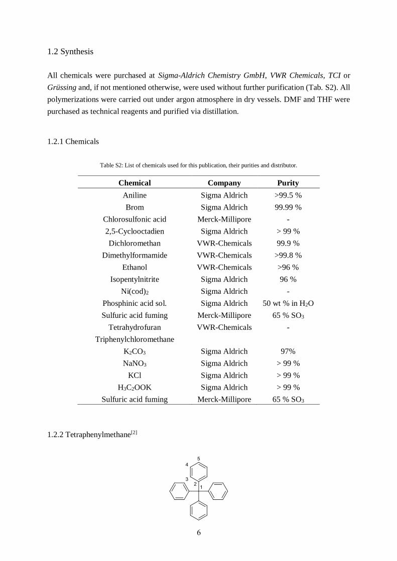
1.2.2 Tetraphenylmethane[2]

7

15 g of trityl chloride (0.054 mol, 1 eq.) and 14.05 ml aniline (0.154 mol, 2.9 eq.) were heated

up to 180 °C in a round flask with magnetic stirrer and condenser, until the reaction mixture

turned into a violet solid. The heating process was extended for 10 more minutes. The solid was

cooled down, crushed and resuspensed in 75 ml MeOH and 75 ml 2 M HCl. The Suspension

was refluxed for 30 min., filtered and washed with water. After resuspending in ethanol the

reaction mixture was cooled down to -30 °C and 15.75 ml sulfuric acid and 9.44 g of

isopentylnitrite (0.081 mol, 1.5 eq.) were added under vigorous stirring. After stirring for 1 h at

-10 °C, 26.9 ml of phosphinic acid (0.609 mol, 11 eq.) were added slowly and the reaction

mixture was refluxed for 1.5 h. After cooling down, the solid was filtered, washed with DMF,

H2O and Ethanol and subsequently dried in vacuo to get a light brown powder. Further

purification was not necessary but could be done by recrystallization in THF/methanol (1:1).

Yield: 16.1 g (0.05 mol, 93 %). 1H-NMR (500 MHz, DMSO-D6): δ [ppm] = 7.30 (t, 1H, H-4),

7.21 (t, 1H, H-5), 7.15 (d, 1H, H-3) (Fig. S3). 13C-NMR (500 MHz, DMSO-D6): δ [ppm] =

146.88 (C-2), 130.94 (C-3), 128.19 (C-4), 126.44 (C-5) (Fig. S4). EA [%]: C [91.25], H [6.54],

N [0.18]; Calc.: C [93.71], H [6.29], N [0.00]. MS [M/z] = 243, 320, 165. IR (ATR): ν [cm-1] =

1590, 1490, 1181, 1072, 1034, 767, 750, 696, 629, 491 (Fig. S7).

1.2.3 Tetrakis(4-bromophenyl)methane[3]

In a three necked vessel with magnetic stirrer, thermometer and condenser 10 g

tetraphenylmethane (31.2 mmol, 1 eq.) were cooled in an ice bath. Now 99.75 g Br2 (624 mmol,

20 eq.) were added dropwise. After cooling towards -78 °C, 140 ethanol (4.5 ml/mmol) were

applied and the mixture was allowed to reach room temperature overnight. Now

sodiumdisulfide solution was added until the end of precipitation. The resulting solid was

filtered, washed with H2O and dried in an oven at 110 °C. Further purification was carried out

performing recrystallization in a chloroform/ethanol mixture (1:1) to get a light brown solid.

Yield: 12.9 g (20.28 mmol, 65 %). 1H-NMR (500 MHz, DMSO-D6): δ [ppm] = 7.53 (d, 2H,

H-4), 7.06 (d, 2H, H-3) (Fig. S5). 13C-NMR (500 MHz, DMSO-D6): δ [ppm] = 63.66 (C-1),

120.40 (C-5), 131.55 (C-3), 132.86 (C-4), 145.06 (C-2) (Fig. S6). EA [%]: C [46.09], H [2.13];

Calc.: C [47.21], H [2.54]. MS [M/z] = 279, 239, 636, 319, 555, 198. IR (ATR): ν [cm-1] =

1569, 1486, 1393, 1181, 1072, 1005, 951, 908, 808, 750, 528, 507 (Fig. S7).

8

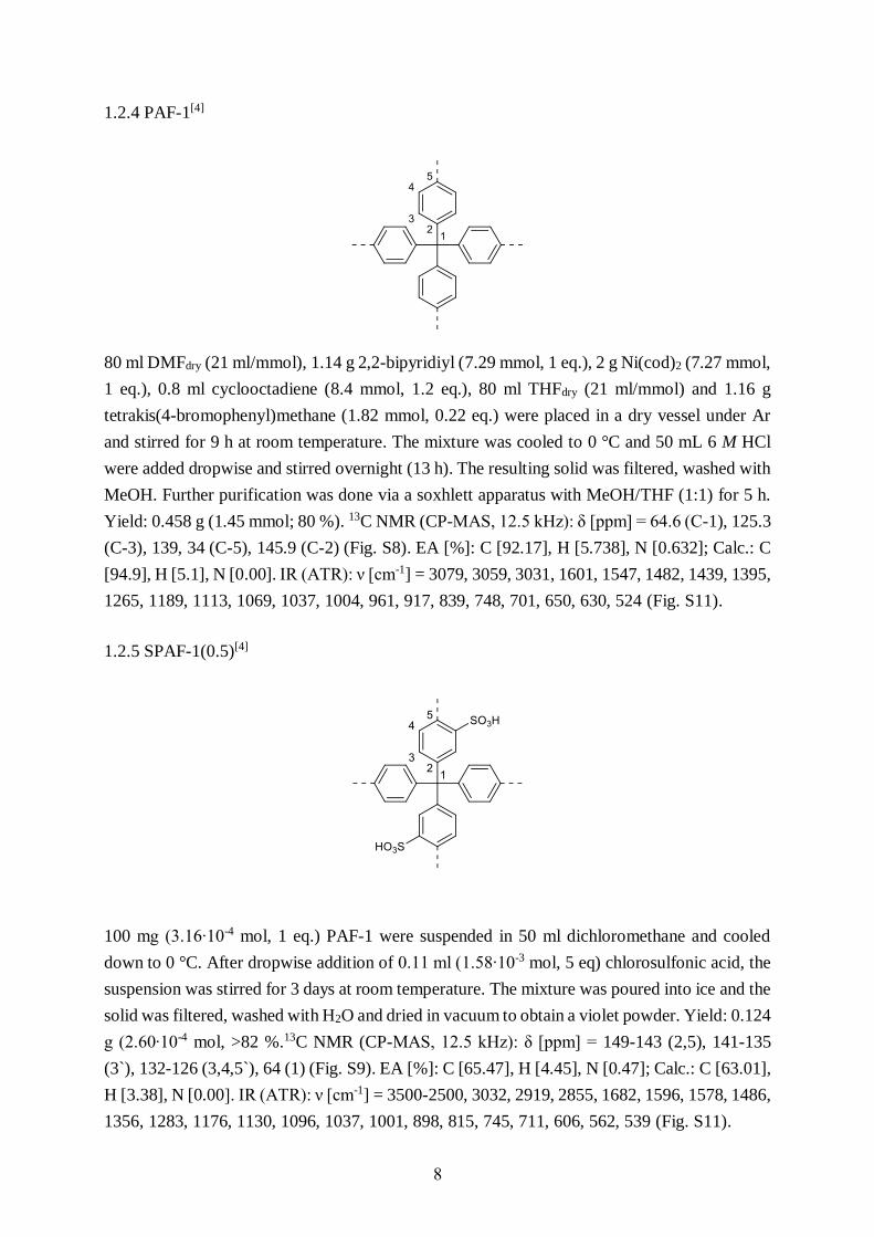
1.2.4 PAF-1[4]

80 ml DMFdry (21 ml/mmol), 1.14 g 2,2-bipyridiyl (7.29 mmol, 1 eq.), 2 g Ni(cod)2 (7.27 mmol,

1 eq.), 0.8 ml cyclooctadiene (8.4 mmol, 1.2 eq.), 80 ml THFdry (21 ml/mmol) and 1.16 g

tetrakis(4-bromophenyl)methane (1.82 mmol, 0.22 eq.) were placed in a dry vessel under Ar

and stirred for 9 h at room temperature. The mixture was cooled to 0 °C and 50 mL 6 M HCl

were added dropwise and stirred overnight (13 h). The resulting solid was filtered, washed with

MeOH. Further purification was done via a soxhlett apparatus with MeOH/THF (1:1) for 5 h.

Yield: 0.458 g (1.45 mmol; 80 %). 13C NMR (CP-MAS, 12.5 kHz): δ [ppm] = 64.6 (C-1), 125.3

(C-3), 139, 34 (C-5), 145.9 (C-2) (Fig. S8). EA [%]: C [92.17], H [5.738], N [0.632]; Calc.: C

[94.9], H [5.1], N [0.00]. IR (ATR): ν [cm-1] = 3079, 3059, 3031, 1601, 1547, 1482, 1439, 1395,

1265, 1189, 1113, 1069, 1037, 1004, 961, 917, 839, 748, 701, 650, 630, 524 (Fig. S11).

1.2.5 SPAF-1(0.5)[4]

100 mg (3.16∙10-4 mol, 1 eq.) PAF-1 were suspended in 50 ml dichloromethane and cooled

down to 0 °C. After dropwise addition of 0.11 ml (1.58∙10-3 mol, 5 eq) chlorosulfonic acid, the

suspension was stirred for 3 days at room temperature. The mixture was poured into ice and the

solid was filtered, washed with H2O and dried in vacuum to obtain a violet powder. Yield: 0.124

g (2.60∙10-4 mol, >82 %.13C NMR (CP-MAS, 12.5 kHz): δ [ppm] = 149-143 (2,5), 141-135

(3`), 132-126 (3,4,5`), 64 (1) (Fig. S9). EA [%]: C [65.47], H [4.45], N [0.47]; Calc.: C [63.01],

H [3.38], N [0.00]. IR (ATR): ν [cm-1] = 3500-2500, 3032, 2919, 2855, 1682, 1596, 1578, 1486,

1356, 1283, 1176, 1130, 1096, 1037, 1001, 898, 815, 745, 711, 606, 562, 539 (Fig. S11).

9

1.2.6 SPAF-1(1.25)

100 mg (3.16∙10-4 mol, 1 eq.) of PAF-1 were activated at 150 °C in vacuum for 2 h. Now fuming

sulfuric acid (65 % SO3) was applied via gas phase for 10 minutes (Figure SNumber). The

resulting solid was dried in vacuum at 150 °C for 1 h to yield a deep purple powder. Yield: 235

mg (3.28∙10-4 mol, >99 %). 13C NMR (CP-MAS, 12.5 kHz): δ [ppm] = 65.8 (C-1), 123.5 (C-

6), 130, 3 (C-7), 147.8 (C-2/4) (Fig. S10). EA [%]: C [41.31], H [3.71], N [0.53]; Calc.: C

[41.90], H [2.25], N [0.00]. IR (ATR): ν [cm-1] = 3500-2500, 1687, 1589, 1489, 1468, 1468,

1354, 1291, 1266, 1169, 1127, 1090, 1039, 1001, 938, 888, 825, 750, 712, 556, 507, 457 (Fig.

S11).

Figure S1: Schematic presentation of the gas phase sulfonation concept.

10

2. Analytical Section

2.1 Linker analytics

2.1.1 Liquid NMR

2.1.1.1 1H Tetraphenylmethane

10 8 6 4 2 0

DMSO (H2O)

Acetone

1H / ppm

Tetraphenylmethane

8.0 -6.5 ppm

DMSO

Figure S2: 1H liquid NMR spectra of Tetraphenylmethane.

2.1.1.2 13C Tetraphenylmethane

150 140 130 120 110 100

3

4

5

13

C / ppm

Tetraphenylmethane

2

Figure S3: 13C liquid NMR spectra of Tetraphenylmethane.

11

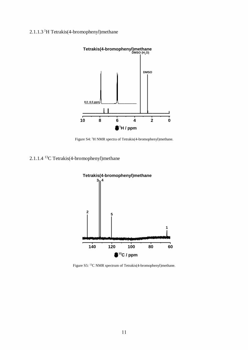
2.1.1.3 1H Tetrakis(4-bromophenyl)methane

10 8 6 4 2 0

8.0 -6.5 ppm

1H / ppm

Tetrakis(4-bromophenyl)methane

DMSO

DMSO (H2O)

Figure S4: 1H NMR spectra of Tetrakis(4-bromophenyl)methane.

2.1.1.4 13C Tetrakis(4-bromophenyl)methane

140 120 100 80 60

13

C / ppm


2

3 4

5

1

Figure S5: 13C NMR spectrum of Tetrakis(4-bromophenyl)methane.

12

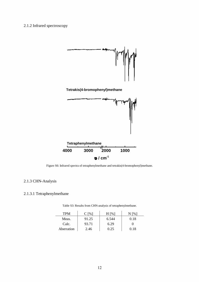
2.1.2 Infrared spectroscopy

4000 3000 2000 1000

/ cm-1

Tetraphenylmethane


Figure S6: Infrared spectra of tetraphenylmethane and tetrakis(4-bromophenyl)methane.

2.1.3 CHN-Analysis

2.1.3.1 Tetraphenylmethane

Table S3: Results from CHN-analysis of tetraphenylmethane.

TPM C [%] H [%] N [%]

Meas. 91.25 6.544 0.18

Calc. 93.71 6.29 0

Aberration 2.46 0.25 0.18

13

2.1.3.2 Tetrakis(4-bromophenyl)methane

Table S4: Results from CHN-analysis of tetrakis(4-bromophenyl)methane.

TBPM C H N

Meas. 46.09 2 0.08

Calc. 47.21 2.54 0

Aberration 1.12 0.41 0.08

2.2 Polymer analytics

2.2.1 Solid state NMR

2.2.1.1 13C_PAF-1

250 200 150 100 50 0

13

C / ppm

PAF-1

1

25

3

4

Figure S7: 13C CP MAS NMR spectrum of PAF-1.

Calculation of the crosslinking degree for PAF-1

The resonances of a quantitative MAS single pulse 13C spectrum (Figure S8) were deconvoluted

using a pseudo-Voigt lineshape with a 1:1 ratio for the Gaussian and Lorentzian components.

For 100 % crosslinking the intensity of C-5 (I(C-5)) should equal that of C2 (I(C-2)). Based on

the reaction mechanism of the used Yamamoto coupling, in case of an incomplete turnover we

expect either C-Br moieties (if no reaction occurred) or C-H moieties (if no CC coupling

occurred). Both signals are predicted to have 13C chemical shifts around 125 ppm (C-H) and

122 ppm (C-Br). Both resonances are thus superimposed with the signal for C4 and no

additional signals are expected. As a consequence, while I(C-5) reduces, I(C-4) is increased. At

the same time, I(C-2) should remain unaffected. Thus the intensity ratio I(C-5):(I(C-2)

estimated to 0.76(10) is a measure for the degree of crosslinking within the network.

14

200 180 160 140 120 100 80 60 40 20 0

PAF-1_13

C-MAS_12.5 kHz

13

C / ppm

2 5

34

1

Figure S8: 13C MAS onepulse NMR spectrum of PAF-1 for quantitative analysis.

Table 5: Fit parameter derived from the Gauss/Lorentz model based deconvolution of the 13C MAS onepuls spectrum of PAF-1 with an overlap of 95.17 %.

Sites 2 5 3 4 1

δ(iso) / ppm 146.19 139.8 130.9 125.7 64.5

LB / Hz 253.74 203.6 197.8 265.8 124.0

xG/(1-x)L 0.5 0.5 0.5 0.5 0.5

Integral 4.9 3.7 7.2 9.6 1

15

2.2.1.2 13C_SPAF-10.5

250 200 150 100 50 0

13

C / ppm

SPAF-1(0.5)

1

2,5

3,3`,4,4`,5`

Figure S9: 13C spectrum of SPAF-1(0.5).

2.2.1.3 13C_SPAF-1(1.25)

250 200 150 100 50 0

13

C / ppm

SPAF-1(1.25)

2,5`

3,6

3`

4

1

Figure S10: 13C spectrum of SPAF-1(1.25).

16

2.2.2 Infrared spectroscopy

4000 3000 2000 1000

/ cm-1

PAF-1

ring C-H str. vib.

OH-str.

OH-str.

Aryl-SO3H

SPAF-1(1.25)

OH-str.

OH-str.

SPAF-1(0.5)

Aryl-SO3H

Figure S11: Infrared spectra of PAF-1, SPAF-1(0.5) and SPAF-1(1.25).

2.2.3 CHN-Analysis

2.2.3.1 PAF-1 Table S6: Results from CHN-analysis of PAF-1.

Polymer C / % H / % N / %

PAF-1calc. 94.90 5.10 0.00

PAF-1meas. 92.17 5.74 0.63

Deviation 2.73 0.64 0.63

17

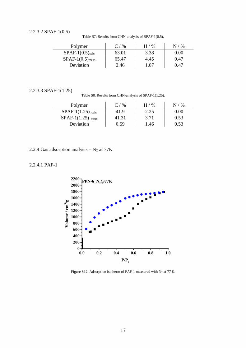
2.2.3.2 SPAF-1(0.5)

Table S7: Results from CHN-analysis of SPAF-1(0.5).


SPAF-1(0.5)calc 63.01 3.38 0.00

SPAF-1(0.5)meas 65.47 4.45 0.47

Deviation 2.46 1.07 0.47

2.2.3.3 SPAF-1(1.25) Table S8: Results from CHN-analysis of SPAF-1(1.25).


SPAF-1(1.25)_calc 41.9 2.25 0.00

SPAF-1(1.25)_meas 41.31 3.71 0.53

Deviation 0.59 1.46 0.53

2.2.4 Gas adsorption analysis – N2 at 77K

2.2.4.1 PAF-1

0.0 0.2 0.4 0.6 0.8 1.00

200

400

600

800

1000

1200

1400

1600

1800

2000

2200PPN-6_N

2@77K

Vo

lum

e /

cm3/g

P/P0

Figure S12: Adsorption isotherm of PAF-1 measured with N2 at 77 K.

18

0 2 4 6 8 10 12 14 16 18 20 22 240

1

2

3PPN-6_N

2@77K

Cu

mu

lati

ve

Po

re V

olu

me

/ c

m3g

-1

Porediameter / nm

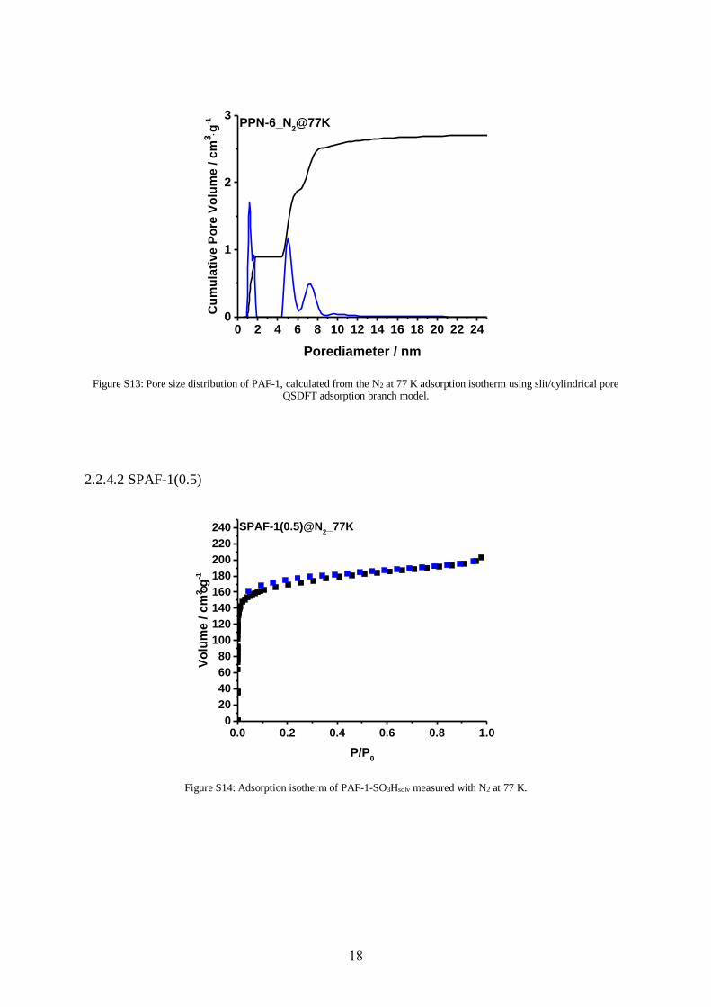
Figure S13: Pore size distribution of PAF-1, calculated from the N2 at 77 K adsorption isotherm using slit/cylindrical pore QSDFT adsorption branch model.

2.2.4.2 SPAF-1(0.5)

0.0 0.2 0.4 0.6 0.8 1.00

20

40

60

80

100

120

140

160

180

200

220

240 SPAF-1(0.5)@N2_77K

Vo

lum

e / c

m3g

-1

P/P0

Figure S14: Adsorption isotherm of PAF-1-SO3Hsolv measured with N2 at 77 K.

19

0 2 4 6 8 10 12 14 16 18 20 22 240.0

0.1

0.2

0.3

0.4SPAF-1(0.5)_N

2@77K

Porediameter / nm

Cu

mu

lati

ve P

ore

Vo

lum

e [

cm

3g

-1]

0.0

0.2

0.4

0.6

0.8

1.0

D(V

) /

cm

3n

m-1g

-1

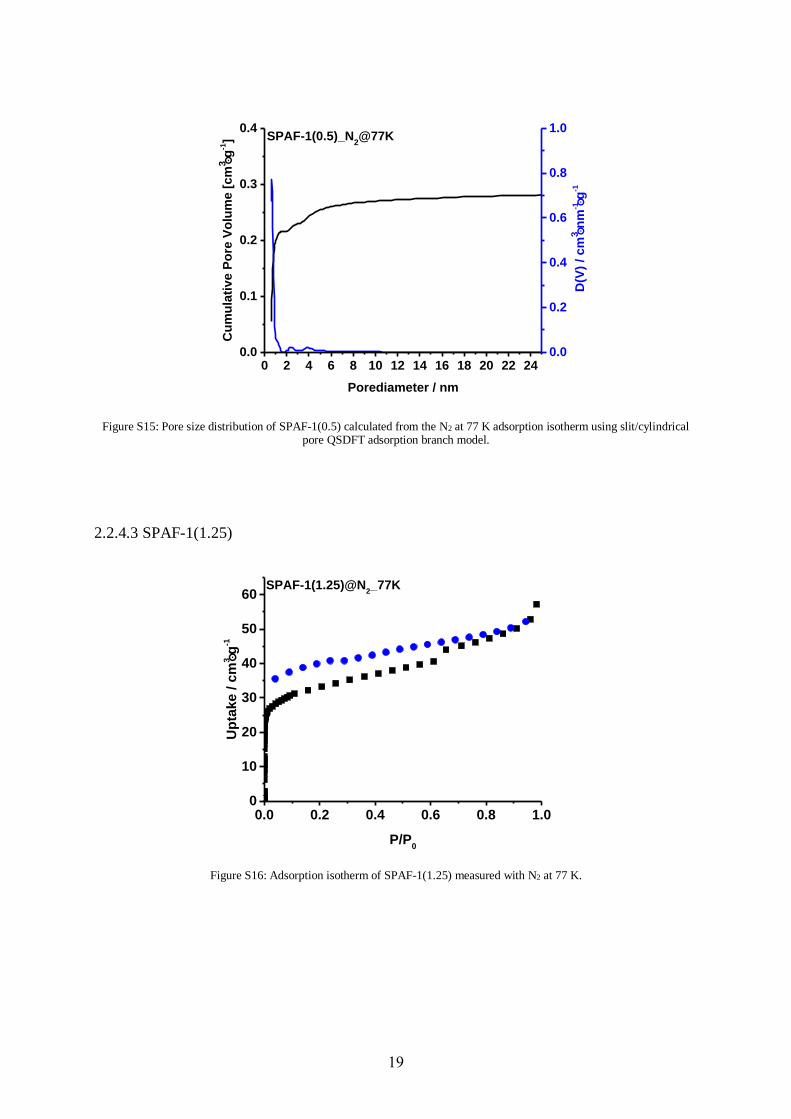
Figure S15: Pore size distribution of SPAF-1(0.5) calculated from the N2 at 77 K adsorption isotherm using slit/cylindrical pore QSDFT adsorption branch model.

2.2.4.3 SPAF-1(1.25)

0.0 0.2 0.4 0.6 0.8 1.00

10

20

30

40

50

60SPAF-1(1.25)@N

2_77K

Up

take

/ c

m3g

-1

P/P0

Figure S16: Adsorption isotherm of SPAF-1(1.25) measured with N2 at 77 K.

20

0 2 4 6 8 10 12 14 16 18 20 22 240.00

0.01

0.02

0.03

0.04

0.05

0.06

0.07

0.08SPAF-1(1.25)_N

2@77K_slit/cylindr.pores, QSDFT ads. branch

Porediameter / nm

Cu

mu

lati

ve P

ore

Vo

lum

e [

cm

3g

-1]

0.00

0.05

0.10

0.15

0.20

D(V

) /

cm

3n

m-1g

-1

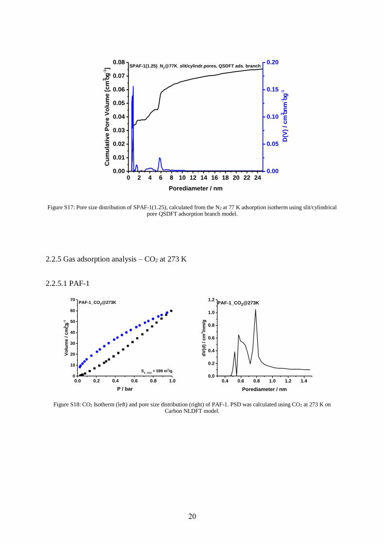
Figure S17: Pore size distribution of SPAF-1(1.25), calculated from the N2 at 77 K adsorption isotherm using slit/cylindrical pore QSDFT adsorption branch model.

2.2.5 Gas adsorption analysis – CO2 at 273 K

2.2.5.1 PAF-1

0.0 0.2 0.4 0.6 0.8 1.00

10

20

30

40

50

60

70PAF-1_CO2@273K

Vo

lum

e /

cm

3g

-1

P / bar

SA_CO2

= 599 m2/g

0.4 0.6 0.8 1.0 1.2 1.40.0

0.2

0.4

0.6

0.8

1.0

1.2

dV

(d)

/ c

m3/n

m/g

Porediameter / nm

PAF-1_CO2@273K

Figure S18: CO2 Isotherm (left) and pore size distribution (right) of PAF-1. PSD was calculated using CO2 at 273 K on Carbon NLDFT model.

21

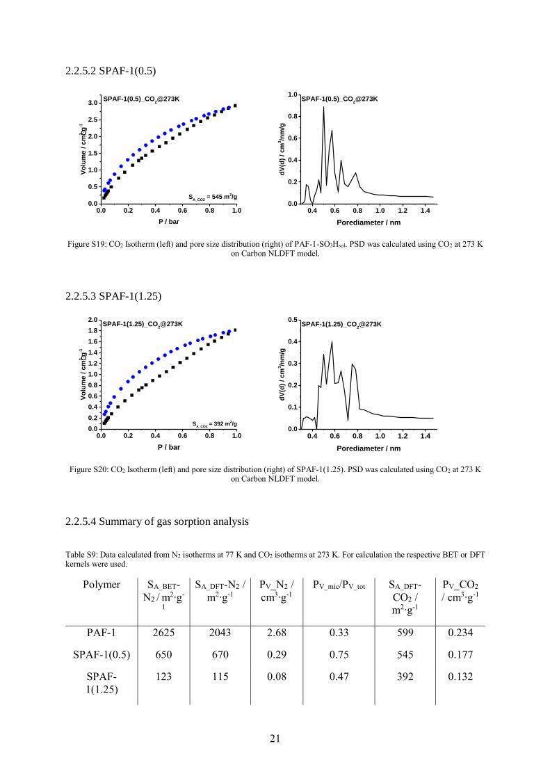
2.2.5.2 SPAF-1(0.5)

0.0 0.2 0.4 0.6 0.8 1.00.0

0.5

1.0

1.5

2.0

2.5

3.0SPAF-1(0.5)_CO

2@273K

Vo

lum

e / c

m3g

-1

P / bar

SA_CO2

= 545 m2/g

0.4 0.6 0.8 1.0 1.2 1.40.0

0.2

0.4

0.6

0.8

1.0

dV

(d)

/ cm

3/n

m/g

Porediameter / nm

SPAF-1(0.5)_CO2@273K

Figure S19: CO2 Isotherm (left) and pore size distribution (right) of PAF-1-SO3Hsol. PSD was calculated using CO2 at 273 K on Carbon NLDFT model.

2.2.5.3 SPAF-1(1.25)

0.0 0.2 0.4 0.6 0.8 1.00.0

0.2

0.4

0.6

0.8

1.0

1.2

1.4

1.6

1.8

2.0SPAF-1(1.25)_CO

2@273K

Vo

lum

e / c

m3g

-1

P / bar

SA_CO2

= 392 m2/g

0.4 0.6 0.8 1.0 1.2 1.40.0

0.1

0.2

0.3

0.4

0.5

dV

(d)

/ cm

3/n

m/g

Porediameter / nm

SPAF-1(1.25)_CO2@273K

Figure S20: CO2 Isotherm (left) and pore size distribution (right) of SPAF-1(1.25). PSD was calculated using CO2 at 273 K on Carbon NLDFT model.

2.2.5.4 Summary of gas sorption analysis

Table S9: Data calculated from N2 isotherms at 77 K and CO2 isotherms at 273 K. For calculation the respective BET or DFT kernels were used.

Polymer SA_BET-

N2 / m2‧g-

1

SA_DFT-N2 /

m2‧g-1

PV_N2 /

cm3‧g-1

PV_mic/PV_tot SA_DFT-

CO2 /

m2‧g-1

PV_CO2

/ cm3‧g-1

PAF-1 2625 2043 2.68 0.33 599 0.234

SPAF-1(0.5) 650 670 0.29 0.75 545 0.177

SPAF-

1(1.25)

123 115 0.08 0.47 392 0.132

22

2.2.6 TGA analysis

2.2.6.1 Stability

0 200 400 600 800 10000

20

40

60

80

100

We

igh

t / %

T / °C

PAF-1

SPAF-1(0.5)

SPAF-1(1.25)

Figure S21: Thermogravimetric data from PAF-1, SPAF-1(1.25) and SPAF-1(0.5), respectively. All Curves where measured under air with a 10 °C / min temperature ramp.

2.2.6.2 Water Uptake

Table S10: Water uptake versus theoretical pore volume for SPAF-1(0.5) and SPAF-1(1.25).

Polymer UptakeH2O@100%rH PV_theoretical

N2 Uptk.H2O/PV_theo.

SPAF-1(0.5) 0.65 cm3∙g-1 0.47 cm3∙g-1 1.38

SPAF-1(1.25) 1.68 cm3∙g-1 0.21 cm3∙g-1 8

23

2.2.7 UV-Vis spectroscopy

200 300 400 500 600 700 8000.0

0.2

0.4

0.6

0.8

1.0

ab

so

rban

ce

/ nm

PAF-1 -hydrated

SPAF-1(1.25) -hydrated

SPAF-1(0.5) -hydrated

Figure S22: UV-VIS spectra of PAF-1, SPAF-1(1.25) and SPAF-1(0.5), respectively. Full lines show the absorbance of the polymers in the dry state, dashed lines stand for fully hydrated state.

2.2.8 Powder X-ray diffraction

5 10 15 20 25 30

2 / °

PAF-1

SPAF-1(1.25)

SPAF-1(0.5)

Figure S23: PXRDs of PAF-1, SPAF-1(1.25) and SPAF-1(0.5).

24

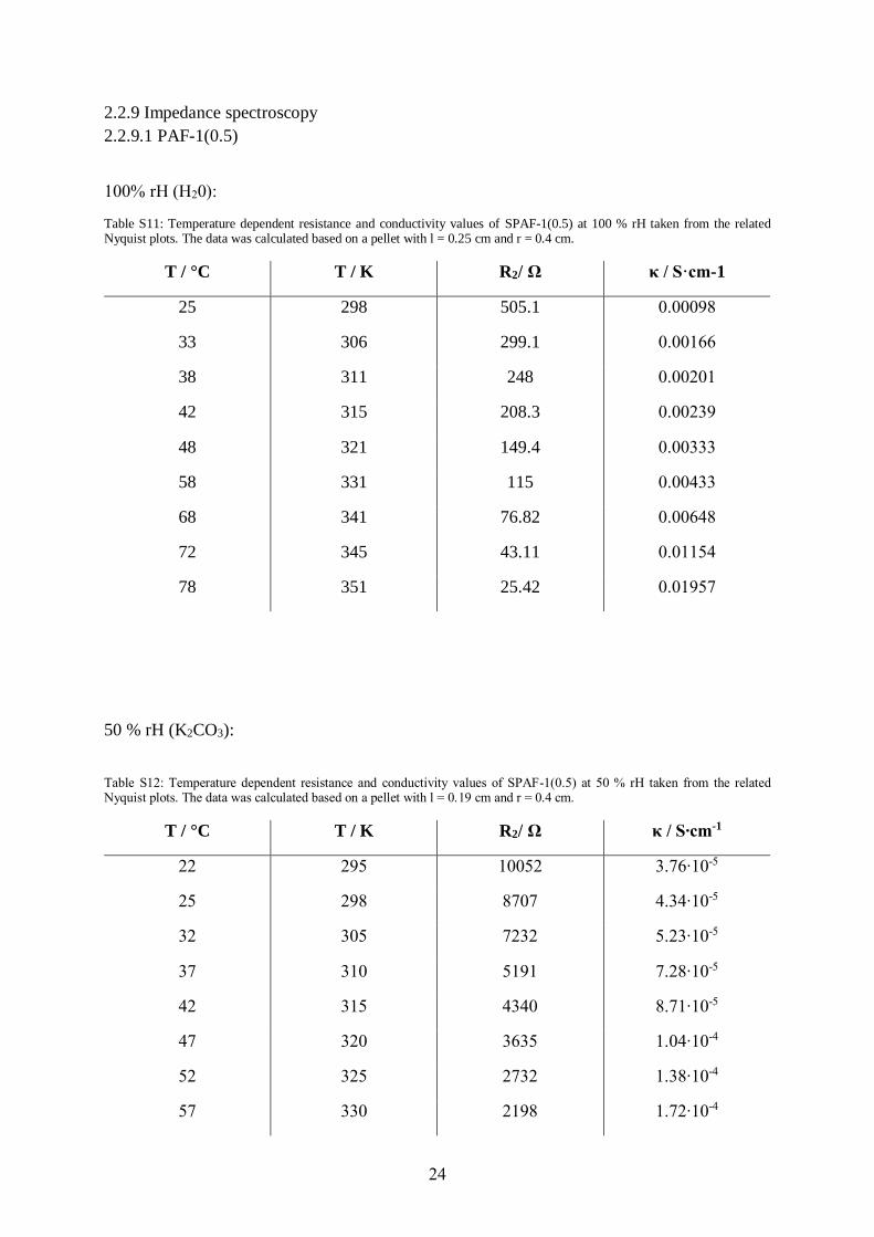
2.2.9 Impedance spectroscopy

2.2.9.1 PAF-1(0.5)

100% rH (H20):

Table S11: Temperature dependent resistance and conductivity values of SPAF-1(0.5) at 100 % rH taken from the related Nyquist plots. The data was calculated based on a pellet with l = 0.25 cm and r = 0.4 cm.

T / °C T / K R2/ Ω κ / S·cm-1

25 298 505.1 0.00098

33 306 299.1 0.00166

38 311 248 0.00201

42 315 208.3 0.00239

48 321 149.4 0.00333

58 331 115 0.00433

68 341 76.82 0.00648

72 345 43.11 0.01154

78 351 25.42 0.01957

50 % rH (K2CO3):


T / °C T / K R2/ Ω κ / S∙cm-1

22 295 10052 3.76∙10-5

25 298 8707 4.34∙10-5

32 305 7232 5.23∙10-5

37 310 5191 7.28∙10-5

42 315 4340 8.71∙10-5

47 320 3635 1.04∙10-4

52 325 2732 1.38∙10-4

57 330 2198 1.72∙10-4

25

60 333 1850 2.04∙10-4

68 341 1513 2.49∙10-4

71 344 1341 2.82∙10-4

77 350 1214 3.11∙10-4

30 % rH (H3C2OOK):


T / °C T / K R2/ Ω κ / S∙cm-1

22 295 138830 2.87∙10-6

25 298 110690 3.59∙10-6

30 303 77582 5.13∙10-6

35 308 58635 6.79∙10-6

40 313 46654 8.53∙10-6

45 318 35636 1.12∙10-5

50 323 29521 1.35∙10-5

57 330 24057 1.65∙10-5

63 336 18073 2.20∙10-5

65 338 14929 2.67∙10-5

70 343 11757 3.38∙10-5

75 348 8648 4.60∙10-5

80 353 7375 5.40∙10-5

26

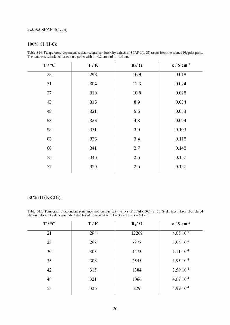
2.2.9.2 SPAF-1(1.25)

100% rH (H20):

Table S14: Temperature dependent resistance and conductivity values of SPAF-1(1.25) taken from the related Nyquist plots. The data was calculated based on a pellet with l = 0.2 cm and r = 0.4 cm.

T / °C T / K R2/ Ω κ / S∙cm-1

25 298 16.9 0.018

31 304 12.3 0.024

37 310 10.8 0.028

43 316 8.9 0.034

48 321 5.6 0.053

53 326 4.3 0.094

58 331 3.9 0.103

63 336 3.4 0.118

68 341 2.7 0.148

73 346 2.5 0.157

77 350 2.5 0.157

50 % rH (K2CO3):


T / °C T / K R2/ Ω κ / S∙cm-1

21 294 12269 4.05∙10-5

25 298 8378 5.94∙10-5

30 303 4473 1.11∙10-4

35 308 2545 1.95∙10-4

42 315 1384 3.59∙10-4

48 321 1066 4.67∙10-4

53 326 829 5.99∙10-4

27

58 331 654 7.60∙10-4

62 335 564 8.82∙10-4

66 339 590 8.43∙10-4

72 345 450 0.00111

77 350 389 0.00128

80 353 386 0.00129

30 % rH (H3C2OOK):


T / °C T / K R2/ Ω κ / S∙cm-1

22 295 84342 4.24∙10-6

25 298 73798 4.85∙10-6

30 303 56344 6.35∙10-6

35 308 40898 8.77∙10-6

40 313 29112 1.23∙10-5

45 318 20231 1.77∙10-5

50 323 13869 2.58∙10-5

55 328 11939 2.99∙10-5

62 335 8364 4.28∙10-5

66 339 7245 4.94∙10-5

70 343 5509 6.49∙10-5

75 348 4221 8.48∙10-5

80 353 3366 1.06∙10-4

28

2.2.10 Differential scanning calorimetry

200 250 300 350 400

-25

-20

-15

-10

-5

0

5

10

15

Heat

flo

w / m

W

T / K

SPAF-1(1.25)@30 % rH

Endo

Exo

200 250 300 350 400

-25

-20

-15

-10

-5

0

5

10

15

Exo

Heat

flo

w / m

W

T / K

SPAF-1(1.25)@100 % rH

Endo

Figure S24: DSC curves for SPAF-1(1.25) hydrated at 30 % (top) and 100 % rH (bottom).

For SPAF-1(1.25) saturated for 100 %rH (Figure S24 bottom) an endothermic melting peak at

around -25 °C with an area equivalent to 0.35 J was observed. With a melting enthalpy (ΔHm)

for water of 333.5 J/g, this corresponds to 0.06 mmol water. In contrast, TG measurements

revealed a total amount of 0.23 mmol water to be adsorbed within the network. Thus, only 25 %

of the incorporated water is stored in mesopores, while 85 % is located in micropores.

29

2.2.11 Energy dispersive X-ray spectroscopy

Figure S25: REM image of Na-SPAF-1(1.25).

30

Figure S26: EDX spectra of Na-SPAF-1(1.25) without coloration, blue colorized sulfur distribution, violet colorized sodium distribution.

2.2.12 Atomic force microscopy

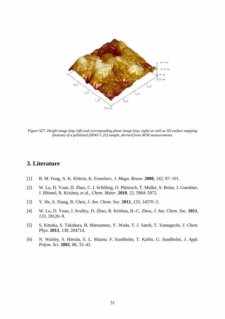
31

Figure S27: Height image (top, left) and corresponding phase image (top, right) as well as 3D surface mapping

(bottom) of a pelletized (SPAF-1.25) sample, derived from AFM measurements.

3. Literature

[1] B. M. Fung, A. K. Khitrin, K. Ermolaev, J. Magn. Reson. 2000, 142, 97–101.

[2] W. Lu, D. Yuan, D. Zhao, C. I. Schilling, O. Plietzsch, T. Muller, S. Bräse, J. Guenther,

J. Blümel, R. Krishna, et al., Chem. Mater. 2010, 22, 5964–5972.

[3] Y. He, S. Xiang, B. Chen, J. Am. Chem. Soc. 2011, 133, 14570–3.

[4] W. Lu, D. Yuan, J. Sculley, D. Zhao, R. Krishna, H.-C. Zhou, J. Am. Chem. Soc. 2011,

133, 18126–9.

[5] S. Kittaka, S. Takahara, H. Matsumoto, Y. Wada, T. J. Satoh, T. Yamaguchi, J. Chem.

Phys. 2013, 138, 204714.

[6] N. Walsby, S. Hietala, S. L. Maunu, F. Sundholm, T. Kallio, G. Sundholm, J. Appl.

Polym. Sci. 2002, 86, 33–42.

water mediated proton conduction in a sulfonated ... · water mediated proton conduction in a...

Documents