Water Availability and Global Land Use Change

By

Jing Liu, Farzad Taheripour, and Thomas W. Hertel

Authors’ Affiliation

Jing Liu is Ph.D. Student, Farzad Taheripour is Research Assistant Professor, and Thomas W.

Hertel is distinguished Professor in the Department of Agricultural Economics at Purdue

University.

Revision 1

June 2012

Department of Agricultural Economics

Purdue University

To be presented at:

15th Annual Conference on Global Economic Analysis

"New Challenges for Global Trade and Sustainable Development"

Geneva, Switzerland June 27-29, 2012

Water Availability and Global Land Use Change

Jing Liu, Farzad Taheripour, Thomas Hertel

Introduction

The dual stressors of surging water demand and climate-induced variable water supply signal that

global economy is entering an era of water scarcity. Under the scenario of average economic growth with

no efficiency gains, global water requirements by 2030 would grow from 4,500 billion m3 today to 6,900

billion m3, which is a full 40 percent above current accessible, reliable supply (Addams, et al. 2009). In

addition, water’s two fundamental functions, the role as an essential requirement for life and its use as an

economic input, are increasingly in conflict. If assume that water for agriculture is low-priority use and

water demand-supply gap is closed by cutting down irrigation, the impact of water deficit on agriculture

can be sizable given the fact that irrigated agriculture accounts for up to 70 percent of global water

withdraw (FAO, Agriculture, food and water 2003).

Globally, 20 percent of the cultivated land is irrigated and contributes over 40 percent of the food

supplies. On average, irrigated crop yield is 2.3 times higher than those from rainfed crop, globally (FAO,

Irrigation Management Transfer 2007). Shortage of irrigation water under the business-as-usual scenario

will slow down the expansion of irrigated agricultural and can even make it impossible. By implication,

more rainfed land is needed to meet the demand for the same amount of food since the productivity of

irrigated agriculture is generally higher than that of rainfed. The expansion of rainfed agriculture could

lead a higher rate of deforestation and cause more induced land use emissions. Nevertheless, the

feasibility of this solution is not universally guaranteed. The region where physical expansion is limited

has to import more from or export less to global market to satisfy domestic demand. Water deficit thus

speaks to global land use change and pattern of agricultural trade.

Literature review

Most of the existing research on global land use change commingled irrigated and rainfed

production due to the lack of necessary data at international dimension. By doing so, the productivity of

new lands is inflated. Land conversion and its impact tend to be understated. For example, Pfister et al.

compare the trade-off between land and water consumption under four strategies to meet future world

food demand. They find that land expansion on pastures is pretty low due to high-yield production

(Pfister, et al. 2011)., The yield they considered, however, is averaged over two types of production,

Several studies emerged as the earliest attempts to distinguish crop production between irrigation

conditions. IMPACT-WATER model has been used to explore the impact of water availability on food

supply and demand (Rosegrant, Cai and Cline 2002) and virtual water trade (de Fraiture, et al. 2004). As a

partial equilibrium model, it examines effects of policy action in the particular market which is directly

affected, but ignores its effect on any other. A global CGE model GTAP-W developed by Calzadilla et al.

discomposes land endowment used in crop industries into the contribution of water, irrigated land, and

rainfed land, based on the ratio of yields and output by irrigation condition provided by IMPACT. Using

this model, the authors investigate the potential global water savings and its economic implications by

improving irrigation efficiency (Calzadilla, Rehdanz and Tol 2011). A major shortcoming of GTAP-W is

that it is essentially built on value reallocation but does not consider physical change of land and water.

For example, agricultural land is fixed; increase in irrigated land causes decrease in non-irrigated land by

the same amount, and vice versa. Besides, land and water data serving the value split are uniform within

FPUs (Food Production Unit), which is less satisfactory when FPU is large.

A recent paper by Taheripour et al. (henceforth THL) moves further in this direction (Taheripour,

Hertel and Liu 2011). The paper investigated the role of irrigation in determining the global land

conversion in the wake of increased ethanol production. In this work, crop industries in GTAP v.6

database are broken into irrigated and rainfed categories based on Portmann et al. (2010). Furthermore,

the GTAP-BIO-AEZ model is modified and extended to handle production, consumption and trade of

irrigated and rainfed crops, and to trace the allocation of irrigated and rainfed cropland among all crop

activities at a global scale. In spite of its utility in the analysis that involves irrigated and rainfed

agriculture, it fails to detach water from irrigated land and thus is limited in its use for examining the role

of managed water in agriculture and land use change. The present research aims to address this deficiency

and explicitly introduce managed water into database and modeling framework.

Data and modeling

We begin with a grid-based dataset containing crop specific global harvested area and yield,

provided by Portmann et al. (Portmann, Siebert and Döll 2010). The original resolution (5 arc minute)

was reduced to 30 arc minute (i.e. half degree) in order to accommodate other existing data. We identify

country, AEZ and river basin associated with each grid cell in ArcGIS, and aggregate grid-based

information up to region-AEZ-Basin by crop. Altogether, we have 6 crops, 19 regions, 18 AEZs and a

maximum number of 20 basins per region in the base data (see Appendix for the basin names).

The result of above process, along with the region-AEZ indexed data developed in THL, is used

to determine the value added of land at region-AEZ-Basin level. To be specific, we break region-AEZ

value added of land into region-AEZ-Basin value added of land by multiplying the former with a

production share that depicts the contribution of each basin within a certain AEZ. Then we extend GTAP

regional input-out tables by considering water as a primary input of irrigated crop production functions.

Under the assumption that yield gap between irrigated and rainfed crops is totally attributed to

irrigation, we use values-based productivity difference and area at each river basin to determine the cost

share of water for irrigated crop productions. Utilizing another grid-based dataset developed by Siebert

and Döll (Siebert and Döll 2010) on water used for irrigation, we aggregate quantity of water used by

crop into basin-AEZ in each region. The procedure up to this point prepares us the quantity as well as

value added of land and water by region-AEZ-river basin.

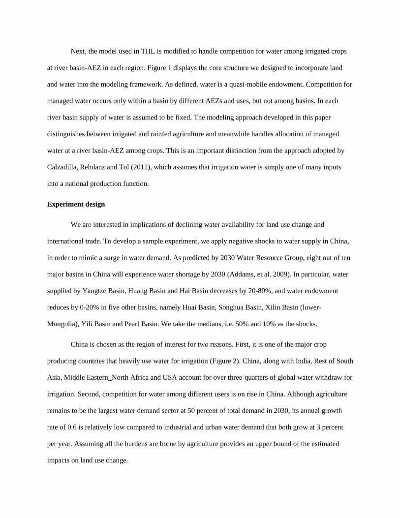
Next, the model used in THL is modified to handle competition for water among irrigated crops

at river basin-AEZ in each region. Figure 1 displays the core structure we designed to incorporate land

and water into the modeling framework. As defined, water is a quasi-mobile endowment. Competition for

managed water occurs only within a basin by different AEZs and uses, but not among basins. In each

river basin supply of water is assumed to be fixed. The modeling approach developed in this paper

distinguishes between irrigated and rainfed agriculture and meanwhile handles allocation of managed

water at a river basin-AEZ among crops. This is an important distinction from the approach adopted by

Calzadilla, Rehdanz and Tol (2011), which assumes that irrigation water is simply one of many inputs

into a national production function.

Experiment design

We are interested in implications of declining water availability for land use change and

international trade. To develop a sample experiment, we apply negative shocks to water supply in China,

in order to mimic a surge in water demand. As predicted by 2030 Water Resource Group, eight out of ten

major basins in China will experience water shortage by 2030 (Addams, et al. 2009). In particular, water

supplied by Yangtze Basin, Huang Basin and Hai Basin decreases by 20-80%, and water endowment

reduces by 0-20% in five other basins, namely Huai Basin, Songhua Basin, Xilin Basin (lower-

Mongolia), Yili Basin and Pearl Basin. We take the medians, i.e. 50% and 10% as the shocks.

China is chosen as the region of interest for two reasons. First, it is one of the major crop

producing countries that heavily use water for irrigation (Figure 2). China, along with India, Rest of South

Asia, Middle Eastern_North Africa and USA account for over three-quarters of global water withdraw for

irrigation. Second, competition for water among different users is on rise in China. Although agriculture

remains to be the largest water demand sector at 50 percent of total demand in 2030, its annual growth

rate of 0.6 is relatively low compared to industrial and urban water demand that both grow at 3 percent

per year. Assuming all the burdens are borne by agriculture provides an upper bound of the estimated

impacts on land use change.

Results

Impacts on output and price of crops and other commodities

In China, crop production highly relies on irrigation. 44.8% of the harvested area is irrigated and

44.2% of the total crop output comes from land with irrigation. In addition, the country contributes a

considerable share to the global irrigated crop production. For example, China produces almost 40% of

irrigated rice, 36% of irrigated wheat and 37% of irrigated coarse grains of the world. In consequence,

water shortage is expected to sharply reduce crop production in China and subsequently world food

supply. According to our results (Table 1), paddy rice will see the most dramatic reduction in output (9.3

million m.t.), followed by other agricultural produces (mainly fruit and vegetables, 5.2 million m.t.) and

wheat (3.2 million m.t.). This pattern of change is largely driven by two facts. First, the shocked basins

represent major agricultural zones in China. 92% of the country’s crop production is concentrated in these

basins. Second, cereal grains and other agricultural produces take the lion’s share of irrigation water

within the basins. Figure 3 provides a “zoom-in” on each affected crops. As anticipated, irrigated

production goes down, while rainfed production expands. Although output of rice sees the largest

reduction in total, irrigated fruit and vegetable turn out to be the most affected sector in absolute terms.

At the same time, output of most crops in non-China countries raises slightly because of the lower

endowment cost to produce the same amount of crops in these countries. The raise, however, can only

partially offset what is lost in China, especially for rice, wheat and coarse grains, the major cereal grains

that China accounts for over one third of the world irrigated production. Globally speaking, value based

output drops by 0.71% for rice and 0.21% for wheat due to limited water supply in China (Table 2).

Under the assumption that products are differentiated and price differs across regions, this set of result

mingles changes of both price and quantity. It may draw a different picture from what implied by quantity

alone. For example, using the tons measure, sugar production falls globally, but using the GTAP index it

rises.

Downscaled crop production provides less input for processed food and less feed for livestock

raising, leading to shrinking output in these industries as well. Prices go up as the supply of these

commodities goes down. Opposite to what is generally observed for agricultural and food sectors, energy

related and manufacturing industries thrive. Supply price of these commodities falls. The change is more

pronounced in China than in the other regions.

Impacts on international trade

Table 3 summarizes change in trade balance for selected countries and commodities. A negative

value indicates that the change in imports exceeds the change in exports. Table 4a and 4b present the

percentage changes of China’s food and agricultural products imports and exports with primary trade

partners. Not surprisingly, reduction in crop output suppresses China’s crop export to the world and, on

the other hand, causes the country to import more agricultural commodities to meet domestic demand for

food. Total trade gap in agriculture and food amounts to 1.9 billion US dollars, with more than half of it

attributable to crop trade deficit. The biggest trade deficits are observed in the trade of fruit, vegetables

and processed food, partly due to their high value compared to the other field crops. More importantly, it

has been a basic policy for food security in China that maintaining a high level of grain self-sufficiency

should not be compromised and all possible efforts will be made to ensure production of staple food. It’s

also worth noting that China tends to import more oilseeds and livestock from international market. Its

domestic oilseed production has been on a declining trend in recent years as a result of reduced acreage

devoted to oilseeds and little or no growth in average yields. For this reason, China’s dependence on

South America and US oilseeds is expected to increase. Rising consumption of meat, particularly of pork,

is considered as a major driver for the widening trade deficit in livestock products. China's meat imports

will continue to rise due to strong pork demand and competitive pricing on imports.

U.S. and EU, two key players in global agricultural market, will export more food (especially the

processed food) to China and rest of the world. Total trade balance of U.S. and EU, however, would get

worse due to the enlarged trade deficit in industrial goods. Other big economies such as Japan, Brazil and

Canada more or less tell the same story. China instead will expand its non-agricultural commodity export

(primarily manufacturing exports) in order to keep its current account in surplus. The simulation results

show a significant boost (3.1 billion USD) in the trade balance of manufacturing industries, followed by

increased net exports in energy intensive industries (0.34 billion USD), crude oil, and petroleum and coal

products sectors.

Land cover implications

Water scarcity can make irrigation physically impossible or so costly that producing irrigated

crops is no longer economically viable. Comparatively, rainfed crop production can be more profitable

and may crowd out the irrigated (if assume that climate change will not jeopardize rainfed agriculture).

To compensate for the lost irrigated production, more rainfed land is needed because output per hectare is

generally lower when crop growth relies solely on rainfall. Table 5 shows a production shift from the

irrigated to the rainfed land in China. When confronted with water scarcity, irrigation will be discontinued

for 7.5 million hectares of land. These parcels are turned into rainfed fields that are no longer able to

output the same amount of food due to lower productivity. To maintain current level of crop production,

this region needs an addition of 0.69 million hectares rainfed land, which is about 0.42% of the total

harvested area in China. The relatively small amount of additional land needed can be explained by

moderate yield gains when crops are irrigated in China. Among 6 major crops, irrigation matters most for

sugar crops. With irrigation, output per hectare can be 1.73 times higher than if with no irrigation. Yield

of irrigated rice is about 50% higher than that of the rainfed. For wheat, coarse grains, oil seeds and fruits

and vegetables, this number is even lower. Irrigation means only 20% productivity gains.

As China shrinks its food supply to the world, the gap needs to be filled by harvest from other

regions. This leads to 1.12 million hectares of new land to be cultivated globally for raising crops. The

most significant expansion occurs in Sub-Saharan Africa, Canada, EU, Brazil and US. The expansion is

mainly contributed by the enlargement of rainfed areas, which takes more than 85% of the total. This is

sensible given that irrigation involves high investment. Figure 4 depicts total crop cover (irrigated plus

rainfed) expansion of the world at river basin level. Apart from several major basins in China, Red River

and Lake Winnipeg basins in North America, Paraná basin in South America and Niger basin in Africa

will be the places where large crop land expansion is most likely to occur.

As for the composition of land conversion, over 60% of the new crop land in China comes at the

expense of pasture land (Table 6). Globally, this number is even higher, up to 73%. It suggests that most

regions will mainly convert grazing land to support crop production. A few exceptions are EU, Canada

and Japan, where over half of the converted land used to be forestland, indicating that these regions may

see more deforestation and exhibit higher emission factors.

Implications for water demand

Less water availability drives up water prices. Water becomes a more expensive input for

irrigated crop production in the related basins. In our model, production function is allowed to be different

across AEZs within a basin. The optimal level of water input is then determined at each AEZ depending

on how efficiently water can be used. In other words, water use will be suppressed in the AEZs that have

a higher cost share of water, and vice versa. Moreover, water for irrigation is competed by different crops

within each basin-AEZ. The crop that takes the lion’s share of irrigation will suffer most.

Table 7 and 8 paint a more nuanced picture of the changes described above by focusing on

Yangtze basin, China. It is one of the basins that will see the greatest water supply shrinkage in the future.

Besides, it irrigates the most important agricultural zone in China. Interestingly, although it is well known

that rice production consumes lots of water, it turns out to be very efficient in water usage, probably

because of better farming practice and knowledge, as well as the endogenous location choice. In contrast,

water is a relatively costly input to produce sugar crops. As expected, water is released from the

production of sugar crops to support cultivation of other crops. If look across AEZs, production tends to

rise in zones that pay less for the water bills, and vice versa. Take coarse grain as an example. Production

is attracted to AEZ 11, where water inputs accounts for a smaller cost compared to land rent, from the

other AEZs where production is less water-efficient.

Implications for regional welfare

Table 9 shows the regional household Equivalent Variation, resulting from China water supply

shock. Large welfare reduction is observed in China. Likewise, households in EU, East Asia are worse

off. US will see a moderate utility gain. (Needs more work to show decomposition of EV.)

Conclusion

We present an improved general equilibrium model and the associated datasets that can be used

to analyze water-related economic issues at global scale. This new framework tells apart two types of

crop production activities, irrigated and rainfed that are featured by different productivity, cost structure

and level of difficulty to expand. The distinction enables refined analysis of economic consequences

caused by policy and environmental factors, which otherwise compounds the effects of the two.

Furthermore, the present approach highlights the explicit inclusion of water as a production input.

Quantity as well as value of water can be allocated to achieve economic equilibrium. These

modifications significantly increase the flexibility of existing CGE modeling, especially when the

application involves land and water use.

Utilizing the updated model and dataset, we experiment on water deficit in China and analyze its

effects on global land use change and international trade. We assumed that widening water gap in China

would cut back its irrigated crop production. Total crop output falls as non-irrigated field is not good

enough to make up for the lost productivity. The country’s balance of agricultural trade worsens. To even

out the imbalance, a larger trade surplus in non-agricultural goods is needed. Crop production continues

to compete for land from forestry and livestock sectors. Over one third of the converted crop land comes

from deforestation.

The numerical results suggest that a localized shock to water availability affects global land cover.

A portion of irrigated production, which is hard to expand in China, shifts towards other regions,

primarily U.S. and Europe. Expansion of rainfed crop production appears to be more notable and happens

almost everywhere but particularly in U.S., EU, Canada, Brazil and Sub-Saharan Africa. The new crop

land mainly comes from grazing land and may put pressure on the livestock industry to grow.

Environmental concerns might rise due to deforestation and grassland conversion occurred in the

areas that have high emission factors (e.g. Latin America). In conclusion, water shortage in China may

significantly reduce the country’s crop output and its food supply to the world. International trade buffers

the shock of regional water supply variability, but the effects of shrinking irrigated areas in China spill

over to other regions, causing worldwide crop land expansion.

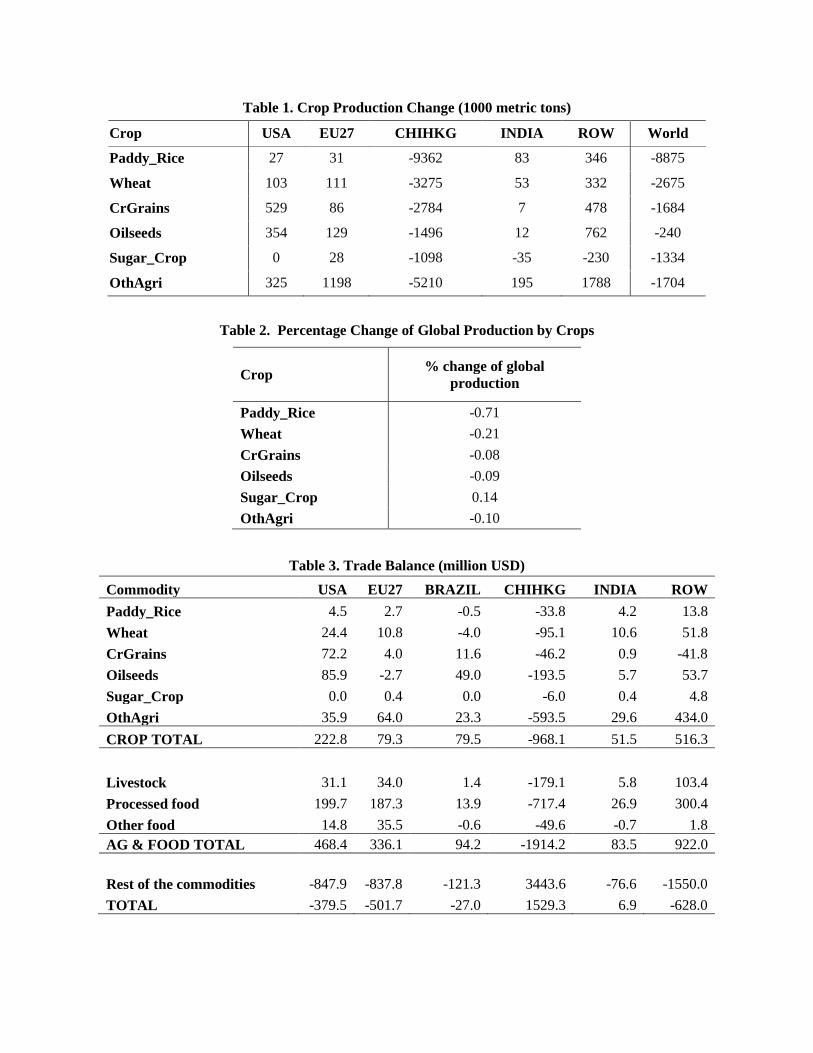
Table 1. Crop Production Change (1000 metric tons)

Crop USA EU27 CHIHKG INDIA ROW World

Paddy_Rice 27 31 -9362 83 346 -8875

Wheat 103 111 -3275 53 332 -2675

CrGrains 529 86 -2784 7 478 -1684

Oilseeds 354 129 -1496 12 762 -240

Sugar_Crop 0 28 -1098 -35 -230 -1334

OthAgri 325 1198 -5210 195 1788 -1704

Table 2. Percentage Change of Global Production by Crops

Crop % change of global

production

Paddy_Rice -0.71

Wheat -0.21

CrGrains -0.08

Oilseeds -0.09

Sugar_Crop 0.14

OthAgri -0.10

Table 3. Trade Balance (million USD)

Commodity USA EU27 BRAZIL CHIHKG INDIA ROW

Paddy_Rice 4.5 2.7 -0.5 -33.8 4.2 13.8

Wheat 24.4 10.8 -4.0 -95.1 10.6 51.8

CrGrains 72.2 4.0 11.6 -46.2 0.9 -41.8

Oilseeds 85.9 -2.7 49.0 -193.5 5.7 53.7

Sugar_Crop 0.0 0.4 0.0 -6.0 0.4 4.8

OthAgri 35.9 64.0 23.3 -593.5 29.6 434.0

CROP TOTAL 222.8 79.3 79.5 -968.1 51.5 516.3

Livestock 31.1 34.0 1.4 -179.1 5.8 103.4

Processed food 199.7 187.3 13.9 -717.4 26.9 300.4

Other food 14.8 35.5 -0.6 -49.6 -0.7 1.8

AG & FOOD TOTAL 468.4 336.1 94.2 -1914.2 83.5 922.0

Rest of the commodities -847.9 -837.8 -121.3 3443.6 -76.6 -1550.0

TOTAL -379.5 -501.7 -27.0 1529.3 6.9 -628.0

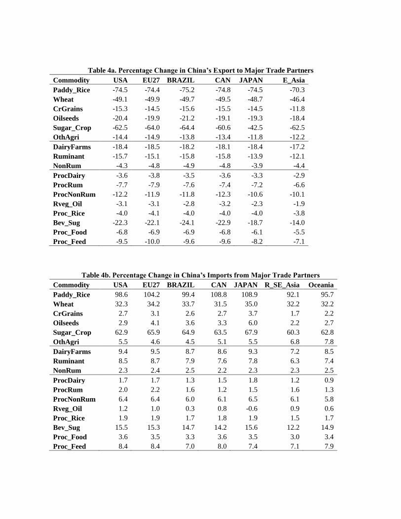
Table 4a. Percentage Change in China’s Export to Major Trade Partners

Commodity USA EU27 BRAZIL CAN JAPAN E_Asia

Paddy_Rice -74.5 -74.4 -75.2 -74.8 -74.5 -70.3

Wheat -49.1 -49.9 -49.7 -49.5 -48.7 -46.4

CrGrains -15.3 -14.5 -15.6 -15.5 -14.5 -11.8

Oilseeds -20.4 -19.9 -21.2 -19.1 -19.3 -18.4

Sugar_Crop -62.5 -64.0 -64.4 -60.6 -42.5 -62.5

OthAgri -14.4 -14.9 -13.8 -13.4 -11.8 -12.2

DairyFarms -18.4 -18.5 -18.2 -18.1 -18.4 -17.2

Ruminant -15.7 -15.1 -15.8 -15.8 -13.9 -12.1

NonRum -4.3 -4.8 -4.9 -4.8 -3.9 -4.4

ProcDairy -3.6 -3.8 -3.5 -3.6 -3.3 -2.9

ProcRum -7.7 -7.9 -7.6 -7.4 -7.2 -6.6

ProcNonRum -12.2 -11.9 -11.8 -12.3 -10.6 -10.1

Rveg_Oil -3.1 -3.1 -2.8 -3.2 -2.3 -1.9

Proc_Rice -4.0 -4.1 -4.0 -4.0 -4.0 -3.8

Bev_Sug -22.3 -22.1 -24.1 -22.9 -18.7 -14.0

Proc_Food -6.8 -6.9 -6.9 -6.8 -6.1 -5.5

Proc_Feed -9.5 -10.0 -9.6 -9.6 -8.2 -7.1

Table 4b. Percentage Change in China’s Imports from Major Trade Partners

Commodity USA EU27 BRAZIL CAN JAPAN R_SE_Asia Oceania

Paddy_Rice 98.6 104.2 99.4 108.8 108.9 92.1 95.7

Wheat 32.3 34.2 33.7 31.5 35.0 32.2 32.2

CrGrains 2.7 3.1 2.6 2.7 3.7 1.7 2.2

Oilseeds 2.9 4.1 3.6 3.3 6.0 2.2 2.7

Sugar_Crop 62.9 65.9 64.9 63.5 67.9 60.3 62.8

OthAgri 5.5 4.6 4.5 5.1 5.5 6.8 7.8

DairyFarms 9.4 9.5 8.7 8.6 9.3 7.2 8.5

Ruminant 8.5 8.7 7.9 7.6 7.8 6.3 7.4

NonRum 2.3 2.4 2.5 2.2 2.3 2.3 2.5

ProcDairy 1.7 1.7 1.3 1.5 1.8 1.2 0.9

ProcRum 2.0 2.2 1.6 1.2 1.5 1.6 1.3

ProcNonRum 6.4 6.4 6.0 6.1 6.5 6.1 5.8

Rveg_Oil 1.2 1.0 0.3 0.8 -0.6 0.9 0.6

Proc_Rice 1.9 1.9 1.7 1.8 1.9 1.5 1.7

Bev_Sug 15.5 15.3 14.7 14.2 15.6 12.2 14.9

Proc_Food 3.6 3.5 3.3 3.6 3.5 3.0 3.4

Proc_Feed 8.4 8.4 7.0 8.0 7.4 7.1 7.9

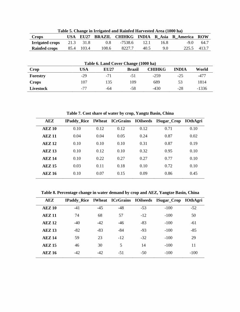
Table 5. Change in Irrigated and Rainfed Harvested Area (1000 ha)

Crops USA EU27 BRAZIL CHIHKG INDIA R_Asia R_America ROW

Irrigated crops 21.3 31.8 0.8 -7538.6 12.1 16.8 -9.0 64.7

Rainfed crops 85.4 103.4 108.6 8227.7 40.5 9.0 225.5 413.7

Table 6. Land Cover Change (1000 ha)

Crop USA EU27 Brazil CHIHKG INDIA World

Forestry -29 -71 -51 -259 -25 -477

Crops 107 135 109 689 53 1814

Livestock -77 -64 -58 -430 -28 -1336

Table 7. Cost share of water by crop, Yangtz Basin, China

AEZ IPaddy_Rice IWheat ICrGrains IOilseeds ISugar_Crop IOthAgri

AEZ 10 0.10 0.12 0.12 0.12 0.71 0.10

AEZ 11 0.04 0.04 0.05 0.24 0.87 0.02

AEZ 12 0.10 0.10 0.10 0.31 0.87 0.19

AEZ 13 0.10 0.12 0.10 0.32 0.95 0.10

AEZ 14 0.10 0.22 0.27 0.27 0.77 0.10

AEZ 15 0.03 0.11 0.18 0.10 0.72 0.10

AEZ 16 0.10 0.07 0.15 0.09 0.86 0.45

Table 8. Percentage change in water demand by crop and AEZ, Yangtze Basin, China

AEZ IPaddy_Rice IWheat ICrGrains IOilseeds ISugar_Crop IOthAgri

AEZ 10 -41 -45 -48 -53 -100 -52

AEZ 11 74 68 57 -12 -100 50

AEZ 12 -40 -42 -46 -83 -100 -61

AEZ 13 -82 -83 -84 -93 -100 -85

AEZ 14 59 23 -12 -32 -100 29

AEZ 15 46 30 5 14 -100 11

AEZ 16 -42 -42 -51 -50 -100 -100

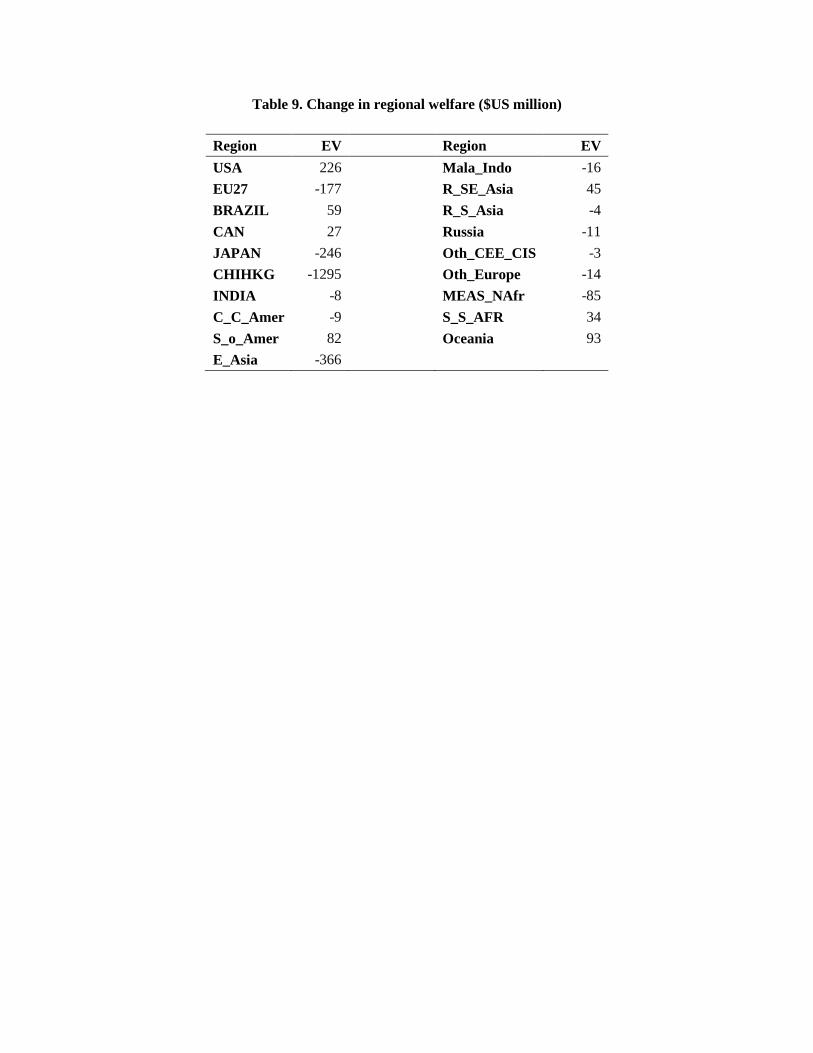
Table 9. Change in regional welfare ($US million)

Region EV Region EV

USA 226

Mala_Indo -16

EU27 -177

R_SE_Asia 45

BRAZIL 59

R_S_Asia -4

CAN 27

Russia -11

JAPAN -246

Oth_CEE_CIS -3

CHIHKG -1295

Oth_Europe -14

INDIA -8

MEAS_NAfr -85

C_C_Amer -9

S_S_AFR 34

S_o_Amer 82

Oceania 93

E_Asia -366

Figure 1. Nesting structure of water and land

Figure 2. Global share of water for irrigation and crop production

0

0.05

0.1

0.15

0.2

0.25

Glo

ba

l S

ha

re

Water use Irrigated crop output Total crop output

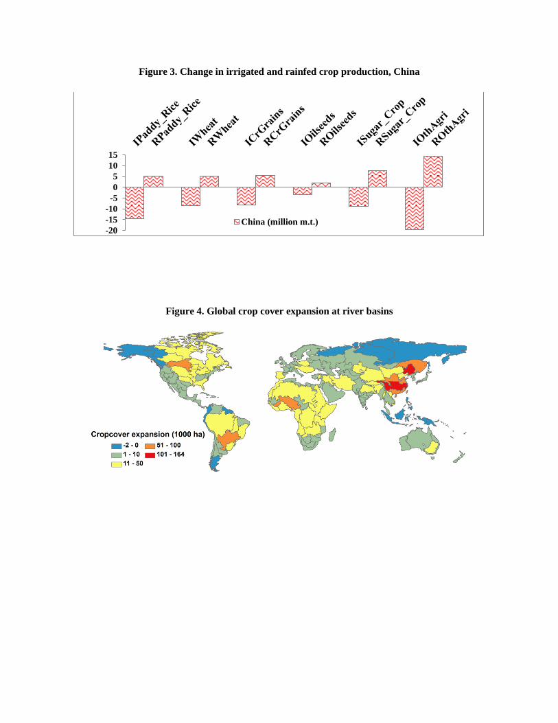
Figure 3. Change in irrigated and rainfed crop production, China

Figure 4. Global crop cover expansion at river basins

-20

-15

-10

-5

0

5

10

15

China (million m.t.)

Reference

Addams, L., G. Boccaletti, M. Kerlin, M. Stuchtey, and 2030 Water Resources Group and McKinsey and

Company. Charting Our Water Future: Economic Frameworks to Inform Decision-making. 2030

Water Resources Group, 2009.

Calzadilla, A., K. Rehdanz, and R.S.J. Tol. "The GTAP-W model: accounting for water use in

agriculture." Kiel Working Papers (Kiel Institute for the World Economy) 42, no. 3 (2011).

Calzadilla, A., K. Rehdanz, and R.S.J. Tol. "The GTAP-W model: accounting for water use in

agriculture." Kiel Working Papers (Kiel Institute for the World Economy), 2011.

de Fraiture, C., X. Cai, U. Amarasinghe, M.W. Rosegrant, and D. Molden. Does international cereal

trade save water? The impact of virtual water trade on global water use?Research Report-

Comprehensive Assessment of Water Management in Agriculture. International Water

Management Institute, 2004.

FAO. Agriculture, food and water. FAO, 2003.

FAO. Irrigation Management Transfer. FAO, 2007.

Pfister, S., P. Bayer, A. Koehler, and S. Hellweg. "Projected water consumption in future global

agriculture: Scenarios and related impacts." Science of the Total Environment 409, no. 20 (2011):

4206–4216.

Portmann, Felix T., Stefan Siebert, and Petra Döll. "MIRCA2000—Global monthly irrigated and rainfed

crop." GLOBAL BIOGEOCHEMICAL CYCLES, 2010: GB1011.1-GB1011.24.

Rosegrant, M.W., X. Cai, and S.A. Cline. World water and food to 2025: Dealing with scarcity.

International Food Policy Research Institute, 2002.

Siebert, S., and P. Döll. "Quantifying blue and green virtual water contents in global crop production as

well as potential production losses without irrigation." Journal of Hydrology 384, no. 3 (2010):

198--217.

Taheripour, F., T.W. Hertel, and J. Liu. "The Role of Irrigation in Determining the Global Land Use

Impacts of Biofuels." GTAP working paper series. 2011.

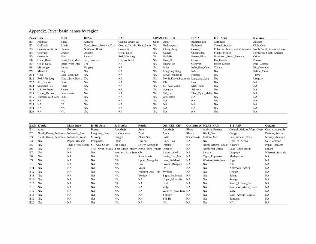
Appendix. River basin names by region

Basin USA EU27 BRAZIL CAN JAPAN CHIHKG INDIA C_C_Amer S_o_Amer

B1 Arkansas Baltic Amazon Canada_Arctic_At Japan Amur Brahmaputra Carribean Amazon

B2 California Britain North_South_America_Coast Central_Canada_Slave_Basin NA Brahmaputra Brahmari Central_America Chile_Coast

B3 Canada_Arctic_At Danube Northeast_Brazil Columbia NA Chang_Jiang Cauvery Cuba Carribean_Central_America North_South_America_Coast

B4 Colorado Dnieper Orinoco Great_Lakes NA Ganges Chotanagpui Middle_Mexico Northwest_South_America

B5 Columbia Elbe Parana Red_Winnipeg NA Hail_He Easten_Ghats Northwest_South_America Orinoco

B6 Great_Basin Iberia_East_Med San_Francisco US_Northeast NA Hual_He Ganges Rio_Grande Parana

B7 Great_Lakes Iberia_West_Atla Toc NA NA Huang_He Godavari Upper_Mexico Peru_Coastal

B8 Mississippi Ireland Uruguay NA NA Indus India_East_Coast Yucatan Rio_Colorado

B9 Missouri Italy NA NA NA Langcang_Jiang Indus NA Salada_Tierra

B10 Ohio Loire_Bordeaux NA NA NA Lower_Mongolia Krishna NA Tierra

B11 Red_Winnipeg North_Euro_Russia NA NA NA North_Korea_Peninsula Langcang_Jiang NA Uruguay

B12 Rio_Grande Oder NA NA NA Ob Luni NA NA

B13 Southeast_US Rhine NA NA NA SE_Asia_Coast Mahi_Tapti NA NA

B14 US_Northeast Rhone NA NA NA Songhua Sahyada NA NA

B15 Upper_Mexico Scandinavia NA NA NA Yili_He Thai_Myan_Malay NA NA

B16 Western_Gulf_Mex Seine NA NA NA Zhu_Jiang NA NA NA

B17 NA NA NA NA NA NA NA NA NA

B18 NA NA NA NA NA NA NA NA NA

B19 NA NA NA NA NA NA NA NA NA

B20 NA NA NA NA NA NA NA NA NA

Basin E_Asia Mala_Indo R_SE_Asia R_S_Asia Russia Oth_CEE_CIS Oth_Europe MEAS_NAfr S_S_AFR Oceania

B1 Amur Borneo Borneo Amudarja Amur Amudarja Rhine Arabian_Peninsul Central_African_West_Coast Central_Australia

B2 North_Korea_Peninsula Indonesia_East Langcang_Jiang Brahmaputra Baltic Amur Rhone Black_Sea Congo Eastern_Australi

B3 South_Korea_Peninsula Indonesia_West Mekong Ganges Black_Sea Baltic Scandinavia Eastern_Med East_African_Coast Murray_Australia

B4 NA Papau_Oceania Philippines Indus Dnieper Black_Sea NA Nile Horn_of_Africa New_Zealand

B5 NA Thai_Myan_Malay SE_Asia_Coast Sri_Lanka Lower_Mongolia Danube NA North_African_Coast Kalahari Papau_Oceania

B6 NA NA Thai_Myan_Malay Thai_Myan_Malay North_Euro_Russia Dnieper NA Northwest_Africa Lake_Chad_Basin Sahara

B7 NA NA NA Western_Asia_Iran Ob Eastern_Med NA Sahara Limpopo Western_Australia

B8 NA NA NA NA Scandinavia Iberia_East_Med NA Tigris_Euphrates Madagascar NA

B9 NA NA NA NA Upper_Mongolia Lake_Balkhash NA Western_Asia_Iran Niger NA

B10 NA NA NA NA Ural Lower_Mongolia NA NA Nile NA

B11 NA NA NA NA Volga Ob NA NA Northwest_Africa NA

B12 NA NA NA NA Western_Asia_Iran Syrdarja NA NA Orange NA

B13 NA NA NA NA Yenisey Tigris_Euphrates NA NA Sahara NA

B14 NA NA NA NA NA Upper_Mongolia NA NA Senegal NA

B15 NA NA NA NA NA Ural NA NA South_African_Co NA

B16 NA NA NA NA NA Volga NA NA Southeast_Africa_Coast NA

B17 NA NA NA NA NA Western_Asia_Iran NA NA Volta NA

B18 NA NA NA NA NA Yenisey NA NA West_African_Coastal NA

B19 NA NA NA NA NA Yili_He NA NA Zambezi NA

B20 NA NA NA NA NA NA NA NA NA NA