1

War Inc. or Peace Inc.? Firms, War and Political Micro-Economy of International Conflict*

By

Isa Camyar , PhD Bahar Ulupinar, PhD

International Relations Program Department of Economics and Finance

University of Pennsylvania West Chester University

652 Williams Hall, 255 S. 36th Street 304 Anderson Hall

Philadelphia, PA, 19104 West Chester, PA 19383

Phone: +1 215 898 0452 Phone: +1 610 436-3468

E-mail: icamyar@sas.upenn.edu E-mail: bulupinar@wcupa.edu

Abstract:

This research explores the microeconomic consequences of war. In particular, we examine the impact of war on firm profitability. Building on a two-sector dynamic general equilibrium model and using a wealth of insights in the literature on war and economy, we develop a set of hypotheses about the systemic, sectoral, short-term and long-term impacts of war on firm profitability. Our empirics utilize a panel dataset with more than 15,000 firms in the United States (US) for the period from 1960 to 2007, and probe how US government’s war involvement impacts US firms’ profitability. Our preliminary results based on single-equation error-correction models show that (a) on balance war hurts firm performance; (b) war impact on profitability in the defense sector is surprisingly weak; and (c) the short-term impact of war is more robust than its long-term impact. Collectively, our results hint that war is likely to influence firm performance mainly via the size and quality of firms’ productive technologies.

Keywords:

War, Firms, Profitability, Political Micro-Economy

*Prepared for presentation at the 2012 annual meeting of the International Political Economy Society (IPES), University of Virginia, November 9-10. Any comments and suggestions would be most welcome.

2

War or its prospect is ubiquitous in international relations. One aspect of this phenomenon that

remains to be fully understood is its economic consequences. Since the economic impact of war

is more than merely a scholarly interest, but also a key consideration in policy-makers’ decision

to use armed force, a sizable body of literature has arisen to probe it. Our research contributes to

this literature in at least two ways.

First, we study the impact of war on a specific subset of economic actors: firms. In particular,

our analysis examines the impact of war on firms’ operational performance. A focus on firms

sets us apart from most studies in the literature, which investigate the impact of war on macro

variables like growth, trade and investment (Organski & Kugler, 1977, Rasler & Thompson,

1985; Collier, 1999; Barbieri & Levy. 1999; Koubi, 2005; Kang, Seonjou and James Meernik,

2005). Along with its intrinsic value, firm performance is worthwhile to study for two other

reasons. First, in modern societies, firm economic behavior has considerable implications for the

achievement of many socially desirable outcomes like employment, innovation, environmental

protection. Consequently, identifying war impact on firm performance can enrich our general

understanding of how war affects a wider range of outcomes. Second, firms are among principal

political actors in modern politics. Knowing how war impacts firms can shed some light into

their preferences and behavior in the domestic politics of war and peace. Overall, our research

contributes to advance the general understanding of the political micro-economy of war.

Second, we offer a multifaceted view of war impact on firms by flashing out its systemic,

sectorial, short-run and long-run aspects. A focus on these multiple aspects in the same

theoretical and empirical framework differentiates us from those few studies that link war to firm

performance. Studies like Abadie and Gardeazabal (2003), Guidolin and La Ferrara (2007)

explore the impact of war on sectors or firms whose income is affected by a development in a

3

war region and whose stocks are traded within a particular market with some sensitivity to armed

conflict. However, these studies do not explicitly distinguish systemic from sectoral or short-

term from long-term impacts, when it is made clear by other studies that war has sector-specific

as well as systemic impacts, which are distributed over time. We use a two-sector general

dynamic equilibrium model to sort out general theoretical implications about the multiple aspects

of war impact on firms and then implement the error correction model to test these implications.

We study the firm-level consequence of war with a panel dataset of more than 15,000 US

firms from 1960 to 2007. Our empirics probe how the war involvement of US government

influences the operational performance of US firms. Our focus on US is driven in part by our

methodological considerations. There are extensive financial and accounting data on a

substantial number of US firms over a large span of time. Also, a single-country focus has some

methodological advantages like avoiding country-level heterogeneity and keeping relatively

constant some institutional and legal determinants of firm performance like regime type and

legal system that are not of primary interest here.

Our preliminary results show that (a) on balance, the profitability of US firms declines due to

US government’s war involvement in both short and long-terms; (b) war impact on profitability

in the defense sector is surprisingly weak; and (c) the short-term impact of war, systemic or

sectoral, is much more robust than its long-term impact.

In what follows, we first present a two-sector dynamic equilibrium model and discuss the

relevant literature to develop expectations about the connection between war and firm

performance. In our empirics, we execute the single-equation error correction model. The last

section wraps up the discussion.

4

THEORY AND HYPOTHESES

Prior research establishes that war activates multiple and, sometimes, conflicting economic

forces. On the one hand, war (a) destroys human and physical capital; (b) dislocates resources

from their productive uses; (c) disrupts economic exchanges by increasing uncertainty and

transaction costs. On the other, war (a) can activate a positive demand shock via increased

government spending; and (b) can spur a positive technology shock by contributing to the

innovation and adoption of new technologies. In order to identify how these multiple forces feed

into firm performance, we first offer a stylized representation of how the economy works.

Following Ramey & Shapiro (1998a) and Rogerson (1987), we present a two-sector dynamic

general equilibrium model. While we largely maintain their underlying intuitions and the aspects

of their specifications, the model reflects our particular interest in the micro-economic

consequences of war. In the model, the economy consists in two sectors: defense (DS) and

civilian (CS) sectors. Given our analytical interest, such a distinction is proper. In each sector,

firms produce with the standard Codd-Douglas production technology. Different from Ramey &

Shapiro (1998a, 1998b) and similar to studies like Barth and Cordes (1980), Aschauer (1988)

and Ramirez (1994), we add public capital as a separate input into the conventional Codd-

Douglas technology. The augmented Codd-Douglas production technology is as follows:

Yit= AKα

itLyitKG

ßt i=1, 2 (1)

where Yit is the flow of output in sector i and during period t; A is a scale parameter; Kit is the

stock of available private capital in sector i during period t with α being the marginal product or

the output elasticity of Kit; Lit is labor employed in sector i during period t with y being the

5

marginal product of Lit; KGt is the stock of publicly provided fixed capital services1 during

period t with ß being the marginal product of KGt. This production technology is characterized

with constant returns to scale. That is, a proportional rise in productive factor is assumed to raise

Y by the same proportion (i.e. α + y + ß=1).

A key premise in our model is that there are frictions in capital and labor reallocation across

sectors. That is, there are time and utility costs in shifting K and L across sectors. This premise is

backed up by numerous empirical studies and shared by various formalizations of the economic

impact of sector-specific shocks (Lilien 1982; Ramey & Shapiro, 1998b; Kambourov, Gueorgui,

2009).The premise is particularly proper in our case because war presumably prompts sector-

specific preference shocks. The assumed frictions in labor and capital reallocation can help

explain how these shocks propagate across sectors and persist over time.

Firms in each sector can add to their capital stocks by buying either newly-produced

investment goods within the sector or used capital from the other sector. New capital is

productive only one period after it is produced. In order to shift across sectors, used capital must

spend one period being unproductive. In other words, there is a delay in adjusting K in each

sector when the sector faces a preference shock. Furthermore, there is some loss in K when it

shifts sector. That is because some characteristics of private capital from one sector is not fully

valued in the other sector. The following equations represent how the stock of private capital

evolves in each sector:

1 Here public fixed capital refers to core infrastructure including highways, airports and mass

transit facilities, electric and gas plants, water supply facilities and sewers, and also buildings

including schools, hospitals, police and fire stations, courthouses, garages and passenger

terminals, all of which contribute to an orderly environment that facilitates private production.

6

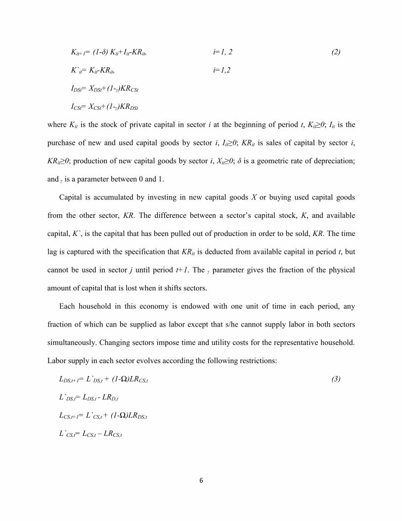
Kit+1= (1-δ) Kit+Iit-KRit, i=1, 2 (2)

K`it= Kit-KRit, i=1,2

IDSt= XDSt+(1-ᵧ)KRCSt

ICSt= XCSt+(1-ᵧ)KRDSt

where Kit is the stock of private capital in sector i at the beginning of period t, Kit≥0; Iit is the

purchase of new and used capital goods by sector i, Iit≥0; KRit is sales of capital by sector i,

KRit≥0; production of new capital goods by sector i, Xit≥0; δ is a geometric rate of depreciation;

and ᵧ is a parameter between 0 and 1.

Capital is accumulated by investing in new capital goods X or buying used capital goods

from the other sector, KR. The difference between a sector’s capital stock, K, and available

capital, K`, is the capital that has been pulled out of production in order to be sold, KR. The time

lag is captured with the specification that KRit is deducted from available capital in period t, but

cannot be used in sector j until period t+1. The ᵧ parameter gives the fraction of the physical

amount of capital that is lost when it shifts sectors.

Each household in this economy is endowed with one unit of time in each period, any

fraction of which can be supplied as labor except that s/he cannot supply labor in both sectors

simultaneously. Changing sectors impose time and utility costs for the representative household.

Labor supply in each sector evolves according the following restrictions:

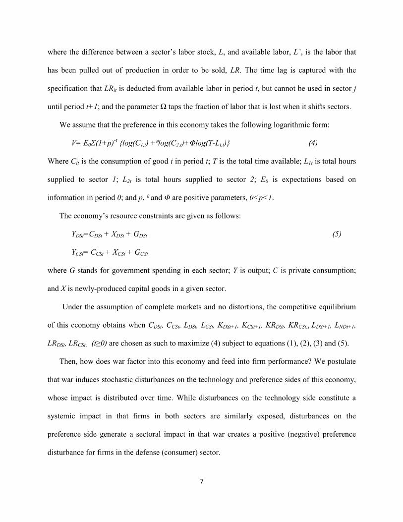
LDS,t+1= L`DS,t + (1-Ω)LRCS,t (3)

L`DS,t= LDS,t - LRD,t

LCS,t+1= L`CS,t + (1-Ω)LRDS,t

L`CS,t= LCS,t – LRCS,t

7

where the difference between a sector’s labor stock, L, and available labor, L`, is the labor that

has been pulled out of production in order to be sold, LR. The time lag is captured with the

specification that LRit is deducted from available labor in period t, but cannot be used in sector j

until period t+1; and the parameter Ω taps the fraction of labor that is lost when it shifts sectors.

We assume that the preference in this economy takes the following logarithmic form:

V= E0Σ(1+p)-t log(C1,t) +ᶿlog(C2,t)+Φlog(T-Li,t) (4)

Where Cit is the consumption of good i in period t; T is the total time available; L1t is total hours

supplied to sector 1; L2t is total hours supplied to sector 2; E0 is expectations based on

information in period 0; and p, ᶿ and Φ are positive parameters, 0<p<1.

The economy’s resource constraints are given as follows:

YDSt=CDSt + XDSt + GDSt (5)

YCSt= CCSt + XCSt + GCSt

where G stands for government spending in each sector; Y is output; C is private consumption;

and X is newly-produced capital goods in a given sector.

Under the assumption of complete markets and no distortions, the competitive equilibrium

of this economy obtains when CDSt, CCSt, LDSt, LCSt, KDSt+1, KCSt+1, KRDSt, KRCSt,, LDSt+1, LNDt+1,

LRDSt, LRCSt, (t≥0) are chosen as such to maximize (4) subject to equations (1), (2), (3) and (5).

Then, how does war factor into this economy and feed into firm performance? We postulate

that war induces stochastic disturbances on the technology and preference sides of this economy,

whose impact is distributed over time. While disturbances on the technology side constitute a

systemic impact in that firms in both sectors are similarly exposed, disturbances on the

preference side generate a sectoral impact in that war creates a positive (negative) preference

disturbance for firms in the defense (consumer) sector.

8

Systemic Impact of War

War induces a disturbance in the size and quality of productive technologies available to firms in

both sectors, the full impact of which materializes over time. In the short term, the destruction of

human (L) and private capital (K) diminishes the economy-wide stock of productive resources

available to all firms and puts a downward pressure on firms’ productive capability and output

(Y). Furthermore, a war-related destruction of the public capital stock freely available to firms in

both sectors is expected to engender a negative impact on output in both sectors. Assuming that

KG is productive (ß>0) and complements the private capital stock and labor, the destruction of

KG (a) directly decreases output; (b) indirectly reduces the marginal productivity of K; and (c)

indirectly decreases the marginal productivity of labor due to the decline in the amount of capital

per worker. Furthermore, war leads to the dislocation of resources from productive use in the

short-term. For example, resources used for public investment are now used for war efforts,

setting the same chain reaction as in the destruction of KG, which further depresses firms’

productive capability and output. In addition, a war-induced uncertainty in the business

environment can preclude mutually advantageous transactions, which further limits the efficient

allocation of productive resources.

Hypothesis (1): All else being equal, war has a negative short-term systemic impact on firm

performance.

Unlike the short term, however, war is likely to generate conflicting forces on firms’

productive capability in the long term. On the one hand, studies document that a positive

technological spinoff is likely to arise from war experience for at least three reasons. First, new

technologies with commercial application can be developed in war-motivated research and

development efforts (Ruttan, 2006). Second, war leads to the destruction of obsolete

9

infrastructure and technologies which can be replaced with more efficient ones, an idea captured

in the Phoenix factor (Organski & Kugler, 1980; Kugler & Arbetman, 1989). Third, war can

destroy the institutional sclerosis behind technological progress due to the influence of

entrenched distributional coalitions, which are shown to slow down the adoption of new

technologies (Olson, 1982; Chan, 1987). On the other, if war overhang arises due to the

persistent dislocative impact of war, there could be a downward pressure on the stock of

productive resources for firms in both sectors for some times. In fact, evidence is vast that the

portion of public sector expansion and an increase in military allocation due to war efforts hardly

returns to its prewar level, suggesting that the disruptive impact of war on the efficiency of

resource allocation persists at least some time (Peacock & Wiseman, 1961; Russett, 1970; Diehl

& Goertz, 1985).

In sum, there are theoretical and empirical reasons to expect that war can depress or stimulate

firms’ output by generating negative or positive disturbances in their productive technology.

Therefore, the net long-term impact of war is not theoretically unambiguous. Therefore, we

derive the following nondirectional hypothesis:

Hypothesis (2): All else being equal, war has a long-term systemic impact on firm

performance.

Sectoral Impact of War

War also generates sector-specific preference shocks. Just like the systemic impact, the sectoral

impact is also distributed over time. In the short-run, firms in the civilian sector are expected to

experience a negative demand shock due to an expected decline in private consumption (Ccs) and

investment (Xcs) spending. Since the negative short-term systemic effect is likely to reinforce

10

rather than counter the effect due to a negative demand shock and resource release, we derive the

following directional hypothesis

Hypothesis (3a): All else being equal, war has a negative short-run impact on firm

performance in the civilian sector.

Firms in the defense sector, on the other hand, experience a positive preference shock with an

increased government demand for their products (GDS). A general decline of private consumption

(CDS) should not impact these firms as strongly as firms in the civilian sector because the

government is the primary purchaser of goods from the defense sector. While the short-term

impact on firms in the defense sector seems obvious, our theoretical model suggests that it is not

all that straightforward. There is a possibility that the short-term sectoral impact on firms in the

defense sector can be weak. That is so for two reasons. First, frictions in capital and labor

reallocation across sectors can mitigate the initial positive preference shock for firms in the

defense sector. In other words, there might be some delays in matching productive capabilities

with an increased demand, which mitigates the expectedly positive impact of the demand shock.

Second, the negative short-run systemic effect can potentially neutralize the positive demand

shock. As a result, we reach to the following nondirectional hypothesis:

Hypothesis (3b): All else being equal, war has a short-term impact on the performance of

firms in the defense sector.

In the long term, while the sector-specific disturbances are expected to wane, frictions in

labor and capital reallocations may lead to its persistence. Firms in the civilian sector are likely

to continue to experience a downward pressure on their performance for a while even if the

negative demand shock recedes. However, the long-term systemic effect can either reinforce or

offset this negative sectoral effect. If the long-term systemic effect is positive due to the

11

technological spinoff, it counters the negative long-run sectoral impact. However, if the long-run

systemic effect is negative due to the persistence of war’s dislocative effect or war overhang, it

reinforces the negative long-run sectoral impact. Given this ambiguity, we specify the following

non-directional hypothesis:

Hypothesis (4a): All else being equal, war has a long-term impact on firm performance in the

civilian sector

Firms in the defense sector, on the other hand, are likely to experience a positive long-term

impact arising from war for two reasons. First, the technological innovation due to war efforts is

likely to be felt much earlier and strongly for firms in the defense sector. Therefore, the positive

systemic effect of war via technological innovation-adoption is likely to be much more

pronounced for these firms than for firms in the civilian sector. Second, the dislocative impact of

war especially in the form of persistence in higher military allocation does not necessarily hurt

these firms as a favorable demand schedule persists. As a result, it is conceivable to derive the

following directional hypothesis:

Hypothesis (4b): All else being equal, war has a positive long-term effect on firms in the

defense sector.

VARIABLES AND DATA

To assess the firm-level consequences of war, we use a sample that is drawn from the

universe of firms appearing in Compustat between years 1960 and 2007. Compustat provides

annual, firm-level balance sheet, income statement and cash flow information for active and

inactive publicly-held companies since 1960. Our sample has 144,516 firm-year observations.

Our dependent variable is firm performance. We operationalize this variable as Profitability

and measure it as Earnings before Interests and Taxes (EBIT), scaled by total assets. Our key

12

independent variable is US involvement in a war (War). We use the Version 4 of the Correlates

of War (COW) data to identify the wars that the US was actively involved for each given year

since 1960. The COW project classifies wars into three categories: interstate, intrastate and

extrastate wars. Interstate war refers to wars between or among states (members of the interstate

system).For example, the first Gulf war was an example of interstate war. Intrastate war refers to

wars that that predominantly takes place within the recognized territory of a state. An example

would the US involvement in the Somalian conflict from 1992 to 1994. Extrastate wars are the

ones that take place between a state (s) and a nonstate entity outside the borders of the state. For

example, the wars in Afghanistan and Iraq are classified as extrastate wars, because these wars

were waged in part against nonstate entities: Al-Qaeda and Iraqi resistance in the Iraqi war, and

Al-Qaeda and Taliban in the Afghan war.

War is a count variable or the total number of interstate, intrastate and extrastate wars that the

US is involved in a given year. Table 1 provides the list of all international wars that the US was

involved during our time frame. In particular, the US was part of a total of 19 wars (7 interstate

wars, 10 intrastate wars and 2 extrastate wars). Out of 47 years that our analysis covers, the US

was involved in some form of war during 28 years. While the 1960s and 2000s were the most

violent decades, the 1980s was the most peaceful one.

[Table 1 about here]

In testing the sectoral impact of war, we use Defense, a dummy variable that is equal to “1” if

a firm belongs to one of the following industries, “0” otherwise: gun2, shipbuilding

3 and aircraft

4.

2 Firms with the following standard industry classification numbers (sicnum): sicnum ge 3760

and sicnum le 3769; sicnum ge 3795 and sicnum le 3795; sicnum ge 3480 and sicnum le 3489

13

Our analysis includes a number of control variables. Some of these variables are at the firm

level. Size (the natural logarithm of market capitalization, which is the shares outstanding times

closing stock price at the end of a fiscal year) taps the influence of firm size on profitability.

Following studies like Allayannis and Weston (2001), Brockman and Unlu (2009), Ferreira and

Matos (2008), and Anderson and Reed (2003), Leverage (the sum of long term debt and short

term debt, scaled by the sum of book value of equity plus long term debt and short term debt),

Dividend (total dividend payment scaled by sales) and Cash (cash or cash equivalents held by a

firm scaled by sales) are used to tap a firm’s financial health. Furthermore, a firm’s profitability

may be related to its growth prospects (Anderson and Reeb, 2003). Consequently, we include

Capital (fixed capital expenditures scaled by sales) and R&D (Research and development

expenditures scaled by sales) to tap a firm’s growth prospects. We winsorize all the firm-level

controls at their 1th and 99th percentile values to reduce the influence of extreme values.

In addition, our analysis includes a series of aggregate level factors. To capture the stage of

the business cycle, we include ln(GDP), GDP Growth and Inflation. The data for these variables

are drawn from the Penn Worl Table. Cold War is a pertinent background factor. Democrat is

necessary to include as prior research shows that the partisan orientation of the president colors

the choice of macroeconomic policies, which further influence firms’ overall business

environment (Hibbs, 1977). Since some of these factors can conceivably impact both firm

3 Firms with the following standard industry classification numbers (sicnum): sicnum ge 3730

and sicnum le 3731; sicnum ge 3740 and sicnum le 3743

4 Firms with the following standard industry classification numbers (sicnum): sicnum ge 3720

and sicnum le 3720; sicnum ge 3721 and sicnum le 3721sicnum ge 3723 and sicnum le 3724;

sicnum ge 3725 and sicnum le 3725; sicnum ge 3728 and sicnum le 3729

14

profitability and war, their inclusion is necessary to establish the genuineness of the relationship

between War and Profitability. For example, the state of economy can determine not just firm

profitability but also the likelihood of war as discussed in prior research (Russett, 1990;

DeRouen, 1995). In the same vein, the partisan orientation of the president can determine not just

general macroeconomic policies and hence firm performance, but also the US’s propensity to

engage in a war (Ostrom and Job, 1986; Lian and Oneal, 1993).

ANALYSIS AND RESULTS

Our empirical analysis represents the effect of war on firm profitability in the form of an error

correction model. The setup of this model is able to capture both short-term and long-term

effects, as well as diagnosing negative and positive feedback processes that give rise to either

equilibrium or disequilibrium. Since we postulate that while some consequences of war occur

more or less contemporaneously, others are distributed over time such that the full effect

materializes over time, this model is proper in our case.

More specifically, we estimate the short and long-term effects of War on Profitability using

the single equation method. This strategy is selected over the most common alternative, the

Engle-Granger two-step model (Engle and Granger, 1987), due to its applicability in a wider

range of circumstances. Unlike the two-step method, the single equation model does not impose

the assumption of cointegration on the series analyzed. In fact, the single equation error-

correction model is a modified version of an autoregressive distributed lag model in which the

dependent variable is a function of its past values and past values of the independent variables.

This is an important advantage for two reasons. First, the presence of cointegration in political

relationships remains contentious, while reliance upon the Engle-Granger two-step procedure has

been shown to be problematic (De Boef and Granato 1999). Second, most diagnostic tests for

15

unit root possess low power against local alternatives (De Boef and Granato 1997, 1999),

meaning it tends to be difficult to ascertain whether series are (co)integrated with confidence.

Furthermore, this framework is appropriate for modeling feedback and equilibrium relationships

in stationary as well as nonstationary data (Banerjee, Dolado, and Galbraith 1993; Davidson and

MacKinnon 1993; De Boef and Keele 2008). This analysis therefore specifies the dynamic and

equilibrating relationship between war and profitability in the form of the following single-

equation error-correction model:

∆Profitabilityi,t= α+ß∆Wari,t+Φ(Profitabilityi,t-1-Wari,t-1ƴ) + εi,t (6)

where Profitability is the dependent variable, the performance of firm i at time t; War is

the independent variable; the error correction mechanism, (Profitabilityi,t-1 - Wari,t-1ƴ),

measures how far out of equilibrium the dependent and independent variables vary

following short-term changes, and the parameter Φ captures how quickly the relationship

returns to equilibrium.

In practice, we augment equation (6) by adding other control variables and rewrite it in two

different forms. To capture the systemic effect of War, we estimate the following model:

∆Profitabilityi,t= α+ ß0Profitabilityi,t-1+ ß1∆Wari,t+ ß2Wari,t-1+ ßControls+ δ+ Ω

+ εi,t (7)

Where ß1 captures the short-term systemic effect of War; ß2 captures the long-term systemic

effect of War. ß0 captures as the same thing as Φ in equation (6) and represents the error

correction rate.

To capture the sectoral effect of War, we estimate the following model:

16

∆Profitabilityi,t= α+ ß0Profitabilityi,t-1+ ß1a∆Wari,t + ß2Wari,t-1 +

ß3∆Wari,t*Defenset + ß4Wari,t-1*Defencet+ ß5Defence + ßControls+ δ+ Ω + εi,t

(8)

where ß1 captures the short-term effect of War on profitability in the civilian sector; ß2 taps the

long-term effect of War on profitability in the civilian sector; ß3 taps the short-term impact of

War on profitability in the defense sector; ß4 is the long-term impact of War on profitability in

the defense sector; ß5 captures the impact on profitability in the defense sector when there is no

conflict; and ß0 is the error correction rate.

In both models, δ, dummy variables for all years except one, accounts for common

unobserved shocks to all firms in a particular year such as global energy shocks; Ω, dummy

variables for all industries except one, taps industry-specific unobserved fixed effects.

Furthermore, the clustered nature of our data creates heterogeneity in our errors terms. Therefore,

we use robust standard errors to alleviate this problem. Also, we cluster standard errors by firm

to account for the fact that the residuals of a given firm may be correlated across years

generating downwardly biased standard errors and hence making the rejection of the null

hypothesis much easier.

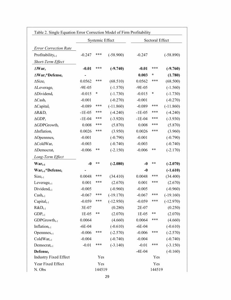
Our main results are presented in Table 2. The short-term parameter of the systemic model

indicates that there is a contemporaneous effect of war on firm profitability, significant at

p<0.00. This confirms Hypothesis (1). As a war breaks out, it generates a negative technology

shock that influences all firms regardless of their sector affiliation and puts a downward pressure

on their profitability. However, the long-run parameter of the systemic model shows that even

after a significant negative shock, firm profitability is still too high compared to the distance

between War and Profitability when in their equilibrium state. The coefficient for the lagged

17

value of War highlights that profitability declines by 0.003 to correct the disturbance to the long-

term relationship. The error correction rate indicates that about 25 % of this equilibration effect

will be realized the year after a change in war. Overall, it takes more than 10 years after the

initial shock to correct the disequilibrium. This suggests that there is a significant war overhang

effect on firm profitability, which persists over a considerable time.

[Table 2 about here]

The short-term parameters of the sectoral model confirm both Hypotheses 3a and 4a. Recall

that while the coefficient for ∆War captures war impact on firm profitability in the consumer

sector, the coefficient for ∆War*Defense taps the impact on profitability in the defense sector.

Our model estimation identifies a strong negative contemporaneous impact on profitability in the

consumer sector in line with Hypothesis 3a. On the other hand, war has a positive

contemporaneous impact on profitability in the defense sector. However, it is important to note

that this impact is barely significant (p=0.073). In other words, the negative short-term impact in

the consumer sector is more significant than the positive impact in the consumer sector both

statistically and substantively. Although a war-induced positive preference shock boosts the

profitability of firms in the defense sector, it does not do so as strongly as conventionally

assumed. How to interpret this result? According to our theoretical model, this may be due to

delays in the sectoral impact of war that stem from frictions in capital and labor reallocations.

Additionally, it is conceivable that while the negative systemic effect reinforces the negative

preference shock for firms in the consumer sector, it is likely to offset the positive preference

shock for firms in the defense sector.

The long-term parameters of the sectoral model reveal some interesting patterns. The

coefficient for War highlights that while the initial shock of war depresses firm profitability in

18

the civilian sector, profitability is still too high, and consequently needs to go down some more

as the full effect of war realizes. However, the coefficient for War*Defence is not significant,

suggesting that the effect of war in the defense sector is felt quickly and fully captured in the

short-term. Again, this result can be explained in part by frictions in factor reallocation across

sectors. Although, in the long-run, a war-induced preference shock is expected to wane,

according to our theoretical model, this may not happen right away or take time. This would

explain why the negative impact in the consumer sector persists at least for some times.

How robust are the results reported thus far? In order to test the stability of our results, we

run two sets of additional analysis. First, we investigate whether the type of war matters. In the

preceding discussion, we aggregate all three forms of war into one indicator. However, it is

pertinent to test the differential impacts of interstate, intrastate and extrastate wars on firm

profitability. Accordingly, we use Interstate, Intrastate and Extrastate as the total number of

interstate, intrastate and extrastate wars that the US was involved in a given year, respectively.

The results for different types of war are presented in Table 3. All the short-term parameters

of the system model are significant, indicating that all wars regardless of type induce a negative

shock for firm profitability. However, the long-term parameters are insignificant with the

exception of the parameter for Intrastate. On the side of the sector model, while the short-term

parameters for the civilian sector are all negative and significant, the two parameters for the

defense sector are not significant. In the long run, none of the parameters for either the defense

sector or the civilian sector is significant. The results jointly underline the relative weakness of

war impact for the long-term and the defense sector.

[Table 3 about here]

19

Second, it is incumbent to test whether our results vary according to war characteristics. As a

result, we run our systemic and sectoral models with indicators of three war characteristics:

duration, severity and proximity. Duration is the number of days in a given year that the United

State was actively engaged in a conflict. Severity is the total number of battlefield casualties per

day. Duration and Severity jointly capture the destructiveness of war experience. Additionally, in

the spirit of studies like Murdoch and Todd Sandler (2002, 2004), which identify a spatial aspect

of war economic impact, we use two indicators for the proximity of a war. While the first

indicator, PProximity, captures the physical proximity of the location of a war to the US

homeland, the second indicator, FProximity, taps the functional proximity of the location of a

conflict. PProximity is the average number of miles from the location of a conflict(s) in a given

year. In cases of multiple wars for a given year, the average distance is used. FProximity is the

trade that the US had with the region where a war happened at the time of the war as a

percentage of US total trade. In cases of multiple wars for a given year, the total trade with the

war regions as a percentage of US total trade is used.

Table 4 presents the results for war characteristics. In the systemic model, both the short term

and the long-term parameters for Duration and Severity are negative and significant. As the

destructiveness of war experience grows, firm profitability becomes more depressed in both the

short-term and the long-term. While the results for physical proximity (PProximity) are not

significant, the results for functional proximity (FProximity) are positive and significant. Wars in

regions where US have strong economic stakes do not hurt firm profitability. On contrary, those

wars boost the profitability of US firms in both the short-term and the long-term. In the sectoral

model, the impact of war characteristics is much more pronounced for the civilian sector than for

the defense sector.

20

[Table 4 about here]

DISCUSSION

Collectively, our preliminary results point to the following patterns. First, the systemic

impact of war is more robust than its sectoral impact. On balance, war depresses firm

profitability regardless of industry affiliation. Second, there is a notable variation across sectors

in terms of the magnitude and significance of war impact. In general, the expectedly negative

impact on the consumer sector is much more robust than the expectedly positive impact on the

defense sector. Third, the short-term impact of war, whether sectoral or systemic, is much

stronger than its long-term impact. That is, a substantial portion of war impact on firms

materializes in the short-term, even though there seems to be a significant long-term effect.

Then, the pertinent question is exactly what drives our results. In our theoretical discussion,

we postulate that war impact on firms arises through technology and preference shocks.

Although further analysis is needed, we have at least two reasons to suppose that the war impact

reported here may operate more through technology shocks than preference shocks. First, in our

theoretical model, while the systemic effect derives from technology shocks, the sectoral effect is

driven by preference shocks. The relatively more robust systemic effect hints that the war impact

via technology shocks is stronger than the war impact via preference shocks. Second, some of

our aggregate controls like GDP, GDP Growth and Inflation, which are intended to capture the

stage of the business cycle in the US economy, also taps the preference side of the economy.

While these controls would also account for part of war-induced technology shocks, they are

more likely to cover war impact via war-induced preference shocks.

Even if technology shocks seem to drive our significant results, there is still a question of

exactly how these shocks might have operated in our sample. One general observation about the

21

wars involving US during our time frame is that none of them led to a massive destruction of

capital and labor, partly because they were fought in distant lands. Therefore, it is probably not

the physical destruction of economic factors that drive our results. However, it is conceivable

that these wars might have led to the dislocation of resources from their productive use.

Particularly important is the impact of war on public investment. If there had been a war-induced

short-term and long-term decline in public investment and hence the stock of public capital, this

would have the same impact as the destruction of public capital.

In sum, the results of our preliminary analysis suggest that war hurts firm performance.

However, additional analysis is needed to (a) do further testing of the stability of our results, (b)

shed more light into the causal mechanisms driving our main results; and (c) elaborate more on

the surprisingly weak results for the defense sector.

22

APPENDIX: CORRELATION MATRIX

Variables

(1) (2) (3) (4) (5) (6) (7) (8) (9) (10) (11) (12) (13) (14) (15)

Profitability (1)

1.00

War (2)

-0.04 1.00

Size (3)

0.20 0.13 1.00

Leverage (4)

-0.01 0.00 -0.01 1.00

Dividend (5)

0.01 0.03 0.10 0.00 1.00

Cash (6)

-0.30 0.12 0.02 -0.02 -0.03 1.00

Capital (7)

0.05 -0.07 0.02 0.00 -0.08 -0.08 1.00

R&D (8)

0.02 0.02 0.22 0.00 -0.01 0.01 -0.01 1.00

GDP (9)

-0.26 0.21 0.28 0.00 0.03 0.25 -0.13 0.07 1.00

GDP Growth (10)

0.03 0.02 0.01 0.00 0.01 0.00 0.02 -0.01 -0.10 1.00

Inflation (11) 0.19 -0.15 -0.23 0.00 -0.04 -0.18 0.09 -0.04 -0.57 -0.31 1.00

Openness (12)

-0.28 0.22 0.28 0.00 0.03 0.25 -0.12 0.07 0.99 -0.08 -0.59 1.00

Cold War (13)

0.25 -0.19 -0.25 0.00 -0.02 -0.23 0.11 -0.06 -0.86 -0.02 0.66 -0.89 1.00

Democrat (14)

0.00 -0.30 0.01 0.00 -0.01 0.02 0.04 -0.01 -0.06 0.33 -0.20 0.03 -0.27 1.00

Defence (15)

0.02 0.01 0.01 0.00 -0.02 -0.02 -0.02 0.02 -0.04 0.01 0.02 -0.04 0.04 0.00 1.00

23

REFERENCE

Abadie, Alberto, and Javier Gardeazabal. 2003. “The Economic Costs of Conflict: A

Case Study of the Basque Country.” American Economic Review, 93(1): 113-132.

Allayannis, George and James P. Weston. 2001. “The Use of Foreign Currency

Derivatives and Firm Market Value.” Review of Financial Studies, 14(1): 243-76.

Anderson, Ronald C., and David M. Reeb. 2003. “Founding-Family Ownership and

Firm Performance: Evidence from the S&P 500.” Journal of Finance, 58(3): 1301-

1328.

Aschauer, David A. 1988. “Government Spending and the Falling Rate of Profit.”

Economic Perspectives, 6: 11-17.

Banerjee, Anindya, Juan J. Dolado, and John W. Galbraith. 1993. Integration, Error

Correction, and the Econometric Analysis of Non-Stationary Data. Oxford: Oxford

University Press.

Barbieri, Katherine, and Jack S. Levy. 1999. “Sleeping with the Enemy: The Impact of

War on Trade.” Journal of Peace Research, 36 (4): 463-79.

Barth, James R. and Joseph Cordes. 1980. “Substitutability. complementarity, and the

impact of government spending on economic activity.” Journal of Economics and

Business, 32(3), 235-42.

Brockman, Paul, and Emre Unlu. 2009. “Dividend Policy, Creditor Rights, and the

Agency Cost of Debt.” Journal of Financial Economics, 92: 276-99.

Chan, Steve. 1987. “Growth with Equity: A Test of Olson's Theory for the Asian

Pacific Rim Countries.” Journal of Peace Research, 24(2): 135-149.

24

Collier, Paul, 1999. “On the Economic Consequences of Civil War.” Oxford Economic

Papers, 51(1): 168-183.

Diehl, Paul, and Gary Goertz. 1985. “Trends in Military Allocations Since 1816: What

Goes Up Does Not Always Come Down.” Armed Forces and Society 12(1): 134-

144.

Ferreira, Miguel A., and Pedro Matos. 2008. “The Color of Investors’ Money: The Role

of Institutional Investors around the World.” Journal of Financial Economics, 88:

499–533.

Guidolin, Massimo, and Eliana La Ferrara. 2007. “Diamonds Are Forever, Wars Are

Not: Is Conflict Bad for Private Firms?” American Economic Review, 97(5): 1978-

1993.

Davidson, Russell, and James G. MacKinnon. 1993. Estimation and Inference in

Econometrics. Oxford: Oxford University Press.

De Boef, Suzanna, and Jim Granato. 1997. "Near Integrated Data and the Analysis of

Political Relationships." American Journal of Political Science, 41(2): 619-40.

De Boef, Suzanna, and Jim Granato. 1999. "Testing for Cointegrating Relationships

with Near-Integrated Data." Political Analysis, 8(1):99-117.

De Boef, Suzanna, and Luke Keele. 2008. "Taking Time Seriously." American Journal

of Political Science, 52(1): 184-200.

DeRouen, Karl R. 1995. “The Indirect Link: Politics, the Economy, and the Use of

Force.” Journal of Conflict Resolution, 39: 671-95.

25

Engle, Robert F., and C.W.J. Granger. 1987. "Cointegration and Error Correction:

Representation, Estimation, and Testing." Econometrica, 55(2):251-76.

Hibbs, Douglas. 1977. “Political Parties and Macroeconomic Policy.” American

Political Science Review, 71(4): 1467–87.

Kambourov, Gueorgui. 2009. “Labour Market Regulations and the Sectoral

Reallocation of Workers: The Case of Trade Reforms.” Review of Economic

Studies, 76 (4): 1321-1358.

Kang, Seonjou and James Meernik. 2005. “Civil War Destruction and the Prospects for

Economic Growth.” Journal of Politics, 67(1): 88-109

Koubi, Vally. 2005. “War and Economic Performance.” Journal of Peace Research,

42(1): 67-82.

Kugler, Jacek, and Marina Arbetman. 1989. “Exploring the Phoenix Factor with the

Collective Goods Perspective.” Journal of Conflict Resolution, 33(1): 84-112.

Lian, Bradley, and John Oneal. 1993. “Presidents, the Use of Military Force, and Public

Opinion.” Journal of Conflict Resolution, 37:277-300.

Lilien, David M. 1982. "Sectoral Shifts and Cyclical Unemployment." Journal of

Political Economy 90 (3): 777-793.

Murdoch, James C. and Todd Sandler. 2002. “Economic Growth, Civil Wars and

Spatial Spillovers.” Journal of Conflict Resolution, 46(1): 91-110.

Murdoch, James C. and Todd Sandler. 2004. “Civil Wars and Economic Growth:

Spatial Dispersion.” American Journal of Political Science, 48(1):138-51.

Olson, Mancur, 1982. The Rise and Decline of Nations. New Haven, CT: Yale

University Press

26

Organski, A. F. K., and Jacek Kugler. 1977. “The Costs of Major Wars: The Phoenix

Factor.” American Political Science Review, 71(4): 1347-1366.

Organski, A. F. K., and Jacek Kugler. 1980. The War Ledger. Chicago, IL: University

of Chicago Press.

Ostrom, Charles W., and Brian Job. 1986. “The President and the Political Use of

Force.” American Political Science Review, 80(2): 541-66.

Peacock, Alan T., and Jack Wiseman, 1961. The Growth of Public Expenditures in the

United Kingdom. Princeton, NJ: Princeton University Press.

Ramey, Valerie A., and Matthew D. Shapiro. 1998a. “Costly Capital Reallocation and

the Effects of Government Spending.” Carnegie Rochester Conference on Public

Policy, 48:145-94.

Ramey, Valerie A. and Matthew D. Shapiro. 1998b. Displaced Capital, UCSD

Manuscript.

Ramirez, Miguel D.1994. “Public and Private Investment in Mexico, 1950-90: An

Empirical Analysis.” Southern Economic Journal, 61(1): 1-17.

Rasler, Karen, and William Thompson. 1985. “War and the Economic Growth of Major

Powers.” American Journal of Political Science, 29(3): 513-538

Rogerson, Richard. 1987. “An Equilibrium Model of Sectoral Reallocation.” Journal of

Political Economy, 95(4): 824-834.

Russett, Bruce, 1970. What Price Vigilance? New Haven, CT: Yale University Press.

Russett, Bruce. 1990. “Economic decline, electoral pressure, and the initiation of

international conflict.” In Prisoners of War: Nation-State in the Modern Era, edited

by Charles S. Gochman and Alan Sabrosky. Lexington, MA: Lexington Books.

27

Ruttan, Vernon. 2006. Is War Necessary for Economic Growth? Military Procurement

and Technological Development. Oxford University Press: New York.

28

Table 1. US Involvement In War

COW War

Number

COW War Name

War

Duration

Interstate Wars

163

Vietnam War, Phase 2

1965-1973

170

Second Laotian, Phase

2

1968-1973

176

Communist Coalition

1970-1971

211

Gulf War

1991

221

War for Kosovo

1999

225

Invasion of Afghanistan

2001

227

Invasion of Iraq

2003

Intrastate Wars

748

Vietnam Phase 1

1961-1965

756

Second Laotian Phase 1

1964-1968

766

Dominican Republic

1965

770

First Guatemala

1966-1968

785

Khmer Rouge

1971-1973

833

Fourth Lebanese Civil

1983-1984

870

Second Somalia

1992-1994

877

Bosnian-Serb Rebellion

1995

932

Waziristan

2004-2006

938

Third Somalia

2007

Extrastate Wars

481

Afghan Resistance

2001-2007

482

Iraqi Resistance

2003-2007

29

Table 2. Single Equation Error Correction Model of Firm Profitability

Systemic Effect

Sectoral Effect

Error Correction Rate

Profitabilityt-1 -0.247 *** (-58.900)

-0.247

(-58.890)

Short-Term Effect

∆Wart -0.01 *** (-9.740)

-0.01 *** (-9.760)

∆Wart*Defenset -

0.003 * (1.780)

∆Sizet 0.0562 *** (68.510)

0.0562 *** (68.500)

∆Leveraget -9E-05

(-1.570)

-9E-05

(-1.560)

∆Dividendt -0.015 * (-1.730)

-0.015 * (-1.730)

∆Casht -0.001

(-0.270)

-0.001

(-0.270)

∆Capitalt -0.089 *** (-11.860)

-0.089 *** (-11.860)

∆R&Dt -1E-05 *** (-4.240)

-1E-05 *** (-4.240)

∆GDPt -1E-04 *** (-3.920)

-1E-04 *** (-3.930)

∆GDPGrowtht 0.008 *** (5.870)

0.008 *** (5.870)

∆Inflationt 0.0026 *** (3.950)

0.0026 *** (3.960)

∆Opennnest -0.001

(-0.790)

-0.001

(-0.790)

∆ColdWart -0.003

(-0.740)

-0.003

(-0.740)

∆Democratt -0.006 ** (-2.150)

-0.006 ** (-2.170)

Long-Term Effect

Wart-1 -0 ** (-2.080)

-0 ** (-2.070)

Wart-1*Defenset -

-0

(-1.610)

Sizet-1 0.0048 *** (34.410)

0.0048 *** (34.400)

Leveraget-1 0.001 *** (2.670)

0.001 *** (2.670)

Dividendt-1 -0.005

(-0.960)

-0.005

(-0.960)

Casht-1 -0.067 *** (-19.170)

-0.067 *** (-19.160)

Capitalt-1 -0.059 *** (-12.950)

-0.059 *** (-12.970)

R&Dt-1 3E-07

(0.280)

2E-07

(0.250)

GDPt-1 1E-05 ** (2.070)

1E-05 ** (2.070)

GDPGrowtht-1 0.0064

(4.660)

0.0064 *** (4.660)

Inflationt-1 -6E-04

(-0.610)

-6E-04

(-0.610)

Opennnest-1 -0.006 *** (-2.570)

-0.006 *** (-2.570)

ColdWart-1 -0.004

(-0.740)

-0.004

(-0.740)

Democratt-1 -0.01 *** (-3.140)

-0.01 *** (-3.150)

Defenset

-4E-04

(-0.160)

Industry Fixed Effect Yes

Yes

Year Fixed Effect Yes

Yes

N. Obs 144519

144519

30

N. Firms

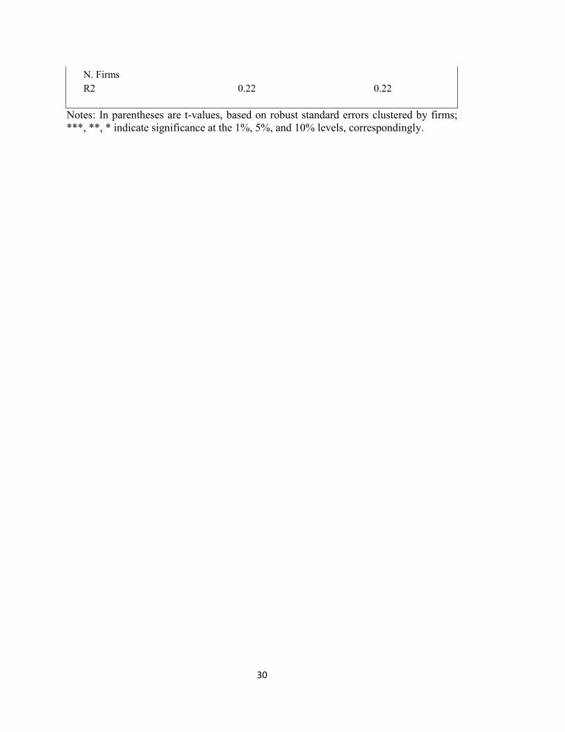
R2 0.22

0.22

Notes: In parentheses are t-values, based on robust standard errors clustered by firms;

***, **, * indicate significance at the 1%, 5%, and 10% levels, correspondingly.

31

Table 3. Single Equation Error Correction Model of Firm Profitability: Types of War

Systemic Effect

Sectoral Effect

Error Correction Rate

Profitabilityt-1 -0.25 *** (-58.93)

-0.25 *** (-58.92)

Short-Term Effect

∆Interstatet -0.01 *** (-3.91)

-0.01 *** (-3.92)

∆Interstatet * Defenset -

0.00

(0.22)

∆Intrastatet -0.01 *** (-5.24)

-0.01 *** (-5.25)

∆Intrastatet * Defenset -

0.00

(0.97)

∆Extrastatet -0.04 *** (-8.77)

-0.04 *** (-8.78)

∆Extrastatet * Defenset -

0.01 * (1.85)

∆Sizet 0.06 *** (68.49)

0.06 *** (68.48)

∆Leveraget 0.00

(-1.55)

0.00

(-1.55)

∆Dividendt -0.02 * (-1.72)

-0.02 * (-1.72)

∆Casht 0.00

(-0.30)

0.00

(-0.30)

∆Capitalt -0.09 *** (-11.85)

-0.09 *** (-11.86)

∆R&Dt 0.00 *** (-4.18)

0.00 *** (-4.19)

∆GDPt 0.00 *** (-4.61)

0.00 *** (-4.61)

∆GDPGrowtht 0.01 *** (6.42)

0.01 *** (6.42)

∆Inflationt 0.00 *** (4.44)

0.00 *** (4.45)

∆Opennnest -0.01 *** (-3.05)

-0.01 *** (-3.05)

∆ColdWart -0.02 *** (-3.20)

-0.02 *** (-3.20)

∆Democratt -0.01 *** (-5.34)

-0.01 *** (-5.35)

Long-Term Effect

Interstatet-1 0.00

(-1.59)

0.00

(-1.57)

Interstatet-1*Defenset -

-0.01 *** (-4.08)

Intrastatet-1 -0.01 *** (-3.33)

-0.01 *** (-3.34)

Intrastatet-1*Defenset -

0.01

(1.18)

Extrastatet-1 -0.01

(-1.18)

-0.01

(-1.18)

Extrastatet-1*Defenset -

0.00

(-0.48)

Sizet-1 0.00 *** (34.38)

0.00 *** (34.38)

Leveraget-1 0.00 *** (2.68)

0.00 *** (2.68)

Dividendt-1 0.00

(-0.96)

0.00

(-0.96)

Casht-1 -0.07 *** (-19.16)

-0.07 *** (-19.15)

Capitalt-1 -0.06 *** (-12.98)

-0.06 *** (-13.00)

R&Dt-1 0.00

(0.27)

0.00 *** (0.21)

GDPt-1 0.00 *** (2.60)

0.00 *** (2.59)

32

GDPGrowtht-1 0.01 *** (6.01)

0.01 *** (6.01)

Inflationt-1 0.00

(-1.56)

0.00

(-1.56)

Opennnest-1 -0.01 *** (-3.45)

-0.01 *** (-3.45)

ColdWart-1 -0.02 *** (-3.58)

-0.02 *** (-3.58)

Democratt-1 -0.01 *** (-3.88)

-0.01 *** (-3.88)

Defenset -

0.00

(-0.56)

Industry Fixed Effect Yes

Yes

Year Fixed Effect Yes

Yes

N. Obs. 144519

144519

N. Firms

R2 0.23

0.23

Notes: In parentheses are t-values, based on robust standard errors clustered by firms;

***, **, * indicate significance at the 1%, 5%, and 10% levels, correspondingly.

33

Table 4. Single Equation Error Correction Model of Firm Profitability: War

Characteristics

Systemic Effect

Sectoral Effect

Error Correction Rate

Profitabilityt-1 -0.247 *** (-58.89)

-0.24676 *** (-58.88)

Short-Term Effect

∆Durationt -2E-05 *** (-4.71)

-2.1E-05 *** (-4.64)

∆Durationt * Defenset -

-2.7E-05 *** (-2.97)

∆Severityt -8E-04 ** (-2.15)

-0.00079 ** (-2.14)

∆Severityt * Defenset -

-0.0007

(-1.08)

∆PProximityt -5E-07

(-1.40)

-4.6E-07

(-1.38)

∆PProximityt * Defenset -

2.83E-07

(0.48)

∆FProximityt 1E-04 *** (3.84)

0.000138 *** (3.77)

∆FProximityt * Defenset -

0.00015 ** (2.01)

∆Sizet 0.056

(68.53)

0.056 *** (68.52)

∆Leveraget -9E-05

(-1.53)

-8.8E-05

(-1.52)

∆Dividendt -0.015 * (-1.74)

-0.01547 * (-1.74)

∆Casht -0.001

(-0.28)

-0.00149

(-0.28)

∆Capitalt -0.089 *** (-11.83)

-0.08876 *** (-11.84)

∆R&Dt -1E-05 *** (-4.18)

-1.1E-05 *** (-4.19)

∆GDPt 2E-05

(0.53)

1.76E-05

(0.53)

∆GDPGrowtht 0.002

(1.00)

0.00175

(1.00)

∆Inflationt 0.002 ** (2.18)

0.001686 ** (2.18)

∆Opennnest 0.002

(1.23)

0.002437

(1.22)

∆ColdWart -7E-04

(-0.11)

-0.00072

(-0.12)

∆Democratt -0.006 * (-1.79)

-0.00633 * (-1.81)

Long-Term Effect

Durationt-1 -4E-05 *** (-4.54)

-4E-05 *** (-4.53)

Durationt-1*Defenset -

-4E-06

(-0.35)

Severityt-1 -0.002 *** (-3.38)

-0.00191 *** (-3.36)

Severityt-1*Defenset -

-0.00159 *** (-3.40)

PProximityt-1 -2E-07

(0.74)

-1.8E-07

(-0.31)

PProximityt-1*Defenset -

-8.3E-07

(-1.43)

FProximityt-1 5E-04 *** (7.43)

0.000449 *** (7.39)

FProximityt-1*Defenset -

0.000133

(1.43)

Sizet-1 0.005

(34.49)

0.00483 ***

Leveraget-1 1E-03 *** (2.67)

0.000983 *** (2.67)

Dividendt-1 -0.005

(-0.98)

-0.00473

(-0.98)

34

Casht-1 -0.067 *** (-19.14)

-0.06669 *** (-19.14)

Capitalt-1 -0.059 *** (-12.96)

-0.05887 *** (-12.97)

R&Dt-1 2E-07

(0.24)

1.7E-07

(0.18)

GDPt-1 3E-06

(0.47)

3.5E-06

(0.48)

GDPGrowtht-1 6E-04

(0.36)

0.000639

(0.37)

Inflationt-1 6E-04

(0.52)

0.000606

(0.51)

Opennnest-1 -0.004

(-1.53)

-0.00406

(-1.54)

ColdWart-1 -8E-04

(-0.11)

-0.00086

(-0.12)

Democratt-1 -0.01 *** (-2.71)

-0.01037 *** (-2.71)

Defencet

0.000604

(0.21)

Industry Fixed Effect Yes

Yes

Year Fixed Effect Yes

Yes

N. Obs 144519

144519

N. Firms

R2 0.22

0.22

Notes: In parentheses are t-values, based on robust standard errors clustered by firms;

***, **, * indicate significance at the 1%, 5%, and 10% levels, correspondingly.