wages, unions, and labour productivity: evidence from ... · wages, unions, and labour...

Wages, unions, and labour productivity:evidence from Indian cotton mills1

By BISHNUPRIYA GUPTA

Clark and Wolcott attribute the low productivity of Indian cotton textile workers totheir preference for low work effort, and suggest that unions resisted an increase inwork intensity. This article argues that low wages were due to surplus labour inagriculture. Low wages allowed the persistence of managerial inefficiencies andresulted in low productivity and work effort. It uses firm-level data from all the textileproducing regions in India to examine the relationship between unions and labourproductivity.The findings show that fewer workers were employed per machine in theunionized mills in Bombay and Ahmedabad, compared to the mills in less unionizedregions. These findings suggest that unionization increased wages and compelledmanagers to raise productivityehr_528 76..98

Why are there large differences in labour productivity across countries? Stan-dard economic theory emphasizes cross-country differences in capital

employed per worker. In a well-known paper, Clark compared labour productivityin cotton mills in different parts of the world in the early twentieth century andargued that although capital inputs were comparable, there were great differencesin labour productivity. Clark suggests that labour productivity differences deter-mined wage differentials across countries.2 Developed countries such as the USand Britain had high labour productivity, which resulted in high wages, while poorcountries such as India and Japan had low productivity and low wages. Clark goeson to argue that cultural factors may well explain the differences in work effort.3

Wolcott and Clark extend this argument to explain the divergent trajectory ofwages and productivity between Japan and India in the subsequent period.4 Theyclaim that Japanese workers increased their work effort over time and consequentlyearned higher wages. On the other hand, work norms in the Bombay cotton millindustry remained static.Wolcott and Clark argue that India’s lower efficiency wasdue to worker resistance to higher effort. Wolcott attributes worker resistance tounionization of cotton mill workers and lifelong employment contracts. Accordingto this view, a labour force of young female workers gave Japanese industry a

1 This article is dedicated to the memory of Raj Chandavarkar to whom I owe many discussions and theencouragement to revisit the history of cotton mills in India. I thank V. Bhaskar, Steve Broadberry, Greg Clark,Nick Crafts, Santhi Hejeebu, Morris D. Morris, Peter Lindert, JeffWilliamson, and GavinWright; the participantsof the Business History Conference in Lowell, the World Congress in Cliometrics in Venice, and seminars at theLondon School of Economics, and the Universities of Iowa, Davis, Warwick, York, Jerusalem, Boston, andSouthern Illinois for comments; and three anonymous referees for valuable suggestions. I am grateful to the staffat the Bombay Millowners’ Association and the Cotton Mills Federation in Bombay for giving me access to theirarchives and to the ESRC grant R.ECAA 0039 for financial support. The errors are mine alone.

2 Clark, ‘Why isn’t the whole world developed?’.3 See also Clark, Farewell to alms, pp. 353–65.4 Wolcott and Clark, ‘Why nations fail’.

Economic History Review, 64, S1 (2011), pp. 76–98

© Economic History Society 2010. Published by Blackwell Publishing, 9600 Garsington Road, Oxford OX4 2DQ, UK and 350 MainStreet, Malden, MA 02148, USA.

decisive advantage in pushing through organizational change that increased labourproductivity.5

This article takes a critical look at the arguments of Clark andWolcott and offersalternative explanations.While the observed correlation between wages and labourproductivity across countries is clear, the direction of causality is more difficult tounderstand. Did low wages in industry result from low effort, as Clark argues, ordid low wages lead to low effort? In this article it is argued that in India in the earlytwentieth century, the wage rate was determined in agriculture, which employedan overwhelming share of the workforce. In this labour surplus economy, wherethe marginal product of labour in agriculture was close to zero, the industrial wagewas low, as the Lewis model predicts.6 Low wages in the cotton mills created littleincentive for managers to bring about productivity-enhancing changes. Lowlabour productivity in cotton mills was a consequence of low wages.

A second question concerns the relation between worker militancy and labourproductivity. Did labour unions resist increases in productivity? This article uses anew data set of cotton mills from all regions in India. Unionization and workermilitancy differed greatly across the regions. This article also uses the regionalvariation in unionization to test whether the militant workers in the cotton mills inBombay were less productive, finding that regions with higher wages had higherlabour productivity. These were also regions where the workers were unionized.The presence of unions did not lead to lower productivity. On the contrary, byraising wages the unions contributed to raising labour productivity in the region.This reinforces the argument that the causality may go from wages to productivity.

The article is organized as follows: section I re-examines the arguments of Clarkand Wolcott. Section II presents a simple model of wage–effort trade-off. SectionIII discusses the organization of the industry and the factors that may explain highlabour use per machine. Section IV looks at the relationship between unionizationand wages. Section V presents an empirical analysis of firm-level data to quantifylabour use in different regions. The indicator of labour use employed here is thetotal number of workers employed daily. Section VI analyses the evidence forworkers’ preferences related to wage and effort, and the role of institutional factorsin determining the level of effort. Section VII concludes.

I

In 1910, British cotton mills used 3.8 plain looms per worker, New England mills8.0, Japanese mills 1.6, and Indian mills 1.9.7 While these differences can beexplained in terms of factor prices, it was not the case that capital productivity washigher in the poor countries. In the 1920s, if we normalize output per spindle-hourin Britain at 100, then output per spindle-hour in the US was 105, in Japan 115,and in India 99.8 Indian mills employed more workers per machine, but did nothave higher capital productivity. A spinner in Bombay attended 180–200 mulescompared to 500–600 in Britain. A weaver in Bombay operated two looms, while

5 Wolcott, ‘Perils of lifetime employment’, pp. 302–24.6 Lewis, ‘Economic development’, pp. 139–91.7 Clark, ‘Why isn’t the whole world developed?’.8 Ibid.

INDIAN COTTON MILLS 77

© Economic History Society 2010 Economic History Review, 64, S1 (2011)

a weaver in Britain was responsible for 4–5 looms.9 The work rate per hour ofIndian doffers was one-sixth that of their US counterparts and one-quarter that oftheir British counterparts.10 Other estimates put the productivity of labour inIndian mills at less than half of their British counterparts.11 Clark claims thatworker quality in terms of stature and education cannot explain differences inefficiency across countries. He attributes low labour productivity to a low level ofeffort that reflects preferences or cultural differences.12 Consequently, low produc-tivity is a determinant of low wages.

Clark sees low labour productivity as a determinant of low wages. However, thisview is inconsistent with a competitive labour market, where textile workers madeup only a small fraction of the total workforce. In India the entire industrialworkforce was less than 10 per cent of the total labour force, and cotton textileshad an even smaller share. Thus the wages of cotton textile workers were notdetermined by the level of labour productivity in cotton textiles, but mainly by thegeneral level of wages in the economy. If textile workers were substantially moreproductive, this would mainly be reflected in higher profits, with only a small effecton wages.

The Indian economy in the early twentieth century had all the characteristicsof a labour surplus economy, where the marginal product of labour in agriculturewas close to zero.The Lewis model of a dual economy suggests that surplus labourin the traditional sector keeps wages low in the modern sector. Over 75 per centof the workforce in India was employed in agriculture, producing just over50 per cent of the national output.13 A disaggregated picture of non-agriculturalemployment shows that only 10 per cent worked in industry, 1 per cent intransport, and just over 5 per cent in commerce.14 The rural–urban wage gap ledto migration.The wage rate in agriculture was close to subsistence level, due to thelow marginal product of labour. The urban wage was a mark-up on this outsideoption and was therefore constrained to remain close to that level as long as therewas surplus labour in agriculture. This is true not only of wages in the industrialsector, but also in other non-agricultural sectors, such as transport and trade.15

Wages in Indian agriculture stagnated over the next few decades.Yield per acrestagnated between 1890 and 1916 and declined thereafter until 1946.16 TheJapanese economy shows a different picture. Labour productivity in agriculturedoubled during the period 1885–1915, and the increase in agricultural outputaccounted for 40 per cent of the rise in national income, paving the way forindustrial growth.17 Rising productivity in agriculture increased wages. Therural–urban wage gap was small before 1910 and increased thereafter as the capital

9 Rutnagur, ‘Bombay industries’, p. 323.10 Clark, Farewell to alms, p. 359.11 Indian Textile Journal (hereafter ITJ), various issues.12 Clark, ‘Why isn’t the whole world developed?’.13 Sivasubramoniam, National income of India, pp. 33–4, 377.14 Ibid., pp. 33–4, 377.15 The low productivity of labour in other urban activities in India, such as the railways, as shown in Clark,

Farewell to alms, can also be explained in terms of low wages in a labour surplus economy, where the traditionalsector employs an overwhelming share of the workforce and the transport sector employs only 1%. So the wagein all sectors is determined by the wage in agriculture.

16 Blyn, Agricultural trends in India, pp. 316–17.17 Johnston, ‘Agricultural productivity’.

78 BISHNUPRIYA GUPTA


intensive sector paid higher wages.18 Output per worker in cotton textiles increasedby 180 per cent between 1907 and 1935.19

GDP per capita rose faster in Japan relative to India. In 1870, GDP per capitain Japan was just over 35 per cent more than that of India. By 1913 Japan had twicethe per capita income of India and by 1950 three times as much. Per capita GDPgrew by 0.54 per cent per annum in India during 1870–1913, about one-third ofJapan’s growth rate of 1.48 per cent per annum. The corresponding growth ratesin India and Japan during 1913–50 were -0.22 per cent and 0.89 per centrespectively.20 Money wages in Japanese cotton mills increased four times between1903–7 and 1918–22, while real wages doubled. In Indian cotton mills, moneywages doubled during the same period and real wages rose by less than 20 per cent(see table 1a). As wages increased in Japan, sectors producing tradable goods, suchas cotton textiles, were compelled to increase labour productivity to stay competi-tive. On the other hand, the Indian economy stagnated and wages did not risemuch until the First World War.The cotton mill entrepreneur faced little pressureto increase productivity.

Table 1b shows the trends in the relative cost of capital and labour in the twocountries. In India, the relative price of capital goods increased, whereas in Japan

18 C. Mosk, ‘Japan, industrialisation and economic growth’, EH.Net Encyclopaedia, R. Whaples, ed. (19 Jan.2004). URL http://eh.net/encyclopedia/article/mosk.japan.final.

19 Clark, Farewell to alms, p. 347.20 Maddison, World economy, pp. 264–5; Sivasubramoniam, National income of India, p. 33.

Table 1. (a) Changes in real wages: Japan and India (b) Changes in wages and costof capital: Japan and India

(a) Changes in real wages: Japan and India

Japan India

1903–7 100 1001908–12 116 1081913–17 116 1021918–22 181 1191923–7 239 1601928–32 295 205

(b) Changes in wages and cost of capital: Japan and India

Years

Japan India

Capital goodsprice index

Money wageindex for

cotton spinners

Relativeprice of

capital–labour

Textilemachineryprice index

Money wageindex in

cotton mills

Relativeprice of

capital–labour

1903–7 100.0 100.0 1.00 100.0 100.0 1.001908–12 103.7 125.6 0.83 106.2 112.5 0.941913–17 131.8 148.8 0.89 196.3 130.7 1.501918–22 258.74 429.8 0.60 336.6 219.5 1.531923–7 232.0 525.1 0.44 242.1 252.3 0.941928–32 174.8 465.1 0.38 204.9 265.19 0.77

Sources: Real wage indices have been calculated from Otsuka, Ranis, and Saxonhouse, Comparative technology-choice, tab. 5.1,p. 68 (for Japan), and Bagchi, Private investment, p. 122 (for India).



the relative price of capital goods declined continuously, creating the momentumfor technological change. An Indian worker produced 0.75 pounds of yarn perhour in 1890–4, and this remained static at 0.73 in 1915–19. In Japan, yarn perworker more than doubled, from 0.80 to 1.91 in the same years.21 As culturalpreferences are slow to change, it is difficult to explain the dramatic change inJapan in terms of sudden changes in effort leading to a rise in wages.22 Wage-drivenproductivity growth is a more plausible explanation.

Wright discusses the identification problem in the context of the relationshipbetween wages and labour productivity. He argues that if exogenous shocks lead torise in real wages, then wage increases must be the cause of productivity increases.This was true in the 1920s in the US when prices fell and flows of immigrationdeclined and therefore productivity growth was the response of employers tohigher labour costs.23 Huberman argues that cotton mills in Lancashire in themid-nineteenth century standardized piece rates and forced the inefficient firms toraise productivity with a given technology. If firms had lower wages, workers wouldreduce their effort and lower their output.24 In the Indian context, the First WorldWar constituted such an exogenous shock to wages. As imports were cut off, localproduction filled the gap and the rising demand for labour increased wages.

There are two possible scenarios. First, if cultural preferences determine loweffort and low wages, then exogenous shocks to wages will not raise labourproductivity. On the other hand, if it reflects inefficiency rather than workers’preferences, then an exogenous shock that increases wages will cause a rise inlabour productivity. In the second case, it can be argued that wages determineproductivity. In order to understand why firms operated at a sub-optimal level andwhat prompted them to become more efficient, the next section sets out a simplemodel of the wage–effort trade-off.

II

Let e denote effort, and let us measure effort so that one unit of effort results in oneunit of output. Let p denote the price of output, k the capital requirement perworker, and r the interest rate. Let w denote the wage per unit of effort, so that theprofits of the firm per worker can be written as

π = − −ep w rk (1)

Turning to the representative worker, let us assume that the utility of the worker,U (w, e), increases with wage, but decreases with effort. Figure 1a shows the typicalindifference curve of the worker IC, corresponding to a given utility level. Let usnow consider what effort choice would be a Pareto efficient arrangement, given thepreferences of the worker and the production technology.To do this, we can graphthe iso-profit curves of the firm. These are straight lines with slope p. An efficientarrangement corresponds to a point of tangency between the worker’s indifferencecurve and the iso-profit curve IP. Thus e* is the efficient choice of effort in thiscontext.

21 Wolcott and Clark, ‘Why nations fail’.22 Mass and Lazonick, ‘British cotton industry’.23 Wright, ‘Productivity growth’.24 Huberman, ‘Piece rates reconsidered’.



There can be many Pareto efficient arrangements, with different distribution ofthe gains between the firm and the worker. Now suppose that the bargainingpower of workers increases, due to unionization. With efficient bargaining, thisimplies a move to a new efficient point, e**, on a higher worker indifferencecurve. If income and leisure are both normal goods, as we would expect, then wewill have higher wages and lower effort, so that e** < e*. Thus if the initialoutcome and final outcomes are both efficient, unionization will be accompaniedby a fall in productivity.

Let us now consider the case where existing effort arrangements are inefficientlylow, and are at a level e’ that is less than e*.This is indicated in figure 1b. Since thisis Pareto inefficient, there is a way to make both the worker and the firm better off.This involves an increase in worker effort towards e*, where the worker is com-pensated for this by an increase in wage. Here unionization can lead to a moreefficient outcome.

Wolcott and Clark argue that low effort reflected workers’ preferences, so thatarrangements were Pareto efficient.25 In terms of the analysis presented here,actual effort–wage choices were in fact close to the point e*, so that it did not makeeconomic sense to increase effort. Clark argues that the failure to raise effort levelsin a cotton mill in Madras where automatic looms were introduced is suggestive ofworker preference for low effort.26 According to this view, unions therefore have adetrimental effect on labour productivity.

The second scenario is that actual arrangements were Pareto inefficient; e’ is wellbelow e*. so that both workers and firms could be made better off by wage–productivity agreements, where the worker agreed to raise work effort in exchangefor higher wages. For this explanation to hold, there must be a reason why the twoparties failed to make a Pareto-improving trade. This could be a failure of initia-tive, possibly based on a lack of information. For two parties to make such animprovement, one of them must recognize the potential for mutual gain, and hasto initiate the improvement. The specific institutional structure of management

25 Clark, ‘Why isn’t the whole world developed?’; Wolcott and Clark, ‘Why nations fail’.26 Clark, Farewell to alms, pp. 362–5.

IC(a)

ee**

wIP

e*

(b)

ee*

w

e′

IP

Figure 1. (a, b)Wage–effort trade off



may have created inefficiencies in the system. Unions in this context may play animportant role in moving to a more efficient arrangement.

Consider an exogenous shock, such as the FirstWorldWar.Wages rose due to thedemand shock, but when demand fell, as it did after the war, the unions resistedwage cuts. The only way the firms could stay profitable was to raise labourproductivity. Therefore unionized firms with higher wages could achieve higherlabour efficiency. In order to understand whether this indeed was the case inBombay cotton mills, the econometric analysis in this article compares firms inBombay city (hereafter Bombay) with firms in less unionized regions in section V.Sections III and IV discuss the organization and institutional structure of cottonmills in India.

III

The cotton textile industry was mainly an import-substituting activity, competingwith imports from Lancashire. The first cotton mills were set up in Bombay.Initially the main output was yarn for the domestic handloom industry and forexport to the Chinese market. Over time, spinning mills bought their own loomsand began producing cloth.While Bombay concentrated on producing low-qualityyarn, Ahmedabad specialized in higher-quality yarn and cloth and competed withimports from Britain. During the war, the substitution of imports gained momen-tum and the trend continued after the war. One problem faced by the industry wasthat each firm produced a variety of output and therefore could not get the benefitsfrom specialization.

However, costs were low as labour was cheap and the raw material was availablelocally. The industry had a special management structure, whereby a managingagent raised capital and managed the financial side of the business. Production wasleft in the hands of technical supervisors and labour supervisors, known as jobbers.The agents mostly came from the merchant class and had little technical training.The majority of the agency directors were Indians, who had made money in thecotton and opium trade and moved into industry as profits in trade began todecline.27 Table 2 shows the background of the directors and of technical staff inBombay.The managing agents relied initially on the men from Lancashire for thetechnical side of production. Over the years, Indian technicians filled this impor-

27 Vicziany, ‘Cotton trade’.

Table 2. Social origins of managers in Bombay cotton mills

Technical personnel Directors 1925

1895 1925 MerchantsTechnical

background Lawyers

Parsi 112 201 30 9 10Hindu 21 67 74 0 3Muslim 5 6 19 0 0Jewish 3 11 6 0 0European 104 113 20 2 2

Source: Rutnagur, ‘Bombay industries’, pp. 251–3.



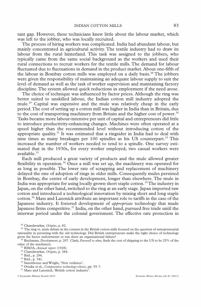
tant gap. However, these technicians knew little about the labour market, whichwas left to the jobber, who was locally recruited.

The process of hiring workers was complicated. India had abundant labour, butmainly concentrated in agricultural activity. The textile industry had to draw itslabour from the rural hinterland. This task was assigned to the jobbers, whotypically came from the same social background as the workers and used theirrural connections to recruit workers for the textile mills. The demand for labourfluctuated due to fluctuations in demand in the product market. About one-fifth ofthe labour in Bombay cotton mills was employed on a daily basis.28 The jobberswere given the responsibility of maintaining an adequate labour supply to suit thelevel of demand as well as the task of worker supervision and maintaining factorydiscipline. The system allowed quick reductions in employment if the need arose.

The choice of technique was influenced by factor prices. Although the ring wasbetter suited to unskilled labour, the Indian cotton mill industry adopted themule.29 Capital was expensive and the mule was relatively cheap in the earlyperiod.The cost of setting up a cotton mill was higher in India than in Britain, dueto the cost of transporting machinery from Britain and the higher cost of power.30

Tasks became more labour-intensive per unit of capital and entrepreneurs did littleto introduce productivity-enhancing changes. Machines were often operated at aspeed higher than the recommended level without introducing cotton of theappropriate quality.31 It was estimated that a ringsider in India had to deal withnine times as many breakages per 100 spindles as his US counterpart.33 Thisincreased the number of workers needed to tend to a spindle. One survey esti-mated that in the 1930s, for every worker employed, two casual workers wereavailable.33

Each mill produced a great variety of products and the mule allowed greaterflexibility in operation.34 Once a mill was set up, the machinery was operated foras long as possible. The lower rate of scrapping and replacement of machinerydelayed the rate of adoption of rings in older mills. Consequently mules persistedin Bombay, the centre of early development, longer than elsewhere. The mule inIndia was appropriate for using locally grown short staple cotton.35 The industry inJapan, on the other hand, switched to the ring at an early stage. Japan imported rawcotton and introduced a technological innovation by mixing short and long staplecotton.36 Mass and Lazonick attribute an important role to tariffs in the case of theJapanese industry. It fostered development of appropriate technology that madeJapanese firms competitive.37 India, on the other hand, pursued free trade until theinterwar period under the colonial government. The effective rate protection in

28 Chandavarkar, Origins, p. 82.29 The ring vs. mule debate in the context in the British cotton mills focused on the question of entrepreneurial

rationality in persisting with the old technology. Did British entrepreneurs make the right choice of technologygiven the factor endowments or was there an organizational failure?

30 Buchanan, Development, p. 207. Clark, Farewell to alms, finds the cost of shipping to the US to be 25% of thevalue of the machinery.

31 BMOA, Annual report (1928).32 Chandavarkar, Origins, p. 284.33 Ibid., p. 296.34 Ibid., p. 341.35 Saxonhouse and Wright, ‘New evidence’.36 Otsuka et al., Comparative technology-choice, pp. 55–7.37 Mass and Lazonick, ‘British cotton industry’.



spinning in Japan on the eve of the First World War was 120 per cent and in Indiazero.38An alternative view has emphasized the lack of technical knowledge of themanaging agents and the presence of British technical personnel as the cause ofIndia’s failure to switch to ring spinning.39 Mixing of cotton was not adopted inIndia due to the lack of incentives and also due to the managers’ lack of technicalknowledge.40 The Tariff Board in 1927 saw high labour use per machine as anorganizational problem:

We cannot too strongly emphasise that no increase in outturn per operative can bereasonably expected unless they are provided with proper raw material. Thereundoubtedly exists a tendency in India to spin higher counts of yarn from cotton thanthe quality of cotton warrants. This reduces production, is injurious to quality andincreases the work of the operative in both spinning and weaving by the large numberof breakages.41

IV

In the first decades of the twentieth century, labour in the cotton mills was stillunorganized. Resistance to low wages and working conditions was sporadic andlacked centralized organization. Industrial action in Bombay and Ahmedabad wasmainly against wage cuts. Spontaneous protests by textile workers in Bombay hadbeen a part of the industry from its beginning. The early protests started in onemill and spread to others.The wave of strikes in 1900–1 came in response to wagecuts in 20 mills, resulting in 20,000 workers going on strike for 10 days.42 By themid-1920s these protests were coordinated by the trade unions.

Wages rose during the war in response to increased demand.While money wagesin Bombay, Ahmedabad, and Calcutta43 had been comparable before 1914, wagesrose sharply in Bombay and Ahmedabad thereafter (see figure 2). The averagewage in Bombay was 20 per cent higher than the average wage in Ahmedabad onthe eve of the First World War. During the war, cotton mills paid a war bonus of10 per cent from 1917 to be followed by a ‘dear food allowance’ of 15 per centfrom 1918.44 Between 1914 and 1921, wages rose by 87 per cent in Bombay andby 122 per cent in Ahmedabad.45 Table 3 shows a comparison of wages in the twocities and the rest of Bombay Presidency in 1929. Clearly the difference in wagesbetween Bombay and Ahmedabad was marginal, but these amounts were higherthan those paid to workers in other textile producing regions.

When demand conditions changed at the end of the war, the response of themajority of firms was to reduce wages. It was when firms tried to cut wages thatresistance erupted on the shop floor. As early as 1900, a commentator wrote: ‘The

38 Otsuka et al., Comparative technology-choice, p. 70.39 Kiyokawa, ‘Technical adaptations’.40 Ibid.41 BMOA, Annual report (1928).42 Morris, Emergence, pp. 178–9.43 Calcutta was the other major industrial centre, although the main industry there was jute rather than cotton.44 Kooiman, Bombay textile labour, pp. 51–2.45 Bombay Labour Office, Report on enquiry (1923).



principal reason why people go on strike is that of wage reduction. In the cottonmill industry, mill agents have thought that the reduction in wages is the firstremedy against hard times’.46

The first strike action that affected the entire industry in Bombay occurred inDecember of 1918 and involved 125,000 workers.47 In 1919, 150,000 workerswent on strike for 12 days, followed by a general strike in 1920 that lasted for amonth.48 The disputes continued into the 1920s in response to cuts in wartimepayments. By this stage, trade unions had established a strong presence in theindustry. A strike in 1925 lasted several weeks. As several cotton mills in Bombaysought to introduce a higher workload, the trade unions organized industrialaction in 1928 that lasted over six months. The year 1929 saw further industrialaction by the communist-led union, but this was opposed by the moderates anddid not have the same effect as the strike in the previous year.49

46 ITJ (Feb. 1900).47 Buchanan, Development, p. 427.48 Bombay Labour Office, Report on enquiry (1926).49 Morris, Emergence, pp. 181–4.

0.00

5.00

10.00

15.00

20.00

25.00

30.00

35.00

40.00

1900

1903

1906

1909

1912

1915

1918

1921

1924

1927

1930

1933

1936

1939

Years

Wag

es

Bombay

Ahmedabad

Jute in Calcutta

Figure 2. Money wage in the cotton textiles industry

Table 3. Wage differential in Bombay Presidency,1929 (daily average earning in rupees)

Bombay Ahmedabad Sholapur Baroda Others

Men 1.45 1.39 1.00 1.03 1.00Women 0.78 0.80 0.40 0.57 0.54All workers 1.26 1.24 0.80 0.95 0.87

Source: Pearse, Cotton industry, p. 109.



Worker resistance to a reduction in wages was not specific to Bombay.Wage cutsin the cotton textile industry in the southern US in the 1920s had led to resistanceeven among non-unionized workers.50 Wright argues that once wages have risendue to an exogenous shock, rational employers are willing to take that wage rate asgiven and increase the productivity of capital and labour.51 Domenech’s work onthe non-unionized Catalan cotton textile industry in the late nineteenth centuryfinds that workers resisted wage cuts, as in more unionized countries, and firmsadjusted by reducing output and hours of work in the downturn.52 In the Bombaycotton mills in the interwar years, attempts at wage cuts led to industrial action. Onthe other hand, reducing total employment proved easier due to the large numberof casual workers employed on a daily basis. Aggregate employment declined in thecotton mills in Bombay from the late 1920s.

There were protests against cuts in wages in Ahmedabad too. With Gandhi’sinvolvement, workers in Ahmedabad sought consensual solutions through indus-trial arbitration. This period coincided with economic nationalism in the anti-imperialist struggle. The principle of arbitration was helped by shared interestsbetween the workers and the capitalists in the boycott of foreign goods.53 However,sporadic industrial action continued in the early 1920s and not all firms supportedthe principle of arbitration. In 1923 the industry implemented a wage cut of 15 percent and for the rest of the decade industrial arbitration dealt with issues such ashealth, education, and housing rather than wages.54 In comparison to Bombay,industrial relations in Ahmedabad remained more peaceful.

In Bombay cotton mills, 42.5 per cent of the workers were in trade unions,compared to 29 per cent in Ahmedabad, and only 5 per cent in Sholapur.55 Textileworkers in Delhi did not have a union, and the union in Madras had a relativelylow-key presence.56 The jute labour union in Calcutta, the other major industrialregion, did not succeed in involving the workers in a strike in 1929 and representedonly 4 per cent of the workforce.

There is no information on the number of strikes and workers involved in textilemills for the whole of India. However, there is a lot of qualitative evidence thatshows that Bombay was the centre of industrial action in the cotton textileindustry. Table 4 shows the incidence of all industrial disputes across differentregions of the Bombay Presidency, where the majority of the textile firms werelocated. Of the 401 strikes in Bombay accounting for 91 per cent of the workingdays lost, an overwhelming 79 per cent were in textile mills.57 Rough calculationsshow that the number of working days lost account for 12–13 per cent of the totalin Bombay.58

The effect of unionization on labour productivity has been debated in thecontext of industrialized economies. Freeman and Medoff argue that unions can

50 Wright, ‘Cheap labour’.51 Ibid.52 Domenech, ‘Labour market adjustment’.53 Patel, Making of industrial relations, pp. 54–6.54 Ibid., pp. 64, 81–4.55 Bagchi, Private investment, p. 140.56 Ibid.57 Pearse, Cotton industry, p. 95.58 The calculations have been based on a nine-year period, 1921–9, and therefore do not correspond exactly to

the period covered by tab. 4.The total workers in Bombay have been multiplied by 50 or 52 weeks and have beenassumed to work six days a week.



increase labour productivity by reducing labour turnover and improving manage-rial practices.59 The presence of unions can increase productivity by makingmanagers keen to reduce organizational slack.60 The empirical evidence is mixed.Research using data from US industries shows that unions had a positive effect onlabour productivity.61 The UK evidence is less clear-cut. Recent work suggests thatmulti-unionism has had a negative effect on productivity in the UK, while inGermany cooperative practice through work councils has had a positive effect onproductivity.62

How did the presence of unions in Bombay and Ahmedabad affect labourproductivity? Wolcott and Clark argue that in the 1920s, when cotton mills wereunder pressure to increase productivity, worker militancy in Bombay cotton millsprevented organizational change.63 Wolcott and Clark’s analysis does not allowinter-regional comparison. Consequently, their estimation does not identifywhether worker resistance prevented increases in labour productivity relative toother regions in India. With the new data set of cotton mills from all regions inIndia, it is possible to compare Bombay to the rest of India and test empiricallywhether Bombay mills had lower labour productivity. This makes it possible toidentify the effect of workers’ militancy on labour productivity in a particularregion.64 The empirical analysis is presented in the next section.

V

One way to analyse the role of unions is to compare labour productivity acrossdifferent regions in India. In the absence of firm-level output data, the measure of

59 Freeman and Medoff, What do unions do?, pp. 162–80.60 Metcalf, ‘Unions and productivity’.61 Brown and Medoff, ‘Trade unions’; Allen, ‘Unionisation’; Clark, ‘Unionisation’.62 Metcalf, ‘Unions and productivity’.63 Wolcott and Clark, ‘Why nations fail’.64 There is some information, although not systematic, on strikes in different cities.This again is at the level of

the region and not the firm, and therefore a regional dummy is a good measure.

Table 4. Industrial disputes in Bombay presidency: April 1921–June 1929

No of disputes No. of workers involved No. of working days lost

Bombay 401 1,077,927 49,297,817Ahmedabad 221 135,200 2,605,087Sholapur 10 39,484 1,214,434Viramgam 8 3,705 32,854Broach 22 8,966 85,022Karachi 14 9,893 395,554Jalgaon 7 4,445 56,990Surat 12 4,840 35,254Poona 11 3,763 40,903Rest 32 21,228 181,399Bombay presidency 738 1,309,511 53,949,314Share of textile mills 612 1,233,170 52,450,814Bombay n.a. n.a. 48,259,737Ahmedabad n.a. n.a. 2,604,737Sholapur n.a. n.a. 1,214,434

Source: Pearse, Cotton industry, p. 95; Bagchi, Private investment, p. 143.



labour productivity used here, as in Wolcott and Clark, is labour use per machine,defined as the number of workers per machine.65 This captures total factor pro-ductivity if machines are the same across cotton mills in all regions.66 Given thatmachines were similar and sold by a handful of machinery producers, this is not abad measure.

If organized labour resistance was important in influencing work norms,Bombay should have had a higher use of labour per machine compared to otherregions. On the other hand, if union activity mainly prevented wage cuts and/orhigher wages forced employers to initiate productivity increases, one should findthat Bombay had higher labour productivity and fewer workers per machine.Secondly, Bombay and Ahmedabad, with similar levels of wages in the 1920s,should show similar levels of labour use. A comparison with Ahmedabad is also ofinterest as the two regions had different experiences of labour resistance. Didcooperation rather than conflict lead to efficiency gains in Ahmedabad? If labourresistance explains inefficiency then Bombay should have employed more workersper machine relative to Ahmedabad.

Wolcott and Clark used firm-level data from Bombay from the annual reports ofthe Bombay Millowners’ Association (hereafter BMOA). The statistical appendixof the BMOA reports includes firm-level information from other regions in India,which have been put together here with the original data used by Wolcott andClark.This is the first time such a data set has been analysed.The data used hereare at the level of the firm and provide information on the number of workersemployed daily in each firm and the machinery used. The latter is available bycategory (that is, mules, rings, and looms).The data are for the years 1889, 1910,1917, 1929, and 1933. Firm-level information for 1889 is being used here for thefirst time, and allows us to go back to the period when worker resistance had yetto make an impact on the industry. It is helpful to consider the year 1910, as it isbefore the war and is also the year used in Clark’s international comparison.67 Theyear 1917 reflects a situation of increased output in the industry as a result of thewar.The years 1929 and 1933 are of particular interest as these follow a decade oflabour strife.

Table 5 shows the use of capital and labour in cotton mills in different regions.Here the focus is on Bombay relative to Ahmedabad and the rest of India. Bombayhad the highest concentration of cotton mills in 1889, while Ahmedabad was stillmarginal. By 1910 both cities had roughly the same number of mills. Ahmedabadhad a large share of rings as newer mills were more likely to adopt the ring, whileolder mills in Bombay with an existing capacity of mules were slow in switching torings. Ahmedabad also had more looms. The average size of mills in Bombay waslarger. By 1917 the changes in Bombay were noticeable. The switch to rings andlooms was well underway.There was also an increase in the average size of the mill.Several mills went out of business by 1929 and more disappeared by 1933. ForAhmedabad, on other the other hand, there is evidence of an increase in size aswell as new mills being set up.

65 Wolcott and Clark, ‘Why nations fail’, pp. 397–423.66 Firms all over India imported their equipment from a few British firms. Clark, ‘Why isn’t the whole world

developed?’, also finds this to be the case at the international level in 1910.67 Clark: ‘Why isn’t the whole world developed?’.



In the absence of information on union membership at the level of the firm, theregional difference in labour movement is used here in order to understand itseffect on labour productivity in different regions. Bombay and Ahmedabad wereregions with union activity, while the other regions were not.The hypothesis testedis as follows: Bombay is significantly different from the rest of India in terms of themeasure of labour productivity outlined above.

The dependent variable, the number of workers employed daily, is regressed onthe number of mules, rings, and looms within a firm. To allow for the possibilitythat labour in a particular region, Bombay or Ahmedabad, is systematically less (ormore) efficient, a dummy variable for the region is interacted with each of themachinery variables. That is, our regression takes the form:

Nit

l

= +( ) + +( )+ +

+ +

+

β γ μ β γ μβ γ μ

m i i it r i i it

i

BD AD Mule BD AD RingBD

1 11 AAD Loomi it it( ) + ε (2)

where Nit is employment in firm i in year t, Muleit is the number of mules used bythe firm in this year, and so on, and BDi is a dummy variable that takes the value1 if the firm is in Bombay and ADi is a dummy variable that takes the value 1 if thefirm is in Ahmedabad.This equation is estimated separately for each year; that is,

Table 5. Average capital and labour use in cottonmills

Bombay Ahmedabad Rest of India

1889Spindles 29,725 22,423 26,005Looms 252 212 20Workersa 996 779 884No. of firms 53 7 441910Mules 11,133 1,494 7,888Rings 23,720 18,648 20,453Loom 296 305 291Workersa 955 833 1,101No. of firms 79 72 571917Mules 7,591 781 5,280Rings 29,433 20,236 22,873Loom 724 391 480Workersa 1,562 817 1,175No. of firms 77 82 721929Mules 4,637 494 2,940Rings 39,812 21,007 26,670Loom 994 464 584Workersa 1,423 968 1,213No. of firms 75 111 1001933Mules 3,636 177 2,200Rings 41,930 24,071 28,642Loom 1,014 526 608Workersa 1,863 1,041 1,367No. of firms 67 128 103

Note: a No. of workers employed daily.Source: BMOA, Annual reports (various years), apps.



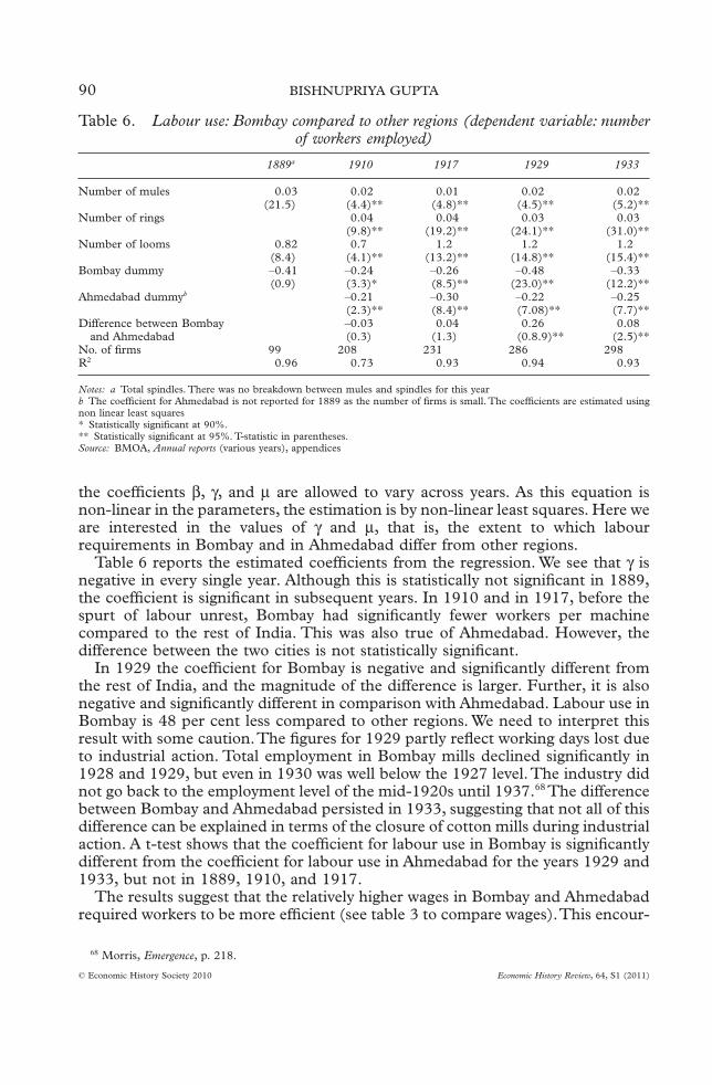
the coefficients b, g, and m are allowed to vary across years. As this equation isnon-linear in the parameters, the estimation is by non-linear least squares. Here weare interested in the values of g and m, that is, the extent to which labourrequirements in Bombay and in Ahmedabad differ from other regions.

Table 6 reports the estimated coefficients from the regression. We see that g isnegative in every single year. Although this is statistically not significant in 1889,the coefficient is significant in subsequent years. In 1910 and in 1917, before thespurt of labour unrest, Bombay had significantly fewer workers per machinecompared to the rest of India. This was also true of Ahmedabad. However, thedifference between the two cities is not statistically significant.

In 1929 the coefficient for Bombay is negative and significantly different fromthe rest of India, and the magnitude of the difference is larger. Further, it is alsonegative and significantly different in comparison with Ahmedabad. Labour use inBombay is 48 per cent less compared to other regions. We need to interpret thisresult with some caution.The figures for 1929 partly reflect working days lost dueto industrial action. Total employment in Bombay mills declined significantly in1928 and 1929, but even in 1930 was well below the 1927 level.The industry didnot go back to the employment level of the mid-1920s until 1937.68 The differencebetween Bombay and Ahmedabad persisted in 1933, suggesting that not all of thisdifference can be explained in terms of the closure of cotton mills during industrialaction. A t-test shows that the coefficient for labour use in Bombay is significantlydifferent from the coefficient for labour use in Ahmedabad for the years 1929 and1933, but not in 1889, 1910, and 1917.

The results suggest that the relatively higher wages in Bombay and Ahmedabadrequired workers to be more efficient (see table 3 to compare wages).This encour-

68 Morris, Emergence, p. 218.

Table 6. Labour use: Bombay compared to other regions (dependent variable: numberof workers employed)

1889a 1910 1917 1929 1933

Number of mules 0.03 0.02 0.01 0.02 0.02(21.5) (4.4)** (4.8)** (4.5)** (5.2)**

Number of rings 0.04 0.04 0.03 0.03(9.8)** (19.2)** (24.1)** (31.0)**

Number of looms 0.82 0.7 1.2 1.2 1.2(8.4) (4.1)** (13.2)** (14.8)** (15.4)**

Bombay dummy –0.41 –0.24 –0.26 –0.48 –0.33(0.9) (3.3)* (8.5)** (23.0)** (12.2)**

Ahmedabad dummyb –0.21 –0.30 –0.22 –0.25(2.3)** (8.4)** (7.08)** (7.7)**

Difference between Bombayand Ahmedabad

–0.03 0.04 0.26 0.08(0.3) (1.3) (0.8.9)** (2.5)**

No. of firms 99 208 231 286 298R2 0.96 0.73 0.93 0.94 0.93

Notes: a Total spindles. There was no breakdown between mules and spindles for this yearb The coefficient for Ahmedabad is not reported for 1889 as the number of firms is small. The coefficients are estimated usingnon linear least squares* Statistically significant at 90%.** Statistically significant at 95%. T-statistic in parentheses.Source: BMOA, Annual reports (various years), appendices



aged firms to economize on wage costs in order to remain competitive in theproduct market. Although the wage difference between Bombay and Ahmedabadwas marginal after 1929, there was a significant difference in labour productivity.This is puzzling. However, a closer examination suggests that the product andfactor markets in the two cities were very different. Firms in Ahmedabad producedfiner-quality yarn and cloth and competed with British imports. Bombay, on theother hand, produced more lower-count yarn and exported to the Chinese market.This export market in yarn disappeared after the war. Simple calculations of theprofits of the firms in the two cities show that profits fell faster in Bombay.69

Consequently, the pressure on entrepreneurs in Bombay to reduce inefficiency wasgreater.

The point estimate on Bombay shows a reduction in labour use between 1910and 1933. The standard error in 1910 is large, but relatively smaller in 1933, andsuggests that the mills were more similar in labour use in 1933 compared to 1910.In other words, less efficient mills reduced labour use per machine or went out ofbusiness.

Bombay mills had a high turnover of the workforce and a large proportion werecasual workers, estimated to constitute about 28 per cent of the workforce.70 Thismade it relatively easier to reduce employment. Estimates based on the data setpresented here show that Bombay saved in total wage costs as the number ofworkers per machine declined.Wage cost per unit of output in Bombay was 3 percent lower in 1933 relative to the rest of India, while in Ahmedabad it was roughly4 per cent higher (see table 7). These figures suggest that efficiency gains weremade by Bombay mills in the 1920s. Falling profits, older machinery, and changesin the product market created additional pressure on firms in Bombay to bringabout organizational change. There is no evidence that unionization prevented arise in productivity. On the contrary, firms in Bombay were more productive.

VI

Having ruled out the negative effect of unions on labour productivity, let us nowgo back to the model of wage–effort trade-off. Did workers show a preference forlow effort? Evidence on indebtedness suggests that the majority of the workersearned well below their expenditure levels. A survey conducted by the BombayLabour Office showed that in 1926, 47 per cent of families and 45 per cent of

69 Patel, Making of industrial relations, p. 34.70 Chandavarkar, Origins, p. 296.

Table 7. Wage cost per unit of output

Rest of India Bombay Ahmedabad

1929 1.00 0.75* 1.081933 1.00 0.97 1.04

Source: Tabs. 3 and 6.Note: The index is calculated using wages for men in 1929 and labour produc-tivity coefficients for respective years.* The low value here reflects the number of days lost in strike action.



single men were in debt.71 This on average was equal to two-and-a-half months’earnings at an average interest of 75 per cent per year. In Ahmedabad 69 per centof families were in debt, while in Sholapur the figure was 63 per cent.72 Most of theworkers sent money to families in the villages. Many incurred debts due tomarriage and other social customs. Whatever the cause, the debt burden wouldhave made higher earnings attractive to most cotton mill workers. It is unlikelythat, given the right incentive, the worker would not have been willing to offergreater effort.

Indirect evidence also suggests that the workers were prepared to increase effortin return for higher wages. The industry in Bombay had a wide differential inwages across firms for the same category of workers. This was noted as early as1893. The differential increased over time, suggesting that greater effort wasrewarded by higher pay. The maximum difference before 1920 was about 30 percent between high and low wages. This figure rose 33 per cent for one-side ringspinners, 34 per cent for two-loom weavers, 87 per cent for grey winders, and73 per cent for reelers in 1926. The corresponding figures were even higher in1933: 46 per cent, 90 per cent, 63 per cent, and 175 per cent respectively.73 Theweavers, winders, and reelers were on piece rates and the widening pay differencesreflect differences in effort.74 The differential in pay among both piece and timeworkers was significant even within the same district.75

The efficient mills attracted better workers by offering them higher wages.Workers tended to compete for jobs in mills that had better pay and better workingconditions. In mills that had poor-quality machines, jobbers had to attract workersby lending them money or standing as a guarantor for loans.76 Newer mills tried toreduce the cost of training by luring away efficient workers from existing employ-ment.77 Competition for more efficient workers raised wages. Mills such asSassoon, Bombay Dyeing, Finlay, and Kohinoor were ready to pay more for highereffort.78

There are many examples of workers accepting greater workloads whenrewarded by higher pay. In general, piece-rate workers earned more than time-rateworkers. This suggests that workers did respond to incentives towards higherearnings (see table 8). Four-loom weavers earned 50 per cent more than two-loomweavers (see table 9). Workers who were willing to undertake greater workloadswere favoured when chances of promotion appeared.79 Jobs were highly differen-tiated in the context of a labour-intensive technology. Yet when two jobs werecombined, as in Tata’s Swadeshi mills, the worker was paid more, suggesting anefficiency–wage trade-off.80 Absenteeism was lower among piece-rate male workersin Bombay, particularly among weavers.81 There is little evidence to suggest thatthe inefficient equilibrium was determined by workers’ preferences.

71 Pearse, Cotton industry, pp. 92–3.72 Ibid.73 Bombay Labour Office, Report on enquiry (1921, 1926); Bombay Labour Office, Wages and unemployment.74 Morris, Emergence, pp. 157–8.75 Ibid., p. 160.76 Chandavarkar, Origins, pp. 301–2.77 Morris, Emergence, p. 161.78 Chandavarkar, Origins, p. 351.79 Ibid., p. 323.80 Ibid., p. 317.81 Bombay Labour Office, Report on enquiry (1923), p. 8.



Was the low wage–low effort equilibrium caused by an institutional failure? Halland Jones show that institutional differences explain differences in labour produc-tivity across countries.82 In the Indian context, it may be argued that the mana-gerial structure in cotton mills created certain inefficiencies. The three tiers ofmanagement created self-contained spheres of function and resulted in informa-tion gaps. Madholkar documents the friction between the men from Lancashireand the managing agents, and sees the presence of the jobber as the crucial factorin reducing the managing agent’s reliance on the technicians.The agents’ distrustof the technicians removed them from the sphere of decision making. The agentmade decisions regarding the purchase of inputs and the technicians were asked toproduce a certain output per machine.83An additional reason might have been theincentives of the managing agents, who held overall responsibility for the organi-zation. Right up to the turn of the twentieth century, the managing agents’ returnsdepended upon the output of the firm rather than profits, and provided relativelyweak incentives to engage in cost reductions. Even when firms switched to com-mission on profits, the relevant category was total profits and not profits net ofdepreciation.

82 Hall and Jones, ‘Some countries’.83 Madholkar, ‘Entrepreneurial and technical cadres’, ch. 3.

Table 8. Wages of time- and piece-rate workers in Bombay (average daily earnings)

Worker category

1921 1923 1926

Time-raterupees

Piece-raterupees

Time-raterupees

Piece-raterupees Time-rate Piece-rate

Jobber 2.95 3.85 2.93 4.06 2.25 4.253.96* 6.7*

Reeler (women) 0.69 0.78 0.49** 0.68Winder 1.17 0.79 0.93 0.83 0.93 1.08Spinner 1.94 1–98 1.81 2.06 n.a. n.a.

Note: * Only head jobbers. ** Few workers on time rate. N.a., The categories were different in the 1926 census and notcomparable with the earlier years.Source: Bombay Labour Office, Report on enquiry (1921, 1923, 1926).

Table 9. Wages of weavers in Bombay, 1921–6

Average daily wage (rupees)

Two-loomweaver

Three-loomweaver

Four-loomweaver

1921 1.64 2.23 2.571923 1.70 2.15 2.651926 1.83 2.53 2.891934 1.38 2.07

Wage difference (%)1921 100 136 1571923 100 126 1561926 100 138 1581934 100 150

Source: Bombay Labour Office, Report on enquiry (1921, 1923, 1926); ibid.,Wages and unemployment (1934).



The managerial structure and the factor prices also had implications for factorydiscipline, which is an important aspect of labour productivity. Pollard sees thecreation of the new work discipline in the emerging factory industry in Britain asa crucial aspect of modern management. He discusses the difficulties faced by thefirst entrepreneurs in introducing ‘regularity and steady intensity of work’ andargues that this did not ‘come easily to the new workforce’. Absenteeism on StMonday and feast days continued to persist and firms struggled to implementpunctuality, fixed hours of work, and a ban on drinking.84 The new industrialorganization developed through a combination of penalties and incentives. Forexample, there were significant fines for late arrival.85 Thompson documents theslow change in working habits in Britain after the industrial revolution.86 Clarkfinds that greater discipline increased effort by 33 per cent in Britain in the courseof the nineteenth century.87 The change in length of a working day and increasedeffort in the workplace emerged from a stringent system of penalties. Disciplinewas also a crucial factor in the Japanese cotton mills. Hunter argues that dormi-tories were important in the evolution of factory discipline. The control of themanagement extended not just during working hours, but for the whole day.88

For the first-generation worker in cotton mills in Bombay and in other Indiantowns, this was a transition from the world of free labour working at his/her ownpace in the environment of the family and the open space of the rural community.The factory compound was a place where the cotton mill worker spent most of histime: he bathed, washed clothes, ate his meals, and took naps.The worker typicallyarrived earlier than the starting time, and took many breaks during the workinghours to smoke a cigarette or to drink tea. On average a mill worker was said tospend 10–15 per cent of his working day outside the mill building. A commentatorwrote in the Indian Textile Journal: ‘The Indian mill to the worker is their home’,89

and a few months later: ‘It is bad for a human being to stay long hours in theatmosphere of a factory, but the chawls [living quarters] have much worse condi-tions with overcrowding, poor sanitary conditions and lack of light’.90

The Indian cotton mills did little to develop mechanisms for higher discipline onthe shop floor. A survey conducted by the Bombay Labour Office in 1926 docu-mented the penalties imposed on workers for the first 10 months of the year.91

Information on dismissals is not available, but we do know how many workers werepenalized. Table 10 is based on information collected from 45 mills. Roughcalculations show that there was less than one complaint for every 100 workersduring this period.92 An overwhelming proportion of the fines for men and womenwere for negligence in work. This referred to spoilt or damaged material and thefine was deducted from the worker’s wage.Weavers in particular were subjected to

84 Pollard, Genesis, pp. 181–6.85 Ibid.86 Thompson, ‘Time’.87 Clark, ‘Factory discipline’.88 Hunter, Women, pp. 103–10.89 ITJ (Feb. 1905).90 ITJ (Oct. 1905).91 Bombay Labour Office, Report on enquiry (1926).92 This is an underestimate as the data on complaints relate to only 45 mills, whereas the labour force data relate

to the all the mills in Bombay.Total employment is calculated by multiplying daily employment by 42 weeks andsix working days a week.



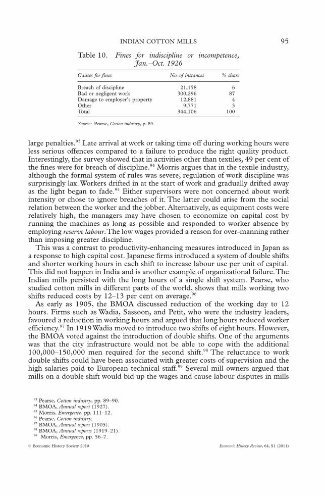
large penalties.93 Late arrival at work or taking time off during working hours wereless serious offences compared to a failure to produce the right quality product.Interestingly, the survey showed that in activities other than textiles, 49 per cent ofthe fines were for breach of discipline.94 Morris argues that in the textile industry,although the formal system of rules was severe, regulation of work discipline wassurprisingly lax.Workers drifted in at the start of work and gradually drifted awayas the light began to fade.95 Either supervisors were not concerned about workintensity or chose to ignore breaches of it. The latter could arise from the socialrelation between the worker and the jobber. Alternatively, as equipment costs wererelatively high, the managers may have chosen to economize on capital cost byrunning the machines as long as possible and responded to worker absence byemploying reserve labour.The low wages provided a reason for over-manning ratherthan imposing greater discipline.

This was a contrast to productivity-enhancing measures introduced in Japan asa response to high capital cost. Japanese firms introduced a system of double shiftsand shorter working hours in each shift to increase labour use per unit of capital.This did not happen in India and is another example of organizational failure.TheIndian mills persisted with the long hours of a single shift system. Pearse, whostudied cotton mills in different parts of the world, shows that mills working twoshifts reduced costs by 12–13 per cent on average.96

As early as 1905, the BMOA discussed reduction of the working day to 12hours. Firms such as Wadia, Sassoon, and Petit, who were the industry leaders,favoured a reduction in working hours and argued that long hours reduced workerefficiency.97 In 1919Wadia moved to introduce two shifts of eight hours. However,the BMOA voted against the introduction of double shifts. One of the argumentswas that the city infrastructure would not be able to cope with the additional100,000–150,000 men required for the second shift.98 The reluctance to workdouble shifts could have been associated with greater costs of supervision and thehigh salaries paid to European technical staff.99 Several mill owners argued thatmills on a double shift would bid up the wages and cause labour disputes in mills

93 Pearse, Cotton industry, pp. 89–90.94 BMOA, Annual report (1927).95 Morris, Emergence, pp. 111–12.96 Pearse, Cotton industry.97 BMOA, Annual report (1905).98 BMOA, Annual reports (1919–21).99 Morris, Emergence, pp. 56–7.

Table 10. Fines for indiscipline or incompetence,Jan.–Oct. 1926

Causes for fines No. of instances % share

Breach of discipline 21,158 6Bad or negligent work 300,296 87Damage to employer’s property 12,881 4Other 9,771 3Total 344,106 100

Source: Pearse, Cotton industry, p. 89.



using a single shift system.100 The BMOA passed a resolution in 1920 prohibitingthe implementation of double shifts.Two firms that introduced a double shift wereexpelled from the association in 1921.101 In his statement to the Industrial Dis-putes Committee, Wadia claimed that the introduction of double shifts hadreduced absenteeism.102 However, double shifts did not become the norm until the1930s. In fact, the BMOA rescinded the resolution of 1920 to allow firms toimplement this system.103 The agency problems associated with the separation offinancial and technical jobs in the cotton mills and the managers’ lack of technicalqualifications may explain the failure of organizational change.

The pressure to increase labour productivity in Bombay mills came with the risein wages during the war. There was a move towards organizational change inBombay cotton mills in the 1920s by standardization of the wage structure. Thestrike of 1928 in Bombay ended with the promise to look into standardization ofwages based on the Lancashire lists.104 Standardization of wages and efficiencygains together were seen as a package. However, there was no consensus amongfirms.105 On the issue of wage cuts, too, there were differences among the mills. Inmills that reduced wages, pay had been below the industry average.106 The moreefficient ones typically did not reduce wages, but tried to raise productivity. In hisrepresentation to the Tariff Board in 1927, Sassoon’s representative producedestimates of savings in the total wage bill with increased workloads and higherwages.107 However, the scale of this change remained small. Only 10,000 workerswere affected by the efficiency schemes.108 If standardized piece rates in Lancashirein the mid-nineteenth century were a mechanism to move to a high wage–higheffort equilibrium, as Huberman suggests,109 then the differential pay structure inBombay mills could have prevented the industry from moving to a high effort–highwage outcome. The evidence for organizational failure is persuasive.

VII

This article has revisited the question of unionization and labour productivity inBombay cotton mills using firm-level data. The view of Wolcott and Clark thatworker militancy prevented efficiency gains in the 1920s is not borne out by theempirical analysis when the regional variation in unionization is considered.110 Onthe contrary, labour productivity was higher in the unionized regions of Bombayand Ahmedabad compared to regions with little union activity. Cotton mills inthese cities used less labour per machine and paid higher wages in 1929. Labouruse per machine was lowest in Bombay, which suggests that worker militancy

100 Chandavarkar, Origins, pp. 353–4.101 BMOA, Annual report (1921).102 ITJ (Jan. 1922).103 BMOA, Annual report (1928).104 Morris, Emergence, pp. 170–2. Lancashire lists refer to standardized piece rates for different categories of

workers.105 Ibid.106 Bombay Labour Office, Wages and unemployment, p. 33.107 Ibid., p. 17.108 Chandavarkar, Origins, pp. 275–6.109 Huberman, ‘Piece rates reconsidered’.110 Wolcott and Clark, ‘Why nations fail’, pp. 397–423.



could not have led to inefficient practices.This conclusion is in line with the modelof wage–effort trade-off, when the firm operates at a suboptimal outcome. Union-ization, through its effect on wages, acted as a spur to efficiency in Bombay cottonmills.

This article also proposes a new explanation for why low wages determined lowlabour productivity in Indian cotton mills in the early twentieth century. Contraryto Clark’s view that cultural preference for low effort explains why wages werelow,111 it has been argued that low wages reflected surplus labour in a predomi-nantly agricultural economy. As the Lewis model predicts, wages in industryremained low and, given the price of capital and labour, managers chose to employmore workers per machine. Low wages reduced managerial incentives to makeproductivity-enhancing changes until there was an exogenous shock to wagesduring the war. The organizational structure of the industry and the separationbetween the managerial and the technical staff and the jobbers may explain thefailure to bring about changes subsequently.

University ofWarwick

Date submitted 9 April 2007Revised version submitted 13 May 2009Accepted 23 June 2009

DOI: 10.1111/j.1468-0289.2010.00528.x

Footnote referencesAllen, S. G., ‘Unionisation and productivity in office building and school construction’, Industrial and Labour

Relations Review, 39, 2 (1986), pp. 187–201.Bagchi, A. K., Private investment in India (Cambridge, 1972).Blyn, G., Agricultural trends in India, 1891–1947: output, availability and productivity (Philadelphia, 1966).BMOA (Bombay Millowners’ Association), Annual reports (1900–38).Bombay, Presidency of, Labour Office, Report on enquiry into wages and hours of labour in the cotton mill industry

(Bombay, 1921, 1923, 1926).Bombay, Presidency of, Labour Office, Wages and unemployment in the Bombay cotton textile industry, Report of the

Departmental Enquiry (Bombay, 1934).Brown, C. and Medoff, J. L., ‘Trade unions in the production process’, Journal of Political Economy, 86 (1978),

pp. 355–78.Buchanan, D., The development of capitalist enterprise in India (1966).Chandavarkar, R., Origins of industrial capitalism in India (Cambridge, 1994).Clark, K. B., ‘Unionisation and productivity: micro-econometric evidence’, Quarterly Journal of Economics, 95

(1980), pp. 613–39.Clark, G., ‘Why isn’t the whole world developed? Lessons from the cotton mills’, Journal of Economic History, 49

(1987), pp. 107–14.Clark, G., ‘Factory discipline’, Journal of Economic History, 54 (1994), pp. 128–63.Clark, G., A farewell to alms: a brief economic history of the world (Princeton, N.J., 2007).Domenech, J., ‘Labour market adjustment a hundred years ago: the case of the Catalan textile industry,

1880–1913’, Economic History Review, 61 (2008), pp. 1–25.Freeman, R. B. and Medoff, J. L., What do unions do? New York: Basic Books. (1984).Hall, R. E. and Jones, C. I., ‘Why do some countries produce so much more output per worker than others?’,

Quarterly Journal of Economics, 114 (1999), pp. 83–116.Huberman, M., ‘Piece rates reconsidered: the case of cotton’, Journal of Interdisciplinary History, 26 (1995),

pp. 393–417.Hunter, J., Women and the labour market in Japan’s industrialising economy: the textile industry before the PacificWar

(2003).

111 Clark, ‘Why isn’t the whole world developed?’, pp. 107–14.



Johnston, B., ‘Agricultural productivity and economic development in Japan’, Journal of Political Economy, 51(1951), pp. 498–513.

Kiyokawa, Y., ‘Technical adaptations and managerial resources in India: a study of the experience of the cottontextile industry from a comparative viewpoint’, Journal of Developing Economies, 21 (1983), pp. 97–133.

Kooiman, D., Bombay textile labour: managers, trade unionists and officials 1918–1939 (Delhi, 1989).Lewis, W. A., ‘Economic development with unlimited supplies of labour’, Manchester School, 22 (1954),

pp. 139–91.Maddison, A., The world economy: a millennial perspective (2001).Madholkar, G.V., ‘The entrepreneurial and technical cadres of the Bombay cotton textile industry between 1854

and 1914: a study in the international transmission and diffusion of techniques’ (unpub. Ph.D. thesis, Univ. ofNorth Carolina, 1967).

Mass, W. and Lazonick, W., ‘The British cotton industry and international competitive advantage: the state of thedebates’, Business History, 32, 4 (1990), pp. 9–65.

Metcalf, D., ‘Unions and productivity, financial performance and investment: international evidence’, inJ. Addison and C. Schnabel, eds., International handbook of trade unions (2003), pp. 118–71.

Morris, M. D., The emergence of an early Indian labour force in India (Berkeley, Calif., 1965).Otsuka, K., Ranis, G., and Saxonhouse, G., Comparative technology-choice in development: the Indian and Japanese

cotton textile industries (1988).Patel, S., The making of industrial relations: the Ahmedabad textile industry, 1918–1939 (Delhi, 1987).Pearse, A., The cotton industry of India (Manchester, 1930).Pollard, S., The genesis of modern management (1965).Rutnagur, S. M., Bombay industries: the cotton mills (Bombay, 1927).Saxonhouse, G. and Wright, G., ‘New evidence on the English mule and cotton industry’, Economic History

Review, 2nd ser., XXXVII (1984), pp. 507–19.Sivasubramoniam S., The national income of India (Delhi, 2000).Thompson, E. P., ‘Time, work discipline and industrial capitalism’, Past and Present, 38 (1967), pp. 56–97.Vicziany, M., ‘The cotton trade and commercial development of Bombay, 1855–1875’ (unpub. Ph.D. thesis,

Univ. of London, 1975).Wolcott, S., ‘Perils of lifetime employment systems: productivity advance in the Indian and Japanese textile

industries, 1920–1938’, Journal of Economic History, 54 (1994), pp. 302–24.Wolcott, S. and Clark, G., ‘Why nations fail: managerial decisions and performance in Indian cotton. Textiles,

1890–1938’, Journal of Economic History, 59 (1999), pp. 397–423.Wright, G., ‘Cheap labour and southern textiles, 1880–1930’, Quarterly Journal of Economics, 96 (1981),

pp. 605–29.Wright, G., ‘Productivity growth and the American labour market: the 1990s in historical perspective’, in

P. Rhode and G. Toniolo, eds., The global economy in the 1990s: a long-run perspective (2006), pp. 139–60.

Official publicationReport of the Indian Tariff Board (1927).



wages, unions, and labour productivity: evidence from ... · wages, unions, and labour...

Documents