wages, rents, and the quality of life - brown university · wages, rents, and the quality of life...

Wages, Rents, and the Quality of LifeAuthor(s): Jennifer RobackSource: Journal of Political Economy, Vol. 90, No. 6 (Dec., 1982), pp. 1257-1278Published by: The University of Chicago PressStable URL: http://www.jstor.org/stable/1830947 .

Accessed: 07/01/2014 13:25

Your use of the JSTOR archive indicates your acceptance of the Terms & Conditions of Use, available at .http://www.jstor.org/page/info/about/policies/terms.jsp

.JSTOR is a not-for-profit service that helps scholars, researchers, and students discover, use, and build upon a wide range ofcontent in a trusted digital archive. We use information technology and tools to increase productivity and facilitate new formsof scholarship. For more information about JSTOR, please contact [email protected].

.

The University of Chicago Press is collaborating with JSTOR to digitize, preserve and extend access to Journalof Political Economy.

http://www.jstor.org

This content downloaded from 128.100.177.16 on Tue, 7 Jan 2014 13:25:36 PMAll use subject to JSTOR Terms and Conditions

http://www.jstor.org/action/showPublisher?publisherCode=ucpress

http://www.jstor.org/stable/1830947?origin=JSTOR-pdf

http://www.jstor.org/page/info/about/policies/terms.jsp


Wages, Rents, and the Quality of Life

Jennifer Roback Yale University

This study focuses on the role of wages and rents in allocating workers to locations with various quantities of amenities. The theory demonstrates that if the amenity is also productive, then the sign of the wage gradient is unclear while the rent gradient is positive. The theory is extended to include the housing market and nontraded goods. These extensions require little modification of the conclusion. The empirical work on wages shows that the regional wage differences can be explained largely by these local attributes. With the use of site price data, implicit prices are estimated and quality of life rankings for the cities are computed.

Introduction

The problem of correctly measuring the implicit price of urban attributes has received much attention in the past decade. Most of the studies have used some variant of the hedonic price method, either estimating wage differentials (Nordhaus and Tobin 1972; Getz and Huang 1978; Rosen 1979) or estimating rent differentials (Ridker and Henning 1967; Polinsky and Rubinfeld 1977). Unfortunately, these studies have focused solely on the consumer side of the market without any regard given to the behavior of firms. For example, if workers require a compensating wage differential to live in a big, polluted, or otherwise unpleasant city, the firms in that city must have

I would like to thank Sherwin Rosen, Elhanan Helpman, and the University of Chicago Applications of Economics Workshop for helpful comments. This material is based on work supported by the National Science Foundation under grant SOC77- 24282. Any opinions, findings, and conclusions or recommendations expressed in this publication are mine and do not necessarily reflect the views of the National Science Foundation. I also benefited greatly from the extensive comments of the referee.

Journal of Political Economy, 1982, vol. 90, no. 6] ? 1982 by The University of Chicago. All rights reserved. 0022-3808/82/9006-0006$01.50

1257



1258 JOURNAL OF POLITICAL ECONOMY

some productivity advantage to be able to pay the higher wage. Indeed, one of the chief insights of Rosen's (1974) theoretical work on hedonic prices is that the implicit price of an attribute represents both the marginal valuation to consumers and the marginal cost to firms. Thus, if one ignores the firm side of the market, the matching aspect of the problem has been lost.

If one seriously considers a full hedonic model of the intercity location problem, one discovers that the problem is much more for- midable than the usual hedonic price problem, because both the land and the labor markets must clear. A simple example will illustrate the difficulty. Suppose all firms and all workers are identical. Then, the usual result is that only one type ofjob or one brand of product will be offered. This presents no problem if the good under consideration is a refrigerator or a car because all consumers may certainly consume the same type of refrigerator if they so desire. However, in the spatial allocation problem, people cannot all occupy the same space even if their preferences are identical. Hence, the scarcity of amenable land gives rise to an additional constraint on the problem. The already difficult problem of solving explicitly for a hedonic price equilibrium becomes all but impossible when two markets must clear simultaneously.

The preceding discussion illustrates two major outstanding problems in this field. First, the role of the interconnected land and labor market-clearing conditions in generating the equilibrium is not well understood. Second, the factors which influence the precise decomposition of the implicit prices into wage and rent gradients have not been determined. The present work addresses these questions by using a general equilibrium model, which incorporates both mobile factors (labor) and site-specific factors (land). It also incorporates the possibility that the amenities may influence productivity.

Previous work in this field illustrates the variety of uses to which the implicit prices may be put. Nordhaus and Tobin (1972), for example, are concerned with the appropriate urban disamenity adjustments to the GNP accounts. Other studies, such as that of Polinsky and Rubin- feld (1977), seek prices for use in cost-benefit studies of particular attributes such as pollution. In still other work, such as Rosen's (1979), the valuations are used as price weights in computing quality of life rankings. All of these issues are addressed below. In particular, the model implies a method for imputing implicit prices from wage and rent regressions. The exact analytic expressions for this decomposition as well as those for adjusting GNP accounts and for evaluating local improvements are discussed.

To clarify issues, the simplest possible model is presented in Section I, while Section II extends the model to include the housing market. Empirical results are reported in the final section. Wage and rent



QUALITY OF LIFE 1259

equations are presented and implicit prices of amenities are calcu- lated. The prices of crime, pollution, and cold weather indicate that these attributes are indeed disamenities, while clear days and, sur- prisingly, population density are found to be amenities. These prices are then used to compute quality of life rankings for the 98 cities used in the study. Although the prices themselves are somewhat sensitive to the specification of the equation due to multicollinearity, the evidence suggests that the city rankings are fairly robust to specification differences. As a by-product of the wage equation, the well-known regional differences in wages are examined and are found to be explained almost entirely by differences in amenities.

I. The Basic Model

Price Determination

Imagine many cities which vary according to the quantity of an en- dowed amenity, s, where s varies continuously over (SI, S2). The possibility that the level of s may be changed by the community is ignored. The residents of each city consume and produce a composite consumption commodity, X, whose price is fixed by world markets and will be taken as numeraire.

The basic framework for all the analysis is a simple general equilibrium model in which both capital and labor are assumed completely mobile across cities. In this context, complete mobility of labor means that the costs of changing residences are zero. Intercity commuting costs are assumed prohibitive to rule out the possibility of a person living in San Diego and working in Chicago. On the other hand, intracity commuting costs are ignored in what follows to focus attention on the across-city allocation of workers and firms.' In contrast, land is fixed2 among cities but is assumed mobile between uses within a city. Given an equilibrium distribution of firms and workers across cities, wage and rent differences can be characterized as functions of s.

1. Workers

Workers are assumed to be identical in tastes and skills.3 For simplic- ity, leisure is ignored and each person supplies a single unit of labor

1 The within-city allocation questions so frequently discussed by urban economists can be addressed easily in the context of this model. In Sec. II of the paper, the relationship between the two models will be discussed.

2 Land need not literally be fixed. We simply need a rising supply price of land in order to assure some boundary on the size of the city. In the more traditional urban economics literature, this rising supply price is provided by the fact that increased city size increases transportation costs. Thus, within-city transport costs provide a natural (although endogenous) boundary on the city size.

3The consequences of this assumption are discussed in the empirical section.




independently of the wage rate.4 The problem for the representative worker is, given the quantity of s in his location, to choose quantities of x, the composite commodity consumed, and iC, the residential land consumed, to satisfy a budget constraint:

max U(x, lC; s) subject to w + I = x + lCr. (1)

The wage and rental payments are denoted by w and r, respectively. Nonlabor income is denoted by I and is assumed to be independent of

5 location. Associated with equation (1) is the indirect utility function, V, with

the usual properties. In addition, 0 V/Os > 0 because s is an amenity. The market equilibrium condition for workers is given by

V(w, r; s) = k. (2)

Wages and rents must adjust to equalize utility in all occupied locations. Otherwise some workers would have an incentive to move.

2. Firms

Assume that X is produced according to a constant returns-to-scale production function, X =f (lP, N; S),6 where lP is land used in production and N is the total number of workers in the city. The problem for the representative firm is to minimize costs subject to the production function. Sincef is constant returns to scale, the unit cost function can be considered. The equilibrium condition for firms is that unit cost must equal product price, assumed to be unity:

C(w, r;s) = 1. (3)

Otherwise, firms would have an incentive to move their capital to more profitable cities. As usual, the unit cost function is increasing in both factor prices. Also, C, = NIX and C, = lP/X.

If the amenity is unproductive, then C, < 0. An example of an "unproductive amenity" is clean air, because firms must spend re-

r This assumption is easily relaxed, with the major conclusions left unchanged. See Roback (1980) for details.

5The implicit land ownership assumption is that each person owns an equal share of land in all cities, regardless of his own location. Although migration patterns will certainly influence the overall level of I, individuals disregard their own effect on rents and hence rental income is independent of location. In the absence of this assumption, (a) capital gains will result from migration flows and (b) people with higher nonwage income (such as retirees) will be found in high s locations, since amenities are normal goods. We abstract from these interesting issues and hence suppress I in what follows.

6 Actually X is a function of capital as well as IP and N. But since capital is perfectly mobile and is uninfluenced by amenities, its rate of return will be equal in all places. Hence, the capital input can be assumed to be optimized out of the problem. The same assumption about the ownership of land applies to the ownership of capital.




r. V(w r;s 2)

C/(w,r;sl)

0 ~~~~~~C( w,r; s21)

W. S1 <S2

FIG. 1

sources to use a nonpolluting technology. An example of a "productive amenity" might be "lack of severe snow storms" because blizzards may be as costly to the firm in inconvenience and lost production as they are unpleasant to consumers. The amenity "sunny days" (with precipitation held constant) probably has no effect on production.

3. Equilibrium

Notice that equations (2) and (3) perfectly determine w and r as functions of s, given a level of k. The equilibrium levels of wages and rents can be solved from the equal utility and equal cost conditions. That is, w and r are determined by the interaction of the equilibrium conditions of the two sides of the market.7 The effects of different quantities of s on wages and rents can be understood with the aid of figure 1.

The downward-sloping lines are combinations of w and r which equalize unit costs at a given level of s. Suppose that s is unproductive so that, for s2 > s1, factor prices must be lower in city 2 to equalize costs in both cities. The duality of C with the production function is that the less substitutable are land and labor, the less the curvature of the factor price frontier. Similarly, the upward-sloping lines represent w-r combinations satisfying V(w, r; s) = k at given levels of s. At

7The market-clearing conditions in the land and labor markets are used to solve for the population gradient and the common level of utility. The utility level then influences the wage and rent gradients, as mentioned in the text. See Roback (1980) for details.




high amenity locations, people must pay higher rents at every wage to be indifferent between the two cities. Again, the more substitution between x and 1c, the greater the curvature of the indirect utility function.

The figure clearly shows that in more amenable places, the wages should be lower while the change in rents is uncertain. The intuitive reason for this is that with s unproductive, firms prefer low s locations while workers prefer high s locations. Because high rents discourage both firms and workers from locating in the area, worker equilibrium requires high rents in high s areas to choke off immigration while firm equilibrium requires low rents in high s areas to induce firm location. On the other hand, a low wage discourages workers and attracts businesses. Essentially, the factor prices are striking a balance between the conflicting locational preferences of the firm and the workers. The reader can easily satisfy himself that if s were productive, the rents would rise while the change in wages would be ambiguous. Also, note that if land is not a factor of production, the wage is determined by the cost function and the rent captures the entire amenity valuation. This is the case considered by Rosen (1979).

These basic results can be obtained algebraically by differentiating equations (2) and (3) and solving for dw/ds and drids. The result is equations (4):

dw I- (-VsCr + CsVr) < Ok ds A (4)

dr I (-VwCs + VSCW) ?0

where A = VwCr - VrCw = L(s)VwIX > 0, and L(s) is the total land available at location s. Using the properties of V and C, we can easily see that with C, > 0, dwlds < 0, while drlds depends on the relative strengths of the productivity and amenity effects.8

Potential Applications

Notice that dwlds and drlds are, in principle, observable. The two equations in (4) express dwlds and drids in terms of the amenity and productivity effects. Hence equations (4) provide a means of imputing

8 Elasticities of substitution do not enter these expressions because small changes are being considered. This result is often found in international trade theory (see Jones 1965).




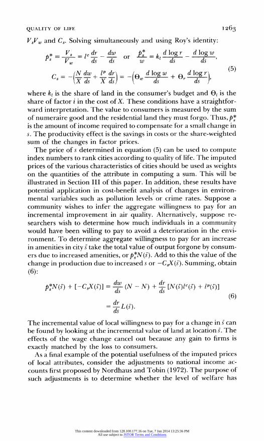
VSVw and C. Solving simultaneously and using Roy's identity:

c dr _ dw dor _ =r d log _ V5 dr dw ors k, lg PS= -(X ds ds w ds ds

N Ndw ?P ldr _ d log w) 0dlogr) (5)

where kl is the share of land in the consumer's budget and Of is the share of factor i in the cost of X. These conditions have a straightfor- ward interpretation. The value to consumers is measured by the sum of numeraire good and the residential land they must forgo. Thus, p* is the amount of income required to compensate for a small change in s. The productivity effect is the savings in costs or the share-weighted sum of the changes in factor prices.

The price of s determined in equation (5) can be used to compute index numbers to rank cities according to quality of life. The imputed prices of the various characteristics of cities should be used as weights on the quantities of the attribute in computing a sum. This will be illustrated in Section III of this paper. In addition, these results have potential application in cost-benefit analysis of changes in environmental variables such as pollution levels or crime rates. Suppose a community wishes to infer the aggregate willingness to pay for an incremental improvement in air quality. Alternatively, suppose researchers wish to determine how much individuals in a community would have been willing to pay to avoid a deterioration in the environment. To determine aggregate willingness to pay for an increase in amenities in city ? take the total value of output forgone by consumers due to increased amenities, or p*N(s). Add to this the value of the change in production due to increased s or -CXX(s). Summing, obtain (6):

p*N(s) + [-C5Xs)] -= dw (N - N) + dr [N(s)lC(s) + lp(S)] (6)

dr

The incremental value of local willingness to pay for a change in ? can be found by looking at the incremental value of land at location s. The effects of the wage change cancel out because any gain to firms is exactly matched by the loss to consumers.

As a final example of the potential usefulness of the imputed prices of local attributes, consider the adjustments to national income accounts first proposed by Nordhaus and Tobin (1972). The purpose of such adjustments is to determine whether the level of welfare has




increased over time, as suggested by conventionally measured GNP accounts, or whether deterioration in the quality of life has offset the gains in output. To find the appropriate measure of welfare, differ- entiate the utility function: Uxdx + U1,dlc + Usds = dk. Or dx + rdlc + (UsIUx)ds = dk/X. The change in utility is simply dkAIX, and this is the conceptually appropriate measure of GNP. The sum dx + rdlc is the change in conventionally measured GNP. The term UsIUx is equal to VIVw. Hence, the adjustment to changes in GNP is simply p*ds, where p* can be inferred from the data using equation (5). This contrasts with the pioneering work of Nordhaus and Tobin (1972), which made the GNP adjustments using only wage differentials.

II. The Housing Market and Other Nontraded Goods

This section extends the simple model by introducing a nontraded- goods sector. Perhaps the most obvious example of a nontradable is housing, but the generalization encompasses the usual nontraded goods such as haircuts and theaters as well. In addition, this extension allows us to consider the possibility that households may modify their own "consumption" of an attribute inherent in their environment through a home production process. Suppose people value the good "comfortable indoor temperature," which can be produced using insulation and fuel, given the outdoor temperature. Or people may reduce their own probability of being robbed by purchasing guard dogs, alarm systems, and police whistles. In both these examples, the good is produced by the household solely for its own consumption and hence is not traded.

The importance of explicitly including the housing market in the analysis is that much work has been done studying the intracity variation in housing prices with amenities. Pollution, crime, racial composition, and access to the central business district have all been shown to have effects on housing prices. The present model allows us to study the decomposition of the housing price gradient into the pure amenity or productivity effects and the effects due to changes in the site price or in the wage. We can also ask whether the difference in housing prices reflects the true implicit price of the amenity.

The generalization for the household requires that the vector of nontraded goods, y, enter into the utility function. We can now consider consumption land, lc, as an input into the production of housing. Land increases utility indirectly through the consumption of housing. We can therefore drop Ic from the utility function, keeping in mind that land for housing is but one element of the vector of land inputs into nontraded-goods production, ly. Land for barbershops and land for theaters as well as land for housing are included in ly.




The demand fory implies a derived demand for land, including what we previously labeled iC.

This generalization implies that the indirect utility function now depends on p, the price of nontraded goods relative to traded goods, but not separately on the rental rate of land:

V(w, p; s) = k. (7)

The production side requires that we introduce a nontraded-goods sector, with the associated unit cost function equated with unit price:

G (w, r; s) = p(s). (8)

Once again, this is a constant-returns-to-scale production function using both land and labor and including s as a neutral shift parameter. Market clearing requires that total output of nontraded goods be equal to total consumption, Ny.

Equations (7) and (8), together with the traded-goods cost function (3), are sufficient to determine w, r, and p. The price-amenity gra- dients9 can be found as before by differentiating and solving simultaneously:

dP *[+Vs(-GCr + GrC) - Cs(GrVw) + Gs(VwCr)], (9)

where A* = VwCr - Vp(CwGr - CrGw) > 0. The change in the price of nontraded goods with respect to a

change in amenities is an expansion of the equation

dp G dw + G dr + G (I0) ds TdS rds s(0

The Vs term in equation (9) is easily interpreted in this context. The first term in parentheses is the effect on p from changes in the wage, while the second term reflects the change inp due to changes in rents. Thus, the Vs term in equation (9) is ambiguous since the amenity effects in the wage and rent gradients have opposite signs.

The productivity effect of s on traded-goods production has an inverse relation to the price of nontraded goods. If s inhibits indus- trial production (Cs > 0), this lowers local factor prices, which indirectly lowers the price of nontraded goods. On the other hand, if s inhibits the production of nontraded goods (Gs > 0), this simply has the direct effect of raising costs. For example, houses are probably more expensive to build in a swamp.

9 The wage and rent gradients are omitted here for brevity. They are simple generalizations of the gradients in the previous section. See Roback (1980) for details.




The upshot of this analysis for empirical work is clear: Predictions about cross-city variation in housing prices are more difficult to make than those about variation in land prices. However, studies such as those by Ridker and Henning (1967) and Polinsky and Rubinfeld (1977) which examine intracity housing prices have been successful in finding higher housing values associated with amenities such as clean air or downtown accessibility. This is because in these models, housing prices more closely mirror site values. Two sources of ambiguity in the present model are removed when considering intracity price differences. First, within-city differences in productivity in the housing industry are likely to be negligible. Second, although the amenities are consumed jointly with housing, ajob can be held anywhere in the city. Thus, wages of identical individuals must be independent of location.10 Since land rents are higher in good locations and wages are constant across locations, the price of housing rises unambiguously with s because the price of housing is simply a sum of these two factors. Note that a good location in this context may be the much- studied proximity to the central business district. This shows the strong relationship between the present analysis of intercity quality variation and the more traditional problem of intracity amenity differences.

Finally, we can derive the amenity effects and the productivity effects of s by differentiating the three equilibrium conditions and using Roy's identity:

* _ Vs dp dw V ds ds

dw dr Cs = -t ~ + C, s

dw dr (Gwy?- +Gr#). w ds rdJ

These equations illustrate how the applications discussed in the previous section extend to the more general model. Again, p* tells the change in numeraire income required to compensate for a small variation in s. In general, the housing price gradient will not capture the full valuation of the amenities. An adjustment for the differences in wages must be included.

10 This abstracts from the stratification of workers across locations due to income effects.




w.

AO

! ~~~IA

SI S2 S

FIG. 2

III. Empirical Results

The Relation of Empirical Work to Theory

The theory developed earlier assumes that all individuals have identical tastes and skills. Because tastes for amenities differ among people in the data, however, we expect those with stronger preferences for amenities to sort themselves into more amenable places and be willing to accept a lower wage.1' Those with weaker preferences will be willing to accept a lower wage than their co-workers to go without the amenity and hence will be found in less pleasant cities. Therefore, the estimated wage difference will be an underestimate of the true equalizing wage difference for those with strong tastes for amenities and an overestimate for those with weak preferences. A similar argument can be made for biases in the estimated rent gradient."2

Figure 2 illustrates the wage bias graphically. Type A consumers have stronger preferences for amenities than type B consumers. Points A and B will be observed in the data and hence will define the market-equalizing wage difference. However, points A and A' define the true equalizing difference for type A consumers while the wage difference associated with points B and B' is the equalizing difference for type B consumers. Clearly, the difference between the wages at A and B lies between the true equalizing differences for each group.

11 We continue to assume that the amenities are well defined so that the possibility of some people preferring cold weather can be thought of as weak preferences for warm weather.

12 This self-sorting bias arises in all hedonic price problems (see Rosen 1974).




Notice that even with perfect sorting of an infinite variety of consumers, differentials will be observed. The observed wage gradient is the lower envelope of the individual consumer gradients. Because these gradients are convex to the origin and downward sloping, their lower envelope will also be negatively inclined. Hence, because taste differences exist in the data, the estimates presented below are a kind of average of the true gradients for the various groups. A comparable argument can be made for productivity differences and relative factor intensities for firms.

Workers who differ in skills compete in separate markets. Each group will have its own wage-amenity gradient. In earlier work,13 the data were segmented by broad skill groups. Space limitations pre- clude discussion of this extensive material. In the work reported below, productivity traits are entered into the individual wage equations. This procedure allows the gradients to be shifted by productivity indicators but forces the slopes of the wage-amenity gradients to be the same for all skill levels.

Before discussing results, I should mention two other caveats. First, the choice of which city attributes to include is a matter of discretion. We do not know a priori which goods people value, and so we must seek this information from the data. Viewed another way, theory does not tell us which attributes are goods; theory only tells us how people behave with respect to goods. For this reason, extensive experimenta- tion was done with many variables. Second, the small number of observations and high degree of multicollinearity among the variables limited the number of different indicators which could be used. For instance, when several climate variables are entered into the same earnings regression, none is significant. Yet one might have thought that both the number of hot days and the precipitation would be relevant to location decisions. Also, some of the results are sensitive to alternative specifications. The equations reported below were chosen to be representative of the bulk of the results and to be demonstrative of the type of behavior described by the theory.

The Data and Results

The principal source of wage data for this study is the Census Bureau's Current Population Survey from May 1973. The May data identify individuals in the 98 largest U.S. cities, which allows many more degrees of freedom and much more detailed productivity information than are commonly found in studies of this problem. The

13 Roback (1980) segmented data according to occupation and schooling groups. Getz and Huang (1978) separated by occupation.




study was confined to men over 18 who reported earnings and who lived in one of the identified cities.

Perhaps the only source of data on residential site prices across cities is found in FHA Homes (U.S. Department of Housing and Urban Development 1973), which reports average site prices per square foot for 83 of the 98 largest cities. Because the data are collected only for FHA-qualifying families, low-income families are overrepresented relative to the population used in the wage study. Also, no information about the location of the site within the city is available. Because of these limitations of the data, the land price results presented below are merely intended to be illustrative of the method outlined in the theory.

1. Wage Results

The Appendix table shows the regression of personal characteristics on the log of weekly earnings.'4 Examination of the table shows that these variables include all of the usual individual attributes known to influence wages. This detailed information on worker traits is the chief advantage of using this micro data set. In addition to these usual variables, industry dummies were included to hold constant the in- dustrial composition of the city. The poverty incidence variables tell the percentage of the person's neighborhood which is below the poverty line. This variable was included as a crude control on the within-city differences in amenities. It may capture differences in family background and schooling quality as well. The effects of these variables changed little when they were included in the subsequent regressions of wages on city attributes.

Table 1 presents the results of five regressions of various city traits on log earnings for this full sample of 98 cities. Looking across a row gives some indication of the robustness of a variable to different specifications. For example, rows 1 and 3 show that the total crime rate (TCRIME 73) and the particulate level (PART 73) always have the expected positive influence on wages, but this influence is not always statistically significant. The coefficient on the local unemployment rate (UR 73) is always insignificant, which suggests either that the required risk premium for living in a high unemployment area is small or that a high unemployment rate is a proxy for weak local labor demand. This contrasts with the result of Hall (1972), who found high

14 Throughout this paper, nominal earnings is used as the dependent variable because price-level information is available for only 32 of the 98 cities. However, including the price level alters the results reported below only in that heating degree days is insignificant and population density is significantly negative.



1 270 JOURNAL OF POLITICAL ECONOMY

TABLE 1

COEFFICIENTS OF CITY CHARACTERISTICS FROM LOG EARNINGS REGRESSIONS IN 98 CITIES

1 2 3 4

TCRIME 73 .94 X 10-5 .44 x 10-5 .74 X 10-5 .86 x 1O-5 (2.58) (1.17) (1.93) (2.21)

UR 73 .36 x 10-2 .12 x 10-2 .32 x 10-2 .27 x 10-2 (1.29) (.43) (1.14) (.97)

PART 73 .24 x 10-3 .13 x 10-3 .37 x 1O-3 .34 x 10-3 (1.55) (.86) (2.33) (2.15)

POP 73 .16 x 10-7 .15 x 10-7 .16 x 10-7 .16 x 10-7 (7.97) (7.74) (8.04) (8.11)

DENSSMSA .81 x 10-6 .24 x 10-5 .20 x 10-5 .38 x 10-5

(.29) (.86) (.73) (1.40) GROW 6070 .21 x 10-2 .14 x 10-2 .15 x 10-2 .17 x 10-2

(7.84) (5.66) (6.06) (6.47) HDD .20 x 10-4

(8.48) TOTSNOW .72 x 10-3

(3.54) CLEAR -.64 x 10-2

(-4.80) CLOUDY .72 x 10-2

(5.21)

R 2 .4980 .4955 .4960 .4962 F-ratio 424.2 420.0 420.8 421.1 N = 12,001

NOTE.-Regressions include all personal characteristics. Sample includes 98 cities; t-statistics are in parentheses (see App. for variable definitions).

wages associated with high unemployment. Population size and the population growth rate both have the expected strong positive effects while population density (DENSSMSA) is consistently insignificant.

The climate variables in table 1 perform remarkably well. Heating degree days (HDD), total snowfall (TOTSNOW), and the number of cloudy days (CLOUDY) all have strong positive coefficients, which suggests that these indicators of climate are net disamenities. The number of clear days (CLEAR) has a strongly negative coefficient, which is consistent with the prior notion that clear days are amenable.15

The next question to be addressed is: What is the influence of the city attributes on the well-known regional differences in earnings? These persistent region effects have always been something of a puzzle because a mobile labor force ought to bid away any geographic differences in real earnings. Because "real earnings" should be defined broadly to mean utility, we test the hypothesis that the ob-

15 For other results on climate, see Hoch (1977).




TABLE 2

COEFFICIENTS OF REGION DUMMIES AND CITY CHARACTERISTICS

NORTHEAST -.0218 -.0095 (-2.25) (-.74)

SOUTH -.0669 -.0138 (-6.51) (-.87)

WEST -.0354 -.0579 (-3.46) (-3.41)

TCRIME 73 .13 x 10-4 (2.82)

UR 73 .92 x 10-2 (2.60)

PART 73 .29 x 10-3 (1.87)

POP 73 .16 x 10-7 (7.77)

DENSSMSA .13 x 10-5 (-.42)

GROW 6070 .23 x 10-2 (8.41)

HDD .16 x 10-4 (4.86)

R 2 .4900 .4986 F-ratio 479.4 384.0

NOTE.-Regressions include all personal characteristics. Sample includes all 98 cities; I-statistics are in parentheses.

served earnings differentials are in fact proxies for different amenity levels. The first column of table 2 presents evidence of the existence of regional effects in these data.16 The t-statistics on all three of the regional dummies indicate significant differences in wages across regions. Furthermore, an F-test of joint significance of these three variables (comparing eq. 1 of table 2 with the equation in the Appen- dix) gives an F-value of 14.87 where the critical F-value is 1.88.

We expect that the inclusion of various measures of city attractive- ness may considerably diminish the effect of region per se. A comparison of columns 1 and 2 of table 2 gives some support for this idea. The coefficients on the northeastern and southern dummies fall dramatically, and the t-statistics indicate no difference in wages between these two regions and the Midwest. The persistent strength of the western effect is the only anomaly in this pattern. It is certainly correct to infer from these results that earnings are lower in the West than elsewhere. However, once differences in amenities are taken into account, region plays a greatly reduced role in explaining earnings. The fact that low wages in the West are accompanied by extremely

16 For further evidence of and debate about the effect of region, see Coelho and Ghali (1971) and Ladenson (1973).



1 272 JOURNAL OF POLITICAL ECONOMY

TABLE 3

REGRESSIONS OF THE LOG OF AVERAGE RESIDENTIAL SITE PRICE PER SQUARE FOOT ON CITY CHARACTERISTICS

1 2 3 4

TCRIME 73 2.5 x 10-5 1.5 x 10-5 -4.5 x 10-7 7.0 x 10-6 (.65) (.38) (-.01) (.16)

UR 73 8.9 x 10-2 8.8 x 10-2 9.2 x 10-2 9.1 X 10-2 (3.45) (3.35) (3.53) (3.52)

PART 73 2.2 x 10-4 1.1 X 10-4 -3.8 x 10-5 1.4 x 10-4 (.15) (.08) (-.02) (.09)

POP 73 6.8 x 10-8 6.9 x 10-8 6.8 x 10-8 6.8 x 10-8 (1.80) (1.78) (1.76) (1.76)

DENSSMSA 1.9 X 10-4 2.0 x 10-4 2.0 x 10-4 2.0 x 10-4 (3.02) (3.12) (3.17) (3.18)

GROW 6070 1.1 X 10-2 1.0 X 10-2 9.9 X 10-3 1.0 X 10-2 (4.34) (4.11) (4.03) (4.00)

HDD 3.5 x 10-5 (1.44)

TOTSNOW 1.3 x 10-3 (.69)

CLEAR 1.2 x 10-4 (.09)

CLOUDY 3.2 x 10-4 (.21)

INTERCEPT -1.73 -1.54 -1.44 -1.53 (-5.92) (-5.99) (-6.51) (-3.32)

R2 .5741 .5650 .5623 .5625 F-ratio 14.44 13.92 13.77 13.78

SOURCE.-Data are from U.S. Department of Housing and Urban Development 1973. N = 83.

high growth rates of population suggests that living in the West may be a proxy for some unmeasured desirable climatic or cultural attributes. Thus, the combined evidence seems persuasive that the regional differences in earnings can be largely accounted for by regional differences in local amenities.17

2. Implicit Prices and Quality of Life Indices

Table 3 presents the results of a series of land price equations comparable to those in table 1. The only significant results are the positive coefficients on the unemployment rate, population density, and population growth. The latter two results are most likely demand effects, which proxy for some unmeasured attributes of the city. The theory suggests that the land price gradient reveals the marginal social value of the amenity to the community. The reader may be

17 This result is robust to the inclusion of measures of cost of living (see Roback 1980).




tempted to infer from the zero coefficients on crime and pollution that these conditions have no social disutility. The limitations of the data discussed earlier make such a conclusion premature.

To compute the implicit price of each attribute in percentage terms, we need the coefficients from tables 1 and 3, as well as the budget share of land. This budget share was computed from the FHA data by multiplying the fraction of income spent on the mortgage (approximately 17.8 percent) by the ratio of the site price to the total value of the house (approximately 19.6 percent). This number was then aver- aged over all 83 FHA cities to yield an average budget share. Table 4 reports the implicit prices computed from the columns of tables 1 and 3. For example, column 2 reports the prices computed from regressions, which include total annual snowfall as the climate variable. A negative number indicates a "bad" while a positive number indicates a good. While most of the variables perform as expected, looking across the rows of table 4 reveals some sensitivity of the prices to specification.

Each entry in table 4 tells the marginal price of the amenity evaluated at average annual earnings. For example, the average person

TABLE 4

IMPLICIT PRICES OF AMENITIES COMPUTED FROM TABLES 1 AND 3

1 2 3 4

TCRIME 73 (crimes/100 population) $-9.25 $ .90 $ -8.05 $ -9.15

UR 73 (fraction unemployed) -5.55 20.65 -.70 5.00

PART 73 (micrograms/cubic meter) -2.50 -1.40 -4.00 -3.70

POP 73 (10,000 persons) -1.50 -1.40 -1.50 -1.50

DENSSMSA (100 persons/square mile) 6.30 4.90 5.35 3.35

GROW 6070 (percentage change in population) -1.85 -11.95 -13.05 -15.2

HDD (10 F colder for one day -.20

TOTSNOW (inches) -7.30

CLEAR (days) 69.55

CLOUDY (days) -78.25

NOTE.-Measurement units of amenities shown under variable name. Each entry is computed using eq. (5) in the text and evaluated at mean annual earnings.p* = [k1(d logrlds) - (d logw/ds)]w. Average annual earnings = $10,868. Average budget share of land = .035. Negative numbers indicate disamenities, while positive numbers indicate amenities.




TABLE 5

RANK CORRELATIONS BETWEEN VARIOUS MEASURES OF QUALITY OF LIFE INDEX

QOL I QOL 2 QOL 3 QOL 4

QOL 1 1.000 .7846 .2480 .2902 (.0) (.0001) (.0138) (.0037)

QOL 2 1.000 .3568 .2701 (.0) (.0003) (.0072)

QOL 3 1.000 .8219 (.0) (.0001)

QOL 4 1.000 (.0)

NOTE.-Probabilities in parentheses. The indices are computed from cols. 1-4 of tables 2 and 6. Thus QOL 1 uses HDD, QOL 2 uses TOTSNOW, QOL 3 uses CLEAR, and QOL 4 uses CLOUDY.

would be willing to pay $69.55 per year for an additional clear day and $78.25 per year to avoid an additional cloudy day. Some of the entries appear to be small; this is only because of the units of measurement. For instance, the implicit price of a heating degree day is only $0.20, but the average number of heating degree days in the sample is 4330.69 (see Appendix for means). If we evaluate the ''expenditure"' on heating degree days at the mean value and the marginal price, the total implicit expenditure is $866.14. This procedure is not strictly correct, of course, because the prices of infra- marginal units are different from the marginal price. Such an expenditure computation merely shows the order of magnitude of expenditure in the average budget.

As noted in the theoretical section, these prices can be used to compute quality of life indices. Four sets of indices were computed and labeled QOL 1-QOL 4 to represent the columns of table 4. Table 5 reports the rank correlation coefficients for these four rankings. The correlations are all reasonably large, although, as may have been expected from the different climate variables, QOL 1 and QOL 2 are highly correlated with each other, as are QOL 3 and QOL 4. To give the flavor of the results, table 6 lists the 20 largest cities ranked according to QOL 3, which seems to be most highly correlated with the other rankings.

Ben-Chieh Liu (1976) also computed quality of life indices in his study. Rather than using imputed prices as weights for the characteristics, he arbitrarily assigned weights, which have no interpretation as willingness to pay for an attribute. Table 6 presents his rank orderings of the 20 largest cities, based on his environmental index. His rankings differ substantially from QOL 3, partly because he used somewhat different characteristics and partly because of the arbitrary




TABLE 6

COMPARISON OF QOL 3 RANKINGS OF 20 LARGEST CITIES WITH RANKING OF LIu

Liu's Population Rank Name Rank QOL 3 Rank

1 Los Angeles-Long Beach 10 1.7517 2 2 Anaheim-Santa Ana-Garden Grove 9 1.7363 19 3 San Francisco-Oakland 2 1.5841 6 4 Dallas 5 1.3378 17 5 Baltimore 13 1.0244 12 6 Nassau-Suffolk . . . 1.0010 9 7 St. Louis 16 .9407 11 8 Milwaukee 8 .9386 20 9 Boston 12 .9296 8

10 Minneapolis 4 .9047 16 11 New York 14 .8962 1 12 Washington, D.C. 3 .8910 7 13 Newark 11 .8853 15 14 Philadelphia 7 .8038 4 15 Houston 6 .7708 14 16 Chicago 18 .7416 3 17 Detroit 17 .6347 5 18 Cleveland 15 .6227 13 19 Seattle-Everett 1 .5871 18 20 Pittsburgh 19 .4961 10

NOTE.-Liu's rank is based on adjusted standardized score of environmental component. Nassau-Suffolk is not included in Liu's (1976) study.

weights. The method in the present study is conceptually superior, even though the rankings may not accord with prior notions about relative desirability of cities.

IV. Conclusion

This study has proven that the conventional wisdom which holds that only land prices are affected by local amenities is incorrect. The theory demonstrated that the value of the amenity is reflected in both the wage and the rent gradient. The precise decomposition depends on the influence of the amenity on production and the strength of consumer preferences.

The empirical work on wages found that the well-known regional wage differences can be explained largely by local amenities. The empirical part of this study can be extended in a variety of directions. The most important extension is to refine the site price data. Hedonic studies of housing markets should be done to infer the price of the land independent of the housing structure. In addition, more work could be done to segment the data by skill groups. Separate quality of life indices could be computed for each skill group. The correlations




between these rankings for separate groups would be interesting. All of this work would continue to broaden our understanding of the empirical implications of location theory.

Appendix A

Regression of Log of Weekly Earnings on Personal Characteristics

Coefficient t-Statistic

Intercept 3.7418 105.60 Household head .1457 9.94 White .0272 2.14 Married .0776 6.86 Veteran .0274 3.07 School .0446 28.52 Experience .0285 26.57 Experience squared -.0005 -24.85 Hours .0101 20.42 Part time -.2869 -17.90 Private .0129 .89 Professional .3263 24.48 White collar .1189 8.51 Blue collar .1092 9.52 Poverty incidence -.9063 -18.05 Construction .1333 6.19 Durables -.0519 -2.52 Nondurables - .0589 -2.69 Transport .0192 .90 Trade -.1463 -7.22 Services -.2085 -11.49 Union .1213 14.70

NOTE.-Data are from the May 1973 Current Population Survey; R2 = .488 1; F-ratio = 543.9; N = 12,001. The omitted occupation is laborers; the omitted industry is public administration.

Appendix B

Notes on City-wide Variables

1. TCRIME 73: total crimes per 10,000 population for 1973. Source: FBI Uniform Crime Reports (1973). Mean = 5026.04

2. UR 73: unemployment rate in 1973. Source: Manpower Report of the President (1975). Mean = 4.9716

3. PART 73: micrograms/cubic meter of particulates in 1973. Source: EPA Air Quality Data (1973). Reports average pollution level from a number of monitoring stations within each city. Variable used is a weighted average of all stations in the city, with the number of observations taken by the station as weights. Mean = 92.55413

4. POP 73: SMSA population in 1973. Source: Statistical Abstract (1975). Mean = 2,866,958.

5. DENSSMSA: population density of the SMSA in 1973. Source: Statisti- cal Abstract (1975). Mean = 1494.913.




6. GROW 6070: percentage change in population from 1960 to 1970. Source: U.S. Census of Population (1970). Mean = 19.97176.

7. All climate variables taken from local climatological data. All data are "climatological normals," i.e., 30-year averages. (a) HDD: heating degree days; sum of daily negative departures from 65? per year; mean = 4330.69. (b) TOTSNOW: total annual snowfall in inches; mean = 23.616. (c) CLEAR: number of clear days; mean = 109.4529. (d) CLOUDY: number of cloudy days; mean = 146.9858.

References

Coelho, Philip R. P., and Ghali, Moheb A. "The End of the North-South Wage Differential." A.E.R. 61 (December 1971): 932-37.

."The End of the North-South Wage Differential: A Reply." A.E.R. 63 (September 1973): 757-62.

Getz, Malcolm, and Huang, Y. C. "Consumer Revealed Preference for En- vironmental Goods." Rev. Econ. and Statis. 60 (August 1978): 449-58.

Hall, Robert E. "Turnover in the Labor Force." Brookings Papers Econ. Activity, no. 3 (1972), pp. 709-56.

Hoch, Irving. "Variations in the Quality of Urban Life among Cities and Regions." In Public Economics and the Quality of Life, edited by Lowdon Wingo and Alan Evans. Baltimore: Johns Hopkins Univ. Press (for Re- sources for the Future), 1977.

Jones, Ronald W. "The Structure of Simple General Equilibrium Models." J.P.E. 73, no. 6 (December 1965): 557-72.

Ladenson, Mark L. "The End of the North-South Wage Differential: Com- ment." A.E.R. 63 (September 1973): 754-56.

Liu, Ben-Cheih. Quality of Life Indicators in U.S. Metropolitan Areas: A Statistical Analysis. New York: Praeger, 1976.

Nordhaus, William D., and Tobin, James. "Is Growth Obsolete?" In Economic Research: Retrospect and Prospect. Vol. 5. Economic Growth. New York: Colum- bia Univ. Press (for Nat. Bur. Econ. Res.), 1972.

Polinsky, A. Mitchell, and Rubinfeld, Daniel L. "Property Values and the Benefits of Environmental Improvements: Theory and Measurement." In Public Economics and the Quality of Life, edited by Lowdon Wingo and Alan Evans. Baltimore: Johns Hopkins Univ. Press (for Resources for the Fu- ture), 1977.

Ridker, Ronald G., and Henning, John A. "The Determinants of Residential Property Values with Special Reference to Air Pollution." Rev. Econ. and Statis. 49 (May 1967): 246-57.

Roback, Jennifer. "The Value of Local Urban Amenities: Theory and Mea- surement." Ph.D. dissertation, Univ. Rochester, 1980.

Rosen, Sherwin. "Hedonic Prices and Implicit Markets: Product Differentia- tion in Pure Competition." J.P.E. 82, no. 1 (January/February 1974): 34-55.

. "Wages-based Indexes of Urban Quality of Life." In Current Issues in Urban Economics, edited by Peter Mieszkowski and Mahlon Straszheim. Baltimore: Johns Hopkins Univ. Press, 1979.

U.S. Bureau of the Census. Census of Population. Vol. 1, pt. 1. Washington: Bureau of the Census, 1970.




. Current Population Survey. Washington: Bureau of the Census, 1973.

. Statistical Abstract of the United States. Washington: Government Print- ing Office, 1975.

U.S. Department of Housing and Urban Development. FHA Homes. Wash- ington: Housing Production and Mortgage Credit, FHA, 1973.

U.S. Department of Labor. Manpower Report of the President. Washington: Government Printing Office, 1975.

U.S. Environmental Protection Agency. Air Quality Data: Annual Statistics. Annual Summary. Washington: Government Printing Office, 1973.

U.S. Federal Bureau of Investigation. Uniform Crime Reports for the United States. Washington: Government Printing Office, 1973.



wages, rents, and the quality of life - brown university · wages, rents, and the quality of life...

Documents