Wage Cyclicality Revisited:

The Role of Hiring Standards∗

Sekyu Choi

University of Bristol

Nincen Figueroa

Diego Portales University

Benjamın Villena-Roldan

Diego Portales University and MIPP

February 2020

Abstract

We study the cyclicality of online posted wages at the job level, using a

representative dataset for the Chilean economy. Unlike other datasets, ours has

wage and requirements for most job ads. We find clear evidence of posted wage

procyclicality, in line with matched employer-employee studies. Our results

are robust to cyclical mismatch and job upgrading biases, important issues in

the literature. We also show that not controlling for requirements leads to the

underestimation of the cyclicality of offered wages. Indeed, using the Gelbach

(2016) decomposition, we show that ignoring countercyclical experience and

education requirements dampens wage cyclicality estimates.

Keywords: Wage cyclicality, online job boards, composition bias, hiring standards.

JEL Codes: E24, J64

∗Email: sekyu.choi@bristol.ac.uk , nincen.figueroa@gmail.com, and ben-jamin@benjaminvillena.com. We are grateful to Arpad Abraham, Guido Menzio, MortenRavn and our colleagues at the 2019 Annual Search and Matching workshop in Oslo, Norway;the Tinbergen Institute; and the 2019 Chilean Economic Society Meeting for useful commentsand discussions. Villena-Roldan thanks for financial support the FONDECYT project 1191888,Proyecto CONICYT PIA SOC 1402, and the Institute for Research in Market Imperfections andPublic Policy, ICM IS130002, Ministerio de Economıa, Fomento y Turismo de Chile. We aregrateful to www.trabajando.com which provided the raw data used in this paper. All errors areours.

1

1 Introduction

A large debate in macroeconomics concerns the sensitivity of wages to business cycle

fluctuations. Recently, the “unemployment volatility puzzle” (Shimer, 2005; Hall,

2005; Hagedorn and Manovskii, 2008; Costain and Reiter, 2008) states that the widely

used Nash bargaining wage-setting mechanism in the Diamond-Mortensen-Pissarides

framework is unable to explain large fluctuations of unemployment in the data. As

Hall (2005) and Shimer (2010) emphasize, wage rigidity would help reconcile evidence

and theory: Intuitively, productivity shocks would affect profits much more than

wages, triggering a larger response of vacancies and therefore, job creation.

Nevertheless, Pissarides (2009) shows that the relevant wage for job creation is the

one paid to newly hired workers. Moreover, he summarizes existing results showing

that wages for job movers are substantially procyclical, implying that the wage stick-

iness proposed by Hall and Shimer cannot be the reason behind high unemployment

volatility. Gertler and Trigari (2009) provide an alternative interpretation of the evi-

dence highlighted by Pissarides (2009): job composition quality is procyclical, so that

high-quality jobs, paying higher wages appear much more frequently in booms than

in recessions, so that the empirical wage cyclicality is partly due to a composition

bias. A number of papers attempt to assess the relevance of this claim. Haefke et al.

(2013), using CPS data, and Carneiro et al. (2012); Martins et al. (2012); Stuber

(2017) and Dapi (2019) using matched employer-employee databases, conclude, after

accounting for composition in their datasets, that wages of newly hired workers are

highly procyclical.

In this paper we use ten years of data from www.trabajando.com, an internet

job board operating in the Chilean economy. We have access to information on job

ads and offered wages, which are point estimates of what employers expect to pay

to a prospective match. In the website, employers must enter a wage when posting

the advert, but are allowed to hide this information from job seekers. While only a

small fraction posts wages publicly, we observe offered wages for around 85% of the

ads (both hidden and public), a unique feature to the best of our knowledge. Banfi

and Villena-Roldan (2019) show that hidden wages are nearly as informative as the

2

explicit ones. We provide additional evidence here on the representativeness of our

dataset to the Chilean labor market on several dimensions.

Thanks to the richness of our dataset, our first contribution is to estimate the

cyclical sensitivity of wages, controlling not only for the composition of employers

and job titles, as done by previous research, but also for a rich set of contract terms

and hiring standards. Using the later variables such as requirements of education,

major (for jobs requiring a university degree), experience, etc., we can reliably control

for job quality. This is a measurement advantage with respect to other data in which

requirements are obtained through text mining algorithms, with some misclassifica-

tion error. With our data, we are close to run an ideal thought experiment: consider

a firm offering a wage for a job, with specific requirements and contract terms in a

recessive labor market. Keeping all of these constant, let the firm post again a wage

for the same job ad in a booming market, so we can compare and assess the cyclicality

of the offered wage.

A second contribution is subtle but important. All previous papers in the liter-

ature (with the exception of Hazell and Taska (2019), to the best of our knowledge)

draw their conclusions from realized wages, which may be affected by cyclical mis-

match between workers and jobs (Sahin et al., 2014), leading to cleansing or sullying

effects of recessions. Suppose that, in a recession, workers start applying for jobs they

are unfit for due to the scarcity of opportunities and larger unemployment durations.

Realized matches of poor quality lead to lower wages and shorter expected tenures,

as in Oreopoulos et al. (2012). Gertler et al. (2016) also make the case for counter-

cyclical match quality. Most of the existing research control for worker fixed effects,

but this is not enough since these measure the average wage an individual gets in

a typical job. We address the lack of measurement of match quality since our data

consists of offered wages before matches form. Thus, we can ignore concerns about

cyclical quality of the match while also controlling for the ex ante quality of the job

itself. Further, we do not have the problem of trying to disentangle cyclicality of

wages from labor income, since we concentrate our analysis on base wages and can

clearly identify full/part time jobs.1

1According to Swanson (2007), a great deal of cyclicality of wages is accounted for variable labor

3

Due to the features of our data, we are able to directly address the concerns

of cyclical job quality and mismatch, only partially responded in the literature by

firm- and worker-fixed effects models. The paper closest to ours is Hazell and Taska

(2019), who study posted wages from the U.S. economy collected by Burning-Glass

Technologies (BGT). However, in their data only 10% of ads post wages, which likely

entails an overrepresentation of unskilled jobs as shown by Brencic (2012); Banfi and

Villena-Roldan (2019). Also, nearly half of their wage data comes in the form of wage

brackets, which probably overstates their cyclical rigidity.

From our preferred specification, when we control for requirements, job titles and

firm fixed effects, we find significant procyclical offered wages. Our estimated semi-

elasticity of wages with respect to unemployment falls in the upper range of (absolute

value) estimates previously found in the literature: −1.576, which is close to Albagli

et al. (2017) who estimate a range between −1.7 and −2.0 for the Chilean economy.

These numbers are not far from estimates for other countries. On the lower spectrum

of estimates, Gertler and Trigari (2009) find a semi-elasticity of −0.33, while Hazell

and Taska (2019) report a comparable estimate of −0.95.

Furthermore, using the Gelbach (2016) decomposition, we show that requirements

related to high wages are countercyclical. This finding connects our paper to the

literature on the cyclicality of job requirements.2 Data from online job ads has allowed

researchers to study the cyclicality of requirements to explain the well-known outward

shift of the Beveridge curve in the aftermath of the Great Recession. In line with our

own findings, using BGT job ads Modestino et al. (2016, 2020) report that educational

and experience requirements move countercyclically, even for job titles within the

same firm, which helps explain the Beveridge curve shift. Following a macro approach,

Sedlacek (2014) can partially explain the same fact by introducing job requirement

as an employer choice.

Using the Gelbach (2016) decomposition, we measure how much the cyclicality

of wages is underestimated if the countercyclical behavior of job requirements is not

considered, as is the case of previous studies. Although in this paper we primarily

income such as bonuses, overtime, and commissions.2For old discussions on this topic, see Reder (1964); McGregor (1978).

4

concern about the cyclicality of wages, a rigourous analysis necessarily requires an as-

sessment of the cyclical interdependent movements of wages and requirements within

an occupation, and even at the job title and firm level. So far, the wage and require-

ment cyclicality literatures have evolved without realizing their close relationship.

The key intuition is simple: an increased hiring standard in a recession masks the

reduction of offered wages, leading to an underestimation of the procyclical behavior

of wages.

Taken at face value, our estimated semi-elasticity of wages with respect to unem-

ployment implies that the assumption of wage rigidity, needed to explain unemploy-

ment fluctuations in sequential search and matching models along the lines of Shimer

(2005), is not warranted by the data. However, our results reveal a more complex pic-

ture. Employers are more demanding on qualifications when the labor market is weak,

and viceversa. The business cycle affects labor quality, wages, and match probability

margins, even within the same firm and job. In light of this evidence, joint cyclicality

of wages and requirements should be studied together empirically and theoretically.

Baydur (2017); Carrillo-Tudela et al. (2018) take a first step in later direction.

2 Data

We use information from the private job board www.trabajando.com. We have data

on job advertisements posted online between March 1st 2009 and August 31st 2018.

Job postings in the website represent a wide array of sectors, although it concentrates

slightly on retail, services, and manufacturing sectors. Job seekers can use the website

for free, while firms pay to display ads for 30 to 60 days.

The main advantage of the information from this job board is that employers are

required to provide an estimated net monthly salary to be paid at the position.3 Thus,

we have access to offered wage data which is not influenced by characteristics of any

individual worker. The current setup has additionally a number of advantages: the

wage information we analyze does not consider bonuses or other payments workers

may receive which may be subject to aggregate conditions as suggested by Swanson

3It is customary in the Chilean labor market to express wages in monthly terms, net of taxes,social security and health contributions.

5

(2007).4

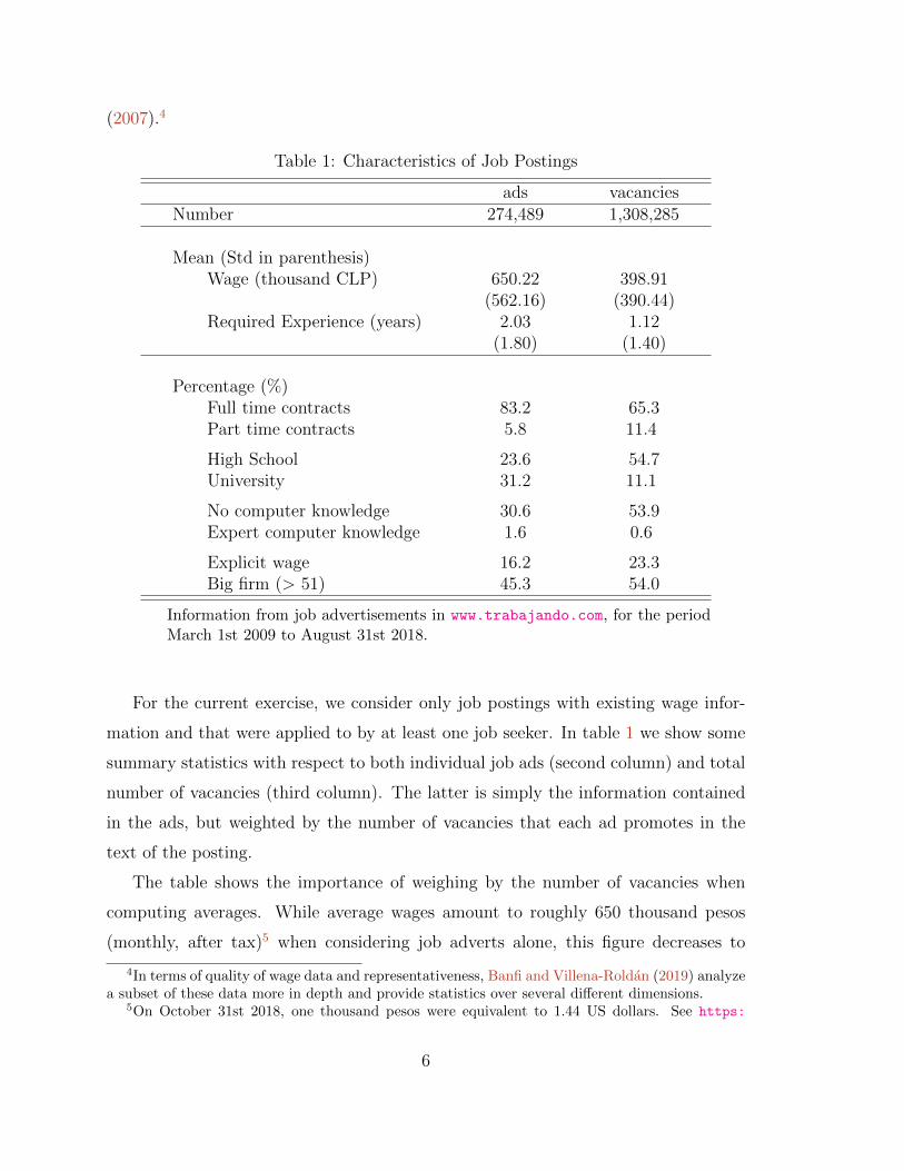
Table 1: Characteristics of Job Postings

ads vacanciesNumber 274,489 1,308,285

Mean (Std in parenthesis)Wage (thousand CLP) 650.22 398.91

(562.16) (390.44)Required Experience (years) 2.03 1.12

(1.80) (1.40)

Percentage (%)Full time contracts 83.2 65.3Part time contracts 5.8 11.4

High School 23.6 54.7University 31.2 11.1

No computer knowledge 30.6 53.9Expert computer knowledge 1.6 0.6

Explicit wage 16.2 23.3Big firm (> 51) 45.3 54.0

Information from job advertisements in www.trabajando.com, for the periodMarch 1st 2009 to August 31st 2018.

For the current exercise, we consider only job postings with existing wage infor-

mation and that were applied to by at least one job seeker. In table 1 we show some

summary statistics with respect to both individual job ads (second column) and total

number of vacancies (third column). The latter is simply the information contained

in the ads, but weighted by the number of vacancies that each ad promotes in the

text of the posting.

The table shows the importance of weighing by the number of vacancies when

computing averages. While average wages amount to roughly 650 thousand pesos

(monthly, after tax)5 when considering job adverts alone, this figure decreases to

4In terms of quality of wage data and representativeness, Banfi and Villena-Roldan (2019) analyzea subset of these data more in depth and provide statistics over several different dimensions.

5On October 31st 2018, one thousand pesos were equivalent to 1.44 US dollars. See https:

6

around 398 thousand pesos when we take into account how many actual jobs the first

figure represents. One direct implication from this, is that lower paying jobs in the

website tend to advertise a higher number of positions. According to the Chilean

National Statistics Institute,6 the median after tax wage in Chile during 2014 (mid

point of our sample) was 305 thousand pesos.

In the rest of the table, we also display average required experience (in years),

as well as the fraction of job positions with particular requirements (e.g., education)

or offering certain characteristics (e.g., full/part time contracts). All results in what

follows are weighted by the number of vacancies to better represent the actual job

creation flow generated by the website.

0.5

11.

52

2.5

Den

sity

11 12 13 14 15 16Log wages

Above HP-U Below HP-U

.06

.08

.1.1

2 U

nem

ploy

men

t

2009m3 2010m9 2012m3 2013m9 2015m3 2016m9 2018m3

Unemployment rateHodrick Prescott trend

Figure 1: Histogram of log wages, according to the aggregate unemployment rate at the time

of posting (left) and time series of unemployment rate and its Hodrick-Prescott smoothed trend

(right).

In the left panel of figure 1 we plot histograms for log wages (unweighted) of job

ads during our sample period. In the figure we split the sample according to the

national unemployment rate in the Chilean economy during the month in which each

particular ad was posted: in gray, we show log wages of vacancies posted when the

unemployment rate was above its trend (computed using a standard Hodrick-Prescott

filter), while in blue we show the case when it was below.7 As seen from the figure,

there is a clear shift towards higher wages during periods of low unemployment. The

//www.xe.com/currencycharts/?from=CLP&to=USD&view=5Y.6See https://www.ine.cl/estadisticas/ingresos-y-gastos/esi7For reference, the Chilean unemployment rate during the time period considered was on average

6.8%, fluctuating between 5.7% and 11.6%.

7

right panel in the same figure shows the aggregate unemployment rate in the Chilean

economy during our sample period, along a Hodrick-Prescott trend. From the figure

we can see a decline in unemployment due to recovery of the economy following the

global mortgage crisis of 2008-2009. After the mid part of 2015, the figure shows a

small increase in the unemployment rate.

The data of www.trabajando.com is quite representative of the Chilean labor

market between 2010 and 2018. Since ad wages in this website are associated with

job creation in the short term, we need to compare them to the wages of jobs actually

created in the economy around the publication dates of the ads.

To show the representativeness of the website, we compare it with the nation-

ally representative survey Encuesta Suplementaria de Ingresos (ESI), which measures

salaries and characteristics of recently hired workers in the Chilean economy. This

survey has questions about wages for interviewees of the National Employment Survey

of the Instituto Nacional de Estadısticas during October, November, and December

of each year. The survey is similar to the Outgoing Rotation Group of the Current

Population Survey (CPS-ORG) in the US, but each household stays in the sample

for six consecutive quarters.8

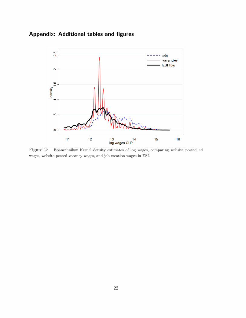
As noted above, to make the website and ESI flow data comparable, we weigh ad

data in www.trabajando.com by the number of vacancies at each posting. We make

a simple comparison between posted wages from our data with wages declared by

those recently hired in the ESI. Note that this is a simplification, given that there is

no guarantee that posted and realized wages are the same for a given match, because

of wage bargaining or ex post compensations. The job ad wage distribution from our

dataset has a greater average than the other two distributions, while the vacancy-

adjusted and the ESI job flow distributions are very similar, despite some bunching

near “round” wage numbers (e.g., 250, 500, etc. thousand CLP). Figure 2 in the

appendix depicts density estimators of log-wage distributions.

To compare job composition in terms of educational levels, we further assume that

8Data are available in https://www.ine.cl/estadisticas/sociales/ingresos-y-gastos/

encuesta-suplementaria-de-ingresos. We report data on the declared monthly wage at themain job. The 2018 survey only has household heads information. Nevertheless, the results wereport barely change if we exclude the 2018 data from the sample.

8

employers requiring a specific educational level in their ads end up hiring workers

matching those requirements.9 In terms of educational levels, there are two alter-

native high school tracks in Chile: the Scientific-Humanities (SH) track, aimed at

students planning to attend university, and the Technical-Professional (TP) track,

aimed at individuals targeting the labor market or wishing to pursue a technical de-

gree. At the tertiary level, there is university education (4 to 6 year undergraduate

degrees) as well as a Technical Professional tertiary (2 to 3 year degrees). Demand for

graduate degrees is small partly due to the fact that many degrees such as lawyers,

physicians, and engineers are granted as undergraduate university degrees. As for

industry comparisons, we assume that firms in www.trabajando.com create jobs in

the industry they belong to, which we characterize using a one-digit (aggregate) code.

The educational attainment of new hirings (ESI) roughly matches the distribu-

tion of educational requirements for workers (www.trabajando.com) with at least

high school education: the website data apparently misses job creation for very low-

educated workers, even though the educational level of the realized hiring is unob-

served. The ESI flow contains 38% of workers with less than high school education,

while only 11% of vacancy postings require primary or no specific educational level.

Table 5 shows these results in the appendix.

In terms of industry, we show in table 6 in the appendix that the shares of in-

dustries (at the 1 digit level) align well across datasets. Again, in the website we

measure the fraction of job vacancies from firms in the different sectors, while in the

ESI we compute the fraction of new hires in each of the same sectors. The caveat

here is that agriculture, silviculture, construction and public administration jobs are

excluded. The correlation of industry shares between website vacancies and survey

data, once we omit these sectors, is as high as 0.74.

9Although we do not have hiring records, there is evidence showing that job seekers apply to jobsoffering wages aligned to their own expectations, and tend to comply to requirements: see Banfiet al. (2018a) and Banfi et al. (2018b).

9

3 Methodology

Our analysis is based on estimating linear regressions relating the log offered wage wa

(for job a) with the aggregate unemployment rate at the time of its posting, Ut(a) and

a set of covariates describing the job, Xa. More specifically, the baseline regression

we estimate is

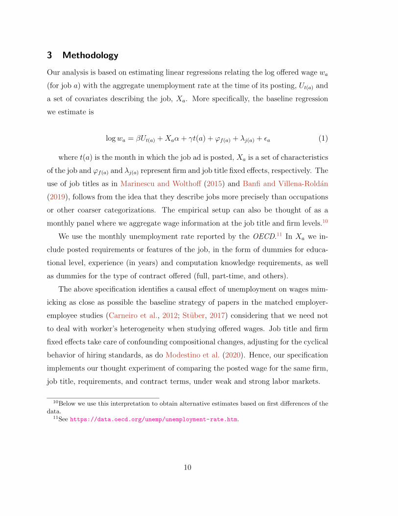
logwa = βUt(a) +Xaα + γt(a) + ϕf(a) + λj(a) + εa (1)

where t(a) is the month in which the job ad is posted, Xa is a set of characteristics

of the job and ϕf(a) and λj(a) represent firm and job title fixed effects, respectively. The

use of job titles as in Marinescu and Wolthoff (2015) and Banfi and Villena-Roldan

(2019), follows from the idea that they describe jobs more precisely than occupations

or other coarser categorizations. The empirical setup can also be thought of as a

monthly panel where we aggregate wage information at the job title and firm levels.10

We use the monthly unemployment rate reported by the OECD.11 In Xa we in-

clude posted requirements or features of the job, in the form of dummies for educa-

tional level, experience (in years) and computation knowledge requirements, as well

as dummies for the type of contract offered (full, part-time, and others).

The above specification identifies a causal effect of unemployment on wages mim-

icking as close as possible the baseline strategy of papers in the matched employer-

employee studies (Carneiro et al., 2012; Stuber, 2017) considering that we need not

to deal with worker’s heterogeneity when studying offered wages. Job title and firm

fixed effects take care of confounding compositional changes, adjusting for the cyclical

behavior of hiring standards, as do Modestino et al. (2020). Hence, our specification

implements our thought experiment of comparing the posted wage for the same firm,

job title, requirements, and contract terms, under weak and strong labor markets.

10Below we use this interpretation to obtain alternative estimates based on first differences of thedata.

11See https://data.oecd.org/unemp/unemployment-rate.htm.

10

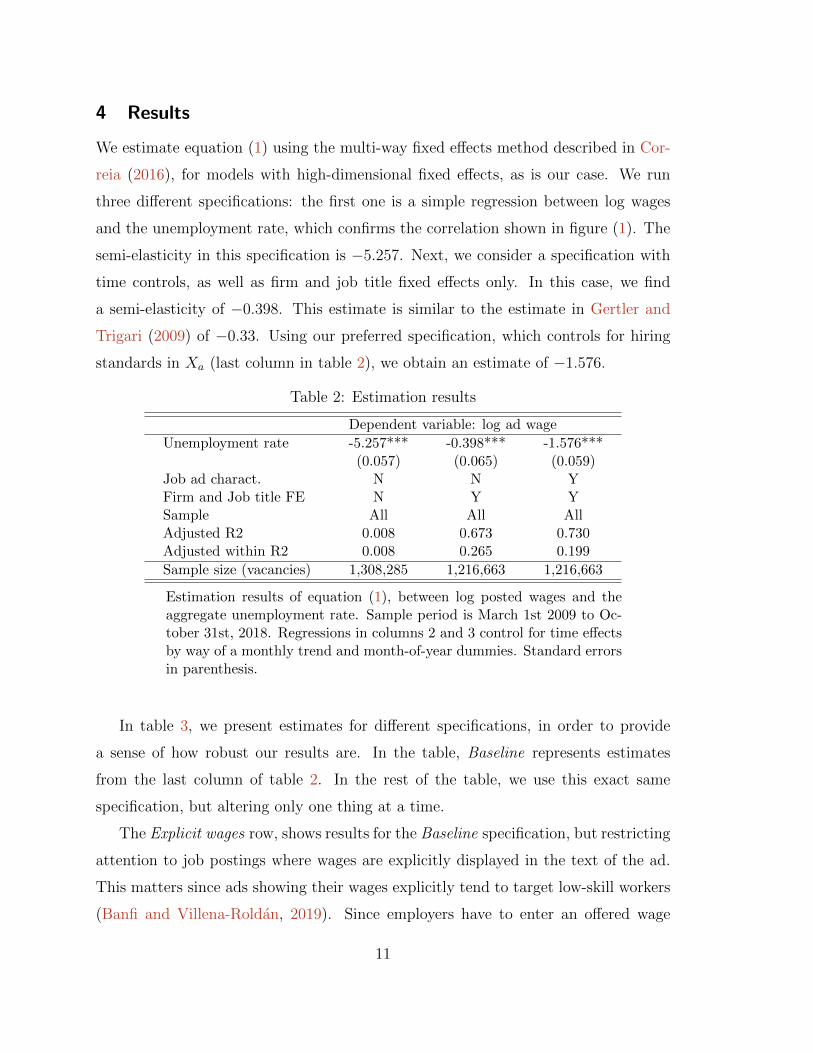
4 Results

We estimate equation (1) using the multi-way fixed effects method described in Cor-

reia (2016), for models with high-dimensional fixed effects, as is our case. We run

three different specifications: the first one is a simple regression between log wages

and the unemployment rate, which confirms the correlation shown in figure (1). The

semi-elasticity in this specification is −5.257. Next, we consider a specification with

time controls, as well as firm and job title fixed effects only. In this case, we find

a semi-elasticity of −0.398. This estimate is similar to the estimate in Gertler and

Trigari (2009) of −0.33. Using our preferred specification, which controls for hiring

standards in Xa (last column in table 2), we obtain an estimate of −1.576.

Table 2: Estimation results

Dependent variable: log ad wage

Unemployment rate -5.257*** -0.398*** -1.576***(0.057) (0.065) (0.059)

Job ad charact. N N YFirm and Job title FE N Y YSample All All AllAdjusted R2 0.008 0.673 0.730Adjusted within R2 0.008 0.265 0.199

Sample size (vacancies) 1,308,285 1,216,663 1,216,663

Estimation results of equation (1), between log posted wages and theaggregate unemployment rate. Sample period is March 1st 2009 to Oc-tober 31st, 2018. Regressions in columns 2 and 3 control for time effectsby way of a monthly trend and month-of-year dummies. Standard errorsin parenthesis.

In table 3, we present estimates for different specifications, in order to provide

a sense of how robust our results are. In the table, Baseline represents estimates

from the last column of table 2. In the rest of the table, we use this exact same

specification, but altering only one thing at a time.

The Explicit wages row, shows results for the Baseline specification, but restricting

attention to job postings where wages are explicitly displayed in the text of the ad.

This matters since ads showing their wages explicitly tend to target low-skill workers

(Banfi and Villena-Roldan, 2019). Since employers have to enter an offered wage

11

even if they choose not to post them in www.trabajando.com, we can assess whether

showing wages makes a difference in terms of cyclicality. Since 75-85% of job ads hide

wages in most websites12, we have an opportunity to check that wage explicitness does

not matter much for ad wage cyclicality: the estimate for this case is very similar to

our baseline.

The No Firm FE and No Job Title FE rows represent the estimation of equation

(1) when we remove firm and job title fixed effects, respectively. Since dropping firm

fixed effects reduces procyclicality of wages, this suggests a cyclical change of firm

composition. In contrast, the estimate without job title fixed effects is very similar

to the baseline, suggesting that the job title cyclical variation is nearly captured as a

compositional change in employers posting ads with particular job titles.

The results when we do not weight job advertisement by the number of vacancies

in the ad are in row No weights. We notice the absence of weights reduces wage

procyclicality because the number of vacancies per ad is procyclical as well. Hence,

it is possible that estimates using other databases without vacancy information un-

derestimate wage procyclicality.

The row Likely UE considers job postings where more than 90% of applicants

are unemployed at the time of their application to the position. In line with Gertler

et al. (2016), new jobs filled by unemployed workers are less procyclical than hirings

originated in job-to-job transitions. This also aligns with the literature surveyed by

Pissarides (2009) showing that job movers drive a great deal of wage growth.

When we consider the interaction between job title and firm identifier as our

definition of a job, as in Hazell and Taska (2019), we can estimate our baseline

specification in differences (and thus, without time trends) which leads to results in

row Baseline (diffs). The main takeaway from all these different estimations is that

the negative (and significant) semi-elasticity remains.

The last two rows of table 3 show results from performing a simple test of asymme-

tries in the effect of aggregate unemployment on log-wages. To obtain these numbers,

we run our baseline equation but add an interaction term between the unemployment

rate and a dummy variable for the case in which its value is above its long run trend,

12See for instance Kuhn and Shen (2013); Marinescu and Wolthoff (2015); Hazell and Taska (2019)

12

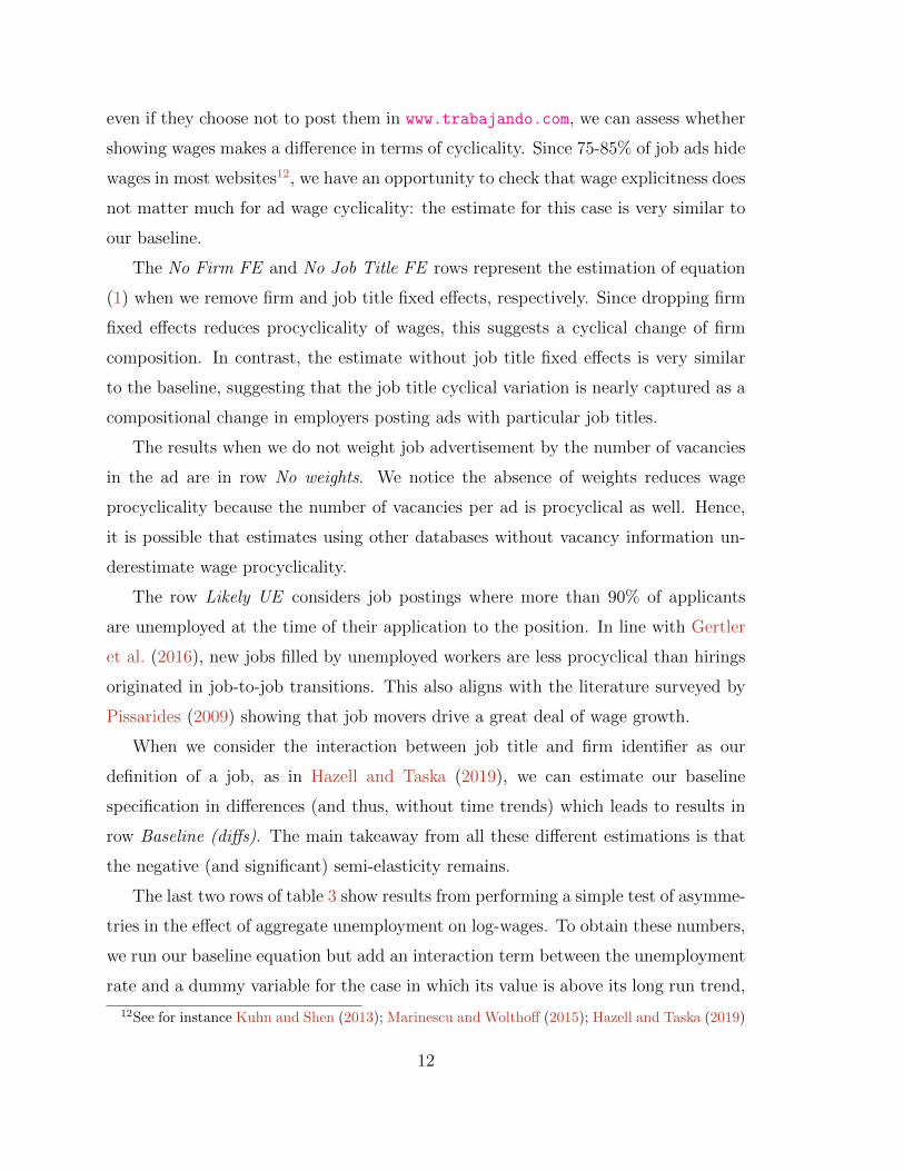
as computed using a standard Hodrick-Prescott (HP) filter. In the table we observe

that when unemployment is above the HP trend, the estimated cyclicality of wages is

below our baseline estimates (−1.136 vs −1.576) while when unemployment levels are

low, the cyclicality is significantly higher (estimate of −4.696). These results show

that when unemployment is high, wages are relatively more “sticky”, in the sense

that they do not react as strongly to unemployment as when unemployment is low.

While this asymmetry is also found by Hazell and Taska (2019), even in the U above

trend scenario, the semi-elasticity estimate is still on the high side of the estimates

in the literature.

Table 3: Estimation results: Robustness

estimate std. err. adj. R2 within R2 Sample Size

BASELINE -1.576 (0.059) 0.730 0.199 1, 216, 663Explicit ads -1.694 (0.135) 0.732 0.200 291, 900No Firm FE -0.793 (0.048) 0.634 0.282 1, 221, 212No Job Title FE -1.657 (0.061) 0.677 0.322 1, 216, 663No weights -0.565 (0.116) 0.721 0.222 251, 882Likely UE -0.852 (0.089) 0.721 0.171 620, 145Baseline (diffs) -2.835 (0.511) 0.088 – 91, 069U above trend -1.136 (0.049) 0.731 0.199 1, 216, 663U below trend -4.696 (0.049) 0.731 0.199 1, 216, 663

Estimation results for alternative specifications. Sample period is March 1st 2009 toOctober 31st 2018. All regressions control for time effects by way of a monthly trendand month-of-year dummies to control for seasonality.

A caveat on our results: it is a widely extended practice to post net monthly wages

in job ads in Chile, as is to write work contracts in that fashion. As hours worked are

somewhat procyclical, monthly wages might be affected by longer hours in expansive

times. During 2010-18, ESI data shows that 44% of newly hired formal employees

usually work the maximum of 45 weekly hours (with no overtime compensation)

determined by law.

In table 7 (in the appendix) we present estimates when restricting the sample

by industry of posting firms. From the table, we can observe that the estimated

semi-elasticities are heterogeneous across sectors, with Services displaying the high-

est cyclicality while the Manufacture sector displays almost acyclical wages. An

13

interesting case is that of the Finance sector, which displays highly counter-cyclical

wages.

5 Hiring standards and wage cyclicality

Our main result from table 2 is that our estimates without job characteristic controls,

such as requirements and contract terms (in Xa) imply a lower cyclicality of wages

than when we do include them. In what follows, we use a decomposition due to

Gelbach (2016) to understand this result. In our exercise, we show that the lower

cyclicality found in the second specification of table 2 (third column of the table),

where we ignore information on job characteristics, is due to the comovement of these

with the unemployment rate.

Following the notation in Gelbach (2016), let βfull be a vector containing the set

of estimators from the full regression in equation (1), with the exception of those

related to Xa. One of these estimates corresponds to the particular coefficient for

the semi-elasticity of −1.576 in the last column of table 2. On the other hand, let

βbase be the vector containing the set of estimates from the specification with no job

characteristic controls Xa (associated to the estimate of −0.398 in table 2). Using

standard results on omitted variable bias in linear regressions, it can be shown that

βbase − βfull = (X ′1X1)−1X ′1XaβXa (2)

where X1 is a matrix containing all regressors in equation (1) with the exception of

Xa. Hence, X1 includes the unemployment rate plus all fixed effects from equation

(1). On the other hand, βXa are the coefficients related to Xa in the full specification.

Thus, this result is useful for our analysis since it states that the difference in

the point estimates related to the semi-elasticity of wages to the unemployment rate

can be decomposed linearly in terms of both the effect of job characteristics on log

wages (term βXa in the equation above) and how these characteristics interact with

the unemployment rate, i.e., their cyclicality (the rest of terms in the right-hand side

in equation 2). Since we are interested in the decomposition for the point estimate

of the semi-elasticity of wages to the unemployment rate, the procedure suggested

14

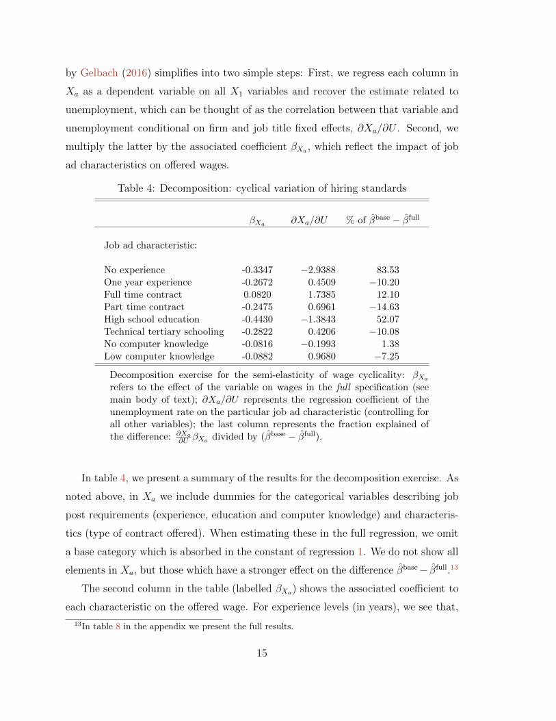
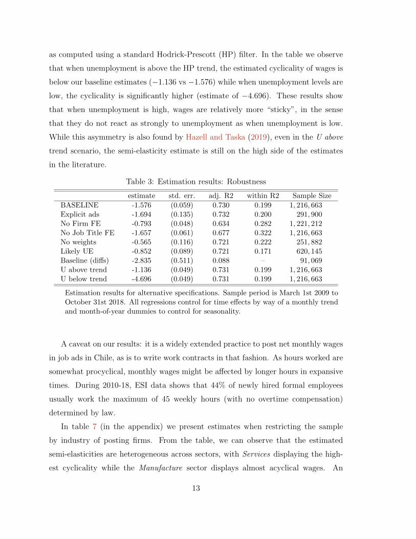
by Gelbach (2016) simplifies into two simple steps: First, we regress each column in

Xa as a dependent variable on all X1 variables and recover the estimate related to

unemployment, which can be thought of as the correlation between that variable and

unemployment conditional on firm and job title fixed effects, ∂Xa/∂U . Second, we

multiply the latter by the associated coefficient βXa , which reflect the impact of job

ad characteristics on offered wages.

Table 4: Decomposition: cyclical variation of hiring standards

βXa ∂Xa/∂U % of βbase − βfull

Job ad characteristic:

No experience -0.3347 −2.9388 83.53One year experience -0.2672 0.4509 −10.20Full time contract 0.0820 1.7385 12.10Part time contract -0.2475 0.6961 −14.63High school education -0.4430 −1.3843 52.07Technical tertiary schooling -0.2822 0.4206 −10.08No computer knowledge -0.0816 −0.1993 1.38Low computer knowledge -0.0882 0.9680 −7.25

Decomposition exercise for the semi-elasticity of wage cyclicality: βXa

refers to the effect of the variable on wages in the full specification (seemain body of text); ∂Xa/∂U represents the regression coefficient of theunemployment rate on the particular job ad characteristic (controlling forall other variables); the last column represents the fraction explained ofthe difference: ∂Xa

∂U βXa divided by (βbase − βfull).

In table 4, we present a summary of the results for the decomposition exercise. As

noted above, in Xa we include dummies for the categorical variables describing job

post requirements (experience, education and computer knowledge) and characteris-

tics (type of contract offered). When estimating these in the full regression, we omit

a base category which is absorbed in the constant of regression 1. We do not show all

elements in Xa, but those which have a stronger effect on the difference βbase− βfull.13

The second column in the table (labelled βXa) shows the associated coefficient to

each characteristic on the offered wage. For experience levels (in years), we see that,

13In table 8 in the appendix we present the full results.

15

relative to the base category (dummy for the highest level of experience dummy, or 18

years in our sample), jobs requiring either no or only one year of experience pay less

than jobs with higher requirements. In terms of offered contracts, full-time contracts

pay more while part-time contracts pay less than the base category, which is “no

contract information” in the ad. For education, the omitted category is “university

education” and, as expected, jobs requiring both high school education or a technical

tertiary diploma pay relatively less. Finally, for computer knowledge, we see from the

table that jobs requiring low or no computer knowledge pay less than the omitted

related category (”expert knowledge”).

The third column in table 4, labelled ∂Xa/∂U , shows how job characteristics

change when aggregate unemployment changes. For each sub-group of characteristics

(experience, education, contract type and computer knowledge) we see that increases

in the unemployment rate lead to hiring standards to be risen and viceversa. This

can be seen for example, in the two considered categories of required experience: the

correlation between “no experience” jobs and unemployment is negative, while it is

positive for “one year experience” jobs and unemployment. In other words, rising

unemployment is associated to periods of time when jobs increase hiring standards

for prospective applicants, and to times when employers reduce the quality of jobs

offered in attributes other than wages. These findings are very similar to those by

Modestino et al. (2016, 2020).

The last column in table 4 shows the relative importance of each particular char-

acteristic in the table to explain the difference in estimates (base minus full). Given

the results in Gelbach (2016) and equation (2), the last column is simply the ra-

tio between the product of the terms in the second and third column, divided by

βbase− βfull. From the table we see that “no experience” and “high school” education

requirements are the ones that explain the most of the difference.

These results are evidence of countercyclical hiring standards. In an economic

downturn, employers adjust in two ways. First, for a given job position, they pay

less for a given set of attributes embedded in a worker profile. Second, they raise the

bar regarding the type of attribute requirements for prospective applicants. Hence,

in downturns employers intend to hire workers of better qualifications for a lower

16

wage to do the same job and this leads to our main conclusion: not accounting for

countercyclical upgrade of requirements leads to underestimating the true cyclicality

of wages.

6 Conclusions

In this paper we use internet data on posted wages to study cyclicality of wages at

new positions. Our setup provides at least two advantages over previous literature:

First, we can study how wage offers evolve over the cycle, without worrying about

cyclical mismatch patterns that may occur when the applicant, firm or job composi-

tion changes, avoiding problems due to the cyclical upgrade, as remarked by Gertler

and Trigari (2009). Second, the fact that we observed offered instead of realized wages

allows us to minimize concerns about cyclical mismatch. Third, we show that job

requirements associated with higher wages move countercyclically, as do Modestino

et al. (2020). The latter is relevant since omitting fluctuating hiring standards af-

fects the estimation of wage cyclicality, even if one focuses in a narrowly defined job

title. Employers ask for more education or more experience to fill the vacancies in a

downturn, effectively widening the gap between the offered wage and a counterfactual

wage that a more educated or experienced worker would obtained in a neutral cyclical

situation.

These results enrich the view of the hiring process beyond the role of wage stick-

iness as a major driver of the cyclical behavior of the labor market. Our treatment

of the evidence shows the inevitable interlink between offered wages and job ad re-

quirements. Although some models try to explain these facts (Baydur, 2017; Carrillo-

Tudela et al., 2018), more theoretical research needs to shade light on the facts we

uncover here to gain understanding of the cyclical behavior of wages and worker flows.

17

References

Albagli, E., G. Contreras, M. Tapia, and J. M. Wlasiuk (2017). Wage Cyclicality of

New and Continuing Jobs: Evidence from Chilean Tax Records. Working paper,

Central Bank of Chile.

Banfi, S., S. Choi, and B. Villena-Roldan (2018a). Deconstructing Job Search Behav-

ior. Technical report. Working Paper 343, Center for Applied Economics, University

of Chile.

Banfi, S., S. Choi, and B. Villena-Roldan (2018b). Sorting on-line and on-time.

Technical report. Working Paper 336, Center for Applied Economics, University of

Chile.

Banfi, S. and B. Villena-Roldan (2019). Do High-Wage Jobs Attract More Appli-

cants? Directed Search Evidence from the Online Labor Market. Journal of Labor

Economics 37 (3), 715–746.

Baydur, I. (2017). Worker Selection, Hiring, and Vacancies. American Economic

Journal: Macroeconomics 9 (1), 88–127.

Brencic, V. (2012). Wage Posting: Evidence from Job Ads. Canadian Journal of

Economics/Revue canadienne d’economique 45 (4), 1529–1559.

Carneiro, A., P. Guimaraes, and P. Portugal (2012). Real Wages and the Business

Cycle: Accounting for Worker, Firm, and Job Title Heterogeneity. American Eco-

nomic Journal: Macroeconomics 4 (2), 133–52.

Carrillo-Tudela, C., H. Gartner, and L. Kaas (2018). Understanding Vacancy Yields:

Evidence from German Data. Mimeo.

Correia, S. (2016). Linear Models with High-Dimensional Fixed Effects: An Efficient

and Feasible Estimator. Technical report. Working Paper.

18

Costain, J. S. and M. Reiter (2008). Business Cycles, Unemployment Insurance,

and the Calibration of Matching Models. Journal of Economic Dynamics and

Control 32 (4), 1120–1155.

Dapi, B. (2019). Wage Cyclicality and Composition Bias in the Norwegian Economy.

Forthcoming, Scandinavian Journal of Economics .

Gelbach, J. B. (2016). When Do Covariates Matter? And Which Ones, and How

Much? Journal of Labor Economics 34 (2), 509–543.

Gertler, M., C. Huckfeldt, and A. Trigari (2016). Unemployment Fluctuations, Match

Quality, and the Wage Cyclicality of New Hires. Working Paper 22341, National

Bureau of Economic Research. Forthcoming, Review of Economic Studies.

Gertler, M. and A. Trigari (2009). Unemployment Fluctuations with Staggered Nash

Wage Bargaining. Journal of Political Economy 117 (1), 38–86.

Haefke, C., M. Sonntag, and T. Van Rens (2013). Wage Rigidity and Job Creation.

Journal of Monetary Economics 60 (8), 887–899.

Hagedorn, M. and I. Manovskii (2008). The Cyclical Behavior of Equilibrium Unem-

ployment and Vacancies Revisited. American Economic Review 98 (4), 1692–1706.

Hall, R. (2005). Employment Fluctuations with Equilibrium Wage Stickiness. Amer-

ican Economic Review 95 (1), 50–65.

Hazell, J. and B. Taska (2019). Downward Rigidity in the Wage for New Hires.

Mimeo, MIT Economics Department.

Kuhn, P. and K. Shen (2013). Gender Discrimination in Job Ads: Evidence from

China. The Quarterly Journal of Economics 128 (1), 287–336.

Marinescu, I. E. and R. P. Wolthoff (2015). Opening the Black Box of the Matching

Function: The Power of Words. Discussion Paper 9071, IZA. Forthcoming, Journal

of Labor Economics.

19

Martins, P. S., G. Solon, and J. P. Thomas (2012). Measuring What Employers Do

about Entry Wages over the Business Cycle: A New Approach. American Economic

Journal: Macroeconomics 4 (4), 36–55.

McGregor, A. (1978). Unemployment Duration and Re-employment probability. The

Economic Journal 88 (352), 693–706.

Modestino, A. S., D. Shoag, and J. Ballance (2016). Downskilling: Changes in Em-

ployer Skill Requirements over the Business Cycle. Labour Economics 41, 333 –

347. SOLE/EALE conference issue 2015.

Modestino, A. S., D. Shoag, and J. Ballance (2020). Upskilling: Do employers demand

greater skill when workers are plentiful? Forthcoming, The Review of Economics

and Statistics .

Oreopoulos, P., T. Von Wachter, and A. Heisz (2012). The Short-and Long-Term

Career Effects of Graduating in a Recession. American Economic Journal: Applied

Economics 4 (1), 1–29.

Pissarides, C. A. (2009). The Unemployment Volatility Puzzle: Is Wage Stickiness

the Answer? Econometrica 77 (5), 1339–1369.

Reder, M. W. (1964). Wage Structure and Structural Unemployment. The Review of

Economic Studies 31 (4), 309–322.

Sahin, A., J. Song, G. Topa, and G. L. Violante (2014). Mismatch Unemployment.

American Economic Review 104 (11), 3529–3564.

Sedlacek, P. (2014). Match Efficiency and Firms’ Hiring Standards. Journal of Mon-

etary Economics 62, 123–133.

Shimer, R. (2005). The Cyclical Behavior of Equilibrium Unemployment and Vacan-

cies. American Economic Review 95 (1), 25–49.

Shimer, R. (2010). Labor Markets and Business Cycles. CREI Lectures in Macroe-

conomics. Princeton University Press.

20

Stuber, H. (2017). The Real Wage Cyclicality of Newly Hired and Incumbent Workers

in Germany. The Economic Journal 127 (600), 522–546.

Swanson, E. T. (2007). Real Wage Cyclicality in the Panel Study of Income Dynamics.

Scottish Journal of Political Economy 54 (5), 617–647.

21

Appendix: Additional tables and figures

Figure 2: Epanechnikov Kernel density estimates of log wages, comparing website posted ad

wages, website posted vacancy wages, and job creation wages in ESI.

22

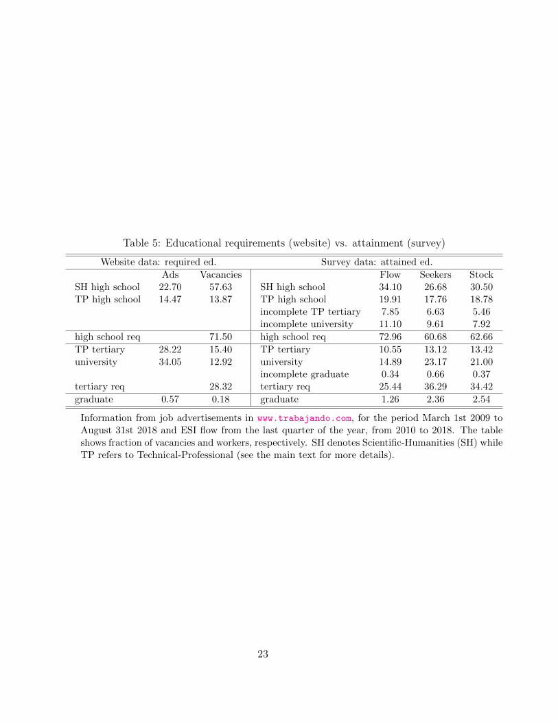
Table 5: Educational requirements (website) vs. attainment (survey)

Website data: required ed. Survey data: attained ed.

Ads Vacancies Flow Seekers StockSH high school 22.70 57.63 SH high school 34.10 26.68 30.50TP high school 14.47 13.87 TP high school 19.91 17.76 18.78

incomplete TP tertiary 7.85 6.63 5.46incomplete university 11.10 9.61 7.92

high school req 71.50 high school req 72.96 60.68 62.66

TP tertiary 28.22 15.40 TP tertiary 10.55 13.12 13.42university 34.05 12.92 university 14.89 23.17 21.00

incomplete graduate 0.34 0.66 0.37tertiary req 28.32 tertiary req 25.44 36.29 34.42

graduate 0.57 0.18 graduate 1.26 2.36 2.54

Information from job advertisements in www.trabajando.com, for the period March 1st 2009 toAugust 31st 2018 and ESI flow from the last quarter of the year, from 2010 to 2018. The tableshows fraction of vacancies and workers, respectively. SH denotes Scientific-Humanities (SH) whileTP refers to Technical-Professional (see the main text for more details).

23

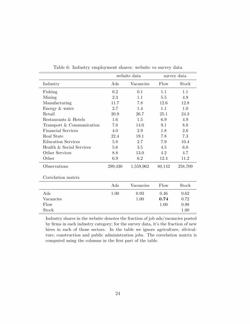
Table 6: Industry employment shares: website vs survey data

website data survey data

Industry Ads Vacancies Flow Stock

Fishing 0.2 0.1 1.1 1.1Mining 2.3 1.1 5.5 4.9Manufacturing 11.7 7.8 12.6 12.8Energy & water 2.7 1.4 1.1 1.0Retail 20.9 26.7 25.1 24.3Restaurants & Hotels 1.6 1.5 6.9 4.9Transport & Communication 7.0 14.0 9.1 8.8Financial Services 4.0 2.9 1.8 2.6Real State 22.4 19.1 7.8 7.3Education Services 5.8 2.7 7.9 10.4Health & Social Services 5.6 3.5 4.5 6.0Other Services 8.8 13.0 4.2 4.7Other 6.9 6.2 12.4 11.2

Observations 299,430 1,559,962 80,142 258,709

Correlation matrix

Ads Vacancies Flow Stock

Ads 1.00 0.93 0.46 0.62Vacancies 1.00 0.74 0.72Flow 1.00 0.98Stock 1.00

Industry shares in the website denotes the fraction of job ads/vacancies postedby firms in each industry category; for the survey data, it’s the fraction of newhires in each of those sectors. In the table we ignore agriculture, silvicul-ture, construction and public administration jobs. The correlation matrix iscomputed using the columns in the first part of the table.

24

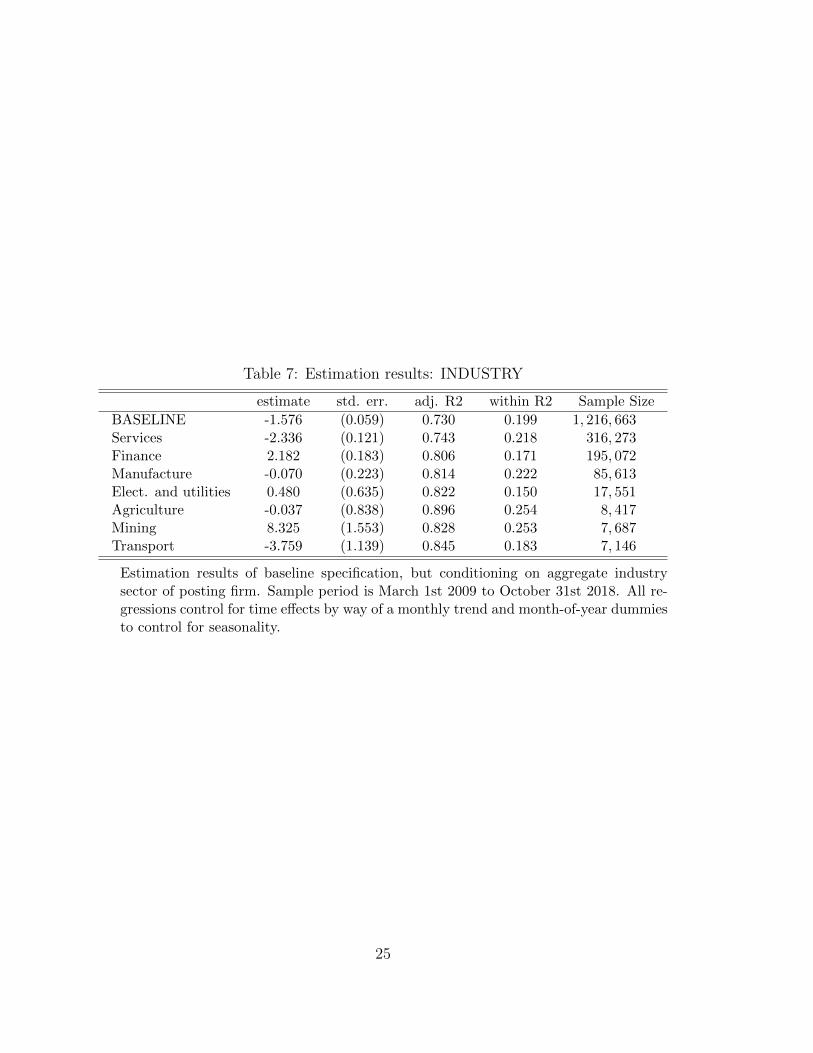
Table 7: Estimation results: INDUSTRY

estimate std. err. adj. R2 within R2 Sample Size

BASELINE -1.576 (0.059) 0.730 0.199 1, 216, 663Services -2.336 (0.121) 0.743 0.218 316, 273Finance 2.182 (0.183) 0.806 0.171 195, 072Manufacture -0.070 (0.223) 0.814 0.222 85, 613Elect. and utilities 0.480 (0.635) 0.822 0.150 17, 551Agriculture -0.037 (0.838) 0.896 0.254 8, 417Mining 8.325 (1.553) 0.828 0.253 7, 687Transport -3.759 (1.139) 0.845 0.183 7, 146

Estimation results of baseline specification, but conditioning on aggregate industrysector of posting firm. Sample period is March 1st 2009 to October 31st 2018. All re-gressions control for time effects by way of a monthly trend and month-of-year dummiesto control for seasonality.

25

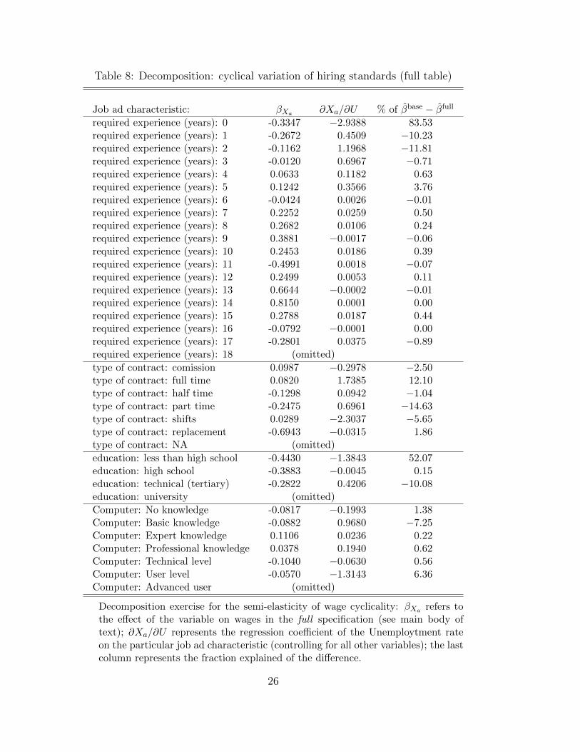
Table 8: Decomposition: cyclical variation of hiring standards (full table)

Job ad characteristic: βXa ∂Xa/∂U % of βbase − βfull

required experience (years): 0 -0.3347 −2.9388 83.53required experience (years): 1 -0.2672 0.4509 −10.23required experience (years): 2 -0.1162 1.1968 −11.81required experience (years): 3 -0.0120 0.6967 −0.71required experience (years): 4 0.0633 0.1182 0.63required experience (years): 5 0.1242 0.3566 3.76required experience (years): 6 -0.0424 0.0026 −0.01required experience (years): 7 0.2252 0.0259 0.50required experience (years): 8 0.2682 0.0106 0.24required experience (years): 9 0.3881 −0.0017 −0.06required experience (years): 10 0.2453 0.0186 0.39required experience (years): 11 -0.4991 0.0018 −0.07required experience (years): 12 0.2499 0.0053 0.11required experience (years): 13 0.6644 −0.0002 −0.01required experience (years): 14 0.8150 0.0001 0.00required experience (years): 15 0.2788 0.0187 0.44required experience (years): 16 -0.0792 −0.0001 0.00required experience (years): 17 -0.2801 0.0375 −0.89required experience (years): 18 (omitted)

type of contract: comission 0.0987 −0.2978 −2.50type of contract: full time 0.0820 1.7385 12.10type of contract: half time -0.1298 0.0942 −1.04type of contract: part time -0.2475 0.6961 −14.63type of contract: shifts 0.0289 −2.3037 −5.65type of contract: replacement -0.6943 −0.0315 1.86type of contract: NA (omitted)

education: less than high school -0.4430 −1.3843 52.07education: high school -0.3883 −0.0045 0.15education: technical (tertiary) -0.2822 0.4206 −10.08education: university (omitted)

Computer: No knowledge -0.0817 −0.1993 1.38Computer: Basic knowledge -0.0882 0.9680 −7.25Computer: Expert knowledge 0.1106 0.0236 0.22Computer: Professional knowledge 0.0378 0.1940 0.62Computer: Technical level -0.1040 −0.0630 0.56Computer: User level -0.0570 −1.3143 6.36Computer: Advanced user (omitted)

Decomposition exercise for the semi-elasticity of wage cyclicality: βXa refers tothe effect of the variable on wages in the full specification (see main body oftext); ∂Xa/∂U represents the regression coefficient of the Unemploytment rateon the particular job ad characteristic (controlling for all other variables); the lastcolumn represents the fraction explained of the difference.

26