vswg, genève, 6 july 2005 1 frequency analysis mapping on unusual samplings --- f. mignard oca/...

VSWG, Genève, 6 July 20051

Frequency Analysis Mapping On Unusual Samplings

---

F. Mignard

OCA/ Cassiopée

FAMOUS


Summary Summary

• Statement of the problem

• Objectives and principles of Famous

• Performances

• Application to variable stars

• Conclusions


Times Series Times Series

• Times series are ubiquitous in observational science

– astronomy, geophysics, meteorology, oceanography

– sociology, demography

– economy and finance

• They are analysed to find synthetic description

– trends, periodic pattern, quasi-periodic signatures

• Fourier analysis has been a standard tool for many years

– well adapted to regularly sampled signal

– but plagued with aliasing effect


Regular SamplingRegular Sampling

• Problems with regular samplings

– periodic structure in the frequency space

• aliasing

• infinitely many replica of a spectral line

• assumption needed to lift the degeneracy

• Advantages of regular sampling

– no spurious lines outside the true lines

– <exp i2t, exp i2't> ~ 0 if ' k/ :: orthogonality

condition

– with one spectrum one can have all the spectral

information


Irregular SamplingIrregular Sampling

• No definition of what 'irregular' means

– continuous pattern from fully regular to fully irregular

– random sampling is much better than 'structured irregular'

• Problems with irregular samplings

– many ghost lines linked to the true lines

– <exp i2t, exp i2't> 0 for many pairs (' )

• lack of orthogonality condition

– with one spectrum one cannot extract the full spectral

information

• Advantages of irregular samplings

– no periodic structure in the frequency space

• each spectral line appears once over a large frequency range

• in principle no assumption needed to find the correct line


FAMOUS : Background and overviewFAMOUS : Background and overview

• FAMOUS makes the decomposition of a time series as :

nktstcct kkkk ,,1),2sin()2cos()( 0

• ck and sk are constant or time polynomials

• The frequencies k are also solved for

• The spectral lines are orthogonal on the sampling (as much as possible)

• FAMOUS never uses a FFT

• It can be used for any kind of time sampling

• It has a built-in system to determine the best sampling in frequency

• It detects uniform sampling and goes into dedicated procedures

• It can search for periodic functions with k = k1

• It estimates the level of significance of the periods and amplitudes

• It generates a detailed output + all the power spectrums and residuals


Application to Gaia on-board timeApplication to Gaia on-board time

1 365.26401 1664.74 267.373 sidereal year n_3

2 177.56628 121.74 268.988 lissajous period

3 398.88244 22.63 212.608 synodic jupiter n_3-n_5

4 182.62961 13.83 264.895 six months 2n_3

5 4333.41190 4.76 238.922 sideral jupiter n_5

6 378.09968 4.63 18.412 synodic saturn n_3-n_6

7 10751.37900 2.28 349.510 sideral saturn n_6

8 345.55283 1.33 272.311 synodic lissajous -n_3

9 291.95491 1.28 76.969 2*synodic venus 2*(n_2-n_3)

10 583.94321 1.13 82.919 synodic venus n_2-n_3

11 439.32954 1.01 250.119 n_3-2*n_5

12 199.44473 0.80 157.509 2 synodic jupiter 2*(n_3-n_5)

13 119.48292 0.70 266.316 sun+lissajous + n_3

14 1454.84510 0.62 246.329 2*n_2-3*n_3

15 369.65100 0.49 192.786 synodic Uranus n_3-n_7

16 367.47181 0.46 224.343 synodic Neptune n_3-n_8

period amplitude phase d µs °


Standard model for FAMOUSStandard model for FAMOUS

When k frequencies have been identified one has the model :

k

iiii tstcct1

000 )2sin()2cos()(

ppiiiii

ppiiiii

tbtbtbbS

tatataaC

2210

2210

constants or polynomial of time :

: are ,,, and ,,, 1010 kk sssccc where

where p = p(i) : degree selected for each frequency


Solution with k frequenciesSolution with k frequencies

When k frequencies have been identified one has the model :

2)()(minfit squares-leastbest ::),,( ttSba i

ri

ri

Solved in two steps :

- SVD with i = 0i and

- Levenberg-Marquardt minimisation with all the unknowns

This is a non-linear least-squares very sensitive to the starting values

Result : best decomposition of S(t) on the model with k frequencies


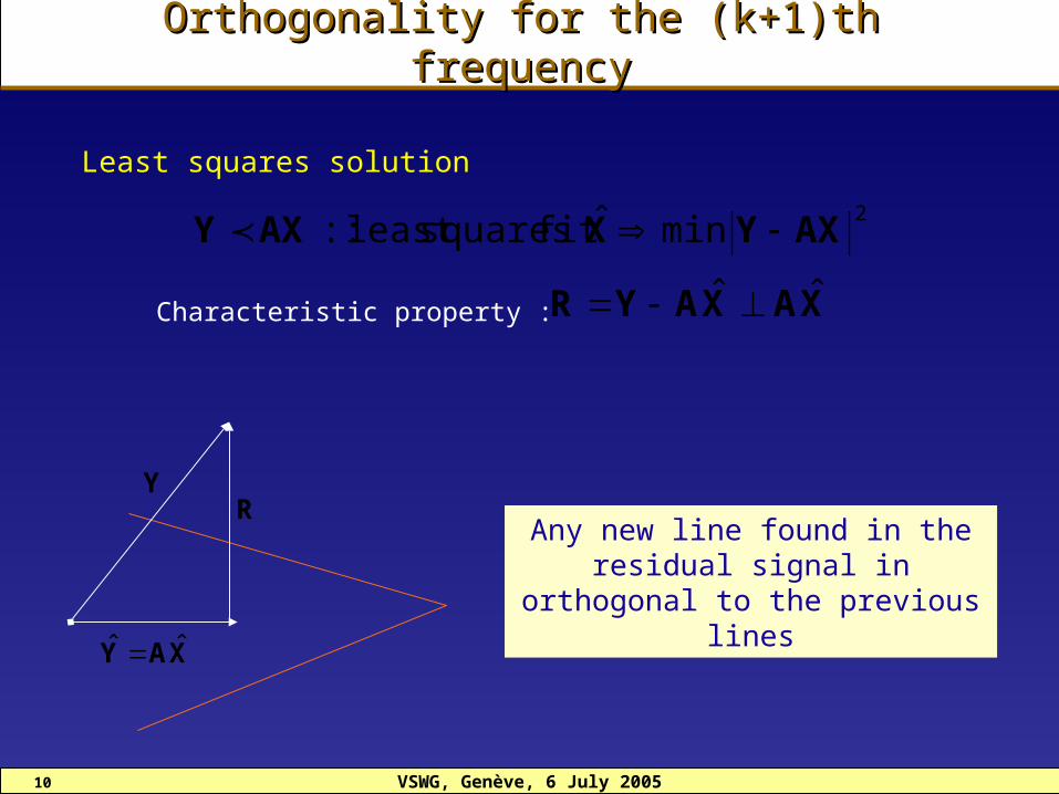
Orthogonality for the (k+1)th frequencyOrthogonality for the (k+1)th frequency

Least squares solution

2min ˆfit squaresleast :: AXYXAXY

Characteristic property : XAXAYR ˆˆ

Any new line found in the residual signal in orthogonal to

the previous lines

XAY ˆˆ

YR


Main steps of FAMOUSMain steps of FAMOUS

Sampling propertiesfrequency step and range

= 0, trendFirst residual R0

Periodogram on Rk-1

identify approximate k

high resolution of the line : k,

ak

k=1, n

Non linear LSQ on k frequenciesResidual Rk

Validation, statistics

Input data, Settings

- 8000 lines of code

- F90

~ 60 functions, subroutines

- cos and sin with recurrences

1/2


Settings of FAMOUSSettings of FAMOUS

• file_in Input filename with the data y(x) as xx, yy on each record

• icolx index of the column with the time data in file_in

• icoly index of the column with the observations in file_in

• file_out output filename

• numfreq search of at most numfreq lines

• flmulti multiperiodic (true) or periodic (false) search in the signal.

• flauto automatic search (true) or preset value (false) of the max and min frequencies

• frbeg preset min frequency in preset mode

• frend preset max frequency in preset mode

• fltime automatic determination (true) or preset value (false) of the time offset

• tzero preset value of the origin of time if fltime = .false. e

• threshold threshold in S/N to reject non significant lines (< threshold)

• flplot flag for the auxiliary files ( power spectrum and remaining signal after k lines )

• isprint control of printouts (0 : limited to results, 1 : short report, 2 : detailed report)

• iresid control the output of the residuals

• fldunif flag for the degree of the mixed terms (true : uniform degree for all terms)

• idunif degree if fldunif = .true.

• idegf(k) degree of each line if fldunif = .false. , k=0,numfreq


Two key parametersTwo key parameters

• Sampling step in the frequency domain

– how to determine the optimum value

• to find every significant line spectral resolution

• to limit the amount of computation

– uniform sampling in phases in arithmetic progression

• Range of exploration in the frequency domain

– big running penalty in searching in the high frequency

range

– easy rule for regular sampling

– nothing obvious for irregular sampling

– practical rules have been applied based on :

• the average step in time domain

• the smallest step in time domain


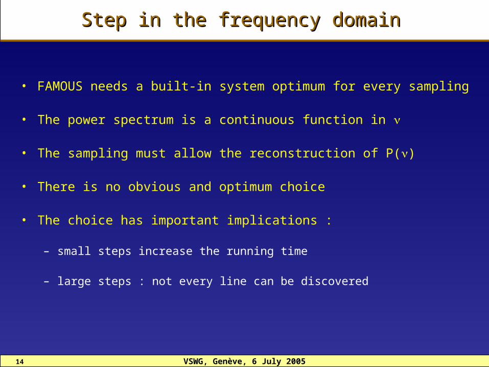
Step in the frequency domainStep in the frequency domain

• FAMOUS needs a built-in system optimum for every sampling

• The power spectrum is a continuous function in

• The sampling must allow the reconstruction of P()

• There is no obvious and optimum choice

• The choice has important implications :

– small steps increase the running time

– large steps : not every line can be discovered


Step in the frequency domainStep in the frequency domain

• In FFT with regular sampling : N+1 data points over T s = 1/T

T

N+1 samples

= T/N

Time domain

=1/2

N/2 frequencies

s = 1/ T

Frequency domain

• In DFT with regular sampling : more freedom on s , but less efficiency


Sampling in frequenciesSampling in frequencies

• High resolution of well chosen spectral lines

– s(t) = cos(2 t), v = 1, 2, …, k in min .. max

• Statistics of the k widths at half-maximum

– k = 1 for uniform time sampling

– k ~ 15 for irregular sampling

• Several protections against peculiar line shapes

• Then s ~ <w>/6

• Resolution good enough to go through all the lines

w1 w2 w3 w4 wk

1.0

0.5

1 2 3 4 k


Largest solvable frequencyLargest solvable frequency

• The trickiest problem met during development

• Related to the generalisation of the Nyquist frequency

• Relatively well founded solution for uniform sampling

– max = Nyquist frequency or multiple

• No natural maximum for irregular sampling

– inverse of the smallest, average, median … interval ?

• Practical solution adopted for FAMOUS :

– Either :

• max user provided recommended solution

– Otherwise : search of a representative timestep

• statistics of the 2-point intervals in the time domain

• then ~ 2nd decile and max = 1/2


PerformancesPerformances


SimulationSimulation

• The simulation generates a periodic or multi-periodic signal

• Sampling can be regular or with some randomness

• s(tk) = 2cos(2/p1* tk) + cos(2/p2* tk)

• Gaussian random noise with = 0.1

– n = 1000 samples

– P = 3, 5, …. days

– T = 500 days

– = 0.5 day (for regular sampling)

– 1/ = 2 cy/day

– Ny. = 1/2 = 1 cy/day


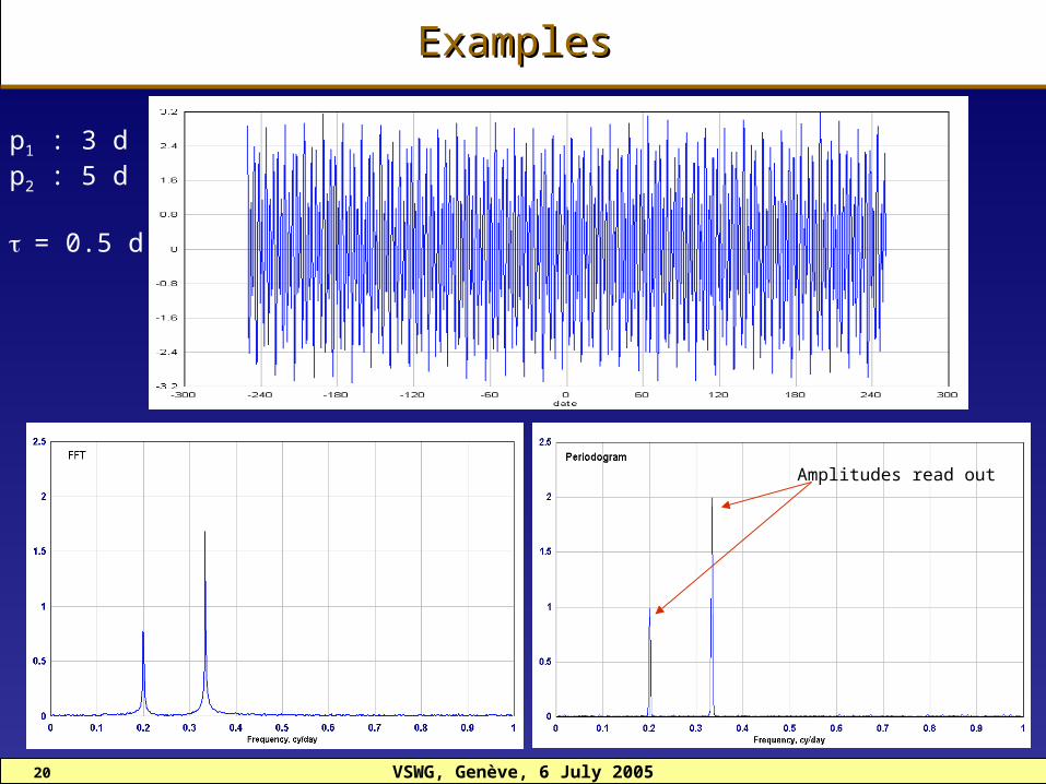
ExamplesExamples

p1 : 3 dp2 : 5 d

= 0.5 d

Amplitudes read out


ExamplesExamples

p1 : 3 dp2 : 5 d

= 0.5 d


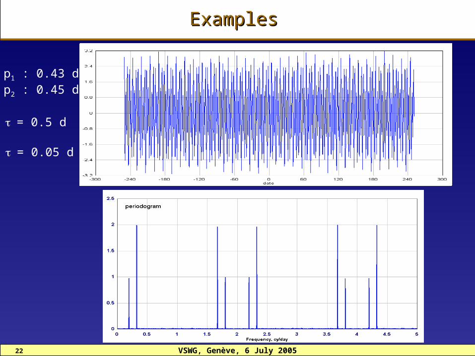
ExamplesExamples

p1 : 0.43 dp2 : 0.45 d

= 0.05 d

= 0.5 d


Examples : random samplingExamples : random sampling

p1 : 3 dp2 : 5 d

= 0.5 d = 0.1Uniform random sampling of 1000 data points over 500 days.

Periods and amplitudes found

2.99998 +/- 0.00002 1.995 +/- 0.005

4.99998 +/- 0.0001 1.005 +/- 0.005

)/2cos()/2cos(2)( 21 PtPttS kkk


Examples : Gaia-like samplingExamples : Gaia-like sampling

= 0.1220 samples over 1600 days.

ii P

tatS 2cos)(

i P a

1 3 22 5 1.53 1 14 7 0.55 20 0.2


Start-P1-P2-P3

- P4-P5

i P a

1 3 22 5 1.53 1 14 7 0.55 20 0.2



Periods amplitudes

3 2.99998 +/- 0.00002 2 1.993 +/- 0.02

5 4.99995 +/- 0.00006 1.5 1.523 +/- 0.02

1 0.99999 +/- 0.00002 1.0 0.990 +/- 0.02

7 7.00008 +/- 0.0003 0.5 0.483 +/- 0.02

20 20.0083 +/- 0.008 0.2 0.187 +/- 0.02

• Results from FAMOUS

i P a

1 3 22 5 1.53 1 14 7 0.55 20 0.2


2-mode Cepheids2-mode Cepheids

• Hip 2085 = TU Cas

– problem known for many years

– large residuals in Hipparcos data with a single period

– well visible in the folded light-curve

date (days)0 150 300 450 600 750 900 1050 1200 1350

8.4

8.2

8

7.8

7.6

7.4

7.2

7

0 0.1 0.2 0.3 0.4 0.5 0.6 0.7 0.8 0.9 18.4

8.2

8

7.8

7.6

7.4

7.2

7

P = 2. 13949 d

• FAMOUS can solve for several unrelated periods

– p1 = 2.1395, p2 = 1.5186 , p3 = 1.1753 days

– a1 = 0.316, a2 = 0.086 , a3 = 0.074 mag


Famous for periodic signalsFamous for periodic signals

• FAMOUS is not specifically designed for periodic signal

• However one can search only one frequency

– in most cases of interest this gives the period

– but : the largest amplitude of a periodic signal can be an harmonic

• therefore a submutiple of the period is found

• With two frequencies : = 2 or 0. 5 tests

• This approach is generalised to locate the fundamental

– search the first frequency (largest amplitude in the 1st

periodogram)

– search over a narrow bandwidth around

– tests to select the fundamental


Eclipsing Binaries I.Eclipsing Binaries I.

Fourier coefficients

EA star with b/a = 0.1

0.1


b/a = 0.0 to 1.0

Eclipsing Binaries II.Eclipsing Binaries II.

-The first harmonics gets larger from Ea to Ec

- the period found may be half the true period


P = 0.594839 dHipparcos P = 0.297187 dFAMOUS

Eclipsing binary : period ?Eclipsing binary : period ?

• Hip 1387 = AQ Tuc


Global exploitation on Hipparcos dataGlobal exploitation on Hipparcos data

• Run over the photometric data of the ~ 2500 periodic variables– periods larger than 2h searched ( 0 to 12 cy/day) key parameter– totally blind search– production of folded light-curves– running time on laptop : 450 s ~ 0.18 s/star

150

80

250

5001500

Stars

20% 80%


Wrong solutions Wrong solutions

HIP 1559 HIP 1805

HIP 3277

HIP 3572HIP 5955

HIP 6350

Factor 2Very different


Wrong solutions ?Wrong solutions ?

HIP 7145

HIP 7417

Factor 2

not foundor

factor 2


Conclusions and Further developmentsConclusions and Further developments

• FAMOUS performs very well to analyse periodic time series

• It is not optimum for pulse-like signals with numerous harmonics

• But it is very efficient as starting method

• More effort on the theory is needed :

– significance and error analysis not complete

– window function for irregular sampling

– better theoretically validated maximum frequency

– relation with sufficient statistics not established

• FAMOUS is freely available on line, with Fortran source, test

files, and the built-in simulator : website of the VSWG or on

ftp.obs-nice.fr/pub/mignard/Famous


Nyquist frequency on irregular samplings

---

F. Mignard

OCA/ Cassiopée


Statement of the problemStatement of the problem

• Aliasing is a well known effect in frequency analysis

– it is conspicuous in regular sampling

– its evidence is less obvious with semi-regular sampling

• depends on underlying quasi-regularity of gaps or observation clustering

– there is no aliasing at all with random sampling

• Aliasing restricts the frequency range in harmonic analysis

– with regular sampling : max = 1/2Nyquist frequency

• From experience : with irregular samplings much higher

frequencies recoverable

– empirical rules applied :

• inverse of min interval

• inverse of mean interval

• no bound

– key parameter for both the science return and runtime efficiency


Aliasing with regular samplingAliasing with regular sampling

2/1)()( andoperator linear with ])2exp[,()( SSPtiTS

Zmkikikmikmi

kitititt kk

)2exp()2exp().2exp())(2exp(

)2exp().2exp()2exp( if 01

)()(;)()(

: has one /1with

PPSS

Signal: X(t) defined in the time domain

sampling : X(tk), t1, t2, … , tn

Spectrum : S() defined in the frequency domain

Power: P() " " "

)()( :but PP )()( PP : symmetry wrt /2


Alias patternAlias pattern

• Any line in 0 < </2 is mirrored infinitely many times at :

,2,1,1,2,,

,2,1,1,2,,

mm

kk

1 2 3 4 5 6

k= 1 k= 2 k= 3m= 1 m= 2 m= 3

21

0


Example with regular samplingExample with regular sampling

cy/d

d5.0,3

2cos2)(

ttT

)(P

N

k=1 k=2m=1 m=2 k=3m=3


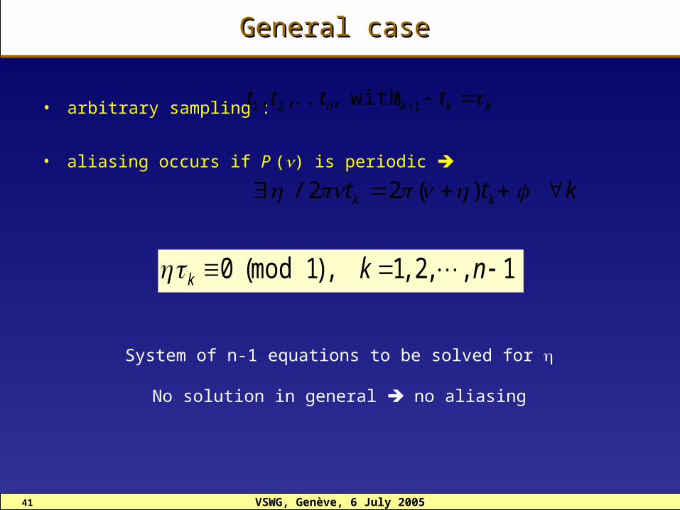
General caseGeneral case

• arbitrary sampling : kkkn ttttt 121 with ...,,,

ktt kk )(22/

1,,2,1,)1mod(0 nkk

System of n-1 equations to be solved for

No solution in general no aliasing

• aliasing occurs if P () is periodic


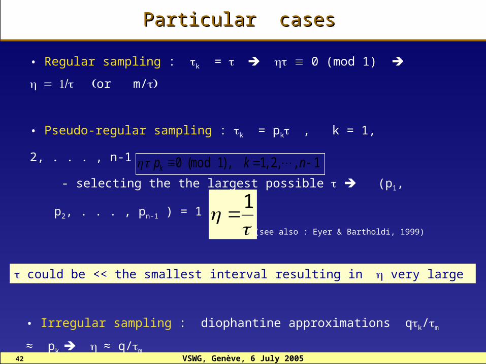
Particular casesParticular cases

• Regular sampling : k = 0 (mod 1) or

m/

• Pseudo-regular sampling : k = pk , k = 1, 2, . . . , n-1

- selecting the the largest possible (p1, p2, . . . , pn-1 ) = 11,,2,1,)1mod(0 nkpk

1

could be << the smallest interval resulting in very large

• Irregular sampling : diophantine approximations qk/m ≈ pk

≈ q/m

(see also : Eyer & Bartholdi, 1999)


Gaia astro samplingGaia astro sampling

• Smallest interval t = 100 mn N~ 7.2 cy/d

– but no aliasing visible

– very small periods can be recovered

cy/d

mn 52,2cos2)(

P

P

ttT )(P

N 52 mn


ConclusionsConclusions

• Better understanding of the aliasing

• Further developments involve higher arithmetics

• Gaia period search puts on safer grounds

Details and proofs in :

F. Mignard, 2005, About the Nyquist Frequency, Gaia_FM_022


Examples : random samplingExamples : random sampling

p1 : 3 dp2 : 5 d

= 0.5 d = 0.1Exponential waiting time sampling of 1000 data points over 500 days.


2.99999 +/- 0.00002 2.017 +/- 0.005

4.99994 +/- 0.0001 0.988 +/- 0.005




p1 : 3 dp2 : 5 d

= 0.1220 samples over 1600 days.





3.000023 +/- 0.000015 2.006 +/- 0.015

5.000036 +/- 0.00008 0.998 +/- 0.015

vswg, genève, 6 july 2005 1 frequency analysis mapping on unusual samplings --- f. mignard oca/...

Documents