volume iii: fate and transport of mercury … · volume iii: fate and transport of mercury in the...

EXCERPT FROM MERCURY STUDY REPORT TO CONGRESS

VOLUME III:

FATE AND TRANSPORT OF MERCURY IN THE ENVIRONMENT

December 1997

Office of Air Quality Planning and Standardsand

Office of Research and Development

U.S. Environmental Protection Agency

http://www.epa.gov/ttn/oarpg/t3/reports/volume3.pdf#page=91

4-1

4. MODEL FRAMEWORK

This section describes the models and modeling scenarios used to predict the environmental fateof mercury. Measured mercury concentrations in environmental media were used when available toparameterize these models. Human and wildlife exposures to mercury were predicted based on modelingresults.

4.1 Models Used

The extant measured mercury data alone were judged insufficient for a national assessment of mercury exposure for humans and wildlife. Thus, the decision was made to model the mercury emissionsdata from the stacks of combustion sources. In this study, there were three major types of modelingefforts: (1) modeling of mercury atmospheric transport on a regional basis; (2) modeling of mercuryatmospheric transport on a local scale (within 50 km of source); and (3) modeling of mercury fate insoils and water bodies into biota, as well as the resulting exposures to human and selected wildlifespecies. The models used for these aspects of this study are described in Table 4-1.

Table 4-1Models Used to Predict Mercury Air Concentrations, Deposition Fluxes,

and Environmental Concentrations

Model Description

RELMAP Predicts average annual atmospheric mercury concentration and wetand dry deposition flux for each 40 km grid in the U.S. due to all2

anthropocentric sources of mercury in the U.S.

ISC3 Predicts annual average atmospheric concentrations and depositionfluxes within 50 km of mercury emission source

IEM-2M Predicts environmental mercury concentrations based on airconcentrations and deposition rates to watershed and water body.

4.2 Modeling of Long-Range Fate and Transport of Mercury

4.2.1 Objectives

The goal of this analysis was to model the emission, transport, and fate of airborne mercury overthe continental U.S. using the meteorologic data for the year of 1989 and the most current emissionsdata. The results of the simulation were intended to be used to answer a number of fundamentalquestions. Probably the most general question was "How much mercury is emitted to the air annuallyover the United States, and how much of that is then deposited back to U.S. soils and water bodies over atypical year?" It is known that year-to-year variations in accumulated precipitation and wind flowpatterns affect the observed quantity of mercury deposited to the surface at any given location. Meteorological data for the year of 1989 was used since most of the continental U.S. experienced near

4-2

normal average weather conditions during that year. A secondary question was that of the contributionby source category to the total amount of mercury emitted and the amount deposited within the U.S. Inorder to answer the questions about the source relative depositions, information on chemical and physicalforms of the mercury emissions from the various source categories was needed since these characteristicsdetermine the rate and location of the wet and dry deposition processes for mercury.

The intent of the analysis was to determine which geographical areas of the United States havethe highest and lowest amounts of deposition from sources using the overall results of the long-rangetransport modeling effort nation-wide. This analysis was expected to contribute understanding of the keyvariables, such as source location, chemical/physical form of emission, or meteorology, that mightcontribute to the outcomes. These long-range modeling efforts were also intended to be used forcomparison with local impact modeling results, essentially to estimate the effects of hypothetical newlocal sources in relation to the estimated effects from long-range transport.

4.2.2 Estimating Impacts from Regional Anthropogenic Sources of Mercury

The impact of mercury emissions from stationary, anthropogenic U.S. sources is not entirelylimited to the local area around the facility. To account for impacts of mercury emitted from many ofthese other non-local sources on the area around a specific source, the long-range transport of mercuryfrom all selected sources has been modeled using the RELMAP (Regional Lagrangian Model of AirPollution) model. The RELMAP model was used to predict the average annual atmospheric mercuryconcentration and the wet and dry deposition flux for each ½ degree longitude by � degree latitude gridcell (approximately 40 km square) in the continental U.S. The emission, transport, and fate of airbornemercury over the continental U.S. was modeled using meteorological data for the year of 1989. Over10,000 mercury emitting cells within the U.S. were addressed; the emission data used were thosepresented in Volume II, Inventory of Anthropogenic Mercury Emissions.

The RELMAP model was originally developed to estimate concentrations of sulfur and sulfurcompounds in the atmosphere and rainwater in the eastern U.S. The primary modification of RELMAPfor this study was the handling of three species of mercury (elemental, divalent, and particulate) andcarbon soot (or total carbon aerosol). Carbon soot was included as a modeled pollutant because carbonsoot concentrations are important in the modeling estimates of the wet deposition of elemental mercury(Iverfeldt, 1991; Brosset and Lord, 1991; Lindqvist et al., 1991).

4.2.3 Description of the RELMAP Mercury Model

Previous versions of the RELMAP are described and evaluated in Eder et al. (1986) and Clark etal. (1992) and a separate description of the initial development of the RELMAP mercury modeling isprovided in Bullock et al. (1997a). Modifications to the RELMAP for atmospheric mercury simulationwere heavily based on recent Lagrangian model developments in Europe (Petersen et al., 1995). Themercury version of the RELMAP was developed to handle three species of mercury: elemental vapor(Hg ), divalent vapor (the mercuric ion, Hg ) and particulate Hg (Hg ), and also aerosol carbon soot. 0 2+

P

Recent experimental work indicates that ozone (Munthe, 1992) and carbon soot (Iverfeldt, 1991; Brossetand Lord, 1991; Linqvist et al., 1991) are both important in determining the wet deposition of Hg . 0

Carbon soot, or total carbon aerosol, was included as a modeled pollutant in the mercury version ofRELMAP to provide necessary information for the Hg wet deposition parameterization. Observed0

ozone (O ) air concentration data for the simulation period were obtained from EPA's Aerometric3

Information Retrieval System (AIRS) data base. Thus, it was not necessary to include O as an explicitly3

modeled pollutant. Methyl mercury was not included in the mercury version of RELMAP because it is

4-3

not yet known if it has a primary natural or anthropogenic source, or if it is produced in the atmosphere. Unless specified otherwise in the following sections, the modeling concepts and parameterizationsdescribed in the EPA users' guide (Eder et al., 1986) were preserved for the RELMAP mercury modelingstudy.

4.2.3.1 Physical Model Structure

RELMAP simulations were originally limited to the area bounded by 25 and 55 degrees northlatitude and 60 and 105 degrees west longitude, and had a minimum spatial resolution of 1 degree in bothlatitude and longitude. For this study, the western limit of the RELMAP modeling domain was movedout to 130 degrees west longitude, and the modeling grid resolution was reduced to ½ degree longitudeby � degree latitude (approximately 40 km square) to provide high-resolution coverage over the entirecontinental U.S.

The original 3-layer puff structure of the RELMAP has been replaced by a 4-layer structure. Thefollowing model layer definitions were used for the RELMAP mercury simulations to account for thedevelopment of deeper nocturnal inversion layers during autumn and winter and higher convectivemixing heights in the spring and summer:

Layer 1 top - 30 to 50 meters above the surface (season-dependent)Layer 2 top - 200 meters above the surfaceLayer 3 top - 700 meters above the surfaceLayer 4 top - 700 to 1500 meters above the surface (month-dependent)

4.2.3.2 Mercury Emissions

Area source emissions were introduced into the model in the lowest layer. Point sourceemissions were introduced into model layer 2 to account for the effective stack height of the point sourcetype in question. Effective stack height is the actual stack height plus the estimated plume rise. Thelayer of emission is inconsequential during the daytime when complete vertical mixing is imposedthroughout the 4 layers. At night, since there is no vertical mixing, area source emissions to layer 1 aresubject to dry deposition while point source emissions to layer 2 are not. Large industrial emissionsources and sources with very hot stack emissions tend to have a larger plume rise, and their effectivestack heights might actually be larger than the top of layer 2. Since, however the layers of the pollutantpuffs remain vertically aligned during advection, the only significant process effected by the layer ofemission is nighttime dry deposition.

Mercury emissions data were grouped into eleven different point-source types and a generalarea-source type. The area source emissions data describe those sources that are too small to beaccounted for individually in pollutant emission surveys. For the RELMAP mercury modeling study,area sources were assumed to emit mercury entirely in the form of Hg gas, while ten of the point source0

types were each assigned mercury speciation profiles based on previous European research (Petersen etal., 1995) and the results of stack testing at a medical waste incinerator in Dade County, Florida (Stevenset al., 1996). These speciation profiles defined the estimated fraction of mercury emitted as Hg , Hg ,0 2+

and Hg . For medical waste incinerator speciation estimates, it was assumed that one-quarter of the HgP2+

emissions measured in the hot stack exhaust would quickly convert to Hg form upon cooling andP

dilution in ambient air. Municipal waste combustors and medical waste incinerators were furthergrouped by the types of air pollution control devices (APCDs) indicated for each plant in the inventoryand separate speciation profiles were assumed for each group based on the assumption that Hg and Hg2+

P

4-4

are preferentially extracted from the waste stream and that Hg is extracted only after all Hg and Hg is0 2+P

removed. The total mercury extraction efficiency for each APCD configuration was based oninformation presented in Volume II, Inventory of Anthropogenic Mercury Emissions. The mercuryemissions inventory for hazardous waste combustors included estimates of the emission speciation foreach plant and no general assumption of speciation profile was required.

There remains considerable uncertainty as to the actual speciation factors for each point sourcetype. A wide variety of alternate emission speciations have been simulated for important groups ofatmospheric mercury sources in order to test the sensitivity of the RELMAP results to the speciationprofiles used (Bullock et al., 1997b). This work showed that the RELMAP modeling results are verystrongly dependent on the assumed emission speciations. The emission speciation profiles used for thisstudy are shown in Table 4-2. The total (non-speciated) mercury emissions inventory used is thatdescribed in Volume II of this Report. Figures 4-1, 4-2 and 4-3 show the total mercury emissions fromall anthropogenic sources in the form of Hg , Hg and Hg , respectively. Speciated data derived from0 2+

P

actual monitoring of sources are a critical research need. These data are needed to establish a clearcausal link between mercury originating from anthropogenic sources and mercury concentrations(projected or actual) in environmental media and/or biota.

Global-scale natural emissions, recycled anthropogenic emissions and current emissions fromanthropogenic sources outside the RELMAP model domain were accounted for by superimposing anambient atmospheric concentration of Hg gas of 1.6 ng/m . This use of a constant background0 3

concentration to account for global-scale and external anthropogenic emissions is the same techniqueused by Petersen et al. (1995). Functional limitations of Lagrangian pollutant parcel modeling preventany explicit treatment of emission sources located outside the spatial domain of the RELMAP as noexternal starting point for parcel trajectories can be defined. Natural and recycled emissions from soilsand water bodies within the model domain cannot be treated explicitly due to the number of simulatedpollutant parcels that would originate from all locations. Even if these natural and recycled parcels wereexplicitly modeled, the prevailing west-to-east atmospheric flow of the mid-latitude northern hemispherewould produce an artificial west-to-east gradient in the simulated effects from these pollutant parcels. The deposition parameterizations described in section 4.2.4.1 were used to simulate the scavenging ofHg from the constant background concentration throughout the entire RELMAP model domain. The0

result was used as an estimate of the deposition of mercury from all natural sources and anthropogenicsources outside the model domain.

4-5

Table 4-2Mercury Emissions Inventory Used in the RELMAP Modeling

Mercury Emission Source Type Emissions(kg/yr)

Speciation Percentages

Hg Hg Hg 0 a 2+ bP

c

Electric Utility Boilers (coal, oil and gas) 46,183 50 30 20

Municipal Waste 50% Control 9,099 40 45 15Combustors 85% Control 219 100 0 0

Standard 17,393 20 60 20

Total 26,711

Commercial and Industrial Boilers 25,650 50 30 20

Medical Waste Incinerators 94% Control 1,365 33 50 17Standard 13,177 2 73 25

Total 14,542

Chlor-Alkali Factories 6,482 70 30 0

Hazardous Waste Incinerators 6,435 58 20 22� � �

Portland Cement Manufacturing 4,355 80 10 10

Residential Boilers 3,244 50 30 20

Pulp and Paper Plants 1,651 50 30 20

Sewage Sludge Incinerators 799 20 60 20

Other Point Sources 3,072 80 10 10

Area Sources 2,721 100 0 0

Hg represents elemental mercury gasa 0

Hg represents divalent mercury gasb 2+

Hg represents particulate mercurycP

The inventory included emissions speciation for each plant. Speciation percentages shown are cumulative for all�

hazardous waste incinerators in the inventory.

4-8

Figure 4-3Hg(p) Emissions from All Anthropogenic Sources (Base)

4-9

4.2.3.3 Carbon Aerosol Emissions

Penner et al. (1993) concluded that total carbon air concentrations are highly correlated withsulfur dioxide (SO ) air concentrations from minor sources. They concluded that the emissions of total2

carbon and SO from minor point sources are correlated as well, since both pollutants result from the2

combustion of fossil fuel. Their data indicate a 35% proportionality constant for total carbon airconcentrations versus SO air concentrations. The RELMAP mercury model estimated total carbon2

aerosol emissions using this 35% proportionality constant and SO emissions data for minor sources2

obtained by the National Acidic Precipitation Assessment Program (NAPAP) for the year 1988. Much ofthese SO emissions data had been previously analyzed for use by the Regional Acid Deposition Model2

(RADM). For the portion of the RELMAP mercury model domain not covered by the RADM domain,state by state totals of SO emissions were apportioned to the county level on the basis of weekday2

vehicle-miles-traveled data since recent air measurement studies have indicated that aerosol elementalcarbon can be attributed mainly to transportation source types (Keeler et al., 1990). The county leveldata were then apportioned by area to the individual RELMAP grid cells. Total carbon soot wasassumed to be emitted into the lowest layer of the model.

4.2.3.4 Ozone Concentration

Ozone concentration data were obtained from U.S. EPA's Aerometric Information RetrievalSystem (AIRS) and the Acidmodes experimental air sampling network. AIRS and Acidmodes data wereavailable hourly. For each observation site in the AIRS database, the ozone concentrations werecomputed for the two mid-day RELMAP time steps by using the mean concentration value during thetwo corresponding time periods (1000-1300 and 1400-1600 local time). The mean of these two mid-dayvalues was used to estimate the ozone concentration for the time steps after 1600 local time and before1000 local time the next morning. This previous-day average was used at night since ground-level ozonedata are not valid for the levels aloft where the wet removal of elemental mercury was assumed to beoccurring. Finally, an objective interpolation scheme using 1/r weighted averaging was used to produce2

complete ozone concentration grids from observational data for each time step, with a minimum value of20 ppb imposed.

It is recognized that, by estimating nighttime elevated ozone concentrations from observedground-level ozone concentrations of the previous day, we do not resolve any possible advection ofozone concentration gradients during the nighttime hours. Since it is well documented that ground levelobservations of ozone concentration do not correlate well with actual elevated concentrations at night,we opted not to use nighttime surface-level data. Since observations of elevated ozone concentrationwere not available except in rare instances, we believe that estimation based on previous-dayobservations were our only recourse short of explicit modeling of ozone advection and chemistry withinthe RELMAP which is not currently possible. By not resolving the advection of ozone gradients, it ispossible that nighttime precipitation could co-locate with erroneous estimates of ozone concentration. Given that high ozone concentrations do not normally occur with precipitation, these erroneous estimatesof ozone concentration would most likely be too high, leading to an artificial bias toward high simulatedHg oxidation and subsequent wet deposition. Since there remains considerable uncertainty about the0

true nature of Hg oxidation in cloud water and its controlling effect on wet deposition, the risk of0

modeling errors related to nighttime ozone concentration estimates from previous-day observations wasdeemed acceptable.

4-10

4.2.3.5 Lagrangian Transport and Deposition

In the model, each pollutant puff begins with an initial mass equal to the total emission rate of allsources in the source cell multiplied by the model time-step length. For mercury, as for most otherpollutants previously modeling using RELMAP, emission rates for each source cell were defined fromemission inventory data, and a time step of three hours was used. The initial horizontal area of each puffwas set to 1200 km , instead of the standard initial size of 2500 km , in order to accommodate the finer2 2

grid resolution used for the mercury modeling study; however, the standard horizontal expansion rate of339 km per hour was not changed. Although each puff was defined with four separate vertical layers,2

each layer of an individual puff was advected through the model cell array by the same wind velocityfield. Thus, the layers of each puff always remained vertically stacked. Wind field initialization data fora National Weather Service prognostic model, the Nested Grid Model (NGM), were obtained for each0000 and 1200 GMT initialization time during the year of 1989. Wind analyses for the � =0.897 verticalp

level of the NGM were used to define the translation of the puffs across the model grid, except during themonths of January, February, and December, when the � =0.943 vertical level was used to reflect a morep

shallow mixed layer. � is a pressure-based vertical coordinate equal to (p-p )/(p -p ). Thep top surface top

� =0.897 and � =0.943 levels approximate elevations above ground level of 1000 m and 500 m,p p

respectively. These wind fields at 12-h intervals were linearly interpolated in time to produce the windfields used to define puff motion for each 3-h RELMAP time step.

Pollutant mass was removed from each puff by the processes of wet deposition, dry deposition,diffusive air exchange between the surface-based mixed layer and the free atmosphere, and, in the caseof reactive species, chemical transformation. The model parameterizations for these processes arediscussed in Section 4.2.4. Hourly precipitation data for the entire year of 1989 from the TD-3240 dataset of the U.S. National Climatic Data Center were used to estimate the wet removal of all pollutantspecies modeled. A spatial and temporal sub-grid-scale analysis of these hourly observations wasperformed using a process previously developed for sulfur wet deposition modeling (Bullock, 1994). This process provides resolution of precipitation variability not obtainable by simple numericalaveraging of all observations within each grid cell and time step. Wet and dry deposition mass totalswere accumulated and average surface-level concentrations were calculated on a monthly basis for eachmodel cell designated as a receptor. Except for cells in the far southwest and eastern corners of themodel domain where there were no wind data, all cells were designated as receptors for the mercurysimulation. When the mass of pollutant in a puff declines through deposition, vertical diffusion ortransformation to a user-defined minimum value, or when a puff moves out of the model grid, the puffand its pollutant load is no longer tracked. The amount of pollutant in the terminated puff is taken intoaccount in monthly mass balance calculations so that the integrity of the model simulation is assured. Output data from the model includes monthly wet and dry deposition totals and monthly average airconcentration for each modeled pollutant, in every receptor cell.

4.2.4 Model Parameterizations

4.2.4.1 Chemical Transformation and Wet Deposition

The simplest type of pollutant to model with RELMAP is the inert type. To model inertpollutants, one can simply omit chemical transformation calculations for them, and not be concernedwith chemical interactions with the other chemical species in the model. In the mercury version ofRELMAP, particulate mercury and total carbon were each modeled explicitly as inert pollutant species. Reactive pollutants are normally handled by a chemical transformation algorithm. RELMAP wasoriginally developed to simulate sulfur deposition, and the algorithm for transformation of sulfur dioxide

W(Hg0) �

k1

k2

�1

HHg

� [O3]aq � (1 � K3 �csoot

r)

4-11

to sulfate was independent of wet deposition. For gaseous mercury, however, the situation is morecomplex. Since there are no gaseous chemical reactions of mercury in the atmosphere which appear tobe significant (Petersen et al., 1995), for this modeling study mercury was assumed to be reactive only inthe aqueous medium. Elemental mercury has a very low solubility in water, while oxidized forms ofmercury and particle bound mercury readily find their way into the aqueous medium through dissolutionand particle scavenging, respectively. Worldwide observations of atmospheric mercury, however,indicate that particulate mercury is generally a minor constituent of the total mercury loading (Iverfeldt,1991) and that gaseous elemental mercury (Hg ) is, by far, the major component. Swedish measurements0

of large north-to-south gradients of mercury concentration in rainwater without corresponding gradientsof atmospheric mercury concentration suggest the presence of physical and chemical interactions withother pollutants in the precipitation scavenging process (Iverfeldt, 1991). Aqueous chemical reactionsincorporated into the mercury version of RELMAP were based on research efforts in Sweden (Iverfeldtand Lindqvist, 1986; Lindqvist et al., 1991; Munthe et al., 1991; Munthe and McElroy, 1992; Munthe,1992) and Canada (Schroeder and Jackson, 1987; Schroeder et al., 1991).

Unlike other pollutants that have been modeled with RELMAP, mercury has wet deposition andchemical transformation processes that are interdependent. A combined transformation/wet-removalscheme proposed by Petersen et al. (1995) was used. In this scheme, the following aqueous chemicalprocesses were modeled when and where precipitation is present:

1) oxidation of dissolved Hg by ozone yielding Hg0 2+

2) catalytic reduction of this Hg by sulfite ions2+

3) adsorption of Hg onto carbon soot particles suspended in the aqueous medium2+

Petersen et al. (1995) shows that these three simultaneous reactions can be considered in the formulationof a scavenging ratio for elemental mercury gas as follows:

where, k is the second order rate constant for the aqueous oxidation of Hg by O equal to 1 3

0

4.7 x 10 M s ,7 -1 -1

k is the first order rate constant for the aqueous reduction of Hg by sulfite ions equal 22+

to 4.0 x 10 s ,-4 -1

H is the dimensionless Henry's Law coefficient for Hg (0.18 in winter, 0.22 in spring and Hg0

autumn, and 0.25 in summer as calculated from Sanemasa (1975)),[O ] is the aqueous concentration of ozone,3 aq

K is a model specific adsorption equilibrium constant (5.0 x 10 m g ),3-6 4 -1

c is the total carbon soot aqueous concentration, andsoot

r is the assumed mean radius of soot particles (5.0 x 10 m).-7

[O3]aq �

[O3]gas

HO3

4-12

[O ] is obtained from this equation:3 aq

where H is the dimensionless Henry's Law coefficient for ozone (0.448 in winter, 0.382 in spring andO3

autumn, and 0.317 in summer as calculated from Seinfeld (1986)). c is obtained from the simulatedsoot

atmospheric concentration of total carbon aerosol using a scavenging ratio of 5.0 x 10 .5

The model used by Petersen et al. (1995) defined one-layer cylindrical puffs, and the Hg0

scavenging layer was defined as the entire vertical extent of the model. The RELMAP defines 4-layerpuffs to allow special treatment of surface-layer and nocturnal inversion-layer processes. It was believedthat, due to the low solubility of Hg in water, the scavenging process outlined above would only take0

place effectively in the cloud regime, where the water droplet surface-area to volume ratio is high, andnot in falling raindrops. Thus the Hg wet scavenging process was applied only in the top two layers on0

RELMAP, which extends from 200 meters above the surface to the model top.

For the modeling study described in Petersen et al. (1995), the wet deposition of Hg was treated2+

separately from that of Hg . Obviously, any Hg dissolved into the water droplet directly from the air0 2+

could affect the reduction-oxidation balance between the total concentration of Hg and Hg in the0 2+

droplet. Since the solubility and scavenging ratio for Hg is much larger than that for Hg , and since air2+ 0

concentrations of Hg are typically larger than those of Hg , separate treatment of Hg wet deposition0 2+ 2+

was deemed acceptable for this modeling study also. Thus, process 2 above was only considered as amoderating factor for the oxidation of dissolved Hg .0

In the exposure analysis in Volume III, there was no attempt to develop a new interactingchemical mechanism for simultaneous Hg and Hg wet deposition. Although Hg was recognized as a0 2+ 2+

reactive species in aqueous phase redox reactions, it was, in essence, modeled as an inert species just likeparticulate mercury and total carbon soot. With the rapid rate at which the aqueous Hg reduction2+

reaction is believed to occur in the presence of sulfite, it is possible that an interactive cloud-waterchemical mechanism might produce significant conversion of scavenged Hg to Hg , with possible2+ 0

release of that Hg into the gaseous medium.0

Wet deposition of Hg , particulate mercury, and total carbon soot in the mercury version of2+

RELMAP were modeled with the same scavenging ratios used by Petersen et al. (1995). The gaseousnitric acid scavenging ratio of 1.6 x 10 has been applied for Hg since the water solubilities of these-6 2+

two pollutant species are similar. For particulate mercury, a scavenging ratio of 5.0 x 10 was used,-5

based on experiences in long-range modeling of lead in northern Europe. As previously mentioned, ascavenging ratio of 5.0 x 10 was also used for total carbon soot. These scavenging ratios for Hg ,-5 2+

particulate mercury, and total carbon soot were applied to all four layers of the RELMAP in thecalculation of pollutant mass scavenging by precipitation.

4.2.4.2 Dry Deposition

Recent experimental data indicate that elemental mercury vapor does not exhibit a net drydepositional flux to vegetation until the atmospheric concentration exceeds a rather high compensationpoint well above the global background concentration of 1.6 ng m (Hanson et al., 1994). This-3

4-13

compensation point is apparently dependent on the surface or vegetation type and represents a balancebetween emission from humic soils and dry deposition to leaf surfaces (Lindberg et al., 1992). Since theemission of mercury from soils was accounted for with a global-scale ambient concentration and not anactual emission of Hg , for consistency, there was no explicit simulation of the dry deposition of Hg .0 0

For Hg during daylight hours, a dry deposition velocity table previously developed based on2+

HNO data (Walcek et al., 1985; Wesely, 1986) was used. The dry deposition characteristics of HNO3 3

and Hg should be similar since their water solubilities are similar and gaseous dry deposition to2+

vegetation involves solution into moist plant tissue. This dry deposition velocity data, shown in Table 4-3, provided season-dependent values for 11 land-use types under six different Pasquill stabilitycategories. Based on the predominant land-use type and climatological Pasquill stability estimate ofeach RELMAP grid cell, and the season for the month being modeled, the dry deposition velocity valuesshown in Table 4-3 were used for the daytime only. For nighttime, a value of 0.3 cm/s was used for allgrid cells since the RELMAP does not have the capability of applying land-use dependent dry depositionat night. Since the nighttime dry deposition was applied only to the lowest layer of the model and novertical mixing is assumed for nighttime hours, all Hg modeled would be quickly depleted from the2+

lowest model layer by larger dry deposition velocities.

For Hg , Petersen et al. (1995) used a dry deposition velocity of 0.2 cm/s at all times andP

locations. Lindberg et al. (1991) suggests that the dry deposition of Hg seems to be dependent on foliarP

activity. In the RELMAP mercury model, daytime dry deposition velocities for Hg were calculatedP

using a FORTRAN subroutine developed by the California Air Resources Board (CARB, 1987). Aparticle density of 2.0 g cm and diameter of 0.3 µm was assumed. Table 4-4 shows the wind speed (u)-3

used for each Pasquill stability category in the calculation of deposition velocity from the CARBsubroutine, while Table 4-5 shows the roughness length (z ) used for each land-use category. During0

simulated night, all cells used 0.02 cm/s as the dry deposition velocity for Hg . Lindberg et al. (1991)P

suggested a value of 0.003 cm/s for non-vegetated land, but since the RELMAP can not model land-usedependent dry deposition at night, the value of 0.02 cm/s was used for these cells by necessity.

For total carbon soot, daytime dry deposition velocities were also calculated using the CARBsubroutine. A particle density of 1.0 g/cm and radius of 0.5 µm was assumed. For nighttime, a dry3

deposition velocity of 0.07 cm/s was used for all seasons and land-use types.

Petersen et al. (1995) used local dry deposition factors for Hg and Hg in addition to the normal2+P

model treatments to remedy an assumed underestimation of the dry deposition rate for mercury speciesemitted near the ground due to an underestimation of the ground-level concentration from instantaneouscomplete vertical mixing in their model. This local deposition factor was the fraction of the emissionsfrom a grid cell that were assumed to dry deposit within that grid cell by processes not otherwisesimulated by the dry deposition parameterization. In the RELMAP mercury model, we compensated forthis underestimation of local deposition by simulating all depositions before pollutant parcel transport ineach model timestep. In essence, the parcel was held over its location of origin for 3 h before beingtransported away by the horizontal wind. Thus, no use of a local deposition factor in the RELMAPmodeling was deemed necessary.

4-14

Table 4-3Dry Deposition Velocity (cm/s) for Divalent Mercury (Hg )2+

Season Land-Use CategoryPasquill Stability Category

A B C D E F

Winter

Urban 4.83 4.80 4.61 4.30 2.79 0.36Agricultural 1.32 1.30 1.20 1.05 0.46 0.15Range 1.89 1.86 1.73 1.52 0.73 0.19Deciduous Forest 3.61 3.57 3.34 3.02 1.68 0.29Coniferous Forest 3.61 3.57 3.34 3.02 1.68 0.29Mixed Forest/Wetland 3.49 3.46 3.27 2.99 1.77 0.29Water 1.09 1.07 0.98 0.85 0.38 0.13Barren Land 1.16 1.14 1.06 0.92 0.39 0.31Non-forested Wetland 2.02 2.00 1.89 1.70 0.96 0.21Mixed Agricultural/Range 1.62 1.60 1.48 1.30 0.60 0.17Rocky Open Areas 1.98 1.95 1.81 1.58 0.73 0.20

Spring


Summer


Autumn


4-15

Table 4-4Wind Speeds Used for Each Pasquill Stability Category

in the CARB Subroutine Calculations

Stability Category Wind Speed (m/s)

A 2.0B 3.0C 4.0D 5.0E 3.0F 2.0

Table 4-5Roughness Length Used for Each Land-Use Category

in the CARB Subroutine Calculations

Land-Use CategoryRoughness Length (meters)

spring-summer autumn-winter

Urban 0.5 0.5Agricultural 0.15 0.05Range 0.12 0.1Deciduous Forest 0.5 0.5Coniferous Forest 0.5 0.5Mixed Forest/Wetland 0.4 0.4Water 10 10Barren Land 0.1 0.1Non-forested Wetland 0.2 0.2Mixed Agricultural/Range 0.135 0.075Rocky Open Areas 0.1 0.1

-6 -6

4.2.4.3 Vertical Exchange of Mass with the Free Atmosphere

Due to the long atmospheric lifetime of mercury, the RELMAP was adapted to simulate acontinuous exchange of mass between the surface-based mixed layer and the free atmosphere above. Inthe modeling of Petersen et al. (1995), a depletion of pollutant from the mixed layer was simulated at theend of the day based on estimates of the subsidence of the mixed-layer top due to the horizontaldivergence of the wind field. For the RELMAP modeling, a pollutant depletion rate of 5 percent per 3-hour timestep was chosen to represent this diffusive mass exchange. When compounded over a 24-hourperiod, this depletion rate removes 33.6% of an inert, non-depositing pollutant. This compares to anaverage diffusive mass loss of 30-40% per day in the European modeling study (Petersen, personalcommunication). Since a portion of all modeled species of mercury can deposit to the surface before this

4-16

diffusive mass loss is calculated in the RELMAP, the effective mass loss is somewhat less than 33.6%per day from this process.

4.3 Modeling the Local Atmospheric Transport of Mercur y in Source Emissions

The program used to model the transport of the anthropogenic mercury within 50 km of anemissions source was the ISC3 gas deposition model, obtained from USEPA’s Support Center forRegulatory Air Models (SCRAM) website (the program is called GDISCDFT). This model has a gas drydeposition model that was applied in this study.

4.3.1 Phase and Oxidation State of Emitted Mercury

Reports describe several forms of mercury detected in the emissions from the selected sources. Primarily, these include elemental mercury (Hg ) and inorganic mercuric (Hg ). Generally, only total0 2+

mercury has been measured in emission analyses. The reports of MHg in emissions are imprecise. It isbelieved that, if MHg is emitted from industrial processes and combustion sources, the quantities emittedare much smaller than emissions of Hg and Hg . Only Hg and Hg were considered in the air0 +2 0 +2

dispersion modeling.

The two types of mercury species considered in the emissions are expected to behave quitedifferently once emitted from the stack. Hg , due to its high vapor pressure and low water solubility, is0

not expected to deposit close to the facility. In contrast, Hg , because of differences in these properties,2+

is expected to deposit in greater quantities closer to the emission sources.

At the point of stack emission and during atmospheric transport, the contaminant is partitionedbetween two physical phases: vapor and particle-bound. The mechanisms of transport of these twophases are quite different. Particle-bound contaminants can be removed from the atmosphere by bothwet deposition (precipitation scavenging) and dry deposition (gravitational settling, Brownian diffusion). Vapor phase contaminants may also be depleted by these processes, although historically their mainimpacts were considered to be through absorption into plant tissues (air-to-leaf transfer) and humanexposure occurred through inhalation.

For the present analysis, the vapor/particle (V/P) ratio was assumed to be equal to the V/P ratioas it would exist in the emissions plume. It is recognized that this is a simplification of reality, as the ratiowhen emitted from the stack is likely to change as the distance from the stack increases. It was assumedthat 25% of the divalent emissions from an individual source would attach to particles in the plume. Theuncertainty in this estimate is acknowledged. Essentially, particulate mercury is not measured at stack tipbut has been measured in plumes downwind from local sources. It is assumed that the divalent fractionbinds to sulfur particles.

The particle-size distribution may differ from one combustion process to another, depending onthe type of furnace and design of combustion chamber, composition of feed/fuel, particulate matterremoval efficiency and design of air pollution control equipment, and amount of air in excess ofstoichiometric amounts that is used to sustain the temperature of combustion. The particle sizedistribution used is as estimate of the distribution within an ambient air aerosol mass and not at stack tip. Based on this assumption, an aerosol particle distribution based on data collected by Whitby (1978) wasused. This distribution is split between two modes: accumulation and coarse particles. The geometricmean diameter of several hundred measurements indicates that the accumulation mode dominates particlesize, and a representative particle diameter for this mode is 0.3 microns. The coarse particles are formed

4-17

largely from mechanical processes that suspend dust, sea spray and soil particles in the air. Arepresentative diameter for coarse particles is 5.7 microns. The fraction of particle emissions assigned toeach particle class is approximated based on the determination of the density of surface area of eachrepresentative particle size relative to total surface area of the aerosol mass. Using this method,approximately 93% and 7% of the total surface area is estimated to be in the 0.3 and 5.7 micron diameterparticles, respectively.

Table 4-6Representative Particle Sizes and Size Distribution

Assumed for Divalent Mercury Particulate Emissions

Representative Particle Size Assumed Fraction of Particle(microns)* Emissions in Size Category

0.3 0.93

5.7 0.07*These values are based on the geometric means of aerosol particle

distribution measurements as described in Whitby (1978).

The speciation estimates for the model plants were made from thermal-chemical modeling ofmercury compounds in flue gas, from the interpretation of bench and pilot scale combustor experimentsand from interpretation of available field test results. The amount of uncertainty surrounding theemission rates data varies for each source. There is also a great deal of uncertainty with respect to thespecies of mercury emitted.

Although the speciation may change with distance from the local source, for this analysis it wasassumed that there were no plume reactions that significantly modified the speciation at the local source. Because of the differences in deposition characteristics of the two forms of mercury considered, theassumption of no plume chemistry is a particularly important source of uncertainty.

4.3.2 Modeling the Deposition of Mercury

Once emitted from a source, the mercury may be deposited to the ground via two main processes:wet and dry deposition. Wet deposition refers to the mass transfer of dissolved gaseous or suspendedparticulate mercury species from the atmosphere to the earth's surface by precipitation, while drydeposition refers to such mass transfer in the absence of precipitation.

The deposition properties of the two species of mercury addressed in stack emissions, elementaland divalent mercury, are considered to be quite different. Due to its higher solubility, divalent mercuryvapor is thought to deposit much more rapidly than elemental mercury. However, at this time noconclusive data exist to support accurate quantification of the deposition rate of divalent mercury vapor. In this analysis, nitric acid vapor is used as a surrogate for Hg vapor based on their similar solubility in++

water. Whether a pollutant is in the vapor form or particle-bound is also important for estimatingdeposition, and each is treated separately.

Dry deposition is estimated by multiplying the predicted air concentration at ground level by adeposition velocity. For particles, the dry deposition velocity is estimated using the CARB algorithms

4-18

(CARB 1986) that represent empirical relationships for transfer resistances as a function of particle size,density, surface area, and friction velocity. For the vapor phase fraction for elemental mercury, a singledry deposition velocity of 0.06 cm/s is assumed. This is based on the average of the winter and summerdeposition velocities presented in Lindberg et al. (1992) for forests. Although it is generallyacknowledged that elemental mercury dry deposits with a (net) rate much lower than divalent mercuryvapor, the precise value is uncertain, and there can be considerable variability with season and time ofday. Additionally, dry deposition of elemental mercury may not occur at all unless the air concentrationis sufficiently high. Preliminary research (Hanson et al.1995) indicates that under some experimentalconditions no dry deposition occurs unless the air concentration is at least 10 ng/m ; this was termed a3

compensation point (the value at which dry deposition would being to occur is expected to depend onmany factors, including time of year and the type of flora present). These preliminary results were notspecifically addressed in the current study; however, sensitivity analyses were conducted in order todetermine the possible impact that such a compensation point might have on the predicted dry depositionof elemental mercury (see Section 5.3.4.1 below).

In ISC-GAS, the dry deposition of divalent mercury vapor was modeled by calculating a drydeposition velocity for each hour using the assumptions usually made for nitric acid for the inputparameters (see EPA 1996; User’s Guide for the Gas Dry Deposition Model, page inserts to the User’sGuide for the Industrial Source Complex (ISC3) Dispersion Models). Ultimately, using the assumptionshere, the average predicted dry deposition velocity was about 2.9 cm/s for divalent mercury vapor, whichis essentially the average of the values used in the RELMAP modeling for coniferous forests.

Table 4-7Parameter Values Assumed for Calculation of Dry Deposition Velocities for

Divalent Mercury Vapor

Parameter Value

Molecular diffusivity (cm2/sec) 0.1628

Solubility enhancement factor 109

Pollutant reactivity 800

Mesophyll resistance 0

Henry’s law coefficient 2.7e-7

Wet deposition is estimated by assuming that the wet deposition rate is characterized by ascavenging coefficient which depends on precipitation intensity and particle size. For particles, thescavenging ratios used are from Jindal and Heinold (1991) (see Figure 4-4). For the vapor phasefraction, a scavenging coefficient is also used, but it is calculated using estimates for the washout ratio,which is the ratio of the concentration of the chemical in surface-level precipitation to the concentrationin surface-level air. Because of its higher solubility, divalent mercury vapor is assumed to be washed outat significantly higher rates than elemental mercury vapor. The washout ratio for divalent mercury vaporwas selected based on an assumed similarity between scavenging for divalent mercury and gaseous nitricacid. This is based on Peterssen (1995), and the value used for the washout ratio for divalent vapor was

4-19

1.6x10 . The washout ratio for elemental mercury vapor was assumed to be 1200. This is a calculated6

value based on the model of Peterssen et al. (1995), with a soot concentration 0.

Figure 4-4 Wet Deposition Scavenging Ratios Used in Local Scale Air Modeling for Particulate-Bound

Mercur y (Jindal and Heinold 1991)

4-20

Table 4-8Air Modelin g Parameter Values Used in the Exposure Assessment: Generic Parameters

Parameter Value Used in Study

Particle Density (g/cm ) 1.83

Surface Roughness Length (m)* 0.30

Anemometer Height (m) 10

Wind Speed Profile Exponents

Stability Class A 0.07

Stability Class B 0.07

Stability Class C 0.10

Stability Class D 0.15

Stability Class E 0.35

Stability Class F 0.55

Terrain Adjustment Factors

Stability Class A 0.5

Stability Class B 0.5

Stability Class C 0.5

Stability Class D 0.5

Stability Class E 0

Stability Class F 0

Distance Limit for Plume Centerline (m) 10

Model Run Options

Terrain Adjustment Yes

Stack-tip Downwash No

Building Wake Effects No

Transitional Plume Rise Yes

Buoyancy-induced dispersion Yes

Calms Processing Option No

This is used to estimate deposition velocities for particles.a

4-21

4.3.3 Rationale and Utility of Model Plant Approach

Mercury is generally present as a low-level contaminant in combustion materials (e.g., coal ormunicipal solid waste) and industrial material (for more information on mercury in emissions refer toVolume II of this Report). During combustion and high-temperature industrial processes, mercury isvolatilized from these materials. Because of its high volatility, it is difficult to remove mercury from thepost-combustion air stream. As a consequence, mercury is released to the atmosphere. As notedpreviously, anthropogenic mercury emissions are not the only source of mercury to the atmosphere. Mercury may be introduced into the atmosphere through volatilization from natural sources such as lakesand soils. Consequently, it is difficult to trace the source(s) of mercury concentrations in environmentalmedia and biota. For this reason it is also difficult to gain an understanding of contribution to thoseconcentrations.

For this assessment it was not possible to model the emission impact of every mercury emissionsource in each selected industrial and combustion class. Consequently, the actual mercury emission dataand facility characteristics for any specific source were not modeled. Instead, a model plant approach, asdescribed in Appendix C, was utilized to develop facilities which represent actual sources. Model plantswere developed to represent four source categories; namely municipal waste combustors, coal and oil-fired boilers, medical waste incinerators, and chlor-alkali plants. The model plants were designed tocharacterize the mercury emission rates as well as the atmospheric release processes exhibited by actualfacilities in the source class. The modeled facilities were not designed to exhibit extreme sources (e.g.,the facility with the highest mercury emission rate) but rather to serve as a representative of theindustrial/combustion source class.

This assessment took as its starting point the results of measured mercury emissions fromselected anthropogenic sources. Using a series of fate models and hypothetical constructs, mercuryconcentrations in environmental media, pertinent biota and ultimately mercury contact with human andwildlife receptors were predicted. An effort was made to estimate the amount of receptor contact withmercury as well as the oxidative state and form of mercury contacted.

In taking the model plant approach, it was realized that there would be a great deal of uncertaintysurrounding the predicted fate and transport of mercury as well as the ultimate estimates of exposure. The uncertainty can be divided into modeling uncertainty and parameter uncertainty. Parameteruncertainty can be further subdivided into uncertainty and variability depending on the level to which aparticular model parameter is understood. A limited quantitative analysis of uncertainty is presented. Itis also hoped that the direction of future research can be influenced toward reducing the identifieduncertainties which significantly impact key results.

4.3.4 Development and Description of Model Plants

Model plants representing four source classes were developed to represent a range of mercuryemissions sources. The source categories were selected for the exposure assessment based on theirestimated annual mercury emissions as a class or their potential to be localized point sources of concern. The categories selected were these:

4-22

� municipal waste combustors (MWCs),� medical waste incinerators (MWIs),� utility boilers, and � chlor-alkali plants (CAP).

Parameters for each model plant were selected after evaluation of the characteristics of a givensource category and current knowledge of mercury emissions from that source category. Importantvariables for the mercury risk assessment included mercury emission rates, mercury speciation andmercury transport/deposition rates. Important model plant parameters included stack height, stackdiameter, stack volumetric flow rate, stack gas temperature, plant capacity factor (relative averageoperating hours per year), stack mercury concentration, and mercury speciation. Emission estimateswere assumed to represent typical emission levels emitted from existing sources. Table 4-9 shows theprocess parameters assumed for each model plant considered in this analysis (for details regarding thesevalues, see Appendix C).

4.3.5 Hypothetical Locations of Model Plants

There are a variety of geographic aspects that can influence the impacts of mercury emissionsfrom an anthropogenic source. These aspects include factors that affect the environmental chemistry of apollutant and the physics of plume dispersion. Environmental chemistry can include factors such as theamount of wet deposition in a given area. Factors affecting plume dispersion include terrain, winddirection and average wind speed.

Because wet deposition may be an important factor leading to mercury exposures, especially forthe more soluble species emitted, the meteorology of a location was used as a selection criterion. Twodifferent types of meteorology were deemed necessary to characterize the environmental fate andtransport of mercury: an arid/semi-arid site and a humid site. The humidity of an area was based on totalyearly rainfall. (See Appendix B).

Terrain features refer to the variability of the receptor height with respect to a local source. Broadly speaking, there were two main types of terrain used in the modeling: simple, and complex. Simple terrain is defined as a study area that is relatively level and well below stack top (rather, theeffective stack height). Complex terrain referred to terrain that is not simple, such as source located in avalley or a source located near a hill. This included receptors that are above or below the top of the stackof the source. Complex terrain can effect concentrations, plume trajectory, and deposition. Due to thecomplicated nature of plume flow in complex terrain, it is probably not possible to predict impacts incomplex terrain as accurately as for simple terrain. In view of the wide range of uncertainty inherent inaccurately modeling the deposition of the mercury species considered, the impacts posed by complexterrain were not incorporated in the local scale analysis.

Two generic sites are considered: a humid site east of 90 degrees west longitude, and a morearid site west of 90 degrees west longitude (these are described in Appendix B). The primary differencesbetween the two sites as parameterized were the assumed erosion characteristics for the watershed andthe amount of dilution flow from the water body. The eastern site had generally steeper terrain in thewatershed than for the other site. A circular drainage lake with a diameter of 1.78 km and average depthof 5 m, with a 2 cm benthic sediment depth was modeled at both sites. The watershed area was 37.3 km . 2

4-23

Table 4-9Process Parameters for Model Plants

Model Plant Plant Size (% of (ft) Diameter Rate Percent Velocity (°F)Capacity Stack Height Stack Hg Emission Speciation Exit Exit Temp.

year) (ft) (kg/yr) (Hg /Hg /Hg ) (m/sec)0 2+ P

Large Municipal 2,250 90% 230 9.5 220 60/30/10 21.9 285Waste tons/dayCombustors

Small Municipal 200 tons/day 90% 140 5 20 60/30/10 21.9 375WasteCombustors

Large 1500 lb/hr 88% 40 2.7 4.58 33/50/17 9.4 175CommercialHMI capacityWaste Incinerator (1000 lb/hr(Wetscrubber) actual)

Large Hospital 1000 lb/hr 39% 40 2.3 23.9 2/73/25 16 1500HMI Waste capacityIncinerators (667 lb/hr(Good actual)Combustion)

Small Hospital 100 lb/hr 27% 40 0.9 1.34 2/73/27 10.4 1500HMI Waste capacityIncinerators (67 lb/hr(1/4 actual)sec.Combustion)

Large Hospital 1000 lb/hr 39% 40 2.3 0.84 33/50/17 9.0 175HMI Waste capacityIncinerators (667 lb/hr(Wet Scrubber) actual)

Small Hospital 100 lb/hr 27% 40 0.9 0.05 33/50/17 5.6 175HMI Waste capacityIncinerators (Wet (67 lb/hrScrubber) actual)

Large Coal-fired 975 65% 732 27 230 50/30/20 31.1 273Utilit y Boiler Megawatts

Medium 375 65% 465 18 90 50/30/20 26.7 275Coal-fired Utility MegawattsBoiler

Small Coal-fired 100 65% 266 12 10 50/30/20 6.6 295Utilit y Boiler Megawatts

Medium Oil-fired 285 65% 290 14 2 50/30/20 20.7 322Utilit y Boiler Megawatts

Chlor-alkali plant 300 tons 90% 10 0.5 380 70/30/0 0.1 Ambientchlorine/day

Hg = Elemental Mercurya 0

Hg = Divalent Vapor Phase Mercuryb 2+

Hg = Particle-Bound MercurycP

4-24

4.4 Modeling Mercury in a Watershed

Atmospheric mercury concentrations and deposition rates estimated from RELMAP and ISC3drive the calculations of mercury in watershed soils and surface waters. The soil and waterconcentrations, in turn, drive calculations of concentrations in the associated biota and fish, whichhumans and other animals are assumed to consume. The watershed model used for this report, IEM-2M,was adapted from the more general IEM-2 methodology (U.S. EPA, 1990; U.S. EPA, 1994, externalreview draft) to handle mercury fate in soils and water bodies.

4.4.1 Overview of the Watershed Model

IEM-2M simulates three chemical components -- elemental mercury, Hg (C ), divalent mercury,01

HgII (C ), and methyl mercury, MHg (C ). In the previous version of IEM-2, these components were2 3

assumed to be in a fixed ratio with each other as specified by the fraction elemental (f ) and fraction1

methyl (f ). This updated version calculates the fractions in each component based on specified or3

calculated rate constants. The equations and parameters are described below, and implemented in anExcel spreadsheet. The model is parameterized for several hypothetical scenarios as described inChapter 5.

IEM-2M is composed of two integrated modules that simulate mercury fate using mass balanceequations describing watershed soils and a shallow lake, as illustrated in Figures 4-5 and 4-6. The massbalances are performed for each mercury component, with internal transformation rates linking Hg ,0

HgII, and MHg. Sources include wetfall and dryfall loadings of each component to watershed soils andto the water body. An additional source is diffusion of atmospheric Hg vapor to watershed soils and the0

water

Figure 4-5Configuration of Hypothetical Water Body and Watershed Relative to Local Source

4-25

Definitions for Figure 4-6

C total mercury concentration in upper soil ng/gsoil

C total mercury concentration in water body ng/Lw

C vapor phase mercury concentration in air ng/matm3

D average dry deposition to watershed �g/m -yryds2

D average wet deposition to watershed �g/m -yryws2

Figure 4-6Overview of the IEM-2M Watershed Modules

4-26

body. Sinks include leaching of each component from watershed soils, burial of each component fromlake sediments, volatilization of Hg and MHg from the soil and water column, and advection of each0

component out of the lake.

At the core of IEM-2M are 9 differential equations describing the mass balance of each mercurycomponent in the surficial soil layer, in the water column, and in the surficial benthic sediments. Theequations are solved for a specified interval of time, and predicted concentrations are output at fixedintervals. For each calculational time step, IEM-2M first performs a terrestrial mass balance to obtainmercury concentrations in watershed soils. Soil concentrations are used along with vapor concentrationsand deposition rates to calculate concentrations in various food plants. These are used, in turn, tocalculate concentrations in animals. IEM-2M next performs an aquatic mass balance driven by directatmospheric deposition along with runoff and erosion loads from watershed soils. MHg concentrationsin fish are derived from dissolved MHg water concentrations using bioaccumulation factors (BAF).

IEM-2 was developed to handle individual chemicals, or chemicals linked by kinetictransformation reactions. IEM-2M is expanded to include specific kinetic transformation rates affectingmercury components in soil, water, and sediments -- oxidation, reduction, methylation, anddemethylation. These transformation rates are driven by specified rate constants. Volatilization kineticsare included as a transfer reaction driven by specified chemical properties and environmental conditions.

The nature of this methodology is quasi-steady with respect to time and homogeneous withrespect to space. While it tracks the buildup of soil and water concentrations over the years given asteady depositional load and long-term average hydrological behavior, it does not respond to unsteadyloading or meteorological events. There are, thus, limitations on the analysis and interpretations imposedby these simplifications. The model's calculations of average water body concentrations are less reliablefor unsteady environments, such as streams, than for more steady environments, such as lakes.

4.4.2 Description of the Watershed Soil Module

The IEM-2M watershed soil module calculates surface soil concentrations, including dissolved,sorbed, and gas phases, as illustrated in Figure 4-7. The model accounts for three routes of contaminantentry into the soil: deposition of particle-bound contaminant through dryfall; deposition through wetfall;and diffusion of vapor phase contaminant into the soil surface. The model also accounts for fourdissipation processes that remove mercury from the surface soils: volatilization (diffusion of gas phaseout of the soil surface); runoff of dissolved phase from the soil surface; leaching of the dissolved phasethrough the soil horizon; and erosion of particulate phase from the soil surface. Key assumptions in thewatershed soil module were these:

� Soil concentrations within a depositional area are assumed to be uniform within the area,and can be estimated by the following key parameters: dry and wet contaminantdeposition rates, a diffusion-driven gaseous exchange rate with the atmosphere, a set ofsoil transformation rates, a soil bulk density, and a soil mixing depth.

� The partitioning of mercury components among soil water, soil particle, and soil gasphases can be described by partition coefficients and Henry’s Law constants.

4-27

Definitions for Figure 4-7

C vapor phase chemical concentration in air µg/matm3

D average dry deposition to watershed mg/yryds

D average wet deposition to watershed mg/yryws

C total chemical concentration in soil mg/Lst

C reaction product concentration in soil mg/Lst'

C background chemical concentration in soil mg/Lb

C chemical concentration in soil gas µg/mgs3

chemical concentration in soil water mg/LCDs

C chemical concentration on soil particles µg/gps

H Henry's Law constant atm-m /mole3

R universal gas constant atm-m /mole-�K3

T temperature �KK soil/water partition coefficient L/kgds

Figure 4-7Overview of the IEM2 Soils Processes

Csi � Sci � BD

Vs dCsi

d t� LSD,i � STs,i � SLs,i

STs,i � �ksT � Vs � Csj

SLs,i � ksx � Vs � Csi

Cig � Ciw � Cis

4-28

4.4.2.1 Development of Soil Mass Balance Equations

The concentration of constituent �i� in watershed soils can be expressed per unit volume (C , insi

mg/L) or per unit mass (Sc , in mg/kg), where BD is soil bulk density (dry weight basis), in kg/L:i

Given constant steady depositional loading L (g/yr) onto a surficial soil layer, the following massSD,i

balance equation governs the mass response:

where:V = watershed soil volume (m )s

3

S = total transformation source in the soil layer (g/yr) Ts,i

S = total transport and transformation loss in the soil layer (g/yr). Ls,i

A simple first-order transformation source from constituent C would be given by:sj

where: ks = first-order transformation rate constant (yr ) T

-1

Similarly, a simple first-order loss process would be given by:

where: ks = total first-order loss rate constant (yr )x

-1

The basic mass balance equation is applied to three interacting mercury components. For eachcomponent �i,� three phases in local equilibrium are calculated -- gas phase (C , �g/m ), aqueous phaseig

3

(C , mg/L), and solid phase (C , �g/g):iw is

The fraction of each component �i� in each phase -- f , f , and f -- is calculated using partitionig iw is

coefficients and properties of the soil, as described in a section below.

ksr

C1T � C2T

kso

ksdm

C2T � C3T

ksm

C3T � C1T

ksmd

Cig � Cia

ksdiff

4-29

The three mercury components are linked by a set of transformation reactions, includingoxidation of total elemental mercury, reduction and methylation of total divalent mercury, anddemethylation of total methyl mercury by two pathways:

These are modeled as first-order processes, each a function of environmental conditions, where:

ks = oxidation rate constant (yr ) o-1

ks = reduction rate constant (yr ) r-1

ks = methylation rate constant (yr ) m-1

ks = demethylation rate constant (yr )dm-1

ks = mer cleavage demethylation rate constant (yr ) md-1

Each mercury component is also subject to a set of transport processes, including leaching andrunoff of dissolved phase, erosion of particulate phase, and volatilization of gas phase. These aremodeled as first-order processes, where ks is the leaching rate constant (yr ), ks is the runoff rateL R

-1

constant (yr ), and ks is the erosion rate constant (yr ). Each of these rate constants is a function of-1 -1e

environmental conditions. While leaching, runoff, and erosion are strictly loss processes from the soil,volatilization is a diffusive exchange process between soil and atmosphere:

where: ks = diffusive exchange volume (m /yr) diff

3

This diffusive exchange leads to an atmospheric loading that partially balances the volatile loss from thesoil. The net loss rate is the product of ks and the concentration gradient (C -C ). For modelingdiff ig ia

purposes, it is convenient to divide this process into a diffusive loading term and a first-order loss term,where ks is the volatilization loss rate constant (yr ). These are developed in the sections below.v

-1

Using the calculated phase fractions, three differential equations can be written to describe themercury mass balance in soil:

Vs � dCs1

dt� LSD,1 � ksr �Vs � Cs2 � ksmd�Vs � Cs3

� ( ksv,1�kso�ksRO�ksL�kse) � Vs � Cs1

Vs � dCs2

dt� LSD,2 � kso �Vs � Cs1 � ksdm�Vs � Cs3

� (ksr�ksm�ksRO�ksL�kse) � Vs � Cs2

Vs � dCs3

dt� LSD,3 � ksm�Vs � Cs2

� (ksv,3�ksdm�ksmd�ksRO�ksL�kse) � Vs � Cs3

LSD,i � (Dydwi � Dywwi � LDIF,i) � As

LDIF,i �

ksdiff,i

As

� Ca,i � 10�6

4-30

The major model coefficients are described in more detail in the sections below.

4.4.2.2 Loads to Watershed Soils

The total atmospheric loading term for component �i� -- L in the mass balance equations -- isSD,i

the sum of the wetfall, dryfall, and vapor diffusion fluxes:

where: Dydw = yearly-average dry depositional flux of component �i� (g/m -yr) i

2

Dyww = yearly-average wet depositional flux of component �i� (g/m -yr) i2

L = yearly-average vapor diffusion flux of component �i� (g/m -yr) DIF,i2

The vapor diffusion flux is calculated from the diffusion volume and the atmospheric concentration,normalized to the surface area:

where: ks = diffusive exchange volume (m /yr)diff,i

3

A = surface area of the watershed soil element (m ) s2

C = vapor phase atmospheric concentration for component �i� (µg/m ) a,i3

ksdiff �Di � As � �v

zr

� 3.15×107 � 10�4

Cig � (Hi/RTK) � Ciw

Cis � Kdi � Ciw

CiT � Cig ��v � Ciw ��w � Cis�BD

4-31

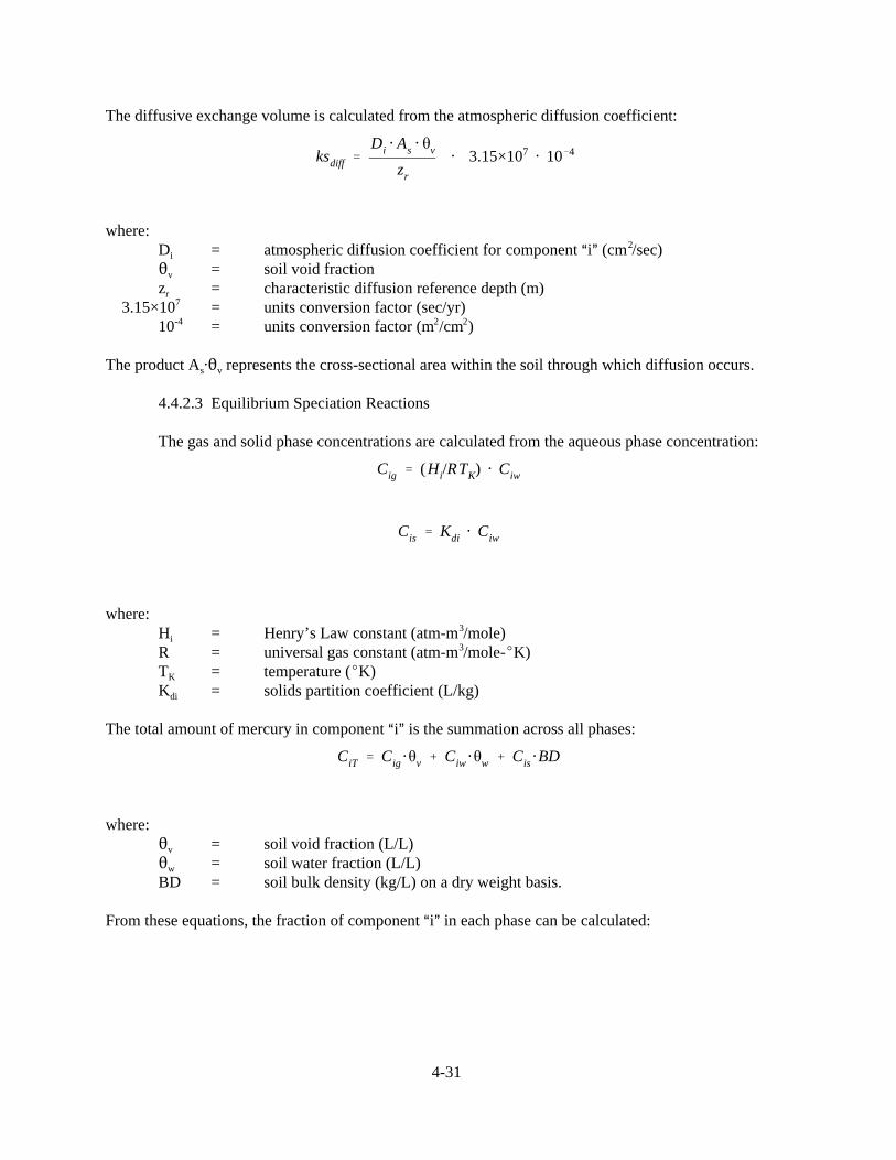
The diffusive exchange volume is calculated from the atmospheric diffusion coefficient:

where: D = atmospheric diffusion coefficient for component �i� (cm /sec) i

2

� = soil void fractionv

z = characteristic diffusion reference depth (m) r

3.15×10 = units conversion factor (sec/yr) 7

10 = units conversion factor (m /cm ) -4 2 2

The product A�� represents the cross-sectional area within the soil through which diffusion occurs.s v

4.4.2.3 Equilibrium Speciation Reactions

The gas and solid phase concentrations are calculated from the aqueous phase concentration:

where: H = Henry’s Law constant (atm-m /mole) i

3

R = universal gas constant (atm-m /mole-�K) 3

T = temperature (�K) K

K = solids partition coefficient (L/kg) di

The total amount of mercury in component �i� is the summation across all phases:

where: � = soil void fraction (L/L)v

� = soil water fraction (L/L) w

BD = soil bulk density (kg/L) on a dry weight basis.

From these equations, the fraction of component �i� in each phase can be calculated:

fig �

(Hi/RTK) ��v

(Hi/RTK) ��v � �w � Kdi �BD

fiw �

�w


fis �

Kdi �BD


ksRO,i �Ro

zs

�fiw

�w

4-32

4.4.2.4 Transformation Processes in Watershed Soils

As described above, five transformation reactions are modeled as first-order rates. Rateconstants are directly specified and applied to the bulk concentration (all phases) to give internal masstransformation loadings. The oxidation loading ks�V �C is subtracted from the Hg mass balanceo s s1

0

equation and added to the HgII equation. The reduction loading ks�V �C is subtracted from the HgIIr s s2

equation and added to the Hg equation. The methylation loading ks�V �C is subtracted from the HgII0m s s2

equation and added to the MHg equation. The demethylation loading ks�V �C is subtracted from thedm s s3

MHg equation and added to the HgII equation. Finally, the mer demethylation loading ks�V �C ismd s s3

subtracted from the MHg equation and added to the Hg equation.0

There is evidence that reduction in soil is mediated by sunlight, is proportional to soil watercontent, and occurs most rapidly within the upper 5 mm of the soil surface (Carpi and Lindberg, 1997). As a result, the input reduction rate constant k is normalized to a reference depth z of 5 mm and tors r

100% water content. The actual reduction rate constant ks used in the model is the product of k , ther rs

soil water content � and the ratio of the reference depth to the depth of the soil layer z /z .w r s

4.4.2.5 Transport and Transfer Processes in Watershed Soils

The total transport loss of component �i� from the soil is the sum of the loss rates due toleaching, runoff, erosion, and volatilization. In the governing mass balance equations, these loss ratesare expressed as the product of a loss rate constant, the total component concentration, and the soilvolume. The runoff loss constant is a function of the runoff volume and the dissolved fraction ofcomponent �i�:

where: Ro = average annual runoff (m/yr) z = upper soil layer depth (m) s

� = volumetric water content (dimensionless; cm /cm )w3 3

ksL,i �P � I � Ro � EV

zs

�fiw

�s

kse,i �Xe � SD� ER

zs

�fis

1000� BD

ksv � Vs � Csi � ksdiff,i � Cig

ksv �

ksdiff,i

Vs

�fig�v

4-33

f = aqueous fraction of component �i� concentration. iw

The first term times the soil volume is the annual runoff volume in m /yr, while the second term times3

the total concentration is the aqueous concentration in the runoff in g/m .3

The leaching loss constant is a function of the leaching volume and the dissolved fraction ofcomponent �i�:

where: P = average annual precipitation (m/yr)I = average annual irrigation (m/yr)EV = average annual evapotranspiration (m/yr).

The first term times the soil volume is the annual percolation volume in m /yr , while the second term3

times the total concentration is the aqueous concentration in percolating water, in g/m .3

The erosion loss constant is a function of the erosion mass and the particulate fraction ofcomponent �i�:

where: X = unit soil loss (kg/m -yr; see Eq [9-3], IED; Wischmeier and Smith, 1978)e

2

SD = sediment delivery ratio ER = particle enrichment ratio BD = soil dry density (g/cm ) 3

f = sorbed fraction of the total component �i� concentration . is

The first term times the soil volume is the annual erosion mass in kg/yr, while the second term times thetotal concentration is the sorbed concentration on the eroding particles in g/kg.

The volatilization rate constant ks can be derived from the diffusive exchange volume and gasv

phase concentration:

where: ks = diffusive exchange volume (m /yr)diff,i

3

V = soil layer volume (m )s3

ksv � 3.15×103Di � �v

zs � zr

�fig

�v

4-34

� = void fraction. v

Substituting in the expression for ks gives the volatilization rate constant in terms of the atmosphericdiff,i

diffusivity and the gaseous fraction of component �i� in the soil:

where: D = atmospheric diffusivity (cm /sec) i

2

z = soil thickness (m) s

z = characteristic diffusive mixing depth (m) r

3.15×10 = units conversion factor (sec/yr � m /cm ) 3 2 2

� = soil void fractionv

f = gaseous fraction of the total component �i� concentration. ig

The first term times the soil volume is the annual gas diffusion volume in m /yr, while the second term3

times the total concentration is the gas phase concentration in the void space in g/m .3

4.4.3 Description of the Water Body Module

The IEM-2M water body module estimates water column as well as bed sediment concentrationsin a shallow lake. Water column concentrations included dissolved, sorbed to suspended sediments andtotal (sorbed plus dissolved, or total contaminant divided by total water volume). This framework alsoprovides three concentrations for the bed sediments: dissolved in pore water, sorbed to bed sediments,and total. The model accounts for five routes of contaminant entry into the water body: erosion ofmercury sorbed to soil particles; runoff of dissolved mercury in runoff water; deposition of particle-bound mercury through wetfall; deposition of particle-bound mercury through dryfall; and diffusion ofvapor phase Hg into the water body. The model also accounts for three dissipation processes that0

remove mercury from the water body: volatilization of dissolved phase Hg and MHg from the water0

column; removal of total mercury via "burial" from the surficial bed sediment layer; and advection oftotal mercury from the water column via outflow. The burial rate is a function of the deposition of bioticand abiotic solids from the water column to the bed; it accounts for the fact that much of the soil erodinginto a water body annually is incorporated into bottom sediment. The impact to the water body wasassumed to be uniform. This tends to be more realistic for smaller water bodies as compared to largerivers or lakes. Key features and assumptions in the surface water body module include the following.

� The partitioning of mercury components between the water column and suspended biotic andabiotic solids, and between pore water and sediment particles is in local equilibrium as describedby a set of partition coefficients.

� Atmospheric mercury wetfall and dryfall loads are handled as a constant average flux.

� Surface runoff mercury loadings are estimated as a function of the dissolved concentration ofmercury in the surficial soil water (calculated by the soil module as a function of time) and thespecified annual water runoff.

Vw dCwt

d t� LT � Vfx�Cwt � Rsw� (Cdb�Cdw)

� [vs�Csw � vsB�CBw � vrs �Cbt] �Aw

� Swt � kv�Aw �Cdw

Vb dCbt

d t� � Rsw� (Cdb�Cdw) � Sbt

� [vs�Csw� vsB�CBw � (vrs�vb) �Csb] �Aw

4-35

� Soil erosion mercury loadings are calculated as a function of the sorbed concentration ofmercury in the surficial soil layer (calculated by the soil module as a function of time), togetherwith the calculated annual soil erosion, a sediment delivery ratio, and an enrichment ratio. Thesediment delivery ratio serves to reduce the total potential amount of soil erosion (where the totalpotential erosion equals the unit erosion rate in kg/m multiplied by the watershed area, in m )2 2

reaching the water body. This parameter accounts for the observation that most of the erodedparticles mobilized within a watershed during a year deposit prior to reaching the water body. The enrichment ratio accounts for the fact that eroding soils tend to be lighter in texture, moreabundant in surface area, and higher in organic carbon. All these characteristics lead toconcentrations in eroded soils that tend to be higher than those in situ soils.

� Diffusive mercury loadings from the atmosphere are calculated as a function of a specifiedatmospheric vapor concentration, the calculated dissolved water column concentration, and thecalculated transfer velocity. The dissolved concentration in a water body is driven towardequilibrium with the vapor phase concentration above the water body. At equilibrium, gaseousdiffusion into the water body is matched by volatilization out of the water body. This specifiedair concentration is an output of the atmospheric transport model.

� The rate of contaminant burial in bed sediments is estimated as a function of the rate at whichbiotic and abiotic solids deposit from the water column onto the surficial sediment layer minusthe rate at which they resuspend to the water column. Burial represents a permanent sink oferoded soil and mercury concentrations scavenged from the water column.

� Separate transformation rate constants allow for the calculation of mercury component fractionsin the water column and benthic sediments.

In the following sections, the mass balance equations and the equilibrium state equations thatlink the concentrations are developed.

4.4.3.1 The Water Body Equations

Given the loading of mercury from atmospheric deposition and the surrounding watershed, thefollowing mass balance equations govern the concentration response in the water column and surficialbenthic sediment layer of a shallow lake:

where:

Rsw �

Esw � Aw � �bs

zb

Cis � Ciw � CiB

4-36

C = total water column concentration (mg/L)wt

C = total benthic concentration (mg/L)bt

C = dissolved water column concentration (mg/L)dw

C = dissolved benthic concentration (mg/L)db

C = particulate abiotic water column concentration (mg/L)sw

C = particulate biotic water column concentration (mg/L)bw

C = particulate (sorbed) benthic concentration (mg/L) sb

C = atmospheric concentration (�g/m ) a3

V = water column volume (m )w3

V = benthic volume (m )b3

L = total loading (g/year)T

Vf = dilution flow (m /year)x3

R = pore water diffusion volume (m /year)sw3

A = surface area (m )w2

v = settling velocity for abiotic solids (m/year)s

v = settling velocity for biotic solids (m/year)sB

v = resuspension velocity (m/year)rs

v = burial velocity (m/year) b

S = net transformation source in the water column (g/yr)wt

S = net transformation source in the benthic sediment layer (g/yr)bt

The pore water diffusion volume is calculated as:

where:E = pore water diffusion coefficient (m /year)sw

2

� = benthic porosity (L /L)bs w

z = surficial benthic layer depth (m)b

The first term in the water column mass balance equation describes external loading, while thesecond term describes advective export. The third term covers net pore water exchange with the surficialbenthic layer, and is also present in the benthic sediment equation. The fourth term gives net depositionof particulate mercury, including settling of abiotic and biotic solids and resuspension of benthic solids. These processes are also represented in the benthic sediment equation. The fifth term in the watercolumn equation gives the net internal transformation source, while the last term gives the netvolatilization loss.

The benthic sediment mass balance equation contains terms for pore water exchange, internaltransformation source, and net solids transport, which includes deposition, resuspension, and burial.

These basic equations are applied to three interacting mercury components. For each component�i� in the water column, three phases in local equilibrium are calculated -- aqueous phase (C , mg/L),iw

abiotic solid phase (C , �g/g), and biotic solid phase (C , �g/g):is iB

kwr kbr

Cwt,1 � Cwt,2 Cbt,1 � Cbt,2

kwo kbo

kwdm kbdm


kwm kbm


kwmd kbmd

4-37

In the sediments, two phases in local equilibrium are calculated -- aqueous pore water phase (C , mg/L)db

and sediment phase (C , �g/g). The fraction of each component �i� in each phase -- f , f , and f insb dw,i sw,i Bw,i

the water column and f and f in the sediments -- is calculated using partition coefficients anddb,i sb,i

properties of the solids and sediment, as described in a section below.

The three mercury components are linked by a set of first-order transformation reactions,including oxidation of total elemental mercury, reduction and methylation of total divalent mercury, anddemethylation of total methyl mercury by two pathways:

where: kw = water column oxidation rate constant (yr )o

-1

kb = benthic oxidation rate constant (yr )o-1

kw = water column reduction rate constant (yr )r-1

kb = benthic reduction rate constant (yr )r-1

kw = water column methylation rate constant (yr )m-1

kb = benthic methylation rate constant (yr )m-1

kw = water column demethylation rate constant (yr )dm-1

kb = benthic demethylation rate constant (yr )dm-1

kw = water column mer cleavage demethylation rate constant (yr )md-1

kb = benthic mer cleavage demethylation rate constant (yr )md-1

Each of these rate constants is a function of environmental conditions. Their values are specified as inputto the IEM-2M model.

Each mercury component is also subject to a set of transport processes, including advectiveexport of all phases in the water column, volatilization and pore water exchange of dissolved phase, andsettling, resuspension, and burial of particulate phase. These are modeled as first-order processes asdescribed in the general water column and benthic sediment mass balance equations above. Volatilization is modeled as a surficial �thin-film� exchange process in which the dissolved concentrationin the water column is driven toward equilibrium with the atmosphere:

Vw dCw,i

d t�volatilization � Kv,i � Aw � Cdw,i �

Ca,i � 10�6

Hi/RTK

Vw � dCwt,1

dt� LT1 � Vs� (ksRO� kse) �Cs1 � kwr �Vw �Cwt,2 � kwmd�Vw �Cwt,3

� Vfx � Rsw� fdw,1 � (kwv,1� kwo) �Vw � (vs� fsw,1� vsB� fBw,1) �Aw �Cwt,1

� Rsw� (fdb,1/�bs) � vrs � fsb,1�Aw �Cbt,1

Vw � dCwt,2

dt� LT2 � Vs� (ksRO� kse) �Cs2 � kwo �Vw �Cwt,1 � kwdm�Vw �Cwt,3

� Vfx � Rsw� fdw,2 � (kwr � kwm) �Vw � (vs� fsw,2� vsB� fBw,2) �Aw �Cwt,2


Vw � dCwt,3

dt� LT3 � Vs� (ksRO� kse) �Cs3 � kwm �Vw �Cwt,2

� Vfx � Rsw� fdw,3 � (kwv,3� kwmd� kwdm) �Vw � (vs� fsw,3� vsB� fBw,3) �Aw �Cwt,3


4-38

where: K = conductivity of component �i� through the air-water interface (m/yr)v,i

H = Henry’s Law constant for component �i� (m -atm/mole)i3

R = Universal Gas constant (atm-m /mole-�K)3

T = water temperature (�K)K

C = component �i�, vapor phase air concentration (µg/m )a,i3

For modeling purposes, it is convenient to divide this process into a diffusive loading term and a first-order loss term, where kw is the volatilization loss rate constant (yr ). These terms are developed inv,i

-1

the sections below.

Using the calculated phase fractions, six differential equations for the three mercury componentsin water column and sediments can be expressed in their mass balance form, grouping constants andmodel parameters within brackets:

Vb � dCbt,1

dt� Rsw� fdw,1 � (vs� fsw,1� vsB� fBw,1) �Aw �Cwt,1 � kbr �Vb �Cbt,2

� kbmd�Vb �Cbt,3 � Rsw� (fdb,1/�bs) � (vrs � vb) � fsb,1�Aw � (kbo) �Vb �Cbt,1

Vb � dCbt,2

dt� Rsw� fdw,2 � (vs� fsw,2� vsB� fBw,2) �Aw �Cwt,2 � kbo�Vb � Cbt,1

� kbdm�Vb �Cbt,3 � Rsw� (fdb,2/�bs) � (vrs � vb) � fsb,2�Aw � (kbr � kbm) �Vb �Cbt,2

Vb � dCbt,3

dt� Rsw� fdw,3 � (vs� fsw,3� vsB� fBw,3) �Aw �Cwt,3 � kbm�Vb � Cbt,2

� Rsw� (fdb,3/�bs) � (vrs � vb) � fsb,3�Aw � (kbmd� kbdm) �Vb �Cbt,3

Vw � dSw

d t� � LSe�As�103

� Vfx � vs�Aw �Sw � vrs �Aw �SB

Vw � dSBio

d t� � LSB�Aw � Vfx � kmort�Vw � vsB�Aw �SBio

Vb � dSB

d t� � vs�Sw � vsB�SBio �Aw � (vrs � vmin � vb) �Aw �SB

4-39

Combined with the soil mercury equations expressed in the previous section, there are nine massbalance differential equations to solve for nine state variables -- elemental, divalent, and methyl mercuryin the soil, water column, and benthic sediments. These differential equations have constant parametersand can be solved for specified time intervals using a standard ODE solver. The following sectionsdescribe how the model parameters in the water body differential equations are calculated or specified.

4.4.3.2 The Solids Balance Equations

The abiotic and biotic solids must be modeled in order to predict the dissolved and particulatemercury fractions. These determine the amount of mercury lost through deposition and burial, and alsoinfluence the bioavailability of methyl mercury in the water column. The differential equationsdescribing the fate of watershed-derived solids in the water column (S ), internally-generated bioticw

solids in the water column (S ), and total solids in the benthic sediments (S ) are given by:Bio B

Sw �

LSe�As�103� vrs�Aw�SB

Vfx � vs�Aw

SBio �

LSB�Aw

Vfx � kmort�Vw � vsB�Aw

vB �

vs�Sw � vsB�SBio� (vrs � vmin) �SB

SB

LT,i � LDep,i � LRI,i � LR,i � LE,i � LDif,i

4-40

where: L = watershed solids erosion load (kg/m -yr)Se

2

L = net internal production of biotic solids (g/m -year)SB2

k = phytoplankton mortality rate (yr )mort-1

v = mineralization rate for upper benthic solids (m/year)min

For long-term average calculations using average watershed loading and waterbody productivity, S ,w

S , and S can be assumed to be at steady-state. If S , v , v , v , and k are specified, then the waterBio B B s sB rs mort

column solids concentrations and the burial velocity can be calculated from:

4.4.3.3 Loads to the Water Body

The total chemical load term L in the mass balance equation is the sum of the loadings for eachT

component "i." Component loadings included wet and dry deposition, impervious and pervious runoff,erosion, and atmospheric diffusion:

where:L = total component "i" load to the water body (g/yr)T,i

L = deposition of particle bound component "i" (g/yr)Dep,i

L = runoff load from impervious surfaces (g/yr)RI,i

L = runoff load from pervious surfaces (g/yr)R,i

L = soil erosion load (g/yr)E,i

L = diffusion load for vapor phase component "i" (g/yr)Dif,i

The runoff and erosion loads required estimation of average contaminant concentration inwatershed soils that comprise the depositional area. These concentrations were developed in terrestrialsections above.

Load due to direct deposition -- The load to surface waters via direct deposition is solved as follows:

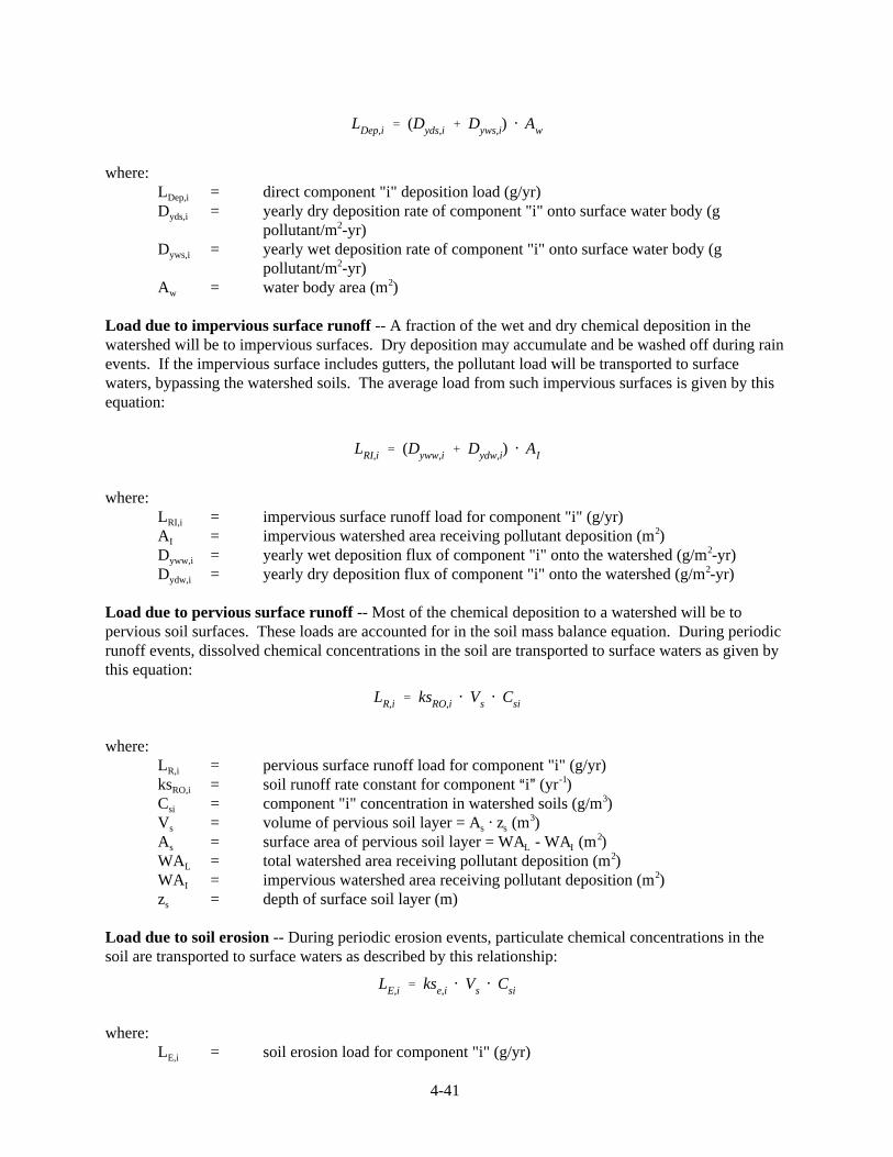
LDep,i � (Dyds,i � Dyws,i) � Aw

LRI,i � (Dyww,i � Dydw,i) � AI

LR,i � ksRO,i � Vs � Csi

LE,i � kse,i � Vs � Csi

4-41

where:L = direct component "i" deposition load (g/yr)Dep,i

D = yearly dry deposition rate of component "i" onto surface water body (gyds,i

pollutant/m -yr)2

D = yearly wet deposition rate of component "i" onto surface water body (gyws,i

pollutant/m -yr)2

A = water body area (m )w2

Load due to impervious surface runoff -- A fraction of the wet and dry chemical deposition in thewatershed will be to impervious surfaces. Dry deposition may accumulate and be washed off during rainevents. If the impervious surface includes gutters, the pollutant load will be transported to surfacewaters, bypassing the watershed soils. The average load from such impervious surfaces is given by thisequation:

where:L = impervious surface runoff load for component "i" (g/yr)RI,i

A = impervious watershed area receiving pollutant deposition (m )I2

D = yearly wet deposition flux of component "i" onto the watershed (g/m -yr)yww,i2

D = yearly dry deposition flux of component "i" onto the watershed (g/m -yr)ydw,i2

Load due to pervious surface runoff -- Most of the chemical deposition to a watershed will be topervious soil surfaces. These loads are accounted for in the soil mass balance equation. During periodicrunoff events, dissolved chemical concentrations in the soil are transported to surface waters as given bythis equation:

where:L = pervious surface runoff load for component "i" (g/yr)R,i

ks = soil runoff rate constant for component �i� (yr )RO,i-1

C = component "i" concentration in watershed soils (g/m )si3

V = volume of pervious soil layer = A � z (m )s s s3

A = surface area of pervious soil layer = WA - WA (m )s L I2

WA = total watershed area receiving pollutant deposition (m )L2

WA = impervious watershed area receiving pollutant deposition (m )I2

z = depth of surface soil layer (m)s

Load due to soil erosion -- During periodic erosion events, particulate chemical concentrations in thesoil are transported to surface waters as described by this relationship:

where:L = soil erosion load for component "i" (g/yr)E,i

LDif,i � Kv,i � Aw �Ca,i � 10�6

Hi/RTK

fdw,i �1

1 � Kdw,i �Sw�10�6� KBio,i �SBio�10�6

fsw,i �Kdw,i �Sw�10�6


fBw,i �KBio,i �SBio�10�6


4-42

ks = soil erosion loss rate constant for component �i� (yr )e,i-1

Load due to gaseous diffusion -- The volatilization equation presented above is divided into a diffusiveloading term and a loss term in IEM-2M. The diffusive loading term is given by:

where:L = diffusive loading rate for component "i" (g/yr)Dif,i

K = overall transfer rate, or conductivity for component "i" (m/yr)v,i

A = surface area of water body (m )w2

C = component "i" vapor phase air concentration over water body (µg/m )a,i3

H = component "i" Henry's Constant (atm-m /mole)i3

R = universal gas constant, 8.206·10 atm-m /mole-�K-5 3

T = water body temperature (�K)K

10 = units conversion factor (g/µg)-6

This treatment of volatilization is based on the well-known two-film theory (Whitman, 1923), asimplemented in standard chemical fate models (Burns, et al., 1982, Ambrose, et al., 1988). Theequations for K are presented in the volatilization loss section below.v,i

4.4.3.4 Equilibrium Speciation Reactions

In the previous methodology, all mercury components and phases were assumed to be inequilibrium. The equations presented here drop the assumption of equilibrium among components andbetween water column and underlying sediments. For each mercury component, the fractions in theaqueous phase and on the particulate phases are calculated for the water column and for the benthicsediments from partition coefficients, solids concentrations, and porosities:

fdb,i ��bs

�bs � Kdb,i �Sb�10�6

fsb,i �Kdb,i �Sb�10�6

�bs � Kdb,i �Sb�10�6

4-43

where:f = aqueous phase fraction for component “i” in the water columndw,i

f = aqueous phase fractions for component “i” in the benthic sedimentsdb,i

f = abiotic particulate fraction in the water columnsw,i

f = biotic particulate fraction in the water columnBw,i

f = particulate fraction in the sedimentssb,i

S = abiotic solids concentration in the water column (g/m )w3

S = biotic solids concentration in the water column (g/m )Bio3

S = solids concentration (dry density) in the benthic sediments (g/m )b3

K = partition coefficient for abiotic solids in the water column (L /kg )dws,i w s

K = partition coefficient for biotic solids in the water column (L /kg )Bio w Bio

K = partition coefficient for benthic solids (L /kg )db,i w s

� = porosity of the upper sediment bed (L /L).bs w

4.4.3.5 Transformation Processes in the Water Body

As described above, five transformation reactions are modeled as first-order rates. Rateconstants are directly specified and applied to the bulk concentration (all phases) in the water column andin the benthic sediments to give internal mass transformation loadings. The oxidation loadings --kw �V �C in the water column and kb�V �C in the sediments -- are subtracted from the Hg masso w wt,1 o b bt,1

0

balance equations and added to the HgII equations. The reduction loadings, kw�V �C and kb�V �C ,r w wt,2 r b bt,2

are subtracted from the HgII equations and added to the Hg equations. The methylation loadings,0

kw �V �C and kb�V �C , are subtracted from the HgII equations and added to the MHg equations. m w wt,2 m b bt,2

The demethylation loadings, kw�V �C and kb �V �C , are subtracted from the MHg equations anddm w wt,3 dm b bt,3

added to the HgII equations. Finally, the mer demethylation loadings, kw�V �C and kb �V �C , aremd w wt,3 md b bt,3

subtracted from the MHg equations and added to the Hg equations.0

While the transformation rate constants are specified as input to the IEM-2M model, it isunderstood that their values may be affected by several environmental properties, including pH, DOC,anoxia, sulfate concentrations, and water clarity. Many of these dependencies are under investigation bythe scientific community; some are built into the Regional Mercury Cycling Model (R-MCM). It wasdecided not to program the environmental rate dependencies into the IEM-2M, but rather to require theirconsideration external to the model. The rate dependencies and values for the rate constants are iscussedin Appendix B, with citations to the current scientific literature. A qualitative summary is given here.

Rsw � fdw,i �Cwt,i � (fdb,i /�bs) �Cbt,i

Rsw �

Esw � Aw � �bs

zb

� 3.15×107

4-44

Low pH conditions should favor oxidation of Hg , while high pH conditions should favor0

reduction of HgII. Lower pH, then, should lead to lower volatilization loss and higher levels of HgII thatcan be methylated. Reduction and demethylation in the water column appear to be mediated by sunlight. Low water clarity due to high concentrations of DOC and solids should lead to slower reduction andsubsequent volatilization loss, and higher levels of total and methyl mercury. Methylation is mediated byanaerobic bacteria, predominantly sulfate reducers. Anoxic conditions and moderate concentrations ofsulfate should lead to more rapid methylation. DOC affects mercury in several ways. High levels ofDOC compete with solids in complexing HgII and MHg, thus promoting more mobility of thesecomponents from the benthic sediments to the water column. The DOC-complexed mercury does notvolatilize, further promoting higher levels of mercury in the water column. Other reactions, however,may also be retarded by DOC complexation, including bioaccumulation in the aquatic food web.

4.4.3.6 Transport and Transfer Processes in the Water Body

Mercury components are transferred between the water column and benthic sedimentcompartments of a water body through pore water diffusion, solids deposition, and resuspension. Theyare lost from the water body due to advection, burial, and volatilization.

Advection -- Advective flow from the water body removes all phases of component �i� at a rateproportional to the average volumetric flow rate, Vf , and the water column concentration C . Anx wt,i

impacted water body derives its annual flow from its watershed or effective drainage area. Flow andwatershed area, then, are related, and compatible values should be specified by the user. Given the areaof drainage, one way to estimate annual flow volume is to multiply total drainage area (in length squaredunits) by a unit surface water runoff (in length per time). The Water Atlas of the United States (Geraghtyet al., 1973) provides maps with isolines of annual average surface water runoff, which is defined as allflow contributions to surface water bodies, including direct runoff, shallow interflow, and groundwaterrecharge. The values ranged from 5 to 40 in/yr (0.13 to 1.0 m/yr) in various parts of the United States.

Pore Water Diffusion -- Pore water diffusion exchanges dissolved constituents between the watercolumn and the benthic sediments. As expressed in the mass balance equations above, this exchange isthe product of the pore water diffusive volume and the dissolved phase concentration gradient betweenthe pore water and the water column:

where:R = pore water diffusive volume (m /yr)sw

3


The diffusive volume is calculated from the pore water diffusion coefficient:

where:E = pore water diffusion coefficient (m /sec)sw

2

A = water body surface area (m )w2


vs � Aw � fsw,i � Cwt,i � vsB � Aw � fBw,i � Cwt,i

vrs � Aw � fsb,i � Cbt,i

vb � Aw � fsb,i � Cbt,i

4-45

z = benthic layer depth, taken as the characteristic mixing length (m)b

3.15×10 = units conversion factor (sec/yr)7

The product A�� represents the cross-sectional area within the sediment layer through which diffusionw bs

occurs.

Solids Movement -- The sorbed fraction of component �i� moves at the same velocity as its particulatecarrier. The solids balance equations include the processes of abiotic and biotic deposition,resuspension, and burial. As expressed in the mercury mass balance equations above, abiotic and bioticdeposition is the product of the solids deposition velocity, the particulate phase concentrations in thewater column, and the surface area:

where:A = water body surface area (m )w

2

v = abiotic solids deposition velocity (m/yr)s

v = biotic solids deposition velocity (m/yr)sB

C = total component �i� concentration (g/m )wt,i3

f = fraction of component �i� concentration sorbed to abiotic solidssw,i

f = fraction of component �i� concentration sorbed to biotic solidsBw,i

In a similar manner, resuspension is the product of the sediment resuspension velocity, theparticulate phase concentration in the sediments, and the surface area:


2

v = sediment resuspension velocity (m/yr)rs

C = total component �i� concentration in the sediment (g/m )bt,i3

f = fraction of component �i� concentration sorbed to sediment solidssb,i

Finally, burial is the product of the sediment burial velocity, the particulate phase concentration in thesediments, and the surface area:


2

v = sediment burial velocity (m/yr)b

C = total component �i� concentration in the sediment (g/m )bt,i3

f = fraction of component �i� concentration sorbed to sediment solidssb,i

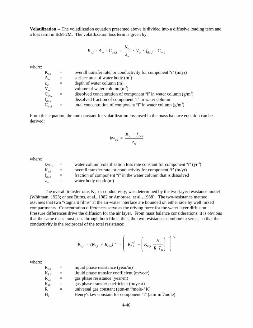
Kv,i � Aw � Cdw,i �Kv,i

zw

� Vw � fdw,i � Cwt,i

kwv,i �Kv,i � fdw,i

zw

Kv,i � (RL,i � RG,i)�1

� K �1L,i � KG,i

Hi

R TK

�1 �1

4-46

Volatilization -- The volatilization equation presented above is divided into a diffusive loading term anda loss term in IEM-2M. The volatilization loss term is given by:

where:K = overall transfer rate, or conductivity for component �i� (m/yr)v,i

A = surface area of water body (m )w2

z = depth of water column (m)w

V = volume of water column (m )w3

C = dissolved concentration of component �i� in water column (g/m )dw,i3

f = dissolved fraction of component �i� in water columndw,i

C = total concentration of component �i� in water column (g/m )wt,i3

From this equation, the rate constant for volatilization loss used in the mass balance equation can bederived:

where:kw = water column volatilization loss rate constant for component �i� (yr )v,i

-1

K = overall transfer rate, or conductivity for component �i� (m/yr)v,i

f = fraction of component �i� in the water column that is dissolveddw,i

z = water body depth (m)w

The overall transfer rate, K or conductivity, was determined by the two-layer resistance modelv,i

(Whitman, 1923; or see Burns, et al., 1982 or Ambrose, et al., 1988). The two-resistance methodassumes that two �stagnant films� at the air-water interface are bounded on either side by well mixedcompartments. Concentration differences serve as the driving force for the water layer diffusion. Pressure differences drive the diffusion for the air layer. From mass balance considerations, it is obviousthat the same mass must pass through both films; thus, the two resistances combine in series, so that theconductivity is the reciprocal of the total resistance:

where:R = liquid phase resistance (year/m)L,i

K = liquid phase transfer coefficient (m/year)L,i

R = gas phase resistance (year/m)G,i

K = gas phase transfer coefficient (m/year)G,i

R = universal gas constant (atm-m /mole-�K) 3

H = Henry's law constant for component "i" (atm-m /mole)i 3

Kv,i,T � Kv,i,20 � (T�20)

KL,i � u�

�a

�w

0.5k 0.33

�2

Sc�0.67w,i (3.15x107)

KG,i � u�k 0.33

�2

Sc�0.67a,i (3.15x107)

u�

� Cd0.5 W

Sca,i �µa

�a Da,i

�

�a

Da,i

4-47

T = water body temperature (�K)K

The value of K , the conductivity, depends on the intensity of turbulence in a water body and inv,i

the overlying atmosphere. As the Henry's Law constant increases, the conductivity tends to beincreasingly influenced by the intensity of turbulence in water. As the Henry's Law constant decreases,the value of the conductivity tends to be increasingly influenced by the intensity of atmosphericturbulence.

Because Henry's Law constant generally increases with increasing vapor pressure of a compoundand generally decreases with increasing solubility of a compound, highly volatile low solubilitycompounds are most likely to exhibit mass transfer limitations in water, and relatively nonvolatile highsolubility compounds are more likely to exhibit mass transfer limitations in the air. Volatilization isusually of relatively less magnitude in lakes and reservoirs than in rivers and streams.

The estimated volatilization rate constant was for a nominal temperature of 20 �C. It is adjustedfor the actual water temperature using the equation:

where:� = temperature correction factor, set to 1.026.T = water body temperature (�C)

There have been a variety of methods proposed to compute the liquid (K ) and gas phase (K )L,i G,i

transfer coefficients. For a stagnant system, the transfer coefficients are controlled by wind-inducedturbulence. For stagnant systems, the liquid film transfer coefficient (K ) is computed using theL,i

O'Connor (1983) equations:

where:

Da,i �1.9

MW2/3i

�a � (1.32 � 0.009 Ta) × 10�1

Scw,i �µw

�w Dw,i

Dw,i �22×10�5

MW2/3i

�w � 1 � 8.8×10�5 Tw

log(µw) �

1301

998.333� 8.1855(Tw�20) � 0.00585(Tw�20)2� 3.0233

4-48

and:u = shear velocity (m/s)*

C = drag coefficient (= 0.0011)d

W = wind velocity, 10 m above water surface (m/s)� = density of air corresponding to the air temperature (g/cm )a

3

� = density of water corresponding to the water temperature (g/cm )w 3

k = von Karman's constant (= 0.4)� = dimensionless viscous sublayer thickness (= 4)2

Sc = air Schmidt number for component "i" (dimensionless)a,i

Sc = water Schmidt number for component "i" (dimensionless)w,i

D = diffusivity of component "i" in air (cm /sec)a,i 2

D = diffusivity of component "i" in water (cm /sec)w,i 2

µ = viscosity of air corresponding to the air temperature (g/cm-s)a

µ = viscosity of water corresponding to the water temperature (g/cm-s)w

� = dynamic viscosity of air (cm /sec)a2

MW = molecular weight of component "i"i

T = air temperature (�C)a

T = water temperature (�C)w

3.15x10 = units conversion factor (sec/yr)7

volume iii: fate and transport of mercury … · volume iii: fate and transport of mercury in the...

Documents