Naval Research Laboratory Washington, DC 20375-5320

NRL/MR/7600--15-9640

Volume 4.NRL SSD Research Achievements: 1990–2000

October 30, 2015

Approved for public release; distribution is unlimited.

Jill Dahlburg george Doschek kenneth DymonD stephen eckermann Douglas Drob John emmert christoph englert russell howarD w. neil Johnson clarence korenDyke michael lovellette DaviD siskinD Dennis socker michael stevens michael wolff kent wooD

Space Science Division

i

REPORT DOCUMENTATION PAGE Form ApprovedOMB No. 0704-0188

3. DATES COVERED (From - To)

Standard Form 298 (Rev. 8-98)Prescribed by ANSI Std. Z39.18

Public reporting burden for this collection of information is estimated to average 1 hour per response, including the time for reviewing instructions, searching existing data sources, gathering and maintaining the data needed, and completing and reviewing this collection of information. Send comments regarding this burden estimate or any other aspect of this collection of information, including suggestions for reducing this burden to Department of Defense, Washington Headquarters Services, Directorate for Information Operations and Reports (0704-0188), 1215 Jefferson Davis Highway, Suite 1204, Arlington, VA 22202-4302. Respondents should be aware that notwithstanding any other provision of law, no person shall be subject to any penalty for failing to comply with a collection of information if it does not display a currently valid OMB control number. PLEASE DO NOT RETURN YOUR FORM TO THE ABOVE ADDRESS.

5a. CONTRACT NUMBER

5b. GRANT NUMBER

5c. PROGRAM ELEMENT NUMBER

5d. PROJECT NUMBER

5e. TASK NUMBER

5f. WORK UNIT NUMBER

2. REPORT TYPE1. REPORT DATE (DD-MM-YYYY)

4. TITLE AND SUBTITLE

6. AUTHOR(S)

8. PERFORMING ORGANIZATION REPORT NUMBER

7. PERFORMING ORGANIZATION NAME(S) AND ADDRESS(ES)

10. SPONSOR / MONITOR’S ACRONYM(S)9. SPONSORING / MONITORING AGENCY NAME(S) AND ADDRESS(ES)

11. SPONSOR / MONITOR’S REPORT NUMBER(S)

12. DISTRIBUTION / AVAILABILITY STATEMENT

13. SUPPLEMENTARY NOTES

14. ABSTRACT

15. SUBJECT TERMS

16. SECURITY CLASSIFICATION OF:

a. REPORT

19a. NAME OF RESPONSIBLE PERSON

19b. TELEPHONE NUMBER (include areacode)

b. ABSTRACT c. THIS PAGE

18. NUMBEROF PAGES

17. LIMITATIONOF ABSTRACT

Volume 4. NRL SSD Research Achievements: 1990–2000

Jill Dahlburg, George Doschek, Kenneth Dymond, Stephen Eckermann, Douglas Drob,John Emmert, Christoph Englert, Russell Howard, W. Neil Johnson, Clarence Korendyke, Michael Lovellette, David Siskind, Dennis Socker, Michael Stevens, Michael Wolff,and Kent Wood

Naval Research Laboratory4555 Overlook Avenue, SWWashington, DC 20375-5320 NRL/MR/7600--15-9640

NRL

Approved for public release; distribution is unlimited.

UnclassifiedUnlimitedUnclassified

UnlimitedUnclassifiedUnlimited

UnclassifiedUnlimited

93

Jill Dahlburg

(202) 767-6343

The 1990s saw the deployment and execution of myriad Naval Research Laboratory (NRL) Space Science Division (SSD) experiments into space. This summary provides a technical overview of some of the major NRL SSD research achievements during this decade, 1990-2000.

30-10-2015 Memorandum Report

Space Science History

1990 – 2000

Naval Research Laboratory4555 Overlook Avenue, SWWashington, DC 20375-5320

ii

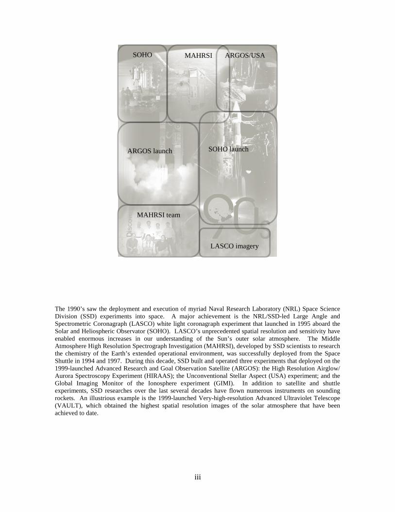
The 1990’s saw the deployment and execution of myriad Naval Research Laboratory (NRL) Space Science Division (SSD) experiments into space. A major achievement is the NRL/SSD-led Large Angle and Spectrometric Coronagraph (LASCO) white light coronagraph experiment that launched in 1995 aboard the Solar and Heliospheric Observator (SOHO). LASCO’s unprecedented spatial resolution and sensitivity have enabled enormous increases in our understanding of the Sun’s outer solar atmosphere. The Middle Atmosphere High Resolution Spectrograph Investigation (MAHRSI), developed by SSD scientists to research the chemistry of the Earth’s extended operational environment, was successfully deployed from the Space Shuttle in 1994 and 1997. During this decade, SSD built and operated three experiments that deployed on the 1999-launched Advanced Research and Goal Observation Satellite (ARGOS): the High Resolution Airglow/ Aurora Spectroscopy Experiment (HIRAAS); the Unconventional Stellar Aspect (USA) experiment; and the Global Imaging Monitor of the Ionosphere experiment (GIMI). In addition to satellite and shuttle experiments, SSD researches over the last several decades have flown numerous instruments on sounding rockets. An illustrious example is the 1999-launched Very-high-resolution Advanced Ultraviolet Telescope (VAULT), which obtained the highest spatial resolution images of the solar atmosphere that have been achieved to date.

MAHRSI team

ARGOS launch

SOHO

SOHO launch

LASCO imagery

MAHRSI ARGOS/USA

iii

PREFACE We offer these summaries of Naval Research Laboratory (NRL) Space Science Division (SSD) research achievements to provide a technical overview of NRL space science accomplishments from the beginning of the Division in 1952 through the first decade of the 21st century. These summaries are presented in five Volumes: Volume 1. NRL SSD Research Achievements: 1960-1970 Volume 2. NRL SSD Research Achievements: 1970-1980 Volume 3. NRL SSD Research Achievements: 1980-1990 Volume 4. NRL SSD Research Achievements: 1990-2000 Volume 5. NRL SSD Research Achievements: 2000-2010 The importance of space science basic research in support of naval needs was robustly championed by Homer Newell, the Division's second Superintendent, who noted to the US Congress in 1957, "A strong basic research program is essential to continuing vitality of applied R&D in missiles or any other military or peacetime applications. New facts, new ideas, new techniques, new materials, new instruments, all come from the basic research effort..." As the dozens of summaries in these five Volumes tremendously attest, extraordinary ranges of research and results have been achieved. To document significant SSD historical accomplishments, Drs. George Doschek and Jill Dahlburg requested current and former SSD researchers to contribute technical achievement summaries to these Volumes on the basis of their personal memories about the scientific activities in which they were involved. The contributions received were then loosely organized by decade into these five featured Volumes, after being edited for clarity by George Doschek, Tanisha Lucas, and Jill Dahlburg. George Doschek would like to express his gratitude to all the researchers who have contributed to these summaries, and particularly to those with whom he has personally worked. The SSD has and is currently continuing to provide substantive and significant contributions to the developments of experimental space science since its origins after World War II, and it has been a privilege to be part of this effort. These Volumes convey stories about curiosity, hopes, and aspirations of scientists fascinated by exploration of the Universe with instrumentation placed beyond the Earth's atmosphere. Tanisha Lucas wishes to acknowledge that she has benefited from the advice, assistance, and all of the contributions that our researchers put into these documents. She wishes to express her gratitude to the NRL SSD researchers for their remarkable scientific contributions, her appreciation for the advice on content and organization for this book provided by Dr. Jill Dahlburg, and her many thanks to Dr. George Doschek for closely working with her in compiling and arranging these Volumes. Jill Dahlburg acknowledges with pleasure and gratitude the request from Dr. John Montgomery, NRL Director of Research, that these Volumes be developed. They present a unique account of exceptional contributions from the NRL SSD broad-spectrum research, development and experimentation program to study the atmospheres of the Sun and the Earth, the physics and properties of high-energy space environments, and solar activity and its effects on the Earth’s atmosphere, and to transition these capabilities to operational use. Finally, George, Tanisha and Jill would together like to thank Ms. Kathryn Grouss who worked with us to prepare these Volumes during 2014, for her exceptional cooperation, professionalism, assistance and advice, and to Dr. Angelina Callahan, NRL Associate Historian, for her many beneficial insights and suggestions, and her unswerving encouragement. George Doschek, NRL SSD Historian Tanisha Lucas, NRL SSD Research Achievements Managing Editor Jill Dahlburg, NRL SSD Superintendent ____________________________ Manuscript approved December 22, 2014.

iv

1

Table of Contents Decadal Image .......................................................................................................................................... ii Image Description .................................................................................................................................... iii Preface ....................................................................................................................................................... iv Overview of the NRL Space Science Division 1990’s Decade ................................................................. 03 90’s.1: The Large Angle Spectroscopic Coronagraph (LASCO) on the Solar and Heliospheric Observatory (SOHO) - Contributed by George A. Doschek & Russell A. Howard ....................... 04

1.0 Historical Perspective ............................................................................................................................ 04 2.0 The SOHO spacecraft............................................................................................................................ 05 3.0 The LASCO instruments ....................................................................................................................... 06 4.0 Scientific Results from LASCO ............................................................................................................ 08

90’s.2: Middle Atmosphere High Resolution Spectrograph Investigation (MAHRSI)- Contributed by David E. Siskind, Michael Stevens, and Robert R. Meier .......................................................... 13

1.0 Introduction ........................................................................................................................................... 13 2.0 Instrument and Observational Approach ............................................................................................... 13 3.0 Legacy of MAHRSI .............................................................................................................................. 15

90’s.3I: ARGOS PART I: SSD Experiments on ARGOS – Overview- Contributed by Kent S. Wood, Michael Lovellette, and Kenneth Dymond ......................................................................... 18

1.0 Introduction ........................................................................................................................................... 18 2.0 ARGOS Mission and the ARGOS Experiments Office ........................................................................ 18 3.0 Design Coordination to Meet ARGOS Specifications; the Gimbal Issue ............................................. 20 4.0 Coordination of Procurements............................................................................................................... 20 5.0 Construction Phase, Problem Resolution, Testing ................................................................................ 20 6.0 Summary ............................................................................................................................................... 22

90’s.3II: ARGOS PART II: The USA Experiment- Contributed by Kent S. Wood and Michael Lovellette ..................................................................................................................................... 23

1.0 Introduction ........................................................................................................................................... 23 2.0 Research Program: Four Research Thrusts ........................................................................................... 23 3.0 Experiment Development: Tailoring USA to the Four Research Themes ............................................ 26 4.0 ARGOS Flight and Results ................................................................................................................... 27 5.0 Aftermath and Legacy ........................................................................................................................... 33

90’s.3III: ARGOS Part III: The High Resolution Airglow and Aurora Spectroscopy (HIRAAS) Experiment for ARGOS- Contributed by Kenneth F. Dymond.................................................. 36

1.0 Introduction ........................................................................................................................................... 36 2.0 Instrument Descriptions ........................................................................................................................ 37 3.0 HIRAAS Program ................................................................................................................................. 39 4.0 Key Scientific and Technical Results .................................................................................................... 40 5.0 Key Personnel ....................................................................................................................................... 46 6.0 Legacy ................................................................................................................................................... 46

90’s.3IV: ARGOS PART IV: The Global Imaging Monitor of the Ionosphere (GIMI) Experiment- Contributed by Michael T. Wolff and Kenneth F. Dymond ........................................................ 49

1.0 Introduction ........................................................................................................................................... 49 2.0 Program Background............................................................................................................................. 49 3.0 Science Objectives ................................................................................................................................ 49 4.0 The GIMI Instrument ............................................................................................................................ 50 5.0 Key Experiment Results ........................................................................................................................ 52 6.0 Legacy ................................................................................................................................................... 54

2

90’s.4: EUV Solar Physics sounding rockets at NRL (1975-2005)- Contributed by Clarence M. Korendyke....................................................................................................................................... 56

1.0 Overview ............................................................................................................................................... 56 2.0 HRTS sounding rocket program............................................................................................................ 57 2.1 The First Rocket Flight: July 21, 1975 .................................................................................................. 60 2.2 The Second Rocket Flight: February 13, 1978 ...................................................................................... 60 2.3 The Third Rocket Flight: March 1, 1979 ............................................................................................... 60 2.4 The Fourth Rocket Flight: March 7, 1983 ............................................................................................. 61 2.5 The Fifth HRTS Rocket Flight: December 11, 1987............................................................................. 61 2.6 The Sixth Rocket Flight: November 20, 1988 ....................................................................................... 61 2.7 The Seventh Rocket Flight: November 21, 1990 .................................................................................. 62 2.8 The Eighth Rocket Flight: August 24, 1992 .......................................................................................... 62 2.9 The Ninth Rocket Flight: April 18, 1995 ............................................................................................. 63 2.10 The Tenth Rocket Flight: September 30, 1997 .................................................................................. 64 3.0 The VAULT Instrument ........................................................................................................................ 65 4.0 Field Operations .................................................................................................................................... 66

90’s.5: The Mountain Wave Forecast Model (MWFM)- Contribute by Stephen D. Eckermann .............. 71

1.0 Introduction ........................................................................................................................................... 71 2.0 Meeting the Science Challenge: the Mountain Wave Forecast Model (MWFM) ................................. 71 3.0 Exploiting the Potential: MWFM-2 ...................................................................................................... 72 4.0 Sudden DoD Relevance: 11 September 2001........................................................................................ 75 5.0 The Future: MWFM-3, State-of-the-Art Ray Methods and Next-Generation Prediction ..................... 76

90’s.6: Space Science Division (SSD) Upper Atmospheric Empirical Modeling- Contributed by John Emmert, Douglas Drob, Michael Picone, and Robert Meier ................................................ 79

1.0 Introduction ........................................................................................................................................... 79 2.0 Empirical modeling heritage in SSD ..................................................................................................... 79 3.0 Scientific and Operational Legacy ........................................................................................................ 83

A1. List of Terms and Acronyms ............................................................................................................... 85

3

Overview of the NRL Space Science Division 1990’s Decade At the US Naval Research Laboratory (NRL), the story of space research formally began in 1952, with the creation of the NRL Atmospheres and Astrophysics (A&A) Division under the direction of Dr. John Hagen, and a Division charter to perform research and development in the field of space science. The Division’s second Superintendent, Homer Newell (1956-1958), continued A&A’s seminal space research both at NRL and then later at the National Aeronautics and Space Administration (NASA). Following Dr. Newell’s departure to NASA in 1958, Herbert Friedman assumed leadership of NRL space science as the third A&A Division Superintendent (1958-1982). Dr. Friedman oversaw the renaming of the Division from A&A to Space Science, in 1968, and in 1982 he transitioned the Division to the leadership of Dr. Herbert Gursky, who served as SSD’s fourth Superintendent from 1982-2006. Jill Dahlburg, the fifth and current SSD Superintendent, was appointed to the position in 2007 following her service as Acting SSD Superintendent from May 2006. The scope of the NRL Space Science Division encompasses theoretical, experimental and numerical research of geophysics science and technology, solar and heliospheric physics, and the high-energy space environment, and the conception, design, fabrication, integration, test, operation and experimentation with forefront space instrumentation, for the purpose of enabling Navy/ Marine Corps and wider DoD robust access to space assets. The 1990’s saw the deployment and execution of myriad Naval Research Laboratory (NRL) Space Science Division (SSD) experiments into space. During this decade, the Division was deeply involved in scientific experiments on the 1999-launched Advanced Research and Global Observation Satellite (ARGOS), three of which experiments were built and operated by SSD scientists: the High Resolution Airglow/Aurora Spectrograph experiment (HIRAAS); the Unconventional Stellar Aspect (USA) experiment; and, the Global Imaging Monitor of the Ionosphere experiment (GIMI). These instruments, which involved many forefront research areas -- including X-ray astrophysics, X-ray navigation and aeronomy, reliable computing in space, and ultraviolet/extreme-ultraviolet (UV/EUV) spectroscopy and imaging of the Earth’s atmosphere -- are overviewed in Essay 90’s.3. In the area of geophysics science and technology a breadth of basic and applied research was advanced in addition to the ARGOS experiments noted above. NRL’s Middle Atmosphere High Resolution Spectrograph Investigation (MAHRSI), developed by SSD scientists to research the chemistry of the Earth’s extended operational environment, was successfully fielded from the space shuttle in 1994 and 1997 as summarized in Essay 90’s.2. The Mountain Wave Forecast Model (MWFM), described in Essay 90’s.5, forecasts clear-air turbulence in the stratosphere above mountains; the MWFM, which was largely developed in the 1990’s, was used during Southern Watch, Enduring Freedom, and Iraqi Freedom to predict flight conditions for allied aircraft during these operations. The SSD upper atmospheric empirical modeling program, overviewed in Essay 90’s.6, is another important and high-impact upper atmosphere research program that continues today, and which has to-date contributed a wide range of useful capabilities such as the NRLMSISE-00 model. In NRL SSD 1990’s solar and heliospheric physics research, a major achievement is the NRL SSD-led Large Angle and Spectrometric Coronagraph (LASCO) white light coronagraph experiment that launched in 1995 aboard the Solar and Heliospheric Observatory (SOHO). LASCO continues to provide a real-time eye on our Sun from the L1 Lagrangian point, gathering enormous quantities of valuable data about coronal mass ejections and other physical processes that occur in the solar atmosphere. As described in Essay 90’s.1, LASCO’s unprecedented spatial resolution, sensitivity, and reliability are enabling tremendous increases in our understanding of geoeffective solar storms. And, rounding out the extraordinary achievements of this decade, Essay 90’s.4 provides a summary of exciting, ongoing SSD sounding rocket research. In addition to satellite and shuttle experiments, over the last several decades SSD researchers have developed and fielded numerous solar instrument experiments on sounding rockets to test new concepts and gather first-of-a-kind space data. A particularly innovative SSD rocket concept was the High Resolution Telescope and Spectrograph (HRTS) that obtained the first arc-second spatial and spectral resolution observations of the lower transition region of the Sun’s atmosphere. HRTS also served as a steppingstone to even higher spatial-resolution observations, such as that demonstrated on the 1999-launched Very-high-resolution Advanced ULtraviolet Telescope (VAULT), which achieved sub-arc-second resolution images of the solar atmosphere’s chromosphere/transition region.

4

90’s.1: The Large Angle Spectroscopic Coronagraph (LASCO) on the Solar and Heliospheric Observatory (SOHO)

Contributed by George A. Doschek and Russell A. Howard

1.0 Historical Perspective The study of the solar corona using space-borne white light coronagraphs was begun by SSD’s Dr. Richard Tousey and his Rocket Spectroscopy Branch beginning in the early 1960’s using sounding rockets flown from White Sands, New Mexico. This program led to the NRL coronagraph on the NASA Seventh Orbiting Solar Observatory (OSO-7), launched in 1971 and the discovery at NRL of coronal mass ejections (CMEs) (see OSO essay 60s.2). However, NRL had stiff competition from the High Altitude Observatory (HAO) in Boulder, Colorado in fielding space-borne coronagraphs. The HAO coronagraph on the Skylab manned space station, launched in 1973, used film and obtained beautiful high spatial resolution images of CMEs, and the HAO group was very strong scientifically and also published prolifically. NRL followed the HAO achievement with the coronagraph on P78-1, launched in 1979, and was equally prolific in publications. The P78-1 science results were quite comprehensive (see P78-1 essay 70s.3). HAO followed this with a coronagraph on the NASA Solar Maximum Mission (SMM), launched in 1980, and also produced new and comprehensive results. Then NRL and HAO teamed to develop the imaging instrument, a combination white light coronagraph, X-Ray and extreme-ultraviolet (EUV) telescope for the NASA/ESA Out-of-the-Ecliptic (OOE) Mission. The U.S. spacecraft, which had the imaging instrument, was canceled in 1982. The ESA spacecraft continued and was renamed Ulysses after its launch in 1990. Which of these two experimentally experienced and scientifically strong coronagraph groups would produce the next space coronagraph and on what mission would it fly? Years passed before this question was answered. In 1979, the NRL/SSD Rocket Spectroscopy Branch was dissolved and solar research was reformed into two solar oriented Branches: Code 7660, the Solar Physics Branch led by Dr. Guenter Brueckner, and Code 7670, the Solar-Terrestrial Relationships Branch led by Dr. George Doschek. Code 7660 was the follow-on of the Rocket Spectroscopy Branch and Code 7670 was a new Branch. The population of these Branches was from the Rocket Spectroscopy Branch and the X-ray solar group in Talbot Chubb’s Upper Air Physics Branch. The coronagraph group was placed in Code 7670. After OOE, there was a period in which no new solar mission suitable for a coronagraph appeared on the horizon; during this time, both the SMM and P78-1 coronagraphs continued to operate and yielded good results. It was as if new opportunities for coronal research via coronagraphs were now finished. However, because of the importance of coronagraph results to operations, the coronagraph group (a section in Code 7670) lead by NRL’s Dr. Donald Michels was kept intact in spite of a lack of immediate new missions. The group obtained NRL basic research funding and funds from NASA grants for other activities, and attempted to play a major role in other solar space missions. For example, Don Michels and his section produced a proposal for the soft X-ray telescope (SXT) on the Japanese Solar-A mission (Yohkoh), and Don Michels served on an international working group that helped define the characteristics of the Yohkoh spacecraft. In 1982, ESA began the formulation of a science program of missions for the next decade. Included in the options was a heliospheric mission which would include a space-based helioseismology experiment. In 1983, ESA sponsored a study to define the mission concept which

5

became the Solar & Heliospheric Observatory (SOHO) mission. Don Michels participated in the mission concept, to study the solar interior, the outer solar corona, and the solar wind. ESA submitted the concept in November, 1982 to the Science Policy Committee, which approved the program as one element of the Cornerstone 2000 program. The call for proposals came out in March. The origin of the Large Angle Spectroscopic Coronagraph (LASCO) began as Don Michels and the scientists in his NRL section (Russell Howard, Martin Koomen, and Neil Sheeley) considered how to respond to the possible opportunity to fly a coronagraph on SOHO. Don and his group had already established a collaboration with Dr. Rainer Schwenn at the institute now called the Max Planck Institute for Solar System Research (MPS) in Katlenburg-Lindau, Germany. They also discussed the opportunity with the HAO for potential competition and initially they agreed to collaborate and not compete as they did for the OOE proposal. However, Don’s group was interested in exploring the region of interplanetary space beyond the 10 solar radii reach of the Solar Wind (SOLWIND) coronagraph on P78-1, while HAO thought it best to attempt to reduce the occulting disk and observe coronal features as close to the solar disk as possible. Both objectives have high scientific value. HAO finally decided to pull out of the collaboration and compete. In NRL/SSD it was decided that the size of the entire coronagraph field-of-view (FOV) could not be accommodated with a single coronagraph. To summarize briefly, the final proposed NRL-led instrument contains an inner coronagraph (C1) that operates between 1.1 and 3 solar radii, provided by MPS, a middle coronagraph (C2) that operates between 1.5 and 6 solar radii, provided by the Laboratoire d’Astronomie Spatiale, Marseille, France, and an outer coronagraph (C3) that operates between 3.7 and 30 solar radii, provided by SSD. In addition, Code 7660 was brought into the program and they provided a high-resolution imaging spectrometer/Fabry-Perot interferometer for the C1 coronagraph; this instrument is described in detail by Brueckner et al. (1995). The NRL/SSD coronagraph was proposed by Code 7670 in a NASA proposal competition, and accepted for flight with Don Michels as the Principal Investigator. The U.S. Project Scientist was Russell Howard, and the Project Scientist for Europe and Co-Ordinator for West Germany was Rainer Schwenn, the Co-Ordinator for France was Dr. Philippe Lamy from the Laboratoire d’Astronomie Spatiale. Some time after acceptance NASA decided that cost reductions should be made in all the US instruments, and SSD began a collaboration with Professor George Simnett at the University of Birmingham in the UK. They agreed to provide the aluminum structure that would house all the coronagraphs. This cut US costs and satisfied the NASA cost reduction requirement. The coronagraph suite proved to be more of a challenge than anticipated due to the international partners, the necessity of satisfying both NASA and ESA requirements and the large inter-Branch dependencies. It was decided to appoint Guenter Brueckner, the head of the Code 7660 Branch who had much experience with NASA programs, to be the PI, and to make Don Michels the Program Scientist, with primary responsibility to interface with the international partners. The two Codes normally functioned in a complementary fashion, and NRL regarded both branches as forming a single NRL solar physics and solar terrestrial physics program. Under Brueckner’s experienced and outstanding leadership, and the excellent technical expertise from Don Michels and his section, a superb LASCO instrument was built and delivered to NASA. From this Brueckner was able to convince the NRL Director of Research, Dr. Timothy Coffey, that a new coronagraph test building was needed as well as other space within SSD. 2.0 The SOHO spacecraft The SOHO spacecraft was placed at the L1 Lagrangian point, along the Sun-Earth line and about 1 million miles from Earth. The spacecraft was built by a European industrial consortium lead by the company now called Airbus Defense and Space and was launched on a Lockheed-Martin Atlas II

6

on 2 December 1995. SOHO began standard operations in May 1996. Although originally planned as a two-year mission, SOHO continues to operate to this day with LASCO observing about 14,000 CMEs by mid-2009. The SOHO operation center is at Goddard Space Flight Center. Because SOHO is at the L1 point in space, the overall data rate is not large enough for optimal study of highly transient dynamical studies of flares, etc. After launch, additional telemetry was found from unused packets and allocated to LASCO/EIT. Therefore, SOHO’s main objectives concern the so-called quiet Sun, although it is also highly dynamical. In June 1998 SOHO suffered a mishap and the instruments were shut down. Recovery was difficult and heroic, but success was achieved and by the end of October the instruments were functioning again although some suffered problems due to the long deep freeze. The C1 interferometer was no longer operative. However, overall LASCO continues to operate normally to this day and continues to produce exceptionally fine coronal images routinely. The spacecraft and instruments are shown in Figure 90s.1.1.

Figure 90s.1.1 – Left: The SOHO spacecraft; right: the SOHO payload (credit: NASA/ESA/NRL). 3.0 The LASCO instruments The C1 coronagraph is a mirror version of the classic internally occulted Lyot coronagraph, while the C2 and C3 instruments are externally occulted coronagraphs. The reader is referred to Brueckner et al. (1995) for a detailed discussion of their operation, which reference has, as of this writing, about 1500 citations. Figure 90s.1.2 illustrates the optical complexity of the coronagraphs and the baffling necessary to reduce stray and scattered light. The coronagraphs measure the Thomson-scattered light from the solar disk, but this radiation is orders of magnitude fainter than the solar disk. Suppressing scattered light is absolutely essential at all solar radii above the disk, and it is even more crucial at the large distances greater than 10 solar radii.

7

Figure 90s.1.2 – Schematic diagram of the LASCO C2 coronagraph (from Brueckner et al. 1995) (Figure 10 in Brueckner et al. 1995, courtesy Solar Physics). The LASCO detectors consisted of three cameras, and in addition, LASCO provided the electronics and the CCD camera for another SOHO instrument, the Extreme-ultraviolet Imaging Telescope (EIT). EIT provides full-disk observations in four narrow wavelength bands produced by coating four segments of the EIT mirror with different multilayer coatings (see Delaboudiniere et al. 1995 for details). The EIT camera is linked to the LASCO electronics such that LASCO sees the EIT camera simply as a fourth camera. The data read-outs of LASCO and EIT are linked together. SSD personnel made large contributions to the development of the EIT instrument, led by J.-P. Delaboudiniere from the Institute d’Astrophysique Spatiale, University of Paris. The performance of LASCO has been outstanding and has established NRL/SSD as the world’s leading group for producing solar coronagraphs. The performance and use of LASCO by the global solar community helped SSD to archive the NASA Solar Terrestrial Relations Observatory (STEREO) opportunity and to having coronagraphs on both the ESA Solar Orbiter mission and the NASA Solar Probe Plus mission. The importance of LASCO for the solar program in the US cannot be underestimated. Figure 90s.1.3 illustrates the beauty of the LASCO images and the outstanding achievement in suppressing stray light levels. Note that there is a strong stellar background and the presence of a sungrazing comet in the image (see section 4.6 for more about comets).

8

Figure 90s.1.3 – A C3 coronagraph image illustrating the large spatial field-of-view of LASCO. The white circle at the center of the image is an outline to scale of the occulted Sun. The occulter and its support arm are clearly visible. Coronal streamers are seen on the east and west solar limbs, and a portion of the Milky Way is visible in the bottom part of the image. The streak near the occulter support arm is a comet (credit: NASA/NRL). 4.0 Scientific Results from LASCO LASCO has observed the Sun continuously from 1995 to the present and into the forseeable future, and so a large database is now in hand for determining basic properties of the corona and activity such as coronal mass ejections over both solar minimum and solar maximum parts of the solar cycle. This information is crucial for space weather applications. In addition, with LASCO many small-scale coronal events have been discovered which shed light on basic processes in the corona such as magnetic reconnection. And finally, LASCO has discovered more than 2500 comets as of November 2013 (e.g., see Figure 90s.1.3), which is a substantial fraction of all comets discovered by other means. Below are brief summaries of some of the LASCO scientific highlights. 4.1 Discovery of coronal outflows: Early in the data analysis, inhomogeneous structures were seen in the coronal images (see Figure 90s.1.4) that passively trace the outflow of the slow solar wind (e.g., Sheeley et al. 1997; Sheeley et al. 1999). The sizes, speeds, and accelerations were measured, providing new insight into the detailed structure of the outer solar corona. These small density enhancements were postulated to be the result of interchange reconnection, occurring at the tops of the helmet streamer arcade, and enabling the release of material previously trapped.

9

Figure 90s.1.4 – Running difference LASCO images showing outflowing blobs. Each blob is moving within a streamer and has white/dark components due to the running differences. The white regions are the leading edges of the outflows (Figure 1 in Sheeley et al. 1997, reproduced by permission of the AAS) . 4.2 Discovery of coronal inflows and in-out pairs: In addition to purely outflowing plasma, structures were found that consist of two components, one that moves outward while the other moves back towards the Sun (e.g., Wang et al. 1999; Sheeley & Wang 2002; Sheeley & Wang 2007). Studies of many such events show that they represent a broad class of streamer detachments, including streamer blowout CMEs. It is believed that the in-out pairs occur when rising magnetic loops reconnect to form an outward helical flux rope and an inflowing arcade of collapsing loops. Such observations are direct evidence of magnetic reconnection in the solar corona (see Figure 90s.1.5).

Figure 90s.1.5 – Running difference LASCO images of in-out pairs indicated by arrows (Figure 14 in Sheeley & Wang 2002, reproduced by permission from the AAS).

10

4.3 Properties of CMEs Over a Solar Cycle: An extensive catalogue of CMEs has been prepared from the LASCO images obtained from the time SOHO science operations began. By mid-2009 the catalogue contained 14,000 entries and is the largest collection of CME properties readily available on-line (Vourlidas et al. 2010). The measured properties of CMEs include masses, energies, speeds, densities, shapes, sizes, acceleration characteristics, and relationship to the solar cycle and other heliophysics phenomena. From these observations, as exemplified in Figure 90s.1.6, we are finally beginning to understand the physics of CME origin, propagation, and interactions with the existing solar atmosphere (e.g., Zhang et al. 2004; Yashiro et al. 2004; Vourlidas et al. 2010).

Figure 90s.1.6 – Left: A LASCO CME with an EIT image superimposed on the occulting disk (credit: NASA/NRL). Right: Distributions of mass and energy based on the LASCO catalogue (Figure 8 in Vourlidas et al. 2010, reproduced by permission of the AAS). 4.4 Identification of the Structure of CMEs as a Magnetic Flux Rope: One of the crowning achievements based on LASCO is the identification of mass ejections as a magnetic flux rope. The various orientations of CMEs in the plane of the sky and their diversity in directions of travel give CMEs many apparent shapes based on view angle. Untangling these shapes and identifying a few basic CME structures was one of the primary goals of LASCO, with its large field of view and high sensitivity. The magnetic flux rope is a common CME structure (e.g., Chen et al. 1997; Wood et al. 1999; Chen et al. 2000; Krall et al. 2001). This is not immediately obvious by looking at the majority of CMEs. 4.5 Confirmation of the Importance of Halo CMEs for Space Weather: Some CMEs are Earth-directed. They can look like vast halos that surround the Sun (see Figure 90s.1.7). Extensive studies of these Earth-directed CMEs based on LASCO observations have confirmed their geoeffectiveness in producing adverse space weather phenomena (e.g., Vourlidas et al. 2003; Zhang et al. 2003; Gopalswamy et al. 2005a,b). Predicting space weather events is of prime importance not only for the protection of DoD space assets, but is also important in many other business enterprises, e.g., power companies, airline industries, NASA manned space program. These studies continue to be made by combining LASCO data with data from the NASA STEREO mission (see 2000s chapter Essay 2000s.3). The combination of LASCO and STEREO observations gives views of CMEs from three different positions in the heliosphere, allowing their shapes and heliospheric interactions to be determined.

11

Figure 90s.1.7 – A running difference image of a LASCO partial halo CME. This shows the enormous size of CMEs (credit: NRL). 4.6 Discoveries of Comets: Sungrazing comets from space observations were discovered by the NRL SOLWIND coronagraph on P78-1 (see P78-1 Essay 70’s.3). LASCO images reveal many sungrazing comets, large and small, as they near the Sun and pass into the LASCO field-of-view (e.g., Biesecker et al. 2002). As of October 2013, over 2,600 comets have been discovered, which makes LASCO the most prolific discoverer of comets in history. The LASCO data are available to anyone who wishes to search for comets. Thus LASCO is a terrific public outreach instrument and people in many different professions, some far from science, have discovered comets in LASCO data. This database of comets is a valuable resource to comet researchers for understanding the evolution of comet groups and for determining the physical characteristics of comets. A spectacular example of a LASCO comet is shown in Figure 90s.1.8. Many comets are not nearly this spectacular and require patience and diligence to detect them. This makes the search for sungrazer comets that much more exciting.

Figure 90s.1.8 – A LASCO sungrazer comet (at “8 o’clock”) in its approach towards perihelion (credit: NASA/NRL).

12

References: 90s.1: The Large Angle Spectroscopic Coronagraph (LASCO) on the Solar & Heliospheric Observatory (SOHO) Biesecker, D. A., Lamy, P., St. Cyr, O. C., Llebaria, A., & Howard, R. A. 2002, Icarus, 157, 323 Brueckner, G. E. et al. 1995, Sol. Phys., 162, 357 Chen, J. et al. 1997, Astrophys. J., 490, L191 Chen, J. et al. 2000, Astrophys. J., 533, 481 Delaboudiniere, J.-P. et al. 1995, Sol. Phys., 162, 291 Gopalswamy, N., Lara, A., Manoharan, P. K., & Howard, R. A. 2005a, Advances in Space Research, 36, 2289 Gopalswamy, N., Yashiro, S., Michalek, G., Xie, H., Lepping, R. P., & Howard, R. A. 2005b, Geophys. Res. Letters, 32, L12S09 Krall, J., Chen, J., Duffin, R. T., Howard, R. A., & Thompson, B. J. 2001, Astrophys. J., 562, 1045 Sheeley, Jr., N. R. et al. 1997, Astrophys. J., 484, 472 Sheeley, Jr., N. R., Walters, J. H., Wang, Y.-M., & Howard, R. A. 1999, J. Geophys. Res., 104, 24,739 Sheeley, Jr., N. R., & Wang, Y.-M. 2002, Astrophys. J., 579, 874 Sheeley, Jr., N. R., & Wang, Y.-M. 2007, Astrophys. J., 655, 1142 Vourlidas, A., Howard, R. A., Esfandiari, E., Patsourakos, S., Yashiro, S., & Michalek, G. 2010, Astrophys. J., 722, 1522 Vourlidas, A., Wu, S. T., Wang, A. H., Subramanian, P., & Howard, R. A. 2003, Astrophys. J., 598, 1392 Wang, Y.-M., Sheeley, Jr., N. R., Howard, R. A., St. Cyr, O. C., & Simnett, G. M. 1999, Geophys. Res. Letters, 26, 1203 Wood, B. E., Karovska, M., Chen, J., Brueckner, G. E., Cook, J. W., & Howard, R. A. 1999, Astrophys. J., 512, 484 Yashiro, S., Gopalswamy, N., Michalek, G., St. Cyr, O. C., Plunkett, S. P., Rich, N. B., & Howard, R. A. 2004, J. Geophys. Res., 109, A07105 Zhang, J., Dere, K. P., Howard, R. A., & Bothmer, V. 2003, Astrophys. J., 582, 520 Zhang, J., Dere, K. P., Howard, R. A., & Vourlidas, A. 2004, Astrophys. J., 604, 420

13

90’s.2: Middle Atmosphere High Resolution Spectrograph Investigation (MAHRSI)

Contributed by David E. Siskind, Michael Stevens,

and Robert R. Meier (retired from NRL)

1.0 Introduction The SSD Middle Atmosphere Program (MAP) commenced in the early 1980’s. At that time, the altitude and geographic distribution of the hydroxyl radical (OH), one of the principal carriers of chemical energy in the stratosphere and mesosphere, was essentially unknown. This trace constituent held the key to validating our understanding of water and other middle atmosphere species, and their interactions with sunlight. The only credible measurement was a single sounding rocket experiment more than a decade earlier. MAP, first led by SSD’s Donald Anderson and then by SSD’s Robert Conway quickly identified the measurement and modeling of OH in the middle atmosphere as one of its main science objectives. The major impediment to carrying out a spectrographic measurement of OH was the large brightness of Rayleigh-scattered skylight that masks the much weaker near-ultraviolet (near 309 nm) spectral emissions from the OH rotational lines. Separating the narrow emission lines from the Rayleigh continuum required an instrument with very high spectral resolution. During 1984-85, Conway and NRL’s George Mount conceived of a space-based high resolution spectrometer concept which they called the Middle Atmosphere High Resolution Spectrograph Investigation (MAHRSI). Mount completed the design but departed from NRL at the end of 1995. Conway took over the MAHRSI project and led it through two successful space Shuttle flights. MAHRSI was funded by a variety of sponsors, including NRL, the Strategic Environmental Research and Development Program (SERDP), NASA, the Strategic Defense Initiative Organization (SDIO), and the Space Test Program (STP). Among the key SSD personnel, in addition to Conway and Mount, were Joel Cardon (then of Computational Physics Inc., later in the Upper Atmospheric Physics Branch), Charles Brown (Solar Terrestrial Relationships Branch), and Jeff Morrill (Solar Physics Branch) who performed laboratory calibration and characterization of the instrument, and Michael Stevens (Upper Atmospheric Physics Branch), who calculated the theoretical spectral fitting parameters. Conway proposed MAHRSI to the STP and ultimately a space flight opportunity was obtained on the German Cryogenic Infrared Spectrometers and Telescopes for the Atmosphere-Shuttle Pallet Satellite (CRISTA-SPAS) that was first flown on the STS-66 shuttle mission, launched on November 3, 1994. CRISTA-SPAS was released from the orbiter's Remote Manipulator System arm on the second day of the space Shuttle mission. Flying at a distance of about 25-44 miles (40-70 kilometers) behind the shuttle, the payload collected data for more than eight days before being retrieved and returned to the cargo bay. MAHRSI measured OH and nitric oxide (NO) in the middle atmosphere. MAHRSI detected OH by measuring the intensity altitude profile of 11 discrete emission features in the wavelength region between 307.8 and 310.6 nm. The STS-66 flight of MAHRSI yielded the first global maps of OH in the atmosphere. MAHRSI flew a second time on STS-85 in August 1997 with operations that extended the latitude coverage up to 72oN and thus included observations in the cold polar summer mesopause region.

2.0 Instrument and Observational Approach The MAHRSI telescope/spectrograph assembly was an f/7.5, 0.75 m focal length, field-flattened

14

Czerny-Turner spectrograph fed by a 0.5m focal length spherical telescope with a 57 cm2 aperture, and used a magnetically focused intensified CCD (ICCD) detector. The wavelength range of sensitivity was from 195 to 320 nm, and the spectral resolution of the instrument at 310 nm was 0.02 nm, and at 215 nm it was 0.026 nm. A spectral bandwidth of approximately 4 nm was imaged on the focal plane at a given grating position, and the grating was scanned to cover the entire spectral range of the instrument. A superpolished plane scan mirror at the baffled aperture of the telescope controlled the vertical motion of the 0.01o by 1.13o field of view. A dust door protected the optics during launch and landing, but was open at all times on-orbit. The spectral resolution and the bandpass were selected to optimize the ability to isolate narrow rotational features of OH and NO against a bright Rayleigh scattered background. MAHRSI observed the solar resonance fluorescence OH A-X (0,0) band in the wavelength region near 308 nm and the NO A-X (1,0) band near 215 nm. As described by Conway et al. (1999), the spectral radiance observed by the instrument is proportional to the integral of the product of the number density, the fluorescence emission rate factor (the so-called “g-factor”) and the emission efficiency which accounts for quenching of the excited OH electronic state along the line of sight to the Earth’s limb. For observations at tangent heights below 65 km, extinction by ozone must also be considered. The detailed calculations of the g-factors used in the analysis of the MAHRSI observations are described by Stevens (1995) for NO and Stevens and Conway (1999) for OH. The Stevens and Conway (1999) g-factors were later adopted by the Canadian Optical Spectrograph and Infra-Red Imager System (OSIRIS) team for their solar resonance fluorescence measurements of OH (Gattinger et al., 2006). As discussed by Conway et al. (1999), the key challenge for an observation such as MAHRSI is to isolate narrow rotational features of OH and NO against a bright, spectrally complex Rayleigh scattered background. Figure 90s.2.1 shows how MAHRSI achieved this and illustrates the separation of the Rayleigh-scattering spectrum from the OH spectrum and the identification of OH emission at a tangent height of 70 km.

Figure 90s.2.1 - Retrieval of the fluorescence spectrum of OH from an observation of the Earth’s limb at a tangent height of 70 km. The black curve in the upper panel is the observed airglow signal, and the overlying blue curve is the estimated contribution of Rayleigh scattering by N2 and O2. The black curve in the lower panel is the residual computed by subtracting the Rayleigh-scattering contribution from the total, and the red curve is the theoretical OH spectrum convolved with the instrument spectral resolution function and normalized to the data. (from Conway et al., 1999) (credit:NRL).

15

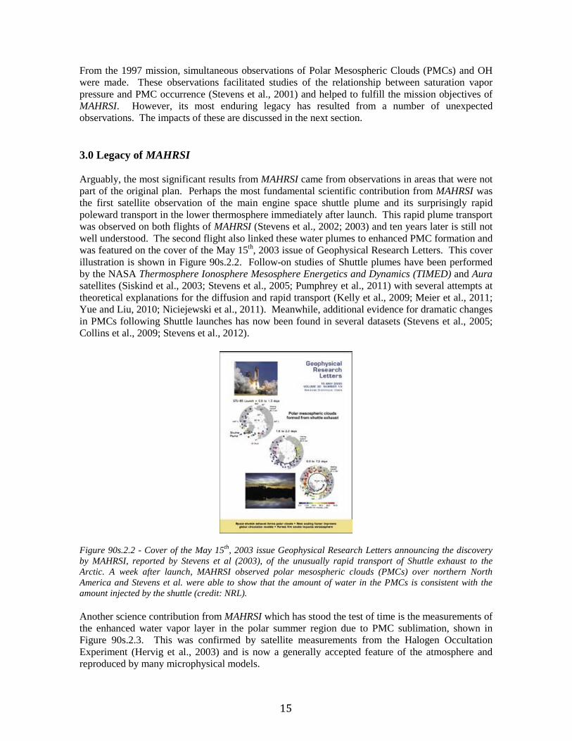
From the 1997 mission, simultaneous observations of Polar Mesospheric Clouds (PMCs) and OH were made. These observations facilitated studies of the relationship between saturation vapor pressure and PMC occurrence (Stevens et al., 2001) and helped to fulfill the mission objectives of MAHRSI. However, its most enduring legacy has resulted from a number of unexpected observations. The impacts of these are discussed in the next section. 3.0 Legacy of MAHRSI Arguably, the most significant results from MAHRSI came from observations in areas that were not part of the original plan. Perhaps the most fundamental scientific contribution from MAHRSI was the first satellite observation of the main engine space shuttle plume and its surprisingly rapid poleward transport in the lower thermosphere immediately after launch. This rapid plume transport was observed on both flights of MAHRSI (Stevens et al., 2002; 2003) and ten years later is still not well understood. The second flight also linked these water plumes to enhanced PMC formation and was featured on the cover of the May 15th, 2003 issue of Geophysical Research Letters. This cover illustration is shown in Figure 90s.2.2. Follow-on studies of Shuttle plumes have been performed by the NASA Thermosphere Ionosphere Mesosphere Energetics and Dynamics (TIMED) and Aura satellites (Siskind et al., 2003; Stevens et al., 2005; Pumphrey et al., 2011) with several attempts at theoretical explanations for the diffusion and rapid transport (Kelly et al., 2009; Meier et al., 2011; Yue and Liu, 2010; Niciejewski et al., 2011). Meanwhile, additional evidence for dramatic changes in PMCs following Shuttle launches has now been found in several datasets (Stevens et al., 2005; Collins et al., 2009; Stevens et al., 2012).

Figure 90s.2.2 - Cover of the May 15th, 2003 issue Geophysical Research Letters announcing the discovery by MAHRSI, reported by Stevens et al (2003), of the unusually rapid transport of Shuttle exhaust to the Arctic. A week after launch, MAHRSI observed polar mesospheric clouds (PMCs) over northern North America and Stevens et al. were able to show that the amount of water in the PMCs is consistent with the amount injected by the shuttle (credit: NRL). Another science contribution from MAHRSI which has stood the test of time is the measurements of the enhanced water vapor layer in the polar summer region due to PMC sublimation, shown in Figure 90s.2.3. This was confirmed by satellite measurements from the Halogen Occultation Experiment (Hervig et al., 2003) and is now a generally accepted feature of the atmosphere and reproduced by many microphysical models.

16

Figure 90s.2.3 - Observation of enhanced water vapor formed by sublimating PMCs. The shaded curve called “Inferred H2O” is obtained by conversion of MAHRSI OH measurements into H2O using photochemical theory. The predicted H2O from conventional theory is the curve called “2D model H2O” and the HALOE (Halogen Occultation Experiment, on the NASA/UARS satellite) H2O is observational confirmation of the MAHRSI results (from Summers et al., 2001)(credit: NRL). A third unexpected contribution from MAHRSI was the first ultraviolet (UV) detection of mesospheric water vapor (Stevens et al., 2008). When water vapor is photodissociated in the upper mesosphere, some of the OH that is produced is rotationally excited and the detection of these weaker “OH prompt” emissions is a direct measure of the water vapor concentrations. These OH prompt observations were obtained with special operations during the second mission that suppressed the Rayleigh scattered background and allowed for higher quality spectra from which the emission could be detected. Programmatically, MAHRSI formed the intellectual foundation for the NRL Spatial Heterodyne Imager for Mesospheric Radicals (SHIMMER) program that launched in 2007 and provided key theoretical support for the NASA Aeronomy of Ice in the Mesosphere (AIM) mission that launched in 2007. SHIMMER was a 30 month long mission to repeat the MAHRSI observations over diurnal, seasonal and interannual time scales and to do it with a radically new technology, Spatial Heterodyne Spectroscopy (SHS). Using SHS, SHIMMER was able to achieve the performance of MAHRSI but with a payload size and mass that was less than 1/5 that of MAHRSI thus enabling it to be flown on a small satellite rather than the space Shuttle payload bay. The SHIMMER effort is described by Englert (2012, this history (the 2000s chapter)). On the AIM mission (Russell et al., 2009), NRL has played an important role in understanding the data and extending the results first obtained by MAHRSI. References: 90s.2: Middle Atmosphere High Resolution Spectrograph Investigation (MAHRSI)

1. Collins, R.L. et al., Noctilucent cloud in the western Arctic in 2005: Simultaneous lidar and camera observations and analysis, J. Atm. Sol.-Terr. Phys., 71, 446-452, 2009.

2. Conway, R.R., M.H. Stevens, J.G. Cardon, S.E. Zasadil, C.M. Brown, J.S. Morrill, and G.H. Mount, Satellite Measurements of Hydroxyl in the Mesosphere, Geophys. Res. Lett., 23, 2093-2096, 1996.

3. Conway, R.R., M.H. Stevens, C.M. Brown, J.G. Cardon, S.E. Zasadil, and G.H. Mount, The Middle Atmosphere High Resolution Spectrograph Investigation, J. Geophys. Res., 104, 16327-16348, 1999.

4. Conway, R.R., M.E. Summers, M.H. Stevens, J.G. Cardon, P.Preusse, and D. Offermann, Satellite Observations of Upper Stratospheric and Mesospheric OH: The HOx Dilemma, Geophys. Res. Lett., 27 , D.E. Siskind et al., eds., 2613-2616, 2000.

17

5. Englert, C.R., M.H. Stevens, D.E. Siskind, J.M. Harlander and F.L. Roesler, The Spatial Heterodyne Imager for Mesospheric Radicals (SHIMMER) on STPSat-1, J. Geophys. Res., 115, D20306, doi:10.1029/2010JD014398, 2010.

6. Gattinger, R.L. et al., Optical Spectrograph and Infra-Red Imaging System (OSIRIS) observations of mesospheric OH A2Σ+--X2P 0-0 and 1-1 band resonance emissions, J. Geophys. Res., 111, D13303, doi:10.1029/2005JD006369, 2006.

7. Hervig, M. E., M. McMugh, and M. E. Summers, Water vapor enhancement in the polar summer mesosphere and its relationship to polar mesospheric clouds, Geophys. Res. Lett., 30, 2041, doi:10.1029/2003GL018089, 2003.

8. Kelley, M. C., C. E. Seyler, and M. F. Larsen,Two-dimensional turbulence, space shuttle plume transport in the thermosphere, and a possible relation to the Great Siberian Impact Event, Geophys. Res. Lett., 36,L14103, doi:10.1029/2009GL038362, 2009.

9. Meier, R.R. et al., A study of space shuttle plumes in the lower thermosphere, J. Geophys. Res., 116, A12322, doi:10.1029/2011JA016987, 2011.

10. Niciejewski, R. et al., Verification of large-scale rapid transport in the lower thermosphere: Tracking the exhaust plume of STS-107 from launch to the Antarctic, J. Geophys. Res., 116, A05302, doi:10.1029/2010JA016277, 2011.

11. Pumphrey, H.C. et al., Observation of the exhaust plume from the space shuttle main engines using the microwave limb sounder, Atmos. Meas. Tech., 4, 89-95, 2011.

12. Russell. J.M. III et al., The Aeronomy of Ice in the Mesosphere mission, J. Atm Solar Terr Phys.., 2009.

13. Siskind, D. E., M. H. Stevens, J. T. Emmert, D. P. Drob, A. J. Kochenash, J. M. Russell III, L. L. Gordley, and M. G. Mlynczak, Signatures of shuttle and rocket exhaust plumes in TIMED/SABER radiance data, Geophys. Res. Lett., 30, 1819, doi:10.1029/2003GL017627, 2003.

14. Stevens, M.H., Nitric Oxide γ Band Fluorescent Scattering and Self-Absorption in the Mesosphere and Lower Thermosphere, J. Geophys. Res., 100, 14,735-14,742, 1995.

15. Stevens, M.H., R.R. Conway, J.G. Cardon, and J.M. Russell, III, MAHRSI Observations of Nitric Oxide in the Mesosphere and Lower Thermosphere, Geophys. Res. Lett., 24, 3213-3216, 1997.

16. Stevens, M.H. and R.R. Conway, Calculated OH A2Σ+ - X2Π (0,0) Band Rotational Emission Rate Factors: Comparison with MAHRSI Observations, J. Geophys. Res., 104, 16369-16378, 1999.

17. Stevens, M.H., R.R. Conway, C.R. Englert, M.E. Summers, K.U. Grossmann and O.A. Gusev, PMCs and the Water Frost Point in the Arctic Summer Mesosphere, Geophys. Res. Lett., 28, 4449-4452, 2001.

18. Stevens, M.H., C.R. Englert, J. Gumbel, OH observations of space shuttle exhaust, Geophys. Res. Lett., 29(10), 10.1029/2002GL015079, 2002.

19. Stevens, M.H., J. Gumbel, C.R. Englert, K.U. Grossmann, M. Rapp and P. Hartogh, Polar mesospheric clouds formed from space shuttle exhaust, Geophys. Res. Lett., 30(10), 1546, doi: 10.1029/2003GL017249, 2003.

20. Stevens, M.H. et al., Antarctic mesospheric clouds formed from space shuttle exhaust, Geophys. Res. Lett., 32, L13810, doi:10.1029/2005GL023054, 2005.

21. Stevens, M.H., R.L. Gattinger, J. Gumbel, E.J. Llewellyn and D.A. Degenstein, First UV satellite observations of mesospheric water vapor, J. Geophys. Res., 113, D12304, doi: 10.1029/2007JD009513, 2008.

22. Stevens, M.H., S. Lossow, J. Fiedler, K. Hallgren, P. Hartogh, C.E. Randall, J. Lumpe, S.M. Bailey, R. Niciejewski, R.R. Meier, J.M.C. Plane, A.J. Kochenash, D.P. Murtagh and C.R. Englert, Bright polar mesospheric clouds formed by main engine exhaust from the space shuttle’s final launch, submitted to J. Geophys. Res., 2012.

23. Summers, M.E., R.R. Conway, C.R. Englert, D.E. Siskind, M.H. Stevens, J.M. Russell, III, L.L. Gordley, and M.J. McHugh, Discovery of a Layer of Water Vapor in the Arctic Summer Mesosphere: Implications for Polar Mesospheric Clouds, Geophys. Res. Lett., 28, 3601-3604, 2001.

24. Yue, J. and H.-L. Liu, Fast meridional transport in the lower thermosphere by planetary-scale waves, J. Atm. Sol.-Terr. Phys., 72, 1372-1378, 2010.

18

90’s.3I: ARGOS PART I: SSD Experiments on ARGOS – Overview

Contributed by Kent S. Wood, Michael Lovellette, and Kenneth Dymond 1.0 Introduction During the late 1990s the DoD Space Test Program (STP) undertook development of a major satellite to carry a suite of experiments selected by the Space Experiment Review Board (SERB). Originally manifested by STP as P91-1, it was eventually named the Advanced Research and Global Observation Satellite (ARGOS) and carried eight experiments, six proposed by NRL. Among those NRL payloads, five were provided wholly or in part by the Space Science Division (SSD). Three of the five, USA, GIMI, and HIRAAS, were led by the Space Science Division, and are described here. The other two, Extreme-ultraviolet Imaging Photometer (EUVIP) and Space Dust experiment (SPADUS), were primarily developed by university groups and the NRL role was collaborative and secondary. When the mission was well advanced in development a ninth payload was added from the Plasma Physics Division at NRL, Coherently Emitting Radio Tomography experiment (CERTO). This historical presentation is organized into four parts or chapters, one for each of the principal SSD experiments separately and a first chapter (this one) to cover ARGOS itself plus aspects of how the three SSD payloads were coordinated from the time of mission commitment to delivery. This was the job of the ARGOS Experiments Office created within SSD to guarantee delivering the three SSD experiments efficiently with simultaneous parallel development and modest staffing. A further story that emerges is that this process proved enabling to the overall effort in technical ways. The chapters describing ARGOS are:

I. SSD Experiments on ARGOS - Overview II. The USA Experiment

III. The High Resolution Airglow and Aurora Spectroscopy (HIRAAS) Experiment for the Advanced Research and Global Observation Satellite (ARGOS)

IV. The Global Imaging Monitor of the Ionosphere (GIMI) Experiment 2.0 ARGOS Mission and the ARGOS Experiments Office Basic characteristics of the ARGOS mission are summarized here, which avoids repeating them for each of the three experiments. The satellite bus contract was initially won by Rockwell International and initial technical interchanges and program development were done with their staff. Later acquisition of Rockwell by Boeing meant ARGOS was a Boeing spacecraft when launched. The 5000 lb (2350 kg) spacecraft was launched on a Delta-2 on Feb 23, 1999, after ten previous scrubbed launch attempts. Two Air Force experiments, Electric Propulsion Space Experiment (ESEX), an arcjet propulsion system, and a Critical Ionization Velocity experiment (CIV), were operated during the second phase of the mission, the first being space vehicle initialization. After the second phase was terminated by the explosion of the ESEX battery, the other experiments were turned on. These were environmental sensors arranged to be operationally non-interfering to permit taking data simultaneously. The spacecraft managed the commanding and data downlink for all experiments with several experiments sharing a MIL-STD 1553 bus for command and data transfer. The orbit was 830 km Sun-synchronous (98 deg. Inclination), partly to approximate the orbit in which sensors prototyped on ARGOS would later fly in operational applications, that is, an orbit like that of Defense Meteorological Satellite Program (DMSP) satellites. The website https://en.wikipedia.org/wiki/ARGOS_(satellite). provides an accessible summary of other aspects

19

of the mission: Delivering three quite different but ambitious experiments to the same launch posed a considerable challenge to the X-ray Astronomy Branch of SSD, which had primary responsibility for USA and HIRAAS and a supporting role in GIMI as well. The Experiments Office was set up for several purposes, including management and oversight, but was also charged with containing the cost of the experiments. Division Superintendent H. Gursky assigned the coordination responsibility to G. Fritz, Branch Head for X-ray Astronomy, Code 7620. The ARGOS Experiments Office was established at ARGOS mission definition, in 1991. NRL commitment became final in 1992. The Experiments Office lasted for a decade, during which time the experiments were designed, reviewed, built, tested, and flown. The office began to phase out as the experiments entered data analysis. The Experiments Office facilitated the development of common spacecraft interfaces and joint procurements for common components. While it was beneficial to try to exploit these commonalities the situation had not been anticipated in advance of the establishment of the ARGOS mission. Another programmatic feature was SERDP, the Strategic Environmental Research and Development Program, conducted jointly by the Department of Defense with Department of Energy, the Environmental Protection Agency, and other organizations. The premise of this program was that DoD was gathering extensive data by remote sensing of the Earth and useful for Earth system science. If not classified, such data could be made accessible to the broader research community and SERDP was intended to facilitate this. NRL received funding under SERDP to bring its ARGOS experiments within the compass of that concept. This funding helped make up part of the funding needed to build each experiment but it also funded the ARGOS Experiments Office. Meeting the SERDP program objective helped with building programmatic unity out of the selected SERB experiments and also with standardizing the data flow and enabling mission aspects conducive to good data quality. The payloads were all regarded as experiments, Class C in the terminology of MIL-HNBK-341, while the bus was Class B. This minimized the amount of documentation required, although the overall scale of ARGOS was large and drove it toward the characteristics of a major science mission. The bulk of the common interface documentation was handled by one person within the coordination office, L. Scoggin. The experiment specific aspects were handled by the individual teams, and there was constant interfacing with the mission integration team provided by STP and the Rockwell/Boeing contractor team. Flying a diverse suite of experiments necessitated many technical interchange meetings to resolve potential conflicts in areas such as fields of view, interfaces, or operating constraints. The Experiments Office assisted NRL experimenters in coordinating these matters with STP in a way that left each of the three SSD experiments considerable autonomy. Initially ARGOS was rather limited in respects such as orbital knowledge, aspect information, commanding for optimization of operations and implementation of data flow, but the approach of seeking to exploit commonalities not only for economy but for enhancement as well brought significant benefits the time of launch. It became the first satellite to use GPS for onboard orbital reference and it developed streamlined commanding procedures. This experience was passed on not only to DoD but to NASA. Experience with onboard processing for ARGOS carried forward into NRL’s later involvement with NASA’s Fermi mission. (See USA Essay 90s.3II, following.) Overall, solutions to space computing problems used on ARGOS were advanced for their day but by now have been superseded by later and often simpler methodologies.

20

3.0 Design Coordination to Meet ARGOS Specifications; the Gimbal Issue ARGOS underwent a rather complex initial sorting out of the requirements of its principal experiments culminating in a System Requirements Review (SRR). Demands on power, commanding, and telemetry were reconciled, as were viewing and other operational conflicts. Details such as the need for a GPS receiver onboard to provide spacecraft time and position determination were worked. Extensive technical interchanges were carried out before and after SRR to resolve these issues. The mission architecture was refined in the System Design Review (SDR), the Preliminary Design Review (PDR), and the Comprehensive Design Review (CDR) until a considerable degree of unification was achieved out of the initial heterogeneity. Three specific design issues illustrate this. First, the use of the MIL-STD 1553 bus meant that most instruments needed the same bus interface, and this became a common design feature. Second, ARGOS was offered to experimenters as a nadir-pointed spacecraft and it was necessary for USA, HIRAAS, and GIMI to do offset pointings whether for astronomy or for scanning limb observations. Had there not been the three gimbals the several experiments would have had to take turns being prime and the pointing task would have been levied on the spacecraft. Thus finding a triple-gimbal solution was enabling for the functionality of all experiments. Commonality was exploited wherever possible, common design elements such as stepper motors and pointing processor boards were used, and common vendors for other components such as shaft angle encoders. Finally, the encoder, motor and processor solutions for the gimbals were also adapted for use internal to the HIRAAS experiment to operate the grating drive mechanism in the High-resolution Ionosphere and Thermosphere Spectrograph (HITS) instrument. 4.0 Coordination of Procurements

The Experiments Office coordinated procurements as well as documentation, organizing nearly-daily group meetings to define parts needs, carry out competitive evaluations, and undertake bulk purchases. There were benefits and risks. A bad procurement would risk saddling three experiments rather than one with a problematic component. Mention has already been made of how the Harris 80C86 rad-hard processor became used in all experiments for central processing and for pointing control. This decision led into subsequent commonalities in interfacing and software development. All of the 80C86’s used a common boot code. Two programmers shared tasks on multiple experiments. The Harris 80C86 processors, shaft angle encoders and stepper motors were all examples of bulk buys. The three experiments could also pool experience with components that had originated in bulk purchases. 5.0 Construction Phase, Problem Resolution, Testing The Integration and Test phase was centered at NRL. Both USA and HIRAAS had outside university partners but even when those partners produced major subsystems NRL undertook top level integration. Test of the completed experiments was done at NRL using facilities of the Naval Center for Space Technology (NRL Code 8000), with Experiment Office oversight and coordination with STP. The handling of commanding and data both on the ground and in space illustrated the benefits of coordination. The Laboratory for Astrophysical and Solar Plasmas (LASP) at Boulder CO undertook development of software systems used in Ground Support Equipment (GSE) and in space. Experiment teams tailored this software to their needs. After experiment delivery to Boeing there was a lengthy integration and test period at the contractor as vehicle issues were diagnosed and corrected. T. Crandall of the Space Science Division (NRL/SSD) worked with the USA team and under the Experiment Office to develop noteworthy capabilities. A software socket interface he invented incorporated a web interface that permitted data transfer across the World Wide Web even when the experiment was not at NRL. During the thermal/vacuum test at the spacecraft vendor (which by then was Boeing) it was possible for USA

21

experimenters to sit at NRL and view experiment data screens as though they were present at the facility in California. During space vehicle integration and test and launch site operations M. Lovellette of NRL/SSD served as the principal spokesman for the three SSD experiments and occasionally EUVIP and SPADUS. Test as You Fly methodologies were developed with STP and used to verify complex Phase 3 space vehicle operations timelines. Testing was rendered more complex than usual because each of the Phase 3 experiments operated independently and simultaneously which placed continually varying loads on the space vehicle power and telemetry subsystems. The figures illustrate the end result. Figure 90s.3I.1 is the ARGOS satellite when being stacked up onto the launch vehicle. It is easy to recognize NRL’s USA Experiment as the uppermost part of the payload in the launch configuration. Figure 90s.3I.2 shows the completed vehicle on the pad at VAFB awaiting launch.

Figure 90s.3I.1 - ARGOS spacecraft in preparation for launch at Vandenberg AFB. The USA experiment, which is on the aft end of the spacecraft when launched, is visible at the top of the stack (credit: NRL).

Figure 90s.3I.2 - ARGOS on the launch pad on the evening of the first launch attempt (credit: NRL).

22

6.0 Summary The ARGOS Experiments Office was a practical solution to the logistics challenge presented by simultaneous delivery of the SSD payloads. Payloads were mostly built and integrated in-house but with extensive procurement of components and subsystems from outside vendors and suppliers. Some features of how the SSD experiments were executed derive from this coordination approach. This chapter most likely provides the only narrative history extant of how it was accomplished.

Table of ARGOS Mission Characteristics

Management: DoD Space Test Program

The 5000 Ib. ARGOS satellite was launched by a Delta II launch vehicle from Vandenberg AFB at 1030 UT (0230 local time) on 23 February 1999. The spacecraft was operated in a 3-axis stabilized mode with the Z-axis always pointed to nadir. Attitude control is based on a system of gyros and horizon sensors feeding into reaction wheels and C02 thrusters. The orbit was nearly circular with ~830 km altitude and 98.7 degree inclination. It was Sun synchronous with a beta angle of 25-45 degrees. (The nadir scanned along Earth surface regions at roughly 2 am and 2 pm local time.) Spacecraft Boeing, Seal Beach CA (originally Rockwell International)

LV Delta II Launch VAFB, Feb 23, 1999 Mass 2350 kg Orbit 833 km Sun synchronous Data rates 4 and 128 kbps

Experiments NRL:

USA X-ray sensor, computer test bed HIRAAS Spectrometers for thermosphere/ionosphere studies GIMI Telescopes for ionospheric imaging EUVIP EUV sensor (UC Berkeley PI; NRL assistance) SPADUS Space dust experiment (U of Chicago PI, NRL assistance) CERTO Radio beacon for ionosphere studies. HTSSE High temperature superconducting components tests

AFRL: ESEX Arcjet thruster CIV Critical ionization velocity experiment

References: 90s.3I: ARGOS PART I: SSD Experiments on ARGOS - Overview

1. “Testing Issues During the USAF Space Test Program’s ARGOS Satellite Development,” Lovellette, M. N., Chism, D. D., La Grassa, M., Quintero, A., and White, J. D., in Proceedings of 19th Aerospace Testing Seminar, held in Manhattan Beach CA, 2 October – 5 October 2000, The Aerospace Corporation, (2000).

23

90’s.3II: ARGOS PART II: The USA Experiment

Contributed by Kent S. Wood and Michael Lovellette

1.0 Introduction The Unconventional Stellar Aspect (USA) was an X-ray astronomy experiment carried out under STP, with applied aspects that were not astronomical. The P.I. was K. Wood, then in the X-ray Astronomy Branch, SSD (Code 7620). That Branch took primary responsibility for building USA. The secondary aspect of computing in space became important as a subsystem with its own line of sponsorship and research objectives, hence was sometimes referred to separately as ASCAT, for Advanced Space Computing and Autonomy Testbed. ASCAT was led by M. Lovellette of NRL/SSD. This section describes the program, instrument, and flight results, with historical perspectives. USA had four quite distinct objectives, not a single research focus. The original scientific interest centered on celestial X-ray sources but the uniqueness of the experiment was pioneering three allied areas, each applied in nature and each remaining active today: X-ray navigation, X-ray aeronomy, and the first testbed for comparative space-based computing. They are characterized as “allied” because they derived from use of X-ray sensors in space; two depended on sensing celestial sources. The experiment system was two proportional counters mounted in a two-axis gimbal for offset pointing from nadir-pointed ARGOS, plus the computer testbed (ASCAT) residing inside the central electronics box. Programmatic Background for USA at NRL USA was developed under NRL’s X-ray astronomy program, but its flight redefined program directions. Earlier highlights (sounding rockets, High Energy Astrophysical Observatories HEAO-1) have been covered in other chapters of this SSD history. NRL’s investment in X-ray astronomy had begun with work of H. Friedman and colleagues, mapping celestial X-ray sources in the sky and understanding their intrinsic characteristics so as to deal with them as backgrounds to any sensor systems DoD might operate. That formulation was not specific as to the potential X-ray applications. Cataloging became complex because the X-ray sky exhibits tremendous diversity among its bright features. The diversity revealed itself gradually, extending characterization of source populations to an international project spanning decades. By the 1980s surveys such as Uhuru and HEAO-1 had established X-ray point sources were variable, almost without exception. There were also extended sources constant over long times. When USA was conceived, cataloging fainter sources levels had become the goal of the German satellite Rosat, then in preparation. 2.0 Research Program: Four Research Thrusts Within the evolving NRL X-ray program there was growing interest in using source observations to pursue topics in fundamental physics associated with extreme physical conditions in what were still rather recently-discovered classes of objects, primarily neutron stars and black holes. The physics of strong gravity, dense matter, and strong magnetic fields was more approachable astrophysically than in the laboratory. This motivation was shared by two groups at Stanford University, in the Physics Department and at Stanford Linear Accelerator Center (SLAC). It remains viable today and still only partly realized. One dream dating from the 1980s still remains years from realization today, although variants on it are under active consideration. This was the X-ray Large Array (XLA). Initial study of XLA led to USA. XLA sought to attack basic physics questions using many square meters of X-ray aperture to harvest X-rays at very high rates (millions per second),

24

permitting exploration of variability at millisecond to microsecond timescales. XLA had strong backing from H. Friedman and H. Gursky at NRL and from W. Fairbank and R. Hofstadter at Stanford. Hofstadter in particular urged pursuit of the largest feasible collecting aperture, nominally 100 m2, which entailed placing XLA on the International Space Station (ISS). (See Wood et al., 2004 for further detail on XLA.) It became clear from a NASA Phase A study that XLA on the ISS would be a major undertaking needing broad community support, more than it actually enjoyed. Surveying and quantifying potential scientific uses for such large area had produced two distinct lists of candidates. Goals on the first list absolutely required many square meters of aperture and were otherwise unattainable. The second list consisted of goals that could be accomplished with a lesser aperture by adopting the tactic of accumulating large observing time suitable sources, usually brightest members of their classes. That list became USA, a timing experiment with a “niche” of large exposure (= area x time product), achieved with a modest aperture. Hardware for that science also supported applied topics, X-ray navigation and aeronomy. A group at the Naval Postgraduate School (NPS) was then promoting a small satellite bus for STP. Discussions with NPS led to the earliest concept for USA. Within a year USA outgrew the NPS bus concept and emerged as a more ambitious payload that could attach to a major satellite, because the idea of ARGOS was gaining support. If USA were placed on a nadir-pointed satellite, mounting at the aft end would be protective of its thin windows (see this Chapter Sec. 3.0), which in turn implied sources would move downward to the horizon while being tracked and monitored. Watching X-ray sources set into the atmosphere was an X-ray realization of the horizon-crossing technique well-known to satellite navigation, but also led directly to a tool for aeronomy because the occultation curve depended on atmospheric density. Navigation created a desire to have good onboard computing. (See this Chapter Sec. 2.4.) When the time came to select a name for the STP payload H. Gursky argued it should emphasize the applications and he proposed “unconventional stellar aspect.” The acronym had obvious advantages hence the name stuck. As hope of XLA faded while USA moved toward realization, the applied side of the enterprise grew in prominence. The four research thrusts of USA are now treated individually in further detail. 2.1 X-ray timing astrophysics The brightest variable X-ray sources are, with some exceptions, powered by accretion onto neutron stars or black holes such that the X-ray luminosity is the gravitational potential multiplied by the mass accretion rate. Complex fluid flows occurring in these sources (often binary stellar systems) produce surprisingly varied phenomenology, i.e., “weather,” but on prodigious scales of energy release and violence. There are other effects such as regular pulsations (from rotation of magnetized stars) and eclipses, in the binaries. Some of these signatures had potential for providing timekeeping. The metaphor of a natural GPS system became commonplace. These aspects of USA (X-ray phenomenology and timekeeping applications) were essential to secure the STP flight. They also drove instrument requirements. Orbital timescales near neutron stars and black holes are in the millisecond range. Short timescale measurements could probe physical processes in extreme regimes by reaching their dynamical timescales. The Crab Nebula is a useful reference for source brightness and produces a flux at Earth of about 10 photons cm-2 s-1 in 1-10 keV X-rays. A "milliCrab" is a flux 0.001 that of the Crab Nebula. For sources brighter than a few milliCrabs, detectors of the USA size could be effective. 2.2 X-ray Navigation This topic meant X-ray determination of attitude, position, or local time by an X-ray sensor on a satellite platform. USA was the first testbed for this idea. Prelaunch papers (Wood., 1993; Wood et al., 1994) that developed the rationale for USA also laid out the broad outlines for X-ray navigation. Another goal of interest was time transfer between two satellites by having them

25

observe the same celestial source. Use of pulsars was one way to do position determination or timekeeping. Because of acceleration in orbits near planets another technique was observations of occultations, transitions where the line of sight to a source crosses the horizon. On an airless planet it would be the hard rock horizon but for low Earth orbit the horizon would be defined by the tangent line of sight where the atmosphere absorbed X-rays. Measuring in-track position in LEO by these occultations calls for knowledge of atmospheric density and composition. The atmospheric model dictates the precise shape of the occultation curve. If the model is accurate, the occultation time gives the satellite position at the transition time. Multiple occultations yield orbital elements. 2.3 X-ray aeronomy In a different utilization, the data for an X-ray occultation curve may be used to measure the atmospheric density profile (at occultation time and near the tangent point), treating the orbit solution as an input rather than as the deliverable. USA was designed to explore both goals. The USA sensor gave density diagnostics at roughly 80-160 km. The altitude probed goes inversely with photon energy; extreme ultraviolet (EUV) sensors could use the method at higher altitudes. For altitudes covered by USA there was growing awareness from the work of R. Roble that greenhouse gas buildup could in principle modify density and temperature profiles. Global warming at sea level becomes global cooling above the thermopause, at 90 km (Roble and Dickinson, 1989; Roble, 1995). This aspect of USA related to the Strategic Environmental Research and Development Program (SERDP) described in the previous chapter, one of the unifying themes of ARGOS. 2.4 Reliable Computing in Space X-ray navigation created need for onboard computing. If the idea is to use the X-ray sensor for satellite navigation it is artificial or even pointless to obtain the navigational solution (state vector) on the ground months afterward; far better to generate it onboard in real time. At the time when USA was being conceptualized the closing of rad-hard foundries combined with accumulating experience regarding processor malfunctions in space was producing a favorable climate for research on space-based computing. The period from establishment of the ARGOS mission to launch was a time in which this aspect of the experiment was continually upgraded. To capture the flavor of those times, one must know rad-hard processors used in space were 16 bit machines of limited throughput. There were parallel efforts ongoing to advance the state of the art to rad-hard 32-bit processors. R. Bleach and L. Lome as well as A. Fox in NRL Code 8000 helped establish this part of USA. A “processor showcase” event helped define rad-hard 32-bit options. The USA team sought to fly as many processors as possible in a mode that would compare performance and the USA electronics box was designed to hold and operate four of them. However at a certain point it became clear only the Harris RH3000 provided by NRL Code 8000 would be delivered in working order in time for launch. There was at the time widespread interest in the possibility that commercial off-the-shelf (COTS) processors might be made serviceable, particularly ones demonstrated to be somewhat rad-tolerant. Along with this went the idea that fault tolerance software might upgrade the performance of a COTS processor and make it competitive. This became the goal of the USA processor testbed, ASCAT. Prof. E. McCluskey of Stanford and his students joined in the effort, which was already sponsored by the Strategic Defense Initiative Organization (SDIO), and together the experiment was reconfigured around comparison of the rad hard processor with the COTS one (IDT 3081), with both having the benefit of the fault tolerant software. Evolution of the processor testbed is further described in Lovellette et al., 2002, 2003 and Shirvani et al., 2001 and in two Ph.D. theses in Electrical Engineering done at Stanford.

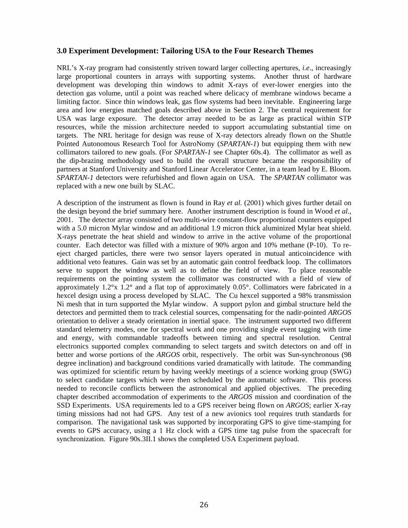
26

3.0 Experiment Development: Tailoring USA to the Four Research Themes NRL’s X-ray program had consistently striven toward larger collecting apertures, i.e., increasingly large proportional counters in arrays with supporting systems. Another thrust of hardware development was developing thin windows to admit X-rays of ever-lower energies into the detection gas volume, until a point was reached where delicacy of membrane windows became a limiting factor. Since thin windows leak, gas flow systems had been inevitable. Engineering large area and low energies matched goals described above in Section 2. The central requirement for USA was large exposure. The detector array needed to be as large as practical within STP resources, while the mission architecture needed to support accumulating substantial time on targets. The NRL heritage for design was reuse of X-ray detectors already flown on the Shuttle Pointed Autonomous Research Tool for AstroNomy (SPARTAN-1) but equipping them with new collimators tailored to new goals. (For SPARTAN-1 see Chapter 60s.4). The collimator as well as the dip-brazing methodology used to build the overall structure became the responsibility of partners at Stanford University and Stanford Linear Accelerator Center, in a team lead by E. Bloom. SPARTAN-1 detectors were refurbished and flown again on USA. The SPARTAN collimator was replaced with a new one built by SLAC. A description of the instrument as flown is found in Ray et al. (2001) which gives further detail on the design beyond the brief summary here. Another instrument description is found in Wood et al., 2001. The detector array consisted of two multi-wire constant-flow proportional counters equipped with a 5.0 micron Mylar window and an additional 1.9 micron thick aluminized Mylar heat shield. X-rays penetrate the heat shield and window to arrive in the active volume of the proportional counter. Each detector was filled with a mixture of 90% argon and 10% methane (P-10). To re-eject charged particles, there were two sensor layers operated in mutual anticoincidence with additional veto features. Gain was set by an automatic gain control feedback loop. The collimators serve to support the window as well as to define the field of view. To place reasonable requirements on the pointing system the collimator was constructed with a field of view of approximately 1.2°x 1.2° and a flat top of approximately 0.05°. Collimators were fabricated in a hexcel design using a process developed by SLAC. The Cu hexcel supported a 98% transmission Ni mesh that in turn supported the Mylar window. A support pylon and gimbal structure held the detectors and permitted them to track celestial sources, compensating for the nadir-pointed ARGOS orientation to deliver a steady orientation in inertial space. The instrument supported two different standard telemetry modes, one for spectral work and one providing single event tagging with time and energy, with commandable tradeoffs between timing and spectral resolution. Central electronics supported complex commanding to select targets and switch detectors on and off in better and worse portions of the ARGOS orbit, respectively. The orbit was Sun-synchronous (98 degree inclination) and background conditions varied dramatically with latitude. The commanding was optimized for scientific return by having weekly meetings of a science working group (SWG) to select candidate targets which were then scheduled by the automatic software. This process needed to reconcile conflicts between the astronomical and applied objectives. The preceding chapter described accommodation of experiments to the ARGOS mission and coordination of the SSD Experiments. USA requirements led to a GPS receiver being flown on ARGOS; earlier X-ray timing missions had not had GPS. Any test of a new avionics tool requires truth standards for comparison. The navigational task was supported by incorporating GPS to give time-stamping for events to GPS accuracy, using a 1 Hz clock with a GPS time tag pulse from the spacecraft for synchronization. Figure 90s.3II.1 shows the completed USA Experiment payload.

27

Figure 90s.3II.1 - The USA experiment mounted in its pointing mechanism. The figure shows an oblique view of the front of the detector. The four panels at the center of the aperture are the entry windows covered with their aluminized Mylar heat shields. Surrounding the detector the inner and outer gimbals and the supporting pylon can be seen (credit: NRL). 4.0 ARGOS Flight and Results The X-ray detectors were activated 29 April 1999 and operated until 16 November 2000, at which time both detectors had lost all their P-10 gas and could no longer function. The computing testbed continued to operate through August 2001. The USA program meant the USA team was active in four different research communities in deriving and publishing results during the flight years and immediately afterward. Thesis research was conducted in all four areas by graduate students from Stanford (engineering as well as physics), Maryland, and George Mason University. Results are now described, according to the thematic areas already introduced above. 4.1 X-ray Astrophysics Compact stellar objects such as white dwarfs, neutron stars, and black holes are the final states of stars whose nuclear fuel has been exhausted so that remaining support against gravity comes not from gas and radiation pressure but from Fermi pressure of electrons or hadrons. In a black hole, gravity has become too strong to permit even these configurations and the star has collapsed. All three types occur in nature, either in or outside of binary systems. Neutron stars have radii of ~10 km and typical masses of ~1.4 solar masses. Being in a binary system greatly enhances the visibility of any of these compact objects because gas transferred from the companion star falls into the deep gravitational potential well of the compact object and is heated until the source develops outstanding luminosity in X-rays. The great majority of the observations made with USA had either neutron star or black hole sources as targets. Target sources were either ones already catalogued or new transients appearing in the sky as the mission progressed. Nearly 10 megaseconds of data were gathered with the X-ray detectors pointed at various celestial targets. About 60 targets were observed overall but some were only surveyed briefly so that much time was concentrated on a smaller list. Included were accreting white dwarfs, neutron star pulsars (some in binary systems and some isolated), accreting neutron stars that are not pulsars, black hole candidates, and active galactic nuclei sources.

28

Transient black hole sources are one class where the USA observing strategy was used effectively. Four prominent transients active during the life of USA were XTE 111 18+480, XTE Jl550-564, XTE Jl859+226 and GRS 1915+105. It was possible to observe them many times a day for many consecutive days. The transient XTE J1118+480 in Ursa Major had an unusual double-outburst starting in January 2000. It was not initially noticed by monitors and it was only when the second outburst began that discovery was announced. The earlier outburst was then reconstructed from archival data. The earlier outburst was smaller and lasted -30 days while the second and brighter outburst lasted considerably longer. USA began extensive observations following the discovery. It was observed frequently for over 100 days until the source had faded. An orbital period of 4.1 hours was detected in concurrent optical observations and study of this orbit eventually led to the determination that the source was unusually massive and could not be a neutron star.

Both neutron star and black hole sources frequently exhibit quasi-periodic oscillations (QPOs). These oscillations are detected by taking Fourier transforms of many short segments of data and summing the results. The QPO shows as excess power at a particular frequency. A low-frequency QPO that was highly persistent was observed by USA during the second outburst of XTE Jl 118+480. This QPO drifted steadily upward in frequency during the time interval in which the overall source brightness reached maximum and began to decline (Wood et al., 2000). The observations of this QPO made with USA are the most complete data set available and show in detail how the QPO centroid frequency drifted. The USA team subsequently developed a model for evolution of the outburst in terms of deposition of matter at the outer edge of an accretion disk around the black hole and subsequent diffusion-driven evolution of the disk driving the matter into the black hole (Wood et al., 2000). Other black hole candidates observed by USA provided thesis material for students working with the group at SLAC led by E. Bloom that had helped build USA, including seven who completed Ph.D work in connection with USA: J. Hanson, H. Wen, G. Shabad, K. Reilly, P. Saz-Parkinson, D. Tournear, and D. Engovatov. (See also Reilly et al., 2002) (Two more Ph.Ds from Stanford and one from Maryland are mentioned elsewhere in this chapter, for a total of ten.)

Figure 90s.3II.2 (left) - Example of astrophysical use of USA. Complete outburst light curve of XTE J1118+480. The time axis is labeled as days since 1999 December 23. Diamonds are data from the RXTE/ASM and crosses are from USA. The greater sensitivity of USA is reflected in reduced scatter after day 110 where the USA data begin. The data have been interpolated and regridded so as to give one data point per day. The days covered are those on which the QPO in the next figure was observed (credit: NRL).

Figure 90s.3II.3 (right) - Comparison of the quasi-periodic oscillation (QPO) frequency evolution with the derived mass of the disk. The points are the QPO frequency according to the left axis (crosses are X-ray determined QPO frequencies from Wood et al. (2000) and diamonds are optically determined QPO frequencies from Haswell et al. (2000) and J Patterson & D. Skillman 2000, private communication). The dotted lines line pertain to models for varying mass in the accretion disk derived from the light curve and the solid line is the inverse of the estimated disk mass (credit: NRL).

29

An interesting example of an eclipsing source is the neutron star binary Exo 0748-676. The orbital period of this system is 3.82 hours and the eclipses that occur each orbit last for 492 seconds. At one time it had been considered that this might be a sufficiently precise clock to be useful for X-ray navigation but eclipse timings by satellite experiments including USA revealed significant erratic drifts in the orbital period and also some variations in the eclipse durations. This mysterious variability was the subject of a number of presentations and papers in the ARGOS era. (See Figure 90s.3II.4 and Wolff et al., 2002.) NRL researchers continued to study it with Rossi X-ray Timing Explorer (RXTE) after the end of ARGOS and were eventually able to attribute some of the variability to effects of activity in the normal star that is the non-compact member of this binary system (Wolff et al., 2002). Study of this source continues to the present time. In recent years the accretion has turned off and it has declined to very low flux levels. The USA data are part of the permanent archive of its years of high activity.

Figure 90s.3II.4 - Mid-eclipse timing residuals for observed eclipses of EXO 0748-676 during 1985-2000, from both the present study and those available in the literature. The residuals of the observed mid-eclipse time from the same constant-period model as in the figure, is plotted as a function of the barycenter-corrected observation date. The curved solid line is the constant-period derivative solution. The dotted line is a broken constant-period solution. No simple linear or quadratic ephemeris fits all the data points (credit: NRL).

4.2 X-ray Navigation

The first Ph.D. thesis on the topic of X-ray navigation was produced by J. Hanson, who worked on the hardware development while carrying out this study (Hanson, 1996). This and work cited earlier (Wood, 1993; Wood et al., 1994) show how USA contributed to development of X-ray navigation when still in the pre-launch phase.

Following launch, X-ray sources used for navigation exercises were variable point sources whose positions were known to better than an arc second and in some cases having useful temporal signature. To test determinations of attitude, position and time the sensor could be used variously as (i) an X-ray aspect sensor, (ii) an X-ray horizon sensor, and (iii) as a device for timing the periodic signals from the celestial sources to measure phase delays and convert them to position information. In the horizon-sensing mode the precise time of the horizon crossing is combined with an atmospheric model to determine position.

One of the first uses was an unplanned exercise in attitude determination that became necessary because the ARGOS pointing system was not functioning properly. Since USA was not an imaging system, attitude determination was done using transits of sources through the response of the collimator. If an X-ray source drifts slowly through the field of view (for example if inertial pointing is turned off and the instrument scans at the satellite’s rate) then it traces out the point response function which is roughly triangular. Early in the ARGOS mission, the USA team began

30

doing a maneuver called a “drift raster”" in which the instrument was repeatedly pointed near a known source and was then allowed to drift through it. From the times of maximum response on several sets of observations it was possible to derive values for four misalignment angles characterizing the combination of the spacecraft attitude control system and the USA instrument gimbals. An example of such a fit is shown in Figure 90s.3II.5. To obtain a useful fit it was necessary to combine observations of several sources so that the source elevation above the horizon was not always the same. Formal errors in fits were typically a few hundredths of a degree. While it was planned as a refinement to instrument calibration, it became essential to basic attitude determination on 18 August, 1999, when a software upload to the spacecraft resulted in loss of ability to acquire sources. The cause was not immediately recognized. Using the drift raster mode, USA was able to fit unknown errors in spacecraft roll and yaw and show that source acquisition could be recovered approximately by introducing suitable compensation into the USA pointing system. Eventually values in a faulty spacecraft attitude control table were updated, restoring nominal operations. This constituted demonstration of X-ray attitude determination directly supporting ARGOS operations. The incident was presented at meetings in the aerospace community, yielding the first publications on X-ray navigation providing feedback to satellite operations (Wood et al., 2001). Of course, the feedback was via ground analysis and not onboard computing.

Figure 90s.3II.5 - X-ray Attitude Determination. Fits of residuals in the positions of peak responses to a misaligned model. From these fits it could be shown that the ARGOS spacecraft was not pointing as intended. The results were used in trouble-shooting and correcting the problem (credit: NRL).

Timekeeping experiments depend on using the best astronomical clocks, isolated pulsars. The pulsar in the Crab Nebula is the brightest in the X-ray sky but it is not the most stable clock. The quality of timekeeping provided by a pulsar depends on intrinsic noise process affecting its spin period and other pulsars are more stable than the Crab. Nevertheless, its strong signal makes it the place where USA begins its timekeeping studies. Timing of the Crab Pulsar using the onboard GPS timing of ARGOS is found to agree with the predicted pulse position from radio measurements (Figure 90s.3II.6; Wood et al., 2001). The two agree to about 100 microseconds, approximately the accuracy of the radio ephemeris. The Crab Pulsar period for this epoch was 33.4033474094 milliseconds. The ultimate accuracy to which studies of this kind can be pursued with ARGOS is about 2 microseconds. Work is ongoing and this goal has not yet been reached. The ultimate limits of X-ray methods come from more stable pulsars such as PSR 1937+219, whose pulse period is 1.555780646881979 ms. It is among the most precise astronomical clocks known and is detected as an X-ray source.

31

Figure 90s.3II.6 - X-ray Timekeeping.(left)The Crab pulse profile seen with USA (2 cycles).(right) Comparison of the main pulse profile with the predicted centroid position form the radio ephemeris (credit: NRL). In the later data analysis phase extending after mission termination a second X-ray navigation Ph. D. thesis by S. Sheikh was done on pulsar techniques (2005). Concurrently, the NRL group with an engineering group at University of Maryland applied for and received a patent on the pulsar-related navigational methods. During the USA years this approach had grown more feasible because of the discovery of X-ray millisecond pulsars. NRL efforts in this area continue to the present time (see this Chapter Sec. 5.0). 4.3 X-ray Techniques for Aeronomy Horizon crossing measurements, which in principle provide in-track position determination (this Chapter Sec. 2.2) can also be used to measure atmospheric density (this Chapter Sec. 2.3), which was in fact their primary utilization in connection with USA. The time and position for the spacecraft were redundantly known from the ARGOS orbital information including the GPS system, and were used to derive column density in the atmosphere along various lines of sight. The information is derived redundantly using different energies and can be inverted to obtain atmospheric scale height. This became the research topic of a graduate student from George Mason University (J. Determan), retired from the USAF following service during the First Gulf War. USA observations were supplemented by additional observations made with RXTE. The principal source used was the Crab Nebula, which is reasonably stable on long timescales although it contains a pulsar and has in subsequent years come to be recognized as somewhat variable. This work led to a paper that developed the occultation technique for atmospheric density fully for the first time (see Determan et al., 2007). 4.4 Reliable Computing in Space – the ASCAT Testbed The heart of the computing testbed, ASCAT, was a pair of computer boards, one rad-hard and the other COTS. The rad-hard board, the RH3000, was built around a pair of radiation-hardened Harris Semiconductor processors similar to the MIPS R3000, configured as a shadow pair with 2MB of memory. The IDT3081 board incorporated the commercial-off-the-shelf IDT3081 processor and 2 MB of Dynamic Random Access Memory (DRAM) without any special error correction hardware. Both computer boards had access to the downlink science telemetry stream. These processors have been operated with test software of various kinds, some of it with fault tolerance features. The processors were not required for the operation of the X-ray experiment but they could accept data from it. They were used for comparative experiments in fault tolerance. The radiation hardening development had required enough time that the rad-hard board had less processing power, compared to the COTS one. The ARGOS orbit, which was selected to be close to that of the

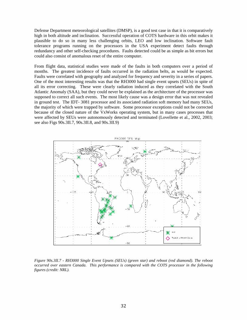
32

Defense Department meteorological satellites (DMSP), is a good test case in that it is comparatively high in both altitude and inclination. Successful operation of COTS hardware in this orbit makes it plausible to do so in many less challenging orbits, LEO and low inclination. Software fault tolerance programs running on the processors in the USA experiment detect faults through redundancy and other self-checking procedures. Faults detected could be as simple as bit errors but could also consist of anomalous reset of the entire computer. From flight data, statistical studies were made of the faults in both computers over a period of months. The greatest incidence of faults occurred in the radiation belts, as would be expected. Faults were correlated with geography and analyzed for frequency and severity in a series of papers. One of the most interesting results was that the RH3000 had single event upsets (SEUs) in spite of all its error correcting. These were clearly radiation induced as they correlated with the South Atlantic Anomaly (SAA), but they could never be explained as the architecture of the processor was supposed to correct all such events. The most likely cause was a design error that was not revealed in ground test. The IDT- 3081 processor and its associated radiation soft memory had many SEUs, the majority of which were trapped by software. Some processor exceptions could not be corrected because of the closed nature of the VxWorks operating system, but in many cases processes that were affected by SEUs were autonomously detected and terminated (Lovellette et al., 2002, 2003; see also Figs 90s.3II.7, 90s.3II.8, and 90s.3II.9)

Figure 90s.3II.7 - RH3000 Single Event Upsets (SEUs) (green star) and reboot (red diamond). The reboot occurred over eastern Canada. This performance is compared with the COTS processor in the following figures (credit: NRL).

33

Figure 90s.3II.8 - Summary of all IDT-3081 Single Event Upsets. Most of these events were not detrimental to performance because they were flagged and rejected by fault tolerance software (credit: NRL).

Figure 90s.3II.9 - Summary of all IDT-3081 task exceptions (blue crosses), critical exception reboots (green diamonds), and unknown reboots (red diamonds). This represents the performance of the COTS processor after correction by fault tolerance software. The residual rate of errors is not enormously greater than the rate in the rad-hard processor shown in Figure 90s.3II.7 (credit: NRL). 5.0 Aftermath and Legacy As ARGOS concluded the USA team and its Stanford colleagues were beginning to study a γ-ray mission based on silicon strip detectors, the one that became the Gamma Ray Large Area Space Telescope (GLAST) in development and Fermi after launch. Most of the USA team at NRL and Stanford went on to work on Fermi. Solid state detectors for X-rays as well as γ-rays began to be seen as preferable to proportional counters. The NRL X-ray group developed new solid state flight concepts. NRL proposed a follow-on to USA called SIXI (Silicon X-ray Imager) that never flew but a similar concept was flown as the Italian payload AGILE. USA experience with onboard computing led into an NRL role in development of onboard data acquisition and flight software for Fermi. The scientific and applied results made similar transitions. NRL continues to pursue compact object variability and navigation. Following completion of USA, there was a Defense Advanced Research Projects Agency (DARPA) sponsored effort that conducted feasibility studies for X-ray navigation. A NASA Explorer class mission selected in 2013, Neutron Star Interior

34

Composition ExploreR (NICER), now carries on this tradition. Astrophysics research areas started with USA have continued to the present with program elements devoted to X-ray astrophysics and X-ray navigation. The eclipsing source Exo 0748-676 was observed through many years maintaining cycle count and studying variability, resulting in a series of publications. The methodology of using occultations for atmospheric diagnostics has been pursued further; extension of the method from X-rays to EUV was pioneered with a sounding rocket, J-PEX, launched in 2008. Following its launch, Fermi was used to find new millisecond γ-rays pulsars, and follow-up of those increased the total number of known X-ray pulsars as well, providing more candidates for use in X-ray navigation. References: 90s.3II: ARGOS PART II: The USA Experiment

Determan, J.R., Budzien, S.A., Kowalski, M.P., Lovellette, M.N., Ray, P.S., Wolff, M.T., Wood, K.S., Titarchuk, L., and Bandyopadhyay, R.M., “Measuring Atmospheric Density with X-ray Occultation Sounding,” JGR, 112, A06323 (2007) Engovatov, D., Analysis of Intermittent and Transient Behavior in Cygnus X-1 and GRS 1915+105 X-ray Emission Using a New Wavelet Kurtosis Technique, “ Thesis, Stanford University, March 2011. Hanson, John E., “Principles of X-ray Navigation,” Doctoral Dissertation, Stanford University, 1996.

Lovellette, M. N., Campbell, A., Clark, K., Wood, K. S., “Implications of the Different Classes of Exceptions Experienced During the COTS Processor Test Flight on the ARGOS Satellite” in IEEE Aerospace Conference Proceedings, Big Sky, MT [ISBN 0-7803-7652-8] (2003).

Lovellette, M. N., Wood, K. S., Wood, D. L., Beall, J. H., Shirvani, P. P., Oh, N., McCluskey, E. J., “Strategies for Fault-Tolerant, Space-Based Computing: Lessons Learned from the ARGOS Testbed” in IEEE Aerospace Conference Proceedings, Big Sky, MT [ISBN 0-7803-7232-8] (2002)

Ray , P., Wood, K.S., Fritz, G., Hertz, P., Kowalski, M.P., Johnson,W.N., Lovellette, M.N., Wolff, M.T., Yentis, D., Bandyopadhyay, R.M., Bloom, E., Giebels, B., Godfrey, G., Reilly, K., Saz Parkinson, P., Shabad, G., Michelson, P., Roberts, M., Leahy, D.A., Cominsky, L., Scargle, J. , Beall, J., Chakrabarty, D., and Kim, Y. “The USA X-ray Timing Experiment,” in X-ray Astronomy,NE. White, G. Malagui and G.G.C. Palulmbo, Eds. , AIP Conference Proceedings vol. 599 (2001). Reilly, K.T., Bloom, E.D., Focke, W., Giebels, B., Godfrey, G., Saz Parkinson, P.M., Shabad, G., Ray, P.S., Bandyopadhyay, R.M., Wood, K.S., Wolff, M.T., Fritz, G.G., Hertz, P., Kowalski, M.P., Lovellette, M.N., and Yentis, D.J., "USA Observation of Spectral and Timing Evolution During the 2000 Outburst of XTE J1550-564," Ap. J.Letters Reilly, K. T., “X-ray Timing and Spectral Observations of Galactic Black Hole Candidate XTE J1550-564,” Thesis, Stanford University, December 2002. Roble, R., “Major Greenhouse Cooling (Yes Cooling): The Upper Atmosphere Response to Increased CO2,” Rev Geophys Suppl., pp 539-546 (1995) Roble, R., and Dickinson, R. E., “How will Changes in Carbon Dioxide and Methane Modify the Mean Structure of the Mesophere and Thermosphere?” GRL 16, pp 1441-1444 (1989)

35

Saz-Parkinson, P., “Timing and Spectral Studies of the Peculiar X-ray Binary Circinus X-1., Thesis, Stanford University, August 2003. Shirvani, P., Oh, N., McCluskey, E.J., Wood, D.L., Lovellette, M.N. and Wood, K.S.,"Evaluation of COTS and SIHFT in Space," Computer Magazine 2001. Tournear, D. M., “Non-quiescent X-ray Emission from Neutron Stars and Black Holes,’ Thesis, Stanford University August 2003. Wen, H.C., “Ten-Microsecond Time Resolution Studies of Cygnus X-1,” Thesis, Stanford University June 1997. Wolff, M.T., Hertz, P., Wood, K. S., Ray, P.S., And Bandyopadhyay, R.M., “Eclipse Timings of the Low-mass X-ray Binary Exo 0748-676. III Orbital Periood Jitter Observed with the Unconventional Stellar Aspect Experiment and the Rossi X-ray Timing Explorer,” Ap j. 575,384 (2002) Wood, K.S., Ray, P.S., Bandyopadhyay, R.M., Wolff, M.T., Fritz, G., Hertz, P., Kowalski, M.P., Lovellette, M.N., Yentis, D., Bloom, E., Giebels, B., Godfrey, G., Reilly, K., Saz Parkinson, P., Shabad, G.,and Scargle, J. "USA and RXTE Observations of a Variable Low-Frequency QPO in XTE Jl 118+480", Ap. J., 544, L45-48, 2000. Wood, K.S., Titarchuk, L., Ray, P.S., Wolff, M.T., Lovellette, M.N., Bandyopadhyay, R.M., “Disk Diffusion Propagation Model for the Outburst of XTE J1118+480”, Ap. J., 563:246-254, 2001. Wood., K.S., Ray., P., and Wolff, M.T, “Reflections on the X-ray Large Array” in X-ray Timing 2003, P. Kaaret, F.K. Lamb, and J.H. Swank Eds., AIP Conference Proceedings 714, (2004) Wood, K. S.., “Navigation Studies Utilizing the NRL-801 Experiment and the ARGOS Satellite,” Small Satellite Technology and Applications III, B. J. Horais Ed., SPIE Proceedings v. 1940, 1993, pp. 105-115 Wood, K.S., Fritz, G., Hertz, P., Johnson,W.N., Kowalski, M.P., Lovellette, M.N., Wolff, M.T., Bloom, E., Cominsky, L., Godfrey, G., Hanson., J., Lee,A., Saz Parkinson, Michelson, P.,Roberts, Taylor, R., and Wen, H. “The USA Experiment on the ARGOS Satellite: a Low-Cost Instrument for Timing X-ray Binaries.” SPIE,v 220, 19 (1994). Wood, K.S., Kowalski, M.P., Lovellette, M.N., Ray , P., Wolff, M.T., Yentis, D.J., Bandyopadhyay, R.M., Fewtrell, G., Fritz., G., Wood, D., and Hertz., P. “The Unconventional Stellar Aspect (USA) Experiment on ARGOS,” AIAA space 2001 Conference and Exposition, paper AIAA 2001-4664 (2001).

36

90’s.3III: ARGOS Part III: The High Resolution Airglow and Aurora Spectroscopy (HIRAAS) Experiment for Advanced Research and Global

Observation Satellite (ARGOS)

Contributed by Kenneth F. Dymond 1.0 Introduction The DoD Space Test Program’s Advanced Research and Global Observing Satellite (ARGOS) mission was also known as P91-1, since 1991 was the year of program initiation, and ARGOS was the first STP mission established that year. After ten aborted attempts, the ARGOS was launched on the eleventh try on 23 February 1999 into a Sun synchronous, 98° inclination, circular orbit at 845 km altitude with an ascending node crossing at 2:29:55 PM local solar time. Three instruments, which were developed as part of the NRL SSD ongoing program based on ultraviolet remote sensing for characterizing the Earth’s thermosphere and ionosphere program (see, for instance, the review by Meier [1991]), were included on ARGOS, as part of the High-Resolution Airglow and Aurora Spectroscopy (HIRAAS) experiment. The HIRAAS experiment on ARGOS was a descendant of the HIRAAS (High Resolution Airglow and Aurora Spectrograph) sounding rocket experiment [Dymond et al., 1999a]. The ARGOS HIRAAS instrument suite was originally planned to be built and tested as a sounding rocket experiment and then modified to fly as a NASA Spartan. When a satellite flight opportunity became possible, HIRAAS was further redesigned to include electronic detectors (rather than a film-based electrographic camera) and gimbaling and scanning mechanisms, and the HIRAAS/ARGOS mission was born. HIRAAS began operations aboard ARGOS on 15 May 1999 and operated nearly continuously for approximately 3-years until a geomagnetic storm damaged the satellite’s attitude control system in early April 2002. HIRAAS consisted of three spectrographs: the High-resolution Ionospheric and Thermospheric Spectrograph (HITS) [Dymond et al., 1999b], the Low Resolution Airglow and Aurora Spectrograph (LORAAS), and the Ionospheric Spectroscopy and Atmospheric Chemistry (ISAAC) experiment [Wolfram et al., 1999]. LORAAS was an identical copy of the Special Sensor Ultraviolet Limb Imager (SSULI [McCoy et al., 1994; Thonnard et al., 1999; Nicholas et al., 2005]) developed for the DoD Defense Meteorological Satellite Program (DMSP).

Figure 90s.3III.1 - Two views of the HIRAAS instrument. Top: HITS with the ISAAC mounted to one of its optical bench panels. The meter stick on top of HITS indicates the size of the experiment. The large silver/gold triangular structure to the right of center is one of the gimbal legs. Bottom: The other side of HITS with the LORAAS visible to the left and the grating drive assembly and high voltage power supplies shown attached to the HITS optical bench panel (credit: NRL).

37

2.0 Instrument Descriptions 2.1 High-resolution Ionosphere and Thermosphere Spectrograph (HITS) The HITS was the primary HIRAAS instrument [Dymond et al., 1999b]. This spectrograph observed continuously selectable, 100 Å segments of the 500–1500 Å passband at 0.3–1.2 Å spectral resolution. The instrument was primarily designed to explore the use of very high resolution UV spectroscopy for atmospheric and ionospheric remote sensing. The HITS was an f/5.4, 1-meter focal length, Rowland circle spectrograph in an in-plane Eagle configuration with a windowless imaging microchannel plate detector with a cesium iodide photocathode and a wedge-and-strip anode readout. The spectrograph was fed by a 1/8 m focal length off-axis parabolic telescope with an area of 5.3 cm2. The instrument’s field-of-view was 0.06° × 4.6° corresponding to 3 km (altitude) × 27 km (cross-track) at the Earth’s limb at a tangent height of ~100 km. Both the grating and the mirror were coated with silicon carbide to increase the extreme ultraviolet (EUV) reflectance. The spectrograph used a novel optical design based on the conventional Rowland circle-spectrograph but included a stepper motor driven grating drive mechanism to translate and rotate the grating to maintain focus while changing the passband. The spectrograph housing and the diffraction grating blank were made of aluminum alloy 6061-T6 to control defocusing due to thermal expansion or contraction; the thermal control system was totally passive in that no heating or cooling was used during instrument operation. Additionally, thermal conduction was maximized between the panels of the spectrograph housing by using conductive iridite on the panel interfaces. All internal surfaces of the spectrograph and grating drive were coated with black anodize to reduce scattered light and to increase radiative coupling between the spectrograph housing panels. Thanks to these measures, during on-orbit operations, temperature differences across the spectrograph and between the spectrograph and diffraction grating were less than 1 C. The spectral resolution was better than 1.2 Å at all wavelengths with 1024 pixels covering the 100 Å passband segments. The optical layout of the instrument is shown in Figure 90s.3III.2.

Figure 90s.3III.2 - The HITS optical layout is shown. The dimensions are in inches (credit: NRL). The HITS weighed approximately 80 pounds including redundant high voltage power supplies, grating drive, and the detector electronics. Its overall envelope was 54 inches long, 18.5 inches wide, and 14 inches thick. To scan the Earth’s limb, the entire instrument was rotated using a single axis gimbal. During each limb scan the instrument pivoted through 27° in ~90 seconds covering 750 km down to 75 km followed by a 10 second flyback to the starting position. The full scan range of the instrument was 45° to allow downward looking observations onto the Earth’s disk, such as required for studies of proton aurora.

38

The HITS instrument operated nearly continuously performing limb-scans every 90 seconds during the first 474 days of its 1052 day (2.9 yr) mission life. During the remaining 578 days, the HITS exposure time was changed from 1 s to 4 s to accommodate reduced telemetry capability of the ARGOS during the “operational” phase of the mission. Approximately 53×106 spectra were recorded by the HITS during its mission life. 2.2 Low-Resolution Airglow and Aurora Spectrograph (LORAAS) The LORAAS instrument design employed a 0.25-m focal length f/3 spectrograph in a near-Wadsworth configuration with a stacked grid mechanical collimator and a planar scan mirror. As noted above, the LORAAS was a duplicate of the SSULI sensors [McCoy et al., 1994]. The field of view, 0.1°×2.4° corresponding to 5 km (altitude) × 120 km (along the horizon), was defined by the mechanical collimator and was swept across the limb by the rotation of the scan mirror. Figure 90s.3III.3 shows a cut-away model of the LORAAS spectrograph assembly including the optical elements and mechanisms. The LORAAS instrument also contained redundant high-voltage power supplies and Sun-avoidance sensors. The LORAAS scan mirror was fabricated from sintered solid silicon carbide (SiC). SiC was chosen because of its superior extreme-ultraviolet reflectivity compared to conventional mirror coatings. The mirror was rotated by redundant torque motors coupled directly to the axis of rotation. The scan mirror position and motion are monitored by redundant resolvers. The mirror mechanism was capable of scanning the field of view at rates up to 6 °/s. The mirror scanned from 5° to 13.5° below the satellite horizon and swept the instrument field of view through twice that angle or from 10° to 27° below the satellite’s horizon. This angular range corresponds to tangent altitudes ranging from 750 to about 50 km. In addition to the nominal mission mode scan range of 17°, the LORAAS scan mirror could be commanded to scan an additional 13°, which brought the field of view down onto the disk of the Earth. The LORAAS instrument viewed aft of the ARGOS satellite and its field-of-regard overlapped with the HITS and ISAAC instruments. Nominally, the scan platform and LORAAS scan mirror were scanned synchronously. The LORAAS spectrograph used a spherical concave grating with a 500-mm ± 2-mm radius of curvature made from Zerodur zero expansion ceramic substrate with an amorphous SiC coating. The grating was conventionally ruled at a ruling density of 1600 lines/mm and blazed at 1000 Å providing spectral dispersion of ~24 Å/mm. The SSULI spectrograph used an imaging microchannel plate (MCP) intensified detector with a wedge-and-strip decoding anode and a CsI photocathode deposited on the input face of the microchannel plate stack. To protect the photocathode, the LORAAS detector employed a hermetically sealed door. The detector and electronics were based on the SSULI spectrograph design. The LORAAS instrument operated nearly continuously performing limb-scan every 90 seconds during its 1052 day (2.9 yr) mission life. Approximately 92×106 spectra were recorded by the LORAAS during its mission life. 2.3 Ionospheric Spectroscopy and Atmospheric Chemistry (ISAAC) Experiment The ISAAC instrument consisted of a 1/8 m off-axis telescope, a 1/8 m Ebert-Fastie spectrograph with a movable reflection diffraction grating, and an image intensified linear plasma coupled device (PCD) photodetector (Figure 90s.3III.4) [Wolfram et al., 1999]. The ISAAC spectrograph was an f/5 optical system that used a 3600 line/mm mechanically ruled diffraction grating. The overall passband of the spectrograph was approximately 1800 to 3300 Å; this passband was divided into four ~430 Å wide, overlapping wavelength bands. The spectrum was focused onto the Cs2Te photocathode of an International Telephone and Telegraph (ITT) F4145 Proximity Focused Channel Intensifier Tube with dual MCPs. Photoelectrons produced at the photocathode were accelerated into the MCPs plates for amplification by a factor of 2×103 to 2×104 depending on the programmable voltage applied across the MCPs plates thus producing a cloud of electrons at the output of the MCPs which was accelerated to a P20 phosphor and to visible photons for detection by the PCD. A Hamamatsu S3904 MOS Linear Image Sensor (PCD) 1024 element photodiode

39

array was used to detect the visible output from the ITT Image Intensifier. The field-of-view of the instrument was 0.03° × 1.1°, which corresponded to 1.7 km (altitude) × 55 km (along the horizon) at the Earth’s limb at a tangent height of ~100 km. The ISAAC instrument was bolted to one of the optical bench panels of the HITS instrument and the fields-of-view of the instruments were offset from each other by ~1° with the ISAAC viewing slightly lower altitudes than the HITS. This misalignment was intentional so that the HITS could spend most of its time viewing the ionosphere and thermosphere, while the ISAAC would view ~50 km lower than HITS focusing more on the upper mesosphere and lower thermosphere. The HITS and ISAAC fields-of-view were scanned in altitude by the gimbal mechanism.

Figure 90s.3III.3 – A cut-away model of the LORAAS instrument is shown (credit: NRL). An ITT Model 200057 high voltage power supply provided all required voltages for the ITT F4145 intensifier tube using 5 V input power. The MCP voltage was programmable, which allowed adjustment to the gain of the intensifier. This unit was a “commercial off the shelf” (COTS) unit, which failed after 495 days of operation in orbit when the high energy particles produced by the infamous “Bastille Day Storm” that occurred on July 14-16, 2000 occurred. During the operational life of the ISAAC sensor approximately 43×106 spectra were obtained. 3.0 HIRAAS Program The HIRAAS experiment was the highest ranked experiment at the 1990 DoD Space Test Program SERB meeting and was the first instrument selected for the ARGOS mission. As such, the HIRAAS science goals of demonstrating advanced UV remote sensing of the thermosphere and ionosphere drove the satellite design. The satellite’s orbit and local time (Sun synchronous at 1430 local time at an altitude of 830 km) as well as three-axis stabilization of the satellite platform were driven by HIRAAS requirements to demonstrate the SSULI operational concept and algorithms using the LORAAS instrument. As more experiments were added to the ARGOS instrument complement, it became apparent that the ARGOS mission would provide a unique opportunity for synergistic science, especially science to satisfy the science goals of the Strategic Environmental Research and Development Program (SERDP) which funded NRL instrument development. DoD Space Test Program missions are usually funded for 1 year of on-orbit operations. However, the use of the LORAAS instrument as a SSULI testbed/prototype resulted in additional HIRAAS operations. During September 2000, the nominal ARGOS satellite operations were discontinued with only the HIRAAS experiment continuing operations. Command and control of the ARGOS was transferred to the NRL Blossom Point Facility for the remainder of the ARGOS mission. To meet reduced telemetry capability provided at Blossom Point, the HITS data gather was reconfigured such that the exposure time was increased from 1 s to 4 seconds and the 1024 pixel spectra were multiplexed into 4 telemetry frames instead of one. The experiment commanding was

40

also reduced via the use of pre-programmed operational sequences to preform synoptic scientific studies. The LORAAS data were then passed through NRL to the Air Force Weather Agency and used pseudo-operationally to test and validate the SSULI Ground Display and Analysis Software (GDAS) software. Although no LORAAS data were distributed to the warfighter during the HIRAAS mission, potential users were identified and familiarized with the data and SSULI capabilities. Additionally, LORAAS data were used to test and validate the Global Assimilation of Ionospheric Measurements [GAIM; Schunk et al., 2004], which was under development as part of a Multi-disciplinary University Research Initiative (MURI) co-sponsored by the Office of Naval Research and the Air Force Office of Scientific Research. From 2006, the GAIM model has been used operationally to provide ionospheric specification to US warfighters.

Figure 90s.3III.4 - ISAAC Instrument. The dashed line encloses the ISAAC instrument and the key components are labeled [Wolfram et al., 1999] (credit: NRL). 4.0 Key Scientific and Technical Results • First coincident global observations of Fe+ and Mg+ in the Earth’s upper atmosphere using optical remote sensing (ISAAC instrument). Metallic ions like Fe+ and Mg+ are produced by meteor ablation in the Earth’s atmosphere. These species are long-lived and are known to be indicators of plasma transport processes particularly in the lower thermosphere. While the Mg+ lines near 2800 Å had been previously observed from space [Fesen and Hayes, 1982; Mende, Swenson, and Miller, 1985], the identification of the Fe+ lines near 2600 and 2480 Å had not been previously made in the Earth’s airglow spectrum. Figure 90s.3III.5 shows a spectrum of the Fe+ lines near 2600 Å with a synthetic spectrum fit. Images of the Mg+ and Fe+ lines with narrow layers, also shown in the Figure 90s.3III.5, indicated the presence of narrow layers that are caused by ion pile-up due to wind shear. Winds at higher altitudes push the ions down the Earth’s magnetic field lines, while winds below the layer traveling in a different direction from those above the layer push the ions up the magnetic field lines resulting in ion-pileup and the presence of a narrow layer. The ratio of the Fe+/Mg+ concentration as a function of latitude and altitude is also shown; previous in situ measurements made by ion mass spectrometers showed this ratio to be highly variable [Kumar and Hanson, 1980]. The ISAAC measurements indicate that the density ratio of these two species also varies with altitude. The images were all from a single dayside pass. These measurements were published in Geophysical Research Letters and demonstrate a means for studying the global distribution of these two related species [Dymond et al., 2003].

41

Figure 90s.3III.5 - Observations of metallic ions made by the ISAAC instrument. The upper left panel shows a spectrum of Fe+ near 2600 Å with a synthetic spectrum fit used to extract the column density; this is the first time this emission was identified in the Earth’s atmosphere. The lower left panel shows the latitude-altitude distribution of the Mg+ ions derived from the ISAAC data. The enhanced column densities near ±20° indicate enhanced vertical transport of the Mg+ ions in the equatorial ionization anomaly (EIA) region. Note the presence of layers at ~300 km altitude in this region; this type of layering is not explained by wind shear and a theory for layering at this high altitude has not yet been put forth. The upper right panel shows the latitude-altitude distribution of Fe+; note that the morphology does not match the Mg+ morphology and that the enhancement in the EIA region is not seen. The lower right panel shows the column density ratio of Fe+/Mg+. Fe+ tends to have much larger densities than Mg+ over much of the globe, with the exception being in the EIA region (credit: NRL).

• First demonstrations of global-scale ionospheric tomography from a space-based platform for reconstructing the daytime and nighttime electron density as a function of latitude and altitude (LORAAS instrument). Computerized ionospheric tomography (CIT) had been developed in 1988 as a means of inferring ionospheric structure using measurements of the relative total electron content made by ground based radio receivers when a beacon equipped satellite, e. g. TRANSIT, flew overhead [Austen, Franke, and Liu, 1988 ]. This technique was extended to UV limb scanning measurements and demonstrated using LORAAS measurements at 1356 Å of the ionospheric nightglow produced by radiative recombination [Kamalabadi et al., 2002]. Figure 90s.3III.6 shows reconstructions of the ionospheric electron density as a function of latitude and altitude determined by tomographic inversion of the nighttime 1356 Å emission gathered between March 29-April 3, 2001; a sequence of four images taken over a six day period at the same longitude sector (50° E) and at the same universal time (22:30 UT) each day are shown. A geomagnetic storm occurred on April 1, 2001 and the ionosphere became disturbed and then recovered afterward. Tomographic imaging permitted the study of the plasma distribution globally, as a function of altitude and latitude, which had not been possible before the LORAAS measurements.

42

Figure 90s.3III.6 - Tomographic imaging of the ionospheric electron density during a geomagnetic storm. These images show a sequence of tomographic retrievals made in the same longitude sector (50° E, over the Indian Ocean, the Middle East, and Eastern Europe) at 22:30 UT. The images show the ionosphere prior to the storm’s onset (March 29, 2001) and how the ionosphere eventually returned to an undisturbed state after the storm (April 3, 2001). Studies prior to the HIRAAS observations had concentrated on changes to the vertically integrated electron density (total electron content or TEC) or when altitude information was obtained it was from ground-based sensors and presented a regional picture. The tomographic imagery shows how the ionospheric plasma is distributed both vertically and as a function of latitude, on a global basis (credit: NRL).

• McDonald, Summers, and Dymond [2008] used a series of tomographic reconstructions to study the global low-latitude ionosphere. Figure 90s.3III.7 shows the peak electron density derived by tomographic inversion of LORAAS data mapped over the globe. The bright bands are the Equatorial Ionization Anomaly crests. The latitudinal separation between the crests varies as a function of longitude which is caused by coupling of atmospheric tides generated by latent heat release in tropospheric tropical convective storms into the lower thermosphere. Ionospheric tomography has largely been supplanted by data assimilation for specifying ionospheric electron density; however, these tomographic inversions provided proof of the consistency of the UV measurements and ionospheric models and provided the path for subsequent data ingestion into models such as the Global Assimilation of Ionospheric Measurements [GAIM; Schunk et al., 2004] model. Subsequently, the tomography technique was extended to the dayside ionospheric sensing using the O I 911 Å emission that is also produced by radiative recombination. As an example of synergistic science enabled by the complementary sensor suite on ARGOS, Dymond et al. [2006] extended the ionospheric tomography technique using UV measurements to include relative TEC measurements made by a beacon receiver atop NRL building 209, where the Space Science Division resides. An example of the results from this analysis is shown in Figure 90s.3III.8, which also includes validation of the technique using an ionosonde at Millstone Hill, MA. This technique was eventually extended to use limb-viewing total electron content measurements made using the GPS Occultation Experiment (GOX) and Tiny Ionospheric Photometer (TIP) nadir UV measurements made on the Constellation Observing System for Meteorology, Ionosphere, and Climate (COSMIC) satellites to perform tomographic imaging of the ionosphere [Dymond et al., 2009]; the added tomographic capability was a major selling point to the COSMIC program.

43

Figure 90s.3III.7 - The average global peak density derived by tomographic inversion. This figure adapted from McDonald, Summers, and Dymond [2008] shows the global morphology of the peak electron density at 0230 local time derived from tomographic inversion of LORAAS 135.6 Å measurements. The curve (in white) across the image is the geomagnetic equator. The patchiness and the longitudinal separation of the patches from the geomagnetic equator are caused by the propagation of atmospheric tides into the lower thermosphere where they interact with the winds driving the ionospheric dynamo. The tides are generated in the troposphere by latent heat release in tropical thunderstorms (credit: NRL).

Figure 90s.3III.8 - Daytime tomography using ultraviolet and radio frequency measurements. The retrieved electron density using LORAAS daytime 911 Å emission measurements in conjunction with CERTO relative TEC measurements made by the receiver atop NRL Bldg. 209 at 1430 local time on January 8, 2001. The vertical white line indicates the location of the NRL receiver. The asterisk denotes the peak height of the ionosphere measured by the ionosonde at Millstone Hill, MA. The contours are evenly spaced at 2×105 cm-3. Excellent agreement was seen in several comparisons of the UV/radio inversions with the ionosonde measurements (credit: NRL).

• First demonstrations of the use of high resolution spectroscopy for inferring exospheric temperature from the band shapes of the N2 LBH bands (HITS instrument). The high spectral resolution of the HITS instrument enabled the resolution of the Lyman-Birge-Hopfield (LBH) bands of molecular nitrogen (N2). The spectral intensity distributions (envelopes) of these bands are sensitive to the ambient temperature of the N2. During the first few minutes of operation of the HITS while the instrument was undergoing initial on-orbit focusing, data were collected in the

44

1280-1380 Å passband with the O I 1304 Å triplet approximately centered on the detector face; this passband contains the O I 1356 Å doublet and numerous LBH bands. Figure 90s.3III.9 shows a spectrum obtained during this test with a fit to the spectrum overplotted that was the result of fitting the LBH bands to derive the exospheric temperature. The retrieved temperature 792 K was in good agreement with the exospheric temperature predicted for the solar, geographic, and geomagnetic conditions of the observations from the NRLMSIS-2000 model [Picone et al., 2002]. Figure 90s.3III.10, adapted from Aksnes et al. [2007], shows additional fitting used to derive the temperature in the lower thermosphere. This technique proved to be so powerful that the Global Observations of the Limb and Disk [GOLD; Eastes et al., 2008], recently selected as a NASA Mission of Opportunity to fly in geosynchronous orbit, is built around thermospheric temperature sensing using high resolution spectroscopy of the N2.

Figure 90s.3III.9 - Fits to the LBH band structure during the first 60 seconds of HITS operation. The histogram indicates the measurements while the dashed line indicates the best fit to the data. The O I 1356 Å doublet was used to derive the instrument’s line shape which was convolved with synthetic spectra of the N2 LBH bands and fit to the data using a non-linear least squares technique. The retrieved temperature is in good agreement with NRLMSIS empirical thermosphere model (credit: NRL). Figure 90s.3III.10 - Fits to the LBH band structure used to derive the thermospheric temperature. The dots in the panels indicate the measurements while the curves (solid and dashed) in panels indicate fits to the data at different temperatures. These figures were adapted from Aksnes et al. [2007] (credit: NRL).

45

• First use of silicon carbide optics and coatings for space flight (LORAAS and HITS instruments). At extreme ultraviolet wavelengths, the reflectances of thin metal coatings and over-coated thin metal films can be very low, ~10%. So, conventional mirror coatings like silicon dioxide or magnesium fluoride over aluminum are not used because the peak reflectances are too low. In the late 1980’s and early 1990’s chemical vapor deposition (CVD) silicon carbide was a material that was identified as having one of the highest EUV reflectances at ~30-40%. At that time, CVD SiC was being used for high power electronics and millimeter-wave applications and for infrared mirrors used in helicopter gun-targeting turrets, but had not been used a spaceflight material. As part of the SSULI program, SiC was explored and tested as an optical coating for use on the operational sensor. However, CVD of the silicon carbide was required to produce the highest reflectances and CVD required the optical substrate be heated to ~1000 C during the processing and deposition. This high temperature would melt conventional optical substrate materials, but not SiC. The solution was to use the newly developed sintered SiC substrates which were produced by fusing SiC powder at high temperature and then polishing the first surface to accurate optical specifications before CVD deposition of the SiC surface coating. This surface coating was then polished to meet the required optical specifications. The LORAAS instrument flew the first monolithic SiC optic in space. As mentioned above, CVD deposited SiC had the highest known EUV reflectance, but the high temperature processing made the production of large, complex optics very expensive. A lower cost alternative was the use of sputtered amorphous SiC coatings. Although these coatings exhibited slightly lower reflectance than CVD SiC, they could be produced at low temperature and therefore deposited on conventional optical substrates. The HITS, LORAAS, and SSULI instruments had the first optics coated with the amorphous SiC overcoat; these coatings were later adopted by the NASA Far Ultraviolet Spectroscopic Explorer (FUSE) mission. Amorphous SiC coatings were also flown in space on the HIRAAS sounding rockets [Dymond et al., 1999a]. • Demonstration of the Special Sensor Ultraviolet Limb Imager concept for the Defense Meteorological Satellite Program (LORAAS instrument). The LORAAS instrument was a direct copy of the Special Sensor Ultraviolet Limb Imager (SSULI) developed for the USAF Defense Meteorological Satellite Program. While the LORAAS instrument was originally included in the HIRAAS experiment to provide the scientific data needed to better exploit the high resolution measurements made by the HITS and ISAAC instruments, it was soon realized that inclusion of the sensor provided an opportunity to test and demonstrate the SSULI concept. One of the first discoveries made by the HIRAAS experiment was a flaw in the detector electronics circuitry that caused a count rate dependent distortion of the spectra. This distortion limited the applicability of the LORAAS data as the key emission at 834 Å was often lost so that testing of the SSULI Daytime Ionosphere Algorithm (DIA) could not be accomplished. The cause of this detector flaw was discovered and was fixed in the SSULI instruments so that it was not a problem in the first operational SSULI sensor. Despite the detector electronics flaw, the SSULI Nighttime Ionosphere Algorithm was tested and validated using the LORAAS measurements. LORAAS data were eventually treated as pseudo-operational and were used to test and evaluate the SSULI Ground Display and Analysis Software (GDAS) at the Air Force Weather Agency. • Demonstration of the use of direct machining of spaceflight components from Computer Aided Design (CAD) output. For the first time an NRL instrument was developed without the paper drawings that are normally used during manufacture and quality assurance of the instrument. Pro/Engineer computer aided design software was used to develop the HITS instrument and the gimbal mechanism. The company that performed the machining, Bechdon Engineering, Upper Marlboro, MD, had added new capability to use the CAD models directly with their computer numerically controlled (CNC) machinery; the HITS instrument was the first large machining project to exploit this new capability. The use of the CAD models directly in the CNC process

46

resulted in reduced cost and also improved the reliability of the machined parts, as the HITS instrument was developed and assembled with no machining errors and no re-manufacturing was required. Additionally, the CAD design software could directly interface with the structural analysis software resulting in even greater cost savings for the program. • Development and use of a low-cost fully relational database for analysis and archiving of HIRAAS data. The HIRAAS team developed a low-cost database solution using commercial database software. This software is very flexible and already had the fully relational capabilities built-in for business applications; these capabilities were exploited to generate a fully-relational scientific database that included traceability from the raw instrument measurements though high level data products, including a limited number of publications. To this date (2014), almost all scientific databases are catalog based, where the instrument data are referenced by either target or date and time. However, to fully exploit and interpret aeronomical data, additional auxiliary data such as the 10.7 cm solar flux and geomagnetic indices are required. The ability to scientifically compare measurements taken under similar geomagnetic and solar conditions was felt to be an absolute necessity. The HIRAAS team realized that all of the measurements, auxiliary data, metadata, and high level data products constitute different forms of information that could be linked through a variety of relationships; thus, the HIRAAS Infobase (Information base) was born. 5.0 Key Personnel The HIRAAS team at NRL included NRL Space Science Division scientists Dr. R. McCoy (PI), Dr. K. Dymond (PI/Project Scientist), Dr. S. Budzien (Instrument Scientist/Project Scientist), Mr. C. Coker, Mr. A. Nicholas, Dr. J. Picone, Dr. R. Meier, Dr. D. Drob, Mr. S. Thonnard (Instrument Scientist), Dr. K. Wolfram (System Engineer/Instrument Scientist), and Dr. D. Chua. The engineering team consisted of the following contractors who supported the Space Science Division: S. Lockwood, H. Chou, P. Dement, J. Matthews, C. Fortna, M. Siddalingiah, and D. Hardin. Also, C. Ford, then a student at Boston University, performed some of the mechanical design. C. Ford is now an engineer in the Space System Division at NRL. Dr. D. Cleary was the ISAAC principal investigator at the Naval Postgraduate School, Monterey, CA, where a number of Master’s Theses were generated in support of the ISAAC instrument. Dr. F. Kamalabadi, now a professor at University of Illinois, and Dr. A. Stephan and Dr. S. McDonald, now in the NRL Space Science Division, analyzed HIRAAS data as part of their dissertations. Dr. K. Minschwaner and Dr. R. Thomas at the New Mexico Institute of Mining and Technology in Socorro, NM were co-investigators and advised several Ph. D. and Masters level students who analyzed HIRAAS data. Many high school and college students were also involved in the experiment, especially the data analysis. 6.0 Legacy The HIRAAS experiment successfully tested and demonstrated UV remote sensing of the ionosphere and thermosphere and provided some new and innovative approaches to instrument design and development, spaceflight materials, scientific databases, and algorithm development. Additionally, the synergistic science was performed with both the Coherent Electromagnetic Radio Tomography (CERTO) instrument from NRL’s Plasma Physics Division and the Global Imaging Monitor of the Ionosphere (GIMI) from the NRL Space Science Division (90s.3IV, following). The HIRAAS database lives on today as the SSULI database in which the SSULI measurements are archived and organized. The algorithms developed for synergistic science using the LORAAS UV measurements and RF measurements made using CERTO and the French TOPEX satellite were modified and used successfully by the TIP program, which was the NRL Space Science Division’s instrument for the COSMIC satellites (see page 4 of Sec. 90s.3IV). Research into optical materials for the SSULI and HIRAAS programs resulted in the adoption of silicon carbide as a space flight

47

material by both NASA and the DoD. Algorithms developed and tested using HIRAAS data have been or are being transitioned to operational use by the SSULI program for use by the SSULI GDAS software. Instrument concepts and techniques for thermospheric temperature sensing have been adopted by NASA as part of the GOLD program. Additionally, as noted above, many young researchers used HIRAAS data in their dissertations and theses thereby enriching US science. Acknowledgements: The HIRAAS experiment was funded by the Strategic Environmental Research and Development Program (SERDP), the Office of Naval Research through NRL 6.1 base funding, and during mission operations after the STP mission concluded by the USAF Air Weather Agency. References: 90s.3III: ARGOS PART III: The High Resolution Airglow and Aurora Spectroscopy (HIRAAS) Experiment for the Advanced Research and Global Observation Satellite (ARGOS) Aksnes A., R. Eastes, S. Budzien, K. Dymond (2007): “Dependence of Neutral Temperatures in the Lower Thermosphere on Geomagnetic Activity”, J. Geophys. Res., 112, A06302, doi:10.1029/2006JA012214. Austen, R. J., S. J. Franke, and C. H. Liu (1988): “Ionospheric imaging using computerized tomography”, Radio Sci., 23, 299-307. Dymond, K. F., S. A. Budzien, G. R. Carruthers, and R. P. McCoy (1999a): “The High Resolution Airglow and Aurora Spectrograph (HIRAAS) Sounding Rocket Experiment”, in Ultraviolet Atmospheric and Space Remote Sensing: Methods and Instrumentation II, George R. Carruthers, Kenneth F. Dymond, Editors, Proceedings of the SPIE Vol. 3818, 126-136. Dymond, K. F., S. A. Budzien, K. D. Wolfram, C. B. Fortna, and R. P. McCoy (1999b): “The High Resolution Ionospheric and Thermospheric Spectrograph (HITS) on the Advanced Research and Global Observation Satellite (ARGOS): Quick Look Results”, in Ultraviolet Atmospheric and Space Remote Sensing: Methods and Instrumentation II, George R. Carruthers, Kenneth F. Dymond, Editors, Proceedings of the SPIE Vol. 3818, 137-148. Dymond, K. F., K. D. Wolfram, S. A. Budzien, A. C. Nicholas, R. P. McCoy, and R. J. Thomas (2003): “Middle Ultraviolet Emission From Ionized Iron”, Geophys. Res. Lett., 30, No. 1, 10.1029/2002GL015060. Dymond, K. F., S. E. McDonald, C. Coker, P. A. Bernhardt, and C. A. Selcher (2006), “Simultaneous Inversion of Total Electron Content and UV Radiance Data to Produce F -Region Electron Densities”, Radio Science, 41, RS6S19, doi:10.1029/2005RS003363. Dymond, K. F., Budzien, S. A., C. Coker, D. H. Chua, and J.-Y. Liu (2009): “Tomographic Reconstruction of the Low-latitude Nighttime Electron Density Using FORMOSAT-3/COSMIC Radio Occultation and UV Photometer Data”, Terr. Atmos. Ocean. Sci., 20, 215-226, No. 1, doi: 10.3319/TAO.2008.01.15.01(F3C). Eastes, R. W., W. E. McClintock, M. V. Codrescu, A. Aksnes, D. N. Anderson, L. Andersson, D. N. Baker, A. G. Burns, S. A. Budzien, R. E. Daniell, K. F. Dymond, F. G. Eparvier, J. E. Harvey, T. J. Immel, A. Krywonos, M. R. Lankton, J. D. Lumpe, G. W. Prölss, A. D. Richmond D. W. Rusch, O. H. Siegmund, S. C. Solomon, D. J. Strickland, and T. N. Woods (2008): “Global-Scale Observations of the Limb and Disk (GOLD): New Observing Capabilities for the Ionosphere–Thermosphere”, Midlatitude Ionospheric Dynamics and Disturbances, Geophysical Monograph

48

Series 181, pp 319–226, American Geophysical Union, Washington, DC, doi: 10.1029/181GM29. Fesen, C. G., and P. B. Hays (1982): “Mg+ Morphology from Visual Airglow Experiment Observations”, J. Geophys. Res., 87, 9217-9223. Kamalabadi, F., G. Bust, K. F. Dymond, S. Gonzalez, P. Bernhardt, S. Chakrabarti, D. Cotton, A. Stephan, R. McCoy, S. Budzien, and S. Thonnard (2002): “Tomographic Studies of Aeronomic Phenomena Using Radio and UV Techniques”, J. of Atm. and Solar-Terr. Phys. (JASTP), 64(12):1573-1580. Kumar, S., and W. B. Hanson (1980), “The Morphology of Metallic Ions in the Upper Atmosphere”, J. Geophys. Res., 85, 6,783-6,801. McCoy, R. P., K. F. Dymond, G. G. Fritz, S. E. Thonnard, R. R. Meier, and P. A. Regeon (1994): “Special Sensor Ultraviolet Limb Imager (SSULI) - an Ionospheric and Neutral Density Profiler for DMSP Satellites”, Opt. Eng., Vol. 33, #2. McDonald, S. E., M. E. Summers, and K. F. Dymond (2008): “Hemispheric Asymmetries and the Longitudinal Structure of the Low-Latitude Nighttime Ionosphere”, J. Geophys. Res., 113, A08308, doi:10.1029/2007JA012876. Meier, R. R. (1991): “Ultraviolet Spectroscopy and Remote Sensing of the Upper Atmosphere”, Space Sci. Rev., 58. Mende, S. B., G. R. Swenson, and K. L. Miller (1985), “Observations of E and F Region Mg+ from Spacelab 1”, J. Geophys. Res., 90, 6,667-6,673.

Nicholas, A.C., Thonnard, S.E., Kalmanson, P.C., Weldy, K.M., Duffey, T., Jaffe, P., Lynch, S.P., Walker, P., Dymond, K., Budzien, S. (2005), Modification of the special sensor ultraviolet limb imagers, Proceedings of SPIE - The International Society for Optical Engineering, 5901, art. no. 59010J, pp. 1-10.

Picone, J. M., A. E. Hedin, D. P. Drob, and A. C. Aikin (2002): “NRLMSISE-00 empirical model of the atmosphere: Statistical comparisons and scientific issues”, J. Geophys. Res., 107(A12), 1468, doi:10.1029/2002JA009430. Schunk, R. W., et al. (2004), “Global Assimilation of Ionospheric Measurements (GAIM)”, Radio Sci., 39, RS1S02, doi:10.1029/2002RS002794. Thonnard, S.E., Budzien, S.A., Nicholas, A.C., Dymond, K.F., Drob, D.P. (1999), Update on the calibration and performance of the Special Sensor Ultraviolet Limb Imagers (SSULI), Proceedings of SPIE - The International Society for Optical Engineering, 3818, pp. 90-98. Wolfram, K. D., K. F. Dymond, S. A. Budzien, C. B. Fortna, R. P. McCoy, D. D. Cleary, and E. B. Bucsela (1999): “The Ionospheric Spectroscopy and Atmospheric Chemistry (ISAAC) Experiment on the Advanced Research and Global Observation Satellite (ARGOS): Quick Look Results”, in Ultraviolet Atmospheric and Space Remote Sensing: Methods and Instrumentation II, George R. Carruthers, Kenneth F. Dymond, Editors, Proceedings of the SPIE Vol. 3818, 149-159, 1999.

49

90’s.3IV: ARGOS PART IV: The Global Imaging Monitor of the Ionosphere (GIMI) Experiment

Contributed by Michael T. Wolff and Kenneth F. Dymond

1.0 Introduction The primary objective of The Global Imaging Monitor of the Ionosphere (GIMI) (Carruthers & Seeley 1992, 1996) was to obtain ultraviolet (UV) images of ionospheric emissions, simultaneously covering large areas of the Earth from a near-Earth orbit during both day and night. Another objective was to determine and monitor the ionospheric O+ and electron density on a global basis, and to detect and characterize local perturbations of the ionosphere due to auroral activity, gravity waves, and foreign materials such as introduced by meteors, postulated “ice comets”, rocket exhausts, and chemical releases. GIMI also sought to investigate perturbations of the ionosphere resulting from natural and artificial events. The Principal Investigator was G. R. Carruthers, of the NRL Space Science Division. 2.0 Program Background Dr. George Carruthers was a pioneer of far-ultraviolet astronomy, building imaging systems that were used for both astronomy and Earth observation. In 1972, Dr. Carruthers’ Far Ultraviolet Camera Spectrograph, the first Moon-based space observatory, was sent to the Moon with the Apollo 16 mission (See Sec. 70s.1, this history). The camera made a survey of the ultraviolet sky and as part of that survey an image of the Earth as seen from the lunar surface was obtained. That image revealed, in addition to a day-night brightness gradient, enhancements near the aurora oval and in the equatorial region where he was able to detect lines of atomic oxygen (130.4 and 135.6 nm, blended) trailing into the night side from the dusk terminator in two arcs sometimes called “tropical UV arcs” and associated with the Appleton anomaly. Such a detection of UV features associated with the ionosphere from the distance of the Moon made clear that it would be possible to image or monitor the ionosphere steadily from a platform at geosynchronous altitude. That is the origin of the name “GIMI” and is the way in which the experiment was first proposed to the SERB. When the Advanced Research and Global Observation Satellite (ARGOS) mission took shape it was decided that the optical systems could also be used effectively in a Sun-synchronous orbit by viewing the Earth’s limb. That is the way GIMI was flown as one of the ARGOS instruments produced by SSD. The development program was coordinated with those of Unconventional Stellar Aspect (USA) and High Resolution Airglow and Aurora Spectroscopy (HIRAAS) in the manner described in the overview chapter, Sec. 90s.3I. 3.0 Science Objectives The primary objective of GIMI was to obtain images covering large areas of the Earth's ionosphere during both day and night in wavebands centered at 136 nm and 83 nm. These images could then be used to monitor ionospheric O+ and electron density in the important F-region of the ionosphere on a global basis. This was very important because of the effects of the ionosphere on global long-distance radio communications and over-the-horizon radar. Additional mission objectives included the study and characterization of the UV sky including mapping the UV background for missile surveillance and study of the density distribution in the neutral thermosphere using stellar occultation.

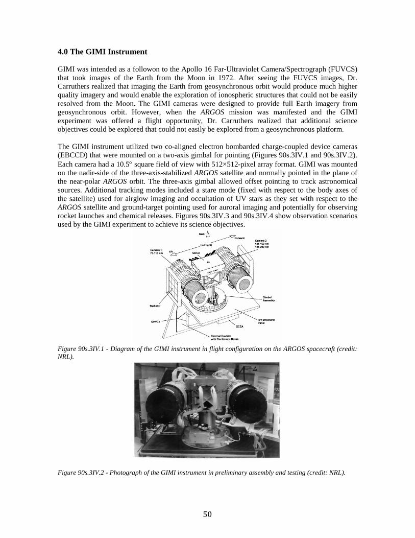
50

4.0 The GIMI Instrument GIMI was intended as a followon to the Apollo 16 Far-Ultraviolet Camera/Spectrograph (FUVCS) that took images of the Earth from the Moon in 1972. After seeing the FUVCS images, Dr. Carruthers realized that imaging the Earth from geosynchronous orbit would produce much higher quality imagery and would enable the exploration of ionospheric structures that could not be easily resolved from the Moon. The GIMI cameras were designed to provide full Earth imagery from geosynchronous orbit. However, when the ARGOS mission was manifested and the GIMI experiment was offered a flight opportunity, Dr. Carruthers realized that additional science objectives could be explored that could not easily be explored from a geosynchronous platform. The GIMI instrument utilized two co-aligned electron bombarded charge-coupled device cameras (EBCCD) that were mounted on a two-axis gimbal for pointing (Figures 90s.3IV.1 and 90s.3IV.2). Each camera had a 10.5° square field of view with 512×512-pixel array format. GIMI was mounted on the nadir-side of the three-axis-stabilized ARGOS satellite and normally pointed in the plane of the near-polar ARGOS orbit. The three-axis gimbal allowed offset pointing to track astronomical sources. Additional tracking modes included a stare mode (fixed with respect to the body axes of the satellite) used for airglow imaging and occultation of UV stars as they set with respect to the ARGOS satellite and ground-target pointing used for auroral imaging and potentially for observing rocket launches and chemical releases. Figures 90s.3IV.3 and 90s.3IV.4 show observation scenarios used by the GIMI experiment to achieve its science objectives.

Figure 90s.3IV.1 - Diagram of the GIMI instrument in flight configuration on the ARGOS spacecraft (credit: NRL).

Figure 90s.3IV.2 - Photograph of the GIMI instrument in preliminary assembly and testing (credit: NRL).

51

Figure 90s.3IV.3 - Diagram illustrating the observing geometry of the GIMI experiment for observing airglow and stellar occultations. GIMI camera #1 was used for sunlit side observations and camera #2 was used for dark side observations (credit: NRL).

Figure 90s.3IV.4 - The detailed viewing geometry for stellar occultation observations (credit: NRL). Camera number 1 was sensitive in the 75-110 nm wavelength range and was intended to monitor the 83.4 nm emission line of O+ on the sunlit side of the Earth and to monitor the 91.1 nm line produced by radiative recombination of O+ ions and electrons on the night-side of the Earth. Camera number 1 had an effective focal ratio of f/2.5 with no Schmidt corrector but instead used an annular aperture to reduce the spherical aberration from the spherical primary mirror. Camera number 2 was sensitive simultaneously in the 131-160 and 131-200 nm wavelength ranges and was designed to image the night-side ionosphere in the 135.6 nm emission line of atomic oxygen and the NO emission near 190 nm. The upper two-thirds of the photocathode in camera number 2 was coated with KBr and was sensitive in the wavelength region below 160 nm. The lower third of the photocathode was coated with CsI to be sensitive below 200 nm. Camera number 2 used an f/1 Schmidt optical system for focusing and included a heated SrF2 Schmidt corrector so its effective f-

52

number was higher than the f-number of camera number 1. Heating the SrF2 Schmidt corrector to 90 C caused the short wavelength cut-off to shift from the nominal (room-temperature) value of 127 nm to 132.5 nm so that the bright emission line from atomic oxygen could be eliminated. The estimated sensitivities are shown in Figure 90s.3IV.5.

Figure 90s.3IV.5 - Preliminary estimates of the sensitivities of the two GIMI cameras. These are the products of the filter and/or corrector plate transmission, the mirror reflectance, and the photocathodes quantum efficiency for each camera, and assuming that all resulting photoelectrons are detected and counted by the electronics (credit: NRL) The GIMI cameras used opaque photocathodes deposited on the curved Schmidt focal surface (Carruthers et al. 2002). As a result, the quantum efficiency of the GIMI cameras was approximately 100%. However, this required that the emitted photoelectrons be electromagnetically focused. The GIMI cameras included large permanent magnet solenoids that provided uniform axial magnetic fields. The two cameras used oppositely oriented magnets so that the net dipole moment would be minimized and the magnetic torques caused by the interaction between the GIMI magnetic dipoles and Earth’s field exerted on the satellite would be reduced to manageable proportions. The photoelectrons emitted at the photocathode would spiral about the magnetic field-lines in the solenoids and would be accelerated from the photocathodes to the charge-coupled devices (CCDs) by a large ~15 KV electric field. The accelerating potential was adjusted so that the photoelectrons would make approximately one spiral about the magnetic field lines before impacting the CCDs. Since CCDs are generally sensitive to visible and near infrared radiation, the GIMI CCDs were overcoated with a layer of aluminum that reflected all light. However, the accelerated photoelectrons would easily penetrate the aluminum layer with the loss of ~6 KV of energy and enter the CCD silicon where they would generate an electron/hole pair for every 2.5 eV of excess kinetic energy. Thus, each photoelectron would produce ~3000 hole-electron pairs, so that individual photoelectrons could be counted against the nominal thermal background of the CCD. The CCDs were cooled, using thermoelectric coolers, to remove the heat associated with the photoelectron impacts and to lower the CCD read and thermal noise. The waste heat from the thermoelectric coolers was transmitted via heat pipe to radiators shown in Figure 90s.3IV.1. 5.0 Key Experiment Results The GIMI instrument on ARGOS was successfully initialized and began operations during the week of May 16, 1999, with images being obtained from both cameras (Carruthers & Seeley 1999). Several anomalies were encountered and overcome before normal operations could commence. On June 8, 1999 the ARGOS spacecraft went into sunsafe attitude mode and all the instruments (including GIMI) were powered down. After ARGOS sunsafe was resolved camera number 1

53

encountered difficulties as indicated by its telemetry readings that were never fully resolved. Camera number 2, on the other hand, returned from sunsafe to normal operations and began taking a series of images of night-time observations of airglow and stellar occultations. Here are two highlights of the GIMI science mission. First observations of ionospheric bubbles from space. Figure 90s.3IV.6 shows images of the ionosphere in the O+ line of oxygen at 135.6 nm. In the first panel, a uniform ionosphere lacking ionospheric bubbles, or irregularities, is shown. In the second image, features that can be identified as "bubbles" can be discerned. The images also show the trails of stars as the cameras were in the staring mode with their field-of-view fixed with respect to the satellite body axes. In Figure 90s.3IV.7, another GIMI image containing ionospheric bubbles has been further analyzed to convert the imagery into physical units using the LORAAS data from the HIRAAS experiment. These bubbles were observed looking northward near the Hawaiian Islands. The panel at the right contains scintillation measurements made at L-band frequencies (1.5 GHz) using the USAF Scintillation Network Decision Aid (SCINDA) site at Mauna Kea, Hawaii. The rectangle at the top of the image indicates scintillation on the GPS signals of satellites with lines-of-sight from Mauna Kea that passed through the GIMI field-of-view.

Figure 90s.3IV.6 – The GIMI experiment on ARGOS observed atmospheric irregularities near the F-region in a neutral oxygen emission line during August 1, 1999 in nightglow measurements. The ionospheric bubble structures can be modeled using numerical MHD techniques (credit: NRL).

Figure 90s.3IV.7- A second bubble image from observations made on July 12, 1999 at 12:47:27 UT. The image at the left has been calibrated using coincident LORAAS data (see the HIRAAS Chapter in this history) and converted to peak electron density in units of 106 cm-3. The horizontal ranges at the tangent point are indicated above and below the image and the tangent latitude is indicated at the right of the image; these distances indicate that the bubbles were most likely beyond the tangent point and so the image contrast is

54

reduced. This interpretation is consistent with the image at the right. The observations occurred over the Central Pacific Ocean overhead of Mauna Kea, Hawaii. The panel at the right shows observations made using the GPS receiver located at the USAF SCINDA site atop Mauna Kea. The heavy black rectangle indicates satellite lines-of-sight from Mauna Kea that pass through the GIMI field-of-view. The fluctuations indicate the presence of scintillation associated with ionospheric bubbles (credit: NRL). First observation of the UV emission from a meteor. Another, this time unexpected, result from the GIMI experiment is shown in Figure 90s.3IV.8. GIMI observed the UV image of a meteor entering the Earth's atmosphere during the Leonid meteor shower during November 1999. Such a UV image had never been obtained before by ground-based observers because the Earth's atmosphere blocks the descending UV photons that are produced in the hot plasma produced during meteor atmospheric entry. The most likely emission source was estimated to be nitric oxide (NO) produced by dissociation of molecular nitrogen and its subsequent reaction with atomic oxygen, producing emission in the 190-200 nm wavelength range.

Figure 90s.3IV.8 - On November 18, 1999 GIMI recorded a meteor entering the Earth's atmosphere. This was the first known image in the ultraviolet of such an event. This image was taken as GIMI was observing the atmosphere during the Leonid meteor shower in November 1999 and shows the image of the meteor trail in the wavelength range 131-200 nm (credit: NRL). 6.0 Legacy The few images from the GIMI instrument increased interest in UV imagery, especially at very high sensitivity, for characterizing the nighttime ionosphere. The potential to see ionospheric bubbles had been pointed out prior to the launch of GIMI but instruments prior to GIMI were not sensitive enough to make the observations. The use of heated strontium fluoride filters and photocathodes was copied by the Tiny Ionospheric Photometer (TIP) instruments on the Constellation Observing System for Meteorology, Ionosphere, and Climate (COSMIC) that set a new standard for sensitivity to UV airglow (Anthes et al., 2008; Dymond et al., 2009). Annular aperture Schmidt cameras with heated fluoride windows are being designed to meet operational ionospheric imaging needs of the DoD. The concept of imaging the Earth’s ionosphere from geosynchronous orbit instigated by Carruthers’ observations is still being pursued today.

55

References: 90s.3IV: ARGOS PART IV: The Global Imaging Monitor of the Ionosphere (GIMI) Experiment Anthes, R. A., P. A. Bernhardt, Y. Chen, L. Cucurull, K. F. Dymond, D. Ector, S. B. Healy, S.-P.

Ho, D. C. Hunt, Y.-H. Kuo, H. Liu, K. Manning, C. McCormick, T. K. Meehan, W. J. Randel, C. Rocken, W. S. Schreiner, S. V. Sokolovskiy, S. Syndergaard, D. C. Thompson, K. E. Trenberth, T.-K. Wee, N. L. Yen, and Z. Zeng, “The COSMIC/FORMOSAT-3 Mission: Early Results”, Bull. Amer. Meteor. Soc., 313-333, DOI:10.1175/BAMS-89-3-313 (2008)

Carruthers, G.R. and Seeley, T.D. “Global Imaging Monitor of the Ionosphere (GIMI) an ultraviolet

ionospheric imaging experiment for the ARGOS satellite”, in Instrumentation for planetary and terrestrial atmospheric remote sensing (Vol. 2831 of Proceedings of the S.P.I.E.), p.322 (1992)

Carruthers, G.R. and Seeley, T.D. “Global Imaging Monitor of the Ionosphere (GIMI): a Far-

Ultraviolet Imaging Experiment on ARGOS”, in Ultraviolet Atmospheric and Space Remote Sensing: Methods and Instrumentation (Vol. 2831 of Proceedings of the S.P.I.E.), p.65 (1996)

Carruthers, G.R. and Seeley, T.D. “The Global Imaging Monitor of the Ionosphere (GIMI) on the

Advanced Research and Global Observation Satellite (ARGOS): Quick Look Results”, in Ultraviolet Atmospheric and Space Remote Sensing: Methods and Instrumentation II (Vol. 3818 of Proceedings of the S.P.I.E.), p.160 (1999)

Carruthers, G.R., Seeley, T.D., Shephard, K.K. and Finch, M.A. “Pre-Flight and In-Flight

Calibrations of the Global Imaging Monitor of the Ionosphere (GIMI) on the Advanced Research and Global Observation Satellite (ARGOS)”, in Optical Spectroscopic Techniques, Remote Sensing, and Instrumentation for Atmospheric and Space Research IV (Vol. 4485 of Proceedings of the S.P.I.E.), p.316 (2002)

Dymond, K. F., S. A. Budzien, C. Coker, and D. H. Chua, “On-orbit Calibration of the Tiny

Ionospheric Photometer on the COSMIC/FORMOSAT-3 Satellites”, Solar Physics and Space Weather Instrumentation III. Edited by Fineschi, Silvano; Fennelly, Judy A. Proceedings of the SPIE, 7438, pp. 743814-743814-11, doi: 10.1117/12.825316 (2009)

56

90’s.4: EUV Solar Physics sounding rockets at NRL (1975-2005)

Contributed by Clarence M. Korendyke

1.0 Overview After the Skylab mission and instrumentation (Sec. 70s.2), NRL scientists developed the next generation of ultraviolet/extreme ultraviolet (UV/EUV) solar sounding rocket payloads. These payloads had <1 arc-second resolution and were specifically developed to have high spatial, spectral and temporal resolution. They recorded the evolution and physical characteristics of the solar atmosphere via spectroscopy with higher spatial resolution than had ever been achieved at wavelengths inaccessible from the ground. The payload spatial resolution was comparable to the highest resolution routinely available from ground based observatories at the time and enabled a new series of discoveries of the solar atmosphere. The most remarkable of these discoveries was the first observation in 1975 of small scale, transient, explosive events visible in the spectral line profiles of the C IV emission line doublets. These high velocity transient events showed for the first time the importance of small scale and rapid physical processes in the solar atmosphere. Small scale, sporadic physical processes have now been recognized as being the dominant processes governing the flow of mass and energy within the solar atmosphere. Other discoveries of great importance from the first Very high Angular resolution ULtraviolet Telescope (VAULT) flight were the long strands visible in Lyman-α prominences and the rapid evolution of the upper chromosphere with structure lifetimes of <90 seconds. Exploring and understanding small scale processes in the upper solar atmosphere remains an essential focus of currently operating and planned missions in solar physics. Results were documented in over 140 publications. A subset are cited in the references. Between 1975 and 2005, NRL developed and successfully flew two high spatial resolution sounding rocket payloads. The first of these was flown multiple times. This payload was the High Resolution Telescope and Spectrograph (HRTS) developed by NRL/SSD researchers Guenter Brueckner, John-David Bartoe and Dianne Prinz. Since its first flight in 1975, HRTS recorded high quality ultraviolet spectra of the Sun on ten rocket flights and during extended operations on the Space Shuttle Spacelab 2 mission in 1985. The HRTS payload obtained high spatial resolution (<1 arc-second) EUV spectra and spectroheliograms over a large field of view. The second much more recent payload, the VAULT was developed by NRL/SSD researchers, Clarence Korendyke and Angelos Vourlidas and has flown successfully twice. This payload obtained spectrally pure observations of the Lyman-α emission lines with ~0.33 arc-second resolution on the solar disk, another ground-breaking achievement in high spatial resolution EUV observations. A photograph of the VAULT 1 launch at the White Sands Missile Range (WSMR) is given in Figure 90s.4.1. The typical observation time available during a HRTS or VAULT flight was roughly 300 seconds. The payloads were launched from White Sands Missile Range Launch Complex 36 on NASA provided Black Brant rockets manufactured by Bristol Aerospace. To achieve additional altitude, the launch complement included a Terrier Booster. A nominal payload stackup is shown in Figure 90s.4.2. The NASA Solar Pointing Acquisition and Rocket Control System (SPARCS) provided the necessary payload pointing and stabilization. SPARCS was originally developed by NASA to support the NRL photographic film based solar physics sounding rocket program. This fine pointing system is still in use today. The payloads were launched uprange and recovered using range military helicopters. This essay describes the development and flight of the HRTS and VAULT instrumentation. It gives a general history of the HRTS and VAULT payloads, their development and data sets. The extensive HRTS and VAULT publications in refereed journals describe the scientific results in detail.

57

Figure 90s.4.1 - Photograph of the VAULT 1 launch: May 7, 1999 (credit:NASA).

Figure 90s.4.2 - Payload Configuration stackup from a VAULT flight. Significant components include the experiment section, the telemetry section, the SPARCS section and the recovery section (credit: NASA).

2.0 HRTS sounding rocket program The heritage of the HRTS program lies in the NRL ultraviolet spectrograph on the Skylab Apollo Telescope Mount and its rocket-born predecessors. This spectrograph obtained spectra in the 970-1970Å and 1940-3940Å wavelength regions of a 2" x 60" area of the Sun, see Skylab Essay 70s.2 in this History. Since ground based observations in visible light showed the existence of

58

considerable structure at the arc-second level, the central goal was to design a spectrograph that could simultaneously record an extended ultraviolet spectrum with arc-second resolution. In addition, it would need to be a double-dispersion spectrograph in order to eliminate stray light. This was accomplished by the invention of the tandem-Wadsworth spectrograph by Guenter Brueckner and John-David Bartoe (Bartoe et al., 1975). Dr. Bartoe’s Ph.D. thesis at Georgetown University describes the tandem Wadsworth design and subsequent implementation in the HRTS rocket payload in detail. The spectrograph optical layout is given in Figure 90s.4.3. The first grating collimates light from the slit and disperses the EUV radiation. The mount of this grating is a Wadsworth collimator with the slit located at the EUV focus of the grating. The dispersed EUV radiation is reimaged by a second grating onto a curved film focal plane. The astigmatism is reduced to a very low level because the central rays at each wavelength are both collimated and reimaged at the ideal, normal incidence Wadsworth mount angle. The design produces astigmatic spectra along the whole slit and at all wavelengths within the spectral range. The dispersions of the two gratings are additive obtaining a relatively high dispersion for a modest 2400 line/mm ruling density. The flight spectrograph requirements for the first flight were as follows: (a) wavelength coverage, 1200-1700Å, (b) f/15 telescope feed, (c) resolvable element size at the film plane over the entire wavelength range, 10 x 10 microns (spectral and spatial), and, (d) dispersion, 5Å/mm. All four requirements were shown to be fulfilled by the symmetric tandem Wadsworth spectrograph.

Figure 90s.4.3 - Tandem Wadsworth Spectrograph geometry (Bartoe and Brueckner, 1975) (credit: NRL).

A conventional Cassegrain telescope was then coupled with the tandem-Wadsworth spectrograph to form the sounding rocket payload (see Figure 90s.4.4). Because of the resolution and large format (22x110mm focal plane) required for the detector, photographic film was the only suitable detector available. The Skylab proven Kodak 101 Schumann emulsion was selected. The entire design fit inside a cylinder roughly 270 cm long and 44 cm in diameter as sketched in Figure 90s.4.2. This accommodates a 30 cm f/15 Cassegrain telescope with a focal length of 450 cm and the tandem-Wadsworth spectrograph with a folding mirror for compactness. An Hα visible light system was incorporated to provide real time video images of the UV spectrograph slit jaws for pointing and to record these images photographically for post flight analysis. A roll film camera was developed specifically for the HRTS application. The camera was capable of taking >30 full frames using the Kodak 101 film. A much larger version was developed for the Spacelab 2 application. A UV spectroheliograph slit jaw imaging system was added for later flights.

59

Figure 90s.4.4 - Optical layout of the HRTS sounding rocket payload (Bartoe and Brueckner, 1975). The 30cm Cassegrain telescope fits comfortably within the 17 1/4” skin diameter. The introduction of a folding mirror (M3) in the tandem Wadsworth spectrograph results in a compact spectrograph geometry readily accommodated within the sounding rocket envelope (credit: NRL).

The 1170-1700Å region of the spectrum contains numerous spectral lines and continua that are valuable diagnostics of the temperature minimum region, chromosphere and transition region, which are all important regions for understanding the strong non-radiative heating that maintains the outer solar atmosphere. The temperature minimum region can be studied with the 1600Å continuum. The intensity and velocity patterns in the chromosphere are mapped, for example, by the resonance and intercombination lines of C I near 1560Å and 1613Å, respectively. In the transition region, there are density sensitive line ratios of Si III and O IV in addition to the strong lines of Si IV and C IV. Several weak coronal lines and a strong flare line of Fe XXI complement the primary investigation by providing coronal and flare diagnostics, mostly useful by pointing outside the solar limb. However, the flare line is also useful for disk observations. An example of Hα images and slit spectrograms are given in Figure 90s.4.5.

The sections below describe the results from individual HRTS flights as they were determined at the times of the flights.

Figure 90s.4.5 - HRTS spectra and Hα slit jaw images from the HRTS 3 flight. The explosive events are clearly visible in the C IV emission lines (credit: NASA/NRL).

60

2.1 The First Rocket Flight: July 21, 1975

The first spectra were extremely impressive. The spectra dramatically demonstrated the highly inhomogeneous nature of the chromospheric and transition zone intensity and velocity fields. The pointing of the slit was chosen so that it intersected a sunspot and the quiet solar limb. The first observations of a variety of supersonic phenomena were made: coronal jets, explosive events and sunspot downflows. The high velocity outflows led to the suggestion that they were a potential source for the solar wind. Molecular lines of CO and H2 were discovered in sunspots where they are excited by H Ly fluorescence.

2.2 The Second Rocket Flight: February 13, 1978

For the second HRTS rocket flight, a broadband ultraviolet spectroheliograph was added to view the UV spectrograph slit jaws. The design is similar to the tandem-Wadsworth spectrograph except that the orientation of the two gratings are oriented such that the dispersions of the two gratings cancel rather than add. The bandpass is about 50Å and when centered at 1600Å, the temperature minimum continuum emission dominates the chromospheric emissions on the disk.

The second flight again placed the slit radially through a sunspot and the quiet limb. While waiting in the tower at White Sands, the temperature in the telescope rose beyond its nominal operating range and so it was somewhat out of focus during flight. The spectroheliograph images showed that the majority of emission in the quiet temperature minimum is produced in small grains near the resolution of the instrument. A spectacular example of a repeating 500 km/s coronal jet was found in an undistinguished part of the quiet Sun. Transition region flows of up to 300 km/s were found to extend over a good portion of a major sunspot which contained a large light bridge.

2.3 The Third Rocket Flight: March 1, 1979

The observations of transient high velocity outflows in both previous rocket flights gave considerable support to the notion that they were responsible for the generation of the solar wind. However, because of the small areas of the solar surface sampled, the extrapolation to a global phenomena was a large and uncertain jump. It was decided that a program to perform sequential spatial rasters of a more extended region of the Sun would be very worthwhile. On the third rocket flight the slit was rastered in 2" increments to obtain 6 exposures of a 10" wide region. This sequence was repeated to build up 10 complete rasters and one incomplete raster. By limiting the spectrograph range to 50Å roughly centered on the C IV lines near 1550Å, it was possible to use a smaller but faster ruled grating for an increase in throughput of about a factor of 2. With the slit also opened up by a factor of 2, exposure times of 3 s could be used. While a large number of explosive events (100 km s-1) were observed, none of the high velocity (500 km/s) coronal jets were found. The conclusion was that, although the events were not energetically important, there was possibly enough mass ejected in the explosive events to account for the mass requirements for the solar wind. From the two dimensional profile data obtained in the rasters, it was possible to reconstruct images of the intensity and velocity fields in the chromospheric lines of C I and Fe II and the transition zone lines of C IV as well as intensity images of the temperature minimum continuum. These showed that the quiet transition zone consisted of structures that were essentially extensions of the chromospheric spicules. Simultaneous H observations from Sac Peak showed that the Fe II emissions were produced in the same plasmas responsible for the formation of the spicules seen in the blue wing of H. The Doppler shifts in the ultraviolet lines were less than 3 km/s, an order of magnitude below the velocities inferred from H limb observations. Instead, extremely small regions in the supergranular cell centers were found with blue shifts in the C I lines which

61

indicated flow velocities of about 20 km/s. The time sequences of the C IV images showed that the rare blue shifted structures were generally associated with expulsions and ejections rather than some sort of laminar flow along magnetically confined stream lines. The spectroheliograph was tuned to 1550 Å in order to see transition region structure above the disk. These also suggested the existence of transient ejecta but the stray light from the disk emissions masked many of these weak phenomena.

2.4 The Fourth Rocket Flight: March 7, 1983

The goal of the fourth rocket flight was to observe the fine-scale structure of the solar transition zone and chromosphere at the limb. A curved slit jaw, with a radius of curvature twice that of the Sun, was installed into the spectrograph. In order to eliminate straylight in the spectroheliograph above the limb, a low-reflectance coating for visible light was used on one of the slit jaw surfaces. Further, a mechanism for translating the secondary mirror in flight to achieve the best focus of the telescope was also employed. Pointing and focusing of the experiment were to be controlled from the ground, based on the Hα video downlink. Unfortunately, the telemetry link to the rocket malfunctioned and it was not possible to properly focus the telescope. Nevertheless, profiles of coronal lines of Si VIII, Fe X, XI, and XII were obtained for quiet coronal structures as well as inside a coronal hole for the Si VIII line formed at 9 x 105 K. This is an important data set because it places the limits on the Alfven wave energy flux that is often invoked to explain the acceleration of high speed solar wind streams.

2.5 The Fifth HRTS Rocket Flight: December 11, 1987

The fifth flight was conceived as a dual rocket campaign involving both the HRTS and the American Science & Engineering (AS&E) X-ray rocket payloads. The primary goal was to determine the coronal manifestation, if any, of the coronal jets and explosive events observed in the HRTS transition region spectra. After a frustrating series of problems with the rocket guidance system, the two rockets were launched within a half hour of each other. The AS&E payload returned a series of exposures of the full disk through several filter combinations. The HRTS performed a large area raster in the spectral region near 1550 Å, which includes lines of C I, Fe II and C IV. Coordinated observations were also obtained by the Big Bear Solar Observatory (video magnetograms) and the Kitt Peak Observatory (He 10830 spectroheliograms and magnetograms). Explosive events are not well correlated to X-ray bright points but tend to occur at the borders of the supergranular network. It is possible that they are related to the coalescence and cancellation of magnetic flux which is known to occur in those regions. There also seems to be some tendency for the explosive events to occur where the X-ray emission is relatively weak.

2.6 The Sixth Rocket Flight: November 20, 1988

The coronal jets and explosive events observed with the HRTS have been suggested as potential sources of the solar wind. The target for this flight was a coronal hole. EUV spectra obtained by others suggested a relative blueshift in coronal holes on the disk but these spectra lack an absolute wavelength calibration. The HRTS spectra can be referenced to narrow chromospheric lines to determine a near absolute velocity scale. The sixth rocket flight was successful in observing a well-defined coronal hole on the disk. The C IV spectra show that there is a significantly greater probability of outflows inside the coronal hole. Approximately 26% of the coronal hole shows blueshifts and the average blueshift velocity is 5 km/s. Nevertheless, the average velocity in the coronal hole is a 2 km/s downflow.

In addition to the coronal hole, an emerging active region and emerging flux regions were within the field of view of the slit rasters. A map of the positions of the explosive events in these regions

62

showed a greatly enhanced population. In the emerging active region, the explosive events outlined the borders of high magnetic flux regions and, in particular, the magnetic neutral line. In the emerging flux region, the explosive events occurred along three well defined lines, apparently again demarcating the neutral line of the emerging flux and the boundary between the new flux and the preexisting flux. Combined with the strong evidence in the Spacelab 2 data that explosive events were associated with emerging flux, it was proposed that the mechanism driving the explosive events was magnetic reconnection, whether in the emerging flux regions or in the majority of the explosive events which have, as yet, no defined relationship with magnetic signatures. It was further proposed that the majority of explosive events are the result of the process of magnetic cancellation of photospheric flux elements observed in the Big Bear video magnetograph and identify this process as magnetic reconnection. By equating the velocity of the explosive events with the local Alfven speed and measuring the density with density sensitive line ratios of O IV, a magnetic field strength of 20 gauss is derived for the reconnection volume.

2.7 The Seventh Rocket Flight: November 21, 1990

The seventh rocket flight of the HRTS occurred jointly with a launch of the AS&E X-ray telescope to obtain nearly simultaneous X-ray images and ultraviolet spectra of a flare-producing active region. The payloads were ready for flight from White Sands in early June but the Sun remained inactive for a period of about 2 months at the peak of the solar cycle. Finally, a flaring active region appeared with a tongue of one magnetic polarity intruding into plage of the opposite magnetic polarity. Flares occurred along this tongue throughout the day. The two rockets were fired within a half hour of each other and both observed a solar flare. The HRTS spectra showed that the core of the hot flare, seen in Fe XXI 1354Å (10 MK), was only a few arc-seconds in extent and bridged the neutral line on one side of the intruding polarity. Explosive events were also observed on both sides of this tongue. The first ultraviolet spectra of an Ellerman bomb were obtained. These showed extremely wide profiles in transition zone lines with velocities of up to 200 km/s. The first concrete association of an explosive event with changes in the photospheric magnetic configuration was found, in support of the idea that the explosive events are the direct result of magnetic reconnection.

2.8 The Eighth Rocket Flight: August 24, 1992

On August 24, 1992 the HRTS was launched on a Black Brant rocket to observe an active region at the solar limb in the ultraviolet with 1 arc-second resolution. The instrument telescope was changed to a Gregorian configuration. In order to reduce stray light at the spectrograph slit, a disk occulter was placed at the prime focus of the primary mirror and a Lyot stop was employed as well. The spectrograph covered the 1850-2670Å wavelength range which includes strong lines of Fe II, Si II, Si III, C III and Fe XII spanning the 0.01 – 1.0 MK temperature range. The spectrograph slit was curved to conform to the solar limb and was successively stepped above the limb in 0.10 R increments. The spectroheliograph included a new narrow band filter to image the C IV emissions near 1550Å.

63

Figure 90s.4.6 - HRTS 8 spectra and spectroheliograms. Spectra taken above the limb showed remarkable structure. The flight spectroheliograms sequence captured a C IV surge in progress at the limb (credit: NRL).

Representative images and spectra from the flight are given in Figure 90s.4.6. Above the limb, the C IV spectroheliograph images showed that the active region transition zone consists of a variety of threads, twisted threads, disconnected threads and point-like objects that extend high above the limb and bear more resemblance to a prominence than to typical coronal loop structures. On the disk, the active region seen in C IV consists of diffuse structures, small loops and bright points. The quiet sun C IV structures on the disk are generally elongated, suggesting the extensions of the spicules but the fine, high-contrast structures seen above the limb were not apparent.

The characteristics of the coronal line profiles observed in the ultraviolet spectra show a marked contrast to those of the chromospheric and transition region lines. The coronal lines reveal only slowly varying changes in intensity as a function of position while the chromospheric and transition region lines show considerable structure at the 1 arc-second resolution of the instrument. Velocities in the coronal lines are uniformly low whereas the chromospheric and transition region lines show strong variations. Supersonic velocities as high as 70 km/s are seen in loop structures and may be related to the high speed downflows seen in sunspot spectra on the disk in previous HRTS flights. Density sensitive line ratios of Si III/C III and Fe XII are available to determine pressures and fill factors.

2.9 The Ninth Rocket Flight: April 18, 1995

For the ninth flight, HRTS was reconfigured to observe the near-UV lines of Mg I and Mg II near 2800Å. This flight studied the variations in the Mg I and II profiles to understand their contribution to observed changes in the solar irradiance. This was accomplished by rastering the slit across a sunspot, a plage and regions of the quiet Sun. The spectra were used to refine calculations of the Mg II index during the solar cycle and provided fundamental evidence of the importance of small spatial scales in this part of the atmosphere. The spectroheliograph system was modified to incorporate four narrow bandpass, EUV filters. These successfully isolated the C IV emission and showed bright loops along the active region magnetic neutral line. The payload was successfully launched on April 18, 1995.

64

Figure 90s.4.7 - Mg I and II spectra from HRTS 9. The spectra show the emission in active regions at the core of the deep absorption lines. The spectra were the highest spatial resolution obtained at the time (credit: NRL). 2.10 The Tenth rocket flight: September 30, 1997 HRTS was successfully launched on Sept. 30, 1997. For this tenth rocket flight, the instrument consisted of a 30cm Cassegrain telescope and a three element focal plane package. The central focal plane instrument was a tandem Wadsworth spectrograph with wavelength coverage in two bands (120-140nm and 150-170nm) with a resolution of 50mÅ. The reflective spectrograph slit jaws are imaged with an intermediate bandpass UV spectroheliograph and with a visible H-alpha slit jaw imaging system. As on the previous flight, four (20 Å FWHM) filters were used in the spectroheliograph to obtain images with central wavelengths at 1540, 1550, 1560 and 1600 Å. The spectra and images were recorded on photographic film. The instrument was successfully pointed and focussed in flight. 1 arc-second spatial resolution was achieved in all the images.

The observation target for the mission was the north polar coronal hole. During the prime mission, the 900" long slit was moved over the surface of the Sun to obtain a 10" wide raster with 2" steps. The slit was positioned nearly radially with 100" above the northern limb of the Sun. A wide range of exposures was taken to observe a wide variety of bright and faint lines. A series of spectroheliograph and H-alpha images were taken of the spectrograph slit jaws to reference the slit location. An excellent collaborative data set was obtained at Kitt Peak Observatory (chromospheric and photospheric magnetograms), Big Bear Solar Observatory and University of Hawaii. The space based collaborative observing campaign included instruments on other spacecraft: the Solar X-ray Telescope (SXT) on Yohkoh, and the Michelson Doppler Imager (MDI), the Extreme-ultraviolet Imaging Telescope (EIT), the Coronal Diagnostics Explorer (CDS) imaging spectrometer, and the Solar Ultraviolet Measurements of Emitted Radiation (SUMER) imaging spectrometer on the Solar & Heliospheric Observatory (SOHO). The slit spectra show an interesting collection of explosive events in C IV. The spectroheliograph images show C IV loop-like structures near the limb.

The flight also was the first scientific flight of the new digital attitude control system produced by the Lockheed Martin SPARCS group at the White Sands Missile Range. The system utilizes fast, programmable digital control of the payload. The previous problem of ground loop noise on the

65

shielded sensor lines was entirely eliminated by the incorporation of a fiber optic sensor data line. The performance of this new system was superb. Acquisition occurred within 30 seconds of opening the aperture door. The noise on the sensor output lines was 0.05 arc-seconds. The stability over the entire flight was 1.5 arc-seconds peak to peak. The stability of the pointing over a typical 10 second exposure was 0.2 arc-seconds peak to peak and <0.1 arc-seconds peak to peak for a typical 1 second exposure. This enhanced pointing stability enables very high spatial resolution solar images to be obtained from a sounding rocket platform.

3.0 The VAULT Instrument

VAULT is a sounding rocket payload designed, fabricated, and flown by the Naval Research Laboratory Solar Physics Branch. The payload was designed and built by Clarence Korendyke and Angelos Vourlidas. The payload fully exploited the heritage of the HRTS to achieve even higher spatial resolution at the hydrogen Lyman α line. The VAULT instrument was successfully launched twice. Two major scientific results of the program were the discovery of highly filamentary structures within prominences and the rapid evolution of structures in the upper chromosphere. These structures were nearly completely recycled in ~90 seconds.

The principal components of VAULT are shown in Figure 90s.4.8. The instrument and in-flight technical performance are described in Korendyke et al. (2001). VAULT uses an excellent optical quality (λ/16 rms at 121.5 nm), 30 cm diameter telescope followed by a zero dispersion spectroheliograph to obtain 0.33 arcsecond spatial resolution UV images. The solar radiation passing through the field stop is collimated and dispersed by G1, reflected by a single folding mirror and recombined by G2. The G1 and G2 grating configuration was selected to obtain a UV solar image with minimal geometric blur (<5 microns, 0.07 arcsecond, predicted by a ray trace), moderate bandpass (15.0 nm at Lyman-α) and high efficiency (~13%). The solar image is projected onto a lumogen coated, 2048x3072, 9 micron pixel KAF-6301 Kodak CCD. The CCD UV quantum efficiency (>10%), linearity and dynamic range are substantially improved over the 101 film used in NRL's HRTS flights. The throughput allows short exposure times (1s) even with a plate scale of 72 microns/arcsecond.

Figure 90s.4.8 - VAULT opto-mechanical layout (credit: NRL).

The first VAULT flight, on May 7, 1999, outfitted with a Lyman-α spectroheliograph obtained the highest resolution (0.33 arcsecond) solar images from space to date. An analysis of the VAULT Lyman-α and the Transition Region and Coronal Explorer (TRACE) 17.1 nm images revealed a high correlation between the fine-scale structures in the two regimes but a large discrepancy in their emission level. This result placed important constraints on coronal heating mechanisms. Also, the comparison of TRACE and VAULT Lyman-α images has led to an improved method for the removal of the continuum contribution from the TRACE Lyman-α images.

66

The second VAULT flight, on June 14, 2002 achieved higher sensitivity and obtained the highest resolution (0.33 arcsecond) solar images from space to date. Figure 90s.4.9 shows the complex filamentary structures observed during the second flight. Angelos Vourlidas adjusted the pointing in mid-flight to produce spectacular off-limb images. A number of publications have been written based on the analysis of the VAULT data and the observations of a large campaign using ground and space-based telescopes.

Figure 90s.4.9 - VAULT image in Lyman-α after flat field correction and wavelet enhancement. The image is a composite of two pointing positions during the 2nd flight (600x256 arc-seconds). The large field of view of the VAULT CCD (384 x 256 arc-seconds) captured a variety of solar structures, including an active region and off-limb loops, simultaneously (credit:NASA/NRL). 4.0 Field Operations Rocket field operations were memorable events within the life of the NRL/SSD Solar Physics Branch. The typical duration of a field trip was about three weeks. The team aligned and focused the payload at the laboratory. The payload operations at White Sands Missile Range included a full suite of payload tests (pre-vibration test, spin balance and vibration testing). The team also conducted pre-launch flight simulation testing using a large Heliostat for several days. The payload was launched from LC-36 and recovered with helicopters. Experiment teams typically sent several members to help with the recovery. Over the years, the launch teams stayed on-base at WSMR, in El Paso and in Las Cruces. A memorable tradition was Mexican style dinners at La Posta and steak dinners at the Double Eagle in old Mesilla. In Las Cruces, the team enjoyed eating at Casa Luna, the Cattle Baron, Luby’s and many other places. During rare days off on the weekend, the team visited the White Sands National Monument, enjoyed hiking in the Organ mountains and took the occasional trip to Juarez. Launch days were filled with activity. To achieve thermal isolation, NRL has always evacuated the payloads at the pad. Vacuum operations would start several days ahead of time to reach an adequate vacuum on launch day. Several team members stayed with the payload to monitor vacuum levels the day before launch. The T-times were set to be as close to local solar noon as allowed by the SPARCS performance parameters. The day before launch a set of solar target images was obtained and nominal payload pointings were calculated. For the HRTS launches, solar images were taken and processed with a ground-based Hα photographic telescope station located at LC-35. The objective lens of this telescope was a Zeiss lens donated by Guenter Brueckner. The lens was used by Guenter Brueckner when he was a boy. On launch day, the team arrived at the

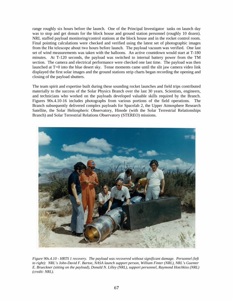
67

range roughly six hours before the launch. One of the Principal Investigator tasks on launch day was to stop and get donuts for the block house and ground station personnel (roughly 10 dozen). NRL staffed payload monitoring/control stations at the block house and in the rocket control room. Final pointing calculations were checked and verified using the latest set of photographic images from the Hα telescope about two hours before launch. The payload vacuum was verified. One last set of wind measurements was taken with the balloons. An active countdown would start at T-180 minutes. At T-120 seconds, the payload was switched to internal battery power from the TM section. The camera and electrical performance were checked one last time. The payload was then launched at T=0 into the blue desert sky. Tense moments came until the slit jaw camera video link displayed the first solar images and the ground stations strip charts began recording the opening and closing of the payload shutters. The team spirit and expertise built during these sounding rocket launches and field trips contributed materially to the success of the Solar Physics Branch over the last 30 years. Scientists, engineers, and technicians who worked on the payloads developed valuable skills required by the Branch. Figures 90s.4.10-16 includes photographs from various portions of the field operations. The Branch subsequently delivered complex payloads for Spacelab 2, the Upper Atmosphere Research Satellite, the Solar Heliospheric Observatory, Hinode (with the Solar Terrestrial Relationships Branch) and Solar Terrestrial Relations Observatory (STEREO) missions.

Figure 90s.4.10 - HRTS 1 recovery. The payload was recovered without significant damage. Personnel (left to right): NRL’s John-David F. Bartoe, NASA launch support person, William Finter (NRL), NRL’s Guenter E. Brueckner (sitting on the payload), Donald N. Lilley (NRL), support personnel, Raymond Hotchkiss (NRL) (credit: NRL).

68

Figure 90s.4.11 – NRL’s Donald N. Lilley (lower right) and Dianne Prinz (NRL) (orange shirt) installing a skin on a solar physics sounding rounding rocket payload (credit: NRL).

Figure 90s.4.12 - HRTS 7 launch team (from left to right). Robert Moye (ARTEP), Thomas Spears (NRL), Dennis Socker (NRL), Clarence Korendyke (NRL), Frank Lau (NASA Wallops Flight Facility), David Roberts (NRL), James Smith (ARTEP) (credit: NRL).

69

Figure 90s.4.13 - VAULT 1 launch team from left to right: Ronen Feldman (ARTEP), Thomas Spears (NRL), Clarence Korendyke (NRL), Robert Moye (ARTEP), David Roberts (NRL), Angelos Vourlidas (NRL), John Moser and James Smith (ARTEP) (credit: NRL). References: 90s.4: EUV Solar Physics sounding rockets at NRL (1975-2005)

Bartoe, J.-D.F., Brueckner, G.E.: 1975, Journal of Optical Society of America, 65, 13.

Korendyke, C. M.; Vourlidas, A.; Cook, J. W.; Dere, K. P.; Howard, R. A.; Morrill, J. S.; Moses, J. D.; Moulton, N. E.; Socker, D. G.: 2001, Solar Physics, v. 200, Issue 1/2, p. 63-73.

“Lines of H2 in Extreme Ultraviolet Solar Spectra,” Jordan, C., Brueckner, G.E., Bartoe, J.-D.F., Sandlin, G.D., and VanHoosier, M.E. 1977, Nature, 270, 326. “The Energy Balance and Pressure in the Solar Transition Zone for Network and Active Region Features,” Nicolas, K.R., Bartoe, J.-D.F., Brueckner, G.E., and VanHoosier, M.E. 1979, Ap. J., 233, 741. “The Energy Balance and Pressure in the Solar Transition Zone for Network and Active Region Features,” Nicolas, K.R., Bartoe, J.-D.F., Brueckner, G.E., and VanHoosier, M.E. 1979, Ap. J., 233, 741. “Observations of High-Energy Jets in the Corona Above the Quiet Sun, the Heating of the Corona, and the Acceleration of the Solar Wind,” Brueckner, G.E., and Bartoe, J.-D.F. 1983, Ap. J., 272, 329.

70

“Transition Zone Flows Observed in a Coronal Hole on the Solar Disk,” K. P. Dere, J.-D.F. Bartoe, G. E. Brueckner, F. Q. Recely, 1989, Astrophys. J. (Letters), 345, L95. “Explosive Events and Magnetic Reconnection in the Solar Atmosphere,” K. P. Dere, J.-D. F. Bartoe, G. E. Brueckner, J. A. Ewing, and P. A. Lund, 1991, JGR, 96, 9399. “Solar Fine Scale Structures in the Corona, Transition Region and Lower Atmosphere,” D. Moses, J. W. Cook, J.-D. F. Bartoe, G. E. Brueckner, K. P. Dere, D. F. Webb, J. M. Davis, J. W. Harvey, F. Recely, S. F. Martin, and H. Zirin, 1994, Ap J., 430, 913.

“Ultraviolet observations of the structure and dynamics of an active region at the limb”, Korendyke, C.M., Dere, K.P., Socker, D.G., Brueckner, G.E., and Schmieder, B., 1995, Ap J., 443, 869.

71

90’s.5: The Mountain Wave Forecast Model (MWFM)

Contributed by Stephen D. Eckermann

1.0 Introduction For more than half a century, the Department of Defense (DoD) has relied on high-altitude long-endurance (HALE) reconnaissance aircraft to fulfill its mission. First developed in the mid-to-late 1950s, the United States Air Force (USAF) still makes extensive operational use of its fleet of U-2 planes. More recently, USAF (and now the Navy) deploys Global Hawk, a HALE Unmanned Aircraft System (UAS). HALE aircraft cruise twice as high as conventional aviation, typically at ~60,000-70,000 feet (FL600-700, or heights of ~20 km). U-2 flights can last up to 6-8 hours, whereas Global Hawk can remain airborne for up to 42 hours, which, given air speeds ~150-200 ms-1, provides nearly global range. For these reasons, in 2008 the Navy selected Global Hawk as the candidate aircraft to provide future global maritime surveillance and reconnaissance capabilities under its Broad Area Maritime Surveillance (BAMS) program. HALE aircraft have lightweight broad-winged designs that both maximize lift and minimize extraneous weight, enabling them to reach stratospheric altitudes. These properties make them both aerodynamically and structurally vulnerable to severe turbulence at altitude. Since the stratosphere is very dry, cloud-related sources of turbulence are absent and only clear-air turbulence (CAT) can occur. Because of the stratosphere’s stable temperature structure, turbulence levels are generally very low, and so it is often mistakenly assumed that severe CAT never occurs at HALE UAS cruise altitudes. In fact (though much U-2 flight history remains classified) it has emerged that stratospheric CAT (stratCAT) was implicated in the loss of a U-2 over Korea and in numerous other mishaps (Allen 2003). Half a century of accumulated U-2 pilot experience has revealed that, away from deep convective tropical weather, HALE aircraft encounters with severe stratCAT usually occur near mountain ranges (e.g., Ehernberger 1987; Stefanutti et al. 1999). The only plausible connection between underlying orography and severe in-flight CAT in the dry, stable middle stratosphere is via direct propagation of mountain-generated gravity waves (mountain waves) from the ground to the stratosphere, where they break, much like ocean waves on the shore, and generate turbulence. 2.0 Meeting the Science Challenge: the Mountain Wave Forecast Model (MWFM) Thus, global forecasts of mountain-wave stratCAT are required for HALE airframes, but current operational numerical weather prediction (NWP) systems cannot provide them. Finite computational resources force NWP models to run at coarse space-time resolutions that do not resolve the full spectrum of gravity waves forced by flow over orography, nor the smaller turbulent layers that form within breaking waves to yield stratCAT. Projected future increases in computing power offer no prospect of solving this fundamental resolution constraint. Thus novel new forecasting approaches are required. The issue became pressing in the late 1980s and early 1990s when NASA used an instrumented extended-range U-2 (ER-2) to research the newly discovered large unexplained losses of stratospheric ozone over Antarctica (Farman et al. 1985). The ER-2 took off and landed from the tip of South America in notoriously harsh local winter weather conditions associated with the high Andes Mountains and the Drake Passage. It then flew into polar night along the high mountain ranges of the Antarctic Peninsula, deep into the harsh remote Antarctic environment, where few, if any emergency landing or rescue facilities were present (Tuck et al. 1989). Avoiding stratCAT

72

therefore became paramount in flight planning, especially when it was discovered that the ER-2 was regularly intercepting large-amplitude mountain waves over Antarctica (Gary 1989; Bacmeister et al. 1990). In response to this need, Dr. Julio Bacmeister, having recently joined the Space Science Division in February 1992, developed a simple diagnostic forecasting algorithm, based on blowing forecast winds over simplified decompositions of the Earth’s major topographic features (see Figure 90s.5.1), then propagating forced mountain waves upwards through the predicted background atmosphere using simple analytical wave equations. Despite its simplicity, the model, which has subsequently become known as version 1 of the Mountain Wave Forecast Model (MWFM-1), showed skill in predicting occurrences of mountain wave-induced stratCAT encountered by the ER-2 (Bacmeister et al. 1994).

Figure 90s.5.1 - (a) raw topographic elevations over the western USA from the GTOPO30 digital elevation database. Red boundary box shows domain used during operational MWFM-1 and MWFM-2 forecasting for NASA’s MidCiX experiment during April-May, 2004, in which the HALE WB-57 aircraft flew science missions out of Ellington Field. (b) One of the MWFM ridgelet databases formed from ridge-based decomposition of topography for region (a). Overlapping ridges are sorted in the plot such that higher ridgelets are plotted beneath shorter ones, consistent with small peaks sitting atop larger ridges. Color coding (see top right) depicts the height of each ridgelet (credit: NRL). This success motivated further research investments in the MWFM, starting in 1994 in collaboration with Dr. Stephen Eckermann of NRL/SSD, then a contractor at Computational Physics, Inc. An additional new scientific requirement arose during this period – to predict regions of mountain-wave-induced cooling that might form the polar stratospheric clouds (PSCs) implicated in stratospheric chlorine activation and denitrification leading to large heterogeneous ozone losses in late winter or early spring. In addition to forecasting mountain wave PSC locations for flight planners, the MWFM-1 also became a scientific research tool, providing global mountain-wave temperature perturbations for global chemistry-transport simulations of PSC formation and ozone loss, which led to ground-breaking papers on the role of mountain waves in PSC formation and Arctic ozone loss (e.g., the Nature paper of Carslaw et al. 1998). 3.0 Exploiting the Potential: MWFM-2 Dr. Bacmeister left NRL in 1998, whereupon Dr. Eckermann joined NRL as a full-time employee to continue the MWFM research and development. The next major MWFM milestone occurred in 1999 with the release of version 2 (MWFM-2), in which the simplified one-dimensional wave equations were replaced with three-dimensional rotational nonhydrostatic ray-tracing equations. This added new physics and realism to the MWFM, such as vertical reflection and three-

(a) (b)

73

dimensional “ship wave” responses to flow over mountains (Eckermann et al. 2000a). MWFM-2 forecasts showed substantial improvements in geolocating mountain-wave CAT (Eckermann et al. 2000a 2000b), and rectified a systematic overprediction bias in MWFM-1 forecasts. MWFM-2 also showed skill in forecasting unexplained severe CAT encounters reported by commercial airliners (Eckermann et al. 2000a 2000b: see Figure 90s.5.2 and caption). The MWFM-2 was also critical in cross-validating the first detection of stratospheric mountain waves from space (Eckermann and Preusse 1999).

Figure 90s.5.2 - MWFM-2 hindcast of mountain wave-induced CAT at 200-250 hPa (~32,000-37,000 feet) on 23 December 1996 at 0000 UTC, using National Centers for Environmental Prediction reanalysis data of 1ox1o resolution (see dotted blue grid). The green diamond shows the approximate estimated location of a severe turbulence encounter by Alaska Airlines Flight 67 at ~35,000 feet at 7:12 p.m. local time on 22 December 1996. All three flight attendants were injured in this incident, two seriously: those two were at the back of the plane preparing the drinks cart, when they were thrown violently into the ceiling and then the cabin floor by “two massive jolts.” See Eckermann et al. (2000a, 2000b) for more details of this event and of the MWFM-2 hindcasting of it (credit: NRL). The release of MWFM-2 was timed to coincide with NRL mountain wave forecasting support for the SAGE III Ozone Loss and Validation Experiment (SOLVE)/Third European Stratospheric Experiment on Ozone 2000 (THESEO 2000), a major international airborne field campaign to research stratospheric ozone in the Arctic throughout the boreal winter of 1999-2000 (Newman et al. 2002). Since the NASA ER-2 was again a pivotal science platform, the MWFM-2 faced challenging forecasting requirements: for example, to forecast and distinguish nonturbulent PSC-forming mountain waves, which the ER-2 could seek out to safely intercept and sample, from turbulent mountain waves that the ER-2 must avoid at all costs. The forecasting occurred over a wide area of the Arctic centered around a base in Kiruna, Sweden, and included long ferry flights from Edwards AFB and Westover AFB in the US to/from Kiruna. Operational MWFM-1 and MWFM-2 forecasts were generated automatically on site and at the Space Science Division for the first time and used forecast backgrounds from a variety of operational NWP systems to provide a crude ensemble forecasting capability. The results of that forecasting effort were thoroughly reviewed and assessed by Eckermann et al. (2006a), based objectively on the ER-2 and DC-8 observations that were acquired during the

74

mission. Figure 902.5.3 shows an example, where MWFM-2 forecasts were used to vector the ER-2, during its ferry flight from Westover AFB to Kiruna, over Greenland and through nonturbulent mountain waves in polar night – a potentially hazardous flight plan. The panels show the actual flight trajectory and the winds and temperature measured from the ER-2, revealing the presence of intercepted mountain waves over Greenland. MWFM-2 forecasts show excellent reproduction of the observed vertical velocity structure of these waves along the ER-2 flight track. Despite the presence of the waves, on landing (Figure 90s.5.3f), pilot Jan Nystrom reported a very smooth flight, as predicted by the original MWFM-2 forecast guidance.

Figure 90s.5.3 - (a) 2D and 3D depictions of ER-2 flight segment across Greenland on 14 January 2000. Contours are 1800 UTC 700-hPa geopotential heights from the NOGAPS 18-h forecast. (b) Potential temperature surfaces derived from the Microwave Temperature Profiler (MTP) instrument on the ER-2 from 1630 to 1815 UTC. Contours are spaced every 10 K with the 440-K contour labeled. Gray curve shows cruise altitude of the ER-2 (c) Vertical velocities measured in situ on the ER-2 by the Meteorological Measurement System (MMS). (d) MMS vertical velocity variance computed using a 50 km running average (~8 min flight time). (e) Maximum MWFM-2 mountain-wave vertical velocity variances at 50 hPa within 0.5° latitude and 1.0° longitude of the ER-2 flight track, corresponding roughly to the width of the averaging window in (d). MWFM-2 predictions derived using the 0-, 12-, and 24-h NOGAPS-initialized forecasts as backgrounds are plotted with solid, dotted, and dashed curves, respectively. Panel (f) shows the ER-2 safely landed at Kiruna airport after completion of the ferry flight, depicted in its entirety below (credit: NRL).

(f)

75

The coming-of-age of the MWFM as a forecasting tool during SOLVE/THESEO 2000 led to its implementation as a core forecasting tool for flight planning in subsequent NASA airborne stratospheric science missions (see Eckermann et al. 2004). These improvements in MWFM-2 also led to new scientific research avenues. Examples include detailed cross validation studies of MWFM-2 mountain-wave predictions with independent mountain-wave measurements from orbital, suborbital, and ground-based sensors (e.g., Jiang et al. 2002 2004; Hertzog et al. 2002; Preusse et al. 2002), and use of MWFM-2 temperature perturbation predictions in global PSC-chemistry modeling (e.g., Schulz et al. 2001; Pierce et al. 2002; Svendsen et al. 2005; Mann et al. 2005) and studies of observed local PSC outbreaks (e.g., Brogniez et al. 2003; Pagan et al. 2004). 4.0 Sudden DoD Relevance: 11 September 2001 By early 2000 the potential relevance of MWFM-2 to DoD HALE aircraft operations was clear, and so a 3-year MWFM 6.2 project was formulated, presented to the RAC in November 2000, and selected. This project, slated to begin on 1 October 2001, changed drastically in the immediate wake of the terrorist attacks of 11 September 2001. Within days we received numerous detailed requests from various USAF and DoD sources for forecasts and climatologies of mountain-wave stratCAT in and around Afghanistan and neighboring regions. This led rapidly to detailed multi-year MWFM-1 and MWFM-2 runs using archived meteorological analysis fields to derive multi-year stratCAT climatologies for these regions (Eckerman 2002). Figure 90s.5.4 shows an example of these rapid-response MWFM stratCAT climatologies, generated and issued within weeks of 9/11. Various other USAF requests led to the operational generation of MWFM-2 stratCAT forecast products for USAF HALE airborne operations in areas focused over Afghanistan and Pakistan, Iraq, Korea, and California, which were continuously refined and modified in response to regular feedback from meterological officers based at Ramstein, Wright-Patterson, Beale and Osan AFBs. These forecast suites were maintained and supported over a number of years, throughout Operations Southern Watch, Enduring Freedom, and Iraqi Freedom. We also received requests to hindcast and analyze specific stratCAT anomalies apparently encountered during specific flight operations with both the U-2 and Global Hawk UAS.

Figure 90s.5.4 - Monthly mean MWFM stratCAT intensity climatologies (J m-3) at 70-100 hPa (~16-20 km altitude) for October 1994-97 over central Asia, based on daily MWFM hindcasts using daily NASA Global Modeling and Assimilation Office analysis fields (formerly known as the NASA Data Assimilation Office, or DAO). See Eckermann (2002) for further details (credit: NRL).

76

The rapid acceleration in USAF use of MWFM stratCAT forecasts and products led to approaches from other Air Force entities to use the code, such as the Air Force Institute of Technology (AFIT) and the Air Force Weather Agency (AFWA). We made a research version of MWFM available for AFIT research work and assessment, which subsequently transitioned to AFWA as a developmental forecasting product in 2004. In 2009 that version of the MWFM went fully operational at AFWA. In 2005, the MWFM was cited among the 60 top technologies developed by NRL from 1923 to 2005, in winning for NRL as a whole the 2005 Roosevelt’s Gold Medal for Science. 5.0 The Future: MWFM-3, State-of-the-Art Ray Methods and Next-Generation Prediction The success of MWFM-2 for DoD HALE aircraft and UAS applications was rooted in a solid foundation of fundamental NRL in house fluid dynamics research into the application of ray methods for gravity-wave modeling. The success of the MWFM program, which leveraged these research findings, has led in recent years to an intensification of fundamental research into the theory and application of ray methods to gravity-wave problems generally, given the proven success of these methods in practical forecasting and research and development (R&D) applications. As part of a close ongoing collaboration with Dr. Dave Broutman at Computational Physics, Inc., this has led to the invention at NRL of a fundamental new Fourier-ray approach to mountain-wave modeling that substantially improves upon the spatial-ray approach adopted in the MWFM-2, while retaining the numerical efficiency and accuracy advantages of the ray approach (Broutman et al. 2003 2006; Eckermann et al. 2006 2007). This Fourier-ray algorithm has produced a version 3 MWFM prototype (MWFM-3) that has been used successfully in a number of hindcasting and modeling applications (e.g., Höpfner et al. 2006; Eckermann et al. 2007). These new ray approaches to gravity-wave problems, pioneered at NRL, continue to evolve. Exciting new developments include an augmentation to incorporate wave trapping and tunneling effects (Broutman et al. 2009), a diagnostic Fourier-ray offshoot for diagnosing output from fully nonlinear models (Eckermann et al. 2010; Lindeman et al. 2010), and a new “ray density” method that allows us to expand the ray approach to forecasting gravity waves from other complex sources, such as deep tropical convection (Broutman and Eckermann 2012). These ray methods are also finding surprising new applications, such as in the modeling of gravity waves on Mars, of internal waves generated by submarine wakes, and in new approaches to parameterizing gravity wave drag within large-scale climate and weather models. Indeed, NRL leadership in the development of ray-based approaches to fluid wave problems was formally recognized by the editorial board of Annual Reviews of Fluids Mechanics in inviting Drs. Broutman and Eckermann to contribute a review paper on the topic to their 2004 edition (Broutman et al. 2004). SSD ongoing research in this area is organized around a joint NRL Accelerated Research Initiative, led by Dr. Stephen Eckermann in Code 7600 and Dr. James Doyle in Code 7500, entitled “The Boundary Paradox.” By bringing together for the first time both state-of-the-art ray methods and the Navy’s state-of-the-art regional NWP model (the Coupled Ocean-Atmosphere Mesoscale Prediction System, COAMPS®), this project facilitiated integrated modeling research aimed at elucidating some of the fundamental predictability characteristics of mountain waves at their source, and how their transport of wave energy and momentum affect atmospheric predictability generally across a range of scales, from the surface to the edge of space. This work directly informs the next-generation of Navy prediction systems currently under development, such as the Navy Global Environmental Model (NAVGEM) and future Earth System Prediction Capabilities (ESPC).

77

References: 90s.5: The Mountain Wave Forecast Model (MWFM) Allen, Capt. M. S. (2003), Evaluation of the Mountain Wave Forecast Model’s stratospheric turbulence

simulations, M. Sc. Thesis, Department of the Air Force Air University, Air Force Institute of Technology, Wright-Patterson Air Force Base, Ohio, AFIT/GM/ENP/03-01, 81pp.

Bacmeister, J. T., M. R. Schoeberl, L. R. Lait, P. A. Newman, and B. Gary (1990), ER-2 mountain wave encounter over Antarctica: Evidence for blocking, Geophys. Res. Lett., 17(1), 81–84, doi:10.1029/GL017i001p00081.

Bacmeister, J. T., P. A. Newman, B. L. Gary, and K. R. Chan (1994), An algorithm for forecasting mountain wave–related turbulence in the stratosphere. Wea. Forecasting, 9, 241–253.

Brogniez, C., N. Huret, S. D. Eckermann, E. D. Rivière, M. Pirre, M. Herman, J.-Y. Balois, C. Verwaede, N. Larsen, and B. Knudsen (2003), Polar stratospheric cloud microphysical properties measured by the microRADIBAL instrument on January 25, 2000 above Esrange and modeling interpretation, J. Geophys. Res., 108(D6), 8332, doi: 10.1029/2001JD001017.

Broutman, D., J. W. Rottman and S. D. Eckermann (2003), A simplified Fourier method for nonhydrostatic mountain waves, J. Atmos. Sci., 60, 2686-2696.

Broutman, D., J. W. Rottman and S. D. Eckermann (2004), Ray methods for internal waves in the atmosphere and ocean, Ann. Rev. Fluid Mech., 36, 233-253.

Broutman, D., J. Ma, S. D. Eckermann, and J. Lindeman (2006), Fourier-ray modeling of trapped lee waves: theory for wave transience, Mon. Wea. Rev., 143, 2849-2856, 2006.

Broutman, D., S. D. Eckermann, and J. W. Rottman (2009), Practical application of two turning-point theory to mountain-wave transmission through a wind jet, J. Atmos. Sci., 66, 481-494.

Broutman, D., and S. D. Eckermann (2012), Analysis of a ray-tracing model for gravity waves generated by tropospheric convection

Carslaw, K. S., and coauthors (1998), Increased stratospheric ozone depletion due to mountain-induced atmospheric waves. Nature, 391, 675–678.

Eckermann, S. D. (2002), Climatology of mountain wave-induced turbulence in the stratosphere over central Asia: October-December 1994-2001, Naval Research Laboratory Memorandum Report NRL/MR/7640-02-8594, 24 May 2002, 21pp.

http://uap-www.nrl.navy.mil/uap/7646/publications/2002/Eckermann_2002.pdf Eckermann, S. D. and P. Preusse (1999), Global measurements of stratospheric mountain waves from space,

Science, 286, 1534-1537. Eckermann, S. D., D. Broutman, and J. T. Bacmeister (2000a), Aircraft encounters with mountain wave-

induced clear air turbulence: hindcasts and operational forecasts using an improved global model, Preprint Volume of the Ninth Conference on Aviation, Range and Aerospace Meteorology, 456-459, American Meteorological Society, 11-15 September, Orlando, FL.

http://uap-www.nrl.navy.mil/uap/7646/publications/2000/extended7.1.pdf Eckermann, S. D., D. Broutman, K. A. Tan, P. Preusse and J. T. Bacmeister (2000b), Mountain waves in the

stratosphere, NRL Review, NRL/PU/7641—00-411, p73-86. Eckermann, S. D., J. Ma, and D. Broutman (2004), The NRL Mountain Wave Forecast Model (MWFM),

Paper P2.9, Preprint Volume, Symposium on the 50th. Anniversary of Operational Numerical Weather Prediction, American Meteorological Society, University of Maryland, College Park, MD,14-17 June 2004, 20pp.

http://uap-www.nrl.navy.mil/dynamics/papers/Eckermann_P2.9-reprint.pdf Eckermann, S. D., A. Dörnbrack, S. B. Vosper, H. Flentje, M. J. Mahoney, T. P. Bui, and K. S. Carslaw

(2006a), Mountain wave-induced polar stratospheric cloud forecasts for aircraft science flights during SOLVE/THESEO 2000, Wea. Forecasting, 21, 42-68.

Eckermann, S. D., D. Broutman, J. Ma, and J. Lindeman (2006b), Fourier-ray modeling of short wavelength trapped lee waves observed in infrared satellite imagery near Jan Mayen, Mon. Wea. Rev., 143, 2830-2848.

Eckermann, S. D., J. Ma, D. L. Wu, and D. Broutman (2007), A three-dimensional mountain wave imaged in satellite radiance throughout the stratosphere: Evidence of the effects of directional wind shear, Quart. J. Roy. Meteorol. Soc., 133, 1959-1975.

Eckermann, S. D., J. Lindeman, D. Broutman, J. Ma and Z. Boybeyi (2010), Momentum fluxes of gravity waves generated by variable Froude number flow over three-dimensional obstacles, J. Atmos. Sci., 67, 2260-2278.

Ehernberger, L. J. (1987), High-altitude turbulence for supersonic cruise vehicles, NASA Tech. Memo. 88285, May 1987, 15pp.

78

Farman, J. C., B. G. Gardiner, and J. D. Shanklin (1985), Large losses of total ozone in Antarctica reveal seasonal ClOx/NOx interaction, Nature, 315, 207-210.

Gary, B. L. (1989), Observational results using the Microwave Temperature Profile during the Airborne Antarctic Ozone Experiment, J. Geophys. Res., 94, 11223-11231.

Hertzog, A., F. Vial, A. Dörnbrack, S. D. Eckermann, B. M. Knudsen, and J.-P. Pommereau (2002), In-situ observations of gravity waves and comparisons with numerical simulations during the SOLVE/THESEO 2000 campaign, J. Geophys. Res., 107(D20), 8292, 10.1029/2001JD001025.

Höpfner, M., N. Larsen, R. Spang, B. P. Luo, J. Ma, S. H. Svendsen, S. D. Eckermann, B. Knudsen, P. Massoli, F. Cairo, G. Stiller, T. v. Clarmann, and H. Fischer (2006), MIPAS detects Antarctic stratospheric belt of NAT PSCs caused by mountain waves, Atmos. Chem. Phys., 6, 1221-1230.

Jiang, J. H., D. L. Wu, and S. D. Eckermann (2002), Upper Atmosphere Research Satellite (UARS) MLS observation of mountain waves over the Andes, J. Geophys. Res., 107(D20), 10.1029/2002JD002091.

Jiang, J. H., S. D. Eckermann, D. L. Wu and J. Ma (2004), A search for mountain waves in MLS stratospheric limb radiance from the Northern Hemisphere: data analysis and global mountain wave modeling, J. Geophys. Res., 109, D03107, doi:10.1029/2003JD003974.

Lindeman, J., D. Broutman, S. D. Eckermann, J. Ma and Z. Boybeyi (2010), A coupled mesoscale-model Fourier-method for idealized mountain-wave simulations over Hawaii, Meteorol. Atmos. Phys., 108, 71-81.

Mann, G. W., K. S. Carslaw, M. P. Chipperfield, S. Davies, and S. D. Eckermann (2005), Large NAT particles and denitrification caused by mountain waves in the Arctic stratosphere, J. Geophys. Res., 110, D08202, doi:10.1029/2004JD005271.

Newman, P. A., and coauthors (2002), An overview of the SOLVE/THESEO 2000 campaign, J. Geophys. Res., 107, 8259, doi:10.1029/2001JD001303.

Pagan, K. L., A. Tabazadeh, K. Drdla, M. E. Hervig, S. D. Eckermann, E. V. Browell, M. J. Legg, and P. G. Foschi (2004), Observational evidence against mountain-wave generation of ice nuclei as a prerequisite for the formation of three NAT PSCs observed in the Arctic in early December 1999, J. Geophys. Res., 109, D04312, doi:10.1029/2003JD003846.

Pierce, R. B., J. Al-Saadi, T. D. Fairlie, M. Natarajan, V. L. Harvey, W. L. Grose, J. M. Russell, R. Bevilacqua, S. D. Eckermann, D. Fahey, P. Popp, E. Richard, R. Stimpfle, G. C. Toon, C. R. Webster, and J. Elkins (2002), Large-scale chemical evolution of the Arctic vortex during the 1999/2000 winter: HALOE/POAM III Lagrangian photochemical modeling for the SAGE III-Ozone Loss and Validation Experiment (SOLVE) campaign, J. Geophys. Res., 108(D5), 8317, doi:10.1029/2001JD001063.

Preusse, P., A. Dörnbrack, S. D. Eckermann, M. Riese, B. Schaeler, J. T. Bacmeister, D. Broutman, and K. U. Grossmann (2002), Space-based measurements of stratospheric mountain waves by CRISTA, 1, Sensitivity, analysis method, and a case study, J. Geophys. Res., 107(D23), 8178, 10.1029/2001JD000699.

Schulz, A., M. Rex, N. R. P. Harris, G. O. Braathen, E. Reimer, R. Alfier, I. Kilbane-Dawe, S. D. Eckermann, M. Allaart, M. Alpers, B. Bojkov, J. Cisneros, H. Claude, E. Cuevas, J. Davies, H. De Backer, H. Dier, V. Dorokhov, H. Fast, S. Godin, B. Johnson, B. Kois, Y. Kondo, E. Kosmidis, E. Kyrö, Z. Litnyska, I. S. Mikkelsen, M. J. Molyneux, G. Murphy, T. Nagai, H. Nakane, F. O'Connor, C. Parrondo, F. J. Schmidlin, P. Skrivankova, C. Varatsos, C. Vialle, P. Viatte, V. Yushkov, C. Zerefos and P. von der Gathen (2001), Arctic ozone loss in threshold conditions: MATCH observations in 1997/1998 and 1998/1999, J. Geophys. Res., 106, 7495-7503.

Stefanutti, L., L. Sokolov, S. Balestri, A. R. MacKenzie, and V. Khattatov (1999), The M-55 Geophysica as a platform for the Airborne Polar Experiment, J. Atmos. Oceanic Technol., 16, 1303–1312.

Svendsen, S. H., N. Larsen, B. Knudsen, S. D. Eckermann, and E. V. Browell (2005), Influence of mountain waves and NAT nucleation mechanisms on polar stratospheric cloud formation at local and synoptic scales during the 1999-2000 Arctic winter, Atmos. Chem. Phys., 5, 739-753.

Tuck, A. F., R. T. Watson, E. P. Condon, J. J. Margitan, and O. B. Toon (1989), The planning and execution of ER-2 and DC-8 aircraft flights over Antarctica, August and September 1987. J. Geophys. Res., 94, 11181–11222.

79

90’s.6: Space Science Division (SSD) Upper Atmospheric Empirical Modeling

Contributed by John Emmert, Douglas Drob, Michael Picone (retired from NRL),

and Robert Meier (retired from NRL) 1.0 Introduction Since the beginning of the space age in the early 1950s, the Space Science Division has developed and applied ultraviolet (UV) remote sensing techniques to the study and operational specification of Earth’s thermosphere and ionosphere. This region of the atmosphere is important for DoD operational systems because of the drag it exerts on low Earth orbit satellites, because of its fundamental influence on radio wave propagation, and because humans in space are affected by hazardous space weather in the upper atmosphere. Extracting atmospheric information from UV emissions requires a reliable initial estimate of the vertical profile of temperature and composition, and a means to easily and accurately adjust the profile to match the emission profile. Empirical models of the upper atmosphere are ideally suited to this purpose, and have therefore been used extensively at NRL and in the broader research community for atmospheric retrievals. But the scientific and operational usefulness of empirical models goes far beyond their application to inversion of sensor data. Atmospheric models are commonly divided into two classes: empirical and theoretical (physics-based). An empirical model is an assimilation of historical data into a mathematical representation of the average (climatological) state of the environment under specified geophysical conditions. As such, it represents an encapsulation of observation-based knowledge accumulated over the years. In contrast, theoretical models solve the fluid equations that govern the atmosphere. However, empirical models usually include some physical constraints, and theoretical models rely on data (including empirical models) for subgrid parameterizations, for specification of a subset of relevant physical variables, and for boundary and initial conditions. Empirical models are therefore indispensable tools for upper atmospheric research and applications. Their most common use is for specification of the atmospheric state or important physical parameters. This category includes remote sensing techniques as described above, operational prediction and forecasting, input to theoretical models that do not internally model all necessary state variables, and a diverse array of other applications. Another common usage category is as a benchmark for calibrating and validating new measurement techniques. Empirical models are also used to extrapolate data to other locations and geophysical conditions so that non-coincident data can be compared, and as a filter for removing geophysical variations that are not of interest in a particular study. Finally, they are frequently used to specify initial and or boundary conditions for theoretical models. The Space Science Division has been a world leader in the development of empirical atmospheric models since the mid-1990s. The three most widely used products of this research are the NRLMSISE-00 model of atmospheric composition and temperature, the HWM07 model of atmospheric winds, and the Ground-to-Space (G2S) real-time specification of atmospheric conditions. These state-of-the-art models are now standard tools in both the research and operational communities. The history of their development is described next. 2.0 Empirical modeling heritage in SSD The MSIS (pronounced ‘em-sis’) series of atmospheric temperature and composition models was initiated in the 1970s at NASA’s Goddard Space Flight Center (GFSC) by Dr. Alan Hedin [Hedin

80

et al., 1977a, 1977b]. He fused in situ composition and temperature measurements from mass spectrometers (MS) with thermospheric temperatures inferred from ground-based incoherent scatter radars (IS) to produce a physically consistent model of the thermosphere as a function of solar and geomagnetic activity, location, local solar time, and day of year. He subsequently produced later versions of the model that assimilated additional data types, improved the model resolution and fidelity, and extended (MSISE) the model to the ground [Hedin, 1983, 1987, 1991]. The model quickly became an invaluable asset to the aeronomy and broader scientific communities, and the acronym ‘MSIS’ became part of the everyday vocabulary in the field. In 1995, upon his retirement from NASA, Dr. Hedin agreed to come to NRL/SSD for several months to continue to work on MSIS; he ended up working part-time in SSD for 9 more years. During this time, Dr. Michael Picone of the Upper Atmospheric Physics Branch took the lead in working with Dr. Hedin, transferring the MSIS codes and data to SSD computer systems, and beginning work on its next major upgrade. After several years of intensive work, NRLMSISE-00 [Picone et al., 2002] was released in 2000. The model incorporated a considerable amount of new and more diverse data, including mass densities derived from satellite drag and composition from solar UV occultation (via atmospheric extinction). The updated model also addressed several outstanding scientific problems of thermospheric climate by including a high-altitude population of hot atomic and ionic oxygen, by removing discrepancies between mass spectrometer and UV occultation measurements of molecular oxygen, and by improving the response of the thermosphere to solar activity. NRLMSISE-00 synthesizes over 35-years of upper atmospheric measurements, and the model remains the most comprehensive empirical description of Earth’s atmosphere available. Figure 90s.6.1 illustrates NRLMSISE-00 temperature predictions for a selected set of geophysical conditions.

Figure 90s.6.1 - Example of NRLMSISE-00 and NRL’s HWM07 temperature and wind fields at an altitude of 400 km. Model predictions are shown for November 5, 2002, during a moderate geomagnetic storm. The yellow line denotes the solar terminator (credit: NRL).

81

In addition to Dr. Hedin’s modeling work on temperature and composition, he also developed a global empirical model of atmospheric winds, known as the Horizontal Wind Model (HWM) [Hedin et al., 1988, 1991, 1996]. Knowledge of wind patterns is crucial to understanding and predicting the atmosphere (including the ionosphere), because of their role in transport and in the generation of electric fields and currents. SSD assumed responsibility for the HWM codes and database along with those of MSIS. In 2005, Drs. Douglas Drob and John Emmert of the Upper Atmospheric Physics Branch in SSD began a comprehensive upgrade of the model, in collaboration with Drs. Picone and Hedin. The result of this work, HWM07 [Drob et al., 2008; Emmert et al., 2008], was a major advance over the previous version. It incorporated extensive lower thermospheric wind data from NASA’s Upper Atmosphere Research Satellite (UARS), thereby providing the first reliable specification of winds at ionospheric dynamo altitudes. HWM07 also added a detailed description of the response of thermospheric winds to solar and geomagnetic storms. Today, HWM remains the only global empirical model of atmospheric winds. Figure 90s.6.1 illustrates HWM07 wind predictions for a selected set of geophysical conditions. While these NRL empirical models have many advantages for providing time-dependent atmospheric specifications for research and engineering applications, the models also have practical limitations. The historical database of upper atmospheric observations from satellite- and ground-based instruments is extremely sparse compared to lower atmosphere meteorological monitoring. As of 2010, several million validated observations between altitudes of 85 and 500 km had been accumulated over 50-years. In contrast, numerical weather prediction (NWP) systems were, by the mid-1990s, producing high-resolution gridded analysis fields of the lower atmosphere four times per day. By 2010, NWP systems were assimilating two million new observations every six hours. To address the limitations of empirical models, the hybrid G2S model of Drob et al. [2003; 2010] was developed to combine the NRL empirical models above 45–75 km with lower-altitude NWP specifications from the NASA Global Earth Observing System (GEOS5) system, the European Center for Medium Range Weather Forecasting (ECMWF), the NOAA Global Forecast System (GFS), and the Navy Operational Global Atmospheric Prediction System (NOGAPS). The G2S system was designed to enable modeling of the global propagation of low-frequency sound waves, by providing hourly atmospheric specifications all the way into the thermosphere. Figure 90s.6.2 illustrates the concept behind the G2S atmospheric specification system and its application to infrasound propagation. G2S can be thought of as either an assimilation of the NWP specifications into the NRL empirical models in near real-time, or as a seamless climatological extension of the NWP specifications to higher altitudes. By 2013 the G2S database contained ten years of unified specifications of global wind, temperature, and pressure from the ground to the exosphere at 1° × 1° resolution.

82

Figure 90s.6.2 - G2S merges meteorological data with NRLMSISE-00 and HWM07; the top panel shows an example of G2S east-west winds. One application of G2S is the propagation of infrasound signals, as shown in the example in the bottom panel (credit: NRL). The G2S model was developed as a placeholder to move forward with basic infrasound propagation research. It was envisioned that the G2S system would eventually be superseded by full-physics Whole Atmospheric Models (WAM). These WAMs would include a fully operational data assimilation system component that would be fed by real-time operational measurements that extended all the way into the lower thermosphere (~150 km). NRL research efforts to develop such an operational WAM NWP system are described in Eckermann et al., [2009]. However, as of 2013, the highest top of any fully operational numerical weather prediction system is ~85 km, and G2S, NRLMSISE-00, and HWM07 continue to provide indispensable whole-atmosphere specifications.

Acoustic Propagation field

NRL Ground to Space Model

HWM-07, Empirical climatology, data sparse, low resolution, global, time dependent, 0 to 500 km.

NOAA GFS, ECMWF, NASA GEOS5, NOGAPS Operational, data rich, high-resolution, global, 4x daily (or better), 0 to 55–85 km.

83

3.0 Scientific and Operational Legacy The importance of MSIS, HWM, G2S, and other SSD empirical atmospheric modeling work to the scientific and operational communities is unequivocal. At NRL, the synergistic development and application of the models has stimulated several major scientific accomplishments, including the detection of anthropogenic climate change in the upper atmosphere, the assessment of rapid transport and expansion of shuttle and missile plumes in the lower thermosphere, and the detailed propagation of infrasound waves throughout the atmosphere. NRLMSISE-00 and HWM07 are key components of NRL’s Accelerated Research Initiative, Integrated Sun-Earth System (ISES), and the models provide the neutral atmosphere information needed by NRL’s SAMI3 physics-based model of the ionosphere [Lean et al., 2013]. NRLMSISE-00 is at the core of the algorithm that retrieves upper atmospheric and ionospheric composition and temperature from UV remote sensing data obtained by SSD’s operational Special Sensor Ultraviolet Limb Imager (SSULI) system and the NASA Global Ultraviolet Imager (GUVI). In the broader scientific community, the models permeate an astonishing quantity and variety of research, from raw sensor measurements to theoretical modeling. For example, HWM and MSIS provide background winds, temperature, and composition for studies of small-scale atmospheric waves (such as gravity waves) and turbulence, and MSIS is used in the study and forecasting of cosmic rays in the lower atmosphere. One measure of the models’ scientific influence is the large number of citations garnered by the papers describing the models. The MSIS papers have collectively been cited over 4,000 times, including 500 citations of NRLMSISE-00 in less than ten years. The MSIS-86 and MSISE-90 papers are the two most cited papers in the Journal of Geophysical Research – Space Physics, the premier journal for upper atmospheric research, and the NRLMSISE-00 paper is already the eighth most cited. DoD operational users of SSD empirical atmospheric models include the Defense Meteorological Satellite Program (in which MSIS forms the backbone of UV remote sensing inversions) and Air Force Weather Agency (MSIS is the neutral component of the ionospheric model used in the Global Assimilation of Ionospheric Measurement ionospheric specification). MSIS is also used commercially, for example in Matlab’s Aerospace Toolbox and in Analytic Graphics Inc.’s Satellite Toolkit. NRLMSISE-00 and HWM07 are recognized as international standards by the Committee on Space Research (COSPAR) and are part of the COSPAR International Reference Atmosphere (CIRA-08). References: 90s.6: Space Science Division (SSD) Upper Atmospheric Empirical Modeling Drob, D. P., J. M. Picone, and M. Garcés (2003), Global morphology of infrasound propagation, J. Geophys. Res., 108, 4680, doi:10.1029/2002JD003307, D21.

Drob, D. P., et al. (2008), An empirical model of the Earth's horizontal wind fields: HWM07, J. Geophys Res., 113, A12304, doi:10.1029/2008JA013668. Drob, D. P., M. Graces, M. Hedlin, and N. Brachet (2010), Temporal Morphology of Infrasound Propagation, Recent Advances in Nuclear Explosion Monitoring, Pure and Applied Geophysics, 167, 4-5, pp. 437-453, doi:10.1007/s00024-010-0080-6. Eckermann, S. D., K. W. Hoppel, L. Coy, J. P. McCormack, D. E. Siskind, K. Nielsen, A. Kochenash, M. H. Stevens, and C. R. Englert (2009), High-altitude data assimilation system experiments for the Northern Hemisphere summer mesosphere season of 2007, J. Atmos. Sol. Terr. Phys., 71, 531–551.

84

Emmert, J. T., D. P. Drob, G. G. Shepherd, G. Hernandez, M. J. Jarvis, J. W. Meriwether, R. J. Niciejewski, D. P. Sipler, and C. A. Tepley (2008), DWM07 global empirical model of upper thermospheric storm-induced disturbance winds, J. Geophys Res., 113, A11319, doi:10.1029/2008JA013541. Hedin, A. E. (1983), A revised thermospheric model based on mass spectrometer and incoherent scatter data: MSIS-83, J. Geophys Res., 88, 10,170–10,188. Hedin, A. E. (1987), MSIS-86 thermospheric model, J. Geophys Res., 92, 4649–4662. Hedin, A. E. (1991), Extension of the MSIS Thermosphere Model into the Middle and Lower Atmosphere, J. Geophys Res., 96, 1159–1172. Hedin, A. E., et al. (1977a), A Global Thermospheric Model Based on Mass Spectrometer and Incoherent Scatter Data MSIS, 1, N2 Density and Temperature, J. Geophys Res., 82, 2139–2147. Hedin, A. E., C. A. Reber, G. P. Newton, N. W. Spencer, H. C. Brinton, H. G. Mayr, and W. E. Potter (1977b), A Global Thermospheric Model Based on Mass Spectrometer and Incoherent Scatter Data MSIS, 2, Composition, J. Geophys Res., 82, 2148–2156. Hedin, A. E., N. W. Spencer, and T. L. Killeen (1988), Empirical global model of upper thermospheric winds based on Atmosphere and Dynamics Explorer satellite data, J. Geophys Res., 93, 9959–9978. Hedin, A. E., et al. (1991), Revised global model of thermosphere winds using satellite and ground-based observations, J. Geophys Res., 96, 7657–7688. Hedin, A. E., et al. (1996), Empirical wind model for the upper, middle and lower atmosphere, J. Atmos. Terr. Phys., 58, 1421–1447. Lean J.L., et al. (2013), Integrating the Sun-Earth System (ISES): The 2008-2009 Whole Heliosphere Intervals, submitted. Picone, J. M., A. E. Hedin, D. P. Drob, and A. C. Aikin (2002), NRLMSISE-00 empirical model of the atmosphere: Statistical comparisons and scientific issues, J. Geophys Res., 107, doi:10.1029/2002JA009430.

85

A1. List of Terms and Acronyms

90s Decade Overview • LASCO - Large Angle and Spectrometric Coronagraph • SOHO - Solar and Heliospheric Observatory • MAHRSI - Middle Atmosphere High Resolution Spectrograph Investigation • ARGOS - Advanced Research and Global Observation Satellite • HIRASS - High Resolution Airglow/Aurora Spectrograph experiment • USA - Unconventional Stellar Aspect • GIMI - Global Imaging Monitor of the Ionosphere • HRTS - High Resolution Telescope and Spectrograph • VAULT - Very-high-resolution Advanced ULtraviolet Telescope • CAT - Clear-air turbulence • UASs - Unmanned Aircraft Systems • MWFM - Mountain Wave Forecast Model

90s.1 • OSO-7 - Seventh Orbiting Solar Observatory • CMEs - Coronal mass ejections • HAO - High Altitude Observatory • SMM - Solar Maximum Mission • OOE - Out-of-the-Ecliptic • EUV - extreme-ultraviolet • SXT - Soft X-ray telescope • SOHO - Solar & Heliospheric Observatory • LASCO - Large Angle Spectroscopic Coronagraph • EIT - Extreme-ultraviolet Imaging Telescope • STEREO - Solar Terrestrial Relations Observatory • SOLWIND - Solar Wind

90s.2 • MAHRSI - Middle Atmosphere High Resolution Spectrograph Investigation • MAP - Middle Atmosphere Program • OH - hydroxyl radical • SERDP - Strategic Environmental Research and Development Program • SDIO - the Strategic Defense Initiative Organization • STP - Space Test Program • CRISTA-SPAS - Cryogenic Infrared Spectrometers and Telescopes for the Atmosphere-Shuttle

Pallet Satellite • NO - Nitric oxide • OSIRIS - Optical Spectrograph and Infra-Red Imager System • PMCs - Polar Mesospheric Clouds • TIMED - Thermosphere Ionosphere Mesosphere Energetics and Dynamics • SHIMMER - Spatial Heterodyne Imager for Mesospheric Radicals • AIM - Aeronomy of Ice in the Mesosphere • SHS - Spatial Heterodyne Spectroscopy • HALOE - Halogen Occultation Experiment

90s.3I • STP - Space Test Program

86

• SERB - Space Experiment Review Board • ARGOS - Advanced Research and Global Observation Satellite • USA - Unconventional Stellar Aspect • GIMI - Global Imaging Monitor of the Ionosphere • HIRASS - High Resolution Airglow/Aurora Spectrograph experiment • EUVIP - Extreme-ultraviolet Imaging Photometer • SPADUS - Space Dust experiment • CERTO - Coherently Emitting Radio Tomography experiment • ESEX - Electric Propulsion Space Experiment • CIV - Critical Ionization Velocity • DMSP - Defense Meteorological Satellite Program • SERDP - Strategic Environmental Research and Development Program • SRR - System Requirements Review • SDR - System Design Review • PDR - Preliminary Design Review • CDR - Comprehensive Design Review • HITS - High-resolution Ionosphere and Thermosphere Spectrograph • LASP - Laboratory for Astrophysical and Solar Plasmas • GSE - Ground Support Equipment

90s.3II • USA - Unconventional Stellar Aspect • ASCAT - Advanced Space Computing and Autonomy Testbed • HEAO - High Energy Astrophysical Observatories • SLAC - Stanford Linear Accelerator Center • XLA - X-ray Large Array • ISS - International Space Station • NPS - Naval Postgraduate School • EUV - Extreme Ultraviolet • SERDP - Strategic Environmental Research and Development Program • COTS - Commercial off-the-shelf • SDIO - Strategic Defense Initiative Organization • SPARTAN - Shuttle Pointed Autonomous Research Tool for AstroNomy • SWG - Science working group • QPOs - Quasi-periodic oscillations • RXTE - Rossi X-ray Timing Explorer • DMSP - Defense Department meteorological satellites • DRAM - Dynamic Random Access Memory • SEUs - Single Event Upsets • SAA - South Atlantic Anomaly • GLAST - Gamma Ray Large Area Space Telescope • SIXI - Silicon X-ray Imager • DARPA - Defense Advanced Research Projects Agency • NICER - Neutron Star Interior Composition ExploreR

90s.3III • HIRAAS - High Resolution Airglow and Aurora Spectroscopy • ARGOS - Advanced Research and Global Observation Satellite • HITS - High-resolution Ionospheric and Thermospheric Spectrograph

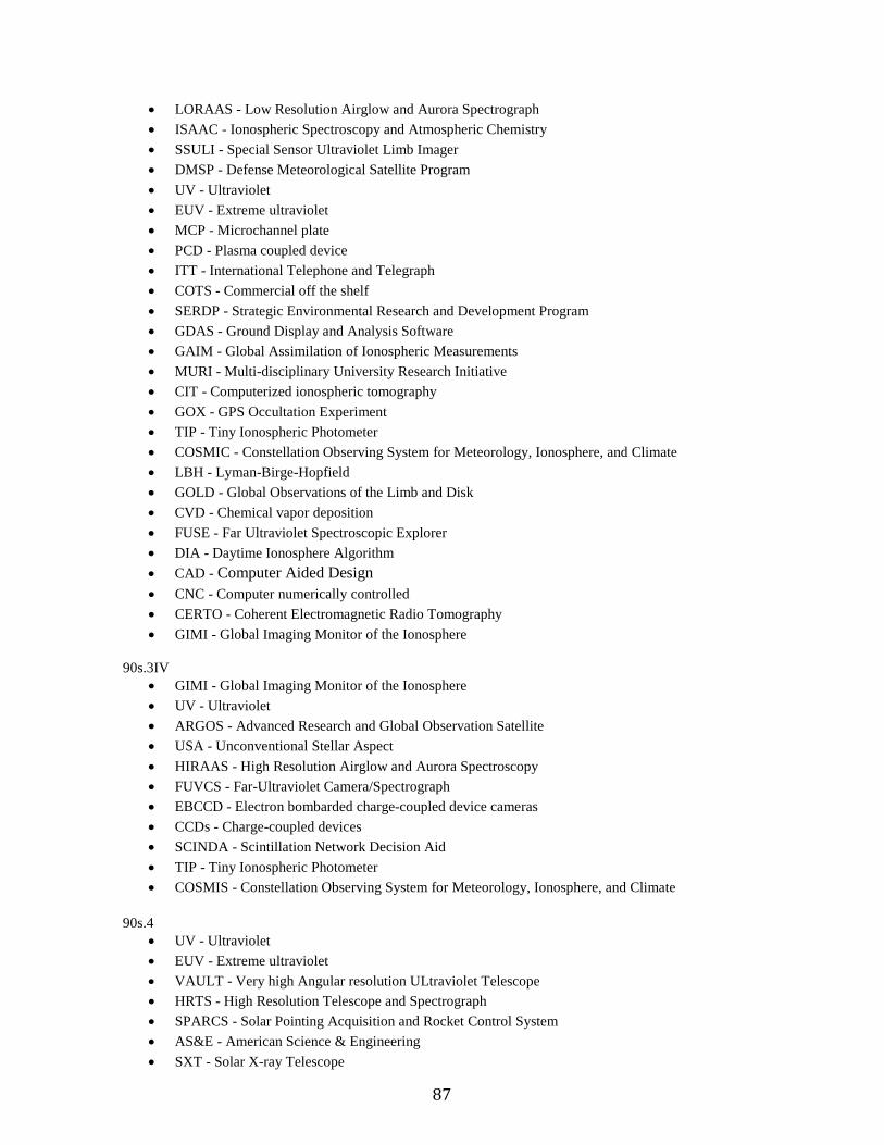
87

• LORAAS - Low Resolution Airglow and Aurora Spectrograph • ISAAC - Ionospheric Spectroscopy and Atmospheric Chemistry • SSULI - Special Sensor Ultraviolet Limb Imager • DMSP - Defense Meteorological Satellite Program • UV - Ultraviolet • EUV - Extreme ultraviolet • MCP - Microchannel plate • PCD - Plasma coupled device • ITT - International Telephone and Telegraph • COTS - Commercial off the shelf • SERDP - Strategic Environmental Research and Development Program • GDAS - Ground Display and Analysis Software • GAIM - Global Assimilation of Ionospheric Measurements • MURI - Multi-disciplinary University Research Initiative • CIT - Computerized ionospheric tomography • GOX - GPS Occultation Experiment • TIP - Tiny Ionospheric Photometer • COSMIC - Constellation Observing System for Meteorology, Ionosphere, and Climate • LBH - Lyman-Birge-Hopfield • GOLD - Global Observations of the Limb and Disk • CVD - Chemical vapor deposition • FUSE - Far Ultraviolet Spectroscopic Explorer • DIA - Daytime Ionosphere Algorithm • CAD - Computer Aided Design • CNC - Computer numerically controlled • CERTO - Coherent Electromagnetic Radio Tomography • GIMI - Global Imaging Monitor of the Ionosphere

90s.3IV • GIMI - Global Imaging Monitor of the Ionosphere • UV - Ultraviolet • ARGOS - Advanced Research and Global Observation Satellite • USA - Unconventional Stellar Aspect • HIRAAS - High Resolution Airglow and Aurora Spectroscopy • FUVCS - Far-Ultraviolet Camera/Spectrograph • EBCCD - Electron bombarded charge-coupled device cameras • CCDs - Charge-coupled devices • SCINDA - Scintillation Network Decision Aid • TIP - Tiny Ionospheric Photometer • COSMIS - Constellation Observing System for Meteorology, Ionosphere, and Climate

90s.4

• UV - Ultraviolet • EUV - Extreme ultraviolet • VAULT - Very high Angular resolution ULtraviolet Telescope • HRTS - High Resolution Telescope and Spectrograph • SPARCS - Solar Pointing Acquisition and Rocket Control System • AS&E - American Science & Engineering • SXT - Solar X-ray Telescope

88

• MDI - Michelson Doppler Imager • EIT - Extreme-ultraviolet Imaging Telescope • CDS - Coronal Diagnostics Explorer imaging spectrometer • SUMER - Solar Ultraviolet Measurements of Emitted Radiation • SOHO - Solar & Heliospheric Observatory • TRACE - Transition Region and Coronal Explorer • WSMR - White Sands Missile Range • STEREO - Solar Terrestrial Relations Observatory

90s.5 • MWFM - Mountain Wave Forecast Model • DoD - Department of Defense • HALE - high-altitude long-endurance • USAF - United States Air Force • UAS - Unmanned Aircraft System • BAMS - Broad Area Maritime Surveillance • CAT - Clear-air turbulence • stratCAT - Stratospheric clear-air turbulence • NWP - Numerical weather prediction • PSCs - Polar stratospheric clouds • SOLVE/THESEO - SAGE III Ozone Loss and Validation Experiment /Third European Stratospheric

Experiment on Ozone 2000 • AFIT - Air Force Institute of Technology • AFWA - Air Force Weather Agency • R&D - Research and development • COAMPS - Coupled Ocean-Atmosphere Mesoscale Prediction System • NAVGEM - Navy Global Environmental Model • ESPC - Earth System Prediction Capabilities

90s.6 • UV - Ultraviolet • G2S - Ground-to-Space • MSISE - Mass Spectrometer & Incoherent Scatter Extended atmospheric model • GFSC - Goddard Space Flight Center • MS - Mass spectrometers • IS - Incoherent scatter • HWM - Horizontal Wind Model • UARS - Upper Atmosphere Research Satellite • NWP - Numerical weather prediction • GEOS - Global Earth Observing System • ECMWF - European Center for Medium Range Weather Forecasting • GFS - Global Forecast System • NOGAPS - Navy Operational Global Atmospheric Prediction System • WAM - Whole Atmospheric Models • ISES - Integrated Sun-Earth System • SSULI - Special Sensor Ultraviolet Limb Imager • GUVI - Global Ultraviolet Imager • COSPAR - Committee on Space Research • CIRA - COSPAR International Reference Atmosphere