voltage control in a distribution system using active

Scholars' Mine Scholars' Mine

Masters Theses Student Theses and Dissertations

Fall 2016

Voltage control in a distribution system using active power loads Voltage control in a distribution system using active power loads

Mounika Chava

Follow this and additional works at: https://scholarsmine.mst.edu/masters_theses

Part of the Electrical and Computer Engineering Commons

Department: Department:

Recommended Citation Recommended Citation Chava, Mounika, "Voltage control in a distribution system using active power loads" (2016). Masters Theses. 7594. https://scholarsmine.mst.edu/masters_theses/7594

This thesis is brought to you by Scholars' Mine, a service of the Missouri S&T Library and Learning Resources. This work is protected by U. S. Copyright Law. Unauthorized use including reproduction for redistribution requires the permission of the copyright holder. For more information, please contact [email protected].

https://library.mst.edu/

https://library.mst.edu/

https://scholarsmine.mst.edu/

https://scholarsmine.mst.edu/masters_theses

https://scholarsmine.mst.edu/student-tds

https://scholarsmine.mst.edu/masters_theses?utm_source=scholarsmine.mst.edu%2Fmasters_theses%2F7594&utm_medium=PDF&utm_campaign=PDFCoverPages

http://network.bepress.com/hgg/discipline/266?utm_source=scholarsmine.mst.edu%2Fmasters_theses%2F7594&utm_medium=PDF&utm_campaign=PDFCoverPages

https://scholarsmine.mst.edu/masters_theses/7594?utm_source=scholarsmine.mst.edu%2Fmasters_theses%2F7594&utm_medium=PDF&utm_campaign=PDFCoverPages

mailto:[email protected]

VOLTAGE CONTROL IN A DISTRIBUTION SYSTEM USING ACTIVE POWER

LOADS

by

MOUNIKA CHAVA

A THESIS

Presented to the Faculty of the Graduate School of the

MISSOURI UNIVERSITY OF SCIENCE AND TECHNOLOGY

In Partial Fulfillment of the Requirements for the Degree

MASTER OF SCIENCE IN ELECTRICAL ENGINEERING

2016

Approved by

Jhi-Young Joo, Advisor

Mariesa L. Crow

Pourya Shamsi

©2016

Mounika Chava

All rights reserved

iii

ABSTRACT

High penetration of renewable energy resources such as rooftop solar photovoltaic

(PV) systems is exacerbating violations of the voltage limits in power distribution

networks. Existing solutions to these over-/under-voltage issues include tap-changing

transformers and shunt capacitors. However, tap changers only allow voltage changes in

discrete steps and shunt capacitors cannot handle over-voltage situations. To overcome

these problems, this thesis proposes voltage control in a distribution system by adjusting

active power loads. The proposed solution can be used for both under- and over-voltage

cases at any levels of voltage adjustment. First, the active power that needs to be adjusted

at selected nodes to bring the voltages within acceptable limits is calculated for under and

over-voltage cases using alternating current optimal power flow (ACOPF). ACOPF is

solved for three different cases by varying the cost of active power adjustment and the

marginal cost from the feeder supply, which is assumed to be the market price. Secondly,

demand response on electric water heaters is implemented to achieve active power

adjustments at selected nodes obtained from the ACOPF results. The problem is

formulated over multiple time steps to minimize the energy costs of water heaters at a

specific node subject to the dynamics of the water temperature, the energy consumption,

the temperature constraints, and the voltage limits at the node. The IEEE 34-bus radial

distribution system is used as a case study. By solving the same problem for different

price settings, it is observed that the price structure affects the energy demand only in the

under-voltage system, but not in the over-voltage system. The main contribution of this

thesis is to show that by adjusting active power loads, voltages in a distribution system

can be maintained within the permissible limits.

iv

ACKNOWLEDGMENTS

First, I would like to thank my advisor, Dr. Jhi Young Joo, for giving me the

opportunity to work on this thesis. She has been a great support throughout my Master’s

program. I am grateful for the guidance she provided and for her valuable time.

Second, I would also like to thank my thesis committee members, Dr. Mariesa L.

Crow and Dr. Pourya Shamsi, for their guidance and taking time to review my thesis

work.

I would like to thank my lab mate, Maigha, for her timely help.

Finally, I would like to thank my parents for their love and support, who stood by

me and supported all my decisions.

v

TABLE OF CONTENTS

Page

ABSTRACT ....................................................................................................................... iii

ACKNOWLEDGMENTS ................................................................................................. iv

LIST OF FIGURES ........................................................................................................... vi

LIST OF TABLES ........................................................................................................... viii

SECTION

1. INTRODUCTION .............................................................................................. 1

1.1 BACKGROUND ................................................................................................ 1

1.2 PROBLEM STATEMENT ................................................................................ 2

2. FORMULATION AND METHODOLOGY ..................................................... 4

2.1 ACOPF FORMULATION ................................................................................. 4

2.2 DEMAND RESPONSE PROBLEM FORMULATION ................................... 5

2.2.1 Electric Water Heater Mode .................................................................... 5

2.2.2 DR Problem Formulation ......................................................................... 7

3. SIMULATION RESULTS ............................................................................... 10

3.1 ACTIVE POWER ADJUSTMENT ................................................................. 10

3.1.1 Under-voltage System ............................................................................ 12

3.1.2. Over-voltage System .............................................................................. 16

3.2 DEMAND RESPONSE MODEL .................................................................... 21

3.2.1 Under-voltage System.. .......................................................................... 22

3.2.2 Over-voltage System. ............................................................................. 30

4. CONCLUSION ................................................................................................ 36

BIBLIOGRAPHY ............................................................................................................. 37

VITA …………………………………………………………………………………….40

vi

LIST OF FIGURES

Page

Figure 2.1. Block diagram of water heater model .............................................................. 6

Figure 3.1. IEEE 34 bus system ........................................................................................ 10

Figure 3.2. Voltage profile of initial, under-voltage and over-voltage test system .......... 11

Figure 3.3. Under-voltage test system .............................................................................. 13

Figure 3.4. Voltage Profile of under-voltage test system ................................................. 15

Figure 3.5. Over-voltage test system ................................................................................ 17

Figure 3.6. Voltage Profile of over-voltage test system ................................................... 20

Figure 3.7. Electricity price settings 1, 2 and 3 ................................................................ 23

Figure 3.8. Hot water usage profiles of houses 1, 2 and 3 at node 824 ............................ 24

Figure 3.9. Energy consumption at node 824 a) price setting 1

b) price settings 2 and 3 ................................................................................. 25

Figure 3.10. Temperature profile at node 824 a) house 1 b) house 2 ............................... 25

Figure 3.11. Temperature profile of house 3 at node 824 ................................................. 26

Figure 3.12. Hot water usage profiles of house 1 and 2 at node 834 ................................ 26


b) price settings 2 and 3 ................................................................................ 27


Figure 3.15. Hot water usage profiles of houses 1 and 2 at node 836 .............................. 28




Figure 3.18. Hot water usage profiles 1, 2 and 3 ............................................................ 31


b) price setting 2 and 3 ................................................................................. 32

Figure 3.20. Temperature profiles at node 824 a) house 1 b) house 2 .............................. 32

Figure 3.21. Temperature profile of house 3 at node 824 ................................................. 33




vii


b) price setting 2 and 3 ................................................................................. 34


viii

LIST OF TABLES

Page

Table 3.1. Total load of the system ................................................................................... 11

Table 3.2. Active and Reactive power limits for under and over-voltage system ............ 12

Table 3.3. ACOPF with adjusting active power only at the slack bus.............................. 13

Table 3.4. ACOPF with slack bus and active power adjustment for Cases 1, 2 and 3 ..... 14

Table 3.5. Cost analysis of correcting voltages in the under-voltage system ................... 16

Table 3.6. Active power adjustment at feeder and selected nodes ................................... 17

Table 3.7. Comparison between cost for feeder adjustment and cost for adjustment at

nodes 824, 834 and 836 for 3 cases ................................................................. 18

Table 3.8. ACOPF with only slack bus generation ........................................................... 19

Table 3.9. ACOPF with slack bus and active power adjustment for cases 1, 2 and 3 ...... 19

Table 3.10. Cost analysis of correcting voltages in the over-voltage system ................... 21

Table 3.11. Active power adjustments in under & over-voltage system .......................... 21

Table 3.12. Simulation parameter setup ........................................................................... 22

Table 3.13. Maximum energy consumption limit for under-voltage system .................... 23

Table 3.14. Minimum energy consumption limits for over-voltage system ..................... 30

1. INTRODUCTION

1.1 BACKGROUND

In power systems, the voltage at each node is maintained between above and

below 5% of the rated value. An electric power distribution system is generally designed

as a radial system, which is arranged in a tree like structure with usually only one power

supply source at the beginning of the feeder. Due to this structure, distribution systems

are more prone to voltage issues than the transmission system.

Under-voltages may be the result of 1) faults on the power system 2) capacitor

bank switching off 3) high load on the system 4) loss of renewable distributed generation.

Over voltages can occur because of 1) switching off high load 2) energizing a capacitor

bank [2] 3) high penetration of distributed generation renewable sources particularly solar

[3].

The voltage issues in a distribution system have become worse with increase in

uncontrollable renewable distributed generation especially solar photovoltaic (PV). In the

last few years, there has been a dramatic increase in renewable distributed generation.

With the increasing PV, high PV penetration and low demand together can lead to over-

voltage problems [18]. On the other hand, when there is peak load and low PV

generation, voltage can drop below lower limit causing under-voltage issues [12].

There have been various studies on mitigating voltage violation problems in

distribution system considering DG renewable energy resources. Reference [24] presents

impact of distributed generation on voltages especially voltage sag problems. Reference

[26] addressed effect of PV power variability on voltage regulation in distribution system

considering 20% of PV penetration. The typical approach is to provide reactive power

support from inverter units to tackle the voltage rise caused by high penetration of PV

[8], [9], [10], [11] and [21]. References [19] and [21] proposed PV generation curtailment

to prevent over voltages. Reference [20] suggested use of shunt reactors, shunt capacitors

and transformer tap changer to prevent voltage instability. However, the tap changers

only allow voltage change at discrete steps. Reactive power is adjusted at the point of PV

installation to mitigate voltage rise problems [23]. The authors of [25] suggested use of

onsite battery energy storage that is integrated with PV inverter to reduce the effects of

2

PV output variability. Reference [27] proposed use of PV over production in the LV

feeder by shifting the peak loads i.e. demand side management and compared it against

the PV energy curtailment.

In this thesis, maintaining the bus voltages (under-voltages and over-voltages)

within the acceptable limits is achieved using demand response (DR) with active power

loads. The proposed solution can be used for both under and over-voltage issues and any

level of voltage adjustment can be achieved.

Demand response is defined as “changes in electric usage by end use customers from

their normal consumption patterns in response to changes in the price of electricity over

time or incentive payments” [5]. In this thesis, electric water heaters are used as

controllable loads for demand response (DR). Water heaters contribute a large portion of

household loads in the U.S. and have following advantages to implement demand

response [6]

Water heaters have relatively high consumption, which is up to 30% of household

load compared to other home appliances [6]

The heating element in an electric water heater is a resistor, which does not

require reactive power support. Main aim is to adjust only active power but not

reactive power

1.2 PROBLEM STATEMENT

This section describes the objective of the thesis problem and steps involved in it.

The main goal is to control the voltage in a distribution system by adjusting active power

loads. The first step is to determine the active power adjustments needed to bring the

voltages within limits. Over-voltage and under-voltage cases were setup by increasing

and decreasing the system load respectively. These under-voltage and over-voltage

systems are used for the rest of study and analysis. Few nodes has been selected to adjust

the active power and assumed that the active power at those nodes can be adjusted.

ACOPF problem (as shown in Section 2) is then formulated by modeling the load buses

where the active power can be adjusted as generation buses. The ACOPF problem is

modeled and solved over one time step in MATPOWER. The ACOPF results provide

3

information on the optimal feeder source generation and active power adjustment needed

at the selected nodes to maintain voltages within acceptable limits.

The second step is to achieve the active power adjustments at selected nodes

obtained in step one using demand response on electric water heaters. A demand response

model for electric water heaters is designed (as given in Section 2) over multiple time

steps minimizing the energy costs subject to the dynamics of the water temperature,

energy and the temperature limits. The DR model is solved over multiple time steps since

the electric water heater cannot be on/off throughout the time and the water temperature

has to be maintained within the temperature limits. The limits on energy consumption are

derived from the active power adjustments obtained in the first step. DR model is

formulated as a mixed integer linear programming and solved in MATLAB.

4

2. FORMULATION AND METHODOLOGY

In this section, first ACOPF problem is formulated that determines the active power

adjustments needed to bring the voltages within permissible limits. Next, a demand

response model on electric water heaters is formulated to achieve the active power

adjustments obtained from the ACOPF solution.

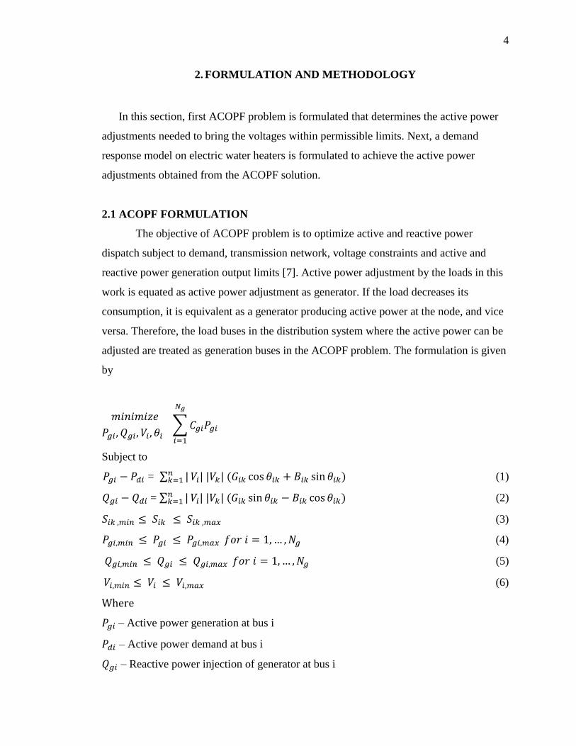
2.1 ACOPF FORMULATION

The objective of ACOPF problem is to optimize active and reactive power

dispatch subject to demand, transmission network, voltage constraints and active and

reactive power generation output limits [7]. Active power adjustment by the loads in this

work is equated as active power adjustment as generator. If the load decreases its

consumption, it is equivalent as a generator producing active power at the node, and vice

versa. Therefore, the load buses in the distribution system where the active power can be

adjusted are treated as generation buses in the ACOPF problem. The formulation is given

by

𝑚𝑖𝑛𝑖𝑚𝑖𝑧𝑒

𝑃𝑔𝑖, 𝑄𝑔𝑖, 𝑉𝑖, 𝜃𝑖 ∑ 𝐶𝑔𝑖𝑃𝑔𝑖

𝑁𝑔

𝑖=1

Subject to

𝑃𝑔𝑖 − 𝑃𝑑𝑖 = ∑ |𝑛𝑘=1 𝑉𝑖| |𝑉𝑘| (𝐺𝑖𝑘 cos 𝜃𝑖𝑘 + 𝐵𝑖𝑘 sin 𝜃𝑖𝑘) (1)

𝑄𝑔𝑖 − 𝑄𝑑𝑖 = ∑ |𝑛𝑘=1 𝑉𝑖| |𝑉𝑘| (𝐺𝑖𝑘 sin 𝜃𝑖𝑘 − 𝐵𝑖𝑘 cos 𝜃𝑖𝑘) (2)

𝑆𝑖𝑘 ,𝑚𝑖𝑛 ≤ 𝑆𝑖𝑘 ≤ 𝑆𝑖𝑘 ,𝑚𝑎𝑥 (3)

𝑃𝑔𝑖,𝑚𝑖𝑛 ≤ 𝑃𝑔𝑖 ≤ 𝑃𝑔𝑖,𝑚𝑎𝑥 𝑓𝑜𝑟 𝑖 = 1, … , 𝑁𝑔 (4)

𝑄𝑔𝑖,𝑚𝑖𝑛 ≤ 𝑄𝑔𝑖 ≤ 𝑄𝑔𝑖,𝑚𝑎𝑥 𝑓𝑜𝑟 𝑖 = 1, … , 𝑁𝑔 (5)

𝑉𝑖,𝑚𝑖𝑛 ≤ 𝑉𝑖 ≤ 𝑉𝑖,𝑚𝑎𝑥 (6)

Where

𝑃𝑔𝑖 – Active power generation at bus i

𝑃𝑑𝑖 – Active power demand at bus i

𝑄𝑔𝑖 – Reactive power injection of generator at bus i

5

𝑄𝑑𝑖 – Reactive power demand at bus i

𝑆𝑖𝑘 - MVA flow on line ik

𝑉𝑖 – Voltage magnitude at bus i

𝐶𝑔𝑖 – Cost function of generator at bus i

𝐺𝑖𝑘 – Conductance of line ik

𝐵𝑖𝑘 – Susceptance of line ik

𝑆𝑖𝑘 ,𝑚𝑖𝑛 , 𝑆𝑖𝑘 ,𝑚𝑎𝑥 – Lower and upper MVA flow limits on line ik

𝑃𝑔𝑖,𝑚𝑖𝑛 , 𝑃𝑔𝑖,𝑚𝑎𝑥 - Lower and upper active power generation limits on line ik

𝑄𝑔𝑖,𝑚𝑖𝑛 , 𝑄𝑔𝑖,𝑚𝑎𝑥 - Lower and upper reactive power generation limits on line ik

𝑉𝑖,𝑚𝑖𝑛 , 𝑉𝑖,𝑚𝑎𝑥 – Lower and upper limit of voltage magnitude at bus i

Equations (1) and (2) are the power flow equations. (3) is related with the lower

and upper flow on the lines. Equation 4 and 5 define active and reactive power limits of

each generating unit. Equation 6 limits voltage at each bus. 𝑃𝑔𝑖 limits for the load buses

are obtained from the original 𝑃𝑑𝑖 at those nodes. ACOPF problem is modeled and solved

in MATPOWER.

2.2 DEMAND RESPONSE PROBLEM FORMULATION

To develop the demand response model, the electric water heater load model is

first derived. Then an optimization problem is formulated for controlling water heaters

with the water temperature dynamics as a constraint.

2.2.1 Electric Water Heater Model. This section presents electric water heater

load model. Figure 2.1 shows the block diagram of the water heater model [14]. The

water heater model parameters are classified into three parts:

1. The temperature profile that includes the ambient temperature, the inlet water

temperature and the hot water temperature set points

2. The water heater characteristics including the heat resistance of the tank (R), the

surface area of the tank (𝑆𝐴𝑡𝑎𝑛𝑘) and the rated power

3. Hot water usage profile by the user

6

Figure 2.1. Block diagram of water heater model

The water temperature in the tank is calculated as [14]

𝑇𝑡+1 =𝑇𝑡(𝑉𝑡𝑎𝑛𝑘 − 𝑉𝑤𝑑. 𝛥𝑡)

𝑉𝑡𝑎𝑛𝑘+

𝑇𝑖𝑛. 𝑉𝑤𝑑. 𝛥𝑡

𝑉𝑡𝑎𝑛𝑘

+1𝑔𝑎𝑙

8.34𝑙𝑏. [𝑃𝑡 . 𝜂.

3412 𝐵𝑡𝑢

𝑘𝑊ℎ−

𝑆𝐴𝑡𝑎𝑛𝑘 . (𝑇𝑡 − 𝑇𝑎𝑚𝑏)

𝑅] .

𝛥𝑡

60𝑚𝑖𝑛

ℎ

.1


(7)

7

where

Tt Water temperature in the tank (℉) in time slot t

Vtank Volume of tank (gallons)

Vwd Volume of hot water withdrawn (gallons per minute)

Δt Duration of each time slot (minutes)

Tin Inlet water temperature (℉)

Pt Electricity demand of water heating unit in time slot t (KW)

SAtank Surface area of the tank (𝑓𝑡2)

Tamb Ambient temperature (℉)

R Heat resistance of tank (℉. 𝑓𝑡2. h/Btu)

𝜂 Efficiency factor

2.2.2 DR Problem Formulation. The objective of demand response model is to

minimize the total energy consumption subject to temperature dynamics of electric water

heater, set point temperature and energy limits. As water temperature has to be

maintained within bounds, the water heater cannot be on or off for the whole hour, hence

the demand response problem has been solved for each 5-minute interval over an hour. It

can be formulated as

𝑚𝑖𝑛𝑖𝑚𝑖𝑧𝑒 ∑ ∑ 𝐶𝑡𝐸𝑡

12

𝑡=1

𝑛

𝑖=1

Subject to

𝑇𝑡+1 =𝑇𝑡(𝑉𝑡𝑎𝑛𝑘 − 𝑉𝑤𝑑. 𝛥𝑡)

𝑉𝑡𝑎𝑛𝑘+

𝑇𝑖𝑛. 𝑉𝑤𝑑. 𝛥𝑡


+1𝑔𝑎𝑙

8.34𝑙𝑏. [𝑃𝑡 . 𝜂.

3412 𝐵𝑡𝑢

𝑘𝑊ℎ−

𝑆𝐴𝑡𝑎𝑛𝑘 . (𝑇𝑡 − 𝑇𝑎𝑚𝑏)

𝑅] .

𝛥𝑡

60𝑚𝑖𝑛

ℎ

.1


(8)

𝑇𝑡,𝑚𝑖𝑛 ≤ 𝑇𝑡 ≤ 𝑇𝑡,𝑚𝑎𝑥 ∀𝑡 (9)

8

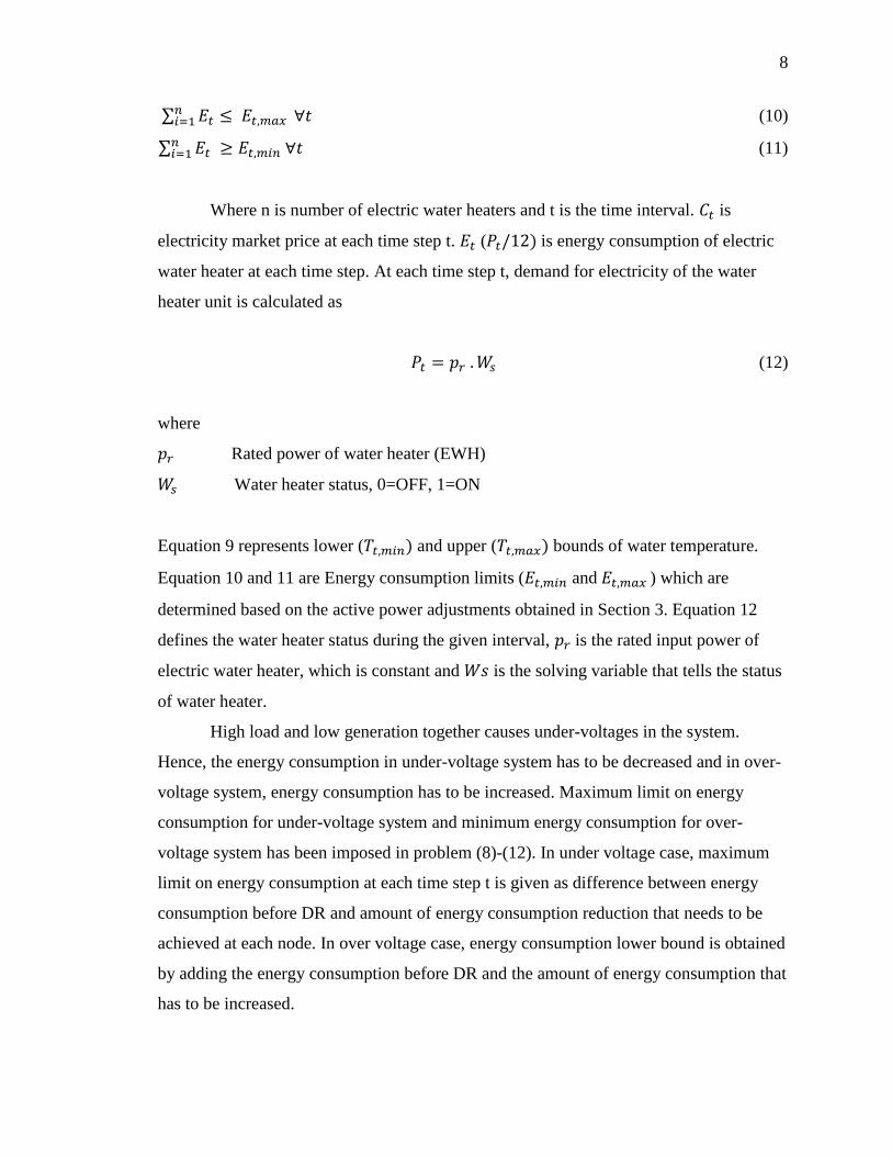
∑ 𝐸𝑡𝑛𝑖=1 ≤ 𝐸𝑡,𝑚𝑎𝑥 ∀𝑡 (10)

∑ 𝐸𝑡𝑛𝑖=1 ≥ 𝐸𝑡,𝑚𝑖𝑛 ∀𝑡 (11)

Where n is number of electric water heaters and t is the time interval. 𝐶𝑡 is

electricity market price at each time step t. 𝐸𝑡 (𝑃𝑡/12) is energy consumption of electric

water heater at each time step. At each time step t, demand for electricity of the water

heater unit is calculated as

𝑃𝑡 = 𝑝𝑟 . 𝑊𝑠 (12)

where

𝑝𝑟 Rated power of water heater (EWH)

𝑊𝑠 Water heater status, 0=OFF, 1=ON

Equation 9 represents lower (𝑇𝑡,𝑚𝑖𝑛) and upper (𝑇𝑡,𝑚𝑎𝑥) bounds of water temperature.

Equation 10 and 11 are Energy consumption limits (𝐸𝑡,𝑚𝑖𝑛 and 𝐸𝑡,𝑚𝑎𝑥 ) which are

determined based on the active power adjustments obtained in Section 3. Equation 12

defines the water heater status during the given interval, 𝑝𝑟 is the rated input power of

electric water heater, which is constant and 𝑊𝑠 is the solving variable that tells the status

of water heater.

High load and low generation together causes under-voltages in the system.

Hence, the energy consumption in under-voltage system has to be decreased and in over-

voltage system, energy consumption has to be increased. Maximum limit on energy

consumption for under-voltage system and minimum energy consumption for over-

voltage system has been imposed in problem (8)-(12). In under voltage case, maximum

limit on energy consumption at each time step t is given as difference between energy

consumption before DR and amount of energy consumption reduction that needs to be

achieved at each node. In over voltage case, energy consumption lower bound is obtained

by adding the energy consumption before DR and the amount of energy consumption that

has to be increased.

9

For the DR optimization problem, expected hot water usage for each house and

the electricity market price are given in 5-minute time intervals, with the initial water

temperature known. The optimization problem is solved using a mixed integer linear

programming with an equality constraint and minimum and maximum bounds. Energy

consumption and water temperature at each time step t are the results of the optimization

problem. To observe the price sensitivity of the loads, the same optimization problem is

solved for different price settings.

10

3. SIMULATION RESULTS

3.1 ACTIVE POWER ADJUSTMENT

The IEEE 34-node radial distribution network with generation at node 800 (slack

bus) is used for the study as shown in Figure 3.1[13]. The test system is modeled after an

actual feeder located in Arizona. The feeder’s nominal voltage is 24.9 kV [13]. The

single-phase balanced test system was modeled in MATPOWER ignoring voltage

regulators between 814 and 850 and between 852 and 832 nodes.

Figure 3.1. IEEE 34 bus system

To study the test system further, the total load was adjusted (as shown in Table

3.1) randomly to setup a system with over voltages and under voltages. Over-voltage and

under-voltage cases were derived by decreasing 13% of the load at each node and by

increasing 16% of the load at each bus respectively.

11

Table 3.1. Total load of the system

Initial system load Under -voltage system load Over-voltage system load

P (MW) Q (Mvar) P (MW) Q (Mvar) P (MW) Q (Mvar)

3.062 1.898 3.55 2.2 2.66 1.65

Figure 3.2 shows the voltage profile of the initial, under-voltage and over-voltage

test system. From the graph, the voltage profile of the initial test system is within limits

(0.95 p.u.-1.05 p.u.). In the under-voltage system, voltages at a few (16) nodes especially

the nodes that are far from the source are below the lower limit (0.95 p.u.). In the over-

voltage system, some of the node voltages are above (1.05 p.u.). After setting up the

under-voltage and over voltage systems, next how much active power needs to be

adjusted is determined to bring the voltages within acceptable limits of 0.95 p.u. to 1.05

p.u. The nodes that have lateral branches (nodes 824, 834, and 836) has been selected and

assumed the active power at those nodes can be adjusted.

Figure 3.2. Voltage profile of initial, under-voltage and over-voltage test system

0.8

0.85

0.9

0.95

1

1.05

1.1

800 806 812 810 816 826 820 828 854 852 858 834 844 848 836 838 888

V

o

l

t

a

g

e

(

P

U)

Node

Initial System Under- voltage system Over-voltage system

12

The ACOPF problem is solved for both under-voltage and over-voltage test

systems, to calculate the active power adjustment to bring the voltages within limits. The

problem is formulated in Section 2. Active power adjustment at nodes 824, 834 and 836

nodes is modeled as generation for solving ACOPF. The solution of the ACOPF problem

gives the optimal slack bus generation and the active power that needs to be adjusted at

nodes 824, 834 and 836.

Maximum active power output limits for the active power adjustment at nodes

824, 834 and 836 is given as 10% of the load at those buses respectively (as shown in

Table 3.2). Reactive power limits are given as zero since the objective is to adjust active

power only.

Table 3.2. Active and Reactive power limits for under and over-voltage system

Under-voltage system Over-voltage system

Bus

Active

Power

(MW)

Reactive

Power

(Mvar)

Active

Power

(MW)

Reactive

Power

(Mvar)

800 100 0 5 −5 100 0 5 −5

824 0.0026 0 0 0 0 −0.0019 0 0

834 0.0020 0 0 0 0 −0.0015 0 0

836 0.0018 0 0 0 0 −0.0013 0 0

3.1.1 Under-voltage System. Figure 3.3 represents the under-voltage test system

and highlighted nodes represent the nodes whose voltages were below 0.95 p.u.

13

Figure 3.3. Under-voltage test system

ACOPF problem is solved for the under-voltage system having only feeder

supply, to obtain the optimal “generation”, or net active power production satisfying the

voltage limits at each node. ACOPF results with adjusting active power only at the slack

bus is given in the Table 3.3.

Table 3.3. ACOPF with adjusting active power only at the slack bus

Bus Slack bus Generation

Active power (MW) Reactive power (Mvar)

800 4.7482 2.8016

ACOPF problem is solved for the under-voltage system for below cases, to

evaluate the economy of adjusting active power at the nodes (i.e., demand response),

compared with the cost of adjusting active power from the feeder supply.

Case 1: Cost of feeder supply ($10/MWh) < cost of active power adjustment ($50/MWh)

Case 2: Cost of feeder supply ($50/MWh) > cost of active power adjustment ($10/MWh)

Case 3: Cost of feeder supply ($10/MWh) = cost of active power adjustment ($10/MWh)

14

Table 3.4 shows the ACOPF results for all three cases. From the results, it is clear

that in Case 1, slack bus is generating the total active and reactive power required by the

system while the active power adjustment at nodes 824, 834 and 836 nodes is zero. This

is because the cost for adjusting active power is higher than the cost of the slack bus

generation.

Table 3.4. ACOPF with slack bus and active power adjustment for Cases 1, 2 and 3

Under voltage test system

Bus

Case 1

cost of

(feeder supply <

adjusting P)

Case 2

cost of

(feeder supply >

adjusting P)

Case 3

cost of

(feeder supply =

adjusting P)

Active

power

(MW)

Reactive

Power

(Mvar)

Active power

(MW)

Reactive

Power

(Mvar)

Active power

(MW)

Reactive

Power

(Mvar)

800 4.7477 2.8016 4.7390 2.8016 4.7391 2.8016

824 0 0 0.0025 0 0.0025 0

834 0 0 0.0020 0 0.0020 0

836 0 0 0.0018 0 0.0018 0

In Case 2, active power adjustment at nodes 824, 834, and 836 is using almost its

full capacity (2,500 W at 824, 2,000 W at 834, and 1,800 W at 836). In total, 6,628 W

needs to be adjusted to bring the voltage profile within the limits.

Case 3 is similar to case 2 where active power adjustment needed at 824, 834 and

836 is its maximum active power limit (2500 W at 824, 2000 W at 834 and 1800 W at

836). To maintain voltage conditions in the under-voltage system, it requires 6,578 W

active power adjustments at nodes 824, 834, and 836.

15

In all three cases, reactive power supplied by the slack (2.801 Mvar) is same. In

Cases 2 and 3 active power adjustment needed is its maximum active power limit where

as in Case 1 it is zero. This is because the cost for active power adjustment is less than or

equal to slack bus generation in Cases 2 and 3.

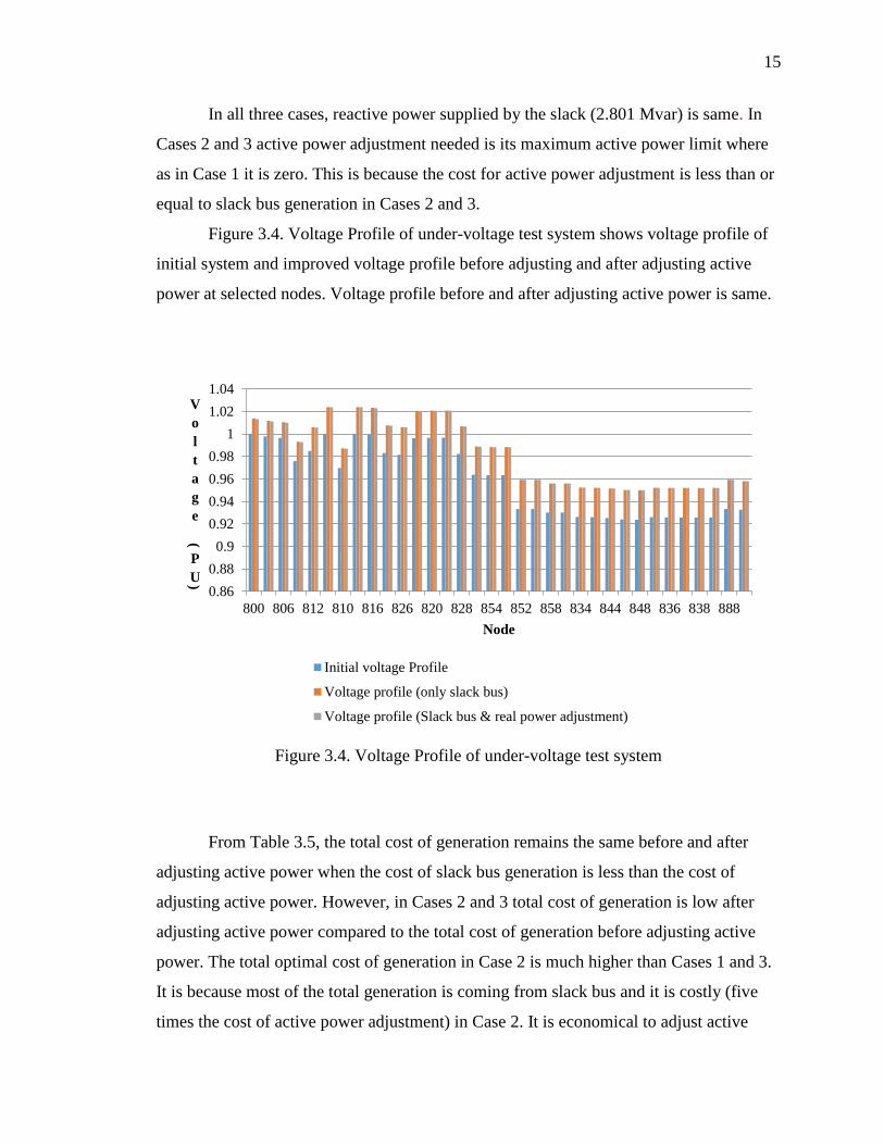
Figure 3.4. Voltage Profile of under-voltage test system shows voltage profile of

initial system and improved voltage profile before adjusting and after adjusting active

power at selected nodes. Voltage profile before and after adjusting active power is same.

Figure 3.4. Voltage Profile of under-voltage test system

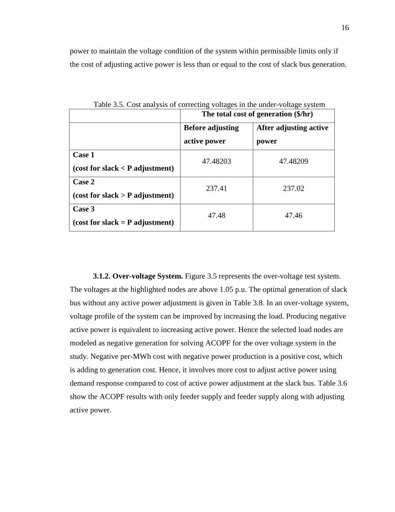
From Table 3.5, the total cost of generation remains the same before and after

adjusting active power when the cost of slack bus generation is less than the cost of

adjusting active power. However, in Cases 2 and 3 total cost of generation is low after

adjusting active power compared to the total cost of generation before adjusting active

power. The total optimal cost of generation in Case 2 is much higher than Cases 1 and 3.

It is because most of the total generation is coming from slack bus and it is costly (five

times the cost of active power adjustment) in Case 2. It is economical to adjust active

0.86

0.88

0.9

0.92

0.94

0.96

0.98

1

1.02

1.04

800 806 812 810 816 826 820 828 854 852 858 834 844 848 836 838 888

V

o

l

t

a

g

e

(

P

U)

Node

Initial voltage Profile

Voltage profile (only slack bus)

Voltage profile (Slack bus & real power adjustment)

16

power to maintain the voltage condition of the system within permissible limits only if

the cost of adjusting active power is less than or equal to the cost of slack bus generation.

Table 3.5. Cost analysis of correcting voltages in the under-voltage system

The total cost of generation ($/hr)

Before adjusting

active power

After adjusting active

power

Case 1

(cost for slack < P adjustment) 47.48203 47.48209

Case 2

(cost for slack > P adjustment) 237.41 237.02

Case 3

(cost for slack = P adjustment) 47.48 47.46

3.1.2. Over-voltage System. Figure 3.5 represents the over-voltage test system.

The voltages at the highlighted nodes are above 1.05 p.u. The optimal generation of slack

bus without any active power adjustment is given in Table 3.8. In an over-voltage system,

voltage profile of the system can be improved by increasing the load. Producing negative

active power is equivalent to increasing active power. Hence the selected load nodes are

modeled as negative generation for solving ACOPF for the over voltage system in the

study. Negative per-MWh cost with negative power production is a positive cost, which

is adding to generation cost. Hence, it involves more cost to adjust active power using

demand response compared to cost of active power adjustment at the slack bus. Table 3.6

show the ACOPF results with only feeder supply and feeder supply along with adjusting

active power.

17

Figure 3.5. Over-voltage test system

Table 3.6. Active power adjustment at feeder and selected nodes

Node Only feeder adjustment

(MW)

Adjustment at slack and nodes

(MW)

800 3.808 3.8142

824 0 −0.0019

834 0 −0.0015

836 0 −0.0013

ACOPF is solved for three different cases

Case 1-

Cost of feeder supply (10 $/MWh) < cost for active power adjustment (-50 $/MWh)

Case 2-

Cost of feeder supply (50 $/MWh) > cost for active power adjustment (-10 $/MWh)

Case 3-

Cost of feeder supply (10 $/MWh) = cost for active power adjustment (-10 $/MWh)

From the Table 3.7, for all the three cases, cost of active power adjustment at the

slack bus is cheaper than the active power adjustment at the nodes 824, 834 and 836.

From simulations, assuming a positive per-Wh cost for active power consumption (or

negative active power production) did not turn out to be an economical option. Therefore,

18

in the over-voltage case, demand response can be economically used only when a

negative cost is assigned to active power consumption (or negative active power

production). In other words, a per-Wh net benefit for active power consumption, which is

equivalent to a negative cost of producing active power is considered. Net benefit of

adjusting active power is defined as revenue minus costs. The costs include maintenance,

losses and costs for implementing demand response, such as meter/controller installation.

Hence, cases 1, 2 and 3 are redefined as

Case 1 –

Cost of feeder supply (10 $/MWh) < net benefit of adjusting active power (50 $/MWh)

Case 2 –

Cost of feeder supply (50 $/MWh) > net benefit of adjusting active power (10 $/MWh)

Case 3 –

Cost of feeder supply (10 $/MWh) = net benefit of adjusting active power (10 $/MWh)

Table 3.7. Comparison between cost for feeder adjustment and cost for adjustment at

nodes 824, 834 and 836 for 3 cases

Cost

for only feeder

adjustment

Cost for

adjustment at

nodes

824,834 and 836

Case 1:

(cost of feeder supply (10 $/MWh) <

cost for active power adjustment (-50 $/MWh) 38.08 38.38

Case 2:

(cost of feeder supply (50 $/MWh) >


Case 3:

(cost of feeder supply (10 $/MWh) =


19

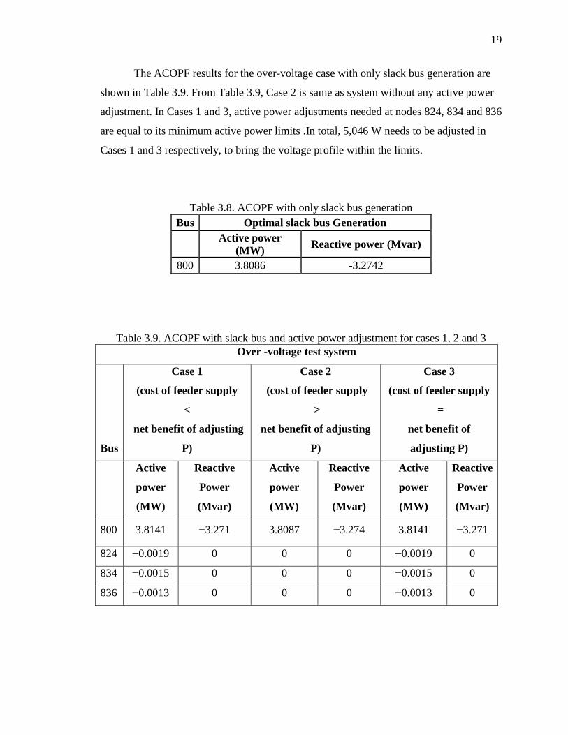
The ACOPF results for the over-voltage case with only slack bus generation are

shown in Table 3.9. From Table 3.9, Case 2 is same as system without any active power

adjustment. In Cases 1 and 3, active power adjustments needed at nodes 824, 834 and 836

are equal to its minimum active power limits .In total, 5,046 W needs to be adjusted in

Cases 1 and 3 respectively, to bring the voltage profile within the limits.

Table 3.8. ACOPF with only slack bus generation

Bus Optimal slack bus Generation

Active power

(MW) Reactive power (Mvar)

800 3.8086 -3.2742

Table 3.9. ACOPF with slack bus and active power adjustment for cases 1, 2 and 3

Over -voltage test system

Bus

Case 1

(cost of feeder supply

<

net benefit of adjusting

P)

Case 2


>

net benefit of adjusting

P)

Case 3


=

net benefit of

adjusting P)

Active

power

(MW)

Reactive

Power

(Mvar)

Active

power

(MW)

Reactive

Power

(Mvar)

Active

power

(MW)

Reactive

Power

(Mvar)

800 3.8141 −3.271 3.8087 −3.274 3.8141 −3.271

824 −0.0019 0 0 0 −0.0019 0

834 −0.0015 0 0 0 −0.0015 0

836 −0.0013 0 0 0 −0.0013 0

20

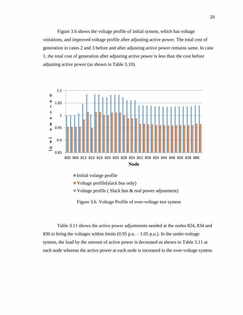
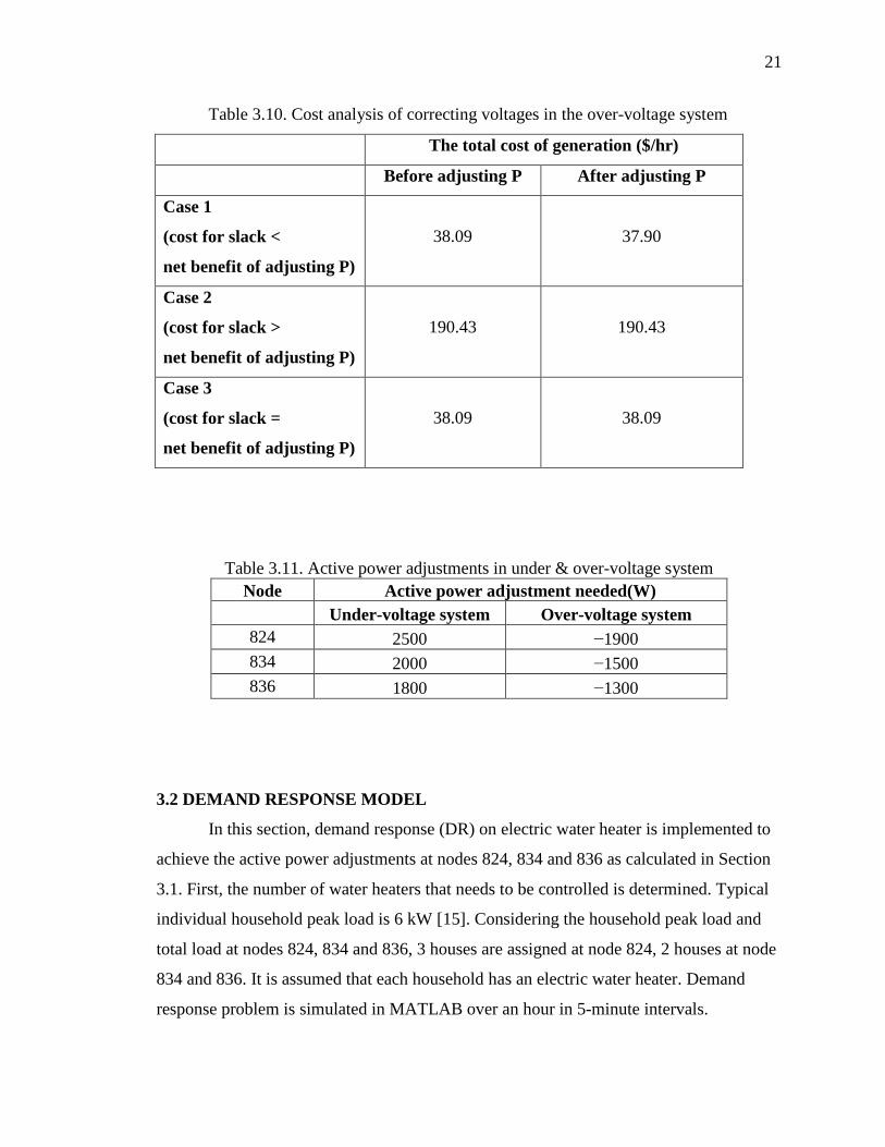
Figure 3.6 shows the voltage profile of initial system, which has voltage

violations, and improved voltage profile after adjusting active power. The total cost of

generation in cases 2 and 3 before and after adjusting active power remains same. In case

1, the total cost of generation after adjusting active power is less than the cost before

adjusting active power (as shown in Table 3.10).

Figure 3.6. Voltage Profile of over-voltage test system

Table 3.11 shows the active power adjustments needed at the nodes 824, 834 and

836 to bring the voltages within limits (0.95 p.u. – 1.05 p.u.). In the under-voltage

system, the load by the amount of active power is decreased as shown in Table 3.11 at

each node whereas the active power at each node is increased in the over-voltage system.

0.85

0.9

0.95

1

1.05

1.1

800 806 812 810 816 826 820 828 854 852 858 834 844 848 836 838 888

V

o

l

t

a

g

e

(

P

U)

Node

Initial volatge profile

Voltage profile(slack bus only)

Voltage profile ( Slack bus & real power adjustment)

21

Table 3.10. Cost analysis of correcting voltages in the over-voltage system

The total cost of generation ($/hr)

Before adjusting P After adjusting P

Case 1

(cost for slack <

net benefit of adjusting P)

38.09 37.90

Case 2

(cost for slack >


190.43 190.43

Case 3

(cost for slack =


38.09 38.09

Table 3.11. Active power adjustments in under & over-voltage system

Node Active power adjustment needed(W)

Under-voltage system Over-voltage system

824 2500 −1900

834 2000 −1500

836 1800 −1300

3.2 DEMAND RESPONSE MODEL

In this section, demand response (DR) on electric water heater is implemented to

achieve the active power adjustments at nodes 824, 834 and 836 as calculated in Section

3.1. First, the number of water heaters that needs to be controlled is determined. Typical

individual household peak load is 6 kW [15]. Considering the household peak load and

total load at nodes 824, 834 and 836, 3 houses are assigned at node 824, 2 houses at node

834 and 836. It is assumed that each household has an electric water heater. Demand

response problem is simulated in MATLAB over an hour in 5-minute intervals.

22

The lower (𝑇𝑡,𝑚𝑖𝑛) and upper (𝑇𝑡,𝑚𝑎𝑥) bounds of the hot water temperature are

considered as 110℉ and 130℉ [17]. Energy consumption limits (𝐸𝑡,𝑚𝑖𝑛 and 𝐸𝑡,𝑚𝑎𝑥 ) is

determined based on the active power adjustments needed at nodes 824, 834 and 836 (as

shown in Table 3.11. Active power adjustments in under & over-voltage system).

Table 3.12 shows the parameters setup [14] needed to run the DR optimization

problem.

Table 3.12. Simulation parameter setup

Attribute Value

Inlet water temperature (𝑇𝑖𝑛) 60 (℉)

Ambient temperature (𝑇𝑎𝑚𝑏) 60 (℉)

Tank volume ( 𝑉𝑡𝑎𝑛𝑘) 40 (gallons)

Heat resistance of tank (R) 20 (℉. 𝑓𝑡2. h/Btu)

Surface area of tank (𝑆𝐴𝑡𝑎𝑛𝑘) 30.8 (𝑓𝑡2)

Rated power (P) 4.5 KW

In order to obtain the price sensitivity of the electric water heater load, the same

optimization problem is solved for three different electricity price profiles (as shown in

Figure 3.7 [16].

3.2.1 Under-voltage System. It is assumed that all the houses at nodes at 824,

834 and 836 are at their peak during the hour. Each house at a node has different water

usage profiles and the initial water temperature is assumed 118℉. Three different water

usage profiles are used for the analysis and are given as Figure 3.8.

First the default case is simulated i.e., before DR when there are no constraints on

the energy consumption of water heaters. The water heater status is determined according

to the following rules: the water heater status is OFF when the tank water temperature is

within the limits. If the tank temperature drops below the lower temperature bound, the

heating coils start working at its rated power until it reaches the upper limit.

23

Figure 3.7. Electricity price settings 1, 2 and 3

To solve the DR model (formulated in Section 2), 𝐸𝑡,𝑚𝑎𝑥 has to be determined at

each node as they vary with the active power adjustment needed at each node.

Et,max = consumption before DR −active adjustment needed at the node

12

(13)

Hence, 𝐸𝑡,𝑚𝑎𝑥 at each node is given as in Table 3.13. The inputs to DR model and

simulated results before and after DR at each node are arranged in following order

1. Hot water usage [17]

2. Total energy consumption

3. Water temperature profile of each electric water heater

Table 3.13. Maximum energy consumption limit for under-voltage system

Node 𝐄𝐭,𝐦𝐚𝐱 (kWh)

824 0.911583

834 0.957583

836 0.970833

2.2

2.4

2.6

2.8

3

0 2 4 6 8 10 12

Ele

ctri

city

Pri

ce

(¢/k

Wh

)

Time

Price setting 1

Price setting 2

Price setting 3

24

Figure 3.8. Hot water usage profiles of houses 1, 2 and 3 at node 824

Figures 3.9, 3.10 and 3.11 are the DR results at node 824. From Figure 3.9, total

energy consumption over an hour at node 824 before and after DR is 10.125kWh and

6.375 kWh respectively.

At node 824, as the upper limit on energy consumption is 0.911583kWh, during

any interval, maximum number of water heaters that are allowed to operate is two. From

Figure 3.9, before DR three water heaters are ON during 6th,7th,8th,9th,10th,11th and 12th

intervals but after DR, maximum number of water heaters ON in any of the intervals is

two.

Before DR when water temperature drops below the lower bound (110℉), the

heating element starts working and tries to reach the upper bound (130℉). The demand

response model does not require the water temperature to reach its maximum but it

maintains the temperature between 110℉ and 130℉ minimizing the energy consumption.

From Figure 3.10 and 3.11 before DR, water temperature dropped below 110℉ before

0

0.1

0.2

0.3

0.4

0.5

0.6

0.7

0 2 4 6 8 10 12

Hot

wate

r co

nsu

mp

tion

(gal/

min

)

Time

Hot water consumption (gal/min), house 1

House 1 House 2 House 3

25

and during the fifth interval. From then, the water heater is ON until the last interval to

reach the maximum temperature limit.

Figure 3.9. Energy consumption at node 824 a) price setting 1 b) price settings 2 and 3

Figure 3.10. Temperature profile at node 824 a) house 1 b) house 2

0

0.2

0.4

0.6

0.8

1

1.2

0 5 10

En

erg

y C

on

sum

pti

on

(k

Wh

)

Time

Energy consumption (kWh)

Before DR After DR

0

0.1

0.2

0.3

0.4

0.5

0.6

0.7

0.8

0 5 10

Ener

gy C

onsu

mp

tio

n (

kW

h)

Time


Price setting 2 Price setting 3

106

108

110

112

114

116

118

120

122

0 5 10

Wa

ter T

emp

era

ture

(℉

)

Time

Temperature Profile, House 1

Before DR After DR

108

110

112

114

116

118

120

122

0 5 10

Wa

ter T

emp

era

ture

(℉

)

Time


Before DR After DR

26

Figure 3.11. Temperature profile of house 3 at node 824

By solving the same optimization problem for different price settings, obtained

different energy usage at each time step are obtained. Energy consumption for price

settings 2 and 3 is obtained and shown in Figure 3.9. From Figure 3.9, total energy

consumption is same for all price settings but the energy usage over a particular time

interval is different. Figure 3.12 shows the hot water usage profile of house 1 and 2 at

node 834.

Figure 3.12. Hot water usage profiles of house 1 and 2 at node 834

108

110

112

114

116

118

120

122

0 2 4 6 8 10 12

Wa

ter T

emp

era

ture

(℉

)

Time


Before DR After DR

0

0.2

0.4

0.6

0.8

1

0 2 4 6 8 10 12

Ho

t w

ate

r c

on

sum

pti

on

(g

al/

min

)

Time

Hot water consumption (gal/min)

House 1

House 2

27

By solving the DR model at node 834, obtained results as shown in Figure 3.13

and 3.14. From Figure 3.13, total energy consumption at node 834 for price setting 1

before and after DR is 6.75 kWh and 4.125 kWh respectively.



0

0.2

0.4

0.6

0.8

0 5 10 15En

erg

y c

on

sum

pti

on

(k

Wh

)

Time


Before DR After DR

0

0.1

0.2

0.3

0.4

0 5 10

En

erg

y c

on

sum

pti

on

(k

Wh

)

Time



108

110

112

114

116

118

120

122

0 5 10

Tem

per

atu

re (

℉)

Time

Before DR After DR

106

108

110

112

114

116

118

120

0 5 10

Tem

per

atu

re (

℉)

Time

Before DR After DR

28

Before DR, both the water heaters are ON from 5th interval to 12th interval but

after DR due to limit on energy consumption, any one of the water heaters is allowed to

operate at time step t. From Figure 3.13, it is clear that only one water heater is on while

the other water heaters are off at a given time interval.

Figure 3.14 represents water temperature profile for each house at node 834

before and after DR. From Figure 3.14, before DR water temperature dropped below

110℉ at second and fifth intervals for electric water heater one and two respectively.

From then until the last interval, water heater is ON to bring the water temperature to its

maximum. After DR, the water temperatures are maintained between 110℉ and 130℉.

By solving the same DR model at node 834 for different price settings 2 and 3,

energy consumption of water heater is obtained as shown in Figure 3.13. Total energy

consumption over an hour is same for price setting one, two and three but energy usage in

a specific time interval varies with the price structure. Hot water usage at node 834 is

given as in Figure 3.15.

Figure 3.15. Hot water usage profiles of houses 1 and 2 at node 836

Similar to the results at nodes 824 and 834, energy consumption and temperature

profile of water heaters 1 anad 2 at node 836 is given in Figures 3.16 and 3.17. From

0

0.2

0.4

0.6

0.8

1

0 2 4 6 8 10 12 14

Ho

t w

ate

r u

sag

e (g

al/

min

)

Hot water usage(gal/min)

House 1 House 2

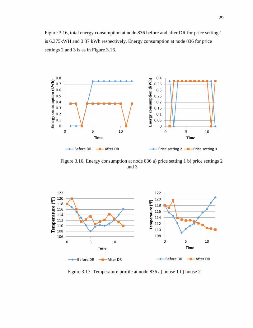
29

Figure 3.16, total energy consumption at node 836 before and after DR for price setting 1

is 6.375kWH and 3.37 kWh respectively. Energy consumption at node 836 for price

settings 2 and 3 is as in Figure 3.16.

Figure 3.16. Energy consumption at node 836 a) price setting 1 b) price settings 2

and 3


0

0.1

0.2

0.3

0.4

0.5

0.6

0.7

0.8

0 5 10

En

erg

y c

on

sum

pti

on

(k

Wh

)

Time

Before DR After DR

0

0.05

0.1

0.15

0.2

0.25

0.3

0.35

0.4

0 5 10

En

erg

y c

on

sum

pti

on

(k

Wh

)

Time


106

108

110

112

114

116

118

120

122

0 5 10 15

Tem

per

atu

re (

℉)

Time

Before DR After DR

108

110

112

114

116

118

120

122

0 5 10

Tem

pe

ratu

re (

℉)

Time

Before DR After DR

30

Total energy consumption remains same for all price settings but the energy usage

over a time step t varies with price structure.

Figure 3.17 represents water temperature profiles water heater 1 and 2. Before

DR, water temperature dropped below 110℉ during 5th and 4th time intervals. From then

the water heaters are on until the the last time interval trying to reach the maximum limit.

After DR, temperatures are maintained between limits (110℉ 130℉ ).

3.2.2 Over-voltage System. Over-voltages are due to high generation or less

load. The load is increased by the amount of active power as calculated in Section 3.1. In

over-voltage case, limits on the minimum energy demand is imposed. The initial

temperature is assumed 115℉. Hence, 𝑬𝒕,𝒎𝒊𝒏 at each node is calculated using below

equation (given as in Table 3.14).

Et,min = consumption before DR +active adjustment needed at the node

12

(14)

Table 3.14. Minimum energy consumption limits for over-voltage system

Node 𝐄𝐭,𝐦𝐢𝐧 (kWh)

824 0.1628

834 0.1265

836 0.11571

The hot water usage demand is very low in the over-voltage system compared to

the demand in the under-voltage system. Three different hot water usage profiles are

defined as shown in Figure 3.18. As the hot water usage is very low, the energy

consumption of water heaters at node 824 before DR is 0 and the water temperature is

between 110℉ and 130℉ during all the intervals. In the DR model as limits on minimum

energy consumption (0.1628 kWh) has been imposed throughout the whole period, this

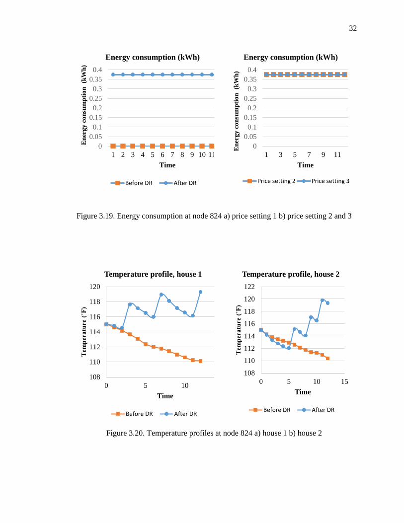
means that any one of the three water heaters has to be on at each interval. Figure 3.19

shows the energy consumption of water heaters at node 824 before and after DR. From

the Figure 3.19, energy consumption before DR is zero because of low water usage. After

31

DR, energy consumption is set to its minimum limit i.e. any one of the three water

heaters are on during any given interval.

Figure 3.18. Hot water usage profiles 1, 2 and 3

The same optimization problem is solved for different price settings to observe

the price sensitivity. Unlike the under-voltage system case, price does not have any effect

on the energy consumption in the over-voltage system. This is because of the constraint

on the minimum energy consumption of water heaters. The result of DR model is setting

energy usage output at the minimum limit (shown in Figure 3.19).

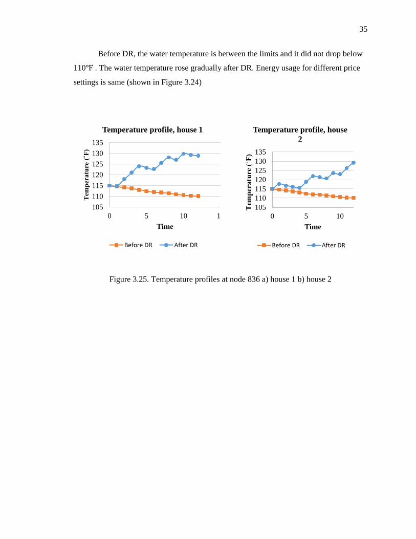
From Figure 3.20 and 3.21 before DR, the water temperature profile during all the

intervals is between 110℉ and 130℉, it did not drop below 110℉ hence water heater

status is off and energy consumption is zero. After DR, since the water heaters, one and

two are on for 15 minutes and water heater 3 is on for 30-minutes.Hnece, water

temperature of each water heater raised gradually compared to the default case.

0

0.02

0.04

0.06

0.08

0.1

0.12

0.14

0 2 4 6 8 10 12

Ho

t w

ate

r c

on

sum

pti

on

(g

al/

min

)

Time

Hot water consumption (gal/min)

Profile 1 Profile 2 Profile 3

32

Figure 3.19. Energy consumption at node 824 a) price setting 1 b) price setting 2 and 3

Figure 3.20. Temperature profiles at node 824 a) house 1 b) house 2

0

0.05

0.1

0.15

0.2

0.25

0.3

0.35

0.4

1 2 3 4 5 6 7 8 9 10 11 12

En

erg

y c

on

sum

pti

on

(k

Wh

)

Time


Before DR After DR

0

0.05

0.1

0.15

0.2

0.25

0.3

0.35

0.4

1 3 5 7 9 11

En

erg

y c

on

sum

pti

on

(k

Wh

)

Time



108

110

112

114

116

118

120

0 5 10 15

Tem

per

atu

re (

˚F)

Time

Temperature profile, house 1

Before DR After DR

108

110

112

114

116

118

120

122

0 5 10 15

Tem

per

atu

re (

˚F)

Time


Before DR After DR

33

Figure 3.21. Temperature profile of house 3 at node 824

Figure 3.22 and 3.24 are the results of DR at node 834. Hot water usage profile 1

and 2, price settings 1 and 2 are given as inputs to DR model. From Figure 3.22, before

DR the energy usage is zero. Since the water temperature did not drop below 110℉,

water heater is off throughout the period. After DR, any one of the waters is on during all

the intervals because of the limit on minimum energy consumption. Hence the water

temperature of water heater 1 and 2 increased gradually (shown in Figure 3.23).


105

110

115

120

125

130

135

0 2 4 6 8 10 12 14

Tem

per

atu

re (

˚F)

Time


Before DR After DR

0

0.1

0.2

0.3

0.4

1 2 3 4 5 6 7 8 9 10 11 12

En

erg

y c

on

sum

pti

on

(k

Wh

)

Time


Before DR After DR

0

0.1

0.2

0.3

0.4

1 3 5 7 9 11

En

erg

y c

on

sum

pti

on

(k

Wh

)

Time



34


Water heater is not required to be on because for the given low water usage, water

temperature is within limits. Since the objective of DR model is to minimize energy costs

satisfying energy and the temperature constraints, it is setting the energy usage at its

minimum limit. The DR results at node 836 are shown in Figure 3.24 and 3.25. Similar to

the energy consumption at node 824 and 834, from Figure 3.24 energy usage at node 836

before DR is 0 and it is at its minimum limit after DR.

Figure 3.24. Energy consumption at node 836 a) price setting 1 b) price setting 2 and 3

105

110

115

120

125

130

135

0 5 10 15

Tem

per

atu

re (

˚F)

Time


Before DR After DR

105

110

115

120

125

130

135

0 5 10

Tem

per

atu

re (

˚F)

Time


Before DR After DR

0

0.1

0.2

0.3

0.4

1 3 5 7 9 11

En

erg

y c

on

sum

pti

on

(k

Wh

)

Time



0

0.1

0.2

0.3

0.4

1 2 3 4 5 6 7 8 9 101112

En

erg

y c

on

sum

pti

on

(k

Wh

)

Time


Before DR After DR

35

Before DR, the water temperature is between the limits and it did not drop below

110℉ . The water temperature rose gradually after DR. Energy usage for different price

settings is same (shown in Figure 3.24)


105

110

115

120

125

130

135

0 5 10 15

Tem

per

atu

re (

˚F)

Time


Before DR After DR

105

110

115

120

125

130

135

0 5 10

Tem

per

atu

re (

˚F)

Time

Temperature profile, house

2

Before DR After DR

36

4. CONCLUSION

This thesis provides an approach to maintain voltages within the limits in a

distribution system with active power adjustment. The ACOPF problem is solved to

calculate the active power adjustments at each node to bring the violated voltages within

the limits. The problem is solved for three different cases where the marginal cost of

feeder supply and the cost of active power adjustment were varied. The solution to this

problem i.e., the active power adjustments at eligible nodes was realized by adjusting

energy consumption of electric water heaters. It can be concluded that voltages in a

distribution system can be maintained within limits by adjusting active power using

demand response. This is especially economical when the cost of adjusting active power

with loads is lower than or equal to the cost form the feeder supply in under-voltage

system. In over-voltage case, demand response is economical when cost of feeder supply

is less than net benefit of adjusting P.

There is much future work ahead where the assumption on nodes that has the

active power adjustment capability that were made to show the proof of concept can be

relaxed and systematic approach can be defined. Assumptions that were made in solving

demand response on electric water heater temperature such as the same initial

temperature, inlet and ambient temperature for all the houses can be relaxed and more

variability can be included.

.

37

BIBLIOGRAPHY

[1] Akash T. Davda, Bhupendra. R. Parekh “System Impact Analysis of Renewable

Distributed Generation on an Existing Radial Distribution Network” 2012 IEEE

Electrical Power and Energy Conference.

[2] Surya Santoso “Fundamentals of Electric Power Quality” 2010.

[3] E. Liu and J. Bebic “Distribution System Voltage Performance Analysis for High-

Penetration Photovoltaics” [online].

https://www1.eere.energy.gov/solar/pdfs/42298.pdf.

[4] W. El-Khattam and M. M. A. Salama, “Distributed Generation technologies,

definitions and benefits” in Electric Power Systems Research., 2004.

[5] W. El-Khattam and M. M. A. Salama, “Benefits of demand response in electricity

markets and recommendations for achieving them” [online]. Available:

http://energy.gov/sites/prod/files/oeprod/DocumentsandMedia/DOE_Benefits_of_

Demand_Response_in_Electricity_Markets_and_Recommendations_for_Achievi

ng_Them_Report_to_Congress.pdf.

[6] Ruisheng Diao, Shuai Lu, Marcelo Elizondo, Ebony Mayhorn, Yu Zhang, Nader

Samaan “Electric Water Heater Modeling and Control Strategies for Demand

Response” 2012 IEEE Power and Energy Society General Meeting.

[7] Hui Zhang, StuMIEEE, Vijay Vittal, Gerald T.Heydt, and Jaime Quintero “A

relaxed AC Optimal Power Flow Model Based on a Taylor Series”. IEEE

Innovative Smart Gris Technologies-Asia (ISGT Asia) November 2013.

[8] Roozbeh Kabiri, Donald Grahame Holmes, Brendan P. McGrath, Lasantha

Gunaruwan Meegahapola “LV Grid Voltage Regulation Using Transformer

Electronic Tap Changing, With PV Inverter Reactive Power Injection” IEEE

journal of emerging and selected topics in power electronics Vol.3.

No.4,December 2015.

[9] Mohamed M. Aly, Mamdouh Abdel-Akher, Zakaria Ziadi and Tomonobo Senjyu

“Voltage Stability Assessment of Photovoltaic Energy Systems with Voltage

Control Capabilities” Renewable Energy Research and Applications (ICRERA),

2012 International Conference Nov.2012.

[10] Tzung-Lin Lee, Shih-Sian Yang Shang-Hung Hu “Design of Decentralized

Voltage Control for PV Inverters to Mitigate Voltage Rise in Distribution Power

System without Communication” The 2014 International Power Electronics

Conference.

[11] Juan C. Vasquez, R. A. Mastromauro, Josep M. Guerrero, Marco Liserre “Voltage

Support Provided by a Droop-Controlled Multifunctional Inverter” IEEE

Transactions on industrial electronics Vol 56, No 11, November 2009.

38

[12] Roozbeh Kabiri, Donald Grahame Holmes, Brendan P. McGrath “Voltage

Regulation of LV Feeders with High Penetration of PV Distributed Generation

Using Electronic Tap Changing Transformers” Australasian Universities Power

Engineering Conference, AUPEC 2014, Curtin University, Perth, Australia, 28

September – 1 October 2014.

[13] Distribution System Analysis Subcommittee Report “Radial Distribution Test

Feeders”.

[14] Shengnan Shao, Manisa Pipattanasomporn, Saifur Rahman “Development of

Physical-Based Demand Response-Enabled Residential Load Models” IEEE

Transactions on power systems, vol 28, No. 2, May 2013.

[15] Online available: http://www.mpoweruk.com/electricity_demand.htm.

[16] https://hourlypricing.comed.com/live-prices/five-minute-prices/.

[17] Measurement of Domestic Hot Water Consumption in Dwellings [online]

available:

https://www.gov.uk/government/uploads/system/uploads/attachment_data/file/48

188/3147-measure-domestic-hot-water-consump.pdf.

[18] Frédéric Olivier, Petros Aristidou, Damien Ernst, Thierry Van Cutsem “Active

Management of Low-Voltage Networks for Mitigating Overvoltages Due to

Photovoltaic Units” IEEE transactions on smart grid vol.7, no.2, march 2016.

[19] S. Conti, A. Greco, N. Messina, and S. Raiti, “Local Voltage Regulation in LV

Distribution Networks with PV Distributed Generation,” in Proc. International

Symposium on Power Electronics, Electrical Drives, Automation and Motion, pp.

519–524, 2006.

[20] Shunsuke Aida, Takayuki Ito, Shingo Sakaeda, and Yukihiro Onoue “Voltage

Control by using PV Power Factor, Var Controllers and Transformer Tap for

Large Scale Photovoltaic Penetration” Smart Grid Technologies - Asia (ISGT

ASIA), 2015 IEEE Innovative.

[21] Pedro M. S. Carvalho, Pedro F. Correia, Luís A. F. M. Ferreira “Distributed

Reactive Power Generation Control for Voltage Rise Mitigation in Distribution

Networks” IEEE transactions on power systems, vol. 23, no.1, May2008.

[22] Junhui Zhao, Caisheng Wang, Lijian Xu, Jiping Lu “Optimal and Fair Active

Power Capping Method for Voltage Regulation in Distribution Networks with

High PV Penetration” IEEE Power & Energy Society General Meeting 2015.

[23] M. Braun, T. Stetz, T. Reimann, B. Valov, and G. Arnold, "Optimal reactive

power supply in distribution networks Technological and economic assessment

for PV systems," in the 24th Eur. Photovoltaic Solar Energy Con!, Hamburg,

Germany,Sep. 2009.

[24] M. Venmathi, Jitha Vargese, L.Ramesh, E. Sheeba Percis “Impact of Grid

Connected Distributed Generation on Voltage Sag” Sustainable Energy and

Intelligent Systems (SEISCON 2011) 2011.

39

[25] Charles Hanley1, Georgianne Peek1, John Boyes1, Geoff Klise, Joshua Stein1,

Dan Ton and Tien Duong, Technology Development Needs for Integrated Grid-

Connected PV Systems and Electric Energy Storage, Sandia National Laboratory

Publication, 2010.

[26] G.K. Ari and Y. Baghzouz “Impact of High PV Penetration on Voltage

Regulation in Electrical Distribution Systems” Clean Electrical Power (ICCEP),

2011.

[27] Gobind G. Pillai, Ghanim A. Putrus and Nicola M. Pearsall “The Potential of

Demand Side Management to Facilitate PV Penetration” IEEE Innovative Smart

Grid Technologies-Asia 2013.

40

VITA

Mounika Chava was born in Andhra Pradesh, India. She earned her Bachelor’s

degree in Electrical and Electronics Engineering from VR Siddhartha Engineering

College, India in 2012. She then worked as systems engineer for Tata Consultancy

Services, India until 2014. She began her graduate study towards the master’s degree in

the department of Electrical and Computer Engineering at the Missouri University of

Science and Technology, USA, in August 2014 and received degree in December 2016.