Volatility of electricity day-ahead prices: Evidence from the

French Powernext exchange∗

Steve Lawford†and Spyridon LiarmakopoulosRALM, Electrabel, and Department of Economics and Finance, Brunel University

This version: 30 March 2005.

Abstract

European electricity markets have undergone significant deregulation, and timeseries are now available on various day-ahead and futures prices. Despite some distri-butional similarities with asset prices (e.g. high kurtosis of returns, and clear volatil-ity clustering), electricity has dramatically different stochastic properties to standardfinancial products, and even other commodities. Electricity prices are often mean-reverting, and contain strong seasonal components, which reflect demand and supplyfactors. Spot prices can make extreme short-term jumps, due to physical considerationssuch as weather and transmission-line overloads. In this paper, we study the stylizedfeatures of the French Powernext daily spot and log return. In order to analyze thevolatility properties of the returns series, we employ a multiplicative deseasonalizationthat was introduced recently in studies of intraday financial data. Returns volatilityis split into a deterministic seasonal component, and a stochastic part that can bemodelled using conventional univariate GARCH techniques. We find that there are noleverage effects in the daily returns (unlike e.g. asset returns and interest rates), andshow that a simple AR(2)-ARCH(1) model, combined with a deterministic intraweekpattern, provides a good representation of the volatility of deseasonalized returns.

The following represents a draft of work-in-progress by Steve Lawford and SpyridonLiarmakopoulos, and may not be quoted without permission. The authors take fullresponsibility for all information expressed herein, and for any remaining errors, and thework does not reflect the views of Electrabel SA, Powernext SA, or Brunel University.

∗JEL classification: C10, L94. Keywords: Electricity markets, GARCH, Heteroscedasticity, Seasonality,Volatility.

†Corresponding author. Steve Lawford, RALM, Electrabel, Place de l’Universite 16 (4eme etage), 1348Louvain-la-Neuve, Belgium. Email: steve lawford@yahoo.co.uk. Fax: +32 10 48 51 09.

2

1 Introduction

Partial or full deregulation of electricity markets has taken place recently in many Europeancountries, with a view to increasing competition and price transparency (see Joskow, 1997,and Mork, 2001, for a clear overview of the issues involved). The creation of new energyexchanges (such as the Dutch APX, German EEX, Scandinavian Nord Pool, and FrenchPowernext) has made accurate modelling of the stochastic behaviour of electricity spot andforward prices, and the construction of reliable forecasts and derivative pricing tools, veryimportant topics for producers, traders, risk managers, and end-users of electrical energy.However, it is not advisable to borrow models developed for standard financial securities(e.g. stocks) and storable commodities (e.g. metals, foods, fuels), and apply them inthese new settings, since electricity prices possess stylized characteristics that such modelscannot capture, and that are not often seen in other financial markets.

Electricity is a “physical” consumption product, or flow commodity, which results fromconversion of various forms of energy (e.g. nuclear, thermal). Electricity is continuouslygenerated and consumed, and meaningful quantities virtually cannot be stored efficientlyat reasonable cost – hydroelectric storage schemes are especially expensive, for instance.This leads to a delicate load-generation balancing act, whereupon relatively small changesin demand (e.g. unexpected periods of hot weather, with increased use of cooling systems),which cannot be instantaneously satisfied due to production constraints; or supply (e.g.technical problems, such as power plant failure and transmission-line overload, combinedwith inelastic demand), lead to sudden large spikes in the spot price, that cannot besmoothed out using inventories. These spikes are typically short-lived and act over severaldays, contributing to periods of very high volatility (which are periodically recurrent insome markets, e.g. Geman and Roncoroni, 2006), after which the spot price returns rapidlytowards its pre-spike level, rather than leading to sustainable higher prices. The degreeof volatility in electricity spot markets far exceeds that observed in very volatile stock orcommodities (e.g. natural gas, crude oil) markets.

Major load and generation problems often arise simultaneously, creating high risksand exacerbating spikes. These can be extreme, e.g. between 10 and 11 August 2003,spot prices on the Dutch APX exchange rose by over 3,000% (from 19.18 euros/MWhto 660.34 euros/MWh), only to return to original levels 5 days later.1 Less dramaticspikes tend to be observed in those markets that have efficient transmission networks, anddiversified methods of generation. The spike behaviour poses particular identification prob-lems for simple stochastic mean-reverting jump diffusion models, which commonly com-bine an Ornstein-Uhlenbeck process with an additive upward Poisson jump (usually withlognormally-distributed jump magnitudes), and maximum-likelihood estimation. Thesemodels generally require a very high level of mean-reversion following a price spike, whichdistorts the model performance in non-spike periods (see Huisman and Mathieu, 2003, for

11 euro/MWh equals the cost of running approximately 16,700 standard 60W light-bulbs for 1 hour.

3

a critique), while paucity of historical data can result in imprecise parameter estimates.Applications of this class of models to electricity markets include Escribano et al (2002),Lucia and Schwartz (2002), Cartea and Figueroa (2004) and Weron et al (2004). SeeBorovkova and Permana (2004) for further discussion, and for a generalization of the driftterm, in which the mean-reversion rate can be a nonlinear function of the distance from theseasonal average price. In a comprehensive paper, Geman and Roncoroni (2006) addressmany issues related to electricity spot price modelling (and spike behaviour in particular),using a level-dependent signed-jump diffusion model, with time-varying jump intensity.

Electricity generation is subject to natural phenomena (most often, climate conditionssuch as temperature or rainfall), which is manifested in a marked seasonal dependence inthe data, the pattern of which is market-specific. Demand-driven annual seasonality canarise from fluctuating temperature, or number of daylight hours. Intraweek seasonalitycan be caused by a lower industrial demand at night and weekends, relative to weekdayworking hours (Wilkinson and Winsen, 2002, illustrate the dependence of average intradayspot prices on day-type, for the Australian New South Wales market). In some markets,supply-side seasonality is also important, e.g. hydroelectric generation, which has an im-pact on the Scandinavian Nord Pool exchange, is affected by rainfall and snowmelt. Itis common practice to model deterministic periodic patterns such as annual seasonalityusing a linear trend and one or more sinusoidal functions (with distinct periods to re-flect, say, annual and six-month periodicity, due to cold winters and hot summers – moregenerally, a Fourier series expansion could be used), and intraweek seasonality using apiecewise-constant function (e.g. Pilipovic, 1998).

Electricity usually also shows notable intraday seasonality, e.g. weekend hourly pricesmay be affected by demand surges at midday and evening mealtimes, while weekday andweekend intraday patterns may also differ. Bottazzi et al (2004) examine Nord Pool intra-day patterns, and model the distribution of log returns using the general Subbotin distri-bution, which nests the Laplace, Gaussian and uniform, among others. See also Longstaffand Wang (2004), for a detailed empirical analysis of real-time hourly spot and day-aheadintraday behaviour on the US Pennsylvania–New Jersey–Maryland (PJM) market.

Electricity spot prices are often found to be mean-reverting (Weron and Przyby lowicz,2000, Atkins and Chen, 2002, Lucia and Schwartz, 2002, Simonsen, 2003, and Resta,2004, document this empirically for electricity, and more generally mean-reversion of en-ergy commodities is examined by Schwartz, 1997). Simply, this suggests that there is anequilibrium level to which spot prices will return, following a temporary jump, and whichreflects economic and fundamental factors such as the marginal cost of production andseasonal weather conditions – the equilibrium may be constant, periodic, or periodic witha trend. Some markets, such as Nord Pool, are characterized by hourly spots with a highdegree of long memory, and hyperbolically decaying autocorrelation functions (Carneroet al, 2003, and Haldrup and Nielsen, 2005). Time series from electricity spot marketsgenerally exhibit volatility clustering, that is, periods of high volatility tend to be followedby periods of high volatility, and quiet days tend to be followed by quiet days (e.g. Atkins

4

and Chen, 2002, Resta and Sciutti, 2003, and Knittel and Roberts, 2004).The unbundling of distribution and generation leads to close links between spot prices

and the underlying demand-supply mechanism. Routledge et al (2001) develop a com-petitive rational expectations framework for non-storable electricity and storable potentialfuels. Various empirical features follow directly from their equilibrium analysis, includingskewed spot price distributions, price-dependent heteroscedasticity – with higher (lower)volatility when prices are higher (lower), and unstable electricity-fuel correlations. Theyshow that skewness and heteroscedasticity are immediate consequences of inelastic demand,combined with a possibly discontinuous supply curve (the “supply stack”) – which is flatat low outputs (corresponding to baseload generation using efficient and cheaper powersources) but becomes very steep at high outputs (corresponding to peak generation usingcostly and less efficient standby power sources). Capacity and transmission limits dictatethat the supply stack will be vertical at maximum output. Hence, demand changes at lowoutput (and low price levels) will have a relatively small impact upon price (low volatility),while demand changes at high output (and high price levels) will result in high price changes(high volatility). We may then expect the proximity of a system to generation capacity,and/or the spot price level, to drive volatility – and this will of course be determined bythe physical considerations discussed above.

The outline of the paper is as follows. Section 2 briefly reviews the functioning ofthe French Powernext day-ahead market. Section 3 describes the stylized features of thePowernext day-ahead spot and log returns series, and reports some preliminary descriptivestatistics and tests for unit roots and autocorrelation. This exchange is of some interest,since the market price is derived from a blind auction procedure, and the resultant time se-ries is virtually unstudied in the literature. We see that there is unusual volatility clusteringin the returns, and we focus on this effect rather than attempting to explicitly model theelectricity spot price (see references in text, and footnote 2 below). In Section 4, we proceedto develop a univariate GARCH model of returns volatility. We first employ a determin-istic volatility deseasonalization that was made popular in the context of high-frequencyintraday data. The stochastic part of returns volatility can then be modelled successfullywith standard symmetric GARCH techniques. We use an AR(2)-ARCH(1) model for the(volatility) deseasonalized returns, with a deterministic (sinusoidal) intraweek pattern, toconstruct one-step-ahead volatility forecasts. Robust misspecification tests indicate thatthe conditional mean and variance functions provide satisfactory representations of thedata, and volatility is shown to be only mildly persistent. Section 5 concludes.

A number of studies (in a rapidly expanding literature) have now examined models forelectricity spot prices, forward curve dynamics, and derivative pricing.2 However, much

2Aside from (Brownian, possibly multi-factor) jump diffusion spot models, other approaches includeregime switching models (e.g. Huisman and Mathieu, 2003, and Weron et al, 2004), which permit explicitmodelling of “normal” and “spike” regimes and their associated speeds of mean-reversion, Levy-basedmodels (e.g. Deidersen and Truck, 2002), and models based upon economic fundamentals, with explicitmodelling of the aggregate demand and/or supply curves (e.g. Barlow, 2002, who derives a jump-free

5

less attention has been given to modelling the volatility observed on electricity returns, andthis paper is among the first empirical illustrations to use the French Powernext market.We extend the literature by applying a deterministic annual/intraweek volatility deseason-alization to electricity returns, and by showing – surprisingly – that the stochastic part ofreturns volatility can be modelled using a simple ARCH(1) process. Our method also ap-pears to be robust to removal of the largest spikes from the spot/returns series, in contrastto some existing literature, which models the spike generation mechanism explicitly.

2 The market and data

Powernext SA was created on 26 November 2001, as the first French power exchange, fol-lowing the 10 February 2000 application into French law of the 1996 European directive96/92/EC on restructuring of previously monopolistic European electricity markets. It rep-resents a centralized, organized, anonymous exchange for a variety of day-ahead electricitycontracts (Powernext Day-AheadTM, or PDA) and medium-term futures (the PowernextFuturesTM market was incorporated on 18 June 2004). In this paper, we focus on the PDAmarket. Market participants trade in standardized hourly contracts that commit them toprovide to the French transmission network (the restricted geographical area is referred toas a “hub”) a specified volume of physical electricity throughout a given hour, or to with-draw it, at a common and recognized market price. The PDA is essentially open to marketoperators that have been authorized to buy/sell electricity under their national law, andwho pay fixed entrance and annual fees, and variable delivery/trading and clearing fees pervolume traded. As of July 2004, there were 41 active members, including energy companiesand investment banks.

The underlying is physical electricity, traded for next-day (day t + 1) delivery over 24hourly intervals, and this gives rise to the hourly “spot” market clearing price. The dailybaseload spot is calculated as the mean of the 24 distinct hourly spots, and is the seriesstudied here. Trading takes place during a “pre-auction” phase, which runs from 17:00CET on Wednesday the previous week to 11:00 CET on the trading day itself (day t).Trading occurs 24 hours a day, 7 days a week, and including statutory holidays, unlikee.g. NYSE and Nasdaq.3 Members submit an electronic order form via the internet, whichcontains a maximum of 64 price/quantity combinations, for each of the 24 one-hour periodsof the delivery day, within a minimum and maximum price of 0 euros and 3,000 euros. Bidsfor purchase (sale) are represented by positive (negative) volumes respectively, and only

diffusion model that can exhibit spikes, and Bessembinder and Lemmon, 2002). Forward price dynamics andjoint spot/forward models have been examined by, inter alia, Koekebakker and Ollmar (2001), Manoliu andTompaidis (2002), Borovkova (2004) and Cartea and Figueroa (2004). Electricity derivatives are discussedby Pilipovic (1998), Eydeland and Geman (2000), Barone-Adesi and Gigli (2002) and Vahvilainen (2002).

3See Bauwens and Giot (2001, pp 11-17) for discussion of the hybrid (market-maker and order book) NewYork Stock Exchange (NYSE) and the automated quote-driven National Association of Securities DealersAutomated Quotation (Nasdaq). For extensive details, consider www.nyse.com and www.nasdaq.com.

6

integer volumes are traded. Volume and price ticks are 1 MWh and 0.01 euros/MWh.Between any two prices entered into the order form, all volumes are assumed to be linear.Order prices are entered to 2 decimal places, while traded quantities are allocated basedon the exact equilibrium price. The monthly volume on the PDA exceeded 1.25 TWh (1terawatt hour=1 million MWh) in July 2004.

Each daily auction (day t) is followed by an approximately 15 minute validation phase,during which the purchase/sale bids are aggregated for each hourly period, and the marketclearing price (or PDA “spot”) and volume are calculated by linear interpolation. Theaggregation is performed by SAPRI, a trading system that is operated by Nord Pool, andacts as a centralized order book, and the concentration of orders via auction is designedto maintain liquidity. Following validation, the settlement transaction amount is the spotprice multiplied by the volume traded, taken as a linear interpolation between the twoprice/volume combinations that contain the market clearing price, on the most recent orderform sent by the member for that day. The “quoted” market clearing price is rounded to 3decimal places. The aggregated buy/sell curves are communicated to members, althoughthe individual order books are withheld, which ensures anonymity. LCH.Clearnet SA actsas a financial counterparty between the member and Powernext, and physical delivery orwithdrawal from the French hub is managed by the transmission system operator (RTE).

The above is a slight simplification of actual events, and serves to illustrate the blindauction procedure. While hourly products are a benchmark in electricity markets, it isalso possible to trade standardized block bids on the PDA (e.g. hours 1–4, hours 5–8,hours 1–24, hours 9–20), subject to some restrictions. The market clearing price is infact calculated from both single and block bids, where the block bids are either entirelyexecuted or entirely rejected, according to a decomposition and iterative method. Of crucialimportance from the above discussion is the observation that a classical spot market cannotexist for electricity, since the feasibility of the schedule must be verified in advance ofdelivery. We note that considerable volumes of spot electricity are also traded in bilateralagreements between generation companies and buyers.

The data under study consist of the average PDA daily baseload electricity spot prices ineuros/MWh, which was collected and provided by Powernext SA. The in-sample estimationperiod runs across every day from 27.11.2001 (when the exchange first opened) throughto 21.06.2004, including weekends and holidays, which yields a total of T = 938 dailyobservations. For further details on the specifics of the Powernext market and availableproducts, the reader is referred to www.powernext.fr.

3 Empirical features of electricity daily spot and returns

Time series of daily spot prices St and one-day log returns Rt = lnSt − lnSt−1 are plottedin Figures 1 and 2, which suggest a high level of mean-reversion, and a number of ex-treme spikes. Summary statistics are reported in Table 1, which indicates highly volatile,

7

positively-skewed and leptokurtic (unconditional) spot and returns, while Jarque-Bera testsstrongly reject normality at all conventional significance levels (see Figure 3). The stan-dard deviation for the spot price exceeds 15 euros/MWh, which is almost 60% of the meanvalue. We find that 28 (8) spot prices exceed 50 (75) euros/MWh. Of these 28, all butone occur in winter (December, January, February) or summer (June, July, August), andall occur on weekdays, when demand is high. The 10% and 90% empirical tail quantilesof St are 14.91 and 35.54 euros/MWh respectively. The highly right-skewed spot, and lep-tokurtic returns, are consistent with many empirical findings (we verified this using APX,EEX and Nord Pool daily spot data over similar time periods), and reflect the spike com-ponent in the price process. Daily mean spot prices are 21.21, 29.28 and 30.01 euros/MWhover the 1–year subsamples 01.01.2002–31.12.2002, 01.01.2003–31.12.2003 and 01.06.2003–31.05.2004, suggesting a general rise in average prices over the sample period. Cramer-vonMises and Anderson-Darling empirical distribution tests reject the nulls that the spot andreturn are well approximated by common distributions such as chi-squared, exponential,gamma, logistic and Pareto.

mean median max. min. std. dev. skew. kurt. AC1

St 26.04 24.41 310.37 4.93 15.12 9.12 148.42 0.439Rt −1.4× 10−4 −0.032 2.78 −1.92 0.37 0.94 8.55 −0.185

Table 1 – Summary descriptive statistics for daily spot St and daily log return Rt

The returns and squared returns are clearly not independent, and the first-order auto-correlation coefficients of Rt and R2

t equal −0.185 and 0.284 respectively, and are statis-tically significant (this is confirmed by application of Brock-Dechert-Scheinkman tests).4

Seasonality is present in both series, and the autocorrelation function attains a local max-imum every 7 days (for instance, there is a positive relationship between log returns andreturns lagged 7 days, with a simple correlation of 0.43). Moreover, the Ljung-Box port-manteau statistics for up to fourteenth-order serial correlation in Rt and R2

t are 559.97 and117.77, and are highly significant when compared to the limiting chi-squared distribution.The pronounced periodicity and persistence is also evident in the correlograms of Rt andR2

t (Figures 4 and 5; see also Weron, 2000, Figure 4). These results strongly suggest bothvolatility clustering in daily returns, and a seasonal volatility effect.

Augmented Dickey-Fuller (ADF) and Phillips-Perron (PP) unit root tests on St and Rt

are significant at the 1% level, while the Kwiatkowski-Phillips-Schmidt-Shin (KPSS) test4First-order autocorrelations AC1 in Table 1 are similar to those for some other European markets,

including the Dutch APX over 02.01.2001–21.06.2004 (spot 0.538, return −0.188) and German EEX over17.06.2000–21.06.2004 (spot 0.535, return −0.172). Other markets present quite different results, e.g.Scandinavian Nord Pool over 01.01.1999–13.06.2004 (spot 0.977, return −0.130), that are rather similar tothose for other financial time series such as stocks, e.g. consider spot AC1s over an identical sample periodto Powernext, computed on the mean of open–close prices, for Microsoft (Nasdaq) 0.995, Yahoo! (Nasdaq)0.995, Continental Airlines (NYSE) 0.996, and Metro-Goldwyn-Mayer (NYSE) 0.990. Note that weekendsand holidays reduce the sample size for these NYSE/Nasqaq stocks to approximately 645.

8

for stationarity rejects the null at the 5% level for St and strongly does not reject the nullfor Rt.5 This evidence suggests that the returns series is stationary, while conflicting spotunit root and stationarity test results are perhaps symptomatic of long-range dependence.

4 Volatility modelling

Longstaff and Wang (2004, especially Table 7 and Figure 5) report an “inverted-U” intra-day pattern of unconditional volatility (standard deviation) of daily changes in day-aheadPJM prices, while Weron (2000, especially Figure 3) illustrates seasonal volatility for theCalifornia Power Exchange spot market. In a different context, the empirical market mi-crostructure literature contains many examples of intraday seasonal volatility patterns inforex and equity markets. For instance, Baillie and Bollerslev (1991) examine returnsvolatility on four exchange rates (vis-a-vis the US dollar) using six months of continuouslyrecorded hourly data across different world markets. They report a pattern of intradayvolatility that corresponds to the open and close of the international financial marketsupon which the exchange rates are quoted. Similarly, Andersen and Bollerslev (1997b,especially Figure 2), and Barndorff-Nielsen and Shephard (2002, especially Figure 1(a)),document strong intraday seasonal volatility of the US dollar/German deutschemark usinglong very-high-frequency time series, which is clearly visible in the autocorrelation func-tion of absolute or squared 5–minute returns. The “U-shape” of equity market intradayvolatility was discussed by Wood et al (1985) and Harris (1986). In electricity markets,this periodicity has a natural as well as an institutional basis.

When analyzing volatility, it is important to account appropriately for such strongintraday (or more generally, seasonal) patterns. Some techniques of univariate deseason-alization, based upon periodically-varying volatility weights, were implemented by, interalia, Andersen and Bollerslev (1997a), and are further discussed by Breymann et al (2003).We choose a simple volatility deseasonalization, based on work by Giot (2000). We thenmodel volatility in the context of a standard GARCH framework, although various exten-sions are possible. Pronounced volatility clustering is a salient feature of many financialseries, and has sparked a huge literature. For excellent surveys of GARCH techniques andapplications to finance, see Bollerslev et al (1992), Bera and Higgins (1993), Bollerslev etal (1994), Engle (2001, 2002, 2004), Engle and Patton (2001) and Li et al (2002).

4.1 Seasonal volatility pattern and deseasonalized log returns

Given the autocorrelation found in squared log returns, we investigate a deterministicannual/intraweek volatility pattern. We calculate the mean value ϕt (i; j) of the squaredlog returns observed on day i and month j, where i = 1 (Mon), 2 (Tue),. . ., 7 (Sun), j = 1

5We use the Schwarz Information Criterion to select lag length for the ADF test, and include a constantin the regression. We use Bartlett kernel spectral estimation when implementing the PP and KPSS tests.

9

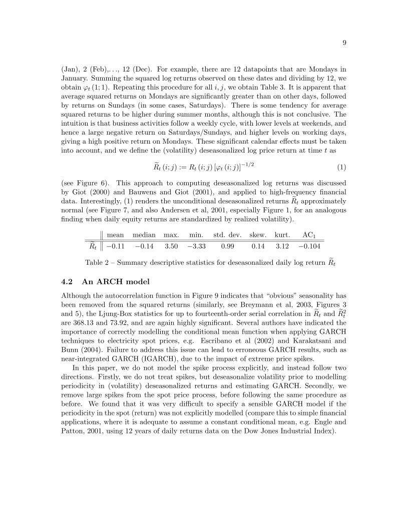
(Jan), 2 (Feb),. . ., 12 (Dec). For example, there are 12 datapoints that are Mondays inJanuary. Summing the squared log returns observed on these dates and dividing by 12, weobtain ϕt (1; 1). Repeating this procedure for all i, j, we obtain Table 3. It is apparent thataverage squared returns on Mondays are significantly greater than on other days, followedby returns on Sundays (in some cases, Saturdays). There is some tendency for averagesquared returns to be higher during summer months, although this is not conclusive. Theintuition is that business activities follow a weekly cycle, with lower levels at weekends, andhence a large negative return on Saturdays/Sundays, and higher levels on working days,giving a high positive return on Mondays. These significant calendar effects must be takeninto account, and we define the (volatility) deseasonalized log price return at time t as

Rt (i; j) := Rt (i; j) [ϕt (i; j)]−1/2 (1)

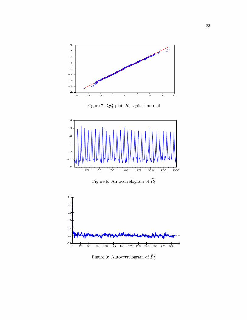
(see Figure 6). This approach to computing deseasonalized log returns was discussedby Giot (2000) and Bauwens and Giot (2001), and applied to high-frequency financialdata. Interestingly, (1) renders the unconditional deseasonalized returns Rt approximatelynormal (see Figure 7, and also Andersen et al, 2001, especially Figure 1, for an analogousfinding when daily equity returns are standardized by realized volatility).

mean median max. min. std. dev. skew. kurt. AC1

Rt −0.11 −0.14 3.50 −3.33 0.99 0.14 3.12 −0.104

Table 2 – Summary descriptive statistics for deseasonalized daily log return Rt

4.2 An ARCH model

Although the autocorrelation function in Figure 9 indicates that “obvious” seasonality hasbeen removed from the squared returns (similarly, see Breymann et al, 2003, Figures 3and 5), the Ljung-Box statistics for up to fourteenth-order serial correlation in Rt and R2

t

are 368.13 and 73.92, and are again highly significant. Several authors have indicated theimportance of correctly modelling the conditional mean function when applying GARCHtechniques to electricity spot prices, e.g. Escribano et al (2002) and Karakatsani andBunn (2004). Failure to address this issue can lead to erroneous GARCH results, such asnear-integrated GARCH (IGARCH), due to the impact of extreme price spikes.

In this paper, we do not model the spike process explicitly, and instead follow twodirections. Firstly, we do not treat spikes, but deseasonalize volatility prior to modellingperiodicity in (volatility) deseasonalized returns and estimating GARCH. Secondly, weremove large spikes from the spot price process, before following the same procedure asbefore. We found that it was very difficult to specify a sensible GARCH model if theperiodicity in the spot (return) was not explicitly modelled (compare this to simple financialapplications, where it is adequate to assume a constant conditional mean, e.g. Engle andPatton, 2001, using 12 years of daily returns data on the Dow Jones Industrial Index).

10

There is little evidence of a significant annual periodicity in the level of deseasonalizedreturns. However, spot prices are clearly higher on weekdays than at the weekend, andthere is evidence that Friday prices are lower than those on Monday to Thursday. Thisdeterministic weekly periodicity is also present in the returns series (Figure 8). We modelthis flexibly using two sinusoidal functions (Figure 10), and the correlogram of the volatilitydeseasonalized returns, filtered to remove weekly periodicity, is given in Figure 11. Theremaining autocorrelation in Rt is captured by including an AR(2) term in Rt. An ARCH-LM(7) test gives the highly significant FARCH = 12.05, and hence we specify the model

Rt = θ0 + θ1 cos[

2π7

(t− θ2)]

+ θ3 cos[

4π7

(t− θ4)]

+ ψ1Rt−1 + ψ2Rt−2 + εt, (2)

where θ0 is the level of the deseasonalized returns, θ1 and θ3 are amplitudes of a 7-day and3 1/2-day sinusoid, θ2 and θ4 are timeshifts, and εt ∼ GARCH(p, q).

We estimated model (2) for p ∈ {0, 1, 2, 3, 4, 5} and q ∈ {0, 1, 2, 3, 4, 5}, using boththe Berndt–Hall–Hall–Hausman and Marquardt optimization routines. Robust QMLEstandard errors are not available. We chose the GARCH model that gave sensible, andsignificant parameter estimates, and which minimized the Schwarz Criterion (SC = 2.3303).Surprisingly, given the prevalence of GARCH-type behaviour in applied finance studies,we found ARCH(1) to be the order which satisfied these conditions, and which generallyconverged after the least iterations, with the more stable Marquardt algorithm. Hence, theconditional variance for deseasonalized returns is

ht = ω + α1ε2t−1, (3)

where εt = εth1/2t are residuals from (2), and εt are Student’s t(r) innovations. The

implication is that the volatility of the deseasonalized returns process is a function ofthe error made in forecasting the previous day’s return. Note that volatility persistenceincreases as α1 approaches unity. Estimated parameters and standard errors are:

ω α1 r

0.4472 0.3273 5.9220(0.0399) (0.0799) (1.3963)

θ0 θ1 θ2 θ3 θ4 ψ1 ψ2

−0.1591 −0.7335 52.9226 −0.4249 −2.3518 −0.3189 −0.0767(0.0233) (0.0358) (0.0627) (0.0350) (0.0475) (0.0348) (0.0301)

and R2 = 0.36. The estimated conditional variance (and other) parameters are all highlysignificant. The adequacy of (2) and (3) was examined using an ARCH–LM(7) test, whichgave an insignificant value of FARCH = 1.29, indicating that all GARCH effects havesuccessfully been removed, and that (2) and (3) track the short-run interdaily volatilitydependencies quite well.

11

We calculate the unconditional variance as hu = ω(1 − α1)−1 = 0.6648, which cor-responds to an average annualized (stochastic component of) volatility of approximately((365)(0.6648))1/2 ≈ 15.6%. The volatility half-life is 0.62 days, which is very mildly per-sistent (a t-test of a unit root in the conditional variance equation gives |τ | = 8.42 > 1.96,and we reject the IGARCH null). This makes intuitive sense, since volatility is driven byshort-term imbalances in demand and supply. It is straightforward to combine (1) and (3)to calculate volatility for the raw returns Rt as (htϕt (i; j))1/2. The in-sample forecastingability of this model is illustrated in Figure 12, where ht is plotted against R2

t (the latteracts as a proxy for ex post volatility).

4.3 The absence of leverage effects

The symmetric relationship between lagged shocks and conditional variance can be illus-trated conveniently using a news impact curve (Engle and Ng, 1993), given directly from(3) as hNIC

t = 0.4472 + 0.3273ε2t−1. We check for the presence of asymmetric GARCH ef-fects using the Engle-Ng sign bias (SB) test, negative and positive size bias (NSB and PSB)tests, and a joint LM test. The SB test examines the possibly asymmetric impacts thatshocks of different sign have on volatility. The NSB (PSB) test investigates the possiblydifferent impacts that negative (positive) shocks of different magnitude have on volatility.We define a dummy variable

S−t ={

1 if εt < 00 if εt ≥ 0

and define negative and positive residuals as ε−t = S−t εt and ε+t =(1− S−t

)εt respectively.

We then estimate (using standardized and ordinary residuals)

ε2t = κ0 + κ1S−t−1 + κ2ε

−t−1 + κ3ε

+t−1 + error, (4)

and test SB, NSB and PSB by using the t-ratios on κ1, κ2, and κ3 in (4),

κ0 κ1 κ2 κ3 κ2 + κ3

1.0740 −0.0718?? 0.0511?? −0.1446?? −0.0935??

(0.1254) (0.1852) (0.1312) (0.1263) (0.1821)

where ?? indicates insignificance at the 10% level, and White’s heteroscedasticity-consistentstandard errors are given in parentheses. The SB, NSB and PSB tests are highly insignifi-cant, which suggests that there are no asymmetric effects. Moreover, a joint LM test of noasymmetry, computed from (4) as TR2 = 0.95 < 7.81 = χ2

0.95 (3) , does not reject the null.We corroborate these findings using asymmetric GARCH. A threshold TGARCH(1,0,1)

extension of (3) was selected, following the same procedure as above, using conditional meanspecification (2), and with Student’s t(r) innovations, i.e. ht = ω + α1ε

2t−1 + λ1S

−t−1ε

2t−1.

Estimated parameter values change slightly, and are not reported here. The “asymme-try” parameter λ1 = 0.0188??(0.1348) is highly insignificant, suggesting that there is no

12

(first-order) leverage effect. Similarly, we selected exponential EGARCH(1,0,1) and powerPGARCH(1,1,1) models. Conditional variance specifications are, with asymmetry param-eters γ1 and φ1, ln(ht) = ω + α1|εt−1h

−1/2t−1 | + γ1εt−1h

−1/2t−1 and h

δ/2t = ω + α1(|εt−1| −

φ1εt−1)δ + β1hδ/2t−1. We find that δ = 3.8315(1.6510), while γ1 = 0.0381??(0.0593) and

φ1 = −0.0038??(0.0715) are again highly insignificant. The conditional variance of thedaily PDA deseasonalized returns does not respond asymmetrically to positive and nega-tive shocks, unlike e.g. asset prices (Nelson, 1991) and interest rates (Chan et al, 1992).

4.4 Spike filtering, volatility forecasts, and long-memory

We identified the 8 spot price dates that exceeded 75 euros/MWh, as Mon 17 – Wed 19Dec 2001, Tue 15 – Wed 16 July 2003, Tue 22 – Wed 23 July 2003, and Mon 11 Aug 2003(the latter represents the extremely large value of 310.37 euros/MWh). For each of thesedates, we replaced the “spikes” with the mean of the spot prices given on the day prior toand following the spike period. We then followed the volatility deseasonalization procedureabove to give a large-spike-filtered ϕt(i; j), where the bold values in Table 3 are changed.Recalculation of Rt and estimation of (2) and (3) gave:

ω α1 r

0.4621 0.2624 6.2780(0.0402) (0.0707) (1.5762)

θ0 θ1 θ2 θ3 θ4 ψ1 ψ2

−0.1508 −0.7636 −3.0668 −0.4351 −2.3337 −0.3411 −0.0838(0.0235) (0.0362) (0.0620) (0.0353) (0.0470) (0.0345) (0.0308)

and R2 = 0.38. An ARCH–LM(7) test gave a borderline value of FARCH = 2.11. Theunconditional variance and half-life of the large-spike-filtered series were calculated to be0.6265 (corresponding to an average annualized - stochastic component of - volatility ofapproximately 15.1%), and 0.52 days. We see that these values are quantitatively verysimilar to those above, and that removal of (even very large) spikes from the spot series doesnot have the same importance as in other studies. We conclude that our deseasonalizationof the returns volatility, and correct specification of the conditional mean, serve to alleviatethe problems that could otherwise require explicit modelling of the spike process.

Andersen and Bollerslev (1998a, 1998b) show that there is no contradiction betweenthe ability of a GARCH model to provide accurate volatility forecasts, and poor predictivepower for daily squared returns. We assess this here, by estimating the Mincer-Zarnowitzequation R2

t = π1 + π2ht + error, for both (a) deseasonalized R2t and (b) large-spike-

filtered deseasonalized R2t . Estimated parameters follow, with White’s standard errors in

13

parentheses:π1(a) π2(a) π1(b) π2(b)0.4345 0.8542 0.3253 1.0686

(0.1243) (0.2016) (0.1579) (0.2692)

Estimated R2 is 0.052(a) and 0.048(b), suggesting that the AR(2)-ARCH(1) model haslow explanatory power, and explains at best 5% of the variability of squared deseason-alized returns (a similar result is obtained by computing the squared sample correlation,corr(•, •)2, between the one-step-ahead daily volatility forecast and an ex post measure ofvolatility, such as |Rt| or R2

t – for example, 100 × corr(ht, |Rt|)2 ≈ (a) 3.9% and (b) 3.2%respectively, confirming the previous findings). Essentially, the difficulty is that daily |Rt|and R2

t are noisy estimates of underlying latent volatility. Andersen and Bollerslev (1998a,1998b) show that use of high-frequency data to construct an improved ex post measure oflatent volatility (such as cumulative absolute intraday returns) explains the paradox, andgreatly increases explanatory power. We do not examine hourly returns data here, sincethese exhibit very complicated intraday season- (and time-of-week-) dependent periodici-ties that would need to be accounted for in a similar spirit to the deseasonalization of dailyreturns, but leave this as an issue for future research.

We also follow Andersen and Bollerslev (1997b, 1998b), in checking whether it is rea-sonable to assume hyperbolic decay of the sample autocorrelation function ACm(•) of R2

t ,in which case fractionally-integrated or long-memory volatility processes may be appropri-ate. It is clear from Figures 4, 5 and 8 that the autocorrelation functions of Rt, R2

t andRt are dominated by intraweek periodicities. This is not the case for the autocorrelationfunction of deseasonalized squared returns (Figure 9). Hence, we estimate the degree offractional integration d simply by fitting a hyperbolic decay to ACm(R2

t ) via the regression

ln(ACm) = ξ0 + ξ1 ln(m) + error, m = 1, . . . ,M,

where d = (ξ1 + 1)/2. We use M = 200 lags, although a more detailed analysis wouldrequire a significantly larger number. Estimated parameters are as follows, with White’sstandard errors in parentheses, and se(d) = se(ξ1)/2:

ξ0 ξ1 d

−2.8114 −0.2111 0.3945(0.2924) (0.0673) (0.0337)

An integrated process of order I(d), where 0 < d < 1/2, will eventually have all positiveautocorrelations ACm, and these will decay at a hyperbolic rate. Since d = 0.3945, thissuggests that ACm(R2

t ) ∼ m2d−1, for m large. This seems to be in contrast to the lowARCH(1) volatility persistence found above. Hence, future work could consider the casefor fractionally-integrated FIGARCH-type extensions of the results in this paper (see e.g.Baillie et al, 1996).

14

5 Conclusions

In this paper, we combine a deterministic multiplicative annual/intraweek pattern for elec-tricity volatility with a sinusoidal intraweek level, and an AR(2)-ARCH(1) model for thestochastic part of returns volatility. This procedure builds upon recent work on intraday fi-nancial data (which has not previously been applied to the unusual volatility that is presentin electricity markets), while taking account of certain stylized features of the market price(notably, weekly seasonality). We find that all estimated parameters are highly significant,and that Powernext PDA electricity volatility is only mildly persistent. Moreover, there areno leverage effects in the stochastic part of volatility, which contrasts sharply with manyresults on “standard” financial series such as asset prices and interest rates. Our workprovides some new insights into the nature, and modelling of, electricity market volatility.

Various extensions of this work are possible, and include (a) modelling the volatility ofhourly spot (returns) data, which will involve treatment of the very complicated (seasonand time-of-week dependent) intraday patterns, (b) further investigation of the volatilitydeseasonalization in this context, including assessment of whether transformation of theunconditional returns to approximate normality is common across different markets, (c)assessment of the aggregational properties of GARCH-type techniques using this data (es-pecially between daily and hourly data), (d) gauging the impact of exogenous variables onelectricity volatility, including temperature and volume, see e.g. Lamoureux and Lastrapes(1990), (e) use of hourly data to provide improved ex post volatility measurements, (f)detailed assessment of possible long-memory dependence in both the spot series, and involatility. We leave these issues for future research.

Acknowledgements The authors are very grateful to Karim Abadir, Michel Culot,Valerie Limpens, Sebastien de Menten, Michael Monoyios and Nikolaos Roupakas for sev-eral discussions and helpful comments during this research. We thank Powernext SA forproviding the daily PDA spot price data. Steve Lawford acknowledges support from Elec-trabel SA, Jacqueline Boucher and Andre Bihain. Spyridon Liarmakopoulos acknowledgessupport from the Department of Economics and Finance, Brunel University. The authorstake full responsibility for all information expressed herein, and for any remaining errors,and the work does not necessarily reflect the views or interests of Electrabel SA, PowernextSA, or Brunel University. This paper was compiled using MiKTeX, and numerical resultswere calculated using EViews.

15

6 References

Andersen T G and Bollerslev T, 1997a, Intraday periodicity and volatility persistence infinancial markets, Journal of Empirical Finance, 4, 115-158.

Andersen T G and Bollerslev T, 1997b, Heterogeneous information arrivals and returnvolatility dynamics: Uncovering the long-run in high-frequency returns, Journal of Fi-nance, 52, 975-1005.

Andersen T G and Bollerslev T, 1998a, Answering the skeptics: Yes, standard volatilitymodels do provide accurate forecasts, International Economic Review, 39, 885-905.

Andersen T G and Bollerslev T, 1998b, Deutsche Mark-Dollar volatility: Intraday ac-tivity patterns, macroeconomic announcements, and longer-run dependencies, Journal ofFinance, 53, 219-265.

Andersen T G, Bollerslev T, Diebold F X and Ebens H, 2001, The distribution of realizedstock return volatility, Journal of Financial Economics, 61, 43-76.

Atkins F J and Chen J, 2002, Some statistical properties of deregulated electricity pricesin Alberta, Department of Economics Discussion Paper 2002–06, University of Calgary.

Baillie R T and Bollerslev T, 1991, Intra-day and inter-market volatility in foreign exchangerates, Review of Economic Studies, 58, 565-585.

Baillie R T, Bollerslev T and Mikkelsen H O, 1996, Fractionally integrated generalizedautoregressive conditional heteroscedasticity, Journal of Econometrics, 74, 3-30.

Barlow M T, 2002, A diffusion model for electricity prices, Mathematical Finance, 12, 287-298.

Barndorff-Nielsen O E and Shephard N, 2002, Econometric analysis of realized volatilityand its use in estimating stochastic volatility models, Journal of the Royal Statistical So-ciety Series B, 64, 253-280.

Barone-Adesi G and Gigli A, 2002, Electricity derivatives, mimeo: Faculty of Economics(Finance), USI.

Bauwens L and Giot P, 2001, Econometric Modelling of Stock Market Intraday Activity(Dordrecht: Kluwer), Advanced Studies in Theoretical and Applied Econometrics, #38.

16

Bera A and Higgins M L, 1993, ARCH models: properties, estimation and testing, Journalof Economic Surveys, 7, 305-366.

Bessembinder H and Lemmon M, 2002, Equilibrium pricing and optimal hedging in elec-tricity forward markets, Journal of Finance, 57, 1347-1382.

Bollerslev T, Chou R Y and Kroner K F, 1992, ARCH modeling in finance: A review ofthe theory and empirical evidence, Journal of Econometrics, 52, 5-59.

Bollerslev T, Engle R F and Nelson D B, 1994, ARCH models, Handbook of Econometricsvol IV, ed R F Engle and D McFadden (Amsterdam: North-Holland) pp 2959-3038.

Borovkova S, 2004, The forward curve dynamic and market transition forecasts, ModellingPrices in Competitive Electricity Markets, ed D W Bunn (Chichester: John Wiley andSons) pp 267-284.

Borovkova S and Permana F J, 2004, Modelling electricity prices by the potential jump-diffusion, paper presented at Stochastic Finance 2004, ISEG, Lisbon.

Bottazzi, G, Sapio S and Secchi A, 2004, A statistical analysis of electricity price fluctua-tions, paper presented at Stochastic Finance 2004, ISEG, Lisbon.

Breymann W, Dias A and Embrechts P, 2003, Dependence structures for multivariate high-frequency data in finance, Quantitative Finance, 3, 1-14.

Carnero M, Koopman S and Ooms M, 2003, Periodic heteroskedastic RegARFIMA modelsfor daily electricity spot prices, Discussion Paper TI 2003–071/4, Tinbergen Institute.

Cartea A and Figueroa M G, 2004, Pricing in electricity markets: A mean reverting jumpdiffusion model with seasonality, mimeo: Birkbeck College, University of London.

Chan K C, Karolyi G A, Longstaff F A and Sanders A B, 1992, An empirical compari-son of alternative models of the short-term interest rate, Journal of Finance, 47, 1209-1227.

Deidersen J and Truck S, 2002, Energy price dynamics: Quantitative studies and stochasticprocesses, Technical Report TR–ISWM–12/2002, Universitat Karlsruhe.

Engle R F, 2001, GARCH 101: The use of ARCH/GARCH models in applied economet-rics, Journal of Economic Perspectives, 15, 157-168.

17

Engle R F, 2002, New frontiers for ARCH models, Journal of Applied Econometrics, 17,425-446.

Engle R F, 2004, Risk and volatility: Econometric models and financial practice, AmericanEconomic Review, 94, 405-420.

Engle R F and Ng V K, 1993, Measuring and testing the impact of news on volatility,Journal of Finance, 48, 1749-1778.

Engle R F and Patton A J, 2001, What good is a volatility model?, Quantitative Finance,1, 237-245.

Escribano A, Pena J I and Villaplana P, 2002, Modelling electricity prices: Internationalevidence, Economics Series Working Paper 08: 02–27, Universidad Carlos III de Madrid.

Eydeland A and Geman H, 2000, Fundamentals of Electricity Derivatives, in: Energy Mod-eling and the Management of Uncertainty (London: Risk Publications).

Geman H and Roncoroni A, 2006, Understanding the fine structure of electricity prices,Journal of Business, 79, forthcoming.

Giot P, 2000, Time transformations, intraday data, and volatility models, Journal of Com-putational Finance, 4, 31-62.

Haldrup N and Nielsen M, 2005, A regime switching long memory model for electricityprices, Journal of Econometrics, forthcoming.

Harris L, 1986, A transaction data study of weekly and intradaily patterns in stock returns,Journal of Financial Economics, 16, 99-117.

Huisman R and Mathieu R, 2003, Regime jumps in electricity prices, Energy Economics,25, 425-434.

Joskow P L, 1997, Restructuring, competition and regulatory reform in the U.S. electricitysector, Journal of Economic Perspectives, 11, 119-138.

Karakatsani N V and Bunn D W, 2004, Modelling stochastic volatility in high-frequencyspot electricity prices, mimeo: Department of Decision Sciences, London Business School.

Knittel C R and Roberts M R, 2004, An empirical examination of restructured electricityprices, mimeo: Department of Economics, University of California–Davis.

18

Koekebakker S and Ollmar F, 2001, Forward curve dynamics in the Nordic electricitymarket, Discussion Paper 2001–21, Department of Finance and Management Science, Nor-wegian School of Economics and Business Administration.

Lamoureux C G and Lastrapes W D, 1990, Heteroskedasticity in stock return data: Vol-ume versus GARCH effects, Journal of Finance, 45, 221-229.

Li W K, Ling S and McAleer M, 2002, Recent theoretical results for time series modelswith GARCH errors, Journal of Economic Surveys, 16, 245-269.

Longstaff F A and Wang A W, 2004, Electricity forward prices: A high-frequency empiricalanalysis, Journal of Finance, 59, 1877-1900.

Lucia J J and Schwartz E S, 2002, Electricity prices and power derivatives: Evidence fromthe Nordic power exchange, Review of Derivatives Research, 5, 5-50.

Manoliu M and Tompaidis S, 2002, Energy futures prices: Term structure models withKalman filter estimation, Applied Mathematical Finance, 9, 21-43.

Mork E, 2001, Emergence of financial markets for electricity: A European perspective,Energy Policy, 29, 7-15.

Nelson D B, 1991, Conditional heteroscedasticity in asset returns: A new approach, Econo-metrica, 59, 347-370.

Pilipovic D, 1998, Energy Risk: Valuing and Managing Energy Derivatives (New York:McGraw-Hill).

Resta M, 2004, Multifractal analysis of power markets: Some empirical evidence, mimeo:School of Economics (Financial Mathematics), University of Genova.

Resta M and Sciutti D, 2003, Spot price dynamics in deregulated power markets, mimeo:School of Economics (Financial Mathematics), University of Genova.

Routledge B R, Seppi D J and Spatt C S, 2001, The “spark spread”: An equilbrium modelof cross-commodity price relationship in electricity, mimeo: Graduate School of IndustrialAdministration, Carnegie Mellon University.

Schwartz E S, 1997, The stochastic behaviour of commodity prices: Implications for valu-ation and hedging, Journal of Finance 52, 923-973.

19

Simonsen I, 2003, Measuring anti-correlations in the Nordic electricity spot market bywavelets, Physica A, 322, 597-606.

Vahvilainen I, 2002, Basics of electricity derivatives pricing in competitive markets, Ap-plied Mathematical Finance, 9, 45-60.

Weron R, 2000, Energy price risk management, Physica A, 285, 127-134.

Weron R, Bierbrauer M and Truck S, 2004, Modeling electricity prices: Jump diffusion andregime switching, Physica A, 336, 39-48.

Weron R and Przyby lowicz B, 2000, Hurst analysis of electricity price dynamics, PhysicaA, 283, 462-468.

Wilkinson L and Winsen J, 2002, What we can learn from a statistical analysis of electric-ity prices in New South Wales, Electricity Journal, April, 60-69.

Wood R A, McInish T H and Ord J K, 1985, An investigation of transaction data forNYSE stocks, Journal of Finance, 25, 723-739.

20

Jan Feb Mar Apr May JunMon 0.172549 0.153134 0.203704 0.362829 0.410702 0.634206Tue 0.150761 0.021786 0.012664 0.167280 0.076427 0.346457Wed 0.093718 0.006296 0.014559 0.010824 0.037801 0.065023Thu 0.084144 0.018015 0.015025 0.007921 0.280272 0.064096Fri 0.039971 0.033769 0.017683 0.014563 0.094877 0.067420Sat 0.102417 0.048805 0.049265 0.048285 0.105214 0.190565Sun 0.062880 0.034773 0.074696 0.255434 0.142691 0.173772

Jul Aug Sep Oct Nov DecMon 0.544370 1.301646 0.358908 0.355290 0.466470 0.451605Tue 0.122955 0.516680 0.075058 0.017599 0.030139 0.067990Wed 0.043689 0.014402 0.031409 0.007924 0.032166 0.052622Thu 0.115656 0.052249 0.008192 0.019330 0.017346 0.146491Fri 0.046879 0.029561 0.003446 0.035347 0.039659 0.073754Sat 0.100539 0.078190 0.109275 0.094008 0.220945 0.081298Sun 0.125789 0.117001 0.116502 0.077310 0.143587 0.190638

Table 3. Mean value ϕt(i; j) of squared log daily returns on day i and month j,

where values in bold change following removal of the 8 largest spikes from thespot (returns) series – new values are not reported here.

21

Figure 1: Spot St (27.11.01-21.06.04)

Figure 2: Return Rt (28.11.01-21.06.04)

Figure 3: QQ-plot, Rt against normal

22

Figure 4: Autocorrelogram of Rt

Figure 5: Autocorrelogram of R2t

Figure 6: Return Rt (28.11.01-21.06.04)

23

Figure 7: QQ-plot, Rt against normal

Figure 8: Autocorrelogram of Rt

Figure 9: Autocorrelogram of R2t

24

Figure 10: Estimated weekly periodicity in Rt, over 14 days

Figure 11: Autocorrelogram of Rt, weekly periodicity removed using sinusoids

Figure 12: Static AR(2)-ARCH(1) forecast, against R2t (28.11.01-21.06.04)