U.U.D.M. Project Report 2015:15

Examensarbete i matematik, 30 hpHandledare och examinator: Erik EkströmJuni 2015

Department of MathematicsUppsala University

Volatility Derivatives – Variance and VolatilitySwaps

Joakim Marklund and Olle Karlsson

Abstract

We give a comprehensive overview of volatility derivatives includingthe history behind it, the applications as well as pricing proceduresin various models. Given these models we also apply market datato approach some empirical evidence, estimating and evaluating theperformance of the models in the frame of variance and volatility swaps.

1

Contents

1 Introduction 41.1 Purpose and Goals . . . . . . . . . . . . . . . . . . . . . . . . 41.2 Structure of Thesis . . . . . . . . . . . . . . . . . . . . . . . . 4

2 History 62.1 Option Pricing and Modelling . . . . . . . . . . . . . . . . . . 62.2 Volatility Trading . . . . . . . . . . . . . . . . . . . . . . . . . 7

3 Volatility Derivatives 93.1 Swaps . . . . . . . . . . . . . . . . . . . . . . . . . . . . . . . 103.2 Variance Swaps . . . . . . . . . . . . . . . . . . . . . . . . . . 10

3.2.1 Example of a Variance Swap . . . . . . . . . . . . . . 113.2.2 Pricing and Valuation . . . . . . . . . . . . . . . . . . 113.2.3 Replicating Approach: First Steps . . . . . . . . . . . 133.2.4 Replicating Approach: Final Steps . . . . . . . . . . . 153.2.5 Discrete Approximation . . . . . . . . . . . . . . . . . 163.2.6 Limitations in Accuracy and Performance . . . . . . . 18

3.3 Volatility Swaps . . . . . . . . . . . . . . . . . . . . . . . . . 193.3.1 Example of a Volatility Swap . . . . . . . . . . . . . . 193.3.2 Pricing . . . . . . . . . . . . . . . . . . . . . . . . . . 193.3.3 Laplace Transforms . . . . . . . . . . . . . . . . . . . 21

4 Jump Diffusion Model 224.1 Jump Dynamics . . . . . . . . . . . . . . . . . . . . . . . . . 234.2 The Effect of Jumps . . . . . . . . . . . . . . . . . . . . . . . 24

5 Stochastic Volatility Models 275.1 The Heston Model . . . . . . . . . . . . . . . . . . . . . . . . 285.2 The GARCH Model . . . . . . . . . . . . . . . . . . . . . . . 295.3 The 3/2 Model . . . . . . . . . . . . . . . . . . . . . . . . . . 315.4 Variance Swaps . . . . . . . . . . . . . . . . . . . . . . . . . . 325.5 Volatility Swaps . . . . . . . . . . . . . . . . . . . . . . . . . 33

5.5.1 PDE Approach . . . . . . . . . . . . . . . . . . . . . . 345.5.2 Laplace Transforms . . . . . . . . . . . . . . . . . . . 35

5.6 Comparison of the Models . . . . . . . . . . . . . . . . . . . . 365.7 Stochastic Volatility Models with Jumps . . . . . . . . . . . . 37

5.7.1 Stochastic Volatility with Jumps in the Underlying(SVJ) . . . . . . . . . . . . . . . . . . . . . . . . . . . 37

5.7.2 Stochastic Volatility with Jumps in Stock Price andVolatility (SVJJ) . . . . . . . . . . . . . . . . . . . . . 38

5.8 Variance Options . . . . . . . . . . . . . . . . . . . . . . . . . 39

2

6 Parameter Calibrations 426.1 European Options . . . . . . . . . . . . . . . . . . . . . . . . 42

6.1.1 Filtering Process . . . . . . . . . . . . . . . . . . . . . 426.2 Option-Based Calibration . . . . . . . . . . . . . . . . . . . . 436.3 B-S Estimation . . . . . . . . . . . . . . . . . . . . . . . . . . 446.4 MJD Estimation . . . . . . . . . . . . . . . . . . . . . . . . . 446.5 Heston Estimation . . . . . . . . . . . . . . . . . . . . . . . . 456.6 The 3/2 Estimation . . . . . . . . . . . . . . . . . . . . . . . 466.7 Price-Based Calibration . . . . . . . . . . . . . . . . . . . . . 476.8 GARCH Estimation . . . . . . . . . . . . . . . . . . . . . . . 48

7 Empirical Evidence 507.1 Variance Swaps . . . . . . . . . . . . . . . . . . . . . . . . . . 507.2 Volatility Swaps . . . . . . . . . . . . . . . . . . . . . . . . . 52

8 Concluding Remarks 55

9 Extensions and Further Research 56

10 Appendix 5810.1 A - Compound Poisson Process . . . . . . . . . . . . . . . . . 5810.2 B - Brockhaus-Long Convexity Approximation . . . . . . . . 58

3

1 Introduction

In terms of finance volatility has always been considered a key measure. Thedevelopment and growth of the financial market over the last centuries havecaused the role of volatility to change. Instead of being just a component inpricing theory it has evolved into an asset class of its own. Volatility deriva-tives in general is a specialized financial tool which gives the opportunity totrade on the volatility of an underlying asset. Several derivatives have beencreated which puts great emphasis on volatility, providing a direct exposureto one of the most common measures of risk. Ever since the mid-1990s, se-curities such as variance/volatility swaps as well as futures and options haveprovided a good approach for investors to trade future realized variance orvolatility against the current implied counterpart.

Who trades in volatility? For the same reason as stock investors tries topredict the movements of the stock market or bond investors think they canforesee the direction of interest rates, one may think they know somethingabout the future volatility levels. If one thinks current volatility is highthere are several derivatives in which one can take a position which profitsif the volatility decreases.

1.1 Purpose and Goals

Our purpose for this thesis is to do an extensive study in the financial areaknown as volatility derivatives, and apply some of the most popular modelsto these derivatives. Mainly focused around the variance and volatility swap,we include the standard Black-Scholes model, the Merton Jump Diffusionmodel as well as Stochastic Volatility Models such as GARCH, Heston and3/2 in order to give a comprehensive study on the evaluation and perfor-mance of these swaps.

The goal is to analyze and compare the different models in a volatility basedsetting. We will use empirical studies based on options as well as historicaldata on the famous S&P500 index and translate the calibrations into ourmodels, where we can explicitly compare them against each other.

1.2 Structure of Thesis

In this paper we will present multiple trading tools which emphasises onvolatility. We start out in chapter 2 by going over the history of volatilityderivatives, giving a brief overview of the growth and development. Movingon we will in chapter 3 derive and present some of the easier contracts usedwhen trading volatility, namely the variance and volatility swaps. We willalso price and evaluate a variance swap in a semi model-independent setting.

4

Options play a significant role in finance, and will naturally have manyuseful purposes even in volatility trading. The famous model for optionpricing which can generate closed-form formulas for options, The Black-Scholes model, have been shown to have certain drawbacks in the way theysimplify the reality. One way to find better empirical support have been toallow jumps in the model, and we will in chapter 4 look into these effectsand variants. To relax the assumption about constant volatility the usualanswer is applying a stochastic volatility model. This popular area has alot of different models which can be applied, and we will derive a couple ofthem. Thus we will in chapter 5 explore the realm of stochastic volatilitymodels.

Looking at several models throughout the paper we will towards the endat chapter 6 and 7 present some empirical evidence in order to fully com-pare and evaluate the differences between the models alongside some relevantanalysis. Finally we conclude in chapter 8 and 9 with our findings and reflecton some possible future research and extensions.

5

2 History

2.1 Option Pricing and Modelling

One of the main reasons that financial mathematics have become an inter-esting subject in the world today can be explained by two words, optionpricing. The concept of buying or selling various commodities in order tomake money off of it has always been a compelling aspect to humans. In ourcontrast the important question is whether or not the market can determinea unique price for every given option, and is this price explicitly computed?The ones to come up with a valid answer to this question was Nobel prizewinners Robert Merton and Myron Scholes in the 1970s (together with Fis-cher Black, who unfortunately had passed away when Merton and Scholeswere awarded the Nobel prize). Their model, the famous Black-Scholesmodel, is the market convention when referring to standard option valua-tions. This model can be put into an explicit formula to determine the priceof European options.

Although innovative and very elegant at the time, the Black-Scholes-Mertonmodel has been criticized because of its limitations and possible defects. Themodel in itself is made fairly simple, and only provides a fair approximationto the real world. But with simplicity comes not only easy implementations,but also certain drawbacks. Some of the assumptions made, the simplifica-tions of reality, might not be fully accurate and the model does not alwaysempirically support the market. Assumptions made such as efficient mar-kets, liquidity or no transaction costs are hard to relax, but some of theassumptions made in the B-S model could be taken off by doing some ex-tensions.

The continuity of the stock returns are aimed to behave in a nice continuousway dictated by the geometric Brownian motion, something that has beenquestionable. Empirically the stock returns have exhibited jumps, meaningthat they over a small time period can experience drastic changes. To dealwith this phenomenon the solution have been to introduce a jump processinto the original model, where the most famous extension being the MertonJump Diffusion model.

One assumption that have been questioned and criticized include that wehave a constant volatility (σ). To be able to relax this assumption one oftenmoves over to stochastic volatility models. The difference being that weno longer assumes constant volatility, but that it follows a random processgiven by some dynamics. Examples of such models that have been seento give better empirical support include the Heston model or the GARCH(Generalized Autoregressive Conditional Heteroskedasticity) model.

6

Another important assumption of the B-S model is that we have Gaus-sian log-increments of the stock price. Studies over the years of stock priceshave shown that the usage of the Gaussian model is incompatible due toevidence of heavy tails empirically, which suggests that it might be morereasonable to replace the Brownian motion with a more general family thatremoves the faulty assumptions, for example a Levy process. [1]

2.2 Volatility Trading

Volatility derivatives started to appear in the late 20th century. At this timethe contract that first saw its light was a variance swap, and were dealt at theUBS investment bank in Switzerland in 1993 by Michael Weber. The vari-ance swaps were rather illiquid during the first years, but increased heavilyafter 1998 and has ever since the millennia become a credible trading tool.Thanks to the development of the replicating argument which involves us-ing a portfolio of vanilla options to properly replicate a variance swap, themarket for volatility grew even larger. [8]

Although the popularity of these volatility derivatives have evolved sinceits introduction and is nowadays seen as an asset class in it owns right anda tradable market instrument, there has been downfalls. The Wall StreetJournal reported during the financial crisis in 2008 that the extreme volatil-ity levels almost killed the market for volatility swaps. [37] The unforeseenextremes made traders unable to hedge volatility reliably. In this period oftime the liquidity became very scarce and trading in this niched area dimin-ished significantly and was reduced to ”trade by appointment”.

A famous volatility symbol is the Volatility Index (denoted VIX), a volatil-ity index operated by the Chicago Board Options Exchange (CBOE). In-troduced in 1993, this volatility index have been a popular measure of theimplied volatility, and measures expectations of volatility over 30 day pe-riods. It started off by replicating the one-month implied volatility on theS&P100 index, and expanded in 2003 to measure market expectations ofvolatility conveyed by the S&P500 stock index. The VIX index has sinceits introduction been considered the world’s benchmark for stock marketvolatility. The introduction of this index has laid a good foundation for thedevelopment and interest in volatility products and speculating in volatil-ity derivatives. Over the years the CBOE has launched a futures exchange(CFE) as well as allowing trades on VIX options to enlarge the family ofvolatility derivatives. The figure below maps the evolution of the VIX index,an index also known as the ”fear index” or ”risk index”.

7

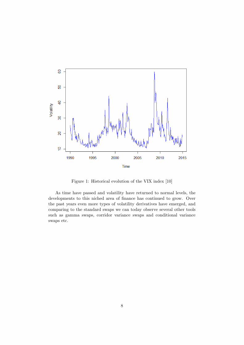
Figure 1: Historical evolution of the VIX index [10]

As time have passed and volatility have returned to normal levels, thedevelopments to this niched area of finance has continued to grow. Overthe past years even more types of volatility derivatives have emerged, andcomparing to the standard swaps we can today observe several other toolssuch as gamma swaps, corridor variance swaps and conditional varianceswaps etc.

8

3 Volatility Derivatives

Volatility derivatives are a special type of financial derivative where the pay-off will depend on the volatility of an underlying asset. Some of the mostcommon examples in this area are variance and volatility swaps or optionswritten on the volatility index, VIX.

Trading in volatility derivatives have become popular in risk managementdue to its direct exposure to the volatility. Thus with these types of finan-cial derivatives volatility is now a tradable market instrument. In the pasttraders would normally use a delta-hedged position to trade with volatility.This however does not perfectly trade with volatilities alone, since the re-turn also is dependent of the underlying stock price. The introduction tovariance and volatility swaps have provided a pure exposure to volatility,making it popular when interested in these circumstances. [26]

Why trade in volatility over regular financial derivatives? Volatility as atrading tool have several characteristics which makes trading it attractive.Although there is technically possible to achieve a variance swap payoff withvanilla options, a natural question becomes why should one be encouragedto trade in volatility compared to other financial tools. The easiest answeris that a these tools offers direct exposure to volatility, removing the pathdependency issues that comes when delta-hedging an option. Trading inregular options the investor has to both be aware of the underlying price aswell as how the volatility changes, something that a pure volatility traderdoesn’t. Some of the most common reasons are listed below:

• Speculative position: Here the investor takes a directional positionin the volatility of an underlying. If one believes that current volatil-ity levels are incorrect or that the expectation of future volatility ishigh/low one can utilize volatility derivatives to make a profit. Ex-amples of such situations include political or financial turmoil due tocurrent debt issues or belief in changes due to a forthcoming election.

• Hedging position: Looking at a hedging perspective there is a va-riety of industries that trades in volatility as part of their portfolio.Volatility is often found to be negatively correlated with a stock orindex level, making hedging in volatility a good diversification strat-egy. During market crashes volatility is generally known to increase, anphenomenon knows as Black’s leverage effect [4], which makes hedgingin volatility during those times a means to reduce losses.

9

3.1 Swaps

Introduced in the 1980s, a swap is an agreement between two counterpartsto exchange cash flows in the future. The agreement will define which datesthe cash flows will be paid as well as how they will be calculated. One partyagrees to pay a fixed amount to the other counterpart which in return acceptsthe agreement by paying a floating amount, an amount which depends on theunderlying. A swap is an OTC product (Over-The-Counter), and the mostcommon types of swaps are for example interest rate swaps and currencyswaps. The focus of this thesis will be on the swaps written on variance andvolatility. These swaps allows the investor a direct position in volatility orvariance of a stock index or a specific stock. These type of swaps generallyonly have a single payment at expiration, which is not always the case whendealing in other swaps.

3.2 Variance Swaps

A forward contract where one counterparty agrees to pay a notional amount,call it N , times the difference between a fixed level of variance and a realizedamount. For variance swaps the fixed level is usually called variance strikeprice. The realized variance is determined by calculating the variance of theassets return over the lifespan of the swap.

To calculate the realized variance we need a couple of variables, which in-cludes the observation frequency of the price of the underlying, the annual-ization factor and the method of calculating the variance. It is importantthat the procedure of calculating these variables are clearly specified beforeentering a swap. For example whether the standard deviation of returnsis calculated by assuming a zero mean or not. When dealing with discretesampling we create a partition 0 = t0 < t1 < ... < tn = T of the timeinterval [0, T ], thus creating n equal segments with lengths ∆t (ti = iT/n).Given all this information we define the realized variance in these types ofcontracts by the formula

Vd(0, n, T ) =AF

n− 1

n−1∑i=0

(log(Si+1

Si

))2. (1)

Here n is the number of return observations, Si is the price of the asset attime ti and AF stands for the annualization factor. AF , defined by n/T ,would be 252 if the maturity of the swap were 1 year with daily sampling(T = 1, n = 252). Thus the variance swap payoff is defined as

(Vd(0, n, T )−Kvar)×N (2)

where Vd(0, n, T ) is defined as above, N is the notional amount and Kvar isthe variance strike.

10

3.2.1 Example of a Variance Swap

To get a better grasp of how the variance swap works, we proceed with asimple made up example. Worth mentioning before we start is that the vari-ance strike price is usually quoted in units of volatility squared, e.g. (15%)2.

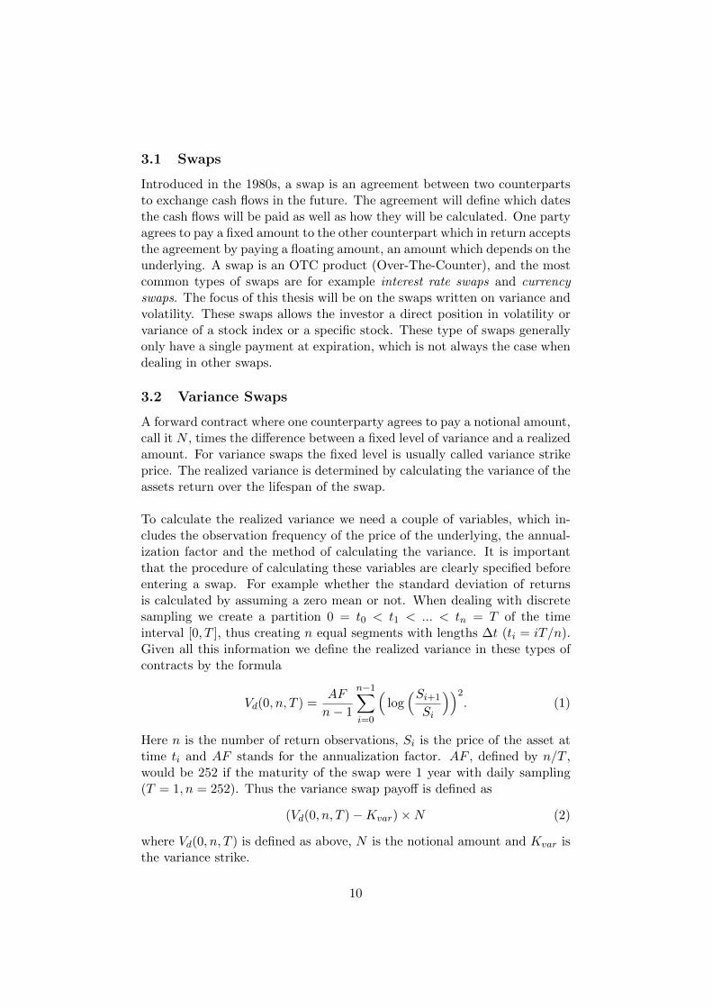
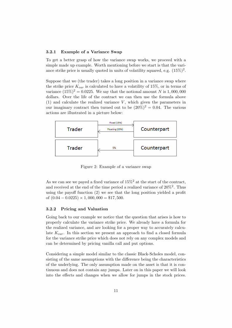
Suppose that we (the trader) takes a long position in a variance swap wherethe strike price Kvar is calculated to have a volatility of 15%, or in terms ofvariance (15%)2 = 0.0225. We say that the notional amount N is 1, 000, 000dollars. Over the life of the contract we can then use the formula above(1) and calculate the realized variance V , which given the parameters inour imaginary contract then turned out to be (20%)2 = 0.04. The variousactions are illustrated in a picture below:

Figure 2: Example of a variance swap

As we can see we payed a fixed variance of 15%2 at the start of the contract,and received at the end of the time period a realized variance of 20%2. Thususing the payoff function (2) we see that the long position yielded a profitof (0.04− 0.0225)× 1, 000, 000 = $17, 500.

3.2.2 Pricing and Valuation

Going back to our example we notice that the question that arises is how toproperly calculate the variance strike price. We already have a formula forthe realized variance, and are looking for a proper way to accurately calcu-late Kvar. In this section we present an approach to find a closed formulafor the variance strike price which does not rely on any complex models andcan be determined by pricing vanilla call and put options.

Considering a simple model similar to the classic Black-Scholes model, con-sisting of the same assumptions with the difference being the characteristicsof the underlying. The only assumption made on the asset is that it is con-tinuous and does not contain any jumps. Later on in this paper we will lookinto the effects and changes when we allow for jumps in the stock prices.

11

For now the asset takes the following characteristics:

dSt = µ (t, ...)Stdt+ σ (t, ...)StdWt. (3)

Here, we assume that the drift µ and the volatility σ are arbitrary func-tions of time and other parameters. These assumptions include, but arenot limited to, models in which the volatility is a function of stock priceand time only (σ (t, St)). While we denoted the discrete realized variance asVd(0, n, T ) we will naturally let the continuous sampled realized variance bedenoted by Vc(0, T ). This is a theoretical element representing the averagecombined fluctuations of the volatility and is defined as

Vc(0, T ) =1

T

∫ T

0σ2 (s, ...) ds. (4)

The discrete realized variance defined in the previous section, or the so calledfloating leg of the swap, will in the limit approach the continuous realizedvariance. This means that we have the relationship

Vc(0, T ) = limn→∞

Vd(0, n, T ). [26] (5)

To justify this relation we begin by looking at Vd (0, n, T ) (recall equation

(1)), and substituting the solution St = S0 exp(∫ t

0

(µ− σ2

2

)ds+

∫ t0 σdWs

)into the discrete realized variance. Recall that we also have that AF = n/T .This yields that

limn→∞

Vd(0, n, T ) =

limn→∞

n

T (n− 1)

n−1∑i=0

(∫ ti+1

ti

(µ− σ2

2

)ds+

∫ ti+1

ti

σdWs

)2

.(6)

Here we consider σ and µ to be simple processes, recall that if they are notsimple we can approximate them with simple processes. Calculating thesquare above and evaluating we arrive at

limn→∞

n

T (n− 1)

n−1∑i=0

σ2(Wti+1 −Wti

)2+Ri = Vc(0, T ). (7)

Here we see that under the limit the first sum converges to our definitionof Vc (0, T ) and the rest term Ri converges to zero since it consists of termswith

∑n−1i=0 ai (ti+1 − ti)2 and

∑n−1i=0 bi (ti+1 − ti)

(Wti+1 −Wti

)where ai and

bi are some constants.

Having defined the necessary tools for this model we start by looking at thecorresponding price process of a variance swap Π (t,N (Vc −Kvar)). This

12

process are solved using the Feynman-Kac formula, which gives a solutionof the form

Π (t,N (Vc −Kvar)) = EQt

[e−r(T−t)N (Vc (t, T )−Kvar)

]. (8)

As we assume a lack of arbitrage in the market we can conclude that at thetime of signing the net worth of the contract has to be zero. This assump-tion thus implies that the continuous variance strike price must satisfy theequation

Kvar = EQ0 [Vc (0, T )] = EQ0

[1

T

∫ T

0σ2dt

]. (9)

Thus we have found a valid approach of what the variance strike shouldbe. This approach is a good idea for valuating the contract but does nothowever give a good interpretation in how to properly calculate it. In orderto replicate the contract we then look into a method involving a rebalancingstrategy of a stock as well as a log contract, a method which caused a bigoutburst in the area of volatility derivatives.

3.2.3 Replicating Approach: First Steps

To start off the replicating strategy we use Ito’s lemma on a theoreticallog contract of the underlying asset which yields the stochastic differentialequation

d (logSt) =

(µ− σ2

2

)dt+ σdWt. (10)

In order to achieve a plausible result we combine 1/St contracts of the assetas well as being short in the aforementioned log contracts we arrive at thevery useful equation

dStSt− d (logSt) =

σ2

2dt. (11)

With the use of this technique we can see that the drift µ has been cancelled,which is what we were trying to obtain. Writing this as an integral equationfrom 0 to T multiplied with the constant 1/T and rearranging we get a newformula for the theoretical realized variance

1

T

∫ T

0σ2dt =

2

T

(∫ T

0

dStSt− log

(STS0

)). (12)

Recall here that the variance strike price Kvar was equal to the expectedvalue of the theoretical realized variance in equation (9). Thus to proceedwe have to calculate the expected values of these contracts in order to geta solution formula for Kvar. This means that our variance strike will havethe form:

Kvar =2

TE

[∫ T

0

dStSt− log

(STS0

)]. (13)

13

Thus to solve this we need to calculate the respective expected values. Firstwe note that as we are working with a risk neutral measure the asset willtake a slightly new form as

dSt = rStdt+ σ (t, ...)StdWt. (14)

Here r stands as usual for the risk free interest rate, and will be assumedconstant. Given these characteristics we are now ready to calculate theexpected values. For the first set of contracts we can easily evaluate thisand through standard calculations we have

EQ0

[∫ T

0

dStSt

]= rT. (15)

Next up we need to replicate the log contract, which is a bit harder andcan be done by statically using vanilla call and put options. We do this byletting f be a twice differentiable function which will represent a payoff ofa European style path-independent derivative security. Such a function canbe expressed in accordance of Breeden and Litzenberger (1978, [5]) as:

f(ST ) = f(x) + f ′(x)(ST − x)

+

∫ x

0f ′′(K)(K − ST )+dK +

∫ ∞x

f ′′(K)(ST −K)+dK.(16)

The formula above can be obtained by using integration by parts on

f(s)− f(x) =

∫ s

xf ′(t)dt = f ′(x)(s− x) +

∫ s

xf ′′(t)(s− t)dt. (17)

Rewriting the last integral with an indicator function and dividing it intotwo different integrals makes us arrive at the required formula. Then thepayoff function f could be replicated by holding different positions on a zerocoupon bond (with face value f(x)), a forward contract with strike price xas well as call and put options. As we are interested in the zero value ofthe claim, we can express this in terms of standard European call and putoptions denoted C(K) and P (K) respectively with maturities at time T andstrike price K. Calculating the expected values at time zero and discountingfor our function f(ST ) we have

EQ0 [e−rT f(ST )] = e−rT f(x) + f ′(x)[C(x)− P (x)]

+

∫ x

0f ′′(K)P (K)dK +

∫ ∞x

f ′′(K)C(K)dK.(18)

With this equation we just need to transfer back the payoff function finto our log contract in order to fully replicate the variance swap. Let-ting f(ST ) = log(ST /S∗) and x = S∗, where S∗ > 0 is some arbitrary cutoff

14

in order to separate the call and put options, as well as substituting thisinto equation (16) we get:

log

(STS∗

)=ST − S∗S∗

−∫ S∗

0

1

K2(K−ST )+dK−

∫ ∞S∗

1

K2(ST−K)+dK. (19)

One important note here is that the log contract above is not the exact sameas the one we looked at in equation (12). It should be noted that we canrewrite the log payoff as

logSTS0

= logSTS∗

+ logS∗S0. (20)

The first term in the equation above is the one we have replicated in (19),and the second one is a constant term which is independent of the final stockprice ST . Given that we have replicated the first term and the second termis constant we are now ready to move forward and put everything together.

3.2.4 Replicating Approach: Final Steps

Up to this point we have seen how to handle both the rebalanced hedge of1/St and the log contract. To finish off the replicating strategy we need toput together both those terms. What we have obtained without expectationsis

Vc(0, T ) =2

T

[∫ T

0

dStSt− ST − S∗

S∗− log

(S∗S0

)+

+

∫ S∗

0

1

K2P (K)dK +

∫ ∞S∗

1

K2C(K)dK

].

(21)

Going back to equation (9) we need to calculate the expected values of theabove equation to obtain a solution formula for the variance strike price,Kvar. This yields that

Kvar =2

T

[rT −

(S0S∗erT − 1

)− log

(S∗S0

)+

+ erT∫ S∗

0

1

K2P (K)dK + erT

∫ ∞S∗

1

K2C(K)dK

] (22)

where S0 is the initial price of the underlying, S∗ is the positive arbitrarycutoff and C(K) as well as P (K) are vanilla European call and put optionswith strike prices K. One interesting note is that if we were to choose thecutoff as S∗ = S0e

rT we could reduce the equation of the variance strikeabove into a simpler form of

Kvar =2erT

T

[∫ S0erT

0

1

K2P (K)dK +

∫ ∞S0erT

1

K2C(K)dK

]. (23)

15

3.2.5 Discrete Approximation

As we saw earlier we can replicate a variance swap by a portfolio of vanillaoptions, and we didn’t require any particular model assumption to deter-mine the variance strike price. For a discrete approximation of the repli-cating scheme the only complicated task resides in how to compute the calland put options, which means that we have to find a reasonable approachto replicate the log contract. For this approximation we have chosen so thatthe cutoff is equal to the initial stock price (S∗ = S0).

Following the frameworks of Demeterfi et al. (1999, [13]), we will checkif our initial approach can match the reality which only requires the usageof a discrete set of options. To properly replicate the aforementioned logcontract in terms of standard European options we remind ourselves withthe definition of the variance strike by equation (13), which can be rewrittenas

Kvar =2

TE

[∫ T

0

dStSt− ST − S∗

S∗− log

(S∗S0

)+ST − S∗S∗

− log

(STS∗

)].

Taking expectations of the equations above we will have a variance strikeprice of

Kvar =2

T

[rT −

(S0S∗erT − 1

)− log

(S∗S0

)]+ erTΠCP (24)

Here we then have a term which can be instantly calculated through thechoices in cutoff, time of maturity, rate etc. The function ΠCP will denotethe present value of the portfolio with vanilla options, and has a payoff atexpiration given by

f(ST ) =2

T

[ST − S∗S∗

− logSTS∗

]. (25)

In practice we are only able to use a discrete set of option to replicate this,and we need to determine how to appropriately set this up. Lets assumethat we are able to trade call options with strikes

K0 = S∗ < K1c < K2c < ... (26)

as well as put options with strikes

K0 = S∗ > K1p > K2p > ... (27)

By a piece-wise linear approximation we can determine how many optionsof each particular strike we will put into the portfolio. As an example, for acall option with strike price K0 we would have

wc(K0) =f(K1c)− f(K0)

K1c −K0. (28)

16

The following segment will then be a combination of strikes K0 and K1c:

wc(K1) =f(K2c)− f(K1c)

K2c −K1c− wc(K0). (29)

Continuing in a similar fashion one can build the entire payoff curve, onestep at a time. The general formula for the weights for call and put optionsis thus

wc(Kn,c) =f(Kn+1,c)− f(Kn,c)

Kn+1,c −Kn,c−n−1∑i=0

wc(Ki,c) (30)

wp(Kn,p) =f(Kn+1,p)− f(Kn,p)

Kn,p −Kn+1,p−n−1∑i=0

wp(Ki,p). (31)

As seen above the principle for calculating put options is done in a similarfashion as the call options. Once we have calculated the weights from theframework above we can then obtain ΠCP from

ΠCP =∑i

w(Kip)P (S,Kip) +∑i

w(Kic)C(S,Kic). (32)

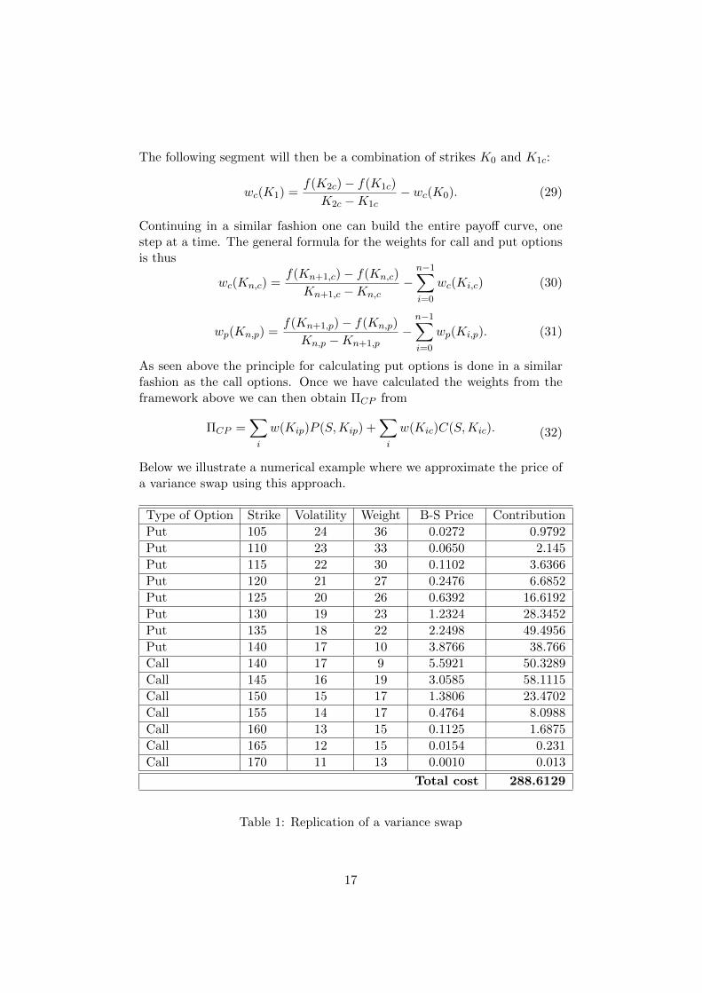
Below we illustrate a numerical example where we approximate the price ofa variance swap using this approach.

Type of Option Strike Volatility Weight B-S Price Contribution

Put 105 24 36 0.0272 0.9792

Put 110 23 33 0.0650 2.145

Put 115 22 30 0.1102 3.6366

Put 120 21 27 0.2476 6.6852

Put 125 20 26 0.6392 16.6192

Put 130 19 23 1.2324 28.3452

Put 135 18 22 2.2498 49.4956

Put 140 17 10 3.8766 38.766

Call 140 17 9 5.5921 50.3289

Call 145 16 19 3.0585 58.1115

Call 150 15 17 1.3806 23.4702

Call 155 14 17 0.4764 8.0988

Call 160 13 15 0.1125 1.6875

Call 165 12 15 0.0154 0.231

Call 170 11 13 0.0010 0.013

Total cost 288.6129

Table 1: Replication of a variance swap

17

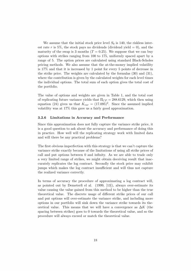
We assume that the initial stock price level S0 is 140, the riskless inter-est rate r is 5%, the stock pays no dividends (dividend yield = 0), and thematurity of the swap is 3 months (T = 0.25). We suppose that we can buyoptions with strikes ranging from 100 to 175, uniformly spaced apart by arange of 5. The option prices are calculated using standard Black-Scholespricing methods. We also assume that the at-the-money implied volatilityis 17% and that it is increased by 1 point for every 5 points of decrease inthe strike price. The weights are calculated by the formulas (30) and (31),where the contribution is given by the calculated weights for each level timesthe individual options. The total sum of each option gives the total cost ofthe portfolio.

The value of options and weights are given in Table 1, and the total costof replicating future variance yields that ΠCP = 288.6129, which then usingequation (24) gives us that Kvar = (17.095)2. Since the assumed impliedvolatility was at 17% this gave us a fairly good approximation.

3.2.6 Limitations in Accuracy and Performance

Since this approximation does not fully capture the variance strike price, itis a good question to ask about the accuracy and performance of doing thisin practice. How well will the replicating strategy work with limited dataand will there be any practical problems?

The first obvious imperfection with this strategy is that we can’t capture thevariance strike exactly because of the limitations of using all strike prices ofcall and put options between 0 and infinity. As we are able to trade onlya very limited range of strikes, we might obtain deceiving result that inac-curately replicates the log contract. Secondly the stock price may exhibitjumps which makes the log contract insufficient and will thus not capturethe realized variance correctly.

In terms of accuracy the procedure of approximating a log contract will,as pointed out by Demeterfi el al. (1999, [13]), always over-estimate itsvalue causing the value gained from this method to be higher than the truetheoretical value. The discrete usage of different strike prices of our calland put options will over-estimate the variance strike, and including moreoptions in our portfolio will sink down the variance strike towards its the-oretical value. This means that we will have a convergence as ∆K (thespacing between strikes) goes to 0 towards the theoretical value, and so theprocedure will always exceed or match the theoretical value.

18

3.3 Volatility Swaps

A volatility swap is a forward contract on future realized volatility. Al-though seemingly very similar to the variance swap, the volatility swap ismore commonly traded in practice but also more theoretically complicated.The Financial Times in 2006 posted an article quoting a derivatives tradersaying [20]:

”Variance is easier to hedge. Volatility can be a nightmare.”

An assets volatility is a good way in measuring riskiness and uncertainty,and thus such a swap will provide a direct exposure to volatility making itan attractive choice. The volatility swap payoff lies close to the varianceswap, and is defined as (√

Vd(0, n, T )−Kvol

)×N (33)

where√Vd(0, n, T ) is the square root of the realized variance, i.e. equation

(1). n is again the number of sampling dates and Kvol is the volatility strike.N refers to the notional amount of the swap.

3.3.1 Example of a Volatility Swap

To get a better feeling of the volatility swap works in practice, we again takea look at a very simple example. Going back with the same variables as inthe variance swap case, we put the notional amount as N = 1,000,000 andwe take a long position in this swap with a volatility strike Kvol of 15%. Atthe end of the contract we find that the realized variance V is calculated tobe 20%. Using again our payoff function we can see that we end with a finalprofit of (0.20− 0.15)× 1, 000, 000 = $50, 000.

3.3.2 Pricing

As in the case of a variance swap, the pricing of a volatility swap starts outquite similarly. We will again define the fair continuous volatility strike assuch as the present value of the contract at time zero is equal to zero. Thiscorresponds to solving the equation

EQ0

[e−rT (

√Vc(0, T )−Kvol)

]= 0. (34)

Thus, as we recall from equation (9) with the variance strike we can expressthe volatility strike price as

Kvol = EQ0

[√Vc (0, T )

]= EQ0

√ 1

T

∫ T

0σ2dt

. (35)

19

In order to get a solution formula we again need to solve the volatility strikeKvol. Since we are dealing with the square root of the variance equationwe can’t use the same replicating strategy as we had in the variance swapsection. A naive approach to solving this problem would be to use the sameprinciple as in the variance swap and just use the square root right away,i.e.

Kvol =√Kvar. (36)

However doing this directly will most likely result in an error since we don’tconsider the convexity notion (or sometimes also known as convexity error)of the square root function. Thus because we are dealing with the squareroot of the variance, we cannot use a model-independent replication ap-proach and thus we have to look for something different. Without havingany specified model we will thus not get any proper formula for Kvol, butwhat we can do however is to create an upper bound with the help of theresults from earlier.

To deal with the convexity of the square root we apply Jensen’s inequality,which says that for a concave square root function we have that E[

√x] ≤√

E[x]. Applying this to the strike prices for both variance and volatilityswaps, we obtain the following upper bound:

Kvol = EQ0 [√Vc(0, T )] ≤

√EQ0 [Vc(0, T )] =

√Kvar. (37)

Hence we can say that the volatility strike is bounded upwards by the squareroot of the variance strike price. This difference is usually called the convex-ity correction. Thus the choice on which model to be used when calculatingthe strike prices, the magnitude of the convexity will be highly dependentupon this choice. One approximation to derive the convexity error is to usea second order Taylor expansion made by Brockhaus and Long (2000, [6]).The result of the calculations is shown below, where the proof is left for thereader in Appendix B:√

Kvar −Kvol ≈V ar[Vc(0, T )]

8√Kvar

3 . (38)

Worth noting is that the convexity correction term is based on the continu-ous realized variance, rather than the discrete one. A discrete version, i.e. afinite number of sampling dates n, will also perform a reasonable good ap-proximation in a model-independent setup (using the replicating approach),as long as n is big enough.

As pointed out by Broadie and Jain (2008, [27]) the convexity correctionformula will not work very well in a Heston stochastic volatility model orMertons jump-diffusion, due to the fact that the Taylor expansion will have

20

higher order terms that are not negligible. Thus in those models this ap-proximation does not provide a good estimate for the fair volatility strikeprice. The error term is these cases will consist of 3rd and 4th order termsas well, making it more complex and perhaps not very suitable for receivinga proper approximation.

3.3.3 Laplace Transforms

An alternative approach in receiving the price of a volatility swap is to makeuse of Laplace transforms. Evaluating a square root function as a Laplacetransformation and using the realized variance we can solve the volatilitystrike price. Introduced by Broadie and Jain (2008, [27]), they proposed ananalytical exact solution using Laplace transforms. They noticed that thesquare root function can be expressed (from the work of Schurger in 2002,[38]) as:

√x =

1

2√π

∫ ∞0

1− e−sx

s32

ds. (39)

Taking expectations on both sides and using Fubini’s theorem we get

E[√x] =

1

2√π

∫ ∞0

1− E[e−sx]

s32

ds. (40)

Changing the x above to the realized variance Vc(0, T ) we thus obtain asolution formula for the volatility strike price. Thus we have that the strikeis given by

Kvol = EQ[√Vc(0, T )] =

1

2√π

∫ ∞0

1− E[e−sVc(0,T )]

s32

ds. (41)

Thus we need to use numerical integration techniques in order to solve theabove integral which yields the volatility strike price.

21

4 Jump Diffusion Model

Up to this point we have considered an approach which only utilizes theclassic Black-Scholes framework, something that is known to have certainunrealistic assumptions. In this section we will focus on the fact that stockreturns do not always behave in the nice continuous way dictated by theGBM, which implicate that they may exhibit jumps. The extension fromthe B-S model would be to implement a model with the presence of jumps.

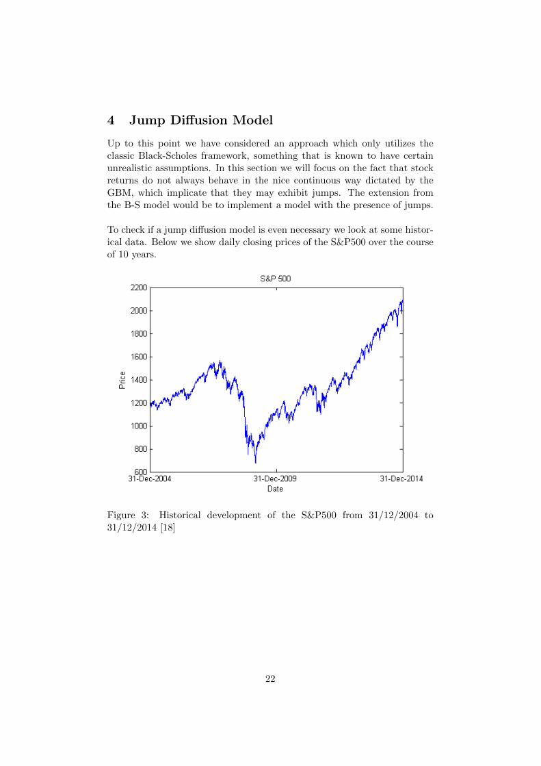
To check if a jump diffusion model is even necessary we look at some histor-ical data. Below we show daily closing prices of the S&P500 over the courseof 10 years.

Figure 3: Historical development of the S&P500 from 31/12/2004 to31/12/2014 [18]

22

As we can see in the market drastic changes occurs from time to time,something that would encourage a jump model. Most notable of this phe-nomenon are in crisis periods, where we can see rapid changes in the price.Although not fully convenient, based on this dataset we can say that theprices in S&P500 tend to experience certain jumps. Whether stock pricesin general really follows a jump process has to be statistically tested andevaluated, and will not be carried out in this thesis. For such a statistic testwe can recommend Stamp and Thorsen (2011, [40]).

Assuming a jump process, there exists a multitude of different models thatuses processes with sudden discrete shifts. It was first proposed that stockprices follow a jump process by John Carrington Cox and Stephen Ross in1976 [12]. They presented a model with a pure jump process such that itworks in discrete time. It was later expanded by Robert Merton to a com-bination of jumps and small continuous movements, and this new process isgenerally known as the Merton Jump Diffusion model (MJD model) [35].

4.1 Jump Dynamics

In a risk-neutral world the dynamics of a jump diffusion model will usuallybe given by

dSt = (r − λm)St−dt+ σSt−dWt + St−dJt. (42)

In a jump model we have a few new parameters in contrast to the originalsetup. J is the added jump process, which will later be defined in equation(43). We have that m is defined as the average jump size, and λ is theintensity of the Poisson process. The subtraction of λm in the risk neutraldrift is done to compensate for the drift related to the jump component. Asthe amount of jumps will be random we need a stochastic counting processand the most common one is a Poisson process, denoted N(t). If we onlyused this process to model the jumps each jump would have unit length soin order to compensate for that we scale it with a random variable. Thisnew process is called a compounded Poisson process and will be a sum ofthe random variables defined as

Jt =

N(t)∑i=1

Ji. (43)

Each term in the sum represents a jump at time 0 < ti < T , with −1 < Jias independent identically distributed random variables. Worth noting isthat the jump direction and jump size will be based on J , which can beeither fixed or random. Although as pointed out in Gatheral (2006, [21]),letting the jump sizes be at a constant value is quite unrealistic. Thereforeit is better in practice to assign a distribution to the jump sizes, and aappropriate and popular fit have shown to be a log-normal distribution.

23

For a more indepth reasoning behind the decision of the distribution werecommend Matsuda (2004, [32]). Thus we will for convenience during thissection assume that J follows a lognormal distribution with mean-jumpparameter a and standard deviation b such that

J ∼ LN(a, b2)⇔ log(J) ∼ N(a, b2). (44)

In a Merton jump-diffusion model the floating leg can be shown to be givenas follows

Vc (0, T ) =1

T

∫ T

0σ2dt+

1

T

N(T )∑i=1

log (Ji)2 . (45)

Applying the same arguments as in earlier sections we can again take theexpected value of the continuous realized variance, and solve the variancestrike price. This yields that assuming a MJD model the continuous strikeprice is given by

Kvar = E[Vc (0, T )] = σ2 + λ(a2 + b2). (46)

One of the great benefits for using the MJD model is that we allow for suddenlarge movements in the spot price, something that has nice implications foroption pricing. The extension from B-S to MJD allows us to add featureswhich tries to capture negative skewness and excess kurtosis of the log stockprice, an area the standard B-S fails to account for.

4.2 The Effect of Jumps

We devote this section to compare the previous approach we had where wepriced a variance swap with as few assumptions as possible, and applyinga replication scheme. We saw that within the Black-Scholes framework wewere able to receive a closed solution formula for the variance strike priceusing a replicating approach. Here we extend the Black-Scholes model, andproceed to look into the same pricing scheme when the dynamics are allowedto exhibit jumps. Thus we will derive the same types of contract as in theprevious chapter, with the added jump feature.

As we are using Ito’s lemma in our derivation without jumps, we will in or-der to compare it effectively with our jump model naturally use Ito’s lemmaagain for a compounded Poisson process. The proof for the calculations isleft for the reader in Appendix A. It follows from the lemma that for anysufficiently smooth function f we have

f (JT )− f (J0) =∑

i≥1,ti≤T

[f(Jt−i

+ JiSt−i

)− f

(Jt−i

)]. (47)

It is important to note that the Poisson jump part of a process and thenormal diffusion part under Ito’s lemma are independent, such that Ito’s

24

lemma for a process which is the sum of a drift-diffusion process and a jumpprocess is just the sum of the Ito’s lemma for the individual parts.

Returning to our specific question we derive the strike price the same wayas we did earlier, with the added change that the stock now follows theequation

St = S0 +

∫ t

0µSsds+

∫ t

0σSsdW +

N(t)∑i=1

JiSt−i. (48)

Our previous approach included both a evaluating a log contract and a stockposition. Thus our next step will be to examine the properties of these twoidentities. Using Ito’s lemma on a log contract with the new stock dynamicswe arrive at

log

(STS0

)=

∫ T

0

(µ− σ2

2

)dt+

∫ T

0σdWt +

N(T )∑i=1

(log(St−i

+ JiSt−i)− log(St−i

)).

(49)

Similarly for the stock position we get

∫ T

0

dStSt

=

∫ T

0µdt+

∫ T

0σdWt +

N(T )∑i=1

(St−i

+ JiSt−iSt−i

−St−iSt−i

). (50)

Combining these equations to arrive at the floating variance leg now adds asum as well as the original functions

∫ T

0

σ2

2dt =

∫ T

0

dStSt− log

STS0−N(T )∑i=1

(Ji − log (1 + Ji)) . (51)

This gives an idea about the error received when a non-jump model is falselyassumed or vice versa. To get a better overview of the effect from each jumpwe consider expanding a log contract as a Taylor expansion such that theinitial term cancel. This gives an error term for each jump with the followingcharacteristics

(Ji − log (1 + Ji)) = Ji − Ji +1

2(Ji)

2 + ... (52)

This leaves us with a dominating term for the error received from each jumpas the square of the jump. This shows that the error on the strike price if ajump free model was assumed. The formula for the variance strike when a

25

jump model is assumed is thus given by the equation

Kjumpvar =

2

TE

[∫ T

0

dStSt−− log

(STS0

)]− 2

TE

N(T )∑i=1

(Ji − log (1 + Ji))

=

2

TE

[∫ T

0

dStSt−− log

(STS0

)]− 2λE [Ji − log (1 + Ji)] .

(53)

This formula is very similar to the formula for the strike price in the casewhen no jumps were assumed although it is important to remember thatthe characteristics of the underlying asset price is different. Although ifcorrectly priced European call and put options exist in the market then thecalculations for hedging the swap with an infinite number of calls and putsare done as in the model without jumps.

Exploring the possibility with a market with infinitely many correctly pricedcall and put options we can approximate the error received by comparing ajump model towards its counterpart with no jumps. As the formula for thestrikes are only slightly different we notice that the extra term is

2λE [Ji − log (1 + Ji)] = λE[J2i + ...

]. (54)

This shows that the approximated error is close to the jump intensity timesthe expected square of the jump size, which gives a linear increase in errorif the intensity changes but a quadratic increase if the jump size increase.

Thus we can see that proceeding with the replication approach when falselyassuming jumps or vice versa can cause quite ineffective results. Deme-terfi et al. (1999, [13]) also points out that neglecting jumps in a syntheticreplication scheme can give substantial errors.

26

5 Stochastic Volatility Models

To measure the dynamics of asset prices or other financial aspects one oftenuses stochastic processes to properly explain the random movements. Usingstochastic processes is a big part of financial mathematics, and has beenknown to play a crucial role in modelling option pricing.

When speaking about random processes and modelling of random move-ments, one of the most famous processes used in the Black-Scholes modelis the geometric Brownian motion (GBM). Empirically it has been shownhowever that the GBM has failed to suffice as a valuable model for pricingand hedging different securities. Looking for better empirical motivation,one idea has been to look towards Levy processes (for an example see Carr,Wu (2004, [9])).

We are however in this chapter going to focus on volatility, and attach-ing a random process on this component. Remember that in the B-S modelwe assume constant volatility, which is something that is generally not truein the market. When it comes to volatility there are quite a few things thatempirically speaks against the Black-Scholes framework. An observationby Mandelbrot (1963, [31]) said that ”large changes tend to be followed bylarge changes, of either sign, and small changes tend to be followed by smallchanges”. This effect is usually known as volatility clustering, and doesn’texist in the B-S model world. Another fallout is the ”leverage effect”, whichsays that decreases in the underlying asset price often results in increasesin volatility. In practice it can also be shown that volatility takes differentvalues depending on moneyness (how much out-of-the-money or in-of-the-money the option is at the current time) as well as term structure. Thisphenomenon is usually called ”volatility smile”, and is a widely debated anddiscussed area in option pricing. To relax the B-S assumption about con-stant volatility in search for better empirical support, stochastic volatilitymodels becomes a natural choice.

After the remarkable introduction of the B-S model in the 70s, there havebeen as pointed out above many debates and arguments about the accu-racy and validity of the solution formulas and the assumptions made in themodel. In search for models to fit the market better, many researches haveturned to stochastic volatility models. These types of models, which nowallows variance to vary in time and be driven by its own process, has beena ground-breaking result in the area of option pricing. Stochastic volatilitymodels can be seen as an extension of Black-Scholes, and tries to capturesome of the flaws in the original model. In this thesis we will focus on the

27

kind of SV models which takes the particular form:

dSt = rStdt+√vtSt

(ρdW 1

t +√

1− ρ2dW 2t

)(55)

dvt = κ (θ − vt) dt+ σvvγt dW

1t . (56)

The first equation (55) gives us the dynamics of the underlying asset: whereSt denotes the asset price at time t, r is the riskless interest rate and

√vt is

the volatility at time t. The two W’s, W 1t and W 2

t , are two standard Brow-nian motions (under the risk neutral measure Q) which allows the diffusionprocesses to be dependent. The correlation between the two is characterizedby the factor ρ. The dynamics of the first equation above will be the samefor the different types of models we will be looking at in this chapter. Worthmentioning is that for simplicity we assume that the asset pays no dividendsand that the interest rate is constant.

The second equation (56) specifies the behaviour of the variance vt as amean-reverting process. The structure for the variance dynamics can bealtered in several ways, for example different types of γ (a free parameterγ > 0) provides different models. The ones we will be looking at in this pa-per will be γ = 1 which corresponds to the GARCH model and γ = 1/2 thefamous Heston model. A slight alteration in the dynamics of the variancealong with γ = 3/2 gives the 3/2 model.

As for the other parameters in the second equation we define θ as the long-run mean variance, κ as the rate of speed in which vt tends to θ, and σv asthe volatility of the volatility, a parameter which will determine the volatilityof the variance process. The type of equation that describes the dynamicsof the variance (56) is generally known as a time-dependent CIR-process(Cox-Ingersroll-Ross process).

5.1 The Heston Model

As mentioned our previous approach in pricing volatility derivatives havebeen to work in a semi model-independent world where no great emphasisor assumptions have been put on the underlying model. In this section welook at the Heston model, a stochastic volatility model which assumes thatthe variance of the asset follows a random process. This model is one ofthe most commonly used when assuming stochastic volatility and was intro-duced by Steven Heston in 1993. [23]

Working with the equations we presented in the beginning of this chap-ter, we now have that γ = 1/2. The Heston model is thus under the riskneutral measure determined by the stochastic process:

dSt = rStdt+√vtSt

(ρdW 1

t +√

1− ρ2dW 2t

)(57)

28

dvt = κ (θ − vt) dt+ σv√vtdW

1t . (58)

The parameters are defined by equation (55) and (56), as well as γ = 1/2.To ensure that the variance process stays positive we restrict that the pa-rameters obey the inequality that 2κθ > σ, a condition known as the Fellercondition (1951, [19]). As usual we denote the index level by S0 as wellas the initial variance process by v0. To obtain the variance process vt, anunobservable process, one has to estimate it from some sort of data (forexample a time series of St).

To price volatility derivatives in this model we already have several pa-rameters to our disposal, which makes us able to calculate the conditionalexpectation of the variance process since it is an ordinary integral equation.The calculations are shown below:

E[vt|v0] = E

[v0 +

∫ t

0κ(θ − vs)ds+

∫ t

0σv√vsdW

1s

∣∣∣∣∣v0]

= E

[v0 +

∫ t

0κ(θ − vs)ds

∣∣∣∣∣v0]

= v0 +

∫ t

0κ(θ − E[vs|v0])ds.

(59)

This integral equation is equivalent to the ordinary differential equationgiven with corresponding initial condition

dE[vt|v0]dt

= κ(θ − E[vt|v0])

E[v0|v0] = v0.(60)

Solving this ODE is a simple task and will, by standard calculations, yielda solution given by

E[vt|v0] = θ + (v0 − θ)e−κt. (61)

When we delve further into the stochastic volatility models this relation willbe of significant importance and have great implications in pricing volatilityderivatives and especially the variance swap.

5.2 The GARCH Model

In a GARCH (Generalized Autoregressive Conditional Heteroskedasticity)model we assume that the stochastic part of the variance process varieswith the variance, compared to the square root of the variance above inthe Heston case. Thus for a standard GARCH(1,1) model we define thefollowing dynamics:

dSt = rStdt+√vtSt

(ρdW 1

t +√

1− ρ2dW 2t

)(62)

29

dvt = κ (θ − vt) dt+ σvvtdW1t . (63)

The various parameters here are defined the same as above, where now γ = 1.Comparing the GARCH model to the Heston model we notice that the onlymathematical difference lies in the dynamics of the variance, but we alsohave in this model that the variance and spot price are uncorrelated. Thismeans that for this model we have that ρ = 0. The GARCH(1,1) model,formulated by Engle and Mezrich (1995, [16]), were given in a discrete settingwhich had the form

log( SnSn−1

)= rn = µ+ un, un = vnεn, εn ∼ N(0, 1) (64)

vn+1 = (1− α− β)V + αu2n + βvn (65)

Here V is the long-run variance, un is the drift-adjusted stock return at timen, α the weight assigned to the squared drift-adjusted return (u2n) and β theweight assigned to the last period variance (vn). This discrete model can betransformed into the continuous time model, where we have the followingparameter relationships:

θ =V

dt(66)

κ =1− α− β

dt(67)

σv = α

√ξ − 1

dt(68)

In the above equation ξ stands for the Pearson kurtosis (fourth moment),calculated from historical data on un. As we stated earlier the GARCH(1,1)model implies an uncorrelation between the spot price and the volatility,something that is certainly not always the case for all models. To approachthe matter one could adopt a Nonlinear GARCH model (NGARCH), whichintroduces an extra term defined as

vn+1 = (1− α− β)V + α(un − c)2 + βvn. (69)

Here we have added an extra parameter, c, which also needs to be estimatedand will facilitate the correlation with the underlying process. We will how-ever not put our focus on this relation here, and the standard GARCH(1,1)will accurately suffice for now. More about the NGARCH process can befound in the original paper by Engle and Ng (1993, [17]).

A considerable difference between the Heston and the GARCH model isthat in this paper we will now utilize historical data in order to estimate fu-ture levels of volatility. This can be seen in contrast to the Heston model inwhich we use option data and market implied estimates of future volatility

30

as calibration tools.

Solving the expected value of the variance we use the same approach aswe had in the Heston model, and after some quick calculations we see thatwe achieve the same result as in the Heston case. With the parameters atour disposal, and considering that the stochastic component vanishes as seenin equation (59), all calculations have already been done. Thus the solutionof the conditional expected value in a GARCH(1,1) model is given by

E[vt|v0] = θ + (v0 − θ)e−κt. (70)

Thus we see that we achieve the same conditional expectation for boththose model, and the only difference lies in the estimation method of theparameters.

5.3 The 3/2 Model

Working in the 3/2 model we can see close similarities with the Heston andGARCH model, but the dynamics of the variance process alter slightly. Oneof the major questions when working with a stochastic volatility model isthe choice of γ, and which value of the parameter would fit reality the best.Bakshi et al. (2006, [2]) estimated in their study a value of approximately1.28 for γ, which suggests that the 3/2 model would be better suited thanthe Heston model which has γ = 0.5.

Following the same setup as earlier, we define the model by the followingdynamics:

dSt = rStdt+√vtSt

(ρdW 1

t +√

1− ρ2dW 2t

)(71)

dvt = κvt (θ − vt) dt+ σvv32t dW

1t . (72)

Again the parameters are defined the same as earlier together with γ = 3/2.The difference here can be seen as having the same dynamics as in theHeston model multiplied by an extra factor of vt, i.e.

dvt = vt[κ (θ − vt) dt+ σv√vtdW

1t ]. [15] (73)

One thing to notice in this model is the interpretation and motivation ofsome of the parameters. The speed of mean reversion (previously κ) willnow be given by the product κ×vt which is now a stochastic quantity. Thiswill imply that the variance will revert more quickly to the mean when itis high. This product then makes the model more suitable to handle fastvolatility increases or decreases, a point at which Heston fails. σv is againthe volatility of volatility, and will for higher values result in heavier tailson the sides. [29]

31

Since the dynamics of the 3/2 models alters in the dynamics of the vari-ance compared to Heston and GARCH, the calculation of the conditionalexpectation becomes slightly different and the quadratic term complicatesthe process. We will however apply the relationship adopted by Drimus(2009, [14]) which gives a link between the 3/2 model and the Heston model.This approach says that the dynamics of 1/vt follows a Heston process withsome specific parameters. Applying Ito’s lemma to 1/vt when vt follows thedynamics of the 3/2 model as in (72) we get

d

(1

vt

)= κθ

(κ+ σ2vκθ

− 1

vt

)dt− σv√

vtdWt. (74)

Thus we notice that the reciprocal of the 3/2 variance process is a Hes-

ton process of parameters(κθ, κ+σ

2v

κθ ,−σv). Having this relationship to our

disposal we can then calculate the conditional expected value for the 3/2model. For simplicity lets denote

κ = κθ (75)

θ =κ+ σ2vκθ

(76)

σv = −σv. (77)

Then our solution for equation (74) is calculated the same way as in (61)with a slight change to the initial condition. Given this solution for E[ 1

vt|v0]

we conclude by inverting back to achieve the final solution which ends upbeing

E [vt| v0] =1

θ +(

1v0− θ)e−κt

. (78)

5.4 Variance Swaps

To derive the price for a variance swap across the different stochastic volatil-ity models we will use the same initial thoughts as in the variance swapsection. In a stochastic volatility model (SV model), we start by definingthe continuous realized variance by

Vc (0, T ) =1

T

∫ T

0vsds. (79)

The fair variance strike price, again denoted by Kvar, defines the value inwhich the contract’s net present value is 0. In terms of equations we have,under the risk neutral measure Q:

EQ0

[e−rT (Vc(0, T )−Kvar)

]= 0. (80)

32

With this we are now able to calculate the continuous realized variancegiven the dynamics we have set up, because we can explicitly calculate theexpected value for the different models. Thus given a SV model, we cansolve this above equation for the variance strike price. In the presence of aGARCH or Heston model, we get the following price:

Kvar = E[Vc(0, T )|v0] = E

[1

T

∫ T

0vtdt

∣∣∣∣∣v0]

=1

T

∫ T

0E[vt|v0]dt =

1

T

∫ T

0

[θ + (v0 − θ)e−κt

]dt

=1

T

(θT +

v0 − θκ

(1− e−κT )).

(81)

Here we notice that the fourth equality comes from the calculation of theconditional expectation, which had been done in equation (59). Thus work-ing within the stochastic volatility models we are able to find an explicitformula for the continuous variance strike price.

In the frame of the 3/2 model, since the conditional expectation of thevariance looks a bit different, we get the following price:

Kvar = E[Vc(0, T )|v0] = E

[1

T

∫ T

0vtdt

∣∣∣∣∣v0]

=1

T

∫ T

0E[vt|v0]dt

=1

T

∫ T

0

1

θ +(

1v0− θ)e−κt

dt

=1

κθTln(v0θ +

(1− v0θ

)e−κT

)+

1

θ.

(82)

Thus given that we can estimate the parameters we are able to obtain theprice of a variance swap with a certain time to maturity T . These calibra-tions and pricing procedures will be done in chapter 6 and 7.

5.5 Volatility Swaps

For the volatility strike however there is no easy way to obtain the strikeprice explicitly, and the only approximations given has been the upper boundthat we saw in the volatility swap section. As we noted earlier, we have toour disposal the convexity correction formula in equation (38). However aspointed out by Broadie and Jain (2008, [27]) the correction formula mightnot be as accurate as one would like in the case of SV models, becausehigher order terms in the Taylor expansion are not negligible. Thus we have

33

fairly limited information of how to properly transition into the volatilityswaps. One thing to solve that would be to allow more terms in the Taylorexpansion for a SV model, but that is a fairly long stretch.

Thus in order to compute the fair volatility strike we will instead in thissection derive a partial differential equation which numerically can be solvedto approximate the volatility strike price. The approach is built on the factof a no-arbitrage relationship between volatility and variance swaps. Wewill also derive a analytical solution for the volatility swap which includesthe use of Laplace transforms and numerical integration, an approach setup by Broadie and Jain (2008, [27]).

5.5.1 PDE Approach

Variance swaps are in their own right very liquid instruments and can beused as a valid trading tool. They can however also be regarded as under-lying assets in order to price other types of volatility instruments includingvolatility swaps and variance options. In this section we derive a PDE toprice volatility derivatives, and in particular give an approximated price ofthe volatility strike price.

Initially we define the price process of the floating leg, denoted by

XTt = EQt

[1

T

∫ T

0vsds

]. (83)

This process is sometimes used as an argument in other price processes thathave a close relation to the floating leg of a variance swap. Since the priceprocess of the floating leg is not completely stochastic because it has, at timet, a deterministic part we will define a state variable It =

∫ t0 vsds to be able

to separate the stochastic and the deterministic part of the process. Thisvariable has a SDE representation of dIt = vtdt. Thus the price process ofthe floating leg has the representation

XTt =

ItT

+ EQt

[1

T

∫ T

tvsds

]. (84)

Then we have for any derivative depending on the floating leg, and in par-ticular the variance swap, a price process G

(t,XT

t

)= F (t, vt, It). Applying

Ito’s lemma on F we get the PDE

dF =∂F

∂tdt+

∂F

∂vdv +

∂F

∂IdI +

1

2

∂2F

∂v2dv2. (85)

Using the above equation (85) we can derive the various PDEs for our dif-ferent SV models.

34

Working with our price process F we thus need to substitute the dynamicsof each model into equation (85). Starting out in the Heston model, theresult can be simplified by collecting terms, arriving at

dF =

[∂F

∂t+∂F

∂vκ (θ − vt) +

∂F

∂Ivt +

1

2

∂2F

∂v2vtσ

2

]dt+

∂F

∂vσ√vtdW

1t . (86)

Since F is a forward price process, its drift under the risk neutral measuremust be zero. Hence solving the PDE for a derivative on the floating leg wecan get an approximation to the price of F:

∂F

∂t+∂F

∂vκ (θ − vt) +

∂F

∂Ivt +

1

2

∂2F

∂v2vtσ

2 = 0. (87)

This above PDE is then solved to compute the fair volatility strike. Theboundary condition needed in order to solve this is

F (T, VT , IT ) =

√ITT

(88)

Thus the framework in which we obtained the PDE in equation (87) canalso be implemented for the other SV models. The results for a GARCHmodel yields the following PDE as well as boundary condition:

∂F

∂t+∂F

∂vκ (θ − vt) +

∂F

∂Ivt +

1

2

∂2F

∂v2v2t σ

2 = 0. (89)

F (T, VT , IT ) =

√ITT

(90)

Substituting the variance dynamics of the 3/2 model into the price processwe get a slightly different PDE, but the mechanics will be done the same asabove. We again have that since F is a price process, the drift under therisk neutral measure has to be zero. Thus we arrive at the PDE

∂F

∂t+∂F

∂vκvt (θ − vt) +

∂F

∂Ivt +

1

2

∂2F

∂v2v3t σ

2 = 0. (91)

F (T, VT , IT ) =

√ITT

(92)

5.5.2 Laplace Transforms

Using the same argument as we did earlier in this, we can numerically solvethe volatility strike price with the use of Laplace Transforms. The continu-ous volatility strike can again be evaluated by the formula defined as

Kvol =1

2√π

∫ ∞0

1− E[e−sVc(0,T )]

s32

ds. (93)

35

Thus in this setting we have to evaluate the expected value in the case ofa Stochastic Volatility model. As an example we look at the Heston modelwhich gives, from Lian (2010, [30]) the following formula:

EQ[e−sVc(0,T )] = exp[A(T, s)−B(T, s)v0] (94)

where

A(T, s) =2κθ

σ2vlog

(2γ(s)e

(γ(s)+κ)T2

(γ(s) + κ)(eγ(s)T − 1) + 2γ(s)

)(95)

B(T, s) =2s(eγ(s)T − 1

T [(γ(s) + κ)(eγ(s)T − 1) + 2γ(s)](96)

γ(s) =

√κ2 + 2

σ2vs

T. (97)

After estimating the parameters we again rely on numerical integration tech-niques in order to solve the integration part in order to obtain the volatilitystrike price.

5.6 Comparison of the Models

As we can see there are some small variations and differences between themodels. Starting off with the variance swap we see that the Heston andGARCH model gives the same explicit formula, where as the 3/2 model be-comes slightly different. For the volatility swaps we received three differentPDEs which can be solved in order to obtain a volatility strike price. Look-ing more into the PDEs we can notice that the variance terms in the secondderivative of the variance alters. For this term we have vt in the Hestonmodel, v2t in the GARCH model and v3t for the 3/2 model. We can also seethat we get an extra vt term in the first derivative of the variance for the3/2 model, due to its extra term in the variance dynamics.

So which model is the optimal one to use? Well we can’t say that yet,and need to estimate the parameters in the models in order to evaluate ourresults. This question also depends on what we are looking for particularly,whether it is accuracy or computational speed, or how the model calculatesdata. All these attributes are all valuable when looking over large datasetsas too complex models may induce heavy computational power.

The most popular out of the three models that we have presented in thissection is undoubtedly the Heston model. It is usually the first model thatcomes to mind when speaking about stochastic volatility models. After sev-eral attempts in extending the Black-Scholes framework, Heston was one ofthe first in creating a model which had the analytical tractability to givesemi-closed form expressions. While GARCH mainly have had its success

36

in econometrics it has over the years found its way into the area of volatilityderivatives, being in close relation to the famous Heston model. It is alsooften estimated using a price-based approach, compared to the others whichare option-based, which will yield different set of parameters when doing theestimations. By Drimus (2009, [14]) the 3/2 model have been shown to givea better empirical support in certain areas, for example supporting upwardsloping implied volatility of variance smiles.

We will later on investigate how well these models perform empirically withestimated parameters. This will be done in chapter 7.

5.7 Stochastic Volatility Models with Jumps

The developments for stochastic volatility models have been revolutionaryin the area of finance in the sense that it gives a more realistic view of howstock prices behave, thus giving a more comprehensive option valuation. Asit stands with most models, there is almost always room for improvements.Generally SV models are good at capturing the volatility smile on longermaturities, but fail to fully support the skew at short maturities as pointedout by Gatheral (2006, [21]). Thus we extend to allow for jumps in thestochastic volatility model, which basically means adding a jump compo-nent to our already existing model.

A model which allows jumps can be divided into two sections, the simplestcase being the Stochastic Volatility with spot Jump model (SVJ model)with jumps in the price process. An extension to the SVJ model is alsoconsidering jumps in the variance process, which we denote as a StochasticVolatility with spot Jump and volatility Jump model (SVJJ). We will thusin this section be looking at both the SVJ and SVJJ model, and give anintroduction into both of these extensions.

5.7.1 Stochastic Volatility with Jumps in the Underlying (SVJ)

The implications for introducing jumps to a SV model will basically look thesame, and we will thus in this section focus our attention on the most famousmodel, the Heston model. If we first allow for jumps in the underlying stockprocess (a so called SVJ model) the risk neutral dynamics then becomes:

dSt = (r − λm)St−dt+√vtSt−

(ρdW 1

t +√

1− ρ2dW 2t

)+ St−dJt (98)

dvt = κ (θ − vt) dt+ σv√vtdW

1t . (99)

The parameters given above are the same as in the Heston model specified in(57) and (58), as well as the applied Merton Jump-Diffusion (MJD) modelwhich is defined in (42). We assume here that the jump process Nt and the

37

Brownian motion are independent.

Calculating the variance strike price in this jump model we apply the sameprocedure as in the regular Heston model, where now we have to into consid-eration the added jump process. Using these results we can then calculatethe price of a variance swap in a SVJ model as

Kvar =1

T

(θT +

v0 − θκ

(1− e−κT ))

+ λ(a2 + b2) [27]. (100)

As we can see the result is fairly straight forward compared to earlier, anddoes not add much complexity. The extra jump process is as we can seeonly added on top of what we already calculated in a Heston model with-out jumps. Thus as long as we know the dynamics for the jumps and theparameters, i.e. λ, a and b, we can receive the price for a variance swapwithout much trouble the same way we did in the original Heston model.The downside to this model is that the jump process is uncorrelated withthe variance process, implicating that that volatility stays the same after ajump occurs in the underlying.

5.7.2 Stochastic Volatility with Jumps in Stock Price and Volatil-ity (SVJJ)

Although adding a jump process to the stochastic volatility models wasconsidered a major improvement, there will always be the quest to findingthe perfect model. Up to this point we have considered a model whichonly contains jumps in the price process, but not allowing for jumps in thevariance process. If we think about this assumption it is quite unrealisticthat the instantaneous volatility would not jump if the stock price jumps.Thus it would be appropriate to apply a SVJJ model, such that we havejumps in both processes. This goes in line with the quote we had earlierabout volatility clustering, that ”large changes tend to be followed by largechanges, of either sign, and small changes tend to be followed by smallchanges”. This model, defined in 1999 by Andrew Matytsin [33], will havethe dynamics given by:

dSt = (r − λm)St−dt+√vtSt−

(ρdW 1

t +√

1− ρ2dW 2t

)+ St−dJ

st (101)

dvt = κ (θ − vt) dt+ σv√vtdW

1t + dJvt . (102)

Added here is a jump process in the dynamics of the variance, namely Jvt .We assume that the jump size in this process are exponential with mean ηJand the correlation between the two jump processes are defined as follows:

Jv ∼ exp

(1

ηJ

), Js|Jv ∼ LN(a+ ρJJ

v, b2). (103)

38

Concluding this section the question to ask now becomes which model ispreferable, the original Heston, the single jump model (SVJ) or the doublejump model (SVJJ). One might assume that including more things and mak-ing a more complex model would fit better, but that is arguably not alwaysthe case. A comparison as a whole for the benefits of adding jumps into themodel is a trade off. Even though we might mitigate some problems that theoriginal model cannot account for (such as short maturity skews), we haveon the other hand increased complexity and in some cases loss of tractability.

Mathematically it becomes more complex when adding jumps, which ofcourse affects the computational speed. As pointed out in Gatheral (2006,[21]), the SVJJ model has more parameters but were also harder to fitobserved option prices. Working with more parameters might be good insome cases, but the main issue with SVJJ is that the added performanceis overmatched by the computational technicality and power needed. TheSVJ model has more parameters than the original Heston model, but as wepointed out the added parameters are technically not that difficult to im-plement, thus giving a better fit to observed data compared to the originalmodel.

5.8 Variance Options

Another interesting derivative in this area is options which are not based onan underlying asset, but instead written on variance or volatility. We willin section derive an approach which introduces variance options. In orderto price variance options, we use a no-arbitrage argument which is similarto the PDE approach we saw in the case of volatility swaps.

Using this strategy we create a specific portfolio which lets us find a partialdifferential equation which will be similar to the ones we saw for the volatil-ity swap. As usual we denote the price of a standard European call optionas:

Ct = EQt [e−r(T−t)max(Vc(0, T )−K, 0)]×N. (104)

We will derive a partial differential equation to price a variance call option,and the payoff of the call can be replicated by continuous trading of a vari-ance swap. This replicating approach will yield the price of the variance calloption. Thus we need to form a portfolio including both a call option and αunits of variance swaps. The created portfolio will at time 0 have a value of

Π0 = α(XT0 −Kvar) + C0. (105)

Worth noting is that the portfolio value will be the same as the variance calloption value because there is no cost to a unit of variance swap at the startof the contract. The price process for the variance call, denoted CTt , can be

39

expressed asCTt = G(t, vt, It) (106)

Applying Ito’s lemma to our price process we get

dG =∂G

∂tdt+

∂G

∂vdv +

∂G

∂IdI +

1

2

∂2G

∂v2dv2. (107)

This equation can be simplified using the parameters from our SV models,and we will perform the calculations in the case of a Heston model. Theprocedures for creating the PDE for variance options are technically donethe same for our different models, and will thus only be carried out in theHeston case. We will only apply this approach in terms of either a GARCH,Heston or 3/2 model, and will in this paper not consider the extensions intothe jump frameworks (SVJ and SVJJ). Putting the variance dynamics fromthe Heston model into G we obtain

dG =

[∂G

∂t+∂G

∂vκ (θ − vt) +

∂G

∂Ivt +

1

2

∂2G

∂v2vtσ

2

]dt+

∂G

∂vσ√vtdW

1t . (108)

From equation (105) the change in portfolio value for a small time step dt is

dΠt = αdF + dG. (109)

Now we notice that we have done both dF (in the volatility swap section)and dG (in this section), which we can use in order to simplify. Thus wesubstitute dF from equation (86) and dG from equation (108) into equation(109) which yields:

dΠt = α(∂F∂v

σv√vtdW

1t

)+[∂G∂t

+∂G

∂vκ(θ − vt) +

∂G

∂Ivt +

1

2

∂2G

∂v2vtσ

2v

]dt

+∂G

∂vσv√vtdW

1t .

(110)

We can now recognize that a suitable choice of α can remove the stochasticcomponent. Thus the random segment vanishes if we choose

α = −∂G∂v

/∂F∂v

. (111)

We can then simplify (110) to

dΠt =[∂G∂t

+∂G

∂vκ(θ − vt) +

∂G

∂Ivt +

1

2

∂2G

∂v2vtσ

2v

]dt. (112)

Noting that the portfolio Πt is riskless, we want it to equal the risk free rateof return (to avoid arbitrage opportunities), which yields[∂G

∂t+∂G

∂vκ(θ − vt) +

∂G

∂Ivt +

1

2

∂2G

∂v2vtσ

2v

]dt = rGdt. (113)

40

This can thus be rewritten as

∂G

∂t+∂G

∂vκ(θ − vt) +

∂G

∂Ivt +

1

2

∂2G

∂v2vtσ

2v − rG = 0. (114)

For the cases of a GARCH or 3/2 model we get slightly different PDEs, whichwill look similarly as in the section of volatility swaps. The correspondingPDEs will be

∂G

∂t+∂G

∂vκ(θ − vt) +

∂G

∂Ivt +

1

2

∂2G

∂v2v2t σ

2v − rG = 0. (115)

∂G

∂t+∂G

∂vκvt(θ − vt) +

∂G

∂Ivt +

1

2

∂2G

∂v2v3t σ

2v − rG = 0. (116)

Solving the partial differential equation (114) in a specific region with properboundary conditions gives the price of a variance call option. These detailswill not be explored in this paper, and more information are given by Broadieand Jain (2008, [26]).

41

6 Parameter Calibrations

Given the different pricing methods and strategies we have introduced so far,we need to estimate the various parameters in order to use them. Thus thischapter will be devoted on calibrating and thereby estimating the parametersfrom our different models. These estimations are based on two differentcalibration techniques, which is either option-based or price-based. Most ofthe models we are looking at will be option-based (which will be the B-S,MJD, Heston and the 3/2 model), and they will be estimated from optiondata from S&P500. The GARCH model is the only model which is price-based, and will be estimated from historical data. For this we will be lookingat the S&P500 index over a historical time period.

6.1 European Options

In order to estimate the parameters from B-S, MJD, Heston or the 3/2model we have gathered European style vanilla options from the S&P500.All options have been collected from the Historical Option Data database,obtained via www.historicaloptiondata.com. The raw dataset consists of 1273 460 European options (both put and calls) on the S&P500. The rangeof the data collected is between 2014-01-01 and 2014-12-31, i.e. one year ofdaily data, which corresponds to 252 trading days of data.

6.1.1 Filtering Process

As we have quite a large dataset it is a good idea before calibration toperform a filtration to eliminate outliers and thus stabilize parameter esti-mation. This will be done to ensure that the estimations are valuable and toobtain efficient and reliable calibrations. There exists a variety of differentfiltration techniques, but we will in this paper apply the filtering schemedone by Bakshi et al. (1997, [3]). Both put and call options can be usedbut it suffices to only concentrate on call options. Thus we start off byeliminating all put options from our dataset. We then proceed to removeall non-traded options, which is done due to illiquidity. We will also removethe options with a time to maturity less than 7 days or greater than 182 days.

Thus in this study we start off with 1 273 460 European S&P500 options.We begin with removing all put options, which consists of 636 730 options.Next we remove the non-traded options due to illiquidity, removing a totalof 524 069 options. In accordance with Bakshi et al. (1997, [3]) we also re-move options that have a time to maturity which is less than 7 days. This isbecause these options are considered illiquid, even though it is worth notingthat these types of options have increased since 1997. Since we are focus-ing on swaps in this thesis, which are usually traded in short maturities,

42

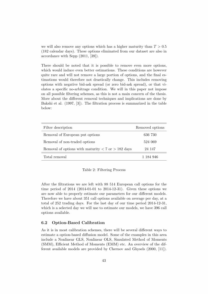
we will also remove any options which has a higher maturity than T > 0.5(182 calendar days). These options eliminated from our dataset are also inaccordance with Sepp (2011, [39]).

There should be noted that it is possible to remove even more options,which would induce even better estimations. These conditions are howeverquite rare and will not remove a large portion of options, and the final es-timations would therefore not drastically change. This includes removingoptions with negative bid-ask spread (or zero bid-ask spread), or that vi-olates a specific no-arbitrage condition. We will in this paper not imposeon all possible filtering schemes, as this is not a main concern of the thesis.More about the different removal techniques and implications are done byBakshi et al. (1997, [3]). The filtration process is summarized in the tablebelow:

Filter description Removed options

Removal of European put options 636 730

Removal of non-traded options 524 069

Removal of options with maturity < 7 or > 182 days 24 147

Total removal 1 184 946

Table 2: Filtering Process

After the filtrations we are left with 88 514 European call options for thetime period of 2014 (2014-01-01 to 2014-12-31). Given these options weare now able to properly estimate our parameters for our different models.Therefore we have about 351 call options available on average per day, at atotal of 252 trading days. For the last day of our time period 2014-12-31,which is a selected day we will use to estimate our models, we have 396 calloptions available.

6.2 Option-Based Calibration

As it is in most calibration schemes, there will be several different ways toestimate a option-based diffusion model. Some of the examples in this areainclude a Nonlinear GLS, Nonlinear OLS, Simulated Method of Moments(SMM), Efficient Method of Moments (EMM) etc. An overview of the dif-ferent available models are provided by Chernov and Ghysels (2000, [11]).

43

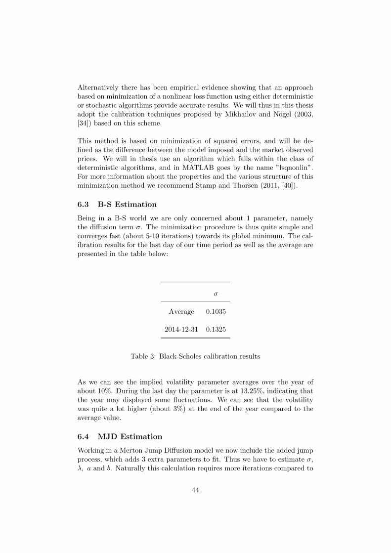
Alternatively there has been empirical evidence showing that an approachbased on minimization of a nonlinear loss function using either deterministicor stochastic algorithms provide accurate results. We will thus in this thesisadopt the calibration techniques proposed by Mikhailov and Nogel (2003,[34]) based on this scheme.

This method is based on minimization of squared errors, and will be de-fined as the difference between the model imposed and the market observedprices. We will in thesis use an algorithm which falls within the class ofdeterministic algorithms, and in MATLAB goes by the name ”lsqnonlin”.For more information about the properties and the various structure of thisminimization method we recommend Stamp and Thorsen (2011, [40]).

6.3 B-S Estimation

Being in a B-S world we are only concerned about 1 parameter, namelythe diffusion term σ. The minimization procedure is thus quite simple andconverges fast (about 5-10 iterations) towards its global minimum. The cal-ibration results for the last day of our time period as well as the average arepresented in the table below:

σ

Average 0.1035

2014-12-31 0.1325

Table 3: Black-Scholes calibration results

As we can see the implied volatility parameter averages over the year ofabout 10%. During the last day the parameter is at 13.25%, indicating thatthe year may displayed some fluctuations. We can see that the volatilitywas quite a lot higher (about 3%) at the end of the year compared to theaverage value.

6.4 MJD Estimation

Working in a Merton Jump Diffusion model we now include the added jumpprocess, which adds 3 extra parameters to fit. Thus we have to estimate σ,λ, a and b. Naturally this calculation requires more iterations compared to

44

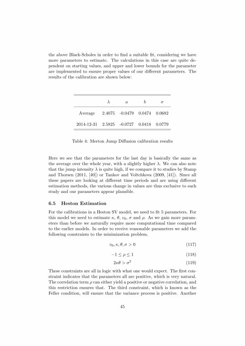
the above Black-Scholes in order to find a suitable fit, considering we havemore parameters to estimate. The calculations in this case are quite de-pendent on starting values, and upper and lower bounds for the parameterare implemented to ensure proper values of our different parameters. Theresults of the calibration are shown below:

λ a b σ

Average 2.4075 -0.0479 0.0474 0.0682

2014-12-31 2.5825 -0.0727 0.0418 0.0779

Table 4: Merton Jump Diffusion calibration results

Here we see that the parameters for the last day is basically the same asthe average over the whole year, with a slightly higher λ. We can also notethat the jump intensity λ is quite high, if we compare it to studies by Stampand Thorsen (2011, [40]) or Tankov and Voltchkova (2009, [41]). Since allthese papers are looking at different time periods and are using differentestimation methods, the various change in values are thus exclusive to eachstudy and our parameters appear plausible.

6.5 Heston Estimation

For the calibrations in a Heston SV model, we need to fit 5 parameters. Forthis model we need to estimate κ, θ, v0, σ and ρ. As we gain more param-eters than before we naturally require more computational time comparedto the earlier models. In order to receive reasonable parameters we add thefollowing constraints to the minimization problem.

v0, κ, θ, σ > 0 (117)

−1 ≤ ρ ≤ 1 (118)

2κθ > σ2 (119)

These constraints are all in logic with what one would expect. The first con-straint indicates that the parameters all are positive, which is very natural.The correlation term ρ can either yield a positive or negative correlation, andthis restriction ensures that. The third constraint, which is known as theFeller condition, will ensure that the variance process is positive. Another

45

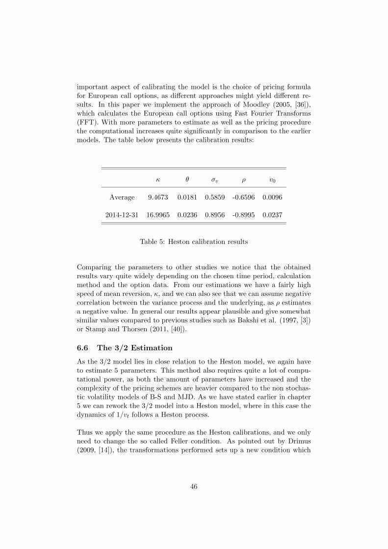
important aspect of calibrating the model is the choice of pricing formulafor European call options, as different approaches might yield different re-sults. In this paper we implement the approach of Moodley (2005, [36]),which calculates the European call options using Fast Fourier Transforms(FFT). With more parameters to estimate as well as the pricing procedurethe computational increases quite significantly in comparison to the earliermodels. The table below presents the calibration results:

κ θ σv ρ v0

Average 9.4673 0.0181 0.5859 -0.6596 0.0096

2014-12-31 16.9965 0.0236 0.8956 -0.8995 0.0237

Table 5: Heston calibration results

Comparing the parameters to other studies we notice that the obtainedresults vary quite widely depending on the chosen time period, calculationmethod and the option data. From our estimations we have a fairly highspeed of mean reversion, κ, and we can also see that we can assume negativecorrelation between the variance process and the underlying, as ρ estimatesa negative value. In general our results appear plausible and give somewhatsimilar values compared to previous studies such as Bakshi et al. (1997, [3])or Stamp and Thorsen (2011, [40]).

6.6 The 3/2 Estimation

As the 3/2 model lies in close relation to the Heston model, we again haveto estimate 5 parameters. This method also requires quite a lot of compu-tational power, as both the amount of parameters have increased and thecomplexity of the pricing schemes are heavier compared to the non stochas-tic volatility models of B-S and MJD. As we have stated earlier in chapter5 we can rework the 3/2 model into a Heston model, where in this case thedynamics of 1/vt follows a Heston process.

Thus we apply the same procedure as the Heston calibrations, and we onlyneed to change the so called Feller condition. As pointed out by Drimus(2009, [14]), the transformations performed sets up a new condition which

46

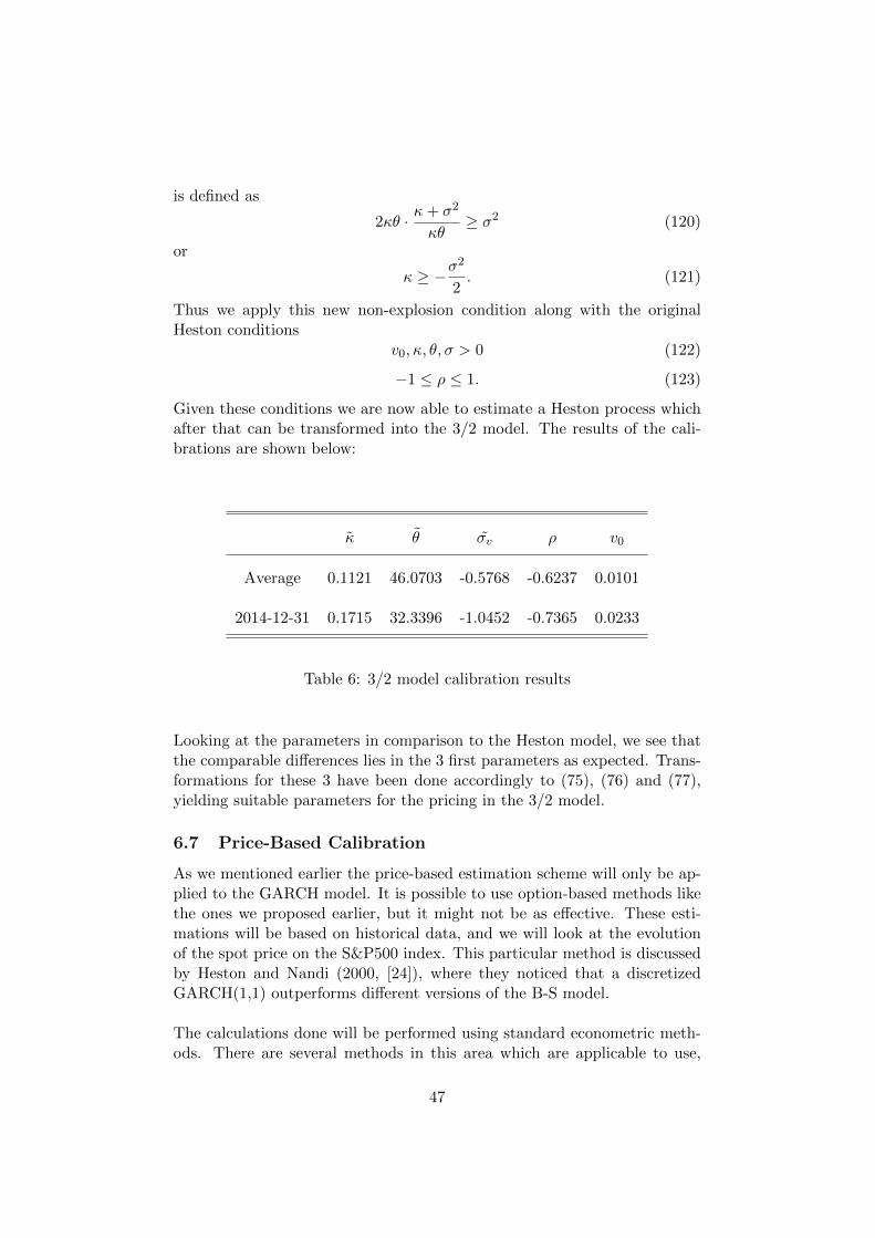
is defined as

2κθ · κ+ σ2

κθ≥ σ2 (120)

or

κ ≥ −σ2

2. (121)

Thus we apply this new non-explosion condition along with the originalHeston conditions

v0, κ, θ, σ > 0 (122)

−1 ≤ ρ ≤ 1. (123)

Given these conditions we are now able to estimate a Heston process whichafter that can be transformed into the 3/2 model. The results of the cali-brations are shown below:

κ θ σv ρ v0

Average 0.1121 46.0703 -0.5768 -0.6237 0.0101

2014-12-31 0.1715 32.3396 -1.0452 -0.7365 0.0233

Table 6: 3/2 model calibration results

Looking at the parameters in comparison to the Heston model, we see thatthe comparable differences lies in the 3 first parameters as expected. Trans-formations for these 3 have been done accordingly to (75), (76) and (77),yielding suitable parameters for the pricing in the 3/2 model.

6.7 Price-Based Calibration

As we mentioned earlier the price-based estimation scheme will only be ap-plied to the GARCH model. It is possible to use option-based methods likethe ones we proposed earlier, but it might not be as effective. These esti-mations will be based on historical data, and we will look at the evolutionof the spot price on the S&P500 index. This particular method is discussedby Heston and Nandi (2000, [24]), where they noticed that a discretizedGARCH(1,1) outperforms different versions of the B-S model.

The calculations done will be performed using standard econometric meth-ods. There are several methods in this area which are applicable to use,

47

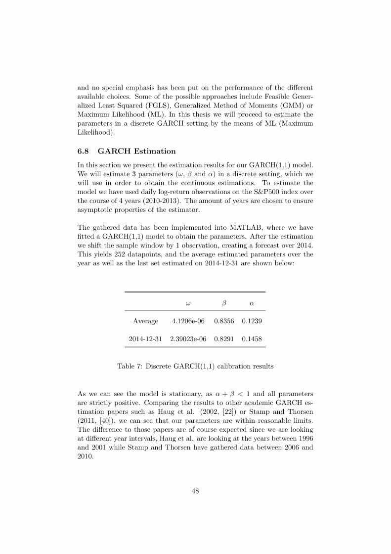
and no special emphasis has been put on the performance of the differentavailable choices. Some of the possible approaches include Feasible Gener-alized Least Squared (FGLS), Generalized Method of Moments (GMM) orMaximum Likelihood (ML). In this thesis we will proceed to estimate theparameters in a discrete GARCH setting by the means of ML (MaximumLikelihood).

6.8 GARCH Estimation

In this section we present the estimation results for our GARCH(1,1) model.We will estimate 3 parameters (ω, β and α) in a discrete setting, which wewill use in order to obtain the continuous estimations. To estimate themodel we have used daily log-return observations on the S&P500 index overthe course of 4 years (2010-2013). The amount of years are chosen to ensureasymptotic properties of the estimator.

The gathered data has been implemented into MATLAB, where we havefitted a GARCH(1,1) model to obtain the parameters. After the estimationwe shift the sample window by 1 observation, creating a forecast over 2014.This yields 252 datapoints, and the average estimated parameters over theyear as well as the last set estimated on 2014-12-31 are shown below:

ω β α

Average 4.1206e-06 0.8356 0.1239

2014-12-31 2.39023e-06 0.8291 0.1458

Table 7: Discrete GARCH(1,1) calibration results

As we can see the model is stationary, as α + β < 1 and all parametersare strictly positive. Comparing the results to other academic GARCH es-timation papers such as Haug et al. (2002, [22]) or Stamp and Thorsen(2011, [40]), we can see that our parameters are within reasonable limits.The difference to those papers are of course expected since we are lookingat different year intervals, Haug et al. are looking at the years between 1996and 2001 while Stamp and Thorsen have gathered data between 2006 and2010.

48

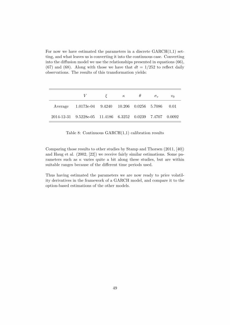
For now we have estimated the parameters in a discrete GARCH(1,1) set-ting, and what leaves us is converting it into the continuous case. Convertinginto the diffusion model we use the relationships presented in equations (66),(67) and (68). Along with those we have that dt = 1/252 to reflect dailyobservations. The results of this transformation yields:

V ξ κ θ σv v0

Average 1.0173e-04 9.4240 10.206 0.0256 5.7086 0.01

2014-12-31 9.5228e-05 11.4186 6.3252 0.0239 7.4707 0.0092

Table 8: Continuous GARCH(1,1) calibration results

Comparing those results to other studies by Stamp and Thorsen (2011, [40])and Haug et al. (2002, [22]) we receive fairly similar estimations. Some pa-rameters such as κ varies quite a bit along these studies, but are withinsuitable ranges because of the different time periods used.

Thus having estimated the parameters we are now ready to price volatil-ity derivatives in the framework of a GARCH model, and compare it to theoption-based estimations of the other models.

49

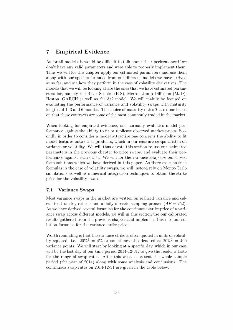
7 Empirical Evidence

As for all models, it would be difficult to talk about their performance if wedon’t have any valid parameters and were able to properly implement them.Thus we will for this chapter apply our estimated parameters and use themalong with our specific formulas from our different models we have arrivedat so far, and see how they perform in the case of volatility derivatives. Themodels that we will be looking at are the ones that we have estimated param-eters for, namely the Black-Scholes (B-S), Merton Jump Diffusion (MJD),Heston, GARCH as well as the 3/2 model. We will mainly be focused onevaluating the performance of variance and volatility swaps with maturitylengths of 1, 3 and 6 months. The choice of maturity dates T are done basedon that these contracts are some of the most commonly traded in the market.

When looking for empirical evidence, one normally evaluates model per-formance against the ability to fit or replicate observed market prices. Sec-ondly in order to consider a model attractive one concerns the ability to fitmodel features onto other products, which in our case are swaps written onvariance or volatility. We will thus devote this section to use our estimatedparameters in the previous chapter to price swaps, and evaluate their per-formance against each other. We will for the variance swap use our closedform solutions which we have derived in this paper. As there exist no suchformulas in the case of volatility swaps, we will instead rely on Monte-Carlosimulations as well as numerical integration techniques to obtain the strikeprice for the volatility swap.

7.1 Variance Swaps

Most variance swaps in the market are written on realized variance and cal-culated from log-returns and a daily discrete sampling process (AF = 252).As we have derived several formulas for the continuous strike price of a vari-ance swap across different models, we will in this section use our calibratedresults gathered from the previous chapter and implement this into our so-lution formulas for the variance strike price.

Worth reminding is that the variance strike is often quoted in units of volatil-ity squared, i.e. 20%2 = 4% or sometimes also denoted as 20%2 = 400variance points. We will start by looking at a specific day, which in our casewill be the last day of our time period 2014-12-31, to give the reader a tastefor the range of swap rates. After this we also present the whole sampleperiod (the year of 2014) along with some analysis and conclusions. Thecontinuous swap rates on 2014-12-31 are given in the table below:

50

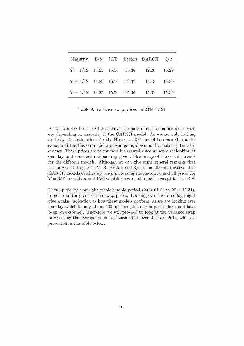
Maturity B-S MJD Heston GARCH 3/2

T = 1/12 13.25 15.56 15.38 12.28 15.27

T = 3/12 13.25 15.56 15.37 14.13 15.30

T = 6/12 13.25 15.56 15.36 15.02 15.34

Table 9: Variance swap prices on 2014-12-31

As we can see from the table above the only model to induce some vari-ety depending on maturity is the GARCH model. As we are only lookingat 1 day, the estimations for the Heston or 3/2 model becomes almost thesame, and the Heston model are even going down as the maturity time in-creases. These prices are of course a bit skewed since we are only looking atone day, and some estimations may give a false image of the certain trendsfor the different models. Although we can give some general remarks thatthe prices are higher in MJD, Heston and 3/2 at smaller maturities. TheGARCH models catches up when increasing the maturity, and all prices forT = 6/12 are all around 15% volatility across all models except for the B-S.

Next up we look over the whole sample period (2014-01-01 to 2014-12-31),to get a better grasp of the swap prices. Looking over just one day mightgive a false indication as how these models perform, as we are looking overone day which is only about 400 options (this day in particular could havebeen an extreme). Therefore we will proceed to look at the variance swapprices using the average estimated parameters over the year 2014, which ispresented in the table below:

51

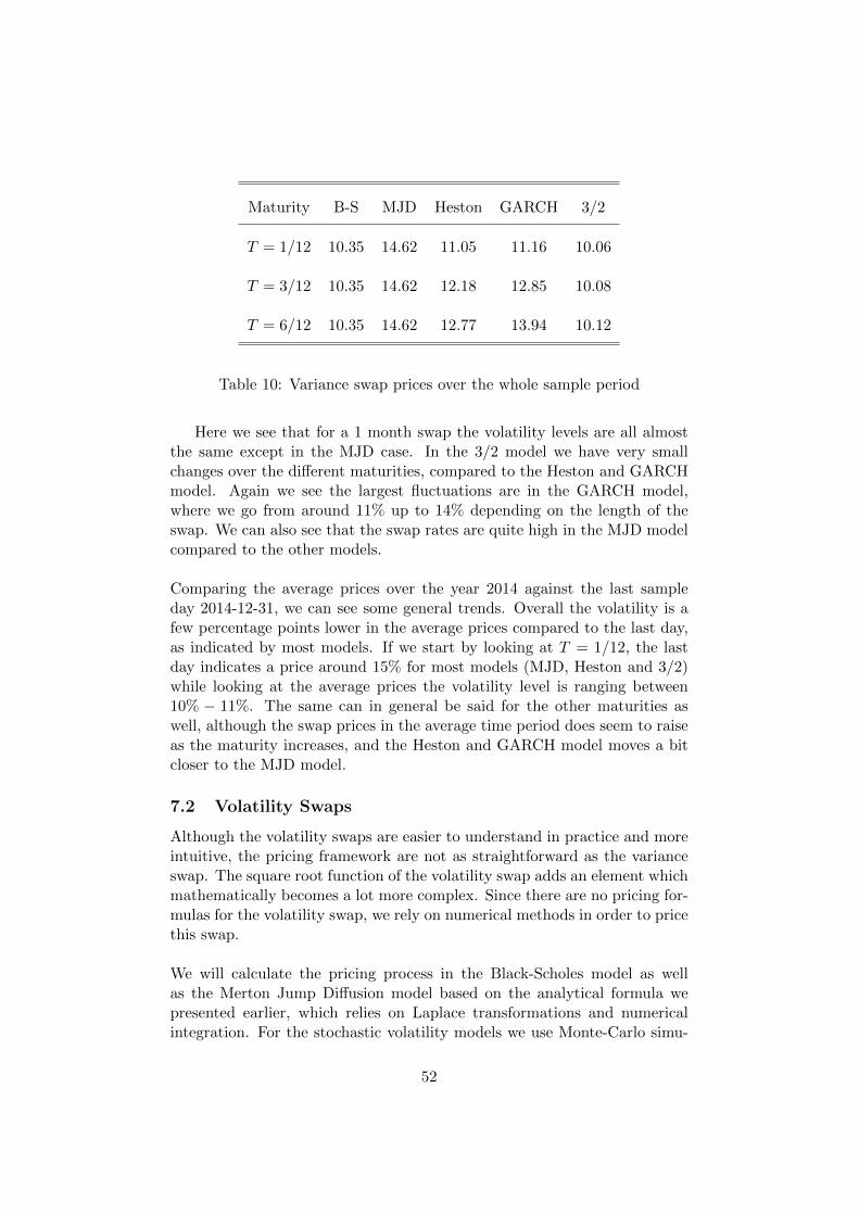
Maturity B-S MJD Heston GARCH 3/2

T = 1/12 10.35 14.62 11.05 11.16 10.06

T = 3/12 10.35 14.62 12.18 12.85 10.08

T = 6/12 10.35 14.62 12.77 13.94 10.12

Table 10: Variance swap prices over the whole sample period

Here we see that for a 1 month swap the volatility levels are all almostthe same except in the MJD case. In the 3/2 model we have very smallchanges over the different maturities, compared to the Heston and GARCHmodel. Again we see the largest fluctuations are in the GARCH model,where we go from around 11% up to 14% depending on the length of theswap. We can also see that the swap rates are quite high in the MJD modelcompared to the other models.

Comparing the average prices over the year 2014 against the last sampleday 2014-12-31, we can see some general trends. Overall the volatility is afew percentage points lower in the average prices compared to the last day,as indicated by most models. If we start by looking at T = 1/12, the lastday indicates a price around 15% for most models (MJD, Heston and 3/2)while looking at the average prices the volatility level is ranging between10% − 11%. The same can in general be said for the other maturities aswell, although the swap prices in the average time period does seem to raiseas the maturity increases, and the Heston and GARCH model moves a bitcloser to the MJD model.

7.2 Volatility Swaps

Although the volatility swaps are easier to understand in practice and moreintuitive, the pricing framework are not as straightforward as the varianceswap. The square root function of the volatility swap adds an element whichmathematically becomes a lot more complex. Since there are no pricing for-mulas for the volatility swap, we rely on numerical methods in order to pricethis swap.

We will calculate the pricing process in the Black-Scholes model as wellas the Merton Jump Diffusion model based on the analytical formula wepresented earlier, which relies on Laplace transformations and numericalintegration. For the stochastic volatility models we use Monte-Carlo simu-

52

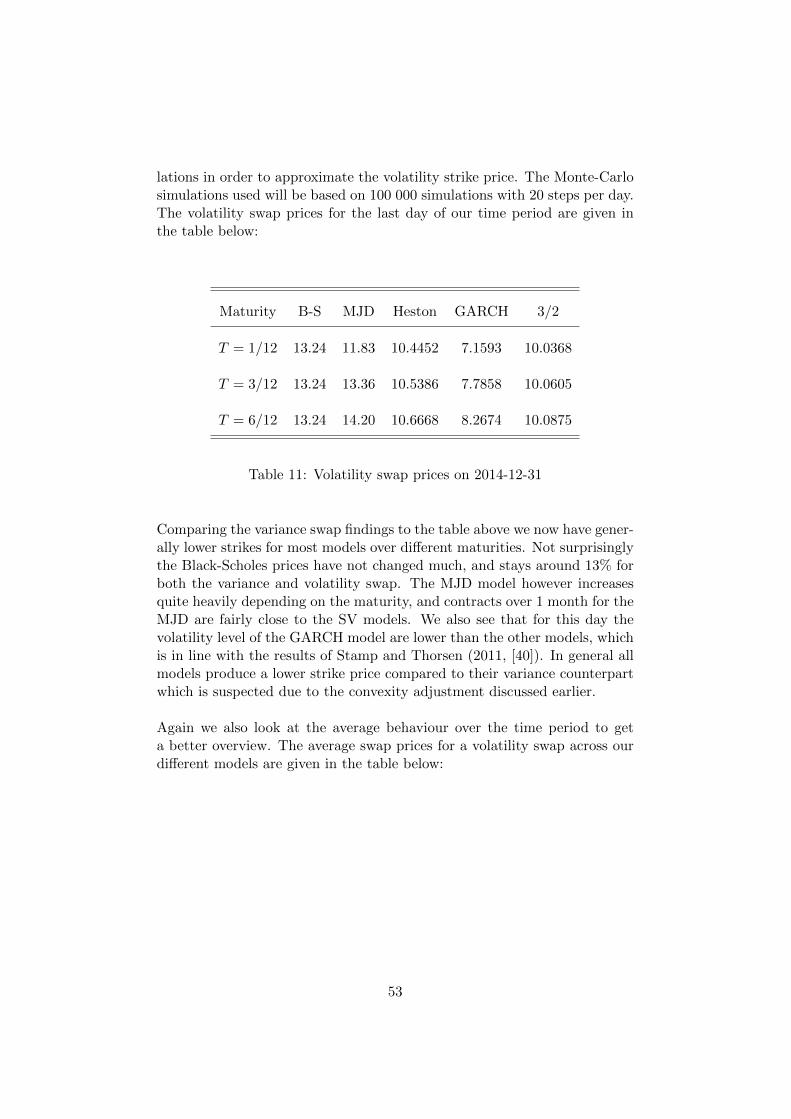
lations in order to approximate the volatility strike price. The Monte-Carlosimulations used will be based on 100 000 simulations with 20 steps per day.The volatility swap prices for the last day of our time period are given inthe table below:

Maturity B-S MJD Heston GARCH 3/2

T = 1/12 13.24 11.83 10.4452 7.1593 10.0368

T = 3/12 13.24 13.36 10.5386 7.7858 10.0605

T = 6/12 13.24 14.20 10.6668 8.2674 10.0875

Table 11: Volatility swap prices on 2014-12-31

Comparing the variance swap findings to the table above we now have gener-ally lower strikes for most models over different maturities. Not surprisinglythe Black-Scholes prices have not changed much, and stays around 13% forboth the variance and volatility swap. The MJD model however increasesquite heavily depending on the maturity, and contracts over 1 month for theMJD are fairly close to the SV models. We also see that for this day thevolatility level of the GARCH model are lower than the other models, whichis in line with the results of Stamp and Thorsen (2011, [40]). In general allmodels produce a lower strike price compared to their variance counterpartwhich is suspected due to the convexity adjustment discussed earlier.

Again we also look at the average behaviour over the time period to geta better overview. The average swap prices for a volatility swap across ourdifferent models are given in the table below:

53

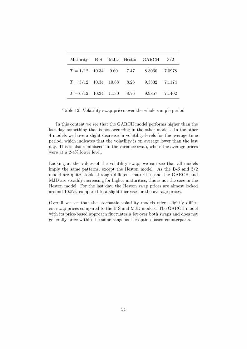
Maturity B-S MJD Heston GARCH 3/2

T = 1/12 10.34 9.60 7.47 8.3060 7.0978

T = 3/12 10.34 10.68 8.26 9.3832 7.1174

T = 6/12 10.34 11.30 8.76 9.9857 7.1402

Table 12: Volatility swap prices over the whole sample period

In this content we see that the GARCH model performs higher than thelast day, something that is not occurring in the other models. In the other4 models we have a slight decrease in volatility levels for the average timeperiod, which indicates that the volatility is on average lower than the lastday. This is also reminiscent in the variance swap, where the average priceswere at a 2-4% lower level.

Looking at the values of the volatility swap, we can see that all modelsimply the same patterns, except the Heston model. As the B-S and 3/2model are quite stable through different maturities and the GARCH andMJD are steadily increasing for higher maturities, this is not the case in theHeston model. For the last day, the Heston swap prices are almost lockedaround 10.5%, compared to a slight increase for the average prices.

Overall we see that the stochastic volatility models offers slightly differ-ent swap prices compared to the B-S and MJD models. The GARCH modelwith its price-based approach fluctuates a lot over both swaps and does notgenerally price within the same range as the option-based counterparts.

54

8 Concluding Remarks

In this thesis we have investigated the field of volatility derivatives, a fi-nancial area that has become quite popular in the recent years. Mainlyfocused on the variance and volatility swap, we have introduced the pricingstrategies for some of the most popular models available as well as given a”model-independent” replicating scheme to price variance swaps which wesaw only requires the use of European call and put options.

To properly evaluate those models we have estimated the various param-eters across our models using either a option-based or price-based approach.For the B-S, MJD, Heston and 3/2 model we gathered European call andput options from the S&P500 during 2014 and applied a squared error min-imization technique to estimate the various parameters. For the price-basedapproach in which the GARCH model was calibrated we used log-returnson the S&P500 index over the course of 4 years (2010-2013), together withthe maximum likelihood calibration technique for the estimations.

Looking over the literature we found that the variance swap was well coveredin terms of analytical formulas and we were able to find closed form solu-tions for our models. As goes for the volatility swap there were limitationsdue to the complexity that the square root function opposes, and no generalsolution formulas could be obtained. Thus we had to rely on numerical in-tegration techniques as well as Monte-Carlo simulations in order to evaluatethe pricing scheme for a volatility swap across all models.

Performance wise we could note that the GARCH model stood out anddid in general not perform exceptionally well. The Heston and 3/2 modelproduced mostly the same patterns depending on the time stamp, and gavea decent performance. The B-S model was typically outside of the range ofthe other models, and was not entirely unexpected fairly underwhelming.The added extension with jumps for the MJD model performed a bit bettercompared to the original Black-Scholes model.

In conclusion it appears that the option-based calibration techniques has asuperior performance. The price-based method which we used for GARCHshowed some flaws in the pricing of swaps, and in general the option-basedcounterpart that has a forward-looking ability in the options seem to prevailover relying on historical data.

55

9 Extensions and Further Research

Our approach in this thesis have been to apply some of the most popularmodels available in the area, as well as putting the ”standard” yet fairlysimple assumptions on the asset. We assumed for instance that the stockpays no dividends, which is in the market usually not the case. Thus ex-tending to allow for cash dividends in the pricing scheme would be a naturalprogress. A study by Klassen (2009, [28]) derives the price for a varianceswap in case of cash dividends, and are using the replication scheme to findthe variance strike price using this extension.

Most of our formulas presented in this thesis are done in a continuous mat-ter, something that is typically not applicable when looking at market data.Although the error between a discrete setting compared to its continuouscounterpart might be low, one should remember that even a 1% error couldimplicate major losses when entering contracts of higher values. Thus a nat-ural extension would be to analyze the different settings against each otherin the framework of volatility derivatives. Both Lian (2010, [30]) as well asBroadie and Jain (2008, [27]) describes the effect of this phenomenon andapplies it to variance and volatility swaps.

Another improvement would be to use stochastic interest rates, since in themarket those rates usually fluctuates over time. Instead of having a regularconstant rate, Horfelt and Torne (2010, [25]) removes the typical constantassumption and presents the value of variance swap in case of stochastic in-terest rates. They look into the case where the interest is driven by its ownIto process, which obviously makes for a more advanced pricing structurewhich may result in reflecting the market better.

Other aspects would be to improve the assumptions about the models, orthe components in them. As we have mentioned earlier, one could exchangethe geometric Brownian motion for a more general Levy process. Carr andLee (2009, [7]) expands the framework and applies a time-changed Levyprocess in order to price variance swaps.

One extension that we touched upon in this thesis was combining the MJDmodel and the stochastic volatility models. Using these two together arequite natural since both the jump aspect and the stochastic volatility imple-mentation are both very reasonable assumptions and have been seen to beempirically viable. Evaluating the SVJ and SVJJ model would make pricingmore realistic and possible better. Stamp and Thorsen (2011, [40]) appliespricing tools for both the variance and volatility swap in the case of the SVJand SVJJ as well as some of the common stochastic volatility models.

56

There are of course even more extensions that can be done to further en-hance the pricing process, as well as other relevant aspects. One of thoseareas include looking at different parameter calibration methods, becauseeven with more advanced models the necessity for reasonable estimation-techniques are equally relevant in the pricing of volatility derivatives.

57

10 Appendix

10.1 A - Compound Poisson Process

We use in the paper Ito’s lemma for a compounded Poisson process and theproof is rather simple. Assumptions include that the process

St =

N(t)∑i=1

Xi (124)

is adapted and that the function f is continuous. To illustrate this factassume that there is only one jump at time tj then

f(St)− f(S0) =(f(St)− f(Stj+ε)

)+(f(Stj+ε)− f(Stj−ε)

)+(f(Stj+ε)− f(S0)

).

(125)

The assumed continuity causes most of the terms to vanish, so that we endup with

f(St)− f(S0) = f(Stj+ε)− f(Stj−ε). (126)

Letting ε go towards zero give us Ito’s lemma for one jump, which can thenbe extended to more jumps by induction with all the paths between thejump vanishing due to continuity.

10.2 B - Brockhaus-Long Convexity Approximation

A proof concerning the convexity error regarding the error between varianceand volatility swaps. We start out by defining a square root function F as:

F (x) =√x. (127)

Calculating the derivatives we know that

F ′(x) =1

2√x

(128)

F ′′(x) = − 1

4√x3 . (129)

Using a Taylor expansion for F around x0 we get

F (x) ≈ F (x0) + F ′(x0)(x− x0) +1

2F ′′(x)(x− x0)2

≈ x1/20 +x− x02√x0− 1

8

(x− x0)2√x0

3

≈ x+ x02√x0− (x− x0)2

8√x0

3 .

(130)

58

Choosing x = V and x0 = E[V ] we get

√V ≈ V + E[V ]

2√E[V ]

− (V − E[V ])2

8√E[V ]

3 . (131)

Finally we take expectations on both sides which yields

E[√V ] ≈ E[V ] + E[V ]

2√E[V ]

− E[(V − E[V ])2]

8√E[V ]

3 (132)

or simplified √E[V ]− E[

√V ] ≈ V ar(V )

8√E[V ]

3 . (133)

Transforming back to our notations in the text we immediately get thatE[√V ] = Kvol as well as

√E[V ] =

√Kvar, which is their respective defini-

tions.

59

References

[1] Applebaum, David Levy Processes - From Probability to Finance andQuantum Groups American Mathematical Society, 2004

[2] Bakshi, G., Ju, N., Yang, H. Estimation of Continuous Time Mod-els With an Application to Equity Volatility Journal of Financial Eco-nomics, 2006

[3] Bakshi, G., Cao, C., Chen, Z. Empirical Performance of AlternativeOption Pricing Models The Journal of Finance, 1997

[4] Black, Fischer & Scholes, Myron The Pricing of Options andCorporate Liabilities Journal of Political Economy, 1973

[5] Breeden, D. & Litzenberger, R. Prices of State-Contingent ClaimsImplicit in Option Prices Journal of Business, October, 1978

[6] Brockhaus, Oliver & Long, Douglas Volatility swaps made sim-ple Risk Magazine, 2000

[7] Carr, Peter & Lee, Roger Pricing Variance Swaps on Time-Changed Levy Processes 2009

[8] Carr, Peter & Lee, Roger Volatility Derivatives Annual Reviewof Financ. Econ., 2009

[9] Carr, Peter & Wu, Liuren Time-Changed Levy Processes andOption Pricing Journal of Financial Economics, 2004

[10] Chicago Board Options Exchange The Volatility Index (VIX)http://www.cboe.com/micro/vix/historical.aspx

[11] Chernov, M. & Ghysels, E Estimation of Stochastic Volatility Mod-els for the Purpose of Option Pricing Computational Finance, 2000

[12] Cox, John C. & Ross, Stephen A. The Valuation of Options forAlternative Stochastic Processes Journal of Financial Economics, 1976

[13] Demeterfi, Kresimir et al. More Than You Ever Wanted To KnowAbout Volatility Swaps March, 1999

[14] Drimus, G. Option on Realized Variance by Transform Methods: Anon-affine Stochastic Volatility Model University of Copenhagen, 2009

[15] Drimus, G. Volatility-of-Volatility Perspectives: Variance Derivativesand Other Equity Exotics University of Copenhagen, 2011

[16] Engle, Robert F & Mezrich, J. Grappling With Garch Risk Mag-azine, 1995

60

[17] Engle, Robert F. & Ng, Victor K. Measuring and Testing theImpact of News on Volatility Journal of Finance, 1993

[18] Finance, Yahoo Daily Closing Prices of S&P500https://finance.yahoo.com/

[19] Feller, W. Two Singular Diffusion Problems Annals of Mathematics,1951

[20] Gangahar, Anuj Volatility Becomes an Asset Class Financial Times,May 2006

[21] Gatheral, Jim The Volatility Surface - A Practitioner’s Guide JohnWiley & Sons, Inc., 2006

[22] Haug, Espen G. et al. GARCH and Volatility Swaps WilmottMagazine, 2002

[23] Heston, S. A Closed-Form Solution for Options with StochasticVolatility with Applications to Bond and Currency Options The re-view of Financial Studies, 1993

[24] Heston, S. & Nandi, S. A Closed-Form GARCH Option ValuationModel The review of Financial Studies, 2000

[25] Horfelt, P. & Torne, O. The Value of a Variance Swap - A Ques-tion of Interest Risk, June 2010

[26] Jain, Ashish & Broadie, Mark Pricing and Hedging VolatilityDerivatives January, 2008

[27] Jain, Ashish & Broadie, Mark The Effect of Jumps and DiscreteSampling on Volatility and Variance Swaps International Journal ofTheoretical and Applied Finance, 2008

[28] Klassen, T. Pricing Variance Swaps with Cash Dividends WilmottJournal, 2009

[29] Koleva, Dessislava Option Pricing under Heston and 3/2 StochasticVolatility Models: an Approximation to the Fast Fourier TransformAarhus University, 2012

[30] Lian, Guanghua Pricing Volatility Derivatives with StochasticVolatility University of Wollongong, 2010

[31] Mandelbrot, Benoit The Variation of Certain Speculative PricesThe Journal of Business, 1963

[32] Matsuda, Kazuhisa Introduction to Merton Jump Diffusion ModelThe City University of New York, 2004

61

[33] Matytsin, Andrew Modelling Volatility and Volatility DerivativesJ.P. Morgan, 1999

[34] Mikhailov, S. & Nogel, U. Heston’s Stochastic Volatility ModelImplementation, Calibration and Some Extensions Wilmott Magazine,2003

[35] Merton, Robert C. Option Pricing When Underlying Stock ReturnsAre Discontinuous Journal of Financial Economics, 1976

[36] Moodley, Nimalin The Heston Model: A Practical Approach withMatlab Code University of the Witwatersrand, 2005

[37] Schultes, Renee Volatility kills market for volatility swaps The WallStreet Journal Europe, 2008

[38] Schurger, Klaus Laplace Transforms and Suprema of StochasticProcesses University of Bonn, 2002

[39] Sepp, Artur Pricing Options on Realized Variance in the Hestonmodel with Jumps in Returns and Volatility - Part II: An ApproximateDistribution of Discrete Variance Journal of Computational Finance,2011

[40] Stamp, Emil S. F. & Thorsen, Thomas F. Pricing of Varianceand Volatility Swaps Aarhus University, 2011

[41] Tankov, P. & Voltchkova, E. Jump-Diffusion Models: A Practi-tioner’s Guide Banque et Marches, 2009

[42] Øksendal, Bernt Stochastic Differential Equations, An Introductionwith Applications Springer-Verlag Berlin Heidelberg, 2010

62