vmc calculations of two-dimensional quantum dots · in this thesis we study systems consisting of...
TRANSCRIPT
VMC CALCULATIONS OFTWO-DIMENSIONAL QUANTUM DOTS
by
LARS EIVIND LERVÅG
THESISfor the degree of
MASTER OF SCIENCE
(Master in Computational Physics)
Faculty of Mathematics and Natural SciencesDepartment of Physics
University of Oslo
November 2010
Det matematisk- naturvitenskapelige fakultetUniversitetet i Oslo


Acknowledgements
First and foremost, my supervisor Morten Hjorth-Jensen is owed a huge thanks. Youhave been a big support during the last two-years, always optimistic, and believing in me;being a source of much inspiration end enthusiasm. Thanks for providing an interestingtopic, and for much advice and good discussions.
My fellow students, Håvard Sandsdalen, Magnus Pedersen Lohne and Sigurd Wenner.Thank you for friendship during the last two years. It is good to have people to talk towhen the work seems endless, and people to discuss problems with.
My family should also be thanked. My mother and father, for believing in me andsupporting me. Thanks to my brother Karl Yngve Lervåg for a lot of help with proof-reading this thesis. I would also like to thank my brothers Alf and Karl Yngve Lervågfor help with emacs and LaTeX, and my brother Jon Vegard Lervåg and his wife StineWalderhaug for continuous support.
In addition, I have had some help with object orienting the code, as I did not haveany previous knowledge of this in C++. My thanks go out to Kyrre Ness Sjøbæk.
Lars Eivind Lervåg


Contents
1 Introduction 9
I Theory 11
2 Quantum Mechanics 132.1 Historical overview . . . . . . . . . . . . . . . . . . . . . . . . . . . . . . . 13
2.1.1 Planck’s law of radiation . . . . . . . . . . . . . . . . . . . . . . . . 142.1.2 The photoelectric effect . . . . . . . . . . . . . . . . . . . . . . . . 15
2.2 Bra-Ket notation . . . . . . . . . . . . . . . . . . . . . . . . . . . . . . . . 162.3 The fundamental postulates of quantum mechanics . . . . . . . . . . . . . 16
2.3.1 Postulate 1 . . . . . . . . . . . . . . . . . . . . . . . . . . . . . . . 162.3.2 Postulate 2 . . . . . . . . . . . . . . . . . . . . . . . . . . . . . . . 172.3.3 Postulate 3 . . . . . . . . . . . . . . . . . . . . . . . . . . . . . . . 182.3.4 Postulate 4 . . . . . . . . . . . . . . . . . . . . . . . . . . . . . . . 192.3.5 Postulate 5 . . . . . . . . . . . . . . . . . . . . . . . . . . . . . . . 19
2.4 Quantum Mechanics in the Schrödinger Picture . . . . . . . . . . . . . . . 202.5 Singe-Particle Quantum Mechanics . . . . . . . . . . . . . . . . . . . . . . 21
2.5.1 Spin . . . . . . . . . . . . . . . . . . . . . . . . . . . . . . . . . . . 222.5.2 Total single-particle wave function . . . . . . . . . . . . . . . . . . 24
2.6 The particle in a box . . . . . . . . . . . . . . . . . . . . . . . . . . . . . . 25
3 Many-Body Theory 293.1 The Many-Body Problem . . . . . . . . . . . . . . . . . . . . . . . . . . . 293.2 Identical particles . . . . . . . . . . . . . . . . . . . . . . . . . . . . . . . . 313.3 The Non-Interacting System . . . . . . . . . . . . . . . . . . . . . . . . . . 34
3.3.1 The ground state of the non-interacting system . . . . . . . . . . . 353.4 The Interacting System . . . . . . . . . . . . . . . . . . . . . . . . . . . . 36
4 Quantum Dots - The Artificial Atoms 374.1 Semiconductors and quantum dots . . . . . . . . . . . . . . . . . . . . . . 384.2 Electrical properties resulting from quantum confinement . . . . . . . . . 404.3 Optical properties resulting from quantum confinement . . . . . . . . . . . 414.4 Applications of quantum dots . . . . . . . . . . . . . . . . . . . . . . . . . 43
5 Theoretical approximations to quantum dots in two dimensions 475.1 One-electron quantum dot . . . . . . . . . . . . . . . . . . . . . . . . . . . 485.2 Two-electron quantum dot . . . . . . . . . . . . . . . . . . . . . . . . . . . 555.3 The N -electron Hamiltonian . . . . . . . . . . . . . . . . . . . . . . . . . . 59

CONTENTS
5.4 Scaling the N -electron Hamiltonian . . . . . . . . . . . . . . . . . . . . . . 60
6 Quantum Monte Carlo 616.1 Random numbers . . . . . . . . . . . . . . . . . . . . . . . . . . . . . . . . 62
6.1.1 Generation of uniform random numbers . . . . . . . . . . . . . . . 636.1.2 Generation of Gaussian distributed random number . . . . . . . . 63
6.2 Monte Carlo integration . . . . . . . . . . . . . . . . . . . . . . . . . . . . 636.2.1 Importance sampling . . . . . . . . . . . . . . . . . . . . . . . . . . 65
6.3 Markov chains and the Metropolis-Hastings algorithm . . . . . . . . . . . 666.4 The variational principle . . . . . . . . . . . . . . . . . . . . . . . . . . . . 696.5 The quantum variational Monte Carlo method (QVMC) . . . . . . . . . . 71
6.5.1 Calculating the energy and variance of our system . . . . . . . . . 716.5.2 Simple Metropolis sampling . . . . . . . . . . . . . . . . . . . . . . 736.5.3 Generalized Metropolis sampling . . . . . . . . . . . . . . . . . . . 73
6.6 Energy minimization using DFP . . . . . . . . . . . . . . . . . . . . . . . 766.7 Blocking . . . . . . . . . . . . . . . . . . . . . . . . . . . . . . . . . . . . . 786.8 Time-step extrapolation . . . . . . . . . . . . . . . . . . . . . . . . . . . . 79
7 The trial wave function 817.1 Slater determinants . . . . . . . . . . . . . . . . . . . . . . . . . . . . . . . 81
7.1.1 Splitting up our Slater determinant . . . . . . . . . . . . . . . . . . 837.1.2 Single-particle orbitals . . . . . . . . . . . . . . . . . . . . . . . . . 847.1.3 Derivatives of the single-particle orbitals . . . . . . . . . . . . . . . 84
7.2 The Jastrow function . . . . . . . . . . . . . . . . . . . . . . . . . . . . . . 867.2.1 Cusp conditions . . . . . . . . . . . . . . . . . . . . . . . . . . . . . 87
7.3 The total trial wave function . . . . . . . . . . . . . . . . . . . . . . . . . 89
II Implementation and results 91
8 Implementation of the QVMC method 938.1 Optimizing the calculations . . . . . . . . . . . . . . . . . . . . . . . . . . 93
8.1.1 The RD-ratio . . . . . . . . . . . . . . . . . . . . . . . . . . . . . . 958.1.2 The RJ -ratio . . . . . . . . . . . . . . . . . . . . . . . . . . . . . . 978.1.3 The GD-ratio . . . . . . . . . . . . . . . . . . . . . . . . . . . . . . 988.1.4 The GJ -ratio . . . . . . . . . . . . . . . . . . . . . . . . . . . . . . 998.1.5 The LD-ratio . . . . . . . . . . . . . . . . . . . . . . . . . . . . . . 1008.1.6 The LJ -ratio . . . . . . . . . . . . . . . . . . . . . . . . . . . . . . 101
8.2 Class implementation . . . . . . . . . . . . . . . . . . . . . . . . . . . . . . 1028.2.1 The initialization of the program . . . . . . . . . . . . . . . . . . . 1028.2.2 Implementation of the Metropolis-Hastings algorithm . . . . . . . . 107
8.3 Parallel computing . . . . . . . . . . . . . . . . . . . . . . . . . . . . . . . 1128.4 Implementing the DFP algorithm . . . . . . . . . . . . . . . . . . . . . . . 1138.5 Implementation of blocking . . . . . . . . . . . . . . . . . . . . . . . . . . 1148.6 Implementation of time-step extrapolation . . . . . . . . . . . . . . . . . . 116
6

CONTENTS
9 Computational results 1179.1 Validating the code . . . . . . . . . . . . . . . . . . . . . . . . . . . . . . . 117
9.1.1 The non-interacting system . . . . . . . . . . . . . . . . . . . . . . 1179.1.2 The two-particle case . . . . . . . . . . . . . . . . . . . . . . . . . . 118
9.2 Variational plots — Finding the optimal parameters . . . . . . . . . . . . 1229.2.1 Simulation of a six-electron quantum dot . . . . . . . . . . . . . . . 1229.2.2 Simulation of a twelve-electron quantum dot . . . . . . . . . . . . . 1229.2.3 Simulation of a twenty-electron quantum dot . . . . . . . . . . . . 1249.2.4 Minimization with DFP . . . . . . . . . . . . . . . . . . . . . . . . 124
9.3 Time-step analysis with blocking . . . . . . . . . . . . . . . . . . . . . . . 1279.3.1 Two electrons . . . . . . . . . . . . . . . . . . . . . . . . . . . . . . 1279.3.2 Six electrons . . . . . . . . . . . . . . . . . . . . . . . . . . . . . . 1279.3.3 Twelve electrons . . . . . . . . . . . . . . . . . . . . . . . . . . . . 1299.3.4 Twenty electrons . . . . . . . . . . . . . . . . . . . . . . . . . . . . 130
9.4 Changing the oscillator frequency . . . . . . . . . . . . . . . . . . . . . . . 1309.5 Splitting up the energy . . . . . . . . . . . . . . . . . . . . . . . . . . . . . 1309.6 Discussions of the results . . . . . . . . . . . . . . . . . . . . . . . . . . . . 1329.7 Quantum dots with more than twenty electrons . . . . . . . . . . . . . . . 134
10 Conclusion 137
A Statistics 141
Bibliography 149
7


Chapter 1
Introduction
In this thesis we study systems consisting of several interacting electrons. More spe-cific, we study systems named quantum dots. Quantum dots are in the literature oftendubbed artificial atoms, due to their many similarities with atoms, even though they donot have a nucleus. Quantum dots are of interest because of their many applications inmodern technology. Furthermore they are fundamentally interesting because they allowus to study electronic systems without the presence of a nucleus that affects the electrons.Moreover, they allow us to easily study effects of quantum confinement. We will give alonger introduction and motivation of quantum dots in Chapter 4.
The aim of this thesis is to do numerical studies of closed-shell quantum dots, usingthe Quantum Variational Monte Carlo (QVMC) ab initio method (See Chapter 5 and 6for details). We consider the so-called parabolic (or circular) quantum dot in two dimen-sions. An object of essential importance for the QVMC method is the trial wave function.This will be our guess at how the functional form of the true many-body wave functionlooks like. In order to construct a good trial wave function, we need to understand thephysics that govern the system of interest. In this thesis we use a Jastrow-Slater wavefunction (see Chapter 7 for details). We want to see if a trial wave function with onlyone Slater determinant (see Chapter 3) is a good approximation for a closed-shell system.We aim to develop a code that can do computations on closed-shell quantum dots withmore than twenty electrons. As far as we know, there has not been done any ab initiocalculations on systems with this many particles.
Another aim is to develop a good QVMC machinery for studying electronic systems.We will not actually do calculations for other systems in this work, but we know thatwhen the code works for the quantum dot system, it can easily be changed to work foratomic or molecular systems.
Overview
The thesis is structured into two main parts. In the first part we present the theoreticalfoundation of this thesis. We have organized this into six chapters:
• Chapter 2 gives a short review of non-relativistic quantum mechanics, including thefundamental postulates of the theory. We will focus on single-particle theory, andgive a short example of a quantum mechanical system; the infinite square well.

Chapter 1. Introduction
• In Chapter 3 we will present non-relativistic many-body theory; quantum mechan-ics for systems consisting of more than one particle. We will present the insolvablemany-body problem. Then we discuss the basic properties a fermionic wave func-tion must exhibit. We will solve the non-interacting system, which introduces theimportant concept of Slater determinants. We will briefly discuss the interactingsystem.
• Chapter 4 gives a presentation of quantum dots; what they are, and why we likethem. We will present some theory of semiconductors and quantum dots such aselectronic band structure and excitations. We will then briefly go through some ofthe interesting applications of quantum dots.
• In Chapter 5 we solve the one-particle problem related to the parabolic quantumdot. This is of importance when we construct the Slater determinant of the trialwave function. We will also solve the two-particle problem for a specific case. Wethen construct the many-particle Hamiltonian and scale it to a dimensionless form.
• Chapter 6 presents the theory of quantum variational Monte Carlo (QVMC) meth-ods. We first discuss random numbers and pseudo-random numbers. We then dis-cuss the basic idea behind Monte-Carlo integration and importance sampling. Wewill discuss the theory of Markov chains which leads us to the important Metropolis-Hastings algorithm. We then present the variational principle. This principle iswhat actually enables us to do QVMC in the first place. We are then ready todiscuss the QVMC method. Finally we will discuss some methods used to improvethe results: The Davidon-Fletcher-Powell (DFP) algorithm, blocking and time-stepextrapolation (see sections 6.6 - 6.8).
• Chapter 7 deals with constructing our trial wave function. We will construct ourSlater determinant out of the single-particle orbitals from Chapter 5. We then dis-cuss the correlation function used in this thesis, the Pade-Jastrow function. Finally,we give the functional form of our trial wave function.
In the second part of this thesis, we explain the implementation of the QVMC method,and present our numerical results. This part is organized in three chapters:
• In Chapter 8 we present the structure of the code developed in this thesis. We havedeveloped an entire QVMC machinery for solving closed-shell parabolic quantumdot systems. We will explain in detail how the QVMC algorithm is implemented.We also go through the implementation of the DFP, blocking and time-step extrap-olation techniques.
• In Chapter 9 we present our results. We will mostly consider parabolic quantumdots with two, six, twelve and twenty particles. The results are discussed andanalyzed. We will also present results for 30 and 42 electrons.
• In Chapter 10 we conclude the thesis.
10

Part I
Theory

Chapter 2
Quantum Mechanics
Mechanics is the field of physics concerned with the behaviour of physical bodies underthe influence of forces, and how these bodies affect their environment. There are twomajor sub-fields: Classical mechanics and quantum mechanics. The first field is used fordescribing the dynamics of macroscopic objects. The second field is used for describingthe dynamics of microscopic objects.
It is assumed that the reader of this thesis is well acquainted with the fundamentalsof quantum physics. Even so, we feel it is important to give a quick review of the basicaspects of the theory in order to clarify some of the notation and to help freshen up thereader’s memory.
Put simply, quantum mechanics is a theoretical framework which has been able todescribe, correlate and predict the behaviour of a vast number of physical systems. Inthis chapter, we first give a short historical overview explaining why quantum mechanicswas needed. We then move on to describe some of the quantum mechanical formalism.We will go through the fundamental postulates of quantum mechanics, and give a briefexplanation to each of them. We then move on to the formalism of quantum mechanicsin the Schrödinger picture, and go through the basic aspects of quantum mechanics fora single-particle system. We conclude with discussing and solving the particle in a box,a famous and fundamental problem in quantum mechanics. If the reader is in need of adeeper introduction to the field, we refer to [1, 2].
2.1 Historical overview
The theoretical description of Nature called quantum mechanics was created by Europeanphysicists in the early 20th century. It was an intellectual revolution that introducedseveral concepts that had been totally unknown in the classical theory of physics:
• Quantization: Many physical quantities can only take certain discrete values.
• Wave-particle dualism: A material particle and electromagnetic radiation is notas different as in classical physics. They both show particle- and wave-like proper-ties.
• Probability interpretation: The quantum mechanical description can only givethe probability for finding a particle at a certain place.
Chapter 2. Quantum Mechanics
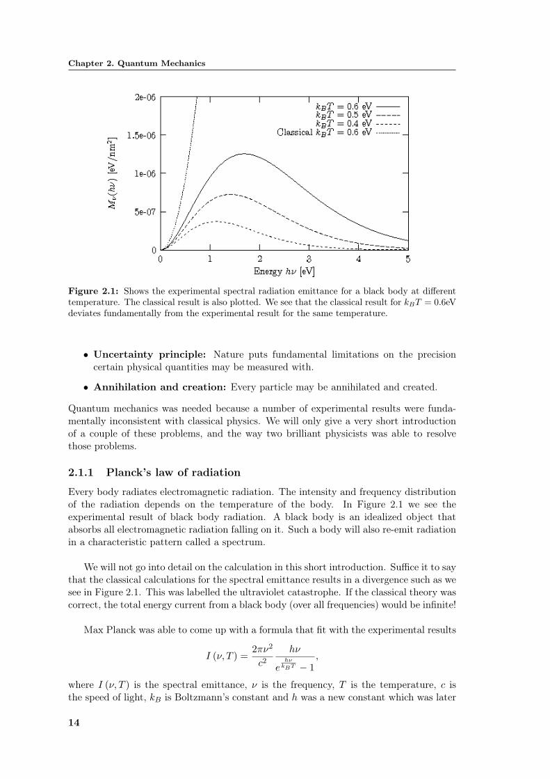
Figure 2.1: Shows the experimental spectral radiation emittance for a black body at differenttemperature. The classical result is also plotted. We see that the classical result for kBT = 0.6eVdeviates fundamentally from the experimental result for the same temperature.
• Uncertainty principle: Nature puts fundamental limitations on the precisioncertain physical quantities may be measured with.
• Annihilation and creation: Every particle may be annihilated and created.
Quantum mechanics was needed because a number of experimental results were funda-mentally inconsistent with classical physics. We will only give a very short introductionof a couple of these problems, and the way two brilliant physicists was able to resolvethose problems.
2.1.1 Planck’s law of radiation
Every body radiates electromagnetic radiation. The intensity and frequency distributionof the radiation depends on the temperature of the body. In Figure 2.1 we see theexperimental result of black body radiation. A black body is an idealized object thatabsorbs all electromagnetic radiation falling on it. Such a body will also re-emit radiationin a characteristic pattern called a spectrum.
We will not go into detail on the calculation in this short introduction. Suffice it to saythat the classical calculations for the spectral emittance results in a divergence such as wesee in Figure 2.1. This was labelled the ultraviolet catastrophe. If the classical theory wascorrect, the total energy current from a black body (over all frequencies) would be infinite!
Max Planck was able to come up with a formula that fit with the experimental results
I (ν, T ) =2πν2
c2hν
ehν
kBT − 1,
where I (ν, T ) is the spectral emittance, ν is the frequency, T is the temperature, c isthe speed of light, kB is Boltzmann’s constant and h was a new constant which was later
14

2.1. Historical overview
named Planck’s constant. The new constant had to be about 6.6 · 10−34Js to get agree-ment with the data.
Planck was able to later explain this empirical formula by assuming that the energyfor radiation with frequency ν was quantized in units hν, i. e. only taking discrete values
E = 0, hν, 2hν, 3hν, ...
This energy quantizing was a totally new idea, and it marked the beginning of quantumphysics.
Planck himself never fully accepted that this was a revolutionary idea. To him itwas only “an act of desperation.” Even so, Planck received the Nobel prize in 1918 for“introducing the quantum” as a real physical entity.
2.1.2 The photoelectric effect
The photoelectric effect is a phenomenon in which electrons are emitted from matter asa consequence of their absorption of energy from electromagnetic radiation. It was firstobserved by Heinrich Hertz in 1887. Experiments showed that if the frequency was belowa certain limit ν0, no electrons would be emitted. Experiments also showed that thekinetic energy of the electrons that were emitted was independent of the intensity of theradiation, but varied linearly with the frequency of the radiation:
Ekin = h (ν − ν0) , ν > ν0.
That electrons may be emitted from matter by electromagnetic radiation was under-standable in the classical theory. But in the classical theory energy is proportional tothe intensity of the radiation. The frequency dependency was therefore baffling for thephysicists in the 19th century.
Albert Einstein solved the problem by assuming that light consists of discrete quanta,photons, with energy
E = hν,
determined by the frequency. When an electron absorbs a photon, the energy of theelectron increases by hν. Some of this energy, W , is needed to liberate the electron fromthe matter, and the rest is just converted to kinetic energy:
Ekin = hν −W.
This is consistent with experiments: The kinetic energy of the electrons varies linearly,with a cutoff frequency ν0 = W/h.
There were several other problems which classical physics could not resolve, like theCompton-effect, diffraction of electrons and the heat capacity of a diatomic gas. A deeperdiscussion of these topics can be found in ref. [1].
From the two cases discussed above, we see that some of the problems that classicalphysics could not explain was resolved by “introducing the quantum.” This was, of course,why the new physical theory was labelled quantum physics.
15
Chapter 2. Quantum Mechanics
2.2 Bra-Ket notation
To make the notation more concise, we introduce some standard notation. Integrals oftentake up a lot of space in formulas, and as they are very much used in quantum mechanicsthrough expressions for expectation values, it is very useful to introduce a compact wayto write such integrals. Say we have a state Ψ. This state can be expressed through thestate vector |Ψ〉, also called a ket. The dual state (complex conjugate) is then representedby 〈Ψ|, called a bra.
We now define the expectation value of an operator O through
ˆ〈O〉 =∫
Ψ∗OΨdx (2.1)
≡ 〈Ψ|OΨ〉. (2.2)
For an arbitrary operator we have that
〈Ψ|OΨ〉 = 〈O†Ψ|Ψ〉 ≡ 〈Ψ|O|Ψ〉, (2.3)
where the dagger meansO† ≡ O∗T , (2.4)
i. e. the operators Hermitian conjugate. The standard notation in quantum mechanicsfor the expectation value is then
ˆ〈O〉 = 〈Ψ|O|Ψ〉. (2.5)
2.3 The fundamental postulates of quantum mechanics
Every fundamental physical theory is based on a set of postulates, quantum mechanicsbeing no exception. In this section we present the postulates of quantum mechanics, andgive a brief explanations on each of them.
Note that different learning books on the subject presents the postulates in differentorder, and with different phrasing. In the following we follow closely the text of ref. [2].
2.3.1 Postulate 1
The physical state Ψ of an isolated quantum mechanical system is represented by a vector|Ψ〉 in a Hilbert space.
Notes on postulate 1: A Hilbert space, H, is a complex vector space with an in-ner product. It is also complete. In the bra-ket formalism, for every quantum state |Ψ〉 ina Hilbert space, there exists a dual state 〈Ψ| in a dual vector space. An inner product isa structure which associates each pair of vectors in the space with a scalar quantity calledthe inner product of the vectors. In the bra-ket formalism we denote the inner product.
〈α|β〉. (2.6)
It satisfies the following three axioms for all vectors |α〉 , |β〉 , |ν〉 ∈ H and all scalars c ∈ C:Conjugate symmetry:
〈α|β〉 = 〈α|β〉∗. (2.7)
16

2.3. The fundamental postulates of quantum mechanics
Linearity in the right argument:
〈α|cβ〉 = c〈α|β〉 (2.8)〈α|β + ν〉 = 〈α|β〉+ 〈α|ν〉. (2.9)
Positive definiteness:〈α|α〉 ≥ 0. (2.10)
For more details into linear algebra, we refer to [3].
Assume we have a discrete basis which is orthonormal
〈i|j〉 = δmn, (2.11)
and complete ∑i
|i〉 〈i| = 1, (2.12)
with δmn being the Kronecker delta, and 1 the identity operator. The quantum state canthen be developed in this basis
|ψ〉 =∑
i
|i〉 〈i|Ψ〉 =∑
i
ci |i〉 , (2.13)
where ci ≡ 〈i|Ψ〉 is a complex number. If the basis is continuous, the orthonormalitycondition is given as
〈x|x′〉 = δ(x− x′
), (2.14)
with |x〉 being a position basis vector. The completeness relation is given as∫dx |x〉 〈x| = 1. (2.15)
The quantum state can then be written
|Ψ〉 =∫
dx |x〉 〈x|Ψ〉 =∫
dxΨ(x) |x〉 , (2.16)
with Ψ(x) ≡ 〈x|Ψ〉.
2.3.2 Postulate 2
To each observable F there is in quantum mechanics a Hermitian linear operator F . If anobservable in classical mechanics takes the form F (q1, q2, ..., qf , p1, p2, ..., pf ), the operatorin quantum mechanics is F (q1, q2, ..., qf , p1, p2, ..., pf ), where the operators representingthe generalized momentum pn and generalized coordinate qn are
pn =~i
∂
∂qnand qn = qn. (2.17)
They satisfy the commutation relation
[pn, qn] = i~, (2.18)
17

Chapter 2. Quantum Mechanics
where ~ is the reduced Planck constant, defined as
~ ≡ h
2π, (2.19)
where h is Planck’s original constant.
Notes on postulate 2: There are quantum mechanical operators that cannot be con-structed from a classical expression for the physical entity. Spin is the most importantexample.
The expectation value of an observable can be expressed very neatly in inner-productnotation as shown in eq. (2.5). The outcome of a measurement has to be real. This canbe expressed through
〈O〉 = 〈O〉∗ . (2.20)
This means that〈Ψ|OΨ〉 = 〈OΨ|Ψ〉, (2.21)
or, expressed in another wayO = O†. (2.22)
An operator having this quality is called Hermitian. All observables in quantum mechan-ics are represented by Hermitian operators.
There is a theorem called the spectral theorem (see ref. [3]), which states that theeigenvectors of a Hermitian operator A in a Hilbert space form a complete set in thatHilbert space, and that its eigenvalues must be real. The completeness is expressedthrough
I =d∑i
|ai〉 〈ai| , (2.23)
with |ai〉 being the eigenvectors of A, and d the dimensionality of the vector space. Theoperator can then be expressed through its spectral decomposition
A =d∑i
ai |ai〉 〈ai| . (2.24)
2.3.3 Postulate 3
The time evolution of the quantum state of a system is (in the Schrödinger picture) fullydescribed by a time dependent state vector Ψ(t), called a wave function. This wave func-tion obeys the Schrödinger equation
i~∂
∂t|Ψ(t)〉 = H |Ψ(t)〉 , (2.25)
with H as the Hamiltonian of the system.
Notes on postulate 3: We define the Hamiltonian (in one dimension) as
H = − ~2m
∂2
∂x2+ V (x) . (2.26)
18
2.3. The fundamental postulates of quantum mechanics
What exactly is the wave function? In classical physics we are used to think of aparticle as being localized at a point. The wave function, however, is spread out inspace. How do we interpret such an object? The answer is provided by Born’s statisticalinterpretation of the wave function, which states that |Ψ(x, t)| 2 gives the probability offinding the particle at point x, at time t. More precisely:∫ b
a|Ψ(x, t)| 2dx =
probability of finding the particlebetween a and b, at time t. (2.27)
An important concept tied to the wave function is normalization. Since we interpret|Ψ(x, t)| 2 as a probability density, it follows that∫ +∞
−∞|Ψ(x, t)| 2dx = 1. (2.28)
Without this, the statistical interpretation would be nonsense. This extra condition onthe wave function is called normalizing the wave function. Any physically realizable statehas to be normalizable. It follows that any solution to the Schrödinger equation that isnon-normalizable, cannot represent a real physical state. Such a solution will thereby berejected.
It is a lucky fact that if we normalize the wave function at time t = 0, the wavefunction will still be normalized as time passes by. This is a remarkable property of theSchrödinger equation, and without it the whole quantum theory would have collapsed.
2.3.4 Postulate 4
If a system is in a state |Ψ〉 and a measurement of the observable A is done, the resultwill be limited to one of the eigenvalues of the operator A.
Notes on postulate 4: Assume the system is in a quantum state Ψ, and we do ameasurement on the system. The result of the measurement will be limited to an eigen-value ai, which will appear with probability
pi =l∑
n=1
|〈ai,n|Ψ〉|2 , (2.29)
where l denotes the degeneracy of the eigenvalue, i. e. how many eigenvectors share thesame eigenvalue. In the non-degenerate case we have l = 1. If the eigenvalue x of anoperator x is a continuous variable, pi will be a probability density.
2.3.5 Postulate 5
In an ideal measurement, when the measured value of an observable A is ai, the quantumstate is immediately changed to the corresponding eigenstate.
|Ψ〉 → |ai〉 . (2.30)
Notes on postulate 5: This is what is usually referred to as the collapse of the wavefunction.
19

Chapter 2. Quantum Mechanics
Furthermore, if two operators Q and P are not compatible,[Q, P
]6= 0, there is no
measurement that can precisely determine both Q and P simultaneously. There will thenbe a relation between them that relates how precise we can know each observable. Thisis the famous uncertainty principle:
σ2Qσ
2P ≥
(12i
⟨[Q, P
]⟩)2
, (2.31)
where σQ is the uncertainty in the measurement of observable Q and σP is the uncertaintyin the measurement of observable P . The most well known example is the Heisenberguncertainty principle
σxσp ≥~2, (2.32)
which relates the position and momentum observables. This principle states that if wewant to know the exact position of a particle, it comes at the expense of not knowing athing about the momentum of the same particle.
2.4 Quantum Mechanics in the Schrödinger Picture
We solve problems in quantum mechanics using vectors and operators, which are quiteabstract objects. This has led to several different pictures in which to view quantummechanics, and several different representations of the vectors and operators, dependingon which basis one wishes to use. For more information we refer to [4].
In the Schrödinger picture, the time evolution of the system is defined by the Schrödingerequation (eq. (2.25)). Originally this was formulated as a wave equation (here in one di-mension)
i~∂Ψ∂t
= − ~2
2m∂2Ψ∂x2
+ V (x)Ψ, (2.33)
with V (x) as an arbitrary potential. Equation (2.33) can be reformulated as a differentialequation in the abstract Hilbert space of ket-vectors such as in eq. (2.25).
Since the Schrödinger equation is a linear differential equation with a first order timederivative, if we know the quantum state at one time t0, then the state is uniquely deter-mined for all other times t, as long as the system stays isolated. The information aboutthe dynamics of the system is contained in the Hamiltonian H, which usually can beidentified as the energy observable of the system.
The dynamical evolution of the state vector can be expressed in terms of a timeevolution operator U(t, t0), which is a unitary operator that relates the state vector of thesystem at time t with that of time t0,
|Ψ(t)〉 = U(t, t0) |Ψ(t0)〉 . (2.34)
The time evolution operator is determined by the Hamiltonian through
i~∂
∂tU(t, t0) = HU(t, t0). (2.35)
20

2.5. Singe-Particle Quantum Mechanics
If H is a time-independent operator, we get a closed form expression for the time evolutionoperator
U(t, t0) = eiH(t−t0)/~. (2.36)
Furthermore, when H is time-independent, we can solve the Schrödinger equation bymeans of separation of variables. We will not go into the details in this thesis, but ifthe reader is interested we refer to [1] for an explanation of the process. The methodof separation of variables leads us to what is called the time-independent Schrödingerequation:
H |ψi〉 = εi |ψi〉 . (2.37)
The general solution of the Schrödinger equation can be obtained as a linear combinationof the solutions of eq. (2.37), because these solutions form a complete basis of the Hilbertspace
I =∑
i
|ψi〉 〈ψi| . (2.38)
2.5 Singe-Particle Quantum Mechanics
This thesis involves systems containing several particles. But before we move on to suchsystems, it is instructive to look at systems consisting of only one particle.
We consider an isolated single-particle system with Hamiltonian
H = T + V , (2.39)
with T as the kinetic energy operator (in one dimension)
T =p2
2m= − ~
2m∂2
∂x2, (2.40)
and V as an arbitrary potential. The dynamics of the system is provided by the Schrödingerequation (eq. (2.25)), and if the Hamiltonian is time-independent, the time evolution op-erator reads as in eq. (2.36).
We can then use the solutions of the time-independent Schrödinger equation (eq. (2.37))to obtain an analytical expression of |Ψ(t)〉. The initial state vector can be written as
|Ψ(t0)〉 =∑
i
〈ψi|Ψ(t0)〉 |ψi〉 . (2.41)
We then write the general wave function as
|Ψ(t)〉 = U(t, t0) |Ψ(t0)〉
= eiH(t−t0)/~∑
i
〈ψi|Ψ(t0)〉 |ψi〉
=∑
i
〈ψi|Ψ(t0)〉eiεi(t−t0)/~ |ψi〉 . (2.42)
Given an initial state vector and a time-independent Hamiltonian, we can, in principal,always determine the state vector at time t > t0 through eq. (2.42). The problem then liesin solving the time-independent Schrödinger equation, and finding the weights 〈ψi|Ψ(t0)〉.
21

Chapter 2. Quantum Mechanics
2.5.1 Spin
In the classical theory of central forces, energy and angular momentum are the funda-mental conserved quantities. We have already seen how to find the energy of a quantummechanical system. It is not surprising that angular momentum also plays a significantrole in quantum theory.
In classical mechanics, a rigid object admits two kinds of angular momenta. The firstone is the orbital momentum, defined as
L = r× p, (2.43)
where r is the position vector, and p is the momentum vector. Orbital momentum isassociated with the motion of the center of mass of the object in question. In quantummechanics, orbital momentum is associated with the motion of particles in space. Thequantum theory of orbital momentum is derived from the classical theory in a straightforward fashion, but also shows quantum effects of profound importance. We will not,however, go into detail here. If the reader is interested we refer to [1, 2]
The second type of angular momentum is the spin
S = Iω, (2.44)
where I is the moment of inertia, and ω is the angular velocity. In classical theory, thedistinction between orbital momentum and spin is just a matter of convenience. Spin isreally just the sum total of the orbital angular momenta of all the individual parts of theobject as the parts circle around the objects axis. There is an analogue to spin in quantummechanics, and here the distinction between spin momenta and orbital momenta is abso-lutely fundamental. Consider the case of a hydrogen atom. In addition to orbital angularmomentum, associated with the motion of the electron around the nucleus, the electronalso carries another form of angular momentum, which has nothing to do with motion inspace. As far as we know, the electron is a structureless point particle and its spin angularmomentum cannot be decomposed into orbital angular momenta of constituent parts. Wetherefore say that elemental particles carry intrinsic angular momentum, called spin, inaddition to the extrinsic angular momentum, L.
The algebraic theory of spin is identical to the theory of orbital momentum (see ref. [1]or ref. [2]). We start with the fundamental commutation relations:[
Sx, Sy
]= i~Sz,
[Sy, Sz
]= i~Sx,
[Sz, Sx
]= i~Sy. (2.45)
The eigenvectors of S2 and Sz satisfy ref. [1]
S2 |s,ms〉 = ~2s(s+ 1) |s,ms〉 , (2.46)
Sz |s,ms〉 = ~m |s,ms〉 , (2.47)
where s is the principal spin quantum number, and ms is the quantum number associatedwith the z-projection of the spin.
Since the different components of the spin does not commute (have no common set ofeigenfunctions), they are incompatible observables. This means that we cannot determine
22

2.5. Singe-Particle Quantum Mechanics
two components at the same time. However, we can determine one component and S2
simultaneously, so the components share eigenfunctions with S2. In the literature, onegenerally choose the z-component, which is what we will do.
The spin quantum numbers can take on the values:
s = 0,12, 1,
32, 2, ... (2.48)
ms = −s,−s+ 1, ..., s− 1, s. (2.49)
Every elemental particle has a specific and fixed value of s, which we call the spin ofthat particular species: π-mesons have spin 0; electrons have spin 1
2 ; photons have spin1; ∆-isobars have spin 3
2 ; gravitons, if they exist, must have spin 2; and so on.
In the rest of this section, we consider the spin 12 case. This is by far the most
important case, for this is the spin of the particles that make up ordinary matter (protons,neutrons, and electrons), as well as all quarks and all leptons. Since s = 1
2 , we have
ms = ±12. (2.50)
The measured value of S will be
S2
∣∣∣∣12 ,ms
⟩=
32
~2
∣∣∣∣12 ,ms
⟩. (2.51)
The two eigenstates of Sz, we label ∣∣∣∣12 , 12⟩≡ |+〉 , (2.52)∣∣∣∣12 ,−1
2
⟩≡ |−〉 . (2.53)
We will refer to these states as spin up (|+〉), and spin down (|−〉). The measurablevalues are
Sz |+〉 =~2|+〉 (2.54)
Sz |−〉 = −~2|−〉 . (2.55)
So the Hilbert space of the spin for s = 12 is two-dimensional. We use the eigenstates
of Sz as basis vectors. The general spin-state can be expressed as a two-element columnvector (or spinor)
χ =(ab
)= aχ+ + bχ−, (2.56)
where we have defined
χ+ = |+〉 =(
10
), (2.57)
and
χ− = |−〉 =(
01
). (2.58)
23

Chapter 2. Quantum Mechanics
The matrix representation of S2, Sx, Sy and Sz can be determined by considering theeigenvalue equations (for Sz and S2), and algebraic relations (for Sx and Sy). We obtain(ref. [1])
Sx =~2
(0 11 0
), Sy =
~2
(0 −ii 0
), Sz =
~2
(1 00 −1
), (2.59)
and
S2 =32
~2
(0 11 0
). (2.60)
In the literature, one often uses the famous Pauli spin matrices to express these operators.These matrices are defined as (ref. [1])
σx ≡(
0 11 0
), σy ≡
(0 −ii 0
), σz ≡
(1 00 −1
), (2.61)
yielding
Sx =~2σx, Sy =
~2σy, Sz =
~2σy. (2.62)
2.5.2 Total single-particle wave function
We have seen that the wave function has several degrees of freedom. The solution to thetime-independent Schrödinger equation (eq. (2.37)) does not, however, include the spindegrees of freedom, but the total wave function of the system must also include thesedegrees of freedom.
We first note that the Hilbert space of spin, and the Hilbert space spanned by theenergy-eigenvectors (the solutions of eq. (2.37)) are two distinct spaces. We label theHilbert space of the energy-eigenvectors He, and the Hilbert space of the spin Hs. Thetotal Hilbert space of the system is then
H = He ⊗Hs. (2.63)
The ⊗ symbol represents a so called tensor product (see ref. [5]). The total wave functionbecomes (in three dimension, omitting time)
|Ψ(x)〉 = |Ψ(x, y, z)〉 ⊗ |χ〉 , (2.64)
where the vector x = (r, s) now contains both the spatial coordinates, and the spin de-grees of freedom. |Ψ(x, y, z)〉 is the spatial part of the wave-function, and |χ〉 is the spinpart.
Operators must also be modified. An operator A acting on the spatial part of thewave function becomes
A⊗ I , (2.65)
where I is the identity operator. An operator B acting on the spin becomes
I ⊗ B. (2.66)
A general operator working on the total wave function is then(A⊗ B
)|Ψ(x)〉 =
(A⊗ B
)(|Ψ(x, y, z)〉 ⊗ |χ〉) (2.67)
= A |Ψ(x, y, z)〉 ⊗ B |χ〉 . (2.68)
24

2.6. The particle in a box
2.6 The particle in a box
We now go through the famous particle in a box problem. This problem is quite easy tosolve, but gives valuable insight into the nature of quantum mechanics, and introduces usto some of the important new ideas that are fundamental in the theory. We will show howsize quantization arises naturally as a consequence of the confinement of a particle. Inthe following calculations and discussions we do not consider the spin of the particle, andwe use the coordinate representation of quantum mechanics. Furthermore, we considerjust one dimension.
Suppose we have a potential
V (x) =
0, if 0 ≤ x ≤ L∞, otherwise (2.69)
This is called the infinite square well potential (see Figure 2.2). The particle is completely
- x0 L
+∞ +∞
Figure 2.2: The infinite square well potential. The potential is: V (x) = ∞ when x ≤ 0 andx ≥ L, and V (x) = 0 elsewhere.
free, except at the two ends x = 0 and x = L, where an infinite force prevents it fromescaping. A classical analogue would be a cart on a frictionless horizontal air track, withperfectly elastic bumpers, bumping back and forth forever between two walls. We writethe time-independent Schrödinger equation for the system
d2ψ(x)dx2
=2m~2
[V (x)− E]ψ(x). (2.70)
Outside the well, the probability of finding the particle is zero, because of the infinitepotential barrier. This means that ψ(x) = 0, outside the well. Inside the well we haveV = 0, and eq. (2.70) reads
−2m~2
d2ψ(x)dx2
= Eψ(x), (2.71)
ord2ψ(x)dx2
= −k2ψ(x), k ≡√
2mE~
. (2.72)
25

Chapter 2. Quantum Mechanics
This is the same as the classical simple harmonic oscillator equation. The general solutionis
ψ(x) = A sin kx+B cos kx, (2.73)
where A and B are arbitrary constants. These constants are fixed by the boundaryconditions of the problem. We require that ψ(0) = ψ(L) = 0. Together with eq. (2.73)this gives that
ψ(0) = A sin 0 +B cos 0 = B. (2.74)
So B = 0, henceψ(L) = A sin kL. (2.75)
We must have either A = 0 which gives us the trivial and non-normalizable solutionψ(x) = 0. Otherwise sin kL = 0, which yields
kL = 0,±π,±2π, .. (2.76)
But kL = 0 again implies that ψ(x) = 0, and the negative solutions give nothing new,since sin−θ = − sin θ, and the negative sign can be absorbed into A. This means thedistinct solutions are
kn =nπ
L, n = 1, 2, 3, .. (2.77)
We conclude that the possible wave functions are
ψn(x) = A sinnπx
L. (2.78)
We find A by the normalization requirement∫ +∞
−∞|ψ(x)|2 dx = 1, (2.79)
which yields
A =
√2L. (2.80)
So the energy eigenfunctions of the time independent Schrödinger equation is
ψn(x) =
√2L
sinnπx
L. (2.81)
The energy eigenvalues are found by combining eq. (2.72) and eq. (2.77)
En =n2π2~2
2mL2, n = 1, 2, 3, .. (2.82)
In Figure 2.3 we have plotted the first few eigenfunctions of the particle in a box. Theinteger n is what we call the energy quantum number of the system.
The conclusion is that the energy of a particle in a box can only take discrete values.This is what we call quantization, and it is a direct result of the confinement of the particle.We could remove the confinement condition by making the box size L tend to infinity. Thediscrete energy spectrum then becomes continuous in the limit. This means that at somepoint, when the box size is large enough, we are not able to discern quantization effects(although they are still there, just smaller than we can observe). Another importantobservation is that a particle in a box has a non zero minimum energy, known as a zeropoint energy. Both these properties (quantization and zero point energy) are entirely newin quantum mechanics compared to classical mechanics.
26

Figure 2.3: The particle in a box wave functions is shown to the left for the quantum numbersn = 1, 2, 3, 4. To the right is shown the corresponding probability densities. Image courtesy ofChristian Hill.


Chapter 3
Many-Body Theory
In Chapter 2 we discussed basic quantum mechanics, and how to solve problems in quan-tum mechanics involving just one particle. This is, of course, the natural starting point.Single-particle problems are instructive and shows us many of the important features ofquantum mechanics. However, one-particle problems are not very realistic. Almost everyrealistic physical system will consist of several particles which are interacting with eachother. We therefore need ways to solve the many-body problem, i. e. solving problemsinvolving two or more interacting particles. It turns out that such problems are impos-sible to solve analytically. We must use our knowledge and understanding of quantummechanics in order to make good approximations, and then use numerical methods tosolve the problems.
In this chapter we will discuss the basic quantum mechanics of many-body systems.We start out with presenting the many-body problem. We then consider the wave func-tion for an electronic system, and discuss some of the features this wave function musthave. Then we will present the non-interacting system and construct wave function so-lutions to this problem. We conclude with seeing how one can use the solutions of thenon-interacting system to make a general solution to the interacting system.
3.1 The Many-Body Problem
We will consider an isolated system consisting of N particles. In this thesis we exclu-sively use the non-relativistic description of quantum mechanics, and we do not allow thenumber of electrons N of the system to wary. To go beyond either of these assumptionswould require significant and non-trivial modifications of the mathematical formalism. Ithas generally been shown that in the study of ground states or low-energy excited statesof electronic systems, both of these approximations are quite safe, and the resulting sim-plification of the model is highly desirable ref. [6].
As discussed in Chapter 2, every physical system is represented by a wave function.When the physical system consists of N particles, we can write the wave function asΨ(x1, ..,xN , t). The coordinates x ≡ (r, s) contains both the space and spin degreesof freedom of the particles. The wave function exists in a potential energy landscapedescribed by the function V (x, t). There is also a set of observables for the systemthat are represented by operators
O(x, t)
. From these observables all the possible

Chapter 3. Many-Body Theory
information about the system can be obtained at any point in time, so long as the wavefunction and observables are completely known. The potential V and operators O canin addition be dependent on the wave function, Ψ, and on derivatives of Ψ, but we willnot consider such potentials and observables in this thesis. In addition, we assume thatV and O are independent of spin. The wave function Ψ is sometimes represented in thebra-ket notation as |Ψ〉. We use this notation where it is convenient.
Given a system, the first thing we need to do is find the Hamiltonian of the system.We define the Hamiltonian as
H = T + V , (3.1)
where T is the total kinetic energy operator and V is the total potential energy operator.We define the kinetic energy operator as
T =N∑
i=1
ti, (3.2)
where ti is the kinetic energy of particle i. The potential energy operator is a bit messier:
V =N∑
i=1
v(1)i +
12!
N∑ij
v(2)ij + ...+
1N !
N∑ij..q
v(N)ij..q, (3.3)
where v(1)i is a one-body potential operator, v(2)
ij is a two-body operator, and v(N)ij..q is an
N-body potential operator. In electronic systems, like atoms and quantum dots, the po-tential energy operator only contains two-body interactions. This would not be the casein nuclear physics, where the fundamental strong interaction seems to exhibit three-bodybehaviour.
Luckily, in our thesis, we consider quantum dots, which are electronic systems. Thismeans we only need to include two-body interactions, and our Hamiltonian is a two-bodyoperator. Our Hamiltonian reads
H =N∑
i=1
ti +N∑
i=1
v(1)i +
12!
N∑ij
v(2)ij . (3.4)
The time independent Schrödinger equation (2.37) reads
H |Ψ〉 = E |Ψ〉 , (3.5)
where E is the energy eigenvalue, and |Ψ〉 is the eigenfunction. This equation is whatis usually referred to as the quantum mechanical many-body problem. It is highly non-trivial due to the interaction between the particles, and can generally not be solvedexactly. Even in our case, when the Hamiltonian is a two-body operator, we cannot solveit exactly. The topic of this thesis is to solve this problem in a numerical fashion.
In the following we will see how one goes about constructing the wave function for asystem consisting of many particles. The first important observation is that an electronicsystem such as ours consist of identical particles.
30

3.2. Identical particles
3.2 Identical particles
Identical particles are particles which have all physical properties in common. In classicalmechanics, identical particles are distinguishable; in the physics of microscopic particleswhere we must use quantum mechanics, the situation is quite different. We can distin-guish two identical particles which are separated by a large distance. For example, oneelectron at the moon can be distinguished from one on the earth. However, the case isdifferent when two identical particles interact with each other. Heisenberg’s uncertaintyprinciple kicks in and as a consequence, microscopic particles which interact with eachother are completely indistinguishable.
As discussed in Chapter 2, the measurable quantities of a quantum mechanical systemis found by taking the expectation values of operators that represent the observables ofthe system. We denote the wave function of a system consisting of N identical particles
Ψ(x1, ..,xN ) . (3.6)
Now, if the system consists of identical particles, the expectation values must not changewhen the coordinates of two particles are interchanged in the wave function. Thus, werequire that for any possible state Ψ of the system and for all observables O∫
dτΨ∗ (x1, ..,xi, ..,xj , ..,xN ) OΨ(x1, ..,xi, ..,xj , ..,xN )
=∫
dτΨ∗ (x1, ..,xj , ..,xi, ..,xN ) OΨ(x1, ..,xj , ..,xi, ..,xN ) , (3.7)
with dτ = dx1..dxN . This must hold for all pairs (i, j). We use the notation∫dx =
∑s
∫dr. (3.8)
We define the permutation operator
PijΨ(x1, ..,xi, ..,xj , ..,xN ) ≡ Ψ(x1, ..,xj , ..,xi, ..,xN ) , (3.9)
which swaps the coordinates of particle i and particle j. Applying this operator twicerestores the original wave function. Hence:
P 2ij = 1 ⇒ P−1
ij = Pij . (3.10)
We can now rewrite equation (3.7):
〈Ψ|O|Ψ〉 = 〈PijΨ|O|PijΨ〉 = 〈Ψ|P †ijOPij |Ψ〉 ∀ (i, j) . (3.11)
This must hold for all wave functions in the Hilbert space under consideration. It followsthat
〈Φ|O|Ψ〉 =14
(〈Φ + Ψ|O|Φ + Ψ〉 − 〈Φ−Ψ|O|Φ−Ψ〉
− i〈Φ + iΨ|O|Φ + iΨ〉+ i〈Φ− iΨ|O|Φ− iΨ〉).
31

Chapter 3. Many-Body Theory
Using equation (3.11) on the right hand side, this yields
〈Φ|O|Ψ〉 =14
(〈Φ + Ψ|P †
ijOPij |Φ + Ψ〉 − 〈Φ−Ψ|P †ijOPij |Φ−Ψ〉
− i〈Φ + iΨ|P †ijOPij |Φ + iΨ〉+ i〈Φ− iΨ|P †
ijOPij |Φ− iΨ〉)
= 〈Φ|P †ijOPij |Ψ〉 ∀ (i, j) . (3.12)
This must hold for arbitrary wave functions Φ and Ψ in the Hilbert space. Equation(3.12) implies the operator identity
O = P †ijOPij . (3.13)
In particular, if we take O to be the identity operator, it follows that
PijP†ij = 1 ⇒ P †
ij = Pij . (3.14)
Thus, the permutation operators are self-adjoint and unitary (when they operate on thespace of state functions of identical particles). If we multiply equation (3.13) from theleft with Pij , we obtain
PijO = OPij , (3.15)
which yields [O, Pij
]= 0 ∀ (i, j) . (3.16)
Let Ψ be an eigenfunction of Pij . We know that this function must simultaneouslybe an eigenfunction of the Hamiltonian H of the system under consideration, becauseequation (3.16) must hold for H. We can find the eigenvalues aij of the permutationoperator through:
PijΨ = aijΨ. (3.17)
It follows thatΨ = P 2
ijΨ = a2ijΨ ⇒ a2
ij = 1. (3.18)
Since the operators Pij are self-adjoint, their eigenvalues are real. Thus
aij = ±1. (3.19)
It can be shown (ref. [7]) that if a function Ψ is an eigenfunction of all Pij , then theeigenvalues of all Pij must be identical. We make the following definitions:
• If PijΨ = +Ψ ∀ (i, j), Ψ is symmetric.
• If PijΨ = −Ψ ∀ (i, j), Ψ is antisymmetric.
The state function of a system of identical particles must be either symmetric or anti-symmetric. In this thesis we only work with antisymmetric state functions.
We now define the permutation P as a product of permutation operators Pij
P =∏
Pij . (3.20)
For an antisymmetric wave function ΨA, we then have
PΨA = sgn (P ) ·ΨA, (3.21)
32

3.2. Identical particles
where sgn (P ) = +1 if P contains an even number of transpositions, and sgn (P ) = −1if P contains an odd number of transpositions.
We define an anti-symmetrization operator A by
A =1√N !
∑P
sgn (P ) P , (3.22)
where N is the number of particles in the system that is begin permuted. The factor 1√N !
is present because of normalization issues (when we later use the anti-symmetrization op-erator on a wave function). Each sum runs over all possible permutations. If f (x1, ...,xN )is an arbitrary function of N variables, we can use A to make an antisymmetric function
ΨA (x1, ..,xN ) ≡ Af (x1, ..,xN ) . (3.23)
There is a principle stating (ref. [7])
The Hilbert space of state functions of a system of identical particles containseither only symmetric or only antisymmetric functions.
In the first case, the particles are called bosons, and in the second case fermions. Thisprinciple is generally known as the symmetry postulate, and we will not prove it here. Aproof can be found in ref. [7]. In this thesis we will work with only fermions.
The Schrödinger equation in the coordinate representation reads
HΨλ(x1, ..,xN ) = EλΨλ(x1, ..,xN ), (3.24)
with Eλ as the energy eigenvalue. We can write the state function as in eq. (2.70)
Ψλ(x1, ..,xN ) = Ψα(r1, .., rN )⊗ |χσ〉 , (3.25)
where Ψα(r1, .., rN ) is the spatial part of the state function, |χσ〉 is the spin part andλ denotes the set of quantum numbers (α, σ). The state function is antisymmetric withrespect to the interchange of two particles. Since the state function consists of two parts,existing in two distinct Hilbert spaces, we have two possibilities. Either
Ψ(AS)λ (x1, ..,xN ) = Ψ(AS)
α (r1, .., rN )⊗ |χσ〉(S) , (3.26)
or
Ψ(AS)λ (x1, ..,xN ) = Ψ(S)
α (r1, .., rN )⊗ |χσ〉(AS) . (3.27)
Here (AS) denotes antisymmetric, and (S) denotes symmetric.
In the following section we consider the non-interacting many-body system. Whilethis system is not physically realistic, it none the less serves as a starting point for mostmany-body methods.
33

Chapter 3. Many-Body Theory
3.3 The Non-Interacting System
Firstly, we will consider a system of non-interacting identical particles, which are actedupon by an external potential. The Hamiltonian for this system is.
H0 =N∑
i=0
hi, (3.28)
with N being the number of particles in the system. We define
hi = ti + ui, (3.29)
with ti as the kinetic energy operator
ti = − ~2
2m∇i
2, (3.30)
and ui as the external potentialui = u (xi) . (3.31)
The time-independent Schrödinger equation for the problem reads
H0 |Φi〉 = Ei |Φi〉 , (3.32)
where |Φi〉 is the energy eigenfunctions of the non-interacting Hamiltonian. We assumethat the associated one-particle problem
h |φν〉 = εν |φν〉 , (3.33)
has been solved. Here |φν〉 is the state function, or single-particle orbital, of the one-particle problem, with ν denoting its quantum state. εν is the energy of the orbital.
If electrons had been distinguishable, the energy eigenfunctions of eq. (3.32) wouldhave been given as
|Φi〉 = |φα〉 ⊗ |φβ〉 ⊗ · · · ⊗ |φδ〉 , (3.34)
where the i subscript denotes the set of quantum numbers (α, β, .., δ). However, as wehave discussed, electrons are fundamentally indistinguishable particles, and the simpleproduct form of eq. (3.34) assumes that we can tell the particles apart. These functionscan therefore not represent a system of fermions.
There is another way to construct functions from the single-particle orbitals. Weapply the anti-symmetrization operator (eq. (3.22)) to a product of single-particle states:
Φ(A) = A (φν1 (x1)φν2 (x2) ...φνN (xN ))
=1√N !
∑P
sgn (P ) P (φν1 (x1)φν2 (x2) ...φνN (xN )) .
This function can also be written as a determinant
Φ(A) =1√N !
∣∣∣∣∣∣∣φν1 (x1) · · · φν1 (xN )
......
φνN (x1) · · · φνN (xN )
∣∣∣∣∣∣∣ . (3.35)
34

3.3. The Non-Interacting System
Such functions are called Slater determinants. They are eigenfunctions of
H0Φ(A) = EΦ(A) (3.36)
with eigenvalues
E =N∑
i=1
ενi (3.37)
We can, by inspecting the wave functions, deduce the following from the Slater deter-minants:
1. If two particles are in the same state, νi = νj for some i 6= j, we have Φ(A) = 0.
2. If two particles have the same position, so that xi = xj for some i 6= j, we haveΦ(A) = 0.
The wave function vanishes in both cases, and as a result, the probability of finding sucha state vanishes as well. This has two consequences
1. It is impossible to have two fermions in the same state. i. e. one state cannot beoccupied by more than one particle.
2. It is impossible to bring two fermions with the same spin projection to the samepoint.
These two statements comprise the Pauli principle which is a fundamental postulate inquantum mechanics.
It is important to note that the antisymmetric state Φ(A) is only determined to withina sign by the single-particle states that it contains. For example, we can define twoparticle states from φν1 and φν2
Φ(A)(ν1,ν2) =
1√2
∣∣∣∣ φν1 (x1) φν1 (x2)φν2 (x1) φν2 (x2)
∣∣∣∣ , (3.38)
or by
Φ(A)(ν1,ν2) =
1√2
∣∣∣∣ φν2 (x1) φν2 (x2)φν1 (x1) φν1 (x2)
∣∣∣∣ . (3.39)
As long as we remember this and make sure to always use the same order of single-particlestates (and particles) in our Slater determinants, this is not a problem.
3.3.1 The ground state of the non-interacting system
The aim of this thesis is to compute the ground-state energy of quantum dots. The groundstate of a system is defined as the state with the lowest energy eigenvalue. Assume thesystem has N particles. By considering eq. (3.37), we see that the ground state can becorrectly represented by a Slater determinant built up by the N single-particle orbitalswith the lowest energy eigenvalues.
35
Chapter 3. Many-Body Theory
3.4 The Interacting System
Consider a system of N fermions. As we have discussed, the state function of the systemmust be antisymmetric. We denote the N -particle Hilbert space of the antisymmetricstates as HAS
N .
The Hamiltonian of the system is the same as eq. (3.1). We assume that the associatedsingle-particle problem
hφν(x) = ενφν(x), (3.40)
has been solved. We know from single-particle quantum mechanics that the solutionsto eq. (3.40) constitute a complete and orthonormal set. We then utilize the followingcompleteness theorem (ref. [7]):
If the family φν(x) is complete, so too are the familiesΦ(A)
and
Φ(s)
of
many-particle functions in the corresponding Hilbert spaces of antisymmetricand symmetric many-particle functions, respectively.
A proof of this can be found in ref. [7]. This means that the energy eigenfunctions of theinteracting N-fermion system (eq. (3.24)) can be written as a linear combination of theeigenfunctions of the non-interacting system in eq. (3.32). We write the expansion as
Ψλ(x1, ..,xN ) =∑αβ..δ
Cλαβ..δΦαβ..δ(x1, ..,xN ). (3.41)
It seems as though we may have solved the many-body problem, but this is not thecase. There is usually an infinite number of solutions to the single-particle problem,which means that the basis of Slater determinants is also infinite. In addition there is theproblem of deciding the correct expansion coefficients.
36

Chapter 4
Quantum Dots - The ArtificialAtoms
Low-dimensional nanometer sized systems have defined a new research in condensed-matter physics during the last 20-25 years (ref. [8]). Modern semiconductor precessingtechniques allowed the artificial creation of quantum confinement of only a few electrons.The new systems have much in common with atoms, but are man-made structures; de-signed and fabricated in the laboratory. Because of their similarity to atoms they areoften dubbed designer atoms or artificial atoms in the literature. Usually, though, theyare called quantum dots; this name also indicates some of the properties of the system.The word “dot” refers to the systems spacial structure, which is much like a small dot,confined in all three spatial dimensions. The word “quantum” indicates that the ac-tual size of the system is very small, and reveals the physics that governs the systemsbehaviour — quantum mechanics. The term quantum dot is applied both to localizednanoscopic semiconductor systems with an unknown number of electrons (ref. [9]), andto systems with a countable number of electrons. We consider in this thesis only the latter.
Quantum dots are of fundamental interest because, while they are man-made objects,manufactured and designed artificially at the laboratory, they are at the same time smallenough for us to observe quantum mechanical behaviour. This makes them an excel-lent component for studying quantum effects, not the least because we can tune them toour need by changing the dots geometric shape and the number of particles in the dot.Quantum mechanical behaviour such as shell structure (ref. [10]), entanglement (ref. [11]),tunneling (ref. [12]) and magnetization (ref. [13]) have all been observed in quantum dots.In addition, investigating many-electron interaction in an atom is difficult, due to interac-tions with the nucleus. Quantum dots gives us the opportunity to study “electron clouds”without the presence of the nucleus.
Even though we give quantum dots the name artificial atoms, there are significantdifferences between dots and atoms. Firstly, as previously stated, quantum dots are fab-ricated in the laboratory. Secondly, the typical length scale of a dot is about 1−1000nm.Atoms are much smaller, ranging from about 0.05nm to 0.4nm. Thirdly, the confiningforces are different. In atoms, the attractive forces is set up by the nucleus. In quantumdots we typically have some external field or potential confining the particles.
In spite of these differences, there are important similarities between dots and atoms.

Chapter 4. Quantum Dots - The Artificial Atoms
Figure 4.1: A simplified diagram of the electronic band structure of metals, semiconductors,and insulators. Image courtesy of P. Kuiper
The confinement of the particles in the quantum dot lead to size and energy quantization.The only thing in nature that behaves like this is the atom. Quantum dots experienceenergy bands and excitation in energy just like atoms, and they even exhibit shell struc-tures and magic numbers as seen in atoms, although with different values. We can evencontrol the number of electrons in the dot by controlling the external potential. Thismeans that we in principle can build a periodic table for quantum dots.
If the reader is in need of a more thorough introduction to quantum dots, we referto [8, 14–16]. In ref. [14] some manufacturing techniques of quantum dots are described.
In this chapter we discuss the basic physics of quantum dots. We start out by dis-cussing semiconductors. Semiconductor materials is important to us because all quantumdots are made out of such materials. We then continue with discussing the properties ofa quantum dot, and conclude with presenting some of the main theoretical and practicalapplications of quantum dots. Much of the discussion in Sections 4.1 to 4.3 follows closelythe outline of ref. [17]. This is also where we have borrowed most of the figures from.
4.1 Semiconductors and quantum dots
Semiconductors are generally classified by their electrical resistivity at room temperature,with values in the range of 10−2 to 109Ωcm (ref. [18]). This resistivity is strongly de-pendent on temperature - perfect crystals of most semiconductors are insulators at zeroKelvin.
Devices based on semiconductors include transistors, switches, diodes, photovoltaiccells, detectors and thermistors. Such devices are the basic constituents of modern elec-tronics devices, like radio, computers, telephones etc.
An important concept in all solids is what we call energy bands. As discussed in theparticle in a box example, confined electrons experience discretized energies. However,compared to the particle in a box, electrons in solids does not show narrow discrete en-ergy levels. Rather, they are arranged in energy bands (see fig. 4.1. We refer to [18] foran explanation as to why energy bands occur.) separated by regions in energy where no
38

4.1. Semiconductors and quantum dots
electrons can exist. Such regions are called bandgaps. The solid behaves as an insulatorif the allowed bands are either full or empty, for then no electrons are free to move in anelectric field. The solid behaves as a metal if one or more bands are partly filled. Thesolid is a semiconductor or a semimetal if one or two bands are slightly filled or slightlyempty.
The quantum states in a solid are populated up to a particular band called the valenceband. The band immediately above the valence band is called the conduction band. Theease with which electrons in a semiconductor can be excited from the valence band to theconduction band depends on the bandgap between these bands. The gap size serves asan arbitrary dividing line between semiconductors and insulators.
In an ordinary metallic conductor, the current is carried by the flow of electrons. Thisis not so in semiconductors; the current can also be carried by the flow of positivelycharged holes in the electron structure of the material. When an electron is excited froma band, it leaves behind a vacant orbital in the same band. This vacant orbital is calleda hole. A hole acts in applied electric and magnetic field as if it has a positive charge+e. The holes themselves does not exactly move, but a neighbouring electron can movein to fill a hole, it then leaves behind a hole at the place it just came from. This way theholes appears to move, and behaves like positively charged particles. An excited electronpaired with the hole it left behind is a bound state called an exciton.
It can be shown (ref. [18]) that electrons and holes in a crystal respond to electricand magnetic fields almost as if they were particles with a different mass. In a simplifiedpicture that ignores crystal anisotropies, they behave as free particles in a vacuum, butwith a different mass. The result is what we call the effective masses of the electrons andholes. We denote the effective mass as m∗. Physically, the effective mass incorporatesthe complicated periodic potential felt by the charge carriers in the lattice. This approx-imation allows us to completely ignore the semiconductor atoms in the lattice, and treatthe electron and hole as free particles (ref. [19]).
We now return to quantum dots. Quantum dots are semiconductor nanocrystalswhose excitons are confined in all three spatial direction. Nanocrystals are crystals withat least one dimension less than 100nm. We are going to use the term for crystals whereall dimensions are small. More properly one should use the term nanoparticle for thesesystems, but we are going to use both terms in order to remember that quantum dotsbehave like particles, but are made out of semiconductor crystals. The main reasonquantum dots are so interesting and useful is that they experience size quantization.This enables them to have quantized energy levels, which in turn enables them to absorband emit light at different frequencies; this ability is again closely related to the opticaland electrical qualities of the dots. In Section 2.6, we saw how size quantization arisesnaturally in small enough systems. A question arises then: What is the limit size ofconfinement so that quantization effects are still visible at our scale? In general, quantummechanics is relevant when the de Broglie wavelength of the particle in question is greaterthan the characteristic size of the system (ref. [1]). The de Broglie wavelength is defined
λB =h
p, (4.1)
with λB as the de Broglie wavelength, h as Planck’s constant, and p as the momentum
39

Chapter 4. Quantum Dots - The Artificial Atoms
of the particle.
The size limit for quantum confinement of charge carriers in solids can be approxi-mated from a modified version of the de Broglie wavelength equation for a free electron(ref. [17])
λB =h
p=
h
m∗v, (4.2)
where λB is the de Broglie wavelength, and p, v and m∗ are the momentum, velocity andeffective mass of the excited electron, respectively. Modification is required because thesemiconductor materials does not contain truly free electrons. With the effective massapproximation, we can treat the charge carriers as free particles. In addition, the effec-tive masses can be quite small for charge carriers in nanocrystals. For instance, in a InSbcrystal, an excited electron has an effective mass of 0.015me (ref. [18]), where me is theelectron mass. This in turn makes the de Broglie wavelength (eq. (4.2)) large. In theInSb example it is almost 100 times larger than for a free electron. This is actually verylucky for us. It is very difficult to control and create small enough electronic devices sothat we can control quantum effects. Since the de Broglie wavelength of charge carriers inquantum dots is much larger than for a free electron, quantum dots can be made relativelylarge (but still in the nm regime), and still exhibit quantization effect.
Quantum dot semiconductors have properties between those of bulk semiconductorsand those of small molecules (fig. 4.2). In bulk semiconductors, the allowed energy lev-els are organized in bands, as discussed above. When examining a system consistingof only two atoms, the molecular orbitals formed create discrete potential energy states(ref. [17]). Then the electrons will only be excited if the energy absorbed corresponds tospecific discrete quantities. In quantum dots, the particle contains less atoms than bulksemiconductors, but more than small molecules. As the number of atoms in the particleis reduced, the energy bands split and shrink, but not to the point of being exactly dis-crete. This means that electrons in quantum dots can be excited by energies in discreteintervals, rather than a continuum.
We have until now neglected to discuss the Coulombic attraction between the elec-tron an the positively charged hole. By using the strong confinement approximation it ispossible to show that when the quantum dot is smaller than the size of the bulk exciton,the electron and hole can be treated independently. We will not show this here, but referto ref. [19] for the interested reader.
For a more theoretical introduction to semiconductors and nanoparticles we referto [17, 18].
4.2 Electrical properties resulting from quantum confine-ment
As discussed above, the band structure of quantum dot systems are size dependent. Thesplitting and shrinking of the bands produces an increase in bandgap with decreasingparticle size. The gap energies are therefore size dependent, and it follows that electri-cal properties that depend on the gap energies also display size dependence. One suchproperty is electron transfer (ref. [20]). As all things in nature, electrons prefer to move
40

4.3. Optical properties resulting from quantum confinement
towards states of lower energy. An electron in the conduction band will decay until itreaches the lowest energy state in the band. Since there are no states in the bandgap,it will then return to the valence band through another mechanism (i. e. electron-holerecombination, non-radiative energy loss, etc.). However, if the electron encounters amaterial with available states that has energy values within the bandgap of the first ma-terial, it can transfer its electron to that material, as shown in Figure 4.3. This processis dependent upon the bandgap. If we increase the band gap, excited electrons occupyhigher energy levels, and can decay to a greater number of lower state values. Becauseof the tunability of the bandgaps, we can optimize the electron transfer to many materials.
Another property resulting from small nanocrystal sizes is the presence of large excitedstate dipole moments. When electrons are excited it is possible for the electron to gettrapped at the particle surface (ref. [17]). This results in a fixed charge separation betweenthe electron and the hole, producing a dipole moment that depends on the size of thecrystal. The dipole moments are of interest in electronic applications because they canbe used to influence ions outside of the particle (ref. [17]).
4.3 Optical properties resulting from quantum confinement
Quantum confinement also affects the optical properties of quantum dots. We denote thebandgap energy ∆E. For a photon to excite an electron, it needs to have at least thismuch energy. We can then set up the following equation
∆E = ~ω =hc
λ, (4.3)
where c is the speed of light, and ω and λ is the frequency and wavelength of the incidentlight, respectively. Since the energy is inversely proportional to the wavelength of theincident light, it follows that quantum dots will only absorb light of wavelength shorterthan that determined by eq. (4.3). As particle size decreases, the bandgap increases, andthe absorbance onset shifts to shorter wavelengths. Thus, onset of absorbance is directlyrelated to particle size. In Figure 4.4 this is shown for a CdS quantum dot.
The particle size also influences the particle fluorescence properties. When an electronis excited, it will lose some energy due to atom vibrations (satisfying the second law ofthermodynamics). This energy is typically converted to heat energy. When the electrondecays back to the valence band, it will emit light (fluoresce) at a longer wavelength dueto the energy lost. This is shown in Figure 4.5A As the bandgap decreases, less energywill dissipate through fluorescent emission when the electron decays. In this way, thewavelength of emitted light will shift to the red as shown in Figure 4.5B. This redshift isdependent on the size of the nanocrystals. In addition, the energy lost to heat decreasesin a size-dependent manner.
Nanoparticles can also exhibit a unique type of fluorescent emission resulting from thetrapping of an electron at the crystal surface. By introducing a defect into the crystal, itcan introduce a potential energy state in the bandgap as shown in Figure 4.6. Electronsthat enter in to this state can decay back to the valence band (albeit at a low probability(ref. [17])). Because of this low probability, the life time of an exciton in such a trappedstate is significantly longer than that of an ordinary exciton. In addition, the shift between
41

Chapter 4. Quantum Dots - The Artificial Atoms
Figure 4.2: (A) Bulk materials have continuous energy bands and absorb energy at a valuegreater than the band gap. (B) Molecular materials possess discrete energy levels and onlyabsorb energy with certain values. Also, the bandgap is greater than that of a bulk material as aresult of shrinking and splitting of the energy bands. (C) Quantum dots lie between the extremes(A, B). They possess discrete energy bands and absorb energy in discrete intervals. The bandgapis greater than that of a bulk material, but less than that of a molecular material. Image courtesyof Jessica O. Winter (ref. [17])
Figure 4.3: The figure shows electron transfer between materials with different bandgap size.An electron in one material (A) can be transferred to another material (B) with a lower bandgap.Image courtesy of Jessica O. Winter (ref. [17]).
42

4.4. Applications of quantum dots
Figure 4.4: In this figure is shown the bandgap energy for different CdS quantum dot sizes aswell as Bulk CdS. The bandgap energy is inversely related to the absorbance onset (λ). Smallerparticles (the leftmost figure) begin to absorb at shorter wavelengths. Image courtesy of JessicaO. Winter (ref. [17]).
the absorbance wavelength and the emitted wavelength will be larger as a result of theenergy lost in decaying to the trapped state.
4.4 Applications of quantum dots
Because of our ability to tune the quantum dots in a precise fashion, they offer a widevariety of usage. As discussed, quantum dots have excellent optical and electrical prop-erties. They are therefore attractive components for integration into electronic devices.One advantage they have over traditional optoelectronic materials is that they exist inthe solid state; solids tend to be more compact, easily cooled and allow for direct chargeinjection. In addition, quantum dots can interconvert light and electricity in a tunablemanner dependent on crystal size. This allows for easy wavelength selection. This is asignificant improvement over silicon-based materials. These materials require modifica-tion of their chemical composition to alter optical properties.
Quantum dots can be used to absorb and emit light efficiently at any wavelength.This property enables them to form new kinds of lighting and improve the current lasertechnologies. Another problem with conventional lasers is the need for cooling, and thatthe pulses are relatively slow. These parameters can be improved by the use of quantumdots. Quantum dots can also be used to produce efficient white light (ref. [21]).
The main idea in conventional computer circuits is to create a system that can handlevoltage differences, controlled by some external device. During recent years, microchipshave been made smaller and smaller. At some point we will no longer be able to makesmaller circuits because of quantum effects. Scientists dream of creating quantum com-puters where the fundamental information unit is the quantum bit (or qbit). Quantumdots have been proposed as the building blocks in such quantum computers, and the ideais to manipulate the electron spin states. A computer built on quantum principles will
43

Chapter 4. Quantum Dots - The Artificial Atoms
Figure 4.5: The figure shows fluorescent emission and particle bandgap. (A) Photon absorptioncreates an excited electron. This electron loses some energy to heat, then decays back to thevalence band. The emitted photon has a longer wavelength than the absorbed photon becauseof the energy lost to heat. (B) As the bandgap decreases, the particle will absorb at longerwavelengths. This will produce an associated red-shift in particle fluorescent emission. Imagecourtesy of Jessica O. Winter (ref. [17]).
44

4.4. Applications of quantum dots
Figure 4.6: The figure shows Trapped State Fluorescent Emission. (A) After absorption of aphoton, an excited electron loses some energy to vibration and then decays back to the valenceband. (B) In a system with a trap, the electron first decays into the trap, then decays to thevalence band producing a photon at a longer wavelength than in (A). Image courtesy of JessicaO. Winter (ref. [17]).
manipulate information in a qualitatively different way than a classical computer in sucha way that it will be able to solve certain types of problems much more efficiently. Inref. [4] can be found an introduction to qbits and quantum information theory.
Researchers have also experimented with quantum dots in photovoltaics and new gen-erations of transistors. An exciting possible application lies towards solar cells. It hasbeen shown (ref. [22]) that by creating intermediate bandgaps, the theoretical efficiencyof the solar cell is as high as 63.2%. The tunability of quantum dots makes them greatcandidates for this purpose. Indeed, quantum dot intermediate band solar cell materialtriads (quantum-dot/barrier/substrate) have been uncovered that yield thermodynamicconversion efficiencies of over 60% at maximum concentration (ref. [23]). This is a greatdeal higher than conventional solar cells with an efficiency of about 30%. If the reader isinterested, ref. [24] goes a bit more into detail on this subject.
In addition, quantum dots can be used for biological applications. Again, it is theirunique optical properties that make them appealing. For the interested reader we referto [25, 26].
45


Chapter 5
Theoretical approximations toquantum dots in two dimensions
In this chapter we aim at developing a theoretical framework for the two-dimensionalquantum dot. Quantum dots are complex devices, and it is not easy to give a simple andcomplete theoretical model. We need to account for the electron-electron potential, thePauli exclusion principle, edge effects, and external fields. We should also have an exactanalytical expression for the confining potential. The complexity of a model accountingfor all this would quickly reach the limit of our computational resources. We thereforeneed to introduce some approximations.
In this thesis we will completely disregard edge effects. We will model the electron-electron interaction with the Coulomb interaction. Another common approximation thatwe will use is to reduce the number of spatial dimensions from three to two. The thirddimension is usually fixed by manufacturing techniques, which forces the electrons to oc-cupy a planar region. We approximate the confining potential with the harmonic oscillatorpotential. In two dimensions this potential takes the form
V (x, y) =12m∗ω2
xx2 +
12m∗ω2
yy2, (5.1)
where m∗ is the reduces mass of the electron as we discussed in the previous chapter,x and y are the coordinates of the electron with respects to the point in space whereV (x, y) = 0, and ωx and ωy are the oscillator frequencies in their respective directions.This potential can be tuned by varying the oscillator frequencies. For simplicity we willuse a spherical symmetric potential, which means we require ωx = ωy ≡ ω0. The potentialthen takes the form
V (x, y) =12m∗ω2
0(x2 + y2). (5.2)
Numerical (refs. [27, 28]) and experimental (refs. [29, 30]) results show that this approx-imation is quite good. Quantum dots with this confining potential are often dubbedparabolic quantum dots, due to the parabolic nature of the potential.
We will in our calculations also include the effect of an electromagnetic field, where themagnetic field is constant and uniform in the z-direction, i. e. the direction perpendicularto the two-dimensional plane.

Chapter 5. Theoretical approximations to quantum dots in two dimensions
In this chapter we first consider a quantum dot with only one particle. This system canbe analytically solved, and will give us a single-particle orbital basis for later calculations.We move on to construct the N -particle Hamiltonian that is the target of our numericalcalculations. We finally bring this Hamiltonian over to a dimensionless form, in order tosimplify the numerical calculations.
5.1 One-electron quantum dot
We start out with considering the one-particle problem. The solutions to this problemis important because it gives us the one-particle orbitals that we use to construct Slaterdeterminants in later chapters.
We first need set up the Hamiltonian for the system. We assume that the potentialis given as in eq. (5.2). We further assume that the particle is under the influence ofa magnetic field. The classical Hamiltonian of a charged electron in an electromagneticfield reads as (ref. [31])
H =1
2m(p− eA)2 + eφ, (5.3)
with A and φ as the electromagnetic potentials, m as the mass of the electron, and p as theclassical momentum. The electromagnetic potentials are related to the electromagneticfields through
E = −1c
∂A∂t
−∇φ, (5.4)
B = ∇×A, (5.5)
where E is the electric field, and B is the magnetic field. As previously discussed, electronscarries intrinsic spin. Because of this spin, the electron has a magnetic moment, µ, whichcan couple with the magnetic field. This leads to an additional energy contribution,−µ · B. The Hamiltonian of a single-electron parabolic quantum dot subjected to anelectromagnetic field then reads
H =1
2m∗ (p− eA)2 +12m∗ω2
0(x2 + y2) + eφ− µ ·B. (5.6)
Let us now assume that the magnetic field is constant and uniform along the z-axis,B = B0k, where k is the unit vector in z-direction. We further assume that the electricfield is nonexistent. From eqs. (5.4) and (5.5), it follows that A must be constant in time(if B is constant, then A must be as well). We then must have that
∇φ = 0, (5.7)
in other words, φ must be constant. This means that the term eφ in eq. (5.3) is just aconstant addition to the energy.
Let us expand the first term in the Hamiltonian (eq. (5.6))
(p− eA)2 = p2 − e (p ·A + A · p) + e2A2. (5.8)
In general we have that
A(x, y, z) = Ax(x, y, z)i +Ay(x, y, z)j +Az(x, y, z)k, (5.9)
48

5.1. One-electron quantum dot
with i, j and k as unit vectors in respectively x-, y- and z-direction. We can make A andp commute by demanding that
A(x, y, z) = Ax(y, z)i +Ay(x, z)j +Az(x, y)k. (5.10)
In this case we also have ∇ ·A = 0. This is called the Coulomb gauge (ref. [31]). It canbe shown (ref. [31]) that the Coulomb gauge only affect the choice of potentials, A andφ, but do not constrain the electromagnetic fields E and B. One possible choice for thevector potential is
A =B0
2(−yi + xj) . (5.11)
By inserting this into equation (5.8) we get
(p− eA)2 = p2 − eB0 (xpy − ypx) +e2B2
0
4(x2 + y2
). (5.12)
We note that xpy − ypx = Lz (ref. [1]), where Lz is the angular momentum operator inthe z-direction. We insert this back into the Hamiltonian, resulting in
H =1
2m∗
(p2 − eB0Lz +
e2B20
4(x2 + y2
))+
12m∗ω2
0(x2 + y2) + eφ− µ ·B. (5.13)
We now define
ωB =eB0
2m∗ , (5.14)
ω2 = ω2B + ω2
0. (5.15)
This yields
H =1
2m∗
(p2 − eB0Lz
)+
12m∗ω2(x2 + y2) + eφ− µ ·B. (5.16)
We split the Hamiltonian up in two:
H = HΩ − Hs + eφ, (5.17)
where we have defined
HΩ =1
2m∗
(p2 − eB0Lz
)+
12m∗ω2(x2 + y2) (5.18)
Hs = µ ·B. (5.19)
We then have that HΩ is dependent on spatial coordinates, and Hs is a spin dependentpart. We then have
Hψ(x) = HΩψ(x)−Hsψ(x) + eφψ(x) (5.20)= EΩψ(x)− Esψ(x) + eφψ(x), (5.21)
where ψ(x) is the energy eigenfunction, x contains both the spatial coordinates and thespin degrees of freedom. The total energy of the system can then be written
E = EΩ − Es + eφ. (5.22)
49

Chapter 5. Theoretical approximations to quantum dots in two dimensions
From Chapter 2 we know that we can write the total wave function in two dimensionsas
ψ(x) = ψ(x, y)⊗∣∣∣∣12 ,ms
⟩, (5.23)
where x contains both the spatial coordinates and the spin degrees of freedom. In thisrepresentation, ψ(x, y) is the eigenfunction of the spatial part of the Hamiltonian, and∣∣12 ,ms
⟩is the eigenfunction of the spin part. We know the form of the spin part since we
are working with fermions.
We first find the energy of the spin part. The magnetic moment is given as
µ =eg
2m∗ S, (5.24)
where g is the Landé g-factor, which is g ≈ 2, e is the electron charge, and S is the spinoperator as discussed in Chapter 2. We now rewrite the spin Hamiltonian as
Hs = µ ·B
=eg
2m∗ S ·B0k
=egB0
2m∗ Sz
= gωBSz. (5.25)
This spin Hamiltonian will act on the spin part of the wave function
Hs
∣∣∣∣12 ,ms
⟩= gωBSz
∣∣∣∣12 ,ms
⟩= ms~gωB
∣∣∣∣12 ,ms
⟩, (5.26)
where ms is the spin projection on the z-axis. For electrons, we have that ms = ±12 . Do
not mistake ms for m∗, which is the effective mass of the electron. In the calculationabove we have used what we learned about spin in Chapter 2.Equation (5.25) gives usthe following energy eigenvalues for the spin part
Es = ms~gωB. (5.27)
We now look at the spatial part of the total Hamiltonian. The time-independentSchrödinger equation reads
HΩψ(x, y) = EΩψ(x, y). (5.28)
We will solve this equation in polar coordinates, as it is much easier than using Cartesiancoordinates. In ref. [32] can be found how the transformations are done, we will not showhow to do them in this thesis, as it is quite tedious and not really relevant; we just needthe results. In polar coordinates the z-projection of the angular momentum reads
Lz = −i~ ∂
∂θ. (5.29)
We do the substitution p→ −i~∇, which yields
p2 = ~2∇2. (5.30)
50

5.1. One-electron quantum dot
The two-dimensional Laplacian in polar coordinates reads as
∇2 =1r
∂
∂r
(r∂
∂r
)+
1r2
∂2
∂θ2, (5.31)
in polar coordinates. The spatial wave function is rewritten as
ψ(x, y) = ψ(r, θ), (5.32)
and the Hamiltonian is rewritten as
HΩ = − ~2
2m∗
(1r
∂
∂r
(r∂
∂r
)+
1r2
∂2
∂θ2− eiB0
~∂
∂θ
)+
12m∗ωr2. (5.33)
We want to solve the following eigenvalue equation
− ~2
2m∗
(1r
∂
∂r
(r∂
∂r
)+
1r2
∂2
∂θ2− eiB0
~∂
∂θ
)ψ(r, θ) +
12m∗ωr2ψ(r, θ) = Eψ(r, θ). (5.34)
We try with separable solutions on the form
ψ(r, θ) = R(r)Y (θ). (5.35)
What form should the angular part have? We try with an ansatz
Y (θ) = eimθ. (5.36)
We then haveψ(r, θ) = R(r)eimθ. (5.37)
By substituting this into eq. (5.34) we get
− ~2
2m∗
(1r
∂
∂r
(r∂
∂r
)− m2
r2+emB0
~
)R(r) +
12m∗ωr2R(r) = ER(r). (5.38)
The solution to this equation is derived in ref. [33]. The eigenfunctions are
Rnm(r) =
√2n!
(n+ |m|)!β
12(|m|+1)r|m|e
12βr2L|m|
n
(βr2), (5.39)
where L|m|n
(βr2)
is the associated Laguerre polynomials, and β is defined as
β =m∗ω
~. (5.40)
The eigenfunctions in eq. (5.39) are already normalized. We have not, however, normal-ized the functions Y (θ). This is rather easy. We require that∫ 2π
0|Y (θ)|2 dθ = 1. (5.41)
The normalized functions areY (θ) =
1√2πeimθ. (5.42)
51

Chapter 5. Theoretical approximations to quantum dots in two dimensions
The total normalized eigenfunctions to HΩ, including the angular part, is then
ψnm(r, θ) = R(r)Y (θ)
=
√n!
π (n+ |m|)!β
12(|m|+1)r|m|e−
β2r2L|m|
n
(βr2)eimθ. (5.43)
The corresponding energy eigenvalues are
Enm = (2n+ |m|+ 1) ~ω +m~ωB. (5.44)
What are the values of n and m? The quantum number n is found in the derivationof eq. (5.39). It can only take positive integer values
n = 0, 1, 2, .. (5.45)
The quantum number m is related to the angular part of the wave function. Our systemshould be invariant under a 2π-rotation, so we make the demand that
1√2πeimθ =
1√2πeim(θ+2π) (5.46)
=1√2π
(eimθeim2π). (5.47)
This indicates thatei2mπ = 1 (5.48)
This is always true if m is an integer. We therefore demand that
m = 0,±1,±2, .. (5.49)
The total energy of the system in eq. (5.22) can now be written as
Enmms = (2n+ |m|+ 1) ~ω +m~ωB −ms~gωB + eφ. (5.50)
The last term in this equation is not really important. We know that the potential φ isconstant, so the term eφ is just a constant addition to the energy. We therefore ignorethis term in all calculations from now on. This gives us an energy
Enmms = (2n+ |m|+ 1) ~ω +m~ωB −ms~gωB. (5.51)
We now consider the case ωB = 0. This is the same as saying there is no externalmagnetic field, i. e. B = 0. This leads to the energy
EB=0nm = (2n+ |m|+ |) ~ω0. (5.52)
These energies are degenerate with a degeneracy
d = 2n+ |m|+ 1. (5.53)
Remembering that each electron has two spin options, giving a total degeneracy ofD = 2d.This is what we call a shell structure. It is often seen in nature, f. ex. in the Hydrogenatom. We define the shell number
R = 2n+ |m|+ 1. (5.54)
52
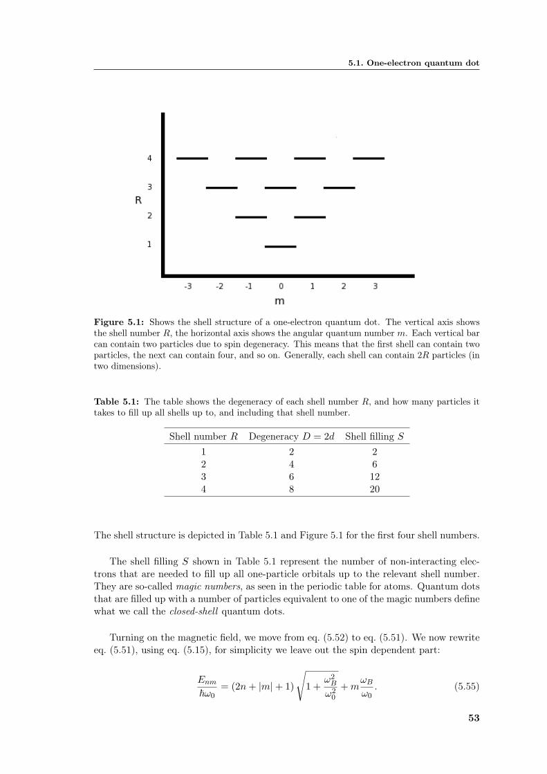
5.1. One-electron quantum dot
Figure 5.1: Shows the shell structure of a one-electron quantum dot. The vertical axis showsthe shell number R, the horizontal axis shows the angular quantum number m. Each vertical barcan contain two particles due to spin degeneracy. This means that the first shell can contain twoparticles, the next can contain four, and so on. Generally, each shell can contain 2R particles (intwo dimensions).
Table 5.1: The table shows the degeneracy of each shell number R, and how many particles ittakes to fill up all shells up to, and including that shell number.
Shell number R Degeneracy D = 2d Shell filling S1 2 22 4 63 6 124 8 20
The shell structure is depicted in Table 5.1 and Figure 5.1 for the first four shell numbers.
The shell filling S shown in Table 5.1 represent the number of non-interacting elec-trons that are needed to fill up all one-particle orbitals up to the relevant shell number.They are so-called magic numbers, as seen in the periodic table for atoms. Quantum dotsthat are filled up with a number of particles equivalent to one of the magic numbers definewhat we call the closed-shell quantum dots.
Turning on the magnetic field, we move from eq. (5.52) to eq. (5.51). We now rewriteeq. (5.51), using eq. (5.15), for simplicity we leave out the spin dependent part:
Enm
~ω0= (2n+ |m|+ 1)
√1 +
ω2B
ω20
+mωB
ω0. (5.55)
53

Chapter 5. Theoretical approximations to quantum dots in two dimensions
0 0.5 1 1.5 2 2.5 3 3.5 40
1
2
3
4
5
6
7
8
9
10Fock−Darwin energy spectrum
ωB/ω0
En
m/hω
0
Figure 5.2: Shows the two-dimensional Fock-Darwin energy spectrum for a single-electron quan-tum dot. When ωB is increased from ωB = 0, the degeneracy in eq. (5.39) is split up. This isbecause of the energy dependence on the sign of m in eq. (5.34). Comparing with 5.1, the shellnumber R = 2 has two possibilities for m, namely m = ±1. This is picture in the figure aboveas a splitting in the energy for Enm/~ω0 = 2 when ωB increases from zero. One path is form = 1, the other is for m = −1. If we were to follow one of the energy lines as ωB increasesfrom zero, the “energy path” of the particle would become a zig-zag line. One line will eventuallycross another line, forming a sudden degeneracy. When ωB is increased further, the particle willchoose the path with the lowest energy (assuming the state is available). Another feature that isclearly visible is the forming of Landau bands. As the magnetic field is increased to the high-fieldlimit, energy states converge to certain Landau levels shown as dotted lines in the figure.
This leads to what is called the Fock-Darwin energy spectrum shown in Figure 5.2. Whenthe magnetic field is off, the energy is degenerate, as shown in Table 5.1 and Figure 5.1.As we turn on the magnetic field, the term m~ωB in eq. (5.51) causes a splitting of thedegenerate states. The energy of the states increases or decreases, depending on the signof m. If we increase ωB further, it causes sudden degeneracies to appear with statesof different shell numbers. If the magnetic field is increased more, a particle in such adegenerate state will choose the state with the most favorable energy (if it is available).Incrementing ωB further leads to new degeneracies, and so on. In the high-field limit(ωB → ∞), the energy lines seem to gather in bands. These bands are called Landaubands (ref. [2]). In this limit, eq. (5.51) reads (without spin energy)
limωB→∞
Enm = (2n+ |m|+ 1 +m)~ωB. (5.56)
We split this equation up in two parts, one for m > 0 and one for m ≤ 0. In the first case
54

5.2. Two-electron quantum dot
we havelim
ωB→∞Enm = (2(n+m) + 1)~ωB, (5.57)
in the second case, the energy becomes independent from m
limωB→∞
En = (2n+ 1)~ωB. (5.58)
We define the Landau band quantum number
NL = 0, 1, 2, .. (5.59)
With this, we can write the high field approximation of the energy as
ENL= (2NL + 1)
ωB
ω0, (5.60)
called Landau energies. We have plotted the first three of these energies in Figure 5.2 asdotted lines. When the magnetic field increases, the Landau bands in the figure convergeto these Landau energies.
Since we have not included the spin energy int eq. (5.55), the lines in Figure 5.2 aredegenerate. Including the spin energy would break each of the lines into two, making theenergy spectra even more complicated.
5.2 Two-electron quantum dot
It has been shown (ref. [34]) that there exists particular analytical solutions of the two-dimensional quantum dot in a homogeneous magnetic field. The solutions exists only forsome particular values of the oscillator frequency in eq. (5.15). This is of importance forus because these analytical solutions gives us a good benchmark for our code when we doour numerical simulations. Our code must be able to reproduce these results.
The Hamiltonian for the two-particle system is
H =2∑
i=1
[1
2m∗ (pi − eAi)2 +
12m∗ω2
0εrr2i
]+
e2
4πε0εrr12, (5.61)
where ε0 is the vacuum permittivity, εr is the relative permittivity, r2i = x2i + y2
i , andr12 = |r2 − r1|. We have not included the spin, because it gives the same addition in theenergy as in the previous section. The only difference now is that we have to sum thecontributions from both of the particles. We assume that the magnetic field is given asB0k, where B0 is a constant and k is the unit vector in z-direction. We want to introducecenter-of-mass coordinates. The transformation is given by
r = r2 − r1, (5.62)
and
R =m1r1 +m2r2
m1 +m2
=r1 + r2
2, (5.63)
55

Chapter 5. Theoretical approximations to quantum dots in two dimensions
where R is the center-of-mass term and r is the relative term. We have used that theparticles are identical, and therefore have identical mass. The momenta transforms inalmost the same way as the coordinates
p =p2 − p1
2, (5.64)
P = p1 + p2. (5.65)
Since the magnetic field is constant, Maxwell’s equations implies that the vector field Amust be linear. This means we transform it as
A(r) = A(r2)−A(r1) (5.66)
A(R) =A(r1) + A(r2)
2(5.67)
We need the following relations when we transform the Hamiltonian:
AR = 2A(R), (5.68)
Ar =12A(r), (5.69)
p21 + p2
2 =12(P2 + 4p2
), (5.70)
r21 + r22 =12(4R2 + r2
), (5.71)
r12 = r, (5.72)
p1 ·A(r1) + p2 ·A(r2) =12P ·AR + 2p ·Ar, (5.73)
A(r1)2 + A(r2)2 =12A2
R + 2A2r, (5.74)
ωR = 2ω0, (5.75)
ωr =12ω0. (5.76)
56

5.2. Two-electron quantum dot
We write out the Hamiltonian
H =1
2m∗[p2
1 + p22 − 2e (p1 ·A(r1) + p2 ·A(r2)) + e2
(A(r1)2 + A(r2)2
)]+
12m∗ω2
0εr(r21 + r22
)+
e2
4πε0εrr
=1
2m∗
[12P2 + 2p2 − 2e
(12P ·AR + 2p ·Ar
)+ e2
(12A2
R + 2A2r
)]+
12m∗ω2
0εr12(4R2 + r2
)+
e2
4πε0εrr
=12
1
2m∗[P2 − 2eP ·AR + e2A2
R
]+
12m2ω2
RR2
+ 2
1
2m∗[p2 − 2ep ·Ar + e2A2
r
]+
12m∗ω2
rr2 +
e2
4πε0εrr
=
12
1
2m∗[P2 − eAR
]2 +12m2ω2
RR2
+ 2
1
2m∗ [p− eAr]2 +
12m∗ω2
rr2 +
e2
4πε0εrr
=
12HR + 2Hr, (5.77)
where we in the last step have defined
HR =1
2m∗[P2 − eAR
]2 +12m2ω2
RR2, (5.78)
and
Hr =1
2m∗ [p− eAr]2 +
12m∗ω2
rr2 +
e2
4πε0εrr. (5.79)
This indicates we can write the wave function in a separable from as
Ψ(R, r) = ψR(R)ψr(r), (5.80)
where the separable solutions are eigenfunctions of the respective Hamiltonians:
HRψR(R) = ERψR(R), (5.81)
andHrψr(r) = Erψr(r). (5.82)
The time independent Schrödinger equation for the whole system is
HΨ(R, r) =(
12HR + 2Hr
)ψ(R)ψ(r)
=12HRψ(R)ψ(r) + 2ψ(R)Hrψ(r)
=(
12ER + 2Er
)ψ(R)ψ(r). (5.83)
The total energy is then
E =12ER + 2Er. (5.84)
57

Chapter 5. Theoretical approximations to quantum dots in two dimensions
We make the following definitions
ωr =
√ω2
r +ω2
B
4=ω
2(5.85)
ωR =√ω2
R + 4ω2B
= 2ω, (5.86)
where ωB and ω is defined as in the previous section. We see that eq. (5.81) is just thesame as the one-particle problem, but with different parameters. We are only interestedin the energy, which is given as
ER = ENM = (2N + |M |+ 1) ~ωR + 2M~ωB
= 2 (2N + |M |+ 1) ~ω + 2M~ωB. (5.87)
The ground state is given by N = M = 0, which gives an energy
ER,0 = 2~ω. (5.88)
Solving eq. (5.82) is in general not possible because of the 1r term in the Hamiltonian.
However, for particular values of ωr it is possible to get closed-form expressions. We referto [34] for a derivation of these solutions. The energies are given as
Er = Enm = (n+ |m|)~ωr +12m~ωB
=12(n+ |m|)~ω +
12m~ωB. (5.89)
The possible solutions are found by first choosing a value for n. This in turn gives a valuefor ω. One problem is that solutions found this way is not always ground states. Thesimplest solutions are generated by n = 2. The frequency is then (ref. [34])
ωr =1
2(2|m|+ 1), (5.90)
or
ω =1
2|m|+ 1, (5.91)
and luckily for us, these are all ground states (ref. [34]). We choose the state with |m| = 0,this gives ω = 1. The energy is then
Er,0 = ~. (5.92)
The total ground-state energy for ω = 1 is found by eq. (5.84). We get E0 = 3~.
For the non-interacting case, the two-particle energy can be found by summing up thetwo lowest energy eigenvalues in eq. (5.44). This gives a ground-state energy of E0 = 2~when ω = 1. This means that in the interacting system, the interaction energy is onethird of the total energy of the system.
58

5.3. The N-electron Hamiltonian
5.3 The N-electron Hamiltonian
For an N -electron system, we need to solve the time-independent Schrödinger equationnumerically. As before, we assume a magnetic field B = B0k, and we approximate theconfining potential with the harmonic oscillator potential. The N-electron Hamiltonianthen reads
H =N∑
i=1
(1
2m∗ (pi − eA)2 +12m∗ω2
0(xi2 + yi
2) + eφ− µi ·B)
+e2
4πε0εr
N∑i<j
1rij. (5.93)
This is almost the same as eq. (5.6), but we have added the electron-electron interaction,and we now sum over several particles. Again, we assume that B = B0k, and do thesame definitions as in Section 5.1. For brevity we set, κ ≡ 4πε0εr~
e2 . The Hamiltonian canthen be written as
H =N∑
i=1
(− ~2
2m∗∇2i − ωBL
(i)z +
12m∗ω2(x2
i + y2i )− gωBS
(i)z
)+
~κ
N∑i<j
1rij, (5.94)
where we have set the term eφ = 0 like before, for the same reason. Both Lz and Sz
commute with the Hamiltonian, m and ms are therefore good quantum numbers. Theeffects of these operators are therefore only constant (dependent only upon the relevantquantum number) additions to the energy (ref. [35]), this means we can write eq. (5.94)as
H =N∑
i=1
(− ~2
2m∗∇2i +
12m∗ω2(x2
i + y2i )− ωB
(m(i) + gm(i)
s
))+
~κ
N∑i<j
1rij. (5.95)
The contributions from the angular and spin part of the Hamiltonian are as stated reallyjust constant additions. This means that there is no reason for us to carry them with usthrough all the calculations; we can just add them after the simulation. This means theHamiltonian we need to simulate is just
H =N∑
i=1
(− ~2
2m∗∇2i +
12m∗ω2(xi
2 + yi2))
+~κ
N∑i<j
1rij. (5.96)
Furthermore, in our simulations, we will only look at closed-shell system. This meansthat all states up to a certain shell is filled. Within a shell, there is a symmetry to thespin and angular quantum number
m = 0,±1,±2, ..,±mmax, (5.97)
ms = ±12, (5.98)
where mmax is the maximum value of the angular quantum number in the relevant shell.When we add the angular and spin energy, the sum goes over all these quantum num-bers. The positive and negative terms will then cancel each other out. Therefore, in aclosed-shell system, there will be no spin and angular addition to the energy. The effectof the external magnetic field is then just to tune the oscillator frequency ω0 → ω.
59
Chapter 5. Theoretical approximations to quantum dots in two dimensions
5.4 Scaling the N-electron Hamiltonian
In order to simplify our calculations later on, we want rescale our Hamiltonian to adimensionless form. First of all, we define a new length unit α. We want to make all thelength units in the Hamiltonian dimensionless. We define
x′ ≡ x
α, y′ ≡ y
α, r′ij ≡
rijα, ∇′ ≡ α∇. (5.99)
We can then rewrite the Hamiltonian:
H =N∑
i=1
(− ~2
2m∗∇2i − ωBL
(i)z +
12m∗ω2(x2
i + y2i )− gωBS
(i)z
)+
~κ
N∑i<j
1rij, (5.100)
=N∑
i=1
(− ~
2m∗α2α2∇2
i +12m∗ω2α2x
2i + y2
i
α2
)+
~κα
N∑i<j
α
rij(5.101)
=N∑
i=1
(− ~2
2m∗α2∇′2
i +12m∗ω2α2
(x′2i + y′2i
))+
~κα
N∑i<j
1r′ij. (5.102)
We want to express the Hamiltonian in a dimensionless form. To do this, we multiply thewhole equation with m∗α2
~2 :
m∗α2
~2H =
N∑i=1
(−1
2∇′2
i +12
(m∗ωα2
~
)2 (x′2i + y′2i
))+m∗α
~κ
N∑i<j
1r′ij. (5.103)
For our purpose, we require that
α =~κm∗ . (5.104)
Putting this back into eq. (5.103), we get
κ2
m∗ H =N∑
i=1
(−1
2∇′2
i +12
(~ωκ2
m∗
)2 (x′2i + y′2i
))+
N∑i<j
1r′ij. (5.105)
We define
H ′ =κ2
m∗ H (5.106)
ω′ =~ωκ2
m∗ . (5.107)
This gives us the final form of our dimensionless Hamiltonian
H ′ =N∑
i=1
(−1
2∇′2
i +12ω′2(x′2i + y′2i )
)+
N∑i<j
1r′ij
(5.108)
where ω′ is a dimensionless oscillator frequency. We are later going to vary this when wecalculate the energy, and see how this change affects the energy. By varying this frequencywe are in effect actually varying the exterior magnetic field.
Using the scaled Hamiltonian, energy is given in units of m∗
κ2 = m∗(
e2
4πε0εr~
)2, which
is called Hartrees (symbol: EH or Ha). Lengths are given in units of m∗
~κ = m∗e2
4πε0εr~2 .
60

Chapter 6
Quantum Monte Carlo
As we already have stated a number of times, it is generally impossible to solve the many-body problem analytically. We therefore need numerical methods to get approximatedresults. Many different many-body techniques have been developed over the years, but inthis thesis we are going to use the Monte-Carlo (MC) method. This method (or rather,series of methods) is an example of what we call an ab initio method. Ab initio is derivedfrom the Latin ab (“from”) and initio (“beginning”). In science the term means somethinglike “from first principles”. A calculation is said to be ab initio if it relies on basic andestablished laws of nature without additional assumptions or special models. In quantummechanics this means that we want to solve the many-body Schrödinger equation fromfundamental physical principles alone.
MC methods are based on using (pseudo-)random numbers — hence the name “MonteCarlo”. Any numerical technique in which random numbers play an essential role can becalled a “Monte Carlo” method, after the famous Mediterranean casino town. Three maintypes of MC simulations can be distinguished (ref. [36])
Direct Monte Carlo, in which random numbers are used to model the effect of com-plicated processes, the details of which are not crucial. An example is the modellingof traffic where the behaviour of cars is determined in part by random numbers.
Monte Carlo integration, which is a method for calculating integrals using randomnumbers. This method is efficient when the integration is over high-dimensionalvolumes.
Metropolis Monte Carlo, in which a sequence of distributions of a system is generatedin a so-called Markov chain. This method allows us to study the static propertiesof classical and quantum many-particle systems.
In this thesis, the first one is not important. The two others, however, are central to ourproblem.
By using random numbers, MC methods are considered stochastic, i. e. non-deterministic,unlike other simulation techniques, such as Hartree Fock, Coupled Cluster Theory andConfiguration Interaction (ref. [37]). There are several Quantum MC techniques suchas diffusion Monte Carlo (DMC), Green’s function Monte Carlo (GFMC), path-integralMonte Carlo (PIMC) and variational Monte Carlo (VMC). The last one is our choice
Chapter 6. Quantum Monte Carlo
method.
In this chapter we will discuss the Monte Carlo method at some length. We start outby discussing random number and pseudo-random numbers. We then explain the basicidea behind Monte Carlo integration and importance sampling. We will look at Markovchains and the Metropolis-Hastings algorithm. We then move on to the Variational prin-ciple, before we discuss the quantum-variational-Monte-Carlo (QVMC) method, whichutilize all of the concepts described before. We briefly discuss another algorithm for find-ing the energy minimum, called the Davidon-Fletcher-Powell algorithm (DFP). At theend of the chapter we discuss the blocking method that deals with correlations in ourresult, and a method called time-step extrapolation, which we use to get more correctresults.
It is advisable that the reader reviews Appendix A before reading this chapter. Somebasic concepts like PDFs and sample error are discussed in this appendix, and we willmake use of the results in this chapter.
6.1 Random numbers
All MC methods are based upon the use of random numbers. Random numbers are char-acterised by the fact that their value cannot be predicted. More precisely, if we constructa sequence of random numbers, the probability density for a new number is independentof all the numbers generated so far (ref. [36]). Pure random numbers may occur in exper-iments; for example the radioactive decay of a nucleus is associated with a pure randomnumber since it is not possible to predict when it will decay. One could therefore in prin-ciple build a device that supplies random number based on such radioactive decay, andindeed this has been done. This is, however, a cumbersome method, and one would inmany instances prefer a method that can reproduce the same sequence of random num-bers when it is necessary to check the consistency and accuracy of the produced results.
In our work, we will use random numbers generated by computers. In all computergenerators the new numbers are generated from the previous ones by a mathematical for-mula (ref. [36]); the new values are in other words fully determined by the previous ones.Luckily, though, the numbers generated by computer algorithms have properties whichmake them suitable for simulations. They are therefore called pseudo-random numbers.The most crucial test of a pseudo-random-number generator is that the mean and vari-ance of the number sequence produced match those of the desired PDF1.
We will usually treat computer-generated numbers as though they are truly random,but in reality there will always exist a correlation between the numbers, and they willhave a period before the same set of random numbers is repeated. The algorithms areusually based on a random seed that starts the sequence of numbers. This means thatif you construct a sequence two times with the same initial seed, the same sequence ofnumbers is produces.
1We advice that the reader review the appendix on statistics for a brief introduction to statistics andPDFs
62
6.2. Monte Carlo integration
6.1.1 Generation of uniform random numbers
We will mostly need random numbers of a uniform distribution. The PDF is given by
ρ(x) =
1b−a for a ≤ x ≤ b,0 else.
(6.1)
These generators will return a random number
r ∈ [a, b], (6.2)
with equal probability for every number in the range. In refs. [36, 38] is described someof the standard methods for generating uniform random numbers.
In most cases, we want a random number, r, in the range
r ∈ [0, 1]. (6.3)
In our computations, we will use library functions to get these numbers.
Uniform random numbers are also of importance because the generation of arbitraryPDFs usually begins by transforming from a uniform distribution.
6.1.2 Generation of Gaussian distributed random number
Besides the uniform random numbers, we are also in need of random numbers that followa Gaussian distribution. They have the PDF
ρ(x) =1√
2πσ2e−
(x−ν)2
2σ2 , (6.4)
where ν is the mean of the distribution, and σ2 is the variance (ref. [38]). We will use alibrary function when we generate these numbers. The standard algorithm for creatingGaussian distributed numbers is based on uniform random numbers. It can be found inref. [38].
For more information on the subject of random and pseudo-random numbers, we referto [38, 39].
6.2 Monte Carlo integration
In quantum mechanics (as well as other fields of physics), one often face the problem ofsolving an integral on the form
I =∫ b
adxf(x). (6.5)
There are plenty of numerical methods to solve such integrals. Standard methods usuallyboil down to evaluating the function on a set of (usually, but not always) equally spacedvalues xi and then evaluate the sum
I =b− a
N
N∑i=1
wif(xi), (6.6)
63

Chapter 6. Quantum Monte Carlo
where N is the number of points evaluated, and wi are some weights that do not dependon f , but determine the accuracy of the method. Equation 6.6 is also used in MC inte-gration, with all weights wi = 1, but the points xi chosen randomly.
When we use random numbers to calculate the integral by eq. (6.5), we have toremember that the random numbers are uniformly distributed. We need to make achange of variables in order to adapt to the integration limits a and b. This is quite easilydone by defining
x = a+ (b− a)y, (6.7)
where y is a random number in the range y ∈ [0, 1]. We further have that
dx = (b− a)dy. (6.8)
Substituting this in eq. (6.5), assuming a 6= b, we get
I =1
b− a
∫ 1
0dyf(x(y)). (6.9)
This together with eq. (6.6) yields the following sum for the MC integration (rememberingwe set the weights ωi = 1)
I =1N
N∑i=1
f(x(yi)). (6.10)
If the random points xi are distributed homogeneously on [0, 1], and if N is sufficientlylarge, the sum in eq. (6.6) yields a result close to the exact integral. This result has acorresponding variance which we write as
σ2 ≈⟨f2⟩− 〈f〉2 , (6.11)
where we have defined
〈f〉 1N
N∑i=1
f(x(yi)), and⟨f2⟩
=1N
N∑i=1
f(x(yi))2. (6.12)
The error is given as2
err2 =σ2
N
err =
√σ2
N(6.13)
which means the error scales as (N)−12 . See Appendix A for a derivation of this equation.
Compared to standard numerical integration techniques, this seems unfavourable.Standard quadrature methods yield an error proportional to N−k with k ≥ 1 (ref. [36]).However, MC integration is more efficient in higher dimensions. To see this, considerintegration of a hypercube with sides L and dimension d. Standard quadrature methods
2For the moment we will assume no correlations in the random numbers. We will later discuss amethod call blocking which deals with correlation.
64

6.2. Monte Carlo integration
has equidistant values for the evaluation points xi. The separation value is h. The numberof integration points in the volume will be
N =(L
h
)d
. (6.14)
And the error in the result scales as N− kd (ref. [36]). The error in MC integration, on the
other hand, is independent of the dimensionality. Comparing this to eq. (6.14), we seethat MC integration is more efficient when d > 2k. Monte-Carlo integration is in additionmuch faster for higher dimensions than standard quadrature methods.
6.2.1 Importance sampling
The scheme described above is very “brute-force”-ish, meaning we do not take into ac-count that the contributions to the integral from different regions in the integrationvolume might vary strongly. Standard MC integration samples the function homoge-neously(meaning that they sample with the uniform distribution), so if the significantcontributions to the integral come from a small region within the integration volume,there will be only a few sample points there. This can lead to large statistical errors.One way to improve upon this is by concentrating the sampling in the regions where |f |happens to be large. This is called importance sampling.
Let ρ(x) be a PDF on [a, b] that has more or less the shape of f(x) in the sense that
f(x)ρ(x)
≈ constant. (6.15)
We require that ∫ b
adxρ(x) = 1. (6.16)
We rewrite eq. (6.5)
I =∫ b
adxf(x)
=∫ b
adxρ(x)
[f(x)ρ(x)
]. (6.17)
Random numbers are generated through the uniform distribution, but we want to generaterandom numbers that follow the distribution of ρ(x). We make a change of variables. Letp(y) be the uniform distribution, then we have
p(y)dy = dy = ρ(x)dx, (6.18)
which yields
y(x) =∫ x
aρ(x′)dx′. (6.19)
If y(x) is invertible, we can find x(y) as well. We then rewrite eq. (6.17) as
I =∫ b
adxρ(x)
[f(x)ρ(x)
]=∫ 1
0dyf(x(y))ρ(x(y))
, (6.20)
65

Chapter 6. Quantum Monte Carlo
where the integration limits have been changed to suit the uniform distribution. Withthe integral on the form of eq. (6.20), we can rewrite eq. (6.6)
I =1N
N∑i=1
f(x(yi))ρ(x(yi))
. (6.21)
We definef(x(yi)) =
f(x(yi))ρ(x(yi))
. (6.22)
The error still scales as in eq. (6.13).
The advantage of such a change of variable (in case ρ(x) follows closely f(x)) is thatthe integrand becomes smooth and we can sample over relevant values for the integrand.This allows us to get a better result while using fewer samples than we would have if wedid not use importance sampling.
6.3 Markov chains and the Metropolis-Hastings algorithm
In a MC calculation we first prepare a system in a configuration, calculate an observable,reconfigure the system, calculate the observable again, and so on. This is done severaltimes, and at the end we calculate the mean of the observable. The question is then: Howdo we choose the configuration of the system for each step?
All MC schemes used are based on Markov processes in order to generate new randomstates/configurations (ref. [38]). The reason for choosing a Markov process is: When aMarkov process is run for a long enough time starting with a random state, we willeventually reach the most likely state of the system (ref. [38]). To reach this distribution,the Markov process needs to obey two important criteria; namely that of ergodicity anddetailed balance. The ergodicity criteria has two conditions (ref. [36]):
1. Every configuration which we want to be included in the ensemble should be acces-sible from every other configuration within a finite number of steps. This propertyis called connectedness or irreducibility.
2. There should be no periodicity. Periodicity means that after visiting a particularconfiguration, it should not be possible to return to the same configuration exceptafter t = nk steps, where n is some positive integer and k is a fixed positive integer.
We will come to the criteria of detailed balance later.
The theory of Markov chains is based on random walks. In a random walk, one de-fines a mathematical entity, called a walker, whose attributes completely define the stateof the system in question. In our case the state of the system refers to the state of amany-electron quantum dot. The walker moves in the state space by a combination ofdeterministic and random displacements from its previous position. This sequence thenforms a chain. This chain is a Markov chain if the state-to-state transition probabilitiesare independent of time and history — that is, they depend only on the current state ofthe system, not on how or when it got there (ref. [39]).
66

6.3. Markov chains and the Metropolis-Hastings algorithm
Assume that the system is described by a PDF ωi(t), where the subscript i denotesthe state of the system, and t denotes the “time”, or Markov step. This is the same assaying that ωi(t) gives us the probability of the configuration i to occur at time t. Wedefine transition probabilities Wij , which brings the system from state j to state i. Wecan then set up the following equation
ωi(t+ ∆t) =∑
j
Wijωj(t), (6.23)
where ∆t is a chosen time step. We require W and ω to be normalized∑i
ωi(t) = 1 (6.24)∑j
Wij = 1, (6.25)
since they are both probabilities. The change in the function ωi(t) from one step to theother is governed by two processes:
1. Going from a configuration i at time t to some other configuration j at time t+ ε.This means there is a decrease in the probability of finding the system in state i.
2. Going from a configuration j at time t to some other configuration i at time t+ ε.This means there is a decrease in the probability of finding the system in state j.
This change can be summed up in the following equation
ωi(t+ ε)− ωi(t) =∑
j
Wijωj(t)−Wjiωi(t) . (6.26)
This equation is a discretized version of what is called the master equation (ref. [36]).
We are trying to find the stationary distribution, also called the steady state of thesystem. In this distribution there will be no noticeable change in the probability for statei during a change in time ε. In other words, we require
ωi(t+ ε) = ωi(t). (6.27)
We can then rewrite eq. (6.26) to∑j
Wijωj(t) =∑
j
Wjiωi(t). (6.28)
We can now omit the t-dependence, since we have assumed ergodicity. It is difficult tofind a general solution to eq. (6.28), but there is a particular solution that is immediatelyrecognizable:
Wijωj = Wjiωi. (6.29)
For all pairs of configurations i and j. This solution is called the detailed balance solution.Picture this in the following way. The different configurations i are buckets, each con-taining an amount ωi of water. We can make connections between each pair of bucketswith pumps. Water is pumped from a bucket i to a bucket j with pumping rate Wijωj .Equation (6.29) then states that the pumping rates between each pair of buckets are
67

Chapter 6. Quantum Monte Carlo
balanced in such a way that the flow from i to j is equal to the flow from j to i. Thevolumes ωi and ωj does not change. This holds for all pairs of buckets. The whole set ofwater volumes in the buckets will remain stationary.
We can rewrite eq. (6.29) on the form
Wij
Wji=ωi
ωj. (6.30)
We (usually) know the probabilities ω, but unfortunately we do not know the analyticform of the transition probabilities Wij . We are, however, free to model it as
Wij = gijAij , (6.31)
where we interpret gij as a trial step probability and Aij as an acceptance probability.There are now two paths to take.
1. We demand that the matrix g is symmetric, this is the same as demanding that theprobability for stepping from i to j is equal to the probability for stepping from jto i. We then have that gij = gji, and we rewrite eq. (6.30) on the form
Aij
Aji=ωi
ωj. (6.32)
We then define the ratioR =
ωi
ωj. (6.33)
This is the procedure in what we call simple Metropolis sampling.
2. Instead of letting each random walker attempt to move to any state with equalprobability as in the simple Metropolis sampling, we can try to guide the walkersin the direction of the steady state. This is called generalized Metropolis sampling.We then need to find an appropriate form of the trial step probabilities gij . Werewrite eq. (6.30) as
Aij
Aji=gjiωi
gijωj. (6.34)
We then define the ratioR =
gjiωi
gijωj. (6.35)
Generalized Metropolis sampling is of greatest use where a transition function/prob-ability gij is known that generates a PDF close to the steady state ω (ref. [39]).
We now introduce the Metropolis-Hastings algorithm. This algorithm was first proposedby Metropolis et al. (ref. ( [40])) in 1953, then for the special case of the Boltzmanndistribution. It was later extended to the more general case in 1970 by W. K. Hastings(ref. [41]). This algorithm can be summarized as follows:
Aij =R if R < 11 if R ≥ 1
, (6.36)
or
Aji =
1R if R ≥ 11 if R < 1
, (6.37)
68

6.4. The variational principle
with R defined as above (either simple or generalized Metropolis sampling). A step fromj to i is accepted with probability Aij , and rejected with probability 1 − Aij . This isusually done by generating a random number r ∈ [0, 1]. If r < Aij , the new state isaccepted, else it is rejected.
It is easy to check that the Metropolis algorithm is consistent with eq. (6.30). Say wewant to use simple Metropolis sampling (the proof is equivalent for generalized Metropolissampling). Then we need to check that eq. (6.32) is satisfied with the choice of theacceptance probabilities. We have to check two cases:
1. R < 1:
Aij = R =ωi
ωj
Aji = 1
Aij
Aji=
ωiωj
1=ωi
ωjQED.
2. R ≥ 1
Aij = 1
Aji =1R
=ωj
ωi
Aij
Aji=
1ωj
ωi
=ωi
ωjQED.
The Metropolis-Hastings algorithm satisfies the conditions for both ergodicity anddetailed balance (ref. [38]). The theory of Markov chains then guarantees that we arriveat the steady state distribution by using the Metropolis-Hastings algorithm.
6.4 The variational principle
The time independent Shcrödinger equation reads
HΨn = EnΨn, (6.38)
where H,Ψn and En is the Hamiltonian, energy eigenfunctions and energy eigenvalues ofthe system under consideration, respectively. In this thesis we want calculate the groundstate energy of the system, E0. Unfortunately, it is usually impossible to solve eq. (6.38)analytically. We can, however, make a guess at the ground state wave function. We definea trial wave function ΨT . The energy associated with this wave function is
ET =〈ΨT |H|ΨT 〉〈ΨT |ΨT 〉
, (6.39)
where the denominator stems from the fact that we have not required ΨT to be normalized.The variational principle then states that
E0 ≤〈ΨT |H|ΨT 〉〈ΨT |ΨT 〉
, (6.40)
69

Chapter 6. Quantum Monte Carlo
which means that expectation value of H, in the (presumably incorrect) state ψT is certainto overestimate the ground state energy. We will in the following prove the variationalprinciple.
Since the eigenstates of H form a complete set, we can expand our trial wave functionin this basis
ΨT =∑
n
cnΨn. (6.41)
We then have that
ET =〈ΨT |H|ΨT 〉〈ΨT |ΨT 〉
=
∞∑n,m=0
c∗ncm〈Ψn|H|Ψm〉
∞∑i,j=0
c∗i cj〈Ψi|Ψj〉
=
∞∑n,m=0
c∗ncmEm〈Ψn|Ψm〉
∞∑i,j=0
c∗i cjδij
=
∞∑n,m=0
c∗ncmEmδnm
∞∑i=0
|ci|2=
∞∑n=0
|cn|2En
∞∑i=0
|ci|2. (6.42)
where we have used that the energy eigenfunctions are orthogonal. By definition, theground state energy is the smallest eigenvalue, that is
E0 < En for n > 0, (6.43)
which means that
ET =
∞∑n=0
|cn|2En
∞∑i=0
|ci|2≥
∞∑n=0
|cn|2E0
∞∑i=0
|ci|2= E0. (6.44)
This inequality will only be an equality when ΨT = Ψ0.
The variational principle gets us an upper bound of the ground state energy E0. Themain goal of our thesis is to approximate this energy. The way we do this is by firstmaking a wave function ansatz
ΨT = ΨT (x, αi), (6.45)
where x is the positions of the particles in the system, and αi is a set of variationalparameters which we introduce to the wave function. The number of variational param-eters usually varies; in this thesis we do not introduce more than two. By introducingthese parameters, the energy ET becomes
ET = ET (αi) (6.46)
Our goal is then to find the minimum of this energy by varying the parameters αi.This is the main concept behind the Variational Monte Carlo (VMC) method. Oneshould note that the degree of accuracy of this method depends on our choice of trialwave function. If we choose a function that does not remotely follow the form of the truewave function, the energy approximation will not be good. Therefore it is important touse our understanding of the physics of the system to construct good trial wave functions.
70

6.5. The quantum variational Monte Carlo method (QVMC)
6.5 The quantum variational Monte Carlo method (QVMC)
In the previous sections, we have discussed basic MC methods. We will now proceed tosee how we make use of these methods to get an estimate of the ground state energy of aquantum mechanical many-particle system, using the QVMC method. We start out withseeing how the actual energy calculation is done, then discuss how the sampling is done.We then set up the actual algorithm. At the end we will discuss what is called impor-tance sampling in the QVMC scheme. This is a way to improve upon the basic algorithm.
6.5.1 Calculating the energy and variance of our system
Given a Hamiltonian, H, the energy of a system is given as the expectation value of theHamiltonian
〈E〉 = ˆ〈H〉 =∫
dτΨ∗T (τ , αi)H(τ )ΨT (τ , αi)∫
dτΨ∗T (τ , α)ΨT (τ , α)
, (6.47)
where we define τ ≡ (x1,x2, ..,xN), and dτ ≡ dx1dx2..dxN , with N as the number ofparticles. We want to calculate this integral for a high number of particles. This integralhas a dimensionality of 2N . When N gets large, MC integration is usually the mostefficient way to evaluate this integral. For brevity, we write ΨT (τ , αi) = ΨT . Werewrite eq. (6.47)
〈E〉 =∫
dτΨ∗T HΨT∫
dτΨ∗T ΨT
(6.48)
=∫
dτΨ∗T (ΨT /ΨT )HΨT∫dτΨ∗
T ΨT(6.49)
=∫
dτ|ΨT |2∫dτ |ΨT |2
HΨT
ΨT(6.50)
=∫
dτρ(τ )EL(τ ), (6.51)
where we have defined a probability density function
ρ(τ ) =|ΨT (τ )|2∫dτ |ΨT (τ )|2
, (6.52)
and the local energy operator
EL(τ) =HΨT (τ )ΨT (τ )
. (6.53)
The local energy is constant if ΨT is an exact eigenfunction of the Hamiltonian. Themore closely ΨT approaches the exact eigenfunction, the less strongly will EL vary withτ (ref. [36]). This means that the variance should go to zero as our trial wave functionapproaches the correct ground state. In most cases we will never get a variance of exactlyzero, because our wave-function ansatz never actually takes the exact form of the correctground state. In Section 9.1.1 we will, however, see that the variance indeed is zero if ourwave-function ansatz is equal to the exact ground state.
71

Chapter 6. Quantum Monte Carlo
We want to solve the integral in eq. (6.51) by MC integration. We do this with aMetropolis random-walk as discussed above. The energy approximation becomes
E ≈ 1M
M∑i=1
EL(Xi), (6.54)
where Xi is the set of sample points, and M is the number of samples. There are twoways to sample the state space of the system. We can use simple Metropolis sampling,or we incorporate importance sampling by using generalized Metropolis sampling. Thesamples are then drawn from the PDF in eq. (6.52).
We also want to calculate the variance. We then need to calculate the energy squared.This is given by
E2 =∫
dτρ(τ )E2L(τ ) ≈ 1
M
M∑i=1
E2L(Xi). (6.55)
The variance is then given byσ2 ≈
⟨E2⟩− 〈E〉2 , (6.56)
and the error is then (by eq. (6.13), still assuming no correlations)
err =
√σ2
N. (6.57)
This means that for each cycle in the MC simulation, we need to calculate the localenergy at the given particle positions. In these calculations, we use the dimensionlessHamiltonian in (5.108), restated here as
H =N∑
i=1
(−1
2∇2
i +12ω(x2
i + y2i ))
+N∑
i<j
1rij. (6.58)
The local energy is then given as
EL(x, y) =1
ΨT
N∑i=1
(−1
2∇2
i +12ω(x2
i + y2i ))
+N∑
i<j
1rij
ΨT ,
= − 1ΨT
N∑i=1
12∇2
i ΨT +N∑
i=1
12ω(x2
i + y2i ) +
N∑i<j
1rij, . (6.59)
From this we calculate both 〈E〉 and⟨E2⟩, giving us an estimate of both the energy and
the variance.
In our thesis, we will try to vary the trial wave function to find an energy minimum. Asstated, if we find the exact ground state, the variance should be zero. This means that onein principle could vary the trial wave function to find the minimum of the variance. Sincewe use a wave-function ansatz, we will in general not find a minimum for the varianceand the energy for the same set of parameters. One could, after the MC simulation, use alinear combination of the parameters that minimize the energy, and the parameters thatminimize the variance to construct the wave function. Indeed, this has proven to yieldthe most efficient wave functions (ref. [42]. We will however not do this, but focus onfinding the parameters that minimize the energy.
72

6.5. The quantum variational Monte Carlo method (QVMC)
6.5.2 Simple Metropolis sampling
Our system is described with the PDF in eq. (6.52). The Metropolis-Hastings algorithmis implemented as follows. For each MC cycle we choose new random positions for theparticles that are dependent on the previous positions. We call this a random walk. Foreach particle, it is done by setting
rnew = rold + ∆rη, (6.60)
where rnew is the new position of the particle, rold is the old position, ∆r is a set steplength, and η is a two-dimensional vector of uniformly distributed random numbers.When the new position for a particle is set, we perform a so-called Metropolis test. Thistest is done to determine if we should accept or reject the new position. We define τ ′ asthe set of particle coordinates where one particle has been moved to a new position, andτ is the set of particle positions where that particle is at the old location. We then definethe ratio according to the simple Metropolis method
R ≡ ρ(τ ′)ρ(τ )
=|ΨT (τ ′)|2
|ΨT (τ )|2, (6.61)
and we define an acceptance probability
A =R if R < 1,1 if R ≥ 1. (6.62)
Finally we compare this with a uniform random number χ. If χ is less than A, we acceptthe new position. If χ is larger than A, the new position is rejected, and we move theparticle back to the old position. After this procedure is done for all particles, we calculatethe local energy, and a new MC cycle can begin.
6.5.3 Generalized Metropolis sampling
The algorithm described above is not optimal. We do not discriminate when we choosenew positions. Typical many-particle wave functions are very small in large parts of con-figuration space, and very large in other parts ( [36]). This means that we might haveproblems in finding regions where the wave function is large, and that attempted movesof walkers from regions where the wave function is large will be rejected with high prob-abilities.
There exist more efficient approaches. The simplest form of the diffusion equation canbe written as
∂ρ(τ , t)∂t
= D∇2ρ(τ , t), (6.63)
where D is the diffusion constant. This equation describes how the probability densityρ(τ , t) of a random walker evolves in time (ref. [36]). We want to construct a Markoviandiffusion process that has a predefined distribution as its stationary distribution. Thenstationary distribution we want to simulate is eq. (6.52). We then modify the simplediffusion equation in eq. (6.63) by adding a drift term that guides the distribution towardsmore likely regions. The Fokker-Planck equation
∂ρ(τ , t)∂t
=N∑
i=1
D∇i (∇i − Fi) ρ(τ , t), (6.64)
73

Chapter 6. Quantum Monte Carlo
describes this Markovian process (ref. [36]). To see this, assume we have reached theinvariant distribution ρ(τ ). Since this is an unchanging state, it is time independent. Wemust have that the left-hand side of eq. (6.64) is zero, namely
N∑i=1
∇i (∇i − Fi) ρ(τ ) = 0. (6.65)
This has the trivial but uninteresting (and unnormalizable) solution ρ = 0. The simplestsolution that makes sense is that each term in the sum is zero. This yields
∇i (∇i − Fi) ρ(τ ) = 0 (6.66)
∇2i ρ(τ ) = ∇i(Fiρ(τ )) (6.67)
∇2i ρ(τ ) = (∇iFi)ρ(τ ) + Fi∇iρ(τ ). (6.68)
This equation has the solution (ref. [39])
Fi =1
ρ(τ )∇iρ(τ ). (6.69)
This drift term causes the diffusion to be biased by ΨT . Equation (6.64) will guide ρ(τ , t)towards the invariant solution ρ(τ ) in a biased way, actually incorporating importancesampling.
Our stationary state is given by eq. (6.52). We then get the following drift term3
Fi =1
Ψ2T
∇iΨ2T
=1
Ψ2T
2ΨT∇iΨT
= 21
ΨT∇iΨT (6.70)
This vector field is usually called the quantum force of the system. Think of it like this:The gradient of the wave function tells us which direction the particles are moving. Thequantum force term then steers our sampling in directions that are more relevant to oursystem, rather than just sampling random points that may actually be of very little inter-est. It actually takes us a bit of time to calculate the quantum force for each MC cycle.However, this is more than made up for by the fact that we need much fewer samples toget a good estimate of the energy.
We now have a diffusion equation which gives the desired distribution. The nextproblem is to implement it using MC. In Statistical mechanics, Fokker-Planck trajecto-ries are generated by means of a Langevin equation (ref. [39]). The Langevin equationcorresponding to eq. (6.64) is
∂r(t)∂t
= DF(r(t)) + η, (6.71)
3We use that our trial state is real, and that the normalization integral is just a constant that iscanceled out in the fraction.
74

6.5. The quantum variational Monte Carlo method (QVMC)
where r(t) is the position of one particle and η is a randomly fluctuating force which isdistributed according to a multidimensional Gaussian with a mean of zero and a varianceof 2D. We integrate this equation over a short time interval ∆t, obtaining a discretizedfrom suitable for our MC calculations. The particle is moved from an old position to anew through
rnew = rold +DF(rold)∆t+ χ√
∆t, (6.72)
where χ is a Gaussian random variable with a mean value of zero and a variance of 2D.So moving to a new position requires that we have an algorithm for creating randomnumbers that follow the distribution in eq. (6.4), with σ2 = 2D, and ν = 0.
The Fokker-Planck equation yields a step probability for the Markov chain given bythe Green’s function (in two dimensions with N particles)
G(τ , τ ′;∆t) =1
(4πD∆t)Ne−
14D∆t
(τ ′−τ−D∆tF(τ ))2 . (6.73)
This function is derived in refs. [36, 39]. If the reader is in need of a deeper introduc-tion to diffusion equations and Green’s functions, we refer to the same references. Thediffusion constant will in our calculations be D = 1
2 . This is found from considering theSchrödinger equation with our dimensionless units.
When we previously discussed Markov chains, we split the transition probability upin two like this:
Wij = gijAij , (6.74)
which is the same as saying
W (τ → τ ′) = g(τ → τ ′)A(τ → τ ′), (6.75)
where τ is the old positions and τ ′ is the new positions. We defined g as a trial stepprobability, and A as an acceptance probability. We now want to use the generalizedMetropolis method as described above. We identify the trial step probabilities g with thegreens function G. We then have
W (τ → τ ′) = G(τ , τ ′;∆t)A(τ → τ ′), (6.76)
and we can rewrite eq. (6.30) as
A(τ → τ ′)A(τ ′ → τ )
=G(τ ′, τ ;∆t)ρ(τ ′)G(τ , τ ′;∆t)ρ(τ )
. (6.77)
We then define the ratio
R =G(τ ′, τ ;∆t)ρ(τ ′)G(τ , τ ′;∆t)ρ(τ )
=G(τ ′, τ ;∆t)|ΨT (τ ′)|2
G(τ , τ ′;∆t)|ΨT (τ )|2. (6.78)
The fraction involving the greens functions becomes
G(τ ′, τ ;∆t)G(τ , τ ′;∆t)
=e−
12∆t(τ−τ ′−∆t
2F(τ ′))2
e−1
2∆t(τ ′−τ−∆t2
F(τ ))2
= e−12(F(τ )+F(τ ′))(∆t
4(F(τ )−F(τ ′))+(τ−τ ′)) (6.79)
75

Chapter 6. Quantum Monte Carlo
Table 6.1: A summary of the QVMC strategy.
Put N walkers at random initial positions.REPEAT for all MC cycles
REPEAT for all walkersSelect next walker, and move that walker to a new position (eitherby eq. (6.60) or by eq. (6.72)).Compute the ratio R (according to either eq. (6.61) or by eq. (6.80)).Accept or reject the new position according to eq. (6.81).
UNTIL we have tried moving all walkers.Update expectation values.
UNTIL all MC cycles is done.
We then rewrite eq. (6.78) as
R =|ΨT (τ ′)|2
|ΨT (τ )|2e−
12(F(τ )+F(τ ′))(∆t
4(F(τ )−F(τ ′))+(τ−τ ′)). (6.80)
The acceptance probability is then defined as before
A =R if R < 1,1 if R ≥ 1. (6.81)
This probability is compared with a uniform random number. If the random number isless than A, we accept the step. If not, we reject it.
In Table 6.1 we have summarized the QVMC algorithm. The strategy is equivalentfor both simple Metropolis sampling and for generalized Metropolis sampling, but theequations used are different.
6.6 Energy minimization using DFP
We wish to minimize the energy using our QVMC machinery. To do this, we need to findthe optimal parameters for our trial wave function, that is, the parameters that minimizesthe expectation value of the energy.
The first strategy that comes to mind is to manually vary the parameters and calcu-late the energy for each set of parameters. However, this is rather brute-force-ish; it doesnot utilize any knowledge of the trial wave function, and it may take us several runs ofthe program to actually target the correct parameters.
Another method we will try out, is the Davidon-Fletcher-Powell algorithm (DFP),given in ref. [43]. This method builds on the conjugate gradient method (CGM), and thesteepest descent method (both of these also described in ref. [43]).
The algorithm is based on approximating a function of variational parameters, f(α),by a quadratic form, where α is a vector of variational parameters. We write f as aTaylor series at around some point P (we choose P as the origin of the coordinate system
76

6.6. Energy minimization using DFP
with coordinates α)
f(α) = f(P) +∑
i
∂f
∂αi
∣∣∣∣P
αi +12
∑ij
∂2f
∂αi∂αj
∣∣∣∣P
αiαj + ...
≈ a− b ·α +12α ·A ·α, (6.82)
where we have defined
a ≡ f(P), b ≡ ∇f |P , Aij =∂2f
∂αi∂αj
∣∣∣∣P
. (6.83)
The matrix A is called the Hessian matrix of the function f at P. In this second orderapproximation, the gradient of f is easily calculated as
∇f = A ·α + b. (6.84)
Calculating the Hessian A is generally hard work. The basic idea the DFP procedureis to build up, iteratively, a good approximation to the inverse Hessian, A−1. This meanswe want to construct a sequence of matrices, Hi, such that
limi→∞
= A−1. (6.85)
DFP is a variant of a variable metric method. Such methods are sometimes calledquasi-Newton methods as well. Consider finding a minimum by using Newton’s methodto search for a zero of the gradient of the function. Near the current point αi, we haveto second order (ref. [43])
f(α = f(αi) + (α−αi) · ∇f(αi) +12(α−αi) ·A · (α−αi), (6.86)
so∇f(α) = ∇f(αi) + A · (α−αi). (6.87)
Using Newton’s method, we set ∇f(α) = 0 to find the next iteration point, which yields
α−αi = −A−1 · ∇f(αi). (6.88)
DFP is called a quasi-Newton method because we do not use the actual Hessian matrixof f , but instead use our current approximation for it. This approach is actually often-times better than using the true Hessian, because we can choose H such that it is alwayspositive definite and symmetric. The true Hessian need not always be so, which may leadto moving towards increasing values of f , as explained in ref. [43].
In ref. [43] there is only given a heuristic motivation for the algorithm which takes Hi
to Hi+1. The algorithm given for updating the matrix is
Hi+1 = Hi +(αi+1 −αi)⊗ (αi+1 −αi)
(αi+1 −αi) · (∇f(αi+1)−∇f(αi))
− [Hi · (∇f(αi+1)−∇f(αi))]⊗ [Hi · (∇f(αi+1)−∇f(αi))](∇f(αi+1)−∇f(αi)) ·Hi · (∇f(αi+1)−∇f(αi))
, (6.89)
77

Chapter 6. Quantum Monte Carlo
where ⊗ denotes the “outer” or “direct” product of two vectors, which will be a matrix.The ij component of u⊗ v is uivj . This algorithm is taken from ref. [43].
Minimization of the function f then entails that we must have algorithms that eval-uates the function itself, evaluates the gradient of the function, ∇f(α), with respectsto the variational parameters. We then choose a matrix H, and update it according toeq. (6.89). We then use the same procedure as in Newton’s method, but with H insteadof the exact Hessian A.
6.7 Blocking
In most of the discussion in this chapter we have completely ignored correlations in theMC results. We have approximated the error in the sample mean with
err2 ≈ 1n
Var(x). (6.90)
The derivation if this equation is shown in Appendix A, and it assumes that the measure-ments are uncorrelated. This is in reality a bad approximation. We are using (pseudo-)random-number generators in many parts of our calculations, and as discussed in Section6.1 there will always be correlations between these random numbers. Even though we haveassumed that the random numbers have little correlations, it turns out that we cannotcompletely ignore the fact that correlations are present. Functions evaluated with respectsto correlated variables will also be correlated. This means that each calculated value ofthe local energy will be correlated to other values. In addition, our algorithm is based onMarkov chains to find new trial positions for the random walkers. A Markov chain, asdiscussed in Section 6.3, contains inherent correlations, because every new Markov stepdepends on the previous position. This is not an independent stochastic process, and weneed to account for the correlations.
As discussed in Appendix A, the effect of correlations in a sample is to increase theerror of the sample mean. When we take correlations in the sample in to considerations,the statistical error for a set of stochastic values is given by
err2 ≈ 1n
Cov(x) =τ
nVar(x), (6.91)
with τ as the autocorrelation time, defined as in eq. (A.39). We have that τ ≥ 1, whereτ = 1 means that the sample is uncorrelated. Calculating τ is rather time consuming,and it is therefore not the best approach for dealing with the correlations. We will insteaduse the blocking technique, described in ref. [44].
The procedure is to group the data into several equal-sized blocks, and then treatthe mean of each block as our measurements. This will leave the mean of the sampleuntouched, but the error will change.
Say we have 10000 measurements. We could then start with an initial block size of 10,this means we have 1000 blocks with 10 measurements in each of the blocks. We treat themean of each block as the new measurements. The total mean of the sample will then beunchanged. We calculate the error of the sample mean, assuming the new measurements
78
6.8. Time-step extrapolation
to be uncorrelated, by eq. (6.90). We then increase the block size, and do a new calcula-tion of the error. This process is repeated. And at some point, we will reach a plateau (wewill see this later when we present our results) where the error does not increase any moreas the block size increases. The error at this plateau will then be our true estimate for thesample error, meaning the measurements (means of each blocks) are in effect uncorrelated.
6.8 Time-step extrapolation
In the generalized Metropolis method, we use the equation
rnew = rold +DF(rold)∆t+ χ√
∆t. (6.92)
to generate trajectories for the particles. Unfortunately, this equation is only exact atthe limit ∆t → 0. However, it is not possible to use ∆t = 0 in the calculations, becausethen the particle would not move at all. This introduces a bias into the dynamics for any∆t > 0. The distribution of trajectories, and therefore the measured energy, will deviateincreasingly from the exact as ∆t increases (ref. [39]).
It is possible to extrapolate towards ∆t = 0 by plotting results for non-zero ∆t andfitting a curve to the data plot. In this work we will use a simple linear fitting that alsoaccommodates for the standard error of the data. We use a least-squares method calledSingular-Value decomposition, described in Section 15.4 in ref. [43].
79


Chapter 7
The trial wave function
We want to find the ground state energy of an N -electron quantum dot. The Hamiltonianof the system is defined in eq. (5.108). We restate it here as
H =N∑
i=1
(−1
2∇2
i +12ω2(x2
i + y2i ))
+N∑
i<j
1rij. (7.1)
As stated before, we simply cannot solve this problem analytically. We therefore need todo numerical calculations. Our method of choice is the QVMC method described in theprevious chapter. But before we can start any calculations, we need a trial wave function.To get a good approximation of the energy, our trial wave function cannot be just anyfunction. We need to employ our understanding of the system to make a good guess athow the analytical form of the wave function actually looks like.
The most commonly used correlated wave function in many-fermion physics is theJastrow-Slater wave function (ref. [9]). This is the wave function we will use in our thesis.The initial assumption is that the wave function can be separated into two parts
ΨT = SJ, (7.2)
where S is a Slater determinant part, and J is some correlation function which we willcall the Jastrow factor.
In this chapter we will find an analytical expression for our trial wave function. Westart out with finding a Slater determinant part that we assume is a good physical de-scription of our system. We will find the single-particle orbitals associated with the Slaterdeterminant, and calculate the gradient and Laplacian of these. We then choose a Jastrowfunction, and discuss the cusp conditions this function must satisfy. At the end we willgive the total trial wave function for our system.
7.1 Slater determinants
We discussed Slater determinants in Chapter 3. The result was that a Slater determinantis an exact solution of the non-interacting system, and that the exact solution to theinteracting system is a linear expansion of Slater determinants. However, this expansionis infinite, and therefore we cannot do it in computer experiments. In this chapter, andthe rest of the thesis, we use the notation |A| for determinants. The matrix associated

Chapter 7. The trial wave function
with the determinant is then written as A.
A general Slater determinant is written
|S| = 1√N !
∣∣∣∣∣∣∣φν1 (x1) · · · φν1 (xN )
......
φνN (x1) · · · φνN (xN )
∣∣∣∣∣∣∣ , (7.3)
where the functions φν are single-particle orbitals, and x = (r, s) as before contains boththe spatial and spin degree of freedom. We restate eq. (3.41), which says that any generalmany-body wave function can be written as a linear combination of Slater determinants
Ψ(x1, ..,xN ) =∑
ν1ν2..νM
Cν1ν2..νM Φν1ν2..νM (x1, ..,xN ), (7.4)
where M is the number of single-particle orbitals, which is generally infinite. Unfortu-nately, we cannot solve an infinite dimensional problem, so we have to cut this sum atsome point. This is why we need to include some extra correlation function to our trialwave function. If we could do the infinite expansion, we would not have to.
We now define the determinant part of our trial wave function as a limited sum
|S′| =c∑i
Ci|Si|, (7.5)
where |Si| represents Slater determinants built up of different sets of single-particle or-bitals, Ci is a set of expansion coefficients, and c is some cutoff that we have defined. Todo QVMC, we want to include some variational parameter, α, to each Slater determinant,i. e.
|Si| → |Si(αi)|. (7.6)
Our trial Slater determinant can then be written as
|S′(αi)| =∑
i
Ci|Si(αi)|. (7.7)
Assume thatφσi , 0 ≤ i < N, (7.8)
is the N single-particle orbitals with lowest energy, where N is the number of particlesin the system. We then define the ground state of the non-interacting system S0 as theSlater determinant that is built up of these orbitals. We rewrite eq. (7.7) as
|S′(αi)| = C0|S0(α0)|+c∑
i=1
Ci|Si(αi)|. (7.9)
The Slater determinant S0 is as stated the ground state of the non-interacting system.We then interpret the other Slater determinants as including correlation effects to thesystem. They do this by introducing single-particle state of higher energy, and then in asense allowing the particles to excite to higher energy levels.
82

7.1. Slater determinants
In our calculations, we will actually only use the ground-state Slater determinant,thereby setting
|S′(α)| = |S0(α)|. (7.10)
This is because we consider a closed shell system. We know that there is a high energydifference between the highest energy state in one shell and the lowest energy state inthe next shell. We make the assumption that it is very hard to excite a particle fromthe outer-most filled shell, and therefore Slater determinants that include orbitals witheven higher energy are very unlikely. This is the same as saying that all the expansioncoefficients in eq. (7.9) are approximately zero, except for C0, which is approximately1. Our Slater determinant does therefore not include any correlation effects, making thechoice of the Jastrow function very important.
7.1.1 Splitting up our Slater determinant
When we later do our actual MC simulation, we will move one particle at the time andevaluate the PDF at the new position. The Slater determinant can be quite tough tocompute, but luckily there are some tricks we can do to make our computations faster.
Our Hamiltonian is spin independent. There are therefore two and two single-particleorbitals that are just the same. It is shown in ref. [9] that when we are calculating theexpectation values of operators that do not depend on spin, we get equivalent results ifwe do the substitution
|S| = 1(N/2)!
|D↑||D↓|, (7.11)
with
|D↑| =
∣∣∣∣∣∣∣∣∣φν1↑ (r1) · · · φν1↑
(rN
2
)...
...φν N
2↑ (r1) · · · φν N
2↑
(rN
2
)∣∣∣∣∣∣∣∣∣ (7.12)
|D↓| =
∣∣∣∣∣∣∣∣∣φν1↓
(r(N
2+1)
)· · · φν1↓ (rN )
......
φν N2↓
(r(N
2+1)
)· · · φν N
2↓ (rN )
∣∣∣∣∣∣∣∣∣ . (7.13)
With the above substitution, even local values of any observables are unchanged, whichis very important for us when we calculate the Local energy at specific points in space.To do the above substitution, we have assumed that we have an even number of particles,with an even number of spin ups and spin downs. This will always be so in a closed-shellsystem. The strength of this substitution is that when we move one particle, only oneof the determinants is changed, and we only have to evaluate this determinant, since wehave stored the value of the other one. This reduces greatly the computation time.
However, if we write our wave function as a separated spin-up and spin-down deter-minant, it will no longer be antisymmetric under particle exchange, as it should be. Evenso, the eigenvalues are unchanged since H is spin independent. Because we work withratios of the wave function in this thesis, we neglect the normalization factors from nowon. These will just cancel out in the total result anyway.
83

Chapter 7. The trial wave function
7.1.2 Single-particle orbitals
We now need to define the single-particle orbitals that make up our Slater determinant.The single-particle orbitals should be the solutions to the one-particle problem associatedwith the Hamiltonian in eq. (7.1)
h = −12∇2 +
12ω2(x2 + y2). (7.14)
We found the solutions to this problem in Section 5.1, but then in polar coordinates. Inthe code we have developed, we use Cartesian coordinates. By examining the one-particleproblem above, we see that it is just the ordinary two-dimensional harmonic oscillatorequation. The solutions to this problem can be found in most standard text books onquantum mechanics (see f. ex. refs. [1, 2]). We write them as
φnx,ny(x, y) = AHnx(√ωx)Hny(
√ωy)e−
ω2 (x2+y2), (7.15)
where A is some normalization constant, and Hnx and Hny are so-called Hermite polyno-mials (see refs. [1, 2]). It is easy to confuse the Hermite polynomials with the Hamiltonian.The way to distinguish them is to remember that the Hermite polynomials always havea subscript n, and the Hamiltonian is usually written in operator form with a hat. Thesingle-particle energies are now given as (remember, we use the scaled Hamiltonian, andthe oscillator frequency ω is the same as defined in eq. (5.107))
Enx,ny = (nx + ny + 1)ω. (7.16)
with
nx = 0, 1, 2, .. (7.17)ny = 0, 1, 2, .. (7.18)
This expression for the energy is a bit different than what we found in eq. (5.44), butremember that our Slater determinant represents a closed-shell system. We have there-fore filled up all single-particle orbitals up to a given shell. The energy of the the Slaterdeterminant is given in eq. (3.37), it is simply the sum of all the single-particle energiesin the determinant. Since we deal with a closed-shell system, the spin and projection ofthe orbital momentum are zero. Defining the single-particle energy as eq. (7.15) thereforeyields the same total energy for the Slater determinant.
We want to introduce some variational parameter to the Slater determinant. We dothis by introducing it in the single-particle orbitals. We then write the orbitals, nowomitting the normalization constant1
φnx,ny(x, y;α) = Hnx(√ωαx)Hny(
√ωαy)e−
ωα2 (x2+y2). (7.19)
7.1.3 Derivatives of the single-particle orbitals
In the MC calculations, we need the gradient and Laplacian of the wave function. Wefirst state an important property of the Hermite polynomials
H ′n(x) = 2nHn−1(x), (7.20)
1We can omit this because all orbitals in the same Slater determinant have the same normalizationfactor. It will then vanish when we compute ratios of the determinants.
84

7.1. Slater determinants
we then have
∂Hnx(√ωαx)
∂x=∂Hnx(
√ωαx)
∂(√ωαx)
∂(√ωαx)∂x
(7.21)
=√ωαH ′
nx(√ωαx) (7.22)
= 2nx
√ωαHnx−1(
√ωαx), (7.23)
and the same applies for Hny(√ωαy). We also find
∂
∂xe−
ωα2 (x2+y2) = ωαxe−
ωα2 (x2+y2). (7.24)
For the sake of brevity, we set Hnx(√ωαx) = Hnx , and Hny(
√ωαy) = Hny . The gradient
of the single-particle orbitals is then
∇φnx,ny(x, y;α) =(i∂
∂x+ j
∂
∂y
)HnxHnye
−ωα2 (x2+y2) (7.25)
= i(∂Hnx
∂xHnye
−ωα2 (x2+y2) +HnxHny
∂
∂xe−
ωα2 (x2+y2)
)+ j(Hnx
∂Hny
∂ye−
ωα2 (x2+y2) +HnxHny
∂
∂ye−
ωα2 (x2+y2)
). (7.26)
We use eq. (7.23) and eq. (7.24) in the last equation, which yields
∇φnx,ny(x, y;α) = i(
2nx
√ωα
Hnx−1
Hnx
− xωα
)HnxHnye
−ωα2 (x2+y2)
+ j(
2ny
√ωα
Hny−1
Hny
− yωα
)HnxHnye
−ωα2 (x2+y2) (7.27)
=((
2nx
√ωα
Hnx−1
Hnx
− xωα
)i
+(
2ny
√ωα
Hny−1
Hny
− yωα
)j)φnx,ny(x, y;α). (7.28)
85

Chapter 7. The trial wave function
We also need to calculate the Laplacian. It is
∇2φnx,ny(x, y;α) = ∇ · ∇φnx,ny(x, y;α) (7.29)
=∂
∂x
((2nx
√ωα
Hnx−1
Hnx
− xωα
)φnx,ny(x, y;α)
)+
∂
∂y
((2ny
√ωα
Hny−1
Hny
− yωα
)φnx,ny(x, y;α)
)(7.30)
=(∂
∂x
(2nx
√ωα
Hnx−1
Hnx
− xωα
)+(
2nx
√ωα
Hnx−1
Hnx
− xωα
)2
+∂
∂y
(2ny
√ωα
Hny−1
Hny
− yωα
)+(
2ny
√ωα
Hny−1
Hny
− yωα
)2)φnx,ny(x, y;α) (7.31)
= ωα
(4nx(nx − 1)
Hnx−2
Hnx
+ 4ny(ny − 1)Hny−2
Hny
+ ωα(x2 + y2
)−4nxx
Hnx−1
Hnx
− 4nyyHny−1
Hny
− 2)φnx,ny(x, y;α). (7.32)
7.2 The Jastrow function
In Chapter 3 we discussed some of the basic properties a fermionic wave function musthave. The Jastrow function needs to emulate the same behaviour. The total wave functionmust be antisymmetric, and we have assumed ΨT = |S|J , where |S| is antisymmetric.The Jastrow function must therefore be symmetric. We also want J to only affect the wavefunction when the distance between particles is reasonably small. The most commonlyused wave function is the Pade-Jastrow function (ref. [39])
J =N∏
i<j
eg(rij) (7.33)
g(rij) =
n∑k=1
aijrkij
1 +n∑
k=1
βkrkij
, (7.34)
where rij is the distance between electron i and electron j, aij is a factor that is dependenton the spin configuration of the particles, and βk is a variational parameter. When thedistance rij becomes small, only the lower order terms in the expansion above is relevant,and one usually use only n = 1, that is
g(rij) =aijrij
1 + βrij, (7.35)
86
7.2. The Jastrow function
which is the analytical form we will use throughout the thesis. Our Jastrow function isthen only
J =∏i<j
eaijrij1+βrij . (7.36)
This function follows the criteria we set in the beginning of the section. In addition itsatisfies important cusp conditions that must be followed.
7.2.1 Cusp conditions
We define the total unnormalized trial wave function as
ΨT = |D↑||D↓|J. (7.37)
The Hamiltonian in eq. (7.1) has a singularity when rij → 0. Since, for any exact eigen-state, HΨ is proportional to Ψ, this divergence must be cancelled by an equal and oppositedivergence in the kinetic energy terms. It is important that this is included in our trialwave function, else the local energy will diverge as rij approaches zero. The divergencycannot be cancelled by the kinetic energy of the Slater determinant part (ref. [39]), so thecancellation must come from the Jastrow factor.
We consider two electrons, k and l, in close approach, and rewrite the Hamiltonian interms of their center-of-mass coordinates, that is
rkl = rl − rk and R =mkrk +mlrl
mk +ml=
rk + rl
2(7.38)
rk = R− rkl
2and rl = R +
rkl
2, (7.39)
where we have used that the particles have equal mass. The gradients in the new coordi-nates transforms as (ref. [45])
∇rkl=
12∇l −
12∇k (7.40)
∇R = ∇k +∇l, (7.41)
which gives12∇2
k +12∇2
l = ∇2rkl
+14∇2
R. (7.42)
With this, the Hamiltonian in eq. (7.1) takes the form
H = −(∇2
rkl+
14∇2
R − 1rkl
)−
N∑i6=k,l
12∇2
i +N∑i
12ω2(x2
i + y2i ) +
N∑(i<j) 6=k,l
1rij. (7.43)
The oscillator energies are finite, as is the kinetic energy of the center-of-mass motion.The Coulomb term 1/rkl, however, diverges as k approaches l. We must have that thekinetic energy term −∇2
rklterm cancels the Coulomb divergence. We consider the local
energy with the these two terms in the limit rkl → 0
limrkl→0
1
|D↑||D↓|J
(−∇2
rkl+
1rkl
)|D↑||D↓|J
<∞, (7.44)
87

Chapter 7. The trial wave function
with rkl = |rkl|. We assume that we have a Pade-Jastrow function on the form ofeq. (7.35). Since we now consider only one pair of particles (the function for all otherpairs of particles will then disappear in the fraction in the expression for the local energy),we write the Jastrow as
J = eg(rkl)∏
(i<j) 6=k,l
eg(rij), (7.45)
with the function g as before. The Laplacian in two dimensions is
∇2r =
1r
∂
∂r+
∂2
∂r2. (7.46)
We then have
∇2rkl|D↑||D↓|J =
(∇2
rkl|D↑||D↓|
)J+2
(∇rkl
|D↑||D↓|)
(∇rklJ)+|D↑||D↓|
(∇2J
). (7.47)
The derivatives of the Jastrow is
∇rJ = rkl∂
∂rkl
eg(rkl)∏
(i<j) 6=k,l
eg(rij)
= g′(rkl)J, (7.48)
and
∇2rJ =
(1r
∂
∂rkl+
∂2
∂r2kl
)eg(rkl)∏
(i<j) 6=k,l
eg(rij)
=(g′(rkl)rkl
+ g′′(rkl) + g′(rkl)2)J, (7.49)
where rkl is a unit vector in the rkl direction. We insert eq. (7.47), eq. (7.48) and eq. (7.49)back into eq. (7.44)
limrkl→0
−∇2
rkl|D↑||D↓|
|D↑||D↓|−
2g′rkl ·(∇rkl
|D↑||D↓|)
|D↑||D↓|−(g′
rkl+ g′′ + g′2 − 1
rkl
)<∞.
(7.50)This equation indicates different short-range behavior for anti-parallel spin than for par-allel spin. For electrons with anti-parallel spin in contact, in general |D↑||D↓| 6= 0, but forelectrons with parallel spin in contact, two rows are the same in one of the determinants,and we must have that |D↑||D↓| = 0. We consider the two cases separately.
1. We first consider anti-parallel spin. With anti-parallel spin, all the terms thatinvolve a derivative of the determinants will be finite. We are left with only twodivergent terms in eq. (7.50), these are the two terms proportional with 1/rkl. Wefind that we must have
limrkl→0
g′ + 1rkl
<∞. (7.51)
To have this we demand that∂g
∂rkl
∣∣∣∣rkl=0
− 1 = 0, (7.52)
which gives the cusp condition
∂g
∂rkl
∣∣∣∣rkl=0
= 1 (7.53)
88

7.3. The total trial wave function
2. For parallel spins we expand |D↑||D↓| around rkl = 0. We get
|D↑||D↓| ≈ b · rkl + .., (7.54)
where b is some undetermined vector. The derivatives are(∇rkl
|D↑||D↓|)∣∣∣
rkl→0≈ b (7.55)(
∇2rkl|D↑||D↓|
)∣∣∣rkl→0
≈ 0 (7.56)
We insert this into eq. (7.50)
limrkl→0
−2g′ (rkl · b)rkl (rkl · b)
−(g′
rkl+ g′′ + g′2 − 1
rkl
)<∞. (7.57)
Collecting all the divergent terms, this yields
limrkl→0
3g′ + 1rkl
<∞. (7.58)
We then demand that
3∂g
∂rkl
∣∣∣∣rkl=0
− 1 = 0, (7.59)
which yields∂g
∂rkl
∣∣∣∣rkl=0
=13. (7.60)
We want to use the Pade-Jastrow function. To find what the cusp conditions imposeon the function we need to find the derivative of g:
g′(rkl) =akl
(1 + βrkl)2(7.61)
g′(0) = akl. (7.62)
To satisfy the cusp condition we demand that
akl =
1 when particles k and l have anti-parallel spin,13 when particles k and l have parallel spin. (7.63)
7.3 The total trial wave function
We have decided on a trial wave function that obeys much of the physics one would expectfrom the correct wave function of the system. Our trial wave function has the form
ΨT (α, β) = |D↑(α)||D↓(α)|J(β), (7.64)
where α and β are two variational parameters which we have imposed on the function.The determinantal part of our function is split into a spin-up and spin-down part. Thisactually destroys the antisymmetric properties of the wave function, but as we havediscussed, it still gives us the correct expectation values. We have chosen a Pade-Jastrow
89

Chapter 7. The trial wave function
function as the correlation function, and found the cusp conditions this function has tosatisfy. The total wave function can then be written as
ΨT =
∣∣∣∣∣∣∣∣∣φν1↑ (r1, α) · · · φν1↑
(rN
2, α)
......
φν N2↑ (r1, α) · · · φν N
2↑
(rN
2, α)∣∣∣∣∣∣∣∣∣
×
∣∣∣∣∣∣∣∣∣φν1↓
(rN
2+1, α
)· · · φν1↓ (rN , α)
......
φν N2↓
(rN
2+1, α
)· · · φν N
2↓ (rN , α)
∣∣∣∣∣∣∣∣∣∏i<j
eaijrij1+βrij , (7.65)
where ri represents the coordinates of particle 1 ≤ i ≤ N . The spin dependent factor inthe Jastrow factor is defined as
aij =
1 when particles i and j have anti-parallel spin,13 when particles i and j have parallel spin, (7.66)
in order to satisfy the cusp condition.
90

Part II
Implementation and results


Chapter 8
Implementation of the QVMCmethod
We implemented the QVMC method by writing a code in C++. This language was chosenbecause of its efficiency and its opportunity for object-orientation. The first step was tobuild a brute-force code to handle the two-particle quantum dot. By brute force we meanthat we used simple Metropolis sampling (see Section 6.5.2). The second step was toimplement generalized Metropolis sampling for the two-electron quantum dot, in order todo a more efficient sampling. The next step was to move on to more particles. We thenneeded efficient algorithms to calculate the Slater determinant and Jastrow factor, andtheir respective derivatives. Since we had an analytical form of the trial wave function,we used analytical derivatives instead of numerical. To make the code more general andadaptive, it has been written in an object-oriented manner. The code can then easilybe used to do QVMC calculations on closed-shell atoms as well, simply by changing thesingle-particle orbitals and the confining potential. The last step was to optimize the codein order to make the calculations as fast as possible. The trial wave function used in thecode is the same as before
ΨT (α, β) = |D↑(α)||D↓(α)|J(β). (8.1)
We start this chapter by giving a description of how we optimize the important cal-culations in our program. We then give a description of the classes in the program andtheir function. We will then describe how the QVMC algorithm has been implemented.We only describe the final QVMC program, not the intermediate ones. This means weonly discuss the generalized Metropolis method, described in Section 6.5.3. We will alsogive a short description as to how we implemented the Davidon-Fletcher-Powell (DFP)algorithm, the blocking technique and time-step extrapolation. Finally, to make our pro-gram more efficient, we have parallelized it. This is shortly discussed at the end of thechapter.
8.1 Optimizing the calculations
If we just raw-coded all the algorithms, the calculations would take a lot of time. Wewant our calculations to be as fast as possible. There are several measures we can taketo achieve this.

Chapter 8. Implementation of the QVMC method
Calculating the determinantal part of the wave function scales as N4 , while the Jas-trow part scales as N3 (ref. [38]). Clearly the Slater determinant scales faster when wesimulate systems with a large number of particles. This means that optimization of ourcode is important in order for us to be able to simulate systems with a large number ofelectrons.
An important observation is that by moving only one electron, we actually only changeone column in only one of the two determinants in eq. (8.1). This is why we split up thedeterminant in the previous chapter. The wave function is needed in three cases:
1. Calculating the acceptance probabilities in the Metropolis-Hastings algorithm
A =R if R < 11 if R ≥ 1,
(8.2)
with R as in eq. (6.80). We concentrate on the part of this ratio that involves onlythe wave function. We write this as
R′2 = R2D↑ ·R2
D↓ ·R2J , (8.3)
where we have defined
RD↑ =|D↑
new||D↑
old|(8.4)
RD↓ =|D↓
new||D↓
old|(8.5)
RJ =Jnew
Jold. (8.6)
The critical observation is that by moving only one particle, only one of the deter-minants is changed. This means that one of the ratios RD↑ , or RD↓ is equal to 1.We can therefore write eq. (8.3) as
R′2 = R2D ·R2
J , (8.7)
where RD is
RD =|Dnew||Dold|
, (8.8)
which is the determinantal ratio that is not equal to one. This ratio is also neededwhen updating the inverse-Slater matrix, as discussed in Section 8.2.2.
2. Calculating the quantum force
Fi = 2∇iΨT
ΨT, (8.9)
where the subscript i means differentiation with respects to particle number i. Wewant to split this up in a Slater part and a Jastrow part. The above equation canbe written as
Fi = 2∇i
(|D↑||D↓|J
)|D↑||D↓|J
= 2(∇i|D↑||D↑|
+∇i|D↓||D↓|
+∇iJ
J
). (8.10)
94

8.1. Optimizing the calculations
Since we differentiate with respects to particle i, the gradient of one of the deter-minants will be zero. We then rewrite the above equation to
Fi = 2(∇i|D||D|
+∇iJ
J
), (8.11)
where we have suppressed the spin configuration of the determinant. This meanswe need algorithms to compute the fractions
GD ≡ ∇i|D||D|
(8.12)
GJ ≡∇iJ
J. (8.13)
3. Calculating the Local energy
EL =∑
i
1ΨT
∇2i ΨT − V, (8.14)
with the potential V as the sum of the harmonic oscillator potential and theCoulomb energy associated with the electron-electron repulsion. The potential en-ergy bit is easy to compute, but we need an efficient algorithm to compute theLaplacian
∇2i ΨT
ΨT=∇2
i
(|D↑||D↓|J
)|D↑||D↓|J
=∇2
i |D↑||D↑|
+∇2
i |D↓||D↓|
+∇2
i J
J+ 2
(∇i|D↑|
) (∇i|D↓|
)|D↑||D↓|
+ 2
(∇i|D↑|
)(∇iJ)
|D↑|J+ 2
(∇i|D↓|
)(∇iJ)
|D↓|J. (8.15)
Once again, only one of the determinants contains the particle i. This means thatthe gradient/Laplacian of the other determinant is zero. The above equation thenreduces to
∇2i ΨT
ΨT=∇2
i |D||D|
+∇2
i J
J+ 2
∇i|D||D|
∇iJ
J. (8.16)
This means we need an algorithm to compute the fractions
LD =∇2
i |D||D|
(8.17)
LJ =∇2
i J
J, (8.18)
in addition to the fractions in eq. (8.12) and eq. (8.13).
In the following we will describe the algorithms used to calculate the various fractions.
8.1.1 The RD-ratio
The inverse of a matrix is related to the determinant of the matrix through (see ref. [3])
D−1 =adj(D)|D|
, (8.19)
95

Chapter 8. Implementation of the QVMC method
where adjD is the adjugate of a matrix. The adjugate of a matrix D is the transpose ofthe cofactor matrix of D (see ref. [3]). We can rewrite eq. (8.19) on matrix-element form
D−1ij =
Cji
|D|, (8.20)
where Cji is the (i, j)-cofactor of D (see ref. [3]). For the matrix D to be invertible, wemust have that D−1D = I, with I as the identity matrix. This can be written as
N∑k=1
DikD−1kj = δij , (8.21)
where δij is the delta function. We multiply eq. (8.20) from the left with Dji, and sumover i, yielding
N∑i=1
DjiD−1ij =
N∑i=1
DjiCji
|D|. (8.22)
This results in
I =N∑
i=1
DjiCji
|D|, (8.23)
or
|D| =N∑
i=1
DjiCji. (8.24)
Using eq. (8.24), we express the ratio in eq. (8.8) as
RD =
N∑i
Dnewji Cnew
ji
N∑i
Doldji C
oldji
. (8.25)
When moving only one particle, lets say particle j, only the j-th row of the matrixchanges. This means that the j-th row of the cofactor matrix will remain unchanged (infact, only the j-th column is unchanged). This means we set
Cnewji = Cold
ji . (8.26)
Equation (8.25) then becomes
RD =
N∑i
Dnewji Cold
ji
N∑i
Doldji C
oldji
(8.27)
Using eq. (8.20), we rewrite this as
RD =
N∑i
Dnewji (Dold
ij )−1
N∑i
Doldji (Dold
ij )−1
(8.28)
96

8.1. Optimizing the calculations
Using eq. (8.21), the sum in the denominator is equal to one. We then have
RD =N∑i
Dnewji (Dold
ij )−1 (8.29)
=N∑i
φi(rnewj )(Dold
ij )−1, (8.30)
where we used that the matrix D has the single-particle orbitals φj(ri) as entries (wherej contains the quantum numbers of the state, and ri is the coordinates of particle i). Thesum in eq. (8.30) is then all we need to evaluate when we calculate the Slater ratio. Thismeans we actually need to keep track of the inverse of the Slater matrix. We will see howwe do this later.
We have implemented eq. (8.30) as shown in the code segment below.
double S l a t e r : : ge t_rat io ( double ∗ r , i n t p) R = 0 ;
f o r ( i n t i = 0 ; i < dim ; i++) r_try [ i ] = r [ i ] ;
p a r t i c l e = p ;
// Get the r a t i o o f the determinantf o r ( i n t i = 0 ; i < slater_dim ; i++)
new_slater [ i ] = o r b i t a l [ i ]−>get_wf ( r_try ) ;R += new_slater [ i ] ∗ i n v e r s e_s l a t e r [ i ] [ p a r t i c l e ] ;
re turn R;
As its input, this function gets the new particle position and the number of the particlethat has been moved. The calculation is done with the old inverse Slater matrix (i. e. thematrix before the move was done). We also store the values of the single-particle orbitalsat the new position, these are needed when we update the inverse-Slater matrix.
8.1.2 The RJ-ratio
Using the Jastrow function in eq. (7.33), the ratio RJ in eq. (8.6)becomes
RJ =
∏i<j
egnewij
∏i<j
egoldij
= e∆J (8.31)
where we have defined∆J ≡
∑i<j
(gnewij − gold
ij
). (8.32)
When we have moved only one particle (say particle k), we have that
gnewij = gold
ij i, j 6= k, (8.33)
97

Chapter 8. Implementation of the QVMC method
which reduces eq. (8.32) to
∆J =k−1∑i=1
(gnewik − gold
ik
)+
N∑i=k+1
(gnewik − gold
ik
)(8.34)
To calculate the Jastrow ratio, we then need to calculate eq. (8.34), and input this ineq. (8.31). The following code segment implements this.
double Jastrow_exp : : ge t_rat io ( double ∗ r , i n t p) // F i r s t copy which p a r t i c l e i s moved and i t s new l o c a t i o np a r t i c l e = p ;f o r ( i n t i = 0 ; i < dimension ; i++)
r_try [ i ] = r [ i ] ;
// Ca l cu la te the new d i s t an c e s between p a r t i c l e s ,// and the new Jastrow func t i on va lue sf o r ( i n t i = 0 ; i < number_part ic les ; i++)
i f ( i != p a r t i c l e ) r_ij_new [ i ] = ca lc_r_i j ( r_try , r_now [ i ] ) ;g_ij_new [ i ] = jas_func−>get_value ( r_ij_new [ i ] , i , p a r t i c l e ) ;
// Ca l cu la te the r a t i o between new and old Jastrow// The matrix g_ij_old has e n t r i e s only above the d iagona l// so we only use theseR = 0 ;f o r ( i n t i = 0 ; i < p a r t i c l e ; i++)
R += g_ij_new [ i ] − g_ij_old [ i ] [ p a r t i c l e ] ;f o r ( i n t i = p a r t i c l e + 1 ; i < number_part ic les ; i++)
R += g_ij_new [ i ] − g_ij_old [ p a r t i c l e ] [ i ] ;
R = exp (R) ;
re turn R;
8.1.3 The GD-ratio
The algorithm we use to compute the ratio in eq. (8.12) is taken from refs. [38, 39]:
∇i|D||D|
=N∑
j=1
(∇iφj(ri))D−1ji . (8.35)
Again, we see that it is actually the inverse of the Slater matrix that is used.
Equation (8.35) is implemented in the following code segment:
void S l a t e r : : get_grad ( double ∗ grad_slater , i n t p) f o r ( i n t i = 0 ; i < dim ; i++)
grad_s late r [ i ] = 0 ;
98

8.1. Optimizing the calculations
f o r ( i n t i = 0 ; i < slater_dim ; i++) // get the g rad i ent from the o r b i t a l c l a s s , r e tu rn s a vec to ro r b i t a l [ i ]−>get_grad ( grad , r_now [ p ] ) ;f o r ( i n t j = 0 ; j < dim ; j++)
grad_s late r [ j ] += grad [ j ] ∗ i n v e r s e_s l a t e r [ i ] [ p ] ;
This function has as its input a vector where the gradient is stored (grad_slater), and theparticle number (p). The function orbital[i]->get_grad(grad, r_now[p]) then calculatesthe gradient of single-particle orbital φj(rp) according to eq. (7.28).
8.1.4 The GJ-ratio
We split eq. (8.13) into coordinate form:
1J
∂J
∂xi. (8.36)
Using the Jastrow in eq. (7.33), the expression above becomes
1J
∂J
∂xi=
1∏Nk<l e
g(rkl)
∂∏N
k<l eg(rkl)
∂xi. (8.37)
The differentiation only affects the terms where either k or l is equal to i. The aboveexpression then reduces to
1J
∂J
∂xi=
i−1∑k=1
1eg(rki)
∂eg(rki)
∂xi+
N∑k=i+1
1eg(rik)
∂eg(rik)
∂xi
=i−1∑k=1
∂g(rki)∂xi
+N∑
k=i+1
∂g(rik)∂xi
=i−1∑k=1
∂gki
∂rki
∂rki
∂xi+
N∑k=i+1
∂gik
∂rik
∂rik∂xi
. (8.38)
We first find
∂rik∂xi
=∂
∂xi
√(xk − xi)2 + (yk − yi)2
= − xk − xi√(xk − xi)2 + (yk − yi)2
=xi − xk
rik∂rki
∂xi=xi − xk
rki. (8.39)
Using the Pade-Jastrow function in eq. (7.35), we find
∂gik
∂rik=
∂
∂rik
aikrik1 + βrik
=aik
(1 + βrik)2. (8.40)
99
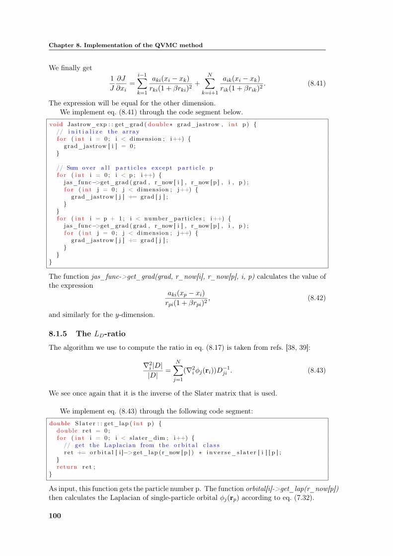
Chapter 8. Implementation of the QVMC method
We finally get1J
∂J
∂xi=
i−1∑k=1
aki(xi − xk)rki(1 + βrki)2
+N∑
k=i+1
aik(xi − xk)rik(1 + βrik)2
. (8.41)
The expression will be equal for the other dimension.We implement eq. (8.41) through the code segment below.
void Jastrow_exp : : get_grad ( double ∗ grad_jastrow , i n t p) // i n i t i a l i z e the arrayf o r ( i n t i = 0 ; i < dimension ; i++)
grad_jastrow [ i ] = 0 ;
// Sum over a l l p a r t i c l e s except p a r t i c l e pf o r ( i n t i = 0 ; i < p ; i++)
jas_func−>get_grad ( grad , r_now [ i ] , r_now [ p ] , i , p ) ;f o r ( i n t j = 0 ; j < dimension ; j++)
grad_jastrow [ j ] += grad [ j ] ;
f o r ( i n t i = p + 1 ; i < number_part ic les ; i++)
jas_func−>get_grad ( grad , r_now [ i ] , r_now [ p ] , i , p ) ;f o r ( i n t j = 0 ; j < dimension ; j++)
grad_jastrow [ j ] += grad [ j ] ;
The function jas_func->get_grad(grad, r_now[i], r_now[p], i, p) calculates the value ofthe expression
aki(xp − xi)rpi(1 + βrpi)2
, (8.42)
and similarly for the y-dimension.
8.1.5 The LD-ratio
The algorithm we use to compute the ratio in eq. (8.17) is taken from refs. [38, 39]:
∇2i |D||D|
=N∑
j=1
(∇2iφj(ri))D−1
ji . (8.43)
We see once again that it is the inverse of the Slater matrix that is used.
We implement eq. (8.43) through the following code segment:
double S l a t e r : : get_lap ( i n t p) double r e t = 0 ;f o r ( i n t i = 0 ; i < slater_dim ; i++)
// get the Laplac ian from the o r b i t a l c l a s sr e t += o r b i t a l [ i ]−>get_lap (r_now [ p ] ) ∗ i n v e r s e_s l a t e r [ i ] [ p ] ;
re turn r e t ;
As input, this function gets the particle number p. The function orbital[i]->get_lap(r_now[p])then calculates the Laplacian of single-particle orbital φj(rp) according to eq. (7.32).
100

8.1. Optimizing the calculations
8.1.6 The LJ-ratio
The derivation of the algorithm used to compute this ratio can be found in ref. [38]. It isa bit tedious, but not really that different from the derivation of the GJ ratio.
As shown in ref. [38], LJ can be written as
LJ = G2J +
i−1∑k=1
(d− 1rki
∂gki
∂rki+∂2gki
∂r2ki
)+
N∑k=i+1
(d− 1rik
∂gik
∂rik+∂2gik
∂r2ik
), (8.44)
where d is the number of dimensions, which in our case is d = 2. We first find, usingeq. (8.40)
∂2gik
∂r2ik=
∂
∂rik
aik
(1 + βrik)2= − 2aikβ
1 + βrik)3. (8.45)
Using eq. (8.40) and eq. (8.45), eq. (8.44) becomes
LJ = G2J +
i−1∑k=1
(1rki
aki
(1 + βrki)2− 2akiβ
1 + βrki)3
)
+N∑
k=i+1
(1rik
aik
(1 + βrik)2− 2aikβ
(1 + βrik)3
)
= G2J +
i−1∑k=1
aki(1− βrki)rki(1 + βrki)3
+N∑
k=i+1
aik(1− βrik)rik(1 + βrik)3
. (8.46)
We implement eq. (8.46) through the following code segment:
double Jastrow_exp : : get_lap ( i n t p) double r e t = 0 ;// We s p l i t the Laplac ian in to two part . The f i r s t one i nvo l v e s// the grad i ent o f the Jastrow func t i onget_grad ( grad_g , p ) ;f o r ( i n t i = 0 ; i < dimension ; i++)
r e t += grad_g [ i ]∗ grad_g [ i ] ;
// The second part i nvo l v e s both the Laplac ian and the grad i ent// o f the Jastrow funct ion , but both o f the se are c o l l e c t e d in to// what we c a l l the Laplac ian in the Pade Jastrow c l a s sf o r ( i n t i = 0 ; i < p ; i++)
r e t += jas_func−>get_lap ( r_ij_old [ i ] [ p ] , i , p ) ;f o r ( i n t i = p + 1 ; i < number_part ic les ; i++)
r e t += jas_func−>get_lap ( r_ij_old [ p ] [ i ] , p , i ) ;re turn r e t ;
The function jas_func->get_lap(r_ij_old[i][p], i, p) calculates the value of the expression
aip(1− βrip)rip(1 + βrip)3
. (8.47)
101

Chapter 8. Implementation of the QVMC method
8.2 Class implementation
The classes of our program are
MC_algo: This is where the Monte Carlo algorithm is implemented. It has a Wave-function object.
Wavefunction: This is an abstract class that contains members that are associated withthe trial wave function.
quantum_dot: This is a derived class from the Wavefunction base class. Specifies aquantum dot wave function. As members it has two Slater objects (one for eachspin configuration), a Jastrow object, and a potential object.
Slater: Class for handling Slater determinants. It has an array of Orbital objects.
Orbital: Class for handling the single-particle orbitals in eq. (7.19), and their derivatives.
Jastrow: Abstract class for handling Jastrow functions.
Jastrow_exp: Derived class from the Jastrow class. Specifies an exponential Jastrowfunction as in eq. (7.33). It has an array of Jastrow_Function objects.
Jastrow_Function: Abstract class that handles the functions in the exponent in anexponential Jastrow factor. It specifies the function g(rij) in eq. (7.33), and thederivatives of this function.
Pade_Jastrow: Derived class from the Jastrow_Function class. Specifies the PadeJastrow function in eq. (7.35).
potential: Abstract class for handling the confining potential in the Hamiltonian.
harm_osc: Derived class from the potential class. Specifies an harmonic oscillator po-tential.
In Figure 8.1 we have included a class diagram of our program.
8.2.1 The initialization of the program
In the main of the program, before we start the MC sampling, we create objects of theclasses.
i n t main ( i n t argc , char ∗argv [ ] ) . . .// I n i t i a l i z a t i o n o f MPI and va r i a b l e s. . .
// Creates a harmonic o s c i l l a t o r p o t e n t i a l ob j e c tp o t e n t i a l ∗ pot = new harm_osc (omega , dimension , number_part ic les ) ;
// Def ine a matrix o f MonteCarlo ob j e c t po i n t e r sMC_algo∗∗∗ paramset = new MC_algo∗∗ [ a lpha_steps ] ;
f o r ( i n t a = 0 ; a < alpha_steps ; a++) paramset [ a ] = new MC_algo∗ [ beta_steps ] ;
102

8.2. Class implementation
−wf : Wavefunction*−random_seed : long−number_cycles : int−number_particles : int−dimension : int−energy2 : double−delta_e : double−time_step : double−greens_function : double−cut_off : int
random_seed : long, number_cycles : int)+get_energy()+get_energy2()+run_algo()
+MC_algo(wf : Wavefunction*, time_step : double
−energy : double
MC_algo
quantum_dot
+quantum_dot(pot : potential*, jas_func : Jastrow_Function*,alpha : double, omega : double,number_particles : int, dimension : int)
+get_potential_energy()+get_kinetic_energy()+~quantum_dot()
−r_prev : double*−grad_slater : double*
−pot : potential*
−slater_dim : int−slater_down : Slater*−particle_tried : int
+try_move(r_try : double*, p : int)
+update()+get_ratio()
+get_slater_grad(slater_grad : double*, particle : int)+local_energy()+get_potential_energy()
−r_now : double**
−grad_jastrow : double*
−dimension : int
−jastrow : Jastrow*
+Wavefunction()+initial_set(r : double**)+calc_ratio(r_try : double*)
+reject_move()
+get_kinetic_energy()
+get_number_particles()+get_dimension()
−R : double
−r_new : double*
−number_particles : int
−slater_up : Slater*
+get_q_force(q_force : double**)
Wavefunction
−r_now : double**−r_ij_old : double**−r_ij_new : double*−jas_func_old : double**−grad : double*−grad_jas : double*−number_particles : int−R : double−dimension : int−particle : int−r_try : double*
+calc_r_ij(r_i : double*, r_j : double*)+Jastrow()+initial_setup(r : double**)+get_ratio(r : double*, p : int)+update()+reject_move()+get_grad()+get_lap()+~Jastrow()
−jas_func_new : double*
Jastrow
−jas_func : Jastrow_Function*
+~Jastrow_exp()+get_lap(p : int)+get_grad(grad_jastrow : double*, p : int)+reject_move()+get_ratio(r : double*, p : int)+initial_setup(r : double**)+Jastrow_exp(jas_func : Jastrow_Function,
number_particles : int, dimension:int)
+update()
Jastrow_exp
−omega : double
+harm_osc(omega : double, dimension : int,number_particles : int)
+get_pot_energy(r : double**)
harm_osc
potential
−number_particles : int−dimension : int
+potential()+get_pot_energy(r : double**)
+Orbital(omega : double, alpha : double,
−alpha : double−dimension : int−omega : double−n : int*−argument : double−state : int−prod : double
dimension : int, state : int)+get_wf(r : double*)+get_grad(grad : double*, r : double*)+get_lap(r : double*)+calculate_r(r : double*)+setup_quantum_numbers(state : int)+~Orbital()
Orbital
−spin_param : double*
+Pade_Jastrow(dimension : int, p_i : int, p_j : int)+get_value(r_ij : double, p_i : int, p_j : int)+get_grad(grad : double*, r_i : double*, r_j : double*,
p_i : int, p_j : int)+get_lap(r_ij : double, p_i : int, p_j : int)+decide_spin_parameter(p_i : int, p_j :int)
Pade_Jastrow
−slater_dim : int−orbital : Orbital**−inverse_slater : double**−old_inv : double**−R : double−r_now : double**−r_try : double*−grad : double*−particle : int−dim : int
+Slater(slater_dim : int, orbital : Orbital**, dimension : int)+initial_setup(r : double**)+get_ratio(r : double*, p : int)+update()+reject_move()+get_grad()+get_lap()+~Slater()
Slater
−beta : double−dimension : int−number_particles : int
+Jastrow_Function()+get_value(r_ij : double, p_i : int, p_j : int)+get_grad(grad : double*, r_i : double*,
+calc_r_ij(r_i : double*, r_j : double*)+get_lap(r_ij : double, p_i : int, p_j : int)+r_j : double*, p_i : int, p_j : int)
Jastrow_Function
Figure 8.1: Class diagram of our QVMC program
103

Chapter 8. Implementation of the QVMC method
f o r ( i n t b = 0 ; b < beta_steps ; b++) // Create a wavefunct ion ob j e c t f o r the s p e c i f i c alpha and betalong idum = −time (NULL) ;#i f MPI_ON == 1idum −= my_rank ;#end i f// Def ine the c o r r e l a t i o n func t i on we ’ re us ingJastrow_Function∗ jas_func =
new Pade_Jastrow ( dimension , beta_start + b∗beta_plus ,number_part ic les ) ;
Wavefunction∗ wf =new quantum_dot ( pot , jas_func , a lpha_start + a∗alpha_plus ,
omega , number_particles , dimension ) ;paramset [ a ] [ b ] = new MC_algo(wf , time_step , idum ,
number_cycles ) ;
. . .
We start by creating an array of MC_algo objects; one for each set of parameters. Eachof the MC_algo objects is given a Wavefunction object of type quantum_dot, and eachquantum_dot objects has two Slater objects, a Jastrow object and a potential object. Inour case, we use the Pade-Jastrow function defined in eq. (7.33) and eq. (7.35), and theSlater determinants use the single-particle orbitals from eq. (7.19). The potential we useis the harmonic oscillator potential
V (x, y) =12ω2(x2 + y2). (8.48)
Inside the main the MC sampling is done through:
i n t main ( i n t argc , char ∗argv [ ] ) . . .// Run the s imu la t i on i t s e l ff o r ( i n t a = 0 ; a < alpha_steps ; a++)
f o r ( i n t b = 0 ; b < beta_steps ; b++) . . .// run the MC algor i thmparamset [ a ] [ b]−>run_algo ( ) ;
// get the energy r e s u l t s from the runenergy = paramset [ a ] [ b]−>get_energy ( ) ;energy2 = paramset [ a ] [ b]−>get_energy2 ( ) ;
tota l_energy = energy ;tota l_energy2 = energy2 ;
#i f MPI_ON == 1// Co l l e c t r e s u l t s from a l l nodesMPI_Reduce(&energy , &total_energy , 1 ,
MPI_DOUBLE, MPI_SUM, 0 , MPI_COMM_WORLD) ;MPI_Reduce(&energy2 , &total_energy2 , 1 ,
MPI_DOUBLE, MPI_SUM, 0 , MPI_COMM_WORLD) ;
tota l_energy /= numprocs ;tota l_energy2 /= numprocs ;#end i f
104

8.2. Class implementation
. . .// Write out to f i l e and measure the time o f the i t e r a t i o n. . .
. . .// F i n a l i z e. . .
We loop over all the different pairs of parameters, and calculate the energy for each pair inthe function paramset[a][b]->run_algo(). Inside this function we start with the followinginitializations:
void MC_algo : : run_algo ( ) . . .// I n i t i a l i z e a r rays and va r i a b l e s. . .
// i n i t i a l t r i a l p o s i t i o nf o r ( i n t i = 0 ; i < number_part ic les ; i++)
f o r ( i n t j = 0 ; j < dimension ; j++) r_old [ i ] [ j ] = gauss ian_deviate (&idum) ∗ s q r t ( time_step ) ;r_new [ i ] [ j ] = r_old [ i ] [ j ] ;
// Get the wave func t i on at these coo rd ina t e swf−>i n i t i a l _ s e t ( r_old ) ;wf−>get_q_force ( q_force_old ) ;
. . .// Do the MC sampling. . .
// end func t i on
We start with setting the initial positions of the particles. Then the wave function isinitialized and the initial quantum force is calculated.
The initialization of the wave function is done through the function wf->initial_set(r_old):
void Wavefunction : : i n i t i a l _ s e t ( double ∗∗ r ) . . .// Copy po s i t i o n. . .
// i n i t i a l i z e S l a t e r determinantsdouble ∗∗ r_1 = ( double ∗∗) matrix ( slater_dim , dimension ,
s i z e o f ( double ) ) ;double ∗∗ r_2 = ( double ∗∗) matrix ( slater_dim , dimension ,
s i z e o f ( double ) ) ;f o r ( i n t i = 0 ; i < slater_dim ; i++)
f o r ( i n t j = 0 ; j < dimension ; j++) r_1 [ i ] [ j ] = r_now [ i ] [ j ] ;
f o r ( i n t i = slater_dim ; i < number_part ic les ; i++)
f o r ( i n t j = 0 ; j < dimension ; j++) r_2 [ i − s later_dim ] [ j ] = r_now [ i ] [ j ] ;
105

Chapter 8. Implementation of the QVMC method
slater_up−>in i t i a l_ s e t up ( r_1 ) ;slater_down−>in i t i a l_ s e t up ( r_2 ) ;
f ree_matr ix ( ( void ∗∗) r_1 ) ; // f r e e memoryfree_matr ix ( ( void ∗∗) r_2 ) ; // f r e e memory
// i n i t i a l i z e Jastrow f a c t o rjastrow−>in i t i a l_ s e t up (r_now ) ;
On input this function gets the initial positions of the particles. The particles are num-bered from 0 to N − 1. It is important that we keep track of the numbering of theseparticles. We define that particles 0 through N/2−1 have spin up, and the rest have spindown. The |D↑| determinant is then initialized with the first half of the particles, andthe |D↓| determinant is initialized with the other half. The numeration of the particlesis also important for the Jastrow factor, in order to decide the value of the parameter ineq. (7.66).
The Slater objects are initialized through:
void S l a t e r : : i n i t i a l_ s e t up ( double ∗∗ r ) . . .// Copy po s i t i o n s. . .
// F i r s t we c a l c u l a t e the S l a t e r matrixf o r ( i n t i = 0 ; i < slater_dim ; i++)
f o r ( i n t j = 0 ; j < slater_dim ; j++) i nv e r s e_s l a t e r [ i ] [ j ] = o r b i t a l [ j ]−>get_wf (r_now [ i ] ) ;
i f ( s later_dim > 1) // Find the i nv e r s e o f the matrix . Function i nv e r s e can be// found in the l i b r a r y f i l e l i b . cppi nv e r s e ( i nve r s e_s l a t e r , s later_dim ) ;
e l s e // I f the S l a t e r matrix only conta in s one pa r t i c l e , the
// func t i on i nv e r s e w i l l not work . We th e r e f o r e need to// do t h i s check , in order f o r the code to work f o r// two p a r t i c l e s
i n v e r s e_s l a t e r [ 0 ] [ 0 ] = 1 ./ i nv e r s e_s l a t e r [ 0 ] [ 0 ] ;
This function first gets a copy of the initial position, then calculates the Slater matrix1.This is done by evaluating the function orbital[j]->get_wf(r_now[i]), which calculatesthe value of the single-particle orbital φj(ri) through eq. (7.19). As we saw in Section 8.1,most of our calculations require the inverse Slater matrix, not the Slater matrix itself.We calculate the inverse matrix using a library function. The Slater matrix itself is notstored, only the inverse matrix.
1The slater matrix is defined as the matrix D associated with the determinant |D|.
106

8.2. Class implementation
The Jastrow function in eq. (7.33) depends on the inter-electron distances rij . If wewrite this as a matrix, it will be symmetrical, which means we only need to store theentries above the main diagonal. When moving one particle, say k, we need to changeonly the entries along column k and row k. As stated above, we use the Pade-Jastrowfunction in eq. (7.35). The values of this function are stored in a matrix. This matrixwill also be symmetric. The Jastrow object is initialized through:
void Jastrow_exp : : i n i t i a l_ s e t up ( double ∗∗ r ) . . .// Copy po s i t i o n s. . .
// Set up the r_ij_old and g_ij_old matr ices ,// making them upper t r i a n gu l a r .// The value o f r_ij_old [ i ] [ j ] i s the d i s t ance// between p a r t i c l e i and p a r t i c l e j .f o r ( i n t i = 0 ; i < number_part ic les ; i++)
f o r ( i n t j = i + 1 ; j < number_part ic les ; j++) r_ij_old [ i ] [ j ] = ca lc_r_i j (r_now [ i ] , r_now [ j ] ) ;g_ij_old [ i ] [ j ] = jas_func−>get_value ( r_ij_old [ i ] [ j ] , i , j ) ;
As its input, this function gets a copy of the position of all the particles. Then the inter-mediate distances, rij , are calculated. The function jas_func->get_value(r_ij_old[i][j],i, j) then calculates the value of gij , according to eq.(7.35).
8.2.2 Implementation of the Metropolis-Hastings algorithm
After the initialization shown in the previous section is done, we are ready to start theMC sampling. This is all done in the function MC_algo::run_algo(). We start out by:
void MC_algo : : run_algo ( ) . . .// I n i t i a l i z a t i o n s. . .// loop over monte c a r l o c y c l e sf o r ( i n t c y c l e s = 1 ; c y c l e s <= number_cycles + cut_of f ; c y c l e s++)
// new po s i t i o nf o r ( i n t i = 0 ; i < number_part ic les ; i++)
f o r ( i n t j = 0 ; j < dimension ; j++) r_new [ i ] [ j ] = r_old [ i ] [ j ] +
(D ∗ q_force_old [ i ] [ j ] ∗ time_step ) +( gauss ian_deviate (&idum) ∗ s q r t ( time_step ) ) ;
. . .
// end func t i on
The array q_force_old[i][j] contains the quantum force (eq. (6.69)) for all the particles atthe old positions. The function gaussian_deviate creates a Gaussian distributed randomnumber. The new positions of the particles moved is calculated through eq. (6.72). Afterthis is done, we tell the wavefunction to try out the new position We calculate the newquantum force, the Green’s function and the ratio between new and old wave function.This is all done through:
void MC_algo : : run_algo ( )
107

Chapter 8. Implementation of the QVMC method
. . .// Try out the new po s i t i o nwf−>try_move (r_new [ i ] , i ) ;. . .
// end func t i on\end l s t l i n s t i n g The func t i on \emphwf−>try \_move( r \_new [ i ] , i ) does the f o l l ow i ng :\ begin l s t l i s t i n g void Wavefunction : : try_move ( double ∗ r_try , i n t p)
. . .// Make a backup o f the p a r t i c l e s o ld po s i t i o n. . .
// Ca l cu la te the r a t i o o f determinants and Jastrowca l c_ra t i o ( r_try ) ;// update determinant and Jastrowupdate ( ) ;
It gets the number of the particle that has been moved, p, and the new position of thisparticle on input. The ratio R′ from eq. (8.3) is then calculated, before the Wavefunctionis updated in the function:
void Wavefunction : : update ( ) // Update s l a t e r determinanti f ( p a r t i c l e_ t r i e d < slater_dim )
slater_up−>update ( ) ;e l s e
slater_down−>update ( ) ;
// Update Jastrow f a c t o rjastrow−>update ( ) ;
// Update po s i t i o n with po in t e r sw i t ch ingdouble ∗ r_temp = r_now [ p a r t i c l e_ t r i e d ] ;r_now [ p a r t i c l e_ t r i e d ] = r_new ;r_new = r_temp ;
This function updates the relevant Slater determinant (i. e. the determinant that containsthe particle that has been moved), and then updates the Jastrow factor.
As we have observed, in the Slater objects we keep track of the inverse-Slater matrix,not the actual Slater matrix. When a particle is moved, we update the inverse matrixthrough an algorithm taken from ref. [39]. We first calculate
Sj ≡N∑
k=1
φk(rnewi )(Dold
kj )−1. (8.49)
The new elements in the inverse matrix are then given as
(Dnewlj )−1 =
(Doldlj )−1 − Sj(D
oldli )−1
RDif j 6= i,
(Doldli )−1
RDif j = i.
(8.50)
The algorithm above is implemented in the following code:
108

8.2. Class implementation
void S l a t e r : : update ( ) . . .// Make a backup o f the matrix in case we r e j e c t the move. . .
// Update the i nv e r s e matrix accord ing to the a lgor i thm// F i r s t we update every column but number pf o r ( i n t i = 0 ; i < p ; i ++)
double S = 0 . 0 ;// Ca l cu la te Sf o r ( i n t j = 0 ; j < slater_dim ; j++)
S += new_slater [ j ] ∗ i n v e r s e_s l a t e r [ j ] [ i ] ;f o r ( i n t j = 0 ; j < slater_dim ; j++)
i nv e r s e_s l a t e r [ j ] [ i ] −= (S/R) ∗ i n v e r s e_s l a t e r [ j ] [ p ] ;
f o r ( i n t i = p + 1 ; i < slater_dim ; i ++)
double S = 0 . 0 ;// Ca l cu la te Sf o r ( i n t j = 0 ; j < slater_dim ; j++)
S += new_slater [ j ] ∗ i n v e r s e_s l a t e r [ j ] [ i ] ;f o r ( i n t j = 0 ; j < slater_dim ; j++)
i nv e r s e_s l a t e r [ j ] [ i ] −= (S/R) ∗ i n v e r s e_s l a t e r [ j ] [ p ] ;
// Update column pf o r ( i n t i = 0 ; i < slater_dim ; i++)
i nv e r s e_s l a t e r [ i ] [ p ] /= R;
. . .// Update p o s i t i o n s. . .
The Jastrow is updated through the function:
void Jastrow_exp : : update ( ) double memory_switch ;// F i r s t update r_nowdouble ∗ temp = r_now [ p a r t i c l e ] ;r_now [ p a r t i c l e ] = r_try ;r_try = temp ; // Old po s i t i o n i s now sto r ed in r_try
// Update r_ij_oldtemp = r_ij_old [ p a r t i c l e ] ;r_ij_old [ p a r t i c l e ] = r_ij_new ;r_ij_new = temp ; // Old r_i j i s now sto r ed in r_ij_new// Al l the new va lues are s to r ed as a row in the matrix// we need to change i t so the matrix i s s t i l l upper d iagona lf o r ( i n t i = 0 ; i < p a r t i c l e ; i++)
memory_switch = r_ij_old [ i ] [ p a r t i c l e ] ;r_ij_old [ i ] [ p a r t i c l e ] = r_ij_old [ p a r t i c l e ] [ i ] ;r_ij_new [ i ] = memory_switch ;
109

Chapter 8. Implementation of the QVMC method
// Update g_ij_old in the same waytemp = g_ij_old [ p a r t i c l e ] ;g_ij_old [ p a r t i c l e ] = g_ij_new ;g_ij_new = temp ; // Old po s i t i o n i s now sto r ed in g_ij_newf o r ( i n t i = 0 ; i < p a r t i c l e ; i++)
memory_switch = g_ij_old [ i ] [ p a r t i c l e ] ;g_ij_old [ i ] [ p a r t i c l e ] = g_ij_old [ p a r t i c l e ] [ i ] ;g_ij_new [ i ] = memory_switch ;
When a particle is moved, lets say particle number p, the only values rij and gij that arechanged are the values where either i or j are equal to p. This means that the valuesalong row p, and column p in the matrices for rij and gij are changed.
After the wave function is updated, we do the following:void MC_algo : : run_algo ( )
. . .// Get new quantum f o r c ewf−>get_q_force ( q_force_new ) ;
// Metropol i s−Hast ings a lgogreens_funct ion = 0 ;f o r ( i n t p = 0 ; p < number_part ic les ; p++)
f o r ( i n t j = 0 ; j < dimension ; j++) greens_funct ion += 0.5 ∗
( q_force_old [ p ] [ j ] + q_force_new [ p ] [ j ] ) ∗(D ∗ time_step ∗ 0 .5 ∗( q_force_old [ p ] [ j ] − q_force_new [ p ] [ j ] ) +r_old [ p ] [ j ] − r_new [ p ] [ j ] ) ;
greens_funct ion = exp ( greens_funct ion ) ;R = wf−>get_rat io ( ) ;R = R∗R;double random = ran2(&idum ) ;double t e s t = greens_funct ion ∗R;
// perform the Metropo l i s t e s ti f ( random <= t e s t )
// Accept the movef o r ( i n t j = 0 ; j < dimension ; j++)
// Update po s i t i o nr_old [ i ] [ j ] = r_new [ i ] [ j ] ;
// Update quantum f o r c e by po in t e r sw i t ch ingdouble ∗∗ temp = q_force_old ;q_force_old = q_force_new ;q_force_new = temp ;
e l s e
// Reject move in the wavefunct ionwf−>reject_move ( ) ;f o r ( i n t j = 0 ; j < dimension ; j++)
// Reset p o s i t i o nr_new [ i ] [ j ] = r_old [ i ] [ j ] ;
110

8.2. Class implementation
. . . end func t i on
The quantum force at the new position is calculated, then the Green’s function (or rather,ratio of Green’s functions) is calculated according to eq. (6.79). Then we calculate theration in eq. (6.80). The Metropolis test is done as described in Section 6.5.3. If the newposition is accepted, we update the positions and quantum force. If it is rejected, we setall the objects back to the old values. This is done in the function wf->reject_move().
After all particles have been tried to be moved, we update the expectation values.This is done through:
void MC_algo : : run_algo ( ) . . .
i f ( c y c l e s > cut_of f ) // compute l o c a l energydelta_e = wf−>loca l_energy ( ) ;// update en e r g i e senergy += delta_e ;energy2 += delta_e ∗delta_e ;
// end o f loop over MC t r i a l s// update the energy average and i t s squareenergy /= number_cycles ;energy2 /= number_cycles ;. . .// Free up memory. . .
// end func t i on
The expectation values are calculated as discussed in Section 6.5.1. The local energy iscalculated as the sum of the kinetic energy and the potential energy. The kinetic energyterm is calculated through
N∑i=1
−12∇iΨT
ΨT=
N∑i=1
−12
(∇2
i |D||D|
+∇2
i J
J+ 2
∇i|D||D|
∇iJ
J
), (8.51)
which is implemented in the following code segment:
double quantum_dot : : get_kinet ic_energy ( ) double r e t = 0 ;// Contr ibut ion from the Laplac ian o f the S l a t e r determinant partf o r ( i n t i = 0 ; i < slater_dim ; i++)
r e t −= slater_up−>get_lap ( i ) ;f o r ( i n t i = 0 ; i < slater_dim ; i++)
r e t −= slater_down−>get_lap ( i ) ;
// Contr ibut ion from the Laplac ian o f the Jastrow partf o r ( i n t i = 0 ; i < number_part ic les ; i++)
r e t −= jastrow−>get_lap ( i ) ;
// Contr ibut ion from the coup l ing o f the S l a t e r determinant// and the Jastrow
111

Chapter 8. Implementation of the QVMC method
f o r ( i n t i = 0 ; i < number_part ic les ; i++) get_slater_grad ( grad_slater , i ) ;jastrow−>get_grad ( grad_jastrow , i ) ;f o r ( i n t i = 0 ; i < dimension ; i++)
r e t −= 2∗ grad_s late r [ i ]∗ grad_jastrow [ i ] ;
re turn 0 .5∗ r e t ;
We could have used numerical derivatives, but since we have an analytical form of thewave function, it is much faster to do analytical derivatives.
The potential energy includes both the harmonic oscillator potential and the Coulombenergy from the electron-electron repulsion. This is calculated in the following codesegment:
double quantum_dot : : get_potent ia l_energy ( ) double e_potent ia l = 0 ;
// F i r s t c a l c u l a t e energy from the coulomb i n t e r a c t i o n between// e l e c t r o n sdouble r_i j ;
f o r ( i n t i = 0 ; i < number_part ic les ; i++) f o r ( i n t j = i + 1 ; j < number_part ic les ; j++)
r_i j = 0 ;f o r ( i n t k = 0 ; k < dimension ; k++)
// c a l c u l a t e s squared d i s t anc e between e l e c t r on i and jr_i j += (r_now [ i ] [ k ] − r_now [ j ] [ k ] ) ∗
(r_now [ i ] [ k ] − r_now [ j ] [ k ] ) ;e_potent ia l += 1 ./ sq r t ( r_ i j ) ;
re turn e_potent ia l + pot−>get_pot_energy (r_now ) ;
The function pot->get_pot_energy(r_now) returns the potential energy from the har-monic oscillator potential at the current position. The local energies for each cycle of theMC sampling is summed up. After all cycles have been finished, we divide the expectationvalues by the number of samples.
8.3 Parallel computing
One of the major strengths of the MC algorithm is that it is very easy to parallelize. Thepossibility of running the program in parallel has been implemented in our code.
Parallel computing means that large tasks are split up in many smaller tasks that aresen to different processes. Each individual process performs its task, and finally all theresults are collected.
In our work, we use the MPI library to parallelize the program. The strategy for our
112

8.4. Implementing the DFP algorithm
program is that we decide on how many codes we want to use, and we then let each pro-cess calculate the expectations values of the energy, and energy squared. Each process isgiven different random seeds, so that they have different initial positions for the particles.If each process then do 106 MC cycles, and we have 10 processes doing calculations, weare in effect doing 107 MC cycles. If we have many processes at our disposal, this willgreatly reduce the time it takes to do a desired amount of MC cycles.
In this work we use the Titan computer cluster for large parallel jobs. The Titancomputer cluster is described on its homepage http://hpc.uio.no.
8.4 Implementing the DFP algorithm
We want to implement the DFP algorithm from Section 6.6. We then implement thefunction dfpmin from ref. [43]. This function utilizes the DFP method to find a minimumof a function f . In our case, this function will be the expectation value of the energydiscussed in Section 6.5.1.
As input, the DFP function needs a pointer to the function it minimizes, as well asa pointer to a function containing the gradient of the function it minimizes. In our casewe want to minimize the energy of a trial wave function. To calculate the energy, we usethe QVMC method. We must also calculate the gradient of the expectation value of theenergy. The partial derivative of 〈E〉 with respects to just one variational parameter is
〈E〉i ≡∂ 〈E〉∂αi
=
⟨ΨT,i
ΨTEL +
HΨT
ΨT− 2 〈E〉
ΨT,i
ΨT
⟩
= 2⟨
ΨT,i
ΨT(EL − 〈E〉)
⟩= 2
⟨ΨT,i
ΨTEL
⟩− 2
⟨ΨT,i
ΨT
⟩〈E〉 , (8.52)
where we have defined ΨT,i = ∂ΨT /∂αi. The expectation values in eq. (8.52) cannoteasily be calculated using closed form expression. In general we must evaluate themnumerically. In this work we use a simple estimate for the first derivative
f ′(x) =f(x+ h)− f(x− h)
h, (8.53)
with h = 0.001.
We have implemented this through the following code segment:
i n t main ( i n t argc , char ∗argv [ ] ) . . .// var i ous d e c l a r a t i o n s and i n i t i a l i z a t i o n s. . .// Do the CGMdfpmin (param , number_parameters , g_tol , &i t e r a t i o n s , &energy ,&E_function , &dE_function ) ;. . .// Pr int out r e s u l t s. . .
dfpmin gets the address of the MC object E_function and the gradient dE_function.The DFP algorithm then uses an MC simulation to calculate the energy. Inside the
113

Chapter 8. Implementation of the QVMC method
MC simulation, we compute derivatives numerically in order to calculate the expectationvalues in eq. (8.52) as well, by:
. . .// MC ca l c u l a t i o n s. . .
// compute l o c a l energydelta_e = wf−>loca l_energy ( ) ;
// Pa r t i a l d e r i v a t i v e swf−>get_part ia l_psi_over_psi ( part ia l_psi_over_psi ,
number_parameters ) ;
// compute expec ta t i on va lue sf o r ( i n t i = 0 ; i < number_parameters ; i++)
exp_val_part_psi_over_psi [ i ] += part ia l_ps i_over_ps i [ i ] ;exp_val_e_local_times_part_psi_over_psi [ i ] +=
delta_e ∗ part ia l_ps i_over_ps i [ i ] ;
// update energyenergy += delta_e ;
// end o f loop over MC t r i a l s// update the expec ta t i on va lue senergy /= number_cycles ;
f o r ( i n t i = 0 ; i < number_parameters ; i++) exp_val_part_psi_over_psi [ i ] /= number_cycles ;exp_val_e_local_times_part_psi_over_psi [ i ] /= number_cycles ;
f o r ( i n t i = 0 ; i < number_parameters ; i++) grad i ent [ i ] = 2 ∗ ( exp_val_e_local_times_part_psi_over_psi [ i ]
− energy ∗exp_val_part_psi_over_psi [ i ] ) ;. . .// f r e e memory and return the energy. . .
This means that when E_function is called, it calculates all the relevant expectation val-ues, and then stores the gradient so that it can be collected when dE_function is called.
8.5 Implementation of blocking
The implementation of the blocking technique discussed in Section 6.7 is rather easy. Thefirst thing we do is to find the optimal parameters by using the QVMC method discussedabove. We then do a single QVMC calculation using the optimal parameters, and storethe local value calculated for each MC loop. We write these values to a file. A separateprogram does the actual blocking. The main of that program looks like this:
i n t main ( i n t nargs , char ∗ args [ ] )
i n t n_procs , min_block_size , max_block_size , n_block_samples , i ;
114

8.5. Implementation of blocking
// The program needs four comand l i n e argumentsi f ( nargs > 4)
n_procs = a t o i ( args [ 1 ] ) ; // F i r s t input i s the number o f// p r o c e s s o r s used in the MPI
min_block_size = a t o i ( args [ 2 ] ) ; // Second input i s the minimum// block s i z e
max_block_size = a t o i ( args [ 3 ] ) ; // Third input i s the maximum// block s i z e
n_block_samples = a t o i ( args [ 4 ] ) ; // Fourth input i s the number// o f b lock samples we want
e l s e
. . .// qu i t program and wr i t e out an e r r o r r epor t. . .
. . .// Co l l e c t the MC r e s u l t s from a l l the nodes used in the s imu la t i on// and i n i t i a l i z e out f i l e. . .
i n t block_size , block_step_length ;double r e s [ 2 ] ;double mean , sigma ;
block_step_length = ( max_block_size − min_block_size ) /n_block_samples ;
// We loop over a l l b lock s i z e sf o r ( i = 0 ; i < n_block_samples ; i++)
b lock_s ize = min_block_size + i ∗ block_step_length ;b lock ing ( mc_results , n , b lock_size , r e s ) ;
mean = re s [ 0 ] ;sigma = re s [ 1 ] ;
. . .// Output. . .
. . .// end program. . .
The program start by reading from the command line the number of processes used whendoing the MC simulations, then reads the minimum and maximum block size we wantto use, and finally the number of block samples we want. Then the values from theMC simulation is collected, before the blocking procedure itself is done. The functionblocking(mc_results, n, block_size, res) looks like:// Finds mean value and var iance o f a block o f a g iven s i z evoid b lock ing ( double ∗ vals , i n t n_vals , i n t block_size , double ∗ r e s )
i n t n_blocks = n_vals/ b lock_s ize ;double ∗ block_vals = new double [ n_blocks ] ;i n t i ;
f o r ( i = 0 ; i < n_blocks ; i++)
115

Chapter 8. Implementation of the QVMC method
block_vals [ i ] = mean( va l s + i ∗ block_size , b lock_s ize ) ;
meanvar ( block_vals , n_blocks , r e s ) ;
d e l e t e block_vals ;
As input it gets an array vals with all the MC values, an integer n_vals that tells thenumber of values in vals, the integer block_size, which tells us the desired block size forthis particular calculation and finally the array res, which is where we return the results.The function mean(vals + i * block_size, block_size) calculates the mean of a block, andthe function meanvar(block_vals, n_blocks, res) calculates the mean and variance of allthe blocks.
8.6 Implementation of time-step extrapolation
To extrapolate the energy and error towards ∆t = 0, we do VMC calculations on severaldifferent values of ∆t, and blocking for each of those values. We then implement anumerical recipe from Section 15.4 in ref. [43], which gives us a linear fitting of theresults, and an estimate of the energy and error at ∆t = 0. The code we use for this isan old FORTRAN code supplied by Morten Hjorth-Jensen.
116

Chapter 9
Computational results
In this chapter we present the results from our simulations. We start out by validatingthat the code yields the correct results for the non-interacting system and the two-particlesystem. We then move on to minimizing the trial wave function for closed-shell systemsof various sizes. We will use brute-force variation (varying the parameters manually), andthe Davidon-Fletcher-Powell (DFP) algorithm to find the optimal parameters. The nextstep is to do blocking and time-step extrapolation with the optimal parameters, in orderto obtain correct results for the energy and the error. We discuss also the dependency onthe oscillator frequency ω. Finally, we will present and discuss the results obtained.
We will mainly consider systems with N ∈ 2, 6, 12, 20, where N is the number ofelectrons in the dot. We will consider oscillator frequencies ω ∈ 0.28, 0.5, 1. At the veryend of the chapter, we will present results for the 30- and 42-electron systems, then onlyconsidering ω = 1.
We use atomic units (a.u.) in all calculations. This corresponds to our scaling of theHamiltonian (see Section 5.4). Energies are then given in units of Hartrees (Ha). We onlyconsider closed-shell systems as discussed in Section 5.1. For brevity we usually only saysystem, but it is implied that we mean closed-shell systems.
9.1 Validating the code
Before we do any large computation, it is important to validate that our code can giveus the correct results for systems where we have analytical values for the energy. Westart out by computing the ground-state energy for the non-interacting system. We thencompute the energy for the two-particle system. If we get good results for these twosystems, we are ready to do computations on more complicated systems.
9.1.1 The non-interacting system
From our discussion in Section 3.3.1, we know that the ground state of the non-interactingsystem can be exactly represented by a Slater determinant filled with the single-particleorbitals with lowest energy eigenvalues. The energy of a single-particle orbital is given ineq. (7.16), and the energy of the Slater determinant is given in eq. (3.37). In Table 9.1 wepresent the analytical energy of the non-interacting system for the first few closed-shellsystems. We have used dimensionless units and the oscillator frequency is set to 1.

Chapter 9. Computational results
Table 9.1: The table shows the energy of a quantum dot with non-interacting particles. Theenergy is calculated for ω = 1 and is given in units of Hartrees.
Shell number R Number of particles Energy (Ha)1 2 22 6 103 12 284 20 60
Table 9.2: In this table we present our results from simulations of a closed-shell quantum dotswith no correlation. The table shows the experimental results for the energy, and the variance.We also include how many MC cycles we have used in the simulations. The energy is given inunits of Hartrees.
Number of particles Energy (Ha) Variance #MC cycles2 2.0000000 σ2 = 0.0000000 106
6 10.000000 σ2 = 0.0000000 106
12 28.000000 σ2 = 0.0000000 106
20 60.000000 σ2 = 0.0000000 106
Our trial wave function is defined as in eq. (7.64), but with no Jastrow factor. Thismeans that our trial wave function is on the correct theoretical form. Our single-particleorbitals are given as in eq. (7.19). The correct orbitals are given in eq. (7.15). This meansthat for α = 1, we should obtain something very close to the exact result.
In our calculations we used an oscillator frequency of ω = 1. We have included theresults of the simulations in Table 9.2. Comparing Table 9.2 to Table 9.1 we see thatwe seem to get the exact results and a variance of zero. This is in agreement with ourdiscussion in Section 6.5.1; the more closely our trial wave function resembles the exactwave function, the less strongly will EL (the local energy) vary with the position. Whenα = 1, our trial wave function is actually the exact wave function of the system. Thismeans that the variance should be equal to zero (except for perhaps some small statisticalfluctuations). In Figure 9.1 we have included a plot that shows how the energy varieswith α. The figure shows a clear minimum for α = 1.
We have also run the code for different values of ω, and reproduced the results pre-dicted by eq. (3.37) and eq. (7.16). That our code is able to reproduce the exact resultsfor the non-interacting system is a clear indication that the Slater determinant part ofour program is correctly coded.
9.1.2 The two-particle case
In Section 5.2 we discussed the two-electron quantum dot, and we found the exact ground-state energy for a dot with an oscillator frequency ω = 1. The energy should be E0 = 3EH
with our scaling of the system. This is a good benchmark to test if our Jastrow part iscoded correct.
118

9.1. Validating the code
0.94 0.96 0.98 1 1.02 1.04 1.0610
10.002
10.004
10.006
10.008
10.01
10.012
10.014
10.016
α
Ene
rgy
(Ha)
Variational plot of a six−particle non−interacting system
Figure 9.1: Shows the variational plot of the non-interacting system for 6 particles. We haveused 1 000 000 Monte-Carlo (MC) cycles for each value of α, and varied α from 0.95 to 1.05 insteps of 0.01. The figure shows a clear minimum for α = 1. Energies are in units of Hartrees.
In this case, we do not know the exact form of the wave function, and it is likely thatour trial wave function does not have the exact form.
We first varied α from 0.5 to 1.4 in steps of 0.1, and β from 0.1 to 1 in steps of 0.1.We did 104 Monte-Carlo (MC) cycles for each iteration. We then closed in on the regionwhere the energy was small. When we closed in on the good values of the variationalparameters, we increased the number of MC cycles.
A final run was made with 100 million cycles. We did 100 variations in both αand β, meaning we had a total of 10 000 iterations. The resulting variational plot of theenergy is shown in Figure 9.2. The optimal parameters are found by considering this plot.
As discussed in Section 6.5.1, a good way to find the ground state could also be tosearch for a minimum in the variance. We will not do this in our later discussion, buttake the time in this section to verify that it is correct. In Figure 9.3 we have included avariational plot of the variance for the two-electron quantum dot.
We collect the results of this section in Table 9.3. We see that we get different pa-rameters depending on whether we choose to minimize the variance or the energy. Thedifferences are not very large, though, which leads us to believe that our wave-functionansatz works quite well for this system. The energy we get is quite close to the exactresult from Section 5.2. The error is calculated according to eq. (A.32), which means wehave assumed no correlations.
119

Chapter 9. Computational results
0.94 0.96 0.98 1 1.02 1.04 1.060.35
0.40.45
3
3.001
3.002
3.003
3.004
3.005
3.006
3.007
3.008
3.009
α
Variational plot of the energy
β
Ene
rgy
in H
a
(a)
0.94 0.96 0.98 1 1.02 1.04 1.063
3.001
3.002
3.003
3.004
3.005
3.006
3.007
3.008
3.009 Energy as a function of α
α
Ene
rgy
in H
a
(b)
0.34 0.36 0.38 0.4 0.42 0.44 0.463
3.001
3.002
3.003
3.004
3.005
3.006
3.007
3.008
3.009 Energy as a function of β
β
Ene
rgy
in H
a
(c)
Figure 9.2: In (a) we have plotted the variational results for the energy for a two-electronquantum dot. The simulation was done with 108 MC samples, and 100 variations in both α andβ. From (b) we read the optimal value of α, and from (c) we read the optimal value of β We findthe minimum at α ≈ 0.987 and β ≈ 0.398. The energy is in units of Hartrees.
Table 9.3: In the first row in the table we present the parameters that minimize the energy,while in the second row we present the parameters that minimize the variance. All results are forthe two-electron quantum dot.
α β Energy (Ha) Variance Error0.987 0.398 〈E〉 = 3.00036 σ2 = 0.00185 4.3012E − 060.980 0.420 〈E〉 = 3.00046 σ2 = 0.00156 3.9497E − 06
120

9.1. Validating the code
0.91
1.11.2
0.340.360.380.40.420.440.460
0.002
0.004
0.006
0.008
0.01
0.012
0.014
0.016
0.018
α
Variational plot of the variance
β
σ2
(a)
0.94 0.96 0.98 1 1.02 1.04 1.060
0.002
0.004
0.006
0.008
0.01
0.012
0.014
0.016
0.018Variance as a function of α
α
σ2
(b)
0.34 0.36 0.38 0.4 0.42 0.44 0.460
0.002
0.004
0.006
0.008
0.01
0.012
0.014
0.016
0.018Variance as a function of β
β
σ2
(c)
Figure 9.3: In (a) we have plotted the variational results for the variance for a two-electronquantum dot. The simulation was done with 108 MC samples. We have done 100 variations inboth α and β. From (b) we read the optimal value of α, and from (c) we read the optimal valueof β. We find the minimum at α ≈ 0.98 and β ≈ 0.42.
121

Chapter 9. Computational results
Table 9.4: In this table we present the optimal parameters found for six-, twelve- and twenty-electron quantum dots, together with a first approximation of the energy for the systems. Theresults are calculated with ω = 1.
N α β Energy (Ha)6 0.92 0.565 〈E〉 = 20.1912 0.87 0.68 〈E〉 = 65.7920 0.84 0.76 〈E〉 = 156.06
To get a more correct estimate for the energy and error, we should do blocking andtime-step extrapolation. We do this in Section 9.3.1.
The code seems to be working well for both the non-interacting and the interactingsystem. We are then ready to do simulations of systems with more electrons.
9.2 Variational plots — Finding the optimal parameters
In this section we will present the result from QVMC simulations on quantum dots withsix, twelve and twenty electrons. We show the variational plots, and find the optimalparameters. All the results presented in this section are calculated with the oscillatorfrequency ω = 1. At the end, we will also present results from the DFP minimization oftwo-, six- and twelve-electron quantum dots.
9.2.1 Simulation of a six-electron quantum dot
To get the optimal parameters for the six-electron system, we first did small calculationsto find the areas of α and β where the energy was small. We then did a large QVMCsimulations with parameters
α ∈ 0.890, 0, 895, 0.900, 0.905, 0.910, 0.915, 0.920, 0.925, 0.930, 0.935 ,β ∈ 0.530, 0.538, 0.546, 0.554, 0.562, 0.570, 0.578, 0.586, 0.594, 0.602 ,
and 100 000 000 MC cycles per iteration. The resulting variational plot of the energy isshown in Figure 9.4.
We have tabulated the results in Table 9.4, together with a first approximation of theenergy of the system. We will do blocking and time-step extrapolation for the optimalparameters in Section 9.3.2 .
9.2.2 Simulation of a twelve-electron quantum dot
We repeat the procedure for the twelve-electron system. In this case it was hard to decideon good optimal parameters, because the function is quite flat in both the α and the βparameter around the minimum. We did a final QVMC simulation with the parameters
α ∈ 0.82, 0.83, 0.84, 0.85, 0.86, 0.87, 0.88, 0.89 ,β ∈ 0.620, 0.635, 0.650, 0.665, 0.680, 0.695, 0.710, 0.725 ,
122

9.2. Variational plots — Finding the optimal parameters
0.880.9
0.920.94
0.52 0.54 0.56 0.58 0.6 0.62
20.19
20.195
20.2
20.205
20.21
20.215
α
Variational plot of the energy
β
Ene
rgy
in H
a
(a)
0.89 0.9 0.91 0.92 0.93 0.94 0.9520.19
20.195
20.2
20.205
20.21
20.215Variational plot of the energy
α
Ene
rgy
in H
a
(b)
0.53 0.54 0.55 0.56 0.57 0.58 0.59 0.6 0.6120.19
20.195
20.2
20.205
20.21
20.215
β
Variational plot of the energy
Ene
rgy
in H
a
(c)
Figure 9.4: In (a) we have plotted the variational results for the energy for a six-electronquantum dot. The simulation was with 108 MC samples. We have done 10 variations in both αand β. From (b) we can read of the optimal value of α, and from (c) we read of the optimal valueof β. We find the minimum at α ≈ 0.920 and β ≈ 0.565.
123
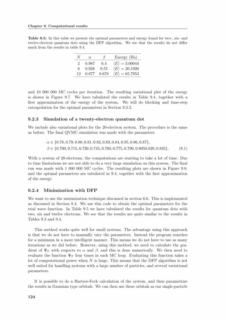
Chapter 9. Computational results
Table 9.5: In this table we present the optimal parameters and energy found for two-, six- andtwelve-electron quantum dots using the DFP algorithm. We see that the results do not differmuch from the results in table 9.4.
N α β Energy (Ha)2 0.987 0.4 〈E〉 = 3.000446 0.928 0.55 〈E〉 = 20.192612 0.877 0.678 〈E〉 = 65.7953
and 10 000 000 MC cycles per iteration. The resulting variational plot of the energyis shown in Figure 9.7. We have tabulated the results in Table 9.4, together with afirst approximation of the energy of the system. We will do blocking and time-stepextrapolation for the optimal parameters in Section 9.3.3.
9.2.3 Simulation of a twenty-electron quantum dot
We include also variational plots for the 20-electron system. The procedure is the sameas before. The final QVMC simulation was made with the parameters
α ∈ 0.78, 0.79, 0.80, 0.81, 0.82, 0.83, 0.84, 0.85, 0.86, 0.87,β ∈ 0.700, 0.715, 0.730, 0.745, 0.760, 0.775, 0.790, 0.8050.820, 0.835. (9.1)
With a system of 20-electrons, the computations are starting to take a lot of time. Dueto time limitations we are not able to do a very large simulation on this system. The finalrun was made with 1 000 000 MC cycles. The resulting plots are shown in Figure 9.8,and the optimal parameters are tabulated in 9.4, together with the first approximationof the energy.
9.2.4 Minimization with DFP
We want to use the minimization technique discussed in section 6.6. This is implementedas discussed in Section 8.4. We use this code to obtain the optimal parameters for thetrial wave function. In Table 9.5 we have tabulated the results for quantum dots withtwo, six and twelve electrons. We see that the results are quite similar to the results inTables 9.3 and 9.4.
This method works quite well for small systems. The advantage using this approachis that we do not have to manually vary the parameters. Instead the program searchesfor a minimum in a more intelligent manner. This means we do not have to use as manyiterations as we did before. However, using this method, we need to calculate the gra-dient of ΨT with respects to α and β, and this is done numerically. We then need toevaluate the function ΨT four times in each MC loop. Evaluating this function takes alot of computational power when N is large. This means that the DFP algorithm is notwell suited for handling systems with a large number of particles, and several variationalparameters.
It is possible to do a Hartree-Fock calculation of the system, and then parametrizethe results in Gaussian type orbitals. We can then use these orbitals as our single-particle
124

9.2. Variational plots — Finding the optimal parameters
0.80.820.840.860.880.9
0.650.7
0.750.8
65.75
65.8
65.85
65.9
65.95
66
α
Variational plot of the energy
β
Ene
rgy
in H
a
(a)
0.8 0.82 0.84 0.86 0.88 0.965.75
65.8
65.85
65.9
65.95
66
α
Variational plot of the energy
Ene
rgy
in H
a
(b)
0.62 0.64 0.66 0.68 0.7 0.72 0.7465.75
65.8
65.85
65.9
65.95
66Variational plot of the energy
β
Ene
rgy
in H
a
(c)
Figure 9.5: In (a) we have plotted the variational results for the energy for a twelve-electronquantum dot. The simulation was with 107 MC samples. We have done 10 variations in both αand β. From (b) we read the optimal value of α, and from (c) we read the optimal value of β.We find the minimum at α ≈ 0.87 and β ≈ 0.68.
125

Chapter 9. Computational results
0.78 0.8 0.82 0.84 0.86 0.880.7
0.80.9
1156.05
156.1
156.15
156.2
156.25
156.3
156.35
156.4
156.45
156.5
β
Variational plot of the energy
α
Ene
rgy
in H
a
(a)
0.78 0.8 0.82 0.84 0.86 0.88156.05
156.1
156.15
156.2
156.25
156.3
156.35
156.4
156.45
156.5
α
Variational plot of the energy
Ene
rgy
in H
a
(b)
0.7 0.75 0.8 0.85156.05
156.1
156.15
156.2
156.25
156.3
156.35
156.4
156.45
156.5Variational plot of the energy
β
Ene
rgy
in H
a
(c)
Figure 9.6: In (a) we have plotted the variational results for the energy for a twenty-electronquantum dot. The simulation was done with 106 MC samples. We have done 10 variations inboth α and β. From (b) we read the optimal value of α, and from (c) we read the optimal valueof β. We find the minimum at α ≈ 0.84 and β ≈ 0.76.
126

9.3. Time-step analysis with blocking
Table 9.6: In this table we give the energy and error calculated with blocking for three valuesof ∆t. In the last row we give the extrapolated result. All values correspond to a quantum dotswith two electrons.
∆t Energy (Ha)0.01 〈E〉 = 3.00026± 3× 10⁻⁵
0.025 〈E〉 = 3.00036± 2× 10⁻⁵
0.05 〈E〉 = 3.00036± 2× 10⁻⁵
Extrapolated: 〈E〉 = 3.00029± 3× 10⁻⁵
orbitals when we construct Slater determinants. These orbitals have already been opti-mized, making the need of the α-parameter superfluous. We then only need to concernourselves with the parameter β. As discussed in Section 8.1, the Slater determinant isthe most costly part of the wave function to calculate. If we only need to minimize thecorrelation function, it would greatly increase the efficiency of the DFP algorithm.
9.3 Time-step analysis with blocking
In this section we will use the optimized parameters found in the previous sections, anddo time-step extrapolation and blocking to get more correct results for the energy andthe error of quantum dots with two, six, twelve and twenty electrons. As described inSections 6.7 and 6.8, blocking is used to get a correct estimate of the error of the samplemean, and time-step extrapolations is done in order to deal with the errors due to thefinite step length in time used in eq. (6.72). All calculations in this section are done withω = 1.
9.3.1 Two electrons
We use the optimal parameters from the energy minimization in Table 9.3. We used threedifferent ∆t values when calculating the energy:
∆t ∈ 0.01, 0.025, 0.05. (9.2)
For each calculation, we use 108 MC cycles. This time we store the local energy calculatedin every single loop of the MC calculation. These values are then loaded in the programdiscussed in Section 8.5. The results are plotted in Figure 9.7. We clearly see the plateaudiscussed in Section 6.7. At this plateau, the blocks are considered to be uncorrelated,and we read of the correct value of the error. In Table 9.6 we give the energy and errorfor the three ∆t-s we have done calculations for. We then do a linear fitting as discussedin Section 8.6. The resulting extrapolated energy and error can also be found in table9.6.
9.3.2 Six electrons
We use the optimal parameters from Table 9.4. We did three calculations of the energywith
∆t ∈ 0.01, 0.025, 0.05,
127

Chapter 9. Computational results
0 2000 4000 6000 8000 100002.25
2.3
2.35
2.4
2.45
2.5
2.55
2.6
2.65x 10
−5
Block size
Err
or
Blocking on 2−electrons with ∆ t = 0.01
0 2000 4000 6000 8000 100002
2.1
2.2
2.3
2.4
2.5
2.6x 10
−4
Block size
Err
or
Blocking on 6−electrons with ∆ t = 0.01
0 2000 4000 6000 8000 100001.54
1.56
1.58
1.6
1.62
1.64
1.66x 10
−5
Block size
Err
or
Blocking on 2−electrons with ∆ t = 0.025
0 2000 4000 6000 8000 100001.44
1.46
1.48
1.5
1.52
1.54
1.56
1.58
1.6
1.62
1.64x 10
−4
Block size
Err
or
Blocking on 6−electrons with ∆ t = 0.025
0 2000 4000 6000 8000 100001.12
1.125
1.13
1.135
1.14
1.145
1.15
1.155
1.16
1.165
1.17x 10
−5
Block size
Err
or
Blocking on 2−electrons with ∆ t = 0.05
0 2000 4000 6000 8000 100001.07
1.08
1.09
1.1
1.11
1.12
1.13
1.14
1.15
1.16x 10
−4
Block size
Err
or
Blocking on 6−electrons with ∆ t = 0.05
Figure 9.7: The plots show the error as a function of block size. To the left in the figure, wesee the blocking plots for the two-electron quantum dot. To the right we see the plots for the six-electron quantum dot. The top two plots are for ∆t = 0.01, the middle plots are for ∆t = 0.025,and the bottom plots are for ∆t = 0.05. The plateau discussed in section 6.7 is clearly visible.At this plateau we find the correct value for the error of the sample mean. If we study the plots,it may seem like the plot is smoother for small values of ∆t. However, by studying the axes, wesee that the resolution is finer for larger ∆t, so the smoothness in the top plots is mostly due toa larger resolution in the y−axis.
128

9.3. Time-step analysis with blocking
Table 9.7: In this table we give the energy and error calculated with blocking for three valuesof ∆t. In the last row we give the extrapolated result. All values correspond to a quantum dotwith six electrons.
∆t Energy (Ha)0.01 〈E〉 = 20.1900± 3× 10⁻⁴
0.025 〈E〉 = 20.1902± 2× 10⁻⁴
0.05 〈E〉 = 20.1904± 1× 10⁻⁴
Extrapolated: 〈E〉 = 20.1899± 2× 10⁻⁴
and 108 MC cycles for each simulation. The resulting blocking plots are presented inFigure 9.7, and we present the energy and error for each ∆t in Table 9.8. In Figure9.8 we have included a plot of the energies and errors from Table 9.8 in order to give avisualisation of how the extrapolation is done.
0 0.01 0.02 0.03 0.04 0.05 0.0620.1896
20.1898
20.19
20.1902
20.1904
20.1906
20.1908
∆ t
Ene
rgy
(Ha)
Plot of the energy and error
Figure 9.8: We have calculated the energy of a six-electron quantum dot using three differentvalues of ∆t. This plot shows the value of the energy for each value of ∆t together with the cor-responding error. The idea is then to make a linear fitting to these points, in order to extrapolatethe value of the energy for ∆t = 0.
9.3.3 Twelve electrons
The same procedure is repeated for the twelve-electron system. We use the optimalparameters from Table 9.6. We calculate the energy for ∆t values:
∆t ∈ 0.01, 0.025, 0.05,
129

Chapter 9. Computational results
Table 9.8: In this table we give the energy and error calculated with blocking for three valuesof ∆t. In the last row we give the extrapolated result. All values correspond to a quantum dotwith twelve electrons.
∆t Energy (Ha)0.01 〈E〉 = 65.7915± 4× 10−04
0.025 〈E〉 = 65.7909± 3× 10−04
0.05 〈E〉 = 65.7901± 2× 10−04
Extrapolated: 〈E〉 = 65.7918± 4× 10⁻⁴
Table 9.9: In this table we give the energy and error calculated with blocking for three valuesof ∆t. In the last row we give the extrapolated result. All values correspond to a quantum dotwith twenty electrons.
∆t Energy (Ha)0.00 〈E〉 = 156.0726± 7× 10−04
0.025 〈E〉 = 156.0695± 4× 10−04
0.05 〈E〉 = 156.0667± 3× 10−04
Extrapolated: 〈E〉 = 156.0732± 6× 10⁻⁴
For each energy calculations, we use 108 MC cycles. The plots are presented in Figure9.9. Once again we see that the error reaches a plateau. We present the calculated energyand error in Table 9.9, together with the extrapolated result.
9.3.4 Twenty electrons
We use the optimal parameters from Table 9.6, and calculate the energy for
∆t ∈ 0.01, 0.025, 0.05,
using 108 MC cycles for each calculation. The resulting blocking plots are presented inFigure 9.9. The plateau value of the error is found, and we present the results in Table9.9.
9.4 Changing the oscillator frequency
We have also done some calculations for oscillator frequencies different from ω = 1.The strategy is as before: We start by finding the optimal variational parameters, thendo blocking and time-step extrapolation to find the energy and error. The results arepresented in Table 9.10. Each calculation of the energy is done with a total of 108 MCcycles.
9.5 Splitting up the energy
We want to see how large the different contributions to the energies are. We can split thetotal energy in three parts:
〈Etot〉 = 〈Ekin〉+ 〈Eosc〉+ 〈Eele〉 , (9.3)
130

9.5. Splitting up the energy
0 2000 4000 6000 8000 100003.5
3.6
3.7
3.8
3.9
4
4.1
4.2
4.3
4.4
4.5x 10
−4
Block size
Err
or
Blocking on 6−electrons with ∆ t = 0.01
0 2000 4000 6000 8000 100005.2
5.4
5.6
5.8
6
6.2
6.4
6.6
6.8x 10
−4
Block size
Err
or
Blocking on 20−electrons with ∆ t = 0.01
0 2000 4000 6000 8000 100002.55
2.6
2.65
2.7
2.75
2.8
2.85
2.9x 10
−4
Block size
Err
or
Blocking on 6−electrons with ∆ t = 0.025
0 2000 4000 6000 8000 100003.75
3.8
3.85
3.9
3.95
4
4.05
4.1
4.15x 10
−4
Block size
Err
orBlocking on 20−electrons with ∆ t = 0.025
0 2000 4000 6000 8000 100001.88
1.9
1.92
1.94
1.96
1.98
2
2.02x 10
−4
Block size
Err
or
Blocking on 6−electrons with ∆ t = 0.05
0 2000 4000 6000 8000 100002.76
2.78
2.8
2.82
2.84
2.86
2.88
2.9
2.92
2.94
2.96x 10
−4
Block size
Err
or
Blocking on 20−electrons with ∆ t = 0.05
Figure 9.9: The plots show the error as a function of block size. To the left in the figure, wesee the blocking plots for the twelve-electron quantum dot. To the right we see the plots forthe twenty-electron quantum dot. The top two plots are for ∆t = 0.01, the middle plots are for∆t = 0.025, and the bottom plots are for ∆t = 0.05. The plateau discussed in section 6.7 isclearly visible. At this plateau we find the correct value for the error of the sample mean. Theapparent differences in smoothness is only due to different resolutions on the y-axis.
131

Chapter 9. Computational results
Table 9.10: In this table we present the optimal parameters and energy found for two-, six-,twelve- and twenty-electron quantum dots calculated for two different values of the oscillatorfrequency.
N ω α β Energy (Ha)2 0.28 0.975 0.25 〈E〉 = 1.02212± 3× 10⁻⁵
0.5 0.98 0.31 〈E〉 = 1.66027± 3× 10⁻⁵
6 0.28 0.88 0.33 〈E〉 = 7.6223± 2× 10⁻⁴
0.5 0.90 0.42 〈E〉 = 11.8104± 2× 10⁻⁴
12 0.28 0.805 0.38 〈E〉 = 25.6989± 4× 10⁻⁴
0.5 0.84 0.48 〈E〉 = 39.2359± 4× 10⁻⁴
20 0.28 0.77 0.42 〈E〉 = 62.0567± 6× 10⁻⁴
0.5 0.81 0.54 〈E〉 = 94.0308± 6× 10⁻⁴
where we have defined:
〈Ekin〉 =
⟨∑i
12∇2
i
⟩, (9.4)
〈Eharm〉 =
⟨∑i
12ω2(x2
i + y2i )
⟩, (9.5)
〈Eele〉 =
⟨∑i<j
1rij
⟩. (9.6)
We then have that 〈Ekin〉 is related to the kinetic energy, 〈Eharm〉 is the energy contribu-tion from the confining potential (in our case a harmonic oscillator potential), and 〈Eele〉is the energy from the Coulomb repulsion between electrons. We want to calculate theexpectation values of each of these energies separately. This is done for the same oscillatorfrequencies used before, and we use the optimal parameters found in Tables 9.3, 9.4 and9.10 for the respective systems. The results are presented in Table 9.11.
9.6 Discussions of the results
We first consider the results in Table 9.11. Varying ω — the oscillator frequency — isequivalent to tuning the confining potential. This means the particles in the dot willbecome more confined when we increase ω, and less confined when we decrease ω. Fromthis reasoning, it seems a bit strange that the role of the energy from the 1/rij term inthe Hamiltonian increases relatively as ω decreases. We shall see why this is so. Ob-viously, the oscillator energy is proportional to ω2, so it is not strange at all that thisenergy decreases relatively with ω. From eq. (7.32), we know that the Laplacian of thesingle-particle orbitals is proportional to ω. This means that the kinetic energy of thedeterminantal part of ΨT will also be proportional to ω, and it follows that this willdecrease with ω. Only the Coulomb energy from the electron-electron repulsion is notdependent on ω (it will, of course, be changed a bit by the fact that the inter-electrondistances are changed, but there is no explicit dependency).
132

9.6. Discussions of the results
Table 9.11: In this table we present the results from calculating the expectation value of eachpart of the total energy separately. All energies are in units of Hartrees. We have used ∆t = 0.05in all calculations. In the parentheses behind the numbers we have included what percentage therelevant energy is of the total energy.
N ω Etot Ekin Eosc Eele
2 0.28 1.0222 0.2531 (24.8%) 0.4235 (41.4%) 0.3456 (33.8%)0.5 1.6602 0.4466 (26.9%) 0.7008 (42.2%) 0.5130 (30.9%)1 3.0004 0.8908 (29.7%) 1.2955 (43.2%) 0.8141 (27.1%)
6 0.28 7.6218 0.9441 (12.4%) 2.8109 (36.9%) 3.8668 (50.7%)0.5 11.8102 1.7213 (14.6%) 4.4772 (37.9%) 5.6117 (47.5%)1 20.1902 3.5831 (17.8%) 7.9234 (39.2%) 8.6837 (43.0%)
12 0.28 25.7003 2.1780 (8.5%) 9.3232 (36.3%) 14.1991 (55.2%)0.5 39.2354 4.0757 (10.4%) 14.5713 (37.1%) 20.5884 (52.5%)1 65.7906 8.8318 (13.4%) 24.7721 (37.7%) 32.1867 (48.9%)
20 0.28 62.055 4.175 (6.7%) 21.804 (35.1%) 36.076 (58.1%)0.5 94.028 7.976 (8.5%) 33.519 (35.6%) 52.533 (55.9%)1 156.068 17.416 (11.2%) 56.995 (36.5%) 81.657 (52.3%)
When ω decreases, interactions get more and more important, and the kinetic energydiminishes. This means that 〈p〉 can be determined very sharply. The uncertainty rela-tion tells us that 〈r〉 (the expectation value of the position) must then increase. This issomething we expect as the particles gets less and less confined when ω decreases.
We can also draw some conclusions from the optimal parameters of the trial wavefunctions of the respective systems. The parameter β is associated with the Jastrow fac-tor in eq. (7.35). When this parameter is small, it means that the Jastrow factor becomeslarge, and it follows that the correlation part of the wave function is more important.Studying Table 9.4, we see that the parameter β increases as N increases. This meansthat the Jastrow part of our trial wave function becomes less important for systems witha higher number of particles, even though the energy from the electron-electron interac-tion increases because there are more particles which interact with each other. This isconsistent with the findings in ref. [46] (see Fig. 2 in the article). We also see, from table9.11, that the value of β gets smaller for a system when ω decreases. This supports ourobservation that correlations are more important when ω is small.
So far we have no idea if the results we have obtained make any sense, except for theresults in Section 9.1, which seems to be quite good. In ref. [46] we find DMC (DiffusionMonte Carlo) and Coupled-Cluster calculations on the same systems we consider. TheDMC method can in principle produce results that are as close to the exact as possiblewithin the limits of computational resources (ref. [36, 39]). We will therefore treat theDMC results from ref. [46] as the exact ground state energies for the systems we consider.In Table 9.12 we present the results from ref. [46] together with our results. We see thatour results are in very good agreement with the DMC results that are assumed to be exact.This is a clear indication that the Jastrow-Slater trial wave function in eq. (7.66) is a goodtrial wave function for a closed-shell system. Furthermore, we see that using only oneSlater determinant in our ΨT gives us very good results. This indicates that particle-hole
133

Chapter 9. Computational results
Table 9.12: In this table we present our results for the energies for different N and ω, togetherwith the DMC results from ref. [46]. The DMC results are considered to be very close to exact(for example, we see that the DMC results for N = 2, ω = 1 is a reproduction of Tauts (ref. [34])analytical results). Our calculations are in very good agreement with the DMC results — thedifferent is in the third or fourth digit. All the energies in the table are in units of Hartrees.
N ω QVMC Energy DMC Energy (ref. [46]) Relative difference2 0.5 〈E〉 = 1.66027(3) 1.65975(2) 0.03%
1 〈E〉 = 3.00029(3) 3.00000(3) 0.01%6 0.28 〈E〉 = 7.6223(2) 7.6001(1) 0.3%
0.5 〈E〉 = 11.8104(2) 11.7888(2) 0.2%1 〈E〉 = 20.1899(2) 20.1597(2) 0.2%
12 0.28 〈E〉 = 25.6989(4) 25.6536(1) 0.2%0.5 〈E〉 = 39.2359(4) 39.159(1) 0.2%1 〈E〉 = 65.7918(4) 65.700(1) 0.1%
20 0.28 〈E〉 = 62.0567(6) 61.922(2) 0.2%0.5 〈E〉 = 94.0308(6) 93.867(3) 0.2%1 〈E〉 = 156.0732(6) 155.868(6) 0.2%
excitations in a closed shell system are not that important. The Pade-Jastrow correlationfunction is able to account for most of the correlations in the systems considered.
Even though it is hard to say for sure, it seems that the relative difference betweenour results and the DMC results get larger for smaller ω. This indicates that when thecorrelations get more important, our simple approximation of the trial wave function willnot be ideal. When ω decreases, we should use a combination of Slater determinants,allowing the particles to be excited to higher orbitals. Furthermore, we could try imple-menting more variational parameters in the correlation function. This could be done byusing more terms in the expansion in equation eq. (7.34). However, for the values of ωthat we have done calculations for, it seems that our ΨT is a very good approximation,indeed. It would be interesting, though, to find out where our approximation breaksdown, but we have not had time to do so in this work.
From our discussion in Section 5.1, we know that when the B-field increases and ω0
is held constant, we split the degeneracies in our single-particle energies. This meansthat the shell-structure is broken. When ωB gets large enough, our chosen single-particleorbitals are no longer viable; we need to use the orbitals that form the different Landaubands in order to create a good Slater determinant. We have not studied this in ourthesis.
9.7 Quantum dots with more than twenty electrons
We want to show that the code we have developed in this thesis is able to simulate sys-tems with more than twenty particles. One problem with making a code that is generalenough to take on any closed-shell system, is that we do not have an algorithm to assignquantum numbers to each of the single-particle states. To solve this we have created atable in the orbital class that assigns quantum numbers to each state as the orbitals are
134

9.7. Quantum dots with more than twenty electrons
Table 9.13: We present the energy and optimal parameters found for 30- and 42-electron quan-tum dot. The simulation was done with very few MC cycles. Still, we see that our code is ableto handle systems with many particles.
N α β Energy (Ha) #MC cycles30 0.78 0.85 308.8 100 00042 0.8 0.95 543.4 100 000
initiated in the code. This means that we need to fill in this table when we move tosystems with higher numbers of particles.
Even for twenty particles, the computation takes a lot of resources and uses a lotof time. Unfortunately, we did not have time to do any large computation on systemslarger than twenty particles, but we have done small calculations on 30- and 42-electronquantum dots, to show that we get good results for these systems. We did calculationsonly for ω = 1. The results are tabulated in Table 9.13. We see the trend from beforeis still present. The value of β still increases as we increase N , which means the Jastrowpart of the wave function is less important.
As far as we know, there has not been done any ab initio calculations on systemswith more than 20 particles. We therefore do not have any grounds for comparison of theenergy. Still, considering the accuracy of our calculations on smaller systems, we do nothave any reason to believe that these results are very wrong.
135


Chapter 10
Conclusion
In this thesis we have done numerical studies of systems consisting of several interactingelectrons in two dimensions. To be more specific, we have studied closed-shell quantumdots. The model we have used is the so-called parabolic (or circular) quantum dot. In thisapproximation, the confining potential is modelled by the harmonic oscillator potential,and the electron-electron interaction is given by the standard Coulomb interaction. Thegoal of the thesis was to develop a Quantum Variational Monte Carlo (QVMC) code inC++ that can approximate the ground state energy of such closed-shell quantum dots,using a Jastrow-Slater trial wave function. Furthermore we wanted to see how well thesystem can be described using only one Slater determinant.
The program developed can in principle easily be changed to handle other kinds ofelectronic system, such as atoms, molecules and other quantum-dot models.
We have tried two different minimization techniques. The first one was a brute-forceapproach, changing the variational parameters manually and calculating the energy forseveral different sets of variational parameters. The second technique was a Davidon-Fletcher-Powell (DFP) minimization which searches for a minimum in a more intelligentfashion. We found that the DFP approach works well for small systems, but is not wellsuited when N (the number of particles) increases to above N = 12.
Our studies of the parabolic quantum dots have been limited to closed-shell systemsonly. We have studied systems containing two, six, twelve and twenty electrons in detail,calculating the ground state energy for oscillator frequencies ω ∈ 0.28, 0.5, 1. We foundthat our trial wave function yields results very close to the (assumed) correct DMC resultsin ref. [46]. This indicates that a Jastrow-Slater wave function is a good approximationfor our system. Furthermore, the approximation using only a single Slater determinant —the determinant representing the ground state of the non-interacting system — seems tobe a good one. We have found that by decreasing the oscillator frequency, we effectivelyincrease the importance of correlations in the system. Furthermore, we have found thatcorrelations are not as important in large systems compared to smaller systems. Com-parison of the relatives differences between our results and the DMC results in Table 9.12indicates that at some point, when ω gets small enough, we should include more Slaterdeterminants in our trial wave function, or expand the Jastrow function. In this thesis,we have not studied this breaking point of our model. Furthermore, we have not studiedthe high-field limit, when the single-particle orbitals form Landau bands (as discussed

Chapter 10. Conclusion
in Section 5.1). To study this limit, we need to change which single-particle orbitals weuse to build our Slater determinant (the ground state of the non-interacting system willchange). Probably, we would need to include several Slater determinants for such systems.
Out code is able to simulate even larger systems than twenty particles, though it isquite time consuming. We have obtained results of the ground state energy for 30- and42-electron quantum dots. As far as we know, there has not been done any ab initiocalculations on these systems. It is therefore not given that our results for these systemsare any good, but because of our excellent results for smaller systems, we have no reasonto believe that the results for these larger systems should be far off.
The sources of error in our calculation stems from the fact that our trial wave functionis not the correct wave-function the systems under consideration. We could decrease theerror by including more Slater determinants, and using more terms in the expansion ineq. (7.34). In general, though, we will never be able to represent the exact wave functionin this way.
Future work
Our code has been constructed to only work for full shell systems. We could, however,introduce more Slater determinant to ΨT . Then we would also be able to study open-shellsystems (systems where the outer shell is not full).
Another interesting addition would be to improve the single-particle basis. This couldbe done by first doing a Hartree-Fock (HF) calculation of the quantum dots and thenparametrize the results in Gaussian-type orbitals. The approach cancels the need for avariational parameter in the Slater determinant — The determinant is already optimizedthrough the HF calculations. Furthermore, this approach introduces correlation effectsin the Slater determinant; the Gaussian type orbitals are typically linear combinationsof orbitals from different shells, which means that even though we use only one Slaterdeterminant, we have included the possibility of particle-hole excitations. This approachcould make the DFP algorithm more efficient, since we no longer need to optimize theSlater determinant.
It would also be interesting to check where our ΨT breaks down, either by making ωvery small, which means the correlations becomes very large, or by increasing the B-fieldso that the shell structure of our system is broken.
The code could in principle also be used for studying atoms and molecules, and itwould be interesting to implement this. This should not be a problem, we only need tochange the confining potential (for example, in atoms we need to include the Coulombinteraction between the electrons and the nucleus), and change the basis of the single-particle orbitals (in atoms, one uses normally hydrogen-like orbitals).
Finally, we would like to use a minimization technique that works well for a highnumber of particles. The DFP algorithm is not well suited for this, and the brute forceapproach by manually changing the parameters is clearly not optimal. The Stochastic-Gradient-Approximation (SGA) method (ref. [47]) is one possible approach. This method
138

utilizes the noise inherent in stochastic functions, and is very well suited for a stochasticmethod such as QVMC.
139


Appendix A
Statistics
VMC is an inherently statistical method, and it follows that we need some grasp ofstatistics in order to correctly analyze our results. In this appendix we will give a shortintroduction to many key aspects regarding the statistical terms used for calculating ex-pectation values and its statistical error in the VMC process. As the nomenclature maydiffer from one textbook to another, it is convenient to establish a nomenclature suitablefor our purpose.
A stochastic variable is for our purposes just the same as a random variable. It can beeither continuous or discrete. We will denote stochastic variables by capital letters X,Y, ..
We define the domain of a stochastic variable as the set of all accessible values thevariable can assume. In the discrete case an example of a domain is
D = 1, 2, 3, 4, 5. (A.1)
This domain specifies all the possible values of the stochastic variables X, so that X ∈ D.In the continuous case we could for example have
D = [a, b], (A.2)
and we must have that X ∈ D.
The probability density function (PDF) is a function ρ(x) on the domain that describesthe possibility of all possible events. In the discrete case, the probability that a specificvalue of X occurs is given as
Prob(X = x) = ρ(x). (A.3)
In the continuous case, the PDF is a probability density. The probabilities are thenrelated to ρ(x)dx. In other words, the probability for the stochastic variable X taking avalue on the finite interval [a, b] is defined by an integral
Prob(a ≤ X ≤ b) =∫ b
aρ(x)dx (A.4)
There are certain properties a PDF must have. We have summed up the most impor-tant ones in Table A.1 (ref. [38]).
In our work, there are two important PDFs:.

Chapter A. Statistics
Table A.1: Properties of PDFs.
Discrete PDF Continuous PDFDomain x1, x2, .., xN [a, b]
Probability ρ(xi) ρ(x)dxCumulative Pi =
∑il=1 ρ(xl) P (x) =
∫ xa ρ(t)dt
Positivity 0 ≤ ρ(xi) 0 ≤ ρ(x)Monotonic Pi ≥ Pj if xi ≥ xj P (xi) ≥ P (xj) if xi ≥ xj
Normalization PN = 1 P (b) = 1
1. The first PDF is the most basic one; the uniform distribution
ρ(x) =1
b− aH(x− a)H(b− x), (A.5)
where H is the Heaviside step function, defined as
H(x) =
0, x < 0,1, x ≥ 0.
(A.6)
For our purposes, we use a = 0 and b = 1 in the uniform distribution.
2. The second PDF is the Gaussian distribution, also called the normal distribution.It is defined as
ρ(x) =1√
2πσ2e
(x−µ)2
2σ2 , (A.7)
where µ and σ2 is the mean and the variance of the PDF, respectively. These termswill be discussed presently.
Both of these PDFs are continuous, and in the following discussion we will assume con-tinuous PDFs.
Let f(x) be an arbitrary function on the domain of the stochastic variable X whosePDF is ρ(x). The expectation value of f with respects to ρ is defined as
〈f〉X ≡∫
Df(x)ρ(x)dx, (A.8)
where∫
D means integrating over the whole domain of X. Whenever the PDF is knownimplicitly, we suppress the subscript X. An important special case of expectation valuesis what we call moments. The n-th moment is defined as
〈xn〉 ≡∫
Dxnρ(x)dx. (A.9)
The zero-th moment is just the normalization requirement of ρ. The first moment, 〈x〉,is called the mean of ρ. It is often denoted by µ:
〈x〉 = µX =∫
Dxρ(x)dx. (A.10)
Qualitatively, the mean represents the average value of the PDF on the domain. It istherefore usually called the expectation value of ρ.
142

A special version of the moments is the set of central moments. The n-th centralmoment is defined as
〈(x− 〈x〉)n〉 ≡∫
D(x− 〈x〉)nρ(x)dx. (A.11)
The zero-th and first central moments are both trivial. They are equal to 1 and 0,respectively. The second central moment, though, is of great importance. It is known asthe variance of ρ. For the stochastic variable X, the variance is usually denoted as σ2
X
or Var(X):
σ2X = Var(X) =
∫D(x− 〈x〉)2ρ(x)dx
=∫
D(x2 − 2x 〈x〉+ 〈x〉2)ρ(x)dx
=⟨x2⟩− 2 〈x〉 〈x〉+ 〈x〉2
=⟨x2⟩− 〈x〉2 . (A.12)
The square root of the variance is called the standard deviation of ρ, denoted by σ. It isqualitatively interpreted as the spread of ρ around its mean.
The PDFs discussed above are called univariate, meaning they are functions of onlyone stochastic variable. A general PDF may consist of any number of variables, in whichcase it is called multivariate. Let P (x1, ..xn) be the multivariate PDF for the set Xi ofn stochastic variables, and let F (x1, .., xn) be an arbitrary function over the joint domainof all Xi. The expectation value ofF with respects to P is then defined as
〈F 〉X1,..,Xn=∫..
∫F (x1, .., xn)P (x1, .., xn)dx1..dxn. (A.13)
If we want to find the expectation value of an arbitrary function f(xi) on the domain ofjust one of the stochastic variables Xi, we still need to integrate over the total domain:
〈f〉Xi=∫..
∫f(xi)P (x1, .., xn)dx1..dxn. (A.14)
The different stochastic variables may depend upon each other, in which case theyare called correlated. We define that the variables are uncorrelated or independent if thePDF P can be factorized as
P (x1, .., xn) =n∏
i=1
ρ(xi). (A.15)
where ρ(xi) is the univariate PDF of Xi. We observe that if all Xi are uncorrelated,eq. (A.14) reduces to the simple form of eq. (A.8). The concept of correlation is veryimportant for our MC calculations as.
A variant of the above variance is what we call the covariance. Consider a set of nstochastic variables, Xi, with the multivariate PDF P (x1, ..xn). The covariance of thetwo stochastic variables Xi and Xj is defined as
Cov(Xi, Xj) = 〈(xi − 〈xi〉)(xj − 〈xj〉)〉= 〈xixj − xi 〈xj〉 − 〈xi〉xj + 〈xi〉 〈xj〉〉= 〈xixj〉 − 〈xi〉 〈xj〉 − 〈xi〉 〈xj〉+ 〈xi〉 〈xj〉= 〈xixj〉 − 〈xi〉 〈xj〉 . (A.16)
143

Chapter A. Statistics
Its easy to see that if i = j, the covariance reduces to the variance. If the variablesXi and Xj are uncorrelated, the PDFs factorize as in eq. (A.15), and we will have that〈xixj〉 = 〈xi〉 〈xj〉 (assuming i 6= j), which means that Cov(Xi, Xj) = 0.
We will now consider the covariance of linear combinations of stochastic variables.Let Xi and Yj be two sets of stochastic variables, and let ai and bj be two setsof scalars. We consider the linear combinations
U =∑
i
aiXi, V =∑
j
bjXj . (A.17)
The covariance between these two linear combinations will be (ref. [38])
Cov(U, V ) =∑i,j
aibjCov(Xi, Y j), (A.18)
andVar(U) = Cov(U,U) =
∑i,j
aiajCov(Xi, Xj). (A.19)
In the special case where the stochastic variables are uncorrelated, the off-diagonal (wemay consider The covariance as a matrix Cij) terms are zero, which results in
Var(U) =∑
i
a2i Cov(Xi, Xi) =
∑i
a2i Var(Xi). (A.20)
Let us now try to apply this on empirical observations. Consider a stochastic processthat produces sequentially a chain of values xi, x2, .., xi, ... These values are created bypseudo-random generators (discussed in Section 6.1). We will call each value a measure-ment, and the entire set is called our measured sample. The action of measuring all theelements of a sample is called a stochastic experiment (since they are often associatedwith results of some observations; in our case the measurement of the energy of a quan-tum mechanical system). We assume that our measurements are distributed according tosome PDF ρX(x), where X is just the formal symbol for the stochastic variables whosePDF is ρX(x). Instead of searching for this PDF, we are usually only looking for themean µX and variance σ2
X .
In practical situations a sample is always of finite size. Let that size be n. The meanof the sample is then defined as
xn ≡1n
n∑i=1
xi, (A.21)
and the sample variance is
Var(x) ≡ 1n
n∑i=1
(xi − xn)2, (A.22)
and the sample covariance
Cov(x) ≡ 1n
n∑i,j
(xi − xn)(xj − xn). (A.23)
This covariance is a measure of the correlation between succeeding measurements of asample. The above quantities for mean, variance and covariance must not be confused
144

with the similarly named quantities for stochastic variables!
It can be shown that in the limit n→∞, the sample mean approaches the true meanµX of the chosen PDF (ref. [38])
limn→∞
xn = µX , (A.24)
and xn can be seen as an estimate of µX . The question is then: How good is this ap-proximation? To answer this, we need the error estimate of our mean; this is a quantitythat tells us how well we can reproduce the mean if we did another experiment. We aretherefore interested in the PDF of the sample mean itself. Its standard deviation willbe a measure of the spread of sample means, and we will simply call it the error of thesample mean, or simply sample error, denoted errX . In practice, we will only be able toproduce an estimate of errX , since the exact value would require knowledge of the truePDF, which we usually do not have.
In a sample, each of the measurements xi can be associated with its own stochasticvariable Xi. The sample mean is then also associated with a stochastic variable
Xn =1n
∑i
Xi. (A.25)
This is similar to the earlier discussed linear combinations of stochastic variables, nowwith 1/n as a common coefficients. The PDF of Xn, denoted ρXn
(x), is the desired PDFof the sample means. It is generally not possible to express this PDF in closed form, but inthe limit n→∞, it is possible to make an approximation. This result is called the centrallimit theorem (ref. [38]), which tells us that as n goes to infinity, ρXn
(x) approaches aGaussian distribution:
limn→∞
ρXn(x) =
√1
2π(Var(x)/n)e− n(x−µX )2
2(Var(x)/n) . (A.26)
For a proof, we refer to ref. [38]. This PDF will have a mean and variance that equalsthe true mean and variance µX and σ2
X .
The error is now given by
err2X = Var(Xn) =1n2
n∑i,j
Cov(Xi, Xj). (A.27)
To find the exact error, we need the true mean. We would need the exact PDFs of thevariables Xi to obtain this, however, we have only the measurements in one sample. Thebest we can do is to let the sample itself be an estimate of the PDF of each of the Xi.Our estimate of µXi is then the sample mean xn itself. Instead, we estimate the truemean by the sample mean:
µXi = 〈xi〉 ≈1n
n∑k=1
xk = xn. (A.28)
145

Chapter A. Statistics
We can then give an estimate of the covariance in eq. (A.27):
Cov(Xi, Xj) = 〈(xi − 〈xi〉)(xj − 〈xj〉)〉 ≈ 〈(xi − xn)(xj − xn)〉
≈ 1n
n∑l
(1n
n∑k
(xk − xn)(xl − xn)
)≈ 1n
1n
∑k,l
(xk − xn)(xl − xn)
=1n
Cov(x) (A.29)
By the same procedure, we can estimate the variance of any of the stochastic variablesXi as
Var(Xi) = 〈xi − 〈xi〉〉 ≈ 〈xi − xn〉
≈ 1n
n∑k=1
(xk − xn)
= V ar(x) (A.30)
We now rewrite eq. (A.27) as
err2X ≈ 1n2
n∑i,j
1n
Cov(x)
=1n2n2 1n
Cov(x)
=1n
Cov(x). (A.31)
Or, in the special case where the measurements in the sample are uncorrelated, we get
err2X =1n2
n∑i,j
Cov(Xi, Xj)
=1n2
n∑i
Var(Xi) =1n2
n∑i
Var(x)
=1n2nVar(x) =
1n
Var(x) (A.32)
The error of the sample is then just its standard deviation divided by the square rootof the number of measurements in the sample. This is a useful and easy algorithm thatworks well as a first approximation of the error, but in most experiments, we cannotcompletely ignore the correlations.
It is convenient to rewrite eq. (A.31) as
err2X ≈ 1n
Cov(x) =1n
Var(x) +1n
(Cov(x)−Var(x))
=1n2
n∑k=1
(xk − xn)2 +2n2
n∑k<l
(xk − xn)(xl − xn). (A.33)
The first term is the uncorrelated error. This means the second term accounts for theerror correction due to correlations in the measurements. For uncorrelated measurements,this term is zero.
146

Computationally, the first term in eq. (A.33) is very easy to obtain. It is given as
V ar(x) =⟨x2⟩− 〈x〉 , (A.34)
which means we only need the expectation values 〈x〉 and⟨x2⟩. The second term is a
bit more demanding because we need to store each individual measurements in order tocalculate the cross terms. We analyze the problem by splitting the correlation term intopartial sums
fd =1n
n−d∑k=1
(xk − xn)(xk+d − xn), (A.35)
which means the correlation term can be written as
2n2
(xk − xn)(xl − xn) =2n
n−1∑d=1
fd. (A.36)
The value fd is a measure of how correlated values separated by the distance d are. Noticethat when d = 0, we have that f0 = V ar(x). We define the autocorrelation function as
κd =fd
Var(x)(A.37)
which gives us a useful measure of the correlation at distance d, starting with κ0 = 1. Wenow rewrite the sample error as
err2X =1n
Var(x) +2n
Var(x)
=
(1 + 2
n−1∑d=1
κd
)1n
Var(x)
=τ
nVar(x), (A.38)
where we have defined the autocorrelation time
τ = 1 + 2n−1∑d=1
κd. (A.39)
We see that the sample error can be expressed in terms of the uncorrelated sample vari-ance times the autocorrelation time. This autocorrelation time can be used to define theeffective number of measurements, neff = n/τ , for us to simply approximate the errorby the sample variance. From this point of view, we interpret sequential correlations asan effective reduction of measurements by a factor τ . Neglecting this factor will alwayscause us to underestimate the true sample error.
147


Bibliography
[1] D. Griffiths, Introduction to Quantum Mechanics - International Edition. PearsonEducation International, 2005.
[2] P. C. Hemmer, Kvantemekanikk. Tapir Akademisk Forlag, 2005.
[3] D. C. Lay, Linear Algebra. Pearson Education International, 2006.
[4] J. M. Leinaas, “Non-relativistic quantum mechanics, lecture notes - fys 4110.”http://www.uio.no/studier/emner/matnat/fys/FYS4110/h09/.
[5] M. L. Boas, Mathematical Methods in the Physical Sciences. Wiley, 2006.
[6] R. Cassanas and H. Siedentop, “The ground-state energy of heavy atoms accordingto brown and ravenhall: absence of relativistic effects in leading order,” J. Phys. A:Math. and Gen., vol. 39, no. 33, pp. 10405–10414, 2006.
[7] E. K. U. Gross, E. Runge, and O. Heinonen, Many-Particle Theory. IOP Publishing,1991.
[8] S. M. Reimann and M. Manninen, “Electronic structure of quantum dots,” Rev. Mod.Phys., vol. 74, no. 4, pp. 1283–1342, 2002.
[9] D. A. Nissenbaum, The stochastic gradient approximation: an application to li nan-oclusters. PhD thesis, Northeastern Unviversity, Boston, Mass., 2008.
[10] S. Tarucha, D. G. Austing, T. Honda, R. J. van der Hage, and L. P. Kouwenhoven,“Shell filling and spin effects in a few electron quantum dot,” Phys. Rev. Lett., vol. 77,no. 17, pp. 3613–3616, 1996.
[11] S. Weiss, M. Thorwart, and R. Egger, “Charge qubit entanglement in double quantumdots,” Europhys. Lett., vol. 76, no. 5, pp. 905–911, 2006.
[12] W. Lu, Z. Ji, L. Pfeiffer, K. W. West, and A. J. Rimberg, “Real-time detection ofelectron tunnelling in a quantum dot,” Nature, vol. 423, no. 6938, pp. 422–425, 3004.
[13] G. Burkard, D. Loss, and D. P. DiVincenzo, “Coupled quantum dots as quantumgates,” Phys. Rev. B, vol. 59, no. 3, pp. 2070–2078, 1999.
[14] M. A. Reed, “Quantum dots,” Scientific American, vol. 268, no. 41, pp. 118–123,1993.
[15] L. P. Kouwenhoven and C. M. Marcus, “Quantum dots,” Physics World, vol. 11,no. 6, pp. 35–39, 1998.

BIBLIOGRAPHY
[16] L. P. Kouwenhoven, C. M. Marcus, P. L. McEuen, S. Tarucha, R. M.Westervelt, and N. S. Wingreen, “Electron transport in quantum dots.”http://marcuslab.harvard.edu/papers/KouwenhovenReview.pdf.
[17] J. O. Winter, Development and Optimization of Quantum Dot-Neuron Interfaces.PhD thesis, The University of Texas at Austin, 2004.
[18] C. Kittel, Introduction to Solid State Physics. John Wiley & Sons, Inc, 2005.
[19] D. J. Norris, Measurement and Assignment of the Size-Dependent Optical Spectrumin Cadmium Selenide (CdSe) Quantum Dots. PhD thesis, Massachusetts Instituteof Technology, 1995.
[20] R. Rossetti, S. M. Beck, and L. E. Brus, “Direct observation of charge-transfer reac-tions across semiconductor: aqueous solution interfaces using transient raman spec-troscopy,” J. of the Am. Chem. Soc., vol. 106, no. 4, 1984.
[21] D. F. Salisbury, “Quantum dots that produce white light could be the light bulb’ssuccessor.” http://www.physorg.com/news7421.html.
[22] A. Luque and A. Martí, “Increasing the efficiency of ideal solar cells by photoninduced transitions at intermediate levels,” Phys. Rev. Lett., vol. 78, no. 26, pp. 5014–5017, 1997.
[23] M. Y. Levy, C. Honsberg, A. Martí, and A. Luque, “Quantum dot intermediate bandsolar cell material systems with negligible valence band offsets,” 2005.
[24] P. V. Kamat, “Quantum dot solar cells. semiconductor nanocrystals as light har-vesters,” J. Phys. Chem. C, vol. 112, no. 48, pp. 18737–18753, 2008.
[25] T. Jamieson, R. Bakhshi, D. Petrova, R. Pocock, M. Imani, and A. M. Seifalian,“Biological applications of quantum dots,” Science Direct, vol. 28, no. 31, pp. 4717–4732, 2007.
[26] P. Merlot, “Many-body approaches to quantum dots,” Master’s thesis, University ofOslo, 2009.
[27] A. Kumar, S. E. Laux, and F. Stern, “Electron states in a gaas quantum dot in amagnetic field,” Phys. Rev. B, vol. 42, no. 8, pp. 5166–5175, 1990.
[28] M. Macucci, K. Hess, and G. J. Iafrate, “Electronic energy spectrum and the conceptof capacitance in quantum dots,” Phys. Rev. B, vol. 48, no. 23, pp. 17354–17363,1993.
[29] D. Heitmann and J. P. Kotthaus, “The spectroscopy of quantum dot arrays,” PhysicsToday, vol. 46, no. 6, pp. 56–63, 1993.
[30] D. Heitmann, “Far infrared spectroscopy of quantum-dots and antidot arrays,” Phys-ica B: Condensed Matter, vol. 212, no. 3, pp. 201–206, 1995.
[31] J. M. Leinaas, “Classical mechanics and electrodynamics, lecture notes - fys 3120.”http://www.uio.no/studier/emner/matnat/fys/FYS3120/v09/.
[32] E. Flage-Larsen, “Exact diagonalization of quantum dots,” Master’s thesis, Universityof Oslo, 2006.
150

BIBLIOGRAPHY
[33] M. P. Lohne, “Coupled-cluster studies of quantum dots,” Master’s thesis, Universityof Oslo, 2010.
[34] M. Taut, “Two electrons in a homogeneous magnetic field: particular analytical so-lutions,” Journal of Physics A: Mathematical and General, vol. 27, no. 3, pp. 1045–1055, 1994.
[35] M. B. Tavernier, E. Anisimovas, F. M. Peeters, B. Szafran, J. Adamowski, andS. Bednarek, “Four-electron quantum dot in a magnetic field,” Phys. Rev. B, vol. 68,no. 20, pp. 205305–105313, 2003.
[36] J. M. Thijssen, Computational Physics. Cambridge University Press, 2007.
[37] I. Shavitt and R. J. Bartlett, Many-Body methods in Chemistry and Physics. Cam-bridge University Press, 2009.
[38] M. Hjorth-Jensen, “Computational physics.”http://www.uio.no/studier/emner/matnat/fys/FYS3150/h10/undervisningsmatriale/.
[39] B. Hammond, W. Lester, and P. Reynolds, Monte Carlo Methods in Ab Initio Quan-tum Chemistry. World Scientific, 1994.
[40] N. Metropolis, A. W. Rosenbluth, M. N. Rosenbluth, A. H. Teller, and E. Teller,“Equation of state calculations by fast computing machines,” J. Chem. Phys., vol. 21,no. 6, pp. 1087–1092, 1953.
[41] W. K. Hastings, “Monte carlo sampling methods using markov chains and theirapplications,” Biometrika, vol. 57, no. 1, pp. 97–109, 1970.
[42] C. J. Umrigar and C. Filippi, “Energy and variance optimization of many-body wavefunctions,” Phys. Rev. Lett., vol. 94, no. 15, pp. 150201–150204, 2005.
[43] W. H. Press, S. A. Teukolsky, W. T. Vetterling, and B. P. Flannery, NumericalRecipies in C++. Cambridge University Press, 2002.
[44] H. G. Flyvbjerg, H. and Petersen, “Error estimates on averages of correlated data,”J. Chem. Phys., vol. 91, no. 1, pp. 461–466, 1989.
[45] S. Siljamäki, Wave function methods for quantum dots in magnetic field. PhD thesis,Helsinki University of Technology, 2003.
[46] M. P. Lohne, M. Hagen, G. and Hjorth-Jensen, and F. Kvaal, S. and Pederiva, “Abinitio computation of circular quantum dots,” arXiv:1009.4833v1, 2010.
[47] A. Harju, B. Barbiellini, S. Siljamäki, R. M. Nieminen, and G. Ortiz, “Stochastic gra-dient approximation: An efficient method to optimize many-body wave functions,”Phys. Rev. Lett., vol. 79, no. 7, pp. 1173–1177, 1997.
151