· · 2011-02-05curriculum vitae ivan t. lima jr. 1411 centennial blvd., ece 101 fargo, nd...
TRANSCRIPT

APPROVAL SHEET
Title of Thesis: Investigation of the performance degradation
due to polarization effects in optical fiber
communications systemsName of Candidate: Ivan T. Lima, Jr.
Doctor of Philosophy, 2003
Dissertation and Abstract Approved:
Professor Curtis R. Menyuk
Computer Science and Electrical Engineering
Date Approved:
Curriculum Vitae
Ivan T. Lima Jr.
1411 Centennial Blvd., ECE 101
Fargo, ND 58105-5285
E-mail: [email protected]
December 2, 2003
Birth:
Juazeiro, Bahia, Brazil, in October 16, 1971.
Education:
Ph.D. Electrical Engineering: Photonics
University of Maryland, Baltimore County, December 2003
Dissertation: Investigation of the performance degradation due to
polarization effects in optical fiber communications systems
Advisor: Dr. Curtis R. Menyuk
M.Sc. Electrical Engineering: Electronics and Communications
State University of Campinas, Brazil, March 1998
Thesis: Analysis of the frequency selectivity of
two-dimensional periodic dielectric gratings
Advisor: Dr. Attilio J. Giarola
B.Sc. Electrical Engineering: Electronics and Communications
Federal University of Bahia, Brazil, December 1995
Employment:
8/2003–Present Assistant Professor, Department of Electrical and Computer
Engineering, North Dakota State University, Fargo, ND
Teaching, laboratory and course developement, research,
advising, and service.
8/1998–8/2003 Research Assistant, Computer Science and Electrical Engineering
University of Maryland Baltimore County, Baltimore, MD
Research novel techniques for the mitigation of the effects that
limit the capacity of single channel and wavelength-division-
multiplexed optical fiber communications systems.

12/1994–02/1996 Advisor, State Superintendance of Bahia, Bank of Brazil
(Banco do Brasil) Analysis and development of database software.
From 1993 to 1996 was under the direct supervision of the
Presidency of the Bank.
On leave from 03/1996 to 01/1997 to pursue graduate education.
6/1992–11/1994 Assistant, State Superintendance of Bahia, Bank of Brazil
Analysis and development of database software.
6/1990–5/1992 Computer Programmer, Data Processing Center of Salvador,
Bahia, Bank of Brazil
Analysis and development of computer software.
10/1989–5/1990 Administrative Assistant, Central Branch of Salvador, Bahia,
Bank of Brazil
10/1986–9/1989 Office Aid Minor, Branch of Araguaina, Tocantins, Bank of Brazil
Consulting:
5/2000 PhotonEx Corporation, Maynard, Massachusetts
12/2000 KDDI Corporation, Japan
Awards:
10/2003 – LEOS Graduate Student Fellowship Award from the Lasers & Electro-
Optics Society of the Institute of Electrical and Electronics Engineers. The fellowship
award was presented at the LEOS Annual Meeting (LEOS 2003).
9/2003 – Venice Summer School 2002 Award for paper (co-author) that appeared in
the proceedings of the 29th European Conference on Optical Communication (ECOC
2003). The award was presented at ECOC 2003.
4/1998 – Graduate Scholarship at Ph.D. degree level from the National Research
Council (CNPq) of the Brazilian Ministry of Science and Technology for graduate
education at the University of Maryland Baltimore County, Baltimore, MD, USA.
Period: 9/1998 to 8/2000.
6/1996 – Graduate Scholarship at M.Sc. degree level from CAPES of the Brazilian
Ministry of Education for graduate education at the State University of Campinas,
Campinas, Brazil. Period: 3/1996 to 3/1998.
Languages:
— English: Read, write, and speak fluently.
— Portuguese: Read, write, and speak fluently.
— Spanish: Read and speak.
Computer skills:
— Languages: C++, Fortran 77, Matlab, Maple, dbase III, Clipper,
Assembly Z-80, BASIC.
— Applications: Latex 2ε, Gnuplot, Acrobat, Ghostview, PowerPoint.
— Operating Systems: Linux, and other UNIX flavors, Windows, DOS, Palm.
Professional Societies:
— Lasers & Electro-Optics Society (LEOS) of the Institute of Electrical and Elec-
tronics Engineers (IEEE)
— Optical Society of America (OSA)
Archival journal publications:
1) I. T. Lima, Jr., A. O. Lima, G. Biondini, C. R. Menyuk, and W. L. Kath,
“A comparative study of single-section polarization-mode dispersion compensators,”
IEEE/OSA Journal of Lightwave Technology, Special issue-PMD in May 2004.
2) Y. Sun, I. T. Lima, Jr., A. O. Lima, H. Jiao, J. Zweck, L. Yan, C. R. Menyuk,
and G. M. Carter, “System performance variations due to partially polarized noise
in a receiver,” IEEE Photonics Technology Letters, Vol. 15, No. 11, pp. 1648–1650,
November 2003.
3) J. Zweck, I. T. Lima, Jr., Yu Sun, A. O. Lima, C. R. Menyuk, and G. M. Carter,
“Modeling receivers in optical communication systems with polarization effects,” Op-
tics & Photonics News, Vol. 14, No. 11, pp. 30–35, November 20003.
4) I. T. Lima, Jr., A. O. Lima, J. Zweck, and C. R. Menyuk, “Performance char-
acterization of chirped return-to-zero modulation format using an accurate receiver
model,” IEEE Photonics Technology Letters, Vol. 15, No. 4, pp. 608–610, April 2003.

5) A. O. Lima, I. T. Lima, Jr., C. R. Menyuk, G. Biondini, and W. L. Kath, “Sta-
tistical analysis of the performance of PMD compensators using multiple importance
sampling,” to appear in the December 2003 issue of IEEE Photonics Technology Let-
ters.
6) Y. Sun, A. O. Lima, I. T. Lima, Jr., J. Zweck, L. Yan, C. R. Menyuk, and
G. M. Carter, “Statistics of the system performance in scrambled recirculating loop
with PDL and PDG,” IEEE Photonics Technology Letters, Vol. 15, No. 8, pp. 1067–
1069, August 2003.
7) I. T. Lima, Jr., A. O. Lima, J. Zweck, and C. R. Menyuk, “Efficient computation
of outage probabilities due to polarization effects in a WDM system using a reduced
Stokes model and importance sampling,” IEEE Photonics Technology Letters, Vol. 15,
No. 1, pp. 45–47, January 2003.
8) A. O. Lima, I. T. Lima, Jr., C. R. Menyuk, and T. Adali, “Comparison of penalties
resulting from first-order and all-order polarization mode dispersion in optical fiber
transmission systems,” Optics Letters, Vol. 28, No. 5, pp. 310–311, March 2003.
9) B. S. Marks, I. T. Lima, Jr., and C. R. Menyuk, “Autocorrelation function for
PMD emulators with rotators,” Optics Letters, Vol. 27, No. 13, July 2002.
10) I. T. Lima, Jr., G. Biondini, B. S. Marks, W. L. Kath, and C. R. Menyuk,
“Analysis of PMD compensators with fixed DGD using importance sampling,” IEEE
Photonics Technology Letters, Vol. 14, No. 5, pp. 627–629, May 2002.
11) A. O. Lima, I. T. Lima, Jr., T. Adali and C. R. Menyuk, “A Novel Polarization
Diversity Receiver for PMD Mitigation,” IEEE Photonics Technology Letters, Vol. 14,
No. 4, pp. 465–467, April 2002.
12) I. T. Lima, Jr., R. Khosravani, P. Ebrahimi, E. Ibragimov, A. E. Willner, and
C. R. Menyuk, “Comparison of Polarization-Mode Dispersion Emulators,” IEEE/OSA
Journal of Lightwave Technology, Vol. 19, No. 12, pp. 1872–1881, December 2001.
13) C. R. Menyuk, R. Holzlohner, and I. T. Lima, Jr., “Advances in Modeling of
Optical Fiber Transmission Systems,” IEEE LEOS Newsletter, pp. 21–23, October
2001.
14) Y. Sun, I. T. Lima, Jr., H. Jiao, J. Wen, H. Xu, H. Ereifej, C. R. Menyuk,
and G. Carter, “Study of System Performance in a 107 km Dispersion Managed
Recirculating Loop Due to Polarization Effects,” IEEE Photonics Technology Letters,
Vol. 13, No. 9, pp. 966–968, September 2001.

15) R. Khosravani, I. T. Lima, Jr., P. Ebrahimi, E. Ibragimov, A. E. Willner, and
C. R. Menyuk, “Time and Frequency Domain Characteristics of Polarization-Mode
Dispersion Emulators,” IEEE Photonics Technology Letters, Vol. 13, No. 2, pp. 127–
129, February 2001.
16) I. T. Lima, Jr. and A. J. Giarola, “Frequency Selective Properties of Two-
Dimensional Dielectric Gratings: TE and TM Polarizations,” International Journal
of Infrared and Millimeter Waves, Vol. 21, No. 3, pp. 447–459, March 2000.
17) G. V. Grigoryan, I. T. Lima, Jr., T. Yu, V. S. Grigoryan, and C. R. Menyuk,
“Using Color to Understand Light Transmission,” Optics & Photonics News, Vol. 11,
No. 8, pp. 44–50, August 2000.
18) I. T. Lima, Jr. and A. J. Giarola,“An Integral Equation Analysis of Two-Dimensional
Dielectric Gratings,” Microwave and Optical Technology Letters, Vol. 20, No. 5,
pp. 329–333, March 1999.
Book chapter:
1) C. R. Menyuk, B. S. Marks, I. T. Lima, Jr., J. Zweck, Y. Sun, G. M. Carter,
and D. Wang “Polarization effects in long-haul undersea systems”, in Undersea Fibre
Communication Systems, Jose Chesnoy, ed., Academic Press: San Diego, CA, 2002,
pp. 269–305.
Invited papers at conferences:
1) I. T. Lima, Jr., G. Biondini, B. S. Marks, W. L. Kath, and C. R. Menyuk, “Op-
timization of a PMD Compensator with Constant Differential Group Delay Using
Importance Sampling,” (invited), in Proceedings of the Conference on Laser and
Electro-Optics (CLEO) 2001, paper CFE3, Baltimore, Maryland, USA, May 6–11,
2001.
2) C. R. Menyuk, R. Holzlohner, I. T. Lima, Jr., B. S. Marks, and J. Zweck, “Advances
in modeling high data rate optical fiber communication systems,” (invited) SIAM
Conference on Computational Science and Engineering (CSE03), San Diego, CA,
2003.
3) J. Zweck, I. T. Lima, Jr., R. Holzlohner, C. R. Menyuk, “New advances in modeling
optical fiber communication systems”, (invited), in Proceedings of the Integrated Pho-
tonics Research OSA Topical Meeting and Exhibit, paper IThB1, Vancouver, Canada,
july 17–19, 2002.
4) W. L. Kath, G. Biondini, I. T. Lima, Jr., B. S. Marks and C. R. Menyuk, “Calcu-
lations of outage probabilities due to PMD using importance sampling,” (invited) in
Proceedings of the LEOS Annual Meeting 2001, paper WAA2, San Diego, California,
USA, November 14–15, 2001.
5) C. R. Menyuk, R. Holzlohner, and I. T. Lima, Jr., “New approaches for modeling
high data rate optical fiber communication systems,” (invited) OSA Annual Meeting
2001, paper ThFF1, Long Beach, California, USA, October 14–18, 2001.
6) C. R. Menyuk, R. Holzlohner, and I. T. Lima, Jr., “Advances in Modeling of
Optical Fiber Transmission Systems,” (invited) in Proceedings of the IEEE LEOS
Summer Topical Meeting 2001, paper MD1.2, Copper Mountain, Colorado, USA,
July 30–August 1, 2001.
Contributed papers at conferences:
1) I. T. Lima, Jr. and A. O. Lima, “Computation of the probability of power penalty
and Q-penalty outages due to PMD,” in Proceedings of the LEOS Annual meeting
2003, paper TuQ1, Tucson, Arizona, USA, October 26–30, 2003.
2) A. O. Lima, I. T. Lima, Jr., J. Zweck, and C. R. Menyuk, “Efficient computation
of PMD-induced penalties using Multicanonical Monte Carlo simulations,” in Pro-
ceedings of the 29th European Conference on Optical Communication (ECOC) 2003,
Rimini, Italy, September 21–25, 2003.
3) I. T. Lima, Jr., L.-S. Yan, B. S. Marks, C. R. Menyuk, and A. E. Willner, “Ex-
perimental verification of the penalty produced by the polarization effects in fiber
recirculating loops,” in Proceedings of the Conference on Lasers and Electro Optics
(CLEO) 2003, paper CThD2, Baltimore, Maryland, USA, June 1–6, 2003.
4) I. T. Lima, Jr., A. O. Lima, J. Zweck, and C. R. Menyuk, “An accurate formula
for the Q-factor of a fiber transmission system with partially polarized noise,” in
Proceedings of the Conference on Lasers and Electro Optics (CLEO) 2003, paper
CThJ2, Baltimore, Maryland, USA, June 1–6, 2003.
5) H. Jiao, I. T. Lima, Jr., A. O. Lima, Y. Sun, J. Zweck, L. Yan, C. R. Menyuk, and
G. M. Carter, “Experimental validation of an accurate receiver model for systems with
unpolarized noise,” in Proceedings of the Conference on Lasers and Electro Optics
(CLEO) 2003, paper CThJ1, Baltimore, Maryland, USA, June 1–6, 2003.
6) S. E. Minkoff, J. Zweck, A. O. Lima, I. T. Lima, Jr., and C. R. Menyuk, “Numerical
Simulation and Analysis of Fiber Optic Compensators,” Society for Industrial and
Applied Mathematics (SIAM) Annual Meeting, Montreal, Canada, June 16-20, 2003.
7) I. T. Lima, Jr., A. O. Lima, J. Zweck, and C. R. Menyuk, “Computation of the
Q-factor in optical fiber systems using an accurate receiver model,” in Proceedings
of the Optical Fiber Communication Conference and Exposition (OFC) 2003, paper
MF81, Atlanta, Georgia, U.S.A, March 23–28, 2003.
8) A. O. Lima, I. T. Lima, Jr., B. S. Marks, C. R. Menyuk, and W. L. Kath, “Per-
formance analysis of single-section PMD compensators using multiple importance
sampling,” in Proceedings of the Optical Fiber Communication Conference and Expo-
sition (OFC) 2003, paper ThA3, Atlanta, Georgia, USA, March 23–28, 2003.
9) Y. Sun, I. T. Lima, Jr., A. O. Lima, H. Jiao, J. Zweck, L. Yan, C. R. Menyuk,
and G. M. Carter, “Effects of partially polarized noise in a receiver,” in Proceedings
of the Optical Fiber Communication Conference and Exposition (OFC) 2003, paper
MF82, Atlanta, Georgia, USA, March 23–28, 2003.
10) Y. Sun, A. O. Lima, I. T. Lima, Jr., L. Yan, J. Zweck, C. R. Menyuk, and
G. M. Carter, “Accurate Q-factor distributions in optical transmission systems with
polarization effects,” in Proceedings of the Optical Fiber Communication Conference
and Exposition (OFC) 2003, paper ThJ4, Atlanta, Georgia, USA, March 23–28, 2003.
11) J. Zweck, S. E. Minkoff, A. O. Lima, I. T. Lima, Jr., and C. R. Menyuk, “A
comparative study of feedback controller sensitivity to all orders of PMD for a fixed
DGD compensator,” in Proceedings of the Optical Fiber Communication Conference
and Exposition (OFC) 2003, paper ThY2, Atlanta, Georgia, USA, March 23–28, 2003.
12) I. T. Lima, Jr., A. O. Lima, J. Zweck, and C. R. Menyuk, “Computation of the
penalty due to the polarization effects in a wavelength-division multiplexed system
using a reduced Stokes model with a realistic receiver,” Venice Summer School on
Polarization Mode Dispersion (VSS) 2002, Venice, Italy, June 24–26, 2002.
13) A. O. Lima, I. T. Lima, Jr., T. Adali, and C. R. Menyuk, “Compensation of
polarization mode dispersion in optical fiber transmission systems using a polarization
diversity receiver,” Venice Summer School on Polarization Mode Dispersion (VSS)
2002, Venice, Italy, June 24–26, 2002.
14) A. O. Lima, I. T. Lima, Jr., T. Adali, and C. R. Menyuk, “Comparison of power
penalties due to first- and all-order PMD distortions,” in Proceedings of the 28th Euro-

pean Conference on Optical Communication (ECOC) 2002, paper 7.1.2, Copenhagen,
Denmark, September 8–12, 2002.
15) I. T. Lima, Jr., A. O. Lima, Y. Sun, J. Zweck, B. S. Marks, G. M. Carter, and
C. R. Menyuk, “Computation of the outage probability due to the polarization ef-
fects using importance sampling,” in Proceedings of the Optical Fiber Communication
Conference and Exhibit (OFC) 2002, paper TuI7, Anaheim, California, USA, March
17–22, 2002.
16) B. S. Marks, I. T. Lima, Jr., and C. R. Menyuk, “Autocorrelation function
for PMD emulators with rotators,” in Proceedings of the Conference on Laser and
Electro-Optics (CLEO) 2002, paper CWH5, Long Beach, California, USA, May 20–
23, 2002.
17) A. O. Lima, T. Adali, I. T. Lima, Jr., and C. R. Menyuk, “Polarization diversity
and equalization for PMD mitigation,” in Proceedings of the IEEE International Con-
ference on Acoustics Speech and Signal Processing (ICASSP) 2002, Orlando, Florida,
USA, May 13–17, 2002.
18) A. O. Lima, T. Adali, I. T. Lima, Jr., and C. R. Menyuk, “Polarization diversity
receiver for PMD mitigation,” in Proceedings of the Optical Fiber Communication
Conference and Exhibit (OFC) 2002, paper WI7, Anaheim, California, USA, March
17–22, 2002.
19) Y. Sun, B. S. Marks, I. T. Lima, Jr., K. Allen, G. M. Carter, and C. R. Menyuk,
“Polarization state evolution in recirculating loops,” in Proceedings of the Optical
Fiber Communication Conference and Exhibit (OFC) 2002, paper ThI4, Anaheim,
California, USA, March 17–22, 2002.
20) G. Biondini, W. L. Kath, I. T. Lima, Jr., and C. R. Menyuk, “A simulation
technique for rare polarization mode dispersion events,” OSA Annual Meeting 2001,
paper ThNN1, Long Beach, California, USA, October 14–18, 2001.
21) I. T. Lima, Jr., G. Biondini, B. S. Marks, W. L. Kath, and C. R. Menyuk, “Anal-
ysis of Polarization Mode Dispersion Compensators Using Importance Sampling”, in
Proceedings of the Optical Fiber Communication Conference and Exhibit (OFC) 2001,
paper MO4, Anaheim, California, USA, March 17–22, 2001.
22) A. O. Lima, I. T. Lima, Jr., T. Adali, and C. R. Menyuk, “PMD Mitigation Using
Diversity Detection,” in Proceedings of the IEEE LEOS Summer Topical Meeting
2001, paper MD3.3, Copper Mountain, Colorado, USA, July 30–1 August 2001.
23) Y. Sun, I. T. Lima, Jr., H. Jiao, J. Wen, H. Xu, H. Ereifej, C. R. Menyuk,
and G. Carter, “Variation of System Performance in a 107 km Dispersion Managed
Recirculating Loop Due to Polarization Effects,” in Proceedings of the Conference on
Lasers and Electro-Optics (CLEO) 2001, paper CFE4, Baltimore, Maryland, USA,
May 6–11, 2001.
24) I. T. Lima, Jr., R. Khosravani, P. Ebrahimi, E. Ibragimov, A. E. Willner, and
C. R. Menyuk, “Polarization Mode Dispersion Emulator,” in Proceedings of the Op-
tical Fiber Communication Conference and Exhibit (OFC) 2000, paper ThB4, Balti-
more, Maryland, USA, March 5–10, 2000.
25) C. R. Menyuk, D. Wang, R. Holzlohner, I. T. Lima, Jr., E. Ibragimov, and
V. S. Grigoryan, “Polarization Mode Dispersion in Optical Transmission systems,”
(tutorial), in Proceedings of the Optical Fiber Communication Conference and Exhibit
(OFC) 2000, Baltimore, Maryland, USA, March 5–10, 2000.
26) I. T. Lima, Jr. and A. J. Giarola, “Frequency Selective Properties of Arrays of
Rectangular Dielectric Waveguides,” in Proceedings of the VIII Brazilian Symposium
of Microwave and Optoelectronics, pp. 330–334, Joinville, SC, Brazil, July 13–15,
1998.
27) I. T. Lima, Jr. and A. J. Giarola, “Electromagnetic Wave Propagation in a
Periodic Array of Rectangular Dielectric Waveguides,” in Proceedings of the 1997
SBMO/IEEE MTT-S International Microwave and Optoelectronics Conference, pp. 413–
418, Natal-RN, Brazil, August 11–14, 1997.
28) I. T. Lima, Jr. and A. J. Giarola, “Analysis of Two-Dimensional Dielectric Grat-
ings for the Design of Dichroic Structures,” in Proceedings of the 22nd International
Conference on Infrared and Millimeter Wave, p. 342, Wintergreen, Virginia, USA,
July 20–25, 1997.
29) I. T. Lima, Jr. and A. J. Giarola, “Electromagnetic Wave Propagation in Two
Dimensional Anisotropic Dielectric Gratings,” in Proceedings of the 1997 IEEE-AP-S
International Symposium, pp. 2400–2403, Montreal, Canada, July 13–18, 1997.
Patents and other intellectual properties:
1) R. Khosravani, P. Ebrahimi, I. T. Lima, Jr., E. Ibragimov, A. E. Willner, and
C. R. Menyuk, “Polarization Mode Dispersion Emulator,” Patend US 6,542,650 B2,
issued on April 1, 2003. Licensed to Phaeton Communications, Fremont, CA.

2) I. T. Lima, Jr., and C. R. Menyuk, “Optical Communication Systems Simula-
tor,” Software licensed to Science Applications International Corporation, McLean,
Virginia.

Abstract
Title of Dissertation: Investigation of the performance degradation
due to polarization effects in optical fiber
communications systems
Ivan T. Lima, Jr., Doctor of Philosophy, 2003
Dissertation directed by: Professor Curtis R. Menyuk
Computer Science and Electrical Engineering
The polarization effects of polarization mode dispersion, polarization-dependent
loss, and polarization-dependent gain can strongly impact the performance of optical
fiber communications systems. These effects, combined with gain saturation in the
amplifiers, couple many channels together in a wavelength-division-multiplexed sys-
tem. Thus, when investigating the performance degradation theoretically, it is not
currently feasible to use full computer simulations. One must use a reduced model,
such as the reduced Stokes model that was developed earlier by Wang and Menyuk. In
this Ph.D. dissertation, I report two contributions that I made with the collaboration
of my colleagues to the field of optical fiber systems modeling. These contributions

can be used in combination with the reduced Stokes model to accurately and ef-
ficiently compute the penalty produced by the polarization effects in optical fiber
systems. First, my colleagues and I developed an importance sampling technique to
accurately determine the probability density functions for the Q-penalty and from
that, the outage probability. The results differ significantly from those previously
obtained using Gaussian extrapolations. Second, we developed an accurate receiver
model. Prior work used an ad hoc model, while my work introduces a model based
on a calculation of the first- and second-order moments of the current probability
density functions with realistic optical and electrical filters. In addition, the receiver
model that we developed properly accounts for the effect of partially polarized noise
in the performance of the system, while previous work did not. We validated the
reduced Stokes model in combination with the receiver model by comparison to full
time-domain simulations. To do so, we introduced a new validation procedure that
ensured that we were comparing the same fiber realizations in both the full and the
reduced models. We also validated the results experimentally at the University of
Maryland Baltimore County. The validation work shows a good agreement with the
models.

Investigation of the performance degradation
due to polarization effects in optical fiber
communications systems
by
Ivan T. Lima, Jr.
Dissertation submitted to the Faculty of the Graduate School
of the University of Maryland in partial fulfillment
of the requirements for the degree of
Doctor of Philosophy
2003

c© Copyright by Ivan T. Lima, Jr., 2003

Dedication
To my wife Aurenice, my parents Ivan
and Eliza, and my brothers Luciano and
Robertinho
ii

Acknowledgements
I wish to express my gratitude to Dr. Curtis Menyuk, my dissertation advisor, for
his contributions to my graduate education, for his continuous support throughout
my graduate education at UMBC, and for having granted me the opportunity to
identify the research projects that I carried out for my Ph.D. dissertation.
I am grateful to Dr. Gary Carter, Dr. Alan Willner, Dr. William Kath, and
Dr. Gino Biondini for giving to me the opportunity to collaborate with their research
groups in cutting-edge research projects in photonics.
I am grateful to all my colleagues and friends at UMBC: Aurenice Lima, Dr. Edem
Ibragimov, Dr. Vladimir Grigoryan, Dr. John Zweck, Dr. Brian Marks, Dr. Li Yan,
Lyn Randers, Dr. Tao Yu, Yu Sun, Dr. Ding Wang, Dr. Ruo-mei Mu, Hai Xu,
Dr. Ronald Holzlohner, Oleg Sinkin, Hua Jiao, Jiping Wen, Jonathan Hu, Anshul
Kalra, and Aniweta Onuorah, who kindly shared their knowledge with me. I am par-
ticularly grateful to Dr. John Zweck for his helpful comments on preliminary versions
of my Ph.D. dissertation.
I would like to thank the National Research Council of Brazil (CNPq) for partial
financial support during the first two years of my graduate education at UMBC.
iii

I would like to express my immense gratitude to my wife Aurenice, my parents
Ivan and Eliza, and my brothers Luciano and Robertinho, for having unconditionally
supported me throughout the long and difficult journey of my education. I dedicated
this dissertation to them.
iv

TABLE OF CONTENTS
List of Tables . . . . . . . . . . . . . . . . . . . . . . . . . . . . . . . . . . . . . . . . . . . . . . . . . . . . . . . . . . . . . . . . .viii
List of Figures . . . . . . . . . . . . . . . . . . . . . . . . . . . . . . . . . . . . . . . . . . . . . . . . . . . . . . . . . . . . . . . . ix
1 Introduction . . . . . . . . . . . . . . . . . . . . . . . . . . . . . . . . . . . . . . . . . . . . . . . . . . . . . . . . . . . . . . . 1
2 Polarization effects and gain saturation . . . . . . . . . . . . . . . . . . . . . . . . . . . . . . . . 11
2.1 Polarization state representations . . . . . . . . . . . . . . . . . . . . . . . . . . . . . . . . . . . . . . 11
2.2 The transmission matrix of optical devices . . . . . . . . . . . . . . . . . . . . . . . . . . . . . 15
2.3 Polarization mode dispersion . . . . . . . . . . . . . . . . . . . . . . . . . . . . . . . . . . . . . . . . . . . 20
2.3.1 Physical origin of polarization mode dispersion . . . . . . . . . . . . . . . . . . 20
2.3.2 Modeling of polarization mode dispersion . . . . . . . . . . . . . . . . . . . . . . . 22
2.4 Polarization-dependent loss . . . . . . . . . . . . . . . . . . . . . . . . . . . . . . . . . . . . . . . . . . . . 24
2.5 Polarization-dependent gain . . . . . . . . . . . . . . . . . . . . . . . . . . . . . . . . . . . . . . . . . . . . 25
2.6 Gain saturation . . . . . . . . . . . . . . . . . . . . . . . . . . . . . . . . . . . . . . . . . . . . . . . . . . . . . . . . 27
v

3 Optical fiber transmission models . . . . . . . . . . . . . . . . . . . . . . . . . . . . . . . . . . . . . . .31
3.1 Full time-domain model . . . . . . . . . . . . . . . . . . . . . . . . . . . . . . . . . . . . . . . . . . . . . . . . 31
3.1.1 Manakov-PMD equation . . . . . . . . . . . . . . . . . . . . . . . . . . . . . . . . . . . . . . . . 31
3.1.2 Split-step Fourier method . . . . . . . . . . . . . . . . . . . . . . . . . . . . . . . . . . . . . . . 33
3.2 Reduced Stokes Model . . . . . . . . . . . . . . . . . . . . . . . . . . . . . . . . . . . . . . . . . . . . . . . . . 36
4 Accurate receiver model . . . . . . . . . . . . . . . . . . . . . . . . . . . . . . . . . . . . . . . . . . . . . . . . . 40
4.1 Performance measures . . . . . . . . . . . . . . . . . . . . . . . . . . . . . . . . . . . . . . . . . . . . . . . . . 40
4.2 Receiver model . . . . . . . . . . . . . . . . . . . . . . . . . . . . . . . . . . . . . . . . . . . . . . . . . . . . . . . . 44
4.2.1 Electric current in the receiver . . . . . . . . . . . . . . . . . . . . . . . . . . . . . . . . . . 44
4.2.2 Noise correlation . . . . . . . . . . . . . . . . . . . . . . . . . . . . . . . . . . . . . . . . . . . . . . . 46
4.2.3 Moments of the electric current . . . . . . . . . . . . . . . . . . . . . . . . . . . . . . . . . 51
4.2.4 Clock recovery. . . . . . . . . . . . . . . . . . . . . . . . . . . . . . . . . . . . . . . . . . . . . . . . . . 54
4.2.5 The Q-factor and the enhancement factor . . . . . . . . . . . . . . . . . . . . . . . 55
4.2.6 Comparison with previous formulae for the Q-factor . . . . . . . . . . . . . 60
4.2.7 Numerical efficiency . . . . . . . . . . . . . . . . . . . . . . . . . . . . . . . . . . . . . . . . . . . . 61
4.3 Receiver model validation with Monte Carlo simulations . . . . . . . . . . . . . . . . 61
4.4 Receiver model validation with experiments . . . . . . . . . . . . . . . . . . . . . . . . . . . . 65
4.5 Modulation format comparisons . . . . . . . . . . . . . . . . . . . . . . . . . . . . . . . . . . . . . . . . 70
vi

5 Importance sampling for the polarization-induced penalty . . . . . . . . . . . 75
5.1 Computation of outage probability . . . . . . . . . . . . . . . . . . . . . . . . . . . . . . . . . . . . . 75
5.2 Reduced Stokes model validation . . . . . . . . . . . . . . . . . . . . . . . . . . . . . . . . . . . . . . . 77
5.3 Importance sampling . . . . . . . . . . . . . . . . . . . . . . . . . . . . . . . . . . . . . . . . . . . . . . . . . . 81
5.4 Importance sampling for the polarization-induced penalty. . . . . . . . . . . . . . . 84
5.5 Numerical results . . . . . . . . . . . . . . . . . . . . . . . . . . . . . . . . . . . . . . . . . . . . . . . . . . . . . . 90
6 Fiber recirculating loop experiments . . . . . . . . . . . . . . . . . . . . . . . . . . . . . . . . . . . 94
6.1 Fiber recirculating loops . . . . . . . . . . . . . . . . . . . . . . . . . . . . . . . . . . . . . . . . . . . . . . . 94
6.2 Experimental Q-factor distribution . . . . . . . . . . . . . . . . . . . . . . . . . . . . . . . . . . . . . 95
7 Conclusions . . . . . . . . . . . . . . . . . . . . . . . . . . . . . . . . . . . . . . . . . . . . . . . . . . . . . . . . . . . . . . . 99
A Derivation of integral expressions for the receiver model . . . . . . . . . . . . .102
Bibliography . . . . . . . . . . . . . . . . . . . . . . . . . . . . . . . . . . . . . . . . . . . . . . . . . . . . . . . . . . . . . . . . . .110
vii

List of Tables
4.1 Parameters of the modulation formats used in Figs. 4.5 and 4.6. . . . . . . . 74
viii

List of Figures
4.1 Comparison of the formula (4.51) for the Q-factor as a function of the
OSNR with the time domain Monte Carlo method of computing the
Q-factor for an RZ raised cosine format. The power-equivalent spectral
width of the OSA was 25 GHz. For the Monte Carlo simulations, the
statistics of the Q-factor were obtained using 100 Q-samples each with
128 bits. The solid line shows the result using (4.51). The dashed line
and the two dotted lines show the mean Q-factor for all 100 Q-samples
and the confidence interval for a single Q-sample, defined by the mean
Q-factor plus and minus one standard deviation computed using the
time domain Monte Carlo method. . . . . . . . . . . . . . . . . . . . . . . . . . . . . . . . . . . . . 62
ix

4.2 Comparison of the formula (4.51) with the time domain Monte Carlo
method for computing the Q-factor as a function of the OSNR for
the RZ raised cosine format for different noise polarization states with
DOPn = 0.5. These results are for a horizontally polarized optical sig-
nal. The power-equivalent spectral width of the optical spectrum an-
alyzer was 25 GHz. The curves show the results obtained using (4.51)
and the symbols show the results obtained using Monte Carlo sim-
ulations. The solid curve and the circles show the results when the
polarized part of the noise is in the horizontal linear polarization state.
Similarly, the dashed curve and the squares, and the dotted curve and
the triangles show the results when the polarized part of the noise is
in the left circular and vertical linear polarization states, respectively. . . 64
4.3 Comparison of the Q-factor as a function of the OSNR obtained us-
ing (4.51) with experimental results for different modulation formats
and receivers. The power-equivalent spectral width of the OSA was
25 GHz. The curves show the results obtained using (4.51) and the
experimental results are shown using symbols. The solid curve and
circles show the results for an RZ format without the electrical filter.
The dashed curve and the squares show the results for an NRZ format
with an electrical filter with a 3 dB width of 7 GHz. The dotted curve
and the triangles show the results for the NRZ without the electrical
filter. . . . . . . . . . . . . . . . . . . . . . . . . . . . . . . . . . . . . . . . . . . . . . . . . . . . . . . . . . . . . . . . . . 66
x

4.4 Comparison of the Q-factor as a function of the degree of polarization
of the noise DOPn obtained using (4.48) with experiments for different
polarization states of the signal and of the noise. The solid curve shows
the result obtained using (4.48) and the circles show the experimental
results when the Jones vectors of the signal and the polarized part of
the noise are orthogonal. The dashed curve shows the result obtained
using (4.48), and the squares show the experimental results when the
signal is co-polarized with the polarized part of the noise. . . . . . . . . . . . . . . 68
4.5 A performance comparison of the Q-factor as a function of the OSNR
for three modulation formats using (4.51). The parameters of the for-
mats are given in Table 4.1. The power-equivalent spectral width of
the optical spectrum analyzer was 50 GHz. The solid, dashed, and
dotted curves show the results for the CRZ, RZ and NRZ formats re-
spectively, all with a perfect extinction ratio. The solid curve with
circles, the dashed curve with squares, and the dotted curve with tri-
angles show the corresponding results with an optical extinction ratio
of 18 dB. . . . . . . . . . . . . . . . . . . . . . . . . . . . . . . . . . . . . . . . . . . . . . . . . . . . . . . . . . . . . . 72
4.6 The shapes of an isolated mark for the different formats prior to the
receiver whose performance comparison is shown in Fig. 4.5. The solid,
dashed and dotted curves are results for the CRZ, RZ, and NRZ for-
mats, respectively. . . . . . . . . . . . . . . . . . . . . . . . . . . . . . . . . . . . . . . . . . . . . . . . . . . . . 73
xi

5.1 Validation of the reduced Stokes model. I show the (a) mean and (b)
standard deviation of the Q-penalty ∆Q in dB as a function of the
PDL per optical amplifier. The dotted lines are results of full model
simulations with 20 samples of fiber realizations. The dashed lines are
results of reduced model simulations with 20 samples. The solid lines
are results of reduced model simulations with 103 samples. . . . . . . . . . . . . . 80
5.2 Poincare sphere with the diagram of the importance sampling tech-
nique for the PDL-induced penalty. The vector RPMD schannel is the
normalized Stokes vector of a given channel prior to the n-th PDL
element, sPDL is the normalized Stokes vector that is parallel to the
high-loss axis of the n-th PDL element, and θn is the angle between
these two vectors, which I bias towards zero. . . . . . . . . . . . . . . . . . . . . . . . . . . 85
5.3 Biased pdf of cos θ defined in (5.9) for different values of bias strength
α. The solid curve shows results for α = 0, which corresponds to the
unbiased pdf. The dashed curve shows results for α = 0.3. The dotted
curve shows results for α = 0.6. . . . . . . . . . . . . . . . . . . . . . . . . . . . . . . . . . . . . . . . 88
xii

5.4 The outage probability as a function of the allowed Q-penalty margin
∆Q in dB for an eight channel WDM system. We set PDL = 0.13 dB
and PDG = 0.06 dB per optical amplifier. The solid curve shows results
of 5 × 10⁴ Monte Carlo simulations with importance sampling. The
dashed curve shows results of 5×10⁶ standard Monte Carlo simulations.
The dotted curve shows results obtained with the same 5× 10⁴ Monte
Carlo simulations with importance sampling, but assuming that the
noise is always unpolarized at the receiver. . . . . . . . . . . . . . . . . . . . . . . . . . . . . 91
5.5 The outage probability as a function of the PDL per optical amplifier
for two Q-penalty margins ∆Q. The solid curve with circles shows
the probability that the Q-penalty exceeds 2 dB. The dashed curve
with diamonds shows the probability that the Q-penalty exceeds 3 dB.
The error bars show the confidence interval for the curves computed
using (5.7). The dotted line shows the 10−6 outage probability level. . . . 93
6.1 Diagram of the fiber recirculating loop experiment. . . . . . . . . . . . . . . . . . . . . 96
xiii

6.2 The pdf of the Q-factor for the DMS fiber recirculating loop at the Uni-
versity of Maryland Baltimore County with 0.6 dB of PDL per round
trip. The dotted bars show the experimental result with 200 measure-
ments with different realizations of the transformations produced by a
LiNbO3 polarization controller. The solid curve shows result obtained
from a Monte Carlo simulation with 105 samples using the reduced
Stokes model with the accurate receiver model that accounts for the
polarization state of the noise at the receiver. The dashed curve shows
the result from a Monte Carlo simulation with 105 samples using the re-
duced Stokes model with the receiver model that assumes unpolarized
noise at the receiver. . . . . . . . . . . . . . . . . . . . . . . . . . . . . . . . . . . . . . . . . . . . . . . . . . . 97
xiv

Chapter 1
Introduction
The rapid advance of optical fiber communications systems has revolutionized telecom-
munications on a global scale and has played a major role in the advent of the in-
formation era. The invention of the laser diode in the 1960s [1], [2], low loss op-
tical fiber in the 1970s [3], and the erbium-doped fiber amplifier in the 1980s [4]
allowed engineers to develop long-haul optical fiber communications systems. Terres-
trial and trans-oceanic optical fiber systems currently transport the great majority
of inter-metropolitan and international voice and data traffic in the world. Theoreti-
cal capacities in optical fiber communication systems are tens of THz. Nonetheless,
four major impairments—nonlinearity, chromatic dispersion, polarization effects, and
amplified-spontaneous-emission noise—limit the capacities and transmission distances
of optical fiber communications systems [5]. Among these effects, polarization effects
are the only ones that can produce randomly varying signal distortions and power
penalties that can lead to system outages on a time scale that varies between mil-
liseconds and hours [6]. A penalty in an optical fiber communications system is a
performance degradation that increases the probability of error in the decoded signal.
1
2
This dissertation is concerned with investigating polarization effects, as well as their
interactions with other transmission and receiver effects and gain saturation in the
amplifiers.
The three principal polarization effects are polarization mode dispersion (PMD),
polarization-dependent loss (PDL), and polarization-dependent gain (PDG) [7], [8].
PMD is primarily due to the randomly varying birefringence in optical fibers [9],
although birefringent components can make an important contribution in some sys-
tems [10]. The beat length due to the birefringence in fibers and the autocorrelation
length of the birefringence variations are on the order of tens of meters. As a con-
sequence, the polarization state at any frequency changes on a scale of tens of me-
ters [11]. This variation is rapid compared to typical dispersive and nonlinear length
scales, which vary from tens to thousands of kilometers. By itself, this variation has
no deleterious effect on communications systems. However, neighboring frequencies
in the signal undergo slightly different variations, and, as a consequence, two fre-
quencies that are initially in the same polarization state will ultimately drift apart
in polarization. The rate at which this drift occurs is proportional to the frequency
separation. Hence, frequencies that are far apart drift apart in polarization state
faster. In particular, PMD will cause the polarization states of different channels in
a wavelength-division-multiplexed (WDM) system to drift apart long before the fre-
quencies inside a single channel drift apart. We refer to the drift of the polarization
states of different WDM channels as inter-channel PMD. When PMD is large enough
to depolarize the frequency components within an individual channel, it can lead to
waveform distortions. We refer to the polarization drift of the frequencies inside a

3
single channel as intra-channel PMD.
There has been considerable interest in intra-channel PMD in the optical commu-
nications research community in recent years because intra-channel PMD can be a
major source of impairments in systems with a per-channel data rate of 10 Gbit/s and
higher [12]. However, even in systems with low to moderate PMD, in which intra-
channel PMD can be ignored, inter-channel PMD can still play a very important role
in WDM systems. In this dissertation, I will be almost exclusively concerned with
systems in which intra-channel PMD can be neglected. However, in my studies of
WDM systems, inter-channel PMD must be taken into account.
The second polarization effect that I will consider, PDL, is primarily due to the
polarization sensitivity of amplifier components—notably the isolators and WDM
couplers [7]. While it is simple to model, its effect can be subtle. In some recir-
culating loop systems, it can lead to partial or total polarization of the noise that
artificially improves the performance of the recirculating loop relative to what would
be observed in a straight-line system. This issue will emerge at several points in this
Ph.D. dissertation.
PDG, the third and final polarization effect that I will consider, is due to polariza-
tion hole burning in the erbium-doped fiber amplifiers (EDFAs) that are commonly
used in optical fiber communications systems. The gain in EDFAs is slightly inhomo-
geneous, and, as a consequence, the gain in the polarization state orthogonal to the
signal is slightly higher than in the polarization state of the signal when the EDFA
is saturated. In single-channel systems, this effect leads to exponential growth of
the noise [13]. This effect can be mitigated by scrambling the polarization state of

4
the signal to reduce the degree-of-polarization (DOP) to nearly zero [14]. In WDM
systems, this effect is typically not important, since inter-channel PMD ensures that
the DOP of the system is close to zero. If one interleaves channels in orthogonal
polarization states at the transmitter, then the DOP will be close to zero throughout
the transmission, and the role of PDG becomes negligible as the number of channels
increases. In an example considered by Wang and Menyuk [8] of a 10 Gbit/s channel
system with a 50 Gbit/s channel spacing, the authors found that PDG is negligible
when the system has more than 10 channels. In this dissertation, I will also take
PDG into account, even though I found that PDG never plays a significant role for
the problems I considered.
Another effect that one must take into account is gain saturation in the amplifiers.
Amplifiers typically operate in a gain saturated regime because, by doing so, they
damp out power fluctuations [5]. However, since we assume that the gain in EDFAs
is nearly constant with frequency, all channels are equally affected by changes in the
gain. As a consequence, all the channels in a WDM system are coupled together.
Schematically, if some channels suffer excess loss due to PDL in a component, then
the total power out of that EDFA will be somewhat diminished and in the next EDFA
the gain will be somewhat higher since this EDFA will be slightly less saturated. All
channels except the ones that suffered excess loss will emerge from this EDFA with
slightly more power than from the previous EDFA. In effect, some channels have
transferred some of their power to the other channels.
Modeling the effect of gain saturation in a WDM system with many channels is a
significant computational challenge because all of the channels interact. This situa-

5
tion is quite different from modeling the Kerr effect, which only links together nearby
channels [5]. It is not feasible to model such systems using full time-domain simula-
tions. One typically wants to model the system with many thousands of realizations
to obtain the full probability density function (pdf) of the penalties produced by the
polarization effects. It is not currently feasible to calculate this number of realizations
with full time-domain simulations.
For these reasons, Wang and Menyuk introduced a reduced Stokes model that
follows four signal Stokes parameters and four noise Stokes parameters for each chan-
nel [8]. This model takes into account the phenomena of inter-channel PMD, PDL,
and PDG, as well as gain saturation in the amplifiers. The computation time is a
small fraction of what is required for full time-domain simulations, so that the calcu-
lations described in the previous paragraph become feasible. This reduced model is
based on the assumption that PMD is moderate, so that intra-channel PMD can be
neglected. It is also based on the assumption that PMD, PDL, and PDG in combi-
nation with gain saturation are slow time effects compared to the bit time, so that
they affect all bits equally, and nonlinearity and chromatic dispersion can be ignored.
Due to this difference in time scales, it is assumed that the penalty due to the com-
bination of PMD, PDL, and PDG can be calculated separately from the penalty due
to chromatic dispersion and noise, and that these penalties can be added. Wang and
Menyuk carried out studies in which they found the limits of validity for these as-
sumptions, and they validated the reduced model by comparison to full time-domain
simulations in the limit where the reduced model applies. All current commercial
systems that are not limited by intra-channel PMD fall within this limit. I note,
6
however, that the validation carried out by Wang and Menyuk used a receiver model
that did not correctly account for the signal-dependent noise—the beating between
the signal and the noise in photodetectors—in direct detection receivers. Nonetheless,
I showed that the original assumptions made by Wang and Menyuk are true when I
employ an accurate receiver model that I developed, which accurately accounts for
signal-dependent noise at the receiver.
In this Ph.D. dissertation, I describe two contributions that I made with the
collaboration of my colleagues to the field of optical fiber systems modeling. These
contributions are used to extend and to significantly improve the accuracy of previous
work by Wang and Menyuk, as I show in this dissertation. In the first contribution, I
developed an importance sampling technique to accurately calculate the outage prob-
ability due to polarization effects. The outage probability is the probability that the
penalties due to polarization effects will exceed a specified margin—typically 1 dB or
2 dB. This probability is usually required to be very low—typically 10−5 or 10−6. As
a consequence, a direct calculation of the outage probabilities using standard Monte
Carlo simulations is not currently feasible even with the reduced model. Instead,
Wang and Menyuk [8] used Gaussian extrapolation [15]. In this dissertation, I de-
scribe an importance sampling technique that I developed to calculate the exact pdf
of the penalty and, from that, the outage probability due to polarization effects. Us-
ing this technique, I found that Gaussian extrapolation can lead to significant errors
in the computation of the outage probability [16]. Importance sampling is a method
for biasing Monte Carlo simulations that is described in [17]. However, to success-
fully apply importance sampling, the biasing technique must be appropriate for each

7
particular problem.
My second contribution is the introduction of a new accurate receiver model. The
receiver model that I developed accurately relates the optical signal-to-noise ratio
and the polarization states of the signal and the noise of a channel at the receiver
to the Q-factor. The Q-factor is a widely used performance indicator that is highly
correlated to the bit-error ratio. Wang and Menyuk related the optical signal-to-noise
ratio of a channel to the Q-factor by using an ad hoc extension of the receiver model of
Marcuse [18] and Humblet and Azizoglu [19]. Additionally, the number of noise modes
used by that model was determined in an ad hoc fashion; it was assumed that the
extinction ratios were perfect; and the partial polarization of the noise at the receiver
was neglected. Wang and Menyuk used the same receiver model in both their reduced
model and full model simulations. So, the validity of the receiver model was never
tested. I found that the performance of a channel has a strong dependence on the
relative polarization states of signal and noise when the noise is partially polarized.
Here, I describe a method based on one by Winzer, et al. [20] to calculate the
exact first- and second-order moments of the pdf for the marks and the spaces, given
realistic optical and electrical filters, that my colleagues and I extended to allow for
arbitrarily polarized noise. With this approach, one can accurately calculate the Q-
factor and, consequently, the Q penalty. For systems without pattern dependencies,
the Q-factor is defined as the ratio of the difference between the mean currents of
marks and spaces to the sum of the standard deviations of the marks and spaces due
to noise [18]. In Sec 5.2, I describe how one can accurately compute the Q-factor
in the presence of pattern dependencies. The enhancement factor, which was intro-
8
duced by Wang and Menyuk in an ad hoc manner, is a parameter that determines
how efficiently a given pulse format and receiver configuration convert optical signal-
to-noise ratio into electrical signal-to-noise ratio prior to the decision circuit. In this
dissertation, I show how the enhancement factor can be exactly taken into account.
Moreover, I show how one can take into account arbitrary extinction ratios and ac-
curately account for the polarization states of signal and noise when computing the
performance degradation due to polarization effects. This model yields very good
agreement with experiments [21]–[23].
In addition, I present a new procedure for validating the reduced model using
full model simulations. In [8], Wang and Menyuk essentially compared the optical
signal-to-noise ratios at the receiver for both models, since the polarization states of
the signal and noise were not accounted for. In the comparison, Wang and Menyuk
used different fiber realizations for the reduced and the full models. As a consequence,
they could only verify consistency with the two models to within the statistical error
of the full model. This statistical error was large because the number of realizations
that can be kept in the full model is small. In the new procedure presented here,
I used the same fiber realizations for both the reduced model and the full model.
The same statistical fluctuations are thus present in both models, and any deviation
between the two is due to nonlinear polarization rotation in the full model. In fact,
I demonstrated that the deviation is small for realistic systems.
In collaboration with Dr. Carter’s research group at the University of Maryland
Baltimore County (UMBC), we carried out a series of experiments that validated the
receiver model that I developed when combined with the reduced Stokes model. The

9
receiver model was validated using back-to-back and fiber recirculating loop studies.
A key prediction of the new receiver model is that the relationship between the
optical signal-to-noise ratio (OSNR) and the Q-penalty is not unique when the noise
is partially polarized. Our experimental results verified this prediction. The reduced
model was also validated at UMBC for single-channel soliton systems.
The remainder of this Ph.D. dissertation is organized as follows: In Chapter 2, I
describe how I model the polarization state of light, and I also describe the polariza-
tion effects that can lead to impairment in optical fiber communication systems. In
Chapter 3, I describe the equations of the full time-domain model and the reduced
Stokes model that I use in this dissertation. In addition, I describe the algorithms that
I use to numerically solve these equations. In Chapter 4, I derive a receiver model that
provides an explicit relationship between the Q-factor and the optical signal-to-noise
ratio in optical fiber communication systems for arbitrary pulse shape, realistic re-
ceiver filters, and arbitrarily polarized noise. My colleagues and I validate the receiver
model that I developed by comparison to Monte Carlo simulations and back-to-back
experiments. I also define the enhancement factor and three other parameters that
explicitly quantify the relative performance of different modulation formats in a re-
ceiver. In Chapter 5, I describe the technique that I developed that uses Monte Carlo
simulations with importance sampling to compute the probability density function of
the Q-factor and the outage probability for a channel in a WDM optical fiber commu-
nication system due to the combination of PDL, inter-channel PMD, and PDG. I also
show how to combine multiple distributions using importance sampling with biased
polarization-induced penalty to compute the outage probability due to polarization
10
effects. In Chapter 6, I present results from fiber recirculating loop experiments that
validate the use of the reduced Stokes model with the accurate receiver model that I
introduced in Chapter 4.

Chapter 2
Polarization effects and gain saturation
2.1 Polarization state representations
The state of polarization of light is defined by the time evolution of the orientation
of the electric-field vector E(r, t), a three-vector whose elements depend on both the
time t and the position r. For monochromatic light, the three components of E(r, t)
vary sinusoidally in time with different amplitudes and phases. If the direction of
propagation is parallel to the z-axis, the electric-field vector of a monochromatic
wave of angular frequency ω propagating in an isotropic media with refractive index
n is given by [24]
E(z, t) = Re {(Exx + Eyy) exp [i(kz − ωt)]} , (2.1)
where Ex and Ey are the complex envelopes of the electric-field in the x and y direc-
tions, respectively, k = ωn/c is the wavenumber, and ω is the angular frequency. The
parameter c is the speed of light in vacuum.
In optical fibers the light is mostly confined to the core due to total internal reflec-
tion of the light rays in the core-cladding boundary [24]. In single-mode fibers, which
11

12
are used in modern day optical-fiber communications systems, the difference between
the refractive indexes of the core and the cladding is so small that the guided light
rays are nearly paraxial—parallel to the fiber axis. The longitudinal components of
the electric and the magnetic fields are small compared to the transverse components.
As a consequence, light waves are approximately transverse electromagnetic waves,
and the two transverse components of the electric field, which are linearly polarized,
are sufficient to completely characterize the polarization state of light. The evolution
of the electric field vector in (2.1) generally traces out an ellipse in a plane that is
transverse to the direction of propagation. The state of polarization of the light is
characterized by either the Jones vector or the Stokes parameters, both of which are
determined by the transverse components of the electric field.
The Jones vector is a complex valued two-vector that consists of the complex
envelopes of the transverse components of the electric field vector in (2.1). The Jones
vector completely characterizes the intensity, the phase, and the polarization state of
a monochromatic wave, and is typically represented as [25]
E =
[
Ex
Ey
]
, (2.2)
where Ex and Ey are the complex envelopes of two orthogonal transverse components
of the electric field whose intensity is equal to |Ex|2 + |Ey|2. Typically, Ex and Ey
represent the envelopes of the electric field in the horizontal and the vertical linear
polarization states, respectively, which form a particular basis of orthogonal polariza-
tion states. For this reason, in this chapter I define [1, 0]t and [0, 1]t as normalized
Jones vectors in the horizontal and the vertical polarization states, respectively, unless

13
otherwise stated, where t is the transpose operator. However, any pair of normalized
Jones vectors that are orthogonal to the direction of propagation and to each other
can determine an arbitrary basis of Jones vectors. In the basis used in (2.2), the
normalized Jones vectors[
1/√
2, −i/√
2]t
and[
1/√
2, i/√
2]t
represent the right and
the left circular polarization states, respectively, which are a linear combination of
the horizontal and the vertical polarization states. These two polarization states are
circular because the time evolution of the electric field vector of the light traces out a
circle transverse to the propagation direction. All possible normalized Jones vectors
correspond to all possible degrees of ellipticity of the time evolution of the electric
field vector. The normalized Jones vector representation of the polarization state of
light is not unique. A normalized Jones vector represents the phase of monochromatic
light, as well as its polarization. For example, both normalized Jones vectors [1, 0]t
and [i, 0]t represent the horizontal polarization state. The phase of the monochro-
matic waves must be taken into account when using full time-domain models of the
light propagation in optical fibers. For this reason, Jones vectors are useful when
running full time-domain simulations, as I will show in Sec. 3.1.1. We note that the
complete Jones vector has intensity information, as well as phase and polarization
state information. The normalized Jones vector does not have intensity information.
The Stokes parameters are the components of a real-valued four-vector that com-
pletely characterizes the intensity and the polarization state of either a monochro-
matic light wave or the superposition of light waves at different frequencies. If at
least two frequency components of the light have different normalized Jones vectors,
the light is said to be partially polarized. Therefore, the Stokes parameters can also

14
represent the polarization state of partially polarized light. The Stokes parameters
S = [S0, S1, S2, S3]t of monochromatic light can be computed from the elements of
the Jones vector as [26]
S0 = E† σ0 E, S1 = E† σ3 E, S2 = E† σ1 E, S3 = −E† σ2 E, (2.3)
where
σ0 =
[
1 0
0 1
]
, σ1 =
[
0 1
1 0
]
, σ2 =
[
0 −ii 0
]
, σ3 =
[
1 0
0 −1
]
, (2.4)
are the Pauli matrices [27]. We also define a Stokes vector that consists of the last
three Stokes parameters,
S =
S1
S2
S3
. (2.5)
The Stokes parameters of an arbitrary number of monochromatic light waves with
different frequencies are equal to the sum of the Stokes parameters S0,ωiand Sωi
of
each frequency component with angular frequency ωi,
S0 =∑
i
S0,ωi; S =
∑
i
Sωi. (2.6)
The polarized component of the light can be represented by the normalized Stokes
vector, which is a three-vector s = S/ |S| that consists of the Stokes vector divided
by its magnitude. The normalized Stokes vectors [1, 0, 0]t and [−1, 0, 0]t represent
the horizontal and the vertical polarization states, respectively, while [0, 0, 1]t and
[0, 0, −1]t represent the circular right and the circular left polarization states, re-
spectively. Each possible normalized Stokes vector represents a unique polarization

15
state and corresponds to a point on the surface of a unit sphere that is referred to
as the Poincare sphere. Points on the equator of the sphere correspond to linear
polarizations; the two poles correspond to circular polarizations; intermediate points
correspond to various degrees of ellipticity. The length of the Stokes vector, |S|, rep-
resents the intensity of the polarized component of the light. The difference between
the total intensity of the light and the intensity of the polarized component of the
light represents the intensity of the unpolarized component of the light, S0 − |S|.
The degree-of-polarization (DOP) of the light is the ratio of the intensity of the
polarized component of the light to total intensity of the light. The DOP can be
expressed in terms of the elements of the Stokes vectors and the Stokes parameters
as
DOP =|S|S0
=
√
S21 + S2
2 + S23
S0
. (2.7)
Unpolarized light has a DOP equal to 0, while completely polarized light has DOP
equal to 1. The light is partially polarized when the DOP is a number between 0 and 1.
The Stokes vector completely characterizes the state of polarization of the light only
if the light is completely polarized. If the light is partially polarized or unpolarized,
all four Stokes parameters are required to characterize the state of polarization of the
light.
2.2 The transmission matrix of optical devices
Both the polarization state and the intensity of light can be modified after the light
passes through an optical device. The effect that an optical device produces on both

16
the polarization state and the intensity of light can be modeled either by a frequency-
dependent Jones matrix or by a Muller matrix. In this Ph.D. dissertation, I indicate
a Jones matrix with an overbar and the corresponding Muller matrix without an
overbar. For example, the Jones matrix T of a device produces the same effect on the
input Jones vector that the corresponding Muller matrix T of the device produces
on the input Stokes parameters. The output Jones vector Eout of a given device is
related to the input Jones vector Ein by the equation [24]
Eout = TEin, (2.8)
where T the 2 × 2 complex valued Jones matrix of the device.
The Muller matrix of a device is either a real-valued 3 × 3 or a 4 × 4 matrix. We
use the former only when the device does not affect the intensity of the light in a
way that is dependent on its polarization state. The 3 × 3 Muller matrix relates the
output Stokes vector to the input Stokes vector through an equation of the form
Sout = TSin, (2.9)
which is equivalent to the Jones matrix T defined in (2.8).
If a device produces a change in both the polarization state and the intensity
of the light, this device must be modeled by a 4 × 4 Muller matrix, which relates
the output Stokes parameters to the input Stokes parameters. The output Stokes
parameters Sout of this device are related to the input Stokes parameters S in by the
equation,
Sout = T S in. (2.10)

17
Once a 3 × 3 Muller matrix of a device is known, assuming that the device can be
mathematically represented by such a matrix, its corresponding 4 × 4 Muller matrix
can be obtained using the relationship,
T4×4 =
det1/3 (T3×3) 0 0 0
0
0
0
T3×3
. (2.11)
If, however, a 4×4 Muller matrix of a device is known, it is only possible to represent
this device using a 3×3 Muller matrix if the first row and the first column of the 4×4
Muller matrix are equal to the first row and the first column of the matrix that is on
the right-hand side of (2.11), which is equivalent to the earlier statement that to be
represented by the 3 × 3 Muller matrix, the device must not change the intensity of
the light in a way that is dependent on the input polarization state. A 3 × 3 Muller
matrix can produce polarization-independent gain or loss, which is represented by
det1/3 (T3×3) in (2.11).
Once the Jones Matrix T of a device is known, the Muller matrix T of this device
can be computed using (2.3). Since the output Jones vector of this device is related
to the input Jones vector by Eout = TEin, as in (2.8), one can substitute (2.8) into
(2.3) to express the components of the output Stokes parameters as
S0,out =(
TEin
)†σ0
(
TEin
)
, S1,out =(
TEin
)†σ3
(
TEin
)
,
S2,out =(
TEin
)†σ1
(
TEin
)
, S3,out = −(
TEin
)†σ2
(
TEin
)
,
(2.12)
where the matrices σ0, σ1, σ2, and σ3 are the Pauli matrices defined in (2.4). Equa-
tion (2.12) can be re-expressed so that the effect produced by the matrix T is separated

18
from the input Jones vector Ein, to obtain
S0,out = E†in
(
T† σ0 T
)
Ein, S1,out = E†in
(
T† σ3 T
)
Ein,
S2,out = E†in
(
T† σ1 T
)
Ein, S3,out = −E†in
(
T† σ2 T
)
Ein.
(2.13)
The four rows of the Muller matrix T that corresponds to the Jones matrix T are
obtained using (2.13) by solving each of the four independent sets of linear equations
given by the matrices
T† σ0 T = β
(0)0 σ0 + β
(0)1 σ3 + β
(0)2 σ1 − β
(0)3 σ2,
T† σ3 T = β
(1)0 σ0 + β
(1)1 σ3 + β
(1)2 σ1 − β
(1)3 σ2,
T† σ1 T = β
(2)0 σ0 + β
(2)1 σ3 + β
(2)2 σ1 − β
(2)3 σ2,
T† σ2 T = β
(3)0 σ0 + β
(3)1 σ3 + β
(3)2 σ1 − β
(3)3 σ2.
(2.14)
Once the coefficients β in (2.14) are computed, one can express the Muller matrix
that relates the output Stokes parameters to the input Stokes parameters as
T =
β(0)0 β
(0)1 β
(0)2 β
(0)3
β(1)0 β
(1)1 β
(1)2 β
(1)3
β(2)0 β
(2)1 β
(2)2 β
(2)3
β(3)0 β
(3)1 β
(3)2 β
(2)3
, (2.15)
so that Sout = T S in, as in (2.10).
The Jones matrix of a linear polarizer, which is a device that transmits only the
horizontal polarization state, is given by
T =
[
1 0
0 0
]
. (2.16)
This device transforms a given input Jones vector [Ex, Ey]t to the output Jones
vector [Ex, 0]t. Therefore, a linear polarizer affects both the polarization state and

19
the intensity of the light that passes through the device. The 4 × 4 Muller matrix of
this device is given by
T =
1/2 1/2 0 0
1/2 1/2 0 0
0 0 0 0
0 0 0 0
, (2.17)
which transforms any given input Stokes parameters [S0, S1, S2, S3]t into the output
Stokes parameters [S0/2 + S1/2, S0/2 + S1/2, 0, 0]t.
A polarization rotator, on the other hand, is a device that rotates the plane of
polarization of a plane wave around the propagation axis without modifying the
intensity of the wave. For example, the rotation matrix
T =
[
cos θ − sin θ
sin θ cos θ
]
, (2.18)
transforms a linearly polarized wave with Jones vector [cos θ1, sin θ1]t into a linearly
polarized wave with Jones vector [cos θ2, sin θ2]t, where θ2 = θ1 + θ. The 3× 3 Muller
matrix of this polarization rotator is given by
T =
cos 2θ − sin 2θ 0
sin 2θ cos 2θ 0
0 0 1
, (2.19)
which is equivalent to the Jones matrix T in (2.18). The Muller matrix in (2.19)
produces a rotation on the Poincare sphere by the angle 2θ about the S3-axis.

20
2.3 Polarization mode dispersion
2.3.1 Physical origin of polarization mode dispersion
It has been known for many years that all single-mode optical fibers are actually bi-
modal due to the presence of birefringence, which breaks the two-fold degeneracy of
the HE11 mode [28]. The birefringence difference between the two local eigenmodes
is very weak in absolute terms—typically, ∆n/n ' 10−7. However, the wavelength of
light is very small, λ ' 1.55 µm, so that typical beat lengths are on the order of 3 to
30 meters. The beat length is the length in which the phase difference between the
polarization eigenmodes changes by 2π at a given wavelength, such as 1.55 µm. This
scale, which is typically tens of meters, is very small compared to typical dispersive
scale lengths, nonlinear scale lengths, and system lengths, all of which are typically
hundreds or even thousands of kilometers. At the same time, the orientation of the
axes of birefringence changes randomly over length scales that vary from a fraction
of a meter to a hundred meters, depending on the fiber type. Since the magnitude of
an effect is inversely proportional to its scale length, the birefringence should be con-
sidered large but rapidly varying, relative to the system scale lengths of interest [29].
Birefringence is a linear effect that changes the phase difference between the light
components that propagate in the two local eigenmodes of the fiber, thereby chang-
ing the polarization state of light. The phase difference between the light components
that propagate in the two local eigenmodes of polarization is frequency dependent.
Over a restricted wavelength range the deviation of the phase difference between the
two polarization components of the light varies linearly with frequency. The length

21
scale on which a single frequency changes its polarization state equals the length scale
on which the orientation of the optical fiber birefringence changes, which is also the
same order of magnitude as the beat length [11]; so, the polarization state of the light
is also rapidly changing with distance. By contrast, the changes in the polarization
states for all frequencies in the communication band of a typical WDM optical fiber
system are nearly identical, so that the polarization states in two different frequencies
drift apart slowly if they start out the same [29]. It is this differential drift that is
the physical source of polarization-mode dispersion (PMD).
The length scale on which the differential drift of the evolution of the polarization
states inside a communication band occurs varies over a wide range, since it depends
on the bandwidth as well as the properties of the optical fiber; however, typical values
range from tens of kilometers to tens of thousands of kilometers. When the differential
drift is large enough to affect the polarization states inside the bandwidth of a single
wavelength channel, the pulses can spread in the time domain. This pulse spreading
can lead to an increase in the bit-error ratio, where the bit-error ratio is the probability
of error in the decoded bit at the receiver. This effect becomes more important as
the data rate of a single channel increases because the bandwidth of a single channel
increases with the data rate. In this dissertation, I focus on systems whose PMD is
small enough so that it does not produce significant waveform distortions. In these
systems, the mean of the accumulated differential-group delay of the transmission line
does not exceed 10% of the bit period [30], [31]. These systems include present-day
trans-oceanic fiber transmission systems operating at 10 Gbit/s per channel and long-
haul terrestrial communications systems that use low-PMD optical fibers that were

22
deployed after 1990. However, PMD still has an important effect on these systems
since it causes the polarization states of different wavelength channels to gradually
drift apart, as I will describe in the next section.
2.3.2 Modeling of polarization mode dispersion
PMD is caused by the randomly varying strength and the orientation of the axis of
birefringence in optical fibers [9]. Poole and Favin [32] and others [11], [33] showed
that a model that consists of a concatenation of a large number of sections of constant
birefringence is sufficient to model the PMD statistics if the polarization state is
randomly rotated prior to each section. This random rotation produces a random
coupling of the light in the two local principal states of polarization of a birefringent
section, which are the local fiber modes. Marcuse, et al. [27] analyzed the coarse-step
method, which uses large birefringent section lengths to model PMD in optical fibers.
They showed that the length of the sections could be much larger than both the beat
length and the correlation length without affecting the PMD statistics. If we consider
only the linear PMD term in the the coupled nonlinear Schrodinger equation [34], the
Jones matrix F (ω) of an optical fiber that consists of N constant birefringent sections
may be written as [27]
F (ω) =
N∏
n=1
P Sn, (2.20)
where Sn is a unitary Jones matrix that produces the random mode coupling in the
n-th section, and P models the propagation through a constant birefringent section.
To efficiently solve the Manakov-PMD equation using the coarse-step method [27],

23
we randomly rotate the polarization states uniformly on the Poincare sphere at the
beginning of each section. Therefore, we define the Jones matrix Sn as
Sn =
[
cos (ξn/2) exp[i (ψn + φn) /2] i sin (ξn/2) exp[i (ψn − φn) /2]
i sin (ξn/2) exp[−i (ψn − φn) /2] cos (ξn/2) exp[−i (ψn + φn) /2]
]
, (2.21)
which models the random mode coupling prior to the n-th birefringence section. The
parameters ξn, ψn, and φn are random variables that are independent at each n and
from each other. In (2.21), the probability density functions (pdf) of the angles ψn
and φn are uniformly distributed between 0 and 2π, while the pdf of the quantities
cos ξn are uniformly distributed between −1 and 1. The Jones matrix
P =
[
exp(−iωb′∆z) 0
0 exp(iωb′∆z)
]
, (2.22)
models the transmission through a birefringent section, where ∆z is the length of
the n-th section, and ω is the angular frequency. The parameter b′ is the linear
birefringence per unit length, which is given by [27]
b′ =DPMD
2 ∆1/2z
, (2.23)
where DPMD is the PMD coefficient (in ps/km1/2).
The 3×3 Muller matrix Sn equivalent to the Jones matrix Sn in (2.21) is comprised
of elementary rotations around the x-axis and the y-axis [35], [36] of the Poincare
sphere,
Sn = Rx (ψn)Ry (ξn) Rx (φn) . (2.24)
Consequently, the matrices Sn in (2.21) correspond to uniformly distributed rota-
tions on the Poincare sphere. The Muller matrix P equivalent to the Jones matrix
24
P in (2.22) is simply a rotation around the x-axis of the Poincare sphere: P =
Rx (−2ωb′∆z). The 4 × 4 Muller matrix that is equivalent to (2.24) can be defined
from the 3 × 3 Muller matrix as in (2.11).
2.4 Polarization-dependent loss
Some devices produce a polarization-dependent attenuation on the input light, which
leads to polarization-dependent loss (PDL). Physical effects that produce PDL include
bulk dichroism (polarization-dependent absorption), fiber bending, angled optical in-
terfaces, and oblique reflection [7]. In optical fiber communication systems, there
are several sources of PDL: optical connectors, couplers, isolators, circulators, and
demultiplexers [7].
The differential attenuation α produced by the PDL of a device is defined as
α =Pmin
Pmax, (2.25)
where Pmin and Pmax are the minimum and maximum optical power that are measured
at the output of the device under test, given that polarized light is launched in all
possible polarization states at the input of the device. It follows that 0 ≤ α ≤ 1.
The effect of PDL is to cause excess loss in one of two orthogonal polarization
states. Using the Jones vector notation, one can define the transmission matrix of a
PDL element with the highest loss in arbitrary polarization state as
SPDL = R−1PDL
[
1 0
0 α1/2
]
RPDL, (2.26)

25
where the matrix RPDL is a unitary Jones matrix that rotates the polarization state
with highest loss to the vertical polarization state [0, 1]t. Therefore, a PDL element
whose highest loss is in the vertical polarization state has the polarization rotation
matrix RPDL equal to a 2 × 2 identity matrix.
The effect of PDL on the Stokes parameters of the light S = [S0, S1, S2, S3]t is
given by the 4 × 4 Muller matrix
SPDL = R−1
PDL
(1 + α) /2 (1 − α) /2 0 0
(1 − α) /2 (1 + α) /2 0 0
0 0 α1/2 0
0 0 0 α1/2
RPDL, (2.27)
where the matrices SPDL and RPDL are equivalent respectively to the matrices SPDL
and RPDL in (2.26).
2.5 Polarization-dependent gain
There are two kinds of polarization-dependent gain (PDG) in erbium-doped fiber
amplifiers (EDFAs). The first kind is induced by laser diode pumping, which can
produce a polarization sensitive excitation of the erbium atoms if the pump laser is
polarized. The gain difference between the polarization state with maximum and with
minimum gain due to this kind of PDG is about 0.12 dB; however, this kind of PDG
is nearly eliminated in practical systems by pumping in two orthogonal polarization
states. The second kind of PDG is due to the polarization-dependent saturation of the
EDFA, which is also known as polarization-hole burning. The polarization-dependent
saturation produces a larger gain in the light component that is in the polarization

26
state that is orthogonal to the polarized component of the light. This effect is pro-
portional to the DOP of the incoming light. The intensity and the polarization state
of the polarized component of the light are represented by the Stokes vector S. The
PDG coefficient gPDG is only about 0.07 dB for an EDFA with 3 dB of gain compres-
sion, but it becomes larger as the amplifier goes deeper into gain compression [37].
An amplifier with 3 dB of gain compression produces a gain in the signal that is 3 dB
smaller than when the gain is unsaturated.
In single-channel systems, the presence of PDG in EDFAs can significantly degrade
the optical signal-to-noise ratio (OSNR) in the transmission because the noise that
is orthogonal to the polarization state of the signal is enhanced. However, the effect
of PDG is negligible in modern-day WDM systems [8], since it is common to launch
neighboring channels in orthogonal polarization states to mitigate both the PDG and
the nonlinear interaction between the channels, and PMD tends to randomize the
polarization state of the channels so that the overall DOP remains at a low level.
Therefore, the DOP and, consequently, the PDG effect is small throughout the entire
transmission line.
The effect of PDG is similar to the effect of PDL; however, with PDG the polar-
ization state with excess gain is dependent on the polarization state of the incoming
light. Using the Jones vector notation, one can define the transmission matrix of a
PDG element as
SPDG = R−1PDG
[
1 0
0 g1/2
]
RPDG, (2.28)
where g is the polarization dependent gain, and RPDG is a Jones matrix that rotates
the polarization state of the incoming light to the horizontal polarization [1, 0]t. As

27
a consequence, the polarization state that is orthogonal to the polarization state of
the incoming light is transformed to the vertical polarization (0, 1), which undergoes
an excess gain. The polarization dependent gain g is given by [7],
log10 g =1
10(PDG × DOP) , (2.29)
where DOP here refers to the degree-of-polarization of the incoming light. Note that
g > 1, since PDG > 0. The Muller matrix that describes the effect of PDG on
the Stokes parameters S = [S0, S1, S2, S3]t of the incoming light is similar to the
corresponding Muller matrix for the PDL in (2.27),
SPDG = R−1PDG
(1 + g) /2 (1 − g) /2 0 0
(1 − g) /2 (1 + g) /2 0 0
0 0 g1/2 0
0 0 0 g1/2
RPDG. (2.30)
The Muller matrices SPDG and RPDG in (2.30) are equivalent to the Jones matrices
SPDG and RPDG in (2.28), respectively.
2.6 Gain saturation
In long-haul WDM systems, the combined effects of PMD, PDL, PDG, and the gain
saturation in the optical amplifiers produce performance fluctuations that can lead
to outages. PMD causes the polarization states of different WDM channels to drift
apart. Then, the channels undergo different attenuations as they pass through the
PDL elements in the optical amplifiers. The optical amplifiers are designed to operate
in the saturated regime, which mitigates for the average power fluctuations in the
transmission line. Because the gain saturation is a frequency independent effect, the

28
excess loss that some channels undergo due to the PDL elements are not compensated
by the optical amplifiers, so that the optical power of the channels that undergo excess
loss due to PDL is effectively transfered to the other channels. As a consequence,
different channels have different optical signal-to-noise ratios prior to the receiver. In
addition, the PDL elements partially polarize the noise, which significantly affects
the performance of each channel.
The gain in erbium-doped fiber amplifiers (EDFAs) depends on a large number of
parameters, such as the erbium-ion concentration, amplifier length, core radius, and
pump power [38]. A three-level rate-equation is commonly used to model EDFAs,
since stimulated emission terminates in the ground state in EDFAs. However, the
evolution of the optical power in EDFAs can be approximated by the differential
equation [39],
dP (z)
dz=
g0P (z)
1 + P (z)/Ps, (2.31)
where g0 is the unsaturated differential gain, Ps is the intrinsic saturation power of
the erbium-doped fiber, and P (z) is the signal power at a distance z along the erbium-
doped fiber in the amplifier. The saturated gain G of an amplifier with length L is
given by
G =Pout
Pin
, (2.32)
where Pin = P (z = 0) and Pout = P (z = L). An amplifier is said to operate at
3 dB gain compression when the gain G is 3 dB smaller than the small signal gain
(Pout � Ps). The gain of a given amplifier increases with the reduction of the input
power Pin of this amplifier. This increase in the gain recovers on the order of 0.6 dB
of the power for every 1 dB reduction of the input power due to excess losses in the

29
previous stages when the gain compression is about 5 dB [10]. The gain saturation
in optical amplifiers effectively produces an automatic gain control that partially
compensates for the power fluctuations along the transmission.
Wang and Menyuk [8] used a gain saturation model that is simpler than the one
in (2.31). In their model, the output power of an EDFA is assumed to be virtually
independent of the input power, except for the added spontaneous-emission noise.
Once the target output power Pout,target is defined, in the absence of random power
fluctuations, the gain of an amplifier with input power Pin can be obtained from the
expression [38],
Pout,target = GPin + 2nsp(G− 1)∑
m
hν(m)B(m), (2.33)
where nsp is the spontaneous emission factor, G is the amplifier gain, which com-
pensates for the losses in the fiber, and hν(m) and B(m) are the energy of a single
photon and the optical bandwidth of the m-th channel, respectively. The parameter
h is the Planck’s constant [38], and ν(m) is the central frequency of the m-th channel.
Using (2.33), one can compute the saturated gain, which is given by
G =Pout,target + 2nsp
∑
m hν(m)B(m)
Pin + 2nsp
∑
m hν(m)B(m)
. (2.34)
In the saturation model in (2.34), each amplifier recovers all the power fluctuation
at the input of the amplifier, which can be caused by excess losses in the previous
stages. On the other hand, the saturation model in (2.31) recovers only about 0.6 dB
for every 1 dB of power reduction in the input due to excess losses. However, my
colleagues and I numerically verified that both models produce similar results when

30
the number of amplifiers is large and the optical amplifers are set up to compensate
for the average losses in the system. For this reason, we used the gain saturation
model in (2.34) throughout the work reported in this dissertation unless otherwise
stated.
Chapter 3
Optical fiber transmission models
3.1 Full time-domain model
3.1.1 Manakov-PMD equation
Light propagation in optical fibers is described by the coupled nonlinear Schrodinger
(CNLS) equation, its extensions, and its reductions [34]. Menyuk and Wai [11] de-
veloped the Manakov-PMD equation,
i∂Ψ
∂z− 1
2β ′′∂
2Ψ
∂t2− i
6β ′′′∂
3Ψ
∂t3+
8
9n2k0 |Ψ|2 Ψ − i
γ (z)
2Ψ = −i b′ σ ∂Ψ
∂t, (3.1)
which is a reduction of the CNLS equation, in which nonlinear PMD is ignored as is
appropriate in communications systems [27]. The Jones vector Ψ is the electric field
envelope transformed to a basis that freezes the evolution of the polarization state of
the field Ψ at the center frequency [27]. The parameter b = (β1−β2) is the difference
between the propagation constants of the fast mode β1 and the slow mode β2 of the
fiber, and the primes represent derivatives with respect to the angular frequency ω,
where β ′′ = β ′′1 ≈ β ′′
2 is the chromatic dispersion and β ′′′ is its frequency derivative.
The quantity b′ that I define here is the continuous analog of the quantity b′ that I
31

32
previously defined after (2.22) for the coarse step method [27]. The parameter γ(z)
is the attenuation, and n2 is the nonlinear coefficient of the fiber [34]. The term
on the right-hand side of (3.1) corresponds to the usual linear PMD, where σ is a
unitary Jones matrix that is related to the orientation of the randomly varying axes
of birefringence [29]. The derivation of the Manakov-PMD equation was based on the
observation that while single frequency, continuous wave (CW) light at low intensity
undergoes a rapid random evolution on the Poincare sphere, the trajectories on the
Poincare sphere of different frequencies in the bandwidth of a typical communication
signal drift apart slowly. One efficient technique to solve the Manakov-PMD equation
is the coarse-step method, where the polarization states are scattered uniformly on
the Poincare sphere at the beginning of each step and the birefringence strength and
orientation is kept constant within each step. I described this technique in Sec. 2.3.2.
The steps can be orders of magnitude larger than the length scale over which the
birefringence orientation changes in optical fibers, as long as it is still short compared
to the nonlinear and dispersive scale lengths. Thus, solving for Ψ using the coarse-
step method is much faster than solving for Ψ using a method that resolves the details
of the variations of the signal’s state of polarization.
Equation (3.1) is based on the Jones representation of the electric field envelope.
This representation is appropriate when carrying out studies in which the time-domain
is resolved. Later in this chapter I will introduce a reduced model in which I average
over the time domain of each wavelength channel. In this case, a Stokes parameter
representation is appropriate, since in general the degree-of-polarization (DOP) within
a single wavelength channel does not equal one.

33
3.1.2 Split-step Fourier method
The Manakov-PMD equation (3.1) is a coupled nonlinear partial differential equation
that does not generally have analytical solutions. A numerical approach is necessary
to solve the Manakov-PMD equation. A commonly used method to solve this equation
and its reductions is the split-step Fourier method [38]. In this Chapter, I show how
to apply the split-step Fourier method to solve the Manakov-PMD equation. Since
the split-step Fourier method is efficient and flexible, I applied this method to solve
the full time-domain transmission model in this dissertation.
The Manakov-PMD equation in (3.1) can be represented as
∂Ψ
∂z=
(
D + N
)
Ψ, (3.2)
where D is a linear differential matrix operator that accounts for PMD, dispersion
and attenuation and N is a nonlinear matrix operator that accounts for the fiber
nonlinearity. The operators D and N are given by
D =
(
− i
2β ′′ ∂
2
∂t2+
1
6β ′′′ ∂
3
∂t3− γ
2
)
I − ib′σ∂
∂t(3.3)
and
N = i8
9n2k0 |Ψ|2 I, (3.4)
where I is the identity matrix. The formal solution of the first-order nonlinear dif-
ferential equation in (3.2) for the propagation of the field from z to z + ∆z is given
by
Ψ(z + ∆z) = exp[
∆z
(
D + N
)]
Ψ(z). (3.5)

34
However, it is not practical to solve (3.5) numerically because D is a linear oper-
ator in which frequency-domain field components of the field evolve independently
but time domain components are coupled together, while N is a nonlinear operator
in which time-domain field components evolve independently but frequency-domain
components are coupled together. The linear and the nonlinear operators are non-
commuting operators that act together throughout the fiber, as described in (3.5).
However, one can obtain an approximate solution for Ψ after the field propagates
small distance ∆z through the fiber by assuming that the operators D and N are sep-
arable. In addition, we assume that the strength and the orientation of the birefrin-
gence is constant throughout the distance ∆z. More precisely, one can propagate (3.2)
from z to z+∆z in three steps using the symmetrized split-step Fourier method that
mathematically corresponds to
Ψ(z + ∆z) = exp
(
∆z
2D
)
exp(
∆zN
)
exp
(
∆z
2D
)
Ψ(z). (3.6)
In the first step, the linear operator acts alone (N = 0) propagating from z to z+∆z/2
after the input field Ψ(z) undergoes a uniformly distributed rotation on the Poincare
sphere as in (2.21) to model the random mode coupling due to PMD using the coarse-
step method. After this random rotation, we assume that the local birefringence
orientation defined by σ corresponds to the horizontal and the vertical polarization
states. More precisely,
σ =
[
1 0
0 −1
]
. (3.7)
Since the operator D is linear, the propagation of (3.2) from z to z+ ∆z/2 can be
efficiently carried out in the frequency domain because each frequency component of

35
the field Ψ evolves independently. More specifically,
Ψ(z + ∆z/2, t) = exp
(
∆z
2D
)
Ψ(z, t) = F−1
{
exp
[
∆z
2D(ω)
]
F [Ψ(z, t)]
}
, (3.8)
where F [·] and F−1 {·} denote the forward and inverse Fourier transform, and
D(ω) =
(
i
2β ′′ω2 +
i
6β ′′′ω3 − γ
2
)
I − ib′ωσ (3.9)
is the linear differential operator in (3.3) acting on a monochromatic plane wave of
frequency ω. In order to be consistent with our choice of negative carrier frequencies
in (2.1), we must define the Fourier transform, so that
F [g(t)] ≡∫ +∞
−∞
dt g(t) exp(iωt), (3.10)
F−1 {G(ω)} =
∫ +∞
−∞
dω
2πG(ω) exp(−iωt). (3.11)
I note that while this convention is standard in the physics literature, it is opposite
of the convention that is used in most of the electrical engineering literature. Both
conventions are used in the optical communications literature. A thorough discussion
of this issue may be found in Menyuk, et al. [40]. An important practical issue in
the numerical implementation of (3.8) is that the usual convention for fast Fourier
transforms [41] corresponds to the opposite signs in (3.10) and (3.11). Thus, the
Fourier transform that is defined in (3.10) corresponds to the inverse fast Fourier
transform, and vice versa.
In the second step, the nonlinearity acts alone (D = 0) starting with the result
of the first step to propagate Ψ from z to z + ∆z. Therefore, the propagation of
the nonlinear operator of (3.2) from z to z + ∆z can be efficiently carried out in

36
the time domain because each component of the field Ψ in the time domain evolves
independently. Specifically, one finds
Ψ(z + ∆z) = exp(
∆z N
)
Ψ(z). (3.12)
Finally, in the third step the dispersion acts alone once again (N = 0) starting with
the result of the second step to propagate Ψ from z + ∆z/2 to z + ∆z as in (3.8).
The symmetry of the numerical evaluation of the linear and nonlinear operators in the
symmetrized split-step Fourier algorithm produces a numerical result that has second-
order accuracy with respect to the step size ∆z [38]. Consequently, the use of the split-
step Fourier method in combination with the fast Fourier transform [41] can be up
to two orders of magnitude faster than simple finite-difference implementations with
the same accuracy [38]. While more sophisticated implementations of finite difference
methods can produce comparable speeds to the split-step Fourier method [42], these
implementations are complex and cannot deal easily with changes in the dispersion
relations.
3.2 Reduced Stokes Model
Wang and Menyuk [8] introduced a reduced Stokes model to efficiently compute the
penalty produced by the combined effects of inter-channel PMD, PDL, and PDG, as
well as gain saturation in the amplifiers. Since we are interested in the evolution of
the polarization state of an entire optical channel, the reduced model follows only
the evolution of the Stokes parameters of each channel in a WDM system. We first
define E(z, t) to be the sum of the complex envelopes of all the channels in the time

37
domain,
E(z, t) =
M∑
m=1
E(m)(z, t) exp[
ik(m)z − iω(m)t]
, (3.13)
where k(m) and ω(m) are the central wavenumber and frequency of the m-th channel,
measured with respect to the central wavenumber and frequency of E(z, t). The
variable E(m)(t) is the corresponding wave envelope. The Stokes parameters of the
m-th channel are defined by
S(m)0 (z) =
1
T
∫ t2
t1
[
∣
∣E(m)x (z, t)
∣
∣
2+
∣
∣E(m)y (z, t)
∣
∣
2]
dt
S(m)1 (z) =
1
T
∫ t2
t1
[
∣
∣E(m)x (z, t)
∣
∣
2 −∣
∣E(m)y (z, t)
∣
∣
2]
dt
S(m)2 (z) =
2
T
∫ t2
t1
Re[
E(m)x (z, t)E(m)∗
y (z, t)]
dt
S(m)3 (z) =
2
T
∫ t2
t1
Im[
E(m)x (z, t)E(m)∗
y (z, t)]
dt
(3.14)
where T = t2 − t1 is the interval of integration for the computation of the Stokes
parameters, E(m)x and E
(m)y are the complex wave envelopes in two orthogonal po-
larization state, and the ∗ indicates complex conjugate. I assume that the interval
T is sufficiently large compared to the bit period so that the Stokes parameters are
independent of the bit pattern. The parameter S(m)0 gives the total power of the
channel, while the vector magnitude∣
∣S(m)∣
∣ gives the polarized power in the channel,
where S(m) =[
S(m)1 , S
(m)2 , S
(m)3
]t
. The unpolarized power is the difference between
the total power and the unpolarized power, S(m)0 −
∣
∣S(m)∣
∣. I associate the Stokes
parameters of each channel with the central frequency of the channel ω(m). In the

38
reduced model, one must keep track of the evolution of the four Stokes parameters for
the signal S(m)signal and four Stokes parameters for the noise S
(m)noise for each individual
channel. It is necessary to follow the noise and signal parameters separately so that
one can compute both the polarized and unpolarized components of the signal and
of the noise at the receiver for each channel.
To model PMD, PDL, and PDG in the system I use the 4×4 Muller matrices that
I described in Sec. 2.2. A system realization is simulated using the reduced Stokes
model by concatenating the Muller matrices of the elements of the system to relate
the output Stokes parameters of all the channels to their corresponding input Stokes
parameters for a given random realization of the random mode coupling due to PMD.
In addition to PDL and PDG, the EDFAs add unpolarized optical noise to the system
that is dependent on the amplifier gain. Therefore, an EDFA will also produce the
following change in the Stokes parameters of the noise:
S(m)0,noise,after = GS
(m)0,noise,before + 2nsp(G− 1)B(m)hν
S(m)noise,after = GS
(m)noise,before,
(3.15)
where nsp is the spontaneous emission factor, G is the amplifier gain, which compen-
sates for the losses in the fiber, hν is the energy of a single photon, and B(m) is the
optical bandwidth of the m-th channel. The gain G is determined using the gain
saturation model that I described in Sec. 2.6.
The reduced Stokes model only gives the optical signal-to-noise ratio (OSNR) and
the polarization states of the signal and the noise of each channel in the receiver.
However, one must compute the Q-factor in order to compute the Q-penalty due to

39
the polarization effects. In addition to the OSNR and the polarization states of the
signal and the noise, a receiver model must also account for the modulation format
and the shapes of the optical and the electrical filters in the receiver to compute the
Q-factor and, consequently, the Q-penalty produced by the polarization effects in
each channel. In Chapter 4, I describe the receiver model that I developed, which
can be used in combination with the reduced Stokes model to accurately compute
penalties due to the combination of polarization effects and gain saturation in the
amplifiers.
Chapter 4
Accurate receiver model
4.1 Performance measures
A fundamental problem in the design of optical fiber transmission systems is to achieve
a desired bit-error ratio (BER), with a given outage probability, after a signal is
transmitted through the system. The outage probability is the probability that the
penalty due to one of the system impairments, such as the polarization effects, exceeds
a specified margin. Typically, optical fiber transmission systems are designed to
operate with a BER below 10−9. To work properly, these systems must operate
with a BER substantially smaller than 10−9 to reduce the probability of exceeding
this BER limit. As a consequence, direct BER measurements may require hours
of transmission experiments [15], and direct BER computation may require days
of standard Monte Carlo simulations [43]. Since direct BER measurements can be
difficult to make, a widely used performance measure is the Q-factor [18]. The Q-
factor is a function of the means and the standard deviations of the received electric
currents in the marks and in the spaces [44], which can be viewed experimentally in
the time domain using an oscilloscope; it can be used to give an approximate value
40

41
for the BER under the assumption that the electric currents in the marks and in
the spaces at the receiver are both Gaussian-distributed. Even though the actual
distributions of the marks and of the spaces are generalized χ2 distributions, rather
then being Gaussian distributions, this approach can provide a good estimate of the
BER in many cases [15], [19]. The optical signal-to-noise ratio (OSNR) is another
commonly used performance indicator that is even easier to measure than the Q-
factor [19], [30]. However, the relationship between the OSNR and the Q-factor is
not straightforward, since the Q-factor depends on the shape of the optical pulses
after transmission, the relationship between the Stokes vectors of the signal and the
noise, and on the characteristics of the receiver.
The design and performance evaluation of optical fiber communication systems
relies just as much on the accuracy and efficiency of receiver models as it does on
accurate and efficient modeling of the transmission line [20]. Accurate receiver mod-
eling is especially important when comparing modulation formats. Marcuse [18] and
Humblet and Azizoglu [19] derived widely used approximate expressions for the Q-
factor as a function of the signal-to-noise ratio (SNR) of the electric current and as
a function of the OSNR, respectively. In both [18] and [19], the authors assume that
the receiver consists of a rectangular optical filter, a square-law photodetector, and an
integrate-and-dump electrical filter. They also assume that the optical signals have a
perfect extinction ratio and that the optical noise is Gaussian and white prior to the
optical filter.
I generalize Marcuse’s and Humblet and Azizoglu’s results by deriving a formula
for the Q-factor in terms of the OSNR for an optical signal in a single polarization

42
state and an arbitrary pulse shape immediately prior to the receiver and an arbitrary
optical extinction ratio in the spaces, for arbitrary optical and electrical filters in the
receiver, and for arbitrarily polarized noise. To do so, I calculate the moments of
the electric current in the receiver, using an approach that was introduced earlier
by Winzer, et al. [20] to calculate the BER. In [20], Winzer et al. investigated the
performance advantage of impulsive amplitude-shift-keyed formats. They limited
their study to systems with unpolarized optical noise.
I extend the method in [20] to account for arbitrarily polarized noise. The polar-
ization state of the noise can be significantly affected by the presence of polarization-
dependent components, such as components with polarization-dependent loss (PDL)
and polarization-dependent gain (PDG) [7]. I will demonstrate that, for a fixed
OSNR, the Q-factor can vary widely depending both on the degree of polarization
(DOP) of the noise and on the angle between the Stokes vectors of the signal and the
noise. The formula for the Q-factor that I present in this dissertation can be used in
combination with reduced models of the transmission line to accurately quantify how
the performance of the system depends on the combined effects of polarization-mode
dispersion (PMD), PDL, PDG, and the gain saturation of optical amplifiers. I will
also show that the use of a receiver model that does not account for the polariza-
tion state of the noise, as in [8], leads to an inaccurate computation of the outage
probability due to polarization effects.
In order to correctly account for the pulse shape in the formula for the Q-factor, I
define an enhancement factor. This factor explicitly quantifies how efficiently the
combination of a pulse shape and a receiver translates the OSNR into the SNR

43
of the electric current in the receiver. I validate the formula for the Q-factor by
comparison with both experiments and Monte Carlo simulations. I also use the for-
mula for the Q-factor to explicitly quantify the advantage in the receiver of using a
chirped return-to-zero (CRZ) modulation format rather than a return-to-zero (RZ)
or a non-return-to-zero (NRZ) format with the same mean optical power and receiver
characteristics [45]. Just as in [18] and [19], the computational cost of computing
the Q-factor using the formula that I propose is orders of magnitude less than the
cost of accurately computing the Q-factor in the time domain using Monte Carlo
simulations. However, this model does not take into account nonlinear signal-noise
interactions during transmission that can both amplify and color the noise prior to
the receiver in long-haul fiber transmission systems [43], [46].
In Sec. 4.2, I derive the formula for the Q-factor. In (4.39), I express the Q-factor
in terms of the SNR of the electric current, and in (4.51), I express the Q-factor in
terms of the OSNR and the polarization state of the noise relative to that of the
signal. In Appendix A, I show the derivation of the integral expressions that I use
in this chapter. In Secs. 4.3 and 4.4, I present a validation of the receiver model
discussed in Sec. 4.2 by comparison to Monte Carlo simulations of the receiver and
back-to-back experiments, respectively. In both sections, the validation is performed
with unpolarized optical noise and with partially polarized noise prior to the receiver.
Finally, in Sec. 4.5, I use the receiver model to compare the performance of different
modulation formats.

44
4.2 Receiver model
4.2.1 Electric current in the receiver
In this section, I derive an expression that relates the Q-factor to the OSNR, and
I introduce the enhancement factor. The enhancement factor quantifies the relative
performance of different modulation formats and receivers [8]. I begin by recalling
the expressions for the mean and variance of the electrically filtered current in the
receiver as in [20], which I generalize to account for arbitrarily polarized optical noise.
I emphasize that one cannot simply compute the variance of the electric current
due to the noise beating with itself by summing the variance of the current that
is produced by the noise component that is co-polarized with the signal with the
variance of the current that is produced by the noise component that is orthogonal
to the polarization state of the signal. This approach is not correct because the
components of the noise that are parallel and perpendicular in Jones space to the
signal may be correlated if the noise is partially polarized. For example, if the noise
is completely polarized in the +45◦ linear polarization state, which corresponds to the
unit Jones vector(
1/√
2, 1/√
2)
, the noise can also be represented as the sum of two
components with the same power in the horizontal and the vertical linear polarization
states. Nonetheless, one cannot compute the variance of the electric current due to
noise by summing the variances of the current that are produced by the noise in the
horizontal and the vertical polarization components because these two components are
not uncorrelated in general. However, the coherency matrix of the noise is a Hermitian
matrix, which implies that there is always an orthogonal basis for Jones space in

45
which the two orthogonal components of the noise are uncorrelated. Therefore, one
may derive formulae for the mean and the variance of the electric current in the
receiver by expressing both the signal and the noise in an orthonormal basis for Jones
space in which the two orthogonal components of the noise are uncorrelated. In this
basis, the variance of the electric current due to the noise is equal to the sum of the
variances of the current that are produced by each of the two orthogonal polarization
components of the noise.
At the receiver, I assume that the noise from the optical amplifiers is the dominant
source of noise, as is the case in an optical communications system with an optically
preamplified receiver [39]. Prior to the optical filter in the receiver, I assume that
the signal is polarized and that the noise is a Gaussian white noise process that has
been generated by optical amplifiers. I let es(t) and en(t) denote the Jones vectors of
the electric field envelopes of the signal and noise respectively prior to the receiver,
where t is time. Since most optical transmission systems have polarization-dependent
components that can affect the polarization state of the noise, I assume that the
optical noise entering the receiver has an arbitrary polarization state.
The receiver model that I use consists of an optical filter with a transfer function
Ho(ω) and corresponding impulse response ho(t), a square-law photodetector, and an
electrical filter with a transfer function He(ω) and corresponding impulse response
he(t). The transfer function He(ω) can account for linear effects in other electrical
components of the receiver, including the photodetector. Then the electrical current
at the detection point in the receiver is given by
i (t) = R |[es(t) + en(t)] ∗ ho(t)|2 ∗ he(t), (4.1)

46
where R is the responsivity of the photodetector and the convolution of two arbitrary
functions g(t) and h(t) is defined by g(t) ∗ h(t) =∫ +∞
−∞g(τ)h(t− τ)dτ .
4.2.2 Noise correlation
I assume that the optical noise prior to the optical filter at the receiver is a Gaussian
white noise process that has been generated by optical amplifiers. Therefore, the
optical noise is delta-correlated with independent and identically distributed real and
imaginary Gaussian probability density functions with zero mean [47]. Hence, the
autocorrelation function of the optical noise is given by
〈en(t) · e∗n(t′)〉 = NASE δ (t− t′) , (4.2)
where v · w∗ = v1 w∗1 + v2 w
∗2 is the standard Hermitian inner product of two Jones
vectors v = [v1, v2]t and w = [w1, w2]
t, which is independent of the choice of or-
thonormal basis of Jones space. The bracket 〈·〉 indicates an average over all noise
realizations, and NASE is the total power spectral density of the noise prior to the
receiver. The effect of the optical filter on the input light is mathematically equivalent
to the convolution of the impulse response of the optical filter ho(t) with the Jones
vector of the input light. Therefore, the optically filtered noise eno(t) can be defined
as eno(t) = en(t) ∗ ho(t). Using (4.2) and the impulse response of the optical filter
ho(t), I find that the autocorrelation function of the optically filtered noise eno(t) is
given by
〈eno(t) · e∗
no(t′)〉 = NASE ro (t′ − t) , (4.3)

47
where
ro(τ) =
∫ +∞
−∞
ho(τ′) h∗o(τ + τ ′)dτ ′, (4.4)
is the autocorrelation function of the optical filter. The quantity
ro(0) =
∫ +∞
−∞
|ho(τ′)|2 dτ ′ (4.5)
is the power-equivalent spectral width of the optical filter [24], which we also denote
by Bo.
To account for the effect of the polarization-dependent components along the
transmission, I must first derive expressions for the autocorrelation function of the
noise in the two orthogonal polarization state components that are uncorrelated.
To do so, I compute the temporal coherency matrix [24], which is a 2 × 2 complex
Hermitian matrix that mathematically describes both the time correlation and the
polarization state of light. Assuming that the optical noise entering the receiver has
an arbitrary polarization state, the temporal coherency matrix Jn(τ) of the optically
filtered noise is defined by
Jn(τ) =
[
〈eno,x(t) e∗no,x
(t+ τ)〉 〈eno,x(t) e∗no,y
(t+ τ)〉〈eno,y
(t) e∗no,x(t+ τ)〉 〈eno,y
(t) e∗no,y(t + τ)〉
]
, (4.6)
where eno,x(t) and eno,y
(t) are the components of the Jones vector of the optically
filtered electric field of the noise eno(t) in an orthonormal basis {ax, ay} of Jones
space, and τ is a time delay between the field components. I assume that the noise
process is stationary. Therefore, Jn(τ) does not depend on the time t. Assuming
that the differential-group delay between two orthogonal components of the complex
envelope of the noise field due to PMD in the transmission line is small compared to
48
the width of the impulse response of the optical filter ho(t), the PMD will not cause a
significant depolarization of the polarized component of the noise in the bandwidth of
the optical filter. As a consequence, all the elements of the temporal coherency matrix
Jn(τ) have approximately the same time delay dependence ro(τ) given by (4.3). In
this case, the state of polarization of the filtered noise can be represented by the
coherency matrix Jn = Jn(0) of the optically filtered noise defined as [25]
Jn =
[
〈eno,x(t) e∗no,x
(t)〉 〈eno,x(t) e∗no,y
(t)〉〈eno,y
(t) e∗no,x(t)〉 〈eno,y
(t) e∗no,y(t)〉
]
, (4.7)
and the temporal coherency matrix becomes
Jn(τ) =ro(τ)
ro(0)Jn. (4.8)
The elements Jnxx= 〈eno,x
(t) e∗no,x(t)〉 and Jnyy
= 〈eno,y(t) e∗no,y
(t)〉 in (4.7) are the
intensity of the filtered noise in the ax and ay polarizations, respectively, while Jnxy=
〈eno,x(t) e∗no,y
(t)〉 is a measure of the correlation between the components of the electric
field in the ax and ay polarizations [25]. The optical intensity of the filtered noise Itot
is equal to the trace of the matrix Jn,
Itot = Tr Jn = Jnxx+ Jnyy
= 〈eno,x(t) e∗no,x
(t)〉 + 〈eno,y(t) e∗no,y
(t)〉 = NASEBo, (4.9)
and the degree of polarization of the filtered noise is given by
DOPn =Ipol
Itot=
(
1 − 4 Det Jn
(Tr Jn)2
)1/2
, (4.10)
where Ipol is the optical intensity of the polarized part of the filtered noise [25]. Note
that the quantities Ipol, Itot and DOPn do not depend on the choice of orthonormal
basis of Jones space.
49
The polarization state of the optically filtered noise can also be characterized
by the Stokes parameters Sn = [Sn0, Sn1
, Sn2, Sn3
]t of the noise, where Sn0is the
average power of the noise after it is filtered by an optical filter in the receiver. In
Chapters 2 and 3, I showed how the Stokes parameters of the light can be computed
from the Jones vector. The filtered noise can be decomposed as the sum of a polarized
part with Stokes parameters [|Sn| , Sn1, Sn2
, Sn3]t and an unpolarized part with Stokes
parameters [Sn0− |Sn| , 0, 0, 0]t, where Sn is the Stokes vector of the filtered noise.
The DOP of the noise is the power ratio of the polarized part of the noise to the total
noise that I introduced in (4.10), which can be expressed using the Stokes parameters
by DOPn = |Sn| /Sn0. The Stokes parameters of the optically filtered noise can be
expressed in terms of the noise coherency matrix by the formula
Sn0= Jnxx
+ Jnyy,
Sn1= Jnxx
− Jnyy,
Sn2= Jnxy
+ Jnyx,
Sn3= i
(
Jnyx− Jnxy
)
.
(4.11)
Since the coherency matrix Jn is Hermitian, there is an orthonormal basis {a1, a2} of
Jones space in which Jn is diagonal with Jn11≥ Jn22
[25]. This basis simply consists
of the unit length eigenvectors of Jn. In the corresponding frame for Stokes space,
the Stokes vector of the filtered noise is Sn = [Sn0DOPn, 0, 0]t. Consequently, in
Jones space the unit vectors a1 and a2 are respectively parallel and perpendicular to
the polarized part of the filtered noise. In the basis {a1, a2}, the electric field of the
50
filtered noise is given by
eno(t) = eno,1
(t) a1 + eno,2(t) a2, (4.12)
where the components eno,1(t) and eno,2
(t) of the filtered noise are uncorrelated, since
Jn is diagonal. Moreover, in this basis, (4.10) simplifies to
DOPn = (Jn1 1− Jn2 2
) / (Jn1 1+ Jn2 2
) . (4.13)
Using (4.6)–(4.10) and (4.13), I find that
Jn1 1(τ) =
1
2(1 + DOPn)NASE ro(τ),
Jn2 2(τ) =
1
2(1 − DOPn)NASE ro(τ),
(4.14)
and Jn1 2(τ) = 0. Therefore, the autocorrelation functions of the components of the
optically filtered noise are
〈eno,1(t) e∗no,1
(t′)〉 =1
2(1 + DOPn)NASE ro (t′ − t) (4.15)
and
〈eno,2(t) e∗no,2
(t′)〉 =1
2(1 − DOPn)NASE ro (t′ − t) , (4.16)
while the cross correlation is
〈eno,1(t) e∗no,2
(t′)〉 = 0, (4.17)
where NASE is the total power spectral density of the noise prior to the receiver that
was introduced in (4.2).

51
4.2.3 Moments of the electric current
Since I am assuming that the signal is polarized, I can express the Jones vector of
the optically filtered signal eso(t) = es(t) ∗ ho(t) as eso
(t) = eso(t) eso
, where eso(t)
is a scalar field and esois a unit Jones vector. The expression for eso
(t) in the basis
{a1, a2} is
eso(t) = eso
(t) (eso· a∗
1) a1 + eso(t) (eso
· a∗2) a2. (4.18)
Physically, the term eso(t) (eso
· a∗1) a1 is the component of the Jones vector of the
filtered signal that is in the same polarization state as the polarized part of the noise,
while eso(t) (eso
· a∗2) a2 is the component of the Jones vector of filtered signal that is
orthogonal to the polarized part of the noise.
I now substitute the expressions for eno(t) and eso
(t) in (4.12) and (4.18) into (4.1)
to obtain
i (t) = R{
∣
∣(eso· a∗
1) eso(t) + eno,1
(t)∣
∣
2+
∣
∣(eso· a∗
2) eso(t) + eno,2
(t)∣
∣
2}
∗ he(t). (4.19)
In order to compute the mean 〈in〉(t) and the variance σi2(t) of the current at any
time t, I use the statistical properties of the optically filtered noise that I described
earlier in this section. In Appendix A, I present a detailed derivation of the integral
expressions of the mean and the variance of the electric current in (4.22), (4.24),
and (4.32).
Combining (4.15)–(4.17) with (4.19), I find that
〈i〉(t) = is(t) + 〈in〉(t), (4.20)

52
where 〈·〉(t) is the average over the statistical realizations of the noise at time t, and
is(t) = R |eso(t)|2 ∗ he(t) (4.21)
is the electric current due to the signal. Furthermore,
〈in〉(t) = 〈in〉 = RNASEBo (4.22)
is the mean current due to noise, which is time-independent, since the optical noise
is a stationary random process. The parameter Bo is the power-equivalent spectral
width [24] of the optical filter. If, for example, the noise has a power spectral density
of 1 W/Hz, then after passing an optical filter with power-equivalent spectral width
Bo (in Hz) the optical power is exactly equal to Bo (in W), regardless of the shape of
the optical filter. As a consequence, the power-equivalent spectral width is a measure
of the optical bandwidth that is more useful for the study of optical noise statistics in
this context than other more traditional bandwidth measures, such as the full-width
at half maximum and the root-mean-square width. In (4.22), I have neglected the gain
and attenuation in the optical filter and in the electrical circuit of the receiver, since
they do not affect the SNR. Therefore, the absolute value of the transfer functions of
the optical and the electrical filters have the value 1 at the central frequency of the
channel, |Ho(0)| = |He(0)| = 1. Therefore, Bo = ro(0) =∫ +∞
−∞|ho(τ)|2dτ .
Following a similar procedure used in the derivation of (4.22), I find that the
variance of the current at any time t has the form
σi2(t) = 〈i2〉(t) − 〈i〉2(t) = σ2
ASE−ASE + σ2S−ASE(t). (4.23)

53
The first term on the right side of (4.23) is the variance of the current due to the
noise beating with itself at the receiver—the noise-noise beating. The variance of the
current due to the noise-noise beating is given by
σ2ASE−ASE =
1
2R2N2
ASE
IASE−ASE
ΓASE−ASE, (4.24)
where
ΓASE−ASE =1
1 + DOP2n
, (4.25)
and
IASE−ASE =
∫ +∞
−∞
|ro(τ)|2 re(τ)dτ. (4.26)
Here, the expression
re(τ) =
∫ +∞
−∞
he(τ′) he(τ + τ ′)dτ ′ (4.27)
is the autocorrelation function of the electrical filter. The noise-noise beating factor
ΓASE−ASE is the ratio between the variance of the current due to noise-noise beating
in the case that the noise is unpolarized and the actual variance of the current due
to noise-noise beating. The second term on the right side of (4.23) is the variance of
the current due to the beating between the signal and the noise at the receiver—the
signal-noise beating. The variance of the current due to the signal-noise beating is
given by
σ2S−ASE(t) =
1
2R2NASE
[
(1 + DOPn) |eso· a∗
1|2 + (1 − DOPn) |eso· a∗
2|2]
IS−ASE(t),
(4.28)
where
IS−ASE(t) = 2
∫ +∞
−∞
eso(τ)he(t− τ)
∫ +∞
−∞
e∗so(τ ′)he(t− τ ′)ro(τ − τ ′)dτ ′dτ. (4.29)

54
The integral expressions in (4.26) and (4.29) may be derived following a procedure
similar to the one in [20]. The terms |eso· a∗
1|2 and |eso· a∗
2|2 are the relative intensities
of the components of the field eso(t) eso
that are respectively parallel and perpendic-
ular in Jones space to the polarized part of the optically filtered noise. These terms
can be represented in Stokes space as
|eso· a∗
1|2 =1
2
(
1 + ss · s(p)n
)
, (4.30)
and
|eso· a∗
2|2 =1
2
(
1 − ss · s(p)n
)
, (4.31)
where ss and s(p)n are the normalized Stokes vectors of the signal and the polarized
part of the noise respectively. The dot products on the right-hand sides of (4.30)
and (4.31) are the standard dot product between two real three vectors, which can also
be mathematically represented by the definition given after (4.2). Substituting (4.30)
and (4.31) into (4.28) one finds that
σ2S−ASE(t) = R2NASE ΓS−ASE IS−ASE(t), (4.32)
where
ΓS−ASE =1
2
[
1 + DOPn
(
ss · s(p)n
)]
, (4.33)
is the signal-noise beating factor, which is the fraction of the noise that beats with
the signal.
4.2.4 Clock recovery
To define the sampling time, I recover the clock throughout this dissertation using
algorithms based on ones described by Trischitta and Varma [48]. For RZ systems,

55
the sampling time is set equal to the time at which the phase of the 10 GHz tone of the
electrical current is equal to zero or a multiple of 2π. This method is implemented in
receivers with the use of a narrowband electrical bandpass filter centered at 10 GHz.
In NRZ systems, on the other hand, the 5 GHz tone could, in principle, be used to
recover the clock. However, the 5 GHz tone in NRZ systems is not as strong as the
10 GHz tone in RZ systems. To recover the clock in NRZ systems, I delay the bit
stream by half bit slot and subtract it from the original stream, the result of which
is then squared. The resulting signal has a strong tone at 10 GHz. The sampling
time is set equal to the time at which the phase of the tone is equal to π/2. In this
dissertation, I only study systems that operate at 10 Gbit/s. However, these clock
recovery algorithms can be applied to systems with different bit rates by rescaling
the frequency of the tone that is used to recover the clock.
4.2.5 The Q-factor and the enhancement factor
I now use the expressions for the mean and the variance of the current that I derived in
Sec. 4.2.3 to derive a general expression for the Q-factor as a function of the OSNR. I
follow a procedure that is similar to the one described in [18], but I use the exact mean
and the exact variance of the electric current. I start with the standard time-domain
definition of the Q-factor,
Q =〈i1〉 − 〈i0〉σ1 + σ0
(4.34)
as in [18], which is related to the BER by
BER = erfc(Q/√
2)/2 ≈ exp(−Q2/2)/(√
2πQ), (4.35)

56
provided that the electric currents in the marks and in the spaces are Gaussian dis-
tributed.
In this section, I will assume that there are no patterning effects, either in trans-
mission or in the receiver. Consequently, the current of each mark obeys the same
probability density function, regardless of the neighboring bits, as does the current
of the spaces. In Sec 5.2, I extend these results to describe how one can accu-
rately compute the Q-factor in the presence of pattern dependencies. After clock
recovery, as described in Sec. 4.2.4, the detection times of the marks may be writ-
ten t1j, j = 1, . . . , N1, where N1 is the number of marks. Likewise, the detec-
tion times of the spaces may be written t0j, j = 1, . . . , N0, where N0 is the num-
ber of spaces. The assumption that there are no patterning effects implies that
is(t11) = is(t12
) = . . . = is(t1N1) ≡ is(t1), where is(t1) is the common value of
all the is(t1j). Similarly, one may write σ2
S−ASE(t1j) ≡ σ2
S−ASE(t1), j = 1, . . . , N1,
and is(t0j) ≡ is(t0), σ
2S−ASE(t0j
) ≡ σ2S−ASE(t0), j = 1, . . . , N0. Substituting (4.20)
and (4.23) into (4.34), I now obtain
Q =[is(t1) + 〈in〉] − [is(t0) + 〈in〉]
(
σ2S−ASE(t1) + σ2
ASE−ASE
)1/2+
(
σ2S−ASE(t0) + σ2
ASE−ASE
)1/2, (4.36)
where t1 and t0 are sampling times of a mark and a space, respectively. To determine
the sampling times, I used the clock recovery algorithm that I described in Sec. 4.2.4.
By rearranging (4.36), the Q-factor can be expressed in terms of the SNR of a
mark,
SNR1 =is(t1)
〈in〉, (4.37)

57
and the extinction ratio of the electric current in the receiver,
αe =is(t0)
is(t1), (4.38)
as
Q =(1 − αe) SNR1M
1/2
(K1 SNR1 + 1)1/2 + (K0 αe SNR1 + 1)1/2, (4.39)
where
K0 =〈in〉 σ2
S−ASE(t0)
is(t0) σ2ASE−ASE
(4.40)
and
K1 =〈in〉 σ2
S−ASE(t1)
is(t1) σ2ASE−ASE
. (4.41)
We call K0 and K1 the signal-noise beating parameters for the marks and spaces,
respectively, because they are directly proportional to the ratio between the variance
of the current due to the signal-noise beating and the variance of the current due to
the noise-noise beating. The parameter
M =〈in〉2
σ2ASE−ASE
(4.42)
is the effective number of noise modes. I use this terminology because M is a general-
ization of the number of noise modes parameter that was introduced by Marcuse [18].
In that work, Marcuse found that only a finite number of noise Fourier components—
noise modes—contribute to the electric current due to noise in a receiver with a
rectangular optical filter and an integrate-and-dump electrical filter.
The parameters K0, K1 and M are unitless, and do not depend on the average
power of the signal, nor on the average power of the noise. To separate out the

58
dependence of these three parameters on the polarization state of the noise I use (4.24)
and (4.32) to express K0 and K1 as
K0 = 2 ΓS−ASE ΓASE−ASE κ0, (4.43)
and
K1 = 2 ΓS−ASE ΓASE−ASE κ1, (4.44)
where
κ0 =RBo IS−ASE(t0)
is(t0) IASE−ASE, (4.45)
and
κ1 =RBo IS−ASE(t1)
is(t1) IASE−ASE. (4.46)
If the noise is either unpolarized or completely co-polarized with the signal, then
K0 and K1 are equal to κ0 and κ1 respectively, since then 2 ΓS−ASE ΓASE−ASE = 1.
Similarly, I obtain M = ΓASE−ASE µ, where
µ =2B2
o
IASE−ASE(4.47)
is equal to M in the case where the noise is unpolarized. Then, the Q-factor can be
expressed as
Q =(1 − αe) SNR1 (ΓASE−ASE µ)1/2
(2 ΓS−ASE ΓASE−ASE κ1 SNR1 + 1)1/2 + (2 ΓS−ASE ΓASE−ASE κ0 αe SNR1 + 1)1/2.
(4.48)
In this formula, the dependence on the polarization state of the noise is accounted
for by the noise-noise beating factor ΓASE−ASE defined in (4.25) and the signal-noise
beating factor ΓS−ASE given in (4.33). These factors have values in the range 1/2 ≤

59
ΓASE−ASE ≤ 1 and 0 ≤ ΓS−ASE ≤ 1. If the noise is unpolarized, ΓASE−ASE = 1 and
ΓS−ASE = 1/2. If the noise is completely co-polarized with the signal, ΓASE−ASE = 1/2
and ΓS−ASE = 1.
The expression for the Q-factor in (4.48) separates the effects of the polarization
state of the noise and of the signal from the pulse shape and the receiver charac-
teristics. However, the Q-factor is given as a function of the signal-to-noise ratio of
the marks SNR1 in the receiver, which also depends on the pulse shape and on the
characteristics of the receiver. Thus, it is appropriate to express the Q-factor in terms
of a quantity that does not depend on the pulse shape nor on the receiver, such as
the OSNR. I define the OSNR by
OSNR =〈|es(t)|2〉tNASEBOSA
, (4.49)
where 〈|es(t)|2〉t is the time-averaged noiseless optical power per channel prior to the
optical filter, and BOSA is the power-equivalent spectral width of an optical spectrum
analyzer that is used to measure the optical power of the noise. This definition of
OSNR is consistent with the definition in [5], [30] and agrees with the OSNR value
that can be obtained directly from an optical spectrum analyzer whose resolution
bandwidth is large compared to the bandwidth of the signal, provided that the signal
power in the resolution bandwidth of the optical spectrum analyzer is much larger
than the noise power in the same bandwidth (OSNR � 1).
In order to express the Q-factor as a function of the OSNR, I define the enhance-
ment factor ξ as the ratio between the signal-to-noise ratio of the electric current
of the marks SNR1 and the OSNR at the receiver. The enhancement factor can be
60
expressed as
ξ =SNR1
OSNR=is(t1)
〈in〉NASEBOSA⟨
|es(t)|2⟩
t
= ξ′BOSA
Bo
, (4.50)
where ξ′ = is(t1)/[
R 〈|ein(t)|2〉t]
is the normalized enhancement factor, which is equal
to ξ when BOSA = Bo. The enhancement factor quantifies how efficiently the com-
bination of the pulse shape and receiver translates the OSNR into the SNR of the
electric current of the marks in the receiver.
Substituting (4.50) into (4.48), I finally obtain an exact expression that relates
the Q-factor directly to the OSNR and to the polarization states of the optical noise
and of the signal prior to the receiver:
Q =(1 − αe) ξOSNR (ΓASE−ASE µ)1/2
(2 ΓS−ASE ΓASE−ASE κ1 ξOSNR+1)1/2+(2 ΓS−ASE ΓASE−ASE κ0 αe ξOSNR+1)1/2.
(4.51)
The optical pulse shape prior to the receiver and the shapes and bandwidths of the
optical and electrical filters in the receiver are taken into account in the determination
of the values for κ0, κ1 and µ, as given in (4.45)–(4.47).
4.2.6 Comparison with previous formulae for the Q-factor
In an optical fiber system with the NRZ modulation format that consists of perfectly
rectangular pulses with perfect optical extinction ratio (αo = 0), unpolarized optical
noise, and a receiver that consists of a rectangular optical filter and an integrate and
dump electrical filter, the formula (4.48) for Q becomes
Q =SNR1
(κ1 SNR1 + 1)1/2 + 1
õ, (4.52)

61
where κ1 = 2, which is the same as the formula for Q in [18]. Using (4.51) and (4.52),
I can express the Q-factor in terms of the OSNR as
Q =ξOSNR
(κ1 ξOSNR + 1)1/2 + 1
õ, (4.53)
where κ1 = 2 and ξ = 2, which is the same as the formula for Q in [30] for the same
system that I considered in (4.52). In (4.53), ξ = 2 because the average optical power
in this system is equal to half of the average optical power in the marks.
4.2.7 Numerical efficiency
To efficiently compute the parameters κ0, κ1, and µ, one can use Fourier transforms to
numerically compute the multiple integrals in (4.26) and (4.29). From the convolution
theorem, one obtains
IASE−ASE =
∫ +∞
−∞
∣
∣
∣
∣
F−1τ
{
∣
∣
∣Ho
∣
∣
∣
2}
∣
∣
∣
∣
2
F−1τ
{
|He|2}
dτ, (4.54)
where Ho(ω) = Ho(−ω), and Fτ [·] and F−1τ { · } denote the forward and inverse
Fourier transform with respect to τ , while
IS−ASE(t) = 2F−1t
{
He Fτ
[
eso(τ)F−1
τ
{
∣
∣
∣Ho
∣
∣
∣
2
Fτ ′
[
e∗so(τ ′)he(t− τ ′)
]
}]}
. (4.55)
4.3 Receiver model validation with Monte Carlo
simulations
I now present a validation of formula (4.51) for computing the Q-factor from the
OSNR by comparison with two sets of Monte Carlo simulations in which the Q-factor

62
is computed using the standard time domain formula Q = (〈i1〉 − 〈i0〉) / (σ1 + σ0). In
the first set of validation simulations, I used a back-to-back 10 Gbit/s optical system
with unpolarized optical noise, and in the second set of simulations, I used another
back-to-back 10 Gbit/s system with partially polarized optical noise. Since my study
was focused on the combined effect that the pulse shape and the receiver have on the
system performance, I did not include transmission effects here, such as those due to
nonlinearity and dispersion.
3
9
5 25
Q-f
acto
r
OSNR
Figure 4.1: Comparison of the formula (4.51) for the Q-factor as a function of
the OSNR with the time domain Monte Carlo method of computing the Q-
factor for an RZ raised cosine format. The power-equivalent spectral width of
the OSA was 25 GHz. For the Monte Carlo simulations, the statistics of the
Q-factor were obtained using 100 Q-samples each with 128 bits. The solid
line shows the result using (4.51). The dashed line and the two dotted lines
show the mean Q-factor for all 100 Q-samples and the confidence interval for
a single Q-sample, defined by the mean Q-factor plus and minus one standard
deviation computed using the time domain Monte Carlo method.
In Fig. 4.1, I show the Q-factor versus the OSNR for an RZ raised cosine format
with a 50% duty cycle and an optical extinction ratio of 18 dB. The electric field

63
of an RZ raised cosine pulse is given by es(t) = [P0 cos2(πt/T )]1/2
, where P0 is the
peak power and T is the bit period. Unpolarized optical noise was added prior to the
receiver using a Gaussian noise source that has a constant spectral density within the
spectrum of the optical filter. The receiver consisted of a Gaussian-shaped optical
filter with a full-width at half maximum (FWHM) of 124 GHz and a fifth-order low-
pass electrical Bessel filter with a 3 dB width of 8.5 GHz. The power-equivalent
spectral width [24] of the optical spectrum analyzer equaled 25 GHz. The parameters
in (4.51) for this system are ξ = 0.6, αe = −18 dB, κ0 = κ1 = 3, µ = 21.23,
ΓASE−ASE = 1, and ΓS−ASE = 1/2.
In Fig. 4.1, I show the results using (4.51) with a solid line. My colleagues and
I obtained these results using only a single mark and a single space of the transmit-
ted bit string. I show the results for the time-domain Monte Carlo method with a
dashed line. We obtained these results by averaging over 100 samples of the Q-factor,
where for each sample the means and standard deviations of the marks and spaces
were estimated using 128 bits. To determine the sampling time for marks and spaces,
we used the clock recovery algorithm that I described in Sec. 4.2.4. The agreement
between the two methods is excellent, except for the statistical error in the compu-
tation of the Q-factor using the Monte Carlo method. The numerical estimator of
the standard deviation of the current due to noise is a biased estimator [49], which
contributes to the statistical error in the estimation of the Q-factor using Monte Carlo
simulations. The region between the dotted lines in Fig. 4.1 is the confidence interval
for the computation of the Q-factor using the time domain Monte Carlo method for
a string with 128 bits. The confidence interval, defined by the mean Q-factor plus

64
and minus one standard deviation of the Q-factor, gives an estimate of the error in
the computation of the Q-factor using the time domain Monte Carlo method with a
single string of bits. Since we used 100 strings, the actual uncertainty in Fig. 4.1 is
ten times smaller. In Fig. 4.1, the time domain Monte Carlo method has a relative
statistical uncertainty larger than 15% with a single string when Q = 6.
4
18
10 50
Q-f
acto
r
OSNR
Figure 4.2: Comparison of the formula (4.51) with the time domain Monte
Carlo method for computing the Q-factor as a function of the OSNR for
the RZ raised cosine format for different noise polarization states with
DOPn = 0.5. These results are for a horizontally polarized optical signal.
The power-equivalent spectral width of the optical spectrum analyzer was
25 GHz. The curves show the results obtained using (4.51) and the symbols
show the results obtained using Monte Carlo simulations. The solid curve
and the circles show the results when the polarized part of the noise is in
the horizontal linear polarization state. Similarly, the dashed curve and the
squares, and the dotted curve and the triangles show the results when the po-
larized part of the noise is in the left circular and vertical linear polarization
states, respectively.
For the second set of simulations, I used partially polarized noise. In Fig. 4.2,
I plot the Q-factor versus the OSNR for a horizontal linearly-polarized RZ raised

65
cosine signal with an optical extinction ratio of 18 dB. I used a 10 Gbit/s back-
to-back system and added partially polarized noise with DOPn = 0.5 prior to the
receiver. The receiver and the optical spectrum analyzer bandwidth were the same as
that used for Fig. 4.1. In Fig. 4.2, the curves show the results obtained using (4.51)
and the symbols show the results obtained using Monte Carlo simulations. The solid
curve and circles show the results when the polarized part of the noise is in the
horizontal linear polarization state. In this case the noise is co-polarized with the
signal. Similarly, the dashed curve and the squares, and the dotted curve and the
triangles show the results when the polarized part of the noise is in the left circular
and vertical linear polarized states, respectively. The agreement between (4.51) and
Monte Carlo simulations is excellent. When DOPn = 0.5, the Q-factor varies by about
60% as we vary the polarization state of the noise. This variation occurs because the
signal-noise beating factor ΓS−ASE in (4.33) depends on the angle between the Stokes
vectors of the signal and the polarized part of the noise. The parameters in (4.51) for
this system are the same ones in Fig. 4.1, except that ΓASE−ASE = 0.8 and ΓS−ASE = 1
for the solid line, ΓS−ASE = 0.5 for the dashed line, and ΓS−ASE = 0.25 for the dotted
line.
4.4 Receiver model validation with experiments
I now present a validation of formula (4.51) for computing the Q-factor from the
OSNR by comparison with two sets of back-to-back 10 Gbit/s experiments. These
experiments were carried out primarily by Yu Sun and Hua Jiao in the Optical Fiber
Communications Laboratory at the University of Maryland Baltimore County. In

66
the first set of experiments, the noise is unpolarized (DOPn ≈ 0). In the second
set of experiments, for which the noise is partially polarized (DOPn ∈ [0, 1]), one
finds a strong dependence of the Q-factor on the polarization state of the noise when
the noise is partially polarized. In both cases, the experiments agree well with the
simulations.
2
18
10 80
Q-f
acto
r
OSNR
Figure 4.3: Comparison of the Q-factor as a function of the OSNR obtained
using (4.51) with experimental results for different modulation formats and
receivers. The power-equivalent spectral width of the OSA was 25 GHz. The
curves show the results obtained using (4.51) and the experimental results
are shown using symbols. The solid curve and circles show the results for an
RZ format without the electrical filter. The dashed curve and the squares
show the results for an NRZ format with an electrical filter with a 3 dB width
of 7 GHz. The dotted curve and the triangles show the results for the NRZ
without the electrical filter.
In Fig. 4.3, I plot the Q-factor versus the OSNR obtained using both simulations
and experiments for RZ and NRZ signals with unpolarized optical noise (DOPn <
0.05) that is generated by an erbium-doped fiber amplifier (EDFA) without input
power [23]. In the transmitter, we generated a 10 Gbit/s pulse train using an electro-
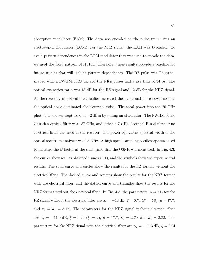
67
absorption modulator (EAM). The data was encoded on the pulse train using an
electro-optic modulator (EOM). For the NRZ signal, the EAM was bypassed. To
avoid pattern dependences in the EOM modulator that was used to encode the data,
we used the fixed pattern 01010101. Therefore, these results provide a baseline for
future studies that will include pattern dependences. The RZ pulse was Gaussian-
shaped with a FWHM of 23 ps, and the NRZ pulses had a rise time of 34 ps. The
optical extinction ratio was 18 dB for the RZ signal and 12 dB for the NRZ signal.
At the receiver, an optical preamplifier increased the signal and noise power so that
the optical noise dominated the electrical noise. The total power into the 20 GHz
photodetector was kept fixed at −2 dBm by tuning an attenuator. The FWHM of the
Gaussian optical filter was 187 GHz, and either a 7 GHz electrical Bessel filter or no
electrical filter was used in the receiver. The power-equivalent spectral width of the
optical spectrum analyzer was 25 GHz. A high-speed sampling oscilloscope was used
to measure the Q-factor at the same time that the OSNR was measured. In Fig. 4.3,
the curves show results obtained using (4.51), and the symbols show the experimental
results. The solid curve and circles show the results for the RZ format without the
electrical filter. The dashed curve and squares show the results for the NRZ format
with the electrical filter, and the dotted curve and triangles show the results for the
NRZ format without the electrical filter. In Fig. 4.3, the parameters in (4.51) for the
RZ signal without the electrical filter are αe = −18 dB, ξ = 0.74 (ξ ′ = 5.9), µ = 17.7,
and κ0 = κ1 = 3.17. The parameters for the NRZ signal without electrical filter
are αe = −11.9 dB, ξ = 0.24 (ξ ′ = 2), µ = 17.7, κ0 = 2.79, and κ1 = 2.82. The
parameters for the NRZ signal with the electrical filter are αe = −11.3 dB, ξ = 0.24
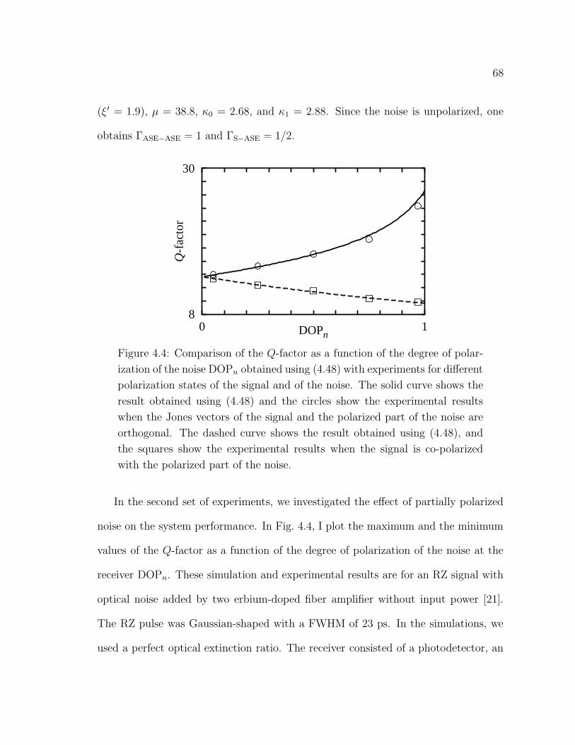
68
(ξ′ = 1.9), µ = 38.8, κ0 = 2.68, and κ1 = 2.88. Since the noise is unpolarized, one
obtains ΓASE−ASE = 1 and ΓS−ASE = 1/2.
8
30
0 1
Q-f
acto
r
DOPn
Figure 4.4: Comparison of the Q-factor as a function of the degree of polar-
ization of the noise DOPn obtained using (4.48) with experiments for different
polarization states of the signal and of the noise. The solid curve shows the
result obtained using (4.48) and the circles show the experimental results
when the Jones vectors of the signal and the polarized part of the noise are
orthogonal. The dashed curve shows the result obtained using (4.48), and
the squares show the experimental results when the signal is co-polarized
with the polarized part of the noise.
In the second set of experiments, we investigated the effect of partially polarized
noise on the system performance. In Fig. 4.4, I plot the maximum and the minimum
values of the Q-factor as a function of the degree of polarization of the noise at the
receiver DOPn. These simulation and experimental results are for an RZ signal with
optical noise added by two erbium-doped fiber amplifier without input power [21].
The RZ pulse was Gaussian-shaped with a FWHM of 23 ps. In the simulations, we
used a perfect optical extinction ratio. The receiver consisted of a photodetector, an
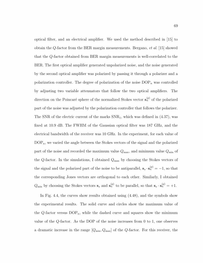
69
optical filter, and an electrical amplifier. We used the method described in [15] to
obtain the Q-factor from the BER margin measurements. Bergano, et al. [15] showed
that the Q-factor obtained from BER margin measurements is well-correlated to the
BER. The first optical amplifier generated unpolarized noise, and the noise generated
by the second optical amplifier was polarized by passing it through a polarizer and a
polarization controller. The degree of polarization of the noise DOPn was controlled
by adjusting two variable attenuators that follow the two optical amplifiers. The
direction on the Poincare sphere of the normalized Stokes vector s(p)n of the polarized
part of the noise was adjusted by the polarization controller that follows the polarizer.
The SNR of the electric current of the marks SNR1, which was defined in (4.37), was
fixed at 10.9 dB. The FWHM of the Gaussian optical filter was 187 GHz, and the
electrical bandwidth of the receiver was 10 GHz. In the experiment, for each value of
DOPn, we varied the angle between the Stokes vectors of the signal and the polarized
part of the noise and recorded the maximum value Qmax, and minimum value Qmin of
the Q-factor. In the simulations, I obtained Qmax by choosing the Stokes vectors of
the signal and the polarized part of the noise to be antiparallel, ss · s(p)n = −1, so that
the corresponding Jones vectors are orthogonal to each other. Similarly, I obtained
Qmin by choosing the Stokes vectors ss and s(p)n to be parallel, so that ss · s(p)
n = +1.
In Fig. 4.4, the curves show results obtained using (4.48), and the symbols show
the experimental results. The solid curve and circles show the maximum value of
the Q-factor versus DOPn, while the dashed curve and squares show the minimum
value of the Q-factor. As the DOP of the noise increases from 0 to 1, one observes
a dramatic increase in the range [Qmin, Qmax] of the Q-factor. For this receiver, the

70
parameters in (4.48) are µ = 38.6, κ1 = 1.7, κ0 = 0, and αe = 0. When the noise is
unpolarized (DOPn = 0), one has ΓASE−ASE = 1 and ΓS−ASE = 1/2. When the noise
is completely polarized (DOPn = 1), one has ΓASE−ASE = 1/2, so that ΓS−ASE = 1
when the noise is co-polarized with the signal and ΓS−ASE = 0 when the polarization
state of the noise is orthogonal to the signal. The results that I show in Figs. 4.2
and 4.4 illustrate the significant impact that partially polarized noise can have on
the performance of an optical fiber transmission system. Typical values for the PDL
per optical amplifier in optical fiber systems range from 0.1 dB to 0.2 dB [10], which
can partially polarize the optical noise in the transmission line. In a prototypical
trans-oceanic system described in [8], which has 270 amplifiers with 0.15 dB of PDL
per amplifier, the average noise DOP at the receiver is equal to 0.15. However, the
noise DOP in that trans-oceanic system exceeds 0.3 with a probability larger than
10−3.
4.5 Modulation format comparisons
In this section, I describe the use of (4.51) to compare the back-to-back performance
of three formats—CRZ, RZ, and NRZ—using the same receiver. To separate out
the effect of partially polarized noise from the modulation format in the system per-
formance, my colleagues and I only considered unpolarized noise in this study. We
found that the CRZ format outperforms both the RZ and the NRZ formats because
the CRZ format has a larger enhancement factor. We also found that the RZ format
outperforms the NRZ format for the same reason.

71
In Fig. 4.5, I use (4.51) to plot the Q-factor versus the OSNR for the CRZ, RZ,
and NRZ formats. The optical noise is unpolarized. The electric field of a CRZ pulse
is given by
es(t) =[
P0 cos2(πt/T )]1/2
exp [iAπ cos(2πt/T )] , (4.56)
where A = −0.6 is the chirp parameter, P0 is the peak power, and T is the bit
period [50]. To minimize the width of the pulses prior to the receiver, we transmitted
the CRZ signal through dispersive fiber with a total dispersion of −126 ps/nm [50]
in the simulations. The receiver consisted of a Gaussian-shaped optical filter with a
full-width at half maximum of 124 GHz and a fifth-order electrical Bessel filter with
a 3 dB spectral width of 8.5 GHz. The power-equivalent spectral width of the optical
spectrum analyzer was 50 GHz. The RZ pulse shape was determined by setting A = 0.
The rise time of an NRZ pulse was 30 ps. We compared the performance of these
formats using both a perfect extinction ratio and an optical extinction ratio of 18 dB.
With a finite extinction ratio, for the CRZ and the RZ formats we used the same
pulse shapes in the spaces as in the marks but with a lower power, while the NRZ
format was constructed by low-pass filtering a two-level step function. In Fig. 4.5, the
solid, dashed and dotted curves show the results for the CRZ, RZ, and NRZ formats
respectively, all with a perfect extinction ratio. The solid curve with circles, dashed
curve with squares, and dotted curve with triangles show the corresponding results
with an optical extinction ratio of 18 dB.
In Fig. 4.6, I compare the shapes of an isolated mark for the three formats prior
to the receiver. The solid, dashed and dotted curves are results for the CRZ, RZ, and
NRZ formats, respectively. The parameters used in (4.51) for the formats that my

72
4
11
3 15
Q-f
acto
r
OSNR
Figure 4.5: A performance comparison of the Q-factor as a function of the
OSNR for three modulation formats using (4.51). The parameters of the
formats are given in Table 4.1. The power-equivalent spectral width of the
optical spectrum analyzer was 50 GHz. The solid, dashed, and dotted curves
show the results for the CRZ, RZ and NRZ formats respectively, all with a
perfect extinction ratio. The solid curve with circles, the dashed curve with
squares, and the dotted curve with triangles show the corresponding results
with an optical extinction ratio of 18 dB.
colleagues and I simulated are shown in Table 4.1. The currents in the formula (4.38)
for the αe can be determined from the optical extinction ratio αo using (4.21). The
enhancement factor (4.50) is larger for the CRZ format than for the RZ format and
is larger for the RZ format than for the NRZ format, due to the decrease in the pulse
duration prior to the receiver, as shown in Fig. 4.6. Thus, for the results shown in
Fig. 4.5, and also for those in [20], the primary reason the RZ format has a better
back-to-back performance than the NRZ format using the same receiver is because
the RZ format has a larger enhancement factor ξ. For the same reason, the CRZ
format has a better performance than the RZ format. Fig. 4.5 shows a substantial
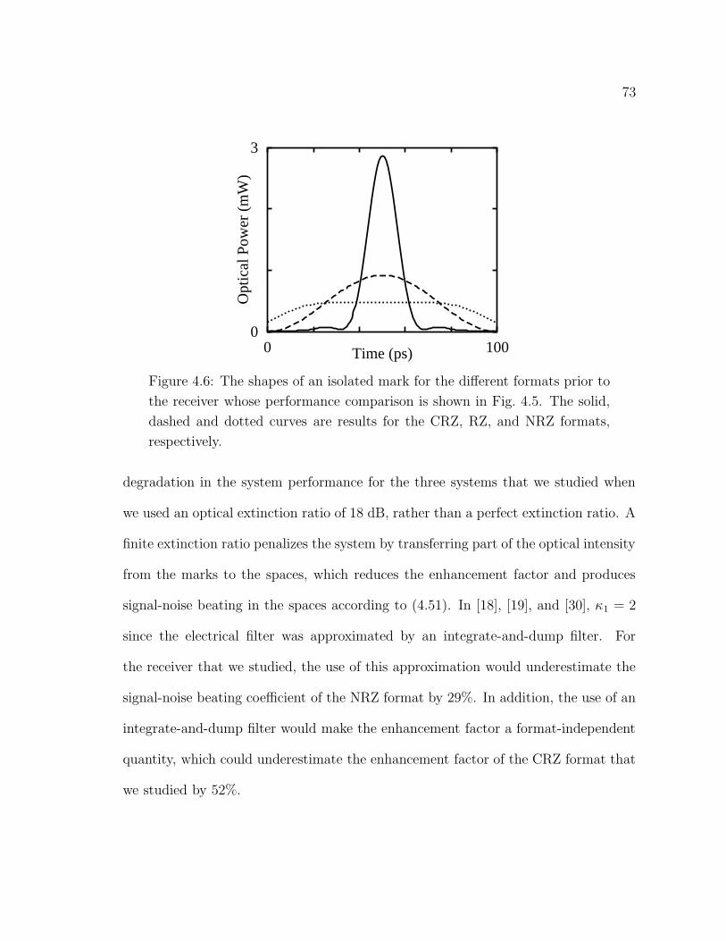
73
0
3
0 100
Opt
ical
Pow
er (
mW
)
Time (ps)
Figure 4.6: The shapes of an isolated mark for the different formats prior to
the receiver whose performance comparison is shown in Fig. 4.5. The solid,
dashed and dotted curves are results for the CRZ, RZ, and NRZ formats,
respectively.
degradation in the system performance for the three systems that we studied when
we used an optical extinction ratio of 18 dB, rather than a perfect extinction ratio. A
finite extinction ratio penalizes the system by transferring part of the optical intensity
from the marks to the spaces, which reduces the enhancement factor and produces
signal-noise beating in the spaces according to (4.51). In [18], [19], and [30], κ1 = 2
since the electrical filter was approximated by an integrate-and-dump filter. For
the receiver that we studied, the use of this approximation would underestimate the
signal-noise beating coefficient of the NRZ format by 29%. In addition, the use of an
integrate-and-dump filter would make the enhancement factor a format-independent
quantity, which could underestimate the enhancement factor of the CRZ format that
we studied by 52%.

74
Format αo (dB) ξ′ ξ K1 K0 M
CRZ −∞ 4.20 0.80 3.48 0 21.23
CRZ −18 4.13 0.78 3.48 2.99 21.23
RZ −∞ 3.21 0.61 3.05 0 21.23
RZ −18 3.16 0.60 3.05 3.04 21.23
NRZ −∞ 2.12 0.40 2.83 0 21.23
NRZ −18 2.05 0.39 2.83 2.74 21.23
Table 4.1: Parameters of the modulation formats used in Figs. 4.5 and 4.6.

Chapter 5
Importance sampling for the
polarization-induced penalty
5.1 Computation of outage probability
A major goal in the design of wavelength-division-multiplexed (WDM) optical fiber
communications systems is to minimize the probability of channel outages due to
polarization effects. System designers commonly allocate a prescribed margin to
polarization effects, such as 2 dB, with a fixed probability that the margin will be
exceeded, such as 10−5, corresponding to approximately five minutes per year. When
this margin is exceeded an outage is said to occur. Because outages are extremely
rare, it has been difficult to study them theoretically using standard Monte Carlo
simulations and experimentally using laboratory and field experiments.
Wang and Menyuk [8] proposed the reduced Stokes model as a tool to compute the
evolution of the optical signal-to-noise ratio (OSNR) and the polarization states of the
signal and noise for each channel in long-haul optical fiber communications systems,
which I described in Chapter 3. For a given fiber realization, one may calculate the
Q-factor from the OSNR and the polarization states of the signal and noise using
75

76
the receiver model that I introduced in Chapter 4. First, one computes the Q-factor
when PDL and PDG are present and when they are absent for a fixed level of PMD.
From that, one may determine the Q-penalty in dB due to these effects, where the
Q-penalty is defined to be the difference between the Q-factor in dB without PDL and
PDG and the Q-factor in dB when all the polarization effects are included. One then
defines the outage probability due to the polarization effects to be the probability
that the Q-penalty exceeds an allowed margin, such as 1 or 2 dB. This margin, which
is specified during the design of the system, determines the tolerance limit of the
operation of the system.
The reduced Stokes model decreases the computational time of simulations of the
polarization effects by several orders of magnitude when compared to a full time-
domain simulation. Even so, until now, efficient computation of outage probabilities
has only been carried out using numerical extrapolation with a Gaussian function [8]
to estimate the tails of the probability density function (pdf) of the Q-penalty. With
the collaboration of my colleagues, I developed an importance sampling technique
[51] to resolve the tails of the pdf of the Q-penalty and thereby efficiently compute
outage probabilities as small as 10−6 [16] using a fraction of the computational time
required by standard Monte Carlo simulations. In addition, we have been able to
determine the error that one can make in the computation of the Q-penalty when the
polarization states of the signal and noise are not accounted for in the receiver.
In Sec. 5.2, I present a validation of the reduced Stokes model that I described in
Chapter 3 in combination with the accurate receiver model that I derived in Chapter 4
by comparison to full time-domain simulations. In Sections 5.3 and 5.4, I show how

77
the probability of a rare event can be efficiently computed using Monte Carlo simu-
lations with an importance sampling technique that my colleagues and I developed.
Using this technique, one can compute outage probabilities using a small fraction of
the time required by standard Monte Carlo simulations. We validated this impor-
tance sampling technique by comparison with extensive Monte Carlo simulations. In
Sec. 5.5, I show how the outage probability due to the polarization effects depends
on the polarization-dependent loss (PDL) per optical amplifier, based on simulations
with the reduced Stokes model and the accurate receiver model. I also show the
relative variation in the results that we obtained using Monte Carlo simulations with
importance sampling.
5.2 Reduced Stokes model validation
In order to compute outage probabilities using the reduced Stokes model, my col-
leagues and I had to first validate the implementation of the reduced model by com-
parison to a full time-domain model using the Manakov-PMD equation [27] that I
described in Chapter 2. Figures 5.1(a) and 5.1(b) show numerical results of the mean
of the Q-penalty ∆Q in dB and its standard deviation, respectively, as a function of
the PDL per optical amplifier for the full and the reduced models. I define Q in dB
as QdB = 20 log10(Q), as in [15]. The system that we studied had eight 10 Gbit/s
return-to-zero channels spaced 1 nm (124 GHz) apart. The total propagation distance
was 8, 910 km, with an amplifier spacing of 33 km. Therefore, there were 270 optical
amplifiers in the system. The PDG was equal to 0.06 dB per optical amplifier. For
the full model, the fiber’s nonlinear coefficient n2 was 2.6 × 10⁻²⁰ m2/W, the fiber’s

78
effective area was 80 µm2, and the optical signal consisted of a string with 64 bits
obtained using the pseudo-random bit string (PRBS) algorithm [52]. The periodic
dispersion map consisted of one section of dispersion-shifted fiber whose dispersion
was −2 ps/nm-km at 1550 nm and whose length was 264 km, followed by a sec-
tion of single mode fiber whose dispersion was 16 ps/nm-km and whose length was
33 km. In both sections, the dispersion slope was equal to 0.07 ps/nm2-km. The
residual dispersion in each of the channels was compensated using symmetric pre-
and post-dispersion compensation. Since the full simulations require a large amount
of computer time, we only compared the mean and the standard deviation of the
Q-penalty, and we only used 20 random fiber realizations with the same mean DGD.
To compare the two models I used the same fiber realizations in both the full and the
reduced model simulations to avoid the statistical uncertainty in the computation of
the mean and the standard deviation of the Q-penalty. In addition, we used the same
set of fiber realizations for each PDL value. Therefore, the only uncertainty in the
comparison comes from the nonlinear polarization rotation in the full time-domain
simulations. In [8], a similar comparison was carried out, except that the receiver
model did not account for the polarization state of the noise in the receiver. There-
fore, the comparison in [8] was essentially a comparison of signal-to-noise ratios in
the two models, rather than a comparison of Q-factors. In addition, the random fiber
realizations used in the full and the reduced model were independently generated.
The use of different fiber realizations in the full and reduced models significantly con-
tributed to the uncertainty in the comparison. In Fig. 5.1, the agreement between the
full model and the reduced model with 20 Monte Carlo samples is good. The reduced

79
model slightly overestimates the standard deviation of the Q-penalty in Fig. 5.1, be-
cause the reduced model neglects the slight depolarization that a channel suffers due
to PMD. Consequently, with the reduced model, an entire channel can be aligned with
the high-loss axis of a PDL element, whereas that is not the case with the full model
since the channel will suffer some depolarization due to PMD. We did not compute
more than 20 Monte Carlo samples per PDL in the full model simulations because
the full model requires an extensive amount of computer time. When we increased
the number of realizations in the reduced model to 103, the agreement was still very
good.
My colleagues and I computed the Q-factor from the full time and frequency
domain model using the Manakov-PMD equation [27] in combination with a procedure
introduced in [20]. We used a step size of 0.5 km to numerically solve the Manakov-
PMD equation. In [20], the BER was computed by averaging the probability of errors
in all the marks and spaces of the bit string, since each bit in the string can suffer
significant nonlinear polarization rotation and, therefore, suffer a different impairment
due to the signal-noise beating. Using the Gaussian approximation, the BER in a
string with N0 spaces and N1 marks sampled with the sampling time offset ts is given
by
BER(ts, ith) =1
N0
N0+N1∑
j=1
I0(ts + jT ) erfc
[
ith − i(ts + jT ) − 〈in〉√2σi(ts + jT )
]
+1
N1
N0+N1∑
j=1
I1(ts + jT ) erfc
[
i(ts + jT ) + 〈in〉 − ith√2σi(ts + jT )
]
,
(5.1)

80
0
1.0
⟨∆Q
⟩ (dB
)
(a)
0
1.2
0 0.3
σ ∆Q
(dB
)
PDL (dB)
(b)
Figure 5.1: Validation of the reduced Stokes model. I show the (a) mean and
(b) standard deviation of the Q-penalty ∆Q in dB as a function of the PDL
per optical amplifier. The dotted lines are results of full model simulations
with 20 samples of fiber realizations. The dashed lines are results of reduced
model simulations with 20 samples. The solid lines are results of reduced
model simulations with 103 samples.
where 〈in〉 and σi(t) are respectively the mean and the instantaneous standard devia-
tion of the electric current due to optical noise, which were defined in (4.22) and (4.23),
respectively. The function I0(t) is 1 if the bit is a space and 0 otherwise. The func-
tion I1(t) is given by 1 − I0(t). The bit period T is equal to 100 ps. To determine
the sampling time for marks and spaces, we used the clock recovery algorithm that I
described in Sec. 4.2.4. Using (5.1), we determined the decision threshold ith as the

81
value that minimizes the BER, which we computed using a zero-finding algorithm.
Once the BER was obtained, we computed the corresponding Q-factor by solving the
transcendental equation that relates the Q-factor to the BER,
BER =1
2erfc
(
Q√2
)
. (5.2)
Since the term on the right-hand side of (5.2) varies exponentially with Q, we solved Q
for a given BER by computing the logarithm of the terms in each side of this equation.
Therefore, we computed the Q-factor by searching for the root of the equation
log10 (BER) − log10
[
1
2erfc
(
Q√2
)]
= 0 (5.3)
using Brent’s root search method [53].
5.3 Importance sampling
Importance sampling is a well known technique in statistics that makes a more efficient
use of Monte Carlo simulations to compute the probability of rare events. For the
problem of computing the outage probability due to the polarization effects for a given
channel in a WDM system, the rare events that interest us are those for which the Q-
penalty is close to the allowed margin in a given channel. This value is typically large
compared to the average or expected value of the Q-penalty. To successfully apply
importance sampling to this problem, one needs some knowledge of which random
realizations of the fiber PMD produce these large Q-penalties. These random fiber
realizations are those for which the Stokes vector of the signal in a given channel is
more likely to be aligned with the high-loss axes of the PDL elements than with the
low-loss axes.

82
The basic idea of Monte Carlo simulations with importance sampling is to bias
the pdfs of the sources of randomness so that the rare events of interest occur more
frequently than they would in standard Monte Carlo simulations and then to weight
the samples by the likelihood that the biased random quantities would actually appear
in standard Monte Carlo simulations. My colleagues and I observed that the use of
a single biased distribution with importance sampling is insufficient to resolve the
histogram of the penalty produced by the polarization effects in the configuration
space. Thus, it is necessary to combine the statistical results from several biased
distributions, since each distribution statistically resolves a different region in the
configuration space. However, the biased distributions that do not statistically resolve
a given region in the configuration space can significantly degrade the accuracy of the
estimation of the probability in that region if they are inadequately combined with
the other distributions. This effect is particularly evident in the computation of the
penalty because the angles between the polarization state of the channel and the
high-loss axes of the PDL elements in each amplifier that we bias are not the only
quantities that determine the penalty. The direction of the normalized Stokes vectors
of the signal in other channels throughout the transmission line and the angle between
the normalized Stokes vector of the signal and the normalized Stokes vector of the
polarized part of the noise in a given channel at the receiver also influence the penalty.
Using importance sampling, the probability PI of an event defined by the indicator
function I(x), whose value is either 0 or 1, can be mathematically expressed by [54]
PI =
J∑
j=1
1
Mj
Mj∑
i=1
I(xj,i)wj(xj,i)Lj(xj,i), (5.4)

83
where
Lj(xj,i) =p(xj,i)
p∗j(xj,i)(5.5)
is the likelihood ratio of the i-th sample xj,i drawn from the j-th biased distribution,
and Mj is the number of samples drawn from the j-th biased distribution p∗j(x).
The term p(x) is the pdf of the j-th unbiased distribution, and J is the number of
different biased distributions. The weights wj(x) allow one to combine different biased
distributions. In this application, the random vector x corresponds to the random
realization of the fiber PMD, which is determined by the random mode coupling
transformations between the birefringent sections, and the unbiased pdf is known a
priori. The indicator function I is chosen to compute the probability of having the
Q-penalty within a given range, such as a bin in a histogram.
An efficient technique to combine the samples from multiple biased distributions
is the balanced heuristic method [54], which my colleagues and I used for the work
reported in this dissertation. The balanced heuristic weight assigned to the sample x
drawn from the j-th distribution is given by
wj (x) =MjL
−1j (x)
∑Jk=1MkL
−1k (x)
. (5.6)
The idea behind the balanced heuristic method is that samples are weighted accord-
ing to the likelihood that each biased distribution produces samples in that region;
distributions that are more likely to put samples there are weighted more heavily.
The computation of the balanced heuristic weight for any given sample requires that
the likelihood ratio of all the biased distributions be evaluated for that sample. In
other words, the likelihood ratio of all J biased distributions have to be evaluated

84
for the i-th sample drawn from the j-th distribution, even though this sample was
obtained using only the biased pdf of the j-th distribution.
A confidence interval for the estimator of the probability PI of the indicator func-
tion I(x) in (5.4) can be defined from the estimator of the variance of PI , which is
given by
σ2PI
=
J∑
j=1
1
Mj (Mj − 1)
Mj∑
i=1
[
I(xj,i)wj(xj,i)Lj(xj,i) − PIj
]2
, (5.7)
where
PIj=
1
Mj
Mj∑
i=1
I(xj,i)wj(xj,i)Lj(xj,i), (5.8)
is the contribution of the samples drawn from j-th biased distribution to the esti-
mator PI. The confidence interval of the estimator PI is defined to be the interval(
PI − σPI, PI + σPI
)
. The relative variation equals σPI/PI. The key to the derivation
of (5.7), which we will present in [55], was to realize that the product between the in-
dicator function I(x) and its corresponding weight wj(x)L(x) is the random variable
in the standard expression of the variance [49] for the j-th distribution. Then, the
variances produced by all the independent biased distributions are added to obtain
the expression for the variance of the estimator PI in (5.7).
5.4 Importance sampling for the polarization-in-
duced penalty
The key issue in applying importance sampling is to choose the biased pdf p∗(x). In
the reduced model, the PDL is lumped in the optical amplifiers. So, to compute the

85
s 1
s 3
s 2
s PDL
R PMD s channel
θ n
Figure 5.2: Poincare sphere with the diagram of the importance sampling
technique for the PDL-induced penalty. The vector RPMD schannel is the nor-
malized Stokes vector of a given channel prior to the n-th PDL element, sPDL
is the normalized Stokes vector that is parallel to the high-loss axis of the
n-th PDL element, and θn is the angle between these two vectors, which I
bias towards zero.
outage probability for a given channel, the appropriate pdfs to bias are the pdfs of the
angles θn between the polarization state of the channel and the polarization state that
undergoes the highest loss due to PDL in the n-th optical amplifier. This procedure
is illustrated in Fig 5.2, where the polarization transformation matrix RPMD of the
last birefringent section of the fiber is biased so that the transformed polarization
state of a given channel RPMD schannel is more likely to be aligned to the high-loss axis
sPDL of the PDL elements in each of the optical amplifiers along the transmission. I
stress that the method is self-validating. If one biases the samples incorrectly, then

86
the variance of the results is large.1 By biasing cos θn towards one, one increases the
likelihood that the Q-penalty of the channel will be large. The angles θn are directly
determined by the realization of the random mode coupling in the last birefringent
section of the fiber that precedes the n-th optical amplifier. Thus, the values of
cos θn play the role of the components of the random vector x in (5.4). In standard
Monte Carlo simulations, in which the PMD is modeled using the coarse step method
[27], the cosines of each of the angles θn are uniformly distributed in the interval
[−1, 1]. One can note that an unbiased importance sampling simulation, for which
L(x) = 1, is exactly the same as a standard Monte Carlo simulation. However, in
biased importance sampling one fixes a biasing parameter α and selects the cos θn
from a biased pdf, p∗α(cos θ). In the work reported in this dissertation, my colleagues
and I used the biased pdf
p∗α (cos θ) =α
1 − e−2αe−α(1−cos θ), (5.9)
which biases cos θ towards 1 when α is positive and which corresponds to standard
Monte Carlo simulations in the limit α = 0. The likelihood ratio for this pdf is given
by
Lα (cos θ) =1 − e−2α
2αeα(1−cos θ). (5.10)
Since the unbiased cos θn are independent random variables, the likelihood ratio for
a biased realization of the fiber PMD is equal to the product of the likelihood ratios
for each of its biased angles. The actual pdf of the Q-penalty is obtained using (5.4)
1There is one important caveat: If two or more disconnected regions in the phase space produce
the same penalty, then it is possible in principle to have low variance and for the result to still be
incorrect. This outcome does not appear to be physically possible for the problem studied here.

87
by weighting each fiber sample by its likelihood ratio, which is the likelihood that the
biased fiber realization would actually occur in an unbiased simulation. By using the
balanced heuristic method to combine several Monte Carlo simulations with different
values of the biasing parameter α, one can statistically resolve the pdf of theQ-penalty
in any desired range.
To use importance sampling, one must determine the value of the biasing param-
eter α that enables one to statistically resolve the histogram of the Q-penalty over a
range of Q-penalty values whose probability is on the order of a given target proba-
bility Pα, such as Pα = 10−6. My colleagues and I observed that a biased distribution
efficiently resolves the probability of a given bin in the histogram of the Q-penalty
when the indicator function for this bin has the value 1 for a large proportion of
the biased samples. Therefore, the required value of the biasing parameter α is the
one for which the target probability Pα is equal to the likelihood ratio of the biased
realization of the fiber PMD evaluated at the expected value of the random variable
cos θ with biased pdf p∗α. That is, the bias parameter α satisfies the equation
Pα = LNα [〈cos θ〉] = LN
α
(
1 + e−2α
1 − e−2α− 1
α
)
, (5.11)
where N is the number of optical amplifiers, and 〈·〉 is the expectation operator. For
example, P0.3 = 1.5 × 10⁻² and P0.6 = 1.8 × 10⁻⁷ for N = 80. In Fig. 5.3, I show the
pdf of cos θ for α = 0, which produces unbiased samples, together with α = 0.3 and
α = 0.6. Just as in a standard Monte Carlo simulation, as one increases the number
of samples with the bias parameter α, one increases the size of the interval about Pα
for which the histogram of the Q-penalty is well resolved.

88
0
1
-1 1
cos θ
Figure 5.3: Biased pdf of cos θ defined in (5.9) for different values of bias
strength α. The solid curve shows results for α = 0, which corresponds to
the unbiased pdf. The dashed curve shows results for α = 0.3. The dotted
curve shows results for α = 0.6.
For the importance sampling technique to be efficient it is required that the per-
formance measure, the Q-penalty, be highly correlated with the random variables
that are being biased, the values of cos θn. In other words, given a set of random
values of cos θn, a perturbation in any of the values of cos θn towards 1 should always
produce an increase in the Q-penalty. If this requirement is not met, the statistical
uncertainty of the results may be so large that importance sampling provides little
or no improvement over standard Monte Carlo simulations. For a single channel sys-
tem with PMD and PDL, small values of the angles θn are very highly correlated
to large Q penalties. Moreover, the effect of adding gain saturation and PDG to
such a system is to always increase the Q-penalty. Consequently, my colleagues and I
found that importance sampling is efficient for single channel simulations. However,
in a WDM system, the Q-penalty for a given channel also depends on the angles

89
the polarization states of the other channels make with the polarization state with
highest loss due to PDL, as can be illustrated by the following two extreme cases:
I consider a given channel, whose polarization state is aligned with the polarization
state with highest loss due to PDL. In the first case, I suppose that the polarization
states of the other channels are all aligned with the polarization state with lowest
loss due to PDL, so that when the total power is partially restored by each of the
gain-saturated amplifiers, the given channel loses power relative to the other channels
and the largest possible Q-penalty is incurred. In the second case, I suppose that all
the channels are co-polarized, so that the given channel does not transfer any power
to the other channels and therefore incurs a much smaller Q-penalty. When PDG is
included, the variation in the Q-penalty can be even larger for a fixed set of biasing
angles θn, since in this case the penalty also depends on the degree of polarization
(DOP) and on the total polarization state. Therefore, in a WDM system with only
a few channels, the correlation between the Q-penalty and the angles θn is not as
high as in the single channel system and the importance sampling procedure that I
described is not as efficient. On the other hand, since PMD tends to randomize the
polarization states of the channels, one finds that as the number of channels increases
the DOP decreases. Thus, the Q-penalty becomes less dependent on the polarization
states of the other channels and on the PDG, and the importance sampling procedure
becomes more efficient. In the next section, I will show that this procedure is highly
efficient for a WDM system with as few as eight channels.

90
5.5 Numerical results
In this section, I describe the outage probabilities due to polarization effects for a
trans-oceanic WDM system by applying importance sampling to resolve the tails
of the pdf of the Q-penalty for the same system that I presented in Sec. 5.2. My
colleagues and I validated the method of computing outage probabilities using Monte
Carlo simulations with importance sampling by making comparisons with extensive
standard Monte Carlo simulations. To obtain these results, we used the reduced model
that I described in Chapter 3 and the receiver model that I described in Chapter 4.
For the results in this chapter, we obtained the final histograms of the Q-penalty by
dividing the range of penalties in dB into 50 bins and by combining all the biased
distributions using the balanced heuristic method that I described in Sec. 5.3.
We simulated a 10 Gbit/s return-to-zero (RZ) system with eight WDM channels
spaced 1 nm (124 GHz) apart. The total propagation distance was 8, 910 km and
the amplifier spacing was 33 km. The PMD was 0.1 ps/km1/2. In Fig. 5.4, I plot
the outage probability as a function of the allowed Q-penalty margin ∆Q. The PDL
was 0.13 dB and the PDG was 0.06 dB per optical amplifier. The solid curve shows
the outage probability that is computed using 104 Monte Carlo simulations with
importance sampling for each biased distribution pα(·) in (5.9) with: α = 0, which
corresponds to unbiased simulations, α = 0.3, α = 0.4, α = 0.5 and α = 0.6. In
Fig. 5.4, a dashed curve shows results of extensive Monte Carlo simulations with a
total of 5 × 10⁶ samples. The agreement with the importance sampling results is
good up to outage probability at which we could obtain in a statistically significant

91
100
10-9
0 4
Out
age
prob
abili
ty
∆Q (dB)
Figure 5.4: The outage probability as a function of the allowed Q-penalty
margin ∆Q in dB for an eight channel WDM system. We set PDL = 0.13 dB
and PDG = 0.06 dB per optical amplifier. The solid curve shows results of
5 × 10⁴ Monte Carlo simulations with importance sampling. The dashed
curve shows results of 5×10⁶ standard Monte Carlo simulations. The dotted
curve shows results obtained with the same 5× 10⁴ Monte Carlo simulations
with importance sampling, but assuming that the noise is always unpolarized
at the receiver.
number of samples. We used the same computer and the same program for both the
extensive Monte Carlo simulations and the simulations with importance sampling;
the only difference is that we did not bias the fiber birefringence for the standard
Monte Carlo method. The results with importance sampling required only 1% of
the computational time that was required by extensive Monte Carlo simulations.
The dotted curve shows the outage probability obtained with the same Monte Carlo
simulations with importance sampling, but using the receiver model that assumes
unpolarized noise in the receiver. As a consequence, this model implicitly assumes
that half of the noise beats with the signal in the photodetector, which leads to

92
incorrect results. Thus, we conclude that it is very important to properly account for
the polarization states of the signal and the noise in the receiver.
In Fig. 5.5, I plot the outage probability at margins of 1 dB and 2 dB as a function
of the PDL per optical amplifier for the same system as in Fig. 5.4. For these results,
my colleagues and I used Monte Carlo simulations with importance sampling. The
solid curve with circles shows that the PDL per optical amplifier must not exceed
0.11 dB in order for the probability that the Q-penalty exceeds 2 dB be smaller that
10−6. Therefore, if the margin allocated in the design to the penalty produced by
the polarization effects is equal to 2 dB with an outage probability of 10−6, the PDL
per optical amplifier must not be larger than 0.11 dB. If the margin allocated to the
polarization effects is equal to 3 dB, shown with a dashed line with diamonds, the
PDL per optical amplifier can be as large as 0.15 dB with an outage probability of
10−6.

93
100
10-10
0 0.25
Out
age
Prob
abili
ty
PDL (dB)
Figure 5.5: The outage probability as a function of the PDL per optical
amplifier for two Q-penalty margins ∆Q. The solid curve with circles shows
the probability that the Q-penalty exceeds 2 dB. The dashed curve with
diamonds shows the probability that the Q-penalty exceeds 3 dB. The error
bars show the confidence interval for the curves computed using (5.7). Thedotted line shows the 10−6 outage probability level.

Chapter 6
Fiber recirculating loop experiments
6.1 Fiber recirculating loops
Optical fiber recirculating loops are useful tools for laboratory studies of the effects
that limit the performance of optical fiber communications systems [5]. In this chap-
ter, I present an experimental validation of the reduced Stokes model that I described
in Chapter 3 in combination with the receiver model that I derived in Chapter 4 by
comparison with dispersion-managed soliton, optical-fiber recirculating loop experi-
ments.
The evolution of the polarization states in fiber recirculating loops is periodic,
which contrasts with the random evolution of the polarization states due to PMD
in straight-line systems. As a consequence of this periodicity, polarization effects
accumulate faster in fiber recirculating loops than in straight-line systems [56], [57].
To overcome this problem, my colleagues and I use a loop-synchronous polariza-
tion scrambler in both sets of experiments that I describe in this chapter. Loop-
synchronous polarization scramblers are used to rotate the polarization state of the
signal after each round trip of the loop to emulate PMD-induced polarization rota-
94

95
tions and, thereby, to break the periodicity of the evolution of the polarization states
during the transmission [56]. In this set of fiber recirculating loop experiments, which
was carried out primarily by Yu Sun at the University of Maryland Baltimore County,
we showed that partially polarized noise due to PDL causes an asymmetrical Q-factor
distribution in the receiver. We also showed that it is very important to account for
the polarization state of the noise at the receiver when computing the performance
of fiber recirculating loop systems.
6.2 Experimental Q-factor distribution
In this section, I show that partially polarized noise due to PDL causes an asym-
metrical Q-factor distribution at the receiver. This asymmetry occurs because the
SNR of the electrical current in the receiver does not completely determine the Q-
factor if the noise is partially polarized. Therefore, it is very important to accurately
model the contribution of the partially polarized noise at the receiver as I described
in Chapter 4.
In Fig 6.1, I show a diagram of the optical fiber recirculating loop that my col-
leagues and I used. This fiber recirculating loop was a dispersion-managed soli-
ton (DMS) system that consisted of 100 km of dispersion-shifted fiber with D =
−1 ps/nm-km, followed by 7 km of single-mode fiber with D = 17 ps/nm-km. We
used a LiNbO3 polarization controller to synchronously scramble the polarization
state of the light in the loop once per round trip, which we controlled using a pro-
grammable waveform generator. The PDG was equal to 0.05 dB per optical amplifier
and the PMD was equal to 0.1 ps/km1/2. The PDL per round trip could be varied

96
T X
AO switch
AO switch
R X
LiNbO 3
25 km DSF
EDFA
25 km DSF
WFG
3 dB
OF 2.8 nm
3.5 km SMF
25 km DSF
3.5 km SMF
25 km DSF
EDFA
EDFA
EDFA
EDFA
PC
PC
Figure 6.1: Diagram of the fiber recirculating loop experiment.
from 0.13 dB to 0.6 dB by adjusting the manual polarization controllers inside the
loop. In the DMS loop, the interaction between dispersion and nonlinearity produces
optical pulses that can be transmitted over ultra-long distances without suffering
waveform distortions even in the presence of intra-channel PMD [13], [58]. We prop-
agated a 10 Gbit/s return-to-zero (RZ) modulation format through 94 round trips to
emulate a long-haul undersea system with a total propagation distance of 10, 000 km.
We also employed a polarization scrambler at the transmitter to reduce the effect
of PDG. We chose a slow scrambling rate of 12.6 GHz to simultaneously reduce the
effects of PDG and the amplitude modulation induced by PDL [14].
In Fig. 6.2, I show the pdf of the Q-factor for the DMS fiber recirculating loop that
I showed in Fig. 6.1 with a PDL per round trip of 0.6 dB [22]. In Fig. 6.2, the dotted
bars are experimental results. The solid curve shows the result obtained from Monte
Carlo simulations using the reduced Stokes model with the accurate receiver model
that accounts for the polarization state of the noise at the receiver. The dashed
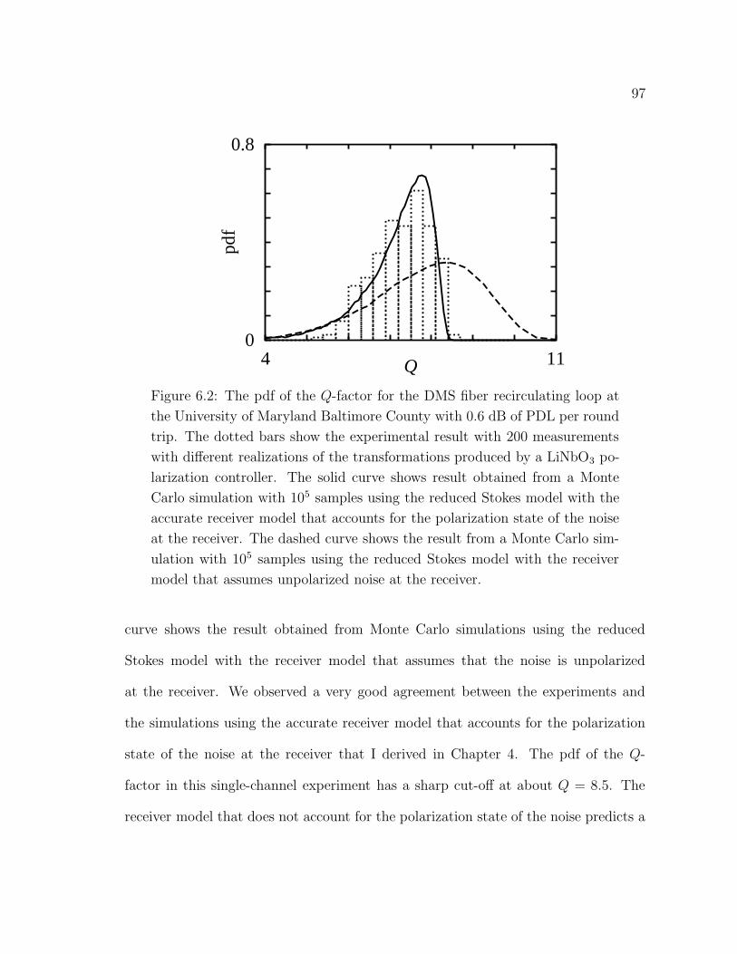
97
0
0.8
4 11
Q
Figure 6.2: The pdf of the Q-factor for the DMS fiber recirculating loop at
the University of Maryland Baltimore County with 0.6 dB of PDL per round
trip. The dotted bars show the experimental result with 200 measurements
with different realizations of the transformations produced by a LiNbO3 po-
larization controller. The solid curve shows result obtained from a Monte
Carlo simulation with 105 samples using the reduced Stokes model with the
accurate receiver model that accounts for the polarization state of the noise
at the receiver. The dashed curve shows the result from a Monte Carlo sim-
ulation with 105 samples using the reduced Stokes model with the receiver
model that assumes unpolarized noise at the receiver.
curve shows the result obtained from Monte Carlo simulations using the reduced
Stokes model with the receiver model that assumes that the noise is unpolarized
at the receiver. We observed a very good agreement between the experiments and
the simulations using the accurate receiver model that accounts for the polarization
state of the noise at the receiver that I derived in Chapter 4. The pdf of the Q-
factor in this single-channel experiment has a sharp cut-off at about Q = 8.5. The
receiver model that does not account for the polarization state of the noise predicts a

98
substantially larger tail for the large Q values. These large Q values were not observed
in the experiment because they come from realizations of the LiNbO3 polarization
controller that preferentially attenuate the noise that is in the polarization state
orthogonal to the polarization state of the signal. In this case, the optical noise at
the receiver is primarily co-polarized with the signal, which produces a variance of the
current due to the signal-noise beating that is equal to what would be produced in the
presence of an arbitrarily large noise component in the polarization state orthogonal
to the polarization state of the signal. Therefore, the receiver model that does not
account for the polarization state of the noise incorrectly assumes that half of the
optical intensity of the received noise produces signal-noise beating. The use of this
approximation significantly overestimates the probability of obtaining large Q values
for the same reason that it overestimates the penalty due to the polarization effects—
the probability of obtaining low Q values—as I showed in Chapter 5.

Chapter 7
Conclusions
Polarization effects can significantly limit the performance of long-haul terrestrial and
trans-oceanic optical fiber communications systems. Polarization effects can produce
randomly varying signal distortions and power penalties that can lead to system out-
ages on a time scale that varies between milliseconds and hours. Therefore, accurately
computing the penalty produced by the polarization effects is crucial in the design
of long-haul optical fiber communications systems. Wang and Menyuk [8] proposed
the reduced Stokes model as a tool for the computation of the penalty produced by
the polarization effects that is much more efficient than using the full time-domain
model. Even so, it is not currently feasible to accurately compute outage probabili-
ties as low as 10−6 using standard Monte Carlo simulations with the reduced Stokes
model. Moreover, the receiver model used by Wang and Menyuk did not account for
the effect of partially polarized noise in the receiver.
In this dissertation, I have described two contributions that I made with the
collaboration of my colleagues to the field of optical fiber communications systems.
These contributions extend and substantially improve the accuracy of the reduced
99

100
Stokes model. I described a technique that uses Monte Carlo simulations with im-
portance sampling that we developed to compute the probability density function
of the Q-factor and the outage probability for a channel in a long-haul, wavelength-
division-multiplexed optical fiber communications system due to the combination
of inter-channel polarization mode dispersion (PMD), polarization-dependent loss
(PDL), and polarization-dependent gain (PDG). This technique allows one to accu-
rately compute outage probabilities as small as 10−6 using the reduced Stokes model
at a fraction of the computational cost required by standard Monte Carlo simulations.
This technique was validated by comparison to extensive Monte Carlo simulations.
I also described an accurate formula that we developed that relates the Q-factor to
the OSNR for amplitude-shift-keyed optical fiber communication systems with arbi-
trary optical pulse shapes, arbitrary receiver characteristics and arbitrarily polarized
noise using an accurate receiver model. Using this formula, we showed how the per-
formance of a system depends on the state of polarization of the noise, which can
be significantly affected by PMD in the optical fiber, PDL, and PDG in the opti-
cal amplifiers. We also defined the enhancement factor and three other parameters
that explicitly quantify the performance of different modulation formats, which can
be useful in receiver optimization studies. We validated this formula by comparison
to back-to-back 10 Gbit/s experiments and Monte Carlo simulations. We also val-
idated the receiver model that I developed in combination with the reduced Stokes
model by comparison to optical fiber recirculating loop experiments. We applied
the proposed receiver model to compare the performance of the chirped return-to-
zero (CRZ), return-to-zero (RZ), and nonreturn-to-zero (NRZ) modulation formats

101
with a finite extinction ratio. We observed that the CRZ modulation format outper-
forms both the RZ and the NRZ formats with the same optical power and receiver
characteristics because the CRZ format has the largest enhancement factor for the
receiver that we studied. This method should be applicable to the study of other
amplitude-shift-keyed formats.
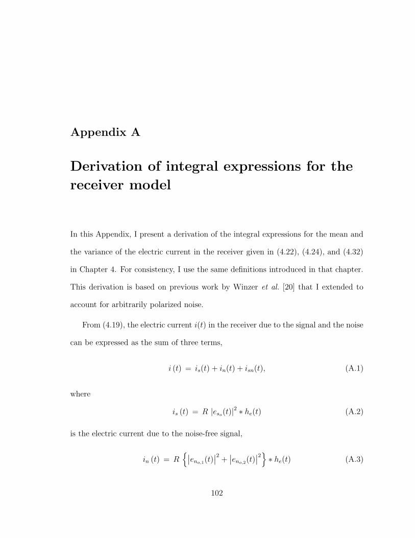
Appendix A
Derivation of integral expressions for the
receiver model
In this Appendix, I present a derivation of the integral expressions for the mean and
the variance of the electric current in the receiver given in (4.22), (4.24), and (4.32)
in Chapter 4. For consistency, I use the same definitions introduced in that chapter.
This derivation is based on previous work by Winzer et al. [20] that I extended to
account for arbitrarily polarized noise.
From (4.19), the electric current i(t) in the receiver due to the signal and the noise
can be expressed as the sum of three terms,
i (t) = is(t) + in(t) + isn(t), (A.1)
where
is (t) = R |eso(t)|2 ∗ he(t) (A.2)
is the electric current due to the noise-free signal,
in (t) = R{
∣
∣eno,1(t)
∣
∣
2+
∣
∣eno,2(t)
∣
∣
2}
∗ he(t) (A.3)
102
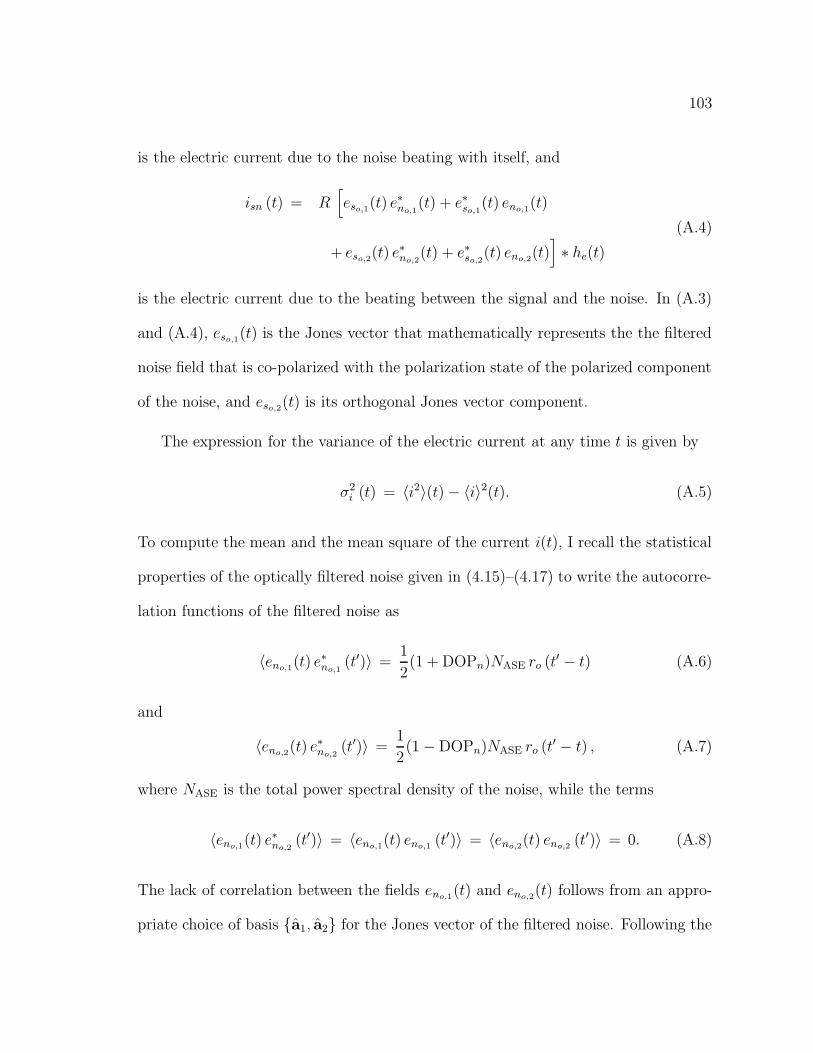
103
is the electric current due to the noise beating with itself, and
isn (t) = R[
eso,1(t) e∗no,1
(t) + e∗so,1(t) eno,1
(t)
+ eso,2(t) e∗no,2
(t) + e∗so,2(t) eno,2
(t)]
∗ he(t)
(A.4)
is the electric current due to the beating between the signal and the noise. In (A.3)
and (A.4), eso,1(t) is the Jones vector that mathematically represents the the filtered
noise field that is co-polarized with the polarization state of the polarized component
of the noise, and eso,2(t) is its orthogonal Jones vector component.
The expression for the variance of the electric current at any time t is given by
σ2i (t) = 〈i2〉(t) − 〈i〉2(t). (A.5)
To compute the mean and the mean square of the current i(t), I recall the statistical
properties of the optically filtered noise given in (4.15)–(4.17) to write the autocorre-
lation functions of the filtered noise as
〈eno,1(t) e∗no,1
(t′)〉 =1
2(1 + DOPn)NASE ro (t′ − t) (A.6)
and
〈eno,2(t) e∗no,2
(t′)〉 =1
2(1 − DOPn)NASE ro (t′ − t) , (A.7)
where NASE is the total power spectral density of the noise, while the terms
〈eno,1(t) e∗no,2
(t′)〉 = 〈eno,1(t) eno,1
(t′)〉 = 〈eno,2(t) eno,2
(t′)〉 = 0. (A.8)
The lack of correlation between the fields eno,1(t) and eno,2
(t) follows from an appro-
priate choice of basis {a1, a2} for the Jones vector of the filtered noise. Following the

104
same procedure used in the derivation of (A.6) and (A.7), I find that
〈eno,1(ti) e∗no,1
(tii) eno,1(tiii) e∗no,1
(tiv)〉 =1
4(1 + DOPn)
2N2ASE
×[
ro(tii − ti) ro(t
iv − tiii) + ro(tiv − ti) ro(t
iii − tii)]
,
(A.9)
and
〈eno,2(ti) e∗no,2
(tii) eno,2(tiii) e∗no,2
(tiv)〉 =1
4(1 − DOPn)2N2
ASE
×[
ro(tii − ti) ro(t
iv − tiii) + ro(tiv − ti) ro(t
iii − tii)]
.
(A.10)
Using (A.1) and (A.6)–(A.8), I find that the mean value of the current is given by
〈i〉(t) = is(t) + 〈in〉(t), (A.11)
which implies that
〈i〉2(t) = i2s(t) + 2 is(t) 〈in〉(t) + 〈in〉2(t) (A.12)
and
〈i2〉(t) = i2s(t) + 〈i2n〉(t) + 〈i2sn〉(t) + 2 is(t) 〈in〉(t). (A.13)
In (A.13), I do not include the terms that are proportional to 〈isn〉(t) because 〈isn〉(t)
averages out to zero, since the optical noise field has zero mean. Therefore, I can
express the variance of the current in the receiver as
σ2i (t) = σ2
ASE−ASE(t) + σ2S−ASE(t), (A.14)
where
σ2ASE−ASE(t) = 〈i2n〉(t) − 〈in〉2(t) (A.15)

105
is the variance of the current due to the noise-noise beating, and
σ2S−ASE(t) = 〈i2sn〉(t) (A.16)
is the variance of the current due to signal-noise beating.
To obtain closed form integral expressions for the mean and the variance of the
electric current due to noise in (A.15) and (A.16), respectively, I use the statistical
properties of the noise that I described in (A.6)–(A.10). The convolution of two
arbitrary functions g(t) and h(t) is defined by
g(t) ∗ h(t) =
∫ +∞
−∞
g(τ)h(t− τ)dτ. (A.17)
The limits of all of the integral expressions in this Appendix are from −∞ to +∞,
which for simplicity I suppress in all the subsequent expressions. Substituting (A.17)
into (A.3), I obtain
〈in〉(t) = R
∫
dti∫
dtii∫
dtiii〈en1(ti) e∗n1
(tii) 〉 ho(tiii − ti) h∗o(t
iii − tii) he(t− tiii)
+R
∫
dti∫
dtii∫
dtiii〈en2(ti) e∗n2
(tii) 〉 ho(tiii − ti) h∗o(t
iii − tii) he(t− tiii).
(A.18)
Substituting (A.6) and (A.7) into (A.18), I find that
〈in〉 = RNASE
∫
∣
∣ho(ti)∣
∣
2dti
∫
he(tii)dtii. (A.19)
Equation (A.19) can be further simplified to
〈in〉 = RNASEBo, (A.20)

106
where I define the electrical and the optical filter transfer functions such that |He(0)| =
|Ho(0)| = 1. Therefore, Bo = ro(0) =∫
|ho(τ)|2dτ is the power-equivalent spectral
width [24] of the optical filter.
Using (A.3), I can express the mean square of in(t) as
〈i2n〉(t) = 〈i2n1〉(t) + 〈i2n2
〉(t) + 〈i2n12〉(t), (A.21)
where
〈i2n1〉(t) =
⟨
[
R∣
∣eno,1(t)
∣
∣
2 ∗ he(t)]2
⟩
, (A.22)
〈i2n2〉(t) =
⟨
[
R∣
∣eno,2(t)
∣
∣
2 ∗ he(t)]2
⟩
, (A.23)
and
〈i2n12〉(t) = 2
⟨[
R∣
∣eno,1(t)
∣
∣
2 ∗ he(t)] [
R∣
∣eno,2(t)
∣
∣
2 ∗ he(t)]⟩
. (A.24)
Substituting (A.17) into (A.22)–(A.24), I obtain
〈i2n1〉(t) = R2
∫
dti∫
dtii∫
dtiii∫
dtiv∫
dtv∫
dtvi 〈en1(ti) e∗n1
(tii) en1(tiv) e∗n1
(tv)〉
×ho(tiii − ti) h∗o(t
iii − tii) ho(tvi − tiv) h∗o(t
vi − tv) he(t− tiii) he(t− tvi),
(A.25)
and 〈i2n2〉(t), which is the same as (A.25) when one replaces en1
(t) by en2(t), and
〈i2n12〉(t) = 2R2
∫
dti∫
dtii∫
dtiii∫
dtiv∫
dtv∫
dtvi 〈en1(ti) e∗n1
(tii)en2(tiv) e∗n2
(tv)〉
×ho(tiii − ti) h∗o(t
iii − tii) ho(tvi − tiv) h∗o(t
vi − tv) he(t− tiii) he(t− tvi).
(A.26)
Substituting (A.6) and (A.7) into (A.26), I obtain
〈i2n12〉 =
1
2R2 (1 − DOP2
n)N2ASEB
2o . (A.27)
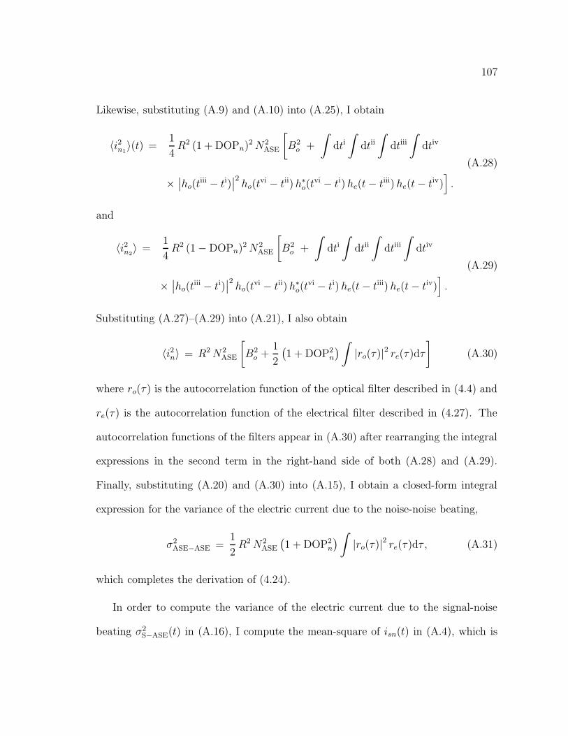
107
Likewise, substituting (A.9) and (A.10) into (A.25), I obtain
〈i2n1〉(t) =
1
4R2 (1 + DOPn)2N2
ASE
[
B2o +
∫
dti∫
dtii∫
dtiii∫
dtiv
×∣
∣ho(tiii − ti)
∣
∣
2ho(t
vi − tii) h∗o(tvi − ti) he(t− tiii) he(t− tiv)
]
.
(A.28)
and
〈i2n2〉 =
1
4R2 (1 − DOPn)2N2
ASE
[
B2o +
∫
dti∫
dtii∫
dtiii∫
dtiv
×∣
∣ho(tiii − ti)
∣
∣
2ho(t
vi − tii) h∗o(tvi − ti) he(t− tiii) he(t− tiv)
]
.
(A.29)
Substituting (A.27)–(A.29) into (A.21), I also obtain
〈i2n〉 = R2N2ASE
[
B2o +
1
2
(
1 + DOP2n
)
∫
|ro(τ)|2 re(τ)dτ
]
(A.30)
where ro(τ) is the autocorrelation function of the optical filter described in (4.4) and
re(τ) is the autocorrelation function of the electrical filter described in (4.27). The
autocorrelation functions of the filters appear in (A.30) after rearranging the integral
expressions in the second term in the right-hand side of both (A.28) and (A.29).
Finally, substituting (A.20) and (A.30) into (A.15), I obtain a closed-form integral
expression for the variance of the electric current due to the noise-noise beating,
σ2ASE−ASE =
1
2R2N2
ASE
(
1 + DOP2n
)
∫
|ro(τ)|2 re(τ)dτ , (A.31)
which completes the derivation of (4.24).
In order to compute the variance of the electric current due to the signal-noise
beating σ2S−ASE(t) in (A.16), I compute the mean-square of isn(t) in (A.4), which is

108
equal to
〈i2sn(t)〉 = R2⟨[
eso,1(t) e∗no,1
(t) ∗ he(t)] [
e∗so,1(t) eno,1
(t) ∗ he(t)]⟩
+R2⟨[
eso,2(t) e∗no,2
(t) ∗ he(t)] [
e∗so,2(t) eno,2
(t) ∗ he(t)]⟩
.
(A.32)
Substituting (A.9), (A.10), and (A.17) into (A.32), I obtain
σ2S−ASE(t) = 〈i2sn(t)〉 = R2 (1 + DOPn)NASE
×∫
dti∫
dtiies1,o(ti) e∗s1,o
(tii) ro(ti − tii) he(t− ti) he(t− tii)
+R2 (1 − DOPn)NASE
×∫
dti∫
dtiies2,o(ti) e∗s2,o
(tii) ro(ti − tii) he(t− ti) he(t− tii),
(A.33)
which is the variance of the electric current due to the signal-noise beating for an
arbitrarily polarized signal and an arbitrarily polarized noise. The integral expressions
in (A.33) can be rearranged so that
σ2S−ASE(t) = R2 (1 + DOPn)NASE
×∫
es1,o(τ)he(t− τ)
∫
e∗s1,o(τ ′)he(t− τ ′)ro(τ − τ ′)dτ ′dτ
+R2 (1 − DOPn)NASE
×∫
es2,o(τ)he(t− τ)
∫
e∗s2,o(τ ′)he(t− τ ′)ro(τ − τ ′)dτ ′dτ.
(A.34)
If one assumes that the signal is polarized, then the unit Jones vector that de-
fines the polarization state of the signal es is time-independent, so that es1,o(t) =

109
(es · a1) eso(t) and es2,o
(t) = (es · a2) eso(t) are the optically filtered parts of the noise-
free signal decomposed in the a1 and a2 orthogonal polarization states. Using these
results, I can rearrange (A.34) as
σ2S−ASE(t) = R2NASE
[
(1 + DOPn) |es · a1|2 + (1 − DOPn) |es · a2|2]
×∫
eso(τ)he(t− τ)
∫
e∗so(τ ′)he(t− τ ′)ro(τ − τ ′)dτ ′dτ,
(A.35)
which completes the derivation of (4.28).

Bibliography
[1] R. Newman, “Exitation of the Nd3+ fluorescence in CaWO4 by recombination
radiation in GaAs,” J. Appl.Phys., vol. 34, pp. 437–438, 1963.
[2] R. J. Keyes and T. M. Quist, “Injection luminescent pumping of CaF2:U2+ with
GaAs diode lasers,” Appl. Phys. Lett., vol. 4, pp. 50–52, 1964.
[3] F. P. Kapron, D. B. Keck, and R. D. Maurer, “Radiation losses in glass optical
waveguides,” Appl. Phys. Lett., vol. 17, pp. 423–425, 1970.
[4] R. J. Mears, L. Reekie, I. M. Jauneey, and D. N. Payne, “Low-noise erbium-doped
fibre amplifier operating at 1.45 µm,” Electron. Lett., vol. 23, pp. 1026–1028,
1987.
[5] I. P. Kaminow and I. L. Koch, Optical Fiber Telecommunications, vol. III-A,
San Diego, CA: Academic, 1997.
[6] H. Bulow, W. Baumert, H. Schmuck, F. Mohr, T. Schulz, F. Kuppers, and
W. Weiershausen, “Measurement of the maximum speed of PMD fluctuation in
installed field fiber,” in Proceedings OFC 1999, paper WE4, 1999.
110

111
[7] E. Lichtman, “Limitations imposed by polarization-dependent gain and loss on
all-optical ultralong communication systems,” J. Lightwave Technol., vol. 13,
pp. 906–913, 1995.
[8] D. Wang and C. R. Menyuk, “Calculation of penalties due to polarization effects
in a long-haul WDM system using a Stokes parameter model,” J. Lightwave
Technol., vol. 19, pp. 487–494, 2001.
[9] C. D. Poole and R. E. Wagner, “Phenomenological approach to polarization
dispersion in long single-mode fibers,” Electron. Lett., vol. 22, pp. 1029–1030,
1986.
[10] I. P. Kaminow and I. L. Koch, Optical Fiber Telecommunications, vol. III-B,
San Diego, CA: Academic, 1997.
[11] C. R. Menyuk and P. K. A. Wai, “Polarization evolution and dispersion in fibers
with spatially varying birefringence,” J. Opt. Soc. Am. B, vol. 11, pp. 1288–1296,
1994.
[12] C. D. Poole, R. W. Tkach, A. R. Chraplyvy, and D. A. Fishman, “Fading in
lightwave systems due to polarization-mode dispersion,” IEEE Photon. Technol.
Lett., vol. 3, pp. 68–70, 1991.
[13] R.-M. Mu, V. S. Grigoryan, C. R. Menyuk, G. M. Carter, and J. M. Jacob,
“Comparison of theory and experiment for dispersion-managed solitons in a re-
circulating fiber loop,” IEEE J. of Selected Topics in Quantum Electron., vol. 6,
pp. 248–257, 2000.

112
[14] M. G. Taylor, “Improvement in Q with low frequency polarization modulation
on transoceanic EDFA link,” IEEE Photon. Technol. Lett., vol. 6, pp. 860–862,
1994.
[15] N. S. Bergano, F. W. Kerfoot, and C. R. Davidson, “Margin measurements in
optical amplifier systems,” IEEE Photon. Technol. Lett., vol. 5, pp. 304–306,
1993.
[16] I. T. Lima Jr., A. O. Lima, J. Zweck, and C. R. Menyuk, “Efficient computation
of outage probabilities due to polarization effects in a WDM system using a
reduced Stokes model and importance sampling,” IEEE Photon. Technol. Lett.,
vol. 15, pp. 45–47, 2003.
[17] P. M. Hahn and M. C. Jeruchim, “Developments in the theory and application
of importance sampling,” IEEE Trans. Commun., vol. 35, pp. 706–714, 1987.
[18] D. Marcuse, “Derivation of analytical expressions for the bit-error probability
in lightwave systems with optical amplifiers,” J. Lightwave Technol., vol. 8, pp.
1816–1823, 1990.
[19] P. A. Humblet and M. Azizoglu, “On the bit error rate of lightwave systems
with optical amplifiers,” J. Lightwave Technol., vol. 9, pp. 1576–1582, 1991.
[20] P. J. Winzer, M. Pfennigbauer, M. M. Strasser, and W. R. Leeb, “Optimum filter
bandwidth for optically preamplified NRZ receivers,” J. Lightwave Technol., vol.
19, pp. 1263–1273, 2001.

113
[21] Y. Sun, I. T. Lima Jr., A. O. Lima, H. Jiao, L. Yan, J. Zweck, C. R. Menyuk, and
G. M. Carter, “Effects of partially polarized noise in a receiver,” in Proceedings
OFC 2003, paper MF82, 2003.
[22] Y. Sun, A. O. Lima, I. T. Lima Jr., L. Yan, J. Zweck, C. R. Menyuk, and G. M.
Carter, “Accurate Q-factor distributions in optical transmission systems with
polarization effects,” in Proceedings OFC 2003, paper ThJ4, 2003.
[23] H. Jiao, I. T. Lima Jr., A. O. Lima, Y. Sun, J. Zweck, L. Yan, C. R. Menyuk, and
G. M. Carter, “Experimental validation of an accurate receiver model for systems
with unpolarized noise,” in Proceedings CLEO 2003, paper CThJ1, 2003.
[24] B. E. A. Saleh and M. C. Teich, Fundamentals of Photonics, New York: John
Wiley & Sons, 1991.
[25] M. Born and E. Wolf, Principles of Optics, Cambridge, UK: Cambridge Univer-
sity Press, 1999.
[26] J. D. Jackson, Classical Electrodynamics, New York, NY: John Wiley & Sons,
1999.
[27] D. Marcuse, C. R. Menyuk, and P. K. A. Wai, “Application of the Manakov-
PMD equation to studies of signal propagation in optical fibers with randomly
varying birefringence,” J. Lightwave Technol., vol. 15, pp. 1735–1746, 1997.
[28] I. P. Kaminow, “Polarization in optical fibers,” IEEE J. Quantum Electron.,
vol. 17, pp. 15–22, 1981.

114
[29] C. R. Menyuk, “Application of multiple-length-scale methods to the study of
optical fiber transmission,” J. Eng. Math., vol. 36, pp. 113–136, 1999.
[30] E. Golovchenko, “The challenges of designing long-haul WDM systems,” in
Tutorial Sessions OFC 2002, paper TuL, 2002.
[31] E. A. Golovchenko, A. N. Pilipetskii, N. S. Bergano, C. R. Davidson, F. I. Khatri,
R. M. Kimball, and V. J. Mazurczyk, “Modeling transoceanic fiber-optic WDM
communication systems,” IEEE J. Select. Topics Quantum Electron., vol. 6, pp.
224–226, 2000.
[32] G. Poole and D. L. Favin, “Polarization dispersion measurements based on
transmission spectra through a polarizer,” J. Lightwave Technol., vol. 12, pp.
917–929, 1994.
[33] G. Biondini, W. L. Kath, and C. R. Menyuk, “Importance sampling for
polarization-mode dispersion,” IEEE Photon. Technol. Lett., vol. 14, pp. 310–
312, 2002.
[34] G. P. Agrawal, Nonlinear Fiber Optics, San Diego: Academic Press, 1995.
[35] H. Goldstein, Classical Mechanics, Reading, MA: Addison-Wesley, 1980.
[36] F. Corsi, A. Galtarossa, and L. Palmieri, “Polarization mode dispersion charac-
terization of single-mode optical fiber using backscattering technique,” J. Light-
wave Technol., vol. 16, pp. 1832–1843, 1998.
[37] D. Wang, Polarization effects in dense WDM systems, Ph.D. Dissertation,
University of Maryland Baltimore County, Baltimore, MD, May 2000.

115
[38] G. P. Agrawal, Fiber Optic Communication Systems, New York: Wiley-
Interscience, 1997.
[39] L. Kazovsky, S. Benedetto, and A. Willner, Optical Fiber Communication Sys-
tems, Norwood, MA: Artech House, 1996.
[40] C. R. Menyuk, B. S. Marks, I. T. Lima Jr., J. Zweck, Y. Sun, G. M. Carter, and
D. Wang, “Polarization effects in long-haul undersea systems,” Undersea Fibre
Communication Systems, Jose Chesnoy, ed., San Diego, CA: Academic Press,
2002, Sec. II.D.
[41] G. Arfken, Mathematical Methods for Physicists, San Diego, CA: Academic
Press, 1985.
[42] A. Carena, V. Curri, R. Gaudino, P. Poggiolini, and S. Benedetto, “A time-
domain optical transmission system simulation package accounting for nonlinear
and polarization-related effects in fiber,” J. Sel. Areas Commun., vol. 15, pp.
751–765, 1997.
[43] R. Holzlohner, C. R. Menyuk, V. S. Grigoryan, and W. L. Kath, “Accurate
calculation of eye diagrams and error rates in long-haul transmission systems
using linearization,” J. Lightwave Technol., vol. 20, pp. 389–400, 2002.
[44] I. P. Kaminow and I. L. Koch, Optical Fiber Telecommunications, vol. III-B,
San Diego, CA: Academic, 1997.

116
[45] I. T. Lima Jr., A. O. Lima, J. Zweck, and C. R. Menyuk, “Performance charac-
terization of chirped return-to-zero modulation format using an accurate receiver
model,” IEEE Photon. Technol. Lett., vol. 15, pp. 608–610, 2003.
[46] R. Holzlohner, C. R. Menyuk, W. L. Kath, and V. S. Grigoryan, “Efficient and
accurate calculation of eye diagrams and bit-error rates in a single-channel CRZ
system,” IEEE Photon. Technol. Lett., vol. 14, pp. 1079–1081, 2002.
[47] E. Desurvire, Erbium Doped Fiber Amplifiers, New York, NY: John Wiley &
Sons, 1994.
[48] P. R. Trischitta and E. L. Varma, Jitter in Digital Transmission Systems, Boston:
Artech House, 1989.
[49] R. E. Walpole and R. H. Myers, Probability and Statistics for Engineers and
Scientists, New York, NY: Macmillan Publishing Co., 1993.
[50] R.-M. Mu., T. Yu, V. S. Grigoryan, and C. R. Menyuk, “Dynamics of the chirped
return-to-zero modulation format,” J. Lightwave Technol., vol. 20, pp. 47–57,
2002.
[51] R. Y. Rubinstein, Simulation and the Monte Carlo Method, New York: John
Wiley & Sons, 1981.
[52] M. C. Jeruchim, P. Balaban, and K. S. Shanmugan, Simulation of Communi-
cation Systems: Modeling, Methodology, and Techniques: Plenum Publishing
Corp., 2001.

117
[53] R. P. Brent, Algorithms for Minimization without Derivatives, Englewood Cliffs,
NJ: Pretice Hall, 1973.
[54] E. Veach, Robust Monte Carlo methods for light transport simulation, Ph.D.
Dissertation, Stanford University, Palo Alto, CA, December 1997.
[55] I. T. Lima Jr., A. O. Lima, G. Biondini, C. R. Menyuk, and W. L. Kath, “A
comparative study of single-section polarization-mode dispersion compensators,”
J. Lightwave Technol., Special Issue—PMD, to appear in May 2003.
[56] L.-S. Yan, Q. Yu, Y. Xie, and A. E. Willner, “Experimental demonstration of
the system performance degradation due to the combined effects of polarization-
dependent loss with polarization-mode dispersion,” IEEE Photon. Technol. Lett.,
vol. 14, pp. 224–226, 2002.
[57] Y. Sun, I. T. Lima Jr., H. Jiao, J. Wen, H. Xu, H. Ereifej, G. Carter, and
C. R. Menyuk, “Study of system performance in a 107 km dispersion-managed
recirculating loop due to polarization effects,” IEEE Photon. Technol. Lett., vol.
13, pp. 966–968, 2001.
[58] P. K. A. Wai, C. R. Menyuk, and H. H. Chen, “Stability of solitons in randomly
varying birefringent fibers,” Optics Lett., vol. 16, pp. 1231–1233, 1991.