visualization with paraview - hpc...
TRANSCRIPT

Visualization with ParaView
Arizona State University 2014
Before we begin… • Make sure you have ParaView 4.1.0 installed so you
can follow along in the lab section – http://paraview.org/paraview/resources/software.php

Background • http://www.paraview.org/ • Open-source, multi-platform parallel data analysis
and visualization application • Mature, feature-rich interface • Good for general-purpose, rapid visualization • Built upon the Visualization ToolKit (VTK) library • Primary contributors:
– Kitware, Inc. – Sandia National Laboratory – Los Alamos National Laboratory – Army Research Laboratory

Data Types • Supports a wide variety of data types
– Structured grids • uniform rectilinear, non-uniform rectilinear, and
curvilinear – Unstructured grids – Polygonal data – Images – Multi-block – AMR
• Time series support
*http://www.paraview.org/Wiki/images/c/c6/ParaViewTutorial312.pdf
*

Visualization Algorithms • Supports a wide variety of visualization
algorithms -> Filters – Isosurfaces – Cutting planes – Streamlines – Glyphs – Volume rendering – Clipping – Height maps – …

Special Features
• Supports derived variables – New scalar / vector variables that are
functions of existing variables in your data set • Scriptable via Python • Saves animations • Can run in parallel / distributed mode for
large data visualization

Data Formats • Supports a wide variety of data formats
– VTK (http://www.vtk.org/VTK/img/file-formats.pdf) – EnSight – Plot3D – Various polygonal formats
• Users can write data readers to extend support to other formats
• Conversion to the VTK format is straightforward

Data Formats
• VTK Simple Legacy Format • ASCII or binary • Supports all VTK grid
types • Easiest for data
conversion
• Note: use VTK XML format for parallel I/O
VTK simple legacy format (http://www.vtk.org/VTK/img/file-formats.pdf)

Data Formatting Example • Data set: 4x4x4 rectilinear grid
with one scalar variable

ParaView Visualization Pipeline
• All processing operations (filters) produce data sets
• Can further process the result of every operation to build complex visualizations – e.g. can extract a cutting plane, and apply
glyphs (i.e. vector arrows) to the result • Gives a plane of glyphs through your 3D volume
Demonstration • WRF weather forecast data set
– Rectilinear grid – Multiple scalar and vector variables – Time series
• Can show:
– Clouds – Wind – Temperature – …


ParaView Test-Drive

Getting Started
• Download example data file • ‘disk_out_ref.ex2’
– http://portal.longhorn.tacc.utexas.edu/training/ – Right-click, Save link as…
• Open ParaView

ParaView Menu Bar
Toolbars
Pipeline Browser
Object Inspector
3D View
(well, this is a Mac)
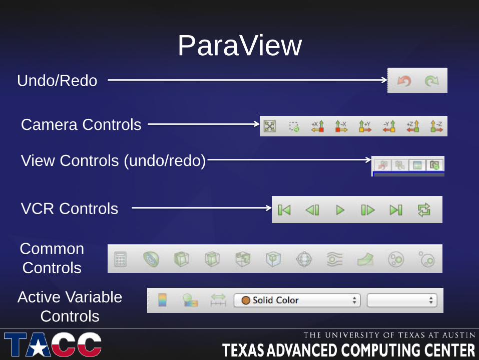
ParaView Undo/Redo
Camera Controls
View Controls (undo/redo)
VCR Controls
Common Controls
Active Variable Controls

ParaView Today we will: • Create isosurfaces for a scalar
variable • Clip and slice the surfaces • Use glyphs to display a vector
field • Use streamlines to show flow
through a vector field • Edit color maps • Add slices to show variable
values over a plane • Add color legends • Create volume rendering • Create a plot over a line

ParaView
Open the file disk_out_ref.ex2
• Click File -> Open • Select
disk_out_ref.ex2 • Click OK • Select ALL variables • Click blue Apply • Cylinder outline of
dataset extent displayed

ParaView
Open the file disk_out_ref.ex2
• Click File -> Open • Select
disk_out_ref.ex2 and click OK

ParaView
Open the file disk_out_ref.ex2
• Click File -> Open • Select
disk_out_ref.ex2 and click OK
• Select ALL variables

ParaView
Open the file disk_out_ref.ex2
• Click File -> Open • Select
disk_out_ref.ex2 • Click OK • Select ALL variables • Click blue Apply

ParaView
Open the file disk_out_ref.ex2
• Click File -> Open • Select
disk_out_ref.ex2 • Click OK • Select ALL variables • Click blue Apply
Cylinder outline of
dataset extent displayed

ParaView Manipulate Representation and color • Use the Active Variable
Controls to change color Solid Color -> Pres

ParaView Manipulate Representation and color • Use the Active Variable
Controls to change color Solid Color -> Pres

ParaView Manipulate Representation and color • Use the Active Variable
Controls to change color Solid Color -> Pres
• Use Representation toolbar to change representation
Surface -> Surface With Edges

ParaView Manipulate Representation and color • Use the Active Variable
Controls to change color Solid Color -> Pres
• Use Representation toolbar to change representation
Surface -> Surface With Edges
ParaView Manipulate Representation and color • Use the Active Variable
Controls to change color Solid Color -> Pres
• Use Representation toolbar to change representation
Surface -> Surface With Edges
• Show Colorbar annotation

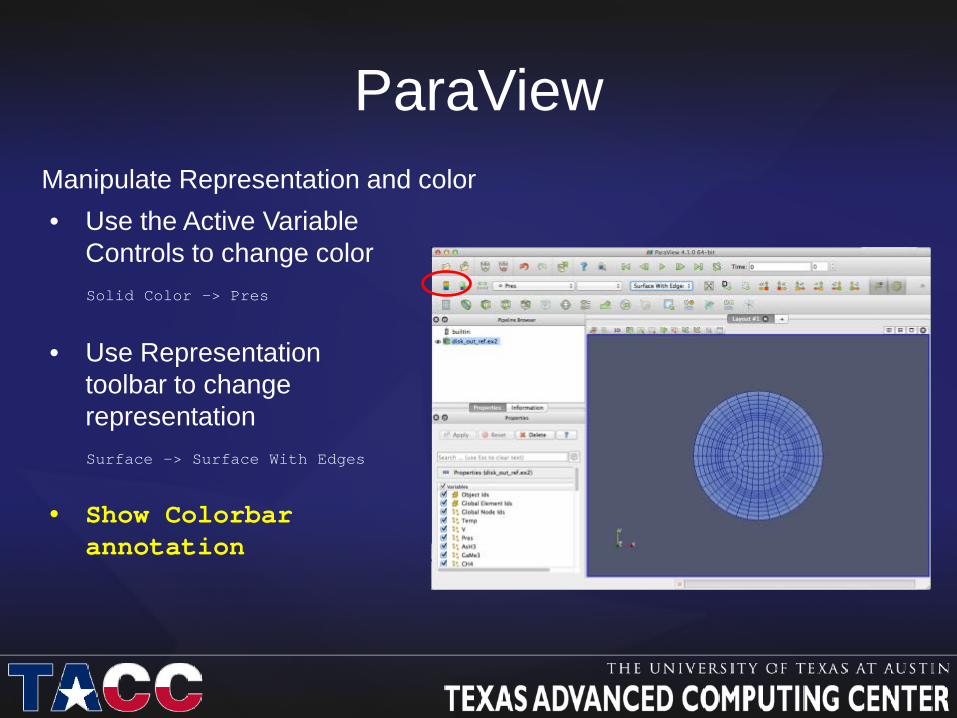
ParaView Manipulate Representation and color • Use the Active Variable
Controls to change color Solid Color -> Pres
• Use Representation toolbar to change representation
Surface -> Surface With Edges
• Show Colorbar annotation

• Explore dataset with mouse
ParaView
• Click +Z view button

• Explore dataset with mouse
ParaView
• Click +Z view button • Huh?

• Explore dataset with mouse
ParaView
• Click +Z view button • Huh?
• Move it around

• Explore dataset with mouse
ParaView
• Click +Z view button • Huh?
• Move it around
• Change Representation

ParaView
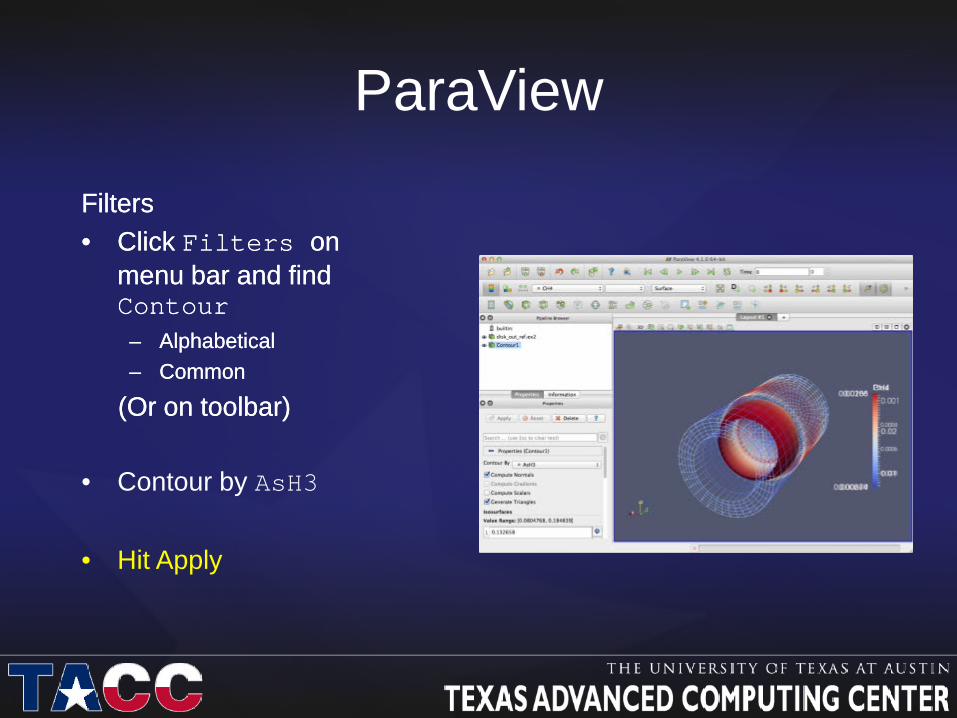
Filters • Click Filters on
menu bar and find Contour
– Alphabetical – Common
(Or on toolbar)

ParaView
Filters • Click Filters on
menu bar and find Contour
– Alphabetical – Common
(Or on toolbar)
• Contour by AsH3
ParaView
Filters • Click Filters on
menu bar and find Contour
– Alphabetical – Common
(Or on toolbar)
Filters • Click Filters on
menu bar and find Contour
– Alphabetical – Common
(Or on toolbar)
• Contour by AsH3
• Hit Apply

ParaView
Filters • With Contour1
selected, use Active Variable Control to color by CH4
• And drag one of the colorbars elsewhere

ParaView
Filters • With Contour1
selected, use Active Variable Control to color by CH4
• And drag one of the colorbars elsewhere

ParaView
Filters (2) • Click Filters on
menu bar and find Clip
– Alphabetical – Common
(Or on toolbar)

ParaView
Filters (2) • Choose orientation
axes

ParaView
Filters (2) • Hit Apply
• Note: all three
objects are visible – Wireframe of
dataset – Contour surface – Surface of clipped
dataset
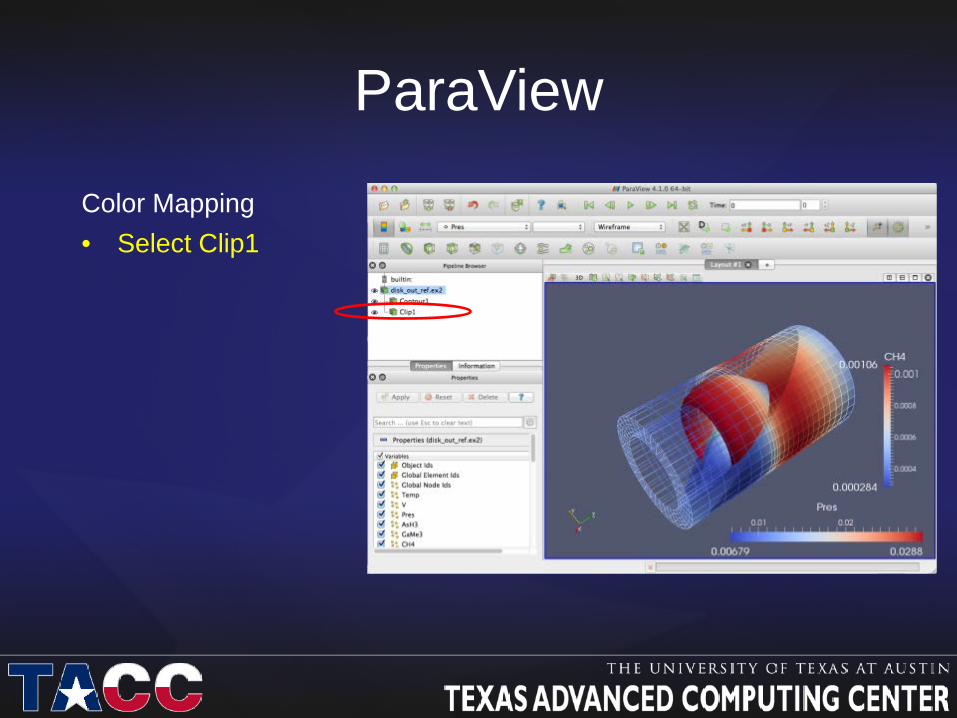
ParaView
Color Mapping • Select Clip1

ParaView
Color Mapping • Select Edit Color Map

ParaView
Color Mapping • Select Edit Color Map

ParaView
Color Mapping • Select Choose Preset
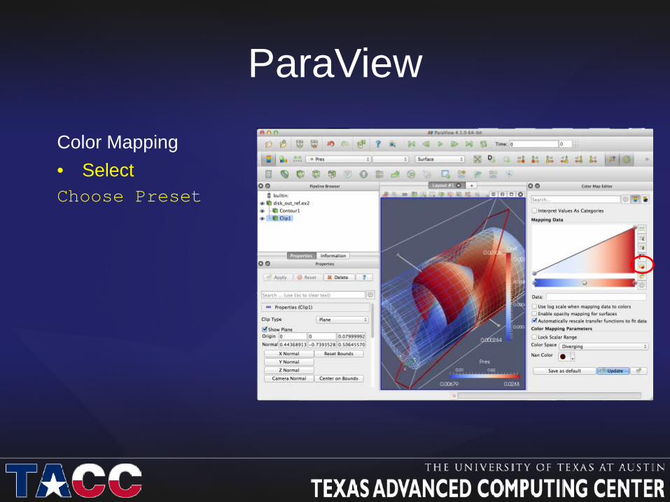
ParaView
Color Mapping • Select Choose Preset
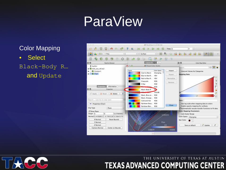
ParaView
Color Mapping • Select Black-Body R…
and Update

ParaView
Color Mapping • Select Black-Body R…
and Close
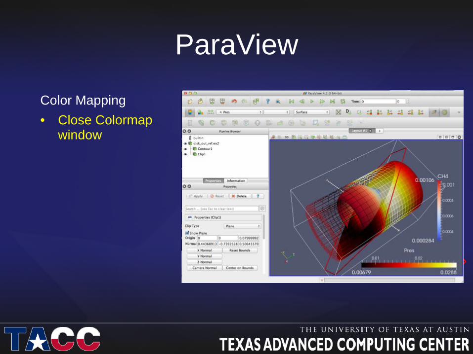
ParaView
Color Mapping • Close Colormap
window

ParaView
Filters (3) • Select original
dataset
• Click Filters on menu bar and find Stream Tracer
– Alphabetical – Common
(Or on toolbar)

ParaView
Filters (3) • Scroll down on
Properties pane until you see seeds sub-pane
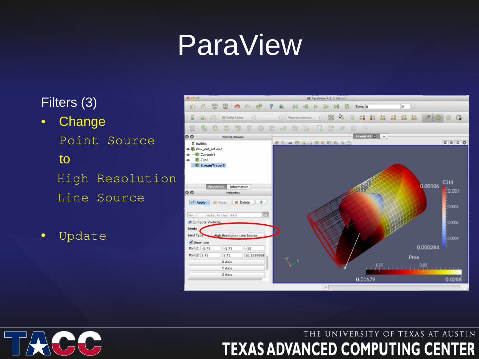
ParaView
Filters (3) • Change Point Source to High Resolution
Line Source
• Update

ParaView
Filters (3) • You can manipulate
the ‘rake’ interactively
• You can change the number of seed points
• You can change the interpolation method yadda yadda

ParaView
Filters (3) • With
StreamTracer1 selected,
• Click Filters on menu bar and find Tube
– Alphabetical – ?
• Update

ParaView
Filters (3)

ParaView
Filters (3) • Turn on Wire Frame
of original dataset • Hide Tube’d
Stream lines
ParaView
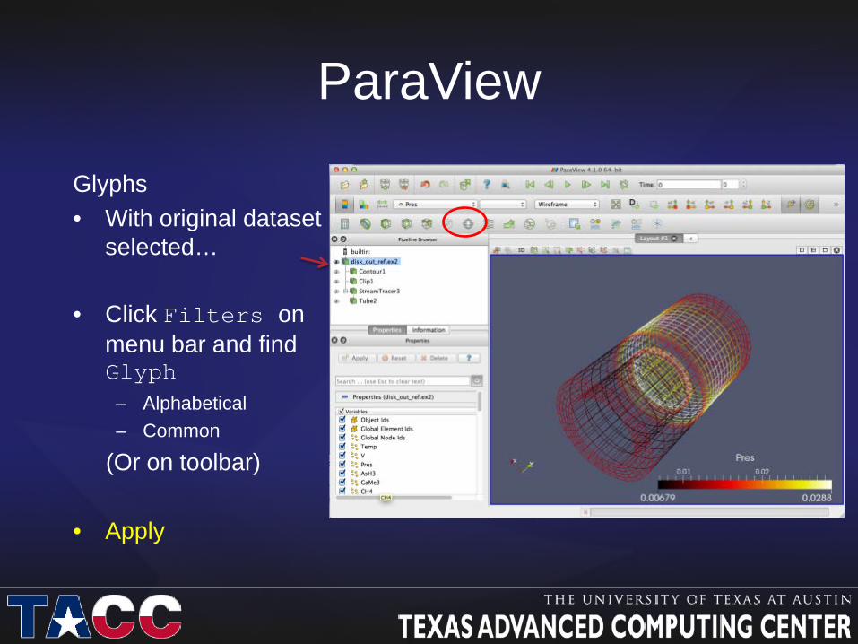
Glyphs • With original dataset
selected…
• Click Filters on menu bar and find Glyph
– Alphabetical – Common
(Or on toolbar) • Apply
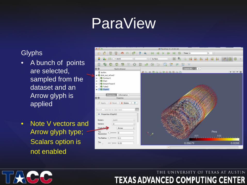
ParaView
Glyphs • A bunch of points
are selected, sampled from the dataset and an Arrow glyph is applied
• Note V vectors and Arrow glyph type;
Scalars option is not enabled

ParaView
Glyphs • Scroll down in
properties window and change Scale Mode to scalar
• Scroll back …
• Set Glyph Type to sphere
• Choose any variable and Apply
ParaView
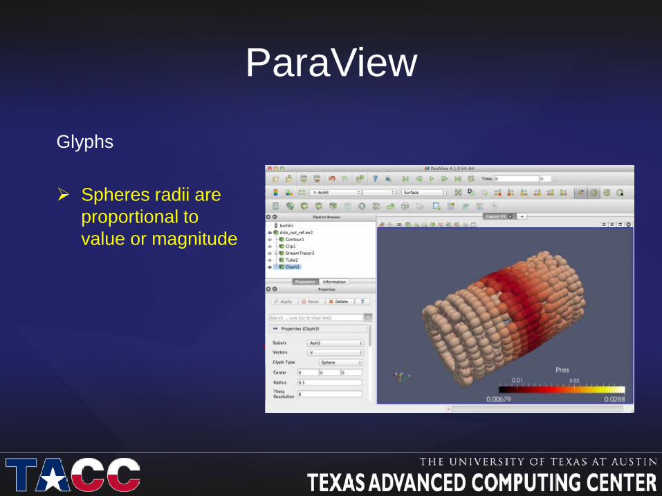
Glyphs Spheres radii are
proportional to value or magnitude

ParaView
Glyphs • With the Glyphs
selected…
• Edit->Change Input…

ParaView
Glyphs • Select the Stream
Trace, Apply

ParaView
Glyphs Note dependency
tree
• With the Glyph selected, change Scale Mode to Vector, Glyph Type to Arrow, and choose variable v
• Apply

ParaView
Glyphs Glyphs are now
tangential arrows

ParaView
Volume Rendering • Delete everything
except original dataset
• Set Representation to Volume
ParaView
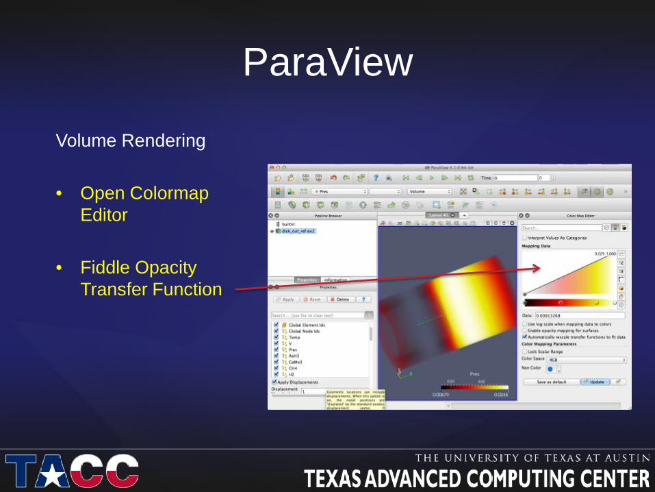
Volume Rendering • Open Colormap
Editor
• Fiddle Opacity Transfer Function

ParaView
Volume Rendering • … to look like this
• Close Colormap
Editor

ParaView
Volume Rendering
• And we can then
add a new contour, streamlines, yadda yadda

ParaView
Volume Rendering • Notice smallwrf
directory
• Enter it

ParaView
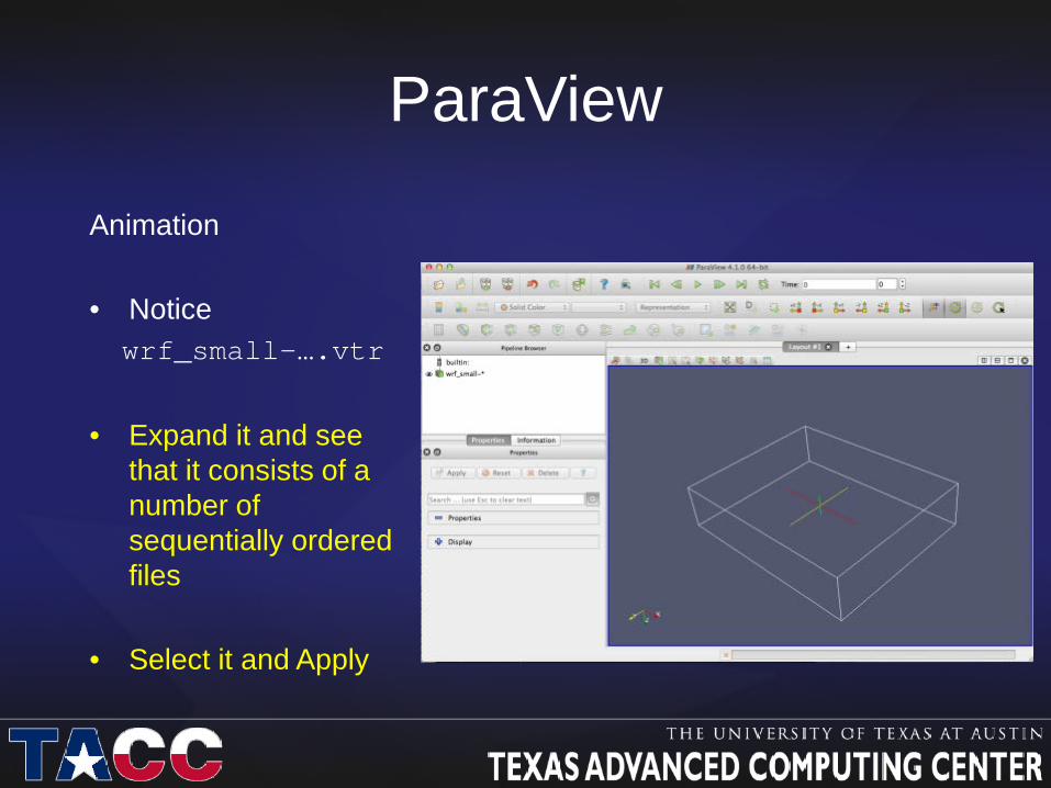
Animation • Notice wrf_small-….vtr • Expand it and see
that it consists of a number of sequentially ordered files
• Select it and Apply
ParaView
Animation • Notice wrf_small-….vtr • Expand it and see
that it consists of a number of sequentially ordered files
• Select it and Apply

ParaView
Animation • Select Contour
• Contour By: QRAIN
• Set Value Range 0.0001 • Apply
• Hit Play

ParaView
Saving Animation • File->Save Animation…
• Set output resolution • Hit Save Animation

ParaView
Saving Animation • Create Directory
• e.g. movie1
• Enter that directory

ParaView
Saving Animation • Set File Name
• e.g. ‘frame’
• Set Files to Type
• I use ‘avi’
• OK

Questions?
• More tutorials available: – http://www.paraview.org/Wiki/The_ParaView_Tutorial