vision-based guidance system for a 6-dof robot
TRANSCRIPT

VISION-BASED GUIDANCE SYSTEM FOR A 6-DOF
ROBOT
Bachelor’s thesis
Automation Engineering
Valkeakoski, spring, 2014
Ignacio Torroba Balmori

BACHELOR’S THESIS
Title Visual-based Guidance System for a 6-DOF Robot
Author Ignacio Torroba Balmori
Supervised by Raine Lehto
Approved on _____._____.20_____
Approved by

1
ABSTRACT
Valkeakoski
Bachelor in Automation Engineering
Author Ignacio Torroba Balmori Year 2014
Subject of Bachelor’s thesis Visual-based Guidance System for a 6-DOF Robot
ABSTRACT
The idea of this bachelor’s thesis is to develop a position-based visual servoing system with
two webcams that allows an anthropomorphic robot ABB IRB 120 with six degrees of
freedom (DOF) to be guided in real time by an operator, by triangulating a specific target
moved within the field of view (FOV) of a machine vision system. For this kind of motion
control based on visual data input, termed visual servoing control, we need a stereo vision
system to acquire the images of the target since three-dimensional information is required
to perform object tracking with six DOF. These images are processed by a MATLAB ap-
plication running in a remote PC. The current coordinates of the target referred to the left
camera reference frame are extracted from the images and sent through an Ethernet connec-
tion to the robot controller, which is programmed to receive the vectors and move its tool
centre point (TCP) to the demanded position within its workspace.
The image acquisition and processing algorithm have been developed entirely in MATLAB
instead of in other programming languages (such as C/C++), mainly because of the large
amount of available toolboxes and MATLAB's elegant vector/matrix operations. These
MATLAB’s features have greatly reduced the time involved from the idea to the final code.
The communication link between the PC and the IRC5 controller has been implemented via
a NFS server-client and the use of binary semaphores for the multi-process synchronization
in the implemented producer-consumer structure. And RobotStudio has been used to pro-
gram the RAPID application and to create the new reference frame for the robot system,
since the robot is an ABB model and has its own high-level programming language.
As a result of the project, the robot’s end-effector can be guided by the user, who controls
its current location by moving the target in the overlapped FOV of the cameras, which
models the robot workspace. This is a simple and intuitive method for the operator of the
robot to perform specific 3D movements with its tool in real-time.
Keywords Camera calibration, stereo triangulation, Network File System, RAPID lan-
guage.
Pages 78 pp. + appendices 2 pp.

2
ACKNOWLEDGMENTS
This Bachelor’s thesis, with all the previous years of learning and work that have led me to
finish it today, is dedicated to all those who let me make it possible, since the very
beginning.

3
CONTENTS
ABSTRACT ...................................................................................................................... I
ACKNOWLEDGMENTS ................................................................................................ II
1 INTRODUCTION ....................................................................................................... 6
1.1 OBJETIVES OF THE PROJECT ....................................................................... 6
1.2 STRUCTURE OF THE PROJECT ..................................................................... 7
2 MACHINE VISION SYSTEM ................................................................................... 8
2.1 INTRODUCTION ............................................................................................... 8
2.2 CAMERA MODEL ............................................................................................ 8
2.2.1 Perspective projective .............................................................................. 8
2.2.2 Projection through the camera pinhole model ......................................... 9
2.2.3 Defining the model of the camera ......................................................... 10
2.2.4 Matrix of complete projection ............................................................... 13
2.2.5 Lens distortion ....................................................................................... 14
2.3 CALIBRATION PROCESS ............................................................................. 16
2.3.1 Introduction ........................................................................................... 16
2.3.2 Calibration methods ............................................................................... 16
2.3.3 Obtaining the projection matrix ............................................................. 17
2.4 CAMERA CALIBRATION WITH MATLAB TOOLBOX ............................ 20
2.4.1 Patterns for calibration .......................................................................... 20
2.4.2 Calibration with planar pattern .............................................................. 21
2.4.3 Camera calibration toolbox in MATLAB ............................................. 22
2.5 BINOCULAR VISION ..................................................................................... 23
2.6 STEREO VISION ............................................................................................. 24
2.6.1 One camera systems .............................................................................. 24
2.6.2 Two cameras systems ............................................................................ 25
2.6.3 Triangulation ......................................................................................... 25
2.7 PARAMETERS OF THE STEREOVISION SYSTEM ................................... 30
2.7.1 The Logitech HD Webcam C270 .......................................................... 30
2.7.2 The location of the cameras ................................................................... 32
2.7.3 Illumination ........................................................................................... 35
2.7.4 Structure of the system .......................................................................... 36
2.8 ALGORITHM DEVELOPMENT .................................................................... 38
2.8.1 Introduction ........................................................................................... 38
2.8.2 Steps in the development ....................................................................... 39
2.8.3 Diagram of the algorithm ...................................................................... 48

4
3 COMMUNICATION INTERFACE ......................................................................... 50
3.1 INTRODUCTION ............................................................................................. 50
3.2 APPROACH TO THE PROBLEM .................................................................. 50
3.3 PARALLEL COMPUTING .............................................................................. 50
3.3.1 Producer-Consumer problem ................................................................. 51
3.4 PROCESSES SYNCHRONIZATION .............................................................. 51
3.4.1 Flow control problems ........................................................................... 51
3.4.2 Mutual exclusion ................................................................................... 53
3.5 REAL IMPLEMENTATION ............................................................................ 55
3.5.1 The IRC5 Compact controller ............................................................... 55
3.5.2 The remote PC ....................................................................................... 57
3.6 SOFTWARE ..................................................................................................... 57
3.6.1 Network communications ...................................................................... 57
3.6.2 The Network File Sytem ....................................................................... 59
3.7 FINAL IMPLEMENTATION .......................................................................... 59
3.7.1 The NFS server ...................................................................................... 59
3.7.2 The NFS client ....................................................................................... 60
3.7.3 Semaphores in NFS ............................................................................... 62
3.7.4 Common buffer in NFS ......................................................................... 62
3.7.5 Data frame ............................................................................................. 62
4 PROGRAMMING THE ROBOT ............................................................................. 63
4.1 INTRODUCTION ............................................................................................. 63
4.2 MANIPULATING ROBOTS ........................................................................... 63
4.2.1 Industrial robot definition ...................................................................... 63
4.2.2 Morphology of the robot ....................................................................... 64
4.3 ABB IRB 120 .................................................................................................... 67
4.3.1 Description ............................................................................................ 67
4.3.2 Technical specifications ........................................................................ 67
4.4 IRC 5 COMPACT CONTROLLER ................................................................. 68
4.5 PATH GENERATION IN ROBOTICS ............................................................ 69
4.5.1 Kinematic control .................................................................................. 69
4.5.2 Kinematic control inputs ....................................................................... 70
4.6 ROBOTSTUDIO AND RAPID LANGUAGE ................................................. 71
4.6.1 RobotStudio ........................................................................................... 71
4.6.2 RAPID language .................................................................................... 71
4.7 RAPID PROGRAM .......................................................................................... 72
4.7.1 Critical section ....................................................................................... 72
4.7.2 Non-critical section ............................................................................... 73
4.7.3 Diagram of the program ........................................................................ 75
5 CONCLUSIONS ....................................................................................................... 76
SOURCES ...................................................................................................................... 77

5
Appendix A IMAGE PROCESSING ALGORITHM IN MATLAB
Appendix B RAPID PROGRAM FOR THE ABB IRB 120

6
1 INTRODUCTION
1.1 OBJETIVES OF THE PROJECT
The main objective of this project is the design and implementation of a navi-
gation system for six DOF robots that lets the user to perform both the posi-
tion and the speed of the robot tool centre point (TCP) in a simple and com-
fortable way, so no previous experience is needed to operate the robot and a
secure distance can be kept between it and the rest of the system. The com-
plete system is shown in Figure 1 and each component is described in the fol-
lowing sections.
This system can be adapted to any other model of anthropomorphic robot
since the only parameters that need to be modified are the height of the cam-
eras (their field of view for the robot workspace) so the workspace and the de-
tection of singularities in the trajectories can be adjusted to the new model.
Vision Guided Robots (VGR) have been widely implemented in various in-
dustries. Mostly in the manufacturing environment where conditions can be
controlled and object position is deterministic. When the object is stationary,
its pose can be easily determined and robotic picking can be readily executed.
However, for specific tasks in which the control must be taken by an operator,
programming the motion is not an option so the robot must be always led by a
human, which represents more challenges. For this kind of situations, the de-
signed system can be an interesting option.
Figure 1.1 Vision guided robot system

7
1.2 STRUCTURE OF THE PROJECT
In order to carry out the whole project, it has been divided in three different
parts, which can be read in chapters 2, 3 and 4 of this report. The conclusions
and results can be found in chapter 5.
Chapter 2: The design and construction of the machine vision system
The stereovision system, consisting of two cameras fixed over an arc, takes
images of the target moved by the operator and tracks its position while it is
being moved within the overlapped FOV of the cameras. A PC running the
MATLAB programme processes the images and triangulates the position, and
if it belongs to the robot’s workspace, the vectors referred to the left camera’s
reference frame are stored to be sent.
Chapter 3: The search and implementation of the most suitable data transfer
method
A communication application via a Network File System is implemented to
enable the PC that processes the acquired images to share data with the robot
controller. Proceeding in this way, the vectors for the movement can be sent
through a common .txt file located in the hard disk of the computer, which
can be accessed by the robot as a local disk.
Chapter 4: Development of the RAPID program to be executed by the robot
The robot is programmed in RAPID language to read the vectors from the
common file and execute the necessary movements toward the desired
equivalent point in its own reference frame, which has been defined as a work
object in RobotStudio. Once these three parts have been reached separately,
several tests have been performed in order to assemble them and make the
whole system work properly.
Chapter 5: Conclusions and future works
The last chapter contains some conclusions about the whole thesis perfor-
mance as well as a discussion about the main ideas implemented and alterna-
tive ways to carry out the development with some other resources.

8
2 MACHINE VISION SYSTEM
2.1 INTRODUCTION
Throughout this chapter, the developed machine vision system is presented.
Starting with an introduction of the mathematical camera model used and the
process of image formation, the next points describe the steps taken during
the calibration of the stereo vision system and the challenges and solutions
presented in the design of the whole acquisition system. After this, the image
processing algorithm developed in MATLAB, which can be found in the ap-
pendix A, is explained.
2.2 CAMERA MODEL
A camera is a mapping between the 3D world (object space) and a 2D image,
which can be represented by matrices with particular properties, called cam-
era models. In the point, we are going to introduce the basis of this idea and
the camera model we have used throughout the project.
2.2.1 Perspective projective
As known, a dimension is lost when we project the real world on an image
through the image formation process using a camera. The complexity of this
process relies on the large quantity of elements that takes part on it. Among
them, the lens utilized has a special role.
In this project, the pinhole model (Figure 2) is going to be assumed for our
camera as far as it simplifies the analysis by disregarding the diffraction and
reflection effects of the lens. This means that we can apply the principle of
collinearity to the analysis, where each point in the object space is projected
by a straight line through the projection centre into the image plane (Hartley
& Zisserman, 2000).
Figure 2.1 Pinhole camera geometry

9
The perspective model of the camera, that maps the real 3D coordinates of the
object (X, Y, Z) on the image plane coordinates (x,y) is given by the equation
(2.1), ignoring the final image coordinate (z=f)
(2.1)
This is a non-linear relation given by the effective focal length of the camera,
where the negative sign in each equation means that the projected images are
inverted on the sensor plane (real screen). However, from now on we are go-
ing to use the virtual screen model (without signs) because it is more comfort-
able, with the coordinate system showed in Figure 2.2. In this system, the im-
age plane has been moved behind the optical centre but the z-axis of the cam-
era frame is still perpendicular to the image plane.
Figure 2.2 Coordinate system applied
2.2.2 Projection through the camera pinhole model
The mathematical model of the camera is used to express the relationship be-
tween a 3D point P=[X, Y, Z]T in normalized coordinates and its image pro-
jection p=[u, v]T in pixel coordinates, each ones in their reference frame, mak-
ing use of the pinhole model of the camera introduced before.
The equation of the projection is given as follows (Zhang, 1998)
(2.2)
Where s is an arbitrary scale factor, M is the matrix of the complete projec-
tion, which we need to obtain and T, T are the co-
ordinates’ vectors of the point in 2D and 3D in homogeneous coordinates.
The reason of the use of homogeneous coordinates will be explained below.

10
2.2.3 Defining the model of the camera
Some changes in the reference system both in the plane and in the space are
going to be necessary to establish a precise mapping between the 3D points
(P) referred to a fixed global reference frame and their projections in the im-
age (p), referred to an image’s local reference frame (Hartley & Zisserman,
2000). These are the three involved transformations:
2.2.3.1 Projection of the space coordinates to the plane coordinates
Once the virtual screen model of the pinhole model of the camera has been
chosen, the collinear relation between the real 2D coordinates of the object
and the image normalized coordinates, as said, is given by the conical projec-
tion equation (1.1). In order to project the space coordinates to the image co-
ordinates we need to solve the whole process of image formation and coordi-
nates transformation. This can be done by using dot matrices and homogene-
ous coordinates, so the equations of the conical projection become linear and
can be resolved easily.
So the equation of projection can be expressed compactly as follows:
(2.3)
2.2.3.2 Transformation of the reference frame in the image plane itself
Within the image plane we consider the existence of two related reference
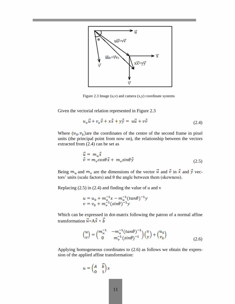
frames that can be seen in Figure 2.3:
- The first one, used to express the image coordinates (u,v), is given in pixel
coordinates and its location in the image planes is arbitrary. Here, as usual in
computer vision literature, the origin of the image coordinate system is in the
upper left corner of the image array, but this is a common agreement and can
be changed by the user.
- The second one is an ortonormal system whose origin is in the principal
point of the image and with one of its vectors parallel to the other system. Its
coordinates are called normalized coordinates (x,y).
The relationship between the coordinates in both systems must be obtained as
the next step of the transformation.
11
Figure 2.3 Image (u,v) and camera (x,y) coordinate systems
Given the vectorial relation represented in Figure 2.3
(2.4)
Where ( are the coordinates of the centre of the second frame in pixel
units (the principal point from now on), the relationship between the vectors
extracted from (2.4) can be set as
(2.5)
Being and are the dimensions of the vector and in and vec-
tors’ units (scale factors) and θ the angle between them (skewness).
Replacing (2.5) in (2.4) and finding the value of u and v
Which can be expressed in dot-matrix following the patron of a normal affine
transformation =A +
(2.6)
Applying homogeneous coordinates to (2.6) as follows we obtain the expres-
sion of the applied affine transformation:

12
Which represents (2.6) as follows:
(2.7)
This is the transformation between the coordinates in both reference frames in
the image plane, so if we add (2.7) to the conical projection expression (2.1),
we get the matrix that relates the 3D normalized coordinates of a real point
(referred to the camera reference frame) to the pixel coordinates of the pro-
jected point in the image plane, whose expression is given by (2.8)
(2.8)
- The intrinsic parameters
The elements contained in the K matrix in (2.8) let us relate the coordinates in
the camera reference frame (normalized) with those in the image frame (in
pixel). They are called intrinsic parameters of the camera, and K the intrinsic
matrix, that can be written as follows
Where αu= f/mu and αv= f/mv express the relation between the focal length
and the coefficients mu and mv used to change the metric units to pixels.
2.2.3.3 Change of basis from the camera reference frame to the real object reference
frame
Generally, the 3D points are referred to a reference frame different from the
camera frame, the world reference frame. Both systems are related through a
Euclidean transformation (translation and rotation) as represented in Figure
2.4.

13
Figure 2.4 Transformation between the camera and the world reference
frames
Therefore, knowing the coordinates of the point in the world reference frame
and the coordinates of the same point referred to the camera reference
frame , the relationship between them can be expressed as
where the vector contains the coordinates of the optical
centre of the camera in the world reference frame and the matrix R represents
the rotation of the camera coordinate system with respect to the world system.
Once again, expressing this equation in homogeneous coordinates we obtain
(2.9)
-The extrinsic parameters
The Euclidean transformation between frames is defined by the matrix He in
(2.9), which contains R and t, called the extrinsic parameters of the camera.
2.2.4 Matrix of complete projection
Once the process of formation of the image is completed, the equation that
models the mapping between the real point in the world reference frame and
its projection in the image reference frame is given by the complete projective
matrix showed in (2.10)
(2.10)
This matrix contains all the information concerning the conical projection and
the intrinsic and extrinsic parameters of the camera and let us solve (2.2) as
follows
(2.11)

14
2.2.5 Lens distortion
In the last step we have worked with the assumption that the linear pinhole
model of the camera is accurate enough for the process of formation of the
image. The 3D points, the image points and the optical centre were collinear
so the lines in the real world were projected as lines in the image plane. How-
ever, a real lens (especially low quality lens) cannot be considered as perfect
since they introduce systematic deviations in the linear model that must be
taken into consideration. The corrections for these distortions in the image
coordinates given by (2.13) and (2.15) can be added to the pinhole model giv-
en in (2.11) in order to reach a better accuracy and keep working with the lin-
ear model (Heikkila & Silvén, 1997). These corrections must be applied in the
right step of the image formation process, during the initial projection of the
object in the image plane, which means that they will be performed in normal-
ized coordinates, as can be seen in the appendix A.7.
The most common distortion types, and the ones applied in this project, are
radial and tangential distortion, whose consequences are showed in Figure
2.5. These both components are going to be added to the pinhole model in or-
der to obtain an accurate calibration and are usually expressed as (2.12)
(2.12)
Where are the distorted coordinates, (x,y) the ideal (distortion-free)
coordinates and , are the components of the radial and tangential distor-
tion.
Figure 2.5 Consequences of the lens distortion
2.2.5.1 Radial distortion
The radial distortion causes the actual image point to be displaced radially in
the image plane, and it is modelled in (Hartley & Zisserman, 2000) as follows
(2.13)

15
Where and is a Taylor se-
ries expansion around the centre (r=0), whose coefficients ki are obtained as
part of the calibration process to correct the distortion. They are considered as
a part of the intrinsic parameters of the camera. If the impair coefficients of
are eliminated, the polynomial is differentiable in the origin, which is a
better approximation for a real world description, although this depends on
the authors.
In this project, k2, k4 and k6 are used to compensate the radial distortion
(Bouguet, 2009), so (2.13) turns into
Assuming that the centre of the radial distortion does not coincide with the
principal point, which is our case, the model (2.13) would be modified to
(2.14)
(2.14)
And r would be calculated consequently as
This is due to the fact that centres of curvature of lens surfaces are not always
strictly collinear, which causes decentering distortion and creates the second
component of distortion, the tangential.
-Kinds of radial distortion
The most frequent kinds of radial distortion are barrel and pincushion. In the
Figure 2.6 two examples of them modelled by a polynomial of three coeffi-
cients with centre in the principal point are showed.
Figure 2.6 Barrel and pincushion distortion examples

16
2.2.5.2 Tangential distortion
This second component of the distortion, as explained before, is caused by
physical elements in a lens not being perfectly aligned.
The expression for the tangential distortion component is written in the fol-
lowing form by (Hekkilä & Silvén, 1997)
(2.15)
Where p1 and p2 are the coefficients for tangential distortion.
2.3 CALIBRATION PROCESS
2.3.1 Introduction
The camera calibration process is a necessary step in order to obtain three-
dimensional information from 2D images of the scene. Several different tech-
niques based on photogrammetry and auto-calibration exists, and as the result
of them, we obtain the intrinsic and extrinsic parameters of the camera model,
that describe the mapping between 3-D reference coordinates and 2-D image
coordinates. The overall performance of our machine vision system will
strongly rely on the accuracy of the calibration. This is why the process must
be carried out with the guarantee that the results are as similar to the real pa-
rameters as possible, which means that both the calibration method and the
way it is applied must be chosen regarding our application and the resources
we have in order to be optimum.
2.3.2 Calibration methods
2.3.2.1 Explicit camera calibration
The explicit methods are those where the camera model is based on physical
parameters, like focal length and principal point. Physical camera parameters
are commonly divided here, as explained, into extrinsic and intrinsic. As a re-
sult of the explicit calibration methods, the components of the model have a
physical meaning and can be easily related to real camera parameters.
2.3.2.2 Implicit camera calibration
In general is not possible to estimate the physical parameters separately so the
components of the projective matrix generally have no physical meaning,
which is our case. The parameters obtained during the calibration process,
their meaning and the notation utilised will be explained in the next point.

17
2.3.3 Obtaining the projection matrix
Given a known set of 3D points Pi and a corresponding set of points in the
image pi, we have to calculate the projection matrix M of the equation (2.2).
Taking into consideration the existence of noise in the images, this equation
cannot be exactly resolved, so the matrix M will be searched in order to adjust
the projections of Pi to the points pi as accurate as possible.
A two-step method, in which the initial parameter values are computed linear-
ly and the final values are obtained with nonlinear minimization, is going to
be applied to resolve the process. (Viala & Salmerón, 2008)
2.3.3.1 First step: Linear parameter estimation
The direct linear transformation (DLT) method (Abdel-Aziz, & Karara, 1871)
is based on the pinhole camera model, and it ignores the nonlinear radial and
tangential distortion components.
The coordinates of the projected point in the image are obtained through the
intersection of three planes as showed in Figure 2.7
Figure 2.7 Linear projection in the image plane
The three planes are the image plane π1 and two others, π2 and π3, which are
defined by the point P and the optical centre and whose mutual intersection
defines the line that contains p. The intersection of this line with the image
plane is the projection pi of the point Pi in the image.
Since two points are not enough to define the planes π2 and π3 the number of
possible planes is infinite. If we take those two whose intersection with π1 is a
parallel line with one of the vectors of the image coordinate system , as
shown in the figure, the position of both intersections in the image will give
us the row and the column of the projected point p(u,v).

18
The projection in 2.8 can be represented as follows
(2.16)
The image projection process can be generally formulated as a calculus of a
homography but in different dimensions making use of the projection matrix
M
(2.17)
Now the components of M, as explained, do not have any physical meaning.
In order to obtain the parameters of the matrix M, (2.17) can be reformulated
and expressed as dot matrices
(2.18)
During this first step of the implicit camera calibration, a set of N points will
be acquired from the images of the pattern, which will result in a system of
2N equations Am=0
19
This system must be resolved in order to get the set of parameters mi for
(2.16). The set of images points pi are obtained as observed values (not ideal)
in the images acquired for the calibration, and are used to solve the system by
a least-squares method.
Considering the presence of noise in the set of points pi, there is not vector m
that verifies Am=0 but Am=ε being ε the error vector. The norm of this error
vector must be minimized to optimize the solution
Now the system Am=ε can be seen as an eigenvalues problem for B=ATA,
where the eigenvector related to the smallest eigenvalue must be found in B in
order to obtain mi.
2.3.3.2 Second step: Nonlinear parameter estimation
The main disadvantages that the direct methods involve produce that the ob-
tained calibration results are not accurate enough for real applications in the
presence of noise (Hartley & Zisserman, 2000). These problems are the lack
of the lens distortion effects correction in the process, and the fact that the
constraint in the intermediate parameters of the algorithm is not consider
since the aim is creating a non-iterative algorithm. The geometric error in an
image can be defined as (2.19)
(2.19)
Which is the error between the points in the image (real) and the points pro-
jected as MPi. If we assume that the error in (2.19) is white Gaussian noise,
then the best estimated matrix M is the one that minimizes the residual be-
tween the set of N observed points and the expected points
(2.20)
The least-squares estimation technique can be used to minimize (2.20). Due to
the nonlinear nature of the camera model, simultaneous estimation of the pa-
rameters involves applying an iterative algorithm. For this problem the Le-
venberg-Marquardt optimization in (Levenberg, 1944) and (Marquardt, 1963)
has been shown to provide the fastest convergence. However, without proper
initial parameter values the optimization may stick in a local minimum and
thereby cause the calibration to fail. This can be avoided by using the parame-
ters from the DLT method as the initial values for the optimization.

20
2.4 CAMERA CALIBRATION WITH MATLAB TOOLBOX
2.4.1 Patterns for calibration
Currently there are many methods that make use of different kinds of planar
patterns since any characterized object can be used as a calibration target, as
long as the 3-D world coordinates of the target are known in reference to the
camera. Furthermore, there are some other techniques that perform the cali-
bration without them. Here we focus on the two basic ones, Tsai’s and
Zhang’s methods.
2.4.1.1 Tsai’s calibration method
Tsai’s method (Tsai, 1987) is a classic example of calibration based on the
measures of the coordinates of the 3D pattern’s points (Figure 2.8a) referred
to a fixed reference point. This method has been widely implemented in the
past century, and has been proved to supply the best results provided that the
income data have been taken with a very high level of accuracy and low
noise, conditions unreachable in this project.
2.4.1.2 Zhang’s calibration method
This technique, explained in (Zhang, 1998), unlike the other one, uses the co-
ordinates of the points situated on a 2D planar pattern as the one in Figure
2.8b. In this way, the calibration is more flexible due to the fact that the cam-
era and the pattern can be freely moved and as many images as desired can be
taken, without needing neither to measure the planar pattern again nor to
know the motion. Furthermore, with Zhang’s method the pattern does not re-
quire a special design and can be hand-made.
Figure 2.8 3D and 2D patterns for calibration

21
2.4.2 Calibration with planar pattern
As explained, planar checkerboard patterns are the easiest to calibrate with,
because they do not require very high level of accuracy and low noise in the
inputs, and the initial estimation of the homography between the pattern and
the image plane can be solved easily as explained in (Zhang, 1998).
Knowing the relationship between the 3D points and its image projection
through M, expressed in (2.2)
Without loss of generality the assumption that the plane pattern is situated in
Z=0 in the world coordinate system, as showed in Figure 2.9, is made.
Figure 2.9 Location of the world coordinate system in the 2D pattern
If the matrix M is factorized in (2.2) separating the intrinsic and extrinsic ma-
trices
(2.20)
And the columns of the rotation matrix are denoted as ri, (2.20) is expressed
as follows
Since Z is always equal to 0, a point Pi and its image pi is related by a homog-
raphy H
with H=

22
2.4.3 Camera calibration toolbox in MATLAB
With this last assumption, the 3D coordinates of the corners in our planar pat-
tern can be easily obtained from the set of images acquired with our cameras,
so the utilized MATLAB toolbox has all the inputs needed to solve the rota-
tion and translation vectors that relate the left and right cameras as well as the
intrinsic camera parameters. The calibration method implemented in this
toolbox is partially inspired in Zhang’s method, with differences in the esti-
mation of the internal parameters, and makes use of the Heikkila and Silven
distortion model including two extra distortion coefficients for tangential dis-
tortion.
The toolbox has been developed for MATLAB 9 (Bouguet, 2009) and is
based on the OpenCV implementation developed in the C programming lan-
guage. The MATLAB version was chosen based on the ease of use and better
performance; the OpenCV implementation utilizes an automatic corner finder
without any user input, which was found to be unpredictable at finding cor-
ners, with performance dropping drastically as the camera was moved further
from the calibration target. This method appeared to be tailored for close
range calibration, which is not our case.
2.4.3.1 Calibration procedure
The steps in the calibration procedure based on a plane calibration target with
the MATLAB toolbox are the detailed in (Viala & Salmerón, 2008):
- Creation of a 1x1m chessboard of 10x10 squares. It can be seen in the
Figure 2.10. Only the 8x8 internal squares have been used for the calibra-
tion, being a high enough number.
- Acquisition of 30 images of the pattern with both cameras at the same
time from multiple views. The images have been acquired trying to make
the chessboard occupy the most of the images, with its centre in the centre
of the images. After several trials, a number of images between 25 and 30
has demonstrated to be the optimal with this toolbox.
- Automatic detection of the corners by the system once the perimeter of the
board has been selected manually, with an initial guess at radial distortion
if needed.
These steps provide the necessary inputs to the toolbox for the stereo calibra-
tion performance. During this procedure, the estimation of the skew has been
added to the algorithm, three images with a high lens distortion have been re-
moved from the set of 30 and the estimation of the sixth order polynomial for
the correction of the distortion has been set in the search of the best results
achievable with the two webcams.

23
Figure 2.10 2D pattern for the calibration
2.5 BINOCULAR VISION
The binocular human vision takes 2D images from two different points of
view (as showed in Figure 2.11) and makes use of the information contained
on them (disparity) to develop a three-dimensional picture in which the depth
of the objects can be resolved by stereopsis (Howard & Rogers, 1995).
This impression of depth extracted from the binocular disparity depends on
the distance between the eyes. A greater distance involves a bigger disparity
so the depth perception is better for distant objects, and the equivalent for a
smaller distance and closer objects. The equivalent to this distance in our pro-
ject is the baseline between the cameras.
Figure 2.11 Human vision system
The machine vision system designed in this project has used the human vision
system basis as reference although there are other methods to extract infor-
mation of the depth range with just one camera, via structured light or time of
flight techniques, that are not the matter of this project.

24
2.6 STEREO VISION
2.6.1 One camera systems
The stereo vision is a technique aimed at inferring depth from two or more
cameras which is nowadays a wide research topic in computer vision. Since
we need to calculate the exact 3D location of the target in our visual servoing
system, the solution unavoidably passes through a stereo vision system.
With one single camera we are able to get the projected point of a real one in
our image can be seen in Figure 2.12.
Figure 2.12 Linear projection in one camera
But since both real points (P and Q) project into the same image point (p ≡ q)
in 2.13, for each collinear point along the same line of sight, we cannot differ-
entiate between those that are located closer or further from our optical centre.
As a result of this, optical illusions like the one in Figure 2.13 are created that
prevents us from being able to work out real distances and geometries.
Figure 2.13 Optical illusion in one camera systems

25
2.6.2 Two cameras systems
With two (or more) cameras we can infer depth, by means of triangulation
since a second camera adds the needed equations to solve the system in (2.18)
without any assumption about the situation of the world reference frame.
As said, the bases of the use of two cameras are the human vision system and
its design.
Figure 2.14 Linear projection in two cameras systems
2.6.3 Triangulation
The triangulation consists in finding the position of a 3D point Pi given its
homologous projections in two images pi and p’i and the projection matrices
of both cameras M and M’ (Hartley & Sturm, 1997). However, the existence
of noise in the image coordinates, as shown in the Figure 2.15, difficulties the
process since the reprojected lines will not intersect in the space, which makes
necessary an approximation.
Figure 2.15 Triangulation with pixel noise
2.6.3.1 Linear triangulation
The process here would be equivalent to the one developed to obtain the pro-
jection matrix in the calibration. Given the homology between the two pro-
jected coordinates of the point in both images we obtain the relationship be-
tween the 3D coordinates and the projected ones through the equation (2.16).

26
But now, since we have two cameras, the system has four equations with
three unknown factors (X, Y, Z), so it can be resolved and the 3D coordinates
of the point found, following the same procedure based on the eigenvalues
problem.
2.6.3.1.1 Uncertainty
The reconstruction of the 3D points will be more reliable with a wider angle
between the projected lines through the projections of the same point in both
images, as it can be seen in the Figure 2.16. The dark zone in the figure repre-
sents the zone of uncertainty, which depends on the angle between the lines.
Figure 2.16 Uncertainty in the reprojection
In our system, this factor will have to be kept in mind during the calculus of
the baseline between our two cameras. However, the limit for the baseline
will be the overlap in the field of view of the cameras required to model the
robot workspace, as it will be explained in the next points.
2.6.3.2 Correspondence problem
The correspondence problem refers to finding the homologous point in one
image once we have the first point in the other image. The differences be-
tween both images can be due to the movement of the camera or the fact that
the images of the same object have been acquired with two different cameras,
which is our case. Here, the steps in the resolution of the stereo correspond-
ence problem are introduced in order to be implemented in the algorithm de-
veloped in MATLAB for our application.

27
2.6.3.2.1 Estimation of the homography
A 2D homography between a couple of images describes the projective trans-
formation that takes each point pi(u,v) from one image to its correspondent
point pi’(u’,v’) in the other as explained in 2.4.2
The matrix H3x3 is the matrix of the 2D homography.
The process of obtaining the matrix H shares many characteristics with the
described in the estimation of the projective matrix (which can be seen as a
homography 3D-2D), so it is not going to be repeated here.
2.6.3.2.2 Matching
Since in our project the number of pairs of points to relate is going to be one,
which is the centre of gravity of the target to track, a technique must be found
in order to find without doubt the correspondence between the points in both
images as fast as possible, due to the fact that it is an on-line step of the algo-
rithm. This problem is known as matching, and consists in finding the corre-
spondent points in both images via segmentation techniques, in which similar-
ities between both images are searched or via edges’ correlation, among other
ways. These techniques look for areas with a small difference in both pictures,
assuming that the one with the minimum correlation error must contain the
homologous point.
The Figure 2.17 contains two images that show a typical problematic situation
in which feature detection does not guarantee a correct result.
Figure 2.17 Challenges in matching process by segmentation
But regardless the technique used, this process is heavy and time consuming
since it should be carried out in the whole image, as well as not accurate
enough due to the fact that depends strongly on the features of the objects in
the images acquired.

28
2.6.3.2.3 Epipolar constraint
The solution to the matching problem goes through the use of the epipolar.
The epipolar constraint states that the homologous point (p’) of the projection
of P over the first image plane (p) must be in the projection of the line that
contains the optical centre of the first camera and P over the second image
plane, which is the epipolar line of p (e2).
Figure 2.18 Epipolar geomatry
The Figure 2.18 shows the explanation given below. Basically, the epipolar
constraint avoids needing to use 2D search domain of the images during the
matching procedure, saving time and processing capacity. Now the search of
the smallest correlation error between the two images can be carried out
through the 1D domain, as showed in the example in Figure 2.19
Figure 2.19 Matching through the epipolar line
Notwithstanding, the presence of noise in the coordinates prevents us from
applying a search only through the epipolar line. Assuming that the projected
coordinates can contain an error, the field of search in our application has
been widened enough to ensure that the homologous points are found.
29
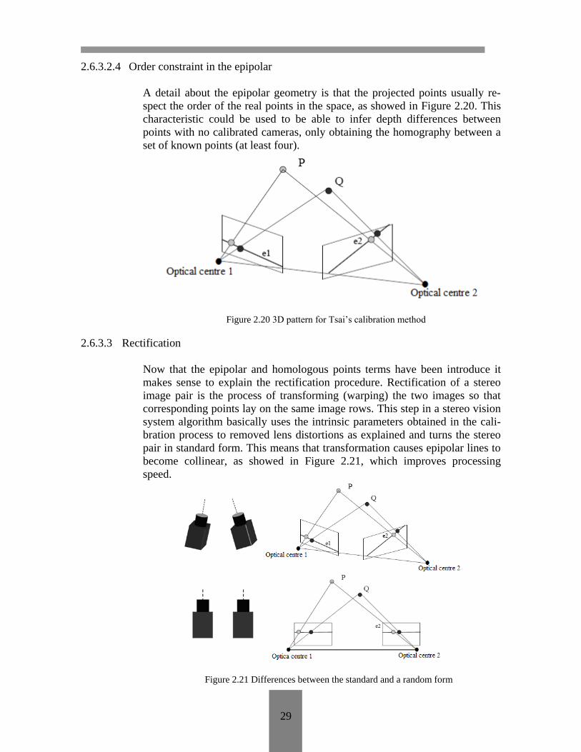
2.6.3.2.4 Order constraint in the epipolar
A detail about the epipolar geometry is that the projected points usually re-
spect the order of the real points in the space, as showed in Figure 2.20. This
characteristic could be used to be able to infer depth differences between
points with no calibrated cameras, only obtaining the homography between a
set of known points (at least four).
Figure 2.20 3D pattern for Tsai’s calibration method
2.6.3.3 Rectification
Now that the epipolar and homologous points terms have been introduce it
makes sense to explain the rectification procedure. Rectification of a stereo
image pair is the process of transforming (warping) the two images so that
corresponding points lay on the same image rows. This step in a stereo vision
system algorithm basically uses the intrinsic parameters obtained in the cali-
bration process to removed lens distortions as explained and turns the stereo
pair in standard form. This means that transformation causes epipolar lines to
become collinear, as showed in Figure 2.21, which improves processing
speed.
Figure 2.21 Differences between the standard and a random form

30
The cameras’ standard form imposes the cameras to be aligned and with the
same focal length. In our system the cameras have been placed like this so we
can avoid carrying out the rectification in order to save processing time.
2.6.3.4 Summary of the chapter
Following the described steps, the desired homologous projected points of the
centre of gravity of our target in both acquired images are obtained. Then,
they are used to calculate the vector that defines the position of the target in
the left camera reference frame, assumed as our world coordinate system, by
means of triangulation. In order to do so, an algorithm has been developed in
MATLAB that has as inputs the results of the stereo calibration performed
and the two acquired images and as outputs the relative vectors of the position
that will guide the movements of the TCP of the robot in its equivalent refer-
ence frame. It follows that there must be an overlap in the two images so that
a point in the left image also exists in the right image and a correspondence
can be found. To guarantee this, the baseline between our cameras, their situa-
tion in the space and the illumination system has been worked out carefully
considering the robot workspace.
2.7 PARAMETERS OF THE STEREOVISION SYSTEM
The next steps in the design of the machine vision system, used to track and
extract the position of the target in the Cartesian space, have been carried out
taking into consideration these main points:
- The quality and features of the cameras utilized.
- The kind of robot that is going to be controlled, its morphology, size, the
model and its motion features.
- The processing hardware available.
- The illumination resources.
- The environment of the system as a source of electrical noise.
2.7.1 The Logitech HD Webcam C270
The cameras that we have been given for this project are two webcams C270
HD of Logitech with USB 2.0 connectivity interface, showed in Figure 2.21.
Its relevant features for the application can be found in its datasheet
Focal distance 4mm
Field of view (FOV) 60 degrees
Frames per second (max) 30fps
Optical resolution 1280 x 960 1,2MP
Length of the connection cable 1,5m

31
Figure 2.21 Logitech HD webcam
The size of the sensor in the camera can be obtained from its parameters
through the equation 2.21, obtained from the Figure 2.22
Figure 2.22 Calculus of the size of the camera sensor
(2.21)
This formula must be applied for each side of the sensor with the respective
angle of the field of view since our sensors are rectangular.
These cameras are not designed for this kind of use, therefore they present a
poor quality concerning their lens and resolution (that can be seen in terms of
the high distortion) and the focal distance cannot be changed. These facts will
play an important role in the design of the structure of the system and will
greatly influence the results of the triangulation.
Another important matter is that the cameras must be returned to the laborato-
ry once the project is finished, so they cannot be fixed permanently to the arc,
which will result on an important lack of robustness in the system since a
small relative movement between them will involve the whole repetition of
the calibration process.

32
2.7.2 The location of the cameras
The cameras must be placed in order to model the workspace of the robot in
their overlapped field of view. In this way, we guarantee that all the equiva-
lent points within the robot workspace can be reached by the user with the
target in FOV, so we do not limit the movements of the robot. Keeping this in
mind, the best location for the cameras seems to be over an arc pointing to the
floor.
A vertical configuration lets us specify the available depth range as well as
keep under control the objects in the cameras field of view easily. Further-
more, it is known that the biggest errors during the target tracking are going to
be in the triangulation of the Z coordinates. By placing the cameras in an arc,
we choose the Z coordinate in the camera reference frame to be the same than
in the original robot coordinate system (but inverted), which means that the
movements of the robot in the X and Y axis will be more accurate than in the
Z axis. Finally, in order to correct this inversion between the reference
frames of the left camera and the robot, we have defined a new coordinate
system for the robot equivalent to the camera’s one in situation and orienta-
tion, so the output vectors of the machine vision system do not need to be
transformed before being sent to the robot. This point will be explained more
deeply in the fourth chapter.
2.7.2.1 Dimensions of the arc
The problem of obtaining the best arc measures and cameras baseline has as
inputs
- The workspace of the model of robot we are going to work with. It can be
seen in the Figure 2.23.
- The angle of the FOV of the cameras, which cannot be modified since the
focal length is fixed in this model.
- The condition that the cameras must be placed in a standard form. The
reasons for this condition are two:
+We want to avoid the rectification step during the processing to
make the algorithm faster.
+We are not allowed to fix the cameras permanently to the arc,
which makes more difficult to find a different configuration for
them and keep it.
The IRB 120 robot of ABB has as maximum height 982 mm and a diame-
ter of 1160mm around the centre of its base. These are the measures we
need for the design.

33
Figure 2.23 IRB 120 workspace
The cameras have an angle of the FOV equal to 60 degrees, which means
that in a standard configuration the overlapped FOV will also have an an-
gle of 60 degrees and the same shape. Let’s assume that the robot’s work-
space is a sphere with diameter D= 1.3m tangential to the floor in the cen-
tre of the robot base, and that the overlapped field of view can be seen as a
pyramid, that must involve the sphere as showed in Figure 2.25
Figure 2.24 Assumptions for the calculus of the overlapped zone
The rectangular base of the pyramid has a long side given by
And its height depends on both the height of the arc and the baseline
between the cameras. During the resolution we have kept in mind that a
wide baseline could facilitate the triangulation as explained, but the limit
here is set by the volume of the sphere, that cannot be modified.

34
The best solution achieved for the problem is showed in the scheme in
Figure 2.25 (in mm)
Figure 2.25 Measures of the arc for the cameras
The arc will have a height of 2000 mm and the baseline of the cameras
will be 70 mm in order to cover the sphere that models the workspace of
the robot.
The Figures 2.26 and 2.27 show the final configuration of the real arc and
the cameras once installed.
Figure 2.26 Configuration of the cameras for stereo vision

35
Figure 2.27 View of the final design for the arc with the cameras
2.7.2.2 Range resolution
With the chosen baseline and the current focal length of the cameras we
are able to obtain the resolution in the depth measures taken by the system
for our depth range (2-1.1m) through the next equation. We just need to
know the pixel increment (Δd) for a depth increment (ΔZ) in the image
2.7.3 Illumination
Although the illumination can play an important role in the success of a
machine vision system in general, since we have not resources to provide
the system a proper illumination, the best available option has been
placing the arc with the cameras directly under the illumination field of
one of the lamps in the laboratory. Proceeding this way, we simulate a
bright-field illumination system, in which the white light transmitted from
below the cameras will increase the contrast between the target and the
environment, making the detection easier.
Figure 2.28 Bright field illumination scheme

36
The source of light is an incandescent lamp with planar geometry. It is
characterized by a low luminous flux but provides a good luminous
intensity with a strong diffused component and a weak specular
component. The lamp as well as its position with respect to the cameras
can be seen in the Figure 2.29.
Figure 2.29 View of the final illumination configuration
2.7.4 Structure of the system
The scheme of the tasks performed by the machine vision system
involves, as explained, the acquisition of the images, their processing by
the developed algorithm and the communication of the extracted
information.
Figure 2.30 Scheme of the tasks in our MVS
In this description, showed in Figure 2.30 we do not consider the software
tools or hardware devices that carry out these tasks. However, in function
of their hardware components, a system that implements the scheme
showed above can be classified as follows (Xu, 1981).

37
a) PC-based vision system
In a PC-based vision system the image processing is implemented in the
CPU of a computer, which will provide the memory space we need and
the I/O modules for communications as well as the power supply for the
whole system. A general scheme of this kind of MVS is showed in Figure
2.31.
Figure 2.31 PC-based vision system
b) Embedded vision system
An embedded system as the one in Figure 2.32, would provide image
sensing, processing and features extraction and outputs image features
directly integrated in a processor, which makes this kind of systems
lighter than the other one but with a weaker computing capability.
Figure 2.32 Embedded vision system
2.7.4.1 Hardware components of the PC-based system
The images obtained by our webcams are transferred to the computer via
the USB 2.0 interface supported by the cameras. The computer processes
the images and stores the outputs in a common file that can be accessed by
the IRC5 robot controller through an Ethernet connection. This kind of
system is large and heavy but provides more storage and processing
capacity than the embedded systems. A basic scheme of the PC-based
system can be seen in Figure 2.33.

38
Figure 2.33 Scheme of our PC-based MVS
Since the transmission of the images is made through two 1.5m wire, it
has been considered as a possible noise receptor in the system due to the
fact that the environment in which the system is installed is an electrical
devices laboratory. Although some ideas related to shield the cables have
been thought, the idea was finally discounted.
The PC is a DELL model with an intel i5 processor and works with
Windows 7, which is a requirement of the webcams, with the version
Ultimate.
The robot controller, the compact version of an IRC5 for small robots,
belongs to the fifth generation of ABB’s robot controllers and its features
and applications will be explained in the fourth chapter.
2.8 ALGORITHM DEVELOPMENT
2.8.1 Introduction
The configuration of the cameras’ settings, the capture and image processing
algorithm, and the store of the process’ outputs in the memory to be sent to
the robot have been all performed in MATLAB 2014.a making use of the
Image Processing and the Image Acquisition toolboxes (Marques, 2011).
Tracking the target in the acquired images, analyze and pre-processing of the
images (filtering, segmentation, feature extraction, matching, etc)
triangulation and post-processing of the coordinates (filtering and correction)
are done by the MATLAB algorithm. The development of it has been carried
out focusing on low time consumption, as far as the faster the system is able
to extract suitable coordinates, the more real will be the control over the
robot. In order to do so, the design of the target and the environment in the
field of view, as well as the cameras collocation and configuration has been
thought trying to find the most suitable balance between robustness and speed
in our application.

39
2.8.2 Steps in the development
The following points contain the steps taken during the development of the
algorithm once the MVS has been completely designed. Despite the final re-
sults presented here, this process has been longer and iterative and other ideas
and steps were considered until the best results were achieved.
2.8.2.1 Design of the target
In view of the ideas that are leading the development of the algorithm, instead
of choosing a specific shape or concrete features for the target to be detected,
the final analysis will just involve color detection. This technique is faster and
does not require computationally intensive tasks, although it is also less robust
as far as it will need other white objects to be removed from the field of view.
However, the possibility to specify the minimum pixel size of the target that
the system is trying to track will prevent us from confusing the target with
smaller objects.
Figure 2.34 Model of white target used for tests
Therefore the target is going to be a white object, which can be chosen by the
user, with a specific size. In Figure 2.34, the target used for the tests is
showed.
2.8.2.2 Configuration of the cameras
The Image Acquisition toolbox provides the way to access automatically
detected hardware devices from MATLAB. The toolbox contains an adaptor
that provides a transparent interface between MATLAB and any frame
grabber or camera and also a Software Installer Pack, used to set up the
drivers needed to access our USB-based webcams through the adaptor. The
scheme of the connection can be seen in Figure 2.35.

40
Figure 2.35 3D Scheme of the the Image Acquisition toolbox
As it has been said above, the cameras have been configured to ease the target
tracking. The brightness, contrast and the parameters that define the camera
properties in general have been customized in both cameras making use of the
Image Acquisition toolbox of MATLAB showed in Figure 2.36. This toolbox
has also helped us establish the acquisition mode to be done in gray scale and
with the desired resolution.
Figure 2.36 Image Acquisition toolbox panel for Acquisition parameters

41
This configuration joined to the design of the white target (without specific
shape but size) has made possible to remove non-white objects from the
image avoiding that step in the pre-processing and the need of a specific
background. This lets the user of the system move the arms with the target
within the field of view of the cameras and place the whole structure
anywhere (except over white backgrounds).
Figure 2.37 Images from one camera before and after the configuration
The differences between the images given by the left camera in the arc before
and after the configuration can be appreciated in Figure 2.37.
The function 2 in appendix A encapsulates the cameras connections as two
objects that provides an interface for the acquisition performance in
MATLAB and configures them as explained to be used in the next functions
throughout the algorithm.
2.8.2.3 Capture and pre-processing of the images
Through the function 3 in appendix A, MATLAB is able to acquire images as
fast as the devices and the PC can support it. In our application, the acquisi-
tion time is 0.071 seconds in each camera. In order to enable this, the trigger
settings have been configured to use the system object generated by the func-
tion imaq.VideoDevice(). This function allows single-frame image acquisition
at a time from a video device (function step()). The system objects created by
the previous function are video input objects that represent the connection be-
tween MATLAB and a particular acquisition device. We work with this func-
tion instead of using videoinput() since it is more suitable for our application
work with discrete images than process video inputs. Furthermore, the
imaq.VideoDevice function offers different functions and properties more
proper for our aims that will be shown below.
Despite the low acquisition time required, the distance the target covers be-
tween the left and the right acquisition will be a source of errors during the
triangulation due to the fact that it will produce a wrong disparity.
42
This fact will automatically set a limit in the maximum speed the user can
move the target at, in order to avoid great errors. The produced error will also
depend on the distance between the camera and the position where the target
is being moved, since a longer distance will cause a smaller error in the dis-
parity.
The pre-processing performed over both images after the acquisition has been
reduced as much as possible in order to save time. After a binarization of the
gray scale images with a high threshold, the white objects that have passed
this step and are smaller than the specified size of the target are removed, re-
maining only the target if has been detected, or a black image in other case.
This method is also used to filter noise in the image.
In case there are white big objects within the field of view of the cameras,
they will cause an error during the next steps that can result in the loss of the
robot control, so this situation must be prevented. This is one of the weakest
points in the developed machine vision system, which can be solved by apply-
ing more robust and time consuming algorithms for detection, as explained.
2.8.2.4 Detection of the target
To locate the target in the input pre-processed images, the white areas in the
image are measured. If there is one bigger than the target’s size, is taken as
the target and the detection is considered as positive. In order to detect if oth-
er white, big objects are within the FOV and can result in a bad triangulation,
the number of white target-sized objects in the pictured is extracted, so if it is
greater than one, an error message is sent to the user and the triangulation is
not performed, otherwise, the process continues.
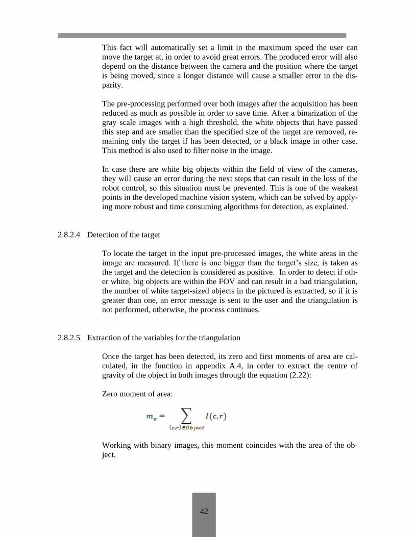
2.8.2.5 Extraction of the variables for the triangulation
Once the target has been detected, its zero and first moments of area are cal-
culated, in the function in appendix A.4, in order to extract the centre of
gravity of the object in both images through the equation (2.22):
Zero moment of area:
Working with binary images, this moment coincides with the area of the ob-
ject.

43
First moments of area:
Where c means columns in the picture and r means rows.
Known the relationship between the first order moments and the pixel coordi-
nates of the centre of gravity, these can be obtained as follows:
(2.22)
All the coordinates used in this procedure are given in pixels and are referred
to the image local reference frame located in the left upper corner as usual.
These are the inputs for the triangulation functions besides the intrinsic, ex-
trinsic and distortions parameters obtained in the stereo calibration.
2.8.2.6 Triangulation
This step computes the 3D position of the centre of gravity of the target given
the left and right image projections obtained in the last step. It makes use of
the outputs of the stereo calibration carried out before, proceeding this way:
a) Normalization of the coordinates
The normalized coordinates of the CofG are computed from the pixel coordi-
nates. The principal point coordinates, obtained during the calibration are di-
vided by the focal lenght and the skew is undone. After, if the lens distortion
has been taken into consideration during the calibration, which is our case, it
must be compensated. This task is implemented in the function 7 of the ap-
pendix A.
b) Correction of the lens distortions
The radial and tangential distortions are compensated through an iterative
method based on the distortion model from Oulu University. The two distort-
ed points in normalized coordinates are corrected making use of the constants
obtained during the calibration. The functions that perform the corrections are
8 and 9 in the appendix A.

44
c) Triangulation of the point in 3D space
With the projected coordinates of the target corrected and normalized, the tri-
angulation is resolved as explained and the real 3D coordinates referred to the
left camera reference frame are extracted with the function 6 of appendix A.
The relationship between the coordinates P in the left and right camera refer-
ence frames is given by (2.23)
(2.23)
Where T is a translation vector and R a rotation matrix that defines the trans-
formation between both systems.
In a perfect standard configuration of our cameras, the translation vector in
(2.23) would contain only the baseline and the rotation would be given by an
identity matrix as follows (mm)
However, the results from the stereo calibration are barely different due to the
fact that it was not possible to fix the cameras properly to the arc.
2.8.2.7 Post-processing
Taking into consideration that the process presented before is not perfect, the
generation of little systematic errors as well as greater random errors must be
considered too. In order to detect and correct or remove the wrong outputs ob-
tained from the stereo triangulation, three filters have been added to the algo-
rithm with the idea of preventing the robot from receiving wrong coordinates
that can destabilize the trajectories or result in unpredictable movements.
1) Filter of outliers points
This is the simplest filter, whose mission is check that the triangulated coor-
dinates belong to the workspace defined for the robot. If they are not within it,
they are removed. The workspace of the robot can be defined by the user to
adapt the programme to the placement of the robot.
This filter basically aims to detect and eliminate the outlier points caused by
random errors. The absolute coordinate’s vector referred to the left camera
reference frame that passes this filter is subtracted from the old absolute
vector which contains the current position of the robot.

45
As a result we obtain a new vector that contains the change in location or dis-
placement from the old point to the new one, specified by its magnitude and
direction .
Figure 2.38 Vector from current point A to next position B
2) Low-pass filter
This second filter works once the outliers have been removed. Its function is
to detect the maximum of the three components of the new displacement vec-
tor and compare it with the maximum advance per step allowed by the
user with the parameter R (mm). If this increment is bigger than R, the new
vector will be scaled down by multiplying it by a gain which will be inversely
proportional to the difference between R and the increment. However, if the
maximum increment in the coordinates is lower that R the gain factor (Kp)
will be equal one so the coordinates will not be modified.
Figure 2.39 Scheme of the low-pass filter
The aims of this filter are two:
- Reduce big unwanted changes in trajectories and instabilities that can be
caused by sporadic errors as well as by the pulse of the user and other
facts. This filter will not prevent these mistakes but will scale them down
so the loss of stability will be lower and the trajectories followed by the
robot will be smoother.

46
Figure 2.40 Example of a target trajectoy before and after filtering
In the symbolic cases in Figure 2.40, the first target trajectory would be
the ideal one, without neither human nor triangulation errors. This path is
in practice very difficult to get. The second path is the real one. Any kind
of possible errors after the first filter in the 3D coordinates have been add-
ed to the first model. The result of this is a steep trajectory which produc-
es an instable movement in the robot arm. The third trajectory is obtained
after applying the low-pass filter to the real one. The big changes in the
direction have been smoothed out so the result is closer to the ideal one.
- By limiting the maximum advance of the robot per new coordinates trian-
gulated, the user will keep a more real control over its movement even if
he is moving the target at a too high speed for the acquisition capacities.
As showed in the Figure 2.41, the system is going to divide the displace-
ment A to B into an n number of points Ai (where n=1, 2, 3,...i depends on
R), and at the end of each step (once the robot has reached the new posi-
tion given by ) it will check if the final trajectory of the target has
been changed by the user (from B to B’, i.e.) during the displacement
and it will act consequently. Therefore, the system will be able to
react to this change faster ( ) than if it had to wait for the robot to fin-
ish the trajectory and after performed .
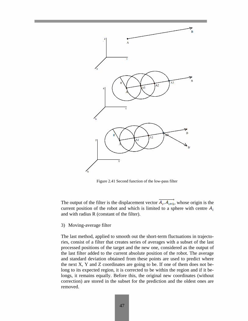
47
Figure 2.41 Second function of the low-pass filter
The output of the filter is the displacement vector , whose origin is the
current position of the robot and which is limited to a sphere with centre
and with radius R (constant of the filter).
3) Moving-average filter
The last method, applied to smooth out the short-term fluctuations in trajecto-
ries, consist of a filter that creates series of averages with a subset of the last
processed positions of the target and the new one, considered as the output of
the last filter added to the current absolute position of the robot. The average
and standard deviation obtained from these points are used to predict where
the next X, Y and Z coordinates are going to be. If one of them does not be-
long to its expected region, it is corrected to be within the region and if it be-
longs, it remains equally. Before this, the original new coordinates (without
correction) are stored in the subset for the prediction and the oldest ones are
removed.

48
The size of the subset (S) must be fixed according to our application, keeping
in mind that we want to avoid short-term fluctuation (related to triangulation
errors) but we do not want to lose or excessively delay long-term trends’
changes, which are real variations in the trajectory of the target made by the
user.
In order to initialize the filter, the first S triangulated points are not sent to the
robot but stored in the filter when the application is being started.
2.8.2.8 Communication
The architecture of the communication system, as well as the solution imple-
mented and the functions utilised in the robot controller will be more widely
explained in the third chapter. However, what must be detailed in this point is
the role that the communication function plays in the algorithm. The
MATLAB function can be seen in the point 5 of the appendix A.
The handshaking between the MATLAB algorithm in the computer and the
RAPID programme running in parallel in the robot is performed by the com-
munication application developed between both of them. In this synchronized
activity, the MATLAB algorithm acts as a producer, updating in the common
file the relative vector obtained as the output of the filters only when
the robot (the consumer) has acquired the last vector. This means that the
MATLAB process and the image acquisition system will only process a new
vector once the last one has been sent to the robot, which is the bottleneck of
the system, the element that will set the maximum speed of it.
2.8.3 Diagram of the algorithm
In Figure 2.42 the flow control diagram of the MATLAB algorithm is pre-
sented. The stages in the diagram represent the functions explained before in a
way that eases the understanding of the work flow followed by the algorithm.

49
Figure 2.42 Flow diagram of the MATLAB algorithm

50
3 COMMUNICATION INTERFACE
3.1 INTRODUCTION
This chapter contains the steps taken during the search and implementation of
a suitable communication interface between our MATLAB application in the
PC and the ABB robot controller. The problems we have faced during the
process, the implemented solution and its features and the reason for this
choice are explained in the next points.
It is convenient to remember here that the development of this communication
application has been parallel to the creation of the MATLAB algorithm,
concretely the communication function in appendix A.5, and the RAPID
application for the robot.
3.2 APPROACH TO THE PROBLEM
The idea in this part of the project is to set up a unidirectional data transfer
system able to send the vectors from the MATLAB application to the RAPID
program executed in the controller of the robot, respecting the timing and
with reasonable good features.
The factors that define the problem are listed below:
- The characteristics of the whole system: we have to define the sequence of
actions to perform and the flow control between the two hosts in the
system.
- The export possibilities in MATLAB 2014a: since the program developed
in MATLAB produces the vectors, we need to find the best way to work
with its outputs in other applications.
- The import possibilities in RAPID: the RAPID programming language for
applications in ABB robots has a set of instructions that can be used for
communications with the controller.
- The physical channels available for the transfer: the features of the robot
controller and the PC will set the possibilities for the connection between
source and receiver.
- The synchronization: since we have two tasks running in parallel we have
to find the most suitable way to make them join up.
3.3 PARALLEL COMPUTING
A parallel system is that in which more than one task is being carried out
simultaneously (Barney, 2007). Our system can be classified as a task-parallel
computer system since our applications in MATLAB and RAPID are running
at the same time in two different processors.

51
In any kind of computer system, a process is cooperative if it can affect or be
affected by the execution of another process, otherwise it is independent. In
our system, since we have two parallel applications executing and they have
to share resources in order to transfer data, they can be classified as
cooperative processes.
3.3.1 Producer-Consumer problem
The paradigm of cooperative process is the consumer-producer problem. It
describes two processes, the producer and the consumer, who share a
common fixed-size buffer used as a queue. The producer's job is to generate a
piece of data, put it into the buffer and start again. At the same time, the
consumer is consuming the data one piece at a time. This problem states
perfectly the situation in our system, in which the machine vision system can
be seen as the producer, that generates the vectors with the target position,
and the robot is the consumer that collects and applies those vectors in its
movements.
The scheme of this paradigm applied to our model can be seen in Figure 3.1.
Figure 3.1 Producer-consumer problem in our system
However, the paradigm specifies neither a real implementation of the
common buffer nor the size of it, which is what we must define in the next
steps of the chapter.
3.4 PROCESSES SYNCHRONIZATION
Concurrency in programming introduces some challenges that are not
considered in sequential programming, as managing common resources or
guarantying data integrity. They must be identified and solved here to
implement the producer-consumer paradigm.
3.4.1 Flow control problems
As our cooperative processes have to read and write shared data in a limited
common buffer, and the final result of the system (the robot’s movements)
will depend on the order they proceed, this situation produce race conditions.

52
There are two kinds of flow control errors that can be a result of the race
condition and that, therefore, must be prevented during the data transfer:
1) A same datagram is read twice by the robot. Although this kind of
situation would not cause any new movement in the robot, it could
involve a loss of time for the next actualization by the MVS and a slower
next movement.
2) A datagram is overwritten before being read by the robot. If a datagram is
lost, the robot trajectory losses the next point and will be less similar to
the real path of the target.
Both kinds of errors can be seen in the next images in Figure 3.2, where the
vertical lines represent the time of access to the buffer by both programs.
Figure 3.2 Flow control error while using a common buffer
The flow control problems could be avoided with an unlimited buffer, but this
would involve some other problems that will be explained in the next points.
In the context of race conditions two ideas must be kept in mind:
- Guarantee that both programs do not interfere in each other’s actions
when they are accessing the common resource
- Respect the handshaking between both process to prevent the flow control
problems
For implementing both requirements, a mechanism of mutual exclusion must
be established. This mechanism must control that when one of the process
accesses the common buffer, the other is not allowed to do it and must wait.
The section of code in which a programme accesses the common resources is
called critical section, which basically means that the race conditions can be
avoided if we control the entrance of the programmes in their critical sections.

53
3.4.2 Mutual exclusion
Considering the last ideas, both MATLAB and RAPID programs’ codes can
be divided into a critical section and another one in which they do not make
use of common resources, being always executed within an infinite loop, as
showed in Figure 3.3
Figure 3.3 Division of a program’s code for mutual exclusion mechanisms
Therefore, the mutual exclusion mechanism must be implemented in both
Entrance and Exit sections.
3.4.2.1 Strict alternation
The general rules for a common implementation of mutual exclusion
mechanisms in the producer-consumer problem are the following
- The consumer must wait for the producer to produce something if the
buffer is empty.
- The producer must wait for the consumer to consume something if the
buffer is full.
Since the tasks executed by the robot involve physical movements, it will
block the machine vision system execution until it finished its movements,
which makes it be the bottleneck of the system.
Owing to the last facts, the chosen algorithm for the mutual exclusion is a
strict alternation between the two processes. This is based on the state of a
common variable that determines what process is allowed to enter the critical
section. The process that is waiting for the permission is programmed to
repeatedly check the state of the variable, which is called busy-waiting.
Furthermore, with this algorithm, if one of the processes fails the other one
will be indefinitely blocked. This, which could be an inconvenience, turns
into an advantage here because in the presence of a failure the whole system
must stop for security to keep the robot arm under control.

54
3.4.2.2 Buffer size
Setting the size of the buffer to unlimited with two different program counters
would have avoided the control flow problems presented because any data
could have been overwritten or doubly read. However, the size of the buffer
has been set to one vector. The reason for this is that the possibility to store
more vectors in memory would have introduced a great delay between the
current movements of the target and the robot’s due to the big difference in
the speeds of both processes. Therefore, implementing an unlimited buffer
would have involved a loss of the real time control over the movements of the
robot. Furthermore, it entails memory space problems.
3.4.2.3 Semaphores
The chosen mutual exclusion mechanism for our implementation is the
semaphore. A semaphore is a common variable that is used for controlling
access, by multiple processes, to a common resource in a parallel
programming system. The binary type has two restricted values 0 and 1,
which means that the common resource only can be unavailable or available.
Here, the semaphores implemented are binaries, because the size of the buffer
has been set to 1.
The semaphores are equipped with two instructions to increase or decrease
their value that we situate in the Entrance and Exit sections in both programs.
These instructions must be atomic due to the fact that, otherwise, they could
be interrupted during the updating of the semaphores and the mutual
exclusion mechanism would fail.
The next is a pseudocode example of the algorithm implemented for the
producer-consumer problem in both sides of the line following the scheme in
Figure 3.3
process MATLAB() process RAPID ()
{ {
while (true) { while (true) {
XYZ = VectorExtraction(); decrement(semaphoreA);
decrement(semaphoreB); Target = ReadBuffer();
UpdateBuffer(XYZ); increment(semaphoreB);
increment(semaphoreA); Movement(Target);
} }
} }
The critical sections here are named UpdateBuffer() and ReadBuffer(), and
the rest of the code in each program contains the extraction of the target
position and the movement of the robot.

55
3.5 REAL IMPLEMENTATION
At this point, we have established the theoretical structure of our
communication system, the data flow, the paradigm and the mutual exclusion
mechanism. Now, the implementation must be solved. The possible
implementations of the system depend on the communication features that
both the PC and the robot controller have, so they must be deeply studied
here.
3.5.1 The IRC5 Compact controller
This ABB robot controller is analyzed here from the point of view of its
communication characteristics. A more comprehensive analysis can be found
in the fourth chapter.
The IRC5 supports the state-of-the-art field busses for I/O, sensor interface
functionality, remote disk access and socket messaging among others
networking features.
3.5.1.1 Machine interfaces
The machine interface options offered by this model of controller are listed in
the Table 3.1
Table 3.1 Avaible connections in the IRC5 compact controller
Inputs/Outputs Standard 16/16 (up to 2200)
Digital 24 DC or relay signals
Analogue 2x 0-10V, 3x 10V, 1x4-20mA
Serial channel 1x RS232 (RS422 with adaptor)
Network
Two channels
Ethernet (10/100 Mbits per second)
Service and LAN
Fieldbus Master DeviceNet
PROFIBUS DP
Ethernet/IP
Fieldbus Slave PROFINET
PROFIBUS DP
Ethernet/IP
Allen-Brandley Remote I/O
CC-link
Up to 6 channels
The distribution of the physical ports of the detailed communication features
in the controller console are showed in Figure 3.4

56
Figure 3.4 Frontal panel of the IRC5 compact
The existence of an installed Ethernet network in the laboratory makes us go
deeper, among the showed options, in the network capabilities of the
controller. Two Ethernet channels enable optimum separation of
communication tasks in the controller. The service port is dedicated for local
PC connectivity while the LAN channel is used for permanent connection to a
network for tasks such as program transfer monitoring, data collection,
operator communication, and field bus communication.
Table 3.2 Network capabilities in the IRC5 compact controller
Service and LAN Separate built in Ethernet channels
Fast communication 10 or 100 Mbit/s
Network file access The robot controller can host NFS (Network File Sys-
tem) or FTP (File Transfer Protocol) client software.
IRC5 file access The FTP server in IRC5 allows the controller to respond
to a request from an FTP client on a remote computer.
DNS Domain Name Server
Correlates device names to associated network IP ad-
dresses through a DNS server.
Allows the robot to access a network computer via a
DNS server to determine the network IP addresses of
other devices on the network.
DHCP Dynamic Host Configuration Protocol enables quick
connection to the network and IP addresses are obtained
automatically.
LAN channel (DHCP client software): The channel has
either a fixed IP address or it can be obtained from a
DCHP server on the network.
Service channel (DHCP server software): The channel
has a fixed IP address and can assign the connected PC
an IP address.
SNMP Simple Network Management Protocol Enables quick
access to control system network information.

57
The Table 3.2 contains the characteristics of the network capabilities in the
IRC5 Compact model.
Between the two available Ethernet channels, the LAN channel is chosen to
connect our PC and the controller, instead of creating a point-to-point
connection between our PC and the robot through the Service port. The
reasons are two:
- The MATLAB program that is being used here needs a network license
belonging to a different network in the university. To solve this problem, a
Virtual Private Network has been set up in our PC with a Citrix Receiver.
Due to the fact that the VPN works through public network, we need our
PC to be connected to Internet.
- Since this is the first time the utilized robot is connected to the network,
the communication system implemented in this project also aimed to
allow new communication applications in future projects for the robot
users. Focusing on this, it made sense to connect the robot not to one PC
but to the whole network.
In the view of these arguments, both the PC and the controller have been
connected to the Fast Ethernet network in the laboratory through two RJ45
connectors and the DHCP server in the network has automatically assigned
their IP addresses.
3.5.2 The remote PC
From the point of view of the computer, the only required feature is to have
installed the Internet protocol suite (TCP/IP) in order to be connected to the
network.
3.6 SOFTWARE
3.6.1 Network communications
At this point, an explanation about the kind of communication implemented
must be done. At the beginning of this project, the model of the robot we were
supposed to work with was the IRB 140, and its controller the S4Cplus. This
is an old model with a more limited set of communication features, and was
considering this model when the choice of the network configuration was
taken. Once we were offered to work with the IRB 120 and its IRC5
controller, the development of the idea was already started so we kept it.
Among its features, the SC4plus controller offered network file system
accesses using FTP/NFS client and FTP server.

58
Due to its simplicity, the Network File System (NFS) client software was
chosen to implement a remote mounted disk in the PC through our Ethernet
network, making use of the TCP/IP protocols as showed in the next diagram.
Figure 3.5 Second function of the low-pass filter
The protocols for to stablishment of the Network File System utilized by the
controller as showed in the Figure 3.5 are:
- IP: Internet Protocol provides a packet delivery service for TCP, UDP and
ICMP.
- ICMP: Internet Control Message Protocol handles errors and control
information between gateways and hosts in the network. These messages
are normally generated and handled within the TCP/IP networking
software.
- TCP: Transmission Control Protocol is a connection-oriented protocol that
provides a reliable full-duplex stream. TCP guarantees that the messages
reach their intended destination.
- UDP: A connectionless protocol. UDP does not guarantee that the
messages reach the indented destination. This has instead to be handled by
the overlaying protocols
- RPC/XDR: Remote Procedure Call/External Data Representation.
RPC is a protocol for invoking a procedure on a remote machine. For the
user of the RPC calls it appears like they are executed on the local
machine, i.e. the network is transparent.
XDR provides a standardized form for transmission of data between
different computers.

59
3.6.2 The Network File Sytem
NFS is a distributed file system protocol originally developed by Sun
Microsystems in 1984, allowing a user on a client host to access files over a
network through the IP protocol much like local storage is accessed.
In our system, the remote mounted disk installed allows the robot to access
the files stored on the PC hard disk C:\ making use of the NFS protocol.
These files will be used as the common buffer for the producer-consumer
problem implementation.
3.7 FINAL IMPLEMENTATION
3.7.1 The NFS server
A NFS server, haneWIN NFS server, has been installed in the external PC.
The haneWIN NFS software provides a simple and intuitive interface (in
Figure 3.5) to establish the characteristics of the server and set up the
exported directories in the mounted disk which will be accessible for the
robot.
Figure 3.6 haneWIN NFS server interface

60
The following are the tasks performed by the server during a normal NFS
execution:
- The server administrator determines what to make available, sharing the
names and parameters of directories.
- The server security-administration ensures that it can recognize and
approve validated clients throught their IP address.
- The server network configuration ensures that appropriate clients can
negotiate with it through any firewall system. This step was particularly
long as the firewall needed to be turned off from the register of the
operative system due to the settings of the network.
- The client machine requests access to exported data, typically by issuing a
mount command. The client asks the server which port the NFS server is
using, the client connects to the NFS server. The server has been
configured to not use the well-known ports in the computer and work over
the 8000.
- If all goes well, users on the client machine can then view and interact
with mounted file systems on the server within the parameters permitted.
3.7.2 The NFS client
In this point we explain the steps taken through the RobotWare option NFS
Client (scheme in Figure 3.6) in order to configure the controller parameters
that let it read and write to the remote PC in the same way as with its internal
hard disk:
- The application protocol must be configured to point out a directory on
the remote PC.
- The transmission protocol utilized must be specified.
- The physical channel that supports the transfer has to be chosen
Figure 3.6 Steps to stablish the NFS client in RobotWare

61
1) Defining the application protocol
This is a brief description of the system parameters used to configure the
application protocol.
Table 3.3 Parameters for the NFS application protocol establishment
Parameter Description
Name Name of the application protocol: “NFS client”
Type NFS
Transmission protocol For NFS is TCP/IP
Server address The IP address of the remote PC
Trusted This flag decides if this computer should be trust-
ed, i.e. if losing the connection should make the
program stop. In our application this is set to
“YES”.
Local path Defines what the shared unit will be called on the
robot. "pc1:” in our application.
Server path The name given to the exported folder on the re-
mote PC.
User ID Used by the NFS protocol as a way of authorizing
the user to access a specific server.
This parameter is not used here, so it has been set
to the default value 0
Group ID Used by the NFS protocol as a way of authorizing
the user to access a specific server.
This parameter is not used here, so it has been set
to the default value 0
2) Defining the transmission protocol
There is a configured transmission protocol called TCP/IP and no changes can
be made to it in the controller. It will make use of the IP address given by the
network DHCP server and its subnet mask. This is used by the NFS
application protocol, as explained in the last scheme.
3) Defining the physical channel
As explained, the physical channel utilized is one of the LAN connection in
the IRC5 controller. The available physical channels in the controller can be
found under the topic “Communication”, within the Type “Physical
channels”, where they can be given a name or new ones can be defined and
configured. Being an Ethernet port, no other features but the name have to be
established.

62
3.7.3 Semaphores in NFS
The binary semaphores implementation in the common file system has been
developed making used of .txt files as they were the shared variables. Two
primitives have been created both in MATLAB and RAPID programs to
create and delete two .txt files called “semaphoreA” and “semaphoreB” that
can be seen as the normal increase-decrease instructions for semaphores. Both
applications check the existence of their specified semaphore as if it was a 0-1
value in a common variable (here, delete=0, created=1), and depending on
this they create/delete the semaphore and proceed.
The programs created can be seen in appendix A.5 and B, and the
implementation in RAPID will be deeper explained in the next chapter.
3.7.4 Common buffer in NFS
The common buffer for storing the vectors is a .txt file called “Coordinates”,
so the instruction for the communication are simple write/read instructions in
MATLAB and RAPID, which is how the export/import problems in both
applications are solved.
3.7.5 Data frame
The only data transferred through the NFS application is a frame containing
the three components (X, Y, Z) of the output vector from the machine vision
system as follows
X:Y:Z
For future works, other control information can be added to the frame and be
shared through this file with only a few changes in the programming. Also a
feedback for the robot position could be implemented through this
communication system in order to set up a real control between the theoretical
position of the end-effector in MATLAB and the real one in the robot
controller. To do so, bidirectional transfer would be required, which would
involve higher time consumption and a decrease of the real time features of
the whole system. That is the reason why it has not been programmed in this
project.
63
4 PROGRAMMING THE ROBOT
4.1 INTRODUCTION
As it was said in the main introduction of this report, the final aim of this
project is the creation of an easy-to-use control system for the end-effector of
an anthropomorphic robot with six DOF.
In order to understand more deeply what the kind of element to be controlled
is and its characteristics, in this chapter a short introduction of the industrial
robots and manipulators, and their current definition is going to be presented.
The model of robot utilized as well as its controller is showed, with a small
presentation of the ABB programming language RAPID and the advantages
provided by RobotStudio. Furthermore, a very short explanation of the
process the robot follows to work out trajectories can be found. And finally,
the RAPID program developed in RobotStudio for the application is showed
in appendix B.
4.2 MANIPULATING ROBOTS
4.2.1 Industrial robot definition
The accepted definitions of the terms industrial robot and manipulator can
change depending on if they are used in the Euro-American market or in the
Japanese. For Japanese manufacturers, an industrial robot is any mechanical
articulated device aimed to manipulating tasks, while in the western market
the term involves higher complexity, especially concerning the control
(Barrientos et al. 1997).
The most widely accepted definition of industrial robot in the western market
is the given by the Robotic Industries Association (RIA) that states
“A robot is a reprogrammable, multifunctional manipulator designed to move
material, parts, tools or specialized devices through variable programmed
motions for the performance of a variety of tasks”.
This characterization, slightly modified, has been adopted by the International
Standards Organization (ISO) as
“An automatically controlled, reprogrammable, multipurpose manipulator
programmable in three or more axes, which may be either fixed in place or
mobile for use in industrial automation applications”.
In this description, the need for the industrial robot to have several degrees of
freedom is included.

64
Finally, one of the most complete definitions of the terms have been created
by the Association French Normalization Organization and Regulation
(AFNOR):
- Manipulator: “A manipulator is a mechanism generally composed of a
series of links, jointed between them, which aims to grasp and move
objects. It is multifunctional and it can be governed directly by a human
operator or through a logic device”.
- Robot: “An automatic servo controlled manipulator, reprogrammable and
polyvalent capable of positioning and orientating material, parts, or
special devices through variable reprogrammable motions/trajectories for
the performance of a variety of tasks.”
In view of these two last definitions, the industrial robot used in our system
should be now classified as a manipulator since we have stripped it of its
autonomy and now it is governed by a human, instead of automatically.
4.2.2 Morphology of the robot
Robots can be also classified attending their mechanical structure,
transmissions, sensors and actuators, control systems and end-effectors. Here,
we are especially interested in introducing the classification based on the
mechanical structure since it is the most relevant part while designing our
vision-based guidance system.
4.2.2.1 Mechanical structure
A robot is made up of a number of links joined by joints that enable relative
movements between consecutive links. The kind of joint will establish the
movement between links, existing six kinds of joints (Figure 4.1) with their
number of DOF
Figure 4.1 Kinds of joints in robotics

65
A degree of freedom in a joint is defined as the number of independent
movements that a link can do referred to the other link in the joint. The
number of DOF in a robot is set by the sum of the DOF of all the joints in it.
The most widely applied joints are prismatic and revolute, which means that
normally the number of DOF in a robot matches with its total number of
joints.
The different mechanical structures in a robot are a result of the different
joints configuration. The most common mechanical configuration in industrial
robots are showed in Figure 4.2.
Figure 4.2 Most common configurations in industrial robots
Taking into consideration that in order to completely specify position and
orientation in the space, six parameters are required (three for the position and
three for the orientation) if we want a robot to locate its TCP, we will
normally need six degrees of freedom.
4.2.2.2 Other characteristics
The quality of the robots regarding their performance can be measured not
only with their configuration and dimensions, but also with some features that
define the goodness on control of the motion and general behaviour while
moving.
- Payload capacity: weight of the load the robot is able to manipulate,
including the weight of the tool. This parameter depends on the size,
configuration and actuators of the robot. In some application the inertia
moments must be considered too while working out the payload capacity.
Generally, the payload capacity in robotics is given in diagrams like the
one in Figure 4.3, which expresses the distance from the TCP zero.

66
Figure 4.3 Payload in the IRB 120
- Resolution: minimum increment in the movement performable by the
robot controller. It is limited by the resolution of the encoders and the
A/D, D/A converters, the size of a word in the CPU and the actuators.
- Precision: average value after several cycles among the programmed
theoretical point and the reached one by the TCP. This precision is set by
the calibration errors, deformations and singularities in the calculus.
- Repeatability: radius of the sphere that contains the reached points by the
TCP after sending it to the same programmed point in equal work
conditions. Precision and repeatability are not related since a good
repeatability does not mean high precision and vice versa.
- Velocity: in the robot movements, it can be seen as link velocity or linear
average speed in the TCP. The velocity is related to other parameters due
to the fact that a high speed entails less precision and a lower payload.

67
4.3 ABB IRB 120
4.3.1 Description
The IRB 120 model (in Figure 4.4 the actual unit utilized) is an
anthropomorphic robot with six degrees of freedom and it is the smallest
multipurpose industrial robot by ABB manufacturer. It provides a high
precision and dexterity in its movements and good performance abilities
combined with a trim size and low weight.
Figure 4.4 IRB 120 utilized
4.3.2 Technical specifications
Table 4.1 Technical specifications of the IRB 120
Physical Dimension robot base 180x180 mm
Dimension robot height 700 mm
Weight 25 kg
Variants Reach 580 mm
Payload 3 kg (4kg with vertical wrist)
Armload 0.3kg
Features Position repeatability 0.01 mm
Robot mounting Any angle
Acceleration time 0-1 m/s 0.07 s

68
The Table 4.1 contains the relevant IRB 120 features for this application
The workspace of this model, defined by its maximum reach (without tool),
the configuration of its joints, its physical measures and its axis movements
(in Table 4.2), is showed in the images in Figure 4.5.
Table 4.2 Functional workspace of the IRB 120
Axis movements Working range Maximum speed
Axis 1 Rotation +165º to -165º 250 º/s
Axis 2 Arm +110º to -110º 250 º/s
Axis 3 Arm +70º to -110º 250 º/s 250 º/s
Axis 4 Wrist +160º to -160º 320 º/s
Axis 5 Bend +120º to -120º 320 º/s
Axis 6 Turn +400º to -400º 420 º/s
As explained, the volume that the robot can work in has been used to set the
measures of the overlapped FOV of the machine vision system.
Figure 4.5 Workspace of the IRB 120
4.4 IRC 5 COMPACT CONTROLLER
The IRB 120 is controlled by the 5th generation IRC5 compact (in Figure
4.5). This controller combines motion control, flexibility, usability, and safety
into a multi-robot controller with PC tool support. The IRC5 optimizes the
robot performance for short cycle times and precise movements.
Figure 4.5 IRC5 Compact controller

69
The IRC5 features the FlexPendant, which provides an intuitive interface
through a colour touch screen and a 3D joystick. The RAPID programming
language is used to communicate with the controller and create process appli-
cations to be performed by the robot. Remote robot monitoring is available
through standard communication networks, as explained before.
Among its other features, what interest here are the provided motion control
features. Based on advanced dynamic modelling, the IRC5 optimizes the per-
formance of the robot for the shortest possible cycle time (QuickMove) and
precise path accuracy (TrueMove). Together with a speed independent path,
predictable and high performance behaviour is delivered automatically, with
no tuning required by the programmer.
4.5 PATH GENERATION IN ROBOTICS
A shallow introduction is presented here of the robot kinematic control and
the procedure it carries out with the vectors the MVS sends in order to gener-
ate the trajectories that performs. For a deeper explanation about the direct
and inverse kinematics models and the dynamic model of a robot and kine-
matic and dynamic control, the lector is referred to (Barrientos et al. 1997).
4.5.1 Kinematic control
The kinematic control of a robot establishes the trajectories for each joint of
the robot while performing the user requests (final point, kind of trajectory for
the TCP, time, etc), regarding the robot dynamic limitations and kinematic
model and guaranteeing the goodness of the motion expressed by the parame-
ters explained.
Figure 4.6 Generic kinematic control diagram in a robot controller

70
The functions developed by the kinematic control are:
1) Create an analytic trajectory in the Cartesian space (evolution of each co-
ordinate as a time function) from the user program specifications.
2) Sample this continuous trajectory in N discrete points given by their posi-
tion and orientation (x, y, z, α, β, γ).
3) By means of the homogeneous inverse transformation, convert each given
point to joint coordinates (qi) where i is the number of joints. Here, the
presence of singular points and the possible absence of a solution must be
considered.
4) Interpolate the points obtained in the joint space, generating a trajectory
qi(t) for each joint as closer to the theoretical one as possible but per-
formable by the actuators.
5) Sample the joints trajectories to provide references qi(kT) to the dynamic
control.
4.5.2 Kinematic control inputs
In order to let the robot calculate the trajectories we demand, we have to pro-
vide the information the kinematic control needs:
- In the point dedicated to our user program, the instructions that set the
motion parameters (target, kind of trajectory, speed, precision, etc) and the
reason for these choices are explained.
- The kinematic model of the IRB 120 robot is obtained applying the De-
navit-Hartenberg algorithm (Denavit & Hartenberg, 1955) in order to ob-
tain the D-H parameters (in Table 4.3) that define the direct kinematic
model of the robot. The kinematic model is already implemented in the
controller.
Table 4.3 D-H parameters of the IRB 120
Joint i θ d a α
1 θ1 d1 0 α1
2 θ2 0 a2 0
3 θ3 0 a3 α3
4 θ4 d4 0 α4
5 θ5 0 0 α5
6 θ6 d6 a6 0
- And the motion limits for this model can be found in tables 4.1 and 4.2.

71
4.6 ROBOTSTUDIO AND RAPID LANGUAGE
4.6.1 RobotStudio
ABB's simulation and offline programming software, RobotStudio, allows ro-
bot programming to be done on a PC, providing the tools to increase the prof-
itability of the robot system by letting you perform tasks such as training,
programming, and optimization completely off-line. RobotStudio is built on
the ABB VirtualController, an exact copy of the real software that runs the
robots in production. This allows very realistic simulations to be performed,
using real robot programs and configuration files identical to those used on
the shop floor. The RAPID editor offered by this software, together with the
FlexPendant capacities, has been used to develop and optimize the RAPID
application that the controller executes during the process of reception and
motion in our system. Also, the creation of the global variables in the main
module of the program has been carried out making use of RobotStudio.
4.6.2 RAPID language
RAPID is a high-level programming language used to control ABB industrial
robots introduced along with S4 Control System in 1994 by ABB manufac-
turer. It contains its own syntax rules, data types, instructions and functions
that the user must be familiar with in order to program the robot.
A RAPID program consists of a joint of modules (system and program) stored
in the controller memory, with the routines to be executed when the controller
is running the program, as showed in Figure 4.7.
Figure 4.7 Distribution of the controller internal program memory

72
The routines can be procedures, functions and TRAP routines, and contain the
instructions that describe the activity of the robot. Therefore, specific instruc-
tions for each command exist, and they need to be given their own arguments
to detail the complete instruction. Owing to the last, the program files with all
the modules (.mod) must be created according to specific rules and the pro-
gram modules must be created following the given syntax
declaration> ::=
MODULE <module name> [ <module attribute list> ]
<type definition list>
<data declaration list>
<routine declaration list>
ENDMODULE
4.7 RAPID PROGRAM
The program developed in RAPID language to perform the reception of the
coordinates through the NFS connection and the motion of the robot arm has
been inspired in (Hovland et al.), and can be found in the appendix B. How-
ever, a deeper analysis of the instructions utilized and the reasons for their use
is given in this point. As explained in the chapter three, the code of the main
process (PROC main) can be divided in two sections in order to ease its anal-
ysis, the critical one involving all the instructions related to the communica-
tion, and the rest, which meanly contains the motion instructions.
4.7.1 Critical section
All the instructions that access the common folder in the PC are contain in the
second loop controlled by the variable UPDATE, whose value (0, 1) indicates
if the robot is in its busy-waiting or the coordinates have already been re-
ceived. The process within the loop is analogous to the function Communica-
tion.m in MATLAB (appendix A.5) but here the implementation changes to
be adjusted to the RAPID instructions and capacities.
IsFile function: this function is normally used to check if the specified folder
or file given as input is of the specified kind. However, if none kind is given
as argument, the instruction only checks the existence of the file or folder
(TRUE/FALSE) which is what we do to check the semaphores.
Instruction Open: opens a file or serial channel to read/write from the begin-
ning. It creates an object IOdevice that refers the file in the next instructions.
Instruction Close: the IOdevice must be closed once it has been read in order
to let MATLAB use it.

73
Instruction CopyFile: since RAPID does not have instructions to create new
original files the solution passed through the creation of a new file as a copy
of an empty existent one, called Copy.txt.
4.7.2 Non-critical section
The instructions in the non-critical section execute to different tasks
4.7.2.1 Task 1
The first one is moving the TCP to the initial point defined for the beginning
of the whole process. Once the robot is located in the initial point, it will start
to read vectors and the machine vision system could start to work. In order to
establish the initial equivalence between the positions of the target and the ro-
bot, the MATLAB algorithm will start to send vectors only once the target has
been situated by the user in the equivalent point to the robot’s initial one.
4.7.2.2 Task 2
The second one consists in performing the movements expressed in the re-
ceived vectors. Since we are not extracting the orientation of the real target,
we should not be able to specify the orientation of the TCP in the robot. To
solve this problem, the three variables (α, β, γ) that define orientation in the
space are got through the instruction CrobT.
Instruction CrobT: extracts the current position and orientation of the robot
TCP (which coincides with the VabsOld coordinates in the MATLAB algo-
rithm) referred to the defined work object Wobj_camera.
Instruction MoveJ: executes a straight trajectory from the current point to
the next one given by the vector (X, Y, Z).
ToPoint (robtarget): the target point is defined here through the function
offs(). This function enables the instruction to perform movements referred to
the current position of the TCP obtained with CrobT. Thanks to this combina-
tion, the whole system is able to work with relative vectors, with the ad-
vantages that this involves.
v100 (speeddata) this argument sets the speed of the TCP during the motion.
It expresses the maximum velocity that the end-effector can achieve during
linear movement. However, in small movement like the ones performed here,
the speeds during the change of direction in the proximities of two consecu-
tive points are more important and recommended to be considered than the
linear speed since they involve higher accelerations that can destabilize the
motions.

74
Figure 4.8 a: TCP movement in one axis. b: variations in velocity during the
movement. c: changes in the acceleration involved
The Figure 4.8 can represent the changes in the speed and acceleration that
the movement of the TCP in one axis produce in the proximities of two con-
secutive points during the trajectory.
z5 (zonedata): the accuracy is specified by this argument. The zone data is
used to specify when to terminate a movement, how close to the programmed
end point the TCP must be before moving towards the next position. z5 speci-
fies a maximum distance of 5mm to the end point, and other examples of this
parameter can be seen in Figure 4.9.
Figure 4.9 Trajectory of the TCP in function of the zone data

75
The other reason for the choice of this zone data instead of complete accuracy
(fine) is based on the way the instruction MoveJ acts depending of this argu-
ment. If the argument \Conc is omitted and the data zone is not fine, the CPU
of the controller begins to execute the next instruction of the program some
time before ending the movement. This makes the general execution faster
since the next vector can be received while finishing the previous movement.
4.7.3 Diagram of the program
The description of the RAPID program given below can be summarized
through its flow diagram, in which the main tasks are showed.
Figure 4.10 Work flow diagram of the RAPID program

76
5 CONCLUSIONS AND FUTURE WORKS
During the development of the present project, many challenges have been
presented in the three different fields of the engineering (computer vision,
communications and robotics) that this topic involves. Solving them and
keeping advancing has helped the author go deeper into his shallow previous
knowledge about machine vision systems and visual servoing as well as get a
wider point of view of interdisciplinary projects as a full completeness, not
just separated pieces.
The result of the steps contained in this report has been the creation of a tool
that enables the user to guide the robot’s end-effector and control its current
location in real-time by moving the target in the overlapped FOV of the cam-
eras fixed in the arc. The functionality of the whole system becomes com-
pletely transparent for the operator, who just needs to start both the robot and
the MATLAB applications and follow the instructions given by this last pro-
gram.
As expected, the greatest errors in the triangulation, which cause differences
between the target and the robot movements, occur when the user is moving
the target in the image zone with highest lens distortions or at a too high
speed for the acquisition system. These errors are specially located in the
depth measures and result in instabilities in the performance, despite the de-
signed filters. These uncertainties could be avoided using higher-quality cam-
eras and increasing the angle between their projected lines by modifying their
standard configuration and widening the baseline.
A more elegant solution for the communication link between the PC running
MATLAB and the IRC5 robot controller could be implemented via ActiveX
components for example. The utilization of ActiveX technologies could allow
the use of the RobComm interface in MATLAB applications in a similar fash-
ion to Visual Basic or Visual C++. Other tools as the PC Software Develop-
ment Kit (SDK), which makes use of the .NET libraries or the PC interface
option in the IRC5 that could let us work with Socket Messaging in RAPID,
were discounted due to its incompatibility with MATLAB.
Finally, a next step in the project could be to implement a pose-recognition
algorithm instead of the colour detection-based utilized. Not only the position
but also the orientation of the TCP could be specified following the same pro-
cedure, which would entail a more real control of the robot tool.

77
SOURCES
A. Barrientos, L.F. Peñín, C. Balaguer & R. Aracil
Fundamentos de Robótica
Universidad Politécnica de Madrid, 1997
B. Barney,
Introduction to Parallel Computing,
Lawrence Livermore National Laboratory, 2007
C.R. Viala & A.J.S. Salmerón
Procedimiento Completo para el Calibrado de Cámaras Utilizando una
Plantilla Plana
Universidad Politécnica de Valencia, 2008
D. Marquardt,
An algorithm for least-squares estimation of nonlinear parameters,
SIAM J. Appl. Math., 1963, Vol. 11, pp. 431–441
D. Xu,
Embedded Visual Systems and its applications on robots,
Institute of Automation, Chinese Academy of Sciences, P.R China, 1981
G.E. Hovland, S. Hansen, OJ. Sordalen, T. Brogardh, S. Moberg & M.
Isaksoon
Automatic Model Identification of ABB Industrial Robots
ABB Corporate Research, Norway
I. P. Howard & B. J. Rogers,
Binocular Vision and Stereopsis.
Oxford University Press, New York, 1995
J. Denavit, R.S. Hartenberg,
A kinematic notation for lower-pair mechanisms based on matrices,
Trans ASME J. Appl. Mech 23: 215–221, 1955.
J. Heikkilä & O.Silvén,
A Four-step Camera Calibration Procedure with Implicit Image Correction
University of Oulu, 1997
J.Y Bouguet,
Camera Calibration Toolbox for Matlab, 2009 http://www.vision.caltech.edu/bouguetj/calib_doc/
K. Levenberg,
A method for the solution of certain problems in least squares,
Quart. Appl. Math., 1944, Vol. 2, pp. 164–168.

78
MATLAB R2014a Data Import and Export
Mathworks, 2014
O. Marques,
Practical Image and Video Processing using Matlab,
Florida Atlantic University, 2011
R.I. Hartley & A.Zisserman,
Multiple View Geometry in Computer Vision
Cambridge University Press, 2000.
R. I. Hartley & P. Sturm,
Triangulation,
Comput. Vision Image Understand, 1997
R.Y. Tsai,
A Versatile Camera Calibration Technique for High-Accuracy 3D Machine
Vision Metrology Using Off-the-Shelf TV Cameras and Lenses
IEEE Journal of Robotics and Automation, 1987
Y. I. Abdel-Aziz, & H. M. Karara,
Direct linear transformation into object space coordinates in close-range
photogrammetry.
Proc. Symposium on Close-Range Photogrammetry, Urbana, Illinois, (1971)
Z. Zhang,
A Flexible New Technique for Camera Calibration
Microsoft Corporation, Redmond, WA 98052, 1998- 2009

79
Appendix A
IMAGE PROCESSING ALGORITHM IN MATLAB
This appendix contains the functions developed by the author in MATLAB for the stereovi-
sion system as well as some others by other authors that have been found and adapted to the
algorithm.
In order to understand the steps given during the application of the intrinsic and extrinsic
camera parameters from the implicit stereo calibration, it must be said that the intrinsic
camera model notation utilized in those function is the given by
And the distortion model applied during the corrections is from Oulu University.
The file Calib_stereo_Results.mat must be stored in the same folder than the MATLAB
programs as well as the .txt files used as flags and common files in the communication pro-
cedure with the robot controller.
A.1 MAIN PROGRAMME
%====================================================================== % THESIS: "Visual-based Guidance System for a 6-DOF Robot" % HAMK University of Applied Sciences %====================================================================== %______________________________________________________________________ % NAME OF THE FILE: VisualServoing.m % HISTORIAL: % +Date of creation: 20/03/2013 % +Author: Ignacio Torroba Balmori %______________________________________________________________________
function []=VisualServoing()
%CONFIGURATION AND CREATION OF THE CAMERAS OBJECTS [vidLeft, vidRight]=CamerasInicialitation();
%DOWNLOAD OF THE PARAMETERS FROM THE STEREOCALIBRATION load('Calib_stereo_Results.mat');
%GLOBAL VARIABLES %Variables for the beginning VabsOld=[-220;175;1500]; %Initial point coordinates Empezar=0; %Start of the movement RS=200; %Radius for the initial point detection %Aux. variables a=1; %Main loop variable Area=4000; %Area of the target tracked %Filters variables cont=1; %Size of the set of points num=1; r=80; %Maximum advance per movement

80
%MAIN LOOP while(a==1)
%ACQUISITION AND PREPROCESSING [I1b,I2b]=Acquisition(vidLeft,vidRight);
%2D TARGET LOCATION: LEFT CAMERA [XLeft,mo]=CofG(1,I1b);
%OTHER OBJECTS DETECTION [~,N]=bwlabel(I1b);
%TARGET DETECTION CONDITION if(mo>Area && N==1)
%2D TARGET LOCATION: RIGHT CAMERA [XRight,~]=CofG(XLeft(2,1),I2b);
%TARGET TRIANGULATION
[VabsNew]=stereo_triangulation(XLeft,XRight,om,T,fc_left,cc_l
eft,kc_left,alpha_c_left,fc_right,cc_right,kc_right,alpha_c_r
ight);
%MOVEMENT START CONDITION if ((VabsNew(1,1)-VabsOld(1,1))^2+(VabsNew(2,1)-
VabsOld(2,1))^2+(VabsNew(3,1)-VabsOld(3,1))^2<=RS^2 && Empezar==0) Empezar=1; disp('Movement starts'); elseif (Empezar==0) disp('Take target to the initial point'); end
%MOVEMENT PROCESSING if(Empezar>=1)
%OUTLIERS FILTER if((VabsNew(3,1)>=2000 || VabsNew(3,1)<0)||
abs(VabsNew(2,1))>=650 || abs(VabsNew(1,1))>=750) VabsNew(:,1)=VabsOld(:,1); end
%LOW-PASS FILTER Paso=VabsNew-VabsOld; [C,i] = max(abs(Paso)); if(C>r) Kp=abs(r/(VabsOld(i,1)-VabsNew(i,1))); else Kp=1; end PasoCorr=Kp*Paso;
%MOVING-AVERAGE FILTER FILTER(1,cont)=VabsOld(1,1)+PasoCorr(1,1); FILTER(2,cont)=VabsOld(2,1)+PasoCorr(2,1); FILTER(3,cont)=VabsOld(3,1)+PasoCorr(3,1);

81
%IF THE FILTER IS INITIALIZED [~, col]=size(FILTER); if(col>=6)
%MOVING-AVERAGE FILTER (FOR X) %Mean and standar deviation of the set of points Xmedia=mean(FILTER(1,:)); Xdesv=std(FILTER(1,:)); %Correction of the point in function of its %position with respect to the mean if(FILTER(1,cont)<Xmedia-Xdesv/2) XCorr=Xmedia-Xdesv-VabsOld(1,1); elseif(FILTER(1,cont)>Xmedia+Xdesv/2) XCorr=Xmedia+Xdesv-VabsOld(1,1); else XCorr=0; end
%MOVING-AVERAGE FILTER (FOR Y) %Mean and standar deviation of the set of points Ymedia=mean(FILTER(2,:)); Ydesv=std(FILTER(2,:)); %Correction of the point in function of its %position with respect to the mean if(FILTER(2,cont)<Ymedia-Ydesv/2) YCorr=Ymedia-Ydesv-VabsOld(2,1); elseif(FILTER(2,cont)>Ymedia+Ydesv/2) YCorr=Ymedia+Ydesv-VabsOld(2,1); else YCorr=0; end
%MOVING-AVERAGE FILTER (FOR Z) %Mean and standar deviation of the set of points Zmedia=mean(FILTER(3,:)); Zdesv=std(FILTER(3,:)); %Correction of the point in function of its %position with respect to the mean if(FILTER(3,cont)<Zmedia-Zdesv/2) ZCorr=Zmedia-Zdesv/2-VabsOld(3,1); elseif(FILTER(3,cont)>Zmedia+Zdesv/2) ZCorr=Zmedia+Zdesv/2-VabsOld(3,1); else ZCorr=0; end
%Vector of relative coordinates after filtering Vrel=[XCorr;YCorr;ZCorr]; else
%Vector of relative coordinates during initialization Vrel=[0;0;0];
end

82
%Upload of the set of points if(cont==6) cont=1; else cont=cont+1; end %END OF THE FILTERING
%CHECK IF THE NEW ABSOLUTE POSITION BELONGS TO THE ROBOT %WORKSPACE VabsCorrect=VabsOld+Vrel;
if(VabsCorrect(1,1)<=280 && VabsCorrect(2,1)>-380 &&
VabsCorrect(2,1)<380 && VabsCorrect(3,1)>=1100 && Empezar>6) %TARGET WITHIN THE WORSPACE %Creation and send of the data units FRAME=[Vrel(1,1) Vrel(2,1) Vrel(3,1)]; Communication(FRAME); disp('Triangulating');
elseif(VabsCorrect(1,1)<=235 && VabsCorrect(2,1)>-380 &&
VabsCorrect(2,1)<380 && VabsCorrect(3,1)>=1100 && Empezar<=6) %INITIALIZATION OF MOVING-AVERAGE FILTER IN PROCESS %Creation and send of the data units FRAME=[0 0 0]; Communication(FRAME); disp('Initialization');
else %TARGET OUT OF THE WORKSPACE %Creation and send of the data units FRAME=[0 0 0]; Communication(FRAME); disp('Target out of workspace'); end
%Upload of the coordinates and aux. variables VabsOld=VabsNew; Empezar=Empezar+1; num=num+1;
end %END MOVEMENT PROCESSING
else %TARGET NOT DETECTED %Creation and send of the data units FRAME =[0 0 0]; Communication(FRAME); disp('Target not detected');
end %END OF TARGET DETECTION CONDITION
end %END OF MAIN LOOP
end %END OF FUNCTION

83
A.2 FUNCTION: CONFIGURATION OF THE CAMERAS %====================================================================== % THESIS: "Visual-based Guidance System for a 6-DOF Robot" % HAMK University of Applied Sciences %====================================================================== %______________________________________________________________________ % NAME OF THE FILE: CamerasInitialization.m % HISTORIAL: % +Date of creation: 25/03/2013 % +Author: Ignacio Torroba Balmori % % PARAMETERS % +Inputs: % -None % +Outputs: % -vidLeft: left camera device connection as an object % -vidRight: right camera device connection as an object %______________________________________________________________________
function [vidLeft, vidRight]=CamerasInicialitation()
%LEFT CAMERA OBJECT CREATION vidLeft = imaq.VideoDevice('winvideo', 1, 'RGB24_1280x960');
%LEFT CAMERA CONFIGURATION set(vidLeft, 'ReturnedColorSpace', 'grayscale'); set(vidLeft.DeviceProperties, 'Brightness', 53); set(vidLeft.DeviceProperties, 'Contrast', 57);
%RIGHT CAMERA OBJECT CREATION vidRight = imaq.VideoDevice('winvideo', 2, 'RGB24_1280x960');
%RIGHT CAMERA CONFIGURATION set(vidRight, 'ReturnedColorSpace', 'grayscale'); set(vidRight.DeviceProperties, 'Brightness', 53); set(vidRight.DeviceProperties, 'Contrast', 57);
end

84
A.3 FUNCTION: ACQUISITION AND PRE-PROCESSING %====================================================================== % THESIS: "Visual-based Guidance System for a 6-DOF Robot" % HAMK University of Applied Sciences %====================================================================== %______________________________________________________________________ % NAME OF THE FILE: Acquisition.m % HISTORIAL: % +Date of creation: 26/03/2013 % +Author: Ignacio Torroba Balmori % % PARAMETERS: % +Inputs: % -vidLeft: left camera device connection as an object % -vidRight: right camera device connection as an object % +Outputs: % -I1b: left camera image after binarization and small white % objects filtering % -I2b: right camera image after binarization and small white % objects filtering %______________________________________________________________________
function [I1b,I2b]=Acquisition(vidLeft,vidRight)
%ONE ACQUISITION PER CAMERA THROUGH THE CAMERAS OBJECT'S INTERFACE ILeft=step(vidLeft); IRight=step(vidRight);
%BINARIZATION AND PRE-FILTERING OF THE ACQUIRED IMAGES I1b=im2bw(ILeft,0.6); I2b=im2bw(IRight,0.6); I1b=bwareaopen(I1b,2000); I2b=bwareaopen(I2b,2000);
end

85
A.4 FUNCTION: EXTRACTION OF THE TARGET’S CENTER OF GRAVITY %====================================================================== % THESIS: "Visual-based Guidance System for a 6-DOF Robot" % HAMK University of Applied Sciences %====================================================================== %______________________________________________________________________ % NAME OF THE FILE: CofG.m % HISTORIAL: % +Date of creation: 28/03/2013 % +Author: Ignacio Torroba Balmori % % PARAMETERS: % +Inputs: % -Ib: image binarized and pre-processed % -Xmatching: variable for matching process in the right image. % If Xmatching equal to 1 the left camera images is being % processed % +Outputs: % -XYpixel: X,Y pixel coordinates of the Centre of Gravity of
% the target % -mo: zero moment of area of the target in the image %______________________________________________________________________
function [XYpixel,mo]=CofG(Xmatching,Ib)
%CofG EXTRACTION BY MEANS OF MOMENTS OF AREA CALCULUS
%Variables [fil,col]=size(Ib); mo=0; mc=0; mf=0;
%In the left camera image if(Xmatching==1) for i=Xmatching:fil for j=Xmatching:col if Ib(i,j)==1 mo=mo+1; mc=j*Ib(i,j)+mc; mf=i*Ib(i,j)+mf; end end end
%In the right camera image: matching through the epipolar line with a margin (to avoid projection coordinates errors) else for i=Xmatching-4:Xmatching+4 for j=1:col if Ib(i,j)==1 mo=mo+1; mc=j*Ib(i,j)+mc; mf=i*Ib(i,j)+mf; end end end

86
end
%X,Y pixel coordinates XYpixel(1,1)=round(mc/mo); XYpixel(2,1)=round(mf/mo);
end
A.5 FUNCTION: COMMUNICATION
%====================================================================== % THESIS: "Visual-based Guidance System for a 6-DOF Robot" % HAMK University of Applied Sciences %====================================================================== %______________________________________________________________________ % NAME OF THE FILE: Communication.m % HISTORIAL: % +Date of creation: 14/04/2013 % +Author: Ignacio Torroba Balmori % % PARAMETERS: % +Inputs: % -TRAMA: communication data unit that contains the vector % +Outputs: % -None %______________________________________________________________________
function []=Communication(TRAMA)
%CHECK FLAG B AND WAIT FOR IT TO BE CREATED semB=fopen('semaphoreB.txt', 'r'); while(semB==-1) pause(0.1); semB=fopen('semaphoreB.txt','r'); end fclose(semB);
%DELETE FLAG B delete('semaphoreB.txt');
%UPLOAD THE VECTOR IN THE COMMON FILE dlmwrite('Coordenadas.txt', TRAMA, ':');
%CREATE THE FLAG A semA=fopen('semaphoreA.txt','w'); fclose(semA);
end

87
A.6 FUNCTION: TRIANGULATION
%====================================================================== % THESIS: ""Visual-based Guidance System for a 6-DOF Robot" % HAMK University of Applied Sciences %====================================================================== %______________________________________________________________________ % NAME OF THE FILE: stereo_triangulation.m % HISTORIAL: % +Date of creation: 9/4/2003 % +Author: Jean-Yves Bouguet - Intel Corporation % Adapted for the application by Ignacio Torroba Balmori % % PARAMETERS: % +Inputs: % xL: 2xN matrix of pixel coordinates in the left image % xR: 2xN matrix of pixel coordinates in the right image % om,T: rotation vector and translation vector between right
% and left cameras (output of stereo calibration) % fc_left,cc_left,...: intrinsic parameters of the left camera
% (output of stereo calibration) % fc_right,cc_right,...: intrinsic parameters of the right
% camera (output of stereo calibration) % % +Outputs: % % XL: 3xN matrix of coordinates of the points in the left
% camera reference frame % XR: 3xN matrix of coordinates of the points in the right
% camera reference frame %______________________________________________________________________
function [XL] = stereo_triangulation(xL,xR,om,T,fc_left,cc_left,kc_left,
alpha_c_left,fc_right,cc_right,kc_right,alpha_c_right)
%NORMALIZE THE IMAGE PROJECTION ACCORDING TO THE INTRINSIC PARAMETERS
%OF EACH CAMERA AND EXTEND THEM IN HOMOGENEOUS COORDINATES
xt = normalize_pixel(xL,fc_left,cc_left,kc_left,alpha_c_left); xtt = normalize_pixel(xR,fc_right,cc_right,kc_right,alpha_c_right);
xt = [xt;ones(1,size(xt,2))]; xtt = [xtt;ones(1,size(xtt,2))];
%Rotation matrix corresponding to the rigid motion between left and
right cameras R = rodrigues(om);

88
%TRIANGULATION OF THE RAYS IN 3D SPACE u = R * xt;
n_xt2 = dot(xt,xt); n_xtt2 = dot(xtt,xtt);
DD = n_xt2 .* n_xtt2 - dot(u,xtt).^2;
dot_uT = dot(u,T); dot_xttT = dot(xtt,T); dot_xttu = dot(u,xtt);
NN1 = dot_xttu.*dot_xttT - n_xtt2 .* dot_uT; NN2 = n_xt2.*dot_xttT - dot_uT.*dot_xttu;
Zt = NN1./DD; Ztt = NN2./DD;
X1 = xt .* repmat(Zt,[3 1]); X2 = R'*(xtt.*repmat(Ztt,[3,1]) - T);
%3D COORDINATES REFERRED TO LEFT CAMERA REFERENCE FRAME XL = 1/2 * (X1 + X2);
end

89
A.7 FUNCTION: NORMALIZATION OF THE PIXEL COORDINATES %====================================================================== % THESIS: "Visual-based Guidance System for a 6-DOF Robot" % HAMK University of Applied Sciences %====================================================================== %______________________________________________________________________ % NAME OF THE FILE: normalize_pixel.m % HISTORIAL: % +Date of creation: % +Author: % % PARAMETERS: % +Inputs: % x_kk: target location on the image in pixel coordinates % -fc: Camera focal length % -cc: Principal point coordinates % -kc: Distortion coefficients % -alpha_c: Skew coefficient % +Outputs: % xn: Normalized coordinates of the target on the image plane %______________________________________________________________________
function [xn] = normalize_pixel(x_kk,fc,cc,kc,alpha_c)
%CHECK THE ARGUMENTS OF THE FUNCTION (INTRINSIC PARAMETERS):
%Notation applied given in the first page of this appendix
if nargin < 5, alpha_c = 0; %Skew estimation if nargin < 4; kc = [0;0;0;0;0]; %Lens distortions correction coefficients if nargin < 3; cc = [0;0]; %Principal point estimation if nargin < 2, fc = [1;1]; %Focal length estimation end end end end
%APPLICATION OF THE INTRINSIC PARAMETERS MATRIX
% First: Subtract principal point, and divide by the focal length x_distort = [(x_kk(1,1) - cc(1))/fc(1);(x_kk(2,1) - cc(2))/fc(2)];
% Second: undo skew
x_distort(1,1) = x_distort(1,1) - alpha_c * x_distort(2,1);
%Third: if we chose lens distortion correction during the calibration if norm(kc) ~= 0, xn = comp_distortion_oulu(x_distort,kc); else %Without lens distortion correction xn = x_distort; end end

90
A.8 FUNCTION: CORRECTION OF THE COMPLETE LENS DISTORTION
%====================================================================== % THESIS: ""Visual-based Guidance System for a 6-DOF Robot" % HAMK University of Applied Sciences %====================================================================== %______________________________________________________________________ % NAME OF THE FILE: comp_distortion_oulu.m % HISTORIAL: % +Date of creation: % +Author: % % PARAMETERS: % +Inputs: % -xd: distorted (normalized) point coordinates in the image
% plane (2xN matrix) % -k: Distortion coefficients (radial and tangential) (4x1
% vector) % % +Outputs: % -x: undistorted (normalized) point coordinates in the image
% plane (2xN matrix) %______________________________________________________________________
function [x] = comp_distortion_oulu(xd,k)
%IF THERE IS ONLY COEFFICIENTS FOR RADIAL DISTORTION CORRECTION
if length(k) == 1, [x] = comp_distortion(xd,k);
%IF THE TANGENTIAL DISTORTION IS INCLUDED else
k1 = k(1); k2 = k(2); k3 = k(5); p1 = k(3); p2 = k(4); % The initial guess are the points from the LDT process x = xd;
%20 iteration for the optimization for kk=1:20,
%Distance to the centre of distortion r_2 = sum(x.^2);
%Radial and tangential distortion (Oulu University models) k_radial = 1 + k1 * r_2 + k2 * r_2.^2 + k3 * r_2.^3; delta_x = [2*p1*x(1,1).*x(2,1) + p2*(r_2 + 2*x(1,1).^2); p1 * (r_2 + 2*x(2,1).^2)+2*p2*x(1,1).*x(2,1)];
%Correction of the coordinates x = (xd - delta_x)./(ones(2,1)*k_radial); end
end end

91
A.9 FUNCTION: CORRECTION OF THE RADIAL LENS DISTORTION %====================================================================== % THESIS: ""Visual-based Guidance System for a 6-DOF Robot" % HAMK University of Applied Sciences %====================================================================== %______________________________________________________________________ % NAME OF THE FILE: comp_distortion.m % HISTORIAL: % +Date of creation: % +Author: % % PARAMETERS: % +Inputs: % -x_dist : the image points got without considering the radial % distortion. % -k2: radial distortion correction coefficients % % +Outputs: % x_comp : The image plane points after correction for the dis-
tortion %______________________________________________________________________
function [x_comp] = comp_distortion(x_dist,k2)
if length(k2) > 1,
[x_comp] = comp_distortion_oulu(x_dist,k2);
else
%CORRECTION OF THE RADIAL DISTORTION radius_2= x_dist(1,1).^2 + x_dist(2,1).^2;
radial_distortion = 1 + ones(2,1)*(k2 * radius_2);
radius_2_comp = (x_dist(1,1).^2 + x_dist(2,1).^2) ./ radi-
al_distortion(1,1); radial_distortion = 1 + ones(2,1)*(k2 * radius_2_comp);
x_comp = x_dist ./ radial_distortion;
end

92
A.10 FUNCTION: RODRIGUS TRANSFORMATION OF ROTATION MATRIX INTO
ROTATION VECTOR AND VICEVERSA
%====================================================================== % THESIS: "Visual-based Guidance System for a 6-DOF Robot" % HAMK University of Applied Sciences %======================================================================
%______________________________________________________________________
% % Sintax: [OUT]=RODRIGUES(IN) % If IN is a 3x3 rotation matrix then OUT is the corresponding 3x1 % rotation vector if IN is a rotation 3-vector then OUT is the % corresponding 3x3 rotation matrix %
% Copyright (c) March 1993 -- Pietro Perona % California Institute of Technology
%______________________________________________________________________
function [out,dout]=rodrigues(in)
[m,n] = size(in); %bigeps = 10e+4*eps; bigeps = 10e+20*eps;
if ((m==1) & (n==3)) | ((m==3) & (n==1)) % it is a rotation vector theta = norm(in); if theta < eps R = eye(3);
%if nargout > 1,
dRdin = [0 0 0; 0 0 1; 0 -1 0; 0 0 -1; 0 0 0; 1 0 0; 0 1 0; -1 0 0; 0 0 0];
%end;
else if n==length(in) in=in'; end; %% make it a column vec. if
necess.
%m3 = [in,theta]
dm3din = [eye(3);in'/theta];
omega = in/theta;
%m2 = [omega;theta]

93
dm2dm3 = [eye(3)/theta -in/theta^2; zeros(1,3) 1];
alpha = cos(theta); beta = sin(theta); gamma = 1-cos(theta); omegav=[[0 -omega(3) omega(2)];[omega(3) 0 -omega(1)];[-omega(2)
omega(1) 0 ]]; A = omega*omega';
%m1 = [alpha;beta;gamma;omegav;A];
dm1dm2 = zeros(21,4); dm1dm2(1,4) = -sin(theta); dm1dm2(2,4) = cos(theta); dm1dm2(3,4) = sin(theta); dm1dm2(4:12,1:3) = [0 0 0 0 0 1 0 -1 0; 0 0 -1 0 0 0 1 0 0; 0 1 0 -1 0 0 0 0 0]';
w1 = omega(1); w2 = omega(2); w3 = omega(3);
dm1dm2(13:21,1) = [2*w1;w2;w3;w2;0;0;w3;0;0]; dm1dm2(13: 21,2) = [0;w1;0;w1;2*w2;w3;0;w3;0]; dm1dm2(13:21,3) = [0;0;w1;0;0;w2;w1;w2;2*w3];
R = eye(3)*alpha + omegav*beta + A*gamma;
dRdm1 = zeros(9,21);
dRdm1([1 5 9],1) = ones(3,1); dRdm1(:,2) = omegav(:); dRdm1(:,4:12) = beta*eye(9); dRdm1(:,3) = A(:); dRdm1(:,13:21) = gamma*eye(9);
dRdin = dRdm1 * dm1dm2 * dm2dm3 * dm3din;
end; out = R; dout = dRdin;
%% it is prob. a rot matr. elseif ((m==n) & (m==3) & (norm(in' * in - eye(3)) < bigeps)... & (abs(det(in)-1) < bigeps)) R = in;
% project the rotation matrix to SO(3); [U,S,V] = svd(R); R = U*V';

94
tr = (trace(R)-1)/2; dtrdR = [1 0 0 0 1 0 0 0 1]/2; theta = real(acos(tr));
if sin(theta) >= 1e-4,
dthetadtr = -1/sqrt(1-tr^2);
dthetadR = dthetadtr * dtrdR; % var1 = [vth;theta]; vth = 1/(2*sin(theta)); dvthdtheta = -vth*cos(theta)/sin(theta); dvar1dtheta = [dvthdtheta;1];
dvar1dR = dvar1dtheta * dthetadR;
om1 = [R(3,2)-R(2,3), R(1,3)-R(3,1), R(2,1)-R(1,2)]';
dom1dR = [0 0 0 0 0 1 0 -1 0; 0 0 -1 0 0 0 1 0 0; 0 1 0 -1 0 0 0 0 0];
% var = [om1;vth;theta]; dvardR = [dom1dR;dvar1dR];
% var2 = [om;theta]; om = vth*om1; domdvar = [vth*eye(3) om1 zeros(3,1)]; dthetadvar = [0 0 0 0 1]; dvar2dvar = [domdvar;dthetadvar];
out = om*theta; domegadvar2 = [theta*eye(3) om];
dout = domegadvar2 * dvar2dvar * dvardR;
else if tr > 0; % case norm(om)=0;
out = [0 0 0]';
dout = [0 0 0 0 0 1/2 0 -1/2 0; 0 0 -1/2 0 0 0 1/2 0 0; 0 1/2 0 -1/2 0 0 0 0 0];
else
% case norm(om)=pi; if(0)

95
%% fixed April 6th by Bouguet -- not working in all cas-
es! out = theta * (sqrt((diag(R)+1)/2).*[1;2*(R(1,2:3)>=0)'-
1]); %keyboard;
else
% Solution by Mike Burl on Feb 27, 2007 % This is a better way to determine the signs of the % entries of the rotation vector using a hash table on
all % the combinations of signs of a pairs of products (in
the % rotation matrix)
% Define hashvec and Smat hashvec = [0; -1; -3; -9; 9; 3; 1; 13; 5; -7; -11]; Smat = [1,1,1; 1,0,-1; 0,1,-1; 1,-1,0; 1,1,0; 0,1,1;
1,0,1; 1,1,1; 1,1,-1; 1,-1,-1; 1,-1,1];
M = (R+eye(3,3))/2; uabs = sqrt(M(1,1)); vabs = sqrt(M(2,2)); wabs = sqrt(M(3,3));
mvec = [M(1,2), M(2,3), M(1,3)]; syn = ((mvec > 1e-4) - (mvec < -1e-4));
hash = syn * [9; 3; 1]; idx = find(hash == hashvec); svec = Smat(idx,:)';
out = theta * [uabs; vabs; wabs] .* svec;
end;
if nargout > 1, fprintf(1,'WARNING!!!! Jacobian domdR undefined!!!\n'); dout = NaN*ones(3,9); end; end; end;
else error('Neither a rotation matrix nor a rotation vector were provid-
ed'); end;
return; %% test of the Jacobians:
%%%% TEST OF dRdom: om = randn(3,1); dom = randn(3,1)/1000000;

96
[R1,dR1] = rodrigues(om); R2 = rodrigues(om+dom);
R2a = R1 + reshape(dR1 * dom,3,3);
gain = norm(R2 - R1)/norm(R2 - R2a)
%%% TEST OF dOmdR: om = randn(3,1); R = rodrigues(om); dom = randn(3,1)/10000; dR = rodrigues(om+dom) - R;
[omc,domdR] = rodrigues(R); [om2] = rodrigues(R+dR);
om_app = omc + domdR*dR(:);
gain = norm(om2 - omc)/norm(om2 - om_app)
%%% OTHER BUG: (FIXED NOW!!!)
omu = randn(3,1); omu = omu/norm(omu) om = pi*omu; [R,dR]= rodrigues(om); [om2] = rodrigues(R); [om om2]
%%% NORMAL OPERATION
om = randn(3,1); [R,dR]= rodrigues(om); [om2] = rodrigues(R); [om om2]
return
% Test: norm(om) = pi u = randn(3,1); u = u / sqrt(sum(u.^2)); om = pi*u; R = rodrigues(om);
R2 = rodrigues(rodrigues(R)); norm(R - R2)

97
Appendix B
RAPID PROGRAM FOR THE ABB IRB 120
!====================================================================== ! THESIS: ""Visual-based Guidance System for a 6-DOF Robot" ! HAMK University of Applied Sciences !======================================================================
MODULE MainModule
!GLOBAL VARIABLES
!Work object equivalent to the left camera one
TASK PERS wobjdata
Wobj_camera:=[FALSE,TRUE,"",[[0,0,0],[1,0,0,0]],[[0,0,2000],
[0,0.707106781,0.707106781,0]]];
!Initial point for the program
CONST robtarget pHome:=[[-277.49,158.75,1495.41],[0.978243,-
0.000442788,-0.00037621, 0.207462],[-1,0,0,0],
[9E+09,9E+09,9E+09,9E+09,9E+09,9E+09]];
!MAIN PROCESS
PROC main()
!PROCESS VARIABLES
!Variables for NFS communication handling
VAR iodev file;
VAR iodev semaphoreA;
VAR iodev semaphoreB;
!Variables for received coordinates managing
VAR num X;
VAR num Y;
VAR num Z;
VAR string str1;
VAR string str2;
VAR string str3;
VAR bool ok1;
VAR bool ok2;
VAR bool ok3;
!Targets for the robot
VAR robtarget pCurrent;
!Variables for the semaphores
VAR num semA;
VAR num semB;
!Auxiliar variable for the reception loop
VAR num UPDATE;
!MOVEMENT TO THE INITIAL POINT
MoveL pHome, v100, fine, tool0\WObj:=Wobj_camera;

98
!MAIN LOOP
WHILE TRUE DO
!Reinitialize reception loop
UPDATE:=0;
!LOOP FOR NFS RECEPTION
WHILE UPDATE=0 DO
!CHECK SEMAPHORE A
IF IsFile
("pc1:/Users/Ignacio/Documents/MATLAB/semaphoreA.txt")= FALSE THEN
WaitTime 0.01;
UPDATE:=0;
ELSE
!DELETE SEMAPHORE A
RemoveFile
"pc1:/Users/Ignacio/Documents/MATLAB/semaphoreA.txt";
!COORDINATES RECEPTION
Open
"pc1:"\File:="Users/Ignacio/Documents/MATLAB/Coordinates.txt", file\Read;
str1:=ReadStr(File, \delim:=":");
str2:=ReadStr(File, \delim:=":");
str3:=ReadStr(File, \delim:=":");
ok1:=StrToVal(str1, X);
ok2:=StrToVal(str2, Y);
ok3:=StrToVal(str3, Z);
Close file;
!CREATE SEMAPHORE B
CopyFile "pc1:/Users/Ignacio/Documents/MATLAB/Copy.txt",
"pc1:/Users/Ignacio/Documents/MATLAB/semaphoreB.txt";
UPDATE:=1;
ENDIF
ENDWHILE !END NFS RECEPTION LOOP
!MOVEMET TO THE RECEIVED TARGET POINT
pActual := CRobT(\Tool:=tool0 \WObj:=Wobj_camera);
MoveJ Offs(pCurrent, X, Y, Z), v100, z5, tool0\WObj:=Wobj_camera;
ENDWHILE !END MAIN LOOP
ENDPROC !END MAIN PROCESS
ENDMODULE !END MODULE