vision-based control for autonomous robotic citrus

VISION-BASED CONTROL FOR AUTONOMOUS ROBOTIC CITRUSHARVESTING

By

SIDDHARTHA SATISH MEHTA

A THESIS PRESENTED TO THE GRADUATE SCHOOLOF THE UNIVERSITY OF FLORIDA IN PARTIAL FULFILLMENT

OF THE REQUIREMENTS FOR THE DEGREE OFMASTER OF SCIENCE

UNIVERSITY OF FLORIDA

2007

c° 2007 Siddhartha Satish Mehta

To my parents Satish and Sulabha, my sister Shweta,

and my friends and family members who constantly filled me with motivation and

joy.

ACKNOWLEDGMENTS

I express my most sincere appreciation to my supervisory committee chair,

mentor, and friend, Dr.Thomas F. Burks. His contribution to my current and

ensuing career cannot be overemphasized. I thank him for the education, advice,

and for introducing me with the interesting field of vision-based control. Special

thanks go to Dr. Warren E. Dixon for his technical insight and encouragement. I

express my appreciation and gratitude to Dr. Wonsuk "Daniel" Lee for lending his

knowledge and support. It is a great priviledge to work with such far-thinking and

inspirational individuals. All that I have learnt and accomplished would not have

been possible without their dedication.

I especially thank Mr. Gregory Pugh and Mr. Michael Zingaro for their

invaluable guidance and support during the last semester of my research. I thank

all of my colleagues who helped during my thesis research: Sumit Gupta, Guoqiang

Hu, Dr. Samuel Flood, and Dr. Duke Bulanon.

Most importantly I would like to express my deepest appreciation to my

parents Satish Mehta and Sulabha Mehta and my sister Shweta. Their love,

understanding, patience and personal sacrifice made this dissertation possible.

iv

TABLE OF CONTENTS

page

ACKNOWLEDGMENTS . . . . . . . . . . . . . . . . . . . . . . . . . . . . . iv

LIST OF FIGURES . . . . . . . . . . . . . . . . . . . . . . . . . . . . . . . . vii

LIST OF TABLES . . . . . . . . . . . . . . . . . . . . . . . . . . . . . . . . . ix

ABSTRACT . . . . . . . . . . . . . . . . . . . . . . . . . . . . . . . . . . . . x

CHAPTER

1 INTRODUCTION . . . . . . . . . . . . . . . . . . . . . . . . . . . . . . 1

2 FUNDAMENTALS OF FEATURE POINT TRACKING AND MULTI-VIEW PHOTOGRAMMETRY . . . . . . . . . . . . . . . . . . . . . . . 9

2.1 Introduction . . . . . . . . . . . . . . . . . . . . . . . . . . . . . . . 92.2 Image Processing . . . . . . . . . . . . . . . . . . . . . . . . . . . . 92.3 Multi-view Photogrammetry . . . . . . . . . . . . . . . . . . . . . . 122.4 Conclusion . . . . . . . . . . . . . . . . . . . . . . . . . . . . . . . . 16

3 OBJECTIVES . . . . . . . . . . . . . . . . . . . . . . . . . . . . . . . . 17

4 METHODS AND PROCEDURES . . . . . . . . . . . . . . . . . . . . . 20

4.1 Introduction . . . . . . . . . . . . . . . . . . . . . . . . . . . . . . . 204.2 Hardware Setup . . . . . . . . . . . . . . . . . . . . . . . . . . . . . 214.3 Teach by Zooming Visual Servo Control . . . . . . . . . . . . . . . 254.4 3D Target Reconstruction Based Visual Servo Control . . . . . . . 264.5 Conclusion . . . . . . . . . . . . . . . . . . . . . . . . . . . . . . . . 28

5 TEACH BY ZOOMING VISUAL SERVO CONTROL FOR AN UN-CALIBRATED CAMERA SYSTEM . . . . . . . . . . . . . . . . . . . . 30

5.1 Introduction . . . . . . . . . . . . . . . . . . . . . . . . . . . . . . . 305.2 Model Development . . . . . . . . . . . . . . . . . . . . . . . . . . . 335.3 Homography Development . . . . . . . . . . . . . . . . . . . . . . . 385.4 Control Objective . . . . . . . . . . . . . . . . . . . . . . . . . . . . 415.5 Control Development . . . . . . . . . . . . . . . . . . . . . . . . . . 42

5.5.1 Rotation Controller . . . . . . . . . . . . . . . . . . . . . . . 425.5.2 Translation Controller . . . . . . . . . . . . . . . . . . . . . . 45

5.6 Simulation Results . . . . . . . . . . . . . . . . . . . . . . . . . . . 48

v

5.6.1 Introduction . . . . . . . . . . . . . . . . . . . . . . . . . . . 485.6.2 Numerical Results . . . . . . . . . . . . . . . . . . . . . . . . 48

5.7 Experimental Results . . . . . . . . . . . . . . . . . . . . . . . . . . 555.8 Conclusion . . . . . . . . . . . . . . . . . . . . . . . . . . . . . . . . 56

6 3D TARGET RECONSTRUCTION FOR VISION-BASED ROBOTCONTROL . . . . . . . . . . . . . . . . . . . . . . . . . . . . . . . . . . 58

6.1 Model Development . . . . . . . . . . . . . . . . . . . . . . . . . . . 586.2 3D Target Reconstruction . . . . . . . . . . . . . . . . . . . . . . . 616.3 Control Development . . . . . . . . . . . . . . . . . . . . . . . . . . 63

6.3.1 Control Objective . . . . . . . . . . . . . . . . . . . . . . . . 646.3.2 Rotation Controller . . . . . . . . . . . . . . . . . . . . . . . 656.3.3 Translation Controller . . . . . . . . . . . . . . . . . . . . . . 67

6.4 Experimental Results . . . . . . . . . . . . . . . . . . . . . . . . . . 676.4.1 Performance Validation of 3D Depth Estimation . . . . . . . 686.4.2 Experiment I . . . . . . . . . . . . . . . . . . . . . . . . . . . 696.4.3 Experiment II . . . . . . . . . . . . . . . . . . . . . . . . . . 746.4.4 Experiment III . . . . . . . . . . . . . . . . . . . . . . . . . . 75

6.5 Conclusion . . . . . . . . . . . . . . . . . . . . . . . . . . . . . . . . 76

7 CONCLUSION . . . . . . . . . . . . . . . . . . . . . . . . . . . . . . . . 77

7.1 Summary of Results . . . . . . . . . . . . . . . . . . . . . . . . . . 777.2 Recommendations for Future Work . . . . . . . . . . . . . . . . . . 78

APPENDIX

A OPEN-LOOP ERROR DYNAMICS . . . . . . . . . . . . . . . . . . . . 80

A.1 Rotation Controller . . . . . . . . . . . . . . . . . . . . . . . . . . . 80A.2 Translation Controller . . . . . . . . . . . . . . . . . . . . . . . . . 82

B TARGET IDENTIFICATION AND FEATURE POINT TRACKINGALGORITHM . . . . . . . . . . . . . . . . . . . . . . . . . . . . . . . . 84

B.1 Target Detection . . . . . . . . . . . . . . . . . . . . . . . . . . . . 84B.2 Feature Point Tracking . . . . . . . . . . . . . . . . . . . . . . . . . 103

C TEACH BY ZOOMING VISUAL SERVO CONTROL ALGORITHM . . 128

D VISION-BASED 3D TARGET RECONSTRUCTION ALGORITHM . . 147

REFERENCES . . . . . . . . . . . . . . . . . . . . . . . . . . . . . . . . . . . 174

BIOGRAPHICAL SKETCH . . . . . . . . . . . . . . . . . . . . . . . . . . . . 177

vi

LIST OF FIGURES

Figure page

2—1 Moving camera looking at a reference plane. . . . . . . . . . . . . . . . . 12

4—1 Overview of vision-based autonomous citrus harvesting. . . . . . . . . . . 21

4—2 A Robotics Research K-1207i articulated robotic arm. . . . . . . . . . . . 22

4—3 Camera in-hand located at the center of the robot end-effector. . . . . . 23

4—4 Overview of the TBZ control architecture. . . . . . . . . . . . . . . . . . 27

4—5 Overview of the 3D target reconstruction-based visual servo control. . . . 29

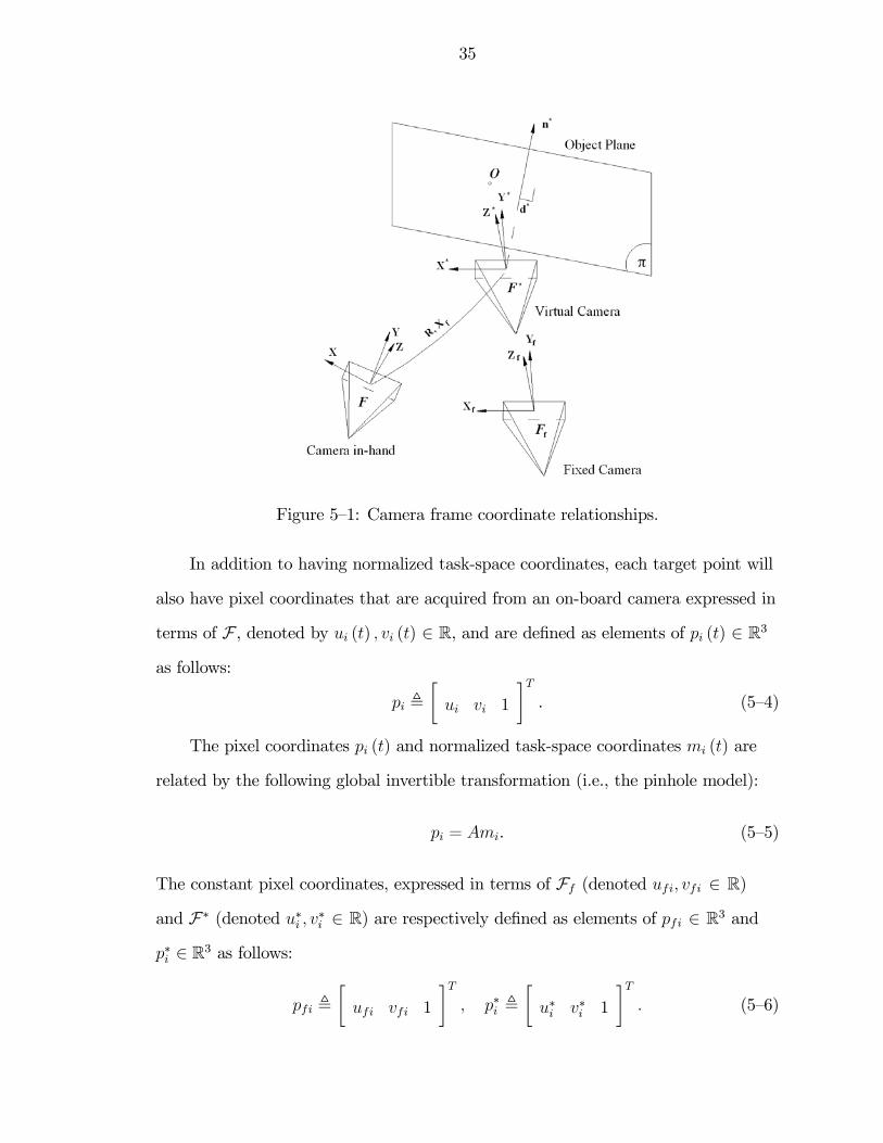
5—1 Camera frame coordinate relationships. . . . . . . . . . . . . . . . . . . . 35

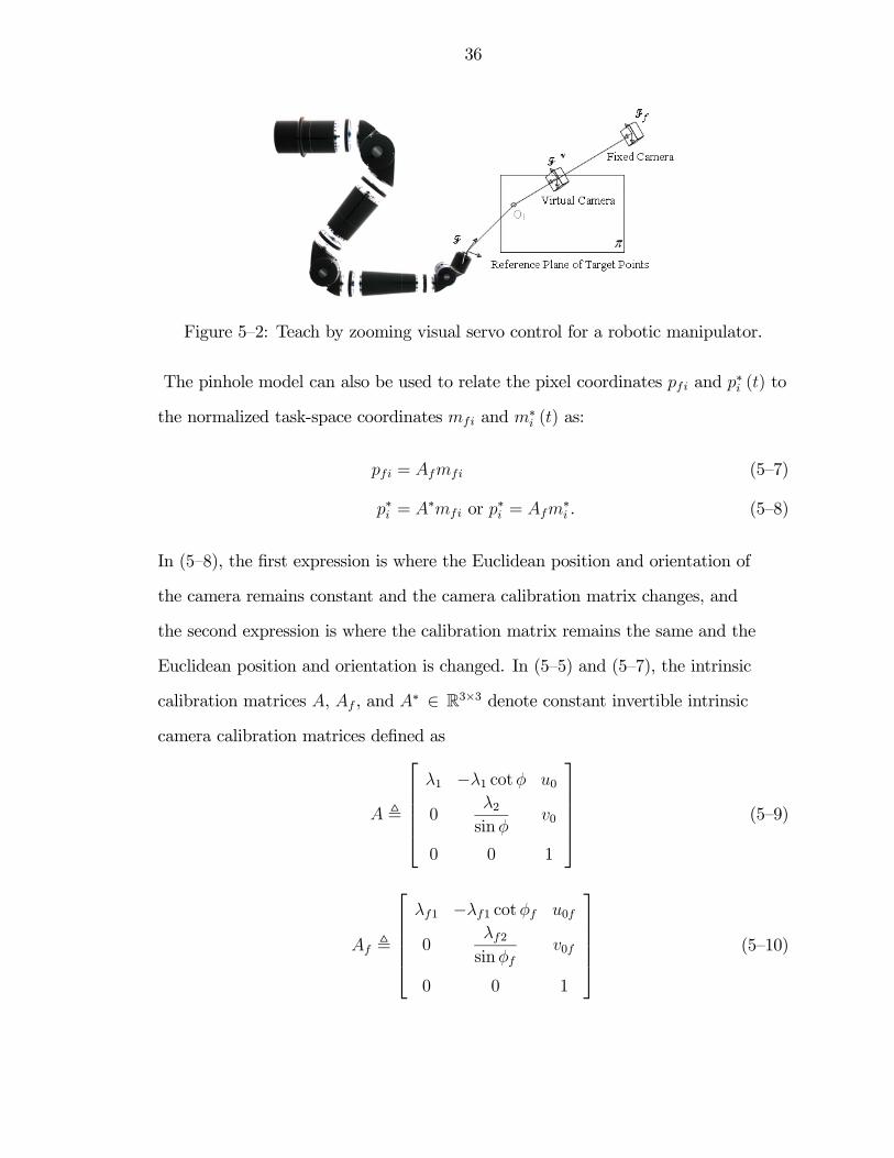
5—2 Teach by zooming visual servo control for a robotic manipulator. . . . . . 36

5—3 Overview of teach by zooming visual servo controller. . . . . . . . . . . . 42

5—4 Image from the fixed camera before zooming (subscript ‘f’) and afterzooming (superscript ‘*’). . . . . . . . . . . . . . . . . . . . . . . . . . . 52

5—5 Rotation Errors. . . . . . . . . . . . . . . . . . . . . . . . . . . . . . . . 52

5—6 Translation Errors. . . . . . . . . . . . . . . . . . . . . . . . . . . . . . . 53

5—7 Euclidean trajectory of the feature points viewed by the camera-in-handfrom the initial position and orientation (denoted by ‘+’) to the desiredposition and orientation Fd (denoted by ‘x’), where the virtual cameracoordinate system F∗ is denoted by ‘o’. . . . . . . . . . . . . . . . . . . 53

5—8 Angular control input velocity for the camera-in-hand. . . . . . . . . . . 54

5—9 Linear control input velocity for the camera-in-hand. . . . . . . . . . . . 54

5—10 Elimination of ineffectual feature points via. target identification. . . . . 55

5—11 Feature point matching between fixed camera and camera in-hand. . . . 56

6—1 Camera frame coordinate relationships. . . . . . . . . . . . . . . . . . . . 59

6—2 3D target reconstruction based visual servo control for a robotic manip-ulator. . . . . . . . . . . . . . . . . . . . . . . . . . . . . . . . . . . . . . 60

vii

6—3 Perspective projection geometry model for Euclidean depth identification. 62

6—4 Control architecture depicting rotation control. . . . . . . . . . . . . . . 64

6—5 Control architecture depicting translation control. . . . . . . . . . . . . . 65

6—6 Performance validation of 3D depth estimation. . . . . . . . . . . . . . . 69

6—7 Depth estimation error. . . . . . . . . . . . . . . . . . . . . . . . . . . . 70

6—8 Performance validation for repeatability test. . . . . . . . . . . . . . . . . 70

6—9 3D robot task-space depicting repeatability results. . . . . . . . . . . . . 72

6—10 Repeatability in xy-plane for the 3D target reconstruction based visualservo controller. . . . . . . . . . . . . . . . . . . . . . . . . . . . . . . . . 73

6—11 Repeatability in xz-plane for the 3D target reconstruction based visualservo controller. . . . . . . . . . . . . . . . . . . . . . . . . . . . . . . . . 73

6—12 Performance validation for experiment II. . . . . . . . . . . . . . . . . . . 74

6—13 Performance validation for experiment III. . . . . . . . . . . . . . . . . . 75

viii

LIST OF TABLES

Table page

5—1 List of variables for teach by zooming visual servo control. . . . . . . . . 34

6—1 List of variables for 3D target reconstruction based visual servo control. . 59

6—2 Performance validation for 3D depth estimation method. . . . . . . . . . 69

6—3 Actual Euclidean target position expressed in a fixed camera frame androbot base frame. . . . . . . . . . . . . . . . . . . . . . . . . . . . . . . . 71

6—4 Estimated Euclidean target position expressed in a fixed camera frame,robot base frame, and robot tool frame. . . . . . . . . . . . . . . . . . . 71

6—5 Initial robot end-effector position expressed in robot base frame . . . . . 71

6—6 Final robot end-effector position expressed in robot base frame. . . . . . 72

6—7 Actual Euclidean target position expressed in a fixed camera frame androbot base frame. . . . . . . . . . . . . . . . . . . . . . . . . . . . . . . . 74

6—8 Initial and final robot end-effector position expressed in robot base frame. 75

6—9 Actual Euclidean target position expressed in a fixed camera frame androbot base frame and initial and final robot end-effector position expressedin robot base frame. . . . . . . . . . . . . . . . . . . . . . . . . . . . . . 76

ix

Abstract of Thesis Presented to the Graduate Schoolof the University of Florida in Partial Fulfillment of theRequirements for the Degree of Master of Science

VISION-BASED CONTROL FOR AUTONOMOUS ROBOTIC CITRUSHARVESTING

By

Siddhartha Satish Mehta

May 2007

Chair: Thomas F. BurksMajor: Agricultural and Biological Engineering

Vision-based autonomous robotic citrus harvesting requires target detection

and interpretation of 3-dimensional (3D) Euclidean position of the target through

2D images. The typical visual servoing problem is constructed as a “teach by

showing” (TBS) problem. The teach by showing approach is formulated as the

desire to position/orient a camera based on a reference image obtained by a priori

positioning the same camera in the desired location. A new strategy is required for

the unstructured citrus harvesting application where the camera can not be a priori

positioned to the desired position/orientation. Therefore a “teach by zooming”

approach is proposed whereby the objective is to position/orient a camera based

on a reference image obtained by another camera. For example, a fixed camera

providing a global view of the tree canopy can zoom in on an object and record

a desired image for a camera in-hand. A controller is designed to regulate the

image features acquired by a camera in-hand to the corresponding image feature

coordinates in the desired image acquired by the fixed camera. The controller

is developed based on the assumption that parametric uncertainty exists in the

camera calibration since precise values for these parameters are difficult to obtain

x

in practice. Simulation results demonstrate the performance of the developed

controller.

However, the non-identical feature point matching between the two cameras

limits the application of teach by zooming visual servo controller to the artificial

targets, where the feature point information is available a priori. Therefore, a new

visual servo control strategy based on 3D reconstruction of the target from the

2D images is developed. The 3D reconstruction is achieved by using the statistical

data, viz. the mean diameter of the citrus fruit, along with the target image size

and the camera focal length to generate the 3D depth information. A controller

is developed to regulate the robot end-effector to the 3D Euclidean coordinates

corresponding to the centroid of the target fruit. The autonomous robotic citrus

harvesting facility provides a rapid prototyping testbed for evaluating such visual

servo control techniques. Experimental validation of the 3D target reconstruction-

based visual servo control technique demonstrates the feasibility of the controller

for an unstructured citrus harvesting application.

xi

CHAPTER 1INTRODUCTION

Mechanization of harvesting of fruits is highly desirable in developing countries

due to decrease in seasonal labor availability and increasing economic pressures.

The mechanized fruit harvesting technology has limitations to soft fruit harvesting

because of the occurrence of excessive damage to the harvest. Mechanical harvest-

ing systems are based on the principle of shaking or knocking the fruit out of the

tree. There are two basic types namely trunk shaker and canopy shake. The trunk

shaker based systems attempt to remove the fruit from the tree by simply shaking

or vibrating the tree trunk and allowing the induced vibrations and oscillations

to cause the fruit to fall out of the tree. Canopy shaker systems consist of nylon

rods that rotate and shake foliage. These nylon rods allow for better shaking of

the canopy than the trunk shakers alone. However, there are various problems

associated with these strictly mechanical harvester systems. Typically citrus has

strong attachment between the tree branch and the fruit, hence it may require

large amount of shaking for harvesting the fruit which may cause damage to the

tree, such as bark removal and broken branches. Moreover, due to mechanical

shaking system and conveyor belt collection systems, mechanical harvester systems

can cause fruit quality deterioration thus making mechanical harvesting systems

typically suitable for juice fruit quality. Since there is still a large percentage of

citrus that is sold as fresh market fruit and which cannot be damaged in any way.

An alternative to mechanical harvesting systems, yielding superior fruit quality, is

the use of automated robotic harvesting systems.

Characteristics of the automated fruit harvesting robot: (a) Able to locate

the fruits on the tree in three dimensions (3D) (b) able to approach and reach for

1

2

the fruit (c) able to detach the fruit according to a predetermined criterion, and

transfer it to a suitable container and (d) to be propelled in the orchard with ease

of maneuverability, from tree to tree and row to row, while negotiating various

terrains and topographies. In addition, a desirable capability is the versatility to

handle a variety of fruit crops with minimal changes in the general configuration

[30].

All these operations should be performed within the following constrains;

Picking rate faster than, or equal to, manual picking (by a group of workers),

Fruit quality equal to or superior to that obtained with manual picking, and

Economically justifiable.

Robots perform well in structured environment, where the Euclidean position

and orientation of target and obstacles is known. But, in presence of unstructured

urban/non-urban environments the difficulty is faced of determining the three

dimensional Euclidean position and orientation of the target and path planning

for obstacle avoidance. The traditional industrial application of robotics involve

structured environment, but robotics field is spreading to reach non-traditional

application areas such as medical robots and agricultural pre-harvesting and post-

harvesting. These non-traditional applications represent working of a robot in an

unstructured environment.

Several autonomous/semi-autonomous techniques have been proposed for

the target detection and range identification in unstructured environments. Ceres

et al. [3] developed an-aided fruit harvesting strategy where the operator drives

the robotic harvester and performs the detection of fruits by means of a laser

rangefinder; the computer performs the precise location of the fruits, computes

adequate picking sequences and controls the motion of manipulator joints. The

infrared laser range-finder used is based on the principle of phase shift between

emitted and reflected amplitude modulated laser signal. Since, the process of

3

detection and the localization of the fruit is directed by a human operator, this

approach heavily depends on human interface in the harvesting. D’Esnon et al. [14]

proposed an apple harvesting prototype robot— MAGALI, implementing a spherical

manipulator, mounted on a hydraulically actuated self guided vehicle, servoed by

a camera set mounted at the base rotation joint. When the camera detects a fruit,

the manipulator arm is orientated along the line of sight onto the coordinates of the

target and is moved forward till it reaches the fruit, which is sensed by a proximity

sensor. However, the use of proximity sensor could result in damaging the harvest

or manipulator. Moreover, the vision system implemented requires the camera to

be elevated along the tree to scan the tree from bottom to top. Rabatel et al. [29]

initiated a French Spanish EUREKA project named CITRUS, which was largely

based on the development of French robotic harvester MAGALI. The CITRUS

robotic system used a principle for robot arm motion: once the fruit is detected,

the straight line between the camera optical center and the fruit can be used as

a trajectory for the picking device to reach the fruit, as this line is guaranteed to

be free of obstacles. The principle used here is the same as MAGALI, and thus

this approach also fails to determine the three dimensional (3-D) position of the

fruit in the Euclidean workspace. Bulanon et al. [2] developed the method for

determining 3-D location of the apples for robotic harvesting using camera in-hand

configuration. Bulanon et al. used the differential object size method and binocular

stereo vision method for 3-D position estimation. In differential size method, the

change in the object size as the camera moves towards the object was used to

compute the distance, whereas the binocular stereo vision method calculates the

distance of the object from the camera using two images from different viewpoints

on the triangular measurement principle. However, range identification accuracy

of these methods was not satisfactory for robotic guidance. In addition Bulanon

et al. considered laser ranging technique for accurate range identification of the

4

object. Murakami et al.[28] proposed a vision-based robotic cabbage harvester. The

robot consists of a three degrees of freedom (3-DOF) polar hydraulic manipulator

and a color CCD camera is used for machine vision. Murakami et al. suggested

the use of hydraulic manipulator since they have high power to weight ratio and

do not require high power supply to automate the system, which is justified for

the cabbage harvesting application. The image processing strategy is to recognize

the cabbage heads by processing the color image which is taken under unstable

lighting conditions in the field. The image processing uses neural network to

extract cabbage heads of the HIS transformed image. The location and diameter

of cabbage are estimated by correlation with the image template. Since cabbage

harvesting represents a 2-D visual servo control problem, it is possible to apply the

template matching technique for 3-D location estimation. But for applications like

citrus harvesting, which require 3-D visual servo control of robotic manipulator,

exact three dimensional Euclidean coordinates are to be determined. Hayashi et al.

studied the development of robotic harvesting system that performs recognition,

approach, and picking tasks for eggplants [19]. The robotic harvesting system

consists of a machine vision system, a manipulator unit, and an end-effector unit.

The articulated manipulator with 5-DOF with camera in-hand configuration

was selected for harvesting application. A fuzzy logic based visual servo control

techniques were adapted for manipulator guidance. The visual feedback fuzzy

control model was designed to determine the forward movement, vertical movement

and rotational angle of the manipulator based on the position of the detected fruit

in an image frame. When the area occupied by the fruit is more than 70% of the

total image, the servoing is stopped and eggplant is picked.

With recent advances in camera technology, computer vision, and control the-

ory, visual servo control systems exhibit significant promise to enable autonomous

systems with the ability to operate in unstructured environments. Although a

5

vision system can provide a unique sense of perception, several technical issues

have impacted the design of robust visual servo controllers. One of these issues

includes the camera configuration (pixel resolution versus field-of-view). For ex-

ample, for vision systems that utilize a camera in a fixed configuration (i.e., the

eye-to-hand configuration), the camera is typically mounted at a large enough

distance to ensure that the desired target objects will remain in the camera’s

view. Unfortunately, by mounting the camera in this configuration the task-space

area that corresponds to a pixel in the image-space can be quite large, resulting

in low resolution and noisy position measurements. Moreover, many applications

are ill-suited for the fixed camera configuration. For example, a robot may be

required to position the camera for close-up tasks (i.e., the camera-in-hand configu-

ration). For the camera-in-hand configuration, the camera is naturally close to the

workspace, providing for higher resolution measurements due to the fact that each

pixel represents a smaller task-space area; however, the field-of-view of the camera

is significantly reduced (i.e., an object may be located in the workspace but be out

of the camera’s view).

Several results have been recently developed to address the camera config-

uration issues by utilizing a cooperative camera strategy. The advantages of the

cooperative camera configuration are that the fixed camera can be mounted so

that the complete workspace is visible and the camera-in-hand provides a high

resolution, close-up view of an object (e.g., facilitating the potential for more

precise motion for robotic applications). Specifically, Flandin et al. [13] made the

first steps towards cooperatively utilizing global and local information obtained

from a fixed camera and a camera-in-hand, respectively; unfortunately, to prove the

stability results, the translation and rotation tasks of the controller were treated

separately (i.e., the coupling terms were ignored) and the cameras were considered

to be calibrated. Dixon et al. [6], [7] developed a new cooperative visual servoing

6

approach and experimentally demonstrated to use information from both an uncali-

brated fixed camera and an uncalibrated camera-in-hand to enable robust tracking

by the camera-in-hand of an object moving in the task-space with an unknown

trajectory. Unfortunately, a crucial assumption for this approach is that the camera

and the object motion be constrained to a plane so that the unknown depth from

the camera to the target remains constant. The approaches presented by Dixon

et al. [6], [7] and Flandin et al. [13] are in contrast to typical multi-camera ap-

proaches, that utilize a stereo-based configuration, since stereo-based approaches

typically do not simultaneously exploit local and global views of the robot and the

workspace.

Another issue that has impacted the development of visual servo systems is the

calibration of the camera. For example, to relate pixelized image-space information

to the task-space, exact knowledge of the camera calibration parameters is required,

and discrepancies in the calibration matrix result in an erroneous relationship.

Furthermore, an acquired image is a function of both the task-space position of

the camera and the intrinsic calibration parameters; hence, perfect knowledge

of the camera intrinsic parameters is also required to relate the relative position

of a camera through the respective images as it moves. For example, the typical

visual servoing problem is constructed as a “teach by showing” (TBS) problem

in which a camera is positioned at a desired location, a reference image is taken

(where the normalized task-space location is determined via the intrinsic calibration

parameters), the camera is moved away from the reference location, and then

repositioned at the reference location under visual servo control (which requires

that the calibration parameters did not change in order to reposition the camera to

the same task-space location given the same image). See [4], [20], [18], and [23] for

a further explanation and an overview of this problem formulation.

7

Unfortunately, for many practical applications it may not be possible to TBS

(i.e., it may not be possible to acquire the reference image by a priori positioning

the camera-in-hand to the desired location). As stated by Malis [23], the TBS

problem formulation is “camera-dependent” due to the hypothesis that the

camera intrinsic parameters during the teaching stage, must be equal to the

intrinsic parameters during servoing. Motivated by the desire to address this

problem, the basic idea of the pioneering development by Malis [22], [23] is to use

projective invariance to construct an error function that is invariant to the intrinsic

parameters, thus enabling the control objective to be met despite variations in the

intrinsic parameters. However, the fundamental idea for the problem formulation

is that an error system be constructed in an invariant space, and unfortunately, as

stated by Malis [22], [23] several control issues and a rigorous stability analysis of

the invariant space approach “have been left unresolved.”

Inspired by the previous issues and the development by Dixon et al. [7]

and Malis [22], [23], the presented work utilizes a cooperative camera scheme

to formulate a visual control problem that does not rely on the TBS paradigm.

Specifically, a calibrated camera-in-hand and a calibrated fixed camera are used

to facilitate a “teach by zooming” approach to formulate a control problem

with the objective to force the camera-in-hand to the exactly known Euclidean

position/orientation of a virtual camera defined by a zoomed image from a fixed

camera (i.e., the camera-in-hand does not need to be positioned in the desired

location a priori using this alternative approach). Since the intrinsic camera

calibration parameters may be difficult to exactly determine in practice, a second

control objective is defined as the desire to servo an uncalibrated camera-in-hand

so that the respective image corresponds to the zoomed image of an uncalibrated

fixed camera. For each case, the fixed camera provides a global view of a scene that

can be zoomed to provide a close-up view of the target. The reference image is

8

then used to servo the camera-in-hand. That is, the proposed “teach by zooming”

approach addresses the camera configuration issues by exploiting the wide scene

view of a fixed camera and the close-up view provided by the camera-in-hand.

CHAPTER 2FUNDAMENTALS OF FEATURE POINT TRACKING AND MULTI-VIEW

PHOTOGRAMMETRY

2.1 Introduction

This chapter provides introduction to feature point detection and tracking

techniques commonly used for vision-based control strategies along with multi-

view photogrammetry concepts to determine the relationship between various

camera frame coordinate systems. The chapter is organized in the following

manner. In Section 2.2, the image processing algorithm for real-time feature

detection and tracking is discussed. In Section 2.3, implementation of a multi-view

photogrammetry technique is illustrated, and concluding remarks are provided in

Section 2.4.

2.2 Image Processing

Many vision-based estimation and control strategies require real-time detection

and tracking of features. In order to eliminate the ineffectual feature points,

feature point detection and tracking is performed only on the target of interest.

Hence, color thresholding-based image segmentation methods are used for target

(i.e. citrus fruit) detection (see Appendix B.1). The most important segment of

the image processing algorithm (see Appendix B.2) is real-time identification of

features required for coordinated guidance, navigation and control in complex 3D

surroundings such as urban environments. The algorithm is developed in C/C++

using Visual Studio 6.0. Intel’s Open Source Computer Vision Library is utilized

for real-time implementation of most of the image processing functions. Also,

GNU Scientific Library (GSL) is used, which is a numerical library for C and C++

programming. GSL provides a wide range of mathematical routines for most of the

9

10

computation involved in the algorithms. The rest of this section describes feature

point detection and Kanade-Lucas-Tomasi (KLT) feature point tracking method.

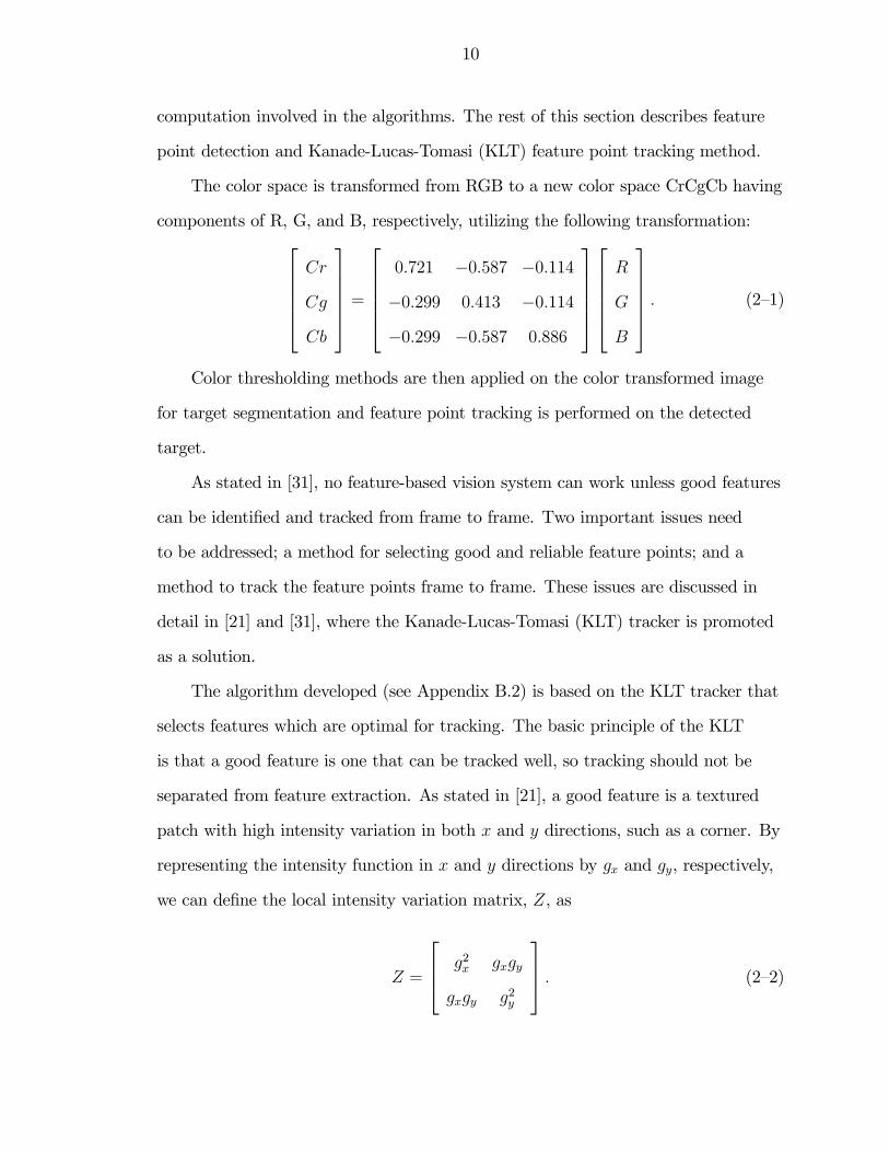
The color space is transformed from RGB to a new color space CrCgCb having

components of R, G, and B, respectively, utilizing the following transformation:⎡⎢⎢⎢⎢⎣Cr

Cg

Cb

⎤⎥⎥⎥⎥⎦ =⎡⎢⎢⎢⎢⎣0.721 −0.587 −0.114

−0.299 0.413 −0.114

−0.299 −0.587 0.886

⎤⎥⎥⎥⎥⎦⎡⎢⎢⎢⎢⎣

R

G

B

⎤⎥⎥⎥⎥⎦ . (2—1)

Color thresholding methods are then applied on the color transformed image

for target segmentation and feature point tracking is performed on the detected

target.

As stated in [31], no feature-based vision system can work unless good features

can be identified and tracked from frame to frame. Two important issues need

to be addressed; a method for selecting good and reliable feature points; and a

method to track the feature points frame to frame. These issues are discussed in

detail in [21] and [31], where the Kanade-Lucas-Tomasi (KLT) tracker is promoted

as a solution.

The algorithm developed (see Appendix B.2) is based on the KLT tracker that

selects features which are optimal for tracking. The basic principle of the KLT

is that a good feature is one that can be tracked well, so tracking should not be

separated from feature extraction. As stated in [21], a good feature is a textured

patch with high intensity variation in both x and y directions, such as a corner. By

representing the intensity function in x and y directions by gx and gy, respectively,

we can define the local intensity variation matrix, Z, as

Z =

⎡⎢⎣ g2x gxgy

gxgy g2y

⎤⎥⎦ . (2—2)

11

A patch defined by a 7 x 7 pixels window is accepted as a candidate feature if in

the center of the window both eigenvalues of Z, exceed a predefined threshold. Two

large eigenvalues can represent corners, salt and pepper textures, or any other pat-

tern that can be tracked reliably. Two small eigenvalues mean a roughly constant

intensity profile within a window. A large and a small eigenvalues correspond to a

unidirectional texture pattern. The intensity variations in a window are bounded

by the maximum allowable pixel value, so the greater eigenvalue cannot be arbi-

trarily large. In conclusion, if the two eigenvalues of Z are λ1 and λ2, we accept a

window if

min(λ1, λ2) > λ (2—3)

where λ is a predefined threshold.

As described in [31], feature point tracking is a standard task of computer

vision with numerous applications in navigation, motion understanding, surveil-

lance, scene monitoring, and video database management. In an image sequence,

moving objects are represented by their feature points detected prior to tracking

or during tracking. As the scene moves, the patterns of image intensities changes

in a complex way. Denoting images by I, these changes can be described as image

motion:

I(x, y, t+ τ) = I(x− ζ(x, y, t, τ), y − η(x, y, t, τ)). (2—4)

Thus a later image taken at time t + τ (where τ represents a small time interval)

can be obtained by moving every point in the current image, taken at time t, by a

suitable amount. The amount of motion δ = (ζ, η) is called the displacement of the

point at m = (x, y). The displacement vector δ is a function of image position m.

Tomasi in [31], states that pure translation is the best motion model for tracking

12

Figure 2—1: Moving camera looking at a reference plane.

because it exhibits reliability and accuracy in comparing features between the

reference and current image, hence

δ = d

where d is the translation of the feature’s window center between successive frames.

Thus, the knowledge of translation d allows reliable and optimal tracking of the

feature points windows.

In the algorithm developed for the teach by zooming visual servo control, the

method employed for tracking is based on the pyramidal implementation of the

KLT Tracker described in [1].

2.3 Multi-view Photogrammetry

The feature points data obtained during motion through the virtual environ-

ment is used to determine the relationship between the current and a constant

reference position as shown in Figure. 2—1. This relationship is obtained by deter-

mining the rotation and translation between corresponding feature points on the

current and reference image position. The rotation and translation components

13

relating corresponding points of the reference and current image is obtained by

first constructing the Euclidean homography matrix. Various techniques can then

be used (e.g., see [11], [32]) to decompose the Euclidean homography matrix into

rotational and translational components. Following section describes multiview

photogrammetry-based Euclidean reconstruction method to obtain unknown

rotation and translation vectors for camera motion.

Consider the orthogonal coordinate systems, denoted F and F∗ that are

depicted in Figure. 2—1. The coordinate system F is attached to a moving camera.

A reference plane π on the object is defined by four target points Oi ∀i = 1, 2, 3,

4 where the three dimensional (3D) coordinates of Oi expressed in terms of F and

F∗ are defined as elements of mi (t) and m∗i ∈ R3 and represented by

mi(t) ,∙xi(t) yi(t) zi(t)

¸T(2—5)

m∗i ,

∙x∗i y∗i z∗i

¸T. (2—6)

The Euclidean-space is projected onto the image-space, so the normalized coordi-

nates of the targets points mi (t) and m∗i are defined as

mi =mi

zi=

∙xizi

yizi

1

¸T(2—7)

m∗i =

m∗i

z∗i=

∙x∗iz∗i

y∗iz∗i

1

¸T(2—8)

under the standard assumption that zi (t) and z∗i > ε, where ε denotes an arbitrar-

ily small positive scalar constant.

Each target point has pixel coordinates that are acquired from the moving

camera, expressed in terms of F , denoted by ui (t) , vi (t) ∈ R, and are defined as

elements of pi (t) ∈ R3 as follows:

pi ,∙ui vi 1

¸T. (2—9)

14

The pixel coordinates of the target points at the reference position is expressed in

terms of F∗ (denoted by u∗i , v∗i ∈ R) and are defined as elements of p∗i ∈ R3 as

follows:

p∗i ,∙u∗i v∗i 1

¸T. (2—10)

The pixel coordinates pi (t) and p∗i are related by the following global invertible

transformation (i.e., the pinhole model) to the normalized task-space coordinates

mi (t) and m∗i , respectively:

pi = Ami (2—11)

p∗i = Am∗i

where A is the intrinsic camera calibration matrix.

The constant distance from the origin of F∗ to the object plane π along the

unit normal n∗ is denoted by d∗ ∈ R and is defined as

d∗ , n∗T m∗i . (2—12)

The coordinate frames F and F∗ depicted in Figure. 2—1 are attached to the

camera and denote the actual and reference locations of the camera. From the

geometry between the coordinate frames, m∗i can be related to mi(t) as follows

mi = xf +Rm∗i . (2—13)

In (2—13), R (t) ∈ SO(3) denotes the rotation between F and F∗, and xf (t) ∈ R3

denotes the translation vector from F to F∗ expressed in the coordinate frame F .

By utilizing (2—7), (2—8), and (2—12), the expressions in (2—13) can be written as

follows

mi = αi

¡R+ xhn

∗T¢| {z }m∗i .

H

(2—14)

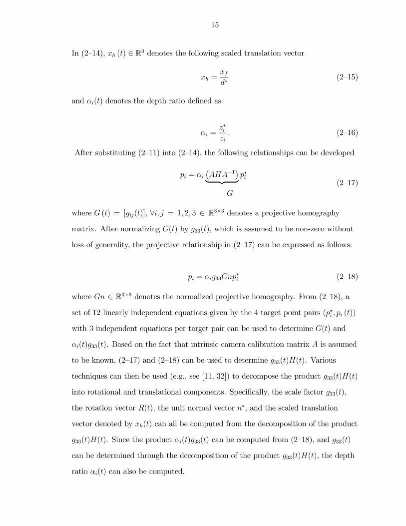
15

In (2—14), xh (t) ∈ R3 denotes the following scaled translation vector

xh =xfd∗

(2—15)

and αi(t) denotes the depth ratio defined as

αi =z∗izi. (2—16)

After substituting (2—11) into (2—14), the following relationships can be developed

pi = αi

¡AHA−1

¢| {z } p∗iG

(2—17)

where G (t) = [gij(t)], ∀i, j = 1, 2, 3 ∈ R3×3 denotes a projective homography

matrix. After normalizing G(t) by g33(t), which is assumed to be non-zero without

loss of generality, the projective relationship in (2—17) can be expressed as follows:

pi = αig33Gnp∗i (2—18)

where Gn ∈ R3×3 denotes the normalized projective homography. From (2—18), a

set of 12 linearly independent equations given by the 4 target point pairs (p∗i , pi (t))

with 3 independent equations per target pair can be used to determine G(t) and

αi(t)g33(t). Based on the fact that intrinsic camera calibration matrix A is assumed

to be known, (2—17) and (2—18) can be used to determine g33(t)H(t). Various

techniques can then be used (e.g., see [11, 32]) to decompose the product g33(t)H(t)

into rotational and translational components. Specifically, the scale factor g33(t),

the rotation vector R(t), the unit normal vector n∗, and the scaled translation

vector denoted by xh(t) can all be computed from the decomposition of the product

g33(t)H(t). Since the product αi(t)g33(t) can be computed from (2—18), and g33(t)

can be determined through the decomposition of the product g33(t)H(t), the depth

ratio αi(t) can also be computed.

16

2.4 Conclusion

In this chapter, we discussed techniques for real-time identification and

tracking of features required for teach by zooming visual servo control method.

The development included description of feature point tracking algorithms utilizing

Kanade-Lucas-Tomas tracker along with color thresholding-based image processing

methods and multi-view photogrammetry techniques are realized to relate various

coordinate frames.

CHAPTER 3OBJECTIVES

As described in Chapter 1, automated robotic citrus harvesting yields superior

fruit quality over the mechanical harvesting systems, which is highly desirable for

fresh fruit market. Characteristics of the automated fruit harvesting robot: (a)

Able to locate the fruits on the tree in three dimensions (3D) (b) able to approach

and reach for the fruit (c) able to detach the fruit according to a predetermined

criterion, and transfer it to a suitable container and (d) to be propelled in the

orchard with ease of maneuverability, from tree to tree and row to row, while

negotiating various terrains and topographies. The objective of the presented

work is to accomplish characteristics (a) and (b) of the automated fruit harvesting

system mentioned above. Color thresholding-based technique is realized for target

fruit identification, whereas multi-camera visual servo control techniques are

developed for 3D target position estimation and robot motion control.

With recent advances in camera technology, computer vision, and control the-

ory, visual servo control systems exhibit significant promise to enable autonomous

systems with the ability to operate in unstructured environments. Robotic harvest-

ing is one of the applications of visual servo control system working in unstructured

environment. Typical visual servoing control objectives are formulated by the desire

to position/orient a camera using multi-sensor stereovision techniques or based on

a reference image obtained by a priory positioning the same camera in the desired

location (i.e., the “teach by showing” approach). The shortcoming of stereovision

based visual servo control technique is lack of the three dimensional Euclidean task

space reconstruction. Also, teach by showing visual servo control technique is not

17

18

feasible for applications where the camera can not be a priori positioned to the

desired position/orientation.

A new cooperative control strategy, “teach by zooming (TBZ)” visual servo

control is proposed where the objective is to position/orient a camera based

on a reference image obtained by another camera. For example, a fixed camera

providing a global view of an object can zoom in on an object and record a desired

image for the camera-in-hand.

A technical issue that has impacted the design of robust visual servo con-

trollers is the camera configuration (i.e. the pixel resolution versus field-of-view).

Teach by zooming visual servo control technique effectively identifying both the

configurations provides high resolution images obtained by camera-in-hand and

large field-of-view by fixed camera. Another issue associated with visual servo

control systems is the camera calibration. In order to relate pixelized image-space

information to the three dimensional task-space, exact knowledge of the camera

calibration parameters is required, and discrepancies in the calibration matrix

result in an erroneous relationship between target image-space coordinates and the

corresponding Euclidean coordinates. Therefore, the controller is developed based

on the assumption that parametric uncertainty exists in the camera calibration

since precise values for these parameters are difficult to obtain in practice.

Homography-based techniques are used to decouple the rotation and transla-

tion components between the current image taken by camera-in-hand and desired

reference image taken by a fixed camera. Since teach by zooming control objective

is formulated in terms of images acquired from different uncalibrated cameras, the

ability to construct a meaningful relationship between the estimated and actual

rotation matrix is problematic. To overcome this challenge, the control objective is

formulated in terms of the normalized Euclidean coordinates. Specifically, desired

normalized Euclidean coordinates are defined as a function of the mismatch in the

19

camera calibration. This is a physically motivated relationship, since an image

is a function of both the Euclidean coordinates and the camera calibration. By

utilizing, Lyapunov-based methods, a controller is designed to regulate the image

features acquired by the camera-in-hand to the corresponding image feature coor-

dinates in the desired image acquired by the fixed camera. Since the estimates of

intrinsic calibration parameters are used in controller development the method is

robust to the camera calibration parameters. Also, proposed control scheme does

not rely on other sensors e.g. ultrasonic sensors, laser based, sensors, etc.

Another multi-camera visual servo control strategy, 3D target reconstruction

based visual servo control, has been proposed for target position estimation in the

Euclidean space. The technique utilizes statistical data along with camera intrinsic

parameters for 3D position estimation. Similar to teach by zooming visual servo

control, 3D target reconstruction based visual servo control technique effectively

utilizing both the configurations provides high resolution images obtained by

camera-in-hand and large field-of-view by fixed camera. The fixed camera providing

a global view of the target is used for target detection and image processing thus

optimizing the computation time, while using feedback from camera-in-hand during

visual servoing.

CHAPTER 4METHODS AND PROCEDURES

4.1 Introduction

This chapter provides an overview of the vision-based control techniques,

namely the teach by zooming visual servo controller and 3D target reconstruction

based visual servo controller, realized for autonomous citrus harvesting along with

the experimental testbed. The experimental facility provides a rapid prototyping

testbed for autonomous robotic guidance and control.

The hardware involved for the experimental testbed facility can be subdivided

into the following main components: (1) robotic manipulator; (2) end-effector; (3)

robot servo controller; (4) image processing workstation; and (5) network commu-

nication. The software developed for the autonomous robotic citrus harvesting is

based on image processing and computer vision methods, including feature point

tracking and multi-view photogrammetry techniques. An overview of vision-based

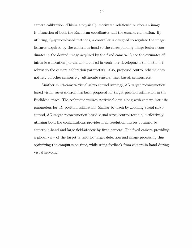
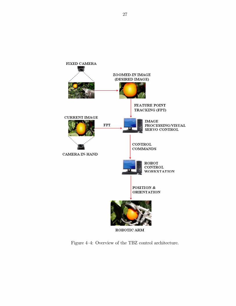
autonomous citrus harvesting method is illustrated in Figure. 4—1 and described as

follows:

1. Images of the citrus tree canopy are captured by a CCD camera and passed

to the image processing/visual servo control workstation through a USB analog to

digital converter and framegrabber.

2. Image processing and computer vision algorithms identify the target, i.e.

citrus fruit, from the image of a tree canopy. Feature points are identified and the

relationship between current and desired images is determined, in teach by zooming

visual servo control, to generate the control commands. In 3D target reconstruction

technique, the estimate for the Euclidean position of a target is determined to

provide the robot control workstation with control commands.

20

21

Figure 4—1: Overview of vision-based autonomous citrus harvesting.

3. Position and orientation commands are developed for robotic arm by the

robot control workstation utilizing low level controller.

4. Real-time network communication control is established between the image

processing workstation and robot control workstation.

The hardware setup of the experimental testbed facility is described in Section

4.2. Teach by zooming visual servo control method is described in Section 4.3,

while Section 4.4 illustrates the 3D target reconstruction based visual servo control

technique and concluding remarks are provided in Section 4.5.

4.2 Hardware Setup

The hardware for the experimental testbed for autonomous citrus harvesting

consists of the following five main components: (1) robotic manipulator; (2) end-

effector; (3) robot servo controller; (4) image processing workstation; and (5)

22

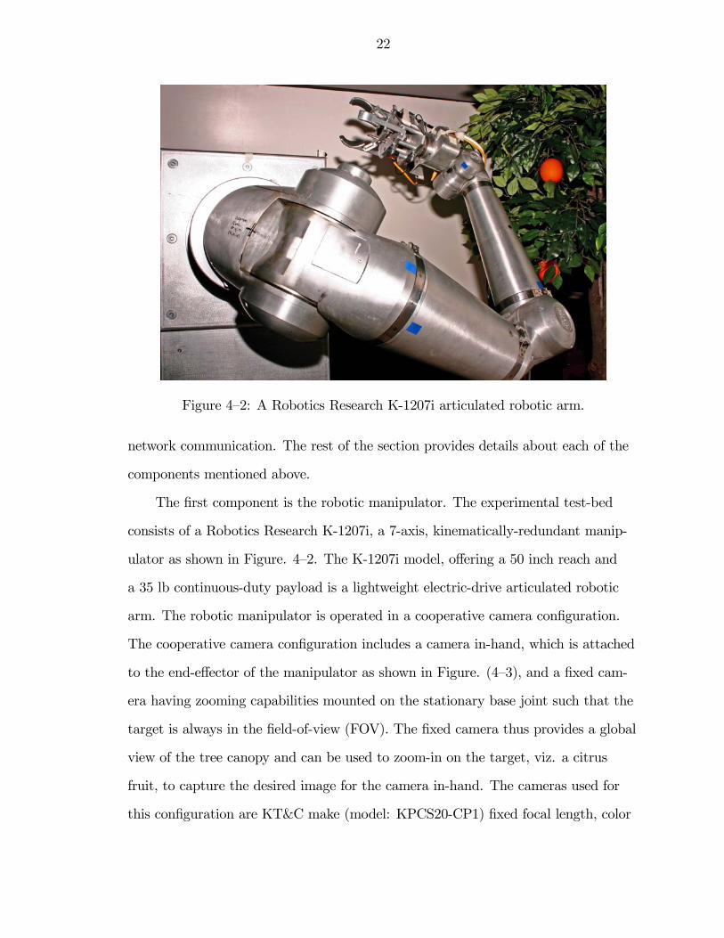
Figure 4—2: A Robotics Research K-1207i articulated robotic arm.

network communication. The rest of the section provides details about each of the

components mentioned above.

The first component is the robotic manipulator. The experimental test-bed

consists of a Robotics Research K-1207i, a 7-axis, kinematically-redundant manip-

ulator as shown in Figure. 4—2. The K-1207i model, offering a 50 inch reach and

a 35 lb continuous-duty payload is a lightweight electric-drive articulated robotic

arm. The robotic manipulator is operated in a cooperative camera configuration.

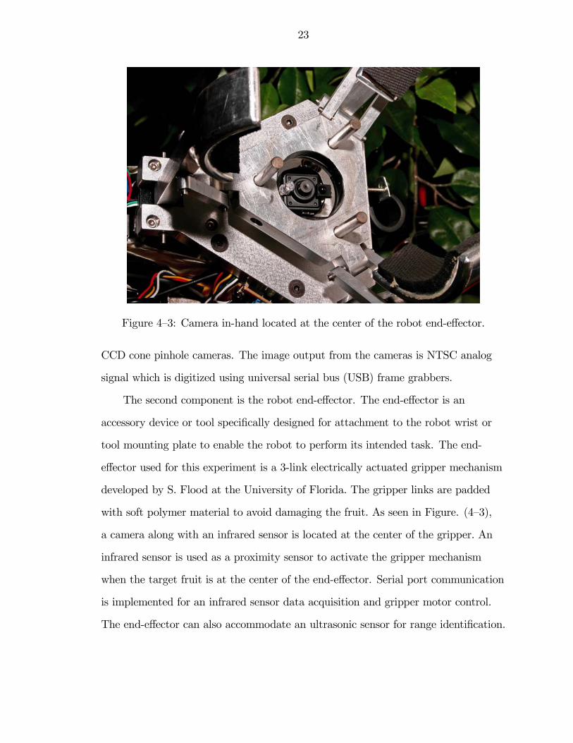
The cooperative camera configuration includes a camera in-hand, which is attached

to the end-effector of the manipulator as shown in Figure. (4—3), and a fixed cam-

era having zooming capabilities mounted on the stationary base joint such that the

target is always in the field-of-view (FOV). The fixed camera thus provides a global

view of the tree canopy and can be used to zoom-in on the target, viz. a citrus

fruit, to capture the desired image for the camera in-hand. The cameras used for

this configuration are KT&C make (model: KPCS20-CP1) fixed focal length, color

23

Figure 4—3: Camera in-hand located at the center of the robot end-effector.

CCD cone pinhole cameras. The image output from the cameras is NTSC analog

signal which is digitized using universal serial bus (USB) frame grabbers.

The second component is the robot end-effector. The end-effector is an

accessory device or tool specifically designed for attachment to the robot wrist or

tool mounting plate to enable the robot to perform its intended task. The end-

effector used for this experiment is a 3-link electrically actuated gripper mechanism

developed by S. Flood at the University of Florida. The gripper links are padded

with soft polymer material to avoid damaging the fruit. As seen in Figure. (4—3),

a camera along with an infrared sensor is located at the center of the gripper. An

infrared sensor is used as a proximity sensor to activate the gripper mechanism

when the target fruit is at the center of the end-effector. Serial port communication

is implemented for an infrared sensor data acquisition and gripper motor control.

The end-effector can also accommodate an ultrasonic sensor for range identification.

24

The third component of the autonomous citrus harvesting testbed is robot

servo control unit. The servo control unit provides a low level control of the robot

manipulator by generating the position/orientation commands for each joint.

Robotics Research R2 Control Software provides the low level robot control. The

robot controller consists of two primary components of operation; the INtime

real-time component (R2 RTC) and the NT client-server upper control level

component. The R2 RTC provides deterministic, hard real-time control with

typical loop times of 1 to 4 milliseconds. This component performs trajectory

planning, Cartesian compliance and impedance force control, forward kinematics,

and inverse kinematics. The controller can accept commands in the form of high

level Cartesian goal points down to low level servo commands of joint position,

torque or current. The robot servo control is performed on a Microsoft Windows

XP platform based IBM personal computer (PC) with 1.2 GHz Intel Pentium

Celeron processor and 512 MB random access memory (RAM).

The forth component is the image processing workstation, which is used for

image processing and vision-based control. Multi-camera visual servo control

technique described here consists of a fixed camera mounted on the stationary

base joint of the robot whereas a camera in-hand is attached to the robot end-

effector. The fixed camera provides a global view of the tree canopy and can

be used to capture the image for the target fruit. Microsoft DirectX and Intel

Open Computer Vision (OpenCV) libraries are used for image extraction and

interpretation, whereas Lucas-Kanade-Tomasi (KLT) based multi-resolution

feature point tracking algorithm, developed in Microsoft Visual C++ 6.0, tracks

the feature points detected in the previous stage in both the images. Multi-view

photogrammetry based method is used to compute the rotation and translation

between the camera in-hand frame and fixed camera frame utilizing the tracked

feature point information. A nonlinear Lyapunov-based controller, developed

25

in Chapter 5, is implemented to regulate the image features from the camera

in-hand to the desired image features acquired by the fixed camera. The image

processing and vision-based control are performed on a Microsoft Windows XP

platform based PC with 2.8 GHz Intel Pentium 4 processor and 512 MB RAM.

The fifth component is the network communication between the robot servo control

workstation and the image processing workstation. A deterministic and hard real-

time network communication control is established between these computers using

INtime software.

4.3 Teach by Zooming Visual Servo Control

Teach by zooming (TBZ) visual servo control approach is proposed for

applications where the camera cannot be a priori positioned to the desired

position/orientation to acquire a desired image before servo control. Specifically,

the TBZ control objective is formulated to position/orient an on-board camera

based on a reference image obtained by another camera. An overview of the

complete experimental testbed is illustrated in Figure. (4—4) and described in the

following steps:

1) Acquire the image of the target fruit for the fixed camera. The target fruit

can be selected manually or autonomously by implementing cost function based

image processing.

2) Digitally zoom-in the fixed camera on the target fruit to acquire the

desired image, which is passed to the image processing workstation. The amount

of magnification can be decided based on the size of a fruit in the image and the

image aspect ratio.

3) Run the feature point extraction and KLT-based multi-resolution feature

point tracking algorithm on the desired image for the fixed camera.

4) Orient the robot end-effector to capture the current image of the target by

the camera in-hand, which is passed to the image processing workstation.

26

5) Run the feature point extraction and tracking algorithm on the current

image for the camera in-hand.

6) Implement feature point matching to identify at least four identical feature

points between the current image and the desired image.

7) Compute the rotation and translation matrix between the current

and desired image frames utilizing the multi-view photogrammetry approach

(homography-based decomposition).

8) Rotation and translation matrix computed in step 6 can be used to compute

the desired rotation and translation velocity commands for the robot servo control.

9) The lower level controller generates the necessary position and orientation

commands for the robotic manipulator.

10) Approach the fruit and activate the gripper mechanism for harvesting a

fruit.

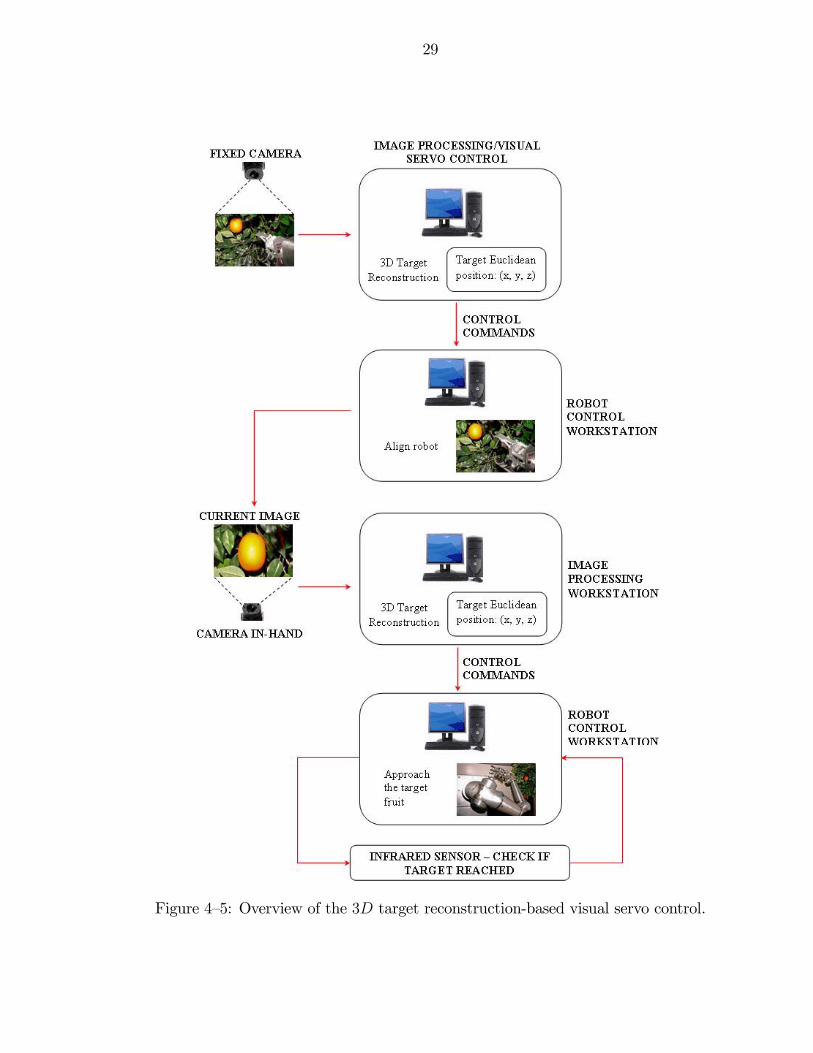
4.4 3D Target Reconstruction Based Visual Servo Control

The 3D Euclidean coordinates of the target fruit can be determined based on

the statistical mean diameter of the fruit as discussed later in Chapter 6. An end-

effector, and hence the camera in-hand, can be oriented such that the target fruit is

in the field-of-view of the camera in-hand. At this point, the Euclidean coordinates

of the target are again determined before approaching the fruit. An infrared sensor

is used as a proximity sensor for final approach towards the fruit and to activate

the gripper mechanism. An overview of the 3D target reconstruction based visual

servo control approach is illustrated in Figure. 4—5.

Following are the experimental steps or the harvesting sequence:

1) Acquire the image of the target fruit for the fixed camera. The target fruit

can be selected manually or autonomously by implementing cost function based

image processing.

27

Figure 4—4: Overview of the TBZ control architecture.

28

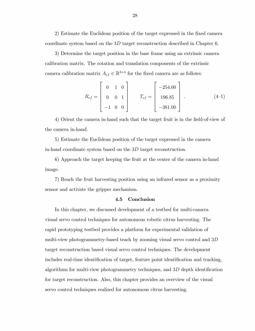
2) Estimate the Euclidean position of the target expressed in the fixed camera

coordinate system based on the 3D target reconstruction described in Chapter 6.

3) Determine the target position in the base frame using an extrinsic camera

calibration matrix. The rotation and translation components of the extrinsic

camera calibration matrix Aef ∈ R3×4 for the fixed camera are as follows:

Ref =

⎡⎢⎢⎢⎢⎣0 1 0

0 0 1

−1 0 0

⎤⎥⎥⎥⎥⎦ Tef =

⎡⎢⎢⎢⎢⎣−254.00

196.85

−381.00

⎤⎥⎥⎥⎥⎦ . (4—1)

4) Orient the camera in-hand such that the target fruit is in the field-of-view of

the camera in-hand.

5) Estimate the Euclidean position of the target expressed in the camera

in-hand coordinate system based on the 3D target reconstruction.

6) Approach the target keeping the fruit at the center of the camera in-hand

image.

7) Reach the fruit harvesting position using an infrared sensor as a proximity

sensor and activate the gripper mechanism.

4.5 Conclusion

In this chapter, we discussed development of a testbed for multi-camera

visual servo control techniques for autonomous robotic citrus harvesting. The

rapid prototyping testbed provides a platform for experimental validation of

multi-view photogrammetry-based teach by zooming visual servo control and 3D

target reconstruction based visual servo control techniques. The development

includes real-time identification of target, feature point identification and tracking,

algorithms for multi-view photogrammetry techniques, and 3D depth identification

for target reconstruction. Also, this chapter provides an overview of the visual

servo control techniques realized for autonomous citrus harvesting.

29

Figure 4—5: Overview of the 3D target reconstruction-based visual servo control.

CHAPTER 5TEACH BY ZOOMING VISUAL SERVO CONTROL FOR AN UNCALIBRATED

CAMERA SYSTEM

The teach by showing approach is formulated as the desire to position/orient

a camera based on a reference image obtained by a priori positioning the same

camera in the desired location. A new strategy is required for applications where

the camera can not be a priori positioned to the desired position/orientation. In

this chapter, a “teach by zooming” approach is presented where the objective is to

position/orient a camera based on a reference image obtained by another camera.

For example, a fixed camera providing a global view of an object can zoom-in on an

object and record a desired image for the camera in-hand (e.g. a camera mounted

on the fixed base joint providing a goal image for an image-guided autonomous

robotic arm). A controller is designed to regulate the image features acquired by

a camera in-hand to the corresponding image feature coordinates in the desired

image acquired by the fixed camera. The controller is developed based on the

assumption that parametric uncertainty exists in the camera calibration since

precise values for these parameters are difficult to obtain in practice. Simulation

results demonstrate the performance of the developed controller.

5.1 Introduction

Recent advances in visual servo control have been motivated by the desire to

make vehicular/robotic systems more autonomous. One problem with designing

robust visual servo control systems is to compensate for possible uncertainty in the

calibration of the camera. For example, exact knowledge of the camera calibration

parameters is required to relate pixelized image-space information to the task-

space. The inevitable discrepancies in the calibration matrix result in an erroneous

30

31

relationship between the image-space and task-space. Furthermore, an acquired

image is a function of both the task-space position of the camera and the intrinsic

calibration parameters; hence, perfect knowledge of the intrinsic camera parameters

is also required to relate the relative position of a camera through the respective

images as it moves. For example, the typical visual servoing problem is constructed

as a teach by showing (TBS) problem, in which a camera is positioned at a

desired location, a reference image is acquired (where the normalized task-space

coordinates are determined via the intrinsic calibration parameters), the camera

is moved away from the reference location, and then the camera is repositioned

at the reference location by means of visual servo control (which requires that the

calibration parameters did not change in order to reposition the camera to the

same task-space location given the same image). See [4], [20], [18], and [23] for a

further explanation and an overview of the TBS problem formulation.

For many practical applications it may not be possible to TBS (i.e., it may not

be possible to acquire the reference image by a priori positioning a camera in-hand

to the desired location). As stated by Malis [23], the TBS problem formulation

is camera-dependent due to the assumption that the intrinsic camera parameters

must be the same during the teaching stage and during servo control. Malis [23],

[22] used projective invariance to construct an error function that is invariant of the

intrinsic parameters meeting the control objective despite variations in the intrinsic

parameters. However, the goal is to construct an error system in an invariant space,

and unfortunately, as stated by Malis [23], [22], several control issues and a rigorous

stability analysis of the invariant space approach has been left unresolved.

In this work, a teach by zooming (TBZ) approach [5] is proposed to posi-

tion/orient a camera based on a reference image obtained by another camera. For

example, a fixed camera providing a global view of the scene can be used to zoom

in on an object and record a desired image for an on-board camera. Applications

32

of the TBZ strategy could include navigating ground or air vehicles based on

desired images taken by other ground or air vehicles (e.g., a satellite captures a

“zoomed-in” desired image that is used to navigate a camera on-board a micro-air

vehicle (MAV), a camera can view an entire tree canopy and then zoom in to

acquire a desired image of a fruit product for high speed robotic harvesting). The

advantages of the TBZ formulation are that the fixed camera can be mounted

so that the complete task-space is visible, can selectively zoom in on objects of

interest, and can acquire a desired image that corresponds to a desired position

and orientation for a camera in-hand. The controller is designed to regulate the

image features acquired by an on-board camera to the corresponding image feature

coordinates in the desired image acquired by the fixed camera. The controller is

developed based on the assumption that parametric uncertainty exists in the cam-

era calibration since these parameters are difficult to precisely obtain in practice.

Since the TBZ control objective is formulated in terms of images acquired from

different uncalibrated cameras, the ability to construct a meaningful relationship

between the estimated and actual rotation matrix is problematic. To overcome this

challenge, the control objective is formulated in terms of the normalized Euclidean

coordinates. Specifically, desired normalized Euclidean coordinates are defined as a

function of the mismatch in the camera calibration. This is a physically motivated

relationship, since an image is a function of both the Euclidean coordinates and the

camera calibration.

This method builds on the previous efforts that have investigated the advan-

tages of multiple cameras working in a non-stereo pair. Specifically, Dixon et al.

[6], [7] developed a new cooperative visual servoing approach and experimentally

demonstrated that using information from both an uncalibrated fixed camera and

an uncalibrated on-board camera enables an on-board camera to track an object

moving in the task-space with an unknown trajectory. The development by Dixon

33

et al. [6], [7] is based on a crucial assumption that the camera and the object

motion is constrained to a plane so that the unknown distance from the camera to

the target remains constant . However, in contrast to development by Dixon et al.

[6], [7], an on-board camera motion in this work is not restricted to a plane. The

TBZ control objective is also formulated so that we can leverage previous control

development by Fang et al. [9] to achieve exponential regulation of an on-board

camera despite uncertainty in the calibration parameters.

Simulation results are provided to illustrate the performance of the developed

controller.

5.2 Model Development

Consider the orthogonal coordinate systems, denoted F , Ff , and F∗ that are

depicted in Figure. 5—1 and Figure. 5—2. The coordinate system F is attached to

an on-board camera (e.g., a camera held by a robot end-effector, a camera mounted

on a vehicle). The coordinate system Ff is attached to a fixed camera that has an

adjustable focal length to zoom in on an object. An image is defined by both the

camera calibration parameters and the Euclidean position of the camera; therefore,

the feature points of an object determined from an image acquired from the fixed

camera after zooming in on the object can be expressed in terms of Ff in one

of two ways: a different calibration matrix can be used due to the change in the

focal length, or the calibration matrix can be held constant and the Euclidean

position of the camera is changed to a virtual camera position and orientation.

The position and orientation of the virtual camera is described by the coordinate

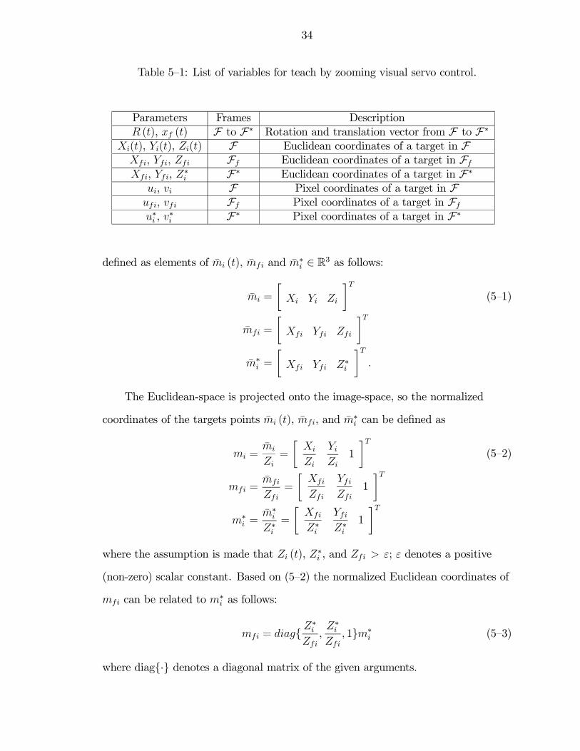
system F∗. Table 5-1 shows the parameters expressed in various coordinate frames.

A reference plane π is defined by four target points Oi ∀i = 1, 2, 3, 4 where the

three dimensional (3D) coordinates of Oi expressed in terms of F , Ff , and F∗ are

34

Table 5—1: List of variables for teach by zooming visual servo control.

Parameters Frames DescriptionR (t), xf (t) F to F∗ Rotation and translation vector from F to F∗

Xi(t), Yi(t), Zi(t) F Euclidean coordinates of a target in FXfi, Yfi, Zfi Ff Euclidean coordinates of a target in Ff

Xfi, Yfi, Z∗i F∗ Euclidean coordinates of a target in F∗ui, vi F Pixel coordinates of a target in Fufi, vfi Ff Pixel coordinates of a target in Ff

u∗i , v∗i F∗ Pixel coordinates of a target in F∗

defined as elements of mi (t), mfi and m∗i ∈ R3 as follows:

mi =

∙Xi Yi Zi

¸T(5—1)

mfi =

∙Xfi Yfi Zfi

¸Tm∗

i =

∙Xfi Yfi Z∗i

¸T.

The Euclidean-space is projected onto the image-space, so the normalized

coordinates of the targets points mi (t), mfi, and m∗i can be defined as

mi =mi

Zi=

∙Xi

Zi

YiZi

1

¸T(5—2)

mfi =mfi

Zfi=

∙Xfi

Zfi

YfiZfi

1

¸Tm∗

i =m∗

i

Z∗i=

∙Xfi

Z∗i

YfiZ∗i

1

¸Twhere the assumption is made that Zi (t), Z∗i , and Zfi > ε; ε denotes a positive

(non-zero) scalar constant. Based on (5—2) the normalized Euclidean coordinates of

mfi can be related to m∗i as follows:

mfi = diag{ Z∗i

Zfi,Z∗iZfi

, 1}m∗i (5—3)

where diag{·} denotes a diagonal matrix of the given arguments.

35

Figure 5—1: Camera frame coordinate relationships.

In addition to having normalized task-space coordinates, each target point will

also have pixel coordinates that are acquired from an on-board camera expressed in

terms of F , denoted by ui (t) , vi (t) ∈ R, and are defined as elements of pi (t) ∈ R3

as follows:

pi ,∙ui vi 1

¸T. (5—4)

The pixel coordinates pi (t) and normalized task-space coordinates mi (t) are

related by the following global invertible transformation (i.e., the pinhole model):

pi = Ami. (5—5)

The constant pixel coordinates, expressed in terms of Ff (denoted ufi, vfi ∈ R)

and F∗ (denoted u∗i , v∗i ∈ R) are respectively defined as elements of pfi ∈ R3 and

p∗i ∈ R3 as follows:

pfi ,∙ufi vfi 1

¸T, p∗i ,

∙u∗i v∗i 1

¸T. (5—6)

36

Figure 5—2: Teach by zooming visual servo control for a robotic manipulator.

The pinhole model can also be used to relate the pixel coordinates pfi and p∗i (t) to

the normalized task-space coordinates mfi and m∗i (t) as:

pfi = Afmfi (5—7)

p∗i = A∗mfi or p∗i = Afm∗i . (5—8)

In (5—8), the first expression is where the Euclidean position and orientation of

the camera remains constant and the camera calibration matrix changes, and

the second expression is where the calibration matrix remains the same and the

Euclidean position and orientation is changed. In (5—5) and (5—7), the intrinsic

calibration matrices A, Af , and A∗ ∈ R3×3 denote constant invertible intrinsic

camera calibration matrices defined as

A ,

⎡⎢⎢⎢⎢⎣λ1 −λ1 cotφ u0

0λ2sinφ

v0

0 0 1

⎤⎥⎥⎥⎥⎦ (5—9)

Af ,

⎡⎢⎢⎢⎢⎣λf1 −λf1 cotφf u0f

0λf2sinφf

v0f

0 0 1

⎤⎥⎥⎥⎥⎦ (5—10)

37

A∗ ,

⎡⎢⎢⎢⎢⎣λ∗1 −λ∗1 cotφf u0f

0λ∗2sinφf

v0f

0 0 1

⎤⎥⎥⎥⎥⎦ . (5—11)

In (5—9), (5—10), and (5—11), u0, v0 ∈ R and u0f , v0f ∈ R are the pixel coordinates

of the principal point of an on-board camera and fixed camera, respectively.

Constants λ1, λf1, λ∗1,λ2, λf2, λ∗2 ∈ R represent the product of the camera scaling

factors and focal length, and φ, φf ∈ R are the skew angles between the camera

axes for an on-board camera and fixed camera, respectively.

Since the intrinsic calibration matrix of a camera is difficult to accurately

obtain, the development is based on the assumption that the intrinsic calibration

matrices are unknown. Since Af is unknown, the normalized Euclidean coordinates

mfi cannot be determined from pfi using equation (5—7). Since mfi cannot be

determined, then the intrinsic calibration matrix A∗ cannot be computed from (5—

7). For the TBZ formulation, p∗i defines the desired image-space coordinates. Since

the normalized Euclidean coordinates m∗i are unknown, the control objective is

defined in terms of servoing an on-board camera so that the images correspond. If

the image from an on-board camera and the zoomed image from the fixed camera

correspond, then the following expression can be developed from (5—5) and (5—8):

mi = mdi , A−1Afm∗i (5—12)

where mdi ∈ R3 denotes the normalized Euclidean coordinates of the object

feature points expressed in Fd, where Fd is a coordinate system attached to an

on-board camera when the image taken from an on-board camera corresponds to

the image acquired from the fixed camera after zooming in on the object. Hence,

the control objective for the uncalibrated TBZ problem can be formulated as the

desire to force mi(t) to mdi. Given that mi(t), m∗i , and mdi are unknown, the

38

estimates mi (t) , m∗i , and mdi ∈ R3 are defined to facilitate the subsequent control

development [25]

mi = A−1pi = Ami (5—13)

m∗i = A−1f p∗i = Afm

∗i (5—14)

mdi = A−1p∗i = Amdi (5—15)

where A, Af ∈ R3×3 are constant, best-guess estimates of the intrinsic camera

calibration matrices and Af , respectively. The calibration error matrices A,

Af ∈ R3×3 are defined as

A , A−1A =

⎡⎢⎢⎢⎢⎣A11 A12 A13

0 A22 A23

0 0 1

⎤⎥⎥⎥⎥⎦ (5—16)

Af , A−1f Af =

⎡⎢⎢⎢⎢⎣Af11 Af12 Af13

0 Af22 Af23

0 0 1

⎤⎥⎥⎥⎥⎦ . (5—17)

For a standard TBS visual servo control problem where the calibration of the

camera does not change between the teaching phase and the servo phase, A = Af ;

hence, the coordinate systems Fd and F∗ are equivalent.

5.3 Homography Development

From Figure. 5—1 the following relationship can be developed

mi = Rm∗i + xf (5—18)

where R(t) ∈ R3×3 and xf(t) ∈ R3 denote the rotation and translation, respectively,

between F and F∗. By utilizing (5—1) and (5—2), the expression in (5—18) can be

39

expressed as follows

mi =

µZ∗iZi

¶| {z }

³R+ xhn

∗T´

| {z }m∗i (5—19)

αi H

where xh(t) , xf (t)

d∗ ∈ R3 and d∗ ∈ R denotes an unknown constant distance from

F∗ to π along the unit normal n∗. The following relationship can be developed by

substituting (5—19) and (5—8) into (5—5) for mi(t) and m∗i , respectively:

pi = αiGp∗i (5—20)

where G ∈ R3×3 is the projective homography matrix defined as G(t) , AH(t)A−1f .

The expressions in (5—5) and (5—8) can be used to rewrite (5—20) as

mi = αiA−1GAfm

∗i . (5—21)

The following expression can be obtained by substituting (5—12) into (5—21)

mi = αiHdmdi (5—22)

where Hd(t) , A−1G(t)A denotes the Euclidean homography matrix that can be

expressed as

Hd = Rd + xhdnTd where xhd =

xfddd

. (5—23)

In (5—23), Rd(t) ∈ R3×3 and xfd(t) ∈ R3 denote the rotation and translation,

respectively, from F to Fd. The constant dd ∈ R in (5—23) denotes the distance

from Fd to π along the unit normal nd ∈ R3.

Since mi(t) and m∗i cannot be determined because the intrinsic camera

calibration matrices and Af are uncertain, the estimates mi(t) and mdi defined in

(5—13) and (5—14), respectively, can be utilized to obtain the following:

mi = αiHdmdi. (5—24)

40

In (5—24), Hd (t) ∈ R3×3 denotes the following estimated Euclidean homography

[25]:

Hd = AHdA−1. (5—25)

Since mi(t) and mdi can be determined from (5—13) and (5—15), a set of linear

equations can be developed to solve for Hd (t) (see [8] for additional details

regarding the set of linear equations). The expression in (5—25) can also be

expressed as follows [8]:

Hd = Rd + xhdnTd . (5—26)

In (5—26), the estimated rotation matrix, denoted Rd (t) ∈ R3×3, is related to Rd (t)

as follows:

Rd = ARdA−1 (5—27)

and xhd (t) ∈ R3, nTd ∈ R3 denote the estimate of xhd (t) and nd, respectively, and

are defined as:

xhd = γAxhd (5—28)

nd =1

γA−Tnd (5—29)

where γ ∈ R denotes the following positive constant

γ =°°°A−Tnd°°° . (5—30)

Although Hd(t) can be computed, standard techniques cannot be used

to decompose Hd (t) into the rotation and translation components in (5—26).

Specifically, from (5—27) Rd(t) is not a true rotation matrix, and hence, it is not

clear how standard decomposition algorithms (e.g., the Faugeras algorithm [12])

can be applied. To address this issue, additional information (e.g., at least four

vanishing points) can be used. For example, as the reference plane π approaches

infinity, the scaling term d∗ also approaches infinity, and xh(t) and xh(t) approach

41

zero. Hence, (5—26) can be used to conclude that Hd(t) = Rd(t) on the plane

at infinity, and the four vanishing point pairs can be used along with (5—24) to

determine Rd(t). Once Rd(t) has been determined, various techniques (e.g., see

[10, 32]) can be used along with the original four image point pairs to determine

xhd(t) and nd(t).

5.4 Control Objective

The control objective is to ensure that the position and orientation of the

camera coordinate frame F is regulated to Fd. Based on Section 5.3, the control

objective is achieved if

Rd(t)→ I3 (5—31)

and one target point is regulated to its desired location in the sense that

mi(t)→ mdi and Zi(t)→ Zdi (5—32)

where I3 ∈ R3×3 represents an identity matrix.

To control the position and orientation of F , a relationship is required to

relate the linear and angular camera velocities to the linear and angular velocities

of the vehicle/robot (i.e., the actual kinematic control inputs) that enables an

on-board camera motion. This relationship is dependent on the extrinsic calibration

parameters as follows [25]:⎡⎢⎣ vc

ωc

⎤⎥⎦ =⎡⎢⎣ Rr [tr]×Rr

0 Rr

⎤⎥⎦⎡⎢⎣ vr

ωr

⎤⎥⎦ (5—33)

where vc(t), ωc(t) ∈ R3 denote the linear and angular velocity of the camera, vr(t),

ωr(t) ∈ R3 denote the linear and angular velocity of the vehicle/robot, Rr ∈ R3×3

denotes the unknown constant rotation between an on-board camera and robot

end-effector frames, and [tr]x ∈ R3×3 is a skew symmetric form of tr ∈ R3, which

denotes the unknown constant translation vector between an on-board camera and

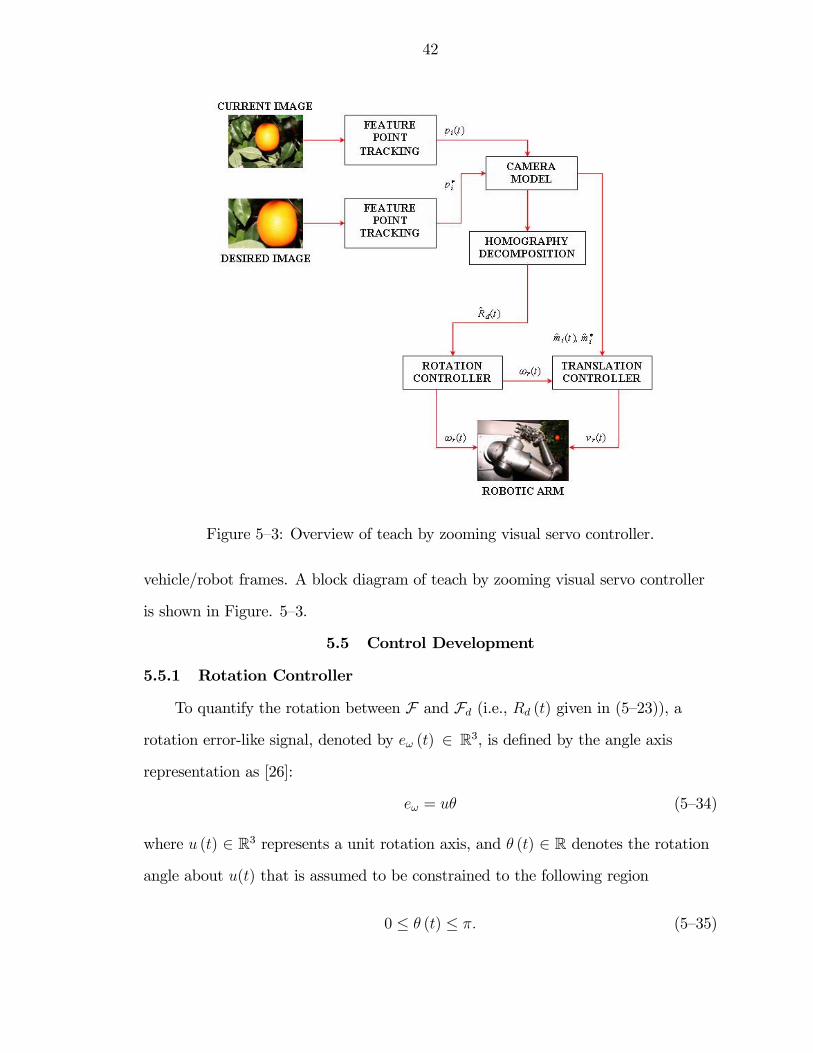
42

Figure 5—3: Overview of teach by zooming visual servo controller.

vehicle/robot frames. A block diagram of teach by zooming visual servo controller

is shown in Figure. 5—3.

5.5 Control Development

5.5.1 Rotation Controller

To quantify the rotation between F and Fd (i.e., Rd (t) given in (5—23)), a

rotation error-like signal, denoted by eω (t) ∈ R3, is defined by the angle axis

representation as [26]:

eω = uθ (5—34)

where u (t) ∈ R3 represents a unit rotation axis, and θ (t) ∈ R denotes the rotation

angle about u(t) that is assumed to be constrained to the following region

0 ≤ θ (t) ≤ π. (5—35)

43

The parameterization u (t) θ (t) is related to the rotation matrix Rd (t) as

Rd = I3 + sin θ [u]× + 2 sin2 θ

2[u]2× (5—36)

where [u]× denotes the 3 × 3 skew-symmetric matrix associated with u(t). The

open-loop error dynamics for eω(t) can be expressed as (Refer to Appendix A.1)

eω = LωRrωr (5—37)

where the Jacobian matrix Lω (t) ∈ R3×3 is defined as

Lω = I3 −θ

2[u]× +

⎛⎜⎜⎝1− sinc (θ)

sinc2µθ

2

¶⎞⎟⎟⎠ [u]2× . (5—38)

In equation (5—38) the sin c(θ) term is given by (5—39) as,

sin c(θ) =sin(θ)

θ. (5—39)

Since the rotation matrix Rd (t) and the rotation error eω (t) defined in (5—34)

are unmeasurable, an estimated rotation error eω(t) ∈ R3 is defined as

eω = uθ (5—40)

where u (t) ∈ R3, θ (t) ∈ R represent estimates of u (t) and θ (t), respectively. Since

Rd (t) is similar to Rd (t) (i.e., Rd (t) has the same trace and eigenvalues as Rd (t)),

the estimates u(t) and θ(t) can be related to u (t) and θ (t) as follows [25]:

θ = θ u = μAu (5—41)

where μ(t) ∈ R denotes the following unknown function

μ =1°°°Au°°° . (5—42)

44

The relationship in (5—41) allows eω(t) to be expressed in terms of the unmeasur-

able error eω(t) as

eω = μAeω. (5—43)

Given the open-loop rotation error dynamics in (5—37), the control input ωr(t)

is designed as

ωr = −λωRTr eω (5—44)

where λω ∈ R denotes a positive control gain, and Rr ∈ R3×3 denotes a constant

best-guess estimate of Rr. Substituting (5—43) into (5—44) and substituting the

resulting expression into (5—37) gives the following expression for the closed-loop

error dynamics [25]:

eω = −λωμLωRrAeω (5—45)

where the extrinsic rotation estimation error Rr ∈ R3×3 is defined as

Rr = RrRTr . (5—46)

The kinematic control input given in (5—44) ensures that eω (t) defined in

(5—34) is exponentially regulated in the sense that

keω(t)k ≤ keω(0)k exp(−λωμβ0t) (5—47)

provided the following inequality is satisfied:

xT³RrA

´x ≥ β0 kxk2 for ∀x ∈ R3 (5—48)

where

xT³RrA

´x = xT

³RrA

´Tx (5—49)

= xT

⎛⎜⎝RrA+³RrA

´T2

⎞⎟⎠x

45

for ∀x ∈ R3, and β0 ∈ R denotes the following minimum eigenvalue:

β0 = λmin

⎧⎪⎨⎪⎩RrA+

³RrA

´T2

⎫⎪⎬⎪⎭ . (5—50)

Proof: See [9].

5.5.2 Translation Controller

The difference between the actual and desired 3D Euclidean camera position,

denoted by the translation error signal ev (t) ∈ R3, is defined as

ev , me −mde (5—51)

where me (t) ∈ R3 denotes the extended coordinates of an image point on π

expressed in terms of F and is defined as1

me ,∙me1 (t) me2 (t) me3 (t)

¸T(5—52)

=

∙X1

Z1

Y1Z1

ln (Z1)

¸Tand mde ∈ R3 denotes the extended coordinates of the corresponding desired image

point on π in terms of Fd as

mde ,∙mde1 mde2 mde3

¸T(5—53)

=

∙Xd1

Z∗1

Yd1Z∗1

ln (Z∗1)

¸T

1 To develop the translation controller a single feature point can be utilized.Without loss of generality, the subsequent development will be based on the imagepoint O1, and hence, the subscript 1 will be utilized in lieu of i.

46

where ln (·) denotes the natural logarithm. Substituting (5—52) and (5—53) into

(5—51) yields

ev =

∙X1

Z1− Xd1

Z∗1

Y1Z1− Yd1

Z∗1ln

µZ1Z∗1

¶ ¸T(5—54)

where the ratio Z1Z∗1can be computed from (5—19) and the decomposition of the

estimated Euclidean homography in (5—24). Since m1(t) and md are unknown (since

the intrinsic calibration matrices are unknown), ev (t) is not measurable. Therefore,

the estimate of the translation error system given in (5—54) is defined as

ev ,∙me1 − mde1 me2 − mde2 ln

µZ1Z∗1

¶ ¸T(5—55)

where me1(t), me2(t), mde1, mde2 ∈ R denote estimates of me1(t), me2(t), mde1, mde2,

respectively.

To develop the closed-loop error system for ev (t), we take the time derivative

of (5—54) and then substitute (5—44) into the resulting expression for ωr (t) to

obtain (Refer to Appendix A.2)

ev = LvRrvr + λw¡Lv [tr]× + Lvω

¢Rreω (5—56)

where the Lv(t), Lvω(t) ∈ R3x3 are defined as

Lv ,1

Z1

⎡⎢⎢⎢⎢⎣−1 0 me1

0 −1 me2

0 0 −1

⎤⎥⎥⎥⎥⎦ (5—57)

Lvω ,

⎡⎢⎢⎢⎢⎣me1me2 −1−m2

e1 me2

1 +m2e2 −me1me2 −me1

−me2 me1 0

⎤⎥⎥⎥⎥⎦ . (5—58)

To facilitate the control development, the unknown depth Z1(t) in (5—57) can be

expressed as

Z1 =1

α1Z∗1 (5—59)

47

where α1 is given by the homography decomposition.

An estimate for Lv(t) can be designed as

Lv =1

Z1

⎡⎢⎢⎢⎢⎣−1 0 me1

0 −1 me2

0 0 −1

⎤⎥⎥⎥⎥⎦ , (5—60)

where me1(t), me2(t) were introduced in (5—55), and Z1 ∈ R is developed based on

(5—59) as

Z1 =1

α1Z∗1 . (5—61)

Based on the structure of the error system in (5—56) and subsequent stability

analysis, the following hybrid translation controller can be developed

vr(t) = −λvRTr L

Tv ev (5—62)

−³kn1Z

21 + kn2Z

21 kevk

2´RTr L

Tv ev

where RTr , ev(t), and Lv(t) are introduced in (5—44), (5—55), and (5—60), respec-

tively, kn1, kn2 ∈ R denote positive constant control gains, and Z1(t) is defined in

(5—61). In (5—62), λv(t) ∈ R denotes a positive gain function defined as

λv = kn0 +Z21

f (me1, me2)(5—63)

where kn0 ∈ R is a positive constant, and f (me1, me2) is a positive function of me1

and me2

The kinematic control input given in (5—62) ensures that the hybrid translation

error signal ev (t) defined in (5—54) is exponentially regulated in the sense that

kev(t)k ≤p2ζ0°°B−1°° exp(−ζ1

2t) (5—64)

provided (5—48) is satisfied, where B ∈ R3x3 is a constant invertible matrix, and ζ0,

ζ1 ∈ R denote positive constants.

48

Proof: See [9].

5.6 Simulation Results

5.6.1 Introduction

A numerical simulation is presented to illustrate the performance of the TBZ

controller given in (5—44) and (5—62). The simulation setup for teach by zooming

visual servo control consists of following three main components: (1) simulation

workstation, (2) simulation software, and (3) virtual camera. The rest of the

section provides details about each of the components mentioned above.

The first component is the simulation workstation. The vision-based control

simulation is performed on Microsoft Windows XP platform based IBM personal

computer (PC) with 3.06 GHz Intel Pentium 4 processor and 764 MB random

access memory (RAM).

The second component in the simulation is the software platform. MATLAB

(The MathWorks, Inc.) release 6.0 has been used for numerical simulation, along

with Simulink for interactive graphical environment. Simulink is a platform for

multidomain simulation and Model-Based Design for dynamic systems.

The third component in the simulation being the virtual camera. The intrinsic

camera calibration matrix is given in (5—68), whereas (5—65) and (5—66) state the

extrinsic camera calibration parameters. In the intrinsic camera calibration matrix

it is assumed that parametric uncertainty exists in the camera calibration since

these parameters are difficult to precisely obtain in practice.

The following section provides numerical results of the simulation.

5.6.2 Numerical Results

The intrinsic camera calibration matrix used for an on-board camera and the

fixed camera are given as follows: u0 = v0 = 120 [pixels] and u0f = v0f = 120

[pixels] denote the pixel coordinates of the principal point; λ1 = 122.5, λ2 = 122.5,

λf1 = 147, λf2 = 147, λ∗1 = 294, and λ∗2 = 294 denote the product of the

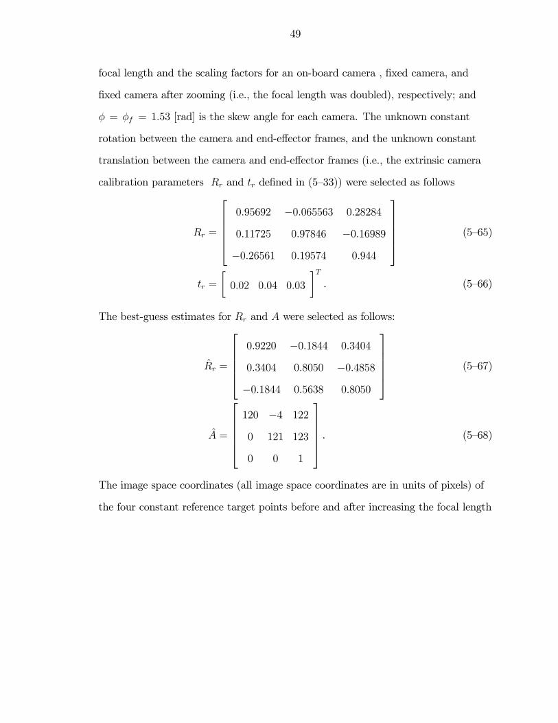
49

focal length and the scaling factors for an on-board camera , fixed camera, and

fixed camera after zooming (i.e., the focal length was doubled), respectively; and

φ = φf = 1.53 [rad] is the skew angle for each camera. The unknown constant

rotation between the camera and end-effector frames, and the unknown constant

translation between the camera and end-effector frames (i.e., the extrinsic camera

calibration parameters Rr and tr defined in (5—33)) were selected as follows

Rr =

⎡⎢⎢⎢⎢⎣0.95692 −0.065563 0.28284

0.11725 0.97846 −0.16989

−0.26561 0.19574 0.944

⎤⎥⎥⎥⎥⎦ (5—65)

tr =

∙0.02 0.04 0.03

¸T. (5—66)

The best-guess estimates for Rr and A were selected as follows:

Rr =

⎡⎢⎢⎢⎢⎣0.9220 −0.1844 0.3404

0.3404 0.8050 −0.4858

−0.1844 0.5638 0.8050

⎤⎥⎥⎥⎥⎦ (5—67)

A =

⎡⎢⎢⎢⎢⎣120 −4 122

0 121 123

0 0 1

⎤⎥⎥⎥⎥⎦ . (5—68)

The image space coordinates (all image space coordinates are in units of pixels) of

the four constant reference target points before and after increasing the focal length

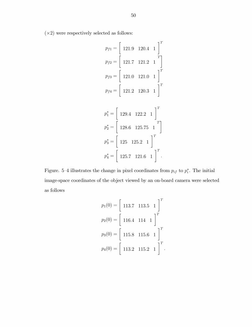
50

(×2) were respectively selected as follows:

pf1 =

∙121.9 120.4 1

¸Tpf2 =

∙121.7 121.2 1

T¸

pf3 =

∙121.0 121.0 1

¸Tpf4 =

∙121.2 120.3 1

¸T

p∗1 =

∙129.4 122.2 1

¸Tp∗2 =

∙128.6 125.75 1

T¸

p∗3 =

∙125 125.2 1

¸Tp∗4 =

∙125.7 121.6 1

¸T.

Figure. 5—4 illustrates the change in pixel coordinates from pif to p∗i . The initial

image-space coordinates of the object viewed by an on-board camera were selected

as follows

p1(0) =

∙113.7 113.5 1

¸Tp2(0) =

∙116.4 114 1

¸Tp3(0) =

∙115.8 115.6 1

¸Tp4(0) =

∙113.2 115.2 1

¸T.

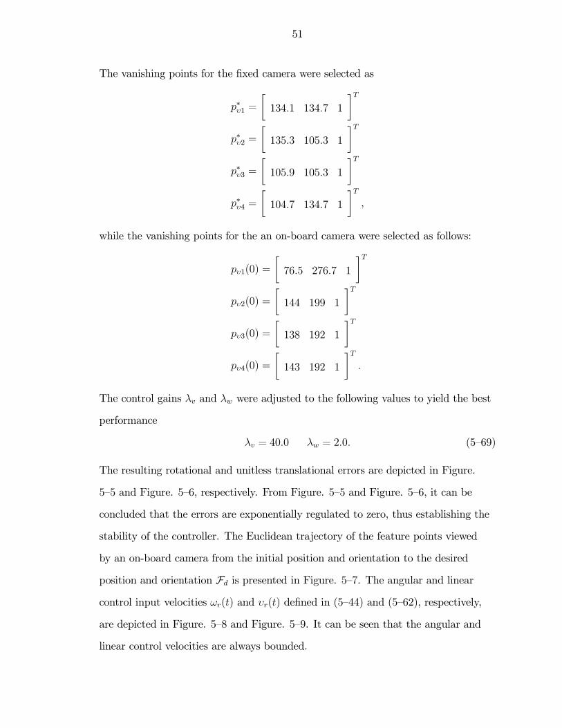
51

The vanishing points for the fixed camera were selected as

p∗υ1 =

∙134.1 134.7 1

¸Tp∗υ2 =

∙135.3 105.3 1

¸Tp∗υ3 =

∙105.9 105.3 1

¸Tp∗υ4 =

∙104.7 134.7 1

¸T,

while the vanishing points for the an on-board camera were selected as follows:

pυ1(0) =

∙76.5 276.7 1

¸Tpυ2(0) =

∙144 199 1

¸Tpυ3(0) =

∙138 192 1

¸Tpυ4(0) =

∙143 192 1

¸T.

The control gains λv and λw were adjusted to the following values to yield the best

performance

λv = 40.0 λw = 2.0. (5—69)

The resulting rotational and unitless translational errors are depicted in Figure.

5—5 and Figure. 5—6, respectively. From Figure. 5—5 and Figure. 5—6, it can be

concluded that the errors are exponentially regulated to zero, thus establishing the

stability of the controller. The Euclidean trajectory of the feature points viewed

by an on-board camera from the initial position and orientation to the desired

position and orientation Fd is presented in Figure. 5—7. The angular and linear

control input velocities ωr(t) and υr(t) defined in (5—44) and (5—62), respectively,

are depicted in Figure. 5—8 and Figure. 5—9. It can be seen that the angular and

linear control velocities are always bounded.

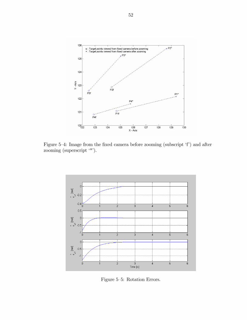
52

Figure 5—4: Image from the fixed camera before zooming (subscript ‘f’) and afterzooming (superscript ‘*’).

Figure 5—5: Rotation Errors.

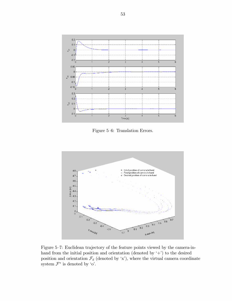
53

Figure 5—6: Translation Errors.

Figure 5—7: Euclidean trajectory of the feature points viewed by the camera-in-hand from the initial position and orientation (denoted by ‘+’) to the desiredposition and orientation Fd (denoted by ‘x’), where the virtual camera coordinatesystem F∗ is denoted by ‘o’.

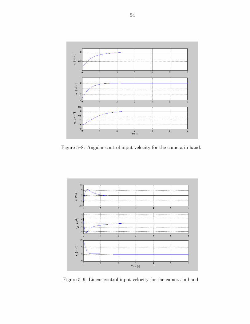
54

Figure 5—8: Angular control input velocity for the camera-in-hand.

Figure 5—9: Linear control input velocity for the camera-in-hand.

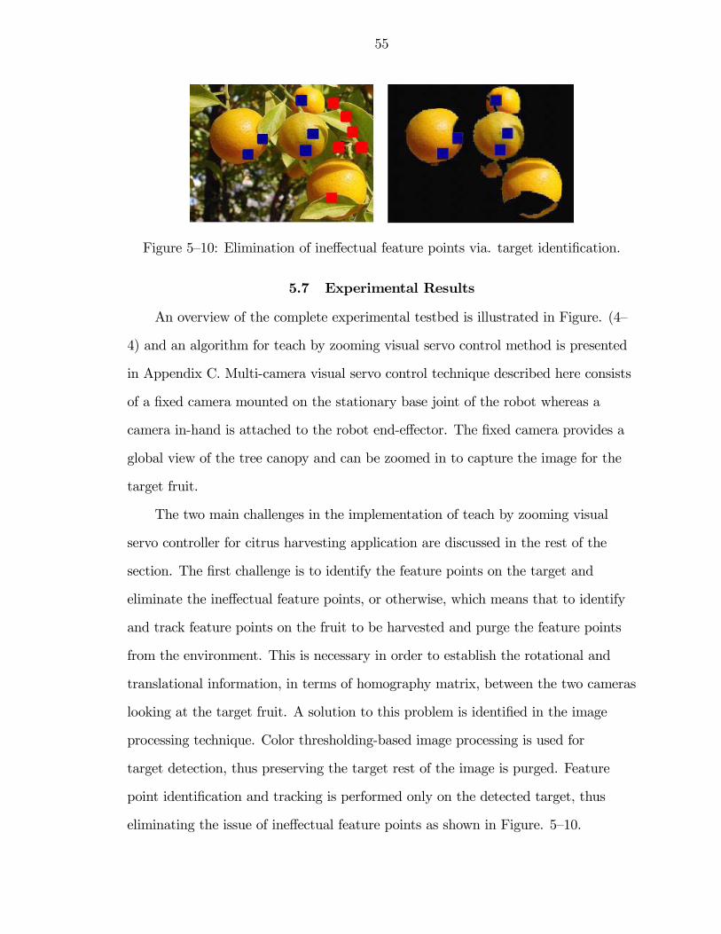
55

Figure 5—10: Elimination of ineffectual feature points via. target identification.

5.7 Experimental Results

An overview of the complete experimental testbed is illustrated in Figure. (4—

4) and an algorithm for teach by zooming visual servo control method is presented

in Appendix C. Multi-camera visual servo control technique described here consists

of a fixed camera mounted on the stationary base joint of the robot whereas a

camera in-hand is attached to the robot end-effector. The fixed camera provides a

global view of the tree canopy and can be zoomed in to capture the image for the

target fruit.

The two main challenges in the implementation of teach by zooming visual

servo controller for citrus harvesting application are discussed in the rest of the

section. The first challenge is to identify the feature points on the target and

eliminate the ineffectual feature points, or otherwise, which means that to identify

and track feature points on the fruit to be harvested and purge the feature points

from the environment. This is necessary in order to establish the rotational and

translational information, in terms of homography matrix, between the two cameras

looking at the target fruit. A solution to this problem is identified in the image

processing technique. Color thresholding-based image processing is used for

target detection, thus preserving the target rest of the image is purged. Feature

point identification and tracking is performed only on the detected target, thus

eliminating the issue of ineffectual feature points as shown in Figure. 5—10.

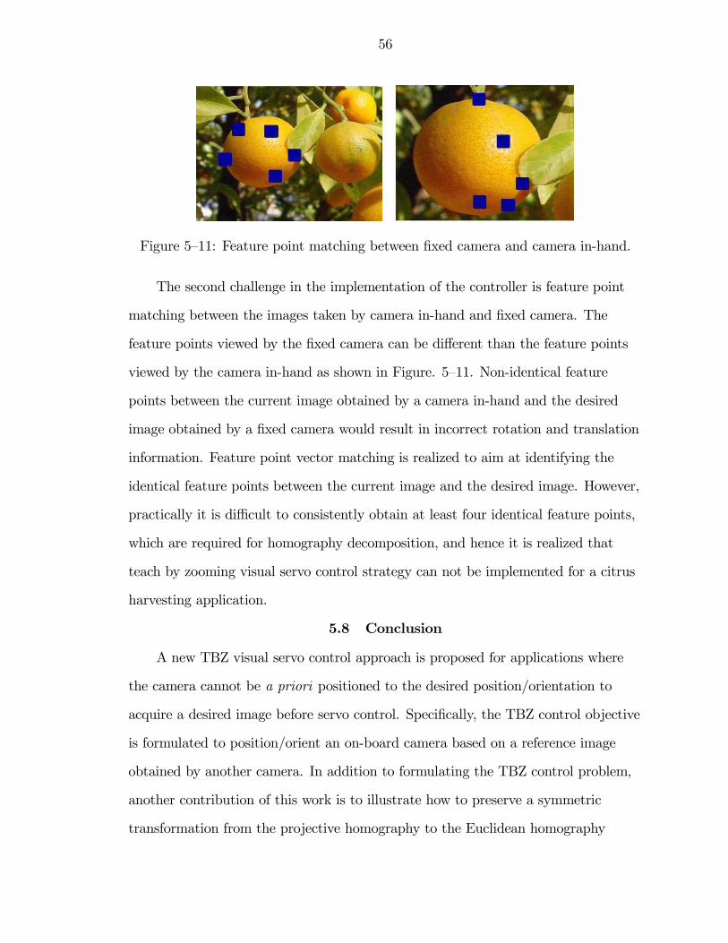
56

Figure 5—11: Feature point matching between fixed camera and camera in-hand.

The second challenge in the implementation of the controller is feature point

matching between the images taken by camera in-hand and fixed camera. The

feature points viewed by the fixed camera can be different than the feature points

viewed by the camera in-hand as shown in Figure. 5—11. Non-identical feature

points between the current image obtained by a camera in-hand and the desired

image obtained by a fixed camera would result in incorrect rotation and translation

information. Feature point vector matching is realized to aim at identifying the

identical feature points between the current image and the desired image. However,

practically it is difficult to consistently obtain at least four identical feature points,

which are required for homography decomposition, and hence it is realized that

teach by zooming visual servo control strategy can not be implemented for a citrus

harvesting application.

5.8 Conclusion

A new TBZ visual servo control approach is proposed for applications where

the camera cannot be a priori positioned to the desired position/orientation to

acquire a desired image before servo control. Specifically, the TBZ control objective

is formulated to position/orient an on-board camera based on a reference image

obtained by another camera. In addition to formulating the TBZ control problem,

another contribution of this work is to illustrate how to preserve a symmetric

transformation from the projective homography to the Euclidean homography

57

for problems when the corresponding images are taken from different cameras

with calibration uncertainty. To this end, a desired camera position/orientation

is defined where the images correspond, but the Euclidean position differs as a

function of the mismatch in the calibration of the cameras. Simulation results are

provided to illustrate the performance of the controller. Rotation and translation

errors are exponentially regulated to zero thus establishing the stability of the

controller, whereas the angular and linear control velocities are always bounded.

Applications of this strategy could include navigating ground or air vehicles, based

on desired images taken by other ground or air vehicles (e.g., a micro air vehicle

(MAV) captures a “zoomed in” desired image that is used to navigate an on-board

camera).

Practical limitation on the implementation of the teach by zooming visual

servo controller for the citrus harvesting application has been realized in the

fact that the feature points viewed by the fixed camera can be different than the

feature points viewed by the camera in-hand. Non-identical feature points between

the current image and the desired image would result in incorrect rotation and

translation information. Hence the teach by zooming visual servo controller can

be implemented where the feature point information is available a priori, i.e., this

controller is suitable for artificial targets.

CHAPTER 63D TARGET RECONSTRUCTION FOR VISION-BASED ROBOT CONTROL

The teach by zooming visual servo control strategy is devised to posi-

tion/orient a camera based on a reference image obtained by another camera.

As seen in Chapter 5, this strategy employs coordinated relationship between the

fixed camera and camera in-hand using the feature point matching technique.

However, feature point matching is not suitable for natural targets like citrus due

to non-identical feature point matching. Therefore, this chapter describes a visual

servo control strategy based on three dimensional (3D) reconstruction of the target

from a two dimensional (2D) image. The 3D target reconstruction is achieved by

using the statistical data, viz. the mean diameter and the standard deviation of the

citrus fruit diameter, along with the target image size and the camera focal length

to generate the 3D depth information. A controller is developed to regulate the

robot end-effector to the 3D Euclidean coordinates corresponding to the centroid of

the target fruit.

6.1 Model Development

Consider the orthogonal coordinate systems, denoted F , Ff , and F∗ that are

depicted in Figure. 6—1 and Figure. 6—2. The coordinate system F is attached to

an on-board camera (e.g., a camera held by a robot end-effector, a camera mounted

on a vehicle). The coordinate system Ff is attached to a fixed camera (e.g. a

camera mounted on a stationary base joint of a robot) and the coordinate system

F∗ is attached to a target fruit with fruit centroid being the coordinate system

origin. Table 6-1 shows the parameters expressed in various coordinate frames. The

origin of the coordinate system F∗ is denoted as i, where the three dimensional

(3D) coordinates of i expressed in terms of F and Ff are defined as elements of

58

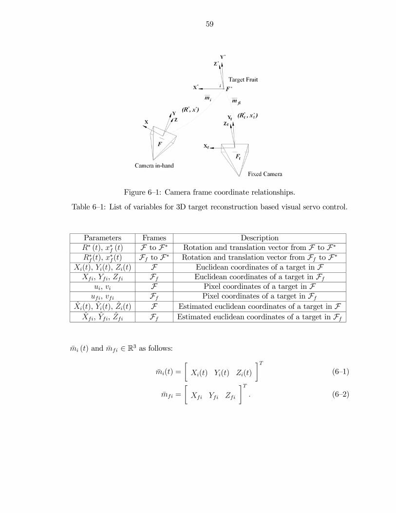
59

Figure 6—1: Camera frame coordinate relationships.

Table 6—1: List of variables for 3D target reconstruction based visual servo control.

Parameters Frames DescriptionR∗ (t), x∗f (t) F to F∗ Rotation and translation vector from F to F∗R∗f(t), x

∗f(t) Ff to F∗ Rotation and translation vector from Ff to F∗

Xi(t), Yi(t), Zi(t) F Euclidean coordinates of a target in FXfi, Yfi, Zfi Ff Euclidean coordinates of a target in Ff

ui, vi F Pixel coordinates of a target in Fufi, vfi Ff Pixel coordinates of a target in Ff

Xi(t), Yi(t), Zi(t) F Estimated euclidean coordinates of a target in FXfi, Yfi, Zfi Ff Estimated euclidean coordinates of a target in Ff

mi (t) and mfi ∈ R3 as follows:

mi(t) =

∙Xi(t) Yi(t) Zi(t)

¸T(6—1)

mfi =

∙Xfi Yfi Zfi

¸T. (6—2)

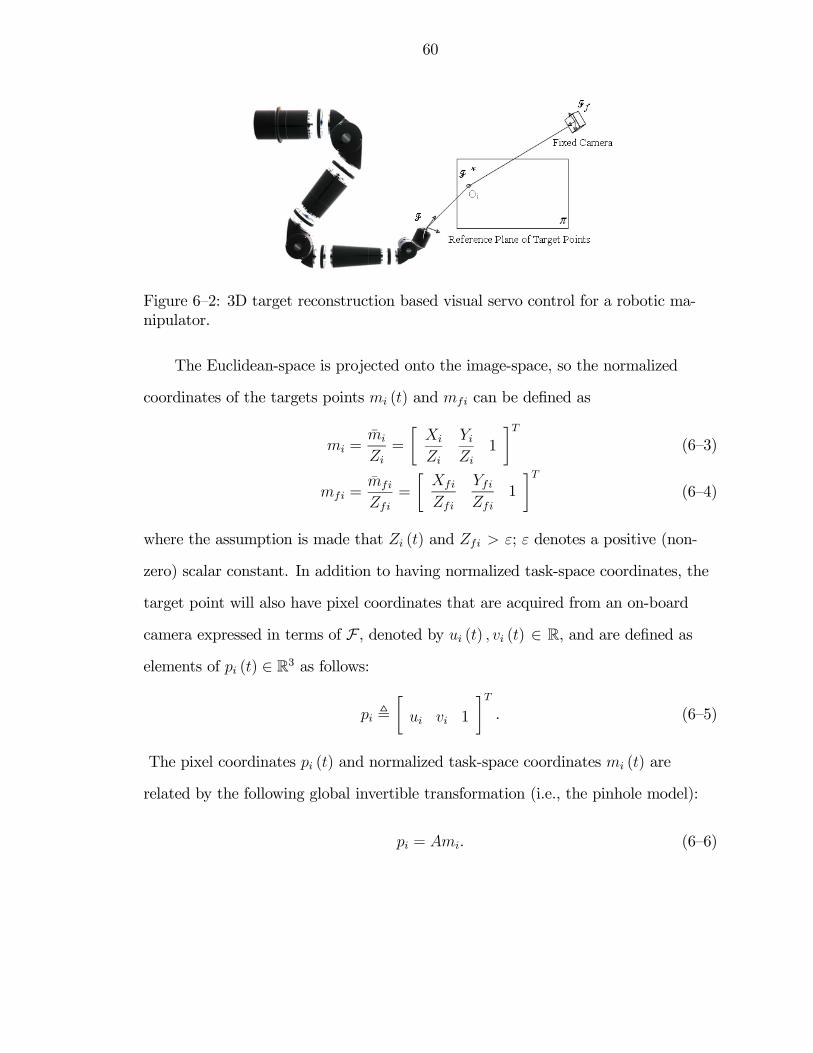
60

Figure 6—2: 3D target reconstruction based visual servo control for a robotic ma-nipulator.

The Euclidean-space is projected onto the image-space, so the normalized

coordinates of the targets points mi (t) and mfi can be defined as

mi =mi

Zi=

∙Xi

Zi

YiZi

1

¸T(6—3)

mfi =mfi

Zfi=

∙Xfi

Zfi

YfiZfi

1

¸T(6—4)

where the assumption is made that Zi (t) and Zfi > ε; ε denotes a positive (non-

zero) scalar constant. In addition to having normalized task-space coordinates, the

target point will also have pixel coordinates that are acquired from an on-board

camera expressed in terms of F , denoted by ui (t) , vi (t) ∈ R, and are defined as

elements of pi (t) ∈ R3 as follows:

pi ,∙ui vi 1

¸T. (6—5)

The pixel coordinates pi (t) and normalized task-space coordinates mi (t) are

related by the following global invertible transformation (i.e., the pinhole model):

pi = Ami. (6—6)

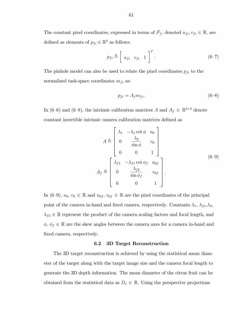
61

The constant pixel coordinates, expressed in terms of Ff , denoted ufi, vfi ∈ R, are

defined as elements of pfi ∈ R3 as follows:

pfi ,∙ufi vfi 1

¸T. (6—7)

The pinhole model can also be used to relate the pixel coordinates pfi to the

normalized task-space coordinates mfi as:

pfi = Afmfi. (6—8)

In (6—6) and (6—8), the intrinsic calibration matrices A and Af ∈ R3×3 denote

constant invertible intrinsic camera calibration matrices defined as

A ,

⎡⎢⎢⎢⎢⎣λ1 −λ1 cotφ u0

0λ2sinφ

v0

0 0 1

⎤⎥⎥⎥⎥⎦

Af ,

⎡⎢⎢⎢⎢⎣λf1 −λf1 cotφf u0f

0λf2sinφf

v0f

0 0 1

⎤⎥⎥⎥⎥⎦ .(6—9)

In (6—9), u0, v0 ∈ R and u0f , v0f ∈ R are the pixel coordinates of the principal

point of the camera in-hand and fixed camera, respectively. Constants λ1, λf1,λ2,

λf2 ∈ R represent the product of the camera scaling factors and focal length, and

φ, φf ∈ R are the skew angles between the camera axes for a camera in-hand and

fixed camera, respectively.

6.2 3D Target Reconstruction

The 3D target reconstruction is achieved by using the statistical mean diam-

eter of the target along with the target image size and the camera focal length to

generate the 3D depth information. The mean diameter of the citrus fruit can be

obtained from the statistical data as Do ∈ R. Using the perspective projections

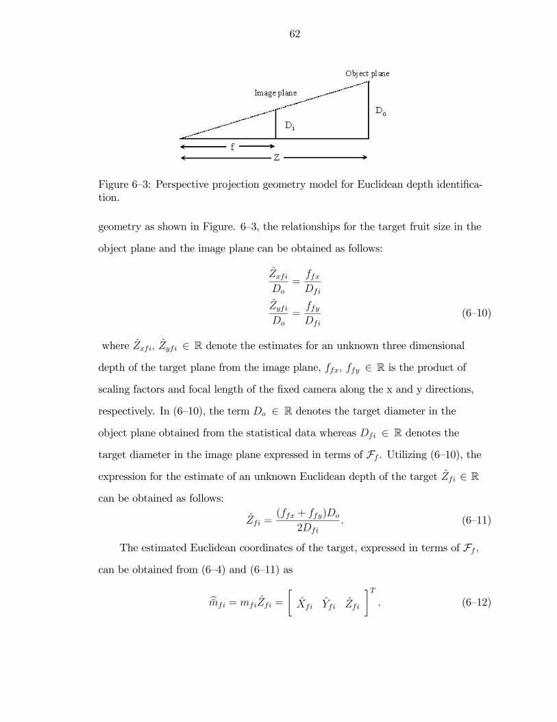
62

Figure 6—3: Perspective projection geometry model for Euclidean depth identifica-tion.

geometry as shown in Figure. 6—3, the relationships for the target fruit size in the

object plane and the image plane can be obtained as follows:

Zxfi

Do=

ffxDfi

Zyfi

Do=

ffyDfi

(6—10)

where Zxfi, Zyfi ∈ R denote the estimates for an unknown three dimensional

depth of the target plane from the image plane, ffx, ffy ∈ R is the product of

scaling factors and focal length of the fixed camera along the x and y directions,

respectively. In (6—10), the term Do ∈ R denotes the target diameter in the

object plane obtained from the statistical data whereas Dfi ∈ R denotes the

target diameter in the image plane expressed in terms of Ff . Utilizing (6—10), the

expression for the estimate of an unknown Euclidean depth of the target Zfi ∈ R

can be obtained as follows:

Zfi =(ffx + ffy)Do

2Dfi. (6—11)

The estimated Euclidean coordinates of the target, expressed in terms of Ff ,

can be obtained from (6—4) and (6—11) as

bmfi = mfiZfi =

∙Xfi Yfi Zfi

¸T. (6—12)

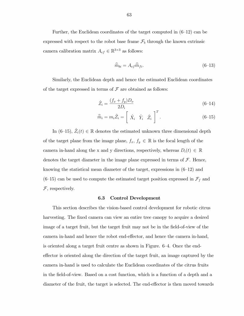
63

Further, the Euclidean coordinates of the target computed in (6—12) can be

expressed with respect to the robot base frame Fb through the known extrinsic

camera calibration matrix Aef ∈ R3×3 as follows:

bmbi = Aef bmfi. (6—13)

Similarly, the Euclidean depth and hence the estimated Euclidean coordinates

of the target expressed in terms of F are obtained as follows:

Zi =(fx + fy)Do

2Di(6—14)

bmi = miZi =

∙Xi Yi Zi

¸T. (6—15)

In (6—15), Zi(t) ∈ R denotes the estimated unknown three dimensional depth

of the target plane from the image plane, fx, fy ∈ R is the focal length of the

camera in-hand along the x and y directions, respectively, whereas Di(t) ∈ R

denotes the target diameter in the image plane expressed in terms of F . Hence,

knowing the statistical mean diameter of the target, expressions in (6—12) and

(6—15) can be used to compute the estimated target position expressed in Ff and

F , respectively.

6.3 Control Development

This section describes the vision-based control development for robotic citrus

harvesting. The fixed camera can view an entire tree canopy to acquire a desired

image of a target fruit, but the target fruit may not be in the field-of-view of the

camera in-hand and hence the robot end-effector, and hence the camera in-hand,

is oriented along a target fruit centre as shown in Figure. 6—4. Once the end-

effector is oriented along the direction of the target fruit, an image captured by the

camera in-hand is used to calculate the Euclidean coordinates of the citrus fruits

in the field-of-view. Based on a cost function, which is a function of a depth and a

diameter of the fruit, the target is selected. The end-effector is then moved towards

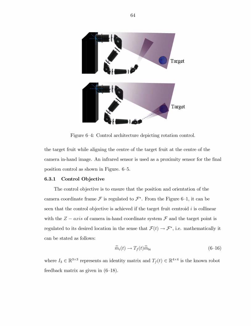
64

Figure 6—4: Control architecture depicting rotation control.

the target fruit while aligning the centre of the target fruit at the centre of the

camera in-hand image. An infrared sensor is used as a proximity sensor for the final

position control as shown in Figure. 6—5.

6.3.1 Control Objective

The control objective is to ensure that the position and orientation of the

camera coordinate frame F is regulated to F∗. From the Figure 6—1, it can be

seen that the control objective is achieved if the target fruit centroid i is collinear

with the Z − axis of camera in-hand coordinate system F and the target point is

regulated to its desired location in the sense that F(t)→ F∗, i.e. mathematically it

can be stated as follows: bmi(t)→ Tf(t) bmbi (6—16)

where I3 ∈ R3×3 represents an identity matrix and Tf(t) ∈ R4×4 is the known robot

feedback matrix as given in (6—18).

65

Figure 6—5: Control architecture depicting translation control.

6.3.2 Rotation Controller

The estimated target position expressed in the robot base frame Fb can be

stated in the camera in-hand coordinate frame F through the robot feedback

matrix Tf(t) as follows: ∙ bmi 1

¸T= Tf

∙ bmbi 1

¸T(6—17)

where the feedback matrix Tf(t) can be written in terms of the rotation and

translation vectors Rf(t) ∈ R3×3 and Pf(t) =

∙xf(t) yf(t) zf(t)

¸T∈ R3,

respectively, as:

Tf =

⎡⎢⎣ Rf Pf

0 1

⎤⎥⎦ . (6—18)

The objective of the rotation controller is to align the z-axis of the camera in-hand

frame F , i.e., the z-axis of the robot end-effector, along the target fruit centroid.

The rotation control objective can be achieved by rotating the robot end-effector

about the x-axis through an angle α(t) ∈ R and y-axis though an angle β(t) ∈ R.

66

The rotation angles α(t) and β(t) can be quantified as below

α = tan−1

ÃYi

Zi

!(6—19)

β = − tan−1ÃXi

Zi

!. (6—20)

Hence the rotation of the robot end-effector about x and y axis can be ex-

pressed in terms of rotation matrices Rx(t) ∈ R3×3 and Ry(t) ∈ R3×3, respectively,

as follows:

Rx =

⎡⎢⎢⎢⎢⎣1 0 0

0 cos(α) sin(α)

0 − sin(α) cos(α)

⎤⎥⎥⎥⎥⎦ Ry =

⎡⎢⎢⎢⎢⎣cos(β) 0 − sin(β)

0 1 0

sin(β) 0 cos(β)

⎤⎥⎥⎥⎥⎦ (6—21)

where α(t) and β(t) are defined in (6—19) and (6—20), respectively. Further, the

rotations Rx(t) and Ry(t) can be expressed in the robot base frame Fb as:

Rbx = RfRx Rby = RfRy. (6—22)

Rotation error signal eω(t) ∈ R3 can be quantified as the mismatch between

the robot feedback Rf(t) and the desired rotations calculated in (6—22) in terms of

rotation about x, y, z − axis of the robot base frame as follows:.

eω(t) =

∙α(t) β(t) γ(t)

¸T. (6—23)

Based on the error system the rotation control velocity ωr(t) ∈ R3 for the

robot end-effector can be expressed as follows:

ωr = kpωeω − kvωeω (6—24)

where kpω, kvω ∈ R are the positive proportional and derivative control gains,

respectively, and eω(t) ∈ R3 is the time derivative of the rotation error signal eω(t).

67

6.3.3 Translation Controller

The difference between pixel coordinates of the target centre and the pixel

coordinates of the principal point of the camera in-hand, denoted by the translation

error signal ex(t), ey(t) ∈ R along the x and y axis, respectively, is defined as

ex = ui − u0 (6—25)

ey = vi − vo (6—26)

where ui(t), vi(t) ∈ R are the pixel coordinates of the target centre defined in

(6—5) and u0, vo ∈ R are the pixel coordinates of the principal point of the camera

in-hand defined in (6—9). Also, the translation error signal ez(t) ∈ R is defined

as the difference between the desired Euclidean depth and the current depth as

follows:

ez = Zi − zf (6—27)

where Zi(t) ∈ R is the desired Euclidean depth defined in (6—15) and zf(t) ∈ R

is the feedback z-position of the end-effector given in (6—18). Based on the error

system developed in (6—25), (6—26), and (6—27), the translation control velocity

vr(t) ∈ R3 for the robot end-effector can be expressed as follows:

vr = kpvev − kvvev (6—28)

where kpv, kvv ∈ R are the positive proportional and derivative control gains,

respectively, ev(t) =∙ex(t) ey(t) ez(t)

¸T∈ R3 is the translation error signal,

and ev(t) ∈ R3 is the time derivative of the translation error signal ev(t). An

infrared sensor is used as a proximity sensor to accurately position the end-effector

before the fruit is harvested.

6.4 Experimental Results

This section is organized in the following manner. A preliminary experiment

describing the performance of 3D depth estimation technique is illustrated in

68

Section 6.4.1. An experimental performance validation is done in three parts.

In Section 6.4.2, an experiment is conducted to describe the repeatability of the

controller. In Section 6.4.3, the controller performance is discussed under different

positions of the robot end-effector while maintaining the constant Euclidean

position of the target fruit. In Section 6.4.4, the third part of the experiment

describes the performance of the controller under varied initial positions of the

robot end-effector as well as Euclidean position of the target. An algorithm for 3D

depth estimation and target reconstruction based visual servo control method is

presented in Appendix D.

6.4.1 Performance Validation of 3D Depth Estimation

The performance of the 3D depth estimation strategy is verified in this pre-

liminary experiment. The three main components of this preliminary experiment

are as follows: (1) CCD camera, (2) image processing workstation, and (3) depth

estimation. The camera is KT&C make (model: KPCS20-CP1) fixed focal length,

color CCD cone pinhole cameras. The image output from the camera is NTSC

analog signal which is digitized using universal serial bus (USB) frame grabber.

The second component in the experiment is the image processing workstation. The

3D depth estimation is performed on Microsoft Windows XP platform based IBM

personal computer (PC) with 3.06 GHz Intel Pentium 4 processor and 764 MB

random access memory (RAM). The image processing workstation acquires the

digitized image from the framegrabber and employs color thresholding-based tech-

niques for target identification. As described in Section 6.2, utilizing the target size

in the image and statistical parameters, the depth estimation technique identifies

3D depth of the target from the camera frame.

The target size in an object plane is measured to be Dox = 74.99 mm, and

Doy = 77.31 mm along x, y axis, respectively. The product of the focal length and

scaling factors for the camera are fx = 833.57 pixels, and fy = 767.02 pixels along

69

Figure 6—6: Performance validation of 3D depth estimation.

Table 6—2: Performance validation for 3D depth estimation method.

Sr. No. Image-plane Actual Depth Estimated depth (mm)target size (mm) along x along y mean(pixels)

1 334 321 200 187.15 184.73 185.942 218 205 300 286.73 289.26 288.003 161 152 400 388.25 390.12 389.184 128 119 500 488.35 498.30 493.325 104 98 600 601.04 605.08 603.066 88 83 700 710.33 714.44 712.387 78 72 800 801.39 823.59 812.498 69 64 900 905.92 926.53 916.239 63 59 1000 992.20 1005.05 998.63410 56 53 1100 1116.23 1118.84 1117.5311 52 50 1200 1202.09 1185.97 1194.03

x, y axis, respectively. The target is stationary whereas the camera is displaced in

incremental steps of 100 mm towards the target, hence it represents a camera in-

hand configuration as shown in Figure. 6—3. The results of the depth estimation are

shown in Table 6-2 and Figure. 6—7 illustrates the depth estimation error pattern.

Comparing the actual depth with the estimated depth it can be seen that 3D depth

estimation performs satisfactorily. From Figure. 6—7, it can be concluded that the

depth estimation method exhibit large estimation errors for lower target depths and

vice versa. This phenomenon can be attributed to the fact that the target detection

efficiency reduces for lower target depths.

6.4.2 Experiment I

The repeatability of a positioning system is the extent to which successive

attempts to move to a specific location vary in position. A highly repeatable

70

Figure 6—7: Depth estimation error.

system (which may or may not also be accurate) exhibits very low scatter in

repeated moves to a given position, regardless of the direction from which the point

was approached. This part of the experiment discusses the repeatability of the

proposed controller under the same starting position of the robot end-effector as

shown in Figure. 6—8. Actual measured Euclidean position of the target fruit in a

fixed camera frame and a robot base frame is as shown in Table 6-3.

Figure 6—8: Performance validation for repeatability test.

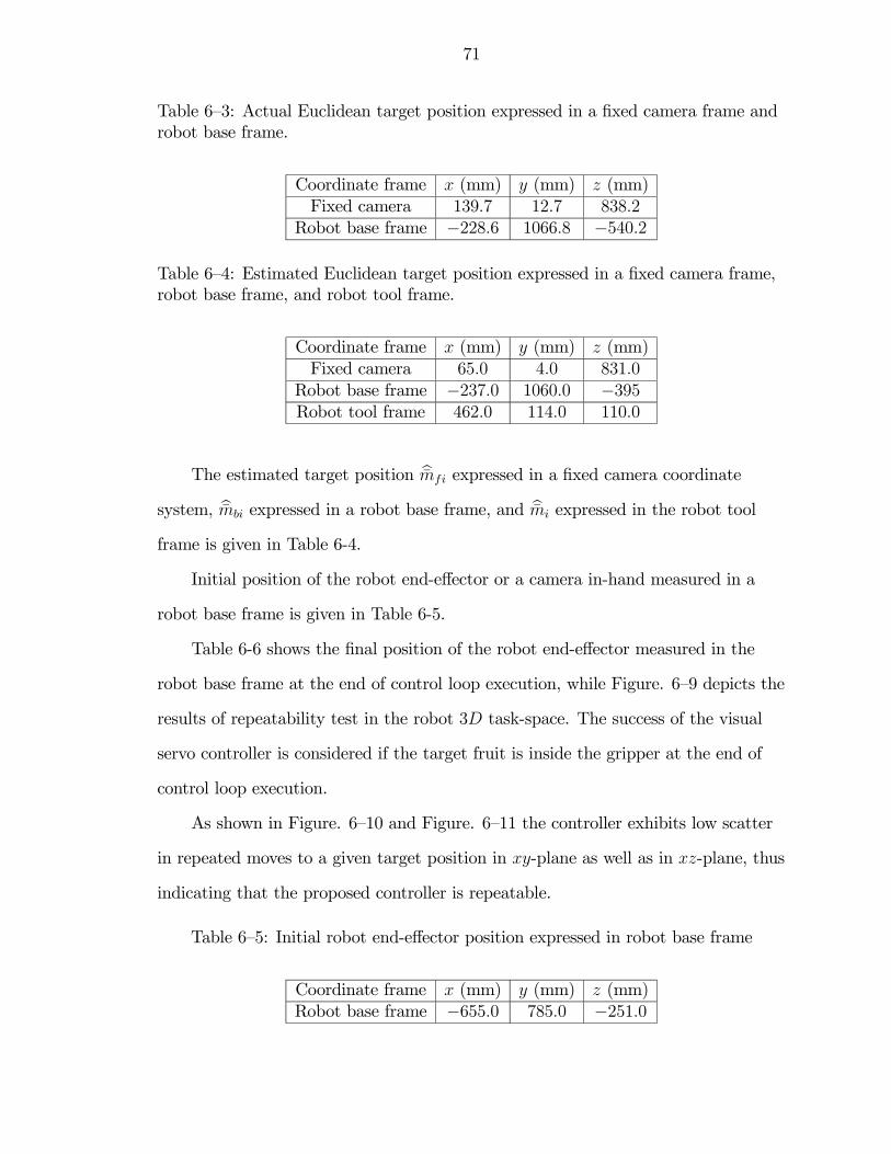
71

Table 6—3: Actual Euclidean target position expressed in a fixed camera frame androbot base frame.

Coordinate frame x (mm) y (mm) z (mm)Fixed camera 139.7 12.7 838.2

Robot base frame −228.6 1066.8 −540.2

Table 6—4: Estimated Euclidean target position expressed in a fixed camera frame,robot base frame, and robot tool frame.

Coordinate frame x (mm) y (mm) z (mm)Fixed camera 65.0 4.0 831.0

Robot base frame −237.0 1060.0 −395Robot tool frame 462.0 114.0 110.0

The estimated target position bmfi expressed in a fixed camera coordinate

system, bmbi expressed in a robot base frame, and bmi expressed in the robot tool

frame is given in Table 6-4.

Initial position of the robot end-effector or a camera in-hand measured in a

robot base frame is given in Table 6-5.

Table 6-6 shows the final position of the robot end-effector measured in the

robot base frame at the end of control loop execution, while Figure. 6—9 depicts the

results of repeatability test in the robot 3D task-space. The success of the visual

servo controller is considered if the target fruit is inside the gripper at the end of

control loop execution.

As shown in Figure. 6—10 and Figure. 6—11 the controller exhibits low scatter

in repeated moves to a given target position in xy-plane as well as in xz-plane, thus

indicating that the proposed controller is repeatable.

Table 6—5: Initial robot end-effector position expressed in robot base frame

Coordinate frame x (mm) y (mm) z (mm)Robot base frame −655.0 785.0 −251.0

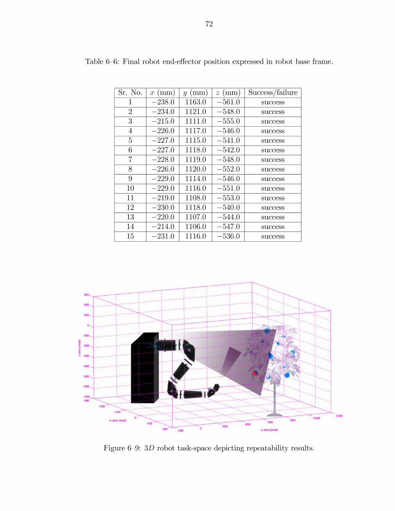
72

Table 6—6: Final robot end-effector position expressed in robot base frame.

Sr. No. x (mm) y (mm) z (mm) Success/failure1 −238.0 1163.0 −561.0 success2 −234.0 1121.0 −548.0 success3 −215.0 1111.0 −555.0 success4 −226.0 1117.0 −546.0 success5 −227.0 1115.0 −541.0 success6 −227.0 1118.0 −542.0 success7 −228.0 1119.0 −548.0 success8 −226.0 1120.0 −552.0 success9 −229.0 1114.0 −546.0 success10 −229.0 1116.0 −551.0 success11 −219.0 1108.0 −553.0 success12 −230.0 1118.0 −540.0 success13 −220.0 1107.0 −544.0 success14 −214.0 1106.0 −547.0 success15 −231.0 1116.0 −536.0 success

Figure 6—9: 3D robot task-space depicting repeatability results.

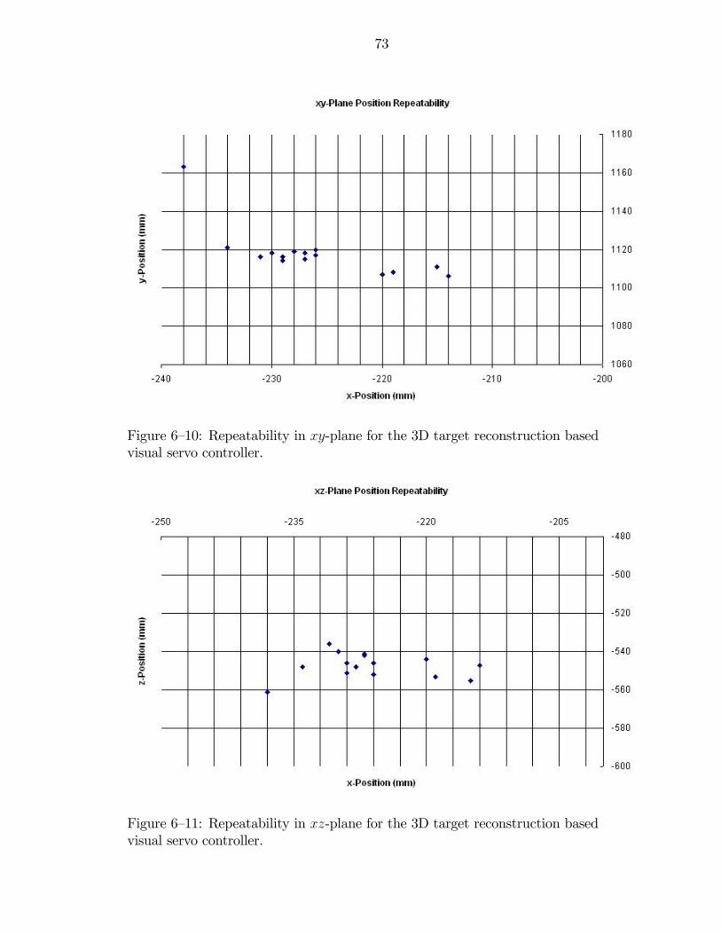
73

Figure 6—10: Repeatability in xy-plane for the 3D target reconstruction basedvisual servo controller.

Figure 6—11: Repeatability in xz-plane for the 3D target reconstruction basedvisual servo controller.

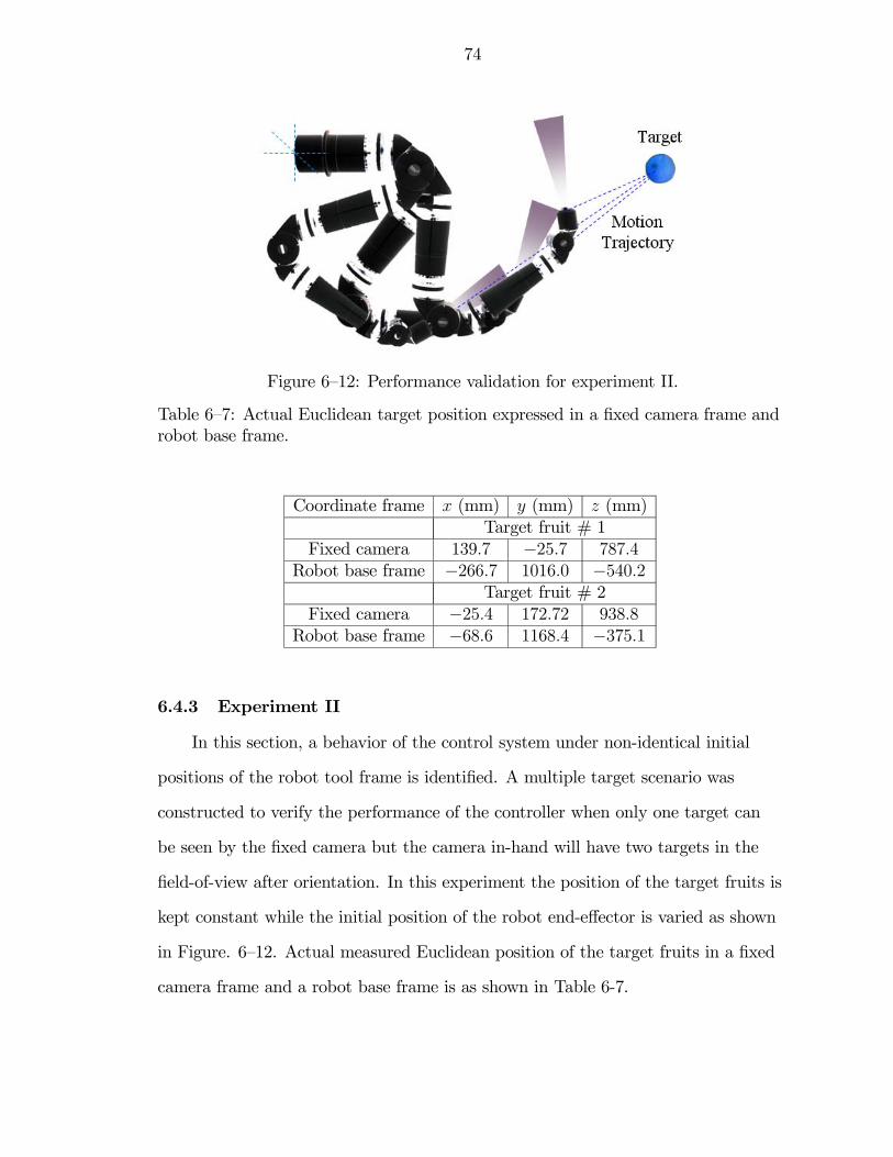
74

Figure 6—12: Performance validation for experiment II.

Table 6—7: Actual Euclidean target position expressed in a fixed camera frame androbot base frame.

Coordinate frame x (mm) y (mm) z (mm)Target fruit # 1

Fixed camera 139.7 −25.7 787.4Robot base frame −266.7 1016.0 −540.2

Target fruit # 2Fixed camera −25.4 172.72 938.8

Robot base frame −68.6 1168.4 −375.1

6.4.3 Experiment II

In this section, a behavior of the control system under non-identical initial

positions of the robot tool frame is identified. A multiple target scenario was

constructed to verify the performance of the controller when only one target can

be seen by the fixed camera but the camera in-hand will have two targets in the

field-of-view after orientation. In this experiment the position of the target fruits is

kept constant while the initial position of the robot end-effector is varied as shown

in Figure. 6—12. Actual measured Euclidean position of the target fruits in a fixed

camera frame and a robot base frame is as shown in Table 6-7.

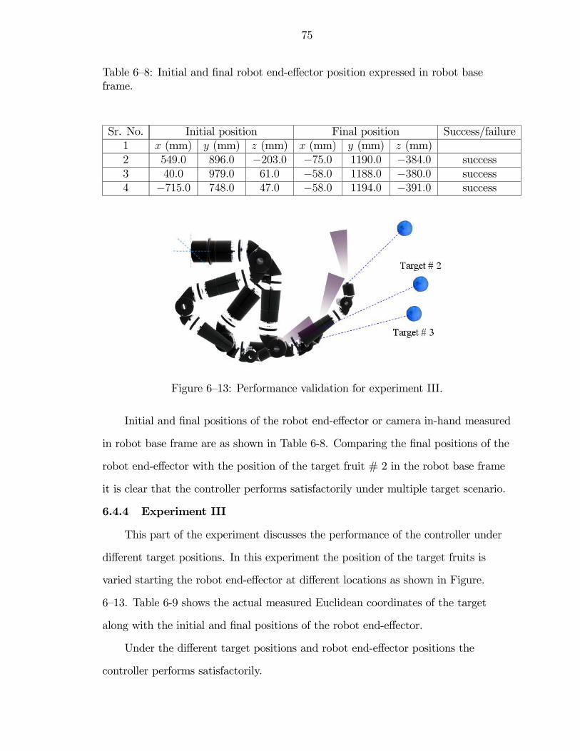
75

Table 6—8: Initial and final robot end-effector position expressed in robot baseframe.

Sr. No. Initial position Final position Success/failure1 x (mm) y (mm) z (mm) x (mm) y (mm) z (mm)2 549.0 896.0 −203.0 −75.0 1190.0 −384.0 success3 40.0 979.0 61.0 −58.0 1188.0 −380.0 success4 −715.0 748.0 47.0 −58.0 1194.0 −391.0 success

Figure 6—13: Performance validation for experiment III.

Initial and final positions of the robot end-effector or camera in-hand measured

in robot base frame are as shown in Table 6-8. Comparing the final positions of the

robot end-effector with the position of the target fruit # 2 in the robot base frame

it is clear that the controller performs satisfactorily under multiple target scenario.

6.4.4 Experiment III

This part of the experiment discusses the performance of the controller under

different target positions. In this experiment the position of the target fruits is

varied starting the robot end-effector at different locations as shown in Figure.

6—13. Table 6-9 shows the actual measured Euclidean coordinates of the target

along with the initial and final positions of the robot end-effector.

Under the different target positions and robot end-effector positions the

controller performs satisfactorily.

76

Table 6—9: Actual Euclidean target position expressed in a fixed camera frame androbot base frame and initial and final robot end-effector position expressed in robotbase frame.

Sr. No. Target fruit position Target fruit position(Fixed camera frame) (Robot base frame)

x (mm) y (mm) z (mm) x (mm) y (mm) z (mm)1 139.7 −25.4 787.4 −266.7 1016.0 −540.22 139.7 12.7 838.2 −228.6 1066.8 −540.23 127.9 −171.6 782.55 −412.6 1011.4 −528.9

Sr. No. Initial position Final position Success(Robot base frame) (Robot base frame) /failure

x (mm) y (mm) z (mm) x (mm) y (mm) z (mm)1 −138.0 1015 −223 −272.0 964.0 −563.0 success2 −538.0 554.0 −920.0 −240.0 900.0 −471.0 success3 39.0 981.0 69.0 −416.0 952.0 −514.0 success

6.5 Conclusion

A 3D target reconstruction based visual servo control approach is proposed

for robotic citrus harvesting where a prior knowledge of the feature points is not

available and feature point matching does not perform satisfactorily thus rendering

feature point matching-based teach by zooming visual servo control impractical.

3D target reconstruction method utilizes statistical data of the target size along

with the camera intrinsic parameters to generate an estimate for the Euclidean

position of a target. A 3D depth estimation method performs satisfactorily for

targets attributing larger depths from the camera frame and hence the control

algorithm is switched from vision-based to IR-based when the camera in-hand

is closer to the target. The controller exhibits very high success rate in terms of

accurately reaching the target, and also the repeatability test shows good position

repeatability in xy and xz-plane.

CHAPTER 7CONCLUSION

7.1 Summary of Results

Automated robotic citrus harvesting yields superior fruit quality, which is

highly desirable for fresh fruit market. The presented work accomplishes two

important characteristics of the automated fruit harvesting system, namely to

locate the fruits on the three dimensional space and to approach and reach for the

fruit. Color thresholding-based technique is realized for target fruit identification,

whereas multi-camera visual servo control techniques, viz. teach by zooming

visual servo control and 3D target reconstruction based visual servo control, are

developed for 3D target position estimation and robot motion control.

A teach by zooming visual servo control approach is proposed for applications

where the camera cannot be a priori positioned to the desired position/orientation

to acquire a desired image before servo control. Specifically, the teach by zooming

control objective is formulated to position/orient an on-board camera based on a

reference image obtained by another camera. In addition to formulating the teach

by zooming control problem, another contribution of this work is to illustrate how

to preserve a symmetric transformation from the projective homography to the

Euclidean homography for problems when the corresponding images are taken from

different cameras with calibration uncertainty. Simulation results are provided to

illustrate the performance of the controller. Rotation and translation errors are

exponentially regulated to zero thus establishing the stability of the controller,

whereas the angular and linear control velocities are always bounded. Applications

of this strategy could include navigating ground or air vehicles, based on desired

images taken by other ground or air vehicles.

77

78

Practical limitation on the implementation of the teach by zooming visual

servo controller for the citrus harvesting application has been realized in the

fact that the feature points viewed by the fixed camera can be different than the

feature points viewed by the camera in-hand. Non-identical feature points between

the current image and the desired image would result in incorrect rotation and

translation information. Hence the teach by zooming visual servo controller can

be implemented where the feature point information is available a priori, i.e. this

controller is suitable for artificial targets.

A 3D target reconstruction-based visual servo control approach is realized

for robotic citrus harvesting where a prior knowledge of the feature points is not

available and feature point matching does not perform satisfactorily thus rendering

feature point matching-based teach by zooming visual servo control impractical.

Specifically, statistical data of the target size is used for 3D target reconstruction

for generating an estimate for the Euclidean position of a target. A 3D depth

estimation method performs satisfactorily for targets attributing larger depths

from the camera frame and hence the control algorithm is switched from vision-

based to IR-based when the camera in-hand is closer to the target. The controller

exhibits very high success rate in terms of accurately reaching the target, also the

repeatability test shows good position repeatability in xy and xz-plane. Moreover,

the image-based visual servo control along with the Euclidean depth information

is used and hence the controller is robust to the target statistical data as well as

camera calibration parameters.

7.2 Recommendations for Future Work

One of the issues with teach by zooming visual servo controller is of consis-

tently identifying at least four feature points, which are necessary for homography

decomposition to acquire rotation and translation information between various

camera coordinate frames. This issue can be addressed by projecting an artificial

79

grid on the target and acquiring feature points on the grid. A prior knowledge of a

grid segment can also be utilized for target depth estimation. Non-identical feature

point matching issue can be resolved by using an artificial grid to consistently ob-

tain feature points on the target and controlling the trajectory of a camera in-hand

such that fixed camera as well as camera in-hand obtain identical feature points.

Multi-view photogrammetry techniques works under the assumption that

the four feature points are coplanar points. Image segmentation and texture

recognition techniques can be used to recognize different planes which would

help in defining the region of interest of the feature detection algorithm to ensure

feature points are coplanar. This would also make the tracker more consistent

and reliable to intensity variations in the scene. Another issue to be addressed

is to make sure that the points selected are not collinear. Also, the condition of

the four feature points required to be coplanar and collinear can be eliminated by

implementing the eight point algorithm proposed in [16], where the feature points

don’t have to satisfy the mentioned constraints.

Target detection task is primarily performed by a fixed camera mounted on

a stationary robot base joint and camera in-hand is servoed based on the selected

target. Target detection efficiency can be enhanced by performing the target

detection by fixed camera as well as camera in-hand. Moreover, simultaneous

localization and mapping (SLAM) of target fruits can be achieved by performing

the detection task by a camera in-hand along with a fixed camera in order to

generate a three dimensional map of the scene for efficient harvesting.

APPENDIX AOPEN-LOOP ERROR DYNAMICS

A.1 Rotation Controller

A rotation error-like signal, denoted by eω (t) ∈ R3, is defined by the angle axis

representation in (5—34) as follows:

eω = uθ. (A—1)

Taking the derivative of (A—1) with respect to time

deωdt

=d(uθ)

dt= uθ + uθ. (A—2)

Multiplying equation (A—2) by (I + u2×) and using properties of a skew

symmetric matrix the following expression can be obtained:

(I + u2×)d(uθ)

dt= uθ (A—3)

where I ∈ R3×3 denotes an identity matrix and u× denotes the 3×3 skew-symmetric

matrix associated with u(t).

Similarly, multiplying equation (A—2) by (−u2×) we get,

(−u2×)d(uθ)

dt= uθ. (A—4)

The angular velocity, expressed in the current camera frame, is defined as

follows:

ωc× = R(u, θ)RT (u, θ). (A—5)

80

81

From (5—36) and utilizing the properties of a skew symmetric matrix the

expression for ωc× in (A—5) can be written as follows:

ωc× = sin θu× + u×θ + (1− cos θ)(u×u)× (A—6)

where ωc× ∈ R3×3 denotes the 3× 3 skew-symmetric matrix associated with ωc(t).

Utilizing the properties developed in (A—3) and (A—4), the expression for

angular velocity ωc can be obtained as,

ωc = uθ + [sin θI + (1− cos θ)u×]u

= uθ + [sin θI +θ

2sin c2

θ

2u×]uθ

= [I +θ

2sin c2

θ

2u× + (1− sin θ)u2×]| {z } d(uθ)dt

(A—7)

L−1ω (u, θ)

where the Jacobian matrix Lω (t) ∈ R3×3 is defined as follows:

Lω = (L−1ω )

−1 = I +θ

2sin c2

θ

2u× + (1− sin θ)u2×. (A—8)

In equation (A—7) the sin c(θ) term is given by (A—8) as,

sin c(θ) =sin(θ)

θ. (A—9)

Based on the camera extrinsic parameters given in (5—33) and expression

(A—7), the open-loop error dynamics can be obtained as follows:

eω =d(uθ)

dt= LωRrωr. (A—10)

82

A.2 Translation Controller

The difference between the actual and desired 3D Euclidean camera position,

denoted by the translation error signal ev (t) ∈ R3, is defined as

ev , me −mde (A—11)

where me (t) ∈ R3 denotes the extended coordinates of an image point on π

expressed in terms of F and mde ∈ R3 denotes the extended coordinates of the

corresponding desired image point on π in terms of Fd given in (5—52) and (5—53),

respectively.

Taking the derivative of ev in (A—11) with respect to time

ev =

⎡⎢⎢⎢⎢⎢⎢⎣X1

Z1− X1

Z21Z1

Y1Z1− Y1

Z21Z1

Z1Z1

⎤⎥⎥⎥⎥⎥⎥⎦

ev =1

Z1

⎡⎢⎢⎢⎢⎢⎣1 0 −X1

Z1

0 1 −Y1Z1

0 0 1

⎤⎥⎥⎥⎥⎥⎦⎡⎢⎢⎢⎢⎣

X1

Y1

Z1

⎤⎥⎥⎥⎥⎦

ev =1

Z1

⎡⎢⎢⎢⎢⎢⎣1 0 −X1

Z1

0 1 −Y1Z1

0 0 1

⎤⎥⎥⎥⎥⎥⎦ υc − Lυ [m1]x ωc

ev =1

Z1

⎡⎢⎢⎢⎢⎢⎣1 0 −X1

Z1

0 1 −Y1Z1

0 0 1

⎤⎥⎥⎥⎥⎥⎦ υc −1

Z1

⎡⎢⎢⎢⎢⎢⎣−X1Y1

Z1−Z1 −−

X21

Z1Y1

Z1 +Y 21

Z1−X1Y1

Z1−X1

−Y1 X1 0

⎤⎥⎥⎥⎥⎥⎦ωc

ev = LvRrvr + λw¡Lv [tr]× + Lvω

¢Rreω (A—12)

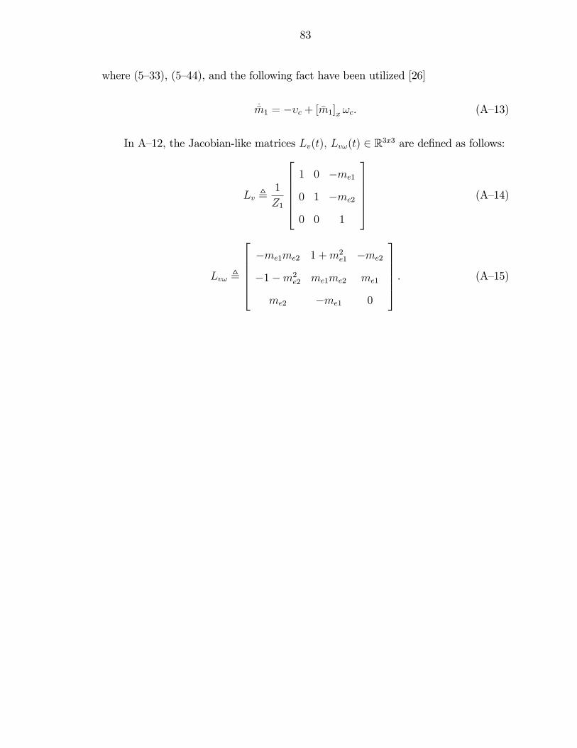
83

where (5—33), (5—44), and the following fact have been utilized [26]

.m1 = −υc + [m1]x ωc. (A—13)

In A—12, the Jacobian-like matrices Lv(t), Lvω(t) ∈ R3x3 are defined as follows:

Lv ,1

Z1

⎡⎢⎢⎢⎢⎣1 0 −me1

0 1 −me2

0 0 1

⎤⎥⎥⎥⎥⎦ (A—14)

Lvω ,

⎡⎢⎢⎢⎢⎣−me1me2 1 +m2

e1 −me2

−1−m2e2 me1me2 me1

me2 −me1 0

⎤⎥⎥⎥⎥⎦ . (A—15)

APPENDIX BTARGET IDENTIFICATION AND FEATURE POINT TRACKING

ALGORITHM

B.1 Target Detection

//*******************************************************************

// PROGRAM START

//*******************************************************************

//*******************************************************************

// What this program does:

// 1) Detects target (citrus) based on color thresholding principle

// for the image taken by fixed camera as well as camera in-hand.

// 2) Estimates the target region area along with the diameter and depth of

the target.

// What is the input to this program:

// The input is sequence of images (i.e. real-time video) taken using two

cameras

// What is the output of this program:

// Target region area, target diameter, estimate of target depth

// The code given below does not include the entire program used for the

autonomous

// robotic citrus harvester, but shows the important functions.

//*******************************************************************

#include "StdAfx.h"

#include "ImagProcFunctions.h"

#include <fstream.h>

84

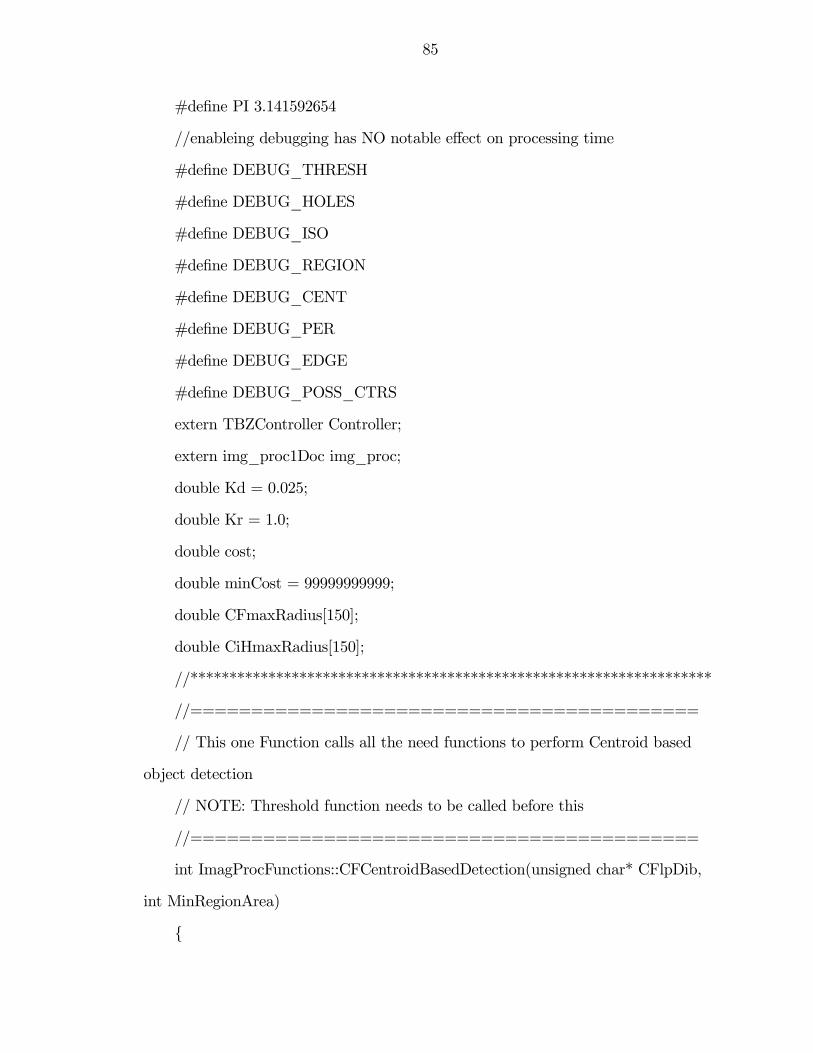
85

#define PI 3.141592654

//enableing debugging has NO notable effect on processing time

#define DEBUG_THRESH

#define DEBUG_HOLES

#define DEBUG_ISO

#define DEBUG_REGION

#define DEBUG_CENT

#define DEBUG_PER

#define DEBUG_EDGE

#define DEBUG_POSS_CTRS

extern TBZController Controller;

extern img_proc1Doc img_proc;

double Kd = 0.025;

double Kr = 1.0;

double cost;

double minCost = 99999999999;

double CFmaxRadius[150];

double CiHmaxRadius[150];

//*******************************************************************

//==========================================

// This one Function calls all the need functions to perform Centroid based

object detection

// NOTE: Threshold function needs to be called before this

//==========================================

int ImagProcFunctions::CFCentroidBasedDetection(unsigned char* CFlpDib,

int MinRegionArea)

{

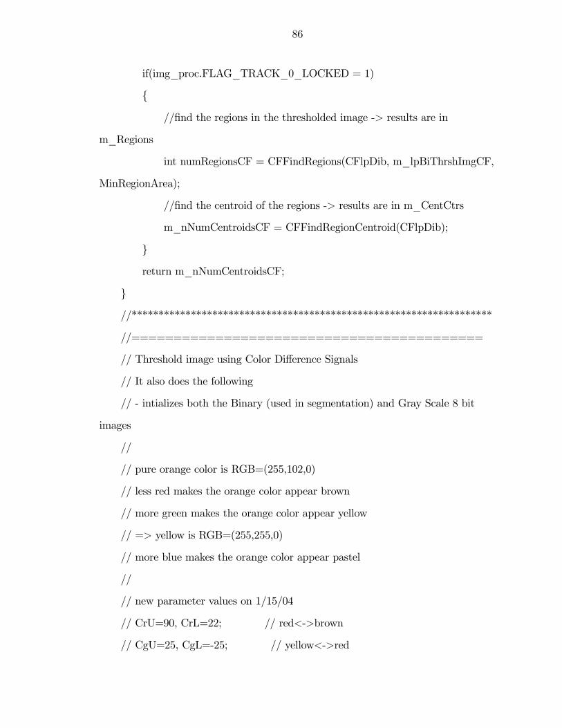
86

if(img_proc.FLAG_TRACK_0_LOCKED = 1)

{

//find the regions in the thresholded image -> results are in

m_Regions

int numRegionsCF = CFFindRegions(CFlpDib, m_lpBiThrshImgCF,

MinRegionArea);

//find the centroid of the regions -> results are in m_CentCtrs

m_nNumCentroidsCF = CFFindRegionCentroid(CFlpDib);

}

return m_nNumCentroidsCF;

}

//*******************************************************************

//==========================================

// Threshold image using Color Difference Signals

// It also does the following

// - intializes both the Binary (used in segmentation) and Gray Scale 8 bit

images

//

// pure orange color is RGB=(255,102,0)

// less red makes the orange color appear brown

// more green makes the orange color appear yellow

// => yellow is RGB=(255,255,0)

// more blue makes the orange color appear pastel

//

// new parameter values on 1/15/04

// CrU=90, CrL=22; // red<->brown

// CgU=25, CgL=-25; // yellow<->red

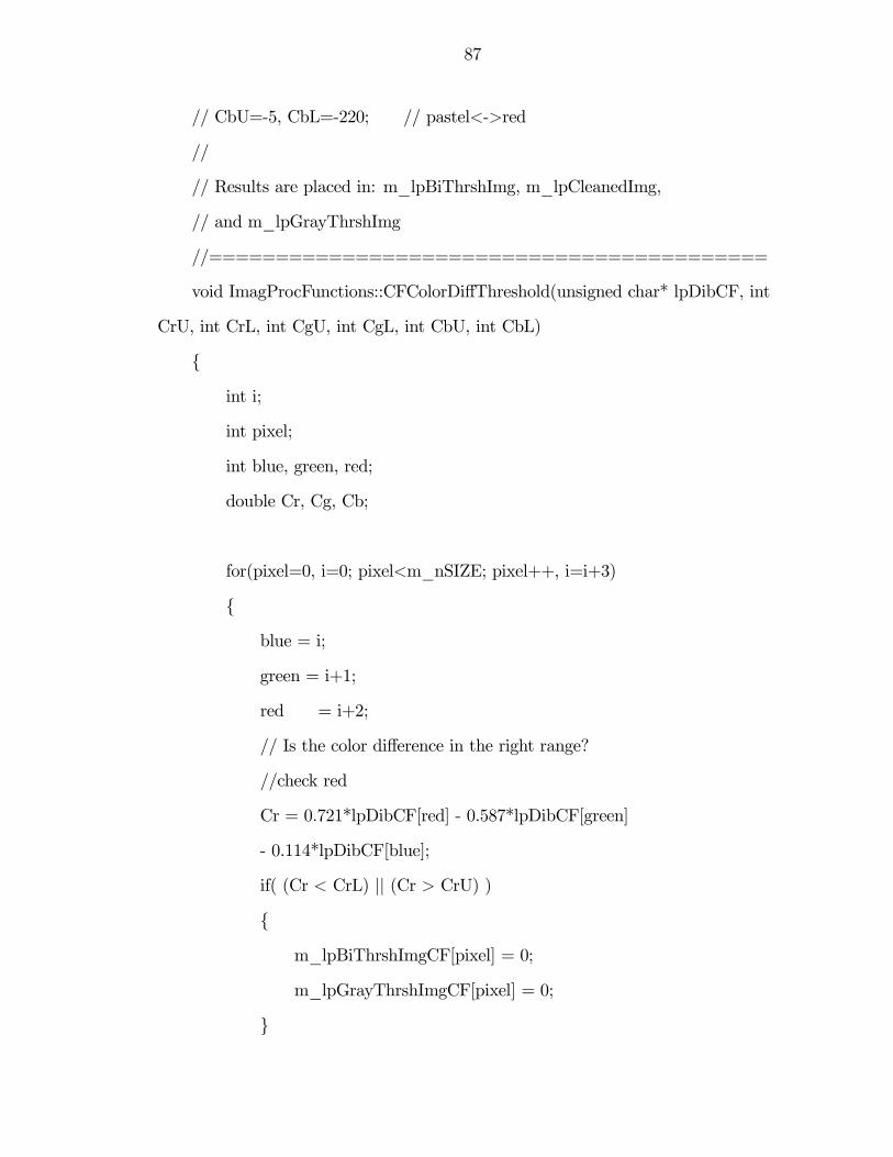
87

// CbU=-5, CbL=-220; // pastel<->red

//

// Results are placed in: m_lpBiThrshImg, m_lpCleanedImg,

// and m_lpGrayThrshImg

//==========================================

void ImagProcFunctions::CFColorDiffThreshold(unsigned char* lpDibCF, int

CrU, int CrL, int CgU, int CgL, int CbU, int CbL)

{

int i;

int pixel;

int blue, green, red;

double Cr, Cg, Cb;

for(pixel=0, i=0; pixel<m_nSIZE; pixel++, i=i+3)

{

blue = i;

green = i+1;

red = i+2;

// Is the color difference in the right range?

//check red

Cr = 0.721*lpDibCF[red] - 0.587*lpDibCF[green]

- 0.114*lpDibCF[blue];

if( (Cr < CrL) || (Cr > CrU) )

{

m_lpBiThrshImgCF[pixel] = 0;

m_lpGrayThrshImgCF[pixel] = 0;

}

88

else

{

//check green

Cg = -0.299*lpDibCF[red] + 0.413*lpDibCF[green]

- 0.114*lpDibCF[blue];

if( (Cg < CgL) || (Cg > CgU) )

{



}

else

{

//check blue

Cb = -0.299*lpDibCF[red] - 0.587*lpDibCF[green]

+ 0.886*lpDibCF[blue];

if( (Cb < CbL) || (Cb > CbU) )

{



}

else

{


// it can take up to an extra 6-8ms to do this calcula-

tion for the image

89

m_lpGrayThrshImgCF[pixel] = (unsigned char)(0.299*lpDibCF[red] +

0.587*lpDibCF[green] + 0.114*lpDibCF[blue]);

//this is just for display

//color the pixel in the original image

#ifdef DEBUG_THRESH

lpDibCF[blue] = 255;

lpDibCF[green] = 0;

lpDibCF[red] = 0;

#endif

}

}

}

}

}

//*******************************************************************

//==========================================

// A queue-based paint-fill routine for color image using 4 connectivity

// MinRegionArea is the minimum region that is desired

// Returns the number of regions found => This can also be found in

m_nNumRegs

// Finds the following:

// -> coords to these regions can be found in m_lpRegCoords

// -> the region’s size (# of pixels) is in m_nRegSize

// -> the memory offset of the region’s pixels is in m_nRegMemOffset

// -> the pixel closest to the origin for each region is in m_nRegMinCoord

//==========================================

90

int ImagProcFunctions::CFFindRegions(unsigned char* CFlpDib, unsigned

char* CFimage, int MinRegionArea)

{

int i;

int pixel;

int qh, qt;

int count;

int minCoord;

unsigned char paintOverLabel=255, newPaintLabel=1;


#ifdef DEBUG_REGION

int cPix;

#endif

// Loop through binary image looking for regions

m_RegionsCF[0].memOffset = 0;

m_nNumRegsCF = 0;

//start checking

for(i=0; i<m_nSIZE; i++)

{

// Check to see if initial/seed pixel is not a background pixel

if( (CFimage[i] == paintOverLabel) && (m_nNumRegsCF <

MAX_REGIONS) )

{

// seed pixel is not background => save info on it

CFimage[i] = newPaintLabel;

91

m_lpRegPixQueueCF[0] = i;

m_lpRegCoordsCF[ m_RegionsCF[m_nNumRegsCF].

memOffset ] = i;

//init varaibles

count = 1;

qh = 1;

qt = 0;

minCoord = i;

// start looking for other pixels around seed pixel

// the loop will exit after it circles around and finds only itself as

a viable pixel

while (qt != qh)

{

// look below

pixel = m_lpRegPixQueueCF[qt]-m_nCOL;

//make sure coordinate is in image AND it is not a back-

ground pixel

if( (m_lpRegPixQueueCF[qt]/m_nCOL > 0) && (CFim-

age[pixel] == paintOverLabel) )

{

// Set new found pixel to newPaintLabel

CFimage[pixel] = newPaintLabel;

// Save new found pixels coordinates and intensity


memOffset + count ] = pixel;

92

// check to see if it is the closest to the origin

if( pixel < minCoord )

{

minCoord = pixel;

}

// increment number of pixels in region

count++;

// set next pixel in queue to search as the pixel that

was just found

m_lpRegPixQueueCF[qh] = pixel;

// check to see if we have reached the max number of

coords

// a%b will always return a if a < b

// this statement also increments qh by 1

qh = (qh+1)%MAX_REG_COORDS;

}

pixel = m_lpRegPixQueueCF[qt]+m_nCOL;

if (m_lpRegPixQueueCF[qt]/m_nCOL < m_nROW-1 &&

CFimage[pixel] == paintOverLabel)

{





{

93

minCoord = pixel;

}

count++;



}

pixel = m_lpRegPixQueueCF[qt]-1;

if (m_lpRegPixQueueCF[qt]%m_nCOL > 0 && CFim-

age[pixel] == paintOverLabel)

{





{

minCoord = pixel;

}

count++;



}

pixel = m_lpRegPixQueueCF[qt]+1;

94

if (m_lpRegPixQueueCF[qt]%m_nCOL < m_nCOL-1 &&

CFimage[pixel] == paintOverLabel)

{





{

minCoord = pixel;

}

count++;



}

qt++;

}

// Check region

// make sure area is large enough

// if area is too small erase it from image

// make sure not to write outside arrays

if( (count > MinRegionArea) && (m_nNumRegsCF <

MAX_REGIONS) )

{

// save the number of pixels in region

// array starts at 0 and num of regions starts at 1 => do

this step before incrementing num of regions

95

m_RegionsCF[m_nNumRegsCF].area = count;

// save pixel that is closest to origin

m_RegionsCF[m_nNumRegsCF].minCoord = minCoord;

// save region’s label

m_RegionsCF[m_nNumRegsCF].label = newPaintLabel;

// increment the number of useful regions

m_nNumRegsCF++;

// set offset for next set of coordinates

m_RegionsCF[m_nNumRegsCF].memOffset = count +

m_RegionsCF[m_nNumRegsCF-1].memOffset;

// set new paint label

newPaintLabel = newPaintLabel++;

}

else

{

//not a viable region so delete it from image

for(pixel=0; pixel<count; pixel++)

{

CFimage[ m_lpRegCoordsCF[ m_RegionsCF

[m_nNumRegsCF].memOffset + pixel ] ] = 0;

m_lpGrayThrshImgCF[ m_lpRegCoordsCF

[m_RegionsCF[m_nNumRegsCF].memOffset + pixel ] ]

= 0;


//color the pixel in the original image

#ifdef DEBUG_REGION

96

cPix = 3*m_lpRegCoordsCF[ m_RegionsCF

[m_nNumRegsCF].memOffset + pixel ];

CFlpDib[cPix] = 0;

CFlpDib[cPix + 1] = 0;

CFlpDib[cPix + 2] = 255; //red

#endif

}

}

}

}

return m_nNumRegsCF;

}

//*******************************************************************

//==========================================

// Finds the centroid (aka center of mass) of the previously found regions

// the location of the centroid is saved in 2D as a gray scale pixel number not

RGB

//==========================================

int ImagProcFunctions::CFFindRegionCentroid(unsigned char* CFlpDib)

{

int reg, pixel;

int x, y;

int numCent=0;

m_nAvgObjDiameter = 67.1576;

#ifdef DEBUG_CENT

int cPix;

int r,c,temp;

97

#endif

//loop through all the regions

for(reg=0; reg<m_nNumRegsCF; reg++)

{

// col=>x and row=>y for bottom up DIB

x = 0;

y = 0;

//add up all coords in region

//for(pixel=0; pixel<m_nRegSize[reg]; pixel++)

for(pixel=0; pixel<m_RegionsCF[reg].area; pixel++)

{

x += m_lpRegCoordsCF[ m_RegionsCF[reg].memOffset + pixel

]%m_nCOL;

y += m_lpRegCoordsCF[ m_RegionsCF[reg].memOffset + pixel

]/m_nCOL;

}

//average values to get centroid

m_CentCtrsCF[reg].Xp[0] = x/m_RegionsCF[reg].area;

m_CentCtrsCF[reg].Xp[1] = y/m_RegionsCF[reg].area;

//find distance centroid is from center of image (note: 0,0 is not the

center of the image)

m_CentCtrsCF[reg].dist = (int)sqrt( pow(m_CentCtrsCF[reg].Xp[0]-

(m_nCOL/2),2) + pow(m_CentCtrsCF[reg].Xp[1]-(m_nROW/2),2) );

//the is no radius associated with the centroid of a region

//assume regions is round, and thus from area = PI*radius^2 ->

radius = sqrt(area/PI)

98

m_CentCtrsCF[reg].radius = (int)sqrt(m_RegionsCF[reg].area/PI);

m_RegionsCF[reg].depth = (Controller.m_CFCalibrationMatrix.

m_Value[0][0]*m_nAvgObjDiameter)

/(2*2*m_CentCtrsCF[reg].radius);

// 2 times radius since the image is 320x240 instead of 640x480

m_RegionsCF[reg].cost = Kr*(320/m_CentCtrsCF[reg].radius - 1) +

Kd*m_RegionsCF[reg].depth;

//find lowest cost

if( m_RegionsCF[reg].cost < minCost )

{

minCost = m_RegionsCF[reg].cost;

m_RegionsCF[reg].number = 1;

m_HarvestFruit.RegionNumCF = reg;

}

if( m_CentCtrsCF[m_HarvestFruit.RegionNumCF].radius >

CFmaxRadius[m_HarvestFruit.RegionNumCF])

{

CFmaxRadius[m_HarvestFruit.RegionNumCF] =

m_CentCtrsCF[m_HarvestFruit.RegionNumCF].radius;

m_HarvestFruit.RadiusCF =

CFmaxRadius[m_HarvestFruit.RegionNumCF];

m_HarvestFruit.DepthCF= (Controller.m_CFCalibrationMatrix.

m_Value[0][0]*m_nAvgObjDiameter)

/(2*2*m_HarvestFruit.RadiusCF);

}

/*

OutputDebugString("\n");

99

OutputDebugString("Camera 0 ");

char radius[20];

itoa(m_HarvestFruit.RadiusCF,radius,10);

OutputDebugString(radius);

OutputDebugString(" ");

char depth[20];

itoa(m_HarvestFruit.DepthCF,depth,10);

OutputDebugString(depth);

OutputDebugString("\n");

*/

//increment the number of centroids found

numCent++;


//draw crosshairs

#ifdef DEBUG_CENT

temp = m_CentCtrsCF[reg].Xp[1]*m_nCOL

+ m_CentCtrsCF[reg].Xp[0];

for( r=-20; r<=20; r++ )

{

cPix = temp + r;

if( (cPix > 0) && (cPix < m_nSIZE) )

{

cPix = 3*cPix;

CFlpDib[cPix] = 0;



}

100

}

for( c=-20; c<=20; c++ )

{

cPix = temp + c*m_nCOL;

if( (cPix > 0) && (cPix < m_nSIZE) )

{

cPix = 3*cPix;

CFlpDib[cPix] = 0;



}

}

#endif

}

return numCent;

}

//*******************************************************************

//==========================================

// Transform Pixel Coordinates to Camera Coordinates

// - Xp are the supplied pixel coordinates in a 2 element array (xp,yp)

// - distanceInch is the ditance to the scene in inches

// - Xn are the normal coords -> the have no units and require the range for

any real use

// - Xc is the returned 3 element array with camera coordinates in inches

(xc,yc,zc)

//

101

// The Z axis for Xc is the line of sight of the camera: Xp=(0,0) => Xc=(-

xc,-yc)

// The center of the camera frame is the principle point in pixel frame:

Xp=(ppx,ppy) => Xc = (0,0)

//==========================================

void ImagProcFunctions::TransformCoordsInv (int* Xp, double distanceInch,

double* Xn, double* Xc)

{

int i;

double R2, R4, R6, K;

double old[2], delta[2];

//get data

m_Xp.m_Value[0][0] = Xp[0];

m_Xp.m_Value[1][0] = Xp[1];

m_Xp.m_Value[2][0] = 1;

//convert from pixel coords to distortion coords

m_CamMatInv = m_CameraMatrix^-1;

m_Xd = m_CamMatInv*m_Xp;

//convert from distortion coords to normal coords

m_Xn = m_Xd; //initial guess -> normal = distortion

for( i=0; i<20; i++ )

{

old[0] = m_Xn.m_Value[0][0];

old[1] = m_Xn.m_Value[1][0];

R2 = pow(m_Xn.m_Value[0][0], 2) + pow(m_Xn.m_Value[1][0], 2);

R4 = R2*R2;

R6 = R2*R4;

102

K = 1/(1 + m_dKcCiH[0]*R2 + m_dKcCiH[1]*R4

+ m_dKcCiH[4]*R6);

//X = Xd - dX

m_Xn.m_Value[0][0] = m_Xd.m_Value[0][0] -

( 2*m_dKcCiH[2]*m_Xn.m_Value[0][0]*m_Xn.m_Value[1][0]

+ m_dKcCiH[3]*(R2 + 2*m_Xn.m_Value[0][0]

*m_Xn.m_Value[0][0]) );

m_Xn.m_Value[1][0] = m_Xd.m_Value[1][0] -

(m_dKcCiH[2]*(R2 + 2*m_Xn.m_Value[1][0]*m_Xn.m_Value[1][0])

+ 2*m_dKcCiH[3]*m_Xn.m_Value[0][0]*m_Xn.m_Value[1][0] );

m_Xn.m_Value[2][0] = 1;

//Xn = K*X

m_Xn = m_Xn*K;

delta[0] = fabs(m_Xn.m_Value[0][0] - old[0]);

delta[1] = fabs(m_Xn.m_Value[1][0] - old[1]);

}

m_Xn.m_Value[2][0] = 1;

//return values to Xn array

Xn[0] = m_Xn.m_Value[0][0];

Xn[1] = m_Xn.m_Value[1][0];

//convert from normal coords to camera coords (distance needs to be in

centimeters)

m_Xc = m_Xn*distanceInch;

Xc[0] = m_Xc.m_Value[0][0];


103


}

//*******************************************************************

// PROGRAM END

//*******************************************************************

B.2 Feature Point Tracking

//*******************************************************************

// PROGRAM START

//*******************************************************************

//*******************************************************************


// 1) Detects feature points in the given image based on the differential

intensity along

// x and y-axis.

// 2) Tracks the feature points from one frame to the next


// The input is sequence of images (i.e. real-time video) taken using two

cameras


// Pixel coordinates of the tracked feature points

// The code given below does not include the entire program used for the

autonomous

// robotic citrus harvester, but shows the important functions.

//*******************************************************************

#pragma once

#include <StdAfx.h>

#include "cv.h"

104

#include "highgui.h"

#include "FPTracking.h"

#include <windef.h>

extern TBZController Controller;

extern img_proc1Doc img_proc;

extern CitrusDetection CitrusDetect;

extern LinearAlgebra m_CiHHarvestFruitPixCoord;

extern LinearAlgebra m_CFHarvestFruitPixCoord;

#ifdef _DEBUG

#undef THIS_FILE

static char THIS_FILE[]=__FILE__;

#define new DEBUG_NEW

#endif

#define PI 3.1415926535897932384626433832795;

// Variables:

const int sobel = 1; // image size in Ipl

int th_fp = 5000, // threshold for feature point

detection

Wx = 7, // x-dir tracking window size

(pixels)

Wy = 7, // y-dir tracking window size

(pixels)

x_lim = 10, // x-dir minimum distance for

feature points (pixels)

y_lim = 10, // y-dir minimum distance for

feature points (pixels)

105

border_x = 10, // horizontal image border -

pixels (this region is not processed)

border_y = 10, // vertical image border -

pixels (this region is not processed)

fp0[320*240][2], // array of possible feature point

locations

fp1[320*240][2], // array of possible feature point

locations

n_res = 3, // number of resolutions

(current max is 3 due to programming limitations)

bound_x = (Wx-1)/2,

bound_y = (Wy-1)/2,

LostFeatCount = 0,

CtrImg_horz = 80,

CtrImg_vert = 60;

double track_tol = .1, // convergence criteria for

tracker (pixels)

fp_s0[320*240], // minimum eigenvalues for

possible feature point locations

fp_s1[320*240]; // minimum eigenvalues for

possible feature point locations

//*******************************************************************

// FUNCTION — get_feature_points0 for CAMERA 0

// get_feature_points0 : Finds the feature points in the image based on Sobel

filter

//*******************************************************************

void FPTracking::get_feature_points0(IplImage* img)

106

{

if (img_proc.FLAG_TRACK_1_LOCKED == 0)

{

img_proc.FLAG_TRACK_0_LOCKED = 1;

double Ixx, Iyy, Ixy, single[2], s_min;

int fp_count = 0;

// initialize image derivative arrays

Ix_0 = cvCreateImage(img_proc.proc_size,IPL_DEPTH_32F,1);

Iy_0 = cvCreateImage(img_proc.proc_size,IPL_DEPTH_32F,1);

cvSobel(img,Ix_0,1,0,sobel);

cvSobel(img,Iy_0,0,1,sobel);

// slide window over entire image (minus borders)

for (int i=border_x+bound_x+(img_proc.n_horz-CtrImg_horz)/2;

i<img_proc.n_horz - border_x-bound_x-1-(img_proc.n_horz-CtrImg_horz)/2;

i++)

{

for (int j=border_y+bound_y+(img_proc.n_vert-CtrImg_vert)

/2; j<img_proc.n_vert - border_y-bound_y-1

-(img_proc.n_vert-CtrImg_vert)/2; j++)

{

// set region of interest

CvRect window = cvRect( i, j, Wx, Wy );

cvSetImageROI( Ix_0, window );

cvSetImageROI( Iy_0, window );

// calculate G

Ixx = cvDotProduct(Ix_0,Ix_0);

107

Iyy = cvDotProduct(Iy_0,Iy_0);

Ixy = cvDotProduct(Ix_0,Iy_0);

CvMat G,s;

double temp[2][2] = {{Ixx,Ixy},{Ixy,Iyy}};

cvInitMatHeader( &G, 2, 2, CV_64FC1, temp );

// Singular value decomposition

s=cvMat( 2, 1, CV_64FC1,single);

cvSVD(&G,&s);

s_min = cvGetReal1D(&s,1);

if (s_min > th_fp)

{

fp0[fp_count][0] = i+bound_x;

fp0[fp_count][1] = j+bound_y;

fp_s0[fp_count] = s_min;

fp_count++;

}

}

}

cvResetImageROI(Ix_0);

cvResetImageROI(Iy_0);

cvReleaseImage(&Ix_0);

cvReleaseImage(&Iy_0);

// sort fp0 and fp_s0 arrays into descending order

sortDescend0(fp0,fp_s0,fp_count);

}

else


108

}

//*******************************************************************

// FUNCTION — track_multi_res0 for CAMERA 0

// track_multi_res0 : Feature poont tracking function based on multi-

resolution KLT algorithm

//*******************************************************************

void FPTracking::track_multi_res0(IplImage* img_prev_0, IplImage*

img_curr_0,int got_features, int frame_count)

{

if (img_proc.FLAG_TRACK_1_LOCKED == 0)

{


double x,y,xn,yn,xi,yi,xf,yf,boundx_res,boundy_res,

borderx_res,bordery_res;

double Ixx_sub, Iyy_sub, Ixy_sub,Ixt_sub,Iyt_sub,

temp_G[4],temp_b[2],d[2],d0[2];

int xr,yr,n_horz_c,n_vert_c;

CvSize res_size; // image size in Ipl format

CvSize win_size = cvSize(Wx,Wy); // window size in Ipl format

CvMat d_mat,G,b;

int track_pts=0;

int sumx = 0;

int sumy = 0;

int CtrImg_CtrX;

int CtrImg_CtrY;

Ix_0 = cvCreateImage(img_proc.proc_size,IPL_DEPTH_32F,1);

Iy_0 = cvCreateImage(img_proc.proc_size,IPL_DEPTH_32F,1);

109

cvSobel(img_prev_0,Ix_0,1,0,sobel);

cvSobel(img_prev_0,Iy_0,0,1,sobel);

// create decimated images

if (n_res > 0)

{

n_horz_c = img_proc.n_horz / (int)pow(2,1);

n_vert_c = img_proc.n_vert / (int)pow(2,1);

res_size = cvSize(n_horz_c,n_vert_c);

img_curr_1 = cvCreateImage(res_size,IPL_DEPTH_32F,1);

img_prev_1 = cvCreateImage(res_size,IPL_DEPTH_32F,1);

cvResize( img_prev_0, img_prev_1,CV_INTER_AREA);

cvResize( img_curr_0, img_curr_1,CV_INTER_AREA);

Ix_1 = cvCreateImage(res_size,IPL_DEPTH_32F,1);

Iy_1 = cvCreateImage(res_size,IPL_DEPTH_32F,1);



}

if (n_res > 1)

{









110




}

if (n_res > 2)

{











cvSobel(img_curr_3,Iy_3,0,1,sobel);

}

// loop for all feature points

for (int i = 0; i < img_proc.tracked_pts0; i++)

{

// round past feature point locations

x = fpts0[i][0];

y = fpts0[i][1];

d[0] = 0;

d[1] = 0;

xn = x;

111

yn = y;

xr = (int)(x+.5);

yr = (int)(y+.5);

// multiscale loop (image is equal to original when res = 0)

if ((xr>border_x+bound_x) && (xr<img_proc.n_horz -

border_x-bound_x-1) && (yr>border_y+bound_y) && (yr<img_proc.n_vert-

border_y-bound_y-1))

{

for(int res=n_res; res>=0; res—)

{

// calculate number of pixels for course grid

n_horz_c = img_proc.n_horz / (int)pow(2,res);

n_vert_c = img_proc.n_vert / (int)pow(2,res);

// determine feature point location in course grid

xi = (x / pow(2,res))+ 0.5 - (1 / pow(2,res+1));

yi = (y / pow(2,res))+ 0.5 - (1 / pow(2,res+1));

xf = (xn / pow(2,res)) + 0.5 - (1 / pow(2,res+1));

yf = (yn / pow(2,res)) + 0.5 - (1 / pow(2,res+1));

boundx_res = bound_x/pow(2,res);

boundy_res = bound_y/pow(2,res);

borderx_res = border_x/pow(2,res);

bordery_res = border_x/pow(2,res);

CvPoint2D32f pt_i = cvPoint2D32f( xi, yi );

CvPoint2D32f pt_f = cvPoint2D32f( xf, yf );

// calculate only if feature point is in the image

if ( (floor(xf)-boundx_res-borderx_res >= 0)

112

&& (ceil(xf)+boundx_res+borderx_res <

n_horz_c)

&& (floor(xi)-boundx_res-borderx_res >= 0)

&& (ceil(xi)+boundx_res+borderx_res <

n_horz_c)

&& (floor(yf)-boundy_res-bordery_res >= 0)

&& (ceil(yf)+boundy_res+bordery_res <

n_vert_c)

&& (floor(yi)-boundy_res-bordery_res >= 0)

&& (ceil(yi)+boundy_res+bordery_res <

n_vert_c))

{

if (res == 0)

{

Ix_sub = cvCreateImage

(win_size,IPL_DEPTH_32F,1);

cvGetRectSubPix(Ix_0,Ix_sub,pt_i);

Iy_sub = cvCreateImage


cvGetRectSubPix(Iy_0,Iy_sub,pt_i);

img_curr_sub = cvCreateImage


cvGetRectSubPix

(img_prev_0,img_curr_sub,pt_i);

img_prev_sub = cvCreateImage


cvGetRectSubPix

113

(img_curr_0,img_prev_sub,pt_f);

It_sub = cvCreateImage


cvSub(img_curr_sub,img_prev_sub,It_sub);

// calculate G and b

Ixx_sub = cvDotProduct(Ix_sub,Ix_sub);

Iyy_sub = cvDotProduct(Iy_sub,Iy_sub);

Ixy_sub = cvDotProduct(Ix_sub,Iy_sub);

Ixt_sub = cvDotProduct(Ix_sub,It_sub);

Iyt_sub = cvDotProduct(Iy_sub,It_sub);;

temp_G[0] = Ixx_sub;

temp_G[1] = Ixy_sub;


temp_G[3] = Iyy_sub;

temp_b[0] = Ixt_sub;

temp_b[1] = Iyt_sub;

cvInitMatHeader( &G, 2, 2, CV_64FC1,

temp_G );

cvInitMatHeader( &b, 2, 1, CV_64FC1,

temp_b );

// solve for course displacement

if ((cvDet(&G) > 1) || (cvDet(&G) < 1))

{

d0[0] = 0;

d0[1] = 0;

cvInitMatHeader( &d_mat, 2, 1,

CV_64FC1,d0);

114

cvSolve(&G,&b,&d_mat,CV_SVD);

d0[0] = cvGetReal1D( &d_mat, 0 );


d[0] = d[0] + d0[0]*pow(2,res);

d[1] = d[1] + d0[1]*pow(2,res);

xn = x + d[0];

yn = y + d[1];

}

else

{

d0[0] = 0;

d0[1] = 0;

}

}

if (res == 1)

{









cvGetRectSubPix



115


cvGetRectSubPix










Iyt_sub = cvDotProduct(Iy_sub,It_sub);








temp_G );


temp_b );


if ((cvDet(&G) > 1) || (cvDet(&G) < 1))

{

d0[0] = 0;

d0[1] = 0;

116


CV_64FC1,d0);




d[0] = d[0] + d0[0]*pow(2,res);

d[1] = d[1] + d0[1]*pow(2,res);

xn = x + d[0];

yn = y + d[1];

}

else

{

d0[0] = 0;

d0[1] = 0;

}

}

if (res == 2)

{









cvGetRectSubPix

117




cvGetRectSubPix


















temp_G );


temp_b );


if ((cvDet(&G) > 1) || (cvDet(&G) < 1))

{

118

d0[0] = 0;

d0[1] = 0;


CV_64FC1,d0);




d[0] = d[0] + d0[0]*pow(2,res);

d[1] = d[1] + d0[1]*pow(2,res);

xn = x + d[0];

yn = y + d[1];

}

else

{

d0[0] = 0;

d0[1] = 0;

}

}

if (res == 3)

{








119


cvGetRectSubPix




cvGetRectSubPix


















temp_G );


temp_b );


120

if ((cvDet(&G) > 1) || (cvDet(&G) < 1))

{

d0[0] = 0;

d0[1] = 0;


CV_64FC1,d0);

cvSolve(&G,&b,&d_mat,CV_LU);



d[0] = d[0] + d0[0]*pow(2,res);

d[1] = d[1] + d0[1]*pow(2,res);

xn = x + d[0];

yn = y + d[1];

}

else

{

d0[0] = 0;

d0[1] = 0;

}

}

}

else continue;

cvReleaseImage(&Ix_sub);

cvReleaseImage(&Iy_sub);

cvReleaseImage(&It_sub);

121


cvReleaseImage(&img_curr_sub);

cvReleaseImage(&img_prev_sub);

}

xn = x + d[0];

yn = y + d[1];

// iteration step for sub_pixel accuraccy

double normd = sqrt(d[0]*d[0] + d[1]*d[1]);

// if there is some displacement

if (normd>0)

{

int test1 = 0;

int test2 = 0;

while ((test1 == 0) && (test2 < 10))

{

CvPoint2D32f pt_n = cvPoint2D32f( xn, yn );

CvPoint2D32f pt_i = cvPoint2D32f( x, y );

// calculate only if feature point is in the image

if ( (floor(xn)-bound_x-border_x >= 0)

&& (ceil(xn)+bound_x+border_x <

img_proc.n_horz)

&& (floor(yn)-bound_y-border_y >= 0)

&& (ceil(yn)+bound_y+border_y <

img_proc.n_vert))

{

122

// printf("FEATURE IS INSIDE THE

IMAGE\n");









cvGetRectSubPix




cvGetRectSubPix

(img_curr_0,img_prev_sub,pt_n);










CvMat G0,b0;


123






cvInitMatHeader( &G0, 2, 2, CV_64FC1,

temp_G );

cvInitMatHeader( &b0, 2, 1, CV_64FC1,

temp_b );

if ((cvDet(&G0) > .001) || (cvDet(&G0) <

-.001))

{

d0[0] = 0;

d0[1] = 0;


CV_64FC1,d0);

cvSolve(&G0,&b0,&d_mat,CV_SVD);



double normd0 = sqrt(d0[0]*d0[0] +

d0[1]*d0[1]);

if (normd0<=track_tol)

{

d[0] = d[0] + d0[0];

d[1] = d[1] + d0[1];

test1=1;

}

124

else if ((normd0 >=0) &&

(normd0<999999))

{

d[0] = d[0] + d0[0];

d[1] = d[1] + d0[1];

xn = x + d[0];

yn = y + d[1];

test2++;

}

else

{

test2 = 99999999;

}

}

else

{

test2=100;

}






}

else

{

test2 = 99999999;

125

}

}

if (test1 == 1)

{

CvMat G0,s;





cvInitMatHeader( &G0, 2, 2, CV_64FC1, temp_G

);

if ((cvDet(&G0) > .001) || (cvDet(&G0) < -.001))

{

double single[2]={{0},{0}},s_min;

//Singular value decomposition

s=cvMat( 2, 1, CV_64FC1,single);

cvSVD(&G0,&s);

s_min = cvGetReal1D(&s,1);

if (s_min > th_fp)

{

x = x + d[0];

y = y + d[1];

if ((x>0) && (x < img_proc.n_horz) &&

(y > 0) && (y<img_proc.n_vert))

{

fpts0[track_pts][0] = x;

fpts0[track_pts][1] = y;

126

track_pts = track_pts + 1;

}

}

}

}

}

else

{

fpts0[track_pts][0] = x;

fpts0[track_pts][1] = y;

track_pts = track_pts + 1;

}

sumx = sumx + x;

sumy = sumy + y;

}

}

CtrImg_CtrX = sumx / track_pts;

CtrImg_CtrY = sumy / track_pts;



cvReleaseImage(&It_0);






if (n_res > 0)

127

{



cvReleaseImage(&img_curr_1);

cvReleaseImage(&img_prev_1);

}

if (n_res > 1)

{





}

if (n_res > 2)

{





}

img_proc.tracked_pts0 = track_pts;

}


}

//*******************************************************************

// PROGRAM END

//*******************************************************************

APPENDIX CTEACH BY ZOOMING VISUAL SERVO CONTROL ALGORITHM

//*******************************************************************

// PROGRAM START

//*******************************************************************

//*******************************************************************


// 1) Homography decomposition to find out rotation and translation matrices

// 2) Teach by zooming visual servo controller computes the rotation and

translation

// velocities for the robot based on homography decomposition results.


// Pixel data of the feature points tracked using KLT algorithm


// Rotation and translation velocities for the low level controller.

//*******************************************************************

#pragma once

// Header Files

#include "stdafx.h"

#include <stdlib.h>

#include <iostream.h>

#include <strstrea.h>

#include <cv.h>

#include "TBZController.h"

#include <gsl/gsl_linalg.h>

128

129

// Disable Warnings

#pragma warning ( disable : 4244 )



// Global Variables

static gsl_vector *gh_work;

static gsl_matrix *gh_u;

static gsl_vector *gh_s;

static gsl_matrix *gh_v;

static gsl_vector *gh_b;

static gsl_vector *gh_x;

static gsl_vector *dh_work;

static gsl_matrix *dh_u;

static gsl_vector *dh_s;

static gsl_matrix *dh_v;

// Definitions

#define ERROR_BOUND 0.00001

//*******************************************************************

// TBZ Main Controller

//*******************************************************************

void TBZController::TBZControlMain(double fpts[][2],int rw, int rh, int

frame_count, int OrgFeatIndex[])

{

// Declarations

double thetaP;

int PtTransController = 1;

double Lamda_V;

130

double Lamda_W = 2;

double fFunction;

double kno = 1;

double kn1 = 1;

double kn2 = 1;

double Zstar_hat = 1;

double Z_hat;

// Create TBZ Workspace (Memory Allocation)

// TBZCreateFixedTBZWorkspace(frame_count);

if (frame_count > 2)

TBZCreateTBZWorkspace();

// Initialize TBZ Controller

// TBZControllerInit();

// Read Target Pixel Coordinates

TBZTargetCoord(fpts, rw, rh, frame_count, OrgFeatIndex);

// Homography Decomposition Algorithm to Get Rotation and Transla-

tion Information

TBZHomography(frame_count);

// TBZ Controller

m_R_Trans.MatTranspose(m_R);

m_p1.Mat2Vector(1,m_pi);

m_m1 = m_InvCiHCalibrationMatrix * m_p1;

m_p1_star.Mat2Vector(1,m_pi_star);

m_m1_star = m_InvCiHCalibrationMatrix * m_p1_star;

// Angle-Axis Representation for the rotation matrix

double CosAngle = 0.5 * (m_R.MatTrace() - 1.0);

131

// Error Handling

if (CosAngle > 1.0)

CosAngle = 1.0;

else if (CosAngle < -1.0)

CosAngle = -1.0;

thetaP = acos(CosAngle);

m_uPx = m_R - m_R_Trans;

if (thetaP == 0)

m_uPx.MatScale(0);

else

m_uPx.MatScale(1/(2 * sin(thetaP)));

m_uP.MatAntiSkew(m_uPx);

// Depth Estimation

Z_hat = Zstar_hat / m_alpha.m_Value[PtTransController - 1][0];

// Image Lv Matrix

m_Lv.m_Value[0][0] = -1 / Z_hat;

m_Lv.m_Value[0][1] = 0;

m_Lv.m_Value[0][2] = m_m1.m_Value[0][0] / Z_hat;

m_Lv.m_Value[1][0] = 0;


m_Lv.m_Value[1][2] = m_m1.m_Value[1][0] / Z_hat;

m_Lv.m_Value[2][0] = 0;

m_Lv.m_Value[2][1] = 0;


m_LvTrans.MatTranspose(m_Lv);

// Image Lvww Matrix

132

m_Lvw.m_Value[0][0] = m_m1.m_Value[0][0] * m_m1.m_Value[1][0];

m_Lvw.m_Value[0][1] = -1 - (m_m1.m_Value[0][0] *

m_m1.m_Value[0][0]);

m_Lvw.m_Value[0][2] = m_m1.m_Value[1][0];

m_Lvw.m_Value[1][0] = 1 + (m_m1.m_Value[1][0] *

m_m1.m_Value[1][0]);

m_Lvw.m_Value[1][1] = -1 * m_m1.m_Value[0][0] *

m_m1.m_Value[1][0];

m_Lvw.m_Value[1][2] = -1 * m_m1.m_Value[0][0];

m_Lvw.m_Value[2][0] = -1 * m_m1.m_Value[1][0];

m_Lvw.m_Value[2][1] = m_m1.m_Value[0][0];

m_Lvw.m_Value[2][2] = 0;

// Translation Controller Gain Computation

fFunction = (1/3.0) * (0.5 * pow(m_m1.m_Value[0][0] , 2) +

0.5 * pow(m_m1.m_Value[1][0] , 2) +

1 - sqrt(pow(0.5 * pow(m_m1.m_Value[0][0] , 2) +

0.5 * pow(m_m1.m_Value[1][0] , 2) + 1 , 2) - 1));

Lamda_V = kno + pow(Z_hat , 2) / fFunction;

// Open Loop Error System

m_eW = m_uP * thetaP;

m_eV = m_m1 - m_m1_star;

m_eV.m_Value[2][0] = log(m_alpha.m_Value[PtTransController - 1][0]);

m_eV.MatDisplay("Open Loop Error for Translation Controller");

m_eW.MatDisplay("Open Loop Error for Rotation Controller");

// Control signals (Camera Linear and Angular Velocity Commands)

m_INTCALC1 = m_LvTrans * m_eV;

m_INTCALC2 = m_INTCALC1;

133

m_INTCALC1.MatScale(-1 * Lamda_V);

m_INTCALC2.MatScale(-1 * (kn1 * pow(Z_hat,2) + kn2 * pow(Z_hat,2)

* m_eV.VectorNorm()));

m_Vc = m_INTCALC1 + m_INTCALC2;

m_Wc = m_eW * Lamda_W;

// Display Camera velocities

m_Vc.MatDisplay("Camera Linear Velocity");

m_Wc.MatDisplay("Camera Angular Velocity");

// Control signals (Robot Linear and Angular Velocity Commands)

m_INTCALC6.MatAugment("row",m_Vc,m_Wc);

m_Vr = m_INTCALC4 * m_INTCALC6;

m_Wr = m_INTCALC5 * m_INTCALC6;

// Display Robot velocities

m_Vr.MatDisplay("Robot Linear Velocity");

m_Wr.MatDisplay("Robot Angular Velocity");

// File Write

// TBZResultFileWrite(frame_count);

// Release TBZ Workspace (Memory De-Allocation)

// TBZReleaseTBZWorkspace();

}

//*******************************************************************

// Read Target Pixel Values for Camera in-Hand (CiH) and Fixed Camera

(CF)

//*******************************************************************

void TBZController::TBZTargetCoord(double fpts[][2],int rw, int rh, int

frame_count, int OrgFeatIndex[])

134

{

if (frame_count == 1 && OrgFeatIndex[3] != 999)

{

m_pi_star.m_Value[0][0] = fpts[OrgFeatIndex[0]][0];


m_pi_star.m_Value[2][0] = 1;










}

m_pi.m_Value[0][0] = fpts[OrgFeatIndex[0]][0];


m_pi.m_Value[2][0] = 1;



m_pi.m_Value[2][1] = 1;



m_pi.m_Value[2][2] = 1;



135

m_pi.m_Value[2][3] = 1;

/*













m_pi.m_Value[0][0] = 201;

m_pi.m_Value[1][0] = 104;

m_pi.m_Value[2][0] = 1;

m_pi.m_Value[0][1] = 195;

m_pi.m_Value[1][1] = 120;

m_pi.m_Value[2][1] = 1;

m_pi.m_Value[0][2] = 195;

m_pi.m_Value[1][2] = 111;

m_pi.m_Value[2][2] = 1;

m_pi.m_Value[0][3] = 204;

m_pi.m_Value[1][3] = 120;

m_pi.m_Value[2][3] = 1; */

}

136

//*******************************************************************

// TBZ Homography Decomposition Using SVD (Get Gn and Alpha_g33)

//*******************************************************************

int TBZController::TBZGetHomographySVD()

{

int numPoints = 0;

numPoints = m_pi.Col();

if(m_alpha_g33.GetNumElements() != numPoints || m_pi_star.Col() !=

numPoints

|| m_pi_star.Row() != 3 || m_pi.Row() != 3)

{

cout << "[getHomographySVD]: Arguments have incorrect dimen-

sions." << endl;

cout << "start" << endl;

cout << m_alpha_g33.GetNumElements() << endl;

cout << m_pi.Col() << endl;

cout << m_pi_star.Col() << endl;

cout << m_pi.Row() << endl;

cout << m_pi.Row() << endl;

return -1;

}

for (int i = 1; i <= numPoints; i++)

{

int row = 2 * i - 1;

gsl_matrix_set(gh_u, row - 1, 0, m_pi_star.m_Value[0][i-1]);

137


gsl_matrix_set(gh_u, row - 1, 2, 1.0);




gsl_matrix_set(gh_u, row - 1, 6, -1.0 * m_pi_star.m_Value[0][i-1] *

m_pi.m_Value[0][i-1]);



gsl_vector_set(gh_b, row - 1, 1.0 * m_pi.m_Value[0][i-1]);

row = 2 * i;











gsl_vector_set(gh_b, row - 1, 1.0 * m_pi.m_Value[1][i-1]);

}

if( gsl_linalg_SV_decomp(gh_u, gh_v, gh_s, gh_work) )

return -1;

138

if(gsl_linalg_SV_solve(gh_u, gh_v, gh_s, gh_b, gh_x))

return -1;

// Extract eigen vector for the smallest eigen value

m_Gn.m_Value[0][0] = gsl_vector_get(gh_x, 0);








m_Gn.m_Value[2][2] = 1.0;

// compute alpha.G33 for each image correspondance

for (i = 0; i < numPoints; i++)

m_alpha_g33.m_Value[i][0] = 1.0/(m_Gn.m_Value[2][0] *

m_pi_star.m_Value[0][i] + m_Gn.m_Value[2][1] * m_pi_star.m_Value[1][i]

+ 1.0);

return 0;

}

//*******************************************************************

// Decompose Homography (Get Rotation and Translation)

//*******************************************************************

int TBZController::TBZDecomposeHomographySimple()

{

double sign;

double d_dash;

float st, ct; // sin(theta) and cos(theta). ’float’ type to

139

// avoid numerical errors

double scaleFactor; // the ’d’ in decomposition alg. p 290 faugeras

//–––––––––––––––––––

// Equations. See Faugeras for description of the algorithm

// R_bar = sign.U.R_dash.V^T

// x_f_bar = U.x_dash;

// n_star = V.n_dash;

// d_star = sign.d_dash;

//–––––––––––––––––––

for(int i=0; i<3; i++)

{

for(int j=0; j<3; j++)

{

gsl_matrix_set(dh_u, i, j, m_Hn.m_Value[i][j]);

}

}

//SVD of homography matrix

if( gsl_linalg_SV_decomp(dh_u, dh_v, dh_s, dh_work) )

return -1;

for (i = 0; i < 3; i++)

{

m_D.m_Value[i][0] = gsl_vector_get(dh_s, i);

for (int j = 0; j < 3; j++)

{

m_U.m_Value[i][j] = gsl_matrix_get(dh_u, i, j);

140

m_V.m_Value[i][j] = gsl_matrix_get(dh_v, i, j);

}

}

sign = m_U.MatDeterminant() * m_V.MatDeterminant();

m_TransV.MatTranspose(m_V);

m_n_dash = m_TransV * m_nstarActual;

// In this experiment the object is always visible to camera,

// hence distance to the object plane is always positive.

// This determines sign of d_dash.

scaleFactor = sign * m_D.m_Value[1][0];

if(scaleFactor >= 0)

d_dash = m_D.m_Value[1][0];

else

{

d_dash = -1 * m_D.m_Value[1][0];

scaleFactor = -1 * scaleFactor;

}

// Based on the sign of d_dash, find R_dash and x_dash

// NOTE: Using error bounds instead. Is 0.9999 = 1.0001?

if( (fabs(m_D.m_Value[0][0] - m_D.m_Value[1][0]) > ERROR_BOUND)

&& (fabs(m_D.m_Value[1][0] - m_D.m_Value[2][0]) > ERROR_BOUND) )

{

if( d_dash > 0)

{

st = (m_D.m_Value[0][0] - m_D.m_Value[2][0]) *

(m_n_dash.m_Value[0][0] * m_n_dash.m_Value[2][0])

/ m_D.m_Value[1][0];

141

ct = (m_D.m_Value[1][0] * m_D.m_Value[1][0] +

m_D.m_Value[0][0] * m_D.m_Value[2][0])

/(m_D.m_Value[1][0] * (m_D.m_Value[0][0]

+ m_D.m_Value[2][0]));

// set m_R_dash

m_R_dash.m_Value[0][0] = ct;

m_R_dash.m_Value[0][1] = 0;

m_R_dash.m_Value[0][2] = -1*st;




m_R_dash.m_Value[2][0] = st;



// set m_x_dash

m_x_dash.m_Value[0][0] = (m_D.m_Value[0][0] -

m_D.m_Value[2][0]) * m_n_dash.m_Value[0][0];

m_x_dash.m_Value[1][0] = 0;

m_x_dash.m_Value[2][0] = -1 * (m_D.m_Value[0][0] -

m_D.m_Value[2][0]) * m_n_dash.m_Value[2][0];

}

else

{

st = (m_D.m_Value[0][0] + m_D.m_Value[2][0]) *

(m_n_dash.m_Value[0][0] * m_n_dash.m_Value[2][0])

/ m_D.m_Value[1][0];

142

ct = (m_D.m_Value[0][0] * m_D.m_Value[2][0] -

m_D.m_Value[1][0] * m_D.m_Value[1][0])

/(m_D.m_Value[1][0] * (m_D.m_Value[0][0]

- m_D.m_Value[2][0]));

// set m_R_dash





m_R_dash.m_Value[1][1] = -1;




m_R_dash.m_Value[2][2] = -1*ct;

//set m_x_dash

m_x_dash.m_Value[0][0] = (m_D.m_Value[0][0]

+ m_D.m_Value[2][0]) * m_n_dash.m_Value[0][0];




}

}

// all equal singular values (pure rotation, mostly)

if((fabs(m_D.m_Value[0][0] - m_D.m_Value[1][0])<= ERROR_BOUND)

&& (fabs(m_D.m_Value[1][0] - m_D.m_Value[2][0]) <= ERROR_BOUND))

{

143

if(d_dash > 0)

{









m_R_dash.m_Value[2][2] = 1; // unit matrix




}

else

{

// m_R_dash = -I + 2n_dash.n_dash^T

m_R_dash.m_Value[0][0] = 2 * m_n_dash.m_Value[0][0] *

m_n_dash.m_Value[0][0] - 1;


m_n_dash.m_Value[1][0];





144











m_x_dash.m_Value[0][0] = (-2 * d_dash)

* m_n_dash.m_Value[0][0];


m_x_dash.m_Value[2][0] = (-2 * d_dash)

* m_n_dash.m_Value[2][0];

}

}

// two equal singular values (translation is normal to the plane)

if( (fabs(m_D.m_Value[0][0] - m_D.m_Value[1][0]) <= ERROR_BOUND)

|| (fabs(m_D.m_Value[1][0] - m_D.m_Value[2][0]) <= ERROR_BOUND) )

{

if(d_dash > 0)

{





145







- m_D.m_Value[0][0]) * m_n_dash.m_Value[0][0];



- m_D.m_Value[0][0]) * m_n_dash.m_Value[2][0];

}

else

{















146

}

}

m_R.MatMult(m_U, m_R_dash, m_TransV);

m_R = m_R * sign;

m_x_h = m_U * m_x_dash;

m_x_h = m_x_h * (1.0/scaleFactor);

if(m_alpha_g33.GetNumElements() != m_alpha.GetNumElements())

{

cout << "[decomposeHomographySimple]: Arguments have incorrect

dimensions." << endl;

return -1;

}

for(int index = 0; index < m_alpha_g33.GetNumElements(); index++)

m_alpha.m_Value[index][0] = m_alpha_g33.m_Value[index][0] *

scaleFactor;

return 0;

}

//*******************************************************************

// PROGRAM END

//*******************************************************************

APPENDIX DVISION-BASED 3D TARGET RECONSTRUCTION ALGORITHM

//*******************************************************************

// PROGRAM START

//*******************************************************************


// 1) Uses Microsoft DirectX to capture the images from the camera

// 2) Executes the harvesting sequence

// 3) Generates the control commands for the robot.


// Target region area, target diameter, and extimated target depth from the

camera coordinate system.


// Position and orientation error signals for the visual servo controller.

//*******************************************************************

// HEADER FILES

//*******************************************************************

#pragma once

#define DRAWDIB_INCLUDE_STRETCHDIB

#include "stdafx.h"

#include "img_proc1.h"

#include "img_proc1Doc.h"

#include "MainFrm.h"

#include "cv.h"

#include "highgui.h"

147

148

#include <wingdi.h>

#include "GraphBase.h"

#include "CitrusDetection.h"

#include "FPTracking.h"

#include "MainRobot.h"

#include "TBZController.h"

#include "ImagProcFunctions.h"

#include "hispeed.h"

#include "robresfun.h"

#include "robotics.h"

#include "C:\Sid\Common\SERIAL\FIG.h"

#ifdef _DEBUG

#define new DEBUG_NEW

#undef THIS_FILE

static char THIS_FILE[] = __FILE__;

#endif

//*******************************************************************

// GLOBAL DEFINITIONS

//*******************************************************************

#define PI 3.141593

#define PID2 1.570796

#define PID4 0.785398

#define DEG2RAD 0.01745329

#define RAD2DEG 57.2957795

#define MAXREACH 60.0

//*******************************************************************

// FUNCTION — SampleCB for CAMERA 0

149

// SampleCB is the frame callback function. It will be called on each

// frame when the video is being played.

// SampleTime: the time stamp of current frame

// pSample: the media sample containing the image data

//

// If you want to process the image frames, just add your own

// processing code in this function.

//*******************************************************************

class CSampleGrabberCB0 : public ISampleGrabberCB

{

public:

// The interface needed by ISampleGrabber Filter

// fake out any COM ref counting

STDMETHODIMP_(ULONG) AddRef() { return 2; }

STDMETHODIMP_(ULONG) Release() { return 1; }

// fake out any COM QI’ing

STDMETHODIMP QueryInterface(REFIID riid, void ** ppv)

{

if( riid == IID_ISampleGrabberCB || riid == IID_IUnknown )

{


*ppv = (void *) static_cast<ISampleGrabberCB*> ( this );

return NOERROR;

}

return E_NOINTERFACE;

}

// The frame callback function called on each frame

150

// We can add the processing code in this function

// STDMETHODIMP SampleCB(double SampleTime, IMediaSample *pSam-

ple);

// Another callback function. I am not using it now.

STDMETHODIMP BufferCB(double SampleTime, BYTE *pBuffer, long

BufferLen)

{

return E_NOTIMPL;

}

// We have to set the mediaType as initialization, we can not get it

// through the pSample->GetMediaType(), it will be NULL if the media

// type did not change.

AM_MEDIA_TYPE m_mediaType;

STDMETHODIMP SampleCB(double SampleTime, IMediaSample

*pSample)

{

// get current media type

VIDEOINFOHEADER *pvi = (VIDEOINFOHEADER *)

m_mediaType.pbFormat;

// Get data from rgb24 image

pSample->GetPointer(&pDataCF);

SampleImgSize = pSample->GetSize();

H_pDataCF_IP = GlobalAlloc(GMEM_MOVEABLE,(unsigned

long)SampleImgSize);

pDataCF_IP = (unsigned char*)GlobalLock(H_pDataCF_IP);

memcpy(pDataCF_IP,pDataCF,(unsigned int)SampleImgSize);

HarvestStep2();

151


FrameCount++;

return NOERROR;

}

};

CSampleGrabberCB0 CB0;

//*******************************************************************

// FUNCTION — HarvestStep1

// HarvestStep1 : Step 1 in harvesting operation

// All the functions are initialized

//*******************************************************************

void HarvestStep1()

{

if (OutputDebugStringStatus == true)

OutputDebugString("Harvest Step 1\n");

img_proc.proc_size = cvSize(320,240); // size of images to process

img_proc.n_fpts = 9; // desired number of feature

points to track

img_proc.n_horz= img_proc.proc_size.width; // image width

(pixels)

img_proc.n_vert= img_proc.proc_size.height; // image height (pixels)

img_proc.FLAG_TRACK_0_LOCKED = 0; // Flag

indicating the tracking for image from camera 0

img_proc.FLAG_TRACK_1_LOCKED = 0; // Flag

indicating the tracking for image from camera 1

img_proc.tracked_pts0; // number of tracked

feature points

152

img_proc.tracked_pts1; // number of tracked

feature points

img_proc.OrgFeatIndex[20];

img_proc.numTarg0;

img_proc.numTarg1;

//init camera tool frame matrix

m_CameraToolMatrix.Xi = 1;

m_CameraToolMatrix.Xj = 0;

m_CameraToolMatrix.Xk = 0;

m_CameraToolMatrix.Yi = 0;

m_CameraToolMatrix.Yj = 1;

m_CameraToolMatrix.Yk = 0;

m_CameraToolMatrix.Zi = 0;

m_CameraToolMatrix.Zj = 0;

m_CameraToolMatrix.Zk = 1;

m_CameraToolMatrix.X = +0.0;

m_CameraToolMatrix.Y = -2.1;

m_CameraToolMatrix.Z = +3.500;

//init gripper tool frame matrix

m_GripperToolMatrix.Xi = 1;

m_GripperToolMatrix.Xj = 0;

m_GripperToolMatrix.Xk = 0;

m_GripperToolMatrix.Yi = 0;

m_GripperToolMatrix.Yj = 1;

m_GripperToolMatrix.Yk = 0;

m_GripperToolMatrix.Zi = 0;

m_GripperToolMatrix.Zj = 0;

153

m_GripperToolMatrix.Zk = 1;

m_GripperToolMatrix.X = 0.0;

m_GripperToolMatrix.Y = 0.5;

//m_GripperToolMatrix.Z = 6.0;

m_GripperToolMatrix.Z = 3.5;

//User jog

m_bEnableUserJog = false;

m_UserJogFrame = TOOL;

m_dUserJogVel[0] = 0.0;







// Results Filename

char* filename = "Results.txt";

// Delete Previous Versions of the File

int FileCheck = remove(filename);

if (FileCheck != 0)

MessageBox(0,"Remove File: File not found","File Write Error",0);

// Initialize the TBZ controller and load the variables

Controller.TBZCreateFixedTBZWorkspace(1);

Controller.TBZCreateTBZWorkspace();

Controller.TBZControllerInit();

Controller.TBZReleaseTBZWorkspace();

154

//Intialize image processing

CitrusDetect.Init();

//Initialize MainRobot

Robot.Init();

}

//*******************************************************************

// FUNCTION — HarvestStep2 for Camera 0


// Orange detection and depth estimation for Camera 0

//*******************************************************************

void HarvestStep2()

{

int i;


double old[2], delta[2];



pDataCF_US = (unsigned char *)pDataCF;

img_proc.IPFlag = 0;

img_proc.numTarg0 = CitrusDetect.CFImgProc(CENTROID, pDat-

aCF_US, img_proc.IPFlag);

m_CFHarvestFruitPixCoord.CreateMemory(3,1);

m_CFHarvestFruitNormCoord.CreateMemory(3,1);

m_CFHarvestFruit3DCoord.CreateMemory(3,1);

m_CFHarvestFruitNormCoordInitGuess.CreateMemory(3,1);

155

m_CFHarvestFruitPixCoord.m_Value[0][0] = CitrusDetect.m_IP.

m_CentCtrsCF[CitrusDetect.m_IP.m_HarvestFruit.RegionNumCF].Xp[0];

m_CFHarvestFruitPixCoord.m_Value[1][0] = CitrusDetect.m_IP.

m_CentCtrsCF[CitrusDetect.m_IP.m_HarvestFruit.RegionNumCF].Xp[1];

m_CFHarvestFruitPixCoord.m_Value[2][0] = 1;

// Calculate the Normalized euclidean coordinates of the target fruit

m_CFHarvestFruitNormCoord = Controller.m_InvCFCalibrationMatrix

* m_CFHarvestFruitPixCoord;

m_CFHarvestFruitNormCoordInitGuess = m_CFHarvestFruitNormCoord;

img_proc.m_CFHarvestFruitRadius =

CitrusDetect.m_IP.m_HarvestFruit.RadiusCF;

for( i=0; i<20; i++ )

{

old[0] = m_CFHarvestFruitNormCoord.m_Value[0][0];

old[1] = m_CFHarvestFruitNormCoord.m_Value[1][0];

R2 = pow(m_CFHarvestFruitNormCoord.m_Value[0][0], 2) +

pow(m_CFHarvestFruitNormCoord.m_Value[1][0], 2);

R4 = R2*R2;

R6 = R2*R4;

K = 1/(1 + Controller.m_CFDistortion[0]*R2

+ Controller.m_CFDistortion[1]*R4

+ Controller.m_CFDistortion[4]*R6);

//X = Xd - dX

m_CFHarvestFruitNormCoord.m_Value[0][0]

= m_CFHarvestFruitNormCoordInitGuess.m_Value[0][0] - ( 2 *

Controller.m_CFDistortion[2] * m_CFHarvestFruitNormCoord.m_Value[0][0] *

156

m_CFHarvestFruitNormCoord.m_Value[1][0] + Controller.m_CFDistortion[3] *

(R2 + 2 * m_CFHarvestFruitNormCoord.m_Value[0][0] *

m_CFHarvestFruitNormCoord.m_Value[0][0]) );

m_CFHarvestFruitNormCoord.m_Value[1][0]

= m_CFHarvestFruitNormCoordInitGuess.m_Value[1][0] - ( Con-

troller.m_CFDistortion[2] * (R2 + 2 * m_CFHarvestFruitNormCoord.m_Value[1][0]

* m_CFHarvestFruitNormCoord.m_Value[1][0]) + 2 * Con-

troller.m_CFDistortion[3] * m_CFHarvestFruitNormCoord.m_Value[0][0] *

m_CFHarvestFruitNormCoord.m_Value[1][0] );

m_CFHarvestFruitNormCoord.m_Value[2][0] = 1;

//Xn = K*X

m_CFHarvestFruitNormCoord = m_CFHarvestFruitNormCoord*K;

delta[0] = fabs(m_CFHarvestFruitNormCoord.m_Value[0][0] -

old[0]);

delta[1] = fabs(m_CFHarvestFruitNormCoord.m_Value[1][0] -

old[1]);

}

m_CFHarvestFruitNormCoord.m_Value[2][0] = 1;

CitrusDetect.m_IP.m_HarvestFruit.CFn_X

= m_CFHarvestFruitNormCoord.m_Value[0][0];

CitrusDetect.m_IP.m_HarvestFruit.CFn_Y


CitrusDetect.m_IP.m_HarvestFruit.CFn_Z


157

// Calculate the three dimensional position and orientation of the target

fruit in the Euclidean space

m_CFHarvestFruit3DCoord = m_CFHarvestFruitNormCoord * Citrus-

Detect.m_IP.m_HarvestFruit.DepthCF;

CitrusDetect.m_IP.m_HarvestFruit.CFe_X

= -m_CFHarvestFruit3DCoord.m_Value[0][0];

CitrusDetect.m_IP.m_HarvestFruit.CFe_Y

= -m_CFHarvestFruit3DCoord.m_Value[1][0];

CitrusDetect.m_IP.m_HarvestFruit.CFe_Z

= m_CFHarvestFruit3DCoord.m_Value[2][0];

// Calc the target’s position in the robot’s base frame

// Conversion between camera’s left handed coordinate system to robot

base joint’s right handed coordinate system

CitrusDetect.m_IP.m_HarvestFruit.CFb_X

= CitrusDetect.m_IP.m_HarvestFruit.CFe_Y - 254.00;

CitrusDetect.m_IP.m_HarvestFruit.CFb_Y

= CitrusDetect.m_IP.m_HarvestFruit.CFe_Z + 196.85;

CitrusDetect.m_IP.m_HarvestFruit.CFb_Z

= -CitrusDetect.m_IP.m_HarvestFruit.CFe_X - 381.00;

HarvestStep3();

}

//*******************************************************************


// HarvestStep3 : Allign robot along the axis joining Fixed camera coordinate

system and centroid

// of the target fruit

//*******************************************************************

158

void HarvestStep3()

{

double linVel[] = {15.0, 15.0, 15.0};

double rotVel[] = {PI, PI, PI};

double vel[] = {15.0, PID2, 0.0};

double fVel[] = {0.0, 0.0, 0.0};

double alpha, beta;



m_RotationMatX.CreateMemory(3,3);

m_RotationMatY.CreateMemory(3,3);

RequestToolFeedback();

// Position of fruit with respect to tool frame after acounting for the

orientation of tool

CitrusDetect.m_IP.m_HarvestFruit.CFt_X

= m_laInvRobotFeedbackRot.m_Value[0][0]

*CitrusDetect.m_IP.m_HarvestFruit.CFt_X

+ m_laInvRobotFeedbackRot.m_Value[0][1]

*CitrusDetect.m_IP.m_HarvestFruit.CFt_Y


*CitrusDetect.m_IP.m_HarvestFruit.CFt_Z;

CitrusDetect.m_IP.m_HarvestFruit.CFt_Y =

m_laInvRobotFeedbackRot.m_Value[1][0]





159


CitrusDetect.m_IP.m_HarvestFruit.CFt_Z =

m_laInvRobotFeedbackRot.m_Value[2][0]






if (xRotationDone == false || yRotationDone == false)

{

// Rotation about X-axis to get the desired orientation

alpha = atan2(CitrusDetect.m_IP.m_HarvestFruit.CFt_Y, Citrus-

Detect.m_IP.m_HarvestFruit.CFt_Z); // Rotation about X-axis

m_RotationMatX.m_Value[0][0] = 1;




m_RotationMatX.m_Value[1][1] = cos(alpha);

m_RotationMatX.m_Value[1][2] = sin(alpha);


m_RotationMatX.m_Value[2][1] = -sin(alpha);

m_RotationMatX.m_Value[2][2] = cos(alpha);

m_RotationMatX = m_laRobotFeedbackRot * m_RotationMatX;

//Xt

m_DesiredMatrix.Xi = m_RotationMatX.m_Value[0][0];

m_DesiredMatrix.Xj = m_RotationMatX.m_Value[1][0];

m_DesiredMatrix.Xk = m_RotationMatX.m_Value[2][0];

160

//Yt

m_DesiredMatrix.Yi = m_RotationMatX.m_Value[0][1];

m_DesiredMatrix.Yj = m_RotationMatX.m_Value[1][1];

m_DesiredMatrix.Yk = m_RotationMatX.m_Value[2][1];

//Zt

m_DesiredMatrix.Zi = m_RotationMatX.m_Value[0][2];

m_DesiredMatrix.Zj = m_RotationMatX.m_Value[1][2];

m_DesiredMatrix.Zk = m_RotationMatX.m_Value[2][2];

// Desired X, Y, and Z coordinates

m_DesiredMatrix.X = m_laRobotFeedbackPos.m_Value[0][0];

m_DesiredMatrix.Y = m_laRobotFeedbackPos.m_Value[1][0];

m_DesiredMatrix.Z = m_laRobotFeedbackPos.m_Value[2][0];

// Command to move the robot to the set point position and

orientation

if (RobotMotionControlOn == true)

if (Robot.ServoToSetpoint(BASE, &m_DesiredMatrix, linVel,

rotVel))

xRotationDone = true;

}


// Position of fruit with respect to tool frame after acounting for the

orientation of tool

CitrusDetect.m_IP.m_HarvestFruit.CFt_X





161



CitrusDetect.m_IP.m_HarvestFruit.CFt_Y







CitrusDetect.m_IP.m_HarvestFruit.CFt_Z







if (xRotationDone == false || yRotationDone == false)

{

// Rotation about Y-axis to get the desired orientation

beta = -atan2(CitrusDetect.m_IP.m_HarvestFruit.CFt_X, Citrus-

Detect.m_IP.m_HarvestFruit.CFt_Z); // Rotation about Y-axis

m_RotationMatY.m_Value[0][0] = cos(beta);

m_RotationMatY.m_Value[0][1] = 0;

m_RotationMatY.m_Value[0][2] = -sin(beta);




162

m_RotationMatY.m_Value[2][0] = sin(beta);


m_RotationMatY.m_Value[2][2] = cos(beta);

m_RotationMatY = m_laRobotFeedbackRot * m_RotationMatY;

//Xt

m_DesiredMatrix.Xi = m_RotationMatY.m_Value[0][0];

m_DesiredMatrix.Xj = m_RotationMatY.m_Value[1][0];

m_DesiredMatrix.Xk = m_RotationMatY.m_Value[2][0];

//Yt

m_DesiredMatrix.Yi = m_RotationMatY.m_Value[0][1];

m_DesiredMatrix.Yj = m_RotationMatY.m_Value[1][1];

m_DesiredMatrix.Yk = m_RotationMatY.m_Value[2][1];

//Zt

m_DesiredMatrix.Zi = m_RotationMatY.m_Value[0][2];

m_DesiredMatrix.Zj = m_RotationMatY.m_Value[1][2];

m_DesiredMatrix.Zk = m_RotationMatY.m_Value[2][2];

// Desired X, Y, and Z coordinates

m_DesiredMatrix.X = m_laRobotFeedbackPos.m_Value[0][0];

m_DesiredMatrix.Y = m_laRobotFeedbackPos.m_Value[1][0];

m_DesiredMatrix.Z = m_laRobotFeedbackPos.m_Value[2][0];


orientation


if (Robot.ServoToSetpoint(BASE, &m_DesiredMatrix, linVel,

rotVel))

yRotationDone = true;

163

}

m_laRobotFeedbackRot.DeleteMemory();

m_laRobotFeedbackPos.DeleteMemory();

m_laInvRobotFeedbackRot.DeleteMemory();

m_RotationMatX.DeleteMemory();

m_RotationMatY.DeleteMemory();

m_bEndEffectorExtension.DeleteMemory();

m_tEndEffectorExtension.DeleteMemory();

if (xRotationDone == true && yRotationDone == true)

HarvestStep4();

}

//*******************************************************************



// Align centroid of the fruit to the image centre

// Approach the fruit

//*******************************************************************

void HarvestStep4()

{



double linVel[] = {15.0, 15.0, 15.0};

double rotVel[] = {PID2, PID2, PID2};

double vel[] = {15.0, PID2, 0.0};

double fVel[] = {0.0, 0.0, 0.0};

if (maxCiHFruitRadius < CitrusDetect.m_IP.m_HarvestFruit.RadiusCiH)

zPositionSet = false;

164

if (zPositionSet == false)

{

zOldFdbkPosition = m_DesiredMatrix.Z;

zDesiredPosition = m_CiHHarvestFruit3DCoord.m_Value[2][0];

maxCiHFruitRadius = CitrusDetect.m_IP.m_HarvestFruit.RadiusCiH;

zPositionSet = true;

}


m_CentroidAlignmentError[0] = Controller.m_CiHCalibrationMatrix

.m_Value[0][2] - CitrusDetect.m_IP.m_CentCtrsCiH

[CitrusDetect.m_IP.m_HarvestFruit.RegionNumCiH].Xp[0];

m_CentroidAlignmentError[1] = - Controller.m_CiHCalibrationMatrix

.m_Value[1][2] + CitrusDetect.m_IP.m_CentCtrsCiH


m_CentroidAlignmentError[2] = zDesiredPosition

- fabs(m_laRobotFeedbackPos.m_Value[2][0] - zOldFdbkPosition);

// Command to move the robot to the set point position and orientation

if (RobotMotionControlOn == true && CentroidAlign == false &&

HarvestPosReached == false)

if (Robot.CentroidAlignment(m_CentroidAlignmentError, linVel,

rotVel))

CentroidAlign = true;

m_laRobotFeedbackRot.DeleteMemory();

m_laRobotFeedbackPos.DeleteMemory();

m_laInvRobotFeedbackRot.DeleteMemory();

m_bEndEffectorExtension.DeleteMemory();

m_tEndEffectorExtension.DeleteMemory();

165

GlobalFree(H_pDataCF_IP);

if (m_CentroidAlignmentError[2] <= 457.2)

{

if (IRSensorBasedGuidance == true)

CentroidAlign = true; // Force CentroidAlign flag to true to get

the IR based guidance

if (IRSensorOn == false)

Beep(2000,300);

IRSensorOn = true;

HarvestStep5();

}

}

//*******************************************************************



// IR Sensor is used to provide the accurate range measurements

// Activate the gripper to pick the fruit

//*******************************************************************

void HarvestStep5()

{



double linVel[] = {15.0, 15.0, 15.0};

double rotVel[] = {PID2, PID2, PID2};

double vel[] = {15.0, PID2, 0.0};

double fVel[] = {0.0, 0.0, 0.0};

if (m_IRS <= 5300 && HarvestPosReached == false)

166

{

FIG.mc[0]=’C’;

FIG.mc[1]=0;

FIG.lpComm->Write(FIG.mc,1);

Sleep(5);

FIG.mc[0]=’G’;

FIG.mc[1]=0;


HarvestPosReached = true;

if (HarvestPosReached == true)

// Beep(2000,300);

// Wait for 3 seconds and then open the gripper

Sleep(8000);

FIG.mc[0]=’W’;

FIG.mc[1]=0;


Sleep(5);

FIG.mc[0]=’G’;

FIG.mc[1]=0;


R2.JointSpaceTrj(&zCnfLen, pzCmdMot, arJntTar, rAccTime,

rJntVelFacApp, rJntVelFacTar);

}

if (CentroidAlign == true && HarvestPosReached == false && IRSen-

sorBasedGuidance == true)

{


167

m_IRSensorGuidanceError[0] = Controller.m_CiHCalibrationMatrix

.m_Value[0][2] - CitrusDetect.m_IP.m_CentCtrsCiH


m_IRSensorGuidanceError[1] = - Controller.m_CiHCalibrationMatrix

.m_Value[1][2] + CitrusDetect.m_IP.m_CentCtrsCiH


m_IRSensorGuidanceError[2] = 20; // Could be any value since we

intend to move in z-direction till the IR sensor is activated


orientation


if (Robot.CentroidCorrection(m_IRSensorGuidanceError, linVel,

rotVel))

{

CentroidCorrectionDone = true;

}

if (RobotMotionControlOn == true && CentroidCorrectionDone ==

true)

Robot.IRSensorGuidance(m_IRSensorGuidanceError, linVel,

rotVel);

OutputDebugString("IR Guidance\n");

}

}

//*******************************************************************

// FUNCTION — HarvestStep6 for Camera 1

168


// Orange detection and feature point tracking for Camera 1

//*******************************************************************

void HarvestStep6()

{

int i;


double old1[2], delta1[2];



pDataCiH_US = (unsigned char *)pDataCiH;

img_proc.IPFlag = 1;

img_proc.numTarg1 = CitrusDetect.CiHImgProc(CENTROID, pDat-

aCiH_US, img_proc.IPFlag);

// Determine the approximate Euclidean coordinates of the target object

m_CiHHarvestFruitPixCoord.CreateMemory(3,1);

m_CiHHarvestFruitNormCoord.CreateMemory(3,1);

m_CiHHarvestFruit3DCoord.CreateMemory(3,1);

m_CiHHarvestFruitNormCoordInitGuess.CreateMemory(3,1);

m_CiHHarvestFruitPixCoord.m_Value[0][0] = CitrusDetect.m_IP

.m_CentCtrsCiH[CitrusDetect.m_IP.m_HarvestFruit.RegionNumCiH]

.Xp[0];

m_CiHHarvestFruitPixCoord.m_Value[1][0] = CitrusDetect.m_IP

.m_CentCtrsCiH[CitrusDetect.m_IP.m_HarvestFruit.RegionNumCiH]

.Xp[1];

m_CiHHarvestFruitPixCoord.m_Value[2][0] = 1;

169

m_CiHHarvestFruitNormCoord = Controller.m_InvCiHCalibrationMatrix

* m_CiHHarvestFruitPixCoord;

m_CiHHarvestFruitNormCoordInitGuess

= m_CiHHarvestFruitNormCoord;

img_proc.m_CiHHarvestFruitRadius = CitrusDetect.m_IP

.m_HarvestFruit.RadiusCiH;

for(i=0; i<20; i++ )

{

old1[0] = m_CiHHarvestFruitNormCoord.m_Value[0][0];

old1[1] = m_CiHHarvestFruitNormCoord.m_Value[1][0];

R2 = pow(m_CiHHarvestFruitNormCoord.m_Value[0][0], 2) +

pow(m_CiHHarvestFruitNormCoord.m_Value[1][0],2);

R4 = R2*R2;

R6 = R2*R4;

K = 1/(1 + Controller.m_CiHDistortion[0]*R2

+ Controller.m_CiHDistortion[1]*R4

+ Controller.m_CiHDistortion[4]*R6);

//X = Xd - dX

m_CiHHarvestFruitNormCoord.m_Value[0][0]

= m_CiHHarvestFruitNormCoordInitGuess.m_Value[0][0]

- ( 2*Controller.m_CiHDistortion[2]*m_CiHHarvestFruitNormCoord

.m_Value[0][0]*m_CiHHarvestFruitNormCoord.m_Value[1][0]

+ Controller.m_CiHDistortion[3] * (R2 + 2 *

m_CiHHarvestFruitNormCoord.m_Value[0][0] *

m_CiHHarvestFruitNormCoord.m_Value[0][0]) );

m_CiHHarvestFruitNormCoord.m_Value[1][0]

= m_CiHHarvestFruitNormCoordInitGuess.m_Value[1][0]

170

- ( Controller.m_CiHDistortion[2] * (R2 + 2 *


m_CiHHarvestFruitNormCoord.m_Value[1][0]) +

2 * Controller.m_CiHDistortion[3] *


m_CiHHarvestFruitNormCoord.m_Value[1][0] );

m_CiHHarvestFruitNormCoord.m_Value[2][0] = 1;

//Xn = K*X

m_CiHHarvestFruitNormCoord = m_CiHHarvestFruitNormCoord*K;

delta1[0] = fabs(m_CiHHarvestFruitNormCoord.m_Value[0][0] -

old1[0]);

delta1[1] = fabs(m_CiHHarvestFruitNormCoord.m_Value[1][0] -

old1[1]);

}

m_CiHHarvestFruitNormCoord.m_Value[2][0] = 1;

CitrusDetect.m_IP.m_HarvestFruit.CiHn_X

= m_CiHHarvestFruitNormCoord.m_Value[0][0];

CitrusDetect.m_IP.m_HarvestFruit.CiHn_Y


CitrusDetect.m_IP.m_HarvestFruit.CiHn_Z


m_CiHHarvestFruit3DCoord = m_CiHHarvestFruitNormCoord *

CitrusDetect.m_IP.m_RegionsCiH[CitrusDetect.m_IP

.m_HarvestFruit.RegionNumCiH].depth;

CitrusDetect.m_IP.m_HarvestFruit.CiHe_X

= m_CiHHarvestFruit3DCoord.m_Value[0][0];

171

CitrusDetect.m_IP.m_HarvestFruit.CiHe_Y


CitrusDetect.m_IP.m_HarvestFruit.CiHe_Z


DisplayData();

Sleep(100);

GlobalFree(H_pDataCiH_IP);

}

//*******************************************************************

// FUNCTION — RequestToolFeedback

// Request tool position and orientation feedback with respect to the base

frame

// Account for the end effector sizing

// Compute the position of the fruit with respect to the tool frame

//*******************************************************************

void RequestToolFeedback()

{

// Get feedback

C3.GetFeedback();

// Create memory for linear algebra variables

m_laRobotFeedbackRot.CreateMemory(3,3);

m_laRobotFeedbackPos.CreateMemory(3,1);

m_bEndEffectorExtension.CreateMemory(3,1);

m_tEndEffectorExtension.CreateMemory(3,1);

m_laInvRobotFeedbackRot.CreateMemory(3,3);

// Rotation/orientation feedback (Tool orientation expressed with respect

to the base frame)

172

m_laRobotFeedbackRot.m_Value[0][0] = zCSFdk.rXi;

m_laRobotFeedbackRot.m_Value[0][1] = zCSFdk.rYi;

m_laRobotFeedbackRot.m_Value[0][2] = zCSFdk.rZi;

m_laRobotFeedbackRot.m_Value[1][0] = zCSFdk.rXj;

m_laRobotFeedbackRot.m_Value[1][1] = zCSFdk.rYj;

m_laRobotFeedbackRot.m_Value[1][2] = zCSFdk.rZj;

m_laRobotFeedbackRot.m_Value[2][0] = zCSFdk.rXk;

m_laRobotFeedbackRot.m_Value[2][1] = zCSFdk.rYk;

m_laRobotFeedbackRot.m_Value[2][2] = zCSFdk.rZk;

// Feedback rotation mattrix inverse

m_laInvRobotFeedbackRot = m_laRobotFeedbackRot;

m_laInvRobotFeedbackRot = m_laInvRobotFeedbackRot^-1;

// Position feedback (Tool position expressed in base frame)

m_laRobotFeedbackPos.m_Value[0][0] = zCSFdk.rX;

m_laRobotFeedbackPos.m_Value[1][0] = zCSFdk.rY;

m_laRobotFeedbackPos.m_Value[2][0] = zCSFdk.rZ;

// Multiply the positions (x,y,and,z)by 25.4 to convert in to mm

m_laRobotFeedbackPos.m_Value[0][0] = 25.4

* m_laRobotFeedbackPos.m_Value[0][0];





// Position correction to acount the extension of the end effector

m_tEndEffectorExtension.m_Value[0][0] = 0;

m_tEndEffectorExtension.m_Value[1][0] = 0;

173

m_tEndEffectorExtension.m_Value[2][0] = 190.5; // Length of the end

effector

m_bEndEffectorExtension = m_laRobotFeedbackRot

* m_tEndEffectorExtension;

m_laRobotFeedbackPos = m_laRobotFeedbackPos

+ m_bEndEffectorExtension;

m_RobotFeedback[0] = m_laRobotFeedbackPos.m_Value[0][0];



// Position of fruit with respect to tool frame (Orientation of tool is

assumed to be the same as base orientation)

CitrusDetect.m_IP.m_HarvestFruit.CFt_X = CitrusDetect.m_IP

.m_HarvestFruit.CFb_X - m_laRobotFeedbackPos.m_Value[0][0];

CitrusDetect.m_IP.m_HarvestFruit.CFt_Y = CitrusDetect.m_IP

.m_HarvestFruit.CFb_Y - m_laRobotFeedbackPos.m_Value[1][0];

CitrusDetect.m_IP.m_HarvestFruit.CFt_Z = CitrusDetect.m_IP

.m_HarvestFruit.CFb_Z - m_laRobotFeedbackPos.m_Value[2][0];

}

//*******************************************************************

// PROGRAM END

//*******************************************************************

REFERENCES

[1] J. Y. Bouguet, “Pyramidal Implementation of the Lucas Kanade FeatureTracker Description of the Algorithm”, OpenCV Documentation, Microproces-sor Research Labs, Intel Corporation, 2000.

[2] D. M. Bulanon, T. Kataoka, H. Okamoto, S. Hata, “Determining the 3-DLocation of the Apple Fruit During Harvest”, Automation Technology forOff-Road Equipment, Kyoto, Japan, October 2004, pp. 701P1004.

[3] R. Ceres, F. L. Pons, A. R. Jimenez, F. M. Martin, and L. Calderon, “Designand implementation of an aided fruit-harvesting robot (Agribot)”, IndustrialRobot, Volume 25, Number 5, pp. 337-346, 1998.

[4] P. I. Corke, “Visual Control of Robot Manipulators - A Review”, VisualServoing: Real Time Control of Robot Manipulators Based on Visual Sen-sory Feedback, K. Hashimoto (ed.), World Scientific Series in Robotics andAutomated Systems, Vol. 7, World Scientific Press, Singapore, 1993.

[5] W. E. Dixon, “Teach by Zooming: A Camera Independent Alternative toTeach By Showing Visual Servo Control”, Proceedings of theIEEE Interna-tional Conference on Intelligent Robots and Systems, Las Vegas, Nevada,October 2003, pp. 749-754.

[6] W. E. Dixon and L. J. Love, “Lyapunov-based Visual Servo Control forRobotic Deactivation and Decommissioning”, Proceedings of the 9th BiennialANS International Spectrum Conference, Reno, Nevada, August 2002.

[7] W. E. Dixon, E. Zergeroglu, Y. Fang, and D. M. Dawson, “Object Tracking bya Robot Manipulator: A Robust Cooperative Visual Servoing Approach”, Pro-ceedings of the IEEE International Conference on Robotics and Automation,Washington, DC, May 2002, pp. 211-216.

[8] Y. Fang, A. Behal, W. E. Dixon and D. M. Dawson, “Adaptive 2.5D VisualServoing of Kinematically Redundant Robot Manipulators”, Proceedings of theIEEE Conference on Decision and Control, Las Vegas, Nevada, Dec. 2002, pp.2860-2865.

[9] Y. Fang, W. E. Dixon, D. M. Dawson, and J. Chen, “An Exponential Class ofModel-Free Visual Servoing Controllers in the Presence of Uncertain CameraCalibration”, Proceedings of the IEEE Conference on Decision and Control,Maui, Hawaii, Dec. 2003, pp. 5390-5395.

174

175

[10] O. Faugeras and F. Lustman, “Motion and Structure From Motion in aPiecewise Planar Environment”, International Journal of Pattern Recognitionand Artificial Intelligence, Vol. 2, No. 3, pp. 485-508, 1988.

[11] O. D. Faugeras, F. Lustaman, and G. Toscani, “Motion and Structure FromPoint and Line Matches”, Proceedings of the International Conference onComputer Vision, London, England, June 1987, pp. 25-33.

[12] O. Faugeras and Q.-T. Luong, The Geometry of Multiple Images, MIT Press,2001.

[13] G. Flandin, F. Chaumette, and E. Marchand, “Eye-in-hand/Eye-to-handCooperation for Visual Servoing”, Proceedings of the International Conferenceon Robotics and Automation, San Francisco, CA, April 2000, pp. 2741-2746.

[14] A. Grand D’Esnon, G. Rabatel, R. Pellenc, A. Journeau, and M. J. Aldon,“MAGALI: A Self-Propelled Robot to Pick Apples”, American Society ofAgricultural Engineers, Vol. 46, No. 3, pp.353-358, June 1987.

[15] S. Gupta, “Lyapunov-Based Range And Motion Identification For Affine AndNon-Affine 3d Vision Systems”‚ Masters Thesis, 2006.

[16] R. I. Hartley, “In Defense of the Eight-Point Algorithm”, IEEE Transactionson Pattern Analysis and Machine Intelligence, Vol. 19, No. 6, pp. 580-593,1997.

[17] R. Hartley and A. Zisserman, Multiple View Geometry in Computer Vision,New York, NY: Cambridge University Press, 2000.

[18] K. Hashimoto (ed.), Visual Servoing: Real Time Control of Robot Manipula-tors Based on Visual Sensory Feedback, World Scientific Series in Robotics andAutomated Systems, Vol. 7, World Scientific Press, Singapore, 1993.

[19] Shigehiko Hayashi, Katsunobu Ganno, Yukitsugu Ishii and Itsuo Tanaka,“Robotic Harvesting System for Eggplants”, Japan Agricultural ResearchQuarterly, Vol. 36, No. 3, pp. 163-168, 2002.

[20] S. Hutchinson, G. D. Hager, and P. I. Corke, “A Tutorial On Visual ServoControl”, IEEE Transactions on Robotics and Automation, Vol. 12, No. 5, pp.651-670, 1996.

[21] B. D. Lucas and T. Kanade, “An Iterative Image Registration Technique withan Application to Stereo Vision”, Proceedings of the 7th International JointConference on Artificial Intelligence, Vancouver, BC, Canada, August 1981,pp. 674-679.

[22] E. Malis, “Vision-Based Control Using Different Cameras for Learning theReference Image and for Servoing”, Proceedings of the IEEE/RSJ International

176

Conference on Intelligent Robots Systems, Hawaii, November 2001, pp. 1428-1433.

[23] E. Malis, “Visual servoing invariant to changes in camera intrinsic para-meters”, Proceedings of the International Conference on Computer Vision,Vancouver, Canada, July 2001, pp. 704-709.

[24] E. Malis and F. Chaumette, “2 1/2 D Visual Servoing With Respect to Un-known Objects Through A New Estimation Scheme of Camera Displacement”,International Journal of Computer Vision, Vol. 37, No. 1, pp. 79-97, 2000.

[25] E. Malis and F. Chaumette, “Theoretical Improvements in the StabilityAnalysis of a New Class of Model-Free Visual Servoing Methods”, IEEETransactions on Robotics and Automation, Vol. 18, No. 2, pp. 176-186, April2002.

[26] E. Malis, F. Chaumette, and S. Bodet, “2 1/2 D Visual Servoing”, IEEETransactions on Robotics and Automation, Vol. 15, No. 2, pp. 238-250, April1999.

[27] S. Mehta, W. Dixon, T. Burks, and S. Gupta, “Teach by Zooming VisualServo Control for an Uncalibrated Camera System”, Proceedings of theAmerican Institute of Aeronautics and Astronautics Guidance Navigation andControls Conference, San Francisco, CA, 2005, AIAA-2005-6095.

[28] Noriyuki Murakami, Kanji Otsuka, Keiichi Inoue, Mitsuho Sugimoto, “De-velopment of robotic cabbage harvester (Part 1) -Operational speed of thedesigned robot”, The Japanese Society of Agricultural Machinery, pp. 85-92,1999.

[29] G. Rabatel, A. Bourely, and F. Sevila, F. Juste, “Robotic Harvesting of Citrus:State-of-Art and Development of the French Spanish EUREKA Project”,Proceedings of the International conference on Harvest and Post harvestTechnologies for Fresh Fruits and Vegetables, Guanajuanto, Mexico, 1995, pp.232-239.

[30] Y. Sarig, “Robotics of Fruit Harvesting: A State-of-the-art Review”, Journalof Agriculture Enginnering, Res. 54, 265-280, 1993.

[31] C. Tomasi and T. Kanade, “Detection and Tracking of Point Features”,Technical Report, 1991.

[32] Z. Zhang and A. R. Hanson, “Scaled Euclidean 3D Reconstruction Based onExternally Uncalibrated Cameras”, IEEE Symposium on Computer Vision, pp.37-42, 1995.

BIOGRAPHICAL SKETCH

Siddhartha Mehta was born in Sangamner, India on May 24, 1981. He received

his Bachelor of Engineering degree in mechanical engineering at Government

College of Engineering Pune, India, in May 2002.

Siddhartha joined the University of Florida in August 2003 for the Master of

Science degree program in mechanical and aerospace engineering and agricultural

and biological engineering. During his master’s program, he worked as a graduate

research assistant with Dr. Thomas Burks.

The focus of his research was designing Lyapunov-based nonlinear controllers

for autonomous robotic citrus harvesting. The artificial intelligence is achieved by

using the 3D vision systems and implementating visual servo control using image

processing and computer vision-based techniques. Currently he is pursuing his

Ph.D. in mechanical and aerospace engineering under the guidance of Dr. Warren

Dixon, specializing in visual servo control techniques, vision-based receding horizon

control, multi-vehicle cooperative control using daisy chaining visual servo control.

177

vision-based control for autonomous robotic citrus

Documents