virtual colonoscopy - technical aspects - intech - open science
TRANSCRIPT

17
Virtual Colonoscopy - Technical Aspects
Andrzej Skalski1, Mirosław Socha1, Tomasz Zieliński2 and Mariusz Duplaga3 1AGH University of Science and Technology, Krakow
Department of Measurement and Instrumentation
2AGH University of Science and Technology, Krakow, Department of Telecommunications 3Jagiellonian University Medical College, Krakow
Poland
1. Introduction
Virtual colonoscopy (VC) is a diagnostic method enabling the generation of two-dimensional and three-dimensional images of the colon and rectum from the data obtained with relevant imaging modality, usually spiral computed tomography (CT). If CT is used, the method is also called CT colonoscopy, CT colonography, or CT pneumocolon. The main advantages of the VC which support its broader application in medical practice include: limited invasiveness, improved compliance of patients and value for screening for colorectal cancer. The introduction of virtual endoscopy technique originates from the extended processing options of the data sets obtained with available imaging modalities. The Visible Human Project and related activities (Hong et al., 1996; Hong, 1997) were of key importance for development of the VC. The quality of first VC images limited the potential of the clinical use of this technique. But
with next generations of the imaging equipment and advanced processing algorithms, their
applicability in medical practice was established. VC may be performed with all imaging
techniques which result in cross-sections of the abdominal cavity. It can be generated both
from CT and magnetic resonance imaging (MRI) cross-sections. However, the CT remains
the first choice imaging modality for the VC. It is required that spiral acquisition mode with
overlapping reconstructions is applied. The quality of the images generated within VC
techniques depends strongly on the spatial resolution obtained with imaging modality.
Nowadays, multidetector computed tomography (MDCT) is commonly available and this
adds to overall quality of assessment of the colon and rectum resulting from VC.
The patient undergoing helical computed tomography with the intent of obtaining VC
should undergo complete bowel preparation as for other procedures within abdomen, e.g.
endoscopic colonoscopy. The priority is assigned to evacuation of the contents of the colon
before CT. For this purpose, many agents are used including ethylene glycol electrolyte
solution, magnesium citrate or oral sodium phospate. Netherless, the quality of bowel
preparation for VC varies considerably between different centres (Van Uitert et al., 2008).
The trend for the optimisation of the diagnostic procedures and limitation of the burden to the patient resulted also in a strategy focusing on the performing of the optical colonoscopy just after VC, if it is positive for pathological lesions in the colon, in order to avoid repetition
www.intechopen.com

Colonoscopy
272
of the bowel preparation procedure. A strategy enabling identification of the artefacts resulting from fecal contents in the bowel in the process of generation of VC images was also proposed. This is achieved by labelling it with some type of contrast agent, e.g. barium or meglumine diatrizoate taken orally before the CT (Iannaccone et al., 2004). The use of MRI imaging for generating of VC is another attempt to avoid bowel preparation and exposure to the radiation related to the CT imaging (Florie et al., 2007). Finally, the techniques enabling “electronic” colon cleansing before generating VC images were developed to allow for less intensive colon preparation procedures (Lakare et al., 2002). VC without laborious bowel cleansing preparation preceding is related to higher acceptance and compliance from patients. This in turn may be a key condition for successful screening strategy in the society. Growing use of the VC is supported by its lower invasiveness in the comparison to other diagnostic procedures and potential for higher compliance from patients. These features increase the value of the techniques as a screening test for disorders of the colon. The main indications for VC include screening for colonic polyps or cancer and failure or inadequate results of optical colonoscopy due to anatomical conditions or pathological lesions, e.g. obstruction of the colon lumen. Furthermore, the VC enables also for examination of extracolonic structures not accessible during standard colonoscopy. This may be particularly important for these patients in whom pathological lesions were detected inside the colon lumen. The first studies focusing on the assessment of the sensitivity of the VC reported usually its lower performance in comparison to optical colonoscopy. The sensitivity of the VC depends considerably on the size of the polyps present in the colon and is lower in less advanced lesions. Introduction of MDCT had significant impact on improving the VC efficiency. Most recent studies indicate that VC sensitivity in detecting polyps of size at least 10 mm is comparable with optical colonoscopy and exceeds 90% (Regge et al., 2009; Graser et al., 2009). The Guidelines issued in 2008 by American Cancer Society, American College of Radiology and US Multi-Society Task Force on Colorectal Cancer included VC within recommended screening tests for colorectal cancer, which should be performed at 5 years intervals in population of at least 50 years or older (Levin et al., 2008). According to the Guidelines, VC should be performed after complete bowel preparation. The detection of a polyp of size >6 mm in VC necessitates the performance of optical colonoscopy, preferably the same day or second complete bowel preparation is needed. During classical (optical or video-) endoscopy, the endoscope is inserted into the internal space of a tube-like organ. Colonoscopy is performed with flexible endoscope equipped with a camera. A physician performing examination can bend the tip of the endoscope in two orthogonal directions using small wheels which are placed on the head of the instrument in order to navigate and move it through the colon. Colonoscopy may be associated with different level of discomfort in specific patients and depend on the medication used during preparation and the procedure itself. The VC may be an alternative approach to classical endoscopy. In this chapter, technical aspects of the generation of the VC images are explored. Authors describe all steps which are required to create a 3D computer model of the colon from the CT data. A procedure which allows one to compute the VC is presented in figure 1. It includes CT examination of abdomen, electronic colon cleansing, generation of 3D computer model of the colon with appropriate segmentation techniques. Then a navigation path for virtual camera may be calculated in order to simulate
www.intechopen.com

Virtual Colonoscopy - Technical Aspects
273
the progression of a real endoscope. Finally, views from colon reconstructed from the CT data are calculated based on visualisation methods.
Fig. 1. Block diagram of the Virtual Colonoscopy procedure
2. Computed tomography data
The imaging modality of computed tomography (CT) was developed in the results of the chain of discoveries starting from the year 1895 when Wilhelm Röntgen invented a new type of electromagnetic radiation, called by him as X-rays. The mathematical principles of CT were first investigated by Johann Radon in 1917 and then extended by Kirillov in 1961. The first CT scanner was presented in 1972 by Allan Cormack and Godfrey Hounsfield, who were awarded the Nobel Prize in medicine in 1979. The detailed description of CT was provided in 1988 (Kak & Slaney, 1988). Nowadays, CT imaging is commonly used throughout medical specialities for diagnostic purposes and support of interventional procedures. Because of easier hardware realization, the fan-beam projection is used in medical CT scanners. In the third-generation CT scanners, the X-ray source and the detector array are rotated around the patient. In helical or spiral cone beam CT scanners, the patient is lying during the procedure on a moving bed and the X-ray source and the detector arrays are rotating around him. The helical scan method enables for quicker scanning and reduction of the radiation dose (necessary for given resolution) to which the patient is exposed during the procedure. Additionally, the number of rows of detectors in helical CT scanners was increasing from several years. Nowadays, the 64 or 128 multi-slice scanners are frequently encountered in clinical applications. Currently, 256-slice cardiac CT scanners enables for scanning of the heart in less than one second. On the other hand, minimizing the radiation risk to the patient, while maintaining satisfactory CT image quality, becomes urgent especially for colon screening with CT (Wang et al., 2008). Dose reduction for CT imaging can be achieved by scanning patient whit low-mAs protocols (less than 100mAs). Unfortunately, these protocols may result in noisy and streak artefacts in the reconstructed images. This effect can be compensated by the optimisation of data acquisition and the application of iterative image reconstruction algorithm (Wang et al., 2008).
www.intechopen.com

Colonoscopy
274
The dataset acquired with the CT scanner can by described by number of slices, the number of pixels per slice and the voxel distances. The number of pixels in one slice is also referred to as image matrix. It is usually set of 512 x 512 pixels. The distances between the voxels are differentiated into the slice distance (out-of-plane) and pixel distance (in-plane). In general, the medical data are anisotropic (pixel and slice distances are not equal). The data resolution influences the noise level. The data having higher resolution are more noisy for the same radiation dose. The computed intensity values represent the densities of the scanned objects that are normalized into Hounsfield units (HUs). This normalization maps the 12-bit data into two bytes (16 bits). Water is mapped to zero and air is mapped to -1000 value. Medical images are physically stored together with the data essential for their interpretation.
This information is highly standardized. The DICOM standard (Digital Imaging and
Communications in Medicine) enables the integration of scanners, servers, workstations,
printers, and network hardware from multiple manufacturers into a picture archiving and
communication system (PACS). It includes a file format definition and a network
communications protocol. The DICOM files can be read by many programs and are
supported by numerous libraries (VTK, DCMTK, GDCM).
3. Colon cleansing
The first step of the CT data processing is the electronic cleansing (EC) of the colon,
especially if other means were not undertaken to remove fecal contents from the colon. The
term EC was first introduced by Wax and Liang (Wax et al., 1998). This is a key operation
for ensuring correct segmentation being the next step. In figure 2, we can see fluid (contrast)
in the colon. Classical threshold operation does not remove voxels lying on the border
between air and fluid (see Fig. 2b). The idea of thresholding operation relies on voxels
division into 2 groups making use of a predefined threshold value T:
1 ( , , )
( , , )0 ( , , )
for I x y z TM x y z
for I x y z T
≥=
< (1)
(a)
(b)
Fig. 2. 2D slices of: a) 3D CT data; b) 3D CT data after classical thresholding operation
www.intechopen.com

Virtual Colonoscopy - Technical Aspects
275
where: M(x,y,z) is a binary mask (1 - indicates object, in this case it should be the colon, 0 - background), and I(x,y,z) denotes a CT data. The threshold value is usually designated on the basis of the histogram of the CT data or general knowledge about values attributed to anatomical structures. A border between contrast and tissues (see fig. 2b), unwanted but usually being obtained after thresholding operation, is a result of limited resolution of detectors and soft property of reconstruction kernel.
3.1 State of the art In order to remove voxels representing contrast and residual nutrients, many different computer algorithms were proposed for the electronic colon cleansing (ECC). They differ with the image pre-processing steps, local image features (mainly statistical ones, e.g. 23 features in (Lakare et al., 2003) and 35 in (Cai et al., 2011)), the method of reduction of features dimensionality (vector quantization, principal component analysis), applied modelling (of multi-material objects and their edges/gradients), the use of the segmentation techniques (watershed, active contours, level-set) and classification methods (Markov random fields, expectation maximization, support vector machine). Recent publications in this area (Cai et al., 2011), (Serlie at al., 2010) provide the state-of-the-art and historical perspective of the research focused in the EC. First works on ECC were based on the application of the statistical image features, vector quantization (for dimensionality reduction), image gradient information and Markov random field classification (Chen at al., 2000). Later methods paid special attention to the application of edge modelling during image segmentation, aiming at efficient delineation of tagged regions. The segmentation ray technique (Lakare et al., 2002) is the most important one in this group. In this method the rays were designed to analyse the intensity profile and to detect the intersection between the air and the residual fluid and between the residual fluid and the soft-tissues. The segmentation rays can accurately detect partial volume regions and remove them if necessary. The same authors (Lakare et al., 2003) proposed a method based on vector quantization but it does not assure correct exclusion of the voxels lying near colon wall. In turn, in another method (Zalis et al., 2004) the image gradient is approximated by Sobel mask filtering followed by a morphological dilation. Recently, Wang (Wang et al., 2006) proposed application of statistical features and an expectation-maximization algorithm for distinguishing voxels belonging to multiple materials while (Serlie at al., 2010) built a scale-invariant three-material transition model between air, soft-tissue and tagged material/fluid and used it for classification of each voxel. The most sophisticated and effective algorithm has been proposed recently in (Cai et al. 2011) that consists of several very carefully designed steps making use of many image features (descriptors), two segmentation procedures (watershed transform, level-set method) and very precise SVM classification/cleansing method (sensitivity 97.1%, specificity 85.3%, accuracy 94.6%). In order to present problems solved with electronic colon cleansing methods and to demonstrate typical existing solutions, the ECC algorithm developed by the authors of this chapter is briefly described below.
3.2 Electronic colon cleansing using non-linear transfer function and morphological operations The ECC method proposed by us is based on non-linear value transformation combined with morphological voxels processing (Skalski et al., 2007a).
www.intechopen.com

Colonoscopy
276
First, if the CT data has HU values without offset, the voxels values are increased by 1024 and unsigned 16-bit fixed-point integer data format is obtained what results in significant reduction of the calculation time. In order to remove voxels representing contrast one has to find them in the CT data. To reach this aim, we compute two binary masks: a fluid mask and a residual mask. The fluid mask is created by thresholding operation described in section 3: voxels having values greater than 1600 are given value 1. In case of the residual mask we are looking for values greater than 1350 and equal or smaller than 1600 since voxels representing stool and fluid remain within this range. Both masks are dilated using regular hexahedron of size 3. Voxels for which the masks are equal 1 are then processed by two transfer functions, shown in fig. 3, representing Gaussian intensity transformation:
( )
2
2
( , , ) 1000
2( , , ) 1000 exp
I x y z
newI x y zσ
−
⋅
= ⋅ − (2)
with σ = 450 for the fluid mask and 100 for the residual one. This operation is desirable due to necessity to keep smooth changes of intensity on the border between colon and soft tissues.
Fig. 3. Gaussian transfer functions; blue line – for fluid mask σ=450 in (2), red line - for residual mask σ=100
In the next step a binary data (MBin) are created having 0s for the air (v < 300) and 1s for the remaining parts. Then, a sequence of two morphological operations is performed: 1) a 3D erosion operation is applied to each volume by means of a three-cubic matrix, 2) a dilation operation is done on the data resulted from the erosion process. This way, a new volume (MDel) is obtained. After subtraction of MDel from MBin one receives a binary matrix in which 1s denote voxels that probably lie on the border between air and fluid (stool). Finally, we must check also whether voxels received from the subtraction belong to the border. Since, during the CT scanning the patient lies on his back or abdomen, the border is always parallel to the body surface. The whole operation can be summarized by the following formula:
( )( )
Pr_
1 ( , , ) 300
0 ( , , ) 300Bin
Del Bin
Border Del Bin
for I x y zM
for I x y z
M dilation erode M
M M M
≥=
<=
= −
(3)
www.intechopen.com

Virtual Colonoscopy - Technical Aspects
277
(a)
(b)
Fig. 4. The intensity profiles for a voxel which cannot be removed (a) and must be removed (b)
Fig. 5. Exemplary results of usage of the proposed algorithm for colon cleansing
After subtraction we check intensity profile along normal direction to the body surface (fig. 4) for each voxel equal 1 in the MPr_Border volume: if the profile contains voxels belonging to stool or contrast, this voxel is removed. In figure 4 we can see that the voxel belonging to the border has different characteristic profile than the voxel belonging to the colon wall what allows to distinguish them and remove the border voxel. Exemplary results from application of the proposed algorithm for electronic colon cleansing are shown in figure 5.
www.intechopen.com
Colonoscopy
278
4. Segmentation
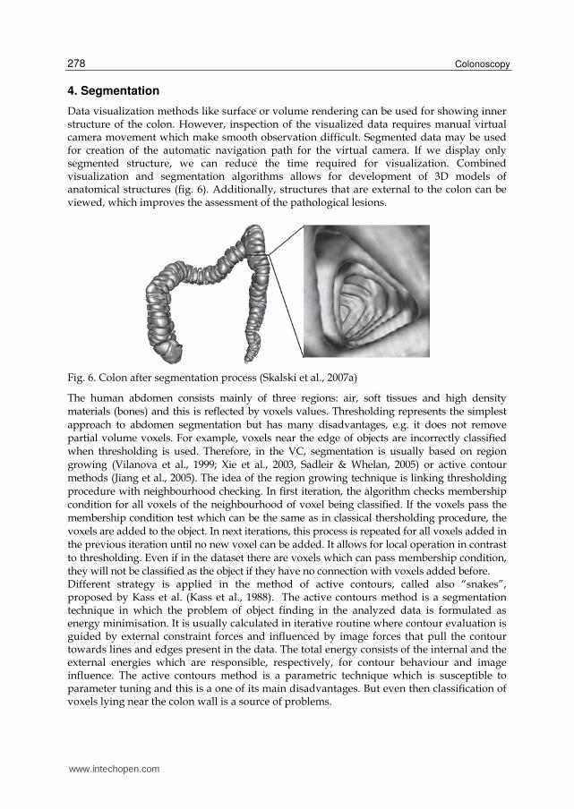
Data visualization methods like surface or volume rendering can be used for showing inner structure of the colon. However, inspection of the visualized data requires manual virtual camera movement which make smooth observation difficult. Segmented data may be used for creation of the automatic navigation path for the virtual camera. If we display only segmented structure, we can reduce the time required for visualization. Combined visualization and segmentation algorithms allows for development of 3D models of anatomical structures (fig. 6). Additionally, structures that are external to the colon can be viewed, which improves the assessment of the pathological lesions.
Fig. 6. Colon after segmentation process (Skalski et al., 2007a)
The human abdomen consists mainly of three regions: air, soft tissues and high density materials (bones) and this is reflected by voxels values. Thresholding represents the simplest approach to abdomen segmentation but has many disadvantages, e.g. it does not remove partial volume voxels. For example, voxels near the edge of objects are incorrectly classified when thresholding is used. Therefore, in the VC, segmentation is usually based on region growing (Vilanova et al., 1999; Xie et al., 2003, Sadleir & Whelan, 2005) or active contour methods (Jiang et al., 2005). The idea of the region growing technique is linking thresholding procedure with neighbourhood checking. In first iteration, the algorithm checks membership condition for all voxels of the neighbourhood of voxel being classified. If the voxels pass the membership condition test which can be the same as in classical thersholding procedure, the voxels are added to the object. In next iterations, this process is repeated for all voxels added in the previous iteration until no new voxel can be added. It allows for local operation in contrast to thresholding. Even if in the dataset there are voxels which can pass membership condition, they will not be classified as the object if they have no connection with voxels added before. Different strategy is applied in the method of active contours, called also “snakes”, proposed by Kass et al. (Kass et al., 1988). The active contours method is a segmentation technique in which the problem of object finding in the analyzed data is formulated as energy minimisation. It is usually calculated in iterative routine where contour evaluation is guided by external constraint forces and influenced by image forces that pull the contour towards lines and edges present in the data. The total energy consists of the internal and the external energies which are responsible, respectively, for contour behaviour and image influence. The active contours method is a parametric technique which is susceptible to parameter tuning and this is a one of its main disadvantages. But even then classification of voxels lying near the colon wall is a source of problems.
www.intechopen.com

Virtual Colonoscopy - Technical Aspects
279
Fig. 7. Idea of the watershed algorithm; First row: classic watershed; Second row: marker-based watershed; description in the text
The 3D segmentation algorithm based on immersion-based watershed method of Vincent
and Soille (Vincent & Soille, 1991) can be also applied. The watershed method exploits
topographic and hydrology concepts for the development of region segmentation methods.
The image may be seen as a topographic relief, in which the value of a pixel (for 2D images)
is interpreted as its altitude in the relief. In case of 2D, the principle of watershed algorithm
can be illustrated by an idea of immersing the image from water sources. When the
neighbouring catchment basins eventually meet, a dam is created to avoid the water spilling
from one basin into the other (Vincent & Soille, 1991). When the water reaches the maximum
value, the edges of the union of all dams form the watershed segmentation results (fig. 7). In
case of 3D, usage of the algorithm leads to receiving 3D objects separated by the dam. If we
use local minima of the image as water sources, oversegmentation problem will appear. In
consequence, we receive a huge number of objects in the resultant matrix which do not
correspond to data.
One of the solutions is a modified strategy of source selection. We used marker-based Watershed transform, where the immersion processes are started from markers computed from the image. In order to improve results, the absolute value of gradient of the filtered data (fig. 8) is computed using the 3D Sobel’s mask and then the data are immersed by the watershed algorithm.
Fig. 8. From left to right: slice of a CT data; Absolute value of the gradient; Gradient visualisation as a topography map
www.intechopen.com

Colonoscopy
280
Neubauer et al. (Neubauer et al., 2002) proposed manual placing of markers inside the data.
On the contrary, we use automatic methods for markers computation: object markers are
obtained from voxels after thresholding operation. We know that voxels having intensity
below 300 units represent air, and background markers are voxels which have intensity
value corresponding to tissues. This approach eliminates the oversegmentation problem.
The 3D watershed segmentation algorithm computes border between the colon and the soft
tissue using the gradient map (fig. 8) calculated as:
2 2 2( , , )MOD x y zG x y z I I I= + + (4)
where Ix, Iy and Iz are image gradients in x, y and z directions, respectively.
Thanks to these operations, the colon model, which is traced, reflects details very precisely
what we can observe in figure 6.
5. Calculation of navigation path
Fast and accurate navigation path generation is essential for efficient diagnosis using the VC
since it allows for simulation of the virtual camera movement inside the segmented
structure and the whole colon can be screened by the physician in a short time. The virtual
camera can be stopped if a suspicious image is discovered for more careful assessment.
Computation of the colon centerline is not a trivial process. The algorithm should require
only minimum operator intervention. Additionally, a centreline approximation of the centre
navigation path of the colon must be obtained in reasonable time with acceptable accuracy.
Time constraint is a very important factor to evaluate the algorithm especially in a clinical
practice.
5.1 State of the art Centreline calculation methods can be subdivided into three categories since they are
mainly based on:
• manual extraction,
• topological thinning (e.g. Xie et al., 2003; Sadleir & Whelan, 2005),
• distance transform (e.g Vilanova et al., 1999). Manual extraction requires manual identification of the centre of colon slices. It does not
guarantee that marked points lie in the centres of slices and that they are directly connected.
Furthermore, the allocation is difficult because the colon centreline is oriented in different
directions.
Methods based on topological thinning and distance transform are automatic usually. The
idea of topological thinning is based on peeling off the colon surface points using
morphological operations repeatedly until the centreline is obtained. Though the results of
this standard algorithm are well-defined they do not always lie in a proper place.
Additionally, the algorithm is extremely inefficient computationally. Therefore, other
methods were developed that use 3D topological thinning and graph search algorithm (Ge
et al. 1999), optimized 3D topological thinning using Look-up Table (Sadleir & Whelan,
2005), distance transform (Zhou & Toga 1999, Van Uitert and Bitter 2007), minimum energy
path (Deschamps and Cohen 2001) or Dijkstra’s shortest path algorithm (Bitter et al. 2000).
www.intechopen.com
Virtual Colonoscopy - Technical Aspects
281
Some approaches rely on the use of the distance transform. In these methods, the centreline is calculated as a maximum of binary mask representing colon after the distance transformation. Below an exemplary algorithm of the VC navigation path calculation is presented.
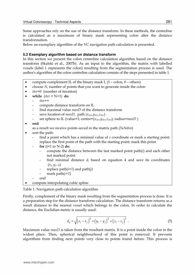
5.2 Exemplary algorithm based on distance transform In this section we present the colon centreline calculation algorithm based on the distance transform (Skalski et al., 2007b). As an input to the algorithm, the matrix with labelled voxels (label L represents the colon) resulting from the segmentation process is used. The author's algorithm of the colon centreline calculation consists of the steps presented in table 1.
• compute complement IL of the binary mask L (1 – colon, 0 – others)
• choose N, number of points that you want to generate inside the colon
• iter=0 (number of iteration)
• while (iter < N+1) do: - iter++ - compute distance transform on IL - find maximal value maxD of the distance transform - save location of maxD, path (xiter,yiter,ziter) - set sphere to IL (value=1; centre=(xiter,yiter,ziter); radius=maxD )
• end
as a result we receive points saved in the matrix path (3xNdim)
• sort the path: - find a point which has a minimal value of z coordinate or mark a starting point;
replace the first point of the path with the starting point; mark this point - for (i=1 to N-2) do:
- compute the distance between the last marked point path(i) and each other not marked point:
- find minimal distance dj based on equation 4 and save its coordinates (xj, yj, zj)
- replace path(i+1) and path(j) - mark path(i+1)
- end
• compute interpolating cubic spline
Table 1. Navigation path calculation algorithm
Firstly, complement of the binary mask resulting from the segmentation process is done. It is a preparation step for the distance transform calculation. The distance transform returns as a result distance to the nearest voxel which belongs to the colon. In order to calculate the distance, the Euclidian metric is usually used:
( ) ( ) ( )2 2 2
= − + − + −ij i j i j i jd x x y y z z . (5)
Maximum value maxD is taken from the resultant matrix. It is a point inside the colon in the widest place. Then, spherical neighbourhood of this point is removed. It prevents algorithms from finding next points very close to points found before. This process is
www.intechopen.com

Colonoscopy
282
repeated in iterative manner. The points received in the previous step become knots of the navigation path. Subsequently, points received from the algorithm are sorted. Finally, points between knots are generated using b-spline cubic interpolation. Exemplary navigation path is presented in figure 9.
Fig. 9. The colon after the segmentation process with a centreline, number of points N = 24
6. Visualisation
The final step in the Virtual Colonoscopy is the data visualization. There are two main
methods of 3D medical data visualization: indirect (surface rendering) and direct (volume
rendering) (Preim & Bartz, 2007). Both techniques can use fully programmable graphical
pipeline.
Surface rendering is one of the indirect methods. This technique produces surfaces in the
domain of the scalar quantity. Scalar values, contained in 3D medical data, represents tissue
properties, like radiodensity in Hounsfield scale or label mask that contains segmentation
results. Surface represents a specific scalar value, the so-called isosurface value. In fact, one
iso-surface describes only one scalar value. The interior of the object is not described –
surface is the boundary of the volume objects. Surface rendering method includes two
stages: generation of the 3D surface from 3D data and proper visualisation relying on the
image generation by graphics accelerator. There are numerous methods for implementing
the surfaces from a discrete set of 3D data (Preim & Bartz, 2007). One of the most useful is
the Marching Cubes algorithm (Lorensen & Cline, 1987). This algorithm has many
implementations that solve the problem of ambiguities in first cell triangulation method
(holes in surface). Possibly the widely used implementation of the Marching Cubes
algorithm comes from The Visualization Toolkit (Schroeder et al., 2004). In the algorithm a
polygonal mesh of the isosurface is generated from the 3D scalar field. The polygonal mesh
is a collection of vertices (points in 3D) connected to triangles. For high resolution data sets
the number of generated graphical primitives can be extremely high. To reduce the number
of triangles, the mesh can be decimated or smoothed (Schroeder et al., 1992 and 2004).
Surface can be coloured according to the isosurface value or to another scalar field using a
texture mapping technique. To increase the perception of the surface shape in the VC
www.intechopen.com

Virtual Colonoscopy - Technical Aspects
283
visualization, the virtual lighting is used. The standard model in the OpenGL Application
Programming Interface is Phong illumination model (Phong, 1975). This is an empirical
model of local illumination. It describes the way a surface reflects the light as a combination
of the diffuse reflection of rough surfaces with the specular reflection of shiny surfaces.
Phong shading includes a model for the reflection of light from surfaces and a compatible
method of estimating pixel colours by interpolating surface normals across rasterized
polygons. In fact, at each point of the screen full Phong model calculations are performed
(per-pixel lighting). Since the interpolation of surface normals is computationally expensive,
the Phong shading is slow. In Gouraud shading algorithm the calculating lighting is
performed only in vertex. Next, the screen pixel colour on the triangle are bilinearly
interpolated from the vertex colour. This method is fast, but the specular highlight will not
be rendered correctly if a highlight lies in the middle of a polygon. This limitation can be
solved by increasing a number of triangles by mesh tessellation or by increasing of spatial
data resolution. The polygonal data can be efficiently processed in modern graphics card.
All shading calculations are done in hardware.
Volume rendering is the process of creating a 2D image directly from 3D volumetric data that operates on the actual data sample without creation of intermediate surfaces consisting of triangles (Preim & Bartz, 2007). The purpose of volume rendering is to effectively convey information present within the volumetric data. It is especially important in case of medical data. All direct volume rendering algorithms can be classified into two main groups: object-space and image-space methods. However, many advanced algorithms cannot by easily classified as one or the other, but fuse aspects from both groups into one hybrid algorithm. Object-space volume rendering techniques use forward mapping scheme where the data is
mapped onto the image plane. One of such approach is the Splatting algorithm that projects
the data voxels onto image-plane (Westover, 1989). Texture-mapping algorithms are the
other widely used object-oriented algorithms. They are supported by computer graphics
hardware. In image-order (image-space) algorithms, a backward mapping scheme is used
where rays are cast from each pixel in the image plane through the volume data to
determine the final pixel colour. The classic direct volume rendering method is the image-
space oriented ray casting algorithm. Moreover, some algorithms use domain-base
techniques – the spatial volume data is first transformed into an alternative domain, such as
frequency or wavelet, and then a projection is generated directly from this domain
(Malzbender, 1993).
Modern graphics cards are characterized by immense ability of 3D data processing. They are
developed and optimized for processing triangle meshes, which are used for surface
rendering. Furthermore, a fully programmable graphics processing unit (GPU) offer new
opportunities to use graphics cards for general purpose computing, especially for volume
rendering. Ray-casting volume rendering using CPUs is computationally expensive since it
requires the interpolation and shading calculations for every sample point along the ray in
the data. Interactive volume ray casting was previously restricted to high-end workstations.
GPU implementations of ray-casting rendering approaches have received great attention
since they enable interactive visualization of volumetric data (Lee et al., 2009).
The most important in virtual colonoscopy visualization is trustworthy surface presentation.
In figure 10, examples of applying different rendering methods are shown. The fastest
method in interactive visualization is the surface rendering. Unfortunately, the triangle
www.intechopen.com

Colonoscopy
284
structure of reconstructed surface has an influence on image quality. The colour
interpolation (diamond artefact) are visible. Surface in image generated by the direct volume
visualization has better quality (fig. 10 b-d). The shape of wrinkles is kept. However, the
computational cost is considerably larger. The texture-mapping technique, supported by the
GPU acceleration, can be used in interactive visualization. Unfortunately, this method
generates images which contain staircase artefacts caused by interpolation and insufficient
depth sampling (fig. 10.d).
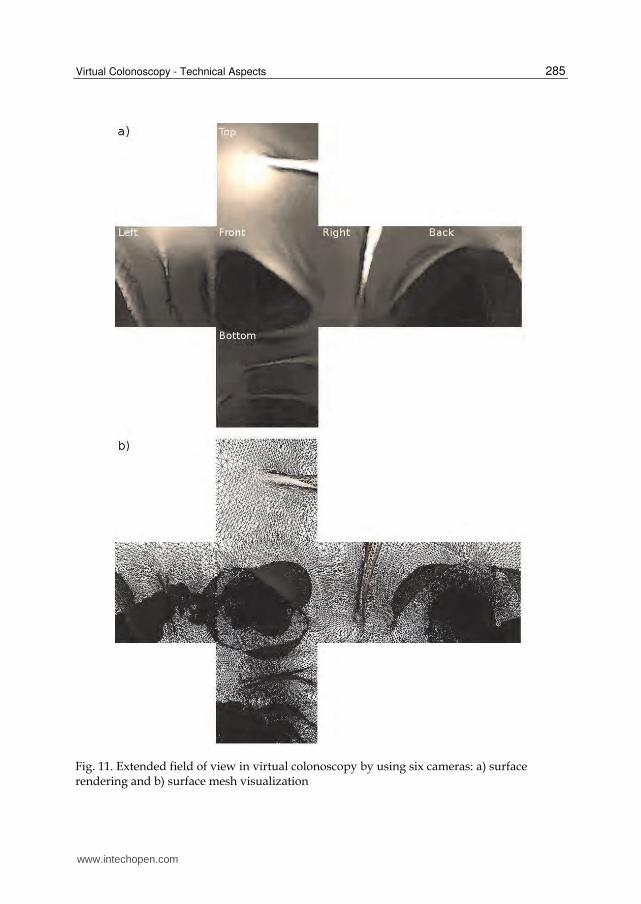
To extend the field of view in virtual colonoscopy the multi-cameras are used, especially for
visual inspection of the colon wall (Serlie I. et al. 2001). The six cameras are located in the
same place, but the view directions are different. They are rotated around, to cover 360
degree of view. Each camera has the 90 degree field of view. Images of this cameras can be
mapped into the unrolled-box surface. The sample of this technique is shown in the figure
11. Additionally, the light source moves along with the camera and the position of light
source is the same as camera position. The light is configured as positional (headlight), and
the cone angle corresponds to camera cone angle. To prevent overexposing nearest surfaces,
the irregular light intensity along the cone angle was used. Light fading attenuation was
used for distance simulation.
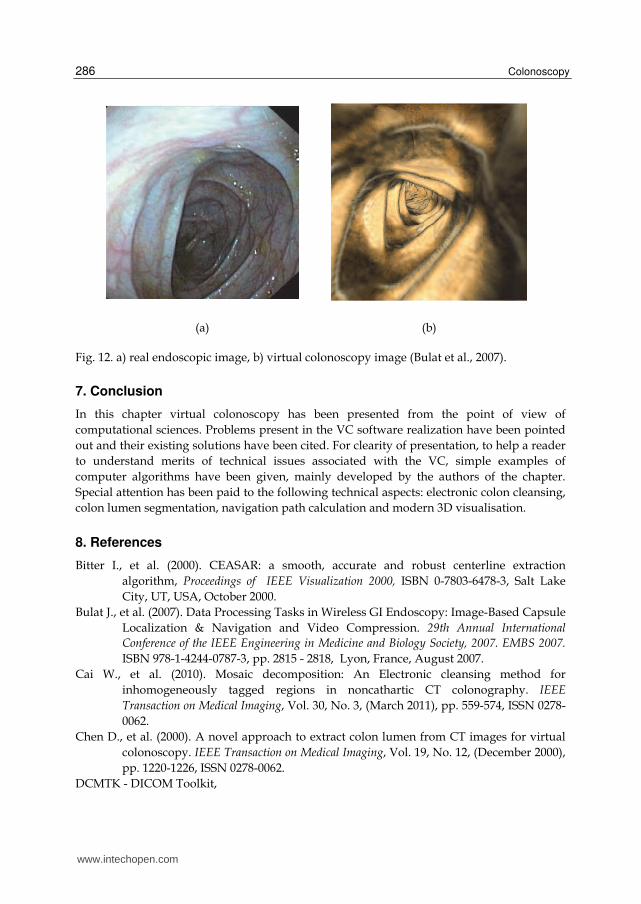
Comparison between real colonoscopic image and virtual one is presented in figure 12.
Fig. 10. Exemplary virtual colonography images: a) surface rendering, b) volume rendering by ray-casting, c) isosurface in volume rendering (ray-casting) and d) texture-mapping volume rendering
www.intechopen.com
Virtual Colonoscopy - Technical Aspects
285
Fig. 11. Extended field of view in virtual colonoscopy by using six cameras: a) surface rendering and b) surface mesh visualization
www.intechopen.com
Colonoscopy
286
(a) (b)
Fig. 12. a) real endoscopic image, b) virtual colonoscopy image (Bulat et al., 2007).
7. Conclusion
In this chapter virtual colonoscopy has been presented from the point of view of
computational sciences. Problems present in the VC software realization have been pointed
out and their existing solutions have been cited. For clearity of presentation, to help a reader
to understand merits of technical issues associated with the VC, simple examples of
computer algorithms have been given, mainly developed by the authors of the chapter.
Special attention has been paid to the following technical aspects: electronic colon cleansing,
colon lumen segmentation, navigation path calculation and modern 3D visualisation.
8. References
Bitter I., et al. (2000). CEASAR: a smooth, accurate and robust centerline extraction
algorithm, Proceedings of IEEE Visualization 2000, ISBN 0-7803-6478-3, Salt Lake
City, UT, USA, October 2000.
Bulat J., et al. (2007). Data Processing Tasks in Wireless GI Endoscopy: Image-Based Capsule
Localization & Navigation and Video Compression. 29th Annual International
Conference of the IEEE Engineering in Medicine and Biology Society, 2007. EMBS 2007.
ISBN 978-1-4244-0787-3, pp. 2815 - 2818, Lyon, France, August 2007.
Cai W., et al. (2010). Mosaic decomposition: An Electronic cleansing method for
inhomogeneously tagged regions in noncathartic CT colonography. IEEE
Transaction on Medical Imaging, Vol. 30, No. 3, (March 2011), pp. 559-574, ISSN 0278-
0062.
Chen D., et al. (2000). A novel approach to extract colon lumen from CT images for virtual
colonoscopy. IEEE Transaction on Medical Imaging, Vol. 19, No. 12, (December 2000),
pp. 1220-1226, ISSN 0278-0062.
DCMTK - DICOM Toolkit,
www.intechopen.com

Virtual Colonoscopy - Technical Aspects
287
http://dicom.offis.de/dcmtk.php.en, accessed on April 2, 2011
Deschamps T. & Cohen L. D. (2001). Fast extraction of minimal paths in 3-D images and
applications to virtual endoscopy Medical Image Analysis, Vol. 5, No. 4, (December
2001) pp. 281 - 289, ISSN 1361-8415.
DICOM - Digital Imaging and Communications in Medicine, http://medical.nema.org/,
accessed on April 1, 2011
Florie J., et al. (2007). MR colonography with limited bowel preparation compared with
optical colonoscopy in patients at increased risk for colorectal cancer. Radiology.
Vol. 243, No. 1, (December 2007), pp. 122-131, ISSN 1527-1315.
Frentz S.M. & Summers R.M. (2006). Current Status of CT Colonography. Academic
Radiology, Vol. 13, No. 12, (December 2006), pp. 1517-1531, ISSN: 1076-6332.
GDCM - Grassroots DICOM library, http://sourceforge.net/apps/mediawiki/gdcm, accessed on
March 25, 2011.
Ge Y., et al. (1999). Computing the centerline of a colon: a robust and efficient method based
on 3D skeletons, Journal of Computer Assisted Tomography. Vol. 23, No. 5,
(September- October 1999) pp. 786–794, ISSN 0363-8715
Graser A., et al. (2009). Comparison of CT colonography, colonoscopy, sigmoidoscopy and
fecal occult blood tests for the detection of advanced adenomas in an average risk
population. Gut, Vol. 58, No. 2, ( October 2008), pp. 241-248, ISSN 1468-3288.
Hong L. et al. (1996). Visible Human Virtual Colonoscopy. Conference of National Library of
Medicine Visible Human Project, pp. 29-30, October 1996.
Hong L. et al. (1997). Virtual Voyage: Interactive Navigation in the Human Colon.
Proceedings of the 24th annual conference on Computer graphics and interactive
techniques, ACM SIGGRAPH’97, ISBN:0-89791-896-7, pp. 27-34, August 1997.
Iannaccone R., et al. (2004). Computed tomography colonography without cathartic
preparation for the detection of colorectal polyps. Gastroenterology, Vol. 127, No. 5,
(November 2004), pp. 1300-1311, ISSN 0016-5085.
Jiang R.; Berliner L. & Meng J (2005). Computer graphics enhancements in CT Colography
for improved diagnosis and navigation. International Congress Series: CARS 2005:
Computer Assisted Radiology and Surgery, Vol. 1281, ISSN 0531-5131, pp. 109-114.
May 2005.
Kak A. C. & Slaney M. (1988). Principles of Computerized Tomographic Imaging. IEEE
Press, ISBN 0-87942-198-3, New York, NY, USA, also available from
http://www.slaney.org/pct/pct-toc.html.
Kass M., Witkin A &, Terzopoulos D. (1988). Snakes: Active contour models. International
Journal on Computer Vision, Vol. 1, No. 4, (January 1988), pp. 321-331, ISSN 1573-
1405.
Lakare S., et al. (2002). Electronic Colon Cleansing using Segmentation Rays for Virtual
Colonoscopy. Proceedings of SPIE Medical Imaging - Physiology and Function from
Multidimensional Images. Vol. 4683, ISBN 9-78081944-428-8, pp. 412-418, April 2002.
Lakare S., et al. (2003). Robust colon residue detection using vector quantization based
classification for virtual colonoscopy. Proceedings of SPIE, Medical Imaging 2003:
Physiology and Function: Methods, Systems, and Applications, Vol. 5031, ISBN 9-
78081944-832-3 ,pp. 515-520, May 2003.
www.intechopen.com

Colonoscopy
288
Levin B., et al. (2008). Screening and surveillance for the early detection of colorectal cancer
and adenomatous polypos, 2008: a joint guideline from the American Cancer
Society, the US Multi-Society Task Force on Colorectal Cancer, and the American
College of Radiology. Gastroenterology Vol. 134, No. 5, (May 2008), pp. 1570-1595,
ISSN 1528-0012.
Lee T.-H., et al. (2009) Fast perspective volume ray casting method using GPU-based
acceleration techniques for translucency rendering in 3D endoluminal CT
colonography, Computers in Biology and Medicine, Vol. 39, No. 8, (August 2009), pp.
657-666, ISSN 1879-0534.
Lorensen W.E. & Cline H.E. (1987). Marching Cubes: A high resolution 3D surface
construction algorithm. ACM SIGGRAPH Computer Graphics, Vol. 21, No. 4, (July
1987), pp. 163-169, ISSN:0097-8930.
Malzbender T. (1993). Fourier volume rendering. ACM Transactions on Graphics Vol. 12, No.
3, (July 1993), pp. 233–250, ISSN:0730-0301.
Neubauer A., et al. (2002). Fast and Flexible Iso-Surfacing for Virtual Endoscopy. Proceedings
of the sixth Central European Seminar on Computer Graphics CESCG. Budmerice,
Slovakia, April 22-24, 2002,
http://old.vrvis.at/TR/2002/TR_VRVis_2002_013_Full.pdf
Pickhardt P.J.; Taylor A.J. & Gopal D.V. (2006). Surface Visualization at 3D Endoluminac CT
Colonography: Degree of Coverage and Implications for Polyp Detection.
Gastroenterology. Vol. 130, No. 6 (May 2006) pp. 1582-1587, ISSN 0016-5085.
Phong B.-T. (1975). Illumination for computer generated pictures. Communications of ACM
Vol. 18, No. 6, (June 1975), pp. 311–317, ISSN 0001-0782.
Preim B. & Bartz D. (2007). Visualization in Medicine: Theory, Algorithms, and Applications
(The Morgan Kaufmann Series in Computer Graphics). (1 ed.) Morgan Kaufmann
Publishers Inc., ISBN 9-78012370-596-9, San Francisco, CA, USA.
Regge D., et al. (2009). Diagnostic accuracy of computed tomographic colonography for the
detection of advance neoplasia in individuals at increased risk of colorectal cancer.
JAMA, Vol. 301, No. 23, (June 2009), pp. 2453-2461, ISSN 1538-3598.
Sadleir R. & Whelan P. (2005). Fast colon centreline calculation using optimised 3D
topological thinning. Computerized Medical Imaging and Graphics. Vol. 29, No. 4,
(December 2004), pp. 251-258, ISSN 0895-6111.
Schroeder W., Zarge J., & Lorensen W. (1992). Decimation of triangle meshes, ACM
SIGGRAPH Computer Graphics, Vol. 26, No. 2, (July 1992), pp.65-70, ISSN 0097-8930.
Schroeder W., Martin K. & Lorensen B. (2006). Visualization Toolkit: An Object-Oriented
Approach to 3D Graphics. (4th ed.) Kitware, ISBN 1-930934-19-X .
Serlie I, et al. (2001). Maximizing Surface Visibility in Virtual Colonoscopy. ASCI 2001
Proceedings of the Seventh Annual Conference of Advanced School for Computing and
Imaging. ISBN 90-803086-6-8, Heijen, The Netherlands, pp. 196-201, May/June 2001.
Serlie I, et al. (2010). Electronic cleansing for computed tomography (CT) colonography
using a scale-invariant three-material model. IEEE Transactions on Biomedical
Engineering, Vol. 57, No. 6, (June 2010), pp. 1306-1317, ISSN 0018-9294.
www.intechopen.com
Virtual Colonoscopy - Technical Aspects
289
Sezille N.; Sadleir R. & Whelan P.F. (2003). Automated synthesis, insertion and detection of
polyps for CT colonography. Opto-Ireland 2002, Proceedings of the SPIE, Vol. 4877,
ISBN 9-78081944-658-9, Galway, Ireland, pp. 183-191, September 2002.
Skalski A., et al. (2007a). Colon cleansing for virtual colonoscopy using non-linear transfer
function and morphological operations. Proceedings of the 2007 IEEE international
workshop on Imaging systems and techniques. ISBN 1-4244-0965-9, Krakow, Poland,
pp. 1-5, May 2007.
Skalski A., et al. (2007b). CT data processing and visualization aspects of virtual
colonoscopy. EUSIPCO 2007, 15th European signal processing conference, ISBN 978-83-
921340-2-2, Poznań, Poland, pp. 2509–2513, September 2007.
Summers R, et al. (2005). Computer-aided detection of polyps on oral contrast-enhanced CT
colonography. American Journal Roentgenology, Vol. 184, No. 1, (January 2005) pp.
105-108, ISSN 0361-803X.
The Visible Human Project. U.S. National Library of Medicine
http://www.nlm.nih.gov/research/visible/visible_human.html, accessed on April 2, 2011.
Wang Z., et al. (2006). An improved electronic colon cleansing method for detection of
colonic polyps by virtual colonoscopy. IEEE Transaction on Biomedical Engineering,
Vol. 53, No. 8, (August 2006), pp. 1635-1646, ISSN 0018-9294.
Wang J., et al. (2008). Virtual Colonoscopy Screening With Ultra Low-Dose CT and Less-
Stressful Bowel Preparation: A Computer Simulation Study. IEEE Transactions on
Nuclear Science, Vol. 55, No.5, (October 2008), pp. 2566-2575, ISSN 0018-9499.
Wax M., et al. (1998). Electronic colon cleansing for virtual colonoscopy. Proc. 1st Symposium
on Virtual Colonoscopy, Boston, USA, pp. 94-94, 1998.
Van Uitert R.L. & Bitter I., (2007). Subvoxel precise skeletons of volumetric data based on
fast marching methods, Medical Physics, Vol. 34, No. 2, (January 2007), pp. 627–638,
ISSN 0094-2405.
Van Uitert R.L. et al. (2008). Temporal and multiinstitutional quality assessment of CT
Colonography. American Journal of Roentegenology Vol. 191, No. 5, (November 2008)
pp. 1503-1504, ISSN 1546-3141.
Vilanova A.; König A & Gröller E. (1999). VirEn: A Virtual Endoscopy System. Machine
Graphics & Vision. Vol. 8 No. 3, (1999),pp. 469-487, ISSN 1230-0535.
Vincent L. & Soille P. (1991). Watersheds in digital spaces: An efficient algorithm based on
immersion simulations. IEEE Transactions on Pattern Analysis and Machine
Intelligence. Vol. 13, No. 6, ( June 1991), pp. 583-598, ISSN 0162-8828.
VTK – Visualzation Toolkit, http://www.vtk.org, accessed on April 2, 2011.
Xie W.; Thompson R.P. & Perucchio R. (2003). A topology-preserving parallel 3D thinning
algorithm for extracting the curve skeleton. Pattern Recognition, Vol. 36, No. 7, (July
2003), pp. 1529-1544, ISSN 0031-3203.
Yoshida H. et al. (2002) . Computer-aided Diagnosis Scheme for Detection of Polyps at CT
Colonography. Radiographics, Vol. 22, No. 4, (July/August 2002), pp. 963- 979. ISSN
0271-5333.
Zalis M.E., Perumpillichira J. & Hahn P.F. (2004). Digital substraction bowel cleansing for
CT colonography using morphological and linear filtration methods. IEEE
www.intechopen.com

Colonoscopy
290
Transactions on Medical Imaging, Vol. 23, No. 11, (November 2004), pp. 1335-1343,
ISSN 0278-0062.
Zhou Y. & Toga A.W., (1999). Efficient skeletonization of volumetric objects. IEEE
Transactions on Visualization and Computer Graphics,, Vol. 5, No. 3, (July - September
1999) pp. 196–209, ISSN 1077-2626.
www.intechopen.com

ColonoscopyEdited by Prof. Paul Miskovitz
ISBN 978-953-307-568-6Hard cover, 326 pagesPublisher InTechPublished online 29, August, 2011Published in print edition August, 2011
InTech EuropeUniversity Campus STeP Ri Slavka Krautzeka 83/A 51000 Rijeka, Croatia Phone: +385 (51) 770 447 Fax: +385 (51) 686 166www.intechopen.com
InTech ChinaUnit 405, Office Block, Hotel Equatorial Shanghai No.65, Yan An Road (West), Shanghai, 200040, China
Phone: +86-21-62489820 Fax: +86-21-62489821
To publish a book on colonoscopy suitable for an international medical audience, drawing upon the expertiseand talents of many outstanding world-wide clinicians, is a daunting task. New developments invideocolonoscope instruments, procedural technique, patient selection and preparation, and moderatesedation and monitoring are being made and reported daily in both the medical and the lay press. Just as overthe last several decades colonoscopy has largely supplanted the use of barium enema x-ray study of thecolon, new developments in gastrointestinal imaging such as computerized tomographic colonography andvideo transmitted capsule study of the colonic lumen and new discoveries in cellular and molecular biology thatmay facilitate the early detection of colon cancer, colon polyps and other gastrointestinal pathology threaten torelegate the role of screening colonoscopy to the side lines of medical practice. This book draws on the talentsof renowned physicians who convey a sense of the history, the present state-of-the art and ongoingconfronting issues, and the predicted future of this discipline.
How to referenceIn order to correctly reference this scholarly work, feel free to copy and paste the following:
Andrzej Skalski, Mirosław Socha, Tomasz Zielin ́ski and Mariusz Duplaga (2011). Virtual Colonoscopy -Technical Aspects, Colonoscopy, Prof. Paul Miskovitz (Ed.), ISBN: 978-953-307-568-6, InTech, Available from:http://www.intechopen.com/books/colonoscopy/virtual-colonoscopy-technical-aspects

© 2011 The Author(s). Licensee IntechOpen. This chapter is distributedunder the terms of the Creative Commons Attribution-NonCommercial-ShareAlike-3.0 License, which permits use, distribution and reproduction fornon-commercial purposes, provided the original is properly cited andderivative works building on this content are distributed under the samelicense.