STATISTICALINFERENCE

Vijay K. RohatgiProfessor Emeritus

Bowling Green State University

Dover Publications, Inc.Mineola, New York

To Bina and Sameer

CopyrightCopyright © 1984, 2003 by Vijay K. RohatgiAll rights reserved.

Bibliographical NoteThis Dover edition, first published in 2003, is an unabridged reprint of the work published by John Wiley & Sons, New York, 1984. An errata

list has been specially prepared for this edition.

Library of Congress Cataloging-in-Publication DataRohatgi, V.K., 1939–

Statistical inference / Vijay K. Rohatgi.p. cm.

Originally published: New York : Wiley, c1984, in series in probability and mathematical statistics. Probability and mathematicalstatistics.

Includes index.ISBN 0-486-42812-5 (pbk.)

1. Mathematical statistics. I. Title.

QA276.R624 2003519.5—dc21

2003046063

Manufactured in the United States of AmericaDover Publications, Inc., 31 East 2nd Street, Mineola, N.Y. 11501

PREFACE

This course in statistical inference is designed for juniors and seniors in most disciplines (includingmathematics). No prior knowledge of probability or statistics is assumed or required. For a class meetingfour hours a week this is a two-semester or three-quarter course. The mathematical prerequisite ismodest. The prospective student is expected to have had a three-semester or four-quarter course incalculus. Whenever it is felt that a certain topic is not covered in a calculus course at the statedprerequisite level, enough supplementary details are provided. For example, a section on gamma and betafunctions is included, as are supplementary details on generating functions.

There are many fine books available at this level. Then why another? Their titles notwithstanding,almost all of these books are in probability and statistics. Roughly the first half of these texts is usuallydevoted to probability and the second half to statistics. Statistics almost always means parametricstatistics, with a discussion of nonparametric statistics usually relegated to the last chapter.

This text is on statistical inference. My approach to the subject separates this text from the rest inseveral respects. First, probability is treated here from a modeling viewpoint with strong emphasis onapplications. Second, statistics is not relegated to the second half of the course—indeed, statisticalthinking is encouraged and emphasized from the beginning. Formal language of statistical inference isintroduced as early as Chapter 4 (essentially the third chapter, since Chapter 1 is introductory),immediately after probability distributions have been introduced. Inferential questions are consideredalong with probabilistic models, in Chapters 6 and 7. This approach allows and facilitates an earlyintroduction to parametric as well as nonparametric techniques. Indeed, every attempt has been made tointegrate the two: Empirical distribution function is introduced in Chapter 4, in Chapter 5 we show that itis unbiased and consistent, and in Chapter 10 we show that it is the maximum likelihood estimate of thepopulation distribution function. Sign test and Fisher–Irwin test are introduced in Chapter 6, and inferenceconcerning quantiles is covered in Section 8.5. There is not even a separate chapter entitlednonparametric statistical inference.

Apart from the growing importance of and interest in statistics, there are several reasons forintroducing statistics early in the text. The traditional approach in which statistics follows probabilityleaves the reader with the false notion that probability and statistics are the same and that statistics is themathematics of computing certain probabilities. I do not believe that an appreciation for the utility ofstatistics should be withheld until a large dose of probability is digested. In a traditional course, studentswho leave the course after one semester or one quarter learn little or no statistics. They are left with littleunderstanding of the important role that statistics plays in scientific research. A short course inprobability becomes just another hurdle to pass before graduation, and the students are deprived of thechance to use statistics in their disciplines. I believe that the design of this text alleviates these problemsand enables the student to acquire an outlook approaching that of a modern mathematical statistician andan ability to apply statistical methods in a variety of situations.

There appears to be a reasonable agreement on the topics to be included in a course at this level. Idepart a little from the traditional coverage, choosing to exclude regression since it did not quite fit intothe scheme of “one sample, two sample, many sample” problems. On the other hand, I include theFriedman test, Kendall’s coefficient of concordance, and multiple comparison procedures, which areusually not done at this level.

The guiding principles in my selection have been usefulness, interrelationship, and continuity. Theordering of the selections is dictated by need rather than relative importance.

While the topics covered here are traditional, their order, coverage, and discussion are not. Manyother features of this text separate it from previous texts. I mention a few here:

(i)

An unusually large number of problems (about 1450) and examples (about 400) are included.Problems are included at the end of each section and are graded according to their degree ofdifficulty; more advanced (and usually more mathematical) problems are identified by anasterisk. A set of review problems is also provided at the end of each chapter to test thestudent’s ability to choose relevant techniques. Every attempt has been made to avoid theannoying and time-consuming practice of creating new problems by referring to earlierproblems (often scores of pages earlier). Either completely independent problems are given ineach section or relevant details (with cross references) are restated whenever a problem isimportant enough to be continued in a later section. The amount of duplication, however, isminimal and improves readability.

(ii)

Sections with a significant amount of mathematical content are also identified by an asterisk.These sections are aimed at the more mathematically inclined students and may be omitted atfirst reading. This procedure allows us to encompass a much wider audience withoutsacrificing mathematical rigor. Needless to say, this is not a recipe book. The emphasis is onthe how and why of all the techniques introduced here, in the hope that the student ischallenged to think like a statistician.

(iii)

Applications are included from diverse disciplines. Most examples and problems areapplication oriented. It is true that no attempt has been made to include “real life data” in theseproblems and examples but I hope that the student will be motivated enough to follow up thiscourse with an exploratory data analysis course.

(iv) A large number of figures (about 150) and remarks supplement the text. Summaries of mainresults are highlighted in boxed or tabular form.

In a two-semester course, meeting four times a week, my students have been able to cover the firsttwelve chapters of the text without much haste. In the first semester we cover the first five chapters with agreat deal of emphasis on Chapter 4, the introduction to statistical inference. In the second semester wecover all of Chapters 6 and 7 on models (but at increased pace and with emphasis on inferentialtechniques), most of Chapter 8 on random variables and random vectors (usually excluding Section 6,depending on the class composition), and all of Chapter 9 on large-sample theory.

In Chapter 10 on point and interval estimation, more time is spent on sections on sufficiency, methodof moments, maximum likelihood estimation, and confidence intervals than on other sections. In Chapter11 on testing hypotheses, we emphasize sections on Wilcoxon signed rank test, two-sample tests, chi-square test of goodness of fit, and measures of association. The point is that if the introductory chapter onstatistical inference (Chapter 4) is covered carefully, then one need not spend much time on unbiasedestimation (Section 10.3), Neyman- Pearson Lemma (Section 11.2), composite hypotheses (Section 11.3),or likelihood ratio tests (Section 11.4). Chapter 12 on categorical data is covered completely.

In a three-quarters course, the pace should be such that the first four chapters are covered in the firstquarter, Chapters 5 to 9 in the second quarter, and the remaining chapters in the third quarter. If it is foundnecessary to cover Chapter 13 on k-sample problems in detail, we exclude the technical sections ontransformations (Section 8.3) and generating functions (Section 8.6), and also sections on inferenceconcerning quantiles (Section 9.8), Bayesian estimation (Section 10.6), and composite hypotheses(Section 11.3).

I take this opportunity to thank many colleagues, friends, and students who made suggestions forimprovement. In particular, I am indebted to Dr. Humphrey Fong for drawing many diagrams, to Dr.Victor Norton for some numerical computations used in Chapter 4 and to my students, especially LisaKillel and Barbara Christman, for checking many solutions to problems. I am grateful to the Literary

Executor of the late Sir Ronald A. Fisher, F. R. S., to Dr. Frank Yates, F. R. S., and to Longman GroupLtd., London, for permission to reprint Tables 3 and 4 from their book Statistical Tables for Biological ,Agricultural and Medical Research (6th edition, 1974). Thanks are also due to Macmillan PublishingCompany, Harvard University Press, the Rand Corporation, Bell Laboratories, Iowa University Press,John Wiley & Sons, the Institute of Mathematical Statistics, Stanford University Press, WadsworthPublishing Company, Biometrika Trustees, Statistica Neerlandica, Addison–Wesley Publishing Company,and the American Statistical Association for permission to use tables and to John Wiley & Sons forpermission to use some diagrams.

I also thank the several anonymous reviewers whose constructive comments greatly improvedpresentation. Finally, I thank Mary Chambers for her excellent typing and Beatrice Shube, my editor atJohn Wiley & Sons, for her cooperation and support in this venture.

VIJAY K. ROHATGI

Bowling Green, OhioFebruary 1984

CONTENTS

CHAPTER 1. INTRODUCTION

1.1 Introduction1.2 Stochastic Models1.3 Probability, Statistics, and Inference

CHAPTER 2. PROBABILITY MODEL

2.1 Introduction2.2 Sample Space and Events2.3 Probability Axioms2.4 Elementary Consequences of Axioms2.5 Counting Methods2.6 Conditional Probability2.7 Independence2.8 Simple Random Sampling from a Finite Population2.9 Review Problems

CHAPTER 3. PROBABILITY DISTRIBUTIONS

3.1 Introduction3.2 Random Variables and Random Vectors3.3 Describing a Random Variable3.4 Multivariate Distributions3.5 Marginal and Conditional Distributions3.6 Independent Random Variables3.7 Numerical Characteristics of a Distribution—Expected Value3.8 Random Sampling from a Probability Distribution3.9 Review Problems

CHAPTER 4. INTRODUCTION TO STATISTICAL INFERENCE

4.1 Introduction4.2 Parametric and Nonparametric Families4.3 Point and Interval Estimation4.4 Testing Hypotheses4.5 Fitting the Underlying Distribution4.6 Review Problems

CHAPTER 5. MORE ON MATHEMATICAL EXPECTATION

5.1 Introduction5.2 Moments in the Multivariate Case5.3 Linear Combinations of Random Variables5.4 The Law of Large Numbers5.5* Conditional Expectation5.6 Review Problems

CHAPTER 6. SOME DISCRETE MODELS

6.1 Introduction6.2 Discrete Uniform Distribution6.3 Bernoulli and Binomial Distributions6.4 Hypergeometric Distribution6.5 Geometric and Negative Binomial Distributions: Discrete Waiting-Time Distribution6.6 Poisson Distribution6.7 Multivariate Hypergeometric and Multinomial Distributions6.8 Review Problems

CHAPTER 7. SOME CONTINUOUS MODELS

7.1 Introduction7.2 Uniform Distribution7.3* Gamma and Beta Functions7.4 Exponential, Gamma, and Weibull Distributions7.5* Beta Distribution7.6 Normal Distribution7.7* Bivariate Normal Distribution7.8 Review Problems

CHAPTER 8. FUNCTIONS OF RANDOM VARIABLES AND RANDOM VECTORS

8.1 Introduction8.2 The Method of Distribution Functions?8.3* The Method of Transformations8.4 Distributions of Sum, Product, and Quotient of Two Random Variables8.5 Order Statistics8.6* Generating Functions8.7 Sampling From a Normal Population8.8 Review Problems

CHAPTER 9. LARGE-SAMPLE THEORY

9.1 Introduction9.2 Approximating Distributions: Limiting Moment Generating Function9.3 The Central Limit Theorem of Lévy9.4 The Normal Approximation to Binomial, Poisson, and Other Integer-Valued Random

Variables

9.5 Consistency9.6 Large-Sample Point and Interval Estimation9.7 Large-Sample Hypothesis Testing9.8 Inference Concerning Quantiles9.9 Goodness of Fit for Multinomial Distribution: Prespecified Cell Probabilities9.10 Review Problems

CHAPTER 10. GENERAL METHODS OF POINT AND INTERVAL ESTIMATION

10.1 Introduction10.2 Sufficiency10.3 Unbiased Estimation10.4 The Substitution Principle (The Method of Moments)10.5 Maximum Likelihood Estimation10.6* Bayesian Estimation10.7 Confidence Intervals10.8 Review Problems

CHAPTER 11. TESTING HYPOTHESES

11.1 Introduction11.2 Neyman–Pearson Lemma11.3* Composite Hypotheses11.4* Likelihood Ratio Tests11.5 The Wilcoxon Signed Rank Test11.6 Some Two-Sample Tests11.7 Chi-Square Test of Goodness of Fit Revisited11. 8* Kolmogorov-Smirnov Goodness of Fit Test11.9 Measures of Association for Bivariate Data11.10 Review Problems

CHAPTER 12. ANALYSIS OF CATEGORICAL DATA

12.1 Introduction12.2 Chi-Square Test for Homogeneity12.3 Testing Independence in Contingency Tables12.4 Review Problems

CHAPTER 13. ANALYSIS OF VARIANCE: k-SAMPLE PROBLEMS

13.1 Introduction13.2 One-Way Analysis of Variance13.3 Multiple Comparison of Means13.4 Two-Way Analysis of Variance13.5 Testing Equality in k-Independent Samples: Nonnormal Case13.6 The Friedman Test for k-Related Samples13.7 Review Problems

APPENDIX—TABLES

ANSWERS TO ODD-NUMBERED PROBLEMS

INDEX

ERRATA

CHAPTER 1

Introduction

1.1 INTRODUCTION

Probabilistic statements are an integral part of our language. We use the expressions random, odds,chance, risk, likelihood, likely, plausible, credible, as likely as not, more often than not, almost certain,possible but not probable, and so on. All these words and phrases are used to convey a certain degree ofuncertainty although their nontechnical usage does not permit sharp distinctions, say, between probableand likely or between improbable and impossible. One of our objectives in this course is to introduce (inChapter 2) a numerical measure of uncertainty. Once this is done we can use the apparatus of mathematicsto describe many physical or artificial phenomena involving uncertainty. In the process, we shall learn touse some of these words and phrases as technical terms.

The basic objective of this course, however, is to introduce techniques of statistical inference. It ishardly necessary to emphasize here the importance of statistics in today’s world. Statistics is used inalmost every field of activity. News media carry statistics on unemployment rate, inflation rate, battingaverages, average rainfall, the money supply, crime rates. They carry the results of Gallop and Harrispolls and many other polls. Most people associate statistics with a mass of numerical facts, or data. Tobe sure statistics does deal with the collection and description of data. But a statistician does much more.He or she is—or should be—involved in the planning and design of experiments, in collectinginformation, and in deciding how best to use the collected information to provide a basis for decisionmaking. This text deals mostly with this latter aspect: the art of evaluating information to draw reliableinferences about the true nature of the phenomenon under study. This is called statistical inference.

1.2 STOCHASTIC MODELS

Frequently the objective of scientific research is to give an adequate mathematical description of somenatural or artificial phenomenon. A model may be defined as a mathematical idealization used toapproximate an observable phenomenon. In any such idealization, certain assumptions are made (andhence certain details are ignored as unimportant). The success of the model depends on whether or notthese assumptions are valid (and on whether the details ignored actually are unimportant).

In order to check the validity of a model, that is, whether or not a model adequately describes thephenomenon being studied, we take observations. The process of taking observations (to discoversomething that is new or to demonstrate something that is already known) is called an experiment.

A deterministic model is one which stipulates that the conditions under which an experiment isperformed determine the outcome of the experiment. Thus the distance d traveled by an automobile in timet hours at a constant speed s kilometers per hour is governed by the relation d = st. Knowledge of s and tprecisely determines d. Similarly, gravitational laws describe precisely what happens to a falling object,and Kepler’s laws describe the behavior of planets.

A nondeterministic (or stochastic) model, on the other hand, is one in which past information, nomatter how voluminous, does not permit the formulation of a rule to determine the precise outcome of an

experiment. Many natural or artificial phenomena are random in the sense that the exact outcome cannotbe predicted, and yet there is a predictable long-term pattern. Stochastic models may be used to describesuch phenomena. Consider, for example, the sexes of newborns in a certain County Hospital. Let B denotea boy and G a girl. Suppose sexes are recorded in order of birth. Then we observe a sequence of letters Band G, such as

GBGGBGBBBGG… .

This sequence exhibits no apparent regularity. Moreover, one cannot predict the sex of the next newborn,and yet one can predict that in the long run the proportion of girls (or boys) in this sequence will settledown near 1/2. This long-run behavior is called statistical regularity and is noticeable, for example, inall games of chance.

In this text we are interested only in experiments that exhibit the phenomena of randomness andstatistical regularity. Probability models are used to describe such phenomena.

We consider some examples.

Example 1. Measuring Gravity. Consider a simple pendulum with unit mass suspended from a fixed point O which swings onlyunder the effect of gravity. Assume that the string is of unit length and is weightless. Let t = t(θ) be the period of oscillation when θ is theangle between the pendulum and the vertical (see Figure 1). It is shown in calculus† that when the pendulum goes from θ = θ0 to θ = 0(corresponding to one fourth of a period)

Figure 1

so that

Hence for small oscillations k = 0 and gives approximately the period of oscillation. This gives a deterministic modelgiving g as a function of t, namely,

If t can be measured accurately, this formula gives the value of g. If repeated readings on t are taken, they will all be found different(randomness) and yet there will be a long-run pattern in that these readings will all concentrate near the true value of t (statisticalregularity). The randomness may be due to limitations of our measuring device and the ability of the person taking the readings. To takeinto account these nondeterministic factors we may assume that t varies in some random manner such that

where is the true value of t and ε is a random error that varies from reading to reading. A stochastic model will postulate that

along with some assumptions about the random error ε. A statistician’s job, then, is to estimate g based on, say, nreadings t1, t2, …, tn on t.

Example 2. Ohm’s Law. According to Ohm’s law for a simple circuit, the voltage V is related to the current I and the resistance Raccording to the formula V = IR. If the conditions underlying this deterministic relationship are met, this model predicts precisely the valueof V given those of I and R. Such a description may be adequate for most practical purposes.

If, on the other hand, repeated readings of either I or R or both are found to vary, then V will also vary in a random manner. Given apair of readings on I and R, V is still determined by V = IR. Since all pairs of readings on I and R are different, so will be the values of V.In a stochastic model the assumptions we make concerning the randomness in I and/or R determine the random behavior of V through therelation V = IR.

Example 3. Radioactive Disintegration. The deterministic model for radioactive disintegration postulates that the rate of decay of aquantity of radioactive element is proportional to the mass of the element. That is,

where λ > 0 is a constant giving the rate of decay and m is the mass of the element. Integrating (1) with respect to t we get:

where c is a constant. If m = m0 at time t = 0, then c = In m0 and we have:

for t ≤ 0. Given m0 and λ, we know m as a function of t.The exact number of decays in a given time interval, however, cannot be predicted with certainty because of the random nature of the

time at which an element disintegrates. This forces us to consider a stochastic model. In a stochastic model one makes certainassumptions concerning the probability that a given element will decay in time interval [0, t]. These lead to an adequate description of theprobability of exactly k decays in [0, t].

Example 4. Rolling a Die. A die is rolled. Let X be the number of points (face value) on the upper face. No deterministic model canpredict which of the six face values 1, 2, 3, 4, 5, or 6 will show up on any particular roll of the die (randomness) and yet there is apredictable long-run pattern. The proportion of any particular face value in a sequence of rolls will be about provided the die is notloaded.

It should be clear by now that in some experiments a deterministic model is adequate. In otherexperiments (Examples 3 and 4) we must use a stochastic model. In still other experiments, a stochasticmodel may be more appropriate than a deterministic model. Experiments for which a stochastic model ismore appropriate are called statistical or random experiments.

DEFINITION 1. (RANDOM OR STATISTICAL EXPERIMENT). An experiment that has the followingfeatures is called a random or statistical experiment.

(i) All possible outcomes of the experiment are known in advance.(ii) The exact outcome of any specific performance of the experiment is unpredictable

(randomness).(iii) The experiment can be repeated under (more or less) identical conditions.(iv) There is a predictable long-run pattern (statistical regularity).

Example 5. Some Typical Random Experiments. We list here some typical examples of random experiments.

(i) Toss a coin and observe the up face.(ii) A light bulb manufactured at a certain plant is put to a lifetime test and the time at which it fails

is recorded.(iii) A pair of dice is rolled and the face values that show up are recorded.(iv) A lot consisting of N items containing D defectives (D ≤ N) is sampled. An item sampled is not

replaced, and we record whether the item selected is defective or nondefective. The processcontinues until all defective items are found.

(v) The three components of velocity of an orbital satellite are recorded continuously for a 24-hourperiod.

(vi) A manufacturer of refrigerators inspects its refrigerators for 10 types of defects. The number ofdefects found in each refrigerator inspected is recorded.

(vii) The number of girls in every family with five children is recorded for a certain town.

Problems for Section 1.2

In the following problems, state whether a deterministic or a nondeterministic model is more appropriate.Identify the sources of randomness. (In each case there is no clearly right or wrong answer; the decisionyou make is subjective.)

1. The time (in seconds) elapsed is measured between the end of a question asked of a person and thestart of her or his response.

2. In order to estimate the average size of a car pool, a selection of cars is stopped on a suburban highwayand the number of riders recorded.

3. On a graph paper, a line with equation y = 3x + 5 is drawn and the values of y for x = 1, 3, 5, 7, 9 arerecorded.

4. Consider a binary communication channel that transmits coded messages consisting of a sequence of0’s and l’s. Due to noise, a transmitted 0 might be received as a 1. The experiment consists ofrecording the transmitted symbol (0 or 1) and the corresponding received symbol (0 or 1).

5. In order to estimate the average time patients spent at the emergency room of a county hospital fromarrival to departure after service, the service times of patients are recorded.

6. A coin is dropped from a fixed height, and the time it takes to reach the ground is measured.

7. A roulette wheel is spun and a ball is rolled on its edge. The color (black or red) of the sector in whichthe ball comes to rest is recorded. (A roulette wheel consists of 38 equal sectors, marked 0, 00, 1, 2,… , 36. The sectors 0 and 00 are green. Half of the remaining 36 sectors are red, the other half black.)

1.3 PROBABILITY, STATISTICS, AND INFERENCE†

There are three essential components of a stochastic model:

(i) Indentification of all possible outcomes of the experiment.(ii) Identification of all events of interest.

(iii) Assignment of probabilities to these events of interest.

The most important as well as most interesting and difficult part of model building is the assignment ofprobabilities. Consequently a lot of attention will be devoted to it.

Consider a random experiment and suppose we have agreed on a stochastic model for it. This meansthat we have identified all the outcomes and relevant events and made an assignment of probabilities tothese events. The word population, in statistics, refers to the collection of all outcomes along with theassignment of probabilities to events. The object in statistics is to say something about this population.This is done on the basis of a sample, which is simply a part of the population. It is clear that a sample isnot just any part of the population. In order for our inferences to be meaningful, randomness shouldsomehow be incorporated in the process of sampling. More will be said about this in later chapters.

At this stage let us distinguish between probability and statistics. In probability, we make certainassumptions about the population and then say something about the sample. That is, the problem inprobability is: Given a stochastic model, what can we say about the outcomes?

In statistics, the process is reversed. The problem in statistics is: Given a sample (set of outcomes),what can we say about the population (or the model)?

Example 1. Coin Tossing. Suppose the random experiment consists of tossing a coin and observing the outcome. There are twopossible outcomes, namely, heads or tails. The stochastic model may be that the coin is fair, that is, not fraudulently weighted. We will seethat this completely specifies the probability of a head (= 1/2) and hence also of tails (= 1/2). In probability we ask questions such as:Given that the coin is fair, what is the chance of observing 10 heads in 25 tosses of the coin? In statistics, on the other hand we ask: Giventhat 25 tosses of a coin resulted in 10 heads, can we assert that the coin is fair?

Example 2. Gasoline Mileage. When a new car model is introduced, the automobile company advertises (an estimated)Environmental Protection Agency rating of fuel consumption (miles per gallon) for comparison purposes. The initial problem ofdetermining the probability distribution of fuel consumption for this model is a statistical problem. Once this has been solved, thecomputation of the probability that a particular car will give, say, at least 38 miles per gallon is a problem in probability. Similarly,estimating the average gas mileage for the model is a statistical problem.

Example 3. Number of Telephone Calls. The number of telephone calls initiated in a time interval of length t hours is recorded at acertain exchange. The initial problem of estimating the probability that k calls are initiated in an interval of length t hours is a problem instatistics. Once these probabilities have been well established for each k = 0, 1, 2, …, the computation of the probability that more than jcalls are initiated in a one-hour period is a probability problem.

Probability is basic to the study of statistics, and we devote the next two chapters to the fundamentalideas of probability theory. Some basic notions of statistics are introduced in Chapter 4. Beginning withChapter 5, the two topics are integrated.

Statistical inference depends on the laws of probability. In order to ensure that these laws apply to theproblem at hand, we insist that the sample be random in a certain sense (to be specified later). Ourconclusions, which are based on the sample outcomes, are therefore as good as the stochastic model weuse to represent the experiment. If we observe an event that has a small probability of occurring under themodel, there are two possibilities. Either an event of such a small probability has actually occurred or thepostulated model is not valid. Rather than accept the explanation that a rare event has happened,statisticians look for alternative explanations. They argue that events with low probabilities cast doubt on

the validity of the postulated model. If, therefore, such an event is observed in spite of its low probability,then it provides evidence against the model. Suppose, for example, we assume that a coin is fair and thatheads and tails are equally likely on any toss. If the coin is then tossed and we observe five heads in arow, we begin to wonder about our assumption. If the tossing continues and we observe 10 heads in arow, hardly anyone would argue against our conclusion that the coin is loaded. Probability provides thebasis for this conclusion. The chance of observing 10 heads in a row in 10 tosses of a fair coin, as weshall see, is 1 in 210 = 1024, or less than .001. This is evidence against the model assumption that the coinis fair. We may be wrong in this conclusion, but the chance of being wrong is 1 in 1024. And that is achance worth taking for most practical purposes.

† A1 Shenk, Calculus and Analytic Geometry, Scott-Foresman, Glenview Illinois, 1979, p. 544.†This section uses some technical terms that are defined in Chapter 2. It may be read in conjunction with or after Chapter 2.

CHAPTER 2

Probability Model

2.1 INTRODUCTION

We recall that a stochastic model is an idealized mathematical description of a random phenomenon. Sucha model has three essential components: the set of all possible outcomes, events of interest, and a measureof uncertainty. In this chapter we begin a systematic study of each of these components. Section 2.2 dealswith the first two components. We assume that the reader is familiar with the language and algebra of settheory.

The most interesting part of stochastic modeling, and the most difficult, is the assignment ofprobabilities to events. The rest of the chapter is devoted to this particular aspect of stochastic modeling.It is traditional to follow the axiomatic approach to probability due to Kolmogorov. In Section 2.3 weintroduce the axioms of probability, and in Section 2.4 we study their elementary consequences. Section2.5 is devoted to the uniform assignment of probability. This assignment of probability applies, inparticular, to all games of chance. In Section 2.6 we introduce conditional probability: Given that theoutcome is a point in A, what is the probability that it is also in B? The important special case when theoccurrence of an event A does not affect the assignment of probability to event B requires anunderstanding of the concept of independence, introduced in Section 2.7. This concept is basic tostatistics and probability.

Assuming a certain model (Ω, ζ, P) for the random experiment, Sections 2.2 through 2.7 developcomputational techniques to determine the chance of a given event in any performance of the experiment.In statistics, on the other hand, the problem is to say something about the model given a set ofobservations usually referred to as a sample. In order to make probability statements, we have to becareful how we sample. Section 2.8 is devoted to sampling from a finite population. We consider only aspecial type of probability sample called a simple random sample.

2.2 SAMPLE SPACE AND EVENTS

Consider a random experiment. We recall that such an experiment has the element of uncertainty in itsoutcomes on any particular performance, and that it exhibits statistical regularity in its replications. Ourobjective is to build a mathematical model that will take into account randomness and statisticalregularity. In Section 1.3 we noted that such a model has three components. In this section we identify allthe outcomes of the experiment and the so-called events of interest. In mathematical terms this means thatwe associate with each experiment a set of outcomes that becomes a point of reference for furtherdiscussion.

DEFINITION 1. (SAMPLE SPACE) . A sample space, denoted by Ω, associated with a randomexperiment is a set of points such that:

(i) each element of Ω denotes an outcome of the experiment, and

(ii) any performance of the experiment results in an outcome that corresponds to exactly one elementof Ω.

In general, many sets meet these requirements and may serve as sample spaces for the sameexperiment, although one may be more suitable than the rest. The important point to remember is that allpossible outcomes must be included in Ω. It is desirable to include as much detail as possible indescribing these outcomes.

Example 1. Drawing Cards from a Bridge Deck. A card is drawn from a well-shuffled bridge deck. One can always choose Ω tobe the set of 52 points {AC, 2C,…, QC, KC, AD, 2D,…, KD, AH, 2H,…, KH, AS, 2S,…, KS} where AC represents the ace of clubs,2H represents the two of hearts, and so on. If the outcome of interest, however, is the suit of the card drawn, then one can choose the setΩ1 = {C, D, H, S} for Ω. On the other hand, if the outcome of interest is the denomination of the card drawn, one can choose the set Ω2= {A, 2, 3,…, J, Q, K} for Ω. If the outcome of interest is that a specified card is drawn, then we have to choose the larger set:

If we choose Ω1 as the sample space and then are asked the question, “Is the card drawn an ace of a black suit?”, we cannot answer itsince our method of classifying outcomes was too coarse. In this case the sample space Ω offers a finer classification of outcomes and isto be preferred over Ω1 and Ω2.

Example 2. Coin Tossing and Die Rolling. A coin is tossed once. Then Ω = { H, T } where H stands for heads and T for tails. Ifthe same coin is tossed twice, then Ω = { HH, HT, TH, TT }. If instead we count the number of heads in our outcome, then we canchoose {0, 1} and {0, 1, 2} as the respective sample spaces. It would, however, be preferable to choose Ω = { HH, HT, TH, TT } in thecase of tossing a coin twice, since this sample space describes the outcomes in complete detail.

If a die is rolled once, then Ω = {1, 2, 3, 4, 5, 6}. If the die is rolled twice (or two dice are rolled once) then

Example 3. Tossing a Coin Until a Head Appears. The experiment consists of tossing a coin until a head shows up. In this case

is the countably infinite set of outcomes.

Example 4. Choosing a Point. A point is chosen from the interval [0, 1]. Here Ω = {x: 0 ≤ x ≤ 1} and contains an uncountablenumber of points. If a point is chosen from the square bounded by the points (0, 0), (1, 0), (1, 1), and (0, 1), then Ω = {(x, y): 0 ≤ x ≤ 1, 0 ≤y ≤ 1}. If the experiment consists of shooting at a circular target of radius one meter and center (0, 0), then Ω consists of the interior of acircle of radius one meter and center (0, 0), that is,

Example 5. Life Length of a Light Bulb. The time until failure of a light bulb manufactured at a certain plant is recorded. If the timeis recorded to the nearest hour, then Ω = {0, 1, 2,… }. If the time is recorded to the nearest minute, we may choose Ω = {0, 1, 2,… } ormay simply take Ω = { x: x ≥ 0} for convenience.

Example 6. Urn Model. Many real or conceptual experiments can be modeled after the so-called urn model. Consider an urn thatcontains marbles of various colors. We draw a sample of marbles from the urn and examine the color of the marbles drawn. By a properinterpretation of the terms “marble,” “color,” and “urn,” we see that the following examples, and many more, are special cases.

(i) Coin tossing. We may identify the coin as a marble, and the two outcomes H and T as two colors. If the coin is tossed twice we mayidentify each toss as a marble and outcomes HH, HT, TH, TT as different colors. Alternatively, we could consider an urn with twomarbles of colors H and T and consider tossing the coin twice as a two-stage experiment consisting of two draws with replacement.

(ii) Opinion polls. A group of voters (the sample) is selected from all the voters (urn) in a congressional district and asked their opinionon some issue. We may think of the voters as marbles and different opinions as different colors.

(iii) Draft lottery. Days of the year are identified as marbles and put in an urn. Marbles are drawn one after another without replacementto determine the sequence in which the draftees will be called up for service.

We note the following features of a sample space.

(i) A sample space Ω corresponds to the universal set. Once selected, it remains fixed and all discussion corresponds to this samplespace.

(ii) The outcomes or points of Ω may be numerical or categorical.(iii) A sample space may contain a countable (finite or infinite) or uncountable number of elements.

DEFINITION 2. (DISCRETE SAMPLE SPACE) . A sample space Ω is said to be discrete if itcontains at most a countable number of elements.

DEFINITION 3. (CONTINUOUS SAMPLE SPACE) . A sample space is said to be continuous if itselements constitute a continuum: all points in an interval, or all points in the plane, or all points in the k-dimensional Euclidean space, and so on.

The sample spaces considered in Examples 1, 2, 3, and 6 are all discrete; that considered in Example4 is continuous. In Example 5 the sample space Ω = {0, 1, 2,… } is discrete whereas Ω = [0, ∞) iscontinuous. Continuous sample spaces arise whenever the outcomes are measured on a continuous scaleof measurement. This is the case, for example, when the outcome is temperature, time, speed, pressure,height, or weight.

In practice, owing to limitations of our measuring device, all sample spaces are discrete. Consider,for example, the experiment consisting of measuring the length of life of a light bulb (Example 5).Suppose the instrument (watch or clock) we use is capable of recording time only to one decimal place.Then our sample space becomes {0.0, 0.1, 0.2,…}. Moreover, it is realistic to assume that no light bulbwill last forever so that there is a maximum possible number of hours, say T, where T may be very large.With this assumption we are dealing with a finite sample space Ω = {0.0, 0.1, 0.2,…, T }.Mathematically, however, it is much more convenient to select the idealized version Ω = [0, ∞) as thesample space.

The next step in stochastic modeling is to identify the subsets of Ωthat are of interest. For this purposewe need the concept of an event.

DEFINITION 4. (EVENT). Let Ω be a sample space. An event (with respect to Ω) is a set ofoutcomes. That is, an event is a subset of Ω.

It is convenient to include the empty set, denoted by Ø, and Ω in our collection of events. When Ω isdiscrete, every subset of Ω may be taken as an event. If, on the other hand, Ω is continuous, then sometechnical problems arise. Not every subset of Ω may be considered as an event. For example, if Ω = =( – ∞, ∞) then the fundamental objects of interest are intervals (open, closed, semiclosed). Thus, allintervals should be events, as also should all (countable) unions and intersections of intervals. In thisbook we assume that associated with every sample space Ω, there is a class of subsets of Ω, denoted byζ†. Elements of ζ are referred to as events. As pointed out earlier, if Ω is discrete then ζ may be taken tobe the class of all subsets of Ω. If Ω is an interval on the line or a set in the plane, or a subset of the k-dimensional Euclidean space , then ζ will be a class of sets having a well-defined length or area orvolume, as the case may be.

Events are denoted by the capital letters A, B, C, D, and so on. Let A ∈ ζ. We say that an event has

happened if the outcome is an element of A. We use the methods of set theory to combine events. In thefollowing, A, B, C ∈ ζ and we describe some typical events in terms of set operations. We assume that thereader is familiar with the operations of_union, intersection, and complementation denoted respectivelyby ∪, ∩, and .

DEFINITION 5. (MUTUALLY EXCLUSIVE EVENTS). We say that two events A and B are mutuallyexclusive if A ∩ B = Ø.

In the language of set theory, mutually exclusive events are disjoint sets. Mutual exclusiveness istherefore a set theoretic property.

Example 7. Families with Four Children. Consider families with four children. A family is selected and the sexes of the fourchildren are recorded. Writing b for boy and g for girl, we can choose

where the sex is recorded in order of the age of the child. The event A that the family has two girls is given by

Some other events are listed below.

Note that

Similarly,

Example 8. Length of Life of a Television Tube. A television tube manufactured by a certain company is tested and its total time ofservice (life length or time to failure) is recorded. We take the idealized sample space Ω = {ω: ω > 0}. The event A that the tube outlasts50 hours is { ω: ω > 50}, the event B that the tube fails on or before 150 hours is { ω: 0 ≤ ω ≤ 150} and the event C that the service timeof the tube is at least 25 hours but no more than 200 hours is { ω: 25 ≤ ω ≤ 200}. Then

and so on.

Example 9. Picking a Point from Unit Square in the Plane. The experiment consists of picking a point from the square boundedby the points (0, 0), (1, 0), (1, 1), and (0, 1) and recording its coordinates. We take

Clearly all subrectangles of Ω, their unions, and their intersections should be events, as should circles. Indeed, all subsets of Ω that havewell-defined area should belong to ζ. The event A that the point selected lies within a unit distance from the origin is given by (see Figure1):

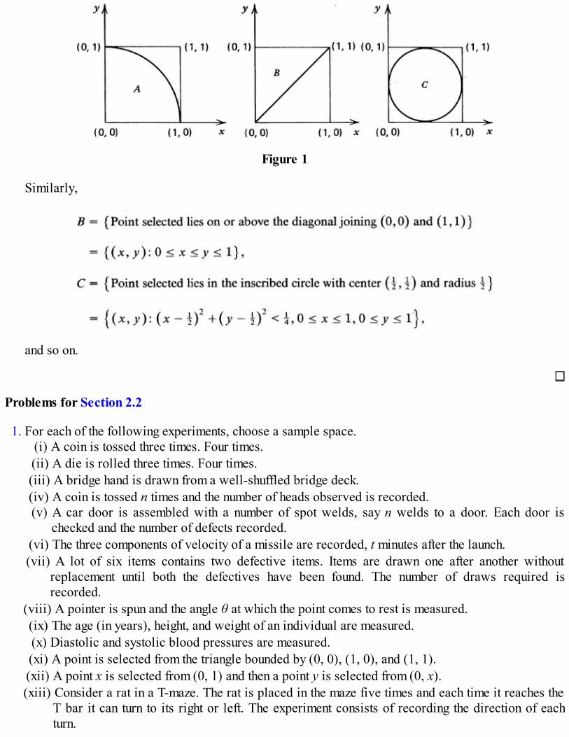
Figure 1

Similarly,

and so on.

Problems for Section 2.2

1. For each of the following experiments, choose a sample space.(i) A coin is tossed three times. Four times.(ii) A die is rolled three times. Four times.(iii) A bridge hand is drawn from a well-shuffled bridge deck.(iv) A coin is tossed n times and the number of heads observed is recorded.(v) A car door is assembled with a number of spot welds, say n welds to a door. Each door is

checked and the number of defects recorded.(vi) The three components of velocity of a missile are recorded, t minutes after the launch.(vii) A lot of six items contains two defective items. Items are drawn one after another without

replacement until both the defectives have been found. The number of draws required isrecorded.

(viii) A pointer is spun and the angle θ at which the point comes to rest is measured.(ix) The age (in years), height, and weight of an individual are measured.(x) Diastolic and systolic blood pressures are measured.(xi) A point is selected from the triangle bounded by (0, 0), (1, 0), and (1, 1).(xii) A point x is selected from (0, 1) and then a point y is selected from (0, x).(xiii) Consider a rat in a T-maze. The rat is placed in the maze five times and each time it reaches the

T bar it can turn to its right or left. The experiment consists of recording the direction of eachturn.

2. Consider a committee of three persons who vote on an issue for or against with no abstentionsallowed. Describe a suitable sample space and write as sets the following events.(i) A tie vote.(ii) Two “for” votes.(iii) More votes against than for.

3. Consider the population of all students at a state university. A student is selected. Let, A be the eventthat the student is a male, B the event that the student is a psychology major, C the event that thestudent is under 21 years of age.(i) Describe in symbols the following events:

(a) The student is a female, aged 21 years or over.(b) The student is a male under 21 years of age and is not a psychology major.(c) The student is either under 21 years of age or a male but not both.(d) The student is either under 21 or a psychology major and is a female.

(ii) Describe in words the following events:(a) A ∩ (B – C).(b) (A ∪ B ∪ C) – (A ∩ B) ∪ (B ∩ C) ∪ (A ∩ C).(c) A ∪ B ∪ C – A ∩ B.(d) B – (A ∪ C).(e) (A ∪ B ∪ C) – A ∩ B ∩ C.(f) A ∩ B – C.

4. Which of the following pairs of events are mutually exclusive?(i) Being a male or a smoker.(ii) Drawing a king or a black card from a bridge deck.(iii) Rolling an even-faced or odd-faced value with a die.(iv) Being a college student or being married.

5. Three brands of coffee, X, Y, and Z, are to be ranked according to taste by a judge. (No ties areallowed.) Define an appropriate sample space and describe the events “X preferred over Y,” “Xranked best,” “X ranked second best,” in terms of sets.

6. Three transistor batteries are put on test simultaneously. At the end of 50 hours each battery isexamined to see if it is operational or has failed. Write an appropriate sample space and identify thefollowing events:(i) Battery 2 has failed.(ii) Batteries 2 and 3 have either both failed or are both operational.(iii) At least one battery has failed.

7. A point is selected from the unit square bounded by (0, 0), (1, 0), (1, 1), and (0, 1). Identify thefollowing events:(i) The point lies on or above the diagonal joining (1, 0) and (0, 1).(ii) The point lies in the square bounded by ( , 0), (1, 0), (1, ), and ( , ).(iii) The point lies in the area bounded by y = 3x, y = 0, and x = 1.

8. Consider a 24-hour period. At some time x a switch is put into the ON position. Subsequently, at timey during the same 24 hour period, the switch is put into the OFF position. The times x and y are

recorded in hours, minutes, and seconds on the time axis with the beginning of the time period takenas the origin. Let Ω = {(x, y): 0 ≤ x ≤ y ≤ 24}. Identify the following events:

(i) The switch is on for no more than two hours.(ii) The switch is on at time t where t is some instant during the 24-hour period.(iii) The switch is on prior to time t1 and off after time t2 (t1 < t2 are two instants during the same 24-

hour period).

9. A sociologist is interested in a comparative study of crime in five major metropolitan areas. Sheselected Chicago, Detroit, Philadelphia, Los Angeles, and Houston for her study but decides to useonly three of the cities. Describe the following events as subsets of an appropriate sample space:

(i) Chicago is not selected.(ii) Chicago is selected but not Detroit.(iii) At least two of Chicago, Detroit, and Los Angeles are selected.(iv) Philadelphia, Detroit, and Los Angeles are selected.

10. There are five applicants for a job of which two are to be chosen. Suppose the applicants vary incompetence, 1 being the best, 2 the second best, and so on. The employer does not know these ranks.Write down an appropriate sample space for the selection of two applicants and identify thefollowing events:

(i) The best and one of the two poorest applicants are selected.(ii) The poorest and one of the two best are selected.(iii) At least one of the two poorest applicants is selected.

2.3 PROBABILITY AXIOMS

Consider a sample space Ω of a statistical experiment and suppose ζ is the class of events. We nowconsider what is usually the most difficult part of stochastic modeling, assigning probabilities to events inΩ. For completeness we need to be a little more specific about ζ.

DEFINITION 1*. A class ζ of subsets of Ω is said to be a sigma field (written “σ-field”) if it satisfiesthe following properties:

(i) Ω ∈ ζ,(ii) if A ∈ ζ, then ∈ ζ,

(iii) if A1, A2,… ∈ ζ, then An ∈ ζ,(iv) if A1, A2,… ∈ ζ, then An ∈ ζ.

We note that (iv) follows easily from (ii) and (iii). We are not greatly concerned in this course withmembership in class ζ. The reader needs to remember only that (a) with every Ω we associate a class ofevents ζ, (b) not every subset of Ω is an event, and (c) probability is assigned only to events (sets of classζ).

Consider a random experiment with sample space Ω and let ζ be the class of events. Let A ∈ ζ be anevent. How do we quantify the degree of uncertainty in A? Suppose the experiment is repeated† n timesand let f(A) be the frequency of A, that is, the number of times A happens. Due to statistical regularity, wefeel that the relative frequency of A, namely, f(A)/n, will stabilize near some number pA as n → ∞. That

is, we expect that

It is therefore tempting to take (1) as a definition of the probability of event A. There are both technicaland operational problems in doing so. How do we check in any physical situation that the limit in (1)exists? What should be the value of n before we assign to event A probability f(A)/n? The probability ofan event A should not depend on the experimenter or on a particular frequency f(A) that one observes in nrepetitions. Moreover, in many problems it may be impractical to repeat the experiment.

Let us write for convenience

and examine properties of r(A). We note that

(i) 0 ≤ r(A) ≤ 1,(ii) r(A) = 0 if and only if f(A) = 0, that is, if and only if A never occurs in n repetitions,

(iii) r(A) = 1 if and only if f(A) = n, that is, if and only if A occurs in each of the n repetitions,(iv) if A and B are mutually exclusive, r(A ∪ B) = r(A) + r(B).

All these properties appear desirable in any measure of uncertainty. It is intuitively attractive also todesire that r(A) converge to some pA as n → ∞.

Based on these considerations, it is reasonable to postulate that probability of an event satisfies thefollowing axioms.

DEFINITION 2. Let Ω be a set of outcomes and ζ be the associated collection of events. A setfunction P defined on ζ is called a probability if the following axioms are satisfied:

Axiom I. 0 ≤ P(A) ≤ 1 for all A ∈ ζ. Axiom II. P(Ω) = 1.Axiom III. If { An } is a sequence of mutually exclusive events (Ai ∩ Aj = Ø for i ≠ j), then

.

Axiom III is much stronger than property (iv) of relative frequency and is the most useful from acomputational point of view. In an experiment that terminates in a finite number of outcomes, it is hard tosee why Axiom III is required. If the experiment is repeated indefinitely and we consider the combinedexperiment, there are events that can only be described by a countable number of sets. Consider, forexample, repeated tossings of a fair coin until a head shows up. Let us write Ai for the event that a headshows up for the first time on the i th trial, i = 1, 2,…, and let us write A for the event that a head will beobserved eventually. Then

and one needs Axiom III to compute P(A) from P(Ai), i = 1, 2,….In Definition 2 we do not require P(Ø) = 0 since it follows as a consequence of Axioms I and III.We first consider some examples.

Example 1. Uniform Assignment. We consider a sample space Ω that has a finite number, say n, of elements. Let Ω = { ω1,…, ωn} and let ζ be the set of all subsets of Ω. Each one point set { ωj } is called an elementary event. Suppose we define P on ζ as follows:For each j,

Then for any A ∈ ζ, A = ∪j{ωij} is a finite union of elementary events. Accordingly, we define

Then P on ζ satisfies Axioms I to III and hence is a probability. In particular, take

so that

where n(A) = number of elements in A. This assignment of probability is called the uniform assignment and is basic to the study of allgames of chance such as coin tossing, die rolling, bridge and poker games, roulette and lotteries.

According to the uniform assignment, a problem of computing the probability of an event A reduces tothat of counting the number of elements in A. It is for this reason that we devote Section 2.5 to the study ofsome simple counting methods.

We now take some specific examples of the uniform model.

Example 2. Coin Tossing. A coin is tossed and the up face is noted. Then Ω = { H, T}. Let us define P by setting

Then P defines a probability on (Ω, ζ), where ζ = { Ø, {H}, {T}, {H, T}}. If the coin is fair, we take p = since n(Ω) = 2.If a fair coin is tossed three times, then Ω has 8 sample outcomes

and we take p1 = p2 = ··· = p8 = . Thus

and so on.

Example 3. Round-off Error. Suppose the balances of checking accounts at a certain branch of a bank are rounded off to the

nearest dollar. Then the actual round-off error equals the true value minus the recorded (rounded off) value. If an outcome ω is the actualround-off error in an account, then

Clearly, n(Ω) = 101. Let us consider the assignment:

Then P defines a probability. The probability that the round-off error in an account is at least 2 cents is given by

We now consider some examples of experiments where Ω is countably infinite. This is typically thecase when we do not know in advance how many repetitions are required before the experimentterminates. Let Ω = { ω1, ω2,… } be a countable set of points and let ζ be the class of all subsets of Ω.Consider the assignment:

Set

Then

and for any collection { An } of disjoint events,

It follows that P defines a probability on (Ω, ζ).It should be clear that there is no analog of the uniform assignment of probability when Ω is countably

infinite. Indeed, we cannot assign equal probability to a countably infinite number of points withoutviolating Axiom III.

Example 4. Tossing A Coin Until First Head. Consider repeated tossings with a possibly loaded coin with P{H} = p, 0 ≤ p ≤ 1.The experiment terminates the first time a head shows up. Here Ω = { H, TH, TTH, TTTH,… } is countably infinite. For reasons that willbecome clear subsequently, consider the assignment

Then

Moreover,

is a geometric series with sum 1/r for |r| < 1. See Section 6.5 for some properties of this series.) It follows that P defines a

probability on (Ω, ζ). Let A = {at least n throws are required}. Then:

In particular, if p = 1/n, then† P(A) limn→∞(1 – 1/n)n–1 = 1/e.

Example 5. Number of Arrivals at a Service Counter. The number of arrivals at a service counter in a time interval of length thours is recorded. Then Ω = {0, 1, 2,… } and ζ is the class of all subsets of Ω. A reasonable assignment of probability, as we shall see, isthe following:

where λ > 0 is a constant. As usual, we postulate that P(A) = ∑k∈Apk . Then 0 ≤ P(A) ≤ 1, and

It follows that P defines a probability on ζ. If A = {no more than 1 arrival in 15 minutes}, then t = and

Finally, we consider some examples where Ω is a continuous sample space.

Example 6. Selecting a Point from [a, b]. Suppose a point is selected from the interval [a, b]. Then Ω = [a, b]. The outcome ω ∈[a, b]. Since Ω contains uncountably many points, we cannot assign positive probability to every one point set { ω }, ω ∈ Ω withoutviolating Axiom III. The events of interest here are subintervals of Ω since we are interested in the probability that the chosen pointbelongs to an interval [c, d], say, where [c, d] ⊆ [a, b]. As mentioned in Section 2.2, subintervals of [a, b], as also their unions andintersections, are events. (Indeed ζ is taken to be the smallest σ-field containing subintervals of Ω. This is called the Borel σ-field.)

How do we assign probability to events in ζ? In this case probability is assigned by specifying a method of computation. For example,let f be a nonnegative integrable function defined on Ω such that dx = 1. For any subinterval I of Ω, define

and if A ∈ ζ is a disjoint union of subintervals Ik of Ω, define

Then P defines a probability on Ω.In particular, what is the analog of the uniform assignment of probability? For convenience, take a = 0, b = 1. If the points ω ∈ Ω are

to be equally likely (as in the case when Ω is finite), each one point set must be assigned the probability 0. Intuitively, the probability thatthe number selected will be in the interval [0, ] should be and so also should be the probability that the number selected is in the

interval . Therefore a reasonable translation of the uniform assignment in the continuous case is to assign to every interval aprobability proportional to its length. Thus we assign to [c, d] ∈ ζ

This assignment is considered in detail in Section 7.2.

Example 7. Length of Life of a Transistor. The life length of a transistor (in hours) is measured. Then Ω = [0, ∞), and we take ζ tobe the class of events containing all subintervals of Ω. Let us define

where λ > 0 is a fixed constant. If A = (a, b) ⊆ Ω, then

We leave the reader to show that P is a probability on (Ω, ζ).

Example 8. Two-Dimensional Uniform Model. Let us now construct a two-dimensional analog of the uniform model. Suppose Ω ={(x, y): a ≤ x ≤ b, c ≤ y ≤ d }. Clearly all subrectangles of Ω and their unions have to be taken as events. Indeed ζ is taken to contain allsubsets of Ω that have a well-defined area. These are sets over which one can integrate. To each A ∈ ζ we assign a probabilityproportional to its area. Thus

This is a reasonable analog of the uniform assignment of probability considered in Example 6. According to this assignment, all sets ofequal area irrespective of their shape or relative position are assigned the same probability, and in this sense all outcomes are equally likely

To summarize, a probability model consists of a triple (Ω, ζ, P) where Ω is some set of all outcomes,ζ is the set of events, and P is a probability defined on events. We call (Ω, ζ, P) a probability model or aprobability space or a probability system. To specify this model, one lists all possible outcomes andthen all events of interest. If Ω is discrete, it suffices to assign probability to each elementary event, thatis, each one-point set. If Ω is an interval or some subset of , we specify a method of computing

probabilities. This usually involves integration over intervals (in one dimension) or rectangles (in two ormore dimensions).

Remark 1. Definition 2 says nothing about the method of assigning probabilities to events. Sinceprobability of an event is not observable, it cannot be measured exactly. Thus any assignment we makewill be an idealization, at best an approximation. Examples 1, 6, and 8 give some specific methods ofassigning probabilities to events. (See also Remark 2.) In the final analysis the problem of assigning aspecific probability in a practical situation is a statistical problem. If the assignment is poor, it is clearthat our model will give a poor fit to the observations, and consequently our inferences are not going to bereliable.

Remark 2. In statistics the word “random” connotes the assignment of probability in a specific way.The word “random” corresponds to our desire to treat all outcomes as equally likely. In the case when Ωis finite this means (Example 1) that the assignment of probability is uniform in the sense that eachelementary outcome is assigned probability 1/n(Ω). Thus “a card is randomly selected from a bridgedeck” simply means that each card has probability of being selected. We elaborate on this idea stillfurther in Section 2.8.

If, on the other hand, Ω ⊆ then the phrase “a point is randomly selected” in Ω simply means thatthe assignment of probability to events in Ω is uniform. That is, the point selected may be any point of Ωand the probability that the selected point falls in some subset (event) A of Ω is proportional to themeasure (length, area, or volume) of A as in Examples 6 and 8.

Remark 3. (Interpretation). The probability of an event is a measure of how likely the event is tooccur. How, then, do we interpret a statement such as P(A) = ? The frequentist or objective view, thatwe will adhere to, is that even though P(A) is not observable it is empirically verifiable. According tothis view, P(A) = means that in a long series of (independent) repetitions of the experiment theproportion of times that A happens is about one-half. We thus apply to a single performance of theexperiment a measure of the chance of A based on what would happen in a long series of repetitions. Itshould be understood that P(A) = does not mean that the number of times A happens will be one-half thenumber of repetitions. (See Sections 5.4 and 6.3.1.)

There is yet another interpretation of the probability of an event. According to this so-calledsubjective interpretation, P(A) is a number between 0 and 1 that represents a person’s assessment of thechance that A will happen. Since different people confronted with the same information may have differentassessments of the chance of A, their (subjective) estimates of the probability of A will be different. Forexample, in horse racing, the odds against various horses participating in a certain race as reported bydifferent odds makers are different, even though all the odds makers have essentially the same informationabout the horses. An important difference between the frequentist and subjectivist approach is that thelatter can be applied to a wider class of problems. We emphasize that the laws of probability we develophere are valid no matter what interpretation one gives to the probability of an event. In a wide variety ofproblems, subjective probability has to be reassessed in the light of new evidence to which a frequencyinterpretation can be given. These problems are discussed in Section 2.6.

Remark 4. (Odds). In games of chance, probability is stated in terms of odds. For example, in horseracing a $2 bet on a horse to win with odds of 2 to 1 gives a total return of (approximately) $6 if the horsewins the race. We say that odds against an event A are a to b if the probability of A is b /(a + b). Thusodds of 2 to 1 (against a horse) means that the horse has a chance of 1 in 3 to win. This means, inparticular, that for every dollar we bet on the horse to win, we collect $3 if the horse comes in first in the

race (see Section 3.7).

Remark 5. For any event A we know that 0 ≤ P(A) ≤ 1. Suppose A ≠ Ø or Ω. If P(A) is near (or equalto) zero we say that A is possible but improbable. For example, if a point is selected at random from theinterval [0, 1], then the probability of every one-point set is zero. It does not mean, for example, that theevent {.93} is impossible but only that it is possible (since .93 is a possible value) but highly improbable(or has probability zero). In the relative frequency sense, it simply means that in a long series ofindependent selections of points from [0, 1], the relative frequency of the event {.93} will be near zero.

If P(A) > we say that A is more likely than not, and if P(A) = we say that A is as likely or probableas not (or that it has 50–50 chance). If P(A) is close to 1 we say A is highly probable (or very likely), andso on.

Problems for Section 2.3

1. Which of the following set functions define probabilities? State the reasons for your answer.(i) Ω = (0, ∞), P(A) = 0 if A is finite, and P(A) = 1 if A is an infinite set.(ii) Ω = [0, 1], P(A) = dx where f(x) = 2x, 0 < x < 1 and zero elsewhere.(iii) Ω = {1, 2, 3,… }, P(A) = ∑x∈A p(x) where p(x) = , x = 1, 2,… .(iv) Let Ω = {1, 2, 3,…, 2n, 2n + 1} where n is a positive integer. For each A ⊆ Ω define P as

follows:

and

(v) Let Ω = {2, 3, 4, 5, 6}. Define p(y) = y/20, y ∈ Ω and for A ⊆ Ω, P(A) = ∑y∈Ap(y).(vi) Let Ω = {2, 3, 4, 5, 6}. Define P(A) = ∑y∈Ap(y), A ⊆ Ω, where p(y) = (5 – y)/10, y ∈ Ω.(vii) Let Ω = (0, 1). For an event A ⊆ Ω define P(A) = ∫A6x(1 – x) dx.

2. A pocket contains 4 pennies, 3 nickels, 5 dimes, and 6 quarters. A coin is drawn at random. Find theprobability that the value of the coin (in cents) drawn is:

(i) One cent.(ii) 25 cents.(iii) Not more than 5 cents.(iv) At least 5 cents.(v) At most 10 cents.

3. A lot consists of 24 good articles, four with minor defects, and two with major defects. An article ischosen at random. Find the probability that

(i) It has no defects.(ii) It has no major defects.(iii) It is either good or has minor defects.

4. An integer is chosen at random from integers 1 through 50. Find the probability that:(i) It is divisible by 3.(ii) It is divisible by 4 and 6.(iii) It is not larger than 10 but larger than 2.(iv) It is larger than 6.

5. There are five applicants for a job. Unknown to the employer, the applicants are ranked from 1 (best)through 5 (worst). A random sample of two is selected by the employer. What is the probability thatthe employer selects:(i) The worst and one of the two best applicants.(ii) At least one of the two best applicants.(iii) The best applicant.

6. Assuming that in a four-child family, the 16 possible sex distributions of children bbbb, bbbg, bbgb,bgbb, gbbb,…, gggg are equally likely, find the probability that(i) Exactly one child is a girl.(ii) At least one child is a girl.(iii) At most one child is a girl.(iv) The family has more girls than boys.

7. In order to determine which of three persons will pay for coffee, each tosses a fair coin. The personwith a different up face than the other two pays. That is, the “odd man” who tosses a head when theother two toss tails, or vice versa, pays. Assuming that all the eight outcomes HHH, HHT, HTH,THH, TTH, HTT, THT, TTT are equally likely, what is the probability that the result of one toss willdiffer from the other two?

8. A person has six keys in her key chain of which only one fits the front door to her house. She tries thekeys one after another until the door opens. Let ωj be the outcome that the door opens on the j th try, j= 1, 2,…, 6. Suppose all the outcomes are equally likely. Find the probability that the door opens(i) On the sixth try.(ii) On either the first or the fourth or the sixth try.(iii) On none of the first four tries.

9. Two contestants play a game as follows. Each is asked to select a digit from 1 to 9. If the two digitsmatch they both win a prize. (The two contestants are physically separated so that one does not hearwhat the other has picked.) What is the probability that the two contestants win a prize?

10. Three people get into an elevator on the first floor. Each can get off at any floor from 2 to 5. Find theprobability that:(i) They all get off on the same floor.(ii) Exactly two of them get off on the same floor.(iii) They all get off on different floors.

11. Five candidates have declared for the position of mayor. Assume that the probability that a candidatewill be elected is proportional to the length of his or her service on the city council. Candidate A hassix years of service on the council; Candidate B has three years of service; C has four years; D, threeyears; and E, two years. What is the probability that a candidate with less than 4 years of service will

be elected? More than 3 years?

12. Roulette is played with a wheel with 38 equally spaced slots, numbered 00, 0, 1,…, 36. In addition tothe number, each slot is colored as follows: 0 and 00 slots are green; 1, 3, 5, 7, 9, 12, 14, 16, 18, 19,21, 23, 25, 27, 30, 32, 34, 36 are red, and the remaining slots are black. The wheel is spun and a ballis rolled around its edge. When the wheel and the ball slow down, the ball falls into a slot giving thewinning number and winning color. (Bets are accepted only on black or red colors and/or on anynumber or on certain combinations of numbers.) Find the probability of winning on:

(i) Red.(ii) An even number (excluding zero).(iii) 1, 4, 7, 10, 13, 16, 19, 22, 25, 28, 31, 34.(iv) 1 or red or 1, 2, 3, 4, 5, 6.(v) 1 and red and 1, 2, 3, 4, 5, 6.

13*. Consider a line segment ACB of length a + b where AC = a and CB = b, a < b. A point X is chosen atrandom from line segment AC and a point Y from line segment BC. Show that the probability that thesegments AX, XY, and YB form a triangle is a/(2b). (Hint: A necessary and sufficient condition for thethree segments to form a triangle is that the length of each segment must be less than the sum of lengthsof the other two.)

14*. The interval (0, 1) is divided into three intervals by choosing two points at random. Show that theprobability that the three-line segments form a triangle is .

15*. The base and the altitude of a right triangle are obtained by picking points randomly from [0, a] and[0, b] respectively. Show that the probability that the area of the triangle so formed will be less thanab/4 is ( )(1 + ln 2).

16*. A point X is chosen at random on a line segment AB.(i) Show that the probability that the ratio AX/BX is smaller than a(a > 0) is a/(1 + a).(ii) Show that the probability that the length of the shorter segment to that of the longer segment is <

is .

2.4 ELEMENTARY CONSEQUENCES OF AXIOMS

Consider a random experiment with set of outcomes Ω. In Section 2.3 we saw that it is not necessary toassign probability P to every event in Ω. If suffices to give a recipe or a method according to which theprobability of any event can be computed. In many problems we either have insufficient information orhave little interest in a complete specification of P. We may know the probability of some events ofinterest and may seek the probability of some related event or events. For example, if we know P(A),what can we say about P( )? If we know P(A) and P(B), what can we say about P(A ∪ B) or P(A ∩ B)?In this section we derive some properties of a probability set function P to answer some of thesequestions. These results follow as elementary consequences of the three axioms and do not depend on theparticular assignment P on ζ.

Suppose the proportion of female students at a certain college is .60. Then the proportion of malestudents at this college is .40. A similar result holds for the probability of an event and is proved inProposition 2 below. Similarly if the proportion of students taking Statistics 100 is .05, that of students

taking Mathematics 100 is .18, and that of students taking both Mathematics 100 and Statistics 100 is .03,then the proportion of students taking Mathematics 100 or Statistics 100 is (.05 + .18 – .03) = .20. Asimilar result holds for the set function P and is proved in Proposition 3.

We begin with a somewhat obvious result. Since the event Ø has no elements it should have zeroprobability.

PROPOSITION 1. For the empty set Ø, P(Ø) = 0.

Proof. Since Ø ∩ Ø = Ø and Ø ∪ Ø = Ø, it follows from Axiom III that

Hence P(Ø) = 0.

In view of Proposition 1 we call Ø the null or impossible event. It does not follow that if P(A) = 0 forsome A ∈ ζ, then A = Ø. Indeed, if Ω = [0, 1], for example, then we are forced to assign zero probabilityto each elementary event { ω }, ω ∈ Ω. Note also that if P(A) = 1, then it does not follow that A = Ω.

PROPOSITION 2. Let A ∈ ζ. Then:

Proof. Indeed, A ∩ = Ø and A ∪ = Ω, so that in view of Axioms II and III,

Proposition 2 is very useful in some problems where it may be easier to compute P( ).

Example 1. Rolling a Pair of Dice. Suppose a pair of fair dice is rolled. What is the probability that the sum of face values is at least5? Here

has 36 outcomes. Since the dice are fair, all pairs are equally likely and

By Proposition 2:

A direct computation involves counting the number of elements in the event

which, though not difficult, is time-consuming.

PROPOSITION 3. Let A, B ∈ ζ, A and B being not necessarily mutually exclusive. Then

Proof. A Venn diagram ( Figure 1) often helps in following the argument here. It suggests that theevents A ∩ , A ∩ B, and B ∩ are disjoint, so that by Axiom III,

Since, however,

Figure 1. Venn diagram for A ∪ B.

we have (again Axiom III):

Substituting for P(A ∩ ) and P(B ∩ ) from (4) and (5) into (3), we get (2).

COROLLARY 1. If A, B, C ∈ ζ, then:

Proof. Writing A ∪ B ∪ C = (A ∪ B) ∪ C and applying Proposition 3 twice, we get (6).

COROLLARY 2. For A1, A2,…, An ∈ ζ

Proof. The proof follows by mathematical induction.

COROLLARY 3. If A and B ∈ ζ, then

Proof. Since P(A ∩ B) ≥ 0, the result (8) follows from Proposition 3.

COROLLARY 4. If A1, A2,…, An ∈ ζ, then

Proof. Follows from (8) by induction on n.

It should be clear by now that Axiom III is the only way to compute probabilities of compound events.The property of Axiom III is called additivity and that of Corollaries 3 and 4 is called subadditivity. Theextension of (9) to countable number of events is given below.

In statistics, probability bounds such as (9) are often useful. For example, let P(A) = .4 and P(B) = .2and suppose we want P(A ∪ B). If A and B are not mutually exclusive, we cannot compute P(A ∪ B)exactly unless we know P(A ∩ B). See relation (2). Corollary 3, however, tells us that P(A ∪ B) ≤ .6. Infact, even though we do not know P(A ∪ B) exactly, we can conclude that .4 ≤ P(A ∪ B) ≤ .6. Theinequality on the left follows from Proposition 4 (Corollary 2) below.

Example 2. Lottery. Consider a promotional lottery run by a mail-order magazine clearing house. Suppose 1 million entries arereceived. There are 10 prizes, and prizes are awarded by a random drawing. This means uniform assignment of probability so that eachticket has 10/106 chance of winning a prize. Suppose someone sends in three entries, what is the probability of this person winning at leastone prize? Let Ak be the event that the k th ticket wins a prize. Then the event that the person wins at least one prize is

where A1, A2, A3 are not mutually exclusive. We cannot apply Axiom III, but (6) is applicable and certainly Corollary 4 is applicable. Inview of Corollary 4,

Thus even though we have not evaluated the exact probability, we are able to say that it is highly improbable that he or she will win a

prize.

Example 3. Random Selection from Freshman Class. The freshman class at a college has 353 students of which 201 are women,57 are majoring in mathematics, and 37 mathematics majors are women. If a student is selected at random from the freshman class, whatis the probability that the student will be either a mathematics major or a woman?

Each of the 353 students has probability 1/353 of being selected. Let M be the event that the student is a mathematics major and W bethe event that the student is a woman. Then

and from (2),

Let A, B ∈ ζ such that A ⊆ B. Is A more probable than B? The answer is no.

PROPOSITION 4. Let A, B ∈ ζ such that A ⊆ B. Then

Proof. Indeed, since A ⊆ B, A ∩ B = A so that from (5)

COROLLARY 1. For An ∈ ζ, n = 1, 2,…

Proof. We have

COROLLARY 2. max{ P(A), P(B)} ≤ P(A ∪ B) ≤ min{ P(A) + P(B), 1).

PROPOSITION 5. Let A, B ∈ ζ, then

and, more generally,

Proof. We have

so that

In the general case:

so that

COROLLARY 1. min{ P(A), P(B)} ≥ P(A ∩ B) ≥ max{0, 1 – P( ) – P( )}.

Example 4. Highly Probable Events. Suppose that in a metropolitan area 80 percent of the crimes occur at night and 90 percent ofthe crimes occur within the city limits. What can we say about the percentage of crimes that occurs within the city limits at night?

Let A be the event “crime at night” and B be the event “crime within city limits.” Then P(A) = .80 and P(B) = .90, so that fromProposition 2, P( ) = .20 and P( ) = .10. In view of (12),

so that the probability of both a crime occurring at night and a crime occurring within the city limits is at least .70. Note that P(A ∩ B) ≤.8.

It should be noted that the bounds (8) and (12) may yield trivial results. In Example 4, if we want P(A ∪ B), then the bound (8) yieldsP(A ∪ B) ≤ .8 + .9 = 1.7 which, though correct, is useless. Similarly, if P(A) = .3 and P(B) = .1, then (12) yields

which, though true, is of no use.

Problems for Section 2.4

1. A house is to be given away at a lottery. Tickets numbered 001 to 500 are sold for $200 each. Anumber is then randomly selected from 001 to 500 and the person with the corresponding ticket winsthe house. Find the probability that the number drawn will be:

(i) Divisible by 5.(ii) Not divisible by 5.(iii) Larger than 200 and not divisible by 5.(iv) Divisible by 5 but not 10.(v) Divisible by 5, 6, and 10.

2. The probability that a customer at a bank will cash a check is .72, the probability that he will ask tohave access to his safety deposit box is .09, and the probability that he will do both is .003. What isthe probability that a customer at this bank will either cash a check or ask to have access to his safetydeposit box? What is the probability that he will do neither?

3. Let P(A) = .12, P(B) = 0.89, P(A ∩ B) = .07. Find:(i) P(A ∪ B).(ii) P(A ∪ ).(iii) P(A ∩ ).(iv) P( ∪ B).(v) P( ∪ ).(vi) P( ∩ B).

4. Suppose A, B, and C are events in some sample space Ω and the following assignment is made:

Find the following probabilities whenever possible. If not, find lower and upper bounds for theprobability in question.

(i) P( ).(ii) P(A ∪ ).(iii) P(B ∩ C).(iv) P( ∪ ).(v) P( ∩ ).(vi) P(A ∪ B ∪ ).(vii) P(A ∩ C) + P( ∩ C).

5. Consider a large lot of spark plugs. The company looks for three kinds of defects, say A, B, and C, inthe plugs it manufactures. It is known that .1 percent of plugs have defects of type A, 1 percent ofplugs have defects of type B, and .05 percent of plugs have defects of type C. Moreover, .05 percentof plugs have defects of type A and B, .02 percent have defects of type B and C, .03 percent havedefects of type A and C, and .01 percent have all three defects. What is the probability that a sampledplug from the lot is defective, that is, has at least one of the three defects?

6. Let A and B be two events. Then A Δ B is the (disjoint) union of events A – B and B – A. That is, A Δ Bis the event that either A happens or B but not both. Show that:

7. A number is selected at random from the unit interval [0, 1]. What is the probability that the numberpicked will be a rational number? (Hint: The set of rational numbers is countable.)

8. Let Ω = (0, ∞) and for each event A define P(A) = ∫Ae–ω dω. What is the probability of the event:

9. Tom was interviewed by three prospective employers. On the basis of his interviews he estimates thathis chances of being offered a job by the three employers are, respectively, .8, .9, .75. What can yousay about his chances of being offered all three jobs?

10. A manufacturer of magnetic tapes for tape decks checks the tapes for two types of defects: improperlyapplied magnetic coating, and tear or wrinkles in the tape. It is known that about .06 percent of thetapes have coating defects, about .02 percent have wrinkles or tears, and about .015 percent haveboth defects. Find the probability that a customer will receive:

(i) a defective tape,(ii) a nondefective tape.

11. It is estimated that a certain bill has an 80 percent chance of being passed by the House ofRepresentatives, a 90 percent chance of being passed by the Senate and a 95 percent chance of beingpassed by at least one chamber.

(i) What is the probability that the bill will come before the President for signatures?(ii) What is the probability that it will pass one of the chambers but not the other?(iii) What is the probability that it will be passed by neither chamber?

12. The probability that Trent will buy a car this year is .90, that he will buy a video cassette recorder is.80, that he will buy a home computer is .95, and that he will buy a car as well as a video cassetterecorder is .75. What is your best estimate of the lower bound of the probability that he will buy allthree?

13. In a sample survey of 100 students at a university, the students were asked the following question:Which of the three magazines A, B, or C do you read? The following results were obtained:55 read A 28 read A and B 22 read all three42 read B 32 read B and C 69 read C 44 read A and C If a student is selected at random from these 100 students, find the probability that she reads:

(i) Only A.(ii) Only B.(iii) Only C.(iv) Only A or B.

(v) None of the three.(vi) At least one.(vii) At most one.(viii) Exactly two.(ix) At least two.

14. A study of a busy metropolitan airport yielded the following estimates of probabilities for the numberof airplanes waiting to land at a peak hour:

Find the probability that(i) At least two planes are waiting to land.(ii) No more than three planes are waiting to land.(iii) At most five planes are waiting to land.(iv) More than two planes are waiting to land.

15. In a study of herpes victims it is found that 50 percent are women, 95 percent are white, 80 percentare 20–40 years of age, 55 percent have had at least four years of college, and 55 percent earn over$20,000 a year. Find bounds on the probability that a randomly chosen victim

(i) Is white and aged 20–40 years.(ii) Has had four years of college and earns more than $20,000 a year.(iii) Is nonwhite or not aged 20–40 years.

2.5 COUNTING METHODS

Let Ω be a finite sample space with n elements. According to the uniform assignment of probability, if A⊆ Ω, then

where n(A) = the number of elements in A. This assignment reduces the problem of probabilitycomputation to that of counting. In this section we consider some rules that facilitate counting. Oursubsequent development is not crucially dependent on the knowledge of these rules. Their knowledgedoes, however, help simplify computations.

We begin with the simplest and yet the most important rule, from which all the remaining rules will bederived.

Rule 1. Let A = { a1, a2,…, am } and B = {b1, b2,…, bn} be two sets. Then the number of pairs (aj, bk)where aj ∈ A and bk ∈ B that can be formed is mn. That is, the product set A × B has mn elements.Proof. Let us arrange the pairs in a rectangular array (or an m × n table), as follows.

The assertion of Rule 1 is now obvious. An alternative but frequently used method is to draw a treediagram, such as in Figure 1. We first draw an element from A and then an element from B. The result ofthe first draw is exhibited by m branches emanating from a point. Each branch corresponds to one andonly one element of A. The result of the second draw is represented by n branches emanating from a1, a2,…,am. The total number of pairs is simply the total number of branches after the second draw, namely,mn.

Figure 1. Tree diagram.

COROLLARY 1. Let Aj = { aj,1, aj,2,…, aj, nj}, j = 1, 2,…, k. Then the total number of ordered k-

tuples (a1, i1, a2, i2,…, ak , ik) that can be formed by taking one element from each set (in the order A1, A2,…, Ak) is given by n1n2 ··· nk. That is, the number of elements in the product set A1 × A2 × ··· Ak is n1n2··· nk.

Proof. For k = 2, this is simply Rule 1. Now proceed by induction. A tree diagram makes the resulttransparent.

COROLLARY 2. (Sampling with Replacement-Ordered Samples ). The number of ordered k-tuples(ai1,…, aik) where aij ∈ A = {a1, a2,…, an) is nk. (The term with replacement refers to the fact that thesymbol drawn on any draw is replaced before the next draw is made.)

Proof. In Corollary 1, take A1 = A2 = ··· = Ak = A.

Example 1. Number of License Plates. Suppose a license plate in a state consists of three letters of alphabet followed by twointegers from 0 to 9. What is the total number of license plates possible?

We take A1 = A2 = A3 = {A, B,…, Z}, A4 = A5 = {0, 1, 2,…, 9} in Corollary 1 to Rule 1. Then n1 = n2 = n3 = 26, n4 = n5 = 10 and

the number of possible license plates is (26)3(10)2 = 1,757,600.

Example 2. Sex Distribution of Children. Consider families with five children. Let us write b for a boy and g for a girl and write thesexes of children in order of their ages. How many different distributions are possible? Let us take A = {b, g} , n = 2 and k = 5 inCorollary 2 to Rule 1. The number of possible sex distributions is 2 · 2 · 2 · 2 · 2 = 25 = 32.

Similarly, if we consider families with n children, then there are 2n different sex distributions.

Often sampling is done without replacement, that is, an item drawn is not replaced before the nextdraw. There are two cases to consider: (i) when order matters, (ii) when order does not matter.

Rule 2. (Ordered Samples Without Replacement) . The number of ordered k-tuples (ai1, ai2,…, aik),where aij ∈ A = { a1, a2,…, an) and repetition is not allowed (that is, no two aij’s are the same), is givenby

Proof. Since repetition is not permitted at each draw, one loses exactly one element. Applying Corollary1 to Rule 1 with n1 = n, n2 = n – 1,…, nk = n – k + 1, the assertion follows.

COROLLARY 1. The number of ordered n-tuples (ai1, ai2,…, ain) where aij ∈ A = { a1, a2,…, an}

and repetition is not allowed is n(n – 1) ··· 2 · 1.

Proof. Take k = n in Rule 2.

The number nPk is sometimes called the number of permutations of k objects out of n or the number ofpermutations of n objects taken k at a time. In the special case when k = n (Corollary 1) nPn represents areordering or permutation of n objects. For convenience we write

It follows that

for integers 0 ≤ k ≤ n, and we set nPk = 0 for integers k > n. We adopt the convention that 0! = 1.

Example 3. Management Committee. From the five-member board of directors of a company, a three-member managementcommittee is to be selected, consisting of a chairman, a treasurer, and a secretary. Since order matters, and sampling is withoutreplacement (it matters whether a member is secretary or treasurer and a member cannot be both), we use Rule 2 with n = 5 and k = 3.The number of possible committees is 5P3 = 5 · 4 · 3 = 60.

Example 4. Photographer’s Dilemma. The photographer of a small-town newspaper is asked to take pictures at a swim meet.Some of the pictures are to be included along with the results of the meet in a forthcoming edition of the paper. The photographer takes 20pictures, all of which turn out well. The editor tells the photographer to select two and to decide on the order in which they will appear inthe paper. How many possible choices are there? Using Rule 2 with n = 20 and k = 2, we see that the photographer has 20(19) = 380possible choices.

Let us now consider a case when the order in which the objects are drawn does not matter. In thiscontext we speak of population and subpopulation. A population (subpopulation) of size n is a collectionof n objects without regard to order. We say that two populations (or subpopulations) are different if andonly if they have at least one element that is not common to both.

Rule 3. (Unordered Samples Without Replacement) . The number of subpopulations of size k or thenumber of unordered subsets {ai1,…, aik } or the number of ways of selecting k distinct objects out of nobjects in A = { a1, a2,…, an } is

Proof. Let x be the number of subpopulations of size k drawn from n objects {a1, a2,…, an }. We note thatthere are nPk ordered k-tuples (ai1, ai2,…, aik) where aij ∈ A. Each of the k! possible permutations of (ai1,ai2,…, aik) leads to the same subpopulation {ai1, ai2,…, aik}. Hence

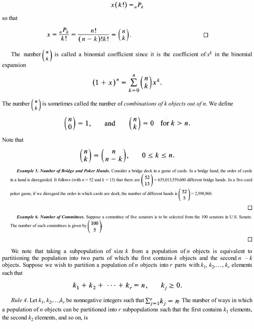
so that

The number is called a binomial coefficient since it is the coefficient of xk in the binomial

expansion

The number is sometimes called the number of combinations of k objects out of n. We define

Note that

Example 5. Number of Bridge and Poker Hands. Consider a bridge deck in a game of cards. In a bridge hand, the order of cards

in a hand is disregarded. It follows (with n = 52 and k = 13) that there are = 635,013,559,600 different bridge hands. In a five-card

poker game, if we disregard the order in which cards are dealt, the number of different hands is = 2,598,960.

Example 6. Number of Committees. Suppose a committee of five senators is to be selected from the 100 senators in U.S. Senate.

The number of such committees is given by .

We note that taking a subpopulation of size k from a population of n objects is equivalent topartitioning the population into two parts of which the first contains k objects and the second n – kobjects. Suppose we wish to partition a population of n objects into r parts with k1, k2,…, kr elementssuch that

Rule 4. Let k1, k2,…,kr be nonnegative integers such that . The number of ways in whicha population of n objects can be partitioned into r subpopulations such that the first contains k1 elements,the second k2 elements, and so on, is

Proof. We first select k1 elements from n in ways; of the remaining n – k1 elements we select k2

elements in ways, and so on. By Corollary 1 to Rule 1, the number of such partitions is

since n – k1 – ··· – kr–1 = kr. (We note that we can make only r – 1 choices, the last one being determinedautomatically.)

The numbers are called multinomial coefficients since they appear as coefficients in the

multinomial expansion

Example 7. Grade Distribution. A class of Ω students is to be divided in such a way that two students get A’s, 2 get B’s, 5 get C’sand 3 get D’s. Then the number of possible grade distributions is given by

The following diagram summarizes the results of this section.

Applications to Probability

We recall that when Ω is finite and the probability assignment is uniform

We now consider some applications.We can use the metaphor of balls and cells to describe the sampling process in a wide variety of

applications. Thus k balls can be randomly distributed in n cells in nk different ways. This follows fromRule 1, since we need to choose one cell for each of the k balls. Thus the experiment of throwing a die ktimes has 6k possible outcomes. If we require that no cell has more than one ball, that is, there is norepetition, then Rule 2 gives the number of distributions to be nPk, k ≤ n. If all possible distributions havethe same probability n–k, then the probability that no cell has more than one ball is given by nPk/nk.

Example 8. Elevators, Subway Trains, and Birthdays.

(i) An elevator starts with k = 5 passengers and stops at n = 6 floors. The probability that no two passengers alight at the same flooris 6P5/65 = 5/54.

(ii) A subway train has n cars and is boarded by k passengers (k ≤ n). Suppose the passengers choose cars randomly. Then theprobability that all passengers will board different cars is nPk /nk . In particular, if k = n = 6, then this probability is 5/324 =.015432, a rather improbable event.

(iii) Consider a class of k students. The birthdays of these students form a sample of size k from the population of n = 365 days in theyear (assuming that all years are of equal length). Then the probability that all k birthdays will be different is 365Pk /(365)k , and

the probability that at least two students will have the same birthday is {1 – 365Pk /(365)k}. The following table gives pk =

365Pk /(365)k for some selected values of k .

We note that in a class of 23 students the probability is 1 – .493 = .507 that at least two students will have a common birthday,whereas in a class of 35 students this probability is .814.

Example 9. Four Bridge Players Holding an Ace Each. A bridge deck of 52 cards can be partitioned into four hands of 13 cardseach in 52!/(13!)4 ways. What is the probability that every player has an ace? We note that the four aces can be permuted (Rule 2) in 4!

ways. Each permutation represents exactly one way of giving one ace to each player. The remaining 48 cards can be partitioned (by Rule4) into four groups of Ω cards each in 48!/(12!)4 ways. By Rule 1, the number of distributions where each player holds an ace is (4!)[48!/(12!)4], so that the required probability is

Example 10. Selecting Line Segments Randomly to Form a Triangle. Given five line segments of lengths 1, 3, 5, 7, 9 centimeters,What is the probability that three randomly selected line segments will form a triangle? Clearly the order of selection is not important. It

follows from Rule 3 that there are = 10 possible ways of selecting three line segments out of five, each of which has the same

probability of being selected, namely 1/10. Next we note that in order for any three line segments to form a triangle, the sum of any twoline segments must be greater than the third. Since only three selections {3, 5, 7; 5, 7, 9; 3, 7, 9} meet this requirement, the probability is3/10.

Example 11. Absent-minded Professor. Consider a professor who signs five letters of references for one of his students and thenputs them into five preaddressed envelopes at random. What is the probability that none of the letters is put in its correct envelope? ByRule 2 the number of elements in Ω is 5! = 120 so that each outcome is assigned the probability of 1/120. Let Ai be the event that the i thletter is placed in the correct envelope. Then the probability we seek is 1 – . From Corollary 2 to Proposition 2.4.3, wehave:

To compute P(Ai), we note that since the i th letter goes to its correct envelope, the number of random distributions of the remaining fourletters is 4!. Hence P(Ai) = 4!/5! = 1/5 = .20.

Exactly the same argument applies to P(Ai ∩ Aj), P(Ai ∩ Aj ∩ Ak), and so on. We have:

It follows that

so that the required probability is 11/30.If there are n envelopes and n letters, then the probability that at least one letter is put into its correct envelope is given by

It follows that the probability that none of the letters is put into its correct envelope → e–1 = .3679 as n → ∞.

Example 12. Parking Tickets. In some cities, overnight street parking is not allowed. A person who got 10 tickets for overnightstreet parking noticed that all the tickets were issued on Mondays, Tuesdays, and Fridays. Would she be justified in renting a garage only

for those nights? (That is, do the police have a system?) Let us assume randomness, that is, that the police have no system and randomlypatrol the city. Then the total number of distributions of 7 days (n = 7) to 10 tickets (k = 10) is 7 (each ticket is assigned one of the sevendays). Of these, there are 310 ways of assigning the three days to each ticket. Hence, under the assumption that the police do not have asystem, the probability of being ticketed 10 times on Mondays, Tuesdays, and Fridays is (3/7)10 = .0002. In other words, if the streetswere patrolled randomly then it is highly improbable that in a selection of 10 tickets all will be issued on Mondays, Tuesdays, and Fridays.This small probability casts doubt on our assumption that the streets are patrolled randomly.

Suppose that in 10 tickets none is given on Saturdays. Is there sufficient evidence to conclude that no tickets are issued on Saturdays?Proceeding exactly as above, the probability that all 10 tickets are issued on Sundays through Fridays, assuming randomness, is (6/7)10 =.2141. Since this probability is not small, the evidence does not justify the conclusion that no tickets are issued on Saturdays.

Problems for Section 2.5

1. A restaurant menu lists three soups, eight meat dishes for the main course, ten desserts, and sevenbeverages. In how many ways can a full meal be ordered consisting of one soup, one meat dish, onedessert, and one beverage?

2. A nationwide fast-food chain used to advertise that it could serve hamburgers in 256 ways. What isthe number of choices of “fixings” (lettuce, ketchup, onion, pickles, etc.) that the chain offers?

3. A Social Security number consists of nine digits. How many different Social Security numbers canthere be?

4. Find the number of different four-digit numbers larger than 2000 that can be formed with digits 1, 2, 3,4 if(i) No repetitions are allowed.(ii) Repetitions are allowed.

5. Find the number of different four-letter words that can be formed from letters in the word LOVE when(i) No repetitions are allowed.(ii) Repetitions are allowed.

6. In baseball’s World Series, the first team that wins four games out of seven possible games wins theSeries. Find the number of ways in which the Series can end.

7. In how many different ways can you permute letters of the word INSTRUMENTS?

8. Find the number of different seven-digit telephone numbers that can be formed if(i) The first digit must be 3 and second 2.(ii) The first digit must be 3 and no repetitions are allowed.

9. Each permutation of the digits 1, 2, 3, 4, and 5 determines a five-digit number. If numberscorresponding to all possible permutations are listed in increasing order of magnitude beginning with12345, what is the 96th number in this list?

10. In how many different ways can seven people be seated around a circular table?

11. A professor tells exactly three jokes a semester in his course. If it is his policy never to repeat thesame combination of three jokes,

(i) How many semesters will eight jokes last him?(ii) What is the minimum number of different jokes he will tell in 35 semesters? 20?

12. A young woman has four suitors. A gypsy tells the woman that she will be married twice and that bothher husbands will come from this group of four men. How many marital histories are possible for thiswoman?

13. Ten friends meet at a party and shake hands. How many handshakes are exchanged if each personshakes hands with every other person once and only once?

14. Find out how many ways a student can answer a 20-problem true/false examination if(i) She marks half the questions true and the other half false.(ii) She marks no two consecutive answers the same.

15. What is the possible number of bridge hands that can consist of seven spades, three hearts, twodiamonds, and one club?

16. A die is tossed ten times. Find the number of ways in which 1 appears two times, 2 appears threetimes, 3 appears one time, 4 appears two times, and 5 appears two times.

17. In a survey of students at a state university, 20 students were asked to respond to the followingquestion: “Are you in favor of holding classes on Saturdays? Answer yes, no, no opinion.” What isthe number of ways in which 5 of the respondents can answer yes, Ω answer no, and 3 answer noopinion?

18*. Find the number of unordered sets (subpopulations) {ai1, ai2,…, aik } where aij ∈ A = {a1, a2,…, an}when repetition is allowed. (The answer gives the rule for unordered sampling with replacement andcompletes the diagram on page 38.)

19. The automobile license plates issued in a certain state have three digits followed by three letters. Alicense plate number is selected at random, and the person whose license plate matches the numberwins a new car. If you have three cars registered in this state, what is your chance of winning the newcar?

20. From six positive and 10 negative numbers, four are picked at random (without replacement) andmultiplied. What is the probability that the product is negative?

21. A five-person Credentials Committee is to be chosen from a group of nine men and six womendelegates to a national convention. If all the members of the committee selected are men, do womenhave reason to complain?

22. A lot of 100 fuses is known to contain 20 defective fuses. If a sample of 15 fuses contains only onedefective fuse, is there reason to doubt the randomness of the selection?

23. In a game recently run by a well-known fast-food restaurant chain, each customer is given a card withΩ squares. The customer is allowed to scratch exactly three squares to reveal whether a square ismarked yes or sorry. Three yeses win a prize. Suppose five squares are marked yes and sevenmarked sorry. What is the probability that a customer will win a prize?

24. A closet contains six pairs of shoes. Four shoes are selected at random. What is the probability thatamong the four shoes there will be:

(i) Exactly one pair,(ii) At least one pair.

25. (i) A married couple and four of their friends enter a row of seats in a concert hall. What is theprobability that the wife will sit next to her husband if all possible seating arrangements areequally likely?

(ii) In part (i), suppose the six people go to a restaurant after the concert and sit at a round table. Whatis the probability that the wife will sit next to her husband?

26. In a five-card poker game, find the probability that a hand will have:(i) A royal flush (ace, king, queen, jack, and ten of the same suit).(ii) A straight flush (five cards in a sequence, all of the same suit; ace is high but A, 2, 3, 4, 5 is also

a sequence) excluding a royal flush.(iii) Four of a kind (four cards of the same face value).(iv) A full house (three cards of the same face value x and two cards of the same face value y).(v) A flush (five cards of the same suit excluding cards in a sequence).(vi) A straight (five cards in a sequence).(vii) Three of a kind (three cards of the same face value and two cards of different face values).(viii) Two pairs.(ix) A single pair.

27*. Consider a town with N people. A person sends two letters to two separate people, each of whom isasked to repeat the procedure. Thus for each letter received, two letters are sent out to separatepersons chosen at random (irrespective of what happened in the past). What is the probability that inthe first n stages the person who started the chain letter game will not receive a letter?

28. Consider a town with N people. A person tells a rumor to a second person, who in turn repeats it to athird person, and so on. Suppose that at each stage the recipient of the rumor is chosen at random fromthe remaining N – 1 people. What is the probability that the rumor will be repeated n times

(i) Without being repeated to any person.(ii) Without being repeated to the originator.

29. A lot of 15 items contains two defective items. Two items are drawn at random (withoutreplacement). Find the probability that

(i) Neither is defective.(ii) At least one is not defective.

30. In order to raise money for its Pee Wee League baseball team, a club runs a lottery at its annualpicnic. There is exactly one grand prize. Each participant draws a ticket from a box; the winningnumber is to be announced after all participants have drawn their tickets. Two customers, Jones andPaul, arrive at the same time and Jones is allowed to draw a ticket first. Paul complains that this isunfair since if Jones has drawn the grand prize, Paul has no chance. Is Paul justified in complaining?

31. A local bank has a time-and-temperature service that is repeated over the telephone every 15 seconds.The members of a local swimming team are advised to call the service before coming for morning

practice. If the temperature is below 60°F there is no practice. On a certain day 30 people showed upfor practice. All claimed that they called the time and temperature number during the 30-minuteperiod 6:00 a.m. to 6:30 a.m. and none of the callers received a busy signal. Do you have any reasonto doubt their claim? (Assume that if two or more calls are received in any 15-second period duringwhich the report is being given, the callers receive a busy signal.)

32. There were four accidents in a town during a seven-day period. Would you be surprised if all fouroccurred on the same day? Each of the four occurred on a different day?

33. Consider the lottery of Example 2.4.2, where 1 million entries are received and 10 prizes are to beawarded by a random drawing. What is the probability that a person who sends in three entries willwin at least one prize?

2.6 CONDITIONAL PROBABILITY

Let (Ω, ζ, P) be a probability model for some random experiment. We recall that P is defined on events,that is, on elements of ζ, and for A ∈ ζ, P(A) may be thought of as a measure of our belief in theuncertainty of A prior to a performance of the experiment. Often, however, some information becomesavailable while the experiment is in progress. For example, suppose we know that about 50 percent ofpeople over age 40 are overweight and suppose that the percentage of people who are overweight andhave heart disease is 25. A person is randomly chosen from an over-40 age group and is found to beoverweight. How do we use this information to compute the probability that the person has heart disease?How do we modify our model to take this information into account?

Formally, suppose A ∈ ζ and we are told that A has happened. What is the probability that B has alsohappened? That is, suppose the outcome is a point in A. What is the probability that it is also in B or, toput it alternatively, what is the probability that event A was “caused” by B? Since the outcome ω ∈ A, weknow that ω ∉ , so that all subsets of should get zero probability. Moreover, ω ∈ A and ω ∈ B ifand only if ω ∈ A ∩ B, so that we should assign to B the proportional mass P(A ∩ B)/P(A). This is theproportion of event A “occupied” by B (see Figure 1). We are led to the following definition.

DEFINITION 1. (CONDITIONAL PROBABILITY). Let A ∈ ζ be such that P(A) > 0. Then theconditional probability of B ∈ ζ given A, written P{ B|A}, is defined by

Figure 1. Part of A occupied by B, A ∩ B.

In the example above, the (conditional) probability that a randomly selected person over 40 years ofage will have heart disease, given that he or she is overweight, is .

Are we justified in calling P( B|A} a probability? Does P{ ·|A } satisfy the three probability axioms?Clearly 0 ≤ P(B|A) ≤ 1 for all B ∈ ζ since 0 ≤ P(A ∩ B) ≤ P(A). Moreover, P{A|A) = 1. Finally, if { An }is any sequence of mutually exclusive events, then

since { An ∩ A } are also mutually exclusive. We have thus shown that for each fixed A ∈ ζ with P(A) > 0,P{ ·|A } defines a probability on (A, ζ). It follows that it has all the properties of a probability describedin Section 2.3.

Remark 1. One can also motivate the definition of conditional probability in terms of relativefrequency. If the experiment is repeated n (independent) times, we look at all those cases where theoutcome is in A. If the outcome is also in B for a proportion pB|A times, then we should assign to B theprobability pB|A. The proportion of times A occurs is approximately P(A) while the proportion of thesewhen B also occurs is about P(A ∩ B), so that

Example 1. Distribution of Students by Sex and Declared Major. The distribution of 1237 students at a community college by sexand declared major is given below

If a business major is randomly selected from this college, what is the probability that the student is a female? Using uniform assignmentof probability, each student has the same chance, 1/1237, of being selected. Hence

Similarly,

Example 2. Lifetime of a Light Bulb. The lifetime of a light bulb is recorded in hours of use. Take Ω = [0, ∞). Let P be defined on

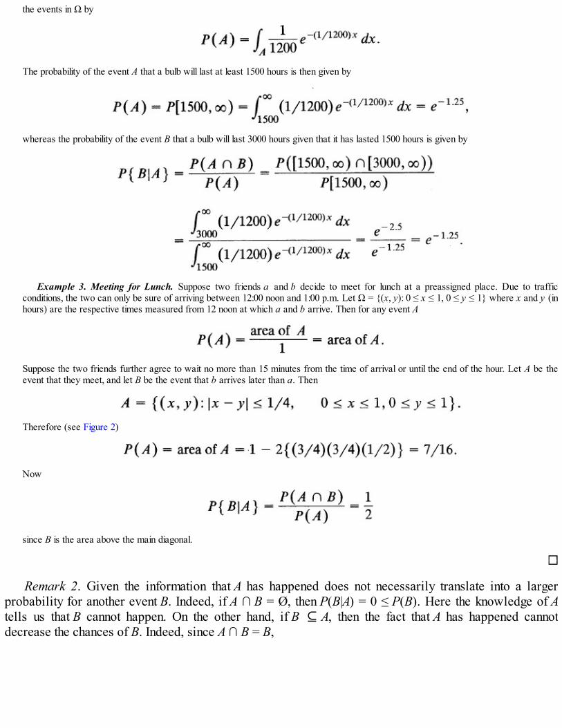
the events in Ω by

The probability of the event A that a bulb will last at least 1500 hours is then given by

whereas the probability of the event B that a bulb will last 3000 hours given that it has lasted 1500 hours is given by

Example 3. Meeting for Lunch. Suppose two friends a and b decide to meet for lunch at a preassigned place. Due to trafficconditions, the two can only be sure of arriving between 12:00 noon and 1:00 p.m. Let Ω = {(x, y): 0 ≤ x ≤ 1, 0 ≤ y ≤ 1} where x and y (inhours) are the respective times measured from 12 noon at which a and b arrive. Then for any event A

Suppose the two friends further agree to wait no more than 15 minutes from the time of arrival or until the end of the hour. Let A be theevent that they meet, and let B be the event that b arrives later than a. Then

Therefore (see Figure 2)

Now

since B is the area above the main diagonal.

Remark 2. Given the information that A has happened does not necessarily translate into a largerprobability for another event B. Indeed, if A ∩ B = Ø, then P(B|A) = 0 ≤ P(B). Here the knowledge of Atells us that B cannot happen. On the other hand, if B ⊆ A, then the fact that A has happened cannotdecrease the chances of B. Indeed, since A ∩ B = B,

Figure 2

If B ⊇ A, then trivially P{B|A} = 1.

Remark 3. The conditional probability P{B|A} remains undefined for P(A) = 0.

As a simple consequence of Definition 1, we note that

and,

Relations (1) and (2) are special cases of the so-called multiplication rule of probability.

PROPOSITION 1. (MULTIPLICATION RULE). Let A1, A2,…, An be events such that P(A1 ∩ A2 ∩ ···∩ An–1) > 0. Then

Proof. We note that

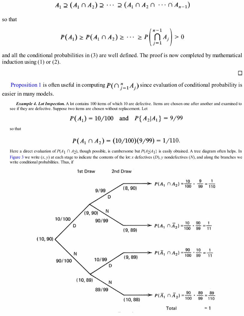
so that

and all the conditional probabilities in (3) are well defined. The proof is now completed by mathematicalinduction using (1) or (2).

Proposition 1 is often useful in computing since evaluation of conditional probability iseasier in many models.

Example 4. Lot Inspection. A lot contains 100 items of which 10 are defective. Items are chosen one after another and examined tosee if they are defective. Suppose two items are chosen without replacement. Let

so that

Here a direct evaluation of P(A1 ∩ A2), though possible, is cumbersome but P(A2|A1} is easily obtained. A tree diagram often helps. InFigure 3 we write (x, y) at each stage to indicate the contents of the lot: x defectives (D), y nondefectives (N), and along the branches wewrite conditional probabilities. Thus, if

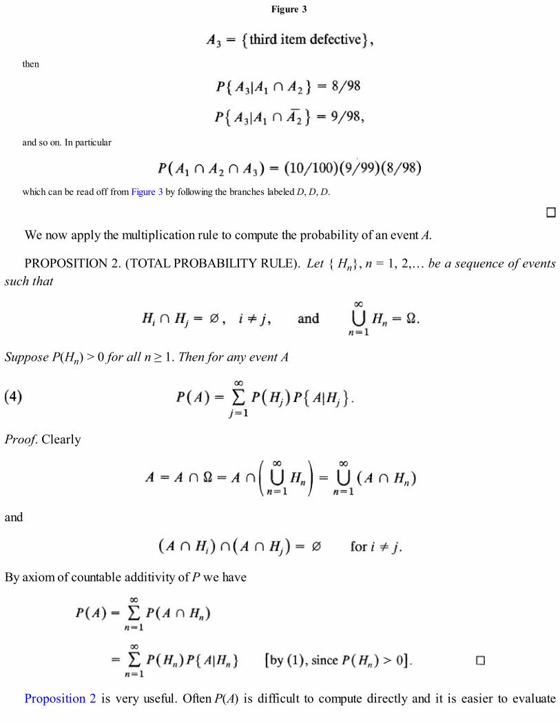
Figure 3

then

and so on. In particular

which can be read off from Figure 3 by following the branches labeled D, D, D.

We now apply the multiplication rule to compute the probability of an event A.

PROPOSITION 2. (TOTAL PROBABILITY RULE). Let { Hn}, n = 1, 2,… be a sequence of eventssuch that

Suppose P(Hn) > 0 for all n ≥ 1. Then for any event A

Proof. Clearly

and

By axiom of countable additivity of P we have

Proposition 2 is very useful. Often P(A) is difficult to compute directly and it is easier to evaluate

P(A|Hj}.

Example 5. Making a Sale. Consider a local manufacturer of mattresses who consistently runs a sales campaign in the local media.In order to evaluate the effectiveness of the campaign, the manufacturer keeps a record of whether or not a customer has seen theadvertisement and whether or not the customer makes a purchase. On the basis of this record, it is estimated that the probability that acustomer has seen their advertisement is .6, the conditional probability that a sale is completed given that the customer has seen theiradvertisement is .7, and the conditional probability that a sale is completed given that the customer has not seen their advertisement is .2.What is the probability that a randomly selected customer will make a purchase?

Let A be the event that the customer has seen their advertisement and S be the event that a customer makes a purchase. Then

A tree diagram often helps. As before, we write conditional probabilities along the branches in Figure 4. We note that the probabilitiesalong the two branches emanating from any node or vertex (such as A or ) must add to 1.

Example 6. Polya’s Urn Model. Consider an urn that contains r red and g green marbles. A marble is drawn at random and its colornoted. Then the marble, together with c > 0 marbles of the same color, are returned to the urn. Suppose n such draws are made from theurn. What is the probability of selecting a red marble at any draw?

This so-called Pólya’s urn model can be used to study the spread of epidemics. The red marbles may correspond to people in apopulation not having some contagious disease, and the green marbles to people having a certain disease.

Let Rj be the event that the j th marble drawn is red, and Gj the event that the j th marble drawn is green, j = 1, 2,…, n. It is clearthat Rj and Gj are mutually exclusive. At the k th draw there are r + g + (k – 1)c marbles in the urn, and we assume that each is equallylikely. We note that for j ≥ 2

Figure 4

and

In particular,

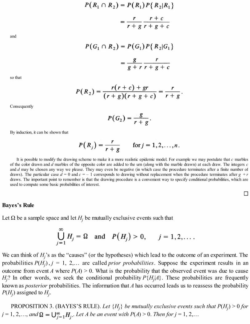
and

so that

Consequently

By induction, it can be shown that

It is possible to modify the drawing scheme to make it a more realistic epidemic model. For example we may postulate that c marblesof the color drawn and d marbles of the opposite color are added to the urn (along with the marble drawn) at each draw. The integers cand d may be chosen any way we please. They may even be negative (in which case the procedure terminates after a finite number ofdraws). The particular case d = 0 and c = – 1 corresponds to drawing without replacement when the procedure terminates after g + rdraws. The important point to remember is that the drawing procedure is a convenient way to specify conditional probabilities, which areused to compute some basic probabilities of interest.

Bayes’s Rule

Let Ω be a sample space and let Hj be mutually exclusive events such that

We can think of Hj’s as the “causes” (or the hypotheses) which lead to the outcome of an experiment. Theprobabilities P(Hj) , j = 1, 2,… are called prior probabilities. Suppose the experiment results in anoutcome from event A where P(A) > 0. What is the probability that the observed event was due to causeHj? In other words, we seek the conditional probability P{Hj|A}. These probabilities are frequentlyknown as posterior probabilities. The information that A has occurred leads us to reassess the probabilityP(Hj) assigned to Hj.

PROPOSITION 3. (BAYES’S RULE). Let {Hj} be mutually exclusive events such that P(Hj) > 0 forj = 1, 2,…, and . Let A be an event with P(A) > 0. Then for j = 1, 2,…

Proof. By definition

where we have used (4).

We need not memorize formula (5). It gives nothing new, being simply an alternative way of writingthe definition of conditional probability. In applications, we simply recreate formula (5) from thedefinition.

Example 7. Medical Diagnosis. In medical diagnosis a doctor observes that a patient has one or more of certain specified symptomsA = {S1, S2,…, Sl} and is faced with the problem of deciding which of the several possible diseases { D1, D2,…,Dk} is the mostprobable cause of the observed symptoms. Suppose it has been estimated from medical records that P(Dj) = pj, pj > 0, j = 1, 2,…,k . Weassume that the diseases never occur together in the same person. We assume further that the conditional probability P(A|Dj} can also beestimated from medical records. Then for j = 1, 2,…, k Bayes’s rule gives

which is the probability that a person with one or more symptoms A – { S1,…, Sl} has disease Dj. The most probable cause of illnessthen is the disease Dj, for which

In particular, let P(D1) = .40, P(D2) = .25, P(D3) = .35, and P{A|D1} = .8, P{A|D2} = .6, P(A|D3} = .9. Then

and

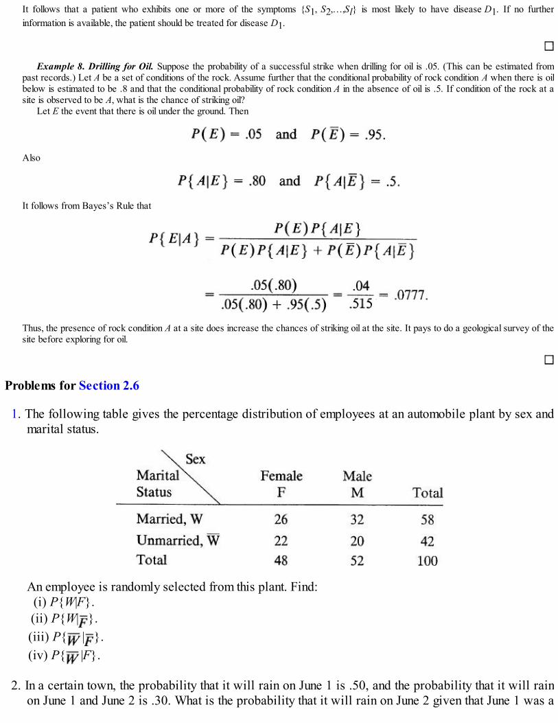
It follows that a patient who exhibits one or more of the symptoms {S1, S2,…,Sl} is most likely to have disease D1. If no furtherinformation is available, the patient should be treated for disease D1.

Example 8. Drilling for Oil. Suppose the probability of a successful strike when drilling for oil is .05. (This can be estimated frompast records.) Let A be a set of conditions of the rock. Assume further that the conditional probability of rock condition A when there is oilbelow is estimated to be .8 and that the conditional probability of rock condition A in the absence of oil is .5. If condition of the rock at asite is observed to be A, what is the chance of striking oil?

Let E the event that there is oil under the ground. Then

Also

It follows from Bayes’s Rule that

Thus, the presence of rock condition A at a site does increase the chances of striking oil at the site. It pays to do a geological survey of thesite before exploring for oil.

Problems for Section 2.6

1. The following table gives the percentage distribution of employees at an automobile plant by sex andmarital status.

An employee is randomly selected from this plant. Find:(i) P{W|F}.(ii) P{W| }.(iii) P{ | }.(iv) P{ |F}.

2. In a certain town, the probability that it will rain on June 1 is .50, and the probability that it will rainon June 1 and June 2 is .30. What is the probability that it will rain on June 2 given that June 1 was a

rainy day?

3. From a lot containing five defective and five nondefective items, a sample of five is drawn (withoutreplacement). Given that the sample contains at least three defectives, what is the probability that itcontains exactly two nondefectives?

4. A player is dealt a five-card hand from a 52-card bridge deck. A flush consists of five cards of thesame suit.

(i) Given that all the cards in the hand are black, what is the probability that the hand has a flush?(ii) Given that the hand dealt has four clubs and one card of some other suit, and the player is

allowed to discard one card in order to draw another, what is the probability that she will besuccessful in completing a flush? (Assume that she discards the card that is not a club.)

(iii) If the hand dealt has two cards that are not clubs and the player discards them to draw two newcards, what is the probability that she will complete a club flush?

5. Consider an electronic assembly with two subsystems A and B. Suppose:

Find:(i) P{A fails|B has failed}.(ii) P{A fails alone}.

6. The diameter of an electrical cable is recorded. Let Ω = [0, 1], and for any event A, P(A) = ∫A6x(1 – x)dx. Let A be the event that the diameter is ≤ 1/2, B the event that diameter is not less than 1/3 but lessthan 2/3. What is P{A|B}?

7. If 80 percent of all graduate students at a university receive some kind of financial support, and if 10percent of graduate students who are on support also work part-time, what is the probability that arandomly selected graduate student will be on support as well as working part-time?

8. Let A and B be two events such that P(A) > 0, and P(A) + P(B) > 1. Show that P{B|A} ≥ 1 – { P()/P(A)}.

9. Suppose 45 percent of the students at a university are male and 55 percent are female. If 50 percent ofthe females and 40 percent of the males smoke, what is the probability that a smoker is male?

10. Consider a lot of light bulbs that contains 30 percent of Brand A bulbs, 45 percent of Brand B bulbs,and 25 percent of Brand C bulbs. It is known that 2 percent of all Brand A bulbs, 3 percent of allBrand B bulbs, and 1 percent of all Brand C bulbs are defective. What is the probability that arandomly selected bulb from the lot will be defective?

11. Consider a bicyclist who leaves a point P (see map), choosing one of the roads PR1, PR2, PR3 atrandom. At each subsequent crossroad he again chooses a road at random.

(i) What is the probability that he will arrive at point A?(ii) What is the conditional probability that he will arrive at A via road PR3?

12. It is known from insurance records that a driver who has had a driver education program at highschool or through the American Automobile Association has an 85 percent chance of not having anaccident during the first year of driving, whereas a new driver who has not had such a program has a60 percent chance of not having an accident during the first year of driving. If 80 percent of all newdrivers undergo a driver education program,

(i) What is the probability that a new driver will finish the first year of driving without an accident?(ii) What is the probability that a new driver who is involved in an accident during the first year of

driving has had a driver education?

13. Five percent of patients suffering from a certain disease are selected to undergo a new treatment thatis believed to increase the recovery rate from 30 percent to 50 percent. A person is randomlyselected from these patients after the completion of the treatment and is found to have recovered.What is the probability that the patient received the new treatment?

14. Three identical cards, one red on both sides, one black on both sides, and the third red on one sideand black on the flip side, are placed in a box. A card is then randomly picked from the box andtossed on the table. (Assume that the color on the underside of the card is not observed.)

(i) What is the probability that the up face is red?(ii) Given that the up face is red, what is the probability that the down face is also red?

15. Four roads lead away from the county jail. A prisoner has escaped from the jail and selects a road atrandom. If road I is selected, the probability of escaping is 1/8; if road II is selected, the probabilityof success is 1/6; if road III is selected, the probability of escaping is 1/4; and if road IV is selected,the probability of success is 9/10.

(i) What is the probability that the prisoner will succeed in escaping?(ii) If the prisoner succeeds, what is the probability that the prisoner escaped by using road IV?

Road I?

16. The geographical distribution of students at a private college is given as: 50 percent from the South,10 percent from the East, 20 percent from the Midwest and 20 percent from the West. If 60 percent ofthe Easterners, 30 percent of the southerners, 10 percent of the Midwesterners, and 5 percent of theWesterners wear ties, find the probability that a student wearing a tie comes from the

(i) East.

(ii) Midwest.(iii) South.(iv) West.

17. A diagnostic test for a certain disease is 95 percent accurate in that if a person has the disease, it willdetect it with a probability of .95, and if a person does not have the disease, it will give a negativeresult with a probability of .95. Suppose only 0.5 percent of the population has the disease inquestion. A person is chosen at random from this population. The test indicates that this person hasthe disease. What is the (conditional) probability that he or she does have the disease?

2.7 INDEPENDENCE

We now consider an important special case of the multiplication rule (2.6.1) (or (2.6.2) or Proposition2.6.1) when the occurrence of an event A does not affect the assignment of probability to B. This meansthat P{ B|A} = P(B), provided P{ B|A} is well defined, that is, P(A) > 0. By multiplication rule, we seethat

We note that this relation is symmetric in A and B. We are therefore led to the following definition.

DEFINITION 1. (PAIRWISE INDEPENDENCE) . Let A and B be two events. We say that A and B are(pairwise) independent if

I f A and B are not independent, we say that they are dependent. If A and B are independent thentrivially

provided the conditional probabilities are well defined. We note that if P(A) = 0, then for any event B

so that

and A is independent of any other event.The reader needs to distinguish between independence and mutually exclusive events. Independence

is a property of probability P whereas mutual exclusion is a set theoretic property. If A and B are mutuallyexclusive events with P(A) > 0 and P(B) > 0, then P(A ∩ B) = 0 ≠ P(A)P(B) so that A and B cannot beindependent. In fact, P{A|B} = 0 = P{B|A} so that if A occurs, B cannot and if B occurs, A cannot. Thus Aand B are strongly dependent when A ∩ B = Ø.

If A and B are independent, it means that the occurrence of A does not influence the probability of B,that is, one cannot say anything about the occurrence of B from the knowledge that A has occurred.

Therefore, if A and B are independent, so should be A and and, by symmetry, and B, and and .We leave the reader to prove the following result.

PROPOSITION 1. Two events A and B are independent if and only if

(i) A and are independent, or(ii) and B are independent, or(iii) and are independent.

In practice, it is often easy to conclude from physical consideration of the experiment whether or nottwo events are independent, but the only way to be sure is to check that (1) holds.

Example 1. Sampling With Replacement. A lot contains 1000 items of which five are defective. Two items are randomly drawn asfollows. The first item drawn is tested and replaced in the lot before the second item is selected. Let Ai be the event that i th item drawnis defective, i = 1, 2. Then A1 and A2 are independent events and

On the other hand, if the first item is not replaced in the lot than A1 and A2 are dependent events. Moreover,

Example 2. Families with Two Children. Consider families with two children and assume that the four possible sex distributions bb,bg, gb, gg are equally likely. Let A be the event that a randomly selected family has children of both sexes and B the event that the familyhas at most one girl. Then

It follows that A and B are dependent. This is by no means obvious from the experiment.Indeed, if we consider families with three children, then

so that

and A and B are independent. Thus it is not always obvious whether or not two events A and B are independent.

Example 3. System Reliability. Consider a system that has two components or subsystems connected in series, as shown in Figure1. The system functions if and only if both the components C1 and C2 are operational. If the two components operate independently thenthe reliability of the system as measured by the probability that it will survive to time t is given by

If in Example 3 we have more than two components in the system, how do we go about computing system reliability? Clearly, weneed to extend the concept of independence to more than two events. Suppose we have three events A, B, and C. If they are pairwiseindependent, then

Is the requirement (2) enough to say A, B, and C are independent? If not, it does not help us solve the problem of Example 3 with threecomponents. For that purpose we need to say something about P(A ∩ B ∩ C). Suppose we require that

It turns out that (3) does not imply (2) and (2) does not imply (3), so we must require both. We are led to the following definition.

DEFINITION 2. (MUTUAL INDEPENDENCE). The n events A1, A2,…, An are mutually independent if the following 2n – n – 1relations hold:

Figure 1. System in series.

Example 4. Examples where (2) (3) and (3) (2). Suppose four identical slips of cards marked aaa, abb, bab, bbarespectively are placed in a box. The contents of the box are well shuffled and a card is drawn at random. Define the events

Then P(A) = P(B) = P(C) = 1/2,

so that A, B, C are pairwise independent. Since, however,

A, B, C are not mutually independent. Thus (2) (3).We next consider an example where (3) (2). Suppose a pair of fair dice is rolled so that

Let

It is clear that A, B, and C are not independent. In fact A, B and B, C and C, A are pairwise dependent. However,

Fortunately, it is not very often that we need to check that given events A1, A2,…, An are independent.Often it will be a part of our hypothesis or will follow from the manner in which the experiment is set up(see page 61). In that case we can use the multiplication rule for independent events

for any subset Ai1, Ai2,…, Aik of A1, A2,…, An.

Example 5. System Reliability. Consider a system with k subsystems connected in series (Example 3). The system operatessuccessfully if and only if all the subsystems operate successfully. We assume that the subsystems operate independently.

Let A be the event that the system operates successfully and Ai, the event that the i th subsystem operates successfully. Then thereliability of A is given by

since Ai’s are independent. In particular, if k = 5 and P(Ai) = .95 for each i, then

Next we consider a system connected in parallel (as shown in Figure 2). The system operates successfully if and only if at least oneof the subsystems successfully operates. It follows that so that the reliability of A is given by

In order to use the independence of Ai we write:

Figure 2. System in parallel.

In particular, if k = 5, and P(Ai) = .90 for each i, then

Independent TrialsRecall that events A and B are independent if and only if P(A ∩ B) = P(A)P(B). We emphasize that formore than two events to be independent, it is not enough to check pairwise independence. We have toshow that the multiplication rule holds for every pair, every triple, and so on.

We now wish to make precise what we mean by “independent repetitions of an experiment” that wasused in Section 2.3 [see (2.3.1) and the following footnote].

For convenience, any performance of an experiment is referred to as a trial. If the same experiment isrepeated n times we speak of n trials of the experiment.

Suppose we perform n experiments with respective sample spaces Ω1, Ω2,…, Ωn. We can think of then experiments as a single combined experiment with sample space Ω where† Ω consists of outcomes ( ω,ω2,…,ωn) with ωi ∈ Ωi, i = 1, 2,…,n. This means that the first experiment results in outcome ω1, thesecond in outcome ω2, and so on. We require further that if Ai is an event in Ωi, then {(ω1, ω2,…, ωn)} ∈Ω, ωi ∈ Ai} is an event in Ω.

DEFINITION 3. The n experiments with sample spaces Ω1, Ω2,…, Ωn are said to be independent ifany events A1, A2,…, An whatever with Ai ⊆ Ωi, i = 1, 2,…, n are (mutually) independent (in the sense ofDefinition 2),

According to Definition 3, the probability of any event in any sample space Ωi, is unaffected by whathappens in any other sample space Ωj(i ≠ j). We emphasize that we say nothing in Definition 3 aboutevents in the same sample space. Thus if Ai, Bi are events in Ωi, they may or may not be independent. Butany event Bi in Ωi, is independent of Aj or Bj in Ωj, and so on.

Example 6. Tossing a Coin and Rolling a Die. A fair die is rolled and a fair coin is tossed independently. Then we have twoexperiments with

On Ω1 we assign uniform probability P{i} = 1/6 for i = 1, 2,…, 6, and on Ω2 also we assign uniform probability P{H } = P{T} = 1/2. Thecombined experiment has sample space

where we assign the equal probabilities

Let A = {even face value on die} ⊆ Ω1, and B = {heads on the coin} ⊆ Ω2. Then A and B are independent. However, if C = {odd facevalue on die} ⊆ Ω1, then A and C are dependent but C and B are independent.

The case of most interest in statistics is the case when Ω1 = Ω2 = ··· = Ωn. That is, when the sameexperiment is repeated n times. If the repetitions are independent in the sense of Definition 3, we speak ofn independent trials of the experiment (with sample space Ω1). In practice it may almost be impossible tocheck that a model with independent trials is appropriate. Fortunately, we do not have to do so if we arecareful enough to set up the experiment in such a way that there is no interaction between the trials. Given,however, that the trials are independent, we can always use the multiplication rule on the combinedsample space Ω.

Example 7. Coin Tossing. A coin is tossed 20 (independent) times. Each toss is considered a trial. Since the trials are independent,the probability that 20 trials produce 20 heads is p20, where p = P (heads on any trial), 0 < p < 1.

Suppose a coin is tossed 10 times and 9 heads are observed. Is there evidence to suggest that the coin is biased? If the coin were fair,

the probability of observing 9 heads in 10 tosses is . (We choose 9 trials for 9 heads out of 10 trials in ways and

each of these sequences of 9 heads and one tail, by independence, has the same chance .) This probability is small ( = .0098).Note that if we were to reject the claim that the coin is fair when we observe 9 heads in 10 trials, we will certainly do so when weobserve all 10 heads. Hence the event of interest is not “exactly 9 heads” but “at least nine heads.” The probability of this event is

Thus in a large number of sequences of 10 trials with a fair coin, about 1 percent of the trials will produce at least 9 heads. We can hardlydismiss 9 heads on 10 trials as a mere coincidence, and we have to conclude that the coin is not fair.

Example 8. Tossing a Pair of Fair Coins. A pair of fair coins is tossed n (independent) times. Each trial has sample space Ω1 ={HH, HT, TH, TT} on which we assign uniform probability P{ ω } = 1/4, ω ∈ Ω1. Let A = {exactly one head}, B = {at least one head}.On any given trial, say trial 1, A and B are dependent events since P(A) = 1/2, P(B) = 3/4 and P(A ∩ B) = 2/4 ≠ P(A)P(B). But event A ontrial 1 is independent of event B on trial 2 or of event A on trial 2, and so on. Thus

Example 9. Drug Testing. A doctor studying cures for a certain disease tries a new drug on n randomly selected patients sufferingfrom the disease. In this case the administration of the drug to each patient may be considered a trial. It is reasonable to assume that thetrials are independent since the probability that the first patient is cured does not affect (and is not affected by) the probability that thesecond patient is cured, and so on.

Suppose that the doctor tries the new drug on eight patients and finds that seven patients are cured. It is known that the traditionaltreatment is only 40 percent effective. Is there evidence to suggest that the new drug is more effective? If the new drug is not effective,than the probability of success is .4. Under this assumption, the probability that 7 or more patients will be cured by the new drug is

(The argument used here is the same as in Example 7.) Since it is highly improbable to get seven or more cured out of eight patients withthe traditional treatment, we have to conclude that our assumption that the probability of success with new drug is .4 is not reasonable. Itdoes not mean that our assumption is necessarily false but only that it is more reasonable to conclude that the new drug is more effectivethan the one presently in use.

Example 10. Quality Control. To keep control on the quality of flash bulbs that a company produces, n randomly selected bulbs areinspected from a day’s production. Each inspection is considered a trial. Since the probability that the first bulb, say, is defective does notaffect the probability that the i th bulb (1 ≤ i ≤ n) is defective, and so on, it is reasonable to postulate that the trials are independent.

Problems for Section 2.7

1. Which of the following pairs of events are independent?(i) Smoking and lung cancer.(ii) Rain on a particular day and rain on the day following the first.(iii) Drinking alcohol and having a car accident.(iv) High-school grades and college performance.(v) Winning a state lottery and buying a car.(vi) Being a male and having blue eyes.(vii) Being a girl and playing baseball.(viii) Being six feet tall and weighing over 160 pounds.

2. Which of the following pairs of events are mutually exclusive?(i) Being under 20 and earning $20,000 year,(ii) Being a college student and owning a car.(iii) Rolling ones on two successive rolls of a die.(iv) Rolling a sum of 6 or a sum of 12 with a pair of dice.(v) Rolling an odd face value and rolling an even face value on a single roll of a die.

3. A fair die is rolled twice. Let A1, A2, A3 be the events

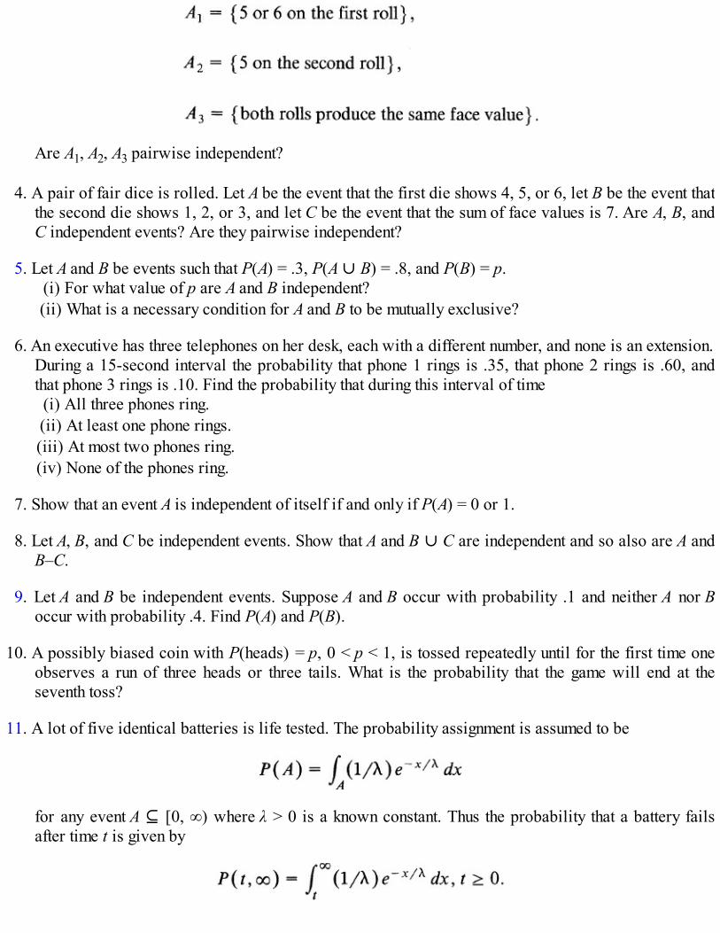
Are A1, A2, A3 pairwise independent?

4. A pair of fair dice is rolled. Let A be the event that the first die shows 4, 5, or 6, let B be the event thatthe second die shows 1, 2, or 3, and let C be the event that the sum of face values is 7. Are A, B, andC independent events? Are they pairwise independent?

5. Let A and B be events such that P(A) = .3, P(A ∪ B) = .8, and P(B) = p.(i) For what value of p are A and B independent?(ii) What is a necessary condition for A and B to be mutually exclusive?

6. An executive has three telephones on her desk, each with a different number, and none is an extension.During a 15-second interval the probability that phone 1 rings is .35, that phone 2 rings is .60, andthat phone 3 rings is .10. Find the probability that during this interval of time

(i) All three phones ring.(ii) At least one phone rings.(iii) At most two phones ring.(iv) None of the phones ring.

7. Show that an event A is independent of itself if and only if P(A) = 0 or 1.

8. Let A, B, and C be independent events. Show that A and B ∪ C are independent and so also are A andB–C.

9. Let A and B be independent events. Suppose A and B occur with probability .1 and neither A nor Boccur with probability .4. Find P(A) and P(B).

10. A possibly biased coin with P(heads) = p, 0 < p < 1, is tossed repeatedly until for the first time oneobserves a run of three heads or three tails. What is the probability that the game will end at theseventh toss?

11. A lot of five identical batteries is life tested. The probability assignment is assumed to be

for any event A ⊆ [0, ∞) where λ > 0 is a known constant. Thus the probability that a battery failsafter time t is given by

If the times to failure of the batteries are independent, what is the probability that at least one battery willbe operating after t0 hours?

12. On Ω = (a, b), – ∞ < a < b < ∞, each subinterval is assigned a probability proportional to the lengthof the interval. Find a necessary and sufficient condition for two events to be independent.

13. It is estimated that the percentages of A, B, O, and AB blood types in a certain population are,respectively, 40, 20, 30, and 10. Three individuals are picked (independently) from this population.(Assume that the population is very large.) Find the probability that:

(i) They are all type AB.(ii) They are all of the same blood type.(iii) They are all different blood types.(iv) At least two are blood type A.(v) None is blood type A.

14. In the World Series of baseball, two teams play a sequence of 4 to 7 games. The first team to win 4games wins the Series, and no further games are played. If the two teams are evenly matched and theoutcomes of different games are independent, find the probability that the series will terminate at theend of:

(i) The fourth game.(ii) The fifth game.(iii) The sixth game.(iv) The seventh game.

15. A process is in control if it produces at most 5 percent defectives. Random samples of 20 items aretaken periodically, and if the sample contains at least two defectives, the process is stopped. What isthe probability that the process will be stopped when in fact it is producing only 5 percentdefectives?

16. In People vs. Collins, an elderly woman was assaulted from behind and robbed on June 18, 1964 inLos Angeles. The victim claimed that she saw a young blond woman run from the scene. Anotherwitness said that he saw a Caucasian woman with dark blond hair and ponytail run out of the alleyand enter a yellow automobile driven by a black male with mustache and beard. Within a few days ofthe crime an interracial couple, Janet and Malcolm Collins, was arrested on the strength of thesedescriptions and charged with the crime. At the trial a mathematician using the product rule forindependent events with probabilities

Event ProbabilityA. Yellow car .10B. Man with mustache .25C. Woman with ponytail .10D. Woman with blond hair .33E. Black man with beard .10F. Interracial couple in a car .001

testified that the chance was 1 in 12 million that a couple selected at random would possess these

characteristics. The probability was overwhelming, he argued, that the accused were guilty becausethey matched the unusual description. The jury convicted. Do you agree with the mathematician’scalculations and conclusion? If not, why not? (On appeal the conviction was reversed. The SupremeCourt of California ruled that the trial court should not have admitted the probabilistic evidence.)

17*. In People vs. Collins of Problem 16, the court computed the conditional probability that at least oneother couple exists matching these characteristics, given that at least one such couple exists, as

where p is the probability of selecting at random a couple with the characteristics of the accused andN is the total number of couples in the area. Derive this result. Letting p = 1/N and N → ∞ show thatthis conditional probability approaches (e – 2)/(e – 1) .418. (The court argued that even if oneaccepts the prosecution’s figures that p = 1/12,000,000, the probability is .42 that the coupleobserved by the witnesses could be duplicated by at least one other couple with the samecharacteristics.)

18*. A game of craps is played with a pair of fair dice as follows. A player rolls the dice. If a sum of 7 or11 shows up, the player wins; if a sum of 2, 3, or 12 shows up, the player loses. Otherwise the playercontinues to roll the pair of dice until the sum is either 7 or the first number rolled. In the former casethe player loses and in the latter the player wins.

(i) Find the probability that the player wins on the n th roll.(ii) Find the probability that the player wins the game.(iii) What is the probability that the game ends on:

(a) The first roll?(b) Second roll?(c) Third roll?

19. Consider a pair of fair dice, A and B. Die A is tossed once. If the face value is i, i ∈ {1, 2, 3, 4, 5, 6},then die B is tossed i times and the sum of the face values on the i tosses of die B is taken.

(i) Find the probability that the sum is 6.(ii) Find the probability that die B was rolled j times (j = 1, 2, 3, 4, 5, 6) given that the sum of face

values is 6.

Figure 3a

Figure 3b

Figure 3c

Figure 4

(iii) Suppose die A is loaded in such a way that P{i} = pi > 0, i = 1, 2,…, 6, and die Bis fair. Find the probabilities in parts (i) and (ii) above.

(iv) Suppose die A is fair but die B is loaded with P{i} = qi > 0, . Repeat parts (i) and(ii).

20. Consider five relays connected as shown in Figures 3a, 3b and 3c. A message will be transmittedfrom Terminal A to Terminal B: if the relays R 1 to R5 in Figure 3a are all closed; if the relays R1 toR3 or R4 and R5 in Figure 3b are closed; if at least one of the relays R1, R2,…, R5 in Figure 3c isclosed. Suppose all the relays function independently and have the same probability .8 of beingclosed. Find the probability (in each case) that the message will be transmitted.

21. Consider two parallel systems connected in a series as in Figure 4. Assuming that all the fourcomponents operate independently and that the probability that a C-type component functions is p1while that for a D-type component is p2, what is the reliability of the system?

2.8 SIMPLE RANDOM SAMPLING FROM A FINITE POPULATION

The reader has no doubt heard the phrase “random sample” as applied to samples taken by the Gallup andHarris organizations. For the Gallup poll, for example, a sample of size of about 1500 is taken from theentire voting age population of citizens of the United States. How can one make inferences about theelection results, for example, on the basis of such a small sample?

We recall that a population is a group of objects about which some information is desired. Thus wespeak of the population of voting age citizens of a country, the population of heights of entering freshman,the population of family incomes in a city, and so on. A sample is a part of the population under study, andthe objective in statistics is to make inferences about the population from the sample. For example, onemay be interested in the proportion of eligible voters who are registered to vote or in the average age ofall eligible voters. Clearly no amount of sampling is going to lead to conclusions that are 100 percentaccurate unless the sample consists of the entire population, that is, unless we take a census. A census,however, is frightfully expensive and time-consuming. Moreover, in many instances (for example, in lifetesting of batteries) the items in the sample are destroyed. If an automobile manufacturer has to test-driveevery car it produces in order to report the average miles per gallon of gasoline that its cars give, thenthere will be nothing to sell. A carefully chosen sample, on the other hand, can give fairly reliable results.It is clear that not just any sample will do if we have to make probability statements about our inferences.For example, if you were the buyer for a large department store, you would not just look at a couple ofshirts from the top of a box. You would do well to sample each box in order to evaluate the quality of theshipment. The two shirts on top may not be representative of the entire box. The ones at the bottom, forexample, may be irregular.

In statistics we take probability samples, that is, some random or probability device is used in theselection process. This allows us to evaluate the performance of our procedure.

The simplest form of a probability sample is called a simple random sample.

DEFINITION 1. (SIMPLE RANDOM SAMPLE). A simple random sample of size n from a populationof N objects is a sample chosen in such a way that every collection of n objects in the population has thesame chance of being selected.

We note that there are Nn different ordered samples of size n from a population of N objects ifsamples are taken with replacement and NPn ordered samples if sampling is done without replacement. Insampling without replacement and without regard to order, there are samples of size n. It follows that

in simple random sampling all possible samples have the same chance, namely, 1/Nn in ordered samplingwith replacement and 1/NPn in ordered sampling without replacement. Similarly, in unordered, without-

replacement sampling, each sample has probability 1/ of being selected. For large N and small n/N,

the ratio NPn/Nn is close to one, so that for large populations (and relatively small-sized samples) weexpect the two methods of sampling to be equivalent for all practical purposes.

Typical examples of random sampling with replacement are coin tossing and die rolling. Randomsampling without replacement occurs typically in lotteries, successive drawing of cards from a deck, andopinion surveys.

In this section we consider only the case when the population is finite and sampling is done withoutreplacement (and without regard to order). The case when the population is infinite and also its specialcase when the population is finite and sampling is done with replacement will be considered in Section3.8.

How do we go about taking a simple random sample? (Unless otherwise stated, we will assume thatall samples are simple random samples and we will drop the adjective “simple” from here on.) In theorytaking, a random sample is equivalent to drawing n marbles from an urn that contains N marbles, eachcorresponding to one and only one element of the population. In practice, this is hardly, if ever, done. Oneuses, instead, a table of random numbers (such as Table A1 in the Appendix). A table of random numbersis a list of ten digits 0, 1, 2,…, 9 with the following properties.

(i) The digit in any position in the list has the same chance, namely 1/10 of being 0, or 1, or 2,…, or9.

(ii) The digits in different positions are independent.

The random digits are arranged in groups of five into numbered rows in order to facilitate the use of thetable. In view of (i) and (ii), we note that any pair of digits in the table has the same chance, namely1/100, of being 00, or 01, or 02,…, or 99; in general, any k-tuple of digits in the table has the samechance, namely, 1/10k of being 00…0, or 00…01, or 00…02,…, or 99…9.

In order to use Table Al, we take the following steps.

(i) Find the number of digits in N – 1 where N is the population size.(ii) Label (in any manner whatever) the N elements in the population from 0…0 to N – 1 where each

label has the same number of digits as N – 1.(iii) Enter Table Al in any place whatever, and systematically read through the table either across or

down in groups of k where k is the number of digits in N – 1.(iv) Choose as many k-digit numbers that are less than or equal to N – 1 as desired. (We drop

duplicates of random numbers already selected.)

Example 1. Random Sample of Voters. A random sample of 10 voters is to be taken from a voters list consisting of 4832 names.Since N – 1 = 4831 has four digits we look for four-digit random numbers from 0000 to 4831. For example, entering Table A1 on line 21and reading across, we get the random numbers

If we agree to take only the first four digits of each five-digit group, and we take only the numbers less than or equal to 4831, then oursample consists of voters labeled

We leave the reader to show that each of 4832 voters has the same probability 1/4832 of being included in the sample.

Example 2. Choosing Five of the Fifty States. Suppose a random sample of five is to be taken from 50 states of the United States.Let us list the states alphabetically and number them from 00 for Alabama to 49 for Wyoming. Suppose we begin with the

42nd row of Table A1. We get the following two-digit numbers:

Ignoring numbers above 49 and duplicates, we obtain the following five distinct numbers,

which correspond to Idaho, Ohio, Missouri, Texas, and Illinois. This is our random sample of five states.

Remark 1. It is customary to use a different page and a different line of Table A1 for each application.This can be done by some random procedure.

Remark 2. A random sample is used to represent the population. One cannot simply look at a sampleand determine whether the sample resembles the population or not. All one can do is to examine themethod used in selecting the sample. If, for example, the method used systematically excludes someelements of the population, the selection procedure is biased. It is therefore important to ascertain how thesample was chosen.

Remark 3. Simple random sampling is not the only method of obtaining probability samples. Otherprobability samples such as stratified random samples or cluster samples are often used and may bemore efficient. (A stratified random sample divides the population into several strata. Simple randomsamples are then taken from each strata. The combined sample is called a stratified random sample. Incluster sampling, groups of elements are chosen randomly.) The Gallup election year poll, for example,uses a multistage cluster sample rather than a simple random sample. The country is divided into fourgeographical regions: Northeast, South, Midwest, and West. Within each region, all population centers ofsimilar size are grouped together and in the first stage, simple random sample of these towns is selected.Each town is divided into wards, which are further subdivided into precincts. At the second stage, arandom sample of wards is selected. A simple random sample of precincts is selected at the third stage,from the selected wards. The fourth stage consists of drawing a simple random sample of householdsfrom the selected precincts. Finally, some members of the households selected are interviewed.

Figure 1

TABLE 1. Sample Sizes for Prescribed Levels of Confidence and Margins of Error (in SimpleRandom Sampling)

Remark 4. (Sample Size). We have not yet answered the question that is most often asked aboutsampling, or more specifically, about public opinion polls. How does a sample of 1500 to 1800 votersfrom a population of 135 million eligible voters allow us to make such accurate predictions? The firstpoint to remember is that no sample short of a census will produce results that are 100 percent accurate.The object, therefore, is to come as close as possible to 100 percent accuracy. We now need to make twochoices. First, how accurate do we want to be in our predictions? The level of accuracy desired (knownas confidence level) is usually taken to be large (90, 95 or 99 percent). The second choice, given the first,is that of the margin of error. Within how many percentage points of the true figure do we want to be? Insample surveys the margin of error is usually taken to be between 3 to 5 percent. The size of the sampledepends on these two choices and not on the population size (provided the population size is large andthe sample size is relatively small). In particular, this means that pretty much the same sample size will berequired whether the population consists of 150 million people or 500,000 people, provided theconfidence level and the margin of error desired are the same. The second point to remember is that insimple random sampling the margin of error for a given confidence level is proportional to 1/ and not1/n where n is the sample size. This means that a doubling of the sample size does not halve the margin oferror. Since even sample sizes of 1 or 2 million will produce a certain (however small) margin of error,the time and cost considerations demand that we choose as small a sample as is consistent with ourrequirements. Most surveys determine the sample size that gives a margin of error of 3 to 5 percent with95 percent accuracy. If p is the true proportion of voters in a population favoring candidate X (p will notbe known and we need to make a guess at it), then the following table gives the sample size required insimple random sampling for several selected levels of confidence and margins of errors associated withthe sample proportion favoring X as an estimate or guess of p.

The various concepts such as confidence level, margin of error, and the procedure to determinesample size will all be discussed in detail in later chapters. In particular, see Chapter 4 and Example9.6.3.

Remark 5. Having settled the question of sample size, how can a sample survey be so accurate?Probability samples are representative of the population being sampled. The situation is similar to bloodtesting where we take a few drops of blood as representative of the condition of the blood of a person.People show much more variation; nevertheless, as a totality they do conform to certain patterns ofbehavior. If, therefore, a sample is broadly representative of the population being sampled, we should getfairly reliable results. This is accomplished by probability samples.

Problems for Section 2.8

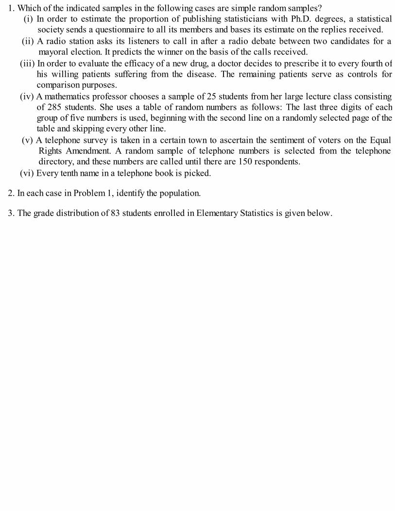
1. Which of the indicated samples in the following cases are simple random samples?(i) In order to estimate the proportion of publishing statisticians with Ph.D. degrees, a statistical

society sends a questionnaire to all its members and bases its estimate on the replies received.(ii) A radio station asks its listeners to call in after a radio debate between two candidates for a

mayoral election. It predicts the winner on the basis of the calls received.(iii) In order to evaluate the efficacy of a new drug, a doctor decides to prescribe it to every fourth of

his willing patients suffering from the disease. The remaining patients serve as controls forcomparison purposes.

(iv) A mathematics professor chooses a sample of 25 students from her large lecture class consistingof 285 students. She uses a table of random numbers as follows: The last three digits of eachgroup of five numbers is used, beginning with the second line on a randomly selected page of thetable and skipping every other line.

(v) A telephone survey is taken in a certain town to ascertain the sentiment of voters on the EqualRights Amendment. A random sample of telephone numbers is selected from the telephonedirectory, and these numbers are called until there are 150 respondents.

(vi) Every tenth name in a telephone book is picked.

2. In each case in Problem 1, identify the population.

3. The grade distribution of 83 students enrolled in Elementary Statistics is given below.

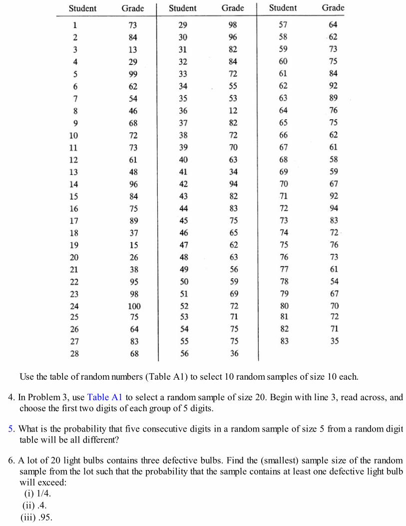
Use the table of random numbers (Table A1) to select 10 random samples of size 10 each.

4. In Problem 3, use Table A1 to select a random sample of size 20. Begin with line 3, read across, andchoose the first two digits of each group of 5 digits.

5. What is the probability that five consecutive digits in a random sample of size 5 from a random digittable will be all different?

6. A lot of 20 light bulbs contains three defective bulbs. Find the (smallest) sample size of the randomsample from the lot such that the probability that the sample contains at least one defective light bulbwill exceed:(i) 1/4.(ii) .4.(iii) .95.

7. A class has five sophomores, three juniors, and two seniors.(i) What is the smallest sample size required so that with a probability of at least .6 the sample will

contain all three juniors?(ii) What is the smallest sample size needed so that with probability at least .45 the sample will

contain all three juniors and both seniors?

8. From a population of N elements a random sample of size n is taken. Show that(i) in without-replacement sample, the probability that any fixed element of the population will be

included in the random sample is n/N, (n < N).(ii) In with-replacement sampling the corresponding probability is 1 – {(N – 1)/N}n.

9. In 1936, Literary Digest magazine predicted an overwhelming victory (by a margin of 57 percent to43 percent) for Landon over Roosevelt. This prediction was based on a mail-in poll conducted by themagazine. It mailed out 10 million questionnaires of which 2.4 million were returned. These namescame from the club’s membership roster, from telephone books, and from other lists. However,Roosevelt won the election by 62 percent to 38 percent. Where did the magazine go wrong in itsprediction? (The same year Gallup predicted with a sample of only 3000 what the Literary Digest’spredictions were going to be. Moreover, with another sample of 50, 000 people Gallup was able topredict correctly that Roosevelt would win, although he forecast that the margin would be 56 percentfor Roosevelt to 44 percent for Landon.)

10. In the 1948 election three independent polls (Gallup, Crossley, and Roper) predicted well ahead ofthe election that Dewey would win over Truman by a margin of about 5 percent. In the election,however, Truman won over Dewey by a margin of about 5 percent. The method used by threepollsters is called quota sampling. In quota sampling, each interviewer has a fixed quota of subjectsto interview. Moreover, the number of subjects falling into certain categories such as sex, age, race,and economic status are also fixed. The interviewer was free to select anyone he or she wished to.What went wrong?

11. Before the 1980 presidential election, Jimmy Carter and Ronald Reagan had a televised debate, onOctober 28. The ABC Television network announced that it would conduct a poll of viewersimmediately following the debate. Viewers were asked to call in one of two special telephonenumbers, one for those favoring Carter and the other for those favoring Reagan. The viewers weretold that their local telephone company would bill them 50 cents for the call. The results werereported by ABC News later that night. Callers favored Reagan over Carter by a 2–1 margin. Thepoll was roundly criticized by the media and experts. Why?(About 736,000 calls were received by 12:53 a.m. of October 29, when the ABC poll closed. At anytime until then, about 5,000 calls could be received by either number. In the 1980 election Reaganwon over Carter by a huge margin.)

2.9 REVIEW PROBLEMS

1. Let f be as defined below, and define P by P(A) = ∫Af(x) dx where A is an event. Does P define aprobability?(i) f(x) = (x + θ/2)/θ2, 0 ≤ x ≤ θ, and zero elsewhere.(ii) f(x) = 3x2/2θ3 if 0 ≤ x ≤ θ, = 3(x – 2θ)2/2θ3 if θ ≤ x ≤ 2θ, and zero elsewhere.

(iii) f(x) = 3(θ + x)2/2θ3 for – θ ≤ x ≤ 0, = 3(θ – x)2/2θ3 for 0 ≤ x ≤ θ, and zero elsewhere.(iv) f(x) = 1/x2, x ≥ 1, and zero elsewhere.(v) f(x) = θeθx, x < 0, and zero elsewhere.

In each case where the answer is yes, find P(A) where A = ( – 1, 1).

2. Let Ω = {0, 1, 2,… }. For A ⊆ Ω, define P(A) as follows:(i) P(A) = 1 if A contains the element 0 and P(A) = 0 otherwise.

(ii) P(A) = λ > 0, 0 < p < 1 are constants.

Does P define a probability?

3. Let A, B, and C be three events, and suppose that A ∩ B ⊆ C. Show that P( ) ≤ P( ) + P( ).

4. The Supreme Court of the United States has nine Justices (a Chief Justice and eight AssociateJustices). Suppose all Justices vote randomly (for or against) on a particular issue before the Court.(i) Find the probability that a majority votes in favor of the plaintiff.(ii) If a specified judge abstains, find the probability of a tied vote.(iii) If there are four women and five men Justices, find the probability that they vote along sex lines.

(A unanimous vote on the issue may be excluded.)

5. Suppose n books numbered 1 through n are arranged in a random order on a shelf. What is theprobability that books numbered 1, 2,…, r (r < n) appear as neighbors in that order?

6. A movie theatre can accommodate n + k people. Suppose n seats are occupied. Find the probabilitythat r( ≤ n) given seats are occupied.

7. Let A and B be two independent events such that P(A) > 0, P(B) > 0. For any event C show thatP{C|A} = P(B)P{C|A ω B} + P{ )P{C|A ∩ }.

8. In a multiple choice test with k choices to each question, a candidate either knows the answer withprobability p, 0 ≤ p ≤ 1, or does not know the answer with probability 1 – p. If he knows the answer,he puts down the correct answer with probability .9, whereas if he guesses, the probability of hisguessing correctly is 1/k. Find the conditional probability that the candidate knew the answer to aquestion, given that he has answered the question correctly. Show that this probability tends to 1 as k→ ∞.

9. A biased coin with probability p, 0 < p < 1, of heads is tossed until a head appears for the first time.What is the probability that the number of tosses required is even? Odd?

10. A pond contains red and golden fish. There are 3000 red and 7000 golden fish, of which respectively200 and 500 are tagged.(i) Find the probability that a random sample of 100 red and 200 golden fish will show 15 and 20

tagged fish respectively.(ii) Find the probability that a random sample of 300 fish will show 15 red tagged and 20 green

tagged fish.

11. In Problem 2.3.8 we considered a person who has six keys in her key chain, only one of which fits the

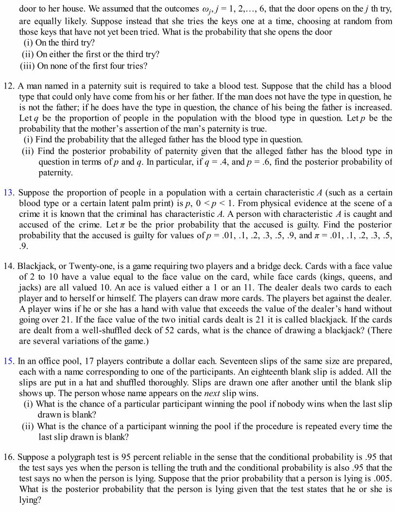
door to her house. We assumed that the outcomes ωj, j = 1, 2,…, 6, that the door opens on the j th try,are equally likely. Suppose instead that she tries the keys one at a time, choosing at random fromthose keys that have not yet been tried. What is the probability that she opens the door

(i) On the third try?(ii) On either the first or the third try?(iii) On none of the first four tries?

12. A man named in a paternity suit is required to take a blood test. Suppose that the child has a bloodtype that could only have come from his or her father. If the man does not have the type in question, heis not the father; if he does have the type in question, the chance of his being the father is increased.Let q be the proportion of people in the population with the blood type in question. Let p be theprobability that the mother’s assertion of the man’s paternity is true.

(i) Find the probability that the alleged father has the blood type in question.(ii) Find the posterior probability of paternity given that the alleged father has the blood type in

question in terms of p and q. In particular, if q = .4, and p = .6, find the posterior probability ofpaternity.

13. Suppose the proportion of people in a population with a certain characteristic A (such as a certainblood type or a certain latent palm print) is p, 0 < p < 1. From physical evidence at the scene of acrime it is known that the criminal has characteristic A. A person with characteristic A is caught andaccused of the crime. Let π be the prior probability that the accused is guilty. Find the posteriorprobability that the accused is guilty for values of p = .01, .1, .2, .3, .5, .9, and π = .01, .1, .2, .3, .5,.9.

14. Blackjack, or Twenty-one, is a game requiring two players and a bridge deck. Cards with a face valueof 2 to 10 have a value equal to the face value on the card, while face cards (kings, queens, andjacks) are all valued 10. An ace is valued either a 1 or an 11. The dealer deals two cards to eachplayer and to herself or himself. The players can draw more cards. The players bet against the dealer.A player wins if he or she has a hand with value that exceeds the value of the dealer’s hand withoutgoing over 21. If the face value of the two initial cards dealt is 21 it is called blackjack. If the cardsare dealt from a well-shuffled deck of 52 cards, what is the chance of drawing a blackjack? (Thereare several variations of the game.)

15. In an office pool, 17 players contribute a dollar each. Seventeen slips of the same size are prepared,each with a name corresponding to one of the participants. An eighteenth blank slip is added. All theslips are put in a hat and shuffled thoroughly. Slips are drawn one after another until the blank slipshows up. The person whose name appears on the next slip wins.

(i) What is the chance of a particular participant winning the pool if nobody wins when the last slipdrawn is blank?

(ii) What is the chance of a participant winning the pool if the procedure is repeated every time thelast slip drawn is blank?

16. Suppose a polygraph test is 95 percent reliable in the sense that the conditional probability is .95 thatthe test says yes when the person is telling the truth and the conditional probability is also .95 that thetest says no when the person is lying. Suppose that the prior probability that a person is lying is .005.What is the posterior probability that the person is lying given that the test states that he or she islying?

17. Let A1, A2,…, An be n events. We have seen in Corollary 2 to Proposition 2.4.3 how to compute , given P(Ai), P(Ai ∩ Aj), P(Ai ω Aj ∩ Ak),…, and so on. Show that the following bounds

hold:

where the inequality changes direction each time we add an additional term in the expansion of .

In particular, let:

Find the best possible bounds for P(A1 ∪ A2 ∪ A3 ∪ A4).

18. An Elementary Statistics course has 123 students, numbered 1 to 123. Select a random sample of size23 as follows. Begin with line 24 of Table A1, selecting the first three digits of each group of five-digit numbers.

19. Suppose A and B are independent events with P(A) = 1/4 and P(B) = 3/4. Find:(i) P(A ∪ B),(ii) P{A|A ∪ B}.

(iii) P{B|A ∪ B}.

20. Suppose current flows through three switches A1, A2, and A3 to a heater and back to the battery asshown in the diagram. Suppose further that the switches operate independently and the probabilitythat switch A1 is on (closed) is .9, that switch A2 is on is .8, and that switch A3 is on is .85. Find theprobability that the heater is on.

21. A nuclear power plant has a fail-safe mechanism that consists of eight protective devices A1, A2,…, A8which operate independently. An accident will take place if at least seven devices fail. Suppose theprobability that any single device fails is .1. Find the probability of an accident. Find the probabilitythat at least five out of the eight devices fail.

22. Two mechanics working for the same company have the same type of citizen band equipment in theirvans. The range of their system is 30 miles. Mechanic A traveling towards base from the West iswithin 35 miles of the base at 5 p.m., and Mechanic B traveling towards base from the South is within40 miles of the base at 5 p.m. Find the probability that they can communicate with each other at 5 p.m.

23. A bomber is to drop a bomb inside a half-mile square field in order to destroy a munitions area in thefield. At each of the four comers of the field is a building that will be destroyed if the bomb fallswithin 1/4 mile of it. Find the probability that:

(i) None of the buildings is destroyed.(ii) At least one building is destroyed.(iii) Exactly one building is destroyed.(iv) At least two buildings are destroyed.

†See Section 2.3 for a formal definition and more details.*Parts (sections, theorems, proofs, definitions) marked * are included for completeness; they are intended for mathematically inclined students.†Here we need the condition that these repetitions are independent. For a technical definition of independence, see Section 2.7. Roughlyspeaking, it means that the relative frequency of what happens on any repetition does not affect the relative frequency of what happens on anyother repetition.†The notation means “approximately equal to.”†In the language of set theory, it means that Ω is the product space Ω = Ω1 × Ω2 × ··· × Ωn = {(ω1, ω2,…, ωn): ωi ∈ Ωi, i = 1, 2,…, n}.

CHAPTER 3

Probability Distributions

3.1 INTRODUCTION

Suppose (Ω, ζ, P) is the probability model of a random experiment. This means that Ω is a set of allpossible outcomes of the experiment, ζ is a collection of events of interest and P is an assignment ofprobabilities to events in ζ. Since it is inconvenient to work with sets (for example, one cannot performarithmetical operations on elements of ζ) and set functions we consider an alternative model for therandom experiment expressed in terms of point functions. In this new model the outcomes of Ω areconverted into numerical outcomes by associating with each outcome ω ∈ Ω a real number X(ω). Thus Xdefined on Ω is a real valued function and is known as a random variable. Suppose that instead ofobserving ω we observe X(ω). Then we have a new set of outcomes {X(ω), ω ∈ Ω} which may be takento be , the real line. Subsets of are events, although not every set of real numbers can be regarded asan event. Only those subsets E of are taken to be events for which we can compute P(ω: X(ω) ∈ E). Inparticular, all intervals, which are the fundamental objects of interest in this new sample space, areevents.

How do we compute probabilities for events on ? This is done by associating with each event E ⊆ the probability PX(E) = P(ω: X(ω) ∈ E). This new model ( , , Px) where is the collection of

events on is based entirely on the model (Ω, ζ, P). This description, however, is not satisfactory. Weneed still to simplify computation of probabilities. This is done by replacing Px by a point function on which allows us to use our knowledge of calculus.

Formal definition of a random variable is given in Section 3.2. We also consider the case when eachobservation is a k-tuple of real numbers. In Section 3.3 we consider some (equivalent) methods ofdescribing a random variable. The case of several random variables is considered in Section 3.4. InSection 3.5 we consider conditional models. In order to specify the joint distribution of two randomvariables X and Y it is sufficient to specify the conditional distribution of X(Y) given Y(X) and themarginal distribution of Y(X). Both these concepts are introduced in Section 3.5. The important specialcase of independence of X and Y is considered in Section 3.6. In this case it suffices to specify themarginal distributions of X and Y in order to specify the joint distribution of (X, Y) Section 3.7 deals withsome numerical characteristics of the distribution of a random variable. In Section 3.8 we define what wemean by a random sample in sampling from an infinite population.

3.2 RANDOM VARIABLES AND RANDOM VECTORS

Suppose we have selected a probabilistic model for a random phenomenon. This means that we havechosen a sample space Ω, specified events in this sample space, and have made an assignment ofprobability to these events. Usually we are not interested in all of Ω but only some event or events in Ω.The last chapter was devoted to the computation of probabilities of such events. The reader may havenoticed that in many instances we are interested in a much smaller set of outcomes whose members arereal numbers. For example, when we toss a coin n times we are mostly interested in the number of heads.

We hardly, if ever, keep a record of what happens on any particular trial. Hence what we observe is anumber between 0 and n (both inclusive) rather than a particular n length sequence of heads and tails.

Similarly, if two persons start walking from the same point at the same time along perpendicular lines,then the sample space Ω consists of all ordered pairs of positive real numbers (x, y) corresponding totheir distances from the starting point, say O. If X and Y represent their speeds in miles per hour and if weare interested in the distance dt between the two after t hours, then the random variable of interest is

To every point (outcome) (x, y) in Ω we assign a positive real number that represents thedistance between the two walkers after t hours. (See Figure 1.)

In both these examples we are interested not in an outcome ω in the original sample space, but somereal number assigned to ω. Often the outcome ω itself is a real number. We formalize this assignment inthe following definition.

Figure 1

DEFINITION 1. (RANDOM VARIABLE). Let Ω be a sample space with a class of events ζ. Any rule (assignment or recipe) X thatassigns to each ω ∈ Ω a real number X(ω) is called a random variable.

Remark 1. Suppose X is a random variable on Ω. Then X(ω) takes values on the real line , and ineffect we have a new space which may be taken to be . What are theevents in ? Since the fundamental objects of interest on are intervals, every interval is taken to be anevent. So also are unions, differences and intersections of intervals. It is therefore reasonable to insist thateach interval on be assigned a probability consistent with the assignment P to events on Ω. This is doneby assigning to an interval I ⊆ the probability P{ω: X(ω) ∈ I}. In order for this assignment to bemeaningful, we must insist that the sets {ω: X(ω) ∈ I} for each interval on are themselves events in ζ.Definition 1 therefore should have stated that a real valued function X defined on Ω is a random variableif for each interval I,

However, in all cases to be considered in this text, this condition will be satisfied and we will make noattempt to check that this in fact is the case in any specific situation. Thus for all practical purposesDefinition 1 suffices. In terms of calculus, a random variable is simply a real valued function on Ω.

Remark 2. Random variables will be denoted by capital letters X, Y, Z, U, V, W, etc (with or withoutsubscripts). The value X(ω) assumed by X is denoted by x. That is, we write x for X(ω).

Remark 3. Recall (Remark 1) that we assign P{ X(ω) ∈ I} to each interval I on . This induces anew probability Px on the intervals (or events) on which is called the (induced) distribution of X. Wewill suppress the subscript X and write P(I) for PX(I) = P{ω: X(ω) ∈ I}. We will not show here that Pxdoes indeed define a probability on the set of events in .

Remark 4. Every random variable X partitions Ω into disjoint sets { X = x1}, { X = x2 },… (seeFigure 2).

Figure 2. Ω partitioned by X values.

Some typical examples of random variables are: number of children in a family, number of rooms in ahouse, family income, the length of life of a piece of equipment, the error in rounding off a number to thenearest integer, the number of errors in a typed page, the electrical current passing a given point, and soon.

Example 1. Tossing a Fair Coin. A fair coin is tossed 5 times. Then Ω consists of all 32 sequences of length 5 of heads and tails.Let X be the number of heads in 5 tosses. Then X takes values 0, 1, 2, 3, 4, 5. The event {X = 1} is the event that 1 head (and hence 4tails) shows up. This happens if and only if ω is any one of the 5 outcomes

HTTTT, THTTT, TTHTT, TTTHT, TTTTH.

Thus

The new outcome space is = {0, 1, 2, 3, 4, 5} ⊂ and all subsets of are events of interest.Yet another random variable of interest is Y, the numerical value of the difference between number of heads and number of tails. The

random variable Y takes values in = {1, 3, 5}. Thus

Clearly

Example 2. Rolling a Fair Die. A fair die is rolled once. In this case Ω = {1, 2, 3, 4, 5, 6}. We note that the outcome is a realnumber. If we let X denote the face value, then X(ω) = ω is the identity function. On the other hand we may simply be interested inwhether the outcome is an odd or an even number. In that case we can define

Then Y takes values 0 (when ω = 1, 3, or 5) and 1 (when ω = 2, 4, or 6).If the die is rolled twice, then Ω = {(i, j): i, j = 1, 2, 3, 4, 5, 6}. Several random variables of interest are:

In each case the new sample space may be taken to be . In effect, though, a subset of suffices. For example, X takes values in ={2, 3,…, 12}, Y takes values in = { – 5, – 4,…, – 1, 0, 1,… ,5}, Z takes values in = (0, 1,… ,5}, U takes values in = {1, 2,… , 6}and V takes values in = {1, 2,… ,6}.

The event { X = 5) happens if and only if ω ∈ {(1, 4), (4, 1), (2, 3), (3, 2)}. The event {U = 3} occurs if and only if ω ∈ {(1, 3), (2, 3),(3, 1), (3, 2),(3, 3)}, and so on. Thus

Suppose we roll the die until a face value of 6 is observed. In this case, since we are only interested in the number W of trialsnecessary to observe a 6 and since W takes values in = {1, 2, 3,…}, we may take to be the sample space. The events of interestare all subsets of . Thus

so that

Example 3. Life Length of a Battery. Consider a battery which is put into use at time t = 0. The time at which the battery fails isrecorded. Here Ω = [0, ∞) and the events of interest are subintervals of Ω. A random variable of interest is X, the time to failure of thebattery. In that case X(ω) = ω so that X is the identity function. How do we assign probabilities to events in this case? We need tocompute probabilities such as P(t1 ≤ X ≤ t2) where t1, t2 ∈ [0, ∞), t1 < t2. This will be done in Section 3.3.

Another random variable of interest may be Y defined by

The random variable Y tells us whether or not the battery has failed prior to time t where t > 0 is known. Yet another random variable ofinterest is

If the battery fails prior to time t, Z is the time to failure, otherwise Z takes the value t. Then Z takes values in the new sample space [0, t].We need to compute P(Z = t) and probabilities of the form P(t1 ≤ Z ≤ t2), 0 ≤ t1 ≤ t2 ≤ t. But this can be done by going back to Ω

provided an assignment P has somehow been made there. Indeed,

and

Example 4. Distance Traveled by an Automobile . When we say that an automobile travels at a constant speed of 55 miles perhour, it means that in every time interval of length t hours it travels 55t miles. If we let dt denote the distance traveled in [0, t], then dt =55t. In this deterministic model, given t we know precisely what dt is. In a stochastic model we assume that the speed V is not constantbut random (due to road conditions, weather conditions, and degree of traffic congestion). If we let Xt denote the distance traveled in [0,t], then Xt takes values in [0, ∞) and Xt is a random variable. Given t, we no longer know precisely what Xt is. In fact we are no longerinterested in the event {Xt = x], x > 0 but in events such as {Xt > x) or {x1 < Xt < x2}. The probabilities of such events will depend on therandomness assumption on V. In the case of a deterministic model we were interested in the recipe or formula to compute dt given t. Inthe stochastic case our interest shifts from a formula for Xt to the distribution of Xt.

Remark 5. In Examples 1 and 2 we note that Ω is at most countable so that the random variables ofinterest take values in a finite or countably infinite set. In these cases it is easier to take = {x ∈ :X(ω) = x, ω ∈ Ω} as the new sample space, and it is sufficient to assign probabilities to events such as (X= x) for x ∈ We note that

In Example 3, Ω = [0, ∞) is uncountably infinite. The random variables defined on Ω may take either atmost a countable number of values (such as Y) or an uncountable number of values (such as X or Z). In thelatter case we need to assign probability to each interval on according to

We note that if Ω ⊆ , {ω: t1 ≤ X(ω) ≤ t2} may not, in general, be an interval on . Nevertheless, it is anevent with a well defined probability.

To summarize, a random variable is a real valued function defined on the sample space Ω. It is a

device to transform original outcomes ω ∈ Ω, whenever necessary, into real numbers, which enables usto use familiar properties of the real-number system. In the process, it also filters out needless informationand often leads us to consider a much smaller subspace ⊆ .

So far we have considered only one random variable defined on Ω. Quite frequently, however, it isnecessary to consider several random variables on Ω. For example, for a collection of individuals wemeasure X as the height in inches, Y the weight in pounds, and Z the body temperature. We call (X, Y, Z) athree-dimensional random variable or simply a random vector defined on Ω. In this case our outcome isa point (x, y, z) in the three-dimensional space. In general, let X1, X2,…, Xk be k random variables, k ≥ 2,defined on Ω. We say that (X1, X2, …, Xk) is a random vector on Ω or that (X1, X2,…, Xk) is a k-dimensional random variable. Clearly each ω is assigned a k-tuple (X1(ω), X2(ω), …, Xk(ω)) in k. Weshall write (x1, x2,…, xk) for a value assumed by (X1, X2,…, Xk).

Remarks similar to 1, 3, 4, and 5 apply also to random vectors. We content ourselves with someexamples.

Example 5. Rolling a Fair Die. Let us consider again Example 2. Suppose a fair die is rolled twice. Then Ω = {(i, j): i, j = 1, 2, 3, 4,5, 6}. If we let X(ω) = X(i, j) = i, and Y(ω) = Y(i, j) = j, then X and Y represent the face values on the two rolls. Thus (X, Y) is asomewhat trivial example of a two-dimensional random variable. On the other hand, if X(ω) = i + j, Y(ω) = |i – j|, Z(ω) = min{i, j}, U(ω)= max{i, j} for ω = (i, j), then (X, Y, Z, U) is a random vector. We note that ( X, Y, Z, U) takes values in the discrete set {(x, y, z, u): x ∈{2, 3,… ,12}, y ∈ {0, 1,… ,5}, z and u ∈ {1, 2,…, 6}}. We need only assign probabilities to such points and this is easily done just as inthe one-dimensional case. For example:

Example 6. Length and Width of a Board. Suppose the length and the width of a wooden board obtained from a cutting process areboth random. Let X denote the length and Y the width of a randomly selected board. Then (X, Y) is a random vector. In this case thefundamental events of interest to which we need to assign probabilities are rectangles of the form {x1 < X ≤ x2, y1

< Y ≤ y2} in the plane.Once this is done, it will be possible to compute probabilities of events such as: the area of a wood board from this process is at most x0(= (XY ≤ x0)) or of (XY ≥ x1), and so on. Consider, for example, the assignment

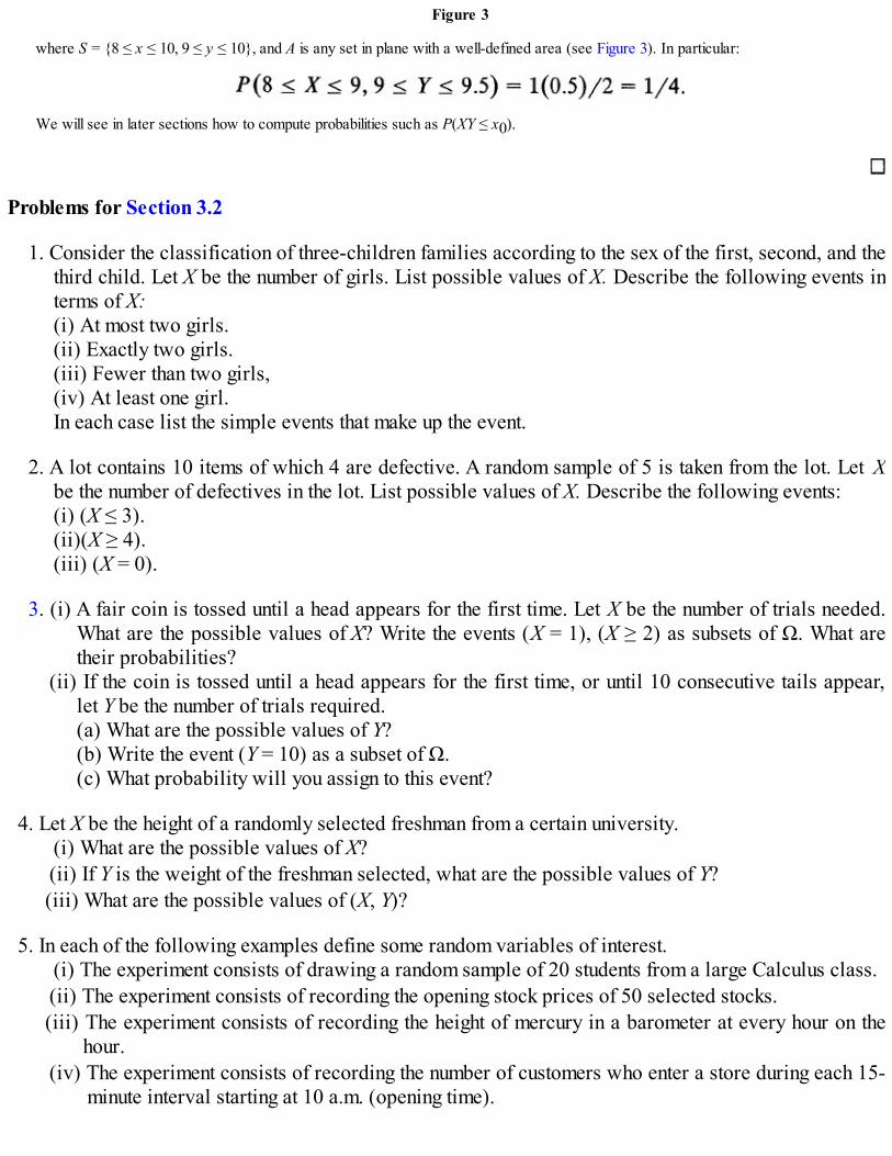
Figure 3

where S = {8 ≤ x ≤ 10, 9 ≤ y ≤ 10}, and A is any set in plane with a well-defined area (see Figure 3). In particular:

We will see in later sections how to compute probabilities such as P(XY ≤ x0).

Problems for Section 3.2

1. Consider the classification of three-children families according to the sex of the first, second, and thethird child. Let X be the number of girls. List possible values of X. Describe the following events interms of X:(i) At most two girls.(ii) Exactly two girls.(iii) Fewer than two girls,(iv) At least one girl.In each case list the simple events that make up the event.

2. A lot contains 10 items of which 4 are defective. A random sample of 5 is taken from the lot. Let Xbe the number of defectives in the lot. List possible values of X. Describe the following events:(i) (X ≤ 3).(ii)(X ≥ 4).(iii) (X = 0).

3. (i) A fair coin is tossed until a head appears for the first time. Let X be the number of trials needed.What are the possible values of X? Write the events (X = 1), (X ≥ 2) as subsets of Ω. What aretheir probabilities?

(ii) If the coin is tossed until a head appears for the first time, or until 10 consecutive tails appear,let Y be the number of trials required.(a) What are the possible values of Y?(b) Write the event (Y = 10) as a subset of Ω.(c) What probability will you assign to this event?

4. Let X be the height of a randomly selected freshman from a certain university.(i) What are the possible values of X?(ii) If Y is the weight of the freshman selected, what are the possible values of Y?(iii) What are the possible values of (X, Y)?

5. In each of the following examples define some random variables of interest.(i) The experiment consists of drawing a random sample of 20 students from a large Calculus class.(ii) The experiment consists of recording the opening stock prices of 50 selected stocks.(iii) The experiment consists of recording the height of mercury in a barometer at every hour on the

hour.(iv) The experiment consists of recording the number of customers who enter a store during each 15-

minute interval starting at 10 a.m. (opening time).

6. Consider families with four children. Define X by X = 1 if the first born was a girl and zerootherwise, and Y by Y = 1 if the fourth child was a girl and zero otherwise. Write down the events (X= 0, Y = 0), (X = 1, Y = 0), (X = 0, Y = 1), (X = 1, Y = 1) as events in the sample space (Ω, ζ). Whatprobabilities will you assign to these events if boys and girls are equally likely?

7. A committee of four is selected from a group of 10 students consisting of 4 seniors, 2 juniors, 2sophomores, and 2 freshman. Let X be the number of seniors and Y the number of juniors in thecommittee. Describe the events (X = 1, Y = 0), (X = 3, Y = 1), (X = 2, Y = 1), (X = 1, Y = 1). Whatprobabilities will you assign to these events?

8. Suppose Ω = [0,1]. Let ζ the set of events in Ω and suppose P on ζ is defined as follows. To eachsubinterval (a, b] of Ω, P assigns probability

Define X on Ω be setting X(ω) = 2ω + 1.(i) What are the possible values of X?

(ii) Find P(X ≤ 2), P(X > 1), P(a < X ≤ b).

9. Let Ω = [ – 2, 1] and ζ the set of events on Ω. On ζ let P be defined as follows: To each subintervalof (a, b] of Ω, P assigns probability

Let Y be defined as follows:

(i) What are the possible values of Y?(ii) Find P(– 3 < Y ≤ 1), P(Y ≤ 0), P(Y > – 1).

10. Let Ω = {(ω1, ω2): 0 < ω1 < ω2 < 1}. Suppose P on ζ is defined as follows: For A ⊆ Ω, A ∈ ζ, P(A) =

. Let

Find P(X < 1/2), P(Y > 1/2), P(1/3 < X < Y < 5/8).

3.3 DESCRIBING A RANDOM VARIABLE

We began with the following description of a random experiment. Identify Ω, the set of outcomes of theexperiment, ζ, the events of interest, and define probability P on ζ. Then the triple (Ω, ζ, P) gives astochastic description of the experiment. In Section 3.2 we saw how we transform Ω into a more

convenient set of outcomes whose elements are real numbers. We indicated how to identify events on thissample space and how to compute probabilities of these events. The mathematical description of themodel is complete once we know X, the events of interest, and the induced distribution Px of X. Thissituation is different from that in calculus. There we identify the domain set D and the recipe f whichassociates with each x ∈ D some real number f(x). Knowledge of D and f gives a complete description ofthe model. In statistics the description is not complete until one specifies in addition the distribution of X.

The specification of Px through P on (Ω, ζ) is not satisfactory since one frequently has to compute Pxfor an incredibly large set of events according to the formula

where A is an event on the new sample space, A ⊆ . Fortunately it is not necessary to do so. In thissection we study two equivalent ways to specify Px. For this purpose it is convenient to consider twoseparate cases according to whether X takes values in a countable subset of or values in an intervalon . In the former case if = { x1, x2,…}, it is sufficient to specify P(X = xj) = P{ω: X(ω) = xj} foreach j. In the latter case it suffices to specify some nonnegative function f on such that

for each event A ⊆ .

DEFINITION 1. A random variable X on (Ω, ζ) is said to be of the discrete type if it takes values in a countable set = {x1, x2,…}, thatis, if the set of all distinct X(ω), as ω varies over Ω, is at most countable. The distribution Px of X is specified by the numbers

and {Px{xj}} is known as the probability function of X. For any event A in , that is, any subset A of , we have

DEFINITION 2. A random variable X is said to be of the continuous type if it takes all values over some interval, that is, the set {X(ω), ω∈ Ω} is an interval on . The distribution of X is then specified by specifying some nonnegative integrable function f on such that

for every event A ⊆ . The function f is known as the density function of X.

In most cases X is either of the discrete type or the continuous type. But mixed types can and do occurin practice. In this case there is a countable set of points x1, x2,… and a nonnegative function f such that

for every event A. We will restrict our discussion almost exclusively to discrete and continuous cases andcontent ourselves with a few examples of the mixed type.

In the discrete case 1 ≥ Px{xj} ≥ 0 for all j and

In the continuous case f(x) ≥ 0 for all x ∈ and

Often we need the probability P(X ≤ x) that is cumulated up to and including a real number x. This isjust a function (of x) on and is given a special name.

DEFINITION 3. (DISTRIBUTION FUNCTION). The distribution function of a random variable X on Ω, denoted by F, is defined by therelation

The basic reason why the distribution function is important is that it specifies and is completely specified by the distribution of X. Indeed,given Px for all intervals I, we get F by choosing I = (– ∞, x]. Conversely, suppose F is given. Then for any x1, x2 ∈ , x1 < x2, we have

from additivity of P on (Ω, ζ). Hence

so that

In the special case when x2 = ∞, we get

The probability P(X > x1) is called a tail probability and is often used to compare distribution functions.(See also Remark 8, Section 3.7.)

Thus a description of the model is complete the moment we specify F. Later we will show that this isequivalent to specifying the probability or density function of X.

What are some properties of F? What does it look like? Here are some simple properties.

PROPOSITION 1. Let F be a distribution function. Then(i) 0 ≤ F(x) ≤ 1 for all x ∈ ,(ii) x1 < x2 F(x1) ≤ F(x2) SO that F is nondecreasing,(iii) F is right continuous, that is, limx → x0

+ F(x) = F(x0) for all x0 ∈ (iv) limx → ∞F(x) = 1 and limx → – ∞F(x) = 0.

Proof. Part (i) follows from definition of F and part (ii) from (4). Part (iii) is proved in Lemma 1 below,and part (iv) follows from (iii) by letting x → ± ∞.

LEMMA 1. For any distribution function f and any real number x0

and

Proof*. Since F is nondecreasing and 0 ≤ F ≤ 1, the existence of the limits follows at once from calculus.(Any bounded monotone sequence has a limit.) We need only show that the limits have values indicated in(6) and (7). We prove only (6). The proof of (7) is similar. The idea of the proof is that as x → , theinterval (x0, x] shrinks. If P is “continuous” then we should have P(x0, x] → 0 as x → .

Let x > x0. Then

so that

Let … > xn > xn – 1 > ··· > x0 such that xn → x0. We need only show that P(x0 < X ≤ xn) → 0. Choose xn =x0 + l/n and set pn = P(x0 < X ≤ x0 + 1/n). Let An = (x0 + 1/(n + 1) < X ≤ x0 + 1/n). Then An’s are disjointand

Moreover,

The series converges, since . Hence

so that limN → ∞PN = 0 as asserted.Next we show that there is a 1–1 correspondence between the distribution function of a random

variable X and its probability (or density) function. This is simple. In the discrete case

and in the continuous case

gives the distribution function for X. Conversely, suppose F is given. Then from Lemma 1

If X is of discrete type taking values = {x1, x2, …} then

gives the probability function of X. In the continuous case we use the fundamental theorem of calculus toconclude that

for all x where F is differentiable. (See also Remark 3.)In a more advanced course it is shown that every function F defined on and satisfying (i) to (iv) of

Proposition 1 is a distribution function of some random variable. Moreover, from remarks followingDefinition 3 we note that F is determined by, and determines uniquely, a distribution Px on the set ofevents in through the correspondence (4) or, equivalently, PX((– ∞, x]) = F(x).

The following result is now somewhat obvious.

PROPOSITION 2.( i ) Given a set of nonnegative real numbers pk such that , then {pk} is the

probability function of some discrete type random variable X.( i i ) Given a nonnegative real valued function f that is integrable on and satisfies

, then f is the density function of some random variable X.

Proof. All we need to do is to construct a distribution function F. This is easy. In the continuous case forexample set

then F satisfies all the four properties of Proposition 1.

Remark 1. We emphasize that the distribution of X is uniquely determined by specifying either thedistribution function or the density (or probability) function. In the following the phrase “X has

distribution given by” will be followed by either the distribution function or the density (or probability)function. When we ask the reader to find the distribution of X, it is sufficient to find either the density (orprobability) function or the distribution function of X.

Remark 2. We note that if Ω is a discrete set, that is, a countable set of points, then any randomvariable X defined on Ω is necessarily discrete. However, if Ω contains an interval on , a randomvariable on Ω may still be discrete. In the discrete case, P(X = xj) represents the probability that X takesthe value xj. If P(X = xj) > 0 for some xj we say that X (or the corresponding distribution function) has a,jump of size P(X = xj) at xj and call xj a jump point. If X takes values in {x1, x2,…} then its distributionfunction F given by (8), namely,

has jumps of size

at each xj, j = 1,2,…. Figure 1 represents the probability function and distribution function of a typicaldiscrete type random variable.

In analogy to mechanics, we can think of a total mass of one unit distributed over the real line suchthat the mass distribution consists of point masses at x1, x2,….

Remark 3. In the continuous case we can get the distribution function from the density function by therelation (9) and, conversely, the density function from F by the relation (12). We note that f is not uniqueand may be defined arbitrarily at values of x where F’(x) is not defined. Also, F is everywherecontinuous (in fact, absolutely continuous) and from (10) P(X = x) = 0 for all x ∈ . (From (10) F iscontinuous at x if and only if P(X = x) = 0.) Thus for any a, b ∈ , a < b

Figure 1

whenever X is of the continuous type. The fact that P(X = x) = 0 for each x ∈ does not mean that Xcannot take the value x. From a relative frequency viewpoint it simply means that if the associatedexperiment is repeated n times, the relative frequency of the event (X = x) will tend to zero as n → ∞. Infact f(x) does not represent the probability of any event. From the mean value theorem if f is continuous atx then we can interpret f(x) Δx P(X ∈ [x, x + Δx]) for small Δx and f(x) as the probability per unit oflength at x. Figure 2 illustrates a typical density and associated distribution function.

In analogy to mechanics we can think of a total mass of one unit continuously spread over the real linein such a way that the probability associated with any set of points is the mass of the set. Then f(x)represents the mass density at x. Geometrically we can therefore interpret P(A) = ∫Af(x)dx as the areabounded by the set A and the curve f. This interpretation frequently simplifies computations ofprobabilities.

Remark 4. Remark 3 exhibits the fact that P(A) = 0 A = Õ and P(B) = 1 B = Ω. Thus P(A) = 0does not mean that A cannot happen, only that A has probability zero. A relative frequency interpretationof this statement may be given as in Remark 3. If P(A) = 0 we say that A is possible but highlyimprobable.

Figure 2. Typical density and distribution functions.

Remark 5. We note that we can define, equivalently, a continuous type random variable to be onewhose distribution function F has the representation (9) for some nonnegative function f on . This meansthat F is absolutely continuous. We emphasize that F may be continuous without being absolutelycontinuous so that continuity of F is not sufficient for a random variable X to be of the continuous type.

Remark 6. When X is a discrete type random variable taking values on equally spaced points, sayintegers, we will prefer to draw a probability histogram of the probability function of X. This is done bydrawing rectangles centered at each x value with heights proportional to the probability at x so that thearea of a rectangle with center x and width 1 represents P(X = x). Then the total area of the rectangles—that is, the area under the histogram—is one, and in analogy with the continuous case (Remark 3), we canuse areas to represent probabilities of intervals (or events).

Remark 7. In practice no real-world experiment or measurement can possibly yield a continuous typerandom variable. The assumption that X is of continuous type is a simplifying assumption leading to anidealized description of the model. If X measures height of a tree in feet, X takes discrete integer values. If

X is measured to the nearest inch, it still takes discrete integer values but the corresponding rectangles inthe histogram get narrower and the histogram has a much smoother appearance than in the previous case(see Figure 3). If we shrink the length of the base by making units of measurement smaller and smaller, thehistogram will tend towards a smooth curve representing the (idealized) density of X.

Figure 3. Histogram of the same data in feet and in inches.

Example 1. Tossing a Fair Coin. Let X be the number of heads in one toss of a fair coin. Then the probability function of X is givenby

and the distribution function by

We note that F has jumps at x = 0 and at x = 1. Figure 4a gives the graph of F, and Figure 4b gives the probability histogram of X.

Example 2. Life-Testing. Consider an experiment that consists of life-testing a piece of equipment such as a battery or a light bulb ora transistor. Let us take the starting time of the test to be time zero and measure the length of life of the piece of equipment until it fails.Then we can take Ω = [0, ∞). Many random variables can be defined on Ω. Suppose X denotes the life length (failure time) of the piece.Then X maps Ω on to itself so that = Ω = [0, ∞) ⊆ . Some events of interest in Ω are

Figure 4a. Graph of F, Example 1.

Figure 4b. Probability histogram of X, Example 1.

Suppose X has density function

Then the distribution function of X is given by

Suppose we terminate testing at time t0. Let Y be the time to failure if the equipment piece fails prior to time t0, and let Y = t0 if itsurvives time t0. Then Y is a mixed type random variable with a jump at t0. The distribution function of Y is given by

Figures 5a and 5b give the distribution function and density function of X and Figure 6 shows the distribution function of Y.

Figure 5a. F(x) = 1 – e– x, x > 0 and zero elsewhere.

Figure 5b. f(x) = e– x, x > 0 and zero elsewhere.

Figure 6. Graph of FY(y).

Probability computations are somewhat easier if F is known. Thus

and

which depends only on t2 – t1.

Example 3. Round-Off Error. Suppose the account balance of customers of a bank at the monthly billing time is rounded off to the

nearest dollar. Let X be the round-off error. Then X equals the true balance minus the balance after round-off to the nearest dollar. Asimple discrete model that one can use is described by

One can, however, use a continuous approximation to simplify computation by assuming that X has density function

Thus:

and for most practical purposes we get nearly the same result.

Figure 7

Example 4. A Mixed Distribution. Consider the function (see Figure 7)

We note that 0 ≤ F ≤ 1, F is right continuous, nondecreasing, and satisfies F( – ∞) = 0, F(∞) = 1. Hence F is a distribution function. Notethat F(0–) = 0 and F(0+) = 1/2 so that F is not continuous at 0 and hence it is not the distribution function of a continuous type randomvariable. There is a jump of size

at x = 0, and F is continuous for x > 0. Thus F is the distribution function of a mixed type random variable X described by

and for 0 < x ≤ 1, X has density f given by f(x) = (d/dx)F(x) = 1/2, and zero elsewhere. We note that necessarily

Example 5. Waiting for the First Boy. Consider a couple who would like a boy. Suppose they have children until they have theirfirst boy. Let X be the number of children they have before the birth of the boy. Then X takes values in (0, 1, 2,…}. Assume that boysand girls are equally likely and that the sex at each birth is independent of that on any other birth. Then for x ≥ 0, x integral:

Figure 8. Histogram.

due to independence. Clearly

so that P(X = x) = (1/2)x + 1, x = 0, 1,… defines the probability function of X and the distribution function is given by F(x) = 0 for x < 0and for x ≥ 0

where [x] is the largest integer ≤ x. The graph of probability histogram and distribution function are given in Figures 8 and 9. Thus

and

In particular,

Figure 9. Distribution function.

Example 6. Volume of a Sphere. Consider a sphere of radius X, where X has distribution function

Let us find the probability that the volume of the sphere is larger than v0, say. We first note that F is continuous everywhere anddifferentiable except at x = 0 and x = 1. Hence for x ≠ 0 or 1 we get the density of X on differentiating F to be

At x = 0 and x = 1 we can define f arbitrarily. We choose f(0) = 0, f(1) = 0 so that

Now the volume V of a sphere of radius X is given by V = (4/3)πX3. Clearly V ≤ (4/3)π and for 0 ≤ v0 < (4/3)π

Remark 8. We emphasize that the distribution function F and the density function f are defined for allreal numbers x. The probability function of a discrete random variable taking only values x1, x2,… withpositive probability may also be defined for all x ∈ by writing P(X = x) = 0 if x ∈ (x1, x2,…}. This iswhat we will do at least in the beginning. Sometimes however, we will specify P(X = x) for only those xfor which P(X = x) > 0 to conserve space. In the continuous case, we will specify f for all x ∈ . This isdone to avoid mistakes, since in the continuous case f is usually given by a formula and there is a tendencyto substitute the expression for f in the integral without regard to where it is positive and where it is zero.

We conclude this section with the following definition.

DEFINITION 4. A random variable X is said to have a symmetric distribution about a point α if

If F is the distribution function of X, then F is symmetric about α if

In particular, if X is of the continuous type with density function f, then X is symmetric about α if andonly if

If α = 0, we say that f (or F or X) is symmetric. Examples of symmetric distributions are easy to come by.The density functions

and

are both symmetric about θ. The probability function

is symmetric about 1/2.

Problems for Section 3.3

1. Are the following functions probability functions?

(i) and zero elsewhere.

(ii) p(x) = x/21, x = 1, 2, 3, 4, 5, 6, and zero elsewhere.(iii) p(x) = x2/55, x = 1, 2, 3, 4, 5, and zero elsewhere.(iv) p(x) = (x2 – 2)/50, x = 1, 2, 3, 4, 5, and zero elsewhere.

2. For each of the following functions find the constant c so that p is a probability function.(i) p(x) = c(1/4)x, x = 1, 2,…, and zero elsewhere.

(ii) p(x) = c(1/3)x(2/3)15 – x, x = 0, 2,…, 15, and zero otherwise.(iii) p(x) = c2x, x = 1, 2,… ,11, and zero elsewhere.In each case write down the distribution function.

3. Consider an urn containing 5 red and 3 black marbles. A random sample of size 3 is selected(without replacement). Let X denote the number of black marbles drawn. Find the probabilityfunction of X. Find P(1 ≤ X ≤ 3).

4. Suppose X has probability function given by:

Find P(X < 0), P(X even), P{X = 0|X ≤ 0}, P{ X ≥ 2|X > 0}.

5. For what values of c are the following probability functions?

(i)

(ii) p(x) = (2x + 1)c, x = 0, 1,… ,6, and zero otherwise?(iii) p(x) = xc, x = 1, 2,…, N, and zero elsewhere?In each case find the distribution function and compute P(X < 3), P(2 < X < 5). Find the smallest xfor which P(X ≤ x) > 0.5. Find the largest x for which P(X ≤ x) < 0.5.

6. A lot of 10 items contains 2 defectives. Let X denote the number of defectives in a random sample ofsize 3 (without replacement). Find the probability function of X, its distribution function, and P(0 < X< 2), P(X > 1) and P(X < 2).

7. The number of arrivals at a supermarket in any period of length t hours has probability functionP(X(t) = k) = (8t)ke– 8t/k! , k = 0, 1,…, and zero otherwise. Find P(X(.25) ≥ 1), P(X(.25) < 2),P(X(.25) = 1).

8. Which of the following functions are density functions:(i) f(x) = x(2 – x), 0 < x < 2, and zero elsewhere.

(ii) f(x) = x(2x – 1), 0 < x < 2, and zero elsewhere.

(iii) f(x) = exp{–(x – θ)/λ}, x > θ, and zero elsewhere.

(iv) f(x) = (l/2)exp{ – |x|}, x ∈ .(v) f(x) = sin x, 0 < x < π/2, and 0 elsewhere.(vi) f(x) = 1 – |1 – x|, 0 ≤ x ≤ 2, and zero elsewhere.

(vii) f(x) = 0 for x < 0, = (x + 1)/9 for 0 ≤ x < 1, = 2(2x – 1)/9 for 1 ≤ x < 3/2, = 2(5 – 2x)/9 for 3/2 ≤x < 2, = 4/27 for 2 ≤ x < 5, and zero elsewhere.

(viii) f(x) = 1/[π(1 + x2)], x ∈ .

9. In Problem 8, compute the distribution functions for the densities in parts (iii) to (viii).

10. For what values of c are the following functions density functions?

(i) f(x) = cx(2 – x), 0 < x < 2, and zero elsewhere.(ii) f(x) = 0 if x ≤ – 1, = c(x + l)if – 1 < x ≤ 2, = 3c if 2 < x ≤ 5, and zero elsewhere.(iii) f(x) = cx4(1 – x), 0 ≤ x ≤ 1, and zero elsewhere.(iv) f(x) = c/(a2 + x2), |x| ≤ a, and zero elsewhere.(v) f(x) = c/x5, x ≥ 1000, and zero elsewhere.

11. Are the following functions distribution functions? If so, find the corresponding density or probabilityfunctions.

(i) F(x) = 0 for x ≤ 0, = x/2 for 0 ≤ x < 1, = 1/2 for 1 ≤ x < 2, = x/4 for 2 ≤ x < 4 and = 1 for x ≥ 4.

(ii) F(x) = 0 if x < – θ, = if |x| ≤ θ, and 1 for x > θ where θ > 0.

(iii) F(x) = 0 if x < 0, and = 1 – (1 + x)exp(– x) if x ≥ 0.(iv) F(x) = 0 if x < 1, = (x – 1)/8 if 1 ≤ x < 3, and 1 for x ≥ 3.(v) F(x) = 0 if x < 0, and = 1 – e– x2 if x ≥ 0.

12. For what values of c are the following functions distribution functions of continuous type randomvariables?

(i) F(x) = c[arctan x + π/2}, x ∈ (ii) F(x) = 0, if x < 1, = c(x – 1)3 if 1 < x ≤ 3, = 1 if x ≥ 3.(iii) F(x) = 0, if x < 0, = cx2 if 0 ≤ x < r, = 1 if x ≥ r.(iv) F(x) = c arccos [(r – x)/r] if 0 ≤ x ≤ 2r, = 0 if x < 0 and = 1 if x ≥ 2r.

13. The length X of a randomly selected call (in minutes) at an exchange is a random variable whosedensity can be approximated by

Find the probability that a call will last:(i) More than 10 minutes.

(ii) Between 15 and 25 minutes.(iii) Less than 12 minutes.

14. A leading manufacturer of color television sets offers a four-year warranty of free replacement if thepicture tube fails during the warranty period. It is estimated that the length of life of the picture tubesused by this manufacturer has density function f(t) = (1/10)e– t/10, t > 0, and zero elsewhere. Whatpercentage of sets will have picture tube failures during warranty period? During the first year?

15. Let X be the radius of the opening of a finely calibrated tube. Suppose X has density function

Find the probability that the cross-sectional area πX2 of the opening is greater than 14.25.

16. Consider the random variable X of Example 6,which has density function

Let S = 4πX2 be the surface area of the sphere (of radius X). Find P(S > s0).

17. Consider a street car line of length l. Passengers board the street car at a random point X in theinterval [0, l] and it is assumed that the probability that a passenger will board the street car in asmall neighborhood of x is proportional to x(l – x)3. That is, suppose X has density f(x) = cx(l – x)3, 0≤ x ≤ l, and zero elsewhere. Find c and P(X > l/2).

18. The yearly incomes are usually modeled by the distribution function

where α > 0 and x0 > 0. What proportion of incomes are in excess of x1? What proportion ofincomes are between x2 and x3(x2 < x3)?

19. Let X1, X2, X3 be random variables with distributions given by

respectively. An auxiliary experiment is performed that assigns equal probability to X1, X2, and X3,and an observation is taken (on X1, X2, or X3) depending on the result of the auxiliary experiment.(i) Find the probability that the observation is greater than 2.

(ii) If a value greater than 2 is observed, what is the probability that is it was on X1 On X2? On X

20. Suppose P(X ≥ x) is given for a random variable X (of the continuous type) for all x. How will youfind the corresponding density function? In particular find the density function in each of the followingcases:

(i) P(X ≥ x) = 1 if x ≤ 0, and P(X ≥ x) = 1 – for x > 0; λ > 0 is a constant.(ii) P(X ≥ x) = 1 if x < 0, and = (1 + x/λ)– λ, for x ≥ 0, λ > 0 is a constant.(iii) P(X ≥ x) = 1 if x ≤ 0, and = 3/(1 + x)2 – 2/(1 + x)3 if x > 0.(iv) P(X > x) = 1 if x ≤ x0, and = (x0/x)α if x > x0; x0 > 0 and α > 0 are constants.

21. Let f be a symmetric density. Let a > 0. Show that:(i) F(0) = 1/2, where F is the distribution function.

(ii) P(X ≥ a) = 1/2 – dx.

(iii) F(– a) + F(a) = 1.(iv) P(|X| > a) = 2 F(– a) = 2[1 – F(a)].(v) P(|X| ≤ a) = 2F(a) – 1.

3.4 MULTIVARIATE DISTRIBUTIONS

Consider a random vector (X1, X2…, Xk), k ≥ 2, defined on (Ω, ζ, P). How do we describe the model interms of the new sample space, namely, k (or a subset k) and the set of events on this new outcomespace? Our object now is to study some equivalent ways of describing the induced distribution of (X1, X2,…, Xk) on . The development follows closely the univariate case (Section 3.3). If Ω is a discrete set,then the new sample space is also discrete, and is the class of all sets. In this case it suffices to specifythe so-called joint probability function, as we shall see. In the case when k or a rectangle in k is thenew sample space, the fundamental objects of interest are rectangles. Let us take k = 2 for convenience.Let (X, Y) be a random vector defined on (Ω, ζ), and let 2 be the new space of outcomes. Then the eventsof interest are of the type I1 × I2 where I1, I2 are intervals on . Actually the set of events of interest in 2is much larger; it includes all sets in the plane that have a well defined area such as circles, ellipses,triangles, parallelograms, and so on. The induced distribution PX, Y of (X, Y) is defined just as in the one-dimensional case by the relation

for every event A. In particular if A = I1 × I2 where I1, I2 are intervals on , then

is the probability that the outcome (X, Y) falls in I1 × I2. To give a simpler description of PX, Y weproceed as in Section 3.3.

DEFINITION 1. (JOINT PROBABILITY FUNCTION). A random vector ( X, Y) is said to be of the discrete type if there exists acountable set ⊆ 2 such that P(( X, Y) ∈ ) = 1. The distribution Px, Y is specified by the numbers

where (xi, yj) ∈ , i, j = 1, 2,… and {PX,Y{(xi, yj}} is known as the joint probability function of (X, Y). For any subset A of we have

DEFINITION 2. (JOINT DENSITY FUNCTION). A random vector ( X, Y) is said to be of the continuous type with joint density functionf(x, y) if for every event A ⊆ 2 the joint distribution of (X, Y) is given by

In the discrete case, 1 ≥ P(X = xi, Y = yj) ≥ 0 for all (xi, yj) and

In the continuous case, f(x, y) ≥ 0 for all (x, y) ∈ 2 and

We will mostly deal with either the discrete case or the continuous case, although mixed cases doarise in practice where one variable is a discrete type and the other a continuous type. Often we need theprobability P(X ≤ x, Y ≤ y), which is a function of (x, y) ∈ 2.

DEFINITION 3. (JOINT DISTRIBUTION FUNCTION). The joint distribution function of (X, Y) is defined by the relation

for all (x, y) ∈ 2.

Just as in the univariate case F determines and is completely determined uniquely by PX, Y, similarly Fdetermines and is completely determined by the joint density or joint probability function. It is thereforesufficient to specify F or the joint density (or probability) function of (X, Y) to complete the description ofthe model.

The joint distribution function has properties similar to a univariate distribution function. These arestated below. A result similar to Proposition 3.3.2 holds, but we will skip the details.

PROPOSITION 1. Let F be the joint distribution function of (X, Y). Then(i) 0 ≤ F(x, y) ≤ 1 for all (x, y),

(ii) F is nondecreasing in each argument,(iii) F is right continuous in each argument,(iv) F(– ∞, y) = 0 = F(x, – ∞) and F(∞, ∞) = 1, and(v) for every x1 < x2, < y2 the inequality

holds.

Proof. We need only prove part (v), since proofs of parts (i) to (iv) are similar to the proof of Proposition 3.3.1. The inequality (5) simply says(see Figure 1) that P((X, Y) ∈ (x1, x2] × (y1, y2]) ≥ 0. Indeed,

as asserted.

The reader will recognize that in the multivariate case joint distribution functions have an additionalproperty, namely, (5). It turns out that the conditions of Proposition 1 are also sufficient for a function F tobe a joint distribution function. Often a function of two variables satisfies (i)-(iv) of Proposition 1 but not(v). In that case F cannot be a joint distribution function (Problem 7; see also Example 6). Proposition 1can be extended to more than two variable case.

Figure 1. {x1 < X ≤ x2, y1 < Y ≤ y2}.

In the discrete case

and in the continuous case

Similarly, if F is known we can obtain PX, Y{(xi, yj)} or f(x, y) from it. For example, if the joint densityexists then it can be obtained from the joint distribution function according to the formula

for all (x, y) where F has a mixed partial derivative.One can show (as noted above) that any function p(x, y) satisfying

is the joint probability function of some random vector (X, Y). Similarly, any function f satisfying

is the joint density function of some random vector (X, Y).For the bivariate case

represents the volume of the solid formed by the surface f and the set A in the (x, y) – plane (see Figure 2).

Example 1. Lot Inspection. Consider a large lot that has two types of defective items. Let us call these defects of type A and typeB. Suppose an item is drawn at random. Define (X, Y) as follows. Let

and

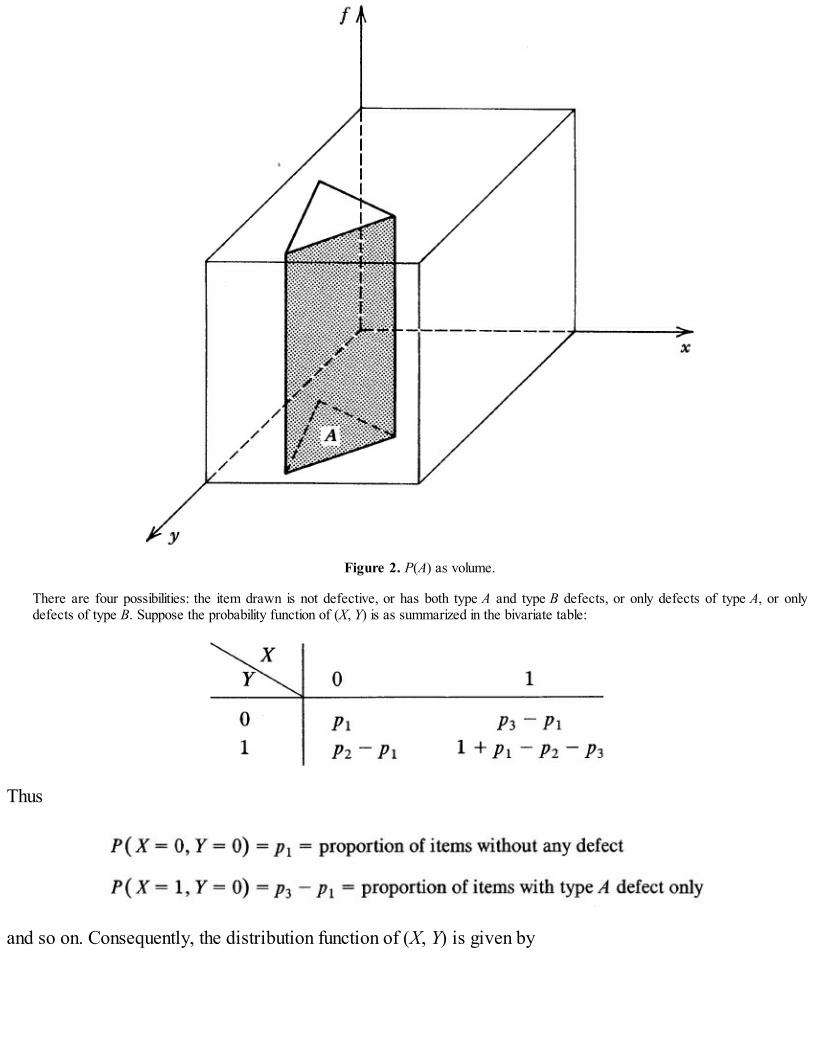
Figure 2. P(A) as volume.

There are four possibilities: the item drawn is not defective, or has both type A and type B defects, or only defects of type A, or onlydefects of type B. Suppose the probability function of (X, Y) is as summarized in the bivariate table:

Thus

and so on. Consequently, the distribution function of (X, Y) is given by

Figure 3 shows the joint probability function. Clearly

and

Example 2. Selecting a Committee. An ad hoc committee of three is selected randomly from a pool of 10 students consisting ofthree seniors, three juniors, two sophomores, and two freshmen students. Let X be the number of seniors and Y the number of juniors

selected. Let us compute the joint probability function of (X, Y). Clearly there are = 120 such committees and each is assigned the

same probability 1/120. Now

where n(i, j) is the number of ways of choosing i seniors (out of 3), j juniors (out of 3) and 3 – i – j sophomores of freshmen (out of 4) sothat from Rules 1 and 3 of Section 2.5

Figure 3

It follows that the joint probability function of (X, Y) is given by

It is easy to write the joint distribution function of (X, Y). Clearly,

and so on. Figure 4 shows the joint probability function of (X, Y).

Example 3. Tensile Strength. The tensile strengths X and Y of two kinds of nylon fibers have a joint density function proportional toxy exp{–(x + y)/λ}, x, y > 0.

Figure 4. Joint probability function of (X, Y).

Then the joint density function is given by:

Since f is a density function,

and it follows, on integration by parts, that c = 1/λ4. The joint distribution function of ( X, Y) is given by

and

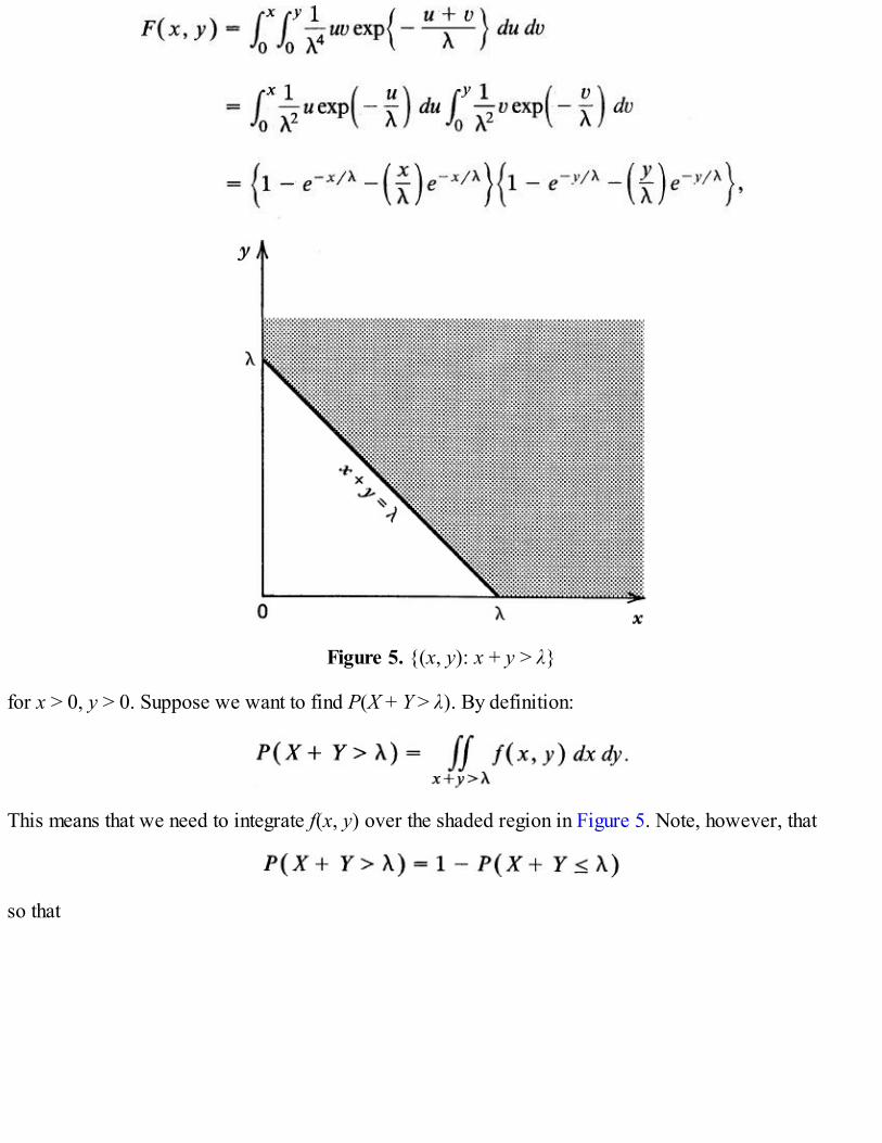
Figure 5. {(x, y): x + y > λ}

for x > 0, y > 0. Suppose we want to find P(X + Y > λ). By definition:

This means that we need to integrate f(x, y) over the shaded region in Figure 5. Note, however, that

so that

Example 4. Radar Screen. Let (X, Y) be the rectangular coordinates of a point on a circle of radius r and center (0, 0). For example,(X, Y) may be the coordinates of a spot on the circular screen of a radar station. Suppose (X, Y) has density function

Geometrically, f is just the circular section of a cylinder of height 1/(πr2) above the circle with center at the origin and radius r in the (x,y)-plane. The probability that (X, Y) ∈ A for any subset of the circle is proportional to the area of set A (see Figure 6). That is:

The probability that a spot will be observed in a square of diagonal 2 r, centered at the origin, is 2r2/πr2 = 2/π(Figure 7).We have from Figure 8 P(X > Y) = 1/2. Directly,

Figure 6. P{(X, Y) ∈ A}.

Figure 7

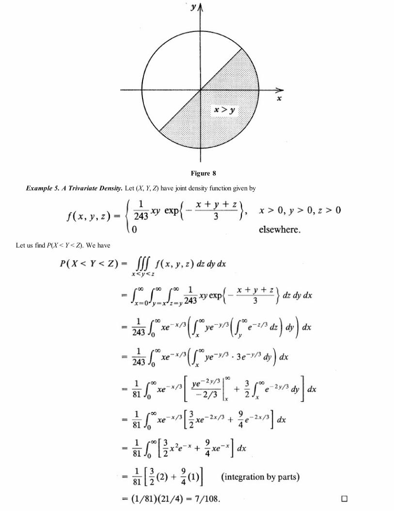
Figure 8

Example 5. A Trivariate Density. Let (X, Y, Z) have joint density function given by

Let us find P(X < Y < Z). We have

Example 6. Obtaining Density from a Joint Distribution Function. This example serves to illustrate two points: How do we showthat a function F is a distribution function? If so, how do we find the joint density in the continuous case? We will restrict ourselves to thecontinuous case. In view of the remarks following Proposition 1, we need to check conditions (i) through (v) in order to show that F is ajoint distribution function. Although (i) through (iv) are easily checked, (v) is not always easy to check. A quicker way, frequently, may beto use (7) to find f(x, y) and check to see if f is a density function. Consider the function

We note that 0 ≤ F(x, y) ≤ 1, F is nondecreasing and right continuous in each argument, and F(– ∞, y) = F(x, – ∞) = 0, F(∞, ∞) = 1. But(v) of Proposition 1 is not satisfied. Rather than find a rectangle for which (5) does not hold, we assume that F is a distribution function. Inthat case (7) gives the density function as

and since f < 0 for x, y > 0 we conclude that f cannot be a density function. Hence F is not a joint distribution function.Consider the function

Differentiating partially with respect to y and then with respect to x, we get

Since f ≥ 0 and (x, y) dy dx = 1, we see that f is a density function so that F must be a distribution function.

Problems for Section 3.4

1. A fair die is rolled twice. Let

(i) Find the joint probability function of (X, Y).(ii) Find P(X ≥ 8, Y ≤ 2), P(X ≤ 6, Y ≤ 3).

2. An um contains two black, one white, and three red marbles. A random sample of two marbles isdrawn (a) with replacement, and (b) without replacement. Let

for k = 1, 2. Find the joint probability function of (X1, X2) in each case, and also find the jointdistribution functions.

3. Four fair coins are rolled once. Let

(i) Find the joint distribution of (X, Y).(ii) Find P(X ≥ 3, Y ≥ 0), P(X ≥ 2, Y ≤ 1).

4. Consider the following joint probability function of (X, Y)

(i) Find P(X + Y ≥ 8), P(X + Y ≤ 7)(ii) Find P(6 ≤ XY ≤ 13), P(XY < 8).

5. An um contains five identical slips numbered 1 through 5. One slip is drawn and let X be the numberon the slip. Then all the slips numbered less than X are also removed from the um and another slip isdrawn from the remaining slips. Let Y be the number on the second slip drawn.(i) Find the joint probability function of (X, Y).

(ii) Find P(X ≤ 3, Y ≤ 4), P(X + Y ≤ 7), P(Y – X ≥ 2). (If X = 5, take Y = 0.)

6. Which of the following functions are joint density functions?(i) f(x, y) = e–(x + y), x > 0, y > 0, and zero elsewhere.

(ii) f(x, y) = xy, 0 ≤ x ≤ 2, 0 ≤ y ≤ 1, and zero elsewhere.(iii) f(x, y) = (1 + xy)/4, |x| ≤ 1, |y| ≤ 1, and zero elsewhere.(iv) f(x, y) = 8x2y, 0 ≤ y ≤ x ≤ 1, and zero elsewhere.(v) f(x, y) = (1 – e– x/λ1)(1 – e– y/λ2), x > 0, y > 0, and zero elsewhere.(vi) f(x, y) = x exp{ – x(1 + y)}, 0 < x < ∞, 0 < y < ∞, and zero otherwise.(vii) f(x, y) = e– y, 0 < x < y < ∞, and zero elsewhere.

7. Show that the following functions are not joint distribution functions.(i) F(x, y) = 0, x + 2y < 1, and 1 elsewhere.

(ii) F(x, y) = 1 – x exp(– x – y), x > 0, y > 0, and zero elsewhere.(iii) F(x, y) = 0, x + y ≤ 0, and 1 elsewhere.

(iv) F(x, y) = 1 – (1 – e– x)e– y, x > 0, y > 0, and zero elsewhere.(v) F(x, y) = 1 – exp{– x2 – y2}, x > 0, y > 0, and zero elsewhere.

8. Suppose (X, Y) is of the continuous type with joint density function f given below. Find c.(i) f(x, y) = c( 1 – x2 – y2), x2 + y2 ≤ 1, and zero elsewhere.

(ii) f(x, y) = cxe– y, 0 < x < y < ∞, and zero elsewhere.(iii) f(x, y) = c(x + y), 0 < x < 1, 0 < y < 1, 0 < x + y < 1, and zero elsewhere.(iv) f(x, y) = cxy, 0 < y < x < 1, and zero otherwise.(v) f(x, y) = c exp{–(x + y)}, 0 ≤ x ≤ y < ∞, and zero otherwise.(vi) f(x, y) = cg(x)g(y), – ∞ < x ≤ y < ∞, where g is a density function on (– ∞, ∞).In each case find the distribution function.

9. A point (X, Y) is selected at random from the unit circle according to joint density function f where fis proportional to the inverse of the distance of (X, Y) from the center of the circle. What is the jointdensity function of (X, Y)? Find P(1/2 < X < 1, 0 < Y < 3/4).

10. Let X be the lifetime of an electronic tube and Y that of the replacement installed after the failure of thefirst tube. Suppose (X, Y) have joint density f(x, y) = exp(– x – y), x, y > 0 and zero elsewhere. FindP(X + Y ≥ 2), P(X ≤ 5, Y ≤ 7), P(X/Y ≥ 1).

11. Is the function

a joint density function? If so, find P(X ≤ 7) where (X, Y, Z, U) is a random variable with density f.

12. Is the function

a joint density function? If so, find c. Also find

13. Consider an L.P. gas tank that has a random amount Y in supply at the beginning of the month. Supposea random amount X is used up during the month without being resupplied. Suppose X and Y have jointdensity function

where k is a known positive constant.

(i) Show that f is a density function(ii) Find the distribution function of (X, Y)(iii) Find P(X ≤ k/2), P(X ≤ k/2, Y ≥ 3k/4).

14. Consider an electronic system that has three types of components operating simultaneously. Thelifetimes X, Y, Z of the three components have joint distribution function given by

Find P(X > Y > Z). (See Problem 19 for a general result.)

15. Show that the function defined by

and zero elsewhere is a joint density function.(i) Find P(X > Y > Z > U).

(ii) Find P(X + Y + Z + U ≥ 1).

16. Let f1, f2,… fk be probability density functions on (a, b) where a may be – ∞ and b may equal ∞. Is

a density function of some random vector (X1, X2,…, Xk)? If so, find the distribution function of (X1,X2,…, Xk). Find P(X1 ≤ x, X2 ≤ x,…, Xk ≤ x) when f1 = f2 = … = fk.

17. Let A be a closed triangle in the plane with vertices (0,0), (0, ) and ( , ). Let F(x, y) denotethe area of the intersection of A with set {(x1, y1): x1 ≤ x, y1 ≤ y}. Show that F defines a distributionfunction. Find the corresponding joint density function. Find P(X + Y < 1), P(Y – X > 1).

18. Suppose (X, Y) are jointly distributed with density

where g is a density function on . Show that P(X ≥ Y) = P(X ≤ Y) = 1/2.

19. Suppose (X, Y, Z) are jointly distributed with density

Find P(X > Y > Z). Hence find the probability that (x, y, z) ∉ { X > Y > Z} or {X < Y < Z}. (Here g

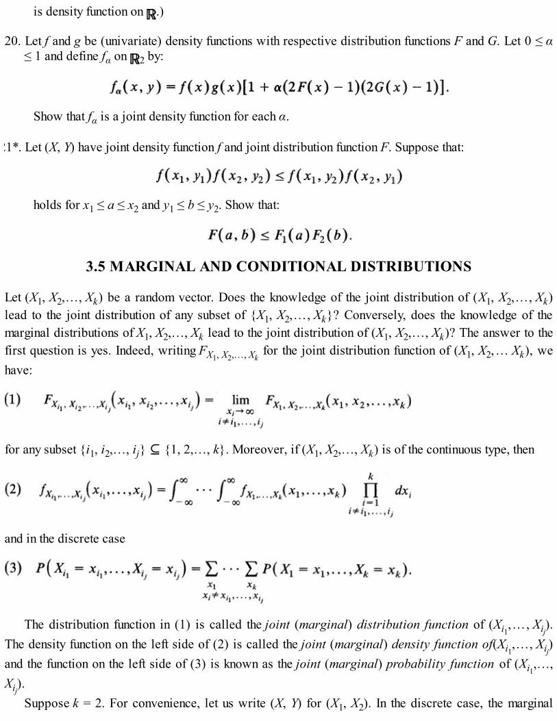
is density function on .)

20. Let f and g be (univariate) density functions with respective distribution functions F and G. Let 0 ≤ α≤ 1 and define fα on 2 by:

Show that fα is a joint density function for each α.

21*. Let (X, Y) have joint density function f and joint distribution function F. Suppose that:

holds for x1 ≤ a ≤ x2 and y1 ≤ b ≤ y2. Show that:

3.5 MARGINAL AND CONDITIONAL DISTRIBUTIONS

Let (X1, X2,…, Xk) be a random vector. Does the knowledge of the joint distribution of (X1, X2,…, Xk)lead to the joint distribution of any subset of {X1, X2,…, Xk}? Conversely, does the knowledge of themarginal distributions of X1, X2,…, Xk lead to the joint distribution of (X1, X2,…, Xk)? The answer to thefirst question is yes. Indeed, writing FX1, X2,…, Xk

for the joint distribution function of (X1, X2,… Xk), wehave:

for any subset {i1, i2,…, ij} ⊆ {1, 2,…, k}. Moreover, if (X1, X2,…, Xk) is of the continuous type, then

and in the discrete case

The distribution function in (1) is called the joint (marginal) distribution function of (Xi1,…, Xij).The density function on the left side of (2) is called the joint (marginal) density function of(Xi1,…, Xij)and the function on the left side of (3) is known as the joint (marginal) probability function of (Xi1,…,Xij).

Suppose k = 2. For convenience, let us write (X, Y) for (X1, X2). In the discrete case, the marginal

distributions of (X, Y) are easy to comprehend. In terms of a bivariate table, these are column and rowtotals that translate to the

graph in Figure 1. Basically it means that if we move a plane from left to right and another plane fromright to left, both parallel to the (x, P(X = xi, Y = yj))-plane until they meet the (x, P(X = xi, Y = yj))-plane,the marginal distribution of X is the total mass accumulated at various values of X in the (x, P(X = xi, Y =yj))-plane. A similar geometrical interpretation may be given to the marginal probability function of Y.

In the continuous case, the marginals of X and Y are the integrals of f(x, y) over all values of y and xrespectively. In geometric terms, the marginal density of X is the impression left on (x, f(x, y))-plane aswe condense the solid enclosed by f(x, y) by moving planes parallel to the (x, f(x, y))-plane from left toright and right to left until they meet the (x, f(x, y))-plane.

In what follows we restrict ourselves to the k = 2 case. For convenience we use the notation (X, Y)instead of (X1, X2). We now consider the second question raised in the first paragraph of this section.Does the knowledge of the marginal distributions of X and Y yield their joint distribution? The answer, ingeneral, is no. A special case where the answer is yes will be considered in Section 3.6. The fact that theanswer in general is no should not be surprising; the marginal distributions of X and Y provide noinformation on the dependence structure between X and Y. This information is provided by the conditionaldistribution defined below.

Figure 1. Marginal probability functions.

Suppose a value of X is observed. Given X = x, what is the distribution of a future value of Y? Thislooks like a problem in conditional probability. In the discrete case, given X = xi, the probability that Y =yj is given by

by the definition of conditional probability, provided that P(X = xi) > 0. Here X = xi is fixed and yj varies.We note that

and

by definition of the marginal probability function of X. Hence P{Y = yj|X = xi} , j = 1, 2,… defines aprobability function.

DEFINITION 1. Let (X, Y) be a discrete type random vector. Then the function defined by

for j = 1, 2,… is called the conditional probability function of Y given X = xi. We define P{Y = yj|X = xi} = 0 if P(X = xi) = 0.

Since P{Y = yj|X = xi} is a probability function it has all the properties of a probability function. Thus

In particular, if A = (– ∞, y], then

is called the conditional distribution function of Y given X = xi.In geometric terms, P{Y = yj|X = xi} is the cross section of P(X = xi, Y = yj) in the X = xi plane

adjusted to give a total mass of one. The adjustment factor is P(X = xi).

Example 1. Coin Tossing. Consider three independent tossings of a fair coin. Let

X = number of heads,

and

Y = number of tails before the first head.

Then X takes values 0, 1, 2, 3, and Y takes values 0, 1, 2, 3. The joint distribution of (X, Y) is given in the following table.

The row totals give the marginal distribution of Y and the column totals give the marginal distribution of X. Let us compute the conditionaldistribution of X given Y = y for y = 0, 1, 2, 3 respectively. We have

and

In particular,

and so on. The conditional distribution function of X given Y = 0, for example, is given by

In Figure 2, we plot the marginal distribution of Y and the conditional distribution of X, given Y = 0.

Example 2. Quality Control. Every manufacturer of major appliances such as washers, dryers, and refrigerators is concerned aboutthe quality of the merchandise before shipping. Suppose a manufacturing firm subjects its finished product to a final inspection thatconsists of looking for two kinds of defects, those in the finish (scratches, dents, and flaws in porcelain finish) and those that can beclassified as mechanical. A random sample of 100 pieces of the appliance is examined. Let X be the number of defects of the first kind,and Y the number of defects of the second kind.

Figure 2. Marginal distribution of Y (dotted line); conditional distribution of X given Y = 0 (solid line).

Suppose the following results are obtained.

In a situation such as this example, the joint distribution of (X, Y) will be estimated by the manufacturer after repeated sampling over aperiod of time. Suppose this table reflects the long-run joint distribution of defects. Then the probability function is obtained by dividingthrough by 100. The marginal distributions are then given by

and, in particular,

Thus

Similarly,

Let us now consider the case when X and Y have a joint density f. Let f1, f2 be the marginal densities ofX and Y respectively. Since P(X = x) = 0 for every x we can no longer follow the above development inorder to define the conditional distribution of Y given X = x. However, we can imitate (4) and set for f1(x)> 0

Then

and g(y|x) is a density function.

DEFINITION 2. Let (X, Y) be a continuous type random vector with joint density function f and let f1 be the marginal density of X.Then the conditional density of Y given X = x is defined by

provided f1(x) > 0.

We recall that a density may be changed on a finite set without affecting its integral, so that g(·|x) isnot strictly unique. When we speak of the conditional density, we simply mean that a version is chosenand held fixed. It is clear that the roles of X and Y may be reversed to define the conditional densityfunction of X given Y = y.

We now provide a justification for Definition 2. The reader may skip the following discussion. It isnot needed in our subsequent investigation.

Let h > 0 and suppose P(x – h < X ≤ x + h) > 0. By the definition of conditional probability, we have

Let F be the joint distribution function of (X, Y), f the joint density, and f1 the marginal density of X. Notethat since F1 (the distribution function of X) is continuous,

Moreover, (x – h < X ≤ x + h)↓(X = x) as h ↓ 0. Let us write

provided that the limit exists. Then

Both numerator and denominator tend to 0 as h ↓ 0 and we have a typical case of L’Hôpital’s rule.Dividing numerator and denominator on the right side of (12) by 2h and noting that if f1 is continuous at x,then

and

we have

provided f1(x) > 0.We note that P{Y ≤ y|X = x} defines a distribution function as a function of y for fixed x. This is called

the conditional distribution function of Y given X = x. Differentiating with respect to y we have

provided f is continuous at (x, y), f1 at x, and f1(x) > 0. This is precisely (9).Sometimes the notation fY|X(y|x) is used to denote the conditional density function and to denote the

conditional distribution function of Y given X = x. For convenience we will not use this subscript notationunless necessary. Whenever we write g(y|x) [or h(x|y)] it will mean the conditional density of Y given X =x (or of X given Y = y): the first letter within the parentheses is the variable, the letter following thevertical bar is fixed (and represents the given value of the random variable).

Geometrically, g(y|x) represents the cross section of f(x, y) in the X = x plane, adjusted so as to give atotal area of 1 under the curve.

Since g(y|x) is a density function, we can compute P{Y ∈ A|X = x) from the formula

It follows from the definition of conditional probability or density function that

and

where f2 is the marginal density of Y and h(x|y) the conditional density of X given Y = y.Relations (16) and (17) answer the second question we raised. In order to obtain the joint distribution

of (X, Y) we need one marginal and one conditional distribution (given the marginal). We note that forf2(y) > 0

which gives the continuous analog of the Bayes rule (Proposition 2.6.3).Often, one of X and Y is continuous type and the other discrete type. That is, (X, Y) is the mixed type. It

should be easy for the reader to modify the above discussion to include such a possibility. We willconsider some examples of this type here and later in Sections 10.6 and 10.7.

Remark 1. The reader should carefully distinguish between two types of problems involvingconditional probability. The problem of finding, say, P{X B | Y ∈ A} where P{Y ∈ A} > 0 is a simpleproblem of conditional probability to be treated by methods of Section 2.6. The problem of finding P{ X∈ B| Y = y}, however, is a problem of conditional probability distribution to be treated by methods of thissection. In the case when Y is discrete and P(Y = y) > 0, however, this distinction is not necessary.

Example 3. Target Practice . In target practice, a marksman aims a gun at a certain target, say, the origin of a rectangularcoordinate system, but due to random factors the hit-point can be any point (X, Y) in a circle of radius r with center at the origin. Suppose(X, Y) have joint density

(See also Example 3.4.4.) Let us compute f1, the marginal density of X. We have:

for |x| ≤ r, and zero elsewhere. By symmetry:

Consequently, for fixed x ∈ ( – r, r), Thus

Thus

Figure 3 shows the marginal distribution of X and the conditional distribution of Y given X = x.In the same target model, suppose the marksman has more skill so that the joint density function is more concentrated towards the

target, that is, the center of the circle. The joint density function

describes such a density function.The marginal densities are easily computed. Indeed,

for |r| ≤ x and zero elsewhere. The conditional density of Y given X = x for x ∈ (– r, r) is given by

Figure 3. Graphs of f1 and g.

Example 4. Sale Price and Volume of Sales. Suppose the selling price p of an article varies over the interval (0, 1) depending on thefinal production costs (determined from an initial run). The sales volume V is also a random variable depending on the selling price. Let thejoint density be given by:

Then

and zero elsewhere, and

and zero elsewhere. It is easy to compute f2 explicitly on integration by parts. We leave the details to the reader. It follows that for p ∈(0, 1),

Hence

In particular, if p = 1/2, then

Example 5. Additives in Gasoline. Let Xand Y be the proportions of two different additives in a sample taken from a certain brandof gasoline. Suppose the joint density of (X, Y) is given by:

By symmetry, X and Y have the same marginal densities, and the common density is obtained by integrating f over the shaded trianglein Figure 4b. Indeed, for 0 ≤ x ≤ 1

Figure 4a. Graph of g(y| ).

Figure 4b. {(x, y): f(x, y) > 0}.

and f1(x) = 0 elsewhere. The conditional density of Y given X = x is given by

for 0 ≤ x ≤ 1. In particular, if x = 1/3, then

and

Example 6. A Mixed Distribution: Store Holdups. The weekly number of store holdups in a certain city has probability function

We write Pλ instead of P to indicate that the distribution depends on λ. Once λ is specified we can compute probability of events definedin terms of X. Here λ > 0 measures the intensity of the incidence of holdups. Suppose the intensity varies from week to week according tothe density function

Let us call this random variable Λ. Then Pλ(X = x) gives the conditional distribution of X given Λ = λ, and the joint distribution of X and Λis given by

and zero elsewhere. The unconditional distribution of X is given by

for x = 0, 1, 2,… . Integrating by parts repeatedly, we get†Thus

where we have used the fact that (see Section 6.5), so that five or more holdups in aweek are highly improbable. If λ = .1 for a week, for example, then

whereas if λ = 10, then

The conditional probability Pλ(X ≥ 5) fluctuates between 0 and 1 depending on the value of λ. The unconditional probability P(X ≥ 5) is insome sense an average probability that takes into account the distribution of Λ. Since large values of Λ are improbable it is not surprisingthat P(X ≥ 5) is small.

Suppose we know that in some week X = 2. What can we say about Λ? The information about Λ, given X = x is provided by theconditional density g(λ|x). For x ≥ 0 (integral) we have

and

Thus

and

If X = 2 is observed then it is improbable that Λ is large, that is, Λ ≥ .5, and much more probable that Λ is small, .1 ≤ Λ ≤ .3.

We conclude this section with some remarks concerning the more than two variate case. Let (X1, X2,…, Xk), k ≥ 2, be a random vector defined on (Ω, ζ, P). We have seen in (1) through (3) how to obtain thejoint marginal distribution of a subset of X1, X2,…, Xk from the joint distribution of (X1, X2, …, Xk). Wecan also define the conditional distribution in a similar manner. Indeed, suppose (X1,…, Xk) is of discretetype, and we want to find the (joint) conditional distribution of (X1, X2,…, Xj) given Xj + 1, …, Xk, for j <k. Then:

provided P(Xj + 1 = xj + 1,…, Xk = xk), the marginal probability function of (Xj + 1,…, Xk), is positive at (xj

+ 1, …, xk). In the continuous case the conditional density of (X1, X2,…, Xj) given Xj + 1 = xj + 1,…, Xk = xkis defined by

for all (x1,…, xj) provided . Here f is the joint density of (X1,…, Xk) and

that of (Xj + 1,…, Xk). It suffices to consider an example.

Example 7. Choosing Points from a Line Segment. A point X1 is chosen from [0, 1] such that the probability that X1 belongs to asmall neighborhood of x is proportional to the length of the neighborhood. That is, X1 has density

for x in a neighborhood of length Δx. Since f1 has to be a density on [0, 1], c = 1 and

A point X2 is now chosen from [0, X1] according to the density

Another point X3 is chosen from the interval [0, x2] according to the density

and so on. Suppose X1, X2,…, Xn are n such points. Then the joint density of (X1, X2,…, Xn) is given by:

This follows from an obvious extension of the product rule (17). Hence

Let k < n. Then the joint marginal density of (X1,…, Xk) is given by

and the conditional density of (Xk + 1,…, Xn) given X1 = x1,…, Xk = xk is given by:

and zero elsewhere.

Problems for Section 3.5

1. Consider a fair die that is rolled three times. Let X be the number of times the face value is 1 or 2,and Y the number of times the face value is 4, 5, or 6.(i) Find the joint distribution of (X, Y).

(ii) Find the two marginal distributions.(iii) Find the conditional distribution of X given Y = y and that of Y given X = x.(iv) Find P(1 ≤ X ≤ 3|Y = 1).

2. A fruit basket contains five oranges, two apples, and four bananas. The fruit are dropped in a sack

and a random sample of 4 is taken (without replacement). Let X be the number of apples and Y bethe number of bananas in the sample.(i) Find the joint probability function of (X, Y)

(ii) Find the two marginal distributions.(iii) Find the conditional distribution of Y given X = x (where x = 0 or 1 or 2).(iv) Find P{Y ≤ y|X = 1} for y = 0, 1, 2, 3, 4.(v) Find P{1 < Y < 3|X = 0}.

3. From a table of random numbers, a number X is drawn from the integers 1, 2, 3, 4, 5, 6. Suppose X =x. Then a second number Y is drawn from the integers x, x + 1,… ,9.(i) Find the joint probability function of (X, Y).

(ii) Find the two marginal distributions.(iii) Find the conditional distribution of X given Y = y.(iv) Find P{3 < X ≤ 9|Y = 8}

4. Let (X, Y) have joint probability function given by

(i) Find the marginal distributions of X and Y.(ii) Find the conditional distribution of X given Y = y.(iii) Find P{X ≤ 2| Y = 1}.

5. From a group of three Republicans, four Democrats and two Independents, a committee of three isselected. Let X be the number of Republicans selected and Y, the number of Democrats.(i) Find the joint distribution of (X, Y).

(ii) Find the two marginal distributions.(iii) Find the two conditional distributions.

(iv)Find P(X = 3), P(Y = 3). If the committee consists of either three Republicans or threeDemocrats, do the Independents have reason to complain? If the committee consists only ofDemocrats and Republicans, do the Independents have reason to complain?

(v) Find P{Y = 3|X = 0}, P{X = 3|Y = 0}.

6. For the following joint density functions, compute (a) the marginal distributions of X and Y, (b) thetwo conditional distributions.

(i) f(x, y) = 2(2x + 3y)/5, 0 < x < 1, 0 < y < 1, and zero elsewhere.(ii) f(x, y) = (x + y)/3, 0 < x < 2, 0 < y < 1, and zero elsewhere.(iii) f(x, y) = 1/2, 0 < x < 2, 0 < y < x, and zero elsewhere.(iv) f(x, y) = 8xy, 0 < x < y < 1, and zero otherwise.(v) f(x, y) = x exp{– x(1 + y)}, x > 0, y > 0, and zero otherwise.(vi) f(x, y) = (π2/8)sin(π(x + y)/2), 0 < x < 1, 0 < x < 1, 0 < y < 1, and zero otherwise.

(vii) f(x, Y) = 1/y, 0 < x < y < 1, and zero elsewhere.

7. Let X be the proportion of households that will respond to a mail-order solicitation and let Y be theproportion of households that will respond to a solicitation on the phone. Suppose (X, Y) have jointprobability density function given by:

(i) Find the two marginal densities.(ii) Find P(X > .25), P(Y ≤ .75).(iii) Find the two conditional densities.(iv) Find P{X ≥ .75| Y ≤ .25}, P{X + Y ≤ .50|X ≥ .25}

8. The joint distribution of (X, Y), where

is modeled by joint density function

(i) Find the two marginal distributions.(ii) Find the two conditional distributions.(iii) Find P{Y > 5|X < 10}, P{X > 10|Y ≤ 2}.(iv) Note that X – Y is the service time of the customer. Find

9. A point X is chosen from the interval [0,1] according to the density function f1 (given below).Another point Y is chosen from the interval [X, 1] (so that X ≤ Y ≤ 1) according to the densityfunction g(y|x). Let

and for 0 ≤ x < 1

(i) Find the joint density of X and Y and the marginal density of Y.(ii) Find the conditional density of X given Y = y.(iii) Find P{1/4 ≤ X ≤ 1/2|Y = 3/8}.

10. The surface tension X and the acidity Y of a certain chemical compound are jointly distributed withdensity function

(i) Find the two marginal densities, and the two conditional densities.(ii) Find P{X ≤ .92|Y = 1}, P{1 ≤ X + Y ≤ 2|X = .1}.

11*. Customers arrive at a service counter (a theater ticket booth or a bank teller’s or a retail counter),stand on line for service, and depart after service. Suppose X(t), the number of arrivals in a timeinterval of length t, has probability function

where λ > 0 is a fixed constant. Let T be the time it takes to service a single customer and let N bethe number of additional customers who arrive during the service time T of a customer. Suppose Thas density function

(i) Find the joint distribution of T and N and the marginal distribution of N.(ii) Find the conditional distribution of T given N = n.(iii) Find P(N ≥ 2), P{T ≤ 2|N = 2}. [Hint: P{N = n|T = t} = P{X(t) = n} = e–λt(λt)n/n!.]

12*. A new drug is designed to reduce the effects of a certain disease. Suppose the proportion X of patientswho respond favorably to the new drug is a random variable that has density function

The number of patients Y who show improvement from a total of n patients administered the drughas probability function

(i) Find the marginal probability function of Y.(ii) Find the conditional density of X given Y = y.

(iii)

Find P{0 < X < .1|Y = n}.[Hint: for α, β > 0

integral. See Section 7.3.]

13. Let f given below be the joint density of (X1, X2,…, Xn).

(i) f(x1, x2,…, xn) = e– xn, 0 < x1 < x2 < ··· < xn < ∞, and zero elsewhere.

(ii) f(x1, x2,…, xn) = (1/n!)exp( – max xi), x1 > 0, …, xn > 0, and zero otherwise.In each case find

(iii) the joint marginal density of (X3, X4,…, Xn), and

(iv) the joint conditional density of (X1, X2) given X3 = x3,…,Xn = xn.In (i) also find

(v) P{X2 – X1 > a|X3 = x3,…, Xn = xn }, for a > 0 fixed.

14. For distribution functions F, F1, F2 show that

for all x, y ∈ if and only if F1, F2 are the marginal distribution functions of F.

15. Let f1, f2 be density functions with corresponding distribution functions F1 and F2. Let α be a constant,|α| ≤ 1. Define

(i) The two marginal densities.(ii) The two conditional densities.

3.6 INDEPENDENT RANDOM VARIABLES

A basic problem in probability is to determine the joint distribution of the random vector (X1, X2,…, Xk)given the marginal distributions of X1, X2,…, Xk. In Section 3.5 we showed that in general we cannot getthe joint distribution from the marginal distributions alone. We need additional information on thedependence structure of X1, X2, …, Xk. If this information is available in the form of conditionaldistributions, then we can get the joint distribution. Thus, in the discrete case

This follows by a simple extension of the product rule (3.5.16). An analog of (1) holds also for thecontinuous case. An important special case is the case of independence which we now study. In this casethe probability that Xj ∈ Aj is unaffected by the values of the remaining random variables.

DEFINITION 1. Let X1, X2,…, Xk be random variables defined on (Ω, ζ, P). Then X1, X2,…, Xk aresaid to be independent if for all events A1, A2,…, Ak (in )

Definition 1 says that all the events {ω: Xj(ω) ∈ Aj) are independent on ζ and is a natural extension ofthe definition of independence of events. Definition 1 can be simplified and written equivalently in termsof distribution or density (probability) functions.

DEFINITION 2. Let F be the joint distribution function of (X1,…, Xk) and let Fj be the marginaldistribution function of Xj, j = 1, 2,…, k. Then X1, X2,…, Xk are independent if

DEFINITION 3. If X1,…, Xk are discrete type random variables then X1,…, Xk are independent if

for all x1, x2,…, xk ∈ .If (X1,…, Xk) have a joint density function f with marginal densities fj, j = 1,… k then X1,…, Xk are

independent if

for all x1, x2,…, xk ∈ .Definition 3 is the easiest to use in practice. We leave the reader to show that Definitions 2 and 3 are

equivalent. Definition 1 is also equivalent to Definition 2. Indeed, according to Definition 1

which is the statement of Definition 2. Conversely, according to Definition 2:

so that either

(in the discrete case) or

(in the continuous case) for all x1,…, xk. Now we sum both sides of (3) or integrate both sides of (4), asthe case may be, over all x1,…, xk such that xj ∈ Aj, j = 1,…, k. This leads to Definition 1.

Example 1. Family Incomes. Let X and Y represent the family incomes above $I of workers in two different trades. Suppose (X, Y)have joint density

Then X and Y are independent. Ineed, by symmetry

so that

We note that f(x, y) can be written as a product of a function of x alone and a function of y alone and the domains of X and Yseparate.

Example 2. Distribution of Children by Sex. Consider families with three children. Let X be the number of boys in a randomlyselected family and Y the number of girls. Since X + Y = 3, X and Y cannot be independent. Indeed, the joint distribution of (X, Y) is given(assuming boys and girls are equally likely) by

Since

X and Y are not independent. We note that to prove independence of X, Y we need to check (3) [or (4)] for all pairs, but to disprove

independence we need only find one pair (x, y) for which (3) or (4) does not hold.On the other hand, if we define U, V, Z as follows:

and

then U, V, Z are independent. This follows since

for u, v, z ∈ {0, 1} and P(U = u, V = v, Z = z) = 0 otherwise.

Example 3. Checking Independence. Suppose X and Y have joint density given by

The form of f does not suggest that we can write it as a product of two functions f1 and f2 where f1 is a function of x alone and f2 that ofy alone. Formally, for |x| < 1

and f1(x) = 0 elsewhere. By symmetry:

Thus f(x, y) ≠ f1(x)f2(y) and X and Y are not independent. Note, however, that for 0 < x < 1, 0 < y < 1,

so that X2 and Y2 are independent.

Independence is a very strong condition. If X1, X2, …, Xk are independent, that is, if (2) holds, then therandom variables in any subset of {X1, X2, …, Xk} are also independent. (Contrast relation (2) with theindependence of events A1, A2, …, Ak where we had to insist that the product relation holds for allsubcollections of A1, A2, …, Ak.) But we cannot go backwards. Independence of X1 and X2, X2 and X3, andX1 and X3 does not imply that of X1, X2, X3.

PROPOSITION 1. Let X1, X2, …, Xk be independent. Then(i) {Xi1,…, Xij} ⊂ { X1,…, Xk} are also independent,

(ii) any functions f1(X1),…, fk(Xk) are also independent, and(iii) any functions f(X1,…, Xj), g(Xj + 1, …,Xk) of disjoint subsets are also independent.

Proof. (i) By independence of (X1,…, Xk)

in an obvious notation. Now let xi → ∞ for all i = 1,…, k, i ≠ i1 or i2, …,ij. Then by definitionof a joint marginal distribution function and properties of distribution functions in onedimension, we have

(ii)We take k = 2 for convenience. Now the event {f1(X1) ≤ x1, f2(X2) ≤ x2} can be rewritten as {X1 ∈A1, X2 ∈ A2} where A1 depends only on f1 and A2 only on f2. Since X1, X2 are independent,

since Xj ∈ Aj if and only if fj(Xj) ≤ xj, j = 1, 2.(iii) By (i), (X1,…,Xj) and (Xj + 1,…,Xk) are independent. Hence the result follows from (ii).

What does independence say about conditional distributions? If (X1, X2) are independent, theprobability that X1 ∈ A1 is the same regardless of what happens to X2 so that the conditional distributionof X1 given X2 = x2 should not depend on x2. This is true. Indeed, in the continuous case

The same argument holds in the discrete case as also in the case when k > 2.

Example 4. Pairwise Independence vs. Independence. Suppose (X, Y, Z) have joint probability function

where A = {(1, 0, 0), (0, 1, 0), (0, 0, 1), (1, 1, 1)}. Then

for x, y ∈ {0, 1} and zero elsewhere. It follows that X, Y, Z are pairwise independent. That is, X and Y are independent, Y and Z areindependent, and X and Z are independent. But (X, Y, Z) are not independent since, for example,

Example 5. Ohm’s Law. Consider an electrical circuit for which the Ohm’s law V = IR holds where V is the voltage, I the currentand R the resistance. Suppose I and R are independent random variables with respective density functions

and

Then the joint density of I and R is given by

Thus (see Figure 1):

Figure 1. {(i, r): ir ≤ 2}.

Example 6. Lifetimes of Television Picture Tubes. Let X be the lifetime of a television tube manufactured by a certain companyand let Y and Z be the lifetimes of successive replacement tubes installed after the failure of the first tube. Suppose X, Y, Z areindependent with common density function

What is P(X + Y + Z ≥ 3λ)?By independence of X, Y, and Z, their joint density is given by

Hence:

where

It follows that

Example 7. Jury Discrimination: Cassell vs. Texas. In Cassell vs. Texas [399 U.S. 282 (1950)], black plaintiff Cassell wasconvicted of murder and appealed the decision on the grounds of jury discrimination. His argument was based on the fact that blacks wereunderrepresented on the juries in Dallas County. Although blacks formed 15.8 percent of the population in Dallas County, in a sample of21 juries examined only 17 of the 252 jurors (that is, 6.7 percent) were black. Moreover, no jury ever had more than one black on it.

The State of Texas argued that blacks formed only 6.5 percent of poll-tax payers. The Supreme Courtaccepted this explanation of the difference between the 15.8 percent and the 6.7 percent figures. Itreversed the conviction, however, on the basis of nonstatistical aspects of the case. Three judges notedthat it was quite improbable that no more than one black would every appear on a jury. Any such limit, itobserved, would be unconstitutional.

There are at least two kinds of jury discrimination problems here. Suppose we accept the figure of 6.5percent advanced by the State of Texas and accepted by the Supreme Court. Then p = proportion of blacks= .065. Let us first consider the problem of underrepresentation. Assuming that p = .065, how likely is itto observe 17 or fewer blacks in a random sample of size 252? If X denotes the number of blacks in asample of size 252, then this probability is given by

The argument used here is as follows. The probability of exactly k blacks and hence (252 – k) nonblacksby independence of selections is (.065)k(.935)252 – k. Since there are ways of choosing k blacks and

(252 – k) non-blacks, and since each selection has the same chance, it follows that (5) holds. (See Section6.3 for more details.) A probability such as the one in (5) is not easy to evaluate exactly. In Chapter 9 weconsider an approximation for the sum on the right side of (5), which yields

It is hardly reasonable to claim underrepresentation.The second problem here is that of limitation. That is, discrimination by arranging never to have more

than one black to a jury. Let X1, X2, …, X21 be the number of blacks on the 21 juries. Then

Assuming that Xi’s are independent, we have

P(Each of 21 juries has at most one black)

which is considerably smaller than P(X ≤ 17). Thus, under the assumption that blacks selected for eachjury formed a random sample of size Ω from a population that is 6.5 precent black, there is only 1.5percent chance that of the 21 juries examined each will have at most one black on it. Whether this issufficient evidence to conclude that there was discrimination (due to limitation of blacks) in jury selectionis a subjective judgment depending on the margin of error that one is willing to allow.?

Although the Supreme Court accepted the 6.5 percent figure, it is interesting to compare the twofigures: 6.7 percent blacks on juries and 15.8 percent blacks in the population. How likely is it to obtain arandom sample of size 252 that has 6.7 percent blacks from a population that has 15.8 percent blacks?Using the approximation mentioned above, one can show that this probability is approximately .0001. Intechnical language to be explained in Section 4.4, this means that the two proportions (sample andpopulation) are significantly different at level .0001. The general methods of comparing sample andpopulation proportions are discussed in Sections 4.4, 6.3, and 9.7.

Problems for Section 3.6

1. Given the joint distribution

Are X and Y independent?

2. If (X, Y) have joint probability function given by

are they independent?

3. Let (X, Y, Z) have probability function defined by

(i) Are X, Y, Z independent?(ii) Are X, Y, Z pairwise independent?

4. Suppose X1, X2 are independent having the same probability function given by

Let X3 = X1X2. Show that X1, X2, X3 are not independent but are pairwise independent.

5. Let A and B be events of positive probability and let X and Y denote the indicator functions of A andB respectively. That is, X(ω) = IA(ω) = 1 if ω ∈ A and zero otherwise. Show that X and Y areindependent if and only if A and B are independent events.

6. Let X and Y be independent random variables with probability functions given by

Find P(X + Y ≤ N/2) and P(X + Y ≤ N).

7. A retail outlet has two stores. In each store the daily demand for a particular item has probabilityfunction

where N is known. If the demands X1, X2 are independent, find P(X1 ≥ X2), P(X1 – X2 ≥ 5), P(X1 +X2 ≥ N). [Hint: ]

8. A fair die is rolled twice. Let X be the sum of face values and Y the absolute value of the difference

in face values on the two rolls. Are X and Y independent?

9. The random vector (X, Y) has joint density function f given below. Are X and Y independent?

(i) and zero otherwise

(ii) f(x, y) = xy 0 ≤ x ≤ 2, 0 ≤ y ≤ 1, and zero elsewhere.(iii) f(x, y) = 4y(x – y)e–(x + y), 0 ≤ y ≤ x ≤ ∞, and zero elsewhere.(iv) f(x, y) = 24y(1 – x), 0 ≤ y ≤ x ≤ 1, and zero otherwise.(v) f(x, y) = (1/2u2v), 1 ≤ u ≤ ∞, 1/u ≤ v ≤ u, and zero elsewhere.(vi) f(x, y) = 6x2y, 0 ≤ x ≤ 1, 0 ≤ y ≤ 1, and zero otherwise.(vii) f(x, y) = 2exp{– (x + y)}, 0 ≤ y ≤ x ≤ ∞, and zero elsewhere.(viii) f(x, y) = 8xy, 0 ≤ y ≤ x ≤ 1, and zero otherwise.

10. Let X, Y, and Z be the three perpendicular components of the velocity of a molecule of gas in acontainer. Suppose X, Y, and Z are independent with common density function given by

Let E be the kinetic energy of a molecule of mass m. Then E = m (X2 + Y2 + Z2)/2. Find P(E ≤ t) for t> 0 and, in particular, P(E ≤ a/2).

11. Suppose two buses, A and B operate on a route. A person arrives at a certain bus stop on this route attime 0. Let X and Y be the arrival times of buses A and B respectively at this bus stop. Suppose X andY are independent and have density functions given respectively by

What is the probability that bus A will arrive before bus B?

12. A leading manufacturer of TV guarantees its picture tubes for four years. Suppose the time to failureof its picture tubes has density function

If the time to failure of the tubes are independent, what is the probability that of the four televisionsets that are sold by a retailer:(i) All the picture tubes will fail during the guarantee period.

(ii) Only two will fail during the guarantee period.

13. Consider a simple electrical circuit for which Ohm’s law V = IR holds where V is the voltage, I thecurrent, and R the resistance. Suppose I and V are independent random variables with densityfunctions, respectively,

and

Find P(R > r0) where r0 is a fixed positive number.

14. The length X of time (in days) after the end of a certain advertising campaign that an individual is ableto remember the name brand of the product being advertised has density function

Suppose five individuals who viewed the campaign are independently selected 15 days after thecampaign ended.(i) Find the probability that none will remember the name brand.

(ii) Find the probability that only one will remember the name brand.What can you say about the success of the advertising campaign?

15. Consider two batteries, one of Brand A and the other of Brand B. Brand A batteries have a length oflife with density function

whereas Brand B batteries have a length of life with density function given by

Brand A and Brand B batteries are put to a test. What is the probability that Brand B battery willoutlast Brand A? In particular, what is the probability if λ = η?

16. Let X and Y be independent random variables of the continuous type. Find P(X > Y) in terms of thedensities f and g of X and Y respectively. In particular, if f = g find P(X > Y). (Problem 15 is a specialcase.)

17. Let X be the length (inches) and Y the width (inches) of a rectangle where X and Y are independentrandom variables with respective density functions

and

What is the probability that(i) The perimeter of the rectangle will be at least 36 inches?

(ii) The area of the rectangle will be between 60 and 80 square inches?

18. (i) Let (X, Y) have joint density f. Show that X and Y are independent if and only if for some constant k> 0 and nonnegative functions f1 and f2

for all x, y ∈ .(ii) Let A = {fx(x) > 0}, B = { fY(y) > 0}, and fX, fY are marginal densities of X and Y respectively.

Show that if X and Y are independent then {f > 0} = A × B.

3.7 NUMERICAL CHARACTERISTICS OF A DISTRIBUTION—EXPECTEDVALUE

Averages are part of our day-to-day life. We hear of the Dow Jones industrial average, the averagerainfall in a city in a year, the average temperature in July, the average age of workers in a plant, theaverage faculty compensation, and so on. We think of height relative to an average. A person is tall for hisor her age if he or she is taller than the average height for the group and short if he or she is shorter thanthe average for that group. Most people are comfortable with the Dow Jones industrial average as ameasure of general movement in stock prices. The average gasoline mileages announced by theEnvironmental Protection Agency have become a standard basis of comparison in automobile advertising.

Our aim in this section is to consider some numerical characteristics of a population distribution. Themost common average used in statistics is the mean or expected value or mathematical expectation.

Let X be a random variable defined on (Ω, ζ, P) and let g be a real valued function defined on .Define g(X) by

In all cases considered in this text g( X) is a random variable.

DEFINITION 1. Suppose g(X) is a discrete type random variable. If , then we define the meanof g(X) or the expected value of g(X) by

If g(X) is of the continuous type and f is the density function of X, then we define

provided that .

According to Definition 1, g(X) exists provided |g(X)| < ∞. Some special cases of interest arisewhen we take g(x) = x, g(x) = x – c, g(x) = |x|α, and we give these special names.

Example 1. Average Face Value in Rolling a Die. Suppose a fair die is rolled once. What is the average face value observed?Clearly X has probability function

Since X takes only a finite number of values, X exists and equals

Example 2. Average Number of Telephone Calls. Let Xt be the number of telephone calls initiated in a time interval of length t andsuppose Xt has probability function

Then

Note that Xt takes only nonnegative integer values with positive probabilities so that

Example 3. Average Length of Life of a Light Bulb. A manufacturer of light bulbs of a certain wattage approximates that the timeto failure X of light bulbs has density function

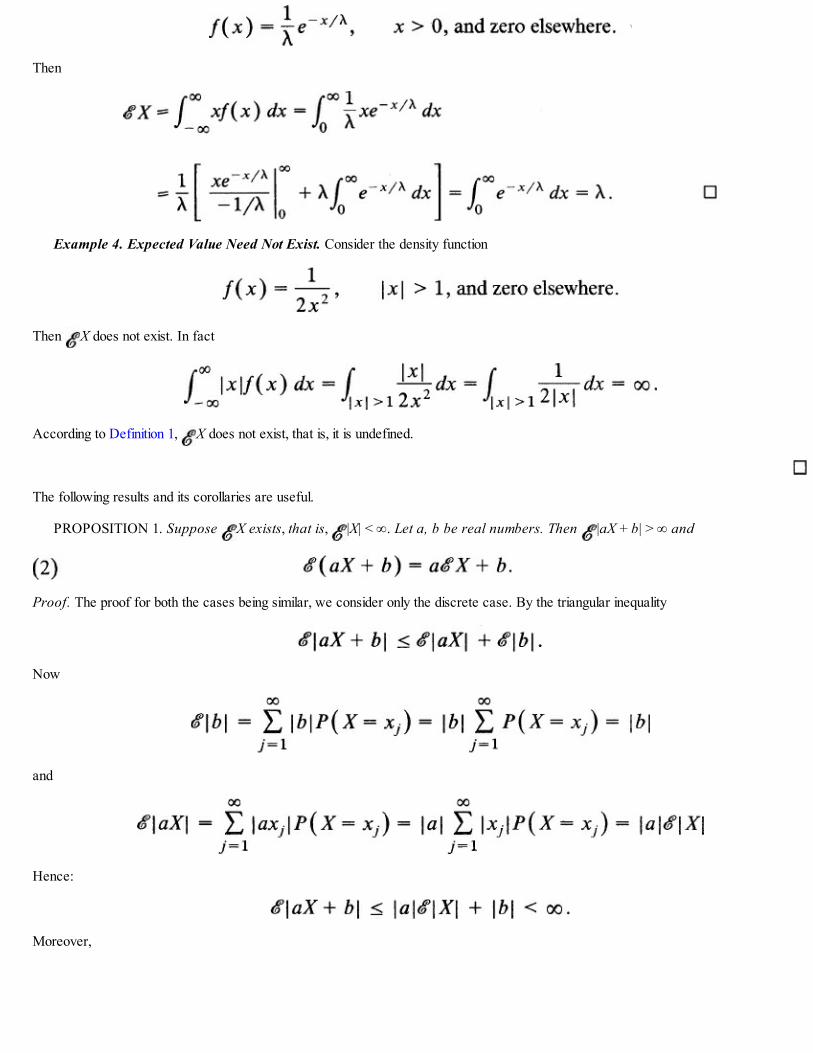
Then

Example 4. Expected Value Need Not Exist. Consider the density function

Then X does not exist. In fact

According to Definition 1, X does not exist, that is, it is undefined.

The following results and its corollaries are useful.

PROPOSITION 1. Suppose X exists, that is, |X| < ∞. Let a, b be real numbers. Then |aX + b| > ∞ and

Proof. The proof for both the cases being similar, we consider only the discrete case. By the triangular inequality

Now

and

Hence:

Moreover,

COROLLARY 1. If X exists then (X – X) = 0.Proof. Take a = 1 and b = – X in (2).

COROLLARY 2. Let g1, g2,…, gk be real valued functions such that g1(X),…, gk (X) are random variables. If |gj(X)| < ∞

for all j, then and

Proof. Use the triangular inequality to show the existence of and then split the left side of (3) into k separate sums

(or integrals) to get the right side of (3).

Remark 1. The term “expected value” is somewhat misleading in that X is not necessarily a value ofX to be expected when the experiment is performed. Thus in Example 1, the expected face value when afair die is rolled once is 3.5, which is not a possible value of X. From a relative frequency point of view,where we think of probabilities as limits of observable relative frequencies in repeated trials, theexpected value can be thought of as the limit of the averages (X1 + X2 + … + Xn)/n (as n → ∞) where X1,X2, …, Xn are the n observations on X when the experiment is repeated n times (see Section 3.8). Weshow in Section 5.4 that for large n the average (X1 + … + Xn)/n is likely to be near X. In Example 1this means that if the die is rolled n times then the average of the observed face values, for large n, islikely to be near 3.5.

Remark 2. The concept of expected value is analogous to the concept of center of gravity inmechanics. If we distribute a unit mass along the real line at points x1, x2, …, and if P(X = xi) is the massa t xi, then X represents the center of gravity. The same analogy holds in the continuous case. Ingeometric terms, this means that (in the continuous case) if we were to draw the density function f of X ona cardboard of uniform density, cut it along the curve, and balance it on an edge perpendicular to the x-axis at the point x = X, it will be in an equilibrium state (see Figure 1).

Many applications of probability involve minimization of expected loss or maximization of expectedprofit. We consider an example.

Example 5. An Inventory Problem. Stores order seasonal merchandise well in advance. Any article not sold is heavily discounted orremaindered at the end of the season. Suppose a store orders summer suits at a cost of $50 a suit which it sells at $150 per suit. At theend of the season, suppose the unsold suits are sold to a discount outlet at $35 per suit. From past experience it is known that theprobability function of the number of suits the store can sell to its customers is given by

How many suits must be ordered to maximize the expected profit?Let z be the number of suits ordered and stocked. Let φ(z) be the profit when z suits are stocked. Then

Figure 1

We note that φ(z) is a random variable which is a function of X. In view of the definition of g(X) we have

To find the value of z for which φ(z) is maximum we compute φ(z + 1) – φ(z). As long as φ(z + 1) – φ(z) > 0, φ(z) isincreasing as a function of z and the value of z at which φ(z + 1) – φ(z) changes sign gives us the maximum. We have

so that

It follows that

Thus the expected profit is maximum for the smallest value of z for which φ(z + 1) – φ(z) = 0 or negative. This value clearly dependson λ and can be computed once λ is specified.

Suppose λ = 5. In this case we want to find the smallest z for which either

Table A4 in the Appendix gives for various values of λ and z. For λ = 5 we see that

so that we must choose z = 8. The following table gives the values of z for some selected values of λ.

For large λ one can use normal approximation (Section 9.4). The probability function of X used here is the well known Poisson distribution,studied in detail in Section 6.5. The argument used to find the maximum of φ(z) is typical of discrete random variables and will be usedoften.

Remark 3. In this book we will use the terms “the mean of X” and “the mean of F “ interchangeablywhere F is the distribution of X.

3.7.1 Variance of a Random Variable

The center of gravity of a mass distribution provides no information about how the mass is spread aboutthis center. In mechanics, a measure of this spread (dispersion) is provided by the moment of inertia. Inprobability, X provides information only about the center or location of the distribution but says nothingabout how the distribution of X is spread about X. Indeed, it is possible to have many widely differentdistributions with the same mean or expected value. We now study a measure of variation, or dispersion,or spread that is analogous to the moment of inertia.

What we want is a measure that should take into account the deviations X – μ where μ = X. Since (X – μ) = 0 it is clear that we cannot use (X – μ) as a measure of spread. This suggests using |X – μ| asa measure of average dispersion. Unfortunately, the mean absolute deviation |X – μ| is not

mathematically tractable; manipulation with absolute values is not always easy. Yet another alternative isto consider |X – μ|2

DEFINITION 2. (VARIANCE). The variance of X (or of the distribution of X) is defined by

provided |X|2 < ∞, and is denoted by σ2. The (positive) square root σ is called the standard deviation of X.

It is usually convenient to compute the variance from the relation

Indeed, in view of Corollary 2 to Proposition 1

Remark 4. The following interpretation maybe given to the variance. Suppose you are asked to predicta value of X. If you predict the value to be c and X is observed, suppose you lose (X – c)2. Then your bestpredictor is c = X in the sense that it minimizes your average loss. Indeed, the average loss given by

is minimized for (c — μ)2 = 0, that is, for c = μ. Thus, if a fair die is tossed once, your best guess of theface value that will turn up is 3.5 even though you know in advance that a face value of 3.5 is impossible.(See Remark 1.)

The following proposition is very useful.

PROPOSITION 2. Suppose |X|2 < ∞.(i) We have

for some constant c.

(ii) For any real numbers a and b, we have

Proof. (i) Suppose there is a c for which P(X = c) = 1. Then X = c and Conversely, suppose var(X) = 0.Then P(X = μ) = 1. Indeed, in the discrete case suppose P(X = x) > 0 for some x ≠ μ. Then

This contradiction shows that there cannot be an x ≠= μ, for which P(X = x)> 0. Hence P(X = μ) = 1. Asimilar proof may be given in the continuous case.

(ii) First we note that |X|2 < ∞ implies, by triangular inequality, that |aX + b|2 < ∞ so that var(aX +b)exists. Now

COROLLARY 1. If X2 < ∞, and Z = (X – μ)/σ, then Z = 0 and var(Z) = 1.Proof. We have

and from Proposition 2(b)

Remark 5. The random variable Z defined in Corollary 1 is called the standardized X. Given arandom variable X we standardize it by subtracting from it the mean and dividing this deviation by thestandard deviation. This changes the origin to μ and the scale to standard deviation units. Standardizationis useful in comparing two or more distributions. Suppose for example that a student scores 80 on a

calculus test where the mean was 70 and the standard deviation 4, and she scores 75 on a statistics testwhere the mean was 60 and the standard deviation 5. At first glance it appears that the student did betteron her calculus test since her score was 80. Converting to standard units we note that her standard scoreon the calculus test was (80–70)/4 = 2.5 whereas here standard score on the statistics test was (75–60)/5= 3, so that her relative position in statistics class is better.

Remark 6. We note that var(X) > 0 for all nontrivial random variables. Moreover, if the distributionof X is concentrated near X then σ2 will be small. On the other hand, if values of X are widely dispersedthan σ2 will be large. We will see (Remark 9) that a small value of σ2 means the probability is small thatX will deviate much from its mean. But a large value of σ2 does not necessarily mean the probability islarge that X will be far from X (Problem 21).

Remark 7. We defined Xk as the moment of order k and (X – μ)k as the moment of order k aboutthe mean (also called the kth central moment of X). We note that if |X|n < ∞ for some n, then |X|k < ∞for k < n. Indeed, in the discrete case for k < n

Remark 8. Probabilities of the type P(|X| > n) or P(X > n) or P(X < – n) are called tail probabilities.The behavior of the tail probability determines whether |X|k < ∞ or not. In fact, if |X|n < ∞ then

and a partial converse also holds. We have:

so that as n → ∞. Since

we see that nkP(|X| > n) → 0 as n → ∞. In the converse direction, nkP(|X| > n) → 0 as n → ∞ implies that|X|k – δ < ∞ for all 0 < δ < k, but we will skip the proof.

Example 6. Variance Computation. Let X have density function

Then

and

Suppose Y has density

Then

and

It follows that

Figure 2 shows the graphs of f and g. The density g assigns more probability near the mean π/2 than the density f. It is not surprising thenthat var(X) > var(Y).

Example 7. Computing Variance and Higher Order Moments. Suppose X has density function

Clearly, Xk exists for any k and

Figure 2

Hence:

3.7.2 Chebyshev’s Inequality†

We now obtain a very useful inequality that gives an operational meaning to the definition of variance. Letus introduce the distance |X – X|. Let ε > 0. What is the chance that |X – X| ≥ ε?

THEOREM 1. Suppose X2 < ∞ and X = μ, var(X) = σ2, 0 < σ2 < ∞. Then for every ε > 0:

Proof. We give the proof only in the continuous case. We have

Since ε > 0, it follows that (7) holds.

COROLLARY 1. (CHEBYSHEV’S INEQUALITY). For any k ≥ 1,

or, equivalently,

Proof. Take ε = kσ in (7).

Remark 9. From (7) we see that the smaller the a, the smaller the probability P(|X – X ≥ ε). That is,if σ is small then the probability that X will deviate from μ by more than e is small. From (8), the largerthe k, the smaller the P(|X – μ| ≥ kσ). Thus

and

If σ is large however, it does not follow that P(|X – X| ≥ ε) will be large. (See Problem 21.)

Remark 10. The result (7) or (8) applies to all distributions for which |X2| < ∞. It is not surprising,therefore, that it provides a fairly crude bound for tail probabilities. We hasten to add, though, that theinequality is sharp. That is, it cannot be improved unless X is further restricted. Nevertheless, we willfind the inequality to be very useful and use it often.

Remark 11. Chebyshev’s inequality, in fact, is a property of any finite set of real numbers. In Problem28 we ask the reader to imitate the proof of Theorem 1 to show that if x1, x2,…, xn is any finite set of realnumbers, and

then at least a fraction (1 – 1/k2) of the n numbers are included in the interval .

Example 8. Choosing a Point on (0,1). A point is chosen from the interval (0,1) according to the density

Then X = 1/2, var(X) = 1/12, and according to Chebyshev’s inequality

For k = 2, , and for k = 3, P(X ≥ 1/2 + 3/ or X ≤ 1/2 –3/ ) ≤ .11. However, by direct integration

Figure 3

since 2/ .58 so that the Chebyshev’s inequality considerably overestimates the probability in the tail. In Figure 3 we compare theexact probability P(X – 1/2| ≥ kσ) with Chebyshev’s bound. Note that

Example 9. Chebyshev’s Inequality Is Sharp. Let X have probability function

and

Then

and

so that equality holds in (8).

Example 10. Some Typical Applications of Chebyshev’s Inequality. According to (9),

This inequality has three parameters μ, σ, and k . Given μ, σ, and k , it says that X ∈ (μ – kσ, μ + kσ) with probability at least 1 – 1/k2. Inpractice μ or σ are hardly if ever known. The object, then, is to find bounds for μ or σ that will cover the unknown μ or σ with a givenprobability, say 1 – α, 0 < α < 1.

Suppose μ is unknown but σ is known and we want to find a(X) and b(X) so that P(a(X) < μ < b(X)) ≥ 1 – α.We choose 1 – α = 1 – 1/k2 so that k = . Then

or, equivalently,

Thus a(X) = X – σα– 1/2 and b(X) = X + σα– 1/2. Similarly, if μ, is known, one can show that

Remark 12. Sometimes we will use (8) with strict inequality and (9) with < replaced by ≤ . It is clearthat (8) holds with “ ≥ kσ ” replaced by “> kσ” and (9) holds with “< kσ” replaced by “≤ kσ.”

3.7.3 Some Additional Measures of Location and Dispersion

We have seen that moments such as X and var(X) do not always exist. In such cases the theorydeveloped in the earlier sections is inapplicable. We now define some measures of location anddispersion which always exist.

DEFINITION 3. (QUANTILE OF ORDER p). Let 0 < p < 1. A quantile of order p of a randomvariable X (or the distribution Px) is any number ζp such that

or, equivalently,

For p = 1/2 we call ζ.5 a median of X.

If X has distribution function F, then ζp is a quantile of order p if it satisfies

In particular, if F is continuous at ζp then ζp is a solution of F(ζp) = p. However, it may still not be uniqueunless F is monotone. Graphically, Figure 4 illustrates computation of ζp. If the graph of F is flat at p thenζp is not unique. A median is frequently used as a center of the distribution and the difference ζ.75 – ζ.25,called the interquartile range, is used as a measure of spread or dispersion. Here ζ.25 is called the firstquartile and ζ.75 the third quartile of X. We note that X (if it exists) is influenced by extremely high orlow outcomes. In such cases a median may be preferable as a measure of location. Such is the case, forexample, when X is family income or annual wages.

Figure 4

Yet another measure of location is mode. A mode of a random variable (or a distribution) is its mostprobable value. In the case when X is of the discrete type, a mode of X is that value of X at which theprobability function P(X = x) has its largest value. If, on the other hand, X is of the continuous type, thenP(X = x) = 0 for all x. In this case a mode is that value of X for which f(x) is maximum. A mode may ormay not exist.

A distribution is said to be unimodal if the probability or density function has a unique maxima(Figure 5a) and bimodal if the probability or density function has two modes (Figure 5b). Most of thedistributions studied in this text are unimodal.

Example 11. Number of Arrivals at a Bank. Suppose the number of arrivals X at a bank in any 15-minute interval has probabilityfunction

Figure 5

This is the so-called Poisson probability function encountered in Example 5, for which the distribution function is given in Table A4 in theAppendix. The table below abridged from Table A4 gives P(X ≤ x).

From the definition of median, we see that since

ζ.5 = 5 is the unique median of X. Similarly,

so the interquartile range is 6 – 3 = 3. The modal value is 5 and the distribution is unimodal. We note that X = 5 so that X = ζ.5 =Mode (X).

Example 12. Survival Times of Patients with Advanced Cancer of the Bladder.Suppose the survival times of patients who have advanced cancer of the bladder can be modeled by the density function

Then X = λ so that the average time a patient survives is λ. We note that

for x ≥ 0. Since F is continuous, given 0 < p < 1, ζp is given by

It follows that

so that ζ.5 = λ ln 2, ζ.25 = λ ln(4/3), ζ.75 = λ ln 4. Thus about 50 percent of the patients will die by time λ ln 2, and about 25 percent willdie by the time λ ln(4/3). Since f is a decreasing function of x it follows that the mode is at x = 0.

Applications of median will appear quite often in this text.

Problems for Section 3.7

1. A used-car salesman sells 0,1, 2, 3, 4, 5, or 6 cars each week with equal probability. Find theaverage number of cars sold by the salesman each week. If the commission on each car sold is $150,find the average weekly commission.

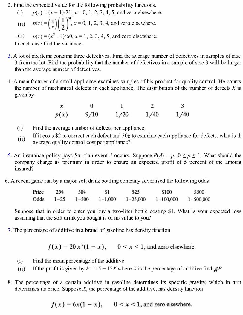
2. Find the expected value for the following probability functions.(i) p(x) = (x + 1)/21, x = 0, 1, 2, 3, 4, 5, and zero elsewhere.

(ii) p(x) = , x = 0, 1, 2, 3, 4, and zero elsewhere.

(iii) p(x) = (x2 + l)/60, x = 1, 2, 3, 4, 5, and zero elsewhere.In each case find the variance.

3. A lot of six items contains three defectives. Find the average number of defectives in samples of size3 from the lot. Find the probability that the number of defectives in a sample of size 3 will be largerthan the average number of defectives.

4. A manufacturer of a small appliance examines samples of his product for quality control. He countsthe number of mechanical defects in each appliance. The distribution of the number of defects X isgiven by

(i) Find the average number of defects per appliance.

(ii) If it costs $2 to correct each defect and 50 to examine each appliance for defects, what is theaverage quality control cost per appliance?

5. An insurance policy pays $a if an event A occurs. Suppose P(A) = p, 0 ≤ p ≤ 1. What should thecompany charge as premium in order to ensure an expected profit of 5 percent of the amountinsured?

6. A recent game run by a major soft drink bottling company advertised the following odds:

Suppose that in order to enter you buy a two-liter bottle costing $1. What is your expected lossassuming that the soft drink you bought is of no value to you?

7. The percentage of additive in a brand of gasoline has density function

(i) Find the mean percentage of the additive.(ii) If the profit is given by P = 15 + 15X where X is the percentage of additive find P.

8. The percentage of a certain additive in gasoline determines its specific gravity, which in turndetermines its price. Suppose X, the percentage of the additive, has density function

If X < .75, the gasoline sells as low test for $1.50 per gallon, and if X > .80, the gasoline sells ashigh test for $1.90 per gallon. Otherwise, it sells as regular for $1.75 per gallon. Find the expectedrevenue per gallon of gasoline sold.

9*. The newspaper boys or girls in a large city pay 18 for a newspaper that they sell for 25 . Unsoldnewspapers, however, can only be returned for 9 each. A newspaper girl has observed that her dailydemand has approximately the probability function given by

How many papers must she stock to maximize her expected profit?

10. A manufacturer of heat pumps offers a five-year warranty of free repair or replacement if thecondenser fails. The time to failure of the condenser it uses has density function

(i) Find the average time to failure of a condenser.(ii) Find the probability that a condenser will fail before the mean time to failure.

(iii) If the profit per sale is $550 and the replacement or repair cost of a condenser is $200, find theexpected profit.

11. The acidity of a compound X depends on the proportion Y of a certain chemical present in thecompound. Suppose

where α, β are constants. If the density of Y can be assumed to be

find the average acidity of the compound. Also find var(X).

12. It costs a company $C1 in fixed costs (irrespective of the volume of its production) and a variablemanufacturing cost of $C2 per piece of equipment it produces. All the pieces it produces are sold at$C3 each. The density function of the number of pieces it produces is assumed to be

(For convenience it is assumed that the number of pieces produced has a continuous distribution.)(i) Find the expected profit.

(ii)If the company has $C4 in cash reserves, find the probability that it will go bankrupt (assuming

that it cannot borrow).

13. A manufacturer produces a perishable item. He has found that the number of units X of the itemordered each week is a continuous random variable with density function

Each unit of item sold brings a profit of $800 while each unit that is not sold during the week mustbe destroyed at a loss of $200. Items once sold by the manufacturer are not returned for credit.Suppose p is the number of units manufactured each week. What is the expected weekly profit? Whatshould be the optimum value of p in order to maximize the expected weekly profit?

14. In each of the following cases, compute X, var(X), and Xn (for n ≥ 0, an integer) whenever theyexist.

(i) f(x) = 1, – 1/2 ≤ x ≤ 1/2, and zero elsewhere.(ii) f(x) = e– x, x ≥ 0, and zero elsewhere.

(iii) f(x) = (k – 1)/xk, x ≥ 1, and zero elsewhere; k > 1 is a constant.(iv) f(x) = 1/[π(1 + x2)], – ∞ < x < ∞.(v) f(x) = 6x(1 – x), 0 < x < 1, and zero elsewhere.(vi) f(x) = xe– x, x ≥ 0, and zero elsewhere.(vii) P(X = x) = p(1 – p)x – 1, x = 1, 2,…, and zero elsewhere; 0 < p < 1.(viii) P(X = x) = 1/N, x = 1, 2,… ,N, and zero elsewhere; N ≥ 1 is a constant.

15. Suppose X has density function

Find(i) (1/X).(ii) (1 – X).

(iii) X(1 – X).

16. The length of life X of a light bulb has density function

(i) Find X, and var(X).(ii) Find P(X > X).

(iii) If it is known that one-half of the bulbs fail in 1500 hours, find the probability that a randomlychosen bulb will survive for 2500 hours.

17. Suppose it takes on the average 1.5 days for a letter to reach its destination with a standard deviationof .2 days. If you want to be 95 percent sure that your letter will reach its destination on time, how

early should you mail it?

18. For the density

of Problem 16, find exactly P(|X – μ| ≤ kσ) and compare your result with the bound for thisprobability as given by Chebyshev’s inequality.

19. The number of cars crossing a bridge during a certain 15-minute period of time each day has mean 16and variance 16. What is the maximum probability that more than 25 cars will cross the bridge in this15-minute period on a randomly selected day? What is the probability that between 10 and 22 (bothinclusive) cars will cross the bridge in any such 15-minute time interval?

20. The annual rainfall in a certain locality has a mean of 50 inches with a standard deviation of 10inches. What is the probability that in a particular year the total rainfall will be within 1.5 standarddeviation of the mean? What is the probability that the rainfall will be no more than Ω inches from themean?

21. Construct an example to show that if σ2 is large it does not necessarily follow that P(|X – μ| > ε) islarge.

[Hint: Take P(X = c) = 1 – 1/n and P(X = c ± nk) = 1/(2n) where c is a constant and k ≥ 1. Then X= c and var(X) = n2k – 1. Find P(|X – c| ≤ ε) for ε > 0.]

22. Imitate the proof of Chebyshev’s inequality to show that for a nonnegative random variable X forwhich 0 < X < ∞, the inequality

holds for all ε > 0. In particular if |X|k < ∞ for some k, then

For k = 2 replacing X by X – X we get the Chebyshev’s inequality.

23*. Let X be a random variable such that P(a ≤ X ≤ b) = 1 where – ∞ < a < b < ∞. Show that var(X) ≤ (b– a)2/4.

[Hint: 1 = P(a ≤ X ≤ b) = . Use the result of Problem 22.]

24. For each of the following distributions, find a (the) mode if it exists.(i) P(X = x) = p(1 – p)x – 1, x = 1, 2,…, and zero elsewhere; 0 < p < 1.(ii) f(x) =

(iii) f(x) = (1/β2)xe– x/β, x > 0, and zero elsewhere; β > 0.

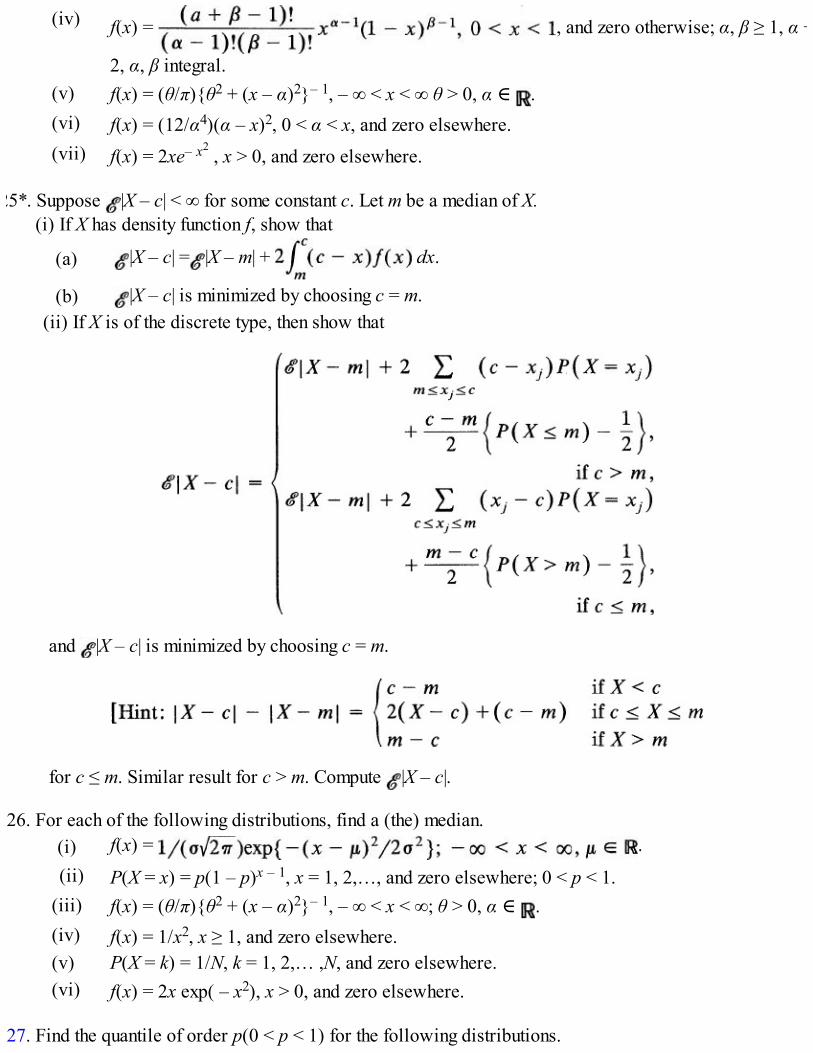
(iv) f(x) = , and zero otherwise; α, β ≥ 1, α +

2, α, β integral.(v) f(x) = (θ/π){θ2 + (x – α)2}– 1, – ∞ < x < ∞ θ > 0, α ∈ .(vi) f(x) = (12/α4)(α – x)2, 0 < α < x, and zero elsewhere.(vii) f(x) = 2xe– x2 , x > 0, and zero elsewhere.

25*. Suppose |X – c| < ∞ for some constant c. Let m be a median of X.(i) If X has density function f, show that

(a) |X – c| = |X – m| + dx.

(b) |X – c| is minimized by choosing c = m.(ii) If X is of the discrete type, then show that

and |X – c| is minimized by choosing c = m.

for c ≤ m. Similar result for c > m. Compute |X – c|.

26. For each of the following distributions, find a (the) median.(i) f(x) = .(ii) P(X = x) = p(1 – p)x – 1, x = 1, 2,…, and zero elsewhere; 0 < p < 1.

(iii) f(x) = (θ/π){θ2 + (x – α)2}– 1, – ∞ < x < ∞; θ > 0, α ∈ .(iv) f(x) = 1/x2, x ≥ 1, and zero elsewhere.(v) P(X = k) = 1/N, k = 1, 2,… ,N, and zero elsewhere.(vi) f(x) = 2x exp( – x2), x > 0, and zero elsewhere.

27. Find the quantile of order p(0 < p < 1) for the following distributions.

(i) f(x) = 1/x2, x ≥ 1, and zero elsewhere.(ii) f(x) = 2x exp( – x2), x ≥ 0, and zero otherwise.

(iii) f(x) = 1/θ, 0 ≤ x ≤ θ, and zero elsewhere.(iv) P(X = x) = θ(1 – θ)x – 1, x = 1, 2,…, and zero otherwise; 0 < θ < 1.(v) f(x) = (1//β2)x exp(– x/β, x > 0, and zero otherwise;(vi) f(x) = (3/b3)(b – x)2, 0 < x < b, and zero elsewhere.

28*. Let x1, x2,… ,xn be n real numbers. Set and – 1). Let k ≥ 1.

Show that the fraction of x1,…, xn included in the interval ( – ks, + ks) is at least 1 – 1/k2.

29. If X is symmetric about a, show that α is the median of X.

3.8 RANDOM SAMPLING FROM A PROBABILITY DISTRIBUTION

Consider the disintegration of radioactive elements (Example 1.2.3). Recall that the rate of decay of aquantity of a radioactive element is proportional to the mass of the element. That is,

where λ > 0 is a constant giving the rate of decay and m is the mass of the element. Integrating withrespect to t we see that

where c is a constant. If m = m0 at time t = 0 then c = ln m0 and

Given m0 and λ we know m as a function of t. The constant λ is the parameter of the relationship (2) inthe sense that for any particular choice of λ > 0 we obtain a specific exponential relationship between mand t.

If, on the other hand, the time X at which the element disintegrates is considered to be random wewould be interested in the probability that a given element will decay before time t. In order to computethis probability we need to have a suitable model for the density of X. Note that the fraction of the originalmass m0 that decays in [0, t] is given by

which may be taken as P(X ≤ t) for t > 0. That is, we take

which gives the density function of X as

Define f(t) = 0 for t ≥ 0. Again, λ > 0 is a parameter of this stochastic or nondeterministic model ofradioactive decay in the sense that a particular choice of λ > 0 gives a specific density of X and a specificprobability P(X ≤ t). (See also Section 4.2.) For now, we think of parameters as numerical quantitiesassociated with a probability distribution. Thus, the mean and the variance (if they exist) and also thequantiles of a distribution are all parameters.

We recall that the basic difference between probability theory and statistical inference is that in theformer one specifies a model and studies its consequences (what is the probability that an element willdecay by time t?) whereas in the latter the model is not completely known. The object, then, is todetermine some properties of the model (underlying distribution of X) on the basis of observed data. Inthe example considered above this means, in particular, to make a guess at the unknown value of λ(estimation) or perhaps to settle the validity of a less precise statement about λ such as λ ≤ λ0 (testing ofhypothesis). Often, however, even the functional form of the distribution of X is not known. (See Chapter4 for more details.)

The basic statistical technique used in statistical inference is to replicate the experiment under (moreor less) identical conditions, thus obtaining what is called a random sample. In the example underconsideration this means that we take repeated and independent observations on X, say x1, x2,…, xn.These observations may be regarded as values of random variables X1, X2,… ,Xn respectively where X1,X2,…, Xn have the same distribution and are independent.

DEFINITION 1. Two random variables X and Y are said to be identically distributed if they have the same distribution function.

We emphasis that if X and Y are identically distributed it does not follow that P(X = Y) = 1. (SeeProblem 3.) It is clear that the Xi’s need to have the same distribution if they are to represent replicationsof the same experiment. Independence is used to specify the joint distribution of the sample.

DEFINITION 2. Let X1, X2,…, Xn be independent and identically distributed with common distribution function F. We say that X1,X2… , Xn is a random sample from F.

If X1, X2,…, Xn is a random sample from a distribution function F, then the joint distribution of X1,…,Xn is given by

if F has density function f and by

when X1, X2,…, Xn are of the discrete type with common probability function P(X1 = xj). Sometimes the

term population is used to describe the universe from which the sample is drawn; the population may beconceptual (see Remark 3 below). Often F is referred to as the population distribution.

Remark 1. In sampling from a probability distribution, randomness is inherent in the phenomenonunder study. The sample is obtained by independent replications. In sampling from a finite population, onthe other hand, randomness is a consequence of the sampling design. We recall that in sampling from afinite population of N elements, a sample of size n is said to be a (simple) random sample if each of the

possible samples has the same chance of being selected (in sampling without replacement and

without regard to order).

Remark 2. Sampling from a probability distribution is sometimes referred to as sampling from aninfinite population, since one can obtain samples of any size one wants even if the population is finite (bysampling with replacement).

Remark 3. In sampling from a finite population, the term population is meaningful in that it refers tosome measurable characteristic or characteristics of a group of individuals or items. When the populationis not finite it is often difficult to identify an underlying population. This happens, for example, in cointossing or rolling a die, or when measurements involve a manufacturing process (such as life length of alight bulb or net weight of coffee in 10 oz. coffee jars). In these cases the sample is generated by anongoing random phenomenon.

Remark 4. We can also think of a random sample as an outcome of a (composite) random experiment whose outcomes are n-tuples (x1, x2,…, xn). Then xi may be thought of as the outcome of a component

random experiment i of . In general, given a composite random experiment with components i andthe joint probability distribution of , we can always compute the probability distribution of i (bytaking the marginal distribution). In the case of random sampling from a probability distribution, however,the probability distribution of determines and is completely determined by that of any i.(See alsoSection 2.7)

Example 1. Number of Girls in a Family of Five Children. Assuming that both sexes are equally likely, the number of girls X in arandomly selected family of five children has probability function

(see Section 6.3). A random sample of n families (with five children) showed x1, x2, …, xn girls. Then the probability of observing thissample is given by

for 0 ≤ xj ≤ 5, j = 1, 2,…,n. In a random sample of size n = 3, the probability that x1 + x2 + x3 ≤ 1 is given by

That is, in a sample of three families the probability is .0005 that one will observe a total of at most one girl. The probability that each ofthe three sampled families will have at most one girl is given by

Example 2. Reliability of Electrical Parts. In studying the reliability of electrical parts, the lifetime X (in hours) of a given part canbe assumed to be a random variable with density function

A random sample of n parts is put to test. Then the joint distribution of the sample X1, X2,…, Xn is given by:

for x1 ≥ 0, x2 ≥ 0, …, xn ≥ 0, and zero elsewhere. Here θ > 0, β > 0 are parameters either or both of which may be unknown. Theprobability that each part will survive t hours is given by:

Now

so that

If β, θ are known, this probability can be evaluated. If either θ or β or both are unknown, then the problem (of statistical inference) may beto estimate the unknown parameters from the data x1, x2,… ,xn or to estimate the probability P(X1 > t,…, Xn > t).

Sample Statistics

In practice we often observe a function of the sample. When we toss a coin n times we hardly, if ever,keep track of the result of each trial. Rather, we count the number of heads (or equivalently the number oftails) in n trials. Let X1, X2,…,Xn be a random sample. Then any function (X1, X2,…, Xn) that can becomputed from the sample without the knowledge of values of the unknown parameters is given a specialname.

DEFINITION 3. Let (X1, X2,…,Xn) be a random vector. Then a statistic ϕ(X1, X2,…,Xn) is an observable function of the observationvector (X1, X2,…,Xn). That is, the statistic ϕ is directly computable from the data vector (X1, X2,…, Xn). A statistic ϕ may be univariateor multivariate.

We note that a statistic is an alternative name given to a random variable (or random vector) when wehave a sample of observations. In practice X1, X2,…, Xn will be a random sample, that is, X1, X2,…, Xnwill be independent and identically distributed.

Example 3. Sample Mean and Sample Variance. Let X1, X2,…, Xn be a random sample from a distribution function F. Then twosample statistics of great importance in statistics are the sample mean defined by

and the sample variance defined by

The statistic ( , S2) is usually referred to as a joint statistic. Note that we divide by (n – 1) and not n in (5) for reasons that will become

clear later. Moreover, both and S2 are always finite irrespective of whether the population mean and variance do or do not exist. Someother statistics of interest are max( X1, X2,…, Xn), min( X1, X2,…,Xn), median, and mode of the sample.

In particular, let X denote the number of children in a family. Suppose a random sample of 10 families shows the following values of X:

5 0 3 2 1 4 3 2 2 3

Then

and

Sometimes the following computational formula for S2 is useful

The positive square root S of S2 is known as the sample standard deviation. We note that for a specific set of observed values (x1, x2,

…,xn) of (X1, X2,…,Xn) we use the notation and s2 for the corresponding values of and S2. This is consistent with our conventionof using lower-case letters to denote values of a random variable.

We remark that sample statistics are simply the numerical characteristics of the sample just asparameters are numerical characteristics of the population. However, sample statistics are randomvariables and vary from sample to sample, whereas parameters are fixed constants. The following tablesummarizes some facts about parameters and statistics.

According to Problem 3.7.28, an analog of the Chebyshev’s inequality holds for each sample x1, x2,…,xn.

Example 4. Proportion of Defective Parts In a Sample. The length X (in centimeters) of a manufactured part may be considered tobe a random variable. A random sample of 25 parts showed a mean of 1.01 cm with a standard deviation of .01 cm. If a manufacturedpart is considered defective when its length is ≤ .99 cm or ≥ 1.03 cm, what proportion of the sample parts is defective?

In the absence of any information about the distribution of X we cannot compute the probability P(.99 < ≤ 1.03) or P( ≤ .99 or ≥ 1.03). We can, however, use Chebyshev’s inequality to get an upper bound on the proportion of defective parts in the sample. From

Problem 3.7.28 we recall that the proportion of sample values included in the interval ( – ks, + ks) is at least 1 – 1/k2. Since – ks =1.01 – k(.01) = .99 we see that k = 2. Hence at most a proportion 1/k2 = .25 of the 25 parts in the sample is defective.

Example 5. Reliability of Electrical Parts (Example 2). In Example 2 the lifetime in hours of an electrical part was assumed tohave density function

What is the probability that a random sample of size n = 2 will produce an average life-length of t hours or more? Here we wish toevaluate P( ≥ t) where = (X1 + X2)/2. For convenience we take β = 1. We have

Figure 1

Remark 5. (Sample Median and Sample Mode). Let x1, x2,…,xn be a random sample. Then a samplemode is a value that occurs most often. In Example 3, there are two sample modes. Family sizes 2 and 3occur three times each and are modal family sizes. A sample median is a value that divides the sampleinto two equal parts, each part containing at least half the values. In order to compute a sample median wearrange x1, x2,…,xn in increasing order, say, x(1) ≤ x(2) ≤ … ≤ x(n). If n is an odd integer then there is

exactly one middle value, namely x((n + 1)/2), which then is a median. If n is even, then there are twomiddle values x(n/2) and x((n/2) + 1. Then any x, x(n/2) < x < x((n/2) + 1 is a median. Usually one takes theaverage (x(n/2) + x(n/2 + 1))/2 as a median. In Example 3, the ordered arrangement is

Since n = 10, the two middle values are 2 and 3 and we take (2 + 3)/2 = 2.5 as the sample median. Amore formal discussion of sample quantiles appears in Section 8.5.

Remark 6. (Infinite Number of Random Variables). We conclude this section with some commentsconcerning an infinite number of random variables. In the later chapters we shall be often concerned withsome properties of an infinite sequence of random variables. The question that we need to answer is thefollowing: How do we specify a probability model for this sequence of random variables? That is doneby specifying the joint distribution of (X1, X2,…,Xn) for every positive integer n. That is, in order tospecify a probability model for an infinite sequence {Xn} we need to specify the joint probabilities

where A1, A2, A3,… respectively are events in 1, 2, 3,…. We emphasize that we cannot arbitrarilydefine the successive joint distributions. If we know the joint distributions of (X1, X2,…,Xn + 1), then the(marginal) joint distribution of (X1,…, Xn) is obtained by letting Xn + 1 take on all possible values. Hencethe successive joint distributions must satisfy this consistency property. In the special case when X1, X2,… are independent and identically distributed, the case of most interest to us, the specification of themarginal distribution F of X1 suffices since in that case the joint distribution function of (X1,…, Xn) forevery n is the product of the marginal distribution functions of X1, …, Xn each of which is F.

Problems for Section 3.8

1. Transistors have a life length that has the density function

A random sample of 5 transistors is taken and their time to failure is recorded. What is the jointdensity function of the sample?

2. A random sample of size n is taken from the probability function

What is the joint probability function of the sample?

3. A fair coin is tossed once. Let X be the number of heads and Y the number of tails. Are X and Yidentically distributed? Is P(X = Y) = 1?

4. A fair coin is tossed eight times. Each time a head is observed we write 1, and 0 (zero) otherwise.

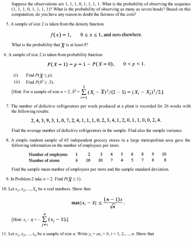
Suppose the observations are 1, 1, 1, 0, 1, 1, 1, 1. What is the probability of observing the sequence(1, 1, 1, 0, 1, 1, 1, 1)? What is the probability of observing as many as seven heads? Based on thiscomputation, do you have any reason to doubt the fairness of the coin?

5. A sample of size 2 is taken from the density function

What is the probability that is at least.9?

6. A sample of size 2 is taken from probability function

(i) Find P( ≤ p).(ii) Find P(S2 ≥ .5).

[Hint: For a sample of size n = 2, S2 = .

7. The number of defective refrigerators per week produced at a plant is recorded for 26 weeks withthe following results:

Find the average number of defective refrigerators in the sample. Find also the sample variance.

8. A simple random sample of 65 independent grocery stores in a large metropolitan area gave thefollowing information on the number of employees per store.

Find the sample mean number of employees per store and the sample standard deviation.

9. In Problem 2 take n = 2. Find P( ≥ 1).

10. Let x1, x2,…, Xn be n real numbers. Show that:

[Hint: xi – = – .

11. Let x1, x2,…, xn be a sample of size n. Write yi = axi + b, i = 1, 2,…, n. Show that

where is the mean of is the sample variance of the y’s and is the sample varianceof the x’s.

12. The weights (in kilograms) of five bags of navy beans were recorded to be: 1.1, 1.3, 0.9, 1.2, 1.0.(i) What is the sample mean and the sample variance?

(ii) What is the sample mean and the sample standard deviation if the weights were recorded inpounds?

[Hint: One kilogram 2.2 pounds. Use the result of Problem 11.]

13. A random sample of 25 I.Q. scores given to entering freshman at a state university showed a mean of125 with a standard deviation of 13.2.

(i) Find an interval in which at least 75 percent of the I.Q. scores lie.

(ii) Give an upper bound for the proportion of students in the sample whose I.Q. score on the test is atleast 150.

[Hint: Use Chebyshev’s inequality of Problem 3.7.28.]

14. Let x1, x2,…,xn be a set of n real numbers. Let x(n) = max{x1, x2,…, xn} and x(1) = min{x1, x2,…, xn}.

Show that for any set of real numbers a1, a2,… an such that the following inequality holds.

[Hint: any constant c. Use triangular inequality and choose c

appropriately.]

15. Show that X has a symmetric distribution if and only if X and – X are identically distributed.

16*. Let X1, X2 be a random sample from a continuous distribution which is symmetric about θ. That is, if fis the common density of the Xi’s, then

(i) Show that

for all x, so that the distribution of X1 + X2 is symmetric about 2θ. (By induction one can show thatthe distribution of X1 + ··· + Xn is symmetric about nθ.)(ii) Show that

for all x ∈ so that the distribution of X1 – X2 is symmetric about 0.

3.9 REVIEW PROBLEMS

1. Which of the following functions are density functions? Find the corresponding distribution functionwhenever the function defined below is a density function.(i) f(x) = sin x, 0 ≤ x ≤ π/2, and zero elsewhere.(ii) f(x) = (1/2)|sin x|, |x| < π/2, and zero elsewhere.

(iii) f(x) = x/4 for 0 ≤ x ≤ 1, = 5/8 for 1 ≤ x < 2, = (3 – x)/2 for 2 ≤ x < 3, and zero elsewhere.(iv) f(x) = (1/24)x(1 – x/12), 0 ≤ x ≤ 12, and zero otherwise.(v) f(x) = (1/4θ) if 0 < x < θ/2 or 3θ/2 ≤ x ≤ 2θ, = 3/(4θ) if θ/2 < x < 3θ/2, and zero elsewhere.(vi) f(x) = (1/2θ)cos (x/θ), –πθ/2 ≤ x ≤ πθ/2 and zero otherwise.

2. Are the following functions distribution functions? If so, find the corresponding probability ordensity functions.(i) F(x) = 0, x < 0, and = 1 – exp(– x2/2σ2) if x ≥ 0; σ > 0.(ii) F(x) = 0 if x ≤ 0, = In x if 0 < x ≤ 2, and = 1 if x > 0.

(iii) F(x) = 0 if x < 1, = In x/ln 2 if 1 ≤ x ≤ 2, and = 1 if x > 2.(iv) F(x) = 1 – exp(– xβ) if x ≥ 0, and zero elsewhere; β > 0.(v) F(x) = 1 – (2x + 1)e– 2x, for x ≥ 0 and zero otherwise.(vi) F(x) = 0 if x < 0, = 1/2 if 0 ≤ x < 1/2, = x if 1/2 ≤ x < 1, and = 1 if x > 1.

3. The number of arrivals X at a bank in any 15-minute period has probability function

Find:(i) P(X ≥ 1).(ii) P(X < 2).

(iii) P{X ≥ 1|X < 2}.

4. The storage capacity of jet fuel at an airport is 1.5 million gallons. Suppose the daily consumption(in million gallons) of jet fuel at this airport has density function given by

How often will the fuel run out by the end of the day if the tank is filled at the beginning of each day?

5. The percentage X of antiknock additive in a particular gasoline has density function

(i) Find c, X and var(X).

(ii) Find P(X ≥ 1/2).

6. The manufacturer of liquid fertilizer makes 89 profit on each gallon of fertilizer it sells in thesummer of the year it is manufactured. Amount not sold by the end of the summer is stored at a cost of25 per gallon. Suppose the demand X for his fertilizer has density function

V 106

At what level should he stock in order to maximize his average profit? What is the maximumaverage profit?

7. Let f1, f2,… fk be probability density functions on the interval (a, b).

(i) Show that cannot be a density function on the interval (a, b).

(ii) Show that , is a density function on (a, b).

8. Let X be a bounded random variable. That is, suppose there exists a constant c > 0 such that P(|X| ≤c) = 1. Show that |X| < ∞ and | X| ≤ c.

9. Suppose X has symmetric distribution about a point c and |X| < ∞. Show X = c.

10. Suppose P(X ≥ Y) = 1. Suppose |X| < ∞ and |Y| < ∞. Show that X ≥ Y and X = Y if and onlyif P(X = Y) = 1.

11. Let X be the amount (in thousands of dollars) of itemized deductions on a randomly selected federalincome tax return. Suppose X has density function

Here α > 1 is a constant.(i) Find mode if it exists.(ii) Find the quantile of order p, 0 < p < 1.

(iii) Find the median if α = 2.

12. Find the mean and the variance of the density functions in part (iv), (v) and (vi) of Problem 1.

13. Compare the probability bounds obtained from Chebyshev’s inequality in Problem Ω with the exactresults.

14. Suppose X has probability function given by

where c > 0 is a constant. Find the constant c and the mean and the variance of X.

15. A manufacturer counts major and minor defects in sump pumps it manufactures for quality controlpurposes. Suppose only four characteristics are inspected. Let X be the number of minor defects and Ythat of major defects in a sump pump. Suppose (X, Y) has joint probability function given by

(i) Find the two marginal distributions and the conditional distributions.(ii) Find P{ X ≥ 1|Y ≤ 3} and P{X ≤ 2|Y = 1}.

(iii) Find P(Y > X) and P(Y ≥ X).

16. Let (X, Y) have joint density function

(i) Are X and Y independent?(ii) Find P(|X – Y| > 1/2).

(iii) Find the marginal density of Y and the conditional density of X given Y = y.(iv) Find P{1/4 < X < 1/2|Y = 3/8} and P{1/4 < X < 1/2|1/4 < Y < 3/8}.

17. Let X and Y be the times to failure of two batteries and suppose X and Y are independent withrespective densities

Find P(X – Y > 0) and P(|X – Y| > 2)

18. Three points X1, X2, and X3 are randomly selected from the interval (0,1)(i) Find the probability that exactly two of the points selected will be ≥ .60.(ii) Find the probability that X1 + X2 > X3.

19. A random sample of size 2 is taken from the density function

What is the probability that the sample variance will be greater than λ2/2?

20. A random sample of size two is taken from the probability function

What is the probability that the sample variance will be at least as large as the sample mean?

† This is a gamma integral, to be studied in Section 7.3.

† Recent work has shown that although this inequality is well known in the literature as Chebyshev’s inequality it is also due to I. J. Bienayme.

CHAPTER 4

Introduction to Statistical Inference

4.1 INTRODUCTION

Given a random experiment, we have constructed a stochastic model for the experiment by identifying aset of all outcomes Ω, the events of interest A, A ∈ ζ, and by assigning to each event A a probability P(A).We then translated the problem to the real line (or n) by defining a random variable (or a randomvector) X on Ω. We saw that X induces a probability distribution Px on events E in this new sample spacethrough the correspondence

We showed that Px can be specified simply by specifying the distribution function, or the density orprobability function, of X.

Suppose we have n observations x1, x2, …, xn on some random variable X. What information does itcontain about the distribution F of X? How does it help us to make a guess at F or some numericalfunction of F? The answer depends on the type of assumptions we are willing to make about F. If wemake little or no assumptions about F, then the family of possible distributions of X is callednonparametric. On the other hand, if we assume that the form of F is known except for some numericalvalues of a finite number of constants (parameters) θ1(F) , θ2(F),…, θk(F), then the family of possibledistributions of X is called parametric. Section 4.2 gives formal definitions of these two concepts andprovides some typical examples of parametric and nonparametric inference problems.

Often the problem of inference is to make a guess at the numerical value of some constant(s) θ(F). InSection 4.3 we consider the problem of estimating θ(F) by a point estimate. We explore some desirableproperties of a point estimate of θ(F). Sometimes it is preferable to estimate θ(F) by an interval (or a set)of values that includes the true θ(F) with a large prespecified probability. This so-called problem ofconfidence estimation is also considered in Section 4.3.

In earlier chapters we often computed P(T(X1, X2,…, Xn) ∈ A) where T(X1, X2,…, Xn) is a samplestatistic. The numerical value of this probability was then used to assess the strength of argument that thesample data provides for or against our underlying model assumptions. This, however, is not enough. Wealso need to contend with the probability P(T(X1, X2,…, Xn) ∈ A) computed under the assumption that themodel is false. Suppose, for example, that P0 and P1 are the two contending probability models for theunderlying distribution of the Xi’s. How do we choose between P0 and P1? This so-called problem ofhypothesis testing is the subject of investigation in Section 4.4. The close relation between confidenceestimation and hypothesis testing is also explored.

In Section 4.5 we consider some simple graphic methods of looking at the data. Methods of estimatingthe distribution function and probability or density function are also introduced. The shape of the graph ofthe estimate of probability or density function can often be used to see if the sample could have come froma known family of distributions.

4.2 PARAMETRIC AND NONPARAMETRIC FAMILIES

Let (X1, X2,…, Xn) be a random vector from a joint distribution function G. A specification of thestochastic model governing the observations requires a specification of the set of all possible jointdistribution functions G for the Xi’s. How is the family selected? As much as one would like to belarge in order that no possible underlying distribution for the Xi’s is excluded, it is not realistic to expectthat one realization (x1, x2,…, xn) will tell us anything about the specific G ∈ . Since the object isusually to predict future performance when replications of the same experiment are made, it is reasonableto limit by assuming that X1, X2,…, Xn are independent, identically distributed, and have a commondistribution function F. That is, X1, … , Xn is a random sample from F so that

It is then sufficient to consider univariate distribution functions F ∈ say. If we restrict still further by specifying the form of F, we should be able to get fairly detailedinformation on the specific F ∈ from the sample (x1,…, xn). However, taking too small may lead toexclusion of the true F and hence wrong conclusions.

It is convenient to distinguish between parametric and nonparametric families of distributions becausethe methods used in two cases differ greatly. In a parametric model, we specify the form of thedistribution (through its density or probability function) with the exception of the index or parameter θwhere θ belongs to a parameter set Θ that is a subset of a finite dimensional Euclidean space. Thus weget all distributions in by varying at most a finite number of scalar parameters whose values completelydetermine a unique member of .

Example 1. Model for Coin Tossing. Suppose a coin is tossed n times. Let Xi = 1 if the ith toss results in a head and zero otherwise,and let P(Xi, = 1) = p = 1 – P(Xi = 0). If we know n, then a specification of p determines precisely one distribution for the number of heads in n trials. Here p is the parameter that is scalar, and Θ = {0 ≤ p ≤ 1} is the parameter set. On the other hand, if wemake m observations Y1, Y2,…, Ym on the Y’s without the knowledge of n and p, then the parameters are n and p so that θ = (n, p) andΘ = {(n, p): n = 1, 2,… ,0 ≤ p ≤ 1}. If we specify the numerical values of both n and p, we know precisely the distribution that governsthe y’s.

Example 2. Survival Times of Patients with Advanced Lung Cancer. Suppose 100 patients with advanced lung cancer arefollowed until their death. Let X1, X2,…, X100 be their survival times. If we assume that the survival times can be modeled according tothe density function

then the parameter θ is scalar with θ ∈ Θ = (0, ∞). All possible distributions for the Xi’s can be obtained by varying θ in Θ, and aspecification of the numerical value of θ completely specifies the underlying density of the Xi’s.

It is clear, then, that we need a dictionary of some well-known and frequently used models as well asa listing of their properties, which will help facilitate our choice of an appropriate parametric model forthe random phenomenon under study. This is done in Chapters 6 and 7.

Often, however, we do not have enough information to rely on a specific parametric model. In thatcase we may consider a much wider class of distributions. In a nonparametric model, the family ofunderlying distributions for X is so wide that cannot be indexed by a finite number of numericalparameters. Thus a specification of a finite number of numerical parameters does not uniquely determine amember of .

The terms “nonparametric” and “distribution-free” are used interchangeably. It should be noted,however, that “nonparametric” does not mean that there is no parameter and distribution-free does notmean that no distributions are involved.

Example 3. Family of Distributions with Finite Mean. Let be the family of all distribution functions on the real line that havefinite mean. This is a very large class of distribution functions, and no matter how many scalar parameters are specified we cannot ingeneral specify the specific F in that governs the observations. Hence is classified as a nonparametric family.

Example 4. Symmetric Distributions. Let be the set of all distributions on the real line that are symmetric about their median.Again is a nonparametric family since it cannot be characterized by a finite set of scalars.

In nonparametric statistics, the most that we will assume (unless otherwise specified) is that theunderlying distribution is of the continuous type. This is a mathematically convenient assumption thatallows us to assume that the observations can be arranged in increasing (or decreasing) order with no ties[for continuous-type random variables P(X = Y) = 0]. This family is so wide that in general theprocedures used will not be as sharp and powerful as those developed for a narrowly defined parametricfamily. At times, however, the nonparametric procedures are almost as good as the parametric ones. Thepoint is that before we apply any parametric procedure we must make sure that the underlyingassumptions are satisfied, or at least reasonably satisfied. If it is felt that there is not enough informationavailable to choose a specific parametric model, it is advisable to use a nonparametric procedure.

Problems for Section 4.2

In each of the following cases, determine whether you will classify the family of distributions asparametric or nonparametric.

1. = {f : f is a density satisfying f(x) = f(–x)}.

2. = {Pλ(x) = e–λλx/x!; x = 0, 1,…; λ > 0}.

3. = {F: F is a continuous distribution function or has only jump discontinuities}.4. = {f: f is a density with unique median}.5. = {fθ(x) = 1/θ, –θ/2 < x < θ/2, zero otherwise, θ > 0}.

6.

7. and zero elsewhere, μ ∈ , θ > 0}.8. = {PN(x) = 1/N, x = 1, 2,…, N; N ≥ 1}.

9. = {f: f is unimodal density}.10. and zero elsewhere; α ≥ 1 is an integer, β >

0}.

In the following problems construct an appropriate statistical model for the experiment. Identify g, theparameter, and the parameter set.11. A die is tossed repeatedly. The object is to decide whether the die is fair or loaded. A record is kept

of the number of l’s, 2’s, 3’s, 4’s, 5’s, and 6’s that show up in n trials.

12. A manufacturer produces 1-inch wood screws, some of which go unslotted. A random sample of nscrews is taken from a very large batch to see whether the overall proportion of unslotted screws issufficiently small.

13. A manufacturer of 12-volt automobile batteries takes a sample of size n from a large lot and measuresthe length of life of each battery.(i) The object is to estimate the overall proportion of batteries that do not meet the given

specification (length of life greater than a prespecified number of hours).(ii) The object is to estimate the average length of life of batteries it produces.

4.3 POINT AND INTERVAL ESTIMATION

Suppose a decision has been made concerning the model, whether nonparametric or parametric. How dowe estimate a parameter or some parameters of the model? How accurate is this estimate? That is, howdo we measure the precision of our estimate? In order to motivate discussion, suppose we wish to find theaverage survival times of patients with advanced lung cancer. Let X denote the survival time of arandomly selected patient, and suppose F is the distribution function of X. We take a sample of n patientsand follow them until their death. Let X1, X2,…, Xn be the survival times of the n patients. How do we usethe observations X1, X2,…, Xn to estimate † This very much depends on the assumptions weare willing to make about F. If we assume only that F ∈ where is the family of all continuousdistribution functions on the real line with finite mean, then is a nonparametric family of distributions.In this case the form of F is unknown and hence cannot be used. If, on the other hand, it is felt that thedensity

adequately describes the distribution, then is a parametric family with parameter β belonging to theparameter set Θ = (0, ∞). In this case μF = FX = β so that the problem reduces to estimating β. Once β isknown, the distribution F is completely known. (In the nonparametric case, knowledge of μF tells us littleabout the distribution function F.)

We have so far been using the word “estimate” in its dictionary sense. Let us now make a formaldefinition.

DEFINITION 1. (POINT ESTIMA TE). Let (X1, X2,…, Xn) be a random vector with joint distributionfunction F ∈ . Let θ = θ(F), F ∈ be the (scalar or vector) unknown parameter of interest which takesvalues in Θ = {θ(F): F ∈ }. Any statistic T(X1, X2,…, Xn) is said to be a (point) estimate of θ if it cantake values only in Θ.

Some remarks are in order. First, we note that the statistic T must be observable (that is, computablefrom the sample). Hence it cannot be a function of any unknown parameter. Next, we note that frequently adistinction is made between an estimate and an estimator. This distinction is the same as that between arandom variable and a value assumed by it. An estimator is the statistic used to estimate the parameter,and a numerical value of the estimator is called an estimate. For notational convenience, we will notfollow this distinction. Third, even though all statistics that take values in Θ are possible candidates forestimates of θ, it is clear that we have to develop criteria that indicate which estimates are “good” and

which may be rejected out of hand. Certainly estimates that are constants (not based on the observations)should not be admissible under any reasonable criteria (except for pedagogical reasons).

Example 1. Point Estimate for Median of a Distribution. Let X1, X2,…, Xn be a random sample from a continuous distribution thatis symmetric about its midpoint. This means that X1, X2,…, Xn are independent random variables, each having a common continuousdistribution function F(x) = P(X ≤ x), which is assumed to be symmetric about its midpoint or median mF (assumed unique):

This is clearly a nonparametric situation with θ = mF ∈ Θ = . Some reasonable estimates of mF are

(i) median of X1, X2,…,Xn,

(ii) (min Xi + max Xi)/2.

Of course there are infinitely many estimates to choose from since every real valued function of the sample is an estimate. However,often the choice narrows down to a few or at least to a manageable subset of the set of all estimates.

If, on the other hand, it is determined that the model can be narrowed down to the family of parametric density:

where θ ∈ is unknown, then the choice of estimates of θ (the median) is focused owing to the knowledge of the form of F or itsdensity. Some reasonable estimates of θ are: (i) (ii) median of X1, X2,…, Xn. The reason for choosing X is that θis also the mean of f. Moreover, as we shall see in Section 5.4 for large n, X is likely to be near θ. The estimate X has several otherimportant properties. The choice of median of X1,…, Xn as an estimate derives from the fact that θ is also the median of f.

Example 2. Estimating the Mean of a Distribution. Let X1, X2,…, Xn be a random sample from a distribution function F ∈ where is the class of all distributions on the real hne with finite mean μF. Suppose nothing else is assumed about F. Then the family is nonparametric. A reasonable estimate of μF is the sample mean

We will show in Section 5.4 that for large n, X is likely to be near μ, moreover X = μF (see Section 5.3). On the other hand, if it is felt,say, that the uniform distribution on [0, θ], θ > 0, adequately represents F, then the knowledge of the form of F can be used to constructother reasonable estimates of the mean (= θ/2). For example, in addition to X two other reasonable estimates are the sample median andone half the largest observation. All these estimates tend to be near θ for large n.

Remark on Notation 1. Let θ ∈ Θ be the unknown parameter to be estimated based on the sample X1,X2,…, Xn of size n. Estimates will usually be denoted by (X1, X2,…, Xn) = (with or without subscriptsdepending on the number of estimates under consideration). Whenever a Greek or other letter appearswith a “hat” above it, such as , , , it is assumed to be an estimate of the corresponding parameter(without hat).

We now turn our attention to two related problems in point estimation. How do we judge the worth orprecision of an estimate? What are some desirable properties that we may require our estimate topossess? Requiring an estimate to possess a certain desirable property restricts the search to a smaller setof estimates, whereas a measure of precision of an estimate helps us to choose between two (or more)estimates having the same property. Neither provides a constructive procedure for finding estimates.

Precision usually means some measure of “nearness.” How close is the estimate to the parameter? If

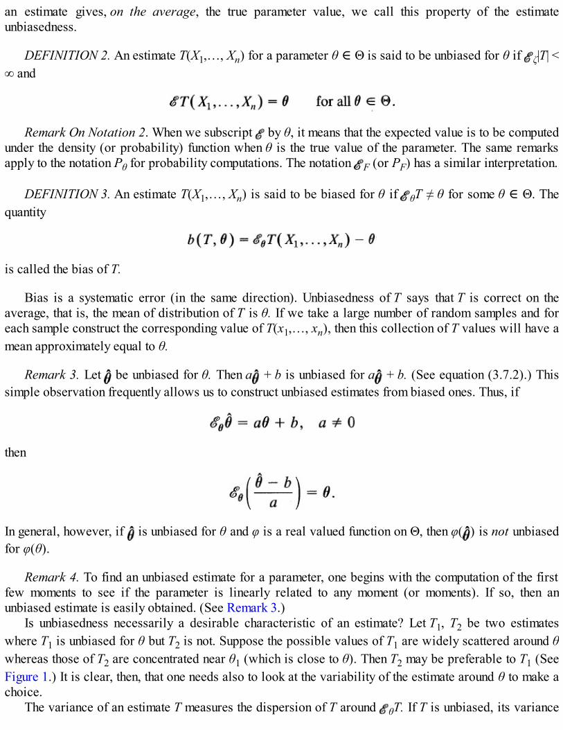
an estimate gives, on the average, the true parameter value, we call this property of the estimateunbiasedness.

DEFINITION 2. An estimate T(X1,…, Xn) for a parameter θ ∈ Θ is said to be unbiased for θ if ζ|T| <∞ and

Remark On Notation 2. When we subscript by θ, it means that the expected value is to be computedunder the density (or probability) function when θ is the true value of the parameter. The same remarksapply to the notation Pθ for probability computations. The notation F (or PF) has a similar interpretation.

DEFINITION 3. An estimate T(X1,…, Xn) is said to be biased for θ if θT ≠ θ for some θ ∈ Θ. Thequantity

is called the bias of T.

Bias is a systematic error (in the same direction). Unbiasedness of T says that T is correct on theaverage, that is, the mean of distribution of T is θ. If we take a large number of random samples and foreach sample construct the corresponding value of T(x1,…, xn), then this collection of T values will have amean approximately equal to θ.

Remark 3. Let be unbiased for θ. Then a + b is unbiased for a + b. (See equation (3.7.2).) Thissimple observation frequently allows us to construct unbiased estimates from biased ones. Thus, if

then

In general, however, if is unbiased for θ and φ is a real valued function on Θ, then φ( ) is not unbiasedfor φ(θ).

Remark 4. To find an unbiased estimate for a parameter, one begins with the computation of the firstfew moments to see if the parameter is linearly related to any moment (or moments). If so, then anunbiased estimate is easily obtained. (See Remark 3.)

Is unbiasedness necessarily a desirable characteristic of an estimate? Let T1, T2 be two estimateswhere T1 is unbiased for θ but T2 is not. Suppose the possible values of T1 are widely scattered around θwhereas those of T2 are concentrated near θ1 (which is close to θ). Then T2 may be preferable to T1 (SeeFigure 1.) It is clear, then, that one needs also to look at the variability of the estimate around θ to make achoice.

The variance of an estimate T measures the dispersion of T around θT. If T is unbiased, its variance

gives a good measure of its precision. If T is biased, we should still be looking at the variability of Taround θ as a measure of its precision.

DEFINITION 4. The mean square error (MSE) of an estimate T for θ is defined to be MSEθ(T) =

θ(T(X1,…,Xn) – θ)2.

We note (see Remark 3.7.4) that:

so that

that is, T is unbiased.Smaller MSE means greater precision. In comparing two estimates T1 and T2 of θ we choose the one

with smaller MSE. Thus, if

Figure 1

with strict inequality for at least one θ, then the estimate T1 is preferred over T2. Often this comparison ismade by considering the ratio MSEθ(T2)/MSEθ(T1).

DEFINITION 5. The relative efficiency (RE) of T1 in relation to T2 is defined by the ratio

Clearly, T1 is preferred over T2 if REθ(T1, T2) ≥ 1 with strict inequality for at least one θ.

Example 3. Estimating the Size of a Population. A box contains N (unknown) items marked 1 through N(≥ 2). We make oneselection from the box. How do we estimate N? This is a problem one encounters, for example, in estimating the number of taxis in atown. In World War II this problem was encountered by the Allies who wanted to estimate enemy production of tanks.

Let X be the observed number. Then

An obvious estimate of N is X, call it . Clearly X ≤ N. We have:

so that is biased. The bias is given by

Hence underestimates N, which is to be expected since we know that X ≤ N. The MSE of is given by:

where we have used the fact that

(A method of proving this last result for readers who are unfamiliar with it is suggested in Problem 6.2.1.)We note that although is not unbiased, is. In fact, since

is a linear function of N, we have:

Moreover,

Suppose, now, that we have n observations X1, X2,… , Xn on X. How do we estimate N? Since X = (N + 1)/2, and

, it is plausible that

so that N(2X – 1) = N. Then will be an unbiased estimate of N. Another estimate of N that we can use is =

max(X1, X2,…, Xn). Since ≤ N, we note that underestimates N and is a biased estimate of N. We consider the performance ofthese and some other estimates of N in Examples 6.2.1 and 10.4.3.

Example 4. Estimating the Average Number of Colds in a Year. Let X denote the number of colds that a person has in a year.Suppose the distribution of X can be adequately represented by the probability function

where λ > 0. Then Θ = (λ > 0} and we wish to estimate λ. Let us compute X. We have from Example 3.7.2 with t = 1 that X = λ. Itfollows that X is an unbiased estimate of λ. We leave the reader to show that the precision of X as an estimate of λ as measured by itsvariance is given by

We note that the estimate X takes the value 0 (which is not in Θ) with probability e–λ < 0.Suppose we take a random sample of size n. Let Xi be the number of colds that the ith person in the sample has in a year, i = 1, 2,…,

n. How do we estimate λ? Since λ = Xi we have said in Example 2 that X is a reasonable estimate of λ. Is X unbiased? That is, is λX= λ? Since and each Xi has mean λ, it is plausible that

This, however, is not a proof. The result is true, as we show in Section 5.3.

Example 5. Estimating θ2. Let Y be the tensile strength of a cable of diameter X mm. Suppose Y is proportional to X2. That is, Y =cX2 for some constant c. Let X have density function given by

What is an unbiased estimate of θ2?We note that if X is observed, then

It follows that

so that

Hence:

is an unbiased estimate of θ2.On the other hand, if Y is observed, then we can rewrite T in terms of Y as

which is unbiased for θ2.

Remark 5. In Examples 3, 4, and 5 we considered only parametric families and usually samples ofsize 1. This is because we have not yet defined expectations in the case of random vectors. We will showlater, for example, that X is always an unbiased estimate of μ (Example 2) and that its variance getssmaller as n gets larger (which is to be expected).

Remark 6. Sometimes Θ is an open interval but the estimate of θ takes values in the closure of Θ (seeExample 4). This awkward situation can sometimes be avoided by taking the parameter set to be theclosure of Θ.

Often it is desirable to estimate a parameter θ to within some prespecified deviation, ε. This cannotbe done with certainty because T(X1,…, Xn) is a random variable. However, one can compute

as a function of θ, ε, and n, and use it as a measure of closeness of T to θ.It is intuitively appealing to desire that as the sample size increases, the bias decreases. This need not,

however, be the case unless we also demand that the distribution of T tends to concentrate near θ withincreasing sample size. This property is called consistency: an estimate T is said to be consistent for θ iffor every ε > 0

as n → ∞. We emphasize that consistency is a property of a sequence of estimates and is a large sampleproperty. We note that in view of a simple extension of Chebyshev’s inequality (Problem 3.7.22) as n →∞ we have

provided MSEθ(T) → 0 as n → ∞. Some further aspects of consistency are explored in Section 9.5. Wecontent ourselves here with an example that demonstrates the amount of work we still need to do to usethese concepts with ease.

Example 6. Estimating Average Length of Life of a Fuse. Let X be the length of life (in hours) of a fuse manufactured by acertain process. Suppose the distribution of X is given by the density function

Then X = β (Example 3.7.5) and X is an unbiased estimate of β, the average life length. Suppose we take a random sample X1, X2,…,Xn of size n. Then the sample mean is a natural choice for an estimate of β. We will show that Xis in fact unbiasedfor β (Section 5.3). Is X consistent? That is, does

as n → ∞ for every ε > 0? In order to check this, we need to compute P(|X – β| > ε). This means that we need to compute the distributionof X. This is done in Chapter 8. Alternatively, we could use Chebyshev’s inequality and have

If var(X) → 0 (and it does) as n → ∞ we are through. The computation of var(X) is done in Section 5.3, and a general result concerningthe consistency of X for μ is proved in Section 5.4.

What about some other estimates of β? Let X(1) = min(X1, X2,…, Xn). That is, X(1)(ω) = min{X1(ω), X2(ω),…, Xn(ω)} for ω ∈ Ω.Then X(1) is a random variable (Section 8.5) and we will see that X(1) = β/n so that nX(1) is also an unbiased estimate of β. Is nX(1)consistent? We again need the distribution of nX(1). We will show (Section 8.5) that nX(1) has the same distribution as X, that is, nX(1)has density f given above, so that

Hence nX(1) is not consistent for β.

Example 6 demonstrates the types of problems a statistician encounters. These include judgmental aswell as mathematical problems. For example, which of the two estimates X and nX(1) is preferable? Sinceboth estimates are unbiased, we could use variance as a measure of their precision. We will see thatvar(X) < var(nX(1)) so that X is preferred if smaller variance is desirable. Both X and nX(1) are easilycomputed but in order to compute X we need the whole sample, whereas nX(1) can be computed themoment the first of the fuses under test fails. If time is of the essence, then nX(1) will have to merit seriousconsideration.

We have thus far given some basic definitions and some properties that we may want our estimate topossess. We have not considered any methods of estimation. In Chapter 10 we consider some methods ofestimation and properties of estimates they produce. Until then, what we have learned so far will besufficient.

We emphasize that we will concentrate mainly on some time-tested common methods of estimation. Inany particular situation, the choice of an estimate in particular and of a statistical procedure in general isgoverned by both statistical factors (such as validity of the procedure, reliability of the samplingprocedure used, and so on) and nonstatistical factors (such as simplicity, practical and economicimplications, and so on).

The problems at the end of this section deal primarily with the case of one observation even though inpractice one usually has a sample of size n > 1. We do this to avoid distributional problems of the typementioned in Example 6. The case n > 1 is considered in the following chapters.

Confidence Interval Estimation

It should be clear by now that a point estimate is meaningless without some measure of its precision. Onesuch measure we suggested above is to use the probability, P(|T – θ| ≤ ε), that T does not deviate from θby more than a prespecified ε. Since |T – θ| is the error in estimation, ε is an upper bound for error.Rather than specify the error in advance, we may wish to specify a lower bound for the probability: Whatis the error ε such that

Rewriting (6) as

we see that the question may be posed equivalently as follows. What is the interval that contains the true θwith a probability of at least 1 – α? From (7) we see that [T – ε, T + ε] is such an interval where e iscomputed from (6). An interval such as [T – ε, T + ε] is usually called a 1 – α level confidence intervalfor θ. The assertion is that the range of values [T – ε, T + ε] contains the true (but unknown) θ withprobability at least 1 – α. The quantity 1 – α is a measure of the degree of credibility of the interval.

Let [T – ε, T + ε] be a 1 – α level confidence interval for ε so that (7) holds. Then any interval I(T)that contains [T – ε, T + ε] is also a 1 – α level confidence interval for θ. Or, equivalently, any 1 – α levelconfidence interval is also a 1 – α′ level confidence interval for α′ > α. The length of a confidenceinterval is used as a measure of its precision. In general, we want our confidence intervals to be as smallas possible. Since the confidence interval is our estimate of the interval in which θ is located, the smallerthe interval the more precise the information about θ. These considerations motivate the followingdefinition.

DEFINITION 6. Let X1, X2,…, Xn be a random sample from a distribution function F ∈ and let θ =θ(F) be a numerical parameter. Let l(X1,…,Xn) and u(X1,…, Xn) be two statistics such that for all F ∈ F

Then the random interval [l(X1,…, Xn) , u(X1,…, Xn)] is known as a minimum level 1 – α confidenceinterval for θ. The quantity 1 – α is called the confidence level. If PF(θ ≤ u(X1,…, Xn)) = 1 – α we call u

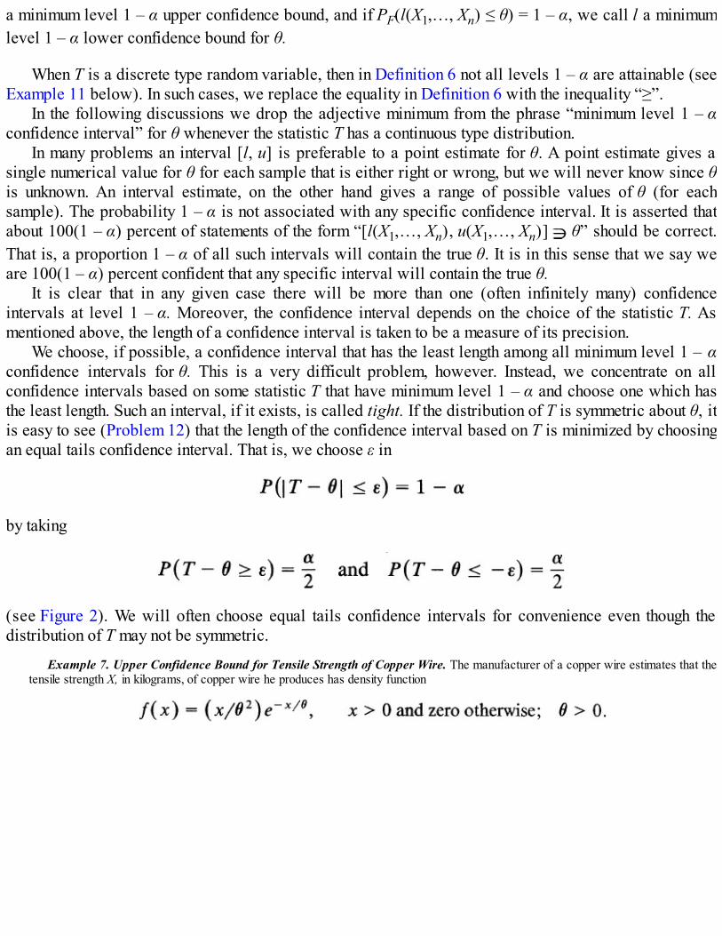
a minimum level 1 – α upper confidence bound, and if PF(l(X1,…, Xn) ≤ θ) = 1 – α, we call l a minimumlevel 1 – α lower confidence bound for θ.

When T is a discrete type random variable, then in Definition 6 not all levels 1 – α are attainable (seeExample 11 below). In such cases, we replace the equality in Definition 6 with the inequality “≥”.

In the following discussions we drop the adjective minimum from the phrase “minimum level 1 – αconfidence interval” for θ whenever the statistic T has a continuous type distribution.

In many problems an interval [l, u] is preferable to a point estimate for θ. A point estimate gives asingle numerical value for θ for each sample that is either right or wrong, but we will never know since θis unknown. An interval estimate, on the other hand gives a range of possible values of θ (for eachsample). The probability 1 – α is not associated with any specific confidence interval. It is asserted thatabout 100(1 – α) percent of statements of the form “[l(X1,…, Xn), u(X1,…, Xn)] θ” should be correct.That is, a proportion 1 – α of all such intervals will contain the true θ. It is in this sense that we say weare 100(1 – α) percent confident that any specific interval will contain the true θ.

It is clear that in any given case there will be more than one (often infinitely many) confidenceintervals at level 1 – α. Moreover, the confidence interval depends on the choice of the statistic T. Asmentioned above, the length of a confidence interval is taken to be a measure of its precision.

We choose, if possible, a confidence interval that has the least length among all minimum level 1 – αconfidence intervals for θ. This is a very difficult problem, however. Instead, we concentrate on allconfidence intervals based on some statistic T that have minimum level 1 – α and choose one which hasthe least length. Such an interval, if it exists, is called tight. If the distribution of T is symmetric about θ, itis easy to see (Problem 12) that the length of the confidence interval based on T is minimized by choosingan equal tails confidence interval. That is, we choose ε in

by taking

(see Figure 2). We will often choose equal tails confidence intervals for convenience even though thedistribution of T may not be symmetric.

Example 7. Upper Confidence Bound for Tensile Strength of Copper Wire. The manufacturer of a copper wire estimates that thetensile strength X, in kilograms, of copper wire he produces has density function

Figure 2

The average tensile strength is given by

A potential customer can use the wire only if the average tensile strength is not less than θ0. The customer decides to put a randomsample of n pieces of copper wire produced by the manufacturer to a test. Let x1, x2,…, xn be the tensile strengths of the n pieces in thesample. On the basis of this sample the customer would like to construct a lower confidence bound l(x1,…,xn) for the average tensilestrength 2θ at level 1 – α. If l θ0 then the customer should buy copper wire from this manufacturer. The problem, therefore, is to find astatistic l(X1,…, Xn) such that

Since X is a good estimate of X, we take T(X1,…, Xn) = X and find c > 0 such that

We have

Having found c as a function of θ we hope that we can invert the inequality X ≤ c to yield a lower bound for 2θ.Let us illustrate the computation for the n = 2 case. Anticipating a change of variable in the multiple integral, let us write c = kθ and

find k > 0 from

Thus k is a solution of

We note that g(k) = e–2k(4k3 + 6k2 + 6k + 3)/3 is strictly decreasing on (0, ∞) since g′(k) < 0 for all k. Hence g(k) = α has a uniquepositive solution. Given α, the equation can be solved numerically. In the following table we give the solutions for some selected values ofα.

For a given α let k1 > 0 be a solution of g(k) = α. Then for all θ > 0

It follows that the minimum level 1 – α lower confidence bound for X = 2θ based on X is given by l(X1, X2) = (X1 + X2)/k1.

Example 8. Confidence Interval for θ. Suppose X has density function

Let us find a 1 – α level confidence interval for θ based on a single observation. Given α, 0 < α < 1, our object is to find two randomvariables l(X) and u(X) such that for all θ > 0

We note that f is symmetric about the mean θ/2. Hence we can minimize the length of the confidence interval by choosing c = c(α) suchthat

In fact, c = θ(1 – α)/2. (See Figure 3.) We can rewrite (8) as follows:

so that [X/(1 – α/2), X/(α/2)] is a 1 – α level confidence interval for θ.

Figure 3

If, for example, the observation is 1.524 and α = .05, then the confidence interval for θ is [1.563, 60.96]. The assertion is not that theinterval [1.563, 60.96] contains unknown θ with probability .95. Indeed this interval, being fixed, either contains θ or it does not. Since θ isunknown, we will never know which of these two statements is correct. The assertion is that in sampling from density f, about 95 percentintervals of this type will contain the true θ. In Table 1 we demonstrate the result of taking 50 samples of size 1 from density f where θ isknown to be 1. Confidence intervals that do not contain θ = 1 are identified with an asterisk.

We note that 48 out of 50 intervals, or 96 percent, do contain the true value of θ.

TABLE 1. 95 Percent Confidence Intervals for θ

The inequality (6) invites comparison with Chebyshev’s inequality. Indeed if θT = θ then

Choosing we get

Letting 1 – α = 1 – 1/k2 we get k = 1/ so that for all θ ∈ Θ

If we are able to write the event

as

then [l(T), u(T)] is a 1 – α level confidence interval for θ.We note, however, that [ l(T), u(T)] is not a minimum level 1 – α confidence interval for θ. The level

is at least 1 – α. Since the Chebyshev’s inequality is crude, this method provides a rough and ready butfast confidence interval for the parameter. The length of such a confidence interval will usually be greaterthan the minimum level 1 – α confidence interval. The advantage, however, is that we do not need theunderlying distribution. All we need is varθ(T).

Example 9. Confidence Interval for θ of Example 8 Using Chebyshev’s Inequality.

Then X = θ/2 and var(X) = θ2/12. Choosing T(X) = 2X in (9) so that T is an unbiased estimate of θ we have

Hence (10) reduce to

Note, however, that for 0 < α < 1/3, 1 – (3α)–1/2 < 0 and 1 + (3α)–1/2 > 2. It follows that for 0 < α < 1/3 Chebyshev’s inequality leads tothe trivial confidence interval [X, ∞]. The length of this confidence interval is infinite, whereas the length of the confidence intervalconstructed in Example 8 was finite. If, on the other hand, α > 1/3 then the confidence interval is given by [2X/{1 + (3α)–1/2}, 2X/{1 –(3α)–1/2}]. We leave the reader to show that the length of this confidence interval is greater than the length of the confidence intervalconstructed in Example 8.

Example 10. Confidence Interval for Average Life Length. Let X be the length of life (in hours) of a fuse manufactured by acertain process. Suppose the distribution of X is given by the density

Then X = β and we seek a 1 – α level confidence interval for β.Let X1, X2,…, Xn be a random sample of size n from f. We need to find l(X1, X2,…, Xn) and u(X1, X2,…, Xn) such that

where 0 < α < 1. We have said that X is a good estimate of X1 = β. We therefore choose T(X1, X2,…, Xn) = X. Let us find c1 and c2,0 < c1 < c2, such that for all β > 0

We first note that this last equation has infinitely many solutions, each pair of solutions leading to a minimum level 1 – α confidenceinterval. Next we note that the density f is not symmetric about β or any other point. We therefore assign equal probability to each tail andchoose c1 and c2 from the equations

and

We now have a complicated problem of multiple integration. In Chapter 8 we show how to reduce these integrals to univariate integrals.We can then find c1 and c2 and invert the inequalities c1 ≤ X < c2 to yield a 1 – α level confidence interval for β.

Let us show how this can be done in the case when we have two observations. We use a simple trick here that is equivalent to achange of variables in the multiple integral. Instead of finding c1, c2 such that

let us find k1, k2 such that

In view of Example 3.8.5.

and

It follows that k1, k2 are solutions of the following equations

Given α, these equations can be solved numerically giving values of k1, k2. Note that the function g(x) = (1 + 2x)e–2x for x > 0 is strictlydecreasing since g′(x) < 0 for all x > 0. It follows that the equations

have unique solutions in (0, ∞). In the following table we have numerically computed k1 and k2 for some selected values of α.

Armed with the values of k1 and k2 we have for all β > 0

so that [X/k2, X/k1] is a 1 – α level confidence interval for βFor the case when we have exactly one observation, the problem is considerably simpler. In that case we find c1 and c2, 0 < c1 < c2,

such that

Once again we choose c1 and c2 by assigning equal probability to each tail. Thus we choose c1 and c2 from

so that

It follows that [– X/ln(α/2), – X/ln(1 – α/2)] is a 1 – α level confidence interval for β.In particular, if α = .10, then ln(α/2) = – 2.996, and ln(1 – α/2) = –.051 so that a 90 percent confidence interval is given by [X/2.996,

X/.051]. Intervals of this form will include the true (unknown) value of β for 90 percent of the values of X that we would obtain inrepeated random sampling from the density f. If, in particular, X = 207.5 is observed, then the confidence interval takes the value [69.26,4068.63].

Example 11. Confidence Interval for Probability of Heads. Consider a possibly biased coin with p = P(heads), 0 < p < 1. Ratherthan estimate p on the basis of n tosses of the coin, suppose we wish to estimate the interval in which p is located with probability 1 – α.For i = 1, 2,…, n let Xi = 1 if the ith trial results in a head and zero otherwise. Then is the proportion of successes in nindependent tosses of the coin. We have said that X is a good estimate of Xi = p. Therefore, we take T(X1,…, Xn) = X. Our object is tofind two statistics l and u such that

Since (X1,…, Xn) assumes only 2n values, both l and u assume at most 2n values each. Clearly not all levels 1 – α are attainable. That is,given α, 0 < α < 1, there may be no minimum level 1 – α confidence interval for p. If n is large, it is possible to use the normalapproximation to the distribution of T(X1,…, Xn) = X to obtain confidence interval with approximate level 1 – α. This is done in Section9.6.

For small n, the procedure for finding l and u for an observed value of X is a fairly involved numerical problem. (As noted earlier,when T is a discrete type random variable we seek confidence intervals of level at least 1 – α.) There are two choices. One can useChebyshev’s inequality (Section 6.3) or use extensive tables and graphs that have been developed for this purpose. These tables are moreaccurate. For example, Table 2 below gives the equal tails confidence interval for p at level at least .95 for n = 10.

TABLE 2. Equal Tails Confidence Interval for p at Level ≥ .95, n = 10

Table A-23 in Experimental Statistics by M. G. Natrella (National bureau of Standards Handbook No. 91, 1963) gives confidenceintervals for p for n ≤ 30.

Suppose, for example, that in 10 independent tosses of the coin in question, 8 heads are observed. Then x – 8/10 = .8, and from Table2 we see that a 95 percent confidence interval for p is given by [.444, .975].

Problems for Section 4.3

1. In the following problems a random sample X1, X2,…, Xn of size n is taken from the givendistribution. Give some reasonable estimates of the parameters specified in each case.

(i) f(x) = 1/θ, 0 ≤ x ≤ θ, and zero elsewhere; θ ∈ (0, ∞).(ii) P(Xi = 1) = θ = 1 – P(Xi = 0), and zero elsewhere; 0 ≤ θ ≤ 1.(iii) f(x) = 1/(2θ), –θ ≤ x ≤ θ, and zero elsewhere; θ > 0.(iv) F is a continuous distribution function. Estimate quantile of order p, 0 < p < 1.(v) P(X = x) = 1/N, x = 1, 2,…, N, and zero elsewhere; N ≥ 1 is an integer. Estimate N.( v i ) F is any distribution function on the real line with finite second moment. Estimate

(vii) f(x) = (1/β)exp(–x/β), x > 0, and zero elsewhere; θ = Pβ(X > t) = exp( – t/β). Estimate θ.(viii) P(Xi = 1) = θ = 1 – P(Xi = 0), and zero elsewhere; 0 ≤ θ ≤ 1. Estimate θ2, P(X = 1) – P(X = 0),

θ – θ2.

2. In the following cases find an unbiased estimate of θ based on one observation.(i) f(x|θ) = 2(θ – x)/θ2, 0 ≤ x ≤ θ, and zero elsewhere; θ > 0.(ii) f(x|θ) = (1/2)exp{– |x – θ|}, x ∈ ; θ ∈ .(iii) f(x|θ) = 1/(αθ + β), 0 < x < αθ + β, and zero elsewhere; α, β known, α ≠ 0, αβ + β > 0.(iv) P(X = 0) = 1 – P(X = 1) = 1 – θ, and zero elsewhere; 0 ≤ θ ≤ 1.(v) f(x|θ) = exp{ – (x – θ)}, x > θ, and zero elsewhere.

3. For the density f(x) = 2(θ – x)/θ2, 0 ≤ x ≤ θ, and zero elsewhere, consider the biased estimate X for θ.Find the relative efficiency of the estimate X of θ relative to the unbiased estimate found in Problem2(i).

4. Let k > 0 be a known constant. Find an unbiased estimate of θk based on a sample of size one from thedensity f(x) = 1/θ, 0 ≤ x ≤ θ, and zero elsewhere; θ > 0.

5. Let X be the length of life of a certain brand of fuse manufactured by a certain company. Suppose Xhas density function f(x) = (1/β)exp(–x/β), x > 0, and zero elsewhere. Find an unbiased estimate of 3β+ 4β2.

6. Let X have density function f(x) = 1, θ < x < θ + 1, and zero elsewhere.(i) Show that X is a biased estimate of θ.

(ii) Find the bias and the mean square error of the estimate X.(iii) Find an unbiased estimate of θ.(iv) Find the relative efficiency of the unbiased estimate computed in (iii) relative to the biased

estimate X.

7. The content X of a metal in an alloy has density function given by f(x) = 2x/θ2, 0 ≤ x ≤ θ, and zeroelsewhere. Find an unbiased estimate of the average profit 15 + 3θ.

8. Let X have density function

(i) Is X an unbiased estimate for β? Find its bias and the mean square error.(ii) Find an unbiased estimate for β and its variance.(iii) Compute the relative efficiency of the estimate in (i) relative to that in (ii).

9. Find a (1 – α) level equal tails confidence interval for the parameter α in each of the following cases.(Take a sample of one observation.)

(i) f(x) = θ/x2, 0 ≤ θ ≤ x < ∞, and zero elsewhere.(ii) f(x) = exp{–(x – θ)}, x > θ, and zero elsewhere.(iii) f(x) = θxθ–1, 0 < x < 1, and zero elsewhere.(iv) f(x) = (1/π)[1 + (x – θ)2]–1, x ∈ .(v) f(x) = (1/2)exp{–|x – θ|}, x ∈ .

10. In Examples 6 and 10 the length of life of a fuse has density function

Use Chebyshev’s inequality to find a confidence interval for β at level at least 1 – α.

11. In Problem 9 (excluding part iii), apply Chebyshev’s inequality (wherever applicable) to findconfidence intervals for the parameter θ.

12*. Suppose the distribution of T is continuous and symmetric about θ and

for all θ. Show that the length b + a of the 1 – α level confidence interval [T – a, T + b] for θ isminimized for a = b.[Hint: Minimize L(a, b) = a + b subject to

13*. Two points X1, X2 are randomly and independently picked from the interval [0, θ] in order to

estimate θ by an interval with confidence level 1 – α. If X is used as an estimate of X = θ/2, find theconfidence interval.

14. Let X be a single observation from the density

(i) Show that for α < 1/2, X/ is a minimum level 1 – α upper confidence bound for θ.(ii) Show that a minimum level 1 – α confidence interval for θ is given by

15. In Problem 3, show that a lower 1 – α level confidence bound for θ is given by X/(l – ).

16. Let X be an observation from density function

Show that |X|(1 – ) is a minimum level 1 – α lower confidence bound for θ.

4.4 TESTING HYPOTHESES

A stochastic model is based on certain assumptions. When we say that the observable quantity Xassociated with the random phenomenon under study can be modeled by a density function f(x, θ), this is atheoretical assumption about the phenomenon. Any such assumption is called a statistical hypothesis. Thereader has already encountered the terms “random variables are independent,” “random variables areidentically distributed,” “F is a symmetric distribution function,” “the coin is fair,” and so on. All theseassumptions are examples of statistical hypotheses.

Let (X1,…, Xn) be a random vector with joint distribution function Fθ, θ ∈ Θ. The family = {Fθ: θ∈ Θ} may be parametric (in which case θ is a finite dimensional numerical vector) or nonparametric (inwhich case cannot be characterized by a finite dimensional vector of scalers). The problem ofstatistical inference that we have considered so far is that of point (or interval) estimation of somenumerical parameter(s) of Fθ. We now consider the problem of hypothesis testing where we are not askedto make a guess at the numerical value of a parameter but rather to settle some statement about aparameter such as “the median is nonnegative” or “the variance is ≥ σ0

2.”Formally, let Θo ⊆ Θ and Θ1 = Θ – ΘO be specified and let 0 = {Fθ: θ ∈ ΘO} ⊆ and = – 0.

The problem we wish to consider now may be stated as follows: Given a data vector (x1, x2,…, xn), is thetrue distribution of (X1, X2,…, Xn) from 0 or from 1? Before we give formal definitions of the conceptsinvolved, we consider some examples.

Example 1. Is a Given Coin Fair? Before engaging in a coin tossing game against an adversary (who supplies the coin for thegame) we should like to be reasonably sure that the coin is fair. Of course, the correct thing to do is to assume that the coin is fair untilthere is evidence to the contrary. This assumption is therefore the hypothesis to be tested and we call it the null hypothesis. Note that thespecification of the null hypothesis forces us to think about the choice of a rival conjecture. What happens if we reject the null hypothesis?We may postulate as the rival conjecture that the coin is not fair, or that it is biased in favor of heads, or that it is biased in favor of tails.The rival conjecture is called the alternative hypothesis and its specification depends very much on the use to which we wish to put the

coin.How do we go about testing the null hypothesis that the coin is fair? We do what comes naturally, toss it, say, n times. Let

Then X1, X2,…, Xn are independent and identically distributed random variables. Let P(Heads) = p, 0 ≤ p ≤ 1. Then

Here p is the parameter and Θ = [0, 1]. The null hypothesis translates to the statement H0: p = 1/2 so that Θ0 = {1/2}. The alternativehypothesis that the coin is not fair translates to the statement H1: p ≠ 1/2 so that Θ1 = [0, 1/2) ∪ (1/2, 1]. We note that under H0 thecommon distribution of the X’s is completely specified, whereas under H1 the common distribution is specified except for the value of p.

The outcome is a point in = {(x1,…, xn): xi = 0 or 1, 1 ≤ i ≤ n). Under what circumstances are we willing to reject H0? Probabilitytheory enables us to compute the probability of observing the sample on the basis of the given null and alternative hypotheses. Thus theprobability of observing the sample outcome x1, x2,…, xn when P(Xi = 1) = p is given by

where we have written for convenience

In particular,

and

We note that Pp(X1 = x1,…, Xn = xn) depends only on , the total number of heads in n tosses. This means that if we arewilling to reject H0 if our sample is such that = 5, then we should be willing to reject H0 for every sample where the totalnumber of successes is s no matter what the individual xi’s are. Suppose we observe a sample that is very improbable from the point ofview of H0. That is, suppose that PH0

( = s) is “small.” If in spite of its small probability we actually observe the outcome (x1,

x2,…, xn) for which = s then this is a strong argument against H0. We find it hard to believe that something so improbablecould happen. Realizing that the probability computation was made under the belief that H0 is correct, we start doubting the basis of ourcomputation.

To be more specific, let us take Θ0 = {1/2}, Θ1 = {3/4}, and n = 6. Then we need to choose between H0: p = 1/2 and H1: p = 3/4 onthe basis of a random sample of size 6. We note that

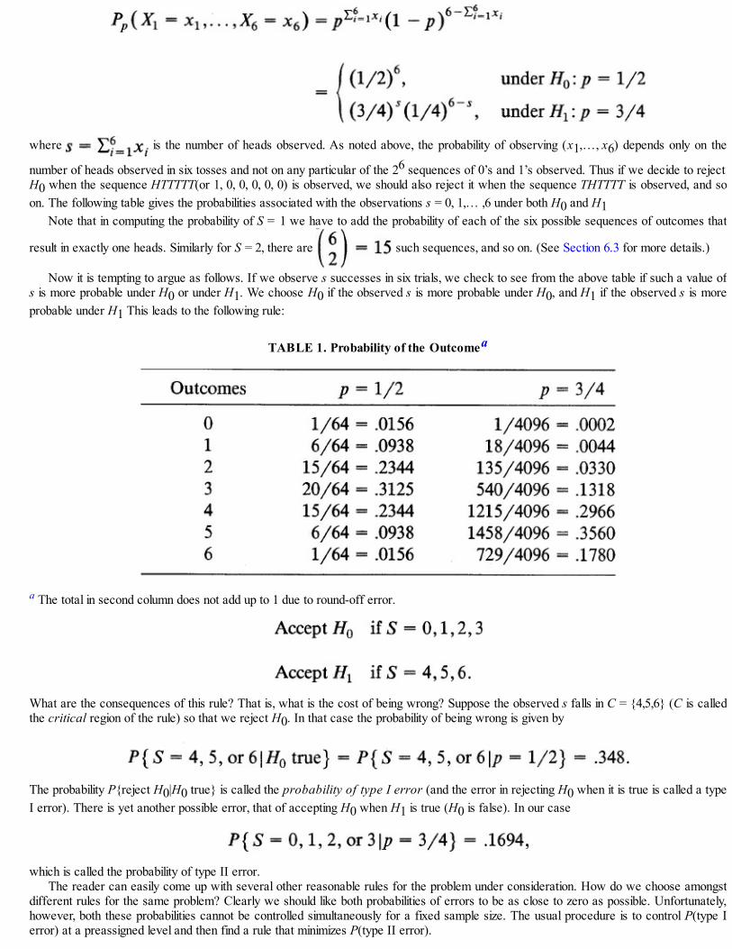
where is the number of heads observed. As noted above, the probability of observing (x1,…, x6) depends only on the

number of heads observed in six tosses and not on any particular of the 26 sequences of 0’s and 1’s observed. Thus if we decide to rejectH0 when the sequence HTTTTT(or 1, 0, 0, 0, 0, 0) is observed, we should also reject it when the sequence THTTTT is observed, and soon. The following table gives the probabilities associated with the observations s = 0, 1,… ,6 under both H0 and H1

Note that in computing the probability of S = 1 we have to add the probability of each of the six possible sequences of outcomes that

result in exactly one heads. Similarly for S = 2, there are such sequences, and so on. (See Section 6.3 for more details.)

Now it is tempting to argue as follows. If we observe s successes in six trials, we check to see from the above table if such a value ofs is more probable under H0 or under H1. We choose H0 if the observed s is more probable under H0, and H1 if the observed s is moreprobable under H1 This leads to the following rule:

TABLE 1. Probability of the Outcomea

a The total in second column does not add up to 1 due to round-off error.

What are the consequences of this rule? That is, what is the cost of being wrong? Suppose the observed s falls in C = {4,5,6} (C is calledthe critical region of the rule) so that we reject H0. In that case the probability of being wrong is given by

The probability P{reject H0|H0 true} is called the probability of type I error (and the error in rejecting H0 when it is true is called a typeI error). There is yet another possible error, that of accepting H0 when H1 is true (H0 is false). In our case

which is called the probability of type II error.The reader can easily come up with several other reasonable rules for the problem under consideration. How do we choose amongst

different rules for the same problem? Clearly we should like both probabilities of errors to be as close to zero as possible. Unfortunately,however, both these probabilities cannot be controlled simultaneously for a fixed sample size. The usual procedure is to control P(type Ierror) at a preassigned level and then find a rule that minimizes P(type II error).

We will see in Chapter 11 that the rule considered above turns out to be the best in a certain sense. See also Examples 4 and 5.

Example 2. MPG Rating of a New Car Model. A new automobile model has just been introduced and the manufacturer claims thatit gives an average of 48 miles per gallon (mpg) in highway driving. A consumer protection agency decides to test this claim. It takes arandom sample of 15 cars. Each car is then run on a stretch of highway and it is found that the sample average mileage per gallon ofgasoline is 42. This figure is less than that claimed by the manufacturer. Is it, however, low enough to doubt the manufacturer’s claim?Could the difference between the claimed average and the observed sample average be due to chance?

Let μ be the true (unknown) average for the model. The correct thing to do is to assume that the manufacturer’s claim is right so thatthe null hypothesis that we wish to put to test is H0: μ = 48 mpg. The alternative hypothesis is H1: μ < 48 mpg. Let Xi represent the mpgof the ith car i = 1, 2,,…, 15, in the test run. We are given that for a sample of size n = 15, the sample average x is 42. If the observedvalue of X were at least 48 there would be no reason to question the validity of H0. Since the observed value of X is 42, it is natural to askthe following question: How probable is it to observe a value of X as small as 42 in random sampling from a population with μ = 48? (Wehave said that X is a good estimate of μ so we expect large values of X under H0 rather than under H1). If this probability is “small” theevidence against H0 is strong, and if the probability is “large” the evidence against H0 is weak.

The problem, therefore, is to compute PH00(X ≤ 42). For an exact computation of this probability, we need to know the distribution ofX. This means that we have to make certain assumptions about the underlying distribution of the Xi’s. If we believe that the family ofpossible densities of Xi is {f(x, μ), μ, > 0} where f is completely specified when μ is specified, then

This last multiple integral can be evaluated to give PH0(X ≤ 42). On the other hand, if n is large it may be possible to approximate PH0

(X≤ 42).

If we are not willing to assume that the family of distributions of Xi is parametric but only that it is continuous and symmetric about μ,then we cannot compute PH0

(X ≤ 42) since we do not know f under H0. According to our assumption, Xi has a density that is symmetricabout the median μ = 48 under H0. Thus, under H0, P(Xi ≥ 48) = P(Xi ≤ 48) = 1/2 so that we expect about half the sample Xi’s to besmaller than 48 and about half larger than 48. If, however, we observe a relatively large number of Xi’s smaller than 48, then we wouldsuspect that the median is smaller than 48. If we know each of the 15 values of Xi we could simply count the number of Xi’s that aresmaller than 48 and base our decision whether to accept or reject H0 on the magnitude of this number. This nonparametric approach leadsto the well known sign test, which will be discussed in detail in Section 6.3.

Example 3. Response Times for Two Stimuli. In order to compare the lengths of response time for two different stimuli in cats, bothstimuli are applied to each of n cats and the response times are recorded in seconds. The object is to determine if there is any differencein mean response times for the two stimuli. Let (X1, Y1),…, (Xn, Yn) be the response times for the n subjects and suppose Di = Xi – Yi.Let us now choose a probabilistic model for the problem. Suppose we are only willing to assume that Di = Xi – Yi, i = 1, 2,…, n is arandom sample from a continuous distribution F ∈ where is the class of all continuous distribution functions on the real line. Then

is a nonparametric family. Let p = P(Xi > Yi).In view of Problem 3.6.16 the null hypothesis of no difference between the stimuli (that is, Xi and Yi are identically distributed)

translates to

and the alternative hypothesis is

If, on the other hand, we are willing to narrow down further by assuming that the common distribution F of the Di’s is given by thedensity

Then is a paramatrics family and H0 translates to

and H1 to

The point is that the procedure we use depends on the assumptions we make concerning . The more we know about the better weshould be able to do. The nonparametric case of this example is discussed in Section 6.3 and the parametric case in Section 8.7.

We are now ready to formalize the notions introduced in the above examples. Let X1, X2,…, Xn be thedata vector (often X1, X,…, Xn will be a random sample) with joint distribution function Fθ, θ ∈ Θ. Let = {Fθ: θ ∈ Θ}.

DEFINITION 1. A statistical hypothesis is an assertion about the joint distribution Fθ of (X1,…, Xn).The statement being tested that Fθ ∈ 0 = {Fθ: θ ∈ Θ0} is called the null hypothesis, and we abbreviateby writing it as H0: θ ∈ Θ0. The rival statement that we suspect is true instead of H0 is called thealternative hypothesis and we abbreviate by writing H0: θ ∈ Θ1 = Θ – Θ0. The hypothesis under test iscalled nonparametric if 0 is a nonparametric family and parametric if 0 is a parametric family.

Usually the null hypothesis is chosen to correspond to the smaller or simpler subset ΘO of Θ and is astatement of “no difference.” In all cases we consider the null hypothesis will be of the form θ = θ0, θ ≥θ0, or θ ≤ θ0. Note that the equality sign always appears in the null hypothesis, whereas the strictinequality sign will always appear in H1. If the distribution of (X1,…,Xn) is completely specified by ahypothesis we call it a simple hypothesis, otherwise the hypothesis is called composite. Thus, wheneverΘO or Θ1 consists of exactly one point the corresponding hypothesis is simple, otherwise it is composite.

Let be the set of all possible values of (X1, X2,…, Xn). Then ⊆ Rn.

DEFINITION 2. (TEST). A rule (decision) that specifies a subset C of such that

is called a test of H0 against H1 and C is called the critical region of the test. A test statistic is a statisticthat is used in the specification of C.

One can make two types of errors.

DEFINITION 3. (TWO TYPES OF ERRORS).

For a simple null hypothesis H0: θ = θ0 against a simple alternative H1: θ = θ1(θ1 > θ0), the two typesof error probabilities are exhibited in Figure 1.

Ideally, we should like both types of error to have probability 0, but this is impossible except intrivial cases. We therefore have to content ourselves by trying to keep these probabilities at an acceptablysmall level. It is customary, however, to fix the probability of type I error at a preassigned (small) levelα, 0 < α < 1, and then try to minimize the probability of type II error.

DEFINITION 4. (SIZE OF A TEST). A test of the null hypothesis H0: θ ∈ Θ0 against H1: θ ∈ Θ1 issaid to have size α, 0 ≤ α ≤ 1, if

The chosen size α is often unattainable. Indeed in many problems only a countable number of levels αin [0, 1] are attainable. In that case we usually take the largest level less than α that is attainable. One alsospeaks of a critical region C of significance level α if

If supθ∈Θ0Pθ(C) = α then the level and the size of C both equal α. On the other hand, if supθ∈Θ0

Pθ(C) < α,then the size of C is smaller than its significance level α. A chosen significance level α is usuallyattainable.

If H0 is a simple hypothesis, then it is clear that PH0(C) is the size of the critical region C, which may

or may not equal a given significance level α.The choice of a specific value for α, however, is completely arbitrary. Indeed it is not strictly a

statistical problem. Considerations such as the possible consequences of rejecting H0 falsely, theeconomic and practical implications of rejecting H0, and so on, should influence the choice of α. Wetherefore follow an alternative approach, wherever possible, by reporting the so-called P-value of theobserved test statistic. This is the smallest level α at which the observed sample statistic is significant.

Figure 1

Before we give a formal definition, let us return to Example 1. Suppose S = 5 is observed. Thenunder H0, P(S = 5) = .0938. The probability of interest, however, is not P(S = 5) but P(S ≥ 5) since theprobability PH0

(S = 6) is even smaller, and if we reject H0 when S = 5 is observed we should do so alsowhen a more extreme value of S is observed. This motivates Definition 5 below.

Suppose the appropriate critical region for testing H0 against H1 is one-sided. That is, suppose that Cis of the form {T ≥ c1} or {T ≤ c2} where T is the test statistic.

DEFINITION 5. (P-VALUE). The probability of observing under H0 a sample outcome at least asextreme as the one observed is called the P-value. If t0 is the observed value of the test statistic and thecritical region is in the right tail then the P-value is PH0

(T ≥ t0). If the critical region is in the left tail thenthe P-value is PH0

(T ≤ t0). The smaller the P-value, the more extreme the outcome and the stronger theevidence against H0.

In most problems considered in this text P-value is a well defined quantity. If the critical region C istwo-sided, that is, if C is of the form (T ≥ t1 or T ≤ t2), then we will double the one-tailed P-value andreport it as the P-value even if the distribution of T is not symmetric. The P-value is variously referred toas the descriptive level or the effective level or the level attained.

Whenever the P-value is well defined, it can be interpreted as the smallest level at which theobserved value of the test statistic is significant. Reporting a P-value conveys much more information thansimply reporting whether or not an observed value of T is statistically significant at level α. Indeed, if thelevel α is preassigned and p0 is the P-value associated with t0, then t0 is significant at level α if P0 ≤ α.Often the statistician does not have much feeling about the economic consequences or the practicalimplications of the decision to be reached. Reporting the P-value permits each individual to choose his orher level of significance.

In many instances we do not have readily available tables of the null distribution (that is, distributionunder H0) of the test statistic. Even in such cases it is desirable to report the interval in which the P-valuelies.

Let us now turn our attention to the probability of a type II error. In order to assess the performance ofa test under the alternative hypothesis, we make the following definition.

DEFINITION 6. (POWER FUNCTION). Let C be the critical region of a test of hypothesis H0 againstH1. Then the function

as a function of θ is called the power function of the test.We note that if θ ∈ Θ0 then β(θ) is the probability of a type I error, and if θ ∈ Θ1 then β(θ) equals 1 –

P (type II error). Thus minimization of a type II error probability is equivalent to the maximization of β(θ)for θ ∈ Θ1 subject to the (significance) level requirements, namely, that

In the case when Θ0 = {Θ0}, H0 is a simple null hypothesis and β(θ) is the size of the test. If Θ1 = {θ1}then

Figure 2 shows some typical power functions.If H1 is composite, the following definition provides an optimality criterion for selecting a test.

DEFINITION 7. (UNIFORMLY MOST POWERFUL TEST). A test with critical region C of the nullhypothesis H0: θ ∈ Θ0 is said to be uniformly most powerful of its size supθ∈Θ0

Pθ(C) if it has themaximum power among all critical regions C’ of significance level supθ∈Θ0

Pθ(C). That is, C is best(uniformly most powerful) if for all tests C′ with PΘ(C′) ≤ supθ∈Θ0

Pθ(C), θ ∈ Θ0 the inequality

holds for each θ ∈ Θ1.

Figure 2. Some typical power functions.

Uniformly most powerful tests do not exist for many hypothesis-testing problems. Even when they doexist, they are often not easy to find. In the rest of this section we consider some examples to illustrate theconcepts that we have introduced. We will restrict ourselves mostly to simple cases when we havesamples of size 1 or 2 in order to avoid distributional problems. In Chapter 11 we study some generalmethods of finding good tests. In this section we will appeal to intuition in finding reasonable testprocedures.

Remark 1. It is important to remember that the P-value is computed under H0 whereas the power is(essentially) computed under H1. An event that has small probability under H0 does not necessarily havelarge probability under H1 That is, an event that is rare under H0 does not have to be relatively frequentunder H1. Thus, in order to properly evaluate the strength of evidence against H0 on the basis of themagnitude of the P-value, we also need to look at the power of the test.

Remark 2. Inferential statements are not probability statements in the sense that once a sample is takenand the decision is made on the basis of this sample then there is no probability attached to the inference.The statement is either true or false and we will never know that unless we know θ. As pointed out in thecase of confidence intervals (see remarks following Definition 4.3.6), all these statements can be given a“long run” interpretation. Thus, “a test has significance level α” does not mean that when the test isapplied to a specific sample and we reject H0, the probability of rejecting H0 falsely is at most α. Inrelative frequency terms it simply means that if the same test is performed on a large number, say N, ofsamples from the same population and if H0 were true then about αN of the samples will result inrejection of H0.

Several examples of nonparametric tests appear in Chapters 6 and 11.

Example 4. Is the Coin Fair? Let us return to Example 1 where we toss a coin six times. Let X1, X2,…, X6 be independent andidentically distributed with common probability function

Then

and H0: p = 1/2 is a simple parametric hypothesis whereas H1: p ≠ 1/2 is a composite hypothesis. We can use Table 1 in Example 1 tocompute the P-values associated with the various values of the test statistic S.

TABLE 2. Power Function of C = {0, 6}

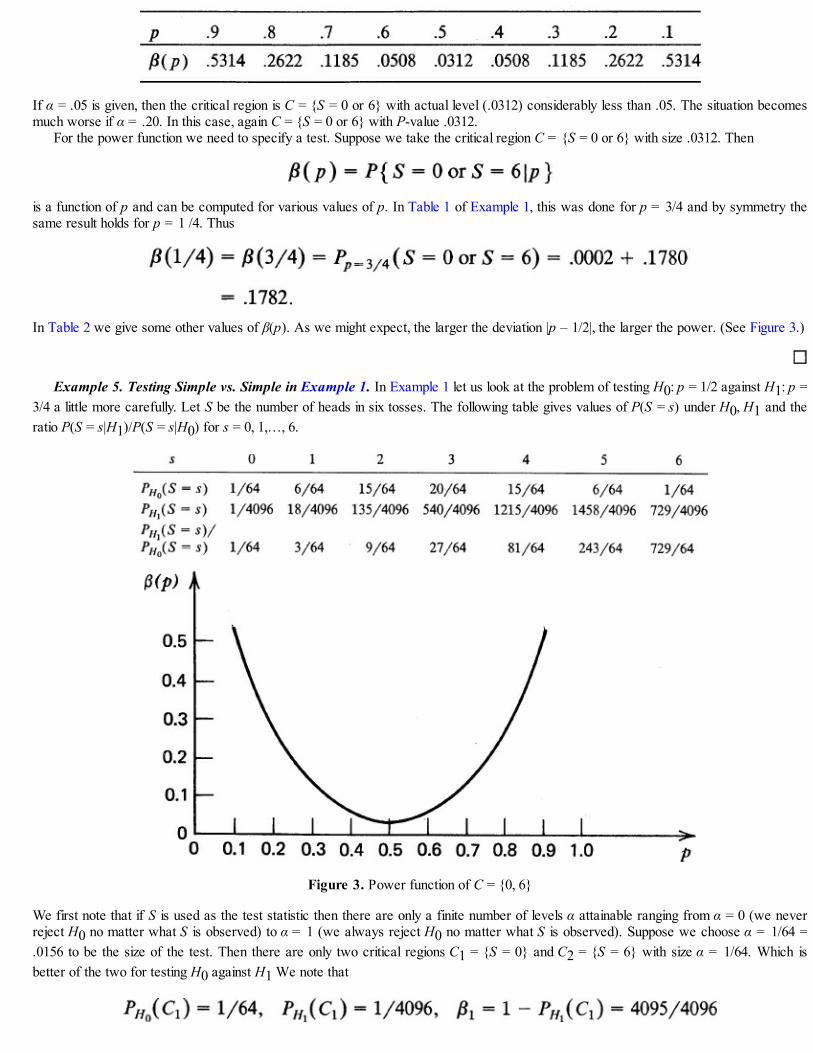
If α = .05 is given, then the critical region is C = {S = 0 or 6} with actual level (.0312) considerably less than .05. The situation becomesmuch worse if α = .20. In this case, again C = {S = 0 or 6} with P-value .0312.

For the power function we need to specify a test. Suppose we take the critical region C = {S = 0 or 6} with size .0312. Then

is a function of p and can be computed for various values of p. In Table 1 of Example 1, this was done for p = 3/4 and by symmetry thesame result holds for p = 1 /4. Thus

In Table 2 we give some other values of β(p). As we might expect, the larger the deviation |p – 1/2|, the larger the power. (See Figure 3.)

Example 5. Testing Simple vs. Simple in Example 1. In Example 1 let us look at the problem of testing H0: p = 1/2 against H1: p =3/4 a little more carefully. Let S be the number of heads in six tosses. The following table gives values of P(S = s) under H0, H1 and theratio P(S = s|H1)/P(S = s|H0) for s = 0, 1,…, 6.

Figure 3. Power function of C = {0, 6}

We first note that if S is used as the test statistic then there are only a finite number of levels α attainable ranging from α = 0 (we neverreject H0 no matter what S is observed) to α = 1 (we always reject H0 no matter what S is observed). Suppose we choose α = 1/64 =.0156 to be the size of the test. Then there are only two critical regions C1 = {S = 0} and C2 = {S = 6} with size α = 1/64. Which isbetter of the two for testing H0 against H1 We note that

and

If we choose C1 over C2 then even though both have the same size we are faced with the prospect of rejecting H0 when H0 is true moreoften than rejecting H0 when it is false (H1 is true). On the other hand, if we choose C2, then the probability of rejecting H0 when it istrue is much smaller than the probability of rejecting H0 when it is false. This is clearly a desirable feature of a critical region. Indeed, C2is the best critical region of size α = 1 /64 since it has larger power. In fact

This result is consistent with our intuition. We expect a larger number of successes under H1 than under H0.The ratio PH1

(S = s)/PH0(S = s) also provides us a tool to determine the best critical region for a given value of size α. For example,

we note that the ratio obtains its maximum value for s = 6 which is in the best critical region C2. The ratio tells us that in relative terms,among all values of s the value s = 6 occurs most frequently under H1 than under H0.

Let us take another example. Suppose we choose α = 7/64. Then the only possible critical regions of size α = 7/64 are

We note that the ratio PH1(S = S)/PH0

(S = s) has two largest values for s = 5 and s = 6 so that C6 should be the best critical region. Thefollowing table shows the power for each critical region.

In terms of power, therefore, we see that C6 is the best critical region and C3 the worst. (There are several other critical regions ofsignificance level α = 7/64: C7 = {S = 0 or 6}, C8 = {S = 0}, C9 = {S = 6}, C10 = {S = 1}, C11 = {S = 5}, and C12 = {always acceptH0}. We leave the reader to check that C7 to C12 also have smaller power than C6.)

Example 6. Time to Failure of an Electric Tube. The time to failure, in thousands of hours, of an electric tube produced at a certainplant has density function given by

The mean life is θ thousand hours. In order to determine if the process is in control, a sample of size n is taken and the tubes are put to atest. Let X1, X2,…, Xn be the n failure times. The process is assumed to be in control if θ ≥ 5 so that the null hypothesis that the processis in control is H0: θ ≥ 5 and the alternative is H1: θ < 5. Both H0 and H1 are composite hypotheses. Let be thesample mean. We have said that X is a reasonable estimate of θ and therefore a reasonable candidate for the test statistic. Now largevalues of X tend to support H0 whereas small values of X tend to support H1. It is therefore reasonable to reject H0 if Xis small, that is, ifX ≤ k for some constant k. The question is, how small should X be before we start doubting H0? In other words, what should be the valueof k? This depends on the amount of error that we are willing to allow in rejecting H0 when in fact it is true.

Let us compute the power function of the critical region C = { X ≤ k }. We have for all θ > 0,

Although it is not difficult to evaluate this multiple integral, we will not do so here. In Chapter 8 we show how to find the distribution of when Xi are independent and identically distributed with density f. Once this is done, it is easy to compute Pθ(X ≤ k) with the

help of a univariate integral. We content ourselves here with the case when n = 2. In that case:

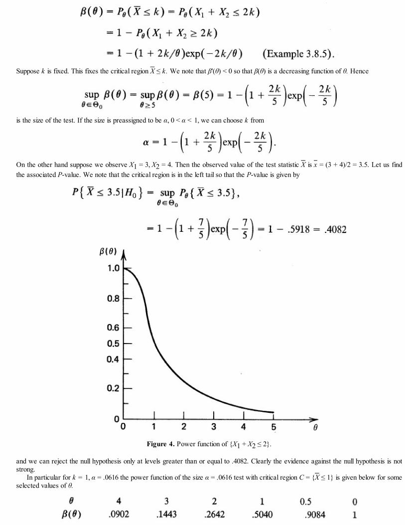
Suppose k is fixed. This fixes the critical region X ≤ k. We note that β′(θ) < 0 so that β(θ) is a decreasing function of θ. Hence

is the size of the test. If the size is preassigned to be α, 0 < α < 1, we can choose k from

On the other hand suppose we observe X1 = 3, X2 = 4. Then the observed value of the test statistic X is x = (3 + 4)/2 = 3.5. Let us findthe associated P-value. We note that the critical region is in the left tail so that the P-value is given by

Figure 4. Power function of {X1 + X2 ≤ 2}.

and we can reject the null hypothesis only at levels greater than or equal to .4082. Clearly the evidence against the null hypothesis is notstrong.

In particular for k = 1, α = .0616 the power function of the size α = .0616 test with critical region C = {X ≤ 1} is given below for someselected values of θ.

Figure 4 shows the graph of β(θ) for 0 ≤ θ ≤ 5.

Example 7. Impurities in a Chemical Product The percentage of impurities per batch in a certain chemical product is a randomvariable X with density function

Here Θ = (0, ∞). Let θ0 ∈ (0, ∞) and suppose we wish to test H0: θ ≤ θ0 against H1: θ > θ0 on the basis of a sample of size n = 2.Consider the critical region C = {(x1, x2): x1x2 ≥ k , x1, x2 ≥ 0} where k (< 1) is a fixed positive constant.

This critical region, as we see in Chapter 11, is the best critical region for testing H0 against H1 and is arrived at by considering theratio fθ1

(x1)fθ2(x2)/(fθ0

(x1)fθ0(x2)), for θ1 > θ0, of the joint density of (X1, X2) under H1 and under H0. The reason for considering this

so-called likelihood ratio is similar to the one given for considering the ratio P(S = s|H1)/P(S = s|H0) in Example 5, but we will not gointo it here.

The test statistic here is X1X2, and both H0 and H1 are composite hypotheses. The size of C is given by:

Figure 5. {(x1, x2): x1x2 ≥ k}

In view of Figure 5 we have

Since k ≤ 1, so that 1 – θ1n k > 0 and kθ is a decreasing function of θ, it follows that β(θ) = Pθ(C) is an increasing function of θ.Hence

gives the size of C with power function

In particular, if θ0 = 1 and k = .8, then the size of C is given by

and the power function for some selected values of θ(> 1) is given below.

Remark 3. The discerning reader will notice that we have used a dual approach in selecting criticalregions: (i) in terms of likelihood, judging whether an observed event has “too small” a probability undera given hypothesis; (ii) in terms of discrepancy from expectations. In some examples (Examples 5 and 7and also Problem 6) and in Remark 1 [under (i)] we have indicated that we need to look at the ratio of thelikelihoods under the two hypotheses. This is done in detail in Sections 11.2 and 11.4. For mostdistributions considered in this book, the two approaches lead to the same conclusion.

Remark 4. It often helps to graph the density or probability function of the test statistic under both H0and H1 (whenever possible) in order to find a reasonable critical region.

Relation Between Hypothesis Testing and Confidence Intervals

There is a close relationship between the confidence interval estimation of a parameter θ and a test ofhypothesis concerning θ, which we now explore. Given a confidence interval at minimum level 1 – α fora parameter θ, we can easily construct a size α test of hypothesis H0: θ = θ0 against one-sided or two-sided alternatives.

PROPOSITION 1. Let [l( ), u( )] be a minimum level 1 – α confidence interval for θ. Then the testwith critical region

is a size α test.

Proof. Indeed,

as asserted.

According to Proposition 1, the 1 – α level confidence interval [l( ), u( )] is the acceptance region ofa size α test of θ = θ0.

If, however, [l( ), u( )] has level at least 1 – α, that is, if

then

and C is a rejection region of θ = θ0 of significance level α.In the converse direction, given the acceptance region of a test of θ = θ0 of size α, we can construct a

minimum level 1 – α confidence interval for θ.

PROPOSITION 2. Let C(θ0) be the rejection region of a size α test of H0: θ = θ0 and let S(θ0)=C(θ0) be the corresponding acceptance region. Then the set of all values of θ ∈ Θ whose acceptanceregions include the observation (x1,…, xn) is a (1 – α) level confidence set for θ. That is, the set

is a (1 – α) level confidence set for θ.

Proof. We have:

so that

for all θ ∈ Θ. It follows that A has confidence level 1 – α.

Example 8. Example 4.3.8 Revisited. In Example 4.3.8 we showed that a (1 – α) level confidence interval for θ based on a singleobservation X from the density function

is given by [X/(1 – α/2), X/(α/2)]. It follows from Proposition 1 that the test with critical region

is a size α test for testing H0: θ = θ0 against H1: θ ≠ θ0. In particular, if α = .05 and X = 1.524 is observed, then a 95 percent confidenceinterval for θ is given by [1.563, 60.96]. Since, for example, θ0 = 1.5 does not belong to this interval, we reject H0: θ = 1.5 at level .05.

Example 9. Confidence Bound for Mean Time to Failure. In Example 6, the time to failure of an electric tube was assumed tohave density function

Suppose we wish to test H0: θ ≥ 5 against H1: θ < 5 on the basis of one observation. Since a large observation tends to support H0, areasonable critical region is given by C = { x ≤ a } for some constant a. If the size of C is to be preassigned at α, 0 < α < 1, then wechoose a to satisfy

so that a = 51n(1 – α)–1. Hence a size α critical region is C = {X ≤ 51n(l – α)–1}.According to Proposition 2 the set

where S(θ) = C(θ) gives a (1 – α) level confidence set for θ. In our case C(θ) = {X ≤ a(θ)} where a = a(θ) is chosen from

Thus

Since

we have:

and

is a (1 – α) level confidence interval for θ. The quantity X/ln(1 – α)–1 is a (1 – α) level upper confidence bound for θ.In particular, if α = .05 and X = 3 is observed than we cannot reject H0: θ ≥ 5 since the critical region of size .05 test is C = {x ≤

51n(1/.95)} = {x ≤ .2565}. We note that the 95 percent level upper confidence bound for θ in this case is 3/ln(1/.95) = 59.49, which isgreater than θ = 5.

Problems for Section 4.4

1. In each case below identify the null and an appropriate alternative hypothesis.(i) The mean age of entering freshman at a certain state university is 18.

(ii) The proportion of blue-collar workers in Detroit is .40.(iii) College graduates earn more money on the average than nongraduates.(iv) American tourists spend more money in Switzerland than do other tourists.(v) Females are more in favor of the Equal Rights Amendment than males.(vi) The median income of college professors is not the same as that of dentists.(vii) Blood storage does not effect triglyceride concentration.(viii) A multiple-choice examination consists of 20 questions. Each question has five possible

answers, only one of which is correct. A student gets 16 correct answers. Is he or she guessingthe answers?

(ix) Two brands of denture cleansers are not equally effective in preventing accumulation of stain ondentures.

(x) Method A of training is superior to Method B.(xi) A given die is loaded.(xii) There are sex differences in brand preference for a particular soft drink.(xiii) The average birth weight of babies in a certain hospital is less than 7.5 pounds.(xiv) There is no sex difference in average birth weight of babies born in a certain hospital.

2. A lady claims that she is able to tell by taste alone whether a cup of tea has been made with tea bagsor with loose tea leaves. In order to test her claim, she is asked to taste eight pairs of cups of tea. Onecup of each pair is made with a tea bag and the other with loose tea leaves of the same type of tea.Suppose she is able to identify correctly in six cases.

(i) State the null and alternative hypotheses.(ii) What is the P-value associated with the observed number of correct identifications?(iii) Find the size of the following critical regions: (X ≥ 5), (X ≥ 6), (X ≥ 7), (X ≥ 8), where X is the

number of correct identifications.

3. It is believed that a typist makes many more errors, on the average, during the afternoon than in themorning. The number of errors, X, per page has approximately the probability function

where X = λ > 0. Suppose further that during the morning session the average number of errors λ isknown to be 1.25. In order to test this belief a random sample of eight pages (known to have beentyped either in a morning or in an afternoon session) was checked and found to contain a total of 19errors.

(i) State the null and alternative hypotheses.(ii) Find a test of H0 against H1 that has significance level α = .10.(iii) Find the P-value associated with the observed number of errors in eight pages. Would you reject

H0 at level α = .01?[Hint: Use the result that S8 = X1 + X2 + ··· + X8 has the distribution P(S8 = s) = e–8λ(8λ)s/s!, s =0, 1, 2,…. Table A4 in the Appendix gives the cumulative probabilities for Ss.]

4. According to a genetic theory, about 40 percent of a certain species have a particular characteristic. Inorder to test the theory a random sample of seven is taken and it is found that only one individual in

the sample has the characteristic.(i) What are the null and alternative hypotheses?(ii) What is a reasonable test statistic?(iii) What is the P-value associated with the outcome?

5. Let X be a single observation from probability function

Consider the test with critical region C = { X ≥ 4} for testing H0: λ = 1 against H1: λ = 2. Find thesize of the test, the probability of type II error, and the power of the test.

6. In Problem 5 suppose a sample of size 2 is taken to test H0: λ = 1 against H1: λ = 2. Consider thecritical region

Find the size and the power of this critical region.[Hint: Simplify and show that the critical region C can be written as {(x1, x2): x1 + x2 ≥ 4}.]

7. A random sample of two observations is taken from the distribution with density function

The null hypothesis H0: θ = 2 is rejected against the alternative H1 : θ < 2 if the observed values x1,x2 of X1, X2 fall in the set. {(x1, x2): x1 + x2 < 1.5, x1 ≥ 0, x2 ≥ 0}. Find the size of the test and itspower function at θ = 1.8, 1.6,…,.2.

8. In Problem 7 suppose we wish to test H0: θ = 2 against H1: θ = 1. Consider the critical region

where f(x, θ) = (1/θ)exp(–x/θ) for x ≥ 0 and zero

elsewhere. Find the size of this critical region and the power at θ = 1.

9. A random variable X has probability function

A sample of size one is taken. If x ∈ {3, 4}, we reject H0 and accept it otherwise.(i) Find the probability of type I error.(ii) Find the power of the test and the probability of type II error.

10. In Problem 2 suppose the lady does have certain ability to distinguish between the two methods ofmaking tea. In particular, suppose that the probability that she is able to correctly identify the methodis p = 2/3.(i) Find the probability of type II error and the power of each of the four critical regions.(ii) Given α = .0352, find the best critical region of size α.

11. A gambler believes that a certain die is loaded in favor of the face value 6. In order to test his belief,he rolls the die five times. Let X be the number of times a six shows up in five rolls and consider therejection regions Ci = {X ≥ i}, i = 0, 1, 2,…, 5.(i) State the null and alternative hypotheses.(ii) Find the size of each of the six critical regions.(iii) Find the power of each of the six critical regions at p = P(6) = 1/5.

12. In Problem 11 suppose Y is the number of rolls needed to get the first 6. Consider the critical regionsDi = {Y ≤ i}, i = 1, 2,… based on the test statistic Y.(i) Find the size of each Di, i ≥ 1.(ii) Find the power of each critical region when p = P(6) = 1/5.(iii) Suppose in two experiments the average number of rolls needed to get a 6 was 4.5. Find the

associated P-value. Would you accept H0 at 10 percent level of significance?

13. The life length of a fuse has density function

Find a size α test of H0: θ = θ0 against H1: θ ≠ θ0 of the form C= {x: x < c1 or x > c2}, where c1 < c2.(Choose c1, c2 such that each tail has probability α/2.) What is the power function of your test? Find a1 – α level confidence interval for θ.

14. Let X have density function

Find a size α test of H0: θ ≤ θ0 against H1: θ > θ0 based on one observation. Find a 1 – α level lowerconfidence bound for θ. (Hint: Graph f under H0 and H1.)

15. Let X have density function

Find a size α test of H0: θ = 1 against H1: θ ≠ 1 based on a single observation. Find the powerfunction of your test. (Hint: Graph f under H0 and H1.)16. Let X have density function

Find a size α test of H0: θ ≥ θ0 against H1 : θ < θ0 based on one observation. Find the power functionof your test. Find a 1 – α level upper confidence bound for θ. (Hint: Graph f under H0 and H1)

17. The content X of a metal in any alloy has density function given by f(x) = 2x/θ2, 0 ≤ x ≤ θ, and zeroelsewhere. It is required that H0: θ = 4 be tested against H1: θ > 4. A sample of size one produced theobservation x = 3.

(i) What is the P-value associated with the sample? What is the P-value if x = 3.5 is observed?(ii) Find a size α test of H0 against H1.(iii) Find the power function of your size α test.(iv) Find a minimum level 1 – α lower confidence bound for θ.

[Hint: For part (ii), graph f under H0 and H1.]

18. (i) For the following densities, find a size α(> 1/2) test of H0: θ = θO against H1: θ > θ0 based on asample of size 1.(a)

(b) f(x) = 2(θ – x)/θ2, 0 < x < θ, and zero otherwise.(c) f(x) = |x|/θ2, 0 ≤ |x| < θ, and zero elsewhere.(d) f(x) = (θ – |x|)/θ2, 0 ≤ |x| < θ, and zero elsewhere.

(ii) Find the power function of each test in part (i) for θ > θ0.(iii) Find the minimum level 1 – α lower confidence bound for θ in each case of part (i) from your

size α test.

4.5 FITTING THE UNDERLYING DISTRIBUTION

Most of the work we have done so far assumes that we know the probability distribution of the randomvariables of interest except perhaps for the numerical value of some parameter or parameters. This meansthat we specify a parametric model for the observable phenomenon. If the conditions describing theexperiment are precise enough to suggest that the distribution can be closely approximated by a knowndistribution F = Fθ (except perhaps for θ), then the problem is simply to estimate θ from the data and thenuse a test to check if there is agreement between the mathematical model and the data. Often, however,one has little or no prior information on F. This may be because the conditions describing the physicalexperiment are too vague or incomplete to suggest any particular model. In that case we can try toestimate either the distribution function or the density function.

Before making a specification of F, it is a good practice to look at the data in a graphical from inorder to see if they could have come from one of a known family of distributions. A list of some wellknown distributions and their properties is useful for this purpose. This is provided in Chapters 6 and 7.

One of the simplest ways of looking at the data is to make a stem-and-leaf plot. It is best introduced

with the help of an example.

Example 1. Weights of Students in a Statistics Class . A sample of 39 students was taken from a large class in an elementarystatistics course at a state university and their weights (in pounds) were recorded as follows:

Each weight, regarded as a three-digit number, is arranged in a display by designating the first two digits (the hundredth-place and thetenth-place digits) as the stem and the remaining digit as the leaf. The distinct stem values are then listed vertically and the leaves arerecorded on the lines corresponding to their stem values. Thus, the weight 96 has a stem value of 9 and leaf value of 6, which is recordedon the horizontal line corresponding the stem value 9, and so on. Figure 1 gives a stem-and-leaf plot of the data on weights.

Figure 1. Steam-and-Leaf plot for weights of students (in pounds).

A stem and leaf plot for the data on weight in Example 1 contains all the information on weights ofstudents in the sample. It is quick, simple, easy to draw and quite effective. No hand drawing is required.The shape of the plot suggests the form of the underlying density function. (One can imagine or even drawa curve through the leaves appearing on the extreme right of each stem value.)

The classical method of presenting data is to construct a histogram. We first encountered a histogramin Section 3.3 where we drew histograms of probability functions of integer valued random variables byerecting bars or rectangles on intervals (x – 1/2, x + 1/2) of unit length with midpoints x, where x is aninteger. The height of the rectangle on base (x – 1/2, x + 1/2) was taken to be proportional to P(X = x).

In order to draw a histogram for a set of continuous measurements, the range (largest observation-smallest observation) is partitioned into intervals of preferably equal length. When the observations areunbounded (the range is infinite) we take unbounded intervals on one or both extremes as required. Thenumber of observations in each interval is called the frequency of the interval, or class frequency.Rectangles are then drawn with class intervals as base and height proportional to the class frequency sothat the area of a rectangle on a class interval is proportional to the frequency of that class interval. Astem-and-leaf plot is in effect a histogram for class intervals of length equal to the difference between twoconsecutive stem values. The frequency of each class interval is simply the length of the row for the

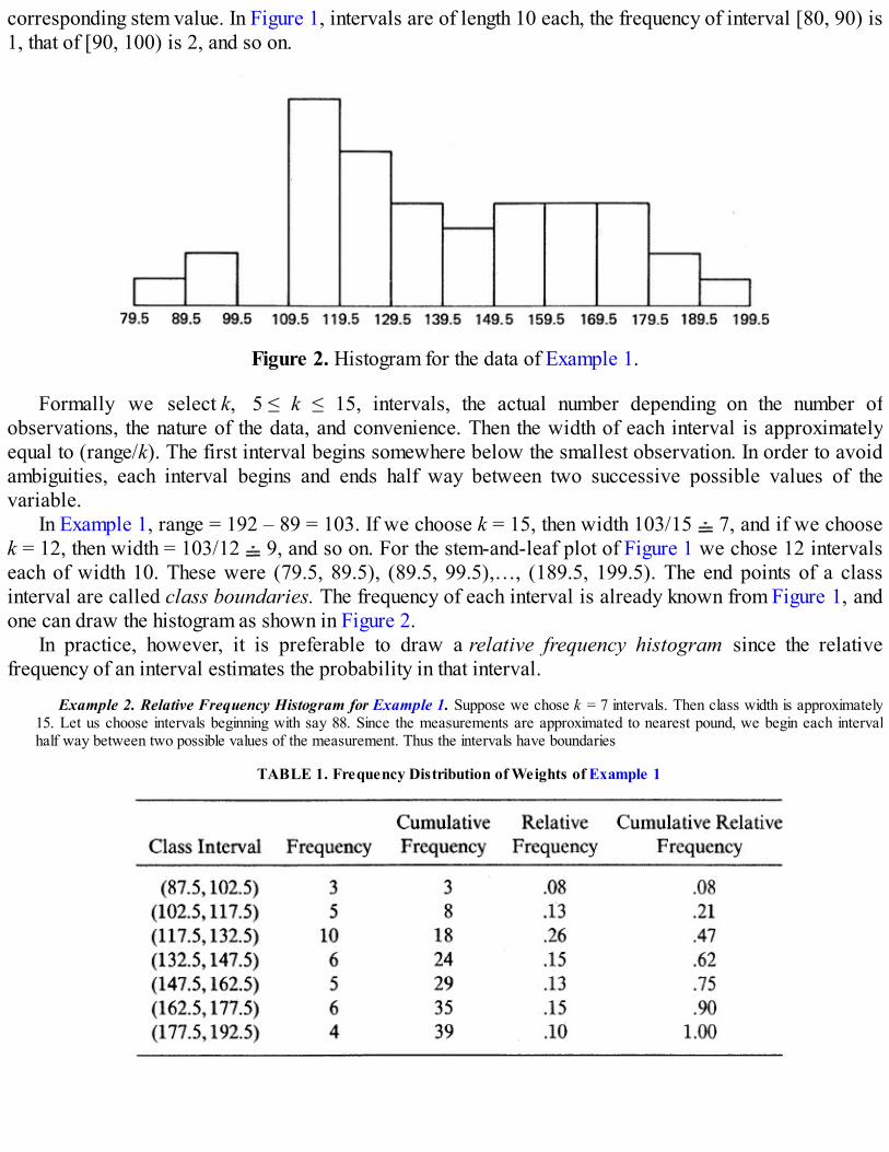
corresponding stem value. In Figure 1, intervals are of length 10 each, the frequency of interval [80, 90) is1, that of [90, 100) is 2, and so on.

Figure 2. Histogram for the data of Example 1.

Formally we select k, 5 ≤ k ≤ 15, intervals, the actual number depending on the number ofobservations, the nature of the data, and convenience. Then the width of each interval is approximatelyequal to (range/k). The first interval begins somewhere below the smallest observation. In order to avoidambiguities, each interval begins and ends half way between two successive possible values of thevariable.

In Example 1, range = 192 – 89 = 103. If we choose k = 15, then width 103/15 7, and if we choosek = 12, then width = 103/12 9, and so on. For the stem-and-leaf plot of Figure 1 we chose 12 intervalseach of width 10. These were (79.5, 89.5), (89.5, 99.5),…, (189.5, 199.5). The end points of a classinterval are called class boundaries. The frequency of each interval is already known from Figure 1, andone can draw the histogram as shown in Figure 2.

In practice, however, it is preferable to draw a relative frequency histogram since the relativefrequency of an interval estimates the probability in that interval.

Example 2. Relative Frequency Histogram for Example 1. Suppose we chose k = 7 intervals. Then class width is approximately15. Let us choose intervals beginning with say 88. Since the measurements are approximated to nearest pound, we begin each intervalhalf way between two possible values of the measurement. Thus the intervals have boundaries

TABLE 1. Frequency Distribution of Weights of Example 1

Figure 3. Relative frequency histogram for Table 1.

Table 1 gives the relevant information.The relative frequency histogram is given in Figure 3.

Remark 1. It is clear that there is a certain amount of arbitrariness involved in the construction of ahistogram. Nevertheless, unless one selects the number of intervals (and hence size of intervals) ratherpoorly, a histogram gives a rough idea of the shape of the underlying distribution.

Remark 2. It is not necessary, although it is often desirable, to choose equal length intervals. If onechooses intervals of different lengths, one can still draw a histogram for the data. The point to rememberis that it is the area of the rectangle that represents (or is proportional to) the frequency or relativefrequency of the interval and not the height of the rectangle.

Remark 3. When X is of the discrete type, it is easy to construct a frequency distribution for the data.All we need to do is to count the frequency of each of the possible values of X.

Let us now turn our attention to the theory underlying the histogram estimation of a density function. Inthe discrete case, the relative frequency of {X = xj} estimates P(X = xj) , j = 1, 2,…. In the continuouscase, let the range be partitioned into k class intervals Ij, j = 1, 2,…, k and suppose that Ij = (aj–1, aj), j =1, 2,…, k where a0 < a1 < … < ak. Define the function by

where fj is the frequency of the class interval Ij and is the total number of observations. Thefunction defined on (– ∞, ∞) is called a relative frequency histogram. We note that

Hence defines a density function and is used as an estimate of the underlying density function f. Inparticular, an estimate of the probability of an event A is given by

If, for example, A = ∪jIj then

We will see that (A) is an unbiased and consistent estimate of P(A) (see Problem 5.4.6 and alsoProblem 5.6.11).

Yet another way to look at the data is to draw the sample or empirical distribution function. Supposewe observe the sample X1 = x1, X2 = x2,…, Xn = xn. Then we can construct a distribution function from x1,x2,…, xn by assigning to each xi a probability mass of 1/n. This leads to the following definition.

DEFINITION 1. (SAMPLE OR EMPIRICAL DISTRIBUTION FUNCTION).Let x1, x2,…, xn be the observed values of the random sample X1, X2,…, Xn from some distribution

function F. Then the function

defined for each x ∈ is called the empirical distribution function.

We first note that 0 ≤ n(x) ≤ 1 for all x, and, moreover, that n is right continuous andnondecreasing. Clearly, n(– ∞) = 0 and n(∞) = 1. It follows that n is a distribution function.Moreover, n is a discrete type distribution function even though F may be continuous. We will see(Examples 5.4.3 and 10.3.8) that n is a consistent and unbiased estimate of F. Note that n(x) is therelative frequency of the event { X ≤ x}.

Example 3. Empirical Distribution Function for Weights of Students (Example 1). Let Xi be theweight of the ith student. Then the 39 weights of Example 1 are the 39 observations x1, x2,…, x39. Clearly,

39(x) = 0 for x < 89, 39(89) = 1/39, 39(92) = 2/39, 39(96) = 3/39,… 39(192) = 1, and 39(x) = 1for x > 192. Figure 4 shows the graph of 39(X).

Figure 4. Empirical distribution function for distribution of weights.

Unless n is large, n looks a bit silly as an estimate of F when F is continuous since n goes up byjumps of sized 1/n whereas F increases continuously. But when n is large, n is tedious to draw since itamounts to listing all the n observations in an increasing order of magnitude. Moreover, the step size 1/nis small when n is large. For large n it is usual to group the observations in a frequency distribution.How, then, do we use n to compute an estimate of F from a grouped frequency distribution? Suppose theintervals are Ij = (aj–1, aj), j = 1, 2,…, k. Then

Let us graph the points and join the successive points by line segments. The resulting plot is known as an

ogive and provides an estimate of F from a ground frequency distribution.Let denote the ogive function. Then 0 ≤ (x) ≤ 1 for all x ∈ ,

and is right continuous and nondecreasing on . Since (– ∞) = 0 and (∞) = 1, is a distributionfunction.

We note that the slope of the line joining the points (aj–1, n(aj–1)) and (aj, n(aj)) is given by

for x ∈ (aj–1, aj]. It follows that ′(x) = (x) for x ∈ (aj–1, aj).For the frequency distribution of Table 1, Figure 5 shows the plot of the ogive.

Figure 5. Ogive function for Table 1.

So far we have answered the following questions: What does the underlying density function f or thedistribution function F look like? How do we estimate f or F? The next question that one needs to answeris: Does f or F look like a known or specified distribution? One obvious way to proceed is to plot thespecified f (or F) and its estimate (or n or ) on the same paper and see how good the agreement is.If the agreement between and f is good, it is reasonable to conclude that f is the underlying density.Since the eye can be deceptive, we will have to devise a more scientific procedure to check the fit. Thisis done in Section 9.9 and Chapter 11. Nevertheless, this is a good first step to follow.

Example 4. Random Sampling from the Interval (0, 1). A random sample of 80 points is picked from the interval (0, 1) so that theunderlying density is f(x) = 1, 0 < x < 1, and zero elsewhere. The data are as follows.

Let us construct a relative frequency histogram using 10 equal classes with a0 = .005 and a10 = 1.005. We expect each interval tocontain eight observations. Table 2 gives the relative frequency histogram.

In Figure 6 we plot the histogram estimate of f and f, and in Figure 7 we plot the ogive function estimate of F(the distribution

function corresponding to f) and F. It is not at all clear from these figures whether the agreement between and f or and F should beconsidered good or not. We will have to apply some test of goodness of fit. This is done in Section 9.9.

TABLE 2. Relative Frequency Histogram and Ogive

a This column only gives the values of at upper class boundaries.b Total does not add to 1 owing to round-off error.

Figure 6. Histogram estimate of f, and f.

Finally, we note that the relative frequency histogram can be used to estimate moments of theunderlying distribution and the ogive function can be properly used to estimate the quantiles of F. Forexample, the mean of (x) by definition is given by

where xj = (aj–1 + aj)/2 is called the class mark or the midpoint of class interval Ij. Similarly, thevariance of can be used to estimate var(X). However, the estimate for variance that is frequently used isgiven by

From the ogive function one can estimate the quantile of order p, 0 < p < 1 by simply reading off fromthe graph of the abscissa of the point of intersection of y = p and y = (x).

Problems for Section 4.5

1. The failure times of 50 transistor batteries of a certain kind in hours are as follows:

(i) Construct a frequency distribution using 11 intervals of equal length beginning with 12.55.(ii) Draw the relative frequency histogram and the ogive for the data.(iii) Find an estimate for the mean and the median of the underlying distribution of failure times.

2. The high-school grade point averages of a random sample of 60 entering freshmen are given below.

Construct a relative frequency histogram and an ogive for the data.

3. A die was tossed 120 times with the following results.

How will you estimate the probability function P(X = x), x = 1, 2,…,6 of X, the face value that showsup on a toss? Do the data indicate that the die is fair? [Compare your estimate of P(X = x) and P(X =x) = 1/6, x = 1, 2,…,6 by means of a graph.]

4. For the following data, compute the empirical distribution function and plot it.

What is your estimate of P(X ≤ 3)? Estimate P(X > 4).

5. An urn contains five slips numbered 1 through 5; A random sample of size 18 is taken withreplacement with the following results:

Compute and plot the empirical distribution function. Plot also the underlying distribution function onthe same paper. Estimate

6. A random sample of 60 infants yielded the following heights (in inches):

(i) Construct an appropriate frequency distribution with eight classes of equal length.(ii) Construct the relative frequency histogram and the ogive.(iii) Find estimates of the mean and the median heights of infants.

7. The following random sample of 100 observations is taken from the interval (0, 1):

(i) Construct a frequency distribution with 10 class intervals of equal length.(ii) Construct the relative frequency histogram and the ogive.(iii) Estimate the mean and the quantiles of order p = .25, .5, and .75.

(iv) What is your guess of f and F?

4.6 REVIEW PROBLEMS

1. The breaking strength (in ounces) of a random sample of 50 threads is given below:

(i) Construct a frequency distribution with 5 intervals beginning with 13.95 ounces.(ii) Obtain the histogram estimate of the density function of breaking strength and also the ogive

estimate of the distribution function.(iii) Estimate the mean breaking strength of the population of threads from which the sample was

taken. (There are two ways to do so, either by using the sample observations or by using thefrequency distribution.)

2. Suppose that a student’s score X on a certain examination has density function

(i) Find an unbiased estimate of θ based on a single observation. Find the variance of your estimate.(ii) Consider also the estimate = X. Find the bias and mean square error of .(iii) Find the efficiency of your unbiased estimate relative to .

3. The time X (in hours) between arrivals of customers in a bank is a random variable with densityfunction

(i) Show that the critical region { x: fH0(x) = 0} is the best size 0 critical region for testing H0: θ =

θ0 against H1: θ = θ1 (θ0 > θ1) based on a sample of size 1.(ii) Find the best critical region of size zero for testing H0 against H1 [of part (i)] based on a sample

of size 2.

4. Let X1, X2,…, Xn be a random sample from a distribution function F. Let c be a given constant. Howwill you estimate PF(X1 > c) without the knowledge of F?

In particular, in Problem 1, what is your estimate of the proportion of thread that has breakingstrength greater than 28 ounces?

5. An urn contains N identical slips numbered 1 through N. A random sample of two slips is taken withreplacement in order to estimate N by a confidence interval of level at least 1 – α. Find an equal tailsconfidence interval based on max(X1, X2) where X1 and X2 are the numbers on the first and the second

slip drawn. Hence find a test of H0: N = N0 against H1: N ≠ N0 of significance level α. [Hint: max(X1,X2) ≤ k if and only if X1 ≤ k and X2 ≤ k.]

In particular, if x1 = 8, x2 = 27, and α = .10, what is your interval estimate of N?

6. Let X have density

(i) Find a size α (< 1/2) test of H0: θ = θ0 against H1: θ < θ0 based on a sample of size 1.(ii) Find the power function of your test.(iii) Find an upper confidence bound at minimum level 1 – α for θ.

7. Let X have density

(i) Find a size α test of H0: θ = θ0 against H1: θ < θ0 based on a single observation.(ii) Find the power function of your test.(iii) Find an upper minimum level 1 – α confidence bound for θ.

8. A chemist has taken a sample of size 2 from a chemical compound and tests each sample forproportion of impurity. On the basis of this analysis she would like to determine if the compoundcame from Supplier A or Supplier B. It is known that the proportion of impurity is a random variablehaving density fA(x) = 2x, 0 ≤ x ≤ 1 and zero otherwise if the compound comes from Supplier A anddensity fB(x) = 3x2, 0 < x < 1 and zero otherwise if it comes from Supplier B. Let x1, x2 be the sampleproportions of impurities. The chemist chooses to reject H0 that X has density fA if

Find the size of her test and its power.

9. Two observations were taken from the uniform density

in order to test the null hypothesis θ = θ0 against H1: θ ≠ θ0.(i) Let X be the test statistic.

(a) Find a size α test of H0.

(b) Find the power of your test.(c) Find the minimum level 1 – α equal tails confidence interval for θ.

(ii) Take T(X1, X2) = max(X1, X2) as the test statistic.(a) Find a size α test of H0.(b) Find the power of your test.(c) Find the minimum level 1 – α equal tails confidence interval for θ.

(iii) Compare the powers of your tests in (i) and (ii). (You may assume that α < 1/2.)

10. After the April 20, 1980, helicopter attempt to rescue American hostages held in Iran, it was claimedthat the eight helicopters used in the rescue mission had each flown 20 missions without amalfunction. On the day of the rescue mission, however, three of the eight helicopters involved in therescue failed. Let p = P (failure on a single flight). The assertion that no failures occurred in previousmissions should not be taken to mean that p = 0 but only that p is very small, say p = 1/25. Test H0: p= 1/25 against H1: p > 1/25 to see if there is any inconsistency between the observed failure rate andthe asserted failure rate.

Do the same problem with H0: p = .1 and with H0: p = .01. (You may assume that the failure of anyhelicopter on a mission is independent of the failure of any other helicopter on the mission.)

11. From Table A1 in the Appendix, the following sample of 105 random digits is taken:

(i) Find the histogram estimate of the distribution of digits 0, 1,…, 9.(ii) Compute the empirical distribution function. Graph the empirical distribution function along with

the theoretical distribution function.

† See Remark 2 below for an explanation of the notation F.

CHAPTER 5

More on Mathematical Expectation

5.1 INTRODUCTION

In Chapter 4 we saw that in order to compute the numerical value of a confidence interval or to computethe critical region of a level a test we often need to evaluate a multiple integral. This integration can bereduced to a univariate integral provided we know the distribution of the statistic T(X1 X2…,Xn). Thiswill be done in Chapter 8. When the parameter of interest is μ we often took T(X1 X2,…,Xn) = as anestimate or a test statistic. How do we evaluate the performance of as an estimate for μ without theknowledge of the distribution of ? How do we construct a confidence interval for μ based on withoutthe knowledge of the distribution of ? For this purpose we first need to define the expected value ofT(X1, X2,…,Xn) with respect to the joint distribution of (X1 X2,…,Xn). This is done in Section 5.2. InSection 5.3 we show how to compute T and var(T) when T is a linear function of X1 X2,…,Xn. Thisallows us to compute T and var(T) from the knowledge of Xj, var(Xj), and cov(Xi, Xj). We do not needto know the joint distribution of X1 X2…,Xn. In Section 5.4 we give a precise formulation of the wellknown law of averages and prove a weak version of this result. This so-called weak law of largenumbers allows us to conclude, for example, that , consistent estimate for μ so that for large n, islikely to be near μ. In Section 5.5 we define expected values with respect to a conditional distribution.Suppose X, Y are jointly distributed dependent random variables. How do we predict Y given X = x?More precisely, for what function Φ does the estimate Φ(x) of Y have minimum mean square error (Y –Φ(x))2? The answer, as we show in Section 5.5, is that Φ(x) is the mean of the condition distribution of Ygiven X = x.

5.2 MOMENTS IN THE MULTIVARIATE CASE

Let X be the length and Y the width of a rectangle and suppose that X and Y are random variables. What isthe average area of the rectangle so formed? If X is the total time that a customer spends in a bank and Ythe time spent waiting in line, what is the average service time of the customer at this bank? To answerthese questions we need to define expected value of a real valued function of a random vector.

Let (X1 X2,…,Xk) be a random vector with known joint probability (or density) function. Let g(x1,…,xk) be a real valued function defined on and assume that g itself is a random variable.

DEFINITION 1. If (X1 X2,…,Xk) is of the discrete type and then we define the expected value

(mathematical expectation) of g by:

If, on the other hand, (X1…Xk) has joint density function f and

then we define the expected value of g by:

Some immediate consequences of Definition 1 are listed below. The reader is asked to supply theproofs. (In the following, whenever we write (X1,…,Xk) for any function g we assume that g is arandom variable and the expected value exists in the sense of Definition 1.)

I. Let a and b be constants. Then

II. Let g1 g2,…,gn be real valued functions of X1,…,Xk. Then

III. Let X1 X2…,Xk be independent random variables and g1 g2,…,gk be real valued functions of X1X1…,Xk respectively. Then

Since III is an important result we give a proof. We restrict attention to the continuous case. The prooffor the discrete case (or mixed case) is similar. We have

where fj is the marginal density of Xj and we have used the independence of X1…,Xk. It follows that

as asserted. We emphasize that the converse of property III is not true.Choosing

we see that (in the continuous case):

which is the nth central moment of the marginal distribution of Xj. Thus Xj is the mean and is the variance of the marginal distribution of Xj. In other words, we can compute

moments of each Xj either from the marginal distribution of Xj or from the joint distribution of X1…,Xkwhichever happens to be convenient.

Remark 1. Since Y = g(X1 X2…,Xk) is a (one-dimensional) random variable, it has a distribution thatcan be computed from the joint distribution of X1 X2…,Xk. This is done in Chapter 8. Suppose fY is thedensity function of Y if Y is of the continuous type [or P(Y = yj) is the probability function of Y if it is ofthe discrete type]. If then

Does Y coincide with g(X1 X2…,Xk) as computed in Definition 1? This is true but we will not prove it

here. The point is that if the joint distribution of X1…,Xk is known then we can compute g(X1 X2…,Xk)directly from Definition 1 without computing the distribution of Y = g(X1 X2…,Xk).

Example 1. Mean Service Time at a Bank. Let X be the total time (minutes) that a customer spendsat a bank, and Y the time she spends waiting in line before reaching the teller. Assuming that the customergets into a line immediately after entering the bank, the service time is X — Y and the mean service time isgiven by (X – Y). We can use either Definition 1 or property II with g1(X, Y) = X and g2(X, Y) = Y tocompute (X – Y).

Suppose X, Y have joint density

Then, from Definition 1:

on integration by parts. Alternatively, the marginal of X is given by

and that of Y by

Hence

Example 2. Average Amount of Money Spent on a Commodity. The wholesale price X of a certaincommodity and the total sales Y have a joint distribution given (approximately) by

What is the average amount of money spent on this commodity?Since the total amount of money spent is XY, the average amount of money spent is

Example 3. Families with Three Children. Consider families with three children. Let X denote thenumber of boys and Y the excess of boys over girls. Then X and Y have joint probability function given by

We note that

A look at the table shows that X and Y increase or decrease together and, moreover, that all nonzerovalues are along the diagonal. This suggests that X and Y have a linear relationship. Indeed, Y = (numberof boys less number of girls) = X – (3 – X) = 2X – 3. The measurement of the extent to which X and Y varytogether is the subject of discussion below

Covariance and Correlation

Let X and Y be two random variables with joint distribution function F and marginal distribution functionsF1 and F2 respectively. We recall that X and Y are independent if and only if

for all x, y ∈ . We saw that (stochastic) independence of X and Y simply means that the knowledge ofone of X or Y provides no new probabilistic information about the other variable. Therefore, if X and Yare dependent we feel that X and Y somehow vary together and the knowledge of one variable may allowus to say something about the other. If X is the shoe size and Y the height of an individual and if we knowthat X is large, we feel pretty confident that Y is also large. Similarly, when the price of a commodity goes

up we expect that the demand will go down. If a person has a few drinks we do not hesitate to recommendthat she or he drive carefully or not drive at all, because we feel that the greater the amount of alcohol inthe blood the poorer the motor coordination.

How do we measure this connection or association between X and Y? How do X and Y vary jointly?Any such measure should clearly depend on the joint distribution of X and Y. Moreover, if X and Yincrease together then (X – X)(Y – Y) should be positive whereas if X decreases while Y increases(and conversely) then the product should be negative. Hence the average value of (X – X)(Y – Y)provides a measure of association or joint variation of X and Y.

DEFINITION 2. (COVARIANCE). If (X – X)(Y – Y) exists, we call it the covariance between Xand Y.

If covariance exists, we write:

where μ1 = X and μ2 = Y. Note that

and

For computational purposes, the following formula is sometimes useful:

For the proof of (2), we note that

in view of property II.

PROPOSITION 1. If X and Y are independent,

Proof. If X and Y are independent, it follows from property III that

and the result follows from (2)

Remark 2. The converse of Proposition 1 is false. If cov(X, Y) = 0, it does not follow that X and Y areindependent. For, let X be symmetric ith. X = 0 and . Let Y = X2. Then

but X and Y are strongly dependent. For some exceptions, see Problem 12 and Section 7.7.

Example 4. Covariance Between Service Time and Total Time Spent . For the random variables Xand Y of Example 1, we have

Since and we have from (2)

which is not surprising, since the greater the service time Y the greater the total time spent X

Example 5. Covariance Between Stock and Sales. The weight X in tons of a bulk item stocked by asupplier at the beginning of every month and the weight Y of this item sold by the supplier during themonth have a joint probability density function given by

In order to compute cov(X, Y), we compute:

Hence:

The following result will be quite useful.

PROPOSITION 2. (CAUCHY-SCHWARZ INEQUALITY). I f then σXYexists and

Equality in (4) holds if and only if there exist not both zero such that

Proof Since we have

I f X is degenerate σX = 0 and (4) holds trivially. Hence we may assume that . Choose in (5). Then

and in particular with β = 1,

which is (4). Equality holds in (4) if and only if there exist α and β ∈ (not both zero) such that

That is, if and only if

for some α, β, not both zero, and c ∈ .

Remark 3. In Proposition 2, is a sufficient but not a necessary conditionfor the existence of cov(X, Y). For example, if X and Y are independent then

exists (and equals 0) provided and . In fact cov(X, Y) may exist but X2 or Y2

may be infinite even when X and Y are dependent Problems 14 and 15).

The following result points out an unsatisfactory feature of covariance as a measure of the jointvariation of X and Y.

PROPOSITION 3. Let a, b, c, and d be real numbers. Then

Proof. By definition

COROLLARY 1. Var(aX + b) = a2 var(X).

COROLLARY 2. Let . Then

Proof. Choose in (6)

The covariance between X and Y is positive if X and Y tend to increase or decrease together andnegative if X and Y tend to move in opposite directions. Unfortunately, the covariance is sensitive to thescales of measurement used (Proposition 3). Therefore, it is not possible to interpret what a numericalvalue of cov(X, Y) means. For example, suppose X and Y are measured in meters and cov(X, Y) = 0.001. Ifwe change the scale to centimeters by writing U = 100X and V = 100 Y, then from (6):

A simple change in units of measurement leads to a completely different impression about the strength ofrelationship between X and Y. It is clear, therefore, that we need to devise a measure that does not dependon the scale. This is accomplished by measuring both X and Y in standard units, as in Corollary 2.

DEFINITION 3. (CORRELATION COEFFICIENT). The correlation coefficient between X and Y,denoted by ρ = ρ(X, Y) is the covariance between standardized X and standardized Y. That is,

We note that and, moreover, in view of Proposition 2:

with equality if, and only if with probability one, X and Y lie on the same line. In fact, ρ = 1 if and only if constant (the line has positive slope) with probability one and ρ = –1 if and only if

constant (the line has negative slope) with probability one. Hence ρ may properlybe called the coefficient of linear correlation between X and Y. A value of |ρ| close to 1 indicates alinear relationship between X and Y, whereas in-between values of ρ indicate a departure from a linearrelationship. If ρ < 0, the trend of the (X, Y) values is downward to the right and if ρ > 0, it is upward tothe right. If ρ = 0 (ρ = 0 if and only if cov(X, Y) = 0), we say that X and Y are uncorrelated. It is clear thatρ and cov(X, Y) have the same sign.

The specific way in which ρ measures the straight line dependence is considered in Example 5.3.2.Care is needed in interpretation of the numerical value of ρ, as the following example illustrates.

Example 6. Uniform Distribution. Let X have density

This is the uniform density on (0, 1). Let Y = Xk for k > 0. Then X and Y are dependent. We compute ρ.Clearly, for n > –1

In particular, ,

and

It follows that

If k = 2, then ρ = .968 and if k is large, ρ is small. In fact ρ → 0 as k → ∞. Thus, ρ may be small eventhough X and Y are strongly dependent and ρ may be large (close to 1) even though the relationshipbetween X and Y is not linear.

Example 7. Correlation Between Service Time and Total Time . In Example 4 we saw that cov( X,Y) = 1/λ2.

Using the marginal densities

and

as computed in Example 1 we have

It follows that

Remark 4. We emphasize that ρ is not a measure of how strongly two random variables X and Ydepend on each other. It only measures the extent to which they are associated or vary together. It shouldnot be used to exhibit a causal (cause and effect) relationship between X and Y. If X and Y are, forinstance, positively correlated it does not follow that a change in X(Y) causes a change in Y(X). FrequentlyX and Y may appear to be highly correlated but they may not be directly associated. The high correlationmay be due to a third variable correlated with both X and Y.

Problems for Section 5.2

1. Let X and Y be numbers of customers at two branches of a chain store. Assuming X and Y areindependent and identically distributed, find the average number of customers in the two stores.Find (XY).

2. Assume that the round-off error in rounding off a number of the form N.NN to the nearest integerhas density function

If five numbers are independently rounded off to their nearest integers, what is the average totalround-off error?

3. The six words in the sentence I DO NOT LIKE THIS GLASS are written on six identical slipsand put in a box. A slip is then selected at random. Let X be length of the word selected and Y thenumber of I’s in the selected word. What is the average number of letters other than I in the wordselected?

4. Let X be the proportion of carbon monoxide emission per minute by a car without a PCV(positive crankcase ventilation) valve, and let Y be the proportion of carbon monoxide emissionper minute by the same car under the same conditions after a PCV valve is installed. Suppose X, Yhave joint density function given by

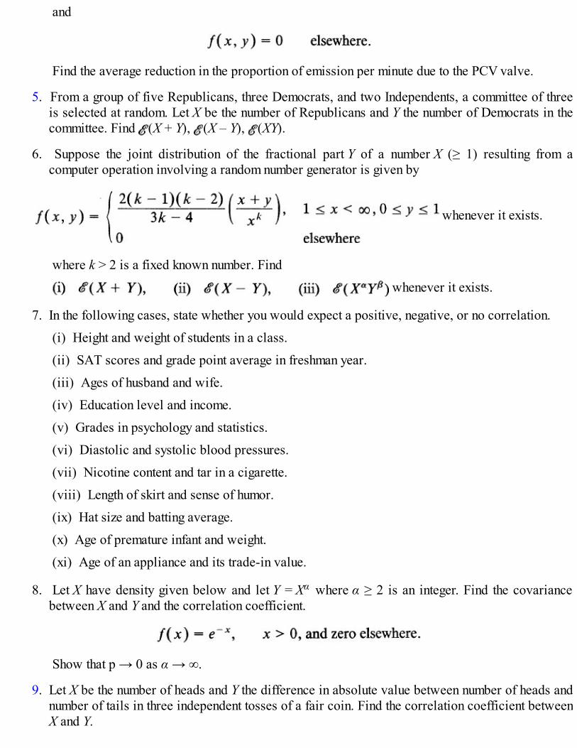
and

Find the average reduction in the proportion of emission per minute due to the PCV valve.

5. From a group of five Republicans, three Democrats, and two Independents, a committee of threeis selected at random. Let X be the number of Republicans and Y the number of Democrats in thecommittee. Find (X + Y), (X – Y), (XY).

6. Suppose the joint distribution of the fractional part Y of a number X (≥ 1) resulting from acomputer operation involving a random number generator is given by

whenever it exists.

where k > 2 is a fixed known number. Find

whenever it exists.

7. In the following cases, state whether you would expect a positive, negative, or no correlation.

(i) Height and weight of students in a class.

(ii) SAT scores and grade point average in freshman year.

(iii) Ages of husband and wife.

(iv) Education level and income.

(v) Grades in psychology and statistics.

(vi) Diastolic and systolic blood pressures.

(vii) Nicotine content and tar in a cigarette.

(viii) Length of skirt and sense of humor.

(ix) Hat size and batting average.

(x) Age of premature infant and weight.

(xi) Age of an appliance and its trade-in value.

8. Let X have density given below and let Y = Xα where α ≥ 2 is an integer. Find the covariancebetween X and Y and the correlation coefficient.

Show that p → 0 as α → ∞.

9. Let X be the number of heads and Y the difference in absolute value between number of heads andnumber of tails in three independent tosses of a fair coin. Find the correlation coefficient betweenX and Y.

10. Let X and Y have the joint density given below. Find the correlation coefficient between X and Y.

11*. Let X and Y be identically distributed random variables with probability function

(i) Show that .

(ii) Show that ρ = 1 if and only if P(X = Y) = 1 and ρ = –1 if and only if P(Y = N + 1 – X) = 1.[Hint: Use . See Problem 6.2.1 forproof. Note that

12*. Let X and Y have probability functions

and

Show that X and Y are independent if and only if ρ(X, Y) = 0.[Hint: Let U = aX + b, V = cY + d. From Proposition 3, ρ = 0 implies ρ(U, V) = 0. Use (2) toshow that U and V are independent by choosing a = 1, b = –x1 and c = 0, d = –y1.]

13. Let X and Y have common mean 0, common variance 1, and correlation coefficient ρ. Show that

[Hint: . Use Cauchy-Schwarz inequality.]

14*. In this problem, we ask the reader to show that cov( X, Y) exists but X2 is not finite (seeRemark 2). Suppose X is the length of time between successive demands for auto parts at a storewith density

where 1/y is the mean demand. Suppose Y itself is a random variable with density

(i) Show that cov(X, Y) exists and find cov(X, Y).(ii) Show that the unconditional density of X is

so that var(X) does not exist.

15*. Show with the help of the following joint density that (XY) may exist but even Y may not:

Show that(i) XY = 1. (ii) Y does not exist.

16. Let X be any random variable. Show that X is independent of itself if and only if P(X = c) = 1 forsome constant c.

5.3 LINEAR COMBINATIONS OF RANDOM VARIABLES

Let (X1 X2,…,Xm) be a random vector and let a1 a2,…,am be real numbers (not all zero). In statistics,linear combinations of the form occur quite often and we will find it convenient tocompute the mean and the variance of S. For example, if X1…,Xm is a random sample from a distributionfunction F, we have said that the statistic , which is the sample mean, is an intuitivelyappealing estimate of μ = μF. What are some properties of this estimate? What is its precision asmeasured by its variance? How do we use Chebyshev’s inequality to construct a confidence intervalestimate for μ based ?

THEOREM 1. Let X1 X2,…,Xm and Y1 Y2…,Yn be random variables with Xi = μi and Yi = ξi. Set

for real numbers a1,…,am and b1,…,bn. Then

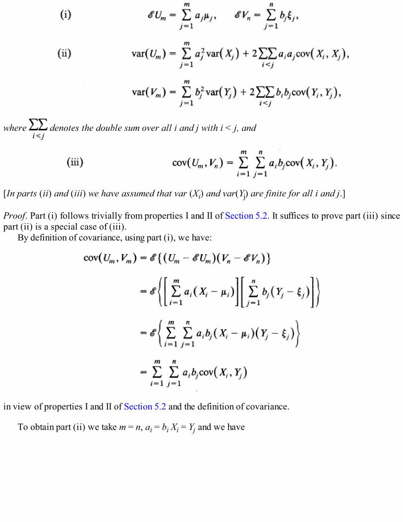
where denotes the double sum over all i and j with i < j, and

[In parts (ii) and (iii) we have assumed that var (Xi) and var(Yj) are finite for all i and j.]

Proof. Part (i) follows trivially from properties I and II of Section 5.2. It suffices to prove part (iii) sincepart (ii) is a special case of (iii).

By definition of covariance, using part (i), we have:

in view of properties I and II of Section 5.2 and the definition of covariance.

To obtain part (ii) we take m = n, ai = bi Xi = Yj and we have

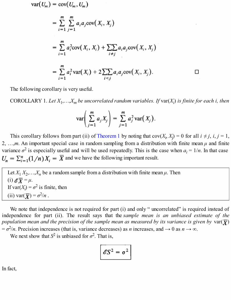
The following corollary is very useful.

COROLLARY 1. Let X1,…,Xm be uncorrelated random variables. If var(Xi) is finite for each i, then

This corollary follows from part (ii) of Theorem 1 by noting that cov(Xi, Xj) = 0 for all i ≠ j, i, j = 1,2, …,m. An important special case in random sampling from a distribution with finite mean μ and finitevariance σ2 is especially useful and will be used repeatedly. This is the case when ai = 1/n. In that case

and we have the following important result.

Let X1 X2,…,Xn be a random sample from a distribution with finite mean μ. Then(i) = μ.If var(Xi) = σ2 is finite, then(ii) var( ) = σ2/n .

We note that independence is not required for part (i) and only “ uncorrelated” is required instead ofindependence for part (ii). The result says that the sample mean is an unbiased estimate of thepopulation mean and the precision of the sample mean as measured by its variance is given by var( )= σ2/n. Precision increases (that is, variance decreases) as n increases, and → 0 as n → ∞.

We next show that S2 is unbiased for σ2. That is,

In fact,

Example 1. Sampling from a Finite Population, Consider a finite population II of N distinctelements ω1, ω2,…,ωN Frequently our object is to estimate the population mean

or the population variance

We take a simple random sample X1, X2,…,Xn of size n (≤ N) without replacement. Then X1, X2,…,Xn hasjoint probability function

where x1,…,xn ∈ Π. It is then natural to consider as an estimate of μ. How good is as an estimate ofμ We note that the marginal distribution of each Xj is given by

so that Xj = μ for each j. It follows from Theorem 1 (i) that is unbiased for μ, that is,

What about the precision of We have from Theorem 1 (ii)

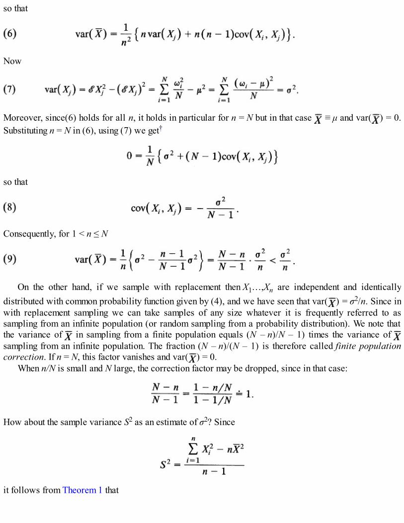
so that

Now

Moreover, since(6) holds for all n, it holds in particular for n = N but in that case ≡ μ and var( ) = 0.Substituting n = N in (6), using (7) we get†

so that

Consequently, for 1 < n ≤ N

On the other hand, if we sample with replacement then X1…,Xn are independent and identicallydistributed with common probability function given by (4), and we have seen that var( ) = σ2/n. Since inwith replacement sampling we can take samples of any size whatever it is frequently referred to assampling from an infinite population (or random sampling from a probability distribution). We note thatthe variance of in sampling from a finite population equals (N – n)/N – 1) times the variance of sampling from an infinite population. The fraction (N – n)/(N – 1) is therefore called finite populationcorrection. If n = N, this factor vanishes and var( ) = 0.

When n/N is small and N large, the correction factor may be dropped, since in that case:

How about the sample variance S2 as an estimate of σ2? Since

it follows from Theorem 1 that

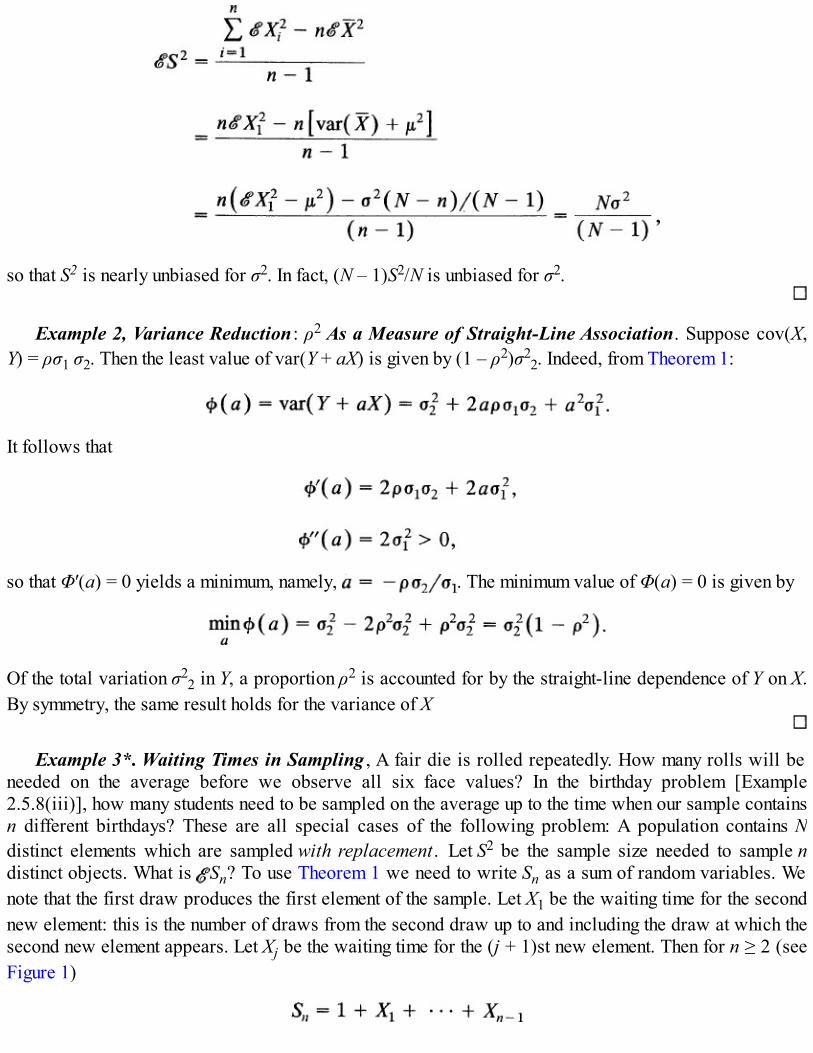
so that S2 is nearly unbiased for σ2. In fact, (N – 1)S2/N is unbiased for σ2.

Example 2, Variance Reduction : ρ2 As a Measure of Straight-Line Association. Suppose cov(X,Y) = ρσ1 σ2. Then the least value of var(Y + aX) is given by (1 – ρ2)σ2

2. Indeed, from Theorem 1:

It follows that

so that Φ′(a) = 0 yields a minimum, namely, . The minimum value of Φ(a) = 0 is given by

Of the total variation σ22 in Y, a proportion ρ2 is accounted for by the straight-line dependence of Y on X.

By symmetry, the same result holds for the variance of X

Example 3*. Waiting Times in Sampling , A fair die is rolled repeatedly. How many rolls will beneeded on the average before we observe all six face values? In the birthday problem [Example2.5.8(iii)], how many students need to be sampled on the average up to the time when our sample containsn different birthdays? These are all special cases of the following problem: A population contains Ndistinct elements which are sampled with replacement. Let S2 be the sample size needed to sample ndistinct objects. What is Sn? To use Theorem 1 we need to write Sn as a sum of random variables. Wenote that the first draw produces the first element of the sample. Let X1 be the waiting time for the secondnew element: this is the number of draws from the second draw up to and including the draw at which thesecond new element appears. Let Xj be the waiting time for the (j + 1)st new element. Then for n ≥ 2 (seeFigure 1)

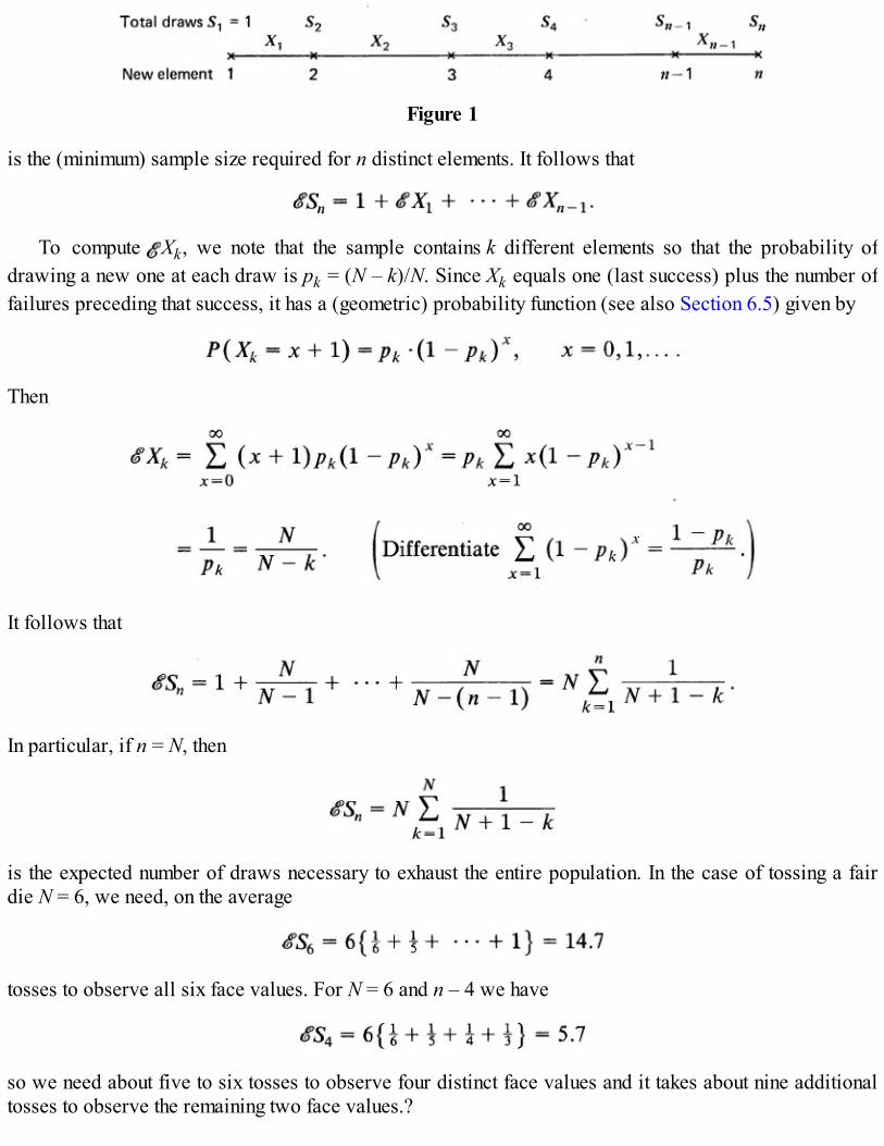
Figure 1

is the (minimum) sample size required for n distinct elements. It follows that

To compute Xk, we note that the sample contains k different elements so that the probability ofdrawing a new one at each draw is pk = (N – k)/N. Since Xk equals one (last success) plus the number offailures preceding that success, it has a (geometric) probability function (see also Section 6.5) given by

Then

It follows that

In particular, if n = N, then

is the expected number of draws necessary to exhaust the entire population. In the case of tossing a fairdie N = 6, we need, on the average

tosses to observe all six face values. For N = 6 and n – 4 we have

so we need about five to six tosses to observe four distinct face values and it takes about nine additionaltosses to observe the remaining two face values.?

We can approximate Sn by

If N = 365 and n = 25, then

so that we need to sample only 25 to 26 students on the average to observe 25 different birthdays.

Example 4. Confidence Interval for Population Mean μ. In Section 4.3 we saw that in order tocompute the numerical value of the minimum level 1 – α confidence interval for the population mean μ fora given sample, we either need to know the distribution of or we have to evaluate a multiple integral tocompute c1 and c2 such that

On the other hand, if we know a then we can compute a rough confidence interval estimate for μ at level atleast 1 – α by using Chebyshev’s inequality. Indeed, since = μ and var( ) = σ2/n we have fromChebyshev’s inequality

Choosing we get

which holds for all μ. Hence the confidence interval of level at least 1 – α is given by . If σ is unknown and n is large we can use S as an estimate of σ to get an

approximate confidence interval . For large n, however, we will see inChapter 9 that it is possible to do much better by using an approximation for the distribution of .

Remark 1. It is important to remember that we do not need to know the joint distribution of X1, X2,…,Xm to apply Theorem 1. We need only know the means of Xi, i = 1, 2,…,m in order to compute themean of any linear function of (X1,…,Xm). Similarly, if we know the variances var(Xj) andcovariances we can compute .

Example 5. Empirical Distribution Function As an Unbiased Estimate of the PopulationDistribution Function, Let X1, X2…,Xn be a random sample from distribution function F. Let bethe empirical distribution function of the sample. Define Yi = 1 if Xi ≤ x and Yi = 0 if Xi > x. Then Y1 Y2…,Yn are independent and identically distributed with common distribution

Moreover, Yj = F(x) and var(Yi) = F(x) – [F(x)]2. We note that

It follows that

for all x ∈ so that is an unbiased estimate of F(x).

Example 6. Estimating Covariance and Correlation Coefficient Given a random sample (x1, y1),(x2, y2),…,(xn, yn) of n observations on (X, Y), how do we estimate cov(X, Y) and ρ(X, Y)? We haveshown that and are unbiased estimatesof and respectively. This suggests that we consider

as an estimate of cov(X, Y). We show that S11 is an unbiased estimate. In fact

It follows that S11 = cov(X, Y) and S11 is unbiased.In order to estimate ρ(X, Y) we recall that

It is therefore natural to consider

as an estimate of ρ. The estimate R, however, is not unbiased for ρ. We note that S11 and R are consistentestimates of cov(X, Y) and ρ(X, Y) respectively (Problem 9.10.24). In Example 11.4.3 and Section 11.9we show how the statistic R is used in testing H0: ρ = 0. The statistic S11 is called the sample covarianceand R is called the sample correlation coefficient.

Example 7. Proportion of Faculty in Favor of Semester System. Suppose that at a certain stateuniversity a random sample of 65 faculty members is taken out of a total of 565 faculty members. Eachmember in the sample is asked the question, Are you in favor of or against the semester system? Theobject is to estimate the true proportion of faculty members who are in favor of the semester system.Suppose 35 of the respondents are found to be in favor of the proposition.

Let p be the true proportion of faculty members who are in favor of the semester system. Let Xi = 1 ifthe ith member of the sample responds with a yes and zero otherwise. Then

and according to Example 1, is an unbiased estimate of p with variance

where N = 565, n = 65, σ2 = var(Xi) = p – p2. Hence our point estimate of p is = 35/65 = .5385 and thevariance of the estimate is given by

Since p is unknown, we have two choices to estimate we can either replace p by in the expressionfor or use the unbiased estimate (N – 1)S2/N for σ2 (see Example 1). Writing for the estimate of when we replace p by we get

and

If we want a confidence interval estimate for p at level at least .95 say, we use Chebyshev’sinequality (as in Example 4). We have for all 0 ≤ p ≤ 1 with

Since is unknown we use instead to get an approximate confidence interval for p as

On the other hand, if we use (N – 1)S2/N to estimate σ2, then

so that

and = .0586. There is hardly any difference between the two estimates for .The important point to remember here is that the sampling is without replacement from a finite

population so that we need to use finite population correction in the computation of we do not do so,we will get a less precise confidence interval. Note also that in sampling from a finite population we dohave a natural lower bound for p. Indeed, . In sampling from an infinite population we donot have any such lower bound for p.

Approximation of Mean and Variance*

Let X, Y be jointly distributed random variables. If g is a linear function of X and Y, Theorem 1 shows ushow to compute the mean and the variance of g. For most practical purposes this result suffices. In someproblems, however, g is not linear. Suppose we wish to estimate the coefficient of variation σ/μ by, say,S/ . Is S/ unbiased? What is the variance of S/ ? Or, if the mean length of life of a piece of equipmentis 1/μ, we know that is unbiased for 1/μ. It is then natural to consider 1/ as an estimate of μ. How dowe find the variance of 1/ as an estimate of μ? Theorem 1 clearly does not apply here.

One possibility is to compute the distribution of g(X, Y). This is done in Chapter 8, where we see thatthe computation of distribution of g is often not simple. Even if we are able to compute the distribution ofg, the computation of variance or mean square error of g may not be easy. In any case, the procedure islong and complicated.

A second possibility, which is at least less time-consuming, is to compute g(X, Y) or var(g(X, Y))

directly from the distribution of (X, Y).In the case of most interest, however, X and Y will be some statistics based on one or more samples.

Neither of the above two procedures, in such cases, guarantees any success. We explore the thirdpossibility, that of finding approximations for g(X, Y) and var(g(X, Y)). We consider mainly theunivariate case.

THEOREM 2. Let g be a real valued function that is twice differentiable at x = θ. Then

and

Outline of Proof. Expanding g in a Taylor series about x = θ in two terms we have

where R is the remainder. R(X, θ) is discarded, then

which is (10).If we expand g in a Taylor series only to one term, then

and discarding R1 we get

COROLLARY 1. If then

and

It is possible to improve the approximation for by using (12) and higher-ordermoments of X. Similarly, an extension to two (or more) variables can be obtained by using Taylorexpansion for two (or more) variables. For example, if

, then under appropriate conditions on g,

and

We omit the details.

Remark 2. We emphasize that or varθ(g(X)) may not exist. These approximations do notassert the existence of mean and/or variance of g(X). For example, (S/ ) does not exist for somecommon distributions.

Example 8. Estimating p2 where p is Probability of a Success. Let X1, X2,…, Xn be a randomsample from probability function P(Xi, = 1) = p = P(Xi = 0). This is the coin tossing experiment with ahead (or success) identified as 1 and a tail as 0. Then is the proportion of heads (successes) in n trialsand = p, var( ) = p(1 – p)/n. (Here .) Supposewe wish to estimate g(p) = p2. Consider g( ) = 2 as an estimate of p2. We note that

so that from (13)

and

For large n, p(1 – p)/n is nearly zero and we see that g( ) = 2 is nearly unbiased for p2. We note that , so that the Taylor approximation gives an exact result

for g( ) in this case.

Example 9. Estimating the Gravitational Constant. In Example 1.2.1 we considered a simplependulum with unit mass suspended from a fixed point O (see Figure 2). Under the assumption that thependulum swings only under the effect of gravity we showed that the period of oscillation T = T(θ) as thependulum goes from θ = θ0 to θ = 0 is given by

Figure 2

and for a small oscillation

approximately. Suppose where ε is the random error with (ε) = 0. Then . How do we estimate g based on observable values T1, T2,…,Tn of T? We note that g =

c/T2 where c = 4π2. There are two obvious possibilities. For each observed Ti we get an observation gi,on g as c/Ti

2 and the average is then an estimate of g. (Here we are using the samenotation for the random variable c/T2 and the gravitational constant g.)

The second estimate can be obtained by first estimating T by so that

also estimates g.We have

and

Let Ti = μ and var(Ti) = σ2. In view of (13), and

and

Since we have

An application of (14) yields

As n → ∞ we note that is nearly unbiased for g but is positively biased.

Problems for Section 5.3

Problems 22-25 Refer to the Subsection.

1. A student takes a five-answer multiple choice test consisting of 10 questions. Suppose he or sheguesses at every question. What is the average number of his or her correct answers?

2. Let X1, X2,…,Xn be random variables with common mean μ and common variance σ2. Find:

3. In Problem 2, assume that the random variables, in addition, are uncorrelated. Find the variance ineach case.

4. Let var(X) = 2, var(Y) = 9, and cov(X, Y) = 2. Find:

5. A folding 4-foot ruler is constructed by joining four 12-inch pieces together. Suppose the piecesare chosen independently from a population with a mean length of 12 inches and standarddeviation σ. What is the mean length of the ruler and what is the variance of the length of a rulerconstructed in this fashion? If it is desired that the standard deviation of the length be .05 inches,what should be the value of σ

6. The profit that a company makes each quarter is a random variable with mean $100,000 andstandard deviation $20,000. If the profits each quarter are assumed independent and identicallydistributed, what is the average total profit for the year and the variance of total yearly profit?

7. Suppose X, Y have joint density given by:

Find the variance of Z = 3X + 2Y – 5.

8. Suppose X, Y, Z are random variables such that cov(X, Y) = 2, cov(X, Z) = – 2, var(X) = 6, var(Y)= 4, var(Z) = 9 whereas Y and Z are uncorrelated. Find cov(U, V) where U = X – 3Y + 2Z and V =–3X + 4Y + Z.

9. Suppose X and Y are two independent estimates of the true weight μ of an object. Assume X and Yare unbiased with finite variances and respectively.

(i) Show that for each α, αX + (1 – α)Y is also unbiased for μ.

(ii) How will you choose α to minimize the variance of αX + (1 – α)Y?

10. Let X, Y have joint density given by

Find:

11. Let X, Y and Z be jointly distributed random variables.(i) Show that cov( X + Z, Y) = cov(X, Y) + cov(Z, Y).(ii) Find the correlation coefficient between X + Y and X + Z when X, Y, Z are uncorrelated and

have the same variance.(iii) Find ρ(X + Y, X – Y) when X and Y are uncorrelated.(iv) Suppose X = Y and X2 = Y2. Show that cov(X – Y, X + Y) = 0.

12. Let X1, X2…,Xn be a random sample from a distribution with finite variance. Show that:

13. Let X1, X2…,Xn be a random sample from a distribution with Xi, = 0 = X3i.

Show that cov( , S2) = 0.

[Hint: Show that for each i.]

14. Let X1, X2…,Xn be dependent random variables with ρ(Xi, Xj) = ρ for i ≠ j, i, j = 1, 2,....,n Showthat – (n – 1)–1 ≤ ρ ≤ 1, when var(Xi) = var(Xj), for all i, j

15. Let X1, X2…,Xm + n be independent and identically distributed random variables with commonfinite variance σ2. Let . Find ρ(Sn, Sm + n – Sm) for n > m.

16*. A box contains D defective and N – D nondefective items. A sample of size n is taken withoutreplacement. Let X be the number of defective items in the sample. Show that

[Hint: Let Yi = 1 if ith item drawn is defective and Yi = 0 otherwise. Then . Showfirst P(Yi = 1) = D/N for i = 1, 2,…,n and P(Yi = 1, Yj = 1) = D(D – 1)/N(N – 1) for i ≠ j.]

17*. Let A1,…,Ak be disjoint events such that and P(Ai) = pi, 0 < pi < 1, . Inn independent trials of the experiment, let X1, X2…,Xk denote the number of times that A1, A2,…,Ak occur, respectively. Then . Show that .[Hint: Let Ul = 1 if lth trial results in Ai and zero otherwise. Let Vm = 1 if mth trial results in Ajand zero otherwise. Then and . Use Theorem 1 (iii).]

18*. Consider a dichotomous experiment with a probability of success p. The experiment is repeatedindependently until r successes are observed. Let Y be the number of trials required to observe rsuccesses. Show that Y = r/p and var(Y) = r(1 – p)/p2. [Hint: Define Xi = trial number onwhich ith success is observed, i = 1, 2,…,r and Wi = Xi – Xi – 1, i = 1, 2,…,r, with X0 = 0. ThenWi are independent identically distributed random variables and

. The probability function of W, is given by P(Wi = w)= p(1 – p)w – 1, w = 1,2,….]

19*. A box contains N items of which Dj are of jth type, randomsample of size n is taken without replacement. Let be the number of items of type i, i = 1,…,k.Then . Show that for i ≠ j, cov(Xi, Xj) = –nDiDj(N – n)/[N2(N – 1)]. [Hint: Let Ul =1 if lth draw is of type i and zero elsewhere, and let Vm = 1 if mth draw is an item of type j andzero elsewhere. Then Ul = Dj/N, Vm = Dj/N and UlVm = DiDj/N(N – 1), for l ≠ m, UlVl =0.]

20. Let X1, X2,…,Xm and Y1,…,Yn be independent random samples from distributions with means μ1and μ2 and variances and respectively. Show that:

21. In Problem 20, let S21, S2

2 be the two sample variances. Show that

In particular, if σ1 = σ2 = σ show that

is unbiased for the common variance σ2. In this case, two other unbiased estimates are S21 and

S22. Which of the three do you think should be preferred and why?

22*. Let X1, X2,…,Xn be a random sample from a distribution with finite mean μ and finite varianceσ2. It is required that g(μ) be estimated by g( ). Find approximate expressions for g( ) andvar(g( )). In particular, consider the function g(x) = x2. Obtain expressions for 2 and var(2).

23*. Let X1 X2,…,Xn be a random sample from probability function

An estimate of var(Xi) = p(1 – p) is required. Consider the estimates , and . Compute approximate expressions for the means and the variances.

[Hint: Note that S2 is unbiased for σ2. Write where . Then

.]

24*. According to Ohm’s law, the voltage Fin a simple circuit can be expressed as V = IR, where I isthe current and R the resistance of the circuit. Suppose I and R are independent randomvariables. Use (15) and (16) to show that

(Note that V = I R by independence of I and R.)

25*. Frequently it is of interest to estimate μ1/μ2 where μ1, μ2 are means of two random variables Xand Y with variances and , respectively. Let X1…,Xm and Y1…,Yn be independent randomsamples. Consider the estimate X/Y. Show, using

and

In the special case when m = n, consider the estimate . Find approximations forits mean and the variance.

5.4 THE LAW OF LARGE NUMBERS

We defined probability of an event A as a measure of its uncertainty, that is, as a measure of how likely A

is to occur. Our intuitive notion of probability is based on the assumption that it is a long-term relativefrequency of occurrence of A. That is, if the experiment is repeated n times under identical conditions andA occurs N(A) times, then N(A)/n should be close to P(A), the probability of A. When we say that P(A) isthe probability of A on a particular trial we are applying to this particular trial a measure of its chancebased on what would happen in a long series of trials. Thus when a fair coin is tossed five times andshows five heads, the probability of a tail on the next toss is still 1/2. The so-called (and generallymisinterpreted) law of averages does not demand that the sixth, seventh, or eightth trials produce tails tobalance the five straight heads. If a surgeon performs a delicate surgery where the chances of success areonly 1 in 10, it should be no comfort to the tenth patient that the previous nine operations were failures. Ifa couple has had six girls in a row, the probability that the seventh child will be a girl is still 1/2. It istrue that the probability of seven straight girls (= 1/27 = .008) is small but given that the first six childrenborn to them were girls, the probability of the seventh being a girl is 1/2.

We now give a precise formulation of the law of averages (it is called the law of large numbers). Weconsider only a weak version of the law of large numbers.

Law of Large Numbers

Let {Xn} be a sequence of independent random variables with a common distribution and let Xn = μ, exist. Then for every ε > 0 as n → ∞

that is, the probability that the sample average will differ from the population expectation by lessthan ε (arbitrary) approaches one as the sample size n → ∞.

Unfortunately, even this version is beyond our scope. We prove the following result instead.

THEOREM 1. Let {Xn} be a sequence of random variables. Suppose var(Xj) = εj2 is finite for each as n → ∞ then for every ε > 0 as

Proof. From Chebyshev’s inequality

as n → ∞.

COROLLARY 1. If Xn’s are uncorrelated and identically distributed with common finite

variance σ2, and Xj = μ, then for every ε > 0 as .

Proof. Since Xn’s are uncorrelated, it follows from Theorem 5.3.1 that

and hence

as n → ∞.

In particular, if the Xi’s are independent and identically distributed (as in the case of randomsampling) with finite variance, then the sample mean is likely to be close to μ for large n. That is, isa consistent estimate of μ. This provides yet another justification for using sample mean as an estimate ofμ. (We do not need the existence of variance in this special case but the proof is beyond our scope.) In therest of this text, when we speak of the law of large numbers we refer to Corollary 1 above.

Remark 1. The law of large numbers asserts only that for every particular sufficiently large n thedeviation | – μ| is likely to be small. It does not imply that | – μ| remains small for all large n.

Remark 2. The law of large numbers as proved above makes no assertion that P| → μ| = 1. It assertssimply that is likely to be near μ for every fixed sufficiently large n and not that is bound to stay nearμ, if n is increased. Actually, it is true that with probability one | – μ| becomes small and remains smallin random sampling from a distribution with finite mean, but we will not prove it here or use itsubsequently. This is the so-called strong law of large numbers.

Example 1. Relative Frequency of an Event A is likely to be Near P(A). Consider an event withprobability P(A). Suppose in n independent trials of the experiment, A occurs N(A) times. Then therelative frequency of A is R(A) = N(A)/n. We show that N(A)/n is likely to be near P(A). That is, R(A) is aconsistent estimate of P(A).

Define Xi = 1 if A occurs on the ith trial and Xi = 0 otherwise. Since the trials are independent, Xi’sare independent and, moreover, Xi = P(A), var(Xi) = P(A)[1 – P(A)]. Also

so that . By the law of large numbers, for every ε > 0 as n→ ∞

as asserted.

Example 2. Error in Estimation and Sample Size Determination. Let X1, X2,…, Xn be a randomsample from a distribution with mean μ and variance σ2. According to the law of large numbers

as n → ∞ for every ε > 0 where . In other words,

so that the law of large numbers tells us that Sn grows at rate n. We can use the law of large numberseither to find an error bound in estimating μ by or to find the sample size n required given an errorbound. Thus the error in estimation is at most ε with probability at least . Indeed,

On the other hand, if we want the error to be at most ε with a probability of at least 1 – α, then we choosen from

giving . We will see that we can do much better with the help of the central limit theorem(see Section 9.3).

Example 3. The Empirical Distribution Function. Let X1,…,Xn be a random sample from adistribution function F. We recall that the empirical distribution function of the sample is defined by

Let

In Example 5.3.6 we saw that Y1, Y2,…,Yn are independent and identically distributed with

and

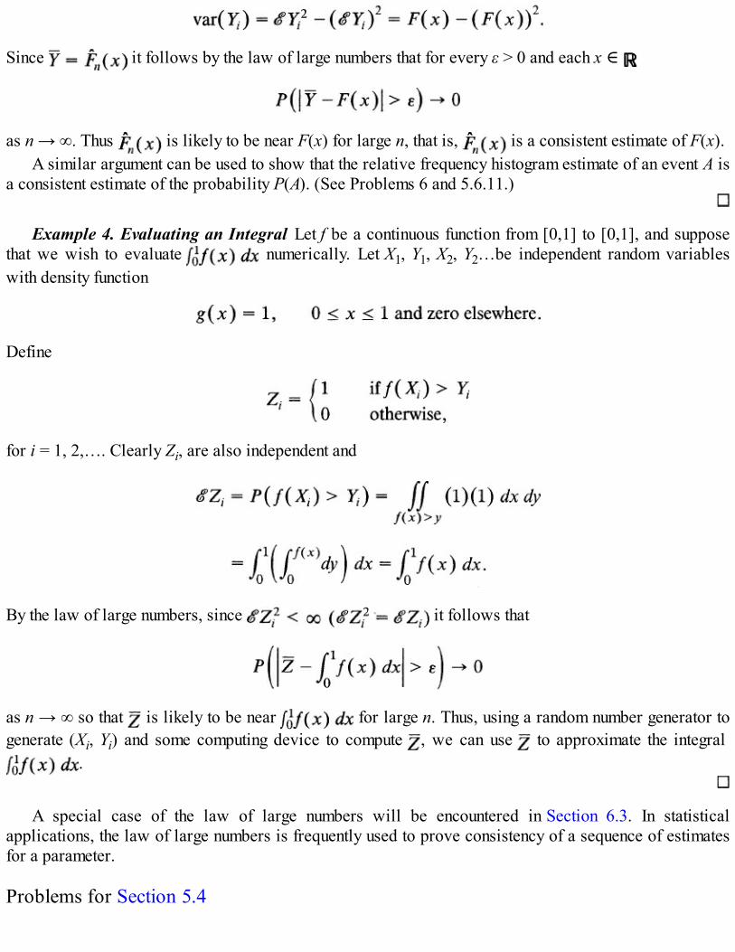
Since it follows by the law of large numbers that for every ε > 0 and each x ∈

as n → ∞. Thus is likely to be near F(x) for large n, that is, is a consistent estimate of F(x).A similar argument can be used to show that the relative frequency histogram estimate of an event A is

a consistent estimate of the probability P(A). (See Problems 6 and 5.6.11.)

Example 4. Evaluating an Integral Let f be a continuous function from [0,1] to [0,1], and supposethat we wish to evaluate numerically. Let X1, Y1, X2, Y2…be independent random variableswith density function

Define

for i = 1, 2,…. Clearly Zi, are also independent and

By the law of large numbers, since it follows that

as n → ∞ so that is likely to be near for large n. Thus, using a random number generator togenerate (Xi, Yi) and some computing device to compute , we can use to approximate the integral

.

A special case of the law of large numbers will be encountered in Section 6.3. In statisticalapplications, the law of large numbers is frequently used to prove consistency of a sequence of estimatesfor a parameter.

Problems for Section 5.4

1. Let X1, X2…. be a sequence of independent random variables with distribution given below.Does the sufficient condition of Theorem 1 hold in each case? (If , it does notfollow that the law of large numbers does not hold.)

2. Suppose X1 X2,…,Xn is a random sample with finite mean μ and finite variance σ2. Show that

as n → ∞. That is, is a consistent estimate for μ. (Hint: Use Theorem 5.3.1and Theorem 1 of this chapter.)

3. Suppose {Xn} is a sequence of random variables with common finite variance σ2. Suppose ¿sothat for all i ≠ j, cov(Xi, Xj) < 0. Show that the law of large numbers holds for {Xn}.

4. Suppose X1, X2… are independent, identically distributed with for some positiveinteger k. Show that

the unbiased estimate of (for 1 ≤ 7 ≤ k) is likely to be near for large n. That is, showthat

as n → ∞ for every ε > 0 .

5*. Let {Xn} be such that Xj is independent of Xk for k ≠ j + –1 or k ≠ j – 1. Suppose 0 < var(Xn) < cfor all n and some constant c. Show that {Xn} obeys the law of large numbers.

6. Let x1 x2,…,xn be n observations from a known density function f. Let us construct a histogram ofthe data by subdividing the real line in disjoint intervals (aj, aj + 1), j = 0,1,… . Let fj be the classfrequency of (aj, aj + 1) and be the histogramestimate of f. Let be the histogram estimate of P(A). Show that

as n → ∞ for every ε > 0, whenever A is a union of intervals

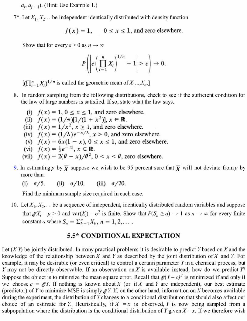
aj, aj + 1). (Hint: Use Example 1.)

7*. Let X1, X2… be independent identically distributed with density function

Show that for every ε > 0 as n → ∞

[ is called the geometric mean of X1...,Xn.]

8. In random sampling from the following distributions, check to see if the sufficient condition forthe law of large numbers is satisfied. If so, state what the law says.

9. In estimating p by suppose we wish to be 95 percent sure that will not deviate from μ bymore than:

Find the minimum sample size required in each case.

10. Let X1, X2,… be a sequence of independent, identically distributed random variables and supposethat Xi = μ > 0 and var(Xi) = σ2 is finite. Show that P(Sn ≥ a) → 1 as n → ∞ for every finiteconstant a where

5.5* CONDITIONAL EXPECTATION

Let (X Y) be jointly distributed. In many practical problems it is desirable to predict Y based on X and theknowledge of the relationship between X and Y as described by the joint distribution of X and Y. Forexample, it may be desirable (or even critical) to control a certain parameter Y in a chemical process, butY may not be directly observable. If an observation on X is available instead, how do we predict Y?Suppose the object is to minimize the mean square error. Recall that (Y – c)2 is minimized if and only ifwe choose c = Y. If nothing is known about X (or if X and Y are independent), our best estimate(predictor) of Y to minimize MSE is simply Y. If, on the other hand, information on X becomes availableduring the experiment, the distribution of Y changes to a conditional distribution that should also affect ourchoice of an estimate for Y. Heuristically, if X = x is observed, Y is now being sampled from asubpopulation where the distribution is the conditional distribution of Y given X = x. If we therefore wish

to estimate Y to minimize MSE, this estimate should be the expected value of the conditional distribution.Let X, Y be jointly distributed. We recall that

whenever P(X = x) > 0, defines a probability mass function for each fixed x (as a function of y) provided(X, Y) is of the discrete type. In the continuous case

defines a probability density function for each fixed x (as a function of y) where f is the joint and f1 themarginal density of (X, Y) and X respectively.

Clearly, then, for fixed x we can define the expected value of Y in this subpopulation just as wedefined g(X).

DEFINITION 1. Suppose X and Y are discrete type random variables. We define the conditionalexpectation of Y given X = x by:

and that of X given Y = y by:

provided the sums converge absolutely.If X and Y have a joint density function f, then we define

and

provided the integrals converge absolutely. Here g and h are respectively the conditional densities of Ygiven X = x and X given Y = y.

If one of X and Y is a discrete type while the other is a continuous type, we define {X| Y = y) and {Y|X = x) in an analogous manner. Similarly we can define {Φ(X)|Y = y} or {Φ(Y)|X = x} for anyfunction Φ.

Example 1. Sampling Inspection. A lot contains 10 items, two of type A, four of type B, and four oftype C. A sample of size two is drawn without replacement. Let

Then the joint distribution of (X, Y) is given by the probability function:

Clearly

so that

Similarly,

and

Also:

so that

and

Example 2. Standby-Redundant System. Consider a standby-redundant system. Each component insuch a system operates continuously until it fails, and then it is immediately replaced by a standbycomponent which operates until it fails. Components can fail while in use.

Let X, Y respectively denote the failure times of the original and the standby component as measuredfrom time 0 when the system is switched on. Then Y ≥ X. Suppose (X, Y) have joint density

where α ≠ β and α > 0, β > 0. It is easy to check that the marginal densities of X and Y are given,respectively, by

and

Then

It follows that

Similarly,

for 0 < x ≤ y , and zero for x > y. Hence

on integration by parts. It follows that

We note that as x varies, {Y|X = x} varies, and we can think of {Y|X = x} as a random variable thatassumes the value {Y|X = x} when X = x. Similarly, {X|Y} is a random variable with distribution P(Y =y) or f2(y) depending on whether Y is a discrete or continuous type. We can therefore speak of theexpected value of {X|Y}, and so on.

THEOREM 1. I f |X| < ∞, then {X|Y = y} is finite for every y for which the conditionaldistribution of X given Y = y is defined. Moreover,

Proof. We shall prove the result in the discrete case only. A similar proof holds for the continuous case.Suppose P(Y = y) > 0. Then P{X = x|Y = y) is defined, and moreover:

It follows that

In that case,

as asserted. The interchange of summation signs is justified because of absolute convergence. ESimilarly, if |Y| ≤ ∞ then

Both (1) and (2) are very useful, as we shall see. We emphasize that {X|Y} may be finite without Xbeing finite.

We first state some properties of conditional expectations. For convenience we shall write {X|y} for{X|Y = y}. In the following we assume that the indicated expectations exist.

PROPOSITION 1.

(i) If X and Y are independent and |X| ≤ ∞ then

and if |Y| ≤ ∞, then

(ii) Let Φ(X, Y) be a function of X and Y. Then

and

Moreover,

for any functions Φ1 and Φ2 and real numbers α1, α2.(iii) If Ψ is a function of X and Φ a function of X and Y, then

We leave it to the reader to supply a proof of Proposition 1.

Example 3. Sum of Random Number of Independent Random Variables . Let X1, X2,… beindependent and identically distributed random variables and let N be a positive integer valued randomvariable that is independent of the X’s. Set . What is SN? We note that SN has N termswhere N itself is a random variable. We cannot apply Theorem 5.3.1 to compute SN.

Random variables such as SN arise often in practice. For example, suppose the number of customersper day who shop at a store is a random variable N. Let X be a consumer’s demand for a certain item. LetX1…,Xn… be independent and identically distributed and suppose N is independent of X. Then theexpected consumer demand for this item at this store per day is (X1 + X2 + … + XN).

Suppose |Xi| < ∞ and N < ∞. Now SN = Sn when N = n is observed. We use (1) and have

Actually, we first need to check that |SN| < ∞ before we can apply (1). But this is easily done byreplacing SN by |SN| using triangular inequality and the fact that |Xi| < ∞ and N < ∞.

Note how Theorem 5.3.1 is modified when N is a random variable. We simply replace n by N in Sn = n Xi This result is called Wald’s equation and has many applications.

Example 4. {Y|X) May Exist but Y May Not. Consider the joint density function

of Problem 5.2.15. We note that

Clearly, does not exist (that is, is not finite), but

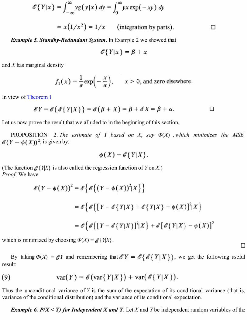
Example 5. Standby-Redundant System. In Example 2 we showed that

and X has marginal density

In view of Theorem 1

Let us now prove the result that we alluded to in the beginning of this section.

PROPOSITION 2. The estimate of Y based on X, say Φ(X) , which minimizes the MSE , is given by:

(The function {Y|X} is also called the regression function of Y on X.)Proof. We have

which is minimized by choosing Φ(X) = {Y|X}.

By taking Φ(X) = Y and remembering that , we get the following usefulresult:

Thus the unconditional variance of Y is the sum of the expectation of its conditional variance (that is,variance of the conditional distribution) and the variance of its conditional expectation.

Example 6. P(X < Y) for Independent X and Y. Let X and Y be independent random variables of the

continuous type. Then P(X < Y) is of great interest in statistics. For example, let X and Y be lifetimes oftwo components operating independently. Then P(X < Y) is the probability that the second component(with lifetime Y) survives the first component (with lifetime X). Now, if IA is the indicator function of setA, then

by Theorem 1. We note that

where Fx is the distribution function of X. Hence

where fY is the density function of Y. In particular, if fX = fY then

on integration by parts.More generally,

which gives the distribution function of X – Y.

Example 7. Trapped Miner. Consider a miner trapped in a mine with three doors. The first doorleads to a tunnel with no escape and returns him to his cell in the mine in one hour. The second door alsoleads to a tunnel with no escape and returns him to his cell in the mine in three hours. The third door takeshim to safety in one hour. If the miner at all times chooses randomly from the untried doors, what is theexpected length of time until he reaches safety?If we let X denote the time he takes to make good his escape and let Y1 denote the door he choosesinitially, then

where Y2 denotes the door he chooses on the second try. Then

This follows since the miner having chosen door 1 on the first try returns to the mine after one hour andthen chooses door 2 or door 3. If he chooses door 2, then he spends three hours in the tunnel, returns, andtries door 3, which leads him to safety in one additional hour. On the other hand, if he chooses door 3 onthe second try, he reaches safety in an hour. Similarly,

It follows that

An alternative approach would be to evaluate X directly, bypassing the conditional expectationapproach. We note that the only possible door sequences are 123, 213, 23, 13, 3 with respective totaltimes required to reach safety (in hours) 5, 5, 4, 2 and 1. Hence

For a somewhat simpler (but unrealistic) model, see Problem 3.

Example 8. Estimating Proportions of Two Chemicals in a Compound. Let X and Y denote theproportions of two different chemicals in a sample from a chemical mixture with joint density function

Then (see Figure 1)

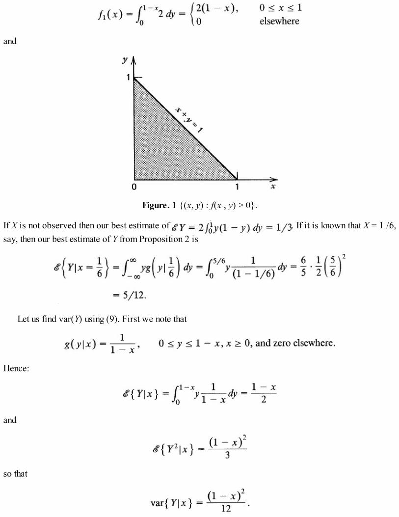
and

Figure. 1 {(x, y) : f(x , y) > 0}.

If X is not observed then our best estimate of . If it is known that X = 1 /6,say, then our best estimate of Y from Proposition 2 is

Let us find var(Y) using (9). First we note that

Hence:

and

so that

It follows that and

and

Hence from (9)

In this case it is simpler to compute var(Y) directly from f2(y).To summarize what we have done in this example, the best predictor of Y when no information on X is

available is Y = 1/3. This estimate minimizes (Y – c)2. If, on the other hand, it is known that X = 1/6,then our best predictor of Y is {Y|X = 1/6} = 5/12 in the sense that it minimizes {Y – Φ(X)}2. In eachcase we minimize the average of the squared deviation between Y and its estimate.

Problems for Section 5.5

1. Each word in the sentence I DO NOT LIKE THIS GLASS is written on a slip and the six slipsare returned to a box. A slip is then randomly selected. Let X be the length of the word on the slipdrawn and Y the number of I’s in the selected word. Find

.

2. Let X, Y be jointly distributed with probability function

Find .

3. A prisoner has just escaped from jail. There are three roads that lead away from the jail, A, B,and C. Of the three, C leads to freedom immediately and the other two lead back to the prisongate in 15 minutes. If at all times the prisoner selects roads A, B, and C with probability 1/2, 1/3,and 1/6, what is the expected time that it will take to make good the escape?

4. A fair coin is tossed three independent times. Let X be the number of heads and Y the number ofhead runs, where a head run is defined to be a consecutive occurrence of at least two heads.Check that the joint probability function X and Y is given by:

Find ({Y|x} and {X|y}.

5. Let X be the sum of face values and Y the numerical difference between face values when a pairof dice is tossed once. The joint probability function of (X, Y) is given below.

Find

6. Compute {X|Y} and {Y|X} for each of the following bivariate densities:

7. For the joint density

of X and Y, show that .

8. Let (X, Y) have joint density given by

Show that the best estimate of an Xvalue given Y = y is given by (5 – 4y)/(8 – 6y).

9. Let (X, Y) have joint density function given below.

Find, in each case, .

10. Find XY by conditioning on X or Y in each of the following cases:

11. Let T be the failure time of a component that is tested until failure at various voltage levels. Thefailure time is found to have a mean directly proportional to the square of the voltage. If thevoltage has density

find the average time to failure of the component.

12. A point X is chosen from the interval [0,1] according to density

Another point Y is chosen from the interval [0, X] according to the density

Find {Yk |x } and {Yk }, where k > 0 is a fixed constant.

13. Let X and Y be independent continuous random variables.

14. Let X1, X2,… be independent identically distributed and let N be a nonnegative integer valuedrandom variable which is independent of the X’s. Show that

provided X2 < ∞ and N2 < ∞. [Hint: Use (9). Alternatively, proceed directly as in Example3.]

15. Show that the MSE of the predictor {Y|X) of Y is given by (var{Y|X}).

16*. Consider a battery that is installed in a process and operates until it fails. In that case it isimmediately replaced by another battery, and so on. The process continues without interruption.Let F be the lifetime distribution of the battery. Let N(t) be the number of batteries that fail bytime t. Show that the battery in use at any time t tends to have a longer life length than anordinary battery. That is, show that

[Hint: Let is the length of the battery inuse. SN(t) is the time at which the last battery was replaced prior to t.

Condition on SN(t). Then . Show that if s > x and =

17*. Let X1, X2,…,Xn be exchangeable random variables. Show that

for j ≠ k, and hence conclude that

Given X1 + … + Xn = z, what is the best predictor of X1? (X1, X2, … ,Xn are exchangeable if theirjoint distribution F(x1, x2,…,xn) remains unchanged under any permutation of the arguments x1

x2…,xn.)

18. Let X, given = λ, have probability function

and suppose has density function

Find .

19*. Let (X, Y) be jointly distributed. Suppose X is observable and we wish to predict Y by Φ(X) inorder to minimize |Y – Φ(X)|. What is the best predictor Φ(X)? (Hint: Use Problem 3.7.25.)

5.6 REVIEW PROBLEMS

1. Two particles have lifetimes X and Y with joint density function given by

(i) Find (Y – X) and var(Y – X).

(ii) Find {Y|x} and {X|y}.

(iii) Verify that by using part (ii).

2. Let X and Y have joint density given by

(i) Find cov(X, Y) and ρ(X, Y)

(ii) Find var(2X + 7Y).

(iii) Find { X|y = 1/2}.

3. A random sample of 40 students is taken from a small college student body that has 450 students.Each student in the sample is asked if he or she is for or against Saturday morning classes.Suppose eight students are in favor of the proposal. Find an estimate of the true proportion ofstudents at this college favoring the proposal. Find an estimate for the variance of your estimateand a 95 percent confidence interval for the true proportion using Chebyshev’s inequality.

4. In Examples 5.2.1, 5.2.4, and 5.2.7, the joint distribution of the total time X that a customerspends in a bank and the time Y spent standing in line was assumed to have density function

What is the variance of the service time X – Y?

5. Let X ≥ 1 be a real number and let Y be its fractional part. Suppose X and Y are jointly distributed

with density function

(i) Find {Y|X) and Y.

(ii) Find var{Y|X}.

6. Consider a randomly selected family with six children. Let Xi = 1 if the i th oldest child is a girland zero otherwise. If it is known that the family has five girls, what is {X1|Y = 5} where Y isthe number of girls in a family with six children?

7. Let (X, Y) be the coordinates of a spot on the circular section of a radar station and suppose (X, Y)has joint density function

(i) Find {X|Y}, X, and var{X|Y}.

(ii) Find {X + Y}, (XY), and ρ(X, Y).

(iii) Find var(X + Y).

(See also Examples 3.4.4 and 3.5.3.)

8. The surface tension X and the acidity Y of a certain chemical compound are jointly distributed withdensity function

(i) Find {X|Y} and var{X|Y}.

(ii) Find cov( X, Y) and ρ(X, Y).

(iii) Find var(X + Y).

(See also Problem 3.5.10.)

9. The best mean square error predictor of Y is Y when nothing is known about X. The best meansquare predictor of Y given X = x is given by the conditional mean {Y|X = x} (Proposition5.5.2). Often one does not know how to find {Y|x}. In that case, one may be content to use thebest linear predictor a + bX where a and b are chosen to minimize the mean square error (Y – a– bX)2.

(i) Show that

so that the best linear predictor of Y is given by

where ρ is the correlation coefficient and σ1, σ2 are the standard deviations of X and Yrespectively.

(ii) Show that the minimum mean square error is σ22(1 – σ2). (See also Example 5.3.2.) [The

predictor in (i) is called the linear regression of Y on X.]

10. Suppose one word is randomly selected from the sentence IT IS NOT YET TIME TO GOHOME. Let Y be the number of letters in the word selected.

(i) What is your best estimate of the length of the word selected in the sense of minimum variance(or mean square error)?

(ii) Let X be the number of letters E in the word selected. Suppose you know that X = 1. What isyour best estimate of Y in the sense of minimum mean square error?

(iii) Suppose you wish to use a linear predictor α + bX for Y. What is your best predictor?

(iv) Find the mean square error in each case.

11. Let be the histogram estimate of f(x) for

(i) Show that for

where F is the distribution function corresponding to f, and

(ii) as n → ∞

By the mean value theorem for some xj ∈ (aj – 1, aj) sothat is an unbiased and consistent estimate of xj in (aj – 1, aj)

12. A process produces a proportion p of defective items where p is unknown. A random sample ofsize n is to be taken in order to estimate p by the sample proportion of defective items. If theerror in estimation is not to exceed .01 with probability at least .90, how large should the samplesize be?

13*. The area X of triangle ABC is given by the relation X = (ab/2)sinγ where γ is a random variablehaving uniform distribution on (0, θ). Find approximate expressions for the mean and varianceof X.

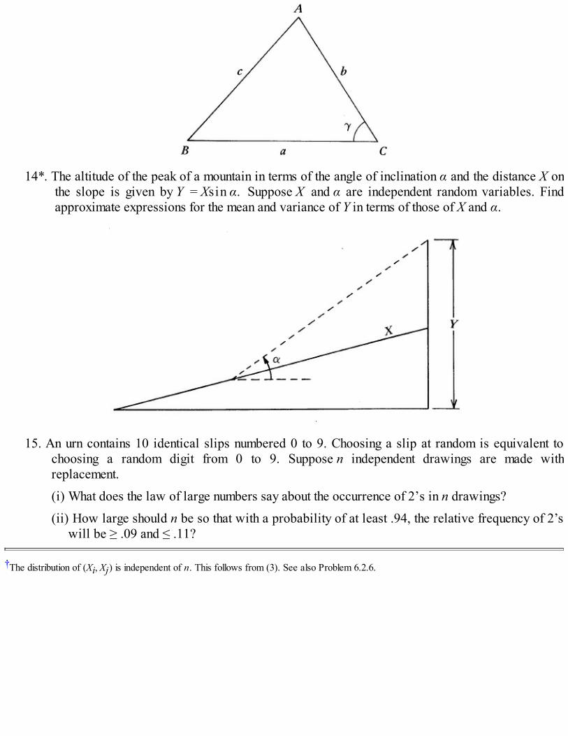
14*. The altitude of the peak of a mountain in terms of the angle of inclination α and the distance X onthe slope is given by Y = Xsin α. Suppose X and α are independent random variables. Findapproximate expressions for the mean and variance of Y in terms of those of X and α.

15. An urn contains 10 identical slips numbered 0 to 9. Choosing a slip at random is equivalent tochoosing a random digit from 0 to 9. Suppose n independent drawings are made withreplacement.

(i) What does the law of large numbers say about the occurrence of 2’s in n drawings?

(ii) How large should n be so that with a probability of at least .94, the relative frequency of 2’swill be ≥ .09 and ≤ .11?

†The distribution of (Xi, Xj) is independent of n. This follows from (3). See also Problem 6.2.6.

CHAPTER 6

Some Discrete Models

6.1 INTRODUCTION

A number of random experiments can often be modeled by the same stochastic model. The conditionsunderlying the experiment often fit a pattern for which a specific model may be applicable. In Chapters 6and 7 we consider some examples of probability models that are very useful in practical applications ofprobability and statistics.

In this chapter we consider some discrete integer-valued stochastic models. Section 6.2 deals with thediscrete uniform model, which has many applications, such as simple random sampling (Section 2.8).

Several models result when we seek answers to certain questions concerning a sequence ofindependent repetitions of a random experiment. Suppose for each repetition we are interested only inwhether an event A does or does not occur. Each occurrence of A is usually called a success. Let p = P(A)and set Xi = 1 if the ith trial is a success and Xi = 0 otherwise. Typical examples are coin tossing games,observing the sex of newborns in a hospital, observing whether or not a new drug is effective, and so on.Suppose there are n repetitions (trials). What is the probability of observing k successes, k = 0, 1, 2, …,n? The random variable of interest here is and we seek P(Sn = k) for k = 0, 1, …, n. Themodel {P(Sn = k;), k = 0, 1, … n} is called a binomial model and is the subject of discussion in Section6.3. We also consider inferential questions concerning p for the case when n is small.

If, on the other hand, we seek the distribution of the number of trials necessary to achieve the first(rth) success, then the resulting model is known as a geometric (negative binomial) model. This is studiedin Section 6.5.

In the binomial case, if n is large and p is small then one can use an approximating model calledPoisson model. Poisson models are used to characterize rare events. Typical examples are the number ofaccidents at an intersection during a certain period, and the number of telephone calls received during a15-minute interval. Section 6.6 deals with Poisson models.

Section 6.4 deals with the hypergeometric model that arises in practice in sampling (withoutreplacement) from a finite population. This is the case, for example, in lot inspection. A lot contains Nitems of which D are defective. A sample of size n is taken and inspected. What is the probability that thesample contains X defectives? A typical application of the hypergeometric model is in estimating the sizeof an animal population by the following capture-recapture procedure. A sample of size D is captured,tagged, and then released into the population. After some time a new sample of size n is taken, and thenumber of tagged animals is counted.

I n Section 6.7 we consider two multivariate models that are generalizations of binomial andhypergeometric models.

In spite of the length of this chapter, it can and should be covered rather quickly. The reader shouldconcentrate mostly on the model assumptions and applications and on the inferential techniques developedin each section. The reader should already be familiar with routine summations to show whether afunction is a probability function or with the computation of moments of a probability function. These areincluded here for completeness and easy accessibility.

6.2 DISCRETE UNIFORM DISTRIBUTION

Consider an experiment that can terminate in N mutually exclusive events Al, A2, …, An, all equally likely.Let be the sample space of the experiment. Clearly P(Ak) = 1/N, k = 1, 2, …, N. Let usdefine a random variable X on Ω as follows:

Then the probability function of X is given by

A random variable X with probability function (1) is said to have a uniform distribution on {xl, x2, …xN}. For example, in a single throw with a fair die, if we let X be the face value on the side that shows upthen X has uniform distribution on (1, 2, 3, 4, 5, 6} with probability function

For a random variable with probability function (1) we have

In particular

and so on. In the special case when xi = i, i = 1, 2, …, N

The generation of samples from a uniform distribution is facilitated by the use of a table of randomnumbers (Table A1 in the Appendix), as we saw in Chapter 2. The most important application of theuniform distribution, as we have seen, arises in sampling from a finite population. Indeed (in unorderedsampling without replacement), a sample is a simple random sample of size n from a population of Nobjects if each of the possible samples has the same probability of being drawn, namely,

That is, the distribution of samples is uniform with probability function

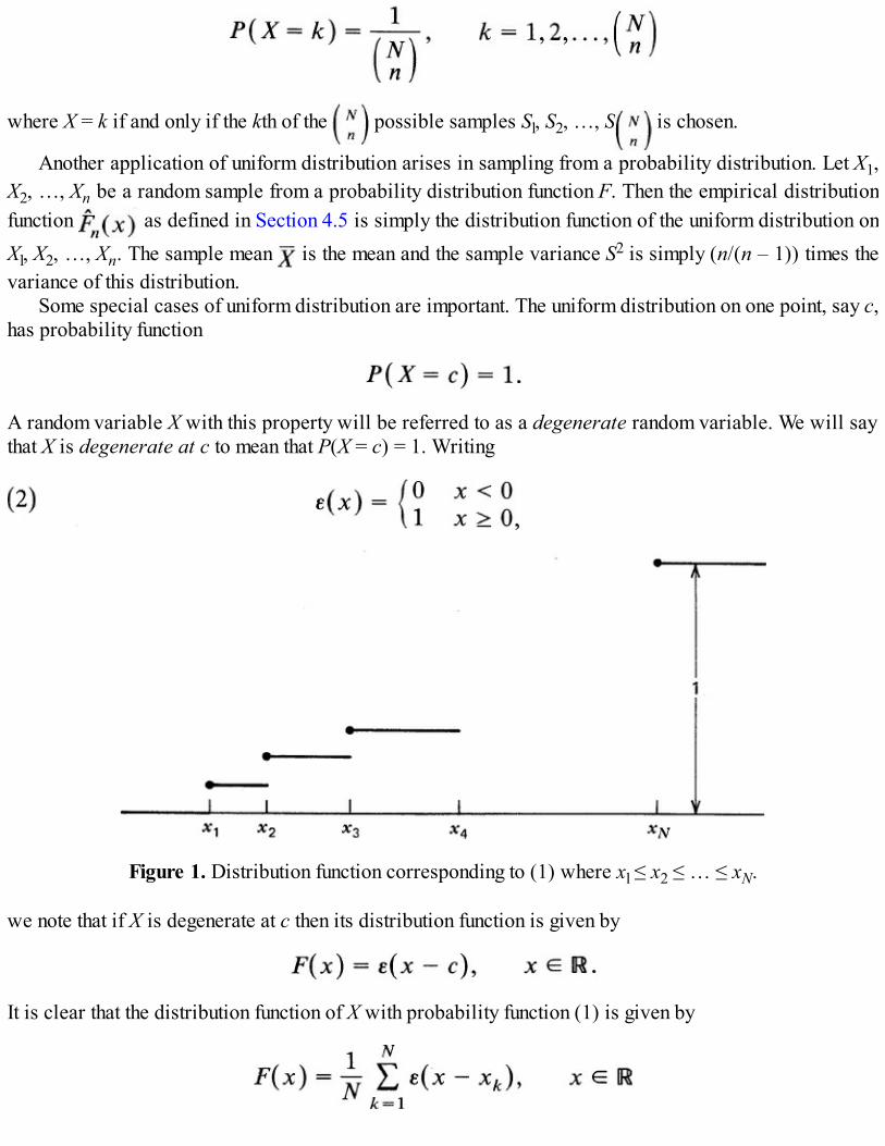
where X = k if and only if the kth of the possible samples Sl, S2, …, S is chosen.

Another application of uniform distribution arises in sampling from a probability distribution. Let X1,X2, …, Xn be a random sample from a probability distribution function F. Then the empirical distributionfunction as defined in Section 4.5 is simply the distribution function of the uniform distribution onXl, X2, …, Xn. The sample mean is the mean and the sample variance S2 is simply (n/(n – 1)) times thevariance of this distribution.

Some special cases of uniform distribution are important. The uniform distribution on one point, say c,has probability function

A random variable X with this property will be referred to as a degenerate random variable. We will saythat X is degenerate at c to mean that P(X = c) = 1. Writing

Figure 1. Distribution function corresponding to (1) where xl ≤ x2 ≤ … ≤ xN.

we note that if X is degenerate at c then its distribution function is given by

It is clear that the distribution function of X with probability function (1) is given by

which is a step function with graph as shown in Figure 1.Another special case of great interest is the N = 2 case with

which is discussed in greater generality and more detail in the next section.

Example 1. The Taxi Problem: Estimating the Number of Taxis in a Town. In Example 4.3.3 we considered the problem ofestimating N the number of taxis in a town (or the size of a finite population) on the basis of a single observation. We now consider theproblem of estimating N on the basis of a random sample of size n.

Consider an urn that contains N marbles numbered 1 through N. Suppose n marbles are drawn with replacement. Let Mn be thelargest number drawn. Then Mn is a random variable and can be used to estimate N. How good is this estimate? Clearly Mn ≤ N.Moreover,

since

by independence of the n draws. The mean of Mn is given by

Now

and for large N we can approximate it by the integral

Hence:

It follows that

so that is a nearly unbiased estimate of N for large N.Suppose that a town has N taxis numbered 1 through N. A person standing at a street comer notices the taxi numbers on n = 8 taxis

that pass by. Suppose these numbers (arranged in increasing order) are

An obvious estimate for N is = M8 = 926. Since N is large we can use the estimate

There are many other simple estimates of N that can be easily constructed.For example, the sample median is (628 + 684)/2 = 656. It follows that if we use the sample median to estimate the population median

we can use 2 = 656 + 655 = 1311 as an estimate of N. Yet another estimate can be obtained by noting that there are 123 taxis withnumbers smaller than the smallest observed number (= 124). Assuming that there are as many taxis with numbers larger than the largestobserved number we arrive at 3 = 926 + 123 = 1059 as an estimate of N. Which of these estimates do we choose? That depends onwhat we desire of our estimate. Do we want our estimate to be unbiased and have the least variance? Do we want our estimate to bewithin, say, 50 of the true N with 90 percent confidence? Some of these questions will be answered in general in Chapter 10 and inparticular in Example 10.3.4. See also Problems 3, 4, 7, 8, and 9 in the following problems section.

Problems for Section 6.2

1. Let X have uniform distribution on {1, 2, …, N}. Show that

(If you do not already know the sums of powers of the first N integers, use the following procedureto find them. Let . Then fs(1) = 1 = a1

Solve for a2, …, as+1 by substituting n = 2, 3, … successively. Show that: f1(n) = n(n + l)/2, f2(n) =n(n + 1)(2n + l)/6, f3(n) = [n(n + l)/2]2, f4(n) = n(n + 1)(2n + 1)(3n2 + 3n – l)/30.)

2. An urn contains N marbles numbered 1 through N. Two marbles are drawn one after the other asfollows. If the first marble is numbered k(k fixed, 1 ≤ k ≤ N), it is kept. Otherwise it is returned tothe urn. A second marble is then drawn. Find the probability that the second marble drawn isnumbered j(≠ k), 1 ≤ j ≤ N.

3. Consider the following procedure to estimate N in sampling from the uniform distribution on {1, 2,…, N}. Let xl, x2, …, xn be the n observed numbers in the sample of size n and assume, without loss

of generality, that x1 < x2 < ··· < xn.

Estimate the gaps between 1 to xl, x1 to x2,…, xn–1 to xn. Then estimate N by

Show that , where Mn is the largest observed number ( = xn here). ( 4 is

essentially N1 in Example 1.) The estimate 4 is called the gap estimate of N.4*. In Example 1 we assumed sampling with replacement in computing the distribution of Mn. (If N is

large then the probability that an observation appears twice is 1/N2 and is small. For large N,sampling with and without replacement are approximately the same.) Suppose N is not large andsampling is without replacement.(i) Show that:

and

(ii) Show that

Part (ii) shows that the gap estimate of Problem 3 is unbiased. [Hint: Use to

show that which may then be used to prove (ii).]

5. Consider a roulette wheel whose circumference is divided into 38 arcs, or sectors, of equal length.The sectors are numbered 00, 0, 1, …, 36. The wheel is spun and a ball is rolled on thecircumference. The ball comes to rest in one of the 38 sectors. Assume that the sector number sochosen has uniform distribution. Players betting $1 on any of the 38 numbers receive $36 if theirnumber shows up, and they lose their $1 if it does not. What is a player’s expected gain?

6*. A sample of size n is chosen without replacement from the finite population of N objects {x1, x2, …,

xN}. Show that the probability distribution of Xi the object selected on the ith draw, is uniform:

Also show that

(Thus, although Xi, Xj are not independent, their marginal distribution is uniform on xl, …, xN exactlyas in the case of sampling with replacement.)

7*. Let Xl, X2,…, Xn be a sample from the uniform distribution on {1, 2, … N}. Let Nn = min{Xl, X2, …,Xn}.(i) If Xl, X2, … , Xn are independent identically distributed (that is, if the sampling is with

replacement), find the distribution of Nn and find Nn. Find (Nn + Mn) and obtain an unbiasedestimate of N.

(ii) If the sampling is without replacement and Xj denotes the outcome of the jth draw, find thedistribution of Nn and Nn.

8. A random sample of five is taken from the uniform distribution on {1, 2, …, N}. The maximumobservation in the sample was 500. Is there evidence to doubt that N = 1500?

6.3 BERNOULLI AND BINOMIAL DISTRIBUTIONS

In a wide variety of random phenomena the outcome can be categorized into one of two mutuallyexclusive categories, usually but not necessarily referred to as success and failure. Such is the case, forexample, when a coin is tossed (heads success, tails failure), or when a dairy farmer observes the sex of anewly born calf (male, female), or when we observe the outcome of a delicate operation by a surgeon(successful or unsuccessful), and so on. Let Ω be a sample space and A ⊆ Ω be an event with P(A) = p, 0< p < 1. On Ω let us define a random variable X which is the indicator function of A, that is,

Then the probability function of X is given by

and we say that X is a Bernoulli random variable or that (1) is a Bernoulli probability function. Clearlythe distribution function of X is given by

and we see that

where ε(x) = 1 if x ≥ 0 and ε(x) = 0 if x < 0, as defined in equation (2) of Section 6.2. Moreover,

Any performance of an experiment that results in either a success or a failure is called a Bernoullitrial. Let us now consider the combined experiment consisting of n independent Bernoulli trials with aconstant probability p of success.

DEFINITION 1. An experiment with the following properties is called a binomial experiment:1. It consists of n trials.2. Each trial is dichotomous, that is, the outcome falls into one of two mutually exclusive categories: a success (S) or a failure (F).3. The probability of success P(S) = p remains constant from trial to trial.4. The trials are independent.

We shall be interested in the random variable

Example 1. Effectiveness of a Drug. A new drug that is effective in 30 percent of its applications is administered to 10 randomlychosen patients. What is the probability that it will be effective in five or more of these patients?

Let us check to see if this experiment meets the requirements of Definition 1.

(i) The experiment consists of n = 10 trials.(ii) The trials are dichotomous. Either the drug is effective (S) or ineffective (F) on a particular patient.(iii) The probability of success on each trial is .3.(iv) The trials are independent since the patients are randomly chosen.

It is therefore reasonable to conclude that this is a binomial experiment. Let X be the number of successes. Then we wish to find P(X ≥5). This computation will be made in Example 3.

Example 2. Probability of Successful Flight on a Jetliner. A jumbo jet has four engines that operate independently. Suppose thateach engine has a probability 0.002 of failure. If at least two operating engines are needed for a successful flight, what is the probability ofcompleting a flight?

Here the experiment consists of four trials that are dichotomous: either an engine is operating (S) or it has failed (F). Trials areindependent since the engines operate independently. Finally, p = P(S) = 1 – .002 = .998 is the same for each engine. If we let X =number of engines operating during the flight then

This computation is made in Example 4.

Let us now compute the probability function of X. Clearly P(0 ≤ X ≤ n) = 1. The sample spaceconsists of all n-length sequences of the letters S and F. Thus

and Ω has 2n outcomes. However, each sequence does not have the same probability (unless p = 1/2). Let0 ≤ k ≤ n be an integer. Then

Consider a typical sample point from the event (X = k). One such sample point is

Another is

and yet another is

In view of independence,

Similarly,

and

It is clear, therefore, that every sample point from (X = k) has the same probability, namely pk(1 – p)n–k,and we have

where summation is over those sample points having exactly k S’s and (n – k) F’s. It follows that

P(X = k) = (number of sample points with k S’s, (n – k) F’s) pk (1 – p)n – k.

Since the number of sample points with k S’s and (n – k) F’s is simply the number of ways of choosing kplaces for the S’s (and hence (n – k) places for the F’s), we have

Binomial Probability Function

Let us show that (4) does actually define a probability function. Indeed, P(X = k) ≥ 0 for every k and,moreover, by binomial theorem:

Since the Kth term in the binomial expansion [p + (1 – p)]n gives the probability of k successes, thedistribution defined by (4) is called a binomial distribution and X is called a binomial random variable.Given n and p we can compute any probability concerning X. Thus:

It is also useful to remember some frequently used terms: Term Event

Figure 1. Histogram for n = 10, p = .1, .5 and .8.

The distribution function of X is easy to compute. Indeed, for x ∈

Figure 1 shows the probability histograms of binomial probability functions for n = 10, p = .1, .5, .8.

Example 3. Effectiveness of a Drug (Continuation of Example 1). In Example 1 we had n = 10, p = .3 and we had to find P( X ≥5). From (4) we have

Example 4. Successful Flight on a Jetliner (Continuation of Example 2). In Example 2 we had n = 4, p = .998 and

A table of cumulative probability under binomial distribution frequently helps in computations. TableA3 in the Appendix gives the cumulative probabilities for some selected

values of n and p, and k = 0, 1, 2, …, n. For larger values of n one uses the normal approximationdiscussed in Chapter 9 (or the Poisson approximation, discussed in Section 6.6).

Cumulative probabilities for p > .5 can be extracted from Table A3 by the simple observation that

Thus if we want the probability of at most k successes in n trials with p > .5, then we look for theprobability of at least n – k failures each with probability (1 p)(< .5). Similarly,

The following relations are frequently useful:

Table A3 can also be used for finding values of k corresponding to a given probability in the tail ofthe distribution. Thus, given n and p we can find the smallest k such that

for a given α, 0 < α < 1, or the largest k such that

The following examples illustrate the use of Table A3.

Example 5. Effectiveness of a Drug. Experience has shown that with the present treatment, only 25 percent of all patients afflictedwith leukemia will be alive 10 years after the onset of the disease. A researcher has developed a new drug which is tried on 15 randomlyselected patients. It is found that 10 of these patients are still alive 10 years after the onset. Does the evidence indicate that the new drugis preferable to the present treatment?

The null hypothesis is H0: p = .25 to be tested against H1: p > .25. Let X be the number of patients in the sample of 25 who are still

alive 10 years after the onset. Then the P-value is

We conclude that the null hypothesis is not supported by the evidence.

Example 6. An Application to Quality Control A large lot of light bulbs is supposed to contain only 10 percent defectives. A sampleof size 25 is randomly selected from the lot and tested. How many defective bulbs should we observe in the sample before we concludethat the lot does not meet the specifications? Suppose the level of significance is α = .10.

Here n = 25 and H0: p = .10. Let X be the number of defectives in the sample. We wish to find the smallest k such that

Since Table A3 gives only P(X ≤ k), we rewrite this inequality as

From Table A3, the smallest k satisfying this inequality is given by k – 1 = 4, so that k = 5. If we observe five or more defective bulbs in asample of size 25, we should reject the lot and conclude that p > .1.

In the beginning of this section we assumed 0 < p < 1. Frequently we will include the (trivial) extremecases p = 0 and p = 1 and assume that 0 ≤ p ≤ 1.

Example 7. Estimating p. In practice p is unknown. To estimate p we note that the most probable value of k corresponds to thevalue of p given by

so that p = k /n. Since (d2/dp2)P(X = k) < 0, p = k /n is a maximum. Thus = k /n is that value of p which makes the outcome X = kmost probable. Therefore, = X/n is a reasonable estimate of p. Note that X/n is the proportion of successes in n trials and would havebeen the choice for estimating p on intuitive grounds. Further properties of this estimate are considered later.

In particular, if 10 successes are observed in 30 trials, then our estimate of p would be = 10/30 = 1/3.

Example 8. Reading Table A3 when p > .5. A random sample of 15 observations is taken from the density function

What is the probability that five of these observations will be smaller than .6? Note that n = 15 and p = P(Y < .6) where Y is a randomvariable with density f. Then p = .6. If X is the number of observations that are smaller than .6, then X has a binomial distribution with n =15 and p = .6. Since p > .5, we cannot directly read P(X = 5) from Table A3. But

Again,

and

6.3.1 Some Properties of Binomial Distribution

For later use, we will need some moments of the binomial distribution. We have

A simpler method to compute moments of X uses the binomial expansion:

Differentiating both sides of (7) with respect to x we get

and so on. Let us substitute x = p and y = 1 – p. We have

It follows that

and

Hence:

and

Mean and Variance of Binomial

It also follows that

where X/n is the proportion of successes in n trials.Next we note that the number of successes in n independent trials can be looked upon as the sum

where Xk = 1 if the kth trial results in a success, and Xk = 0 otherwise. Thus X is the sum of n independentand identically distributed Bernoulli random variables Xl,…, Xn, with Xk = p and var(Xk) = p(1 – p).

Similarly, if Yl, Y2 are two independent binomial random variables with parameters (nl, p) and (n2, p)the distribution of Yl + Y2 is also binomial (nl + n2, p) since we can look upon Yl + Y2 as the number ofsuccesses in n1 + n2 independent Bernoulli trials with probability of success p.

Returning to X/n, the proportion of successes in n trials, we note that it can be looked upon as asample average . Hence it must obey the weak law of large numbers studied inSection 5.4.

In fact, according to Chebyshev’s inequality, for every ε > 0

We note, however, that 4p(l – p) < 1 unless p = 1/2, in which case p(1 – p) = 1/4. [In fact, 4/p(l – p) – 1 =– (1 – 2p)2 < 0 for all p ≠ 1/2.] It follows that

Letting n → ∞ we see that

This special case of the weak law of large numbers (Section 5.4) is usually called the Bor el law of largenumbers.

The Borel Law of Large Numbers

Let A be any event. Then R(A), the relative frequency of A in n independent and identicaltrials of the experiment satisfies

as n → ∞. That is, as n increases, the probability that the relative frequency of A deviates fromP{A) by more than any given ε > 0 tends toward zero.

Remark 1. We emphasize once again that the law of large numbers as formulated here simply assertsthat for large n the relative frequency of A in n trials is likely to be close to P(A). It says that for every ε >

0, there is a sufficiently large n such that the probability that R(A) lies in the interval (p – ε, p + ε) can bemade as close to one as we wish. It does not assert the existence or the value of the limit for any particular sequence of trials in the ordinary sense of convergence of a sequence of real numbers. Itis true, however, that

but we will not attempt to prove this stronger result here.

Remark 2. Consider the special case when p = 1/2. Since X = n/2 and var(X) = n/4 we expect, onthe average, n/2 successes, and according to Chebyshev’s inequality, the number of successes will be inthe interval [(n – )/2,(n + )/2] with a probability of at least 8/9. For n = 100 this means thatP(35 ≤ X ≤ 65) ≥ 8/9. (This is a rather crude bound since the actual probability is .9991.) The law oflarge numbers does not say that in a large number of trials the number of successes and the number offailures will be approximately the same in the sense that their difference is near zero. The assertionconcerns only the proportion of successes (or failures). Thus in 100,000 tosses of a fair coin we mayobserve 51,000 heads and 49,000 tails. The proportion of heads and proportion of tails are nearly 1 /2and yet the difference between the number of heads and the number of tails is 2000. Similarly, it iscustomary to expect that in a coin-tossing game with a fair coin one player will lead the other roughly halfthe time. This is not true either.

Remark 3. The law of large numbers gives an estimate of the rate of convergence. It gives an upperbound for probability P(|X/n – p| ≥ ε) as 1/(4nε2), which is quite crude. A much more precise bound forthis probability is obtained by using the normal approximation (Section 9.4). If we take ε = .02, then

For n = 10,000, the upper bound is .06; for n = 100,000, the upper bound is .006.

Example 9. An Application to Opinion Polls . A pollster wishes to estimate the proportion of voters who favor the Equal RightsAmendment based on a random sample of size n. She wants to use the sample proportion of those who favor ERA as an estimate of thetrue proportion p. If the pollster wants the estimate to be within 3 percent of the true p, with probability ≥ .95, how large a sample shouldshe take?

The pollster wants to use X/n to estimate the unknown p such that

or,

Taking ε = .03 and 1/(4nε2) = .05 in (13) we get

The pollster should therefore take a sample of size at least 5556. At the expense of belaboring the point we emphasize that if the pollsterdoes take a sample of size 5556 and computes the relative frequency of respondents who favor ERA, then this number will either be

within 3% of the true p or not. Since p is unknown we will never know this for sure. The point is that if, say, 1000 samples were taken,each of size 5556, then for about 95 percent of these samples the relative frequency would be within 3 percent of the true p.

Example 10. Chebyshev’s Bounds for Proportion of Successes . Consider n tossings with a fair coin. Let X/n be the proportion ofsuccesses (heads). Clearly, (X/n) = 1/2 and var(X/n) = 1/(4n). By Chebyshev’s inequality

Let us choose k = 5 so that 1 – l/k2 = 24/25 = .96. Hence with a probability of at least .96, the proportion of successes will be between and .

n Bounds for Proportion of SuccessesMaximum Difference Between No. of

Successes of Successes and No. ofFailures

100 [.25, .75] 50625 [.4, .6] 12510,000 [.475, .525] 5001,0, 000 [.4975, .5025] 5000

6.3.2 Statistical Inference for the Binomial Distribution

In almost all our earlier discussions of the binomial distribution it was assumed that both p, theprobability of success, and n, the number of trials, are known. We have mostly concentrated on thecomputation of probabilities such as

either by direct computation or by the use of Table A3. That is, given n and p, the question we have so faranswered is this: Assuming that the binomial model conditions hold, what is the probability of observinga certain number of successes in n trials? We now reverse this process and ask questions concerning pbased on an observed number of successes. For example, if we observe five heads in 100 tosses of acoin, we ask what is a reasonable estimate of p? Can conclude that the coin is fair?

We first consider the point estimation of p. Suppose in n independent and identical Bernoulli trialswith P(success) = p we observe X successes. Suppose further that p is unknown. Consider the statistic

We note that 0 ≤ ≤ 1 so that is an estimate of p; it maps the sample space into the parameter set Θ =[0,1]. Moreover:

(i) is unbiased.(ii) P( – p| ≥ ε) → 0 as n → ∞ so that is consistent for p. The probability that will deviate from p

by more than any fixed amount ε > 0 can be made as small as we please by taking n sufficiently

large.(iii) = k/n maximizes P(X = k).(iv) var( ) = p(1 – p)/n; the variance of can be made as close to 0 as we please by taking n

sufficiently large.

Thus is a reasonable point estimate of p. Some other properties of will be considered later. Note,however, that is a statistic (random variable); its value varies from sample to sample. The probabilitythat equals p is usually small. Indeed,

is zero when np is not an integer. Even when np is an integer this probability is small. For n = 20, p = .4,

and for n = 100, p = .5

The estimate , therefore, and any other point estimate of p for that matter, is of limited value. In manyapplications what we want are bounds that will include the unknown value of p with a large probability.In other words, we want a confidence interval for p.

Let 0 < α < 1. Then we wish to find random variables l(X) and u(X) such that

Since X is a discrete type random variable, minimum level 1 – α confidence intervals [l(X), u(X)] do notexist for all α. We therefore replace the equality sign in (14) by “≥” and seek confidence intervals for p atlevel at least 1 – α. (See Section 4.3.) By Chebyshev’s inequality we have for ε > 0

Since p(1 – p) ≤ we have

Rewriting (16), we have

Let us now compare (14) and (17). We have

so that and

Point and Interval Estimates for p

The proportion of successes = X/n is a good point estimate for p.

The interval is a 100(1 – α) percent confidence interval for p.

Example 11. Busing to Achieve Racial Balance . Of 100 people interviewed, 79 registered opposition to busing students to achieveracial balance. Let p be the true proportion in the population of those who oppose busing. Then a point estimate of p based on this sampleof size n = 100 is given by

so (we estimate) that more than half the population is not in favor of busing. Suppose that the true p is .5. What is the probability ofobserving ≤ .79 in a sample of size 100 in random sampling from a population where in fact p = .5? We have

from Table A3 with n = 100 and p = .5. It is therefore reasonable to conclude the true proportion of those opposed to busing in thispopulation exceeds .5.

Suppose, instead, that we want a 95 percent confidence interval for p. Then 1 – α = .95, α = .05, and a 95 percent confidence intervalis given by

(the largest value of p is 1). This confidence interval has width .43. It is clear that the sample size is too small (and the interval is toocrudely constructed) to give a narrow width. We note, however, that p = .5 is not included in this interval.

Example 12. An Improved Confidence Interval for p . The interval [ – , ] is a somewhat crudeconfidence interval for p. The length of a confidence interval is taken as a measure of its accuracy. The smaller the length the moreinformative is the confidence interval. The length of the above confidence interval is given by

which does not even depend on the observations. This feature, however, allows us to choose the sample size to guarantee a fixed lengthof d (> 0), say. In fact, by choosing

the confidence interval will be a 100(1 – α)% confidence interval with width at most d.

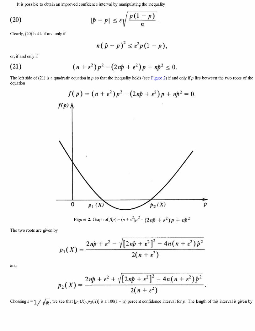
It is possible to obtain an improved confidence interval by manipulating the inequality

Clearly, (20) holds if and only if

or, if and only if

The left side of (21) is a quadratic equation in p so that the inequality holds (see Figure 2) if and only if p lies between the two roots of theequation

Figure 2. Graph of f(p) = (n + ε2)p2 –

The two roots are given by

and

Chossing ε = , we see that [p1(X), p2(X)] is a 100(1 – α) percent confidence interval for p. The length of this interval is given by

which is a random variable. Therefore we cannot compare L1 and L2 directly. if n is large, however, then we can by p in theexpression for L2. In that case:

Thus, at least for large n, the 100(1 – α) percent confidence interval [p1(X) , p2(X)] should be narrow than the 100(1 – α) percentconfidence interval given in (18).

Returning to the data of Example 11 for comparison purposes, we see that with n = 100, = .79, α = .05,

so that

Thus a 95 percent confidence interval is [.5685, .9149]. This confidence interval has width 2(.1732) = .3464, which is much smaller thanthe width of the confidence interval considered in Example 11. In this sense, it is an improved confidence interval.

We note that the confidence intervals considered here are generally applicable and are used for smallor moderate sample sizes. As we shall see, for large samples we can do much better.

Finally, we consider the problem of testing hypotheses concerning p. The methods of this section areexact and apply to the case when n is small or moderate.

Example 13. Change of Voting Preference . Congressional District 5 in Wood County has consistently voted 60 per cent or moreRepublican in the past 20 years in Congressional elections. It is suspected that the depressed economic conditions during 1981—82 mayhave changed the percentage of voters who will vote for the Republican candidate for Congress in 1982. In a random sample of 25 votersfrom this district 12 voters indicated that they plan to vote Republican. Have the depressed economic conditions changed votingpreference?

Here the null hypothesis to be tested is H0: p ≥ .60 where p = true proportion of voters in the district who plan to vote Republican.This is a one-sided hypothesis to be tested against the alternative that H1. p < .60. Let X be the number of voters in the sample who favorRepublicans. Since X = 12 is observed, our estimate of p is = 12/25 = .48, which is less than .60. The question is, How probable is sucha small value of in random sampling from a population where p ≥ .60? In other words, we seek the probability

However, this cannot be done unless p is completely specified. We note that

since if p > .60 we would expect more successes (that is more voters in favor of the Republican candidate). Now

Thus, unless the level of significance α is at least .154 we have to conclude that there is not enough evidence to support the rejectionof H0. If we reject H0 when X is at most 12, what is the probability of a type II error? This depends on the true p. Suppose p = .5. Thenthe probability of a Type II error is given by

The smaller the p the smaller this error. The power at p = .5 is 1 – P (type II error) = .5.Given α, 0 < α < 1, the level of significance, how do we find the critical region of a level α test of H0 : p ≥ .60 against H1: p < .60?

Since larger values of X support H0, a reasonable critical region is given by {X ≤ c} where c is the largest integer satisfying

Since, as pointed out above,

it suffices to choose the largest c satisfying

The values of c for some selected values of α are given below.

The probability of a type II error if we choose α = .05 say, so that c = 10, is given by PHl(X ≥ 11). For some selected values of p(< .60),the type II error probabilities are given below.

The procedure for testing H0: p ≤ p0 against H1: p > p0 or for testing p = p0 against p ≠ p0 is similar.We summarize the results below.

Testing Binomial p

Let X have a binomial distribution with parameters n and p and suppose that X = x0 is theobserved number of successes.

In the case when H0: p = p0 is to be tested against H1. p ≠ p0 we have used the conventional equal-tails approach. Thus, if the level of significance a is given, we distribute it equally in the two tails tocompute the critical values c1 and c2. If α is not given and we decide to reject with probability P{X ≤ x0/p= p0] in the left tail, presumably we will allow the same probability of error in the right tail. The criticalvalue in the right tail is computed by taking the smallest c such that

In the special case when p0 = , c = n – x0.

Example 14. Sex Ratio of Births at a Hospital. It is desired to test that the sex ratio of births at a hospital is .5. A random sampleof 20 births showed 13 girls. Let X be the number of female births in the sample and let p be the probability that the sex of a newly bornchild is female. Then we wish to test H0: p = p0 = .5 against H1: p ≠ .5. Here x0 = 13 so the smaller tail probability is given by:

The P-value is 2(.132) = .264, and there is not enough evidence to reject H0. To find the corresponding rejection region in the left tailwe choose the largest c such that:

From Table A3, c = 7. (Since p0 = .5, c = n – x0 = 20 – 13 = 7.) The size .264 rejection region then is {0, 1, …, 7, 13, 14, …, 20}.On the other hand, if we are given the level of significance α = .10, say, we reject H0 if the observed x0 ∈ {0, 1, …, c, n – c, n – c +

1, …, n} where c is chosen from (the largest value)

From Table A3, c = 5 so that the rejection region is {0, 1, 2, 3, 4, 5, 15, 16, 17, 18, 19, 20}. The size of the corresponding test is 2(.021) =.042. Since x0 = 13 does not fall into this region, we cannot reject H0 at level .10.

6.3.3 An Application of Binomial Distribution: Sign Test

Suppose a new diet is designed to lower cholesterol levels. How do we go about testing whether the dietis effective or not? One way to do so would be to take a random sample of n subjects and put them on thisdiet for, say, six months. Let Xi be the cholesterol level of the ith subject before he or she goes on the diet,and let Yi be his or her cholesterol level after six months. If the diet is effective on the ith subject, Xi – Yiwill be positive. The number of pairs (Xi, Yi) for which Xi – Yi > 0 is then a measure of the effectiveness

of the diet. The larger this number, the more plausible it is that the diet is effective. The null hypothesisthat we wish to test is

against the alternative

We will assume in the following that (X, Y) is jointly of the continuous type so that P(X = y) = 0, that is,ties occur with zero probability. In that case, under H0

or

and under H1.

Let S be the number of pairs for which Xi < Yi. Then S has a binomial distribution with parameters n and p= P(X < Y) where p ≥ under H0. The test (for small samples) that we use is the one-sided test describedin Section 6.3.2. We reject H0 if S is small (or equivalently, the number of pairs with Xi – Yi > 0 large),that is,

If α is known we choose the largest c such that

A similar procedure applies for testing p ≤ or p = . Since the test statistics counts the number ofnegative (or positive) signs Xl – Y1, X2 – Y2,…, Xn – Yn, the resulting test is called a sign test.

The Sign Test

To test for jointly continuous type random variables X and Y, the null hypothesis

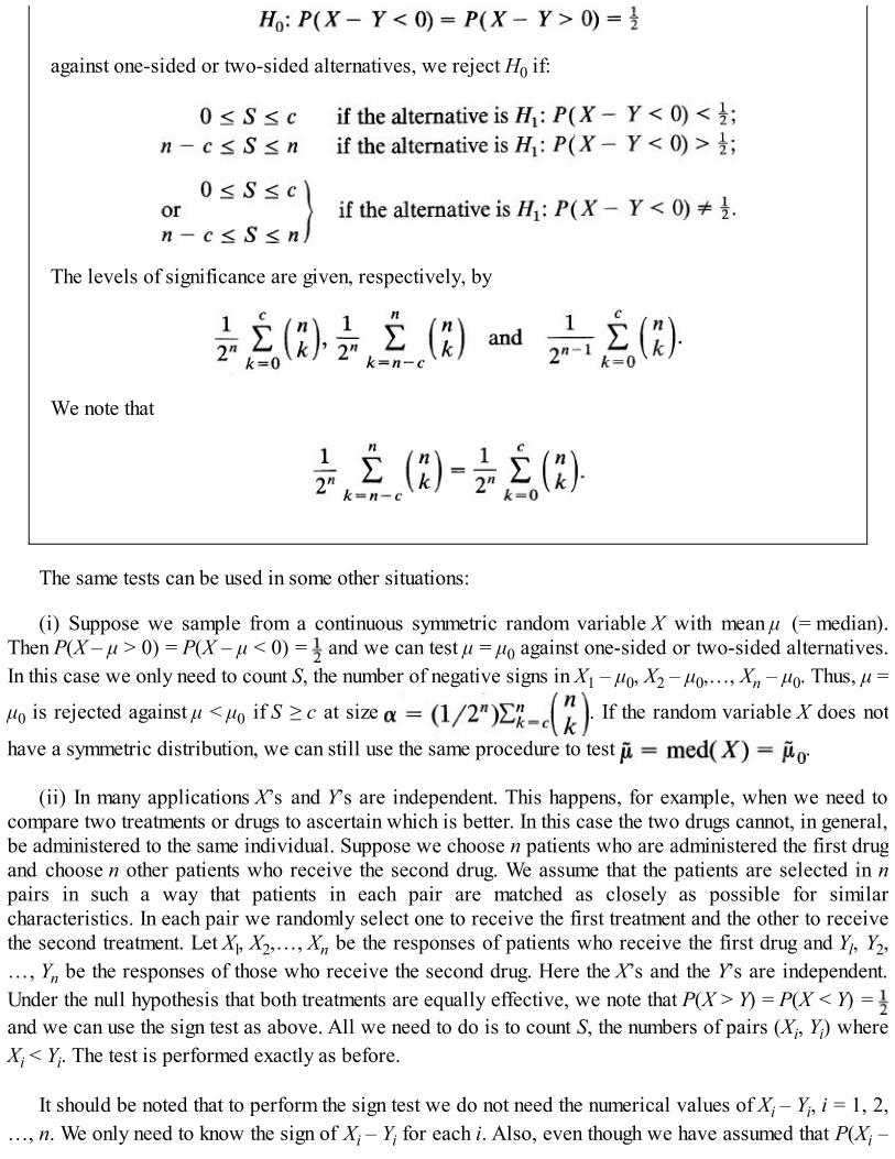
against one-sided or two-sided alternatives, we reject H0 if:

The levels of significance are given, respectively, by

We note that

The same tests can be used in some other situations:

(i) Suppose we sample from a continuous symmetric random variable X with mean μ (= median).Then P(X – μ > 0) = P(X – μ < 0) = and we can test μ = μ0 against one-sided or two-sided alternatives.In this case we only need to count S, the number of negative signs in X1 – μ0, X2 – μ0,…, Xn – μ0. Thus, μ =

μ0 is rejected against μ < μ0 if S ≥ c at size . If the random variable X does not

have a symmetric distribution, we can still use the same procedure to test .

(ii) In many applications X’s and Y’s are independent. This happens, for example, when we need tocompare two treatments or drugs to ascertain which is better. In this case the two drugs cannot, in general,be administered to the same individual. Suppose we choose n patients who are administered the first drugand choose n other patients who receive the second drug. We assume that the patients are selected in npairs in such a way that patients in each pair are matched as closely as possible for similarcharacteristics. In each pair we randomly select one to receive the first treatment and the other to receivethe second treatment. Let Xl, X2,…, Xn be the responses of patients who receive the first drug and Yl, Y2,…, Yn be the responses of those who receive the second drug. Here the X’s and the Y’s are independent.Under the null hypothesis that both treatments are equally effective, we note that P(X > Y) = P(X < Y) = and we can use the sign test as above. All we need to do is to count S, the numbers of pairs (Xi, Yi) whereXi < Yi. The test is performed exactly as before.

It should be noted that to perform the sign test we do not need the numerical values of Xi – Yi, i = 1, 2,…, n. We only need to know the sign of Xi – Yi for each i. Also, even though we have assumed that P(Xi –

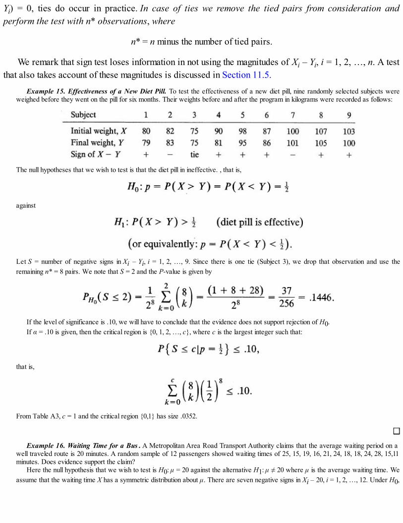
Yi) = 0, ties do occur in practice. In case of ties we remove the tied pairs from consideration andperform the test with n* observations, where

n* = n minus the number of tied pairs.

We remark that sign test loses information in not using the magnitudes of Xi – Yi, i = 1, 2, …, n. A testthat also takes account of these magnitudes is discussed in Section 11.5.

Example 15. Effectiveness of a New Diet Pill. To test the effectiveness of a new diet pill, nine randomly selected subjects wereweighed before they went on the pill for six months. Their weights before and after the program in kilograms were recorded as follows:

The null hypotheses that we wish to test is that the diet pill in ineffective. , that is,

against

Let S = number of negative signs in Xi – Yi, i = 1, 2, …, 9. Since there is one tie (Subject 3), we drop that observation and use theremaining n* = 8 pairs. We note that S = 2 and the P-value is given by

If the level of significance is .10, we will have to conclude that the evidence does not support rejection of H0.If α = .10 is given, then the critical region is {0, 1, 2, …, c}, where c is the largest integer such that:

that is,

From Table A3, c = 1 and the critical region {0,1} has size .0352.

Example 16. Waiting Time for a Bus . A Metropolitan Area Road Transport Authority claims that the average waiting period on awell traveled route is 20 minutes. A random sample of 12 passengers showed waiting times of 25, 15, 19, 16, 21, 24, 18, 18, 24, 28, 15,11minutes. Does evidence support the claim?

Here the null hypothesis that we wish to test is H0: μ = 20 against the alternative H1: μ ≠ 20 where μ is the average waiting time. Weassume that the waiting time X has a symmetric distribution about μ. There are seven negative signs in Xi – 20, i = 1, 2, …, 12. Under H0,

The P-value, therefore, is 2(.3871) = .7742 and there is hardly any evidence to reject the claim.If, on the other hand, α is given to be, say, .10, then the rejection region is (0, 1, …, c, 12 – c,…, 12}, where c is the largest integer

such that

It follows that c = 2. The rejection region {0, 1, 2, 10, 11, 12} has size 2(.0193) = .0386. Since S = 7 is not in the critical region, we cannotreject H0 at a 10 percent level of significance.

Problems for Section 6.3

1. In each of the following cases, state whether the random variable X can or cannot be assumed tohave a binomial distribution. Give reasons for your answer.(i) In a statistics class of 25 students, four are selected at random. Let X be the number of seniors in

the sample.(ii) About 5 percent of students registered for a statistics course are absent from the first class in

Winter semester (which starts in mid-January) because they have colds. Let X be the number ofstudents with colds who will be absent from the first class in this statistics course in the comingWinter semester out of a total of 35 in the course.

(iii) Let X be the number of babies having blonde hair out of 20 (independent) births at the countyhospital.

(iv) Let X be the number of patients cured of a certain infection out of 15 who were treated withpenicillin.

(v) Twenty-five people were asked to try two different brands of detergent. Let X be the number ofthose who prefer Brand A over Brand B.

(vi) A random sample of 50 persons from a large population is asked the question, Do you smoke?Let X be the number of those who smoke.

2. A well-known baseball player has a lifetime batting average of .300. If he comes to bat five times ina game, find the probability that:(i) He will get at least one hit.(ii) He will get more than three hits.(iii) He will get no hits.

3. About 10 percent of mail solicitations result in a donation. Find the probability that of a randomlyselected 20 people who receive a mail solicitation five or more will donate some money.

4. From past experience it is known that about 90 percent of all stolen cars are recovered. Find theprobability that at least six of 10 stolen cars will be recovered.

5. A binomial random variable X has mean μ and variance a2.(i) Find the distribution of X. In particular, let μ, = 10 and σ2 = 6. Find P(X ≥ 10).(ii) Do μ = 5, σ2 = 4 and μ = 5, σ2 = 6 define binomial random variables?

6. For n = 25 and p = .3 and p = .8, use Table A3 to find:(i) P(X > 4). (ii) P(5 < X < 9). (iii) P(X ≤ 6).(iv) P(4 < X ≤ 8).

7. For p = .2 and n = 25, use Table A3 to find:

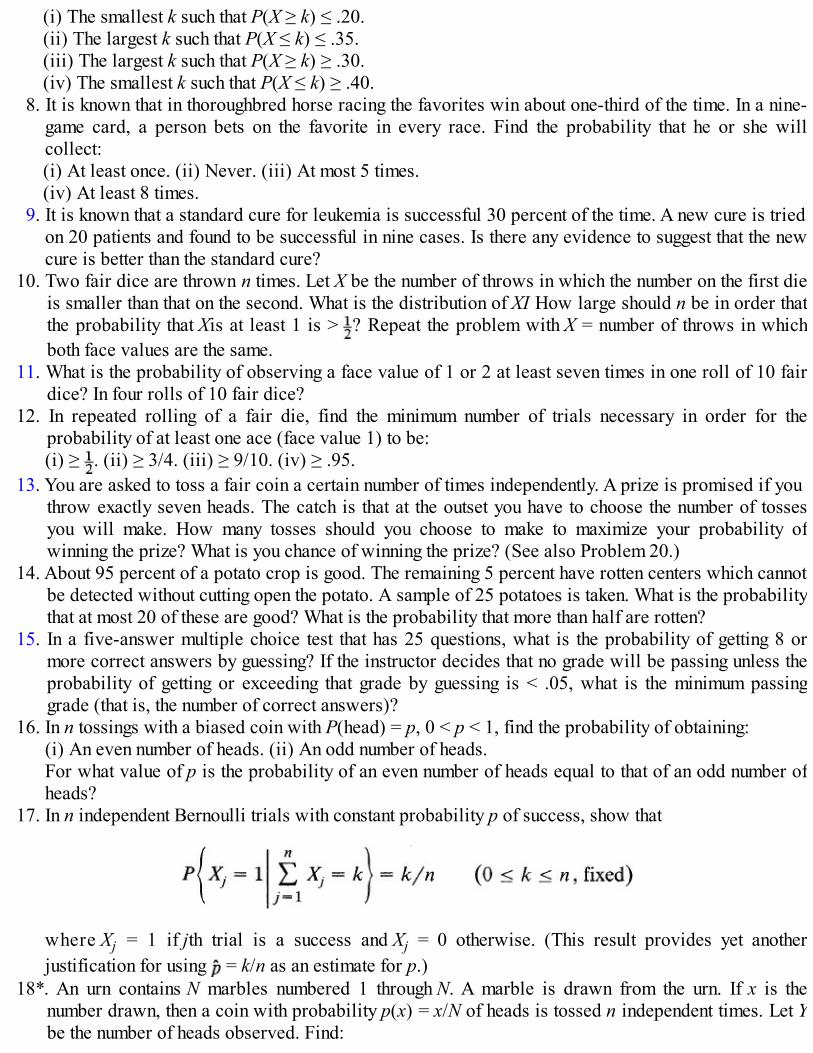
(i) The smallest k such that P(X ≥ k) ≤ .20.(ii) The largest k such that P(X ≤ k) ≤ .35.(iii) The largest k such that P(X ≥ k) ≥ .30.(iv) The smallest k such that P(X ≤ k) ≥ .40.

8. It is known that in thoroughbred horse racing the favorites win about one-third of the time. In a nine-game card, a person bets on the favorite in every race. Find the probability that he or she willcollect:(i) At least once. (ii) Never. (iii) At most 5 times.(iv) At least 8 times.

9. It is known that a standard cure for leukemia is successful 30 percent of the time. A new cure is triedon 20 patients and found to be successful in nine cases. Is there any evidence to suggest that the newcure is better than the standard cure?

10. Two fair dice are thrown n times. Let X be the number of throws in which the number on the first dieis smaller than that on the second. What is the distribution of XI How large should n be in order thatthe probability that Xis at least 1 is > ? Repeat the problem with X = number of throws in whichboth face values are the same.

11. What is the probability of observing a face value of 1 or 2 at least seven times in one roll of 10 fairdice? In four rolls of 10 fair dice?

12. In repeated rolling of a fair die, find the minimum number of trials necessary in order for theprobability of at least one ace (face value 1) to be:(i) ≥ . (ii) ≥ 3/4. (iii) ≥ 9/10. (iv) ≥ .95.

13. You are asked to toss a fair coin a certain number of times independently. A prize is promised if youthrow exactly seven heads. The catch is that at the outset you have to choose the number of tossesyou will make. How many tosses should you choose to make to maximize your probability ofwinning the prize? What is you chance of winning the prize? (See also Problem 20.)

14. About 95 percent of a potato crop is good. The remaining 5 percent have rotten centers which cannotbe detected without cutting open the potato. A sample of 25 potatoes is taken. What is the probabilitythat at most 20 of these are good? What is the probability that more than half are rotten?

15. In a five-answer multiple choice test that has 25 questions, what is the probability of getting 8 ormore correct answers by guessing? If the instructor decides that no grade will be passing unless theprobability of getting or exceeding that grade by guessing is < .05, what is the minimum passinggrade (that is, the number of correct answers)?

16. In n tossings with a biased coin with P(head) = p, 0 < p < 1, find the probability of obtaining:(i) An even number of heads. (ii) An odd number of heads.For what value of p is the probability of an even number of heads equal to that of an odd number ofheads?

17. In n independent Bernoulli trials with constant probability p of success, show that

where Xj = 1 if jth trial is a success and Xj = 0 otherwise. (This result provides yet anotherjustification for using = k/n as an estimate for p.)

18*. An urn contains N marbles numbered 1 through N. A marble is drawn from the urn. If x is thenumber drawn, then a coin with probability p(x) = x/N of heads is tossed n independent times. Let Ybe the number of heads observed. Find:

(i) P{Y = k}, for k = 0, 1, …, n. (ii) Y.(iii) P{X = x\Y = k] where X denotes the number on the marble drawn.

19*. Let X be the number of successes and Y the number of failures in n independent Bernoulli trials withP(success) = p. Let U = X – Y. Show that the distribution of U is given by:

where k = –n, 2 – n, 4 – n,…, n – 4, n – 2, n. Moreover,

and for ε > 0

20*. For the binomial distribution, show that the most probable number of successes (for given p and n)is k where

unless P(X = k – 1) = P(X = k), in which case k = (n + 1)p. [Hint: Show that

so that P(X = k) > P(X = k – 1) if and only if k < (n + 1)p. This result can be used to estimate n forgiven p and is not inconsistent with Example 7.]

21*. Let X be the number of successes in n independent Bernoulli trials, each with a constant probabilityof success equal to p, 0 < p < 1. Then X has a binomial distribution. Derive the probability functionof X as follows. Let f(n, k) = P(X = k).(i) Show that

(Hint: The last trial is either a success or a failure.)(ii) Show by induction that

For k = 0, f(n, 0) = (1 – p)n by direct computation and for k = n, f(n, k) = pn by direct computation.Clearly f(n, k) = 0 for k > n. Take f(0, 0) = 1.

[Hint: for 1 ≤ r ≤ n – 1.]

(iii) Let X = h(n). Use the result in part (i) to deduce that

with h (0) = 0. Conclude, by summing, that

[Hint: ](iv) Let X(X – 1) = g(n). Use the result in part (i) to show that

with g(0) = 0, g(l) = 0. Hence show that g(n) = n(n – 1)p2, n = 2, 3, … and deduce that var(X) =np(1 – p). [Hint: .]

22*. Show that for a binomial random variable X

(Hint: Integrate by parts. Alternatively, differentiate both sides with respect to p, simplify the rightside, and then integrate. This formula gives a method of computing the distribution function of X interms of an incomplete beta function. See Chapter 7, Sections 7.3 and 7.5.)

23*. If k ≥ np, show that the probability function of a binomial random variable satisfies

and if k ≤ np, then

[Hint: P(X = k)/P(X = k – 1) = p(n + 1 – k)/k(l – p) < 1 if and only if k > (n + 1)p. Hence the ratiodecreases monotonically as k increases. Conclude that

and hence that

Sum over v = 0 to n – r, noting that this sum is bounded by the sum of an infinite geometric series.]24*. Let N be a binomial random variable with parameters q, 0 < q < 1, and M. Let the conditional

distribution of X, given N = n, be binomial with parameters p and n. Find the unconditionaldistribution of X and its mean and variance.

25*. As an application of Problem 24, let N1 be the (random) number of contacts that an insurance

salesman makes. Suppose N = N1 – 1 is binomial with parameters M – 1 and q, 0 < q < 1. Let X bethe number of sales that result. Suppose the conditional distribution of X given N1 = n is binomialwith parameters n and p. Find the unconditional distribution of X, its mean and its variance. If eachsale results in a commission of $C, find the expected commission and its variance.

26. A venire is an order by a judge to a sheriff instructing him to summon persons to serve as jurors; aperson called to jury duty on such an order is called a venireman. Find the probability of at mostfive nonwhites in a venire of 25 when the probability of selecting a single nonwhite is p. Computethis probability for p = .20, .15, .10, and .05. In each case find the probability of selecting 20 suchvenires independently. Comment on your results.

27. A random sample of 20 students at a large state university was asked to respond to the question “Doyou favor conversion to a semester system?” There were 13 Yeses and 7 Noes.(i) Estimate p, the true proportion of students who favor conversion.(ii) If the students were evenly divided on this question, what is the probability of observing as many

as 13 Yeses in the sample?(iii) What is the mean and variance of your estimator of p in part (i) if the true proportion of Yeses

is .6?(iv) Find P{ – p| ≤ .l|p = .6}, the probability that your estimate will be within .1 of the true value

p = .6.(v) Find Chebyshev’s inequality upper bound for P(| – p| ≥ .1).(vi) Find a 90 percent confidence interval for p based on Chebyshev’s inequality. Also compute the

improved 90 percent confidence interval for p. Compare the lengths of the two intervals.28. A manufacturer of missiles wishes to estimate the success rate of its missiles. A random sample of

18 missiles was fired, and 16 firings were classified as successful. If the manufacturer wishes toestimate the true success rate p of its missiles by , the observed proportion of successes, what ishis estimate?

Find a 95 percent confidence interval for p based on Chebyshev’s inequality. Also find theimproved 95 percent confidence interval for p.

Suppose he wishes to estimate p by p to within .02 with 95 percent confidence, how manymissiles need he test-fire?

29. A major soft drink company wishes to estimate the proportion of shoppers who can identify a newsoft drink introduced by the company in order to assess the success of its advertising campaign. In arandom sample of 25 shoppers, only 10 were able to identify the soft drink.(i) What estimate of p, the true proportion of shoppers who can identify the drink, should it use?(ii) What is the probability of observing as small a proportion as the one observed if the true p is

.50?(iii) Find a 95 percent confidence interval for p.(iv) If the company wishes to estimate p by to within .05 with 90 percent confidence, how large a

sample should it take?(v) Find P{| – p| ≤ .2|p = .5}.

30*. A survey of students at a junior high school is conducted to determine the percentage of those whosmoke regularly. A random sample of 25 students showed that 10 smoked regularly.(i) If you estimate the true proportion of smokers by the sample proportion , find P{ ≤ 4|p = .5}.(ii) Find P{| – p| ≤ l|p = .5}.(iii) Find a 90 percent confidence interval for the true p.(iv) If you wish to estimate p to within .02 with 95 percent confidence, how large a sample size must

be taken?

31. A random sample of 100 people showed that 40 believe in UFO’s. Find a 95 percent confidenceinterval for the true proportion of the population which believes in UFO’s.

32. A coin is tossed 15 times and four heads are observed.(i) Is there evidence to suggest that the coin is biased in favor of tails? What is the P-value of your

test if you were to reject H0: p = 1/2? (Here p = probability of a head.)(ii) Take α = .05. Find the critical region for testing H0 at level α = .05. What is the size of this

critical region?(iii) Find the power of the test in (ii) at p = .4, p = .3, p = .2, p = .1.

33. A random sample of 20 faculty members from the faculty of a large state university showed that eighthad published during the last five years. Is it reasonable to assert that about half the faculty at thisuniversity has published during the last five years?

What will be your conclusion if the level of significance α = .10? Find the power of your level.10 critical region at p = .3, .4 and p = .6, .7.

34. In a random sample of 100 people, 25 had blue eyes. Does the evidence support the claim that theproportion of blue-eyed people is > .20? Find the critical region of a level .05 test.

Find the power of this critical region at p = .3, .4, and .5.35. It is estimated that 25 percent of all automobiles in a certain state do not meet minimum safety

standards. The State Auto Safety Council launched a six-month advertising campaign to encouragemotorists to have their autos checked. In order to check the effectiveness of its campaign, the councilexamined a random sample of 100 cars and found that 18 did not meet the minimum safety standards.Is there evidence to suggest that the campaign has had some effect?

What will your conclusion be if α = .1?36. A well-known seed company claims that 80 percent of its coriander seeds germinate. A random

sample of 100 seeds is planted and 25 fail to germinate. Is there evidence that the company’s claimis false? Find the critical region of your test if α is given to be .08. Find the power of your test at p =.7, p = .6, and p = .5.

37. Find the critical region of a level α test in each of the following cases:(i) H0: p = .10 against H1: p > .10 with n = 25, α = .05.(ii) H0: p = .30 against H1: p ≠ .30 with n = 20, α = .10.(iii) H0: p = .30 against H1: p < .30 with n = 20, α = .10.(iv) H0: p = .25 against H1: p ≠ .25 with n — 100, α = .14.

38. A manufacturer of light bulbs claims that 90 percent of its bulbs have a life length of 2000 hours ormore. A consumer takes a sample of size 15 and decides to reject the manufacturer’s claim if hefinds two or more bulbs in the sample that fail before 2000 hours.(i) What is the size of the test?(ii) Find the probability of a type II error if the true proportion of defectives is .20. Repeat for p =.30, p = .40, p = .50.

39. It is claimed that 25 percent of the marbles in an urn are numbered 50 or less. A random sample of100 marbles (drawn with replacement) from the urn produced only 10 marbles numbered 50 or less.Do you have any reason to doubt the claim? At what level of significance would you reject theclaim?

40. A panel of 12 wine tasters A, B, …, L was asked to test two varieties of wine: Cabernet Sauvignonand Pinot Noir. Each member of the panel ranks the two wines according to his or her preference.Rank 2 is more preferred than rank 1. The following rankings were awarded.

(i) Is there evidence to suggest that the two varieties are equally preferred?(ii) If a significance level of α = .10 is given, what is the critical region of your test for testing H0: p

= 1/2 against H1 : p ≠ 1/2? What is the size of your critical region? (Here p = P (CabernetSauvignon preferred over Pinot Noir).)

41. Ten chickens are fed an experimental diet for four weeks and their weight gains in ounces arerecorded as follows:

It is claimed that the median weight gained is 48 ounces. Test the claim at α = .10 level ofsignificance.

42. Thirteen randomly selected volunteers A, B,…, M are administered a pill designed to lower systolicblood pressure with the following results.

(i) Is there evidence to suggest that the pill is not effective?(ii) If a significance level of α = .15 is given, find the critical region of your test.

43. A course is taught by two methods: the classroom instruction method A and the self-study method B.Ten students each are selected randomly and carefully matched according to their background andability prior to instruction. At the end of the course the 10 pairs of scores are recorded as follows:

Do the data indicate any significant difference between the two methods at 10 percent level?44. Eleven students are given a course designed to improve their I.Q. on a standard test. Their scores

before and after the course are recorded as follows:

What can you conclude about the effectiveness of the course?45. Twenty-five drivers are randomly selected and tested for reaction times. After three alcoholic

drinks, the same test is administered. It is found that 18 had slower reaction times, 5 drivers

registered no change, and 2 had faster reaction times. Is there evidence to suggest that the reactiontimes remain unaffected due to drinking?

46. Given p, how will you estimate n based on the number of successes X?47. Two proofreaders independently read a manuscript and find X1, X2 typographical errors. Let X12 be

the number of errors found by both proofreaders. How will you estimate the total number of errors inthis manuscript? (Hint: Use the law of large numbers.)

6.4 HYPERGEOMETRIC DISTRIBUTION

In estimating the size of an animal population, the following capture-recapture procedure is frequentlyused. A sample of size D is captured, tagged, and then released into the population. After awhile a newcatch of n animals is made, and the number of tagged animals in the sample is noted. Let X be this number.Assuming that the two catches can be considered as random samples from the population of all animals,Xis a random variable and provides an estimate of the total population of animals. Indeed, if we assumethat there were no births or deaths, then we expect the proportion of tagged animals in the sample to beapproximately the same as that in the population. If N is the true size of the animal population then

so that an estimate of N is = nD/X. We will see later that this estimate maximizes the probability of theobserved value of X.

The distribution of X is called a hypergeometric distribution. Let us compute the probability functionof X. Figure 1 shows the sampling scheme. First note that there are samples of size n each of which

is assigned the same probability, l/ . To find P(X = k) we need only count the number of samples

containing exactly k tagged animals [and hence (n – k) untagged animals]. Since the k tagged animals mustbe chosen from D and (n – k) untagged animals from

Figure 1. Sampling scheme.

(N – D) the number of such samples (by Rules 1 and 3 of Section 2.5). It follows that

Note that

so that.

Hypergeometric Probability Function

where k = max(0, n + D – N),…, min(D, n).

Let us verify that (1) is indeed a probability function. Clearly, P(X = k) ≥ 0 since the binomialcoefficients are all ≥ 0. We need the following identity:

where we have used the convention that = 0 whenever k > a; a, b and m are positive integers.Consider the identity

The coefficients of x on both sides must be the same (why?). Equating the coefficients of xm on both sidesof (3), using binomial expansions, we get (2). We take a = D, b = N – D, and m = n in (2) to get

so that . [Again we have used the convention that = 0 whenever a < k.] Hence(1) defines a probability function.

Hypergeometric distribution arises in many practical problems where the population being sampledhas elements of two types: D “defectives” (tagged or successes) and N – D “nondefectives” (untagged or

failures). We take a random sample of n and seek the probability that the sample contains exactly kdefectives. The experiment looks much like binomial except that we are sampling from a finite populationwithout replacement so that the trials are not independent.

Example 1. Binomial or Hypergeometric? To highlight the differences between the two distributions we consider a box containingD defectives and N – D nondefectives. We take a sample of size n from the box. What is the probability that the sample contains kdefectives? That depends on whether we sample with replacement or without replacement (unordered sample).

If we sample with replacement (so that we can take samples of any size we desire and in this sense we are essentially sampling froman infinite population) then, considering each draw a trial and identifying success as a defective item drawn, the trials are independent,dichotomous, and the probability of success on each trial is p = P(D) = D/N. Hence

where X is the number of successes (defectives) in n trials (draws). This is binomial distribution.If we sample without replacement (so that 1 ≤ n ≤ N) then we can either sample one after another or make a single draw of size n.

Since the two procedures are identical (see Section 2.8) we assume that the draws are made one after another so that we have n trials ordraws. The trials are dependent so we can no longer use the binomial distribution. The distribution of X in this case is given by (1).

We show that the probability of success on any draw is still D/N. Define events Ak , k = 1, 2, …, n where

Ak = {Success or defective on the k th draw}.

Then Ak happens if and only if the k th draw is a success and in the first (k – 1) draws there are j defectives and k – 1 – j nondefectives,j = 0, 1, …, min(k – 1, D – 1). Hence

in view of (2). Since k is arbitrary, the result follows.We emphasize, however, that the conditional probability of a defective on k th draw given information about the (k – l)th draw is no

longer D/N since the trials are dependent. Thus in the binomial case (with replacement sampling),

whereas in sampling without replacement

but

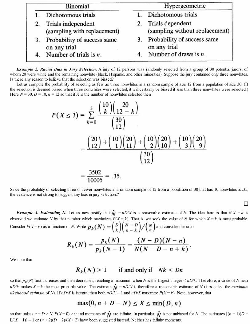
Example 2. Racial Bias in Jury Selection. A jury of 12 persons was randomly selected from a group of 30 potential jurors, ofwhom 20 were white and the remaining nonwhite (black, Hispanic, and other minorities). Suppose the jury contained only three nonwhites.Is there any reason to believe that the selection was biased?

Let us compute the probability of selecting as few as three nonwhites in a random sample of size 12 from a population of size 30. (Ifthe selection is deemed biased when three nonwhites were selected, it will certainly be biased if less than three nonwhites were selected.)Here N = 30, D = 10, n = 12 so that if X is the number of nonwhites selected then

Since the probability of selecting three or fewer nonwhites in a random sample of 12 from a population of 30 that has 10 nonwhites is .35,the evidence is not strong to suggest any bias in jury selection.?

Example 3. Estimating N. Let us now justify that = nD/X is a reasonable estimate of N. The idea here is that if X = k isobserved we estimate N by that number which maximizes P(X = k). That is, we seek the value of N for which X = k is most probable.

Consider P(X = k) as a function of N. Write and consider the ratio

We note that

so that pk(N) first increases and then decreases, reaching a maximum when N is the largest integer < nD/k . Therefore, a value of N nearnD/k makes X = k the most probable value. The estimate = nD/X is therefore a reasonable estimate of N (it is called the maximumlikelihood estimate of N). If nD/X is integral then both nD/X – 1 and nD/X maximize P(X = k). Note, however, that

so that unless n + D > N, P(X = 0) > 0 and moments of are infinite. In particular, is not unbiased for N. The estimates [(n + 1)(D +l)/(X + 1)] – 1 or (n + 2)(D + 2)/(X + 2) have been suggested instead. Neither has infinite moments.

In particular, let k = 2, n = 3, and D = 3. Then = 3(3)/2 = 4.5 so that we choose n = 4 as our estimate of N. The probabilityfunction of X gives

so that k = 2 does have the larger probability.In many problems N is known and the object is to estimate D. For example, the hypergeometric distribution has been used as a model

for the number of children attacked by an infectious disease when a fixed number N are exposed to the disease. In this case the interest isin estimating D, given N, n and X = k . We apply the same argument as above, except that we consider P(X = k) as a function of D.Consider the ratio

Note that

Hence X = k is most probable for D = where is the largest integer < k(N + 1)/n. If k(N + l)/n is integral then either (k(N + l)/n) – 1or k(N + l)/n is our estimate of D.

Example 4. Sampling Inspection. A manufacturer buys silicon chips in lots of 25. In order to check the quality of each lot he put arandomly chosen sample of size 4 from each lot to test. Let X be the number of defective chips in the sample. The following criterion isused: If X ≤ 1, accept the lot; reject otherwise. Find the probability that a lot containing five defective chips will be accepted.

Here N = 25, n = 4. If D is the actual number of defectives in a lot, then X has hypergeometric distribution:

Hence the probability of accepting a lot that has D defectives is given by

In particular, when D = 5,

Hence the manufacturer has an 83 percent chance of accepting a lot containing five defective chips. In fact, even if he adopts the rule:

he has about a 38.3 percent chance of accepting a lot with five defective chips.

Yet another question of interest is the following. Suppose a lot containing D defectives is acceptable.The manufacturer takes a random sample of size n and puts the items to test. When should a lot be rejectedif the manufacturer is willing to allow an error of at most 100α percent of rejecting an acceptable (good)lot?

In this case, we need to find the smallest c such that

The lot is rejected if we observe c, c + 1,…, min(n, D) defectives in the sample and accepted otherwise.For example, let us take N = 20, D = 2, n = 3, and α = 0.5. Then we need to choose the smallest c suchthat

These probabilities are given below:

It follows that c = 2.Finally, we show that we can approximate hypergeometric probabilities by binomial probabilities.

Example 5. Approximating Hypergeometric by Binomial We note that the computation of P(X = k) from (1) becomescumbersome when N is large. If N is very large (infinite) it does not matter whether we sample with or without replacement. The trialswill then be almost independent and we should expect to approximate P(X = k) by a binomial probability. Indeed, if N is large then p D/N and we should be able to approximate (1) by

Clearly, we cannot let N → ∞ and D fixed since then D/N → 0. So we need N → ∞, D → ∞ such that D/N → p, 0 < p < 1. To see whatother conditions we need in order that

let us rewrite (1) as

Let N → ∞, D → ∞ such that D/N → 0 < p < 1. The middle term then → pk . The third term will converge to (1 – p)n–k provided n issmall compared with N (note that k < n). Then

The approximation is considered adequate when N > 50 and n/N ≤ .10. Since binomial probability can be approximated by Poisson ornormal distribution, as we shall show, hypergeometric probabilities can also be approximated by Poisson and normal probabilities.

Let us show how good the binomial approximation is. We first apply binomial approximation to the data of Examples 2 and 4 eventhough the conditions for validity of the approximation are not satisfied. In Example 2, p D/N = 10/30 and n = 12 so that

In Example 4, p D/N = 5/25 = .20 and n = 4, so that

Neither approximation is that bad even though N < 50 and n/N > .1 in each case.It should be noted that in (1) D and n can be interchanged without changing the distribution of X. This gives us another binomial

approximation for P(X = k), but with p = n/N.

Approximating Hypergeometric Probability, P(X = k)

It turns out that there are two more approximations possible due to another symmetry (see Problem 9). But we are not going to pursue thesubject any further.

In Table 1 we give the exact probability under hypergeometric and the corresponding binomial approximation.

TABLE 1. Binomial Approximation to Hypergeometrica

a Hypergeometric probabilities are taken from G. J. Lieberman and D. B. Owen, Tables of Hypergeometric Probability Distribution ,Stanford University Press, 1961, with permission.

We now compute the mean and the variance of a hypergeometric distribution. We will need thefollowing identities.

To prove (4) we note that

in view of (2). To prove (5) we apply the same procedure. Indeed,

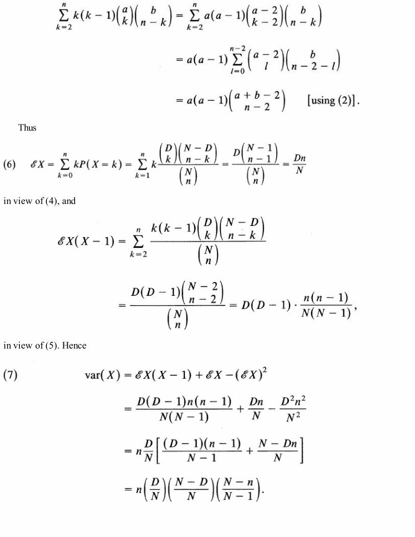
Thus

in view of (4), and

in view of (5). Hence

Mean and Variance of Hypergeometric Distribution

If we let D → ∞, N → ∞ such that D/N → p, 0 < p < 1, then

provided n/N → 0. These are the mean and variance of the limiting binomial distribution. whenever n/Nis not small,

The factor (N → n)/(N → 1) is called (see Example 5.3.1) the finite population correction factor for thevariance in sampling without replacement. If N is large compared with “, this factor is approximately 1since, in that case, sampling with or without replacement are about the same.

Example 6. Election Reversal This novel application of hypergeometric distribution is due to Finkelstein and Robbins.† Consider anelection with two candidates, A and B, where A receives a votes and B receives b votes, a > b. Suppose n of the total N = a + b votescast were irregular (illegal). Candidate B challenges the result of the election, claiming that if these n votes were to be removed at randomthe outcome may result in a reversal of the election result. Let us compute the probability of a reversal.

Suppose these n votes are removed at random from the N votes cast. Let X be the number of these votes for Candidate A and hencen – X for Candidate B. Then a reversal occurs if and only if

that is, if and only if

Since X is a random variable that is not observed [all we know is the triple (a, b, n)] there is no way to check if

We first note that X has a hypergeometric distribution with N = a + b, D = a, and n = n, so that:

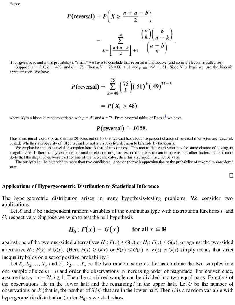
Hence

If for given a, b, and n this probability is “small,” we have to conclude that reversal is improbable (and no new election is called for).Suppose a = 510, b = 490, and n = 75. Then n/N = 75/1000 < .1 and p a/N = .51. Since N is large we use the binomial

approximation. We have

where X1 is a binomial random variable with p = .51 and n = 75. From binomial tables of Romig† we have

Thus a margin of victory of as small as 20 votes out of 1000 votes cast has about 1.6 percent chance of reversal if 75 votes are randomlyvoided. Whether a probability of .0158 is small or not is a subjective decision to be made by the courts.

We emphasize that the crucial assumption here is that of randomness. This means that each voter has the same chance of casting anirregular vote. If there is any evidence of fraud or election irregularities, or if there is reason to believe that other factors made it morelikely that the illegal votes were cast for one of the two candidates, then this assumption may not be valid.

The analysis can be extended to more than two candidates. Another (normal) approximation to the probability of reversal is consideredlater.

Applications of Hypergeometric Distribution to Statistical Inference

The hypergeometric distribution arises in many hypothesis-testing problems. We consider twoapplications.

Let X and Y be independent random variables of the continuous type with distribution functions F andG, respectively. Suppose we wish to test the null hypothesis

against one of the two one-sided alternatives H1: F(x) ≥ G(x) or H1: F(x) ≤ G(x), or against the two-sidedalternative H1: F(x) ≠ G(x). (Here F(x) ≥ G(x) or F(x) ≤ G(x) or F(x) ≠ G(x) simply means that strictinequality holds on a set of positive probability.)

Let Xl, X2,…, Xm and Y1, Y2,…, Yn be the two random samples. Let us combine the two samples intoone sample of size m + n and order the observations in increasing order of magnitude. For convenience,assume that m + n = 2l, l ≥ 1. Then the combined sample can be divided into two equal parts. Exactly l ofthe observations He in the lower half and the remaining l in the upper half. Let U be the number ofobservations on X (that is, the number of Xi’s) that are in the lower half. Then U is a random variable withhypergeometric distribution (under H0 as we shall show.

Under H0, F = G so that we expect the X’s and Y’s to be evenly spread out in the combined sample. Ifwe observe a large value of U, it would be reasonable to suspect that X’s tend to be smaller than the Y’sso that P(X > x) ≤ P(Y > x) or F(x) ≥ G(x). Thus a large value of U supports the alternative F(x) ≥ G(x).Similarly, a small value of U supports the alternative F(x) ≤ G(x). A test based on U is called a mediantest since U is the number of X’s that are smaller than the sample median (which may be taken to be theaverage of the two middle values).

Let us now compute the distribution of U under H0 : F(x) = G(x) for all x ∈ . Since X and Y are ofthe continuous type, P(Xi = Yj = 0 for all i, j and we can assume that equality does not hold for any of themn pairs (Xi, Yj. The total number of samples of size l from a population of size 2l is . Let us now

count the number of those samples (of size l) in which exactly u values of X (and hence l – u values of Y)appear below the sample median. This number is . Hence

where 2l = m + n. The same argument applies in the case when m + n = 2l + 1 is an odd integer. (In thiscase there is a unique middle value, the (l + l)st value in the ordered arrangement, which is the samplemedian.)

Median Test for Testing H0:F = G

Order the combined sample of m + n observations in increasing order of magnitude. Let u0be the observed number of X’s that are smaller than the sample median.

Example 7. Comparing Two Sections of a Statistics Course . Two large sections of an elementary statistics course are taught bytwo instructors. At the end of the quarter a standard test is given to the two sections. It is desired to compare the performance of thestudents in the two sections. Since the classes were very large, a random sample of 10 students each was chosen and their scores wererecorded as follows:

Let us analyze the data to see if there is any difference in student performance.Arranging the grades in increasing order of magnitude, we have:

The sample median here is (84 + 85)/2 = 84.5, and there are five students from Section A who have a score less than 84.5. Hence U= 5. Under H0 that the distribution of scores in two sections is the same:

and

so that in random sampling there is a 67 percent chance of observing a value of U as small as (or as large as) 5. There is no evidencetherefore to reject H0 : F = G.

Another application of hypergeometric distribution is in testing the equality of two proportions. Let Xbe binomial with parameters n and pl and let Y be binomial with parameters n and p2. Suppose X and Yare independent and we wish to test H0: px = p2 against, say, H1 : p1 < p2. Let k = kl + k2 be the number ofsuccesses in m + n trials. Under H0, p1 = p2 = p so that:

Moreover,

and

Hence

which is hypergeometric. We note that under H0 the conditional distribution of X given X + Y = k isindependent of the common value p1 = p2 (which is unknown).

It is instructive to derive (9) directly as follows. The k successes in m + n trials can be divided intotwo mutually exclusive categories, those happening in the first m trials and those happening in the last ntrials. Hence the conditional distribution of the number of successes in the first m trials (the last n trials)given X + Y = k has a hypergeometric distribution given by (9).

Returning now to the problem of testing H0 : pl = p2 against H1: p1 < p2, we note that given k, a largevalue of X tends to support H0 and a small value of X tends to support H1. It is therefore reasonable toreject H1 when k1 is large (that is, the observed value of X is large). This is the Fisher–Irwin test forcomparing two unknown probabilities.

Example 8. Comparing Attitudes Towards ERA . Independent random samples of 10 male and 10 female students at a juniorcollege were asked whether or not they are in favor of the Equal Rights Amendment to the State Constitution. If six men and eightwomen favor the amendment, is there evidence to support the claim that the proportion of female students favoring ERA is more than theproportion of male students favoring ERA?

If P1, P2 respectively are the proportions of males and females favoring ERA at the college, then we wish to test H0 : p1 = p2 againstHl : p2 > P1. We have k = 6 + 8 = 14, k1 = 6, m = 10 = n. We reject H0 if X is too small. Under H0,

Since the observed event is quite probable under H0, we cannot reject H0. That is, the evidence does not support the claim that p2 > p1

Problems for Section 6.4

1. Ten vegetable cans, all of the same size, have lost their labels. It is known that four contain tomatoesand six contain peas.(i) What is the probability that in a random sample of four cans all contain tomatoes?(ii) What is the probability that two or more contain peas?

2. An urn contains nine marbles of which three are red, three green, and three yellow. A sample of size4 is taken (without replacement).(i) Find the probability that the sample will contain marbles of:

(a) Only two colors. (b) All three colors.(ii) What is the expected number of colors in the sample?(iii) What is the probability distribution of red marbles in the sample?(iv) How large a sample must you take so that the probability is at least .90 that it will contain all

three red marbles?3. A lot of 10 light bulbs contains two defective bulbs. A random sample of five bulbs is inspected

from the lot.(i) What is the probability that the sample contains at least one defective?(ii) What is the minimum number of bulbs that should be examined so that the probability of finding

at least one defective is at least 1/2? At least .80?4. A shipment of 50 items is received. The shipment is accepted if a random sample of five items

inspected shows fewer than two items defective.(i) If the shipment contains five defectives, what is the probability that it will be accepted?(ii) What is the probability of accepting a shipment containing 15 defectives? 30 defectives?

5. From a group of 10 (five men and five women) a committee of four was selected randomly. Allcommittee members selected were men. Is there evidence to question the randomness of theselection?

6. Suppose 40 cards marked 1, 2, …, 40 are randomly arranged in a row. Find the distribution of thenumber of even integers in the first 25 positions.

7. There are 58 Republicans and 42 Democrats in the U.S. Senate. A committee of three Senators is tobe chosen at random. Find the probability that:(i) All members of the committee are from the same party.(ii) The committee consists of at least one democrat.(iii) The committee consists of at least one member of each party.

8. From a deck of bridge cards, five cards are drawn at random. Find the probability that:(i) All five cards are of red suits.(ii) All five cards are face cards.(iii) All four aces are drawn.

9. Let us write p(k, n; N, D) for

Show that D and n can be interchanged without changing P(X = k). That is, show that(i) p(k, n; N, D) = p(k, D; N, n),(ii) p(n – k, N – D; N, n) = p(D – k, N – n; N, D).

10. Consider the estimate = X(N + l)/n of D. Is unbiased for D? (That is, check if = D.) Findvar( ). (See also Problem 13.)

11. Is it possible for a hypergeometric random variable X that X = var(X)?12. Let X and Y be random variables such that X is binomial with parameters m and p and

(i) Find the unconditional distribution of Y.(ii) Find the conditional distribution of X given X = y.

13. Show that:(i) = NX/n is an unbiased estimate of D.(ii) X/n is an unbiased estimate of D/N so that estimation of D/N, the fraction of defectives, does not

require knowledge of N.In particular, suppose that a random sample of 100 voters in a county showed 29 Republicans. Whatis an unbiased estimate of the proportion of Republican voters in the county? If it is known that thecounty has 6000 voters, what is an unbiased estimate of the number of Republican voters?

14. Find an upper bound for P(X/n – D/N| ≤ ε), where X is hypergeometric and ε > 0.15*. Letp(k, N; n, D) be the probability of drawing k defectives in a random sample of size n from a

population of N elements containing D defectives. Since sampling without replacement is equivalentto sampling one after another, consider the last draw. It produces either a defective or anondefective item. Show that

Use this relation to show that

and also to derive the mean and variance of p(k, N; n, D).16. In order to study the efficacy of a drug to control hyperactivity in children under age 8, ten children

chosen randomly were given the drug, and ten different children, also chosen randomly (andindependently of the first group), were given a placebo. All 20 children were then given a test whichwas scored on an ordinal scale with the following results (higher score indicates higher level ofhyperactivity).

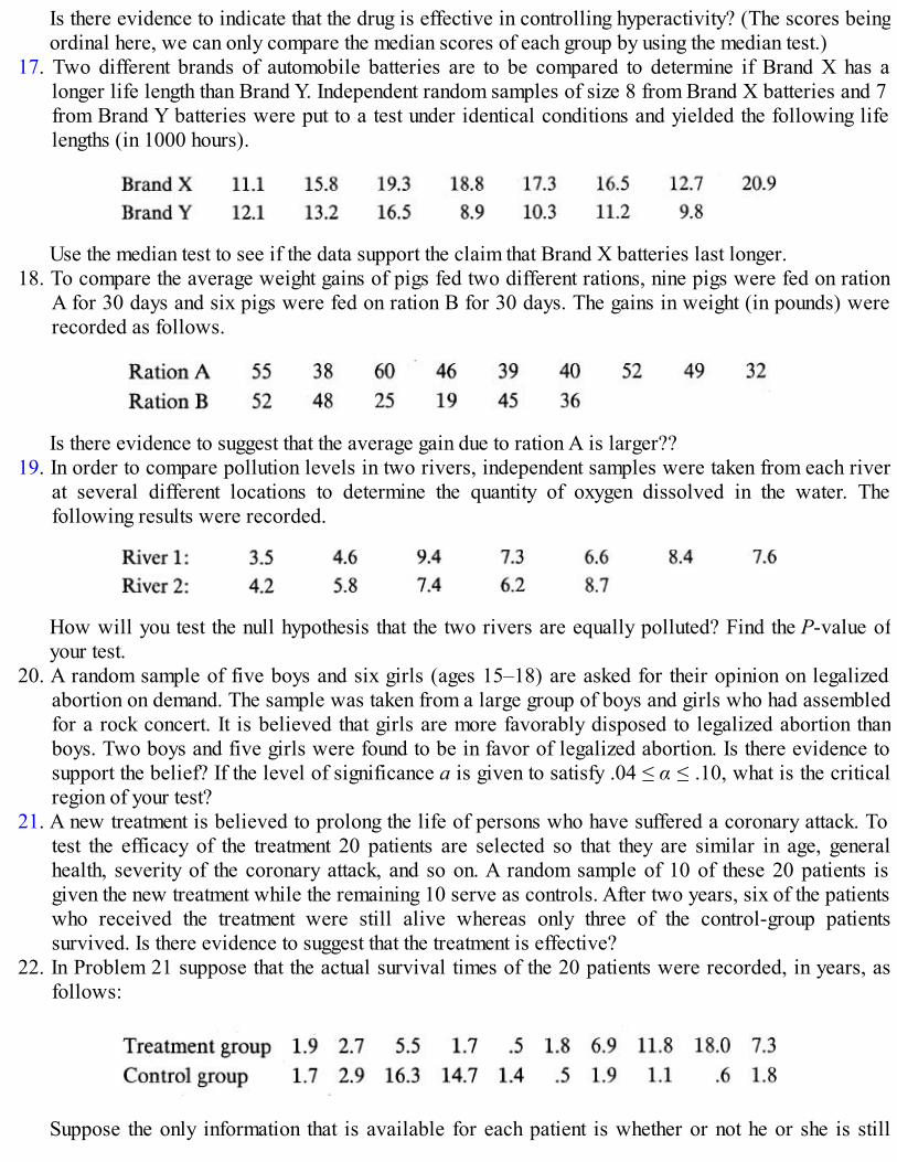
Is there evidence to indicate that the drug is effective in controlling hyperactivity? (The scores beingordinal here, we can only compare the median scores of each group by using the median test.)

17. Two different brands of automobile batteries are to be compared to determine if Brand X has alonger life length than Brand Y. Independent random samples of size 8 from Brand X batteries and 7from Brand Y batteries were put to a test under identical conditions and yielded the following lifelengths (in 1000 hours).

Use the median test to see if the data support the claim that Brand X batteries last longer.18. To compare the average weight gains of pigs fed two different rations, nine pigs were fed on ration

A for 30 days and six pigs were fed on ration B for 30 days. The gains in weight (in pounds) wererecorded as follows.

Is there evidence to suggest that the average gain due to ration A is larger??19. In order to compare pollution levels in two rivers, independent samples were taken from each river

at several different locations to determine the quantity of oxygen dissolved in the water. Thefollowing results were recorded.

How will you test the null hypothesis that the two rivers are equally polluted? Find the P-value ofyour test.

20. A random sample of five boys and six girls (ages 15–18) are asked for their opinion on legalizedabortion on demand. The sample was taken from a large group of boys and girls who had assembledfor a rock concert. It is believed that girls are more favorably disposed to legalized abortion thanboys. Two boys and five girls were found to be in favor of legalized abortion. Is there evidence tosupport the belief? If the level of significance a is given to satisfy .04 ≤ α ≤ .10, what is the criticalregion of your test?

21. A new treatment is believed to prolong the life of persons who have suffered a coronary attack. Totest the efficacy of the treatment 20 patients are selected so that they are similar in age, generalhealth, severity of the coronary attack, and so on. A random sample of 10 of these 20 patients isgiven the new treatment while the remaining 10 serve as controls. After two years, six of the patientswho received the treatment were still alive whereas only three of the control-group patientssurvived. Is there evidence to suggest that the treatment is effective?

22. In Problem 21 suppose that the actual survival times of the 20 patients were recorded, in years, asfollows:

Suppose the only information that is available for each patient is whether or not he or she is still

alive after five years. Is there any evidence to suggest that the treatment prolongs the life of patients?23. Of 25 income tax returns audited in a small town, 10 were from low and middle income families and

15 from high income families. Two of the low income families and four of the high income familieswere found to have underpaid their taxes. Are the two proportions of families who underpaid taxesthe same?

24. A candidate for a congressional seat checks her progress by taking a random sample of 20 voterseach week. Last week, six reported to be in her favor. This week nine reported to be in her favor. Isthere evidence to suggest that her campaign is working?

25. Two large sections of a statistics course are taught during the spring semester, Section 1 meeting inthe morning and Section 2 in the late afternoon. Students were randomly assigned to these sectionsand the same professor taught both courses using the same text. To compare the performance of thestudents, in order to determine if there were any differences due to the time of the day the classesmet, random samples of nine students each were selected. Section 1 had four A’s and Section 2 hadtwo A’s. Is the proportion of A students in Section 1 significantly larger than that in Section 2?

6.5 GEOMETRIC AND NEGATIVE BINOMIAL DISTRIBUTIONS: DISCRETEWAITING-TIME DISTRIBUTION

Suppose that a couple decides to have children until they have a girl. What is the average number ofissues needed before they have the first girl? What is the probability that they have three boys before theyhave a girl? Assuming that boys and girls are equally likely, that is, the probability that the sex of anewborn is male is 1/2, it is intuitively clear that the average number of issues needed for the first girl isl/(l/2) = 2. How do we justify this? More important, how do we compute the required probability,namely, that the fourth child is the first girl? This probability is not 1/2. It does not equal the conditionalprobability that the fourth is a girl, given that the first three children were boys. By independence, thatprobability is always 1/2 no matter what the sex distribution of the first three of their children.

We note that the experiment looks much like a binomial:

(i) There is dichotomy, either girl (success) or boy (failure).(ii) Trials are independent.(iii) The probability of success on each trial is 1 /2.

The number of trials, however, is not fixed in advance. Indeed the number of trials is a random variablewhich equals the number of times the experiment is repeated until a success occurs. We recall that in abinomial experiment, the number of trials is fixed in advance and the random variable of interest is thenumber of successes in n trials.

Let X be the number of trials needed for the first success. Then X is said to have a geometricdistribution.

Binomial or Geometric

Assumptions: (i) Dichotomous trials. (ii) Probability of success p is same on each trial. (iii) Trials are independent.

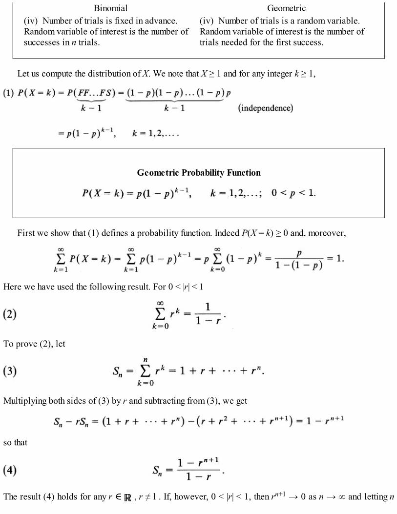
Binomial Geometric(iv) Number of trials is fixed in advance.Random variable of interest is the number ofsuccesses in n trials.

(iv) Number of trials is a random variable.Random variable of interest is the number oftrials needed for the first success.

Let us compute the distribution of X. We note that X ≥ 1 and for any integer k ≥ 1,

Geometric Probability Function

First we show that (1) defines a probability function. Indeed P(X = k) ≥ 0 and, moreover,

Here we have used the following result. For 0 < |r| < 1

To prove (2), let

Multiplying both sides of (3) by r and subtracting from (3), we get

so that

The result (4) holds for any r ∈ , r ≠ l . If, however, 0 < |r| < 1, then rn+1 → 0 as n → ∞ and letting n

→ ∞ in (4) we have

We also need the following identities: For 0 < r < 1

To prove (5) we differentiate both sides of (2) with respect to r. We have

To prove (6), we differentiate (5) with respect to r to obtain

Using (5) and (6) we have

and

Hence

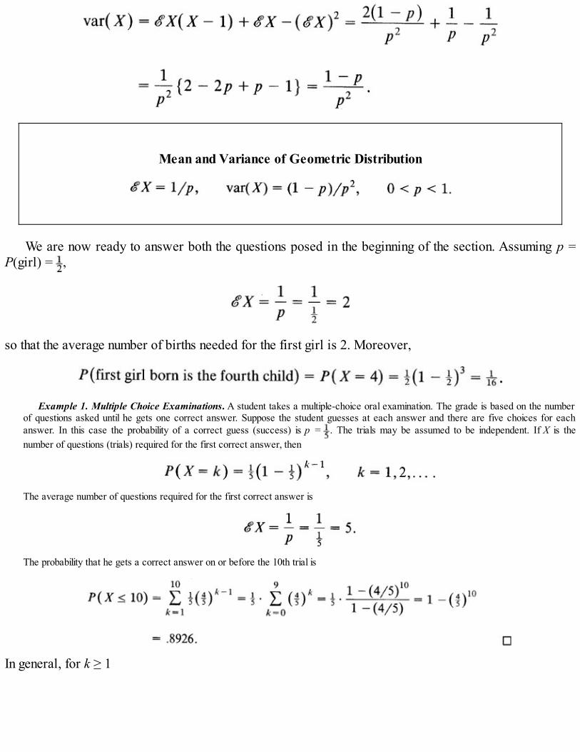
Mean and Variance of Geometric Distribution

We are now ready to answer both the questions posed in the beginning of the section. Assuming p =P(girl) = ,

so that the average number of births needed for the first girl is 2. Moreover,

Example 1. Multiple Choice Examinations. A student takes a multiple-choice oral examination. The grade is based on the numberof questions asked until he gets one correct answer. Suppose the student guesses at each answer and there are five choices for eachanswer. In this case the probability of a correct guess (success) is p = . The trials may be assumed to be independent. If X is thenumber of questions (trials) required for the first correct answer, then

The average number of questions required for the first correct answer is

The probability that he gets a correct answer on or before the 10th trial is

In general, for k ≥ 1

so that†

and

We note that for integers k, l ≥ 1, we have from (7)

where we have used the fact that

so that {X > k + l} ⊆ {X > l}. Hence {X > k + l, X > l} = {X > k + l} ∩ {X > l} = {X > k + l}. Equation(9) has the following interpretation. Given that the first success happens after the lth trial (that is, nosuccess was observed in the first l trials), the conditional probability that the first success will beobserved after an additional k trials depends only on k. This is the so-called lack of memory property ofa geometric law. The process forgets the initial string of l failures. This is a characterizing property of ageometric probability function. That is, any positive integer-valued random variable satisfying (9) musthave a geometric distribution (Problem 28).

Example 2. Number of Trials Required to Achieve a Success . In many applications, one is interested not in the average number oftrials but the number of trials required to observe the first success with a given probability. That is, for given α, 0 < α < 1, usually small, wewish to find n such that

In view of (8) we have

so that

Taking logarithms and solving for n we see that

Thus, if p = and α = .05 so that we want to be 95 percent sure of achieving a success in n trials with a fair coin, then we must choose

Hence with a fair coin we are 95 percent certain to achieve a success in five (or more) trials.

Example 3. Estimating p. Yet another question of interest is to estimate p. Suppose we need n trials to achieve a success. Then

The most probable value of n is obtained by maximizing P(X = n) with respect to p. Thus

gives = l/n as our estimate of p. Note that

so that p = l/n is a maximum. In particular, if we need 90 tosses to achieve a success, then our estimate of p is Note, however, that the estimate = 1/X is not unbiased. In fact,

It is well known that the Taylor series expansion of ln(l + t) for |t| < 1 is given by

so that on replacing t by –t we have

Hence with t = 1 – p, 0 < p < 1, we have

and it follows that = 1/X is not an unbiased estimate of p. It can be shown (Problem 29) that there does not exist an unbiased estimateof p.

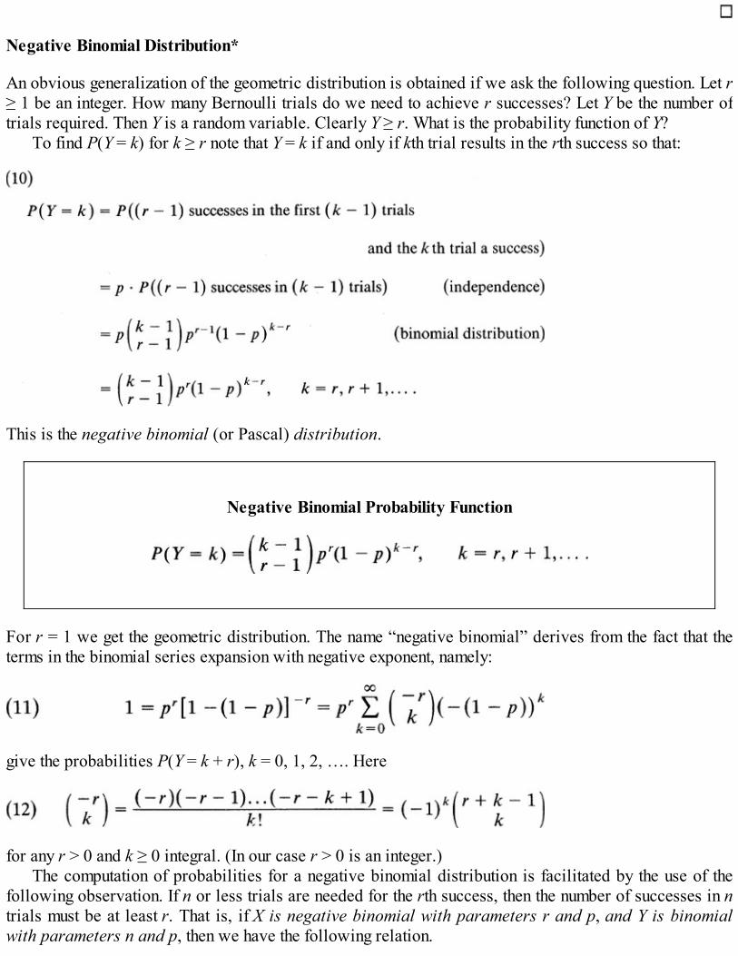
Negative Binomial Distribution*

An obvious generalization of the geometric distribution is obtained if we ask the following question. Let r≥ 1 be an integer. How many Bernoulli trials do we need to achieve r successes? Let Y be the number oftrials required. Then Y is a random variable. Clearly Y ≥ r. What is the probability function of Y?

To find P(Y = k) for k ≥ r note that Y = k if and only if kth trial results in the rth success so that:

This is the negative binomial (or Pascal) distribution.

Negative Binomial Probability Function

For r = 1 we get the geometric distribution. The name “negative binomial” derives from the fact that theterms in the binomial series expansion with negative exponent, namely:

give the probabilities P(Y = k + r), k = 0, 1, 2, …. Here

for any r > 0 and k ≥ 0 integral. (In our case r > 0 is an integer.)The computation of probabilities for a negative binomial distribution is facilitated by the use of the

following observation. If n or less trials are needed for the rth success, then the number of successes in ntrials must be at least r. That is, if X is negative binomial with parameters r and p, and Y is binomialwith parameters n and p, then we have the following relation.

Relation Between Negative Binomial and Binomial

Consequently, we can use Table A3 for binomial probabilities to compute probabilities under negativebinomial (or geometric) distribution. Figure 1 shows some histograms for negative binomial distribution.

Figure 1. Historram for negative binomial

The mean and the variance are easily computed. We have

in view of (12) and (11). Similarly,

Hence

Mean and Variance of Negative Binomial Distribution

Example 4. Selecting Mice for a Laboratory Experiment. In many laboratory experiments involving animals, the experimenterneeds a certain number of animals. Suppose an experimenter needs five mice that have a certain disease. A large collection of mice isavailable to him, and the incidence of disease in this population is 30 percent. If the experimenter examines mice one at a time until he getsthe five mice needed, then the number of mice X that must be examined has a negative binomial distribution with p = .3 and r = 5. Theexpected number of examinations required is r/p = 5/.3 = 16.67. The probability that the number of examinations required is more than 25is given by

where Y is binomial with parameters n = 25 and p = .3. From Table A3

so that there is only about a 9 percent chance that more than 25 examinations will be required to get five mice that have the disease.

Example 5. The World Series of Baseball. In the World Series, two baseball teams A and B play a series of at most seven games.The first team to win four games wins the series. Assume that the outcomes of the games are independent. Let p be the (constant)probability for team A to win each game, 0 < p < 1. Let X be the number of games needed for A to win. Then 4 ≤ X ≤ 7. Writing

we note that Ak ∩ Al = ϕ, k ≠ l, so that

where

Hence,

In particular, let p = 1/2. Then P(A wins) = 1/2. The probability that A will win in exactly six games is . The probability

that A will win in six games or less is 11/32.Given that A has won the first two games, the conditional probability of A winning the series equals

Given that A has won two and lost three of the first five games, the probability that A will win is .

The negative binomial distribution is frequently referred to as a waiting time distribution since it maybe interpreted as the probability distribution of the waiting time for the rth success. Let Sk = X1 + ··· +Xk be the number of trials necessary for the kth success, k = l, 2, …, r. Then we can think of Sr as the sumo f r independent and identically distributed random variables X1, … , Xr each having a geometricdistribution with parameter p (see Figure 2). Each Xi is a waiting time for one success. Thus X1 is thewaiting time for first success, X2 is the waiting time for an additional success, and so on. Conversely, thesum of r independent identically distributed geometric random variables can be imagined as the numberof trials necessary for the rth success and, hence, must have a negative binomial distribution. A formalproof is given in Chapter 8. A continuous analog of negative binomial (and geometric) distribution isconsidered in Section 7.4.

Figure 2

Finally, we consider briefly an analogue of the negative binomial distribution in sampling withoutreplacement. Considering the urn model with w white and b black marbles, if we sample withreplacement and ask for the distribution of the number of draws X needed for the rth black marble, then Xhas the negative binomial distribution

If we sample without replacement one after the other, then in order that the kth draw (k ≥ r) be the rthblack marble drawn, the kth draw must produce a black marble whereas in the previous k – 1 draws theremust have been (r – 1) black marbles. Hence:

k = r, r + 1,…, b + w.Rewriting (14) we see that

A simple argument now shows that P(X = k) as given by (15) or (14) approaches

as b + w → ∞ provided that r/(b + w) → 0 and k/(b + w) → 0 (Problem 24). This is precisely theprobability given in (13) as we expect, since when b + w → ∞ sampling with or without replacement isthe same. [Although (15) looks much like the hypergeometric probability (6.4.1), it is not the same.]

In the case of dichotomous trials we have considered four probability distributions. Let us summarizethe results.

Dichotomous Trials

(i) Independent, identical trials with constant probability p of success

(ii) Dependent trials

Problems for Section 6.5

Problems 16–27 refer to the Subsection on negative binomial distribution.1. A fair die is rolled until an ace shows up.

(i) Find the probability of the first ace showing up on the sixth trial.(ii) Find the probability that an ace shows up in at most six trials.(iii) Find the number of trials required so that the probability of getting an ace is at least 1/2.

2. About 5 percent of potatoes grown by a farmer have rotten centers. In order to test whether a potatois rotten, one has to cut it open. Find the probability that:(i) The ninth potato cut is the first rotten potato.(ii) Twenty-five or more potatoes have to be destroyed to find the first rotten potato.

3. A test yields a positive reaction with probability .7. What is the probability that the first positivereaction occurs after nine negative reactions?

4. About 90 percent of apples grown by a farmer are good. It is not possible to detect a rotten applewithout cutting the apple. If 15 good apples are needed to bake a pie, what is the probability that in arandom selection 20 or more apples must be cut open?

5. Three people are having coffee in a diner. They each toss a coin to determine the odd person, who isthen asked to pay. Tosses are continued until a decision is reached. Let p be the probability ofsuccess on each coin. Find the probability that fewer than n tossings are necessary to reach adecision.

In particular, if p = 1/2 find the minimum number of tossings required to reach a decision in 90percent of the cases.

6. In a series of independent Bernoulli trials, it is known that the average number of trials needed for asuccess is 10. Find the distribution of the number of trials needed to achieve a success. Also find thedistribution of the number of successes in 10 trials.

7. (i) In successive tossings with a fair die, find the probability of an ace before an even-numbered facevalue.

(ii) Answer part (i) if the die is loaded such that P(l) = p, P(2) = P(4) = P(6) = pl with 0 < p + 3p1 <

1, p, p1 > 0.8. Consider a series of independent Bernoulli trials. If the mean number of successes is five and the

mean number of trials needed to achieve a success is also five, find the distribution of:(i) The number of successes.(ii) The number of trials needed to achieve a success.

9. A motorist encounters n consecutive lights. Each of the lights is equally likely to be green or red.Find the probability distribution of the number of green lights passed by the motorist before beingstopped by a red light.

10. The number of times X that a light switch operates before being discarded has probability function

(i) Find the probability that the number of times the switch operates is an even number.(ii) Find the probability that the number of times the switch operates is an integral multiple of 3.

11. A lot of television tubes is tested by randomly testing tubes one after another until a defective tube isfound. The number of tubes tested determines whether or not the lot is accepted. Let k be the criticalnumber, that is, the lot is accepted if k or more tubes are tested for the first defective.(i) Find the probability that a lot containing a proportion p of defectives will be accepted.

(ii) If k = 5 and p = .10 find the probability of accepting the lot.(iii) What should be the value of k if we want to be 90 percent confident of rejecting a lot that has 25

percent defectives?12. Families with two children are required for a psychological study. The following sampling scheme

is used. Randomly selected families (with two children) are interviewed sequentially until the firstfamily with two boys appears for an interview. No more families are interviewed after that.(i) What is the average number of families selected using this procedure?(ii) What is the probability that more than 10 families will be selected for this study?(iii) What is the probability that four families will be selected?

13. A pair of identically loaded coins are thrown together independently. Let p be the probability of ahead on each coin. What is the distribution of number of throws required for both coins to show headsimultaneously? What is the distribution of number of throws required for at least one of the coins toshow a head?

14. A fair die is rolled repeatedly. What is the probability that a face value of 2 will show up before aface value of 5?

15. A pair of fair dice is rolled repeatedly. Find the probability that a sum of face values of 7 appearsbefore a sum of face values of 4.

16. A baseball player has a season batting average of .300 going into the World Series. He needs 10more hits to reach a season total of 150 hits. What is the probability that 12 or less times at bat arerequired to reach his goal? Does he have a reasonable chance of reaching his goal this season?

17. A student takes a five-answer multiple-choice oral test. His grade is determined by the number ofquestions required in order for him to get five correct answers. A grade of A is given if he requiresonly five questions; a grade of B is given if he requires 6 or 7 questions; a grade of C is given if herequires 8 or 9 questions; he fails otherwise. Suppose the student guesses at each answer. What isthe probability of his getting an A? B? C?

18. In repeated tossings of a pair of fair dice, find the probability that the sum of face values is 7 twicebefore a sum of 4. What is the probability of two successive sums of 7 before a sum of 4? [Hint:P(sum of 7 before a sum of 4) = from Problem 15.]

19*. The game of craps is played with two fair dice as follows. A person throws the pair of dice. He

wins on the first throw if he gets a sum of 7 or 11, loses if he throws 2, 3, or 12, and continues tothrow otherwise until he throws a sum of 7 or the first number thrown. He wins if he throws the firstnumber thrown and loses if 7 appears. (See also Problem 2.7.18.)(i) Find the probability of winning for the player.(ii) Find the expected number of throws required before the game ends.

20. In a sequence of independent Bernoulli trials with probability p of success, find the probability thatn1 successes will occur before n2 failures.

21*. Let q(n, r; p) be the probability of observing the rth success on the nth trial with constantprobability p of success. By considering the result of the nth trial, show that

Hence show (by induction) that

Find X and var(x) for the distribution q(n, r; p) by using the recursive relation [q(n, r; p) = 0 for n< r].

22. There are N marbles numbered 1 through N in an urn. Marbles are drawn one after another withreplacement. Let X be the number of drawings until the first marble is drawn again. Find thedistribution and expected value of X.

23. Consider a biased coin with probability p of heads, 0 < p < 1. The coin is tossed once. If a headshows up it is tossed until another head shows up. Let X be the number of trials needed to stop. Findthe distribution of X, its mean and its variance.

24. Show that the probability function (14) or (15) → negative binomial probability function as b + w →∞. That is, show that

where k and r are fixed constants.25. (i) Show that for n ≥ r

where Xl, X2, …, Xr are independent identically distributed geometric random variables withcommon parameter p. In particular, P{X1 = k | X1 + X2 = n} is uniform on {1, 2,…, n – 1}.(ii) Show that for any l ≥ 2, the conditional distribution of X1 + ··· + Xl – l given X1 + ··· + Xl = n is

given by

26*. Let X have a negative binomial distribution with parameters r and p.(i) Given r andp, for what value of k is P(X = k) maximum? That is, what is the most probable value

of X?(ii) Show that = r/X is the estimate of p that maximizes P(X = k).(iii) Show that = r/X is not unbiased for p but that l = (r – l)/(X – 1) is unbiased for p (provided r

≥ 2). (See Example 3.)(iv) Given p., find the estimate of r that maximizes P(X = k).(v) Given p, find an unbiased estimate of r.[Hint: For (i) consider P(X = k)/P(X = k – 1). For (ii) consider P(X = k) as a function of p. For (iv)consider P(X = k) as a function of r and use an argument similar to that of (i).]

27*. Since (15) defines a probability distribution, it follows that

and on rewriting with l = k – r,

Use this identity to show that

and

28*. Show that the lack of memory property characterizes a geometric distribution. That is, let X be a(positive) integer valued random variable with 0 < P(X = 1) < 1. If for all integers k, l > 1

then Xmust have a geometric distribution. (Hint: Iterate P{X > k + 1} = P{X > l}P{X > k}.)29*. Show that if X has a geometric distribution with parameter p, then there does not exist an unbiased

estimate of X = 1/p. [Hint: If h(x) is unbiased for 1/p, then h{X) = 1/p for all p, 0 < p < 1.Compare coefficients of various powers of p on both sides.]

6.6 POISSON DISTRIBUTION

Another probability distribution which is closely connected to the binomial distribution often arises inpractice. This is the distribution of the number of occurrences of a rare event, that is an event with smallprobability p, in n independent trials. It is called the Poisson distribution. Typical examples are thenumber of customers that enter a store during a 15-minute interval, the number of machine failures per dayin a plant, the number of printing errors per page of a book, the number of winning tickets among thosepurchased in a state lottery, the number of motorists arriving at a gas station per hour, the number oftelephone calls at an exchange per hour, the number of errors that a typist makes per page, the number ofradioactive particles that decay per unit time, and so on. In all these examples, the event of interest is rare(per unit of time, space, or volume).

To find the probability function of the number of rare events we need to make certain assumptions. LetX(Δ) be the number of events that occur during an interval Δ. We assume that

(i) The events are independent; this means that if Δ1, Δ2,… are disjoint intervals then the randomvariables X(Δ1), X(Δ2),… are independent.

(ii) The distribution of X(Δ) depends only on the length of Δ and not on the time of occurrence.(iii) The probability that exactly one event occurs in a small interval of length Δt equals λ Δt + o(Δt)

where† o(Δt) → 0 as length Δt → 0, and λ > 0.(iv) The probability that two or more events occur in a small interval of length Δt is o(Δt).

In view of (iii) and (iv), the probability of zero events in a small interval of length Δt is 1 – λ Δt +o(Δt).

Consider the interval [0, t] and let X(t) be the number of events in [0, t]. Let us subdivide [0, t] in ndisjoint intervals each of length t/n. Let Δl, Δ2,…, Δn be these intervals. Then:

where X(Δk) , k = 1, 2, …, n are independent and X(t) has a binomial distribution with probabilityfunction

We need the following lemma, which describes a property of exponential functions.

LEMMA 1. Let us write f(x) = o(x) if f(x)/x → 0 as x → 0. Then

Proof. Expanding f into a Taylor series about x = 0, we have:

If f’ is continuous at 0, then as x → 0

In particular, let f(x) = ln(l + x) so that f’(x) = 1/(1 + x), which is continuous at 0. Then, as x → 0

Hence for large n,

so that

as asserted.

For fixed k we now let n → ∞ in the expression for P(X(t) = k) above. We have:

since as n → ∞

and from Lemma 1,

Hence:

where λ is called the intensity or the rate of occurrence.A similar argument shows that if X is a binomial random variable with parameters p and n then

provided n → ∞, p → 0 in such a way that np → X. It is clear that (3) is a special case of (2) with t = 1.We note that in view of (3), binomial probabilities can be approximated by Poisson probabilities.

The approximation is good provided p is small (p < .1) and np = λ is moderate† (≤ 10). In Table 1 wecompare the binomial distribution with parameters n, p and the Poisson distribution with parameter λ =np for n = 50, p = .1 and for n = 100, p = .01. Table A4 in the Appendix gives cumulative Poissonprobabilities for some selected values of λ. Figure 1 shows histograms of (3) for some selected values ofλ.

Clearly, P(X = k) > 0 and, moreover,

so that P(X = k) does define a probability function. Let us compute the mean

TABLE 1. Poisson Approximation

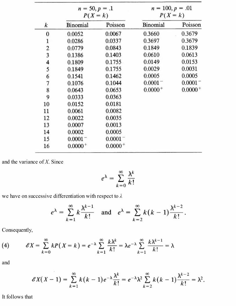
and the variance of X. Since

we have on successive differentiation with respect to λ

Consequently,

and

It follows that

Figure 1. Histogram for Poisson, λ = .5, 2, 4.

Mean and Variance of Poisson Distribution

Example 1. Probability of Hitting a Target. The probability of hitting a target with a single shot is .002. In 4000 shots, find theprobability of hitting the target more than two times.

If we identify success by a hit, then p = P(success) = .002 is small and the number of trials n = 4000 is large. Moreover, λ = np = 8 ≤

10. We can therefore apply the Poisson approximation. If X denotes the number of hits, then

Example 2. Probability of Winning in a State Lottery . Suppose M of the N lottery tickets issued by a state lottery are winningtickets. Then the probability of buying a winning ticket is p = M/N. Usually N is very large and p is small. If a person buys n tickets thenthe number of winning tickets X in the n purchased has, approximately, a Poisson distribution with parameter λ = np = nM/N and

Moreover,

If we wish to guarantee that

then

so that

That is,

so that the purchaser needs to buy at least (N/M)\n(l/α) tickets to be 100(1 – α) percent confident of having at least one winning ticket. IfM/N = 1/10,000 and α = .05, then n ≥ 29957.3, so that in a lottery where 1 out of 10,000 tickets is a winning ticket a player needs to buy29,958 tickets or more in order to be 95 percent confident of owning a winning ticket.

Example 3. Automobile Accidents at an Intersection . The number of automobile accidents at a certain intersection in a month hasapproximately a Poisson distribution with a mean of 4. What is the probability that no accidents occur in a week?

Assuming 4 weeks to a month, we note that the weekly rate of accidents is λ = 1. If X denotes the number of accidents in a week atthat intersection, then:

Also,

Thus the event that more than five accidents occur at this intersection during a week is a rare event. If more than five accidents areactually observed, we will have to suspect that the weekly rate λ ≠ 1 (that is, it is larger).

Estimation of λ and tests of hypotheses concerning λ are considered in Chapters 10 and 11.

Problems for Section 6.6

1. The number of cars crossing a bridge during a certain interval has approximately a Poissondistribution with λ = 4. Find the probability that during a randomly chosen (similar) time interval:(i) No cars will cross the bridge.(ii) Exactly three cars will cross the bridge.(iii) No more than five cars will cross the bridge.

2. The number of common colds that a randomly chosen student at a Midwestern University has in agiven academic year is a Poisson random variable with a mean of 2.6. Find the probability that arandomly chosen student has had:(i) More than 5 colds during the school year.(ii) At most 5 colds during the school year.(iii) At least one cold.

3. The number of customers X that enter a store during a one-hour interval has a Poisson distribution.Experience has shown that P(X = 0)= .111. Find the probability that during a randomly chosen one-hour interval(i) Five or more customers enter the store.(ii) Exactly one customer enters the store.(iii) No more than five customers enter the store.

4. Suppose a large number N of raisin buns of equal size are baked from a batch of dough that containsn well-mixed raisins. Let X be the number of raisins in a randomly selected bun. Find the probabilitythat a randomly selected bun will contain:(i) No raisins. (ii) At least one raisin.(iii) At least five raisins. (iv) An even number of raisins (that is, 0,2,4,…).

5. A 500-page book has 1000 misprints. Find the probability of(i) More than two misprints on a page. (ii) No misprint on a page.(iii) Less than two misprints on a page.

6. A well known television personality has committed suicide in New York. During the weekfollowing the suicide, a psychologist observes that there were 15 suicides in New York comparedwith an average of 10 per week. The psychologist attributes the extra suicides to the suggestiveeffect of the television personality’s suicide. Do the data support the psychologist’s explanation?

7. Timothy receives, on the average, five telephone calls a day. Find the probability that he willreceive:(i) Exactly five calls on a randomly selected day.(ii) Fewer than five calls.(iii) More than five calls.

8. A life insurance company estimates the probability is .00001 that a person in the 50-to-60 age groupdies during a year from a certain rare disease. If the company has 200,000 policyholders in this agegroup, find the probability that, due to death from this disease, the company must pay off during ayear:(i) More than two claims. (ii) More than five.(iii) Less than four.

9. A car salesman sells on the average A. cars per day.(i) Use Chebyshev’s inequality to show that the number of cars X sold by him on a randomly chosen

day satisfies

(ii) Suppose λ = 3. Compare the bound in (i) with the exact probability from Table A4.(iii) If λ = 3, find the probability that on a given day he will sell:

(a) At most five cars. (b) Exactly five cars.10. In a lengthy manuscript, it is found that only one-third of the pages contain no typing errors.

Assuming that the number of errors per page has a Poisson distribution, what percentage of pageshave:(i) Exactly one error? (ii) More than one error?

11. An intersection has averaged two accidents per week. Recognizing that the frequency of accidents atthis intersection is intolerable, the city administration decided to install a traffic light at thisintersection at considerable expense to the taxpayers. To check if the traffic light reduced the numberof accidents, a week was randomly selected and showed one accident.(i) Would you say that the new lights are effective?(ii) What would be your conclusion if there was one accident over a period of two weeks?(iii) One accident over a period of four weeks?

(Assume that the number of accidents at this intersection has, approximately, a Poissondistribution.)

12. Let Y have Poisson distribution with mean λ = 5. Find a simple upper bound for P(Y > 8). Compareyour result with the exact probability from Table A4.

13. Suppose customers arrive at a store at the rate of λ per hour. Then the distribution of X(t), the numberof customers arriving in [0, t], has a Poisson distribution with mean λt. Find the probability that lessthan r customers will arrive in time interval [0, x].

14. Let X have a Poisson distribution with parameter λ. Show that for n ≥ 1:(i) P(X = n) = (λ/n)P(X = n – 1). (ii)* P(X ≥ n) < λn/n!.In particular, use (ii) to show that X < eλ.[Hint: For a positive integer valued random variable X, X =

15. Find the most probable value of k for a Poisson random variable. That is, find k for which P(X = k)is maximum for a given λ. [Hint: Consider the ratio P(X = k)/P(X = k – 1).]

16. Find λ to maximize P(X = k) for a Poisson random variable X.17*. By Chebyshev’s inequality,

(i) Show that

[Hint: Consider f(λ) = (X – λ)2 – (λ/α) ≤ 0. Find the points at which the parabola f(λ) intersects theλ-axis (see Figure 2).]

(ii) In particular, let α = .05, and suppose X = 5 is the observation. Find a 95 percent confidenceinterval for λ. Also find a 75 percent confidence interval for λ.

Figure 2. for λ1(x) ≤ λ ≤ λ2(x).

18*. (Poisson as a limit of hypergeometric.) Show that

as n, N, D → ∞ such that n/N → 0 and nD/N → λ.19*. Player A observes a Poisson random variable X with parameter λ. If the outcome is x, he asks

Player B to toss a coin x times. Let p be the probability of a head (success) on any trial. Let Y be thenumber of heads that B observes.(i) Find the probability distribution of 7, its mean and variance.(ii) Suppose Player B tells you that he has observed k successes. What is the probability that he

tossed the coin x times?20*. (Poisson as a limit of negative binomial.) Let X have a negative binomial distribution with

probability function

[Substitute k = n + r in (6.5.10).] Show that as p → 1 and r → ∞ in such a way that r(l – p) → λ > 0fixed,

21*. By considering the ratio as a function of k, show that rk

reaches its maximum when k is the largest integer not exceeding n + 1 – λ(1 – P)/P

6.7 MULTIVARIATE HYPERGEOMETRIC AND MULTINOMIALDISTRIBUTIONS

We have considered some models that are appropriate for experiments where the outcomes can be putinto two mutually exclusive categories. We recall that binomial distribution arises in sampling withreplacement and that hypergeometric arises in sampling without replacement. In many applications, eachtrial results in an outcome that can be put into more than two categories of interest. This happens, forinstance, when a pollster asks the respondents if they “strongly agree,” “agree,” “disagree,” “stronglydisagree,” or are “neutral” on a certain issue.

To build a stochastic model for this problem, we consider an urn that contains k types of marbles. Letnj (> 0) be the number of marbles of type j, j = 1, 2, …, k, and let .

First consider the case when we sample without replacement and draw a random sample of size n.Let Xj be the number of type j marbles in the sample. Then 0 ≤ Xj ≤ n for j = 1, 2,…, k and so that Xl, X2, …, Xk are dependent random variables. To find the joint probability function of Xl, X2,…,Xk we first note that there are samples of size n which are all equally likely. The event {X1 = xl, X2 =x2,…, Xk = xk} happens if and only if the sample contains x1 type 1 marbles, x2 type 2 marbles,…, xk type

k marbles such that x1+ x2 + ··· + xk = n (see Figure 1). Since there are ways of choosing the type j

marbles, j = 1, 2, …, k, it follows (Rule 1, Section 2.5) that

where

Since Xk = n – X1 – ··· – Xk – 1 we can rewrite (1) as

where 0 ≤ Xj ≤ nj, j = 1, 2, …, k – 1, such that . For k = 2 we get the hypergeometricdistribution (6.4.1) with D = n1 The probability function (1) [or (2)] is known as a multivariate

hypergeometric probability function . To show that (1) [or (2)] is a probability function we need onlyequate the coefficients of xn

Figure 1

on both sides of the identity:

to get

Next we consider the case when we sample with replacement. Set pj = nj/N, j = 1, 2, …, k so that . In this case, the trials (draws) are independent each with probability pj of drawing a type j

marble. By independence, the probability of drawing x1 marbles of type 1, x2 of type 2,…, xk of type k, ina specific order (say first x1 of type 1, then x2 of type 2,…, finally xk of type k) is . Sincethere are (n/xl!x2!…xk!) ways of choosing x1 marbles of type 1,… xk of type k (Rule 4; Section 2.5) itfollows that

where 0 ≤ xj ≤ n, . and . We may rewrite (5) as

where 0 ≤ xj ≤ n, j = 1, 2, … k – 1, and . In view of the multinomial expansion

(5) [or (6)] is called a multinomial probability function. For k = 2 we get the binomial probabilityfunction (6.3.4) with p = p1 and 1 – p = p2.

Multivariate Hypergeometric Distribution

where 0 ≤ xj ≤ nj, , and .

where 0 ≤ xj ≤ n, , and .

If N is large, samplings with or without replacement are essentially equivalent and we would expect(5) to approximate (1). Indeed, let N → ∞, nl, n2,…, nk → ∞ such that nj/N → pj, j = 1, 2, … ,k. Then,after a little simplification:

provided n/N → 0.

Example 1. Randomness in Jury Selection. A panel of 20 prospective jurors contains eight white men, four white women, fivenonwhite men, and three nonwhite women. A jury of six is selected at random and is found to contain three white men, one white woman,one nonwhite man and one nonwhite woman. Is there any reason to doubt the randomness of the selection?

Here N = 20, n = 6, n1 = 8, n2 = 4, n3 = 5, n4 = 3. In an obvious notation:

Thus in random selection, 8.67 percent of samples of size 6 out of 20 jurors with eight white men, four white women, five nonwhite men,and three nonwhite women will contain three white men, one white woman, one nonwhite man, and one nonwhite woman. What we needis the probability P{ X1 ≥ 3, X2 ≥ 1, X3 ≤ 1, X4 ≤ 1 | X1 + X2 + X3 + X4 = 6}. We leave the reader to show that this probability is .1803.Thus, there is not enough evidence to doubt the randomness of the selection.

Example 2. Four Brands of Toothpaste. It is known that the current market shares of toothpaste of four brands, A1, A2, A3, A4, arerespectively 40, 15, 20, and 25 percent. What is the probability that in a random sample of 20 customers of toothpaste six will buy brandA1, four will buy brand A2, and five each will buy brands A3 and A4?

Assuming that the customers buy independently, the required probability is given by (5) with n = 20, p1 = .4, p2 = .15, p3 = .20, p4 =.25, xl = 6, x2 = 4, x3 = x4 = 5. The required probability is:

Suppose that (Xl, X2,…, Xk) has a multivariate hypergeometric distribution. What is the marginaldistribution of Xj for each j?. What is the joint distribution of (Xi, Xj) for i ≠ j? To find the distribution ofXj we need only concentrate on the count of those marbles that are type j (and hence also those that are nottype j). But this is precisely the hypergeometric model situation, and we have

for j = 1, 2, …, k. Hence each Xj has a hypergeometric distribution with

To find the distribution of (Xi, Xj) we have three classes of marbles, type i, type j, and remaining types. Itfollows that

where 0 ≤ xi ≤ ni, 0 ≤ Xj ≤ nj, xi + xj ≤ n so that the joint distribution of (Xi, Xj) is multivariatehypergeometric. The same result holds for the joint distribution of any subset of { Xl,…, Xk}.

We now compute cov(Xi, Xj), i ≠ j for a multivariate hypergeometric distribution.† We have:

Now the quantity in the braces can be rewritten as

in view of (6.4.6). Hence:

in view of (6.4.2). It follows that

A similar argument applies when (Xl, X2,…, Xk) has a multinomial distribution. We leave the readerto show that the marginal distribution of each Xj is binomial with parameters nj, pj so that

Moreover, (Xi, Xj) for i ≠ j has a joint multinomial distribution with parameters n, pi, pj, (1 – pi – pj) sothat

where 0 ≤ xi ≤ n, 0 ≤ Xj ≤ n, xi + xj ≤ n, and pi, pj > 0, 0 < pi + Pj < 1. Indeed, every subset of { Xl, X2,…,Xk } has a joint marginal multinomial distribution (Problem 9). Also, for i ≠ j,

in view of (6.3.8). Hence

and it follows† that

Moments of Multivariate Hypergeometric and Multinomial Distributions

Estimation of (pl, p2,…, pk – 1) for a multinomial distribution is easy and is considered in Problem 11.Multinomial distribution has applications whenever the data is categorical. In particular, this is the casewhenever the data are grouped in a (finite) number of class intervals. A most common application ofmultinomial distribution is in the analysis of contingency tables. Problems of this type are considered inSection 9.9 and Chapter 12.

Problems for Section 6.7

1. In a game of bridge, what is the probability that each of the four bridge players holds an ace?2. A committee of college faculty members consists of three full, five associate, and two assistant

professors. A subcommittee of six is randomly selected. What is the probability that the

subcommittee is composed of three full, two associate, and one assistant professor?3. Consider a class consisting of 16 students of which six are seniors, seven juniors, and three

sophomores. A random selection of four was made. Find the probability that(i) All four are seniors. (ii) None is a senior.(iii) The sample contains at least one each of seniors, juniors, and sophomores.

4. A psychiatric test is given to n children. The test consists of asking the children to pick a numberfrom 1, 2, 3, 4, 5, 6. Assuming that the choices were random, find the joint distribution of (Xl, X2)where X1 is the number of children who picked 4 and X2 the number of children who picked 6. Inparticular, what is the probability that in a class of 25 children who were given this test, ten picked 4and nine picked 6?

5. A target or dartboard is divided into three concentric rings Al, A2, and A3. If the probabilities of asingle shot hitting these rings are respectively 1/8, 4/8, and 3/8, and five shots are fired in all, whatis the probability that three hit Al and one hits A2

6. Eight identical cans containing fruit have lost their labels. If three contain peaches, four containapricots, and one contains pineapple, what is the probability that a random sample of 4 will contain:(i) The pineapple can. (ii) All three peach cans.(iii) Two peach cans and one apricot can.

7. About 50 percent of the students at a large state university live in dormitories, 20 percent live infraternities and sororities, 20 percent live off campus (in town), and 10 percent are commuters. Acommittee of eight is randomly selected to represent the students on the Board of Trustees. If theselections are independent, what is the probability that all four groups are represented? (Do notevaluate.) What is the probability that the committee consists of four dormitory residents, twofraternity and sorority students, and one each of commuter and off-campus students?

8. Grass seed bags sold in lawn-and-garden stores are mixtures of several types of grass. A particularmixture contains 60 percent Kentucky blue grass, 25 percent red fescue, 10 percent annual rye grass,and 5 percent inert seeds. Let Xl, X2, X3, and X4 denote the number of seeds of each type,respectively, in a random sample of nine seeds drawn from a 10-pound bag.(i) Find P(Xl = 4, X2 = 2, X3 = 2). (ii) Find P(X4 = 1).

9. Suppose (Xl, X2,…, Xk) has a multinomial distribution. Show that every subset of {Xl, X2,…, Xk} hasa joint marginal multinomial distribution.

10. Suppose n → ∞ and pj → 0 such that npj → λj. Show that

11. Estimate pl, p2,…, pk–1 in a multinomial distribution such that P(X1 = xl,…, Xk–1 = xk=l) is mostprobable.

12. A loaded die is rolled n times. Suppose P(ace) = pl, P(two) = p2, 0 < p1 < 1, 0 < p2 < 1, and P1 + p2< 1. Find the probability distribution of the number of times a face value of 2 shows up given that kof the trials produced aces. Find the mean of this distribution.

13. Let (Xl, X2) have a multivariate hypergeometric distribution with parameters n, N, nl, n2 with n1 + n2≤ N. Show that the conditional probability function of Xl given X2 = x2 is hypergeometric. Find themean and variance of the conditional distribution.

14*. In the World Chess Title Series two chess players Al and A2 play against one another until A1 or A2wins six games and the title. Some games end in a draw. Let Pi = P(Ai, wins), i = 1, 2, and P(draw)= 1 – p1 – p2. Assume 0 < pl, p2 < 1, 1 – P1 – p2 > 0 and that the games are independent. Find theprobability that:(i) A1 wins the title on the kth game of the series.(ii) A1 wins the title.(iii) A1 or A2 will eventually win the title.(iv) A1 wins his or her first game on the kth game played.

15. Heritable characteristics depend on genes, which are passed on from parents to offsprings. Genesappear in pairs and, in the simplest case, each gene of a particular pair can assume one of two formscalled alleles, A and a. Therefore, there are three possible genotypes: AA, Aa, and aa. (Biologicallythere is no difference between aA and Aa.) Assume random mating so that one gene is selected atrandom from each parent and the selections are independent. Moreover, the selection of genotypesfor different offspring are also independent.(i) Suppose an individual of genotype Aa mates with another individual of genotype Aa. Find the

probability that the offspring is of genotype:(a) aa, (b) Aa, (c) AA.

(ii) If an individual of genotype AA mates with an individual of genotype Aa, find the probability thatthe offspring is of genotype:(a) aa, (b) Aa, (c) AA.

(iii) If two parents of genotype Aa mate and have six offspring, what is the probability that:(a) Exactly three offspring will be genotype Aa?(b) Exactly two offspring will be of each genotype?

(iv) Answer (iii) when the genotypes of parents are:(a) Aa and aa. (b) AA and aa. (c) Aa and AA.

16. Refer to Problem 15. If two parents of genotype Aa mate and have 10 offspring what is theprobability that:(i) Two are of type A a and two of type aa ?(ii) Four are of type A A and four of type aal(iii) At least two are of type aa and at least two of type A A?

6.8 REVIEW PROBLEMS

1. Ten balls are randomly distributed among five cells. Let X be the number of balls that land in cell 1.What is the probability function of X? What is the mean number of balls in cell 1? Find P(X ≥ 6).Find the smallest x such that P(X ≥ x) ≤ . 15.

2. A small telephone exchange has a capacity of 15 calls. The switchboard gets jammed about 6percent of the time. If the number of calls X coming in at any time is a Poisson random variable, whatis its distribution? Find P(X ≤ X).

3. At a particular location on a river the number of fish caught per hour of fishing is approximately aPoisson random variable with mean λ = 1.5. If a man fishes there for one hour, what is theprobability that he will catch:(i) At least two fish? (ii) Exactly two fish?(iii) No more than three fish?

4. An urn contains 5 red and 20 white marbles. Four marbles are selected at random withoutreplacement. Find the probability that:

(i) The first two marbles drawn will be white.(ii) The second marble drawn is red.(iii) At least one marble drawn is red.

5. A lot of 30 light bulbs contains two defectives. A random sample of four light bulbs is examined.(i) What is the probability of at least one defective bulb in the sample?(ii) How large should the sample size be in order that the probability of finding at least one

defective is greater than 6. Let Yl, Y2 respectively be the number of trials necessary to draw the first and the second defective

from a large lot containing a proportion of p defectives. Find P(Y1 > t1, Y2 > t2) where tl, t2 are fixedpositive integers. Assume that Yl, Y2 are independent random variables.

7. Suppose X has a Poisson distribution such that

where k ≥ 0 is an integer.(i) What is the distribution of X? (ii) If k = 3, find P(X ≥ 2).

8. The green light at an intersection is on for 20 seconds, the yellow for 10 seconds, and the red for 20seconds. Suppose the arrival times at the intersection are random due to traffic conditions so thatmaking a green light is a chance event.(i) What is the probability of making a green light?(ii) What is the probability that of 20 cars arriving at the intersection, more than half will make the

green light?9. Three toothpaste-manufacturing competitors A, B, and C control respectively 40 percent, 20 percent,

and 15 percent of the market. In a random sample of five independent buyers of toothpaste, what isthe joint distribution of the numbers who buy the three toothpastes?

Suppose in a random sample of 20 independent buyers, two buy toothpaste A, eight buytoothpaste B, and eight buy toothpaste C. How likely is this event?

10. Suppose Y has a binomial distribution with parameters n and p1 and X given Y = y has a binomialdistribution with parameters y and p2.(i) What is the unconditional distribution of X? (ii) Find cov(X, Y).

11. Given Y has a Poisson distribution with mean λ and the conditional distribution of X given Y = y isbinomial (y, p):(i) What is the unconditional distribution of X? (ii) Find cov(X, Y).

12. An ordered sample of size 2 is taken from N elements numbered 1, 2, …, N. Let X be the number onthe first element drawn, and let Y be that on the second.(i) What is the joint distribution of (X, Y)? What are the marginal probability functions of X and Y?(ii) Find the conditional probability function of X given Y = k, 1 ≥ k ≤ N.(iii) Find P{X ≥ N – l|Y = k}

13. Let A and B be mutually exclusive events. Suppose the experiment is repeated until either A or B isobserved. Show that the conditional probability that A happens before B does is given by P(A)/[P(A)+ P(B)].

14. It is estimated that the risk of going into coma with surgical anesthesia is 6 in 100,000. In the movieComa, two patients out of 10 go into coma during surgery. How likely is this event?

15. The condition of low blood sugar is known as hypoglycemia. In order to compare two hypoglycemiccompounds, A and B, each is experimentally applied to half of the diaphragm of each of 15 rats.Blood glucose uptake in milligrams per gram of tissue is then measured for each half. The following

results were recorded:

The experimenter is interested in determining whether there is any difference between the twocompounds. Is there evidence? You may choose a between .10 and .15.

16. Benzedrine and caffeine are widely believed to counteract the intoxicating effects of alcohol. In anexperiment, 12 subjects were used to test the relative merits of the two drugs. It was found thatbenzedrine was more effective than caffeine in 10 cases. Is there enough evidence to support thehypothesis that the two drugs are equally effective?

17. The median time in minutes for a tune-up of a four cylinder car is stated to be 45 minutes. A randomsample of 15 mechanics showed tune-up times in minutes as:

What conclusion do you draw from the data?18. A random sample of five boys and seven girls (aged 15–21) are asked their opinions on legalization

of marijuana. Let p1, p2 be the proportions of boys and girls in the population who favor legalizationof marijuana. It is believed that girls are more favorably disposed to legalization than boys. State thenull and alternative hypotheses to test this belief. What is a reasonable critical region? Suppose twoboys and four girls in the sample are in favor of the proposition. What is the P-value? State yourconclusion.

†M. O. Finkelstein and H. E. Robbins, Mathematical Probability in Election Challenges, Columbia Law Review, 1973, 241–248.† H. G. Romig, 50–100 Binomial Tables, Wiley, New York, 1952.† Alternatively, if more than k trials are needed for one success, there must be no successes in k trials. Hence P(X > k) = P(Y = 0), where Yhas binomial (k , p) distribution. See discussion following relation (12) below.† We write f(x) = o(x) if f(x)/x → 0 as x → 0. In particular, f(x) = o(l) as x → 0 if f(x) → 0 as x → 0.† For np > 10 it is more convenient to use the normal approximation given in Chapter 9.† See Problem 5.3.19 for an alternative derivation.†See Problem 5.3.17 for an alternative derivation.?

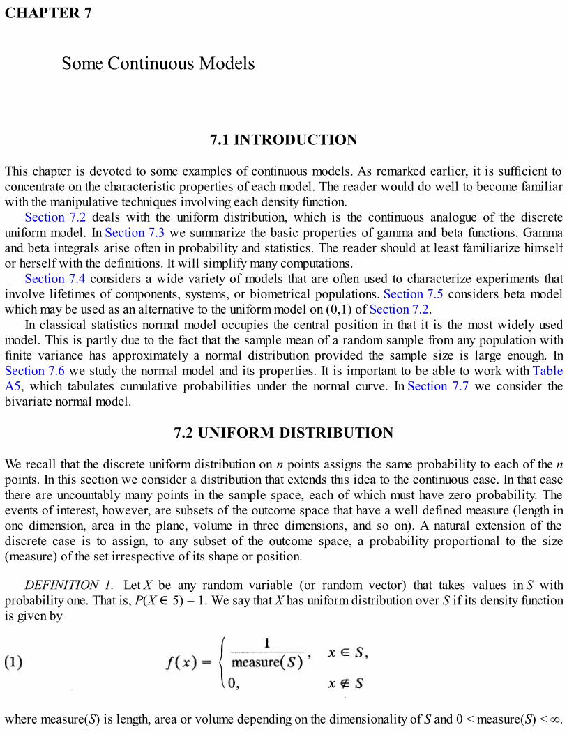
CHAPTER 7

Some Continuous Models

7.1 INTRODUCTION

This chapter is devoted to some examples of continuous models. As remarked earlier, it is sufficient toconcentrate on the characteristic properties of each model. The reader would do well to become familiarwith the manipulative techniques involving each density function.

Section 7.2 deals with the uniform distribution, which is the continuous analogue of the discreteuniform model. In Section 7.3 we summarize the basic properties of gamma and beta functions. Gammaand beta integrals arise often in probability and statistics. The reader should at least familiarize himselfor herself with the definitions. It will simplify many computations.

Section 7.4 considers a wide variety of models that are often used to characterize experiments thatinvolve lifetimes of components, systems, or biometrical populations. Section 7.5 considers beta modelwhich may be used as an alternative to the uniform model on (0,1) of Section 7.2.

In classical statistics normal model occupies the central position in that it is the most widely usedmodel. This is partly due to the fact that the sample mean of a random sample from any population withfinite variance has approximately a normal distribution provided the sample size is large enough. InSection 7.6 we study the normal model and its properties. It is important to be able to work with TableA5, which tabulates cumulative probabilities under the normal curve. In Section 7.7 we consider thebivariate normal model.

7.2 UNIFORM DISTRIBUTION

We recall that the discrete uniform distribution on n points assigns the same probability to each of the npoints. In this section we consider a distribution that extends this idea to the continuous case. In that casethere are uncountably many points in the sample space, each of which must have zero probability. Theevents of interest, however, are subsets of the outcome space that have a well defined measure (length inone dimension, area in the plane, volume in three dimensions, and so on). A natural extension of thediscrete case is to assign, to any subset of the outcome space, a probability proportional to the size(measure) of the set irrespective of its shape or position.

DEFINITION 1. Let X be any random variable (or random vector) that takes values in S withprobability one. That is, P(X ∈ 5) = 1. We say that X has uniform distribution over S if its density functionis given by

where measure(S) is length, area or volume depending on the dimensionality of S and 0 < measure(S) < ∞.

According to this definition, for any subset A of S that has a well-defined measure:

We shall be mostly interested in one or two dimensions.

Uniform Distribution on (a, b), – ∞ < a < b < ∞A random variable X has uniform distribution on (a, b) if its density function is given by

One may include either or both endpoints a and b.

Remark 1. We can now give yet another definition of “random.” A point is randomly chosen from Ssimply means that an observation is taken on a random variable X with density given by (1).

The uniform distribution is frequently used to model rounding-off errors in tabulating values to thenearest n decimal places. It is assumed that the error has uniform distribution on the interval [–10–n/2,10–n/2]. Similarly, the error in rounding off figures expressed in binary scale is assumed to have uniformdistribution on [–2–n, 2–n] or [0, 2–n], depending on how the rounding-off is done.

Example 1. Rounding-Off Error. Sales tax is rounded off to the nearest cent. Assuming that the actual error—the true tax minusthe rounded-off value—is random, that is, unsystematic, we can either use the discrete model

for j = –.005, –.004,…,0,.001,…,.005, or the simpler continuous model that the error X has density function

Example 2. Uniform Distribution in Plane. Suppose raindrops fall at random on a plane region S with area A(S). Let (X, Y) denotethe coordinates of the point in S where a particular raindrop strikes. Then (X, Y) has uniform distribution on S if the joint density is givenby:

In particular, if S is the unit square bounded by 0 ≤ x ≤ 1, 0 ≤ y ≤ 1, then A(S) = 1. If S is the triangle bounded by 0 ≤ y ≤ x ≤ 1 (or 0 ≤ x ≤y ≤ 1), then A(S) = , and so on (see Figure 1.). Since the probability that (X, Y) ∈ B ⊆ S is simply the volume of the solid with base Band height l/A(S), we need only compute the area of B either by integration or by using plane geometry. This observation greatly simplifiescomputation of probabilities under uniform distribution.

Let us now consider the uniform distribution on (a, b) with density function

Figure 1

Figure 2. Graphs of f and F given by (2) and (3).

Note that the distribution function corresponding to (2) is given by (see Figure 2):

Moreover,

In particular,

Mean and Variance of Uniform Distribition on (a, b)

We note that

where a ≤ c < d ≤ b so that the probability depends only on the length of (c, d) and not c and d. Thisproperty actually characterizes the uniform distribution.

Example 3*. A Characterizing Property of Uniform Distribution on (a, b). Let us rewrite (4) as follows:

and suppose that

If F has a continuous derivative f on (a, b) and satisfies (5) and (6), then F must be of the form (3). In fact, differentiating (5) werespect to x, we get

Since t is arbitrary it follows that f is constant on (a, b). Suppose f(x) = c for x ∈ (a, b). Then

and .

Problems of geometric probability can frequently be solved with ease by using uniform distribution.

Example 4. Choosing Two Points on (0, 1). Let X and Y be two points chosen (independently) at random from the interval (0,1).Find the probability that the three line-segments so formed form a triangle.

Since X and Y are independent, each with uniform distribution on (0,1), their joint density is given by

Now a necessary and sufficient condition for any three line-segments to form a triangle is that the sum of lengths of any two of them islarger than the length of the third. Hence we must have

The required probability can be obtained by integrating f over the two triangles. Since f is uniform on the unit square it is much easier tocompute the volume of the solid of unit height bounded by the two shaded triangles in Figure 3. It is sufficient to compute the area of theshaded triangles, and the required probability is .

Figure 3

Solution of any problem in geometric probability, however, depends on the definition of randomnessbeing used as illustrated in the following example.

Example 5. Bertrand’s Paradox. A chord is drawn at random in the unit circle. What is the probability that the chord is longer thanthe side of the equilateral triangle inscribed in the circle?

Let A be the event of interest. Then P(A) depends on the definition of randomness used.

Solution 1. The length of the chord is uniquely determined by the position of its midpoint. Choose a point C at random in the circle anddraw a line through C passing through the center of the circle O. Now draw the chord through C perpendicular to OC (see Figure 4a).Let l1 be the length of the chord through C. Then l1 > if and only if the point C lies inside the circle with center O and radius . It

follows that P(A) = Π(1/2)2/Π = . Here Ω is the circle with center O and a radius of one, so that

where C is the point (x, y).

Solution 2. In view of the symmetry of the circle, we choose and fix a point P on the circumference of the unit circle and take it to beone end point of the chord. The other end point P1 of the chord is now chosen at random. Thus Ω = [0, 2π) and

is the density of the length of the arc PP1. The inscribed equilateral triangle with P as one of its vertices divides the circumference of theunit circle into three equal parts. A chord through P will be longer than the side of this triangle if and only if P1 lies in that one-third part ofthe circumference which is opposite to P (see Figure 4b). It follows that P(A) = 1/3.

Figure 4

Solution 3. The length of the chord is uniquely determined by the distance of the midpoint of the chord from the center of the unitcircle. In view of the symmetry of the circle, assume that the midpoint P of the chord (see Figure 4c) lies on a fixed radius of the circle.Choose P at random so that the probability that P lies in any given segment equals the length of that segment. Thus Ω = [0, 1] and

where x denotes the distance of P from center O. The length of the chord will be longer than the length of the side of the inscribedequilateral triangle, if and only if x < 1/2. It follows that P(A) = 1/2.

Uniform distribution has important applications in nonparametric statistics and in simulation where itis used to generate random samples from a continuous distribution function F. These are taken up inSection 8.2 and later sections.

Problems for Section 7.2

1. The radius X of a ball bearing has uniform distribution over the interval (0, 1.5). Find:(i) P(X > .5), P(X < .4), P(.3 < X < 1.2).(ii) P{X > l.2|X > .5}.

2. The opening price of a particular stock on the New York Stock Exchange has uniform distribution on[35 1/8, 45 1/8].(i) Find the probability that the opening price is less than $40.(ii) What is the probability that the opening price is less than $44 given that it opened at a price

greater than $40?

3. Consider a computer storage system where the information is retrieved by entering the system at arandom point and systematically checking all the items in the system. Suppose it takes a seconds tobegin the search and b seconds to run through the entire system. Let X be the time it takes to search aparticular piece of information. Suppose b = ka, k > 1 fixed and P(X > 1) = lP(X < 1) for some l > 0.Find a.

4. A point X is chosen at random from the unit interval (0, 1). What is the probability that the area of therectangle formed by the two line-segments (from X to the two ends) is > 1/4? < 1/8?

5. Given that X has uniform distribution with mean c and variance d, 0 < d, find the density of X. Find theprobability that X > c + 1/2.

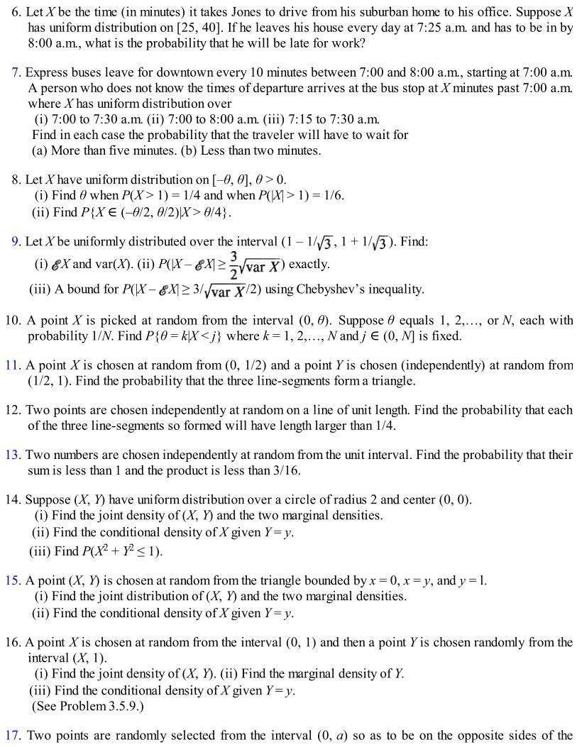
6. Let X be the time (in minutes) it takes Jones to drive from his suburban home to his office. Suppose Xhas uniform distribution on [25, 40]. If he leaves his house every day at 7:25 a.m. and has to be in by8:00 a.m., what is the probability that he will be late for work?

7. Express buses leave for downtown every 10 minutes between 7:00 and 8:00 a.m., starting at 7:00 a.m.A person who does not know the times of departure arrives at the bus stop at X minutes past 7:00 a.m.where X has uniform distribution over(i) 7:00 to 7:30 a.m. (ii) 7:00 to 8:00 a.m. (iii) 7:15 to 7:30 a.m.Find in each case the probability that the traveler will have to wait for(a) More than five minutes. (b) Less than two minutes.

8. Let X have uniform distribution on [–θ, θ], θ > 0.(i) Find θ when P(X > 1) = 1/4 and when P(|X| > 1) = 1/6.(ii) Find P{X ∈ (–θ/2, θ/2)|X > θ/4}.

9. Let X be uniformly distributed over the interval (1 – 1/ , 1 + 1/ ). Find:

(i) X and var(X). (ii) P(|X – X| ≥ ) exactly.

(iii) A bound for P(|X – X| ≥ 3/ /2) using Chebyshev’s inequality.

10. A point X is picked at random from the interval (0, θ). Suppose θ equals 1, 2,…, or N, each withprobability 1/N. Find P{θ = k|X < j} where k = 1, 2,…, N and j ∈ (0, N] is fixed.

11. A point X is chosen at random from (0, 1/2) and a point Y is chosen (independently) at random from(1/2, 1). Find the probability that the three line-segments form a triangle.

12. Two points are chosen independently at random on a line of unit length. Find the probability that eachof the three line-segments so formed will have length larger than 1/4.

13. Two numbers are chosen independently at random from the unit interval. Find the probability that theirsum is less than 1 and the product is less than 3/16.

14. Suppose (X, Y) have uniform distribution over a circle of radius 2 and center (0, 0).(i) Find the joint density of (X, Y) and the two marginal densities.(ii) Find the conditional density of X given Y = y.(iii) Find P(X2 + Y2 ≤ 1).

15. A point (X, Y) is chosen at random from the triangle bounded by x = 0, x = y, and y = l.(i) Find the joint distribution of (X, Y) and the two marginal densities.(ii) Find the conditional density of X given Y = y.

16. A point X is chosen at random from the interval (0, 1) and then a point Y is chosen randomly from theinterval (X, 1).(i) Find the joint density of (X, Y). (ii) Find the marginal density of Y.

(iii) Find the conditional density of X given Y = y.(See Problem 3.5.9.)

17. Two points are randomly selected from the interval (0, a) so as to be on the opposite sides of the

midpoint a/2. Find the probability that the distance between the two points is greater than a/3.

18. Let X, Y, Z be independent random variables each of which has a common uniform distribution on (0,1).

(i) Find P{0 ≤ X ≤ Y ≤ Z ≤ 1}. (ii) Find P{0 ≤ 3 Z ≤ 2 Y ≤ X ≤ 1}.

19. Let (X, y, Z) have uniform distribution over S = {(x, y, z): 0 ≤ x ≤ y ≤ z ≤ l}. Find(i) The joint density of (X, Y, Z).(ii) The marginal densities of X, Y and Z.(iii) The joint marginal densities of (X, Y), (Y, Z) and (X, Z).

20. Let X have uniform distribution on (0, 4). Find the probability that the roots of the quadratic equationx2 + 4xX + X + 1 = 0 are real.

21. Let X, Y, Z be independent random variables having common uniform distribution on (0, 1). Find theprobability that α2X + αY + Z = 0 has real roots.

7.3* GAMMA AND BETA FUNCTIONS

In many problems, the integrals

and

will be encountered. Let us first consider the integral in (1). The following result holds.

PROPOSITION 1. The integral converges or diverges according as α > 0 or ≤ 0. [For α > 0 the integral in(1) is called the gamma function and is denoted by Γ(α).]

Proof. We note that for as x → ∞. Hence for every ε > 0 there exists an x0 such

Let a > x0. Then for α > 0

Letting a → ∞ we have:

If, on the other hand, α ≤ 0, then for x < 1, xα ≥ 1 so that xα–1e–x ≥ e–x/x ≥ (xe)–1. It follows that for 0 < a < 1:

Letting a → 0 we see that cannot be finite for α ≤ 0.

A greater flexibility in choice of underlying distributions is achieved by introducing yet anotherparameter. We write x = y/β, β > 0 in

to get

Some simple properties of the gamma function are given below.

PROPOSITION 2. We have:

(i) Γ(α + 1) = αΓ(α) for α > 0,(ii) Γ(α + 1) = α! if α ≥ 0 is an integer, and(iii) Γ(1/2) = .

Proof. On integration by parts we have:

In particular, if α is integral then

To prove (iii) we change the variable by writing x = y2/2 in

to obtain

and it is sufficient to show that . Since

the integral is finite. Moreover,

Changing to polar coordinates by setting x = rcosθ and y = rsinθ, we have:

Consequently, I = and (iii) follows. We have also shown, in particular, that

is a density function.

Let us now consider the integral (2).

PROPOSITION 3. The integral converges for α > 0, β > 0 and is calledthe beta function. For α > 0, β > 0 we write

(For α ≤ 0 or β ≤ 0 the integral in (2) diverges.)

Proof. Let us write

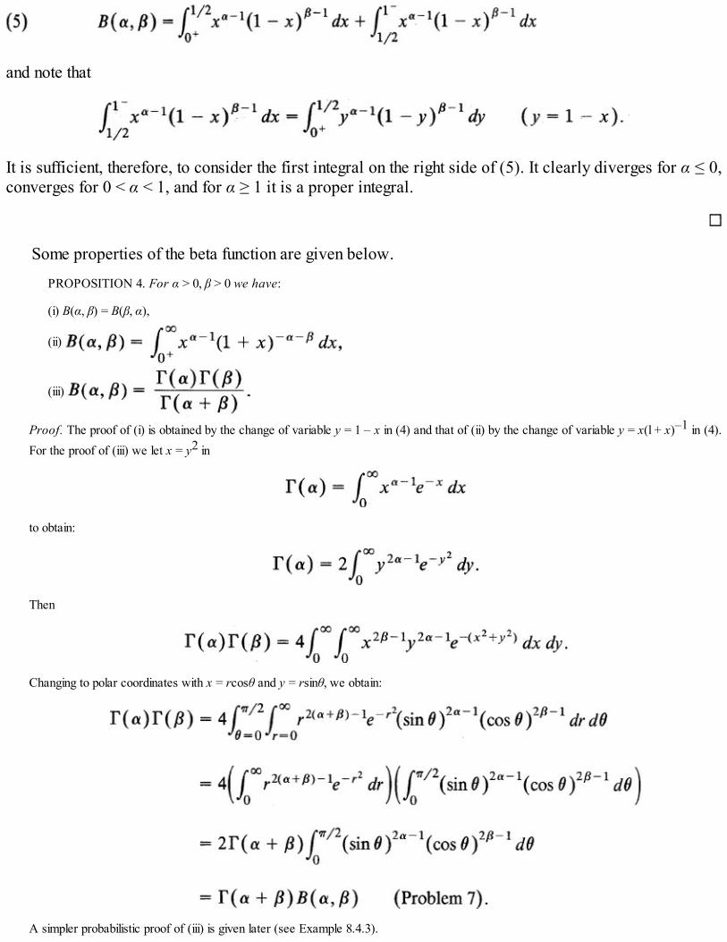
and note that

It is sufficient, therefore, to consider the first integral on the right side of (5). It clearly diverges for α ≤ 0,converges for 0 < α < 1, and for α ≥ 1 it is a proper integral.

Some properties of the beta function are given below.

PROPOSITION 4. For α > 0, β > 0 we have:

(i) B(α, β) = B(β, α),

(ii)

(iii)

Proof. The proof of (i) is obtained by the change of variable y = 1 – x in (4) and that of (ii) by the change of variable y = x(l + x)–1 in (4).For the proof of (iii) we let x = y2 in

to obtain:

Then

Changing to polar coordinates with x = rcosθ and y = rsinθ, we obtain:

A simpler probabilistic proof of (iii) is given later (see Example 8.4.3).

For convenience, we write:

It will always be clear from the context what the limits of integration are. We conclude this section withthe following application of gamma functions.

PROPOSITION 5. (STIRLING’S APPROXIMATION). For sufficiently large n

Proof. We will sacrifice rigor by proceeding informally. We have

The function n ln x – x has a relative maximum at x = n. We therefore substitute x = n + y on the right side of (7) to obtain

Let us now use Taylor expansion for ln(l + y/n) to obtain

Hence for large n, we get:

in view of the fact that

[see proof of Proposition 2(iii)].

Problems for Section 7.3

1. Compute Γ(3/2), Γ(9/2), Γ(4), Γ(10).

2. Compute .

3. Compute .

4. Compute

5. Compute

6. Compute .

7. Show that . [Hint: Substitute x = sin2y in (4).]

8. Show that .

9. Compute

10. Let n be an odd positive integer. Show that

11. Show that for α > 0:

Use (ii) to derive .

Use (iii) to show that for nonnegative integral n and σ > 0

(This last result essentially gives the moments of normal distribution with mean 0 and variance σ2. See Section 7.6.)

12. Use Proposition 4 parts (ii) and (iii) for α = β = to prove Proposition 2 (iii).

7.4 EXPONENTIAL, GAMMA, AND WEIBULL DISTRIBUTIONS

We recall that the distribution of the number of trials needed for the first success in a sequence ofBernoulli trials is geometric. A continuous analogue of this result is very useful in modeling life length (oforganisms or pieces of equipment). Consider a sequence of events that occur randomly in time accordingto the Poisson distribution at rate λ > 0. In Section 6.6 we derived the distribution of the number of eventsX(t) in the interval [0, t]. Suppose we now ask for the distribution of the waiting time for the first(Poissonian) event. Let T denote this random variable. Then

and the density of T is given by

The density function defined in (1) is called an exponential density function. The distribution function isgiven by

We note that f is strictly decreasing with unique mode at t = 0 where f takes the value λ. The median of fis at t = (In 2)/λ and t-axis is in asymptote of f. The distribution function F rises steadily from zero at t = 0to one at t = ∞[F(t) = 1 is an asymptote]. Figure 1 gives sketches of f and λ for λ = 1.

The moments of T are easily computed. Indeed, for α > 0:

Hence

It will be convenient to write λ for 1/λ.

Exponential Density Function

Figure 1. Graphs of f and F.

Example 1. Memoryless Property of Exponential Distributions. An interesting property is characteristic of the exponentialdistribution. Let s, t ≥ 0. Then

If we think of T as lifetime of a piece of equipment, then (3) states that if the equipment has been working for time s then the probabilitythat it will survive an additional time t depends only on t and equals the probability of survival for time t of a new piece of equipment. Thusthe equipment does not “remember” that it has been in use for time s. In this sense there has been no deterioration. We recall thatproperty (3) holds also for geometric random variables and just as (3) characterizes geometric distribution it also characterizes theexponential distribution in the sense that if, for a continuous nonnegative random variable T

holds for all s, t ≥ 0 then T must have an exponential distribution.The lack of memory property simplifies many calculations and is precisely the reason for wide applicability of the exponential model. It

should be understood that under this model an item that has not failed is as good as new, so that the operating time of the item may beidentified with operating age. This is certainly not the case for any other (nonnegative continuous type) random variable. The conditionalprobability

depends on s (except when T is exponentially distributed) so that T here is the total length of life rather than the time in service (as in theexponential case).

Example 2. Waiting Time at a Restaurant. Suppose that the amount of time a customer spends at a fast food restaurant has anexponential distribution with a mean of six minutes. Then the probability that a randomly selected customer will spend more than 12minutes in the restaurant is given by

whereas the (conditional) probability that the customer will spend more than 12 minutes in the restaurant given that she has been there formore than six minutes is

Example 3. Life Length of a Water Heater. Suppose that the life length of a water heater produced by a certain company has anexponential distribution with mean 12 years. Mrs. Tennenbaum buys an old house with this brand of water heater. She would like to sellthe house in four years. What is the probability that she will not have to replace the water heater before she sells?

In view of the lack of memory property, the remaining lifetime of the water heater has an exponential distribution with mean 12 years.

Indeed, if T is the life length of the water heater then

This computation would not be possible for any other lifetime distribution F since in that case we need to know time t, the prior use of thewater heater.

Weibull and Gamma Distributions*

Frequently in life testing the representation by an exponential model is not adequate. An electriccomponent subjected to continuous vibrations or a steel beam under continuous stress will deteriorateover time so that an exponential model to describe the distribution of length of life in such cases will notbe adequate. We now consider some modifications of the exponential model that allow greater flexibility.The following examples will help motivate our discussion.

Example 4. Waiting Time for the rth Customer. In the beginning of Section 7.4 we showed that the distribution of the waiting timeof the first event in a sequence of events occurring randomly in time according to the Poisson law is exponential. Frequently we areinterested in the distribution of the waiting time for the rth occurrence.

Suppose customers arrive at a service desk (automobiles at a toll booth or calls into an exchange) according to the Poisson law atmean rate λ per unit time. Let Tr be the time of occurrence of the rth event and let

Then

where X(t) = number of events in time [0, t]. Since X(t) has Poisson distribution with X(t) = t/λ (Why?), we have

so that for t ≥ 0

and

gives the density function of Tr. We note that fr(t) is a gamma function with α = r and β = λ except that r is an integer, r ≥ 1, and r = 1

gives the exponential distribution (with mean λ).

Example 5. Survival Analysis. To model the length of life T of a living organism or a system or a component, it is a more convenientto consider the survival function:

where F is the distribution function of T with density function f. Yet another function plays a key role in survival analysis. This is thehazard (failure rate) function X(t), defined by

for S(t) > 0. The function λ(t) may be interpreted as the conditional probability density that a t-year old component will fail. Indeed, for Δtsmall

We note that λ(t) uniquely determines f. For,

so that if F(0) = 0, then

Hence

Suppose for fixed λ > 0,

Then

and

That is, an exponential density function is the only distribution with constant failure rate. In some situations λ(t) = constant is not areasonable assumption. A modification is obtained if we assume instead that the failure rate associated with T is of the form

Then (6) yields the density

A random variable with density function (8) is said to have a Weibull distribution. We note that α = 1, β = λ in (8) yields the exponentiallaw with mean λ. A special case of (8) with α = 2 is the Rayleigh density function

which has linear hazard rate λ(t) = 2t/β. Actually, Weibull law is closely related to the exponential law. Indeed

so that if T1 is Weibull with density (8) and T2 is exponential with mean β, then

The distributions encountered in Examples 4 and 5 and many more are simply related to (or arespecial cases of) the gamma probability density function with parameters α > 0, β > 0, given by

In view of (7.3.3), we note that (10) does indeed define a density function.The gamma density function takes on a wide variety of shapes depending on the values of α and β. For

α < 1, f is strictly decreasing and f(x) → 0 as x → ∞, f(x) → ∞ as x → 0. For α > 1, the density f has aunique mode at x = (α – 1)β with maximum value . Figure 2 gives graphsof some typical gamma probability density functions.

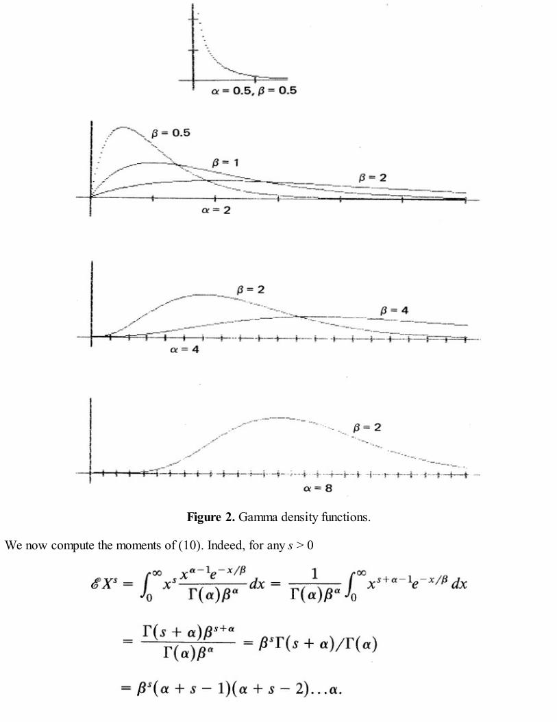
Figure 2. Gamma density functions.

We now compute the moments of (10). Indeed, for any s > 0

In particular

Mean and Variance of Gamma Density

Example 6. Peak Signal Strength. The peak signal X (in volts) arriving at an antenna has a Weibull (or Rayleigh) distribution withparameters α = 2 and β so that the density function of X is given by

Then for t > 0

so that for s, t > 0

which depends on t as well as s. In particular, if s, t are known and P{X > s + t|X > t} = γ, 0 < γ < l, is also known, then β is given by

so that

Some important special cases of gamma distribution are widely used and have been given special names. Letting α = 1 in (10) gives anexponential density with mean β. Letting α = n/2 and β = 2σ2 in (10) yields a σ2χ2 (σ2 chi-square) density with n degrees of freedom(d.f.) given by

Here the parameter n takes positive integral values and parameter α > 0. If we take α = 1 in (12) we get the well known chi-square (χ2)density

with n d.f. Since f in (12) is a density function, we have

and it follows that the function

also defines a density function. It is called a σχ density with parameters n = 1,2,… and σ > 0. The special case σ = 1 is known as a χdistribution with n degree of freedom. Some special cases of (14) are widely in use.

Rayleigh distribution with density function

is the special case n = 2 and σ = α . (This is the density (9) with β = 2α2.)

Figure 3. χ density for n = 2, 3, 5, 10.

Maxwell density function

is the special case n = 3 and σ = α .

Weibull distribution (8) is also obtainable from (12) by substituting n = 2, σ2 = β, and the change ofvariable x = 2tα. Figures 3 and 4 give graphs of chi and Weibull densities.

Example 7. Weekly Consumer Demand for Bread Suppose the weekly consumer demand X for bread in a certain town has agamma distribution with parameters α and β. What is the probability that the demand for bread in a certain week in this town will begreater than t? What we need to do is to compute the survival function P(X > t) of X. We have:

Given t, α, β one can look up the probability in a table of incomplete gamma function.

Figure 4. Weibull density.

There is yet another way to look at this probability. In Example 4 we showed that for a gamma random variable with parameters α = rand β > 0 where r ≥ 1 is an integer

Hence in the special case when α is a positive integer, we can find P(X < t) from a table of cumulative Poisson distribution function (suchas Table A4) with parameter λ = t/β.

In particular, if α = 12, β = 3 and t = 48 then

Problems for Section 7.4

Problems 11 to 25 refer to the Subsection on gamma distribution.

1. The times between successive arrivals of customers in a store are governed by the density function

(i) Find the probability that a customer arrives after time t.(ii) Find the probability that a customer arrives after time tl but not after time t2, 0 < t1 < t2.

2. On the Boston–Chicago route, the number of minutes a plane is late is an exponential random variable with a mean of 10 minutes. Find theprobability that the flight will be late by more than 10 minutes on a randomly selected day. Show that your result is independent of themean of the exponential distribution. That is, show that P(X > X) is independent of X = λ.

3. Let X measure the time to failure (in hours) of a car battery of a certain brand. Suppose X has exponential distribution with mean λ. If nsuch batteries are installed and operate independently, what is the probability that one-half or more of them are still functioning at the endof t hours? In particular, if X = 200 and t = 100 hours, find the probability that 16 or more of the batteries are still functioning out of the25 batteries installed.

4. (i) If X has exponential distribution with mean, λ, find c such that P(X > c) = α, 0 < α < 1.(ii) Find c1 and c2 such that P(c1 < X < c2) = β and P(X < c1) = γ; β, γ > 0, 0 < β + γ < 1.(iii) Find P(X < –λ ln(l – p)) for 0 < p < 1.

5. Three processes are used to produce fuses for electrical circuits. Process 1 yields a mean life length of 100 hours, process 2 has anexpected life length of 150 hours, and Process 3 yields an expected life of 200 hours. Suppose Process 1 costs $c per unit, Process 2 costs$(3/2) c per unit, and Process 3 costs $2c per unit. Moreover, if a fuse lasts for less than 200 hours there is an assessment of $d againstthe manufacturer. Find the expected cost of producing a fuse in each case. Assume that the life length has an exponential distribution.

6. An electronic device has a life length X (in 1000 hour units). Suppose X has an exponential density function with mean 1. Suppose furtherthat the cost of manufacturing an item is $2.50 and the proceeds from the sale of one unit is $3. If the item is guaranteed a refund, if itdoes not survive 100 hours, what is the manufacturer’s expected profit per item?

7. Let X have an exponential distribution with parameter λ > 0. Find P(k < X ≤ k + 1), k ≥ 0 integral, and show that it is of the form p(1 –p)k . Find p.

8. Suppose that a car battery has life length X (hours) which has an exponential distribution with mean λ. A machine using this battery costs$k1 per hour to run, and while the machine is functioning a profit of $k2 per hour is realized. Suppose that this machine needs an operatorto run it and the operator is paid $T per hour. If the operator is hired for t hours, find:

(i) The expected profit.(ii) The minimum number of hours t for which the expected profit is maximized.

9. The compressor of a new heat pump is guaranteed for 5 years. The mean life is estimated to be 6 years and the time to failure can beassumed to be exponential. If each failure of the compressor costs $50 and the realized profit on each heat pump is $700, what is theexpected profit per heat pump? (Hint: The number of failures in [0, t] has a Poisson distribution with λ = t/6.)

10. Suppose X has an exponential distribution with a mean of λ > 0. Compare the upper bound on the probability P(|X – μ| ≥ 2σ) obtained fromChebyshev’s inequality with the exact probability. [Here μ = X = λ and σ2 = var(X) = λ2.]

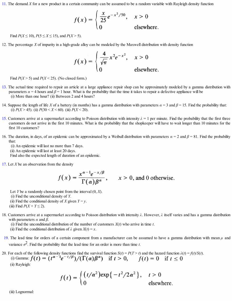
11. The demand X for a new product in a certain community can be assumed to be a random variable with Rayleigh density function

Find P(X ≤ 10), P(5 ≤ X ≤ 15), and P(X > 5).

12. The percentage X of impurity in a high-grade alloy can be modeled by the Maxwell distribution with density function

Find P(X > 5) and P(X < 25). (No closed form.)

13. The actual time required to repair an article at a large appliance repair shop can be approximately modeled by a gamma distribution withparameters α = 4 hours and β = 1 hour. What is the probability that the time it takes to repair a defective appliance will be

(i) More than one hour? (ii) Between 2 and 4 hours?

14. Suppose the length of life X of a battery (in months) has a gamma distribution with parameters α = 3 and β = 15. Find the probability that:(i) P(X > 45). (ii) P(30 < X < 60). (iii) P(X < 20).

15. Customers arrive at a supermarket according to Poisson distribution with intensity λ = 1 per minute. Find the probability that the first threecustomers do not arrive in the first 10 minutes. What is the probability that the shopkeeper will have to wait longer than 10 minutes for thefirst 10 customers?

16. The duration, in days, of an epidemic can be approximated by a Weibull distribution with parameters α = 2 and β = 81. Find the probabilitythat:

(i) An epidemic will last no more than 7 days.(ii) An epidemic will last at least 20 days.Find also the expected length of duration of an epidemic.

17. Let X be an observation from the density

Let Y be a randomly chosen point from the interval (0, X).(i) Find the unconditional density of Y.(ii) Find the conditional density of X given Y = y.(iii) Find P(X + Y ≤ 2).

18. Customers arrive at a supermarket according to Poisson distribution with intensity λ. However, λ itself varies and has a gamma distributionwith parameters α and β.

(i) Find the unconditional distribution of the number of customers X(t) who arrive in time t.(ii) Find the conditional distribution of λ given X(t) = x.

19. The lead time for orders of a certain component from a manufacturer can be assumed to have a gamma distribution with mean μ andvariance σ2. Find the probability that the lead time for an order is more than time t.

20. For each of the following density functions find the survival function S(t) = P(T > t) and the hazard function λ(t) = f(t)/S(t).(i) Gamma: (ii) Rayleigh:

(iii) Lognormal:

(iv) Pareto: f(t) = αaα/tα + 1 for t > a, and 0 elsewhere.

21. If the hazard rate λ(t) for a density f is increasing, we say that f has an increasing failure rate. Similarly we can define decreasingfailure rate. Show that the results in the following table hold.

Failure RateConstant Increasing DecreasingExponential Weibull (α > 1) Weibull (α < 1)

Gamma (α > 1) Gamma (α < 1)Rayleigh (α ≠ 0) Pareto (t > a)

22. For the gamma density function show that limt→∞λ(t) = 1/β.

23. Show that for the Weibull density

the mean and the variance are given by

24. Find the mean and the variance of a σ chi distribution with density

and hence also for Rayleigh and Maxwell densities.

25. For the Pareto density function f(t) = αaα/tα + 1, for t > a and f(t) = 0 if t ≤ a, find the mean and the variance whenever they exist.

7.5* BETA DISTRIBUTION

We now introduce another distribution on (0,1) which can be used to model distribution of proportionsand which provides greater flexibility than the uni-, form distribution on (0,1). In Section 7.3 we defineda beta function by the integral

where α, β > 0. The integrand in (1) is nonnegative on (0, 1), and in view of (1)the function

defines a density function. The density function in (2) is known as a beta density function withparameters α and β. The special case α = β = 1 yields the uniform distribution on (0,1).

In order to graph a beta probability density function, we note that if α > 1, β > 1 then f(x) → 0 as x →0 or x → 1. If 0 < α < 1 then f(x) → ∞ as x → 0, and if 0 < β < 1 then f(x) → ∞ as x → 1. For α > 1 and β> 1, f has a unique mode at x = (α – 1)/(α + β – 2); for α < 1 and β > 1, f has a unique minimum at x = (α –l)/(α + β – 2), so that the density is U-shaped. In the special case when α = β, the density is symmetricabout the median x = 1/2. Figure 1 gives graphs of several beta probability density functions.

For any r > 0 we have

Figure 1. Beta density for (α, β) = (1, 2), (2, 2), (4, 2), (8, 2) and (9, 2), (4, 4) and (.5, .5).

Now recall that B(α, β) = Γ(α)Γ(β)/Γ(α + β).Hence:

In particular,

Beta density function arises naturally in sampling from a normal population and also as thedistribution of order statistics in sampling from a uniform distribution. In Bayesian statistics (see Sections10.6 and 10.7) it is a preferred prior for the parameter p of a binomial distribution.

Example 1. Proportion of Erroneous Income Tax Returns. Suppose that the proportion X of erroneous income tax returns filedwith the Internal Revenue Service each year can be viewed as a beta random variable with parameters α and β.

The probability that in a randomly chosen year there will be at most 100γ percent erroneous returns is

In particular, if α = 2 and β = 12 then

If γ = .1 then P(X ≤ Y) = 1 – 2.2(.9)12 = .3787.

In some cases, there is a simpler way to compute probabilities such as P(X < γ) under betadistribution. One can use the binomial tables.

Example 2. Relation Between Beta and Binomial Distributions. Suppose X has a beta distribution with parameters α and β and let0 < p < 1. Then

Suppose both α and β are positive integers. Then we can rewrite (5) as

Integrating by parts (α – 1) times we see that

where Y is a binomial random variable with parameters α + β – 1 and p. For convenience write α + β = n + 1 and α = k . Then we have(see also Problem 6.3.22)

Relation Between Beta and Binomial

In Example 1, p = .1 and α = 2, β = 12 so that n = 13, k = 2 and

where Y is binomial with n = 13, p = .1. From Table A3:

Yet another application is the following. Let Y1 Y2 be binomial with parameters n, pl and n, p2respectively. Then p2 > P1 implies

and it follows that

Alternatively, we can write

Thus if p2 > p1 then Y2 has more probability in the right tail than Y1 does; that is, the larger the p the moreshifted the distribution to the right.

Problems for Section 7.5

1. Let X be a random variable with beta density function with parameters α and β. In each of thefollowing cases verify that the beta density integrates to one:

(i) α = 1 and β = 8. (ii) α = 2 and β = 4. (iii) α = 3 and β = 4.

2. The proportion of defective television tubes made by some company has a beta distribution with α = 2and β = 3.

(i) What is the average proportion of defective tubes that this company makes?(ii) Find the probability that the proportion of defective tubes will be between .2 and .5.

3. The annual proportion of new gas stations that fail in a city may be considered as a beta randomvariable with α = 2 and β = 10.

(i) Find the average annual proportion of new gas stations that fail in this city.(ii) Find the probability that 20 percent or more of all new gas stations will fail in any one year.(iii) Find the probability that between 5 and 10 percent of new gas stations will fail in a year.

4. The relative humidity measured at a certain location can be thought of as a random variable withdensity function

(i) Find c.(ii) Find the probability that the relative humidity at this location will be at least 35 percent.

5. The percentage of tires per lot manufactured by a certain company has a beta distribution with α = 2and β = 6. It is known that any lot containing more than 25 percent defective tires will have to be soldas blemished. What is the probability that a randomly selected lot will be sold as blemished?

6. The proportion of blood-spotted eggs laid by hens in a flock may be considered a beta randomvariable with parameters λ = 3 and β = 11. Find the probability that

(i) The proportion of blood-spotted eggs on a given day is between .05 and .15.(ii) The proportion is larger than the mean proportion.

7. Let X have a beta distribution with mean μ and variance σ2. Find α and β. In particular, find α and βwhen μ = .1, σ2 = .05.

8. It is known that for a beta random variable X with parameters α and β P(X < .2) = .22. If α + β = 26,find α and β. (Hint: Use Binomial Table A3.)

9. The proportion of patients who respond favorably to a new drug is known to have a beta distributionwith parameters α and β. Let X be the number of patients who show improvement out of a randomlyselected n patients all of whom were administered the new drug. Find the unconditional distributionof X. Find the conditional distribution of the proportion of patients who respond favorably to the newdrug given X = k.

10. The proportion of patients who respond favorably to a new drug is known to have a beta distributionwith parameters α and β. Randomly selected patients are administered the new drug and are testedsequentially. Let X be the number of patients needed to get r patients who respond favorably. Find theunconditional distribution of X, its mean and variance. Find also the conditional distribution of theproportion of favorable responses given X = k + r, k = 0, 1, 2….

11. Let X have beta distribution with parameters α and β. Find {Xp(l – X)q}.

7.6 NORMAL DISTRIBUTION

The normal distribution has a well deserved claim to be the most commonly used distribution in statistics.Part of the reason is the central limit theorem (Section 9.3) which essentially says that in random samplingfrom a population with finite variance the sample mean has a distribution that looks more and more likenormal distribution as the sample size increases. In this section we consider some useful properties of thenormal distribution.

A random variable X is said to have a normal distribution with parameters μ and σ2 if its densityfunction is given by

We will show that μ = X and σ2 = var(X). In particular, if μ = 0 and σ = 1, we say that X has a standardnormal distribution. (We write Z for a standard normal random variable.)

We first check that (1) does indeed define a density function. In fact, f(x) > 0 for x ∈ and

in view of Proposition 7.3.2(iii). We will use this fact often, and we restate it for emphasis. Let a ∈ and b > 0. Then:

Let us next compute the mean and the variance of X. We have

Here the first integral vanishes since the integrand is an odd function and the second integral equals one inview of (2). Next we have

Normal Probability Density Function

Special case μ = 0, σ = 1: standard normal.

To graph a normal density with mean μ and variable σ2, we note that the density is symmetric about μ.That is,

Moreover, f has a maximum at x = μ with maximum value f(μ) = 1/(σ ). As |x| → ∞, f(x) → 0. Thus fis unimodal, and mean, median, and mode coincide at x = μ. Graphs of several normal distributions aregiven in Figure 1.

Figure 1. Normal density for μ = 0 and σ = 1, 2, 3.

In view of the great importance of normal distribution, the distribution function of a standard normalrandom variable Z has been tabulated extensively. Table A5 in the Appendix gives the probability P(0 <Z < z) (see Figure 2) for values of z = .00(.01)3.09. Probabilities corresponding to negative values of zcan be obtained by symmetry. Thus, for z > 0:

How do we use Table A5 when μ ≠ 0 and/or σ ≠ 1? We standardize X That is, suppose we want P(X≤ c) for a normal random variable with mean μ and

Figure 2. P(0 < Z < z) under standard normal.

variance σ2. Then on standardizing X we get

where Z is standard normal. This is so because

An alternative way to look at P(X ≤ c) is as follows. Table A5 gives the probability that the (standard)normal variable Z will be within z standard deviation units of the mean. To find P(X ≤ c) we need to findthe number of standard deviation units that c is from the mean μ. Since

we see that c is (c – μ)/σ standard deviation units from μ. Hence P(X ≤ c) = P(Z ≤ (c – μ)/σ).

Example 1. How Good Is Chebyshev’s Bound? We recall that for a random variable X with mean μ and variance σ2

for k > 1. If, however, X is normal, then

Table 1 shows that almost all the probability under a normal distribution is assigned to the interval (μ – 3σ, μ + 3σ) even though f(x)never touches the x-axis. Chebyshev’s inequality always underestimates the exact probability.

TABLE 1. Comparison of Chebyshev Bounds and Exact Probabilities , P(|X – μ| ≤ kσ).

k Chebyshev Bound (≥) Exact Probability1.0 0 .68261.5 .5556 .70622.0 .75 .95442.5 .84 .98763.0 .8889 .99743.5 .9184 .9978

Example 2. Finding Probabilities Under Normal Curve. Let Z be a standard normal random variable. Then, from Figure 3 andTable A5:

and

Suppose we want to find z such that P(Z > z) = .05 or P(|Z| > z) = .02. To find P(Z > z) = .05 we note from Figure 4 that z mustsatisfy P(0 < Z < z) = .45. From Table A5 we see that z = 1.645. To find z with P(|Z| > z) = .02 we note from Figure

Figure 3

Figure 4

4 that z must satisfy P(Z > z) = .01 by symmetry so that P(0 < Z < z) = .49. Hence from Table A5 we have z = 2.33.

In statistics, tail probabilities under the normal curve have special significance. For that reason wewill use the notation zα, for 0 < α < 1, to denote the quantile of order 1 – α. That is

In Table 2 we list some commonly used values of α and zα.

Example 3. Distribution of Ages of Workers. The ages of workers in a large plant have a normal distribution with mean age 40years and standard deviation 7 years. Let

TABLE 2. Tail Probabilities Under Normal Distribution

α zα/2 zα.01 2.575 2.33.02 2.33 2.05.05 1.96 1.645.10 1.645 1.28

X be the age of a randomly selected worker. Then X has a normal distribution with μ = 40, σ = 7. The reader may wonder how X can

have a normal distribution. Does not a normal random variable take negative values? The answer is that almost all of the probability isassigned to the interval (μ – 3σ, μ + 3σ), as seen in Example 1. In fact,

The proportion of workers aged between 50 and 60 is given by

The proportion of workers aged 35 years or younger is given by

Let us find the age x below which are 20 percent of the workers. We want to find x such that

Clearly, x < μ, (see Figure 5). Also:

From Table A5, (x – 40)/7 = –.84 so that x = 34.12. Alternatively, we note from

Figure 5

Table A5 that .2995 ( .30) of the area under the normal curve is between μ and μ – .84σ. It follows that if x is located at –.84σ distancefrom μ, then about .20 proportion of the workers will be younger than age x. Hence

Example 4. Grades and Normal Distribution. The grades in a large section of a calculus course are approximately normally

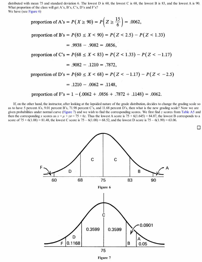
distributed with mean 75 and standard deviation 6. The lowest D is 60, the lowest C is 68, the lowest B is 83, and the lowest A is 90.What proportion of the class will get A’s, B’s, C’s, D’s and F’s?We have (see Figure 6)

If, on the other hand, the instructor, after looking at the lopsided nature of the grade distribution, decides to change the grading scale soas to have 5 percent A’s, 9.01 percent B’s, 71.98 percent C’s, and 11.68 percent D’s, then what is the new grading scale? Now we aregiven probabilities under normal curve (Figure 7) and we wish to find the corresponding scores. We first find z scores from Table A5 andthen the corresponding x scores as x = μ + zσ = 75 + 6z. Thus the lowest A score is 75 + 6(1.645) = 84.87, the lowest B corresponds to ascore of 75 + 6(1.08) = 81.48, the lowest C score is 75 – 6(1.08) = 68.52, and the lowest D score is 75 – 6(1.99) = 63.06.

Figure 6

Figure 7

Example 5. Standard Deviation Setting of a Coffee Vending Machine . A coffee vending machine dispenses 6 ounces of coffeeper cup, on the average. Assuming that the amount dispensed is normally distributed, at what level should the standard deviation be set sothat 98 percent of the cups will have at least 5.85 ounces of coffee?

Since 98 percent of the cups will have at least 5.85 ounces of coffee (Figure 8), it follows from Table A5 that 5.85 is 2.05σ smallerthan μ. Thus,

and it follows that σ = .15/2.05 = 0.0732.If the cups can hold at most 6.1 ounces of coffee, the proportion of those that will spill over is given by

As mentioned earlier, normal distribution arises often in practice. For example, according toMaxwell’s law in physics the components of velocity of a molecule of mass m in a gas at absolutetemperature T has a normal distribution with mean 0 and variance σ2 = m/(kT) where k is a physicalconstant. Frequently, though, normal distribution is only an approximation to the random phenomenonunder

Figure 8

study. Thus when we say that height of a group of individuals obeys a normal law it simply means that thedistribution is symmetric and bell-shaped and may be approximated by a normal distribution. Othertypical examples include distribution of weights of a biometrical population, distribution of errors ofmeasurements in physical experiments, distribution of scores on the Graduate Record Examination,distribution of certain lengths of life, distribution of output from a production line, and so on. If thepopulation is heterogeneous, one needs to be careful. Thus the distribution of heights of teenagers aged15–18 may be bimodal and hence not normal since it includes both boys and girls. The two distributionsseparately are approximately normal. Similarly the distribution of incomes of a large heterogeneous groupis not likely to be normal. Later on (Section 9.3), we will study the central limit theorem and see that thedistribution of sample averages is frequently approximately normal when the sample size is large.

Problems for Section 7.6

1. For a standard normal random variable Z find(i) P(Z ≤ .54). (ii) P(Z > .27). (iii) P(|Z| ≤ 1.63).(iv) P(–.64 < Z < 1.29). (v) P(.69 < Z < 2.37).(vi) P(.45 < |Z| < 1.96). (vii) P(Z < –.86).

2. Let Z be a standard normal random variable. Find c such that:(i) P(Z ≤ c) = .1772. (ii) P(Z ≥ c) = .0068.

(iii) P(Z ≥ –c) = .0044. (iv) P(|Z| ≥ c) = .05.(v) P(Z ≤ c) = .9564. (vi) P(|Z| ≤ c) = .90.

3. Let X have a normal distribution with mean 7 and variance 9. Find:(i) P(X > 8). (ii) P(X > 5). (iii) P(4 < X < 9).(iv) P(X < 3 or X > 7.5). (v) P(|X| > 5). (vi) P(|X| < 8).

4. Suppose X has a normal distribution with mean 1 and variance 4. Find:(i) P(X = 1). (ii) P(X ≥ 0). (iii) P(–l < X < 0.5).(iv) P(|X| < 2). (v) P(|X| > 1.5). (vi) P(X > 6.5).

5. Let X have a normal distribution with mean μ, and standard deviation σ. Find x such that(i) P(X ≥ x) = .95, if μ = 1, σ = 2.(ii) P(X ≥ x) = .0068, if μ, = 6, σ = 3.(iii) P(x < X < 1.40) = .2712, if μ = 0, σ = 1.(iv) P(X > x) = 3P(X ≤ x), if μ = 2, σ = 3.(v) P(|X| > x) = .0076, if μ = 0, σ = 1.(vi) P(|X – μ| ≤ x) = .9660, if μ = 50, σ = 10.

(vii) P(|X| > x) = P(|X| ≤ x), if μ = 0, σ = 1.

6. For what values of c are the following functions density functions? In each case find thecorresponding mean and the variance.

(i) f(x) = (c/ )exp(–x2 + x), x ∈ .(ii) f(x) = cexp(–5x2 + 9x – 11), x ∈ .(iii) f(x) = (1/ )exp(–x2 + x – c), x ∈ .(iv) f(x) = exp{–cx2 – x – 4}, x ∈ .

7. The final examination scores in a large class on Principles of Economics are normally distributedwith a mean score of 60 and a standard deviation of 10.

(i) If the lowest passing score is 48, what proportion of the class is failing?(ii) If the highest 80 percent of the class is to pass, what is the lowest passing score?

8. The diameter of a large shipment of ball bearings has a normal distribution with mean 2 cm andstandard deviation 0.01 cm.

(i) What is the proportion of ball bearings from this shipment that have a diameter larger than 2.02cm?

(ii) Suppose ball bearings with diameter larger than 2.02 cm or smaller than 1.98 cm areunacceptable. If a random sample of three ball bearings is selected, what is the probability thatexactly two of them will be unacceptable?

9. A certain machine makes iron rods with a diameter of 0.5 cm. Because various factors influence aproduction process, however, the diameter is .505 + .01Z where Z is a standard normal randomvariable. What is the probability that a given iron rod produced by this machine will have a diameterthat will be within .01 cm of the nominal diameter?

10. Optimum mean weight for a particular height and body frame for males can be assumed to have anormal distribution with a mean of 126 pounds and a standard deviation of 5 pounds. Suppose a malewith weight 2.5 standard deviation above the mean is considered to be obese.

What is the proportion of males of this particular height and body frame who are obese? Is aweight of 138 pounds obese? In a sample of 15 such males what is the probability that at least onewill be obese?

11. Suppose the systolic blood pressure for normal males is a normal random variable with mean 120 mmHg and standard deviation 20 mm Hg. If a person with blood pressure 2.5σ above the mean isconsidered hypertensive and to be referred for further diagnosis, what proportion of males fall in thiscategory? How many males have a blood pressure below 100 mm Hg. and above 160 mm Hg? Howwould you classify a reading of 180 mm Hg?

12. The birth weight of girls in the United States is a normal random variable with a mean of 7.41 poundsand a standard deviation of 2 pounds. How probable is a birth weight of 3 pounds or less or 11pounds or more? If a birth weight of 12 pounds is considered overweight, what proportion of newlyborn infant girls are overweight?

13. The scores of students taking the verbal portion of the Graduate Record Examination are artificiallystandardized to have mean score 500 and standard deviation 100.(i) If your sister scored 654, what percentage of students taking the test ranked higher?(ii) If your brother scored 540, what is his percentile rank?(iii) What score qualifies a student for the top 10 percent of all candidates?(iv) The top 5 percent?

14. The heights of male freshmen entering a large state university are normally distributed with a mean of68 inches. It is known that about 5 percent of the freshmen are taller than 72 inches.(i) What is the standard deviation of the distribution of heights?(ii) What is the proportion of the freshmen males at this college who have a height of 63 inches or

less?

15. The weights of instant coffee jars packed by a food processor are normally distributed with a standarddeviation of .2 ounce. The processor has set the mean such that about two percent of the jars weighmore than 8.41 ounces. What is the mean setting?

16. The pebbles at a concrete mixing company can be modeled approximately by using a normaldistribution.(i) If 10 percent of the pebbles are 4 inches or more in diameter and 15 percent are less than 1.5

inches or less in diameter, what is the mean diameter and what is the standard deviation?(ii) In a random sample of 15 pebbles from this company’s yard, what is the probability that five

pebbles will have a diameter of less than 2 inches, and six will have a diameter of between 2and 4 inches?

17. If the filling process in a food processing plant dispenses flour at a mean rate of 16 ounces and if thefill is normally distributed, what is the standard deviation if it is known that 6.68 percent of thepackages weigh more than 16.1 ounces?

18. The pulse rate of infants one month or older is approximately a normal random variable with a mean

of 120 beats per minute and standard deviation of 15 beats per minute. What is the probability that aninfant aged 1–11 months will have a pulse rate of 80 beats per minute or lower? 160 beats per minuteor higher? What is the probability that in a randomly selected sample of five infants exactly two willhave a pulse rate of 160 beats per minute or higher?

19. In a large calculus course the final examination scores are normally distributed with a mean of 65 anda standard deviation of 10. What percentage of the class is failing if the lowest passing score is 45? Ifonly 6.28 percent of the class is to be awarded A, what is the lowest A score?

20. A machine produces ball bearings. The diameters of the ball bearings are normally distributed with astandard deviation of 0.01 mm. What should be the “nominal” diameter at which the machine is set sothat at most two percent of the ball bearings it produces will have diameters larger than 3 mm?

21. The breaking strength X of the rope produced by a certain manufacturer is approximately normal withparameters μ and σ. If X < 100 pounds, the net profit is $ p1 per 100 feet, if 90 ≤ X ≤ 100 then theprofit is $p2 (< P1) per 100 feet and if X < 90 the rope is to be destroyed with a loss of $p3. What isthe expected profit per 100 feet? What should be μ to maximize the expected profit?

22. Suppose X has a normal distribution with mean μ and variance σ2.(i) For what value of x is each of the following probabilities maximum?

(a) P(x – c < X < x + c), c > 0 a fixed constant.(b) P(x < X < x + c), c > 0 a fixed constant.

(ii) Suppose μ = 0 and σ = 1 and we wish to find a > 0 and b > 0 such that P(–a < X < b) = 1 – α andL = b + a, the length of (–a, b) is minimum. Show that a = b. (This result is true for allsymmetric densities and is extensively used in constructing confidence intervals. See alsoProblem 4.3.12.)

23. Let

be the normal density function.(i) Show that ϕk(x) is integrable for every k > 0. Find .

(ii) For what value of c is cϕk(x) a density function?(iii) Find the mean and the variance of the density function in (ii).

24*. Let Z be a standard normal random variable with distribution function Φ and density function ϕ.Show that

and as z → ∞

[Hint: . Integrate by parts.]

25*. Let X be a standard normal random variable with density ϕ and distribution function Φ. Show that:(i) {ZΦ(Z)} = 1/(2 ).(ii) {Z2Φ(Z)} = 1/2.(iii) {Z3Φ(Z)} = 3/(2 ).[Hint: Φ′(x) = ϕ(x), ϕ′(x) = –xϕ(x), ϕ″(x) = (x2 – l)ϕ(x), ϕ′″(x) = (3x – x3)ϕ(x).]

26*. Let X be a normal random variable with mean μ and variance σ2. Let Φ be the standard normaldistribution function. Show that . Note that Φ((X – μ)/σ) = 1/2, sinceΦ((X – μ)/σ) has a uniform distribution on (0, 1) (Section 8.2). [Hint: Let Z and X be independentrandom variables where Z is a standard normal random variable. Then

so that Φ(X) = P(Z ≤ X). Integrate.]

7.7* BIVARIATE NORMAL DISTRIBUTION

The bivariate distribution that is most commonly used in analyzing covariance or correlation is thebivariate normal distribution. Let μ1 ∈ , μ2 ∈ , σ1 < 0, σ2 < 0, and |ρ| < 1, and write

Then the function f defined on 2 by

is known as a bivariative normal distribution with parameters μ1, μ2, σ1, σ2 and ρ. We first show that (2)defines the density function of a pair (X, Y) such that X = μl, Y = μ2, var(X) = σ2

1, and var(Y) = σ22. It

suffices to integrate f(x, y) on (x, y) over 2. Let

The trick is to write the exponent in the integrand on the right side in the form exp{–(y – μ)2/2σ2} and then

use the definition of univariate normal distribution. We have

Consequently

and for |ρ| < 1 we note that the integrand is a normal density with mean μ2 + ρ(σ2/σ1)(x – μ1) and varianceσ2

2(l – ρ2). It follows that

Since g is the density of a normal random variable with mean μ1 and variance σ21, it follows that X

= μl, var(X) = σ21 and, moreover, that f is indeed a bivariate density with marginal density f1(x) = g(x) of

X given by (4). By symmetry, Y = μ2, var(Y) = σ22 and the marginal density of Y is also normal.

From (3) we see that the conditional density of Y, given Y = x, is given by

It follows that

and

In a similar manner we show that the conditional density of X given Y = y is also normal with

and

Finally, we show that cov(X, Y) = ρσ1σ2 so that ρ is the correlation coefficient between X and Y. Infact,

where

in view of (6). Hence

It follows that

as asserted.In the special case when μ1 = μ2 = 0, σ1 = σ2 = 1, and ρ = 0, we say that (X, Y) has a standard bivariate

normal distribution, and when ρ = 0 and σl = σ2 the joint density is called circular normal density.

Bivariate Normal Distribution

for (x, y) ∈ 2 where

Marginal densities of X and Y are normal. Conditional density of X given y is normal with

Conditional density of Y given X = x is also normal.

We recall that X and Y are uncorrelated if and only if ρ = 0 [or cov(X, Y) = 0] but ρ = 0 does not ingeneral imply independence. In the case of bivariate normal distribution X and Y uncorrelated does implyindependence of X and Y.

PROPOSITION 1. If X and Y have a bivariate normal distribution, then X and Y are independent if and only if ρ = 0.

Proof. It is sufficient to show that ρ = 0 implies independence since the converse holds trivially. This follows by substituting ρ = 0 in f(x,y).

We note that if X and Y are independent normal random variables, then (X, Y) has a bivariate normaldistribution. Moreover, a bivariate normal density has marginal normal densities. Given that a density fhas marginal densities that are normal, it does not follow that f has to be a bivariate normal density.

In Figure 1 we plot the bivariate normal distribution with = μ1 = μ2 = 0, σ1 = σ2 = 1 for some selectedvalues of ρ.

Figure 1. Bivariate normal distribution with μ1 = μ2 = 0, σl = σ2 = 1. Reproduced from N. L. Johnson andS. Kotz, Distributions in Statistics: Continuous Multivariate Distributions, Wiley, New York, 1972,

pp. 89–90, with permission.

Problems for Section 7.7

1. For what values of c are the following functions bivariate normal densities? In each case give the fiveparameters of the bivariate normal distribution.

(i) f(x, y) = cexp{– (x2 – xy + y2)}, (x, y) ∈ 2.(ii) f(x, y) = cexp{–(2x2 – xy + 4y2)/2}, (x, y) ∈ 2.(iii) f(x, y) = cexp{– [y2 + (xy/2) + (x2/4) + (5/2)x + (5/2)y + 25/4]}.

2. Let X be the height and Y the weight at birth of boys born in the United States. Suppose (X, Y) has a

bivariate normal distribution with μ1 = 20 inches, μ2 = 7.5 pounds, σ1 = 1.5 inches, σ2 = 2 pounds,and ρ = 0.8. Find(i) The expected height at birth of a child weighing 12 pounds.(ii) The expected weight at birth of a child whose height is 22 inches.

3. Let (X, Y) have a bivariate density given by

for –∞ < x < ∞, –∞ < y < σ.(i) Find the means and variances of X and Y and find the correlation coefficient between X and Y.(ii) Find the conditional density of Y given X = x and find the mean and the variance of this density.(iii) Find P{6 ≥ Y ≥ 4|X = 4).

4*. Suppose the joint distribution of average scores obtained by students in their freshman and senioryear, respectively X and Y, have a bivariate normal distribution with μ1 = 65, μ2 = 80, σ1 = 4, σ2 = 2,and ρ = .8. Find P(Y > X), the probability that a student is improving with maturity. (Hint: Find P{Y >X|X = x} and integrate. Use Problem 7.6.26.)

5. Let X, Y have a circular normal density with σ1 = σ2 = 16 and μ1 = μ2 = 0. Find:(i) The probability P(X ≤ 8, Y ≤ 8).(ii) The probability that (X, Y) ∈ {(x, j): x2 + y2 ≤ 64}.(iii) k such that P{(X, Y) ∈ [(x, y): x2 + y2 ≤ k2]} = .90.[Hint: For (ii) and (iii) use polar coordinates.]

6. Let (X, Y) have a circular normal density with μ1 = μ2 = 0 and σ1 = σ2 = 12. Find:(i) P(X < Y). (ii) P(X > 0, Y < 0). (iii) P(|X| < 5, |Y| < 3).

7. Let A > 0, C > 0 be constants. Suppose (X, Y) has joint density given by

where B ∈ such that B2 < AC and c > 0 are also constants.(i) Find the two marginal densities.(ii) When are X and Y independent? What is c in that case?

8. Let (X, Y) be a bivariate normal random vector with μ1 = μ2 = 0. Show that(i) (X2Y2) = σ2

1σ22(l + 2ρ2).

(ii) var(XY) = σ21σ2

2(1 + ρ2).[Hint: Condition on X (or Y). (In Example 8.6.6 we show that X4 = 3σ.4) Follow the proof ofcov(X, Y) = ρσ1σ2 in text.]

9*. For a bivariate normal random variable with parameters μl, μ2, σl, σ2, and ρ show that

[Hint: P(X > μ1, Y > μ2) = P((X – μ1)/σ1 > 0, (Y – μ2)/σ2 > 0). Integrate by changing to polarcoordinates.]

7.8. REVIEW PROBLEMS

1. Two points are chosen at random from the interval (0, 1). Consider the distance functions: (i) Y1 = |X1

– X2|, (ii) Y2 = (X1 – X2)2. Find Y1, 2, var(Y1), var(Y2), and P(yi ≥ 1/2), i = 1,2.

2. Let X be a nonnegative continuous type random variable with density function f. Find the probabilitythat the roots of the quadratic equation ax2 + bxX + X = 0 are real (a, b ≠ 0) when

(i) X is uniform on (0,1).(ii) X is exponential with mean θ.

3. A point X is randomly chosen from the interval (0, 1). Suppose X = x is observed. Then a coin withP(heads) = x is tossed independently n times. Let Y be the number of heads in n tosses. Find theunconditional distribution of Y.

4*. The proportion of defectives shipped by a wholesaler varies from shipment to shipment. If betadistribution with α = 3 and β = 2 adequately approximates the distribution of the proportion ofdefectives, what is the probability that in a large shipment there will be at most 20 percentdefectives?

5*. Show that if X has beta distribution with parameters (α, β), then 1 – X has beta distribution withparameters (β, α).

6*. Suppose X has normal distribution with mean 0 and variance 1. Show that

7*. Suppose X has density

Show that

8. Suppose the length of pregnancy of a certain population of females has a normal distribution withmean 270 days and a standard deviation of 12 days. What is the probability that a child wasconceived 245 days or less before birth? In particular, suppose in a paternity suit the male defendantis able to prove that he was away for a period starting 300 days prior to the birth in question andending 245 days prior to the birth. Is there sufficient evidence to conclude that he is not the father ofthe child?

9. Let αi > 0 for i = 1, 2, … ,k and c = Γ(α1 + α2 + … + αk)/{Γ(α1)…Γ(αk)}.For xi > 0, i = 1, 2,…,k – 1 such that xl + … + xk – 1 < 1, define f by:

Show that f is a joint density function. [A random vector (Xl, X2,…,Xk) is said to have a k-variateDirichlet distribution with parameters αl, α2,…,αk if and only if (Xl, X2,…,Xk–l) has joint densityfunction f and . The special case k = 2 gives the beta density function.]

10. The length of life of a 9-volt battery used in a radio has an exponential distribution with a mean of 20hours. What is the probability that a randomly selected battery will last more than 30 hours? Supposeyou are given a radio that has been running on a battery for 10 hours. What is the probability that itwill continue to run for 10 more hours (on the same battery)?

11*. Suppose customers arrive at a store according to Poisson distribution with mean λ = 4 per hour.What is the expected waiting time until the 10th customer arrives? What is the probability that thewaiting time between the arrival of the 10th and 11th customers exceeds 1 hour?

12. The amount of time (in minutes) that patients have to wait in the waiting room of a certain physician’soffice can be modeled by an exponential distribution with a mean of 30 minutes. Find the probabilitythat a patient will have to wait:

(i) More than an hour. (ii) At most 10 minutes.(iii) Between 15 and 45 minutes.

13. The joint distribution of temperatures (in degrees centigrade) at two locations at a particular time on aparticular day is bivariate normal with parameters μ1 = μ2 = 25, σ1 = 1.5, σ2 = 2, and ρ = .6. What isthe conditional density of Y given X = x? If X = 22°C, what is your best predictor of Y? Find P{22.5 ≤Y ≤ 27|X = 22}.

14. The length of guinea pigs X from Supplier A has a normal distribution with mean μ1 (inches) andstandard deviation σ1. The length of guinea pigs Y from Supplier B has also a normal distribution withmean μ2 (inches) and standard deviation σ2. Find P(X > median(Y)) and P(Y < median(X)). When arethe two probabilities equal?

15*. The number of defects per roll on a wallpaper produced by a company has a Poisson distributionwith mean λ. The mean λ, however, changes from day to day and has an exponential distribution withmean 1. Find the unconditional distribution of the number of defects per roll. If a roll has one defect,what is the probability that it was produced on days for which 1 < λ < 3?

16*. The number of trees per acre in a forest that have a certain disease has a Poisson distribution withmean λ. The mean number of diseased trees, however, changes from area to area and has a gammadistribution with parameters α and β. What is the unconditional distribution of the number of diseasedtrees per acre? Find also the conditional density of λ given that the number of diseased trees in anacre is k.

17. Suppose X has normal distribution with mean 25 and variance 64. Find(i) c such that P(X ≤ c) = .4207.(ii) a and b that are equidistant from the mean and such that P(a < X < b) = .9660.(iii) P(|X – 25| < 12) exactly and compare your result with the lower bound obtained from

Chebyshev’s inequality.

18. Brightness of light bulbs (measured in foot-candles) manufactured by a certain manufacturer has anormal distribution with mean 2600 foot-candles and standard deviation 75 foot-candles. Bulbs aretested. Those brighter than 2750 foot-candles are labeled high quality and sold at a premium, whereasthose which show brightness of 2500 foot-candles or less are heavily discounted. A random sampleof 25 light bulbs is taken. What is the probability that five bulbs will be of high quality and two bulbswill have to be discounted?

19. Let X have uniform distribution on the union of intervals (0, 1), (2, 4), and (5, 8). Find the distributionfunction of X. In a random sample of 15 observations, how many do you expect to fall in eachinterval? Find the probability that six of the observations will be less than 1 and four will be largerthan 7.

20. The proportion of defectives X produced by a certain manufacturer has density function:

(i) Find a such that P(X < a) = 2P(X > a).(ii) Find P{X ≤ 1/2|1/3 < X < 2/3}.

21. An electronic device has a life length X (in 1000 hours) that can be assumed to have an exponentialdistribution with mean 1 (that is, 1000 hours). The cost of manufacturing an item is $1.50 and theselling price is $5 per item. However, a full refund is guaranteed if X < .9. Find the manufacturer’sexpected profit per item.

22*. Recall that λ(t) = f(t)/S(t) and . (See Example 7.4.5.) Define . Then S(t) = exp(–Λ(t)). A distribution function F is said to have

increasing failure rate on the average (IFRA) if Λ(t)/t is an increasing function of t for t ≥ 0.(i) Show that if F has an increasing failure rate (see Problem 7.4.21) then F has IFRA.(ii) Show that F has IFRA if and only if for 0 ≤ α ≤ 1 and t ≥ 0,

CHAPTER 8

Functions of Random Variables and Random Vectors

8.1 INTRODUCTION

In many practical problems we observe some real valued function g of a random variable X [or a randomvector (X1, X2, …, Xn)]. It is therefore of interest to determine the distribution of g(X) [or g(X1, X2, …,Xn)] given the distribution of X [or (X1, X2, …, Xn)]. {All functions g considered here will be such thatg(X) [or g(X1, X2, …, Xn)] is itself a random variable.} Consider, for example, a projectile fired withinitial velocity u at an angle Θ, where Θ is uniformly distributed over the interval (0, π/2). Let X be thedistance from the launch site to the point where the projectile returns to earth, and assume that theprojectile travels only under the effect of gravity. Then what is the density of X? What is the probabilitythat X is greater than 10? From calculus we know that X = g–1u2 sin 2Θ where g is the gravitationalconstant. It follows that X has distribution function given by

where fΘ is the density function of Θ. One can obtain the density function of X by differentiating thedistribution function. Similarly,

or

where fx is the density function of X. The reader will notice that problems of this type were encounteredin Chapter 3. All we do now is go one step further and find the density of X. Moreover, we note that tofind P(X > 10) we do not really need the density function of X as long as we know fΘ. See Example 8.2.7.

In Section 8.2 we compute the distribution function of g from first principles in order to compute itsdensity function. We use this so-called method of distribution functions to show that if X has a continuousdistribution function then F(X) has a uniform distribution on (0, 1). This simple transformation allows usto transform any continuous type random variable into a random variable that has any desired continuousdistribution. This result has applications in simulation and nonparametric inference.

In Section 8.3 we consider the special case when g is either strictly increasing or strictly decreasingand derive an expression for the density function of Y = g(X). This so-called method of transformationbypasses the computation of distribution functions. We use here our knowledge of change of variabletechnique from calculus. We also consider the multivariate case.

In Section 8.4 we consider some special transformations that arise frequently. These are g(x1, x2) = x1+ x2, g(x1, x2) = x1 – x2, g(x1, x2) = x1x2 and g(x1, x2) = x1/x2. We compute the density functions of g(X1,X2) in terms of the joint distribution of (X1, X2). Several important special cases are considered, leadingto t-, and F-distributions.

In Section 8.5 we derive the distribution of order statistics such as max( X1 X1…, Xn) or min( X1 X2,…,Xn). Applications to inference concerning the quantile of order p are also considered.

Section 8.6 deals with the computation of g(X) or g(X1, X2, …, Xn) for special classes offunctions g. The idea here is to exploit the following property of exponential functions:

I f X is integer-valued we consider the function g(x) = sx. Then P(s) = g(X) = SX defines theprobability generating function of X. The terms in the expansion of P(s) give the probability function of X.Probability generating functions have important analytic properties that make them a useful tool instatistics. In the general case we consider the function g(x) = exp(tx), t real, and hence the function M(t) =

g(X) = exp(tX). The function M, when it exists in an open neighborhood of the origin, also hasimportant analytic properties that make it an indispensible tool in statistics. Section 8.6 supplementsSections 8.2 and 8.3, providing yet another method for determining the distribution of certain statistics.

Section 8.7 deals exclusively with the case of random sampling from a normal population. Section 8.7together with Sections 9.6 and 9.7 form the basis of classical statistics. Here we compute the distributionof statistics such as , S2,( – μ)/S. These results are then used to consider inference problemsconcerning the mean μ and/or the variance σ2.

Sections 8.3, 8.4, and 8.6 are of a technical nature and may not be of interest to every student.Nevertheless, the methods developed in these sections (and Chapter 9) are very useful in the calculationof the numerical limits of a confidence interval or in the calculation of P-value in testing a hypothesis orin the numerical assessment of the precision of an estimate. Every student of statistics at this level shouldbe familiar with the statistical methods developed in Sections 8.5 and 8.7.

8.2 THE METHOD OF DISTRIBUTION FUNCTIONS

Let (Ω, ζ, P) be a probability space and let X be a random vector defined on Ω with (induced)distribution function F. In many applications the outcome of interest is not X but a certain function of X.For example, if a projectile is fired with an initial velocity u at an angle X then one is interested in thepoint at which the projectile returns to earth (traveling only under the effect of gravity). If X1 is the totaltime spent by a customer at a bank and X2 is the time spent by the customer waiting in line, then it is ofinterest to the manager to know the distribution of the service time X1 – X2. When we toss a coin n timeswe do not usually keep record of each Xi (Xi = 1 if ith trial is a head and Xi = 0 otherwise). Rather wekeep count of , the number of heads in n trials. What is the distribution of ?

Let X = (X1, X2, …, Xk) be defined on (Σ, ζ, P) and let g be a real valued function defined on k. Weassume that Y = g(X) defined by

itself is a random variable. Given the distribution of X and the function g, we wish to find the distributionof Y = g(X).

Let y ∈ . Then by definition the distribution function of Y is given by

according as X is the discrete or continuous type with joint density function f. If X is the continuous typewe can obtain the density of Y by differentiating the distribution function P(Y ≤ y) with respect to yprovided that Y is also of the continuous type. We will assume not only that Y is a random variable butalso that it is of the continuous type if X is.

If, on the other hand, X is the discrete type then it is easier to compute the joint probability function ofY. Indeed,

Example 1. Function of Poisson Random Variable. Let X have probability function

Let Y = g(X) where g(x) = 2x + 3. Then

Example 2. Function of Discrete Uniform. Let X have uniform distribution on {–2, –1, 0, 1, 2}. Then

andP(X = x) = 0 elsewhere.

Let Y = X2 – X. Then Y takes values 0,2,6 with probability function

Example 3. Distribution of |X1 – X2| Given that of (X1, X2). Let (X1, X2) have joint probability function given by

Let Y = |X1 – X2|. Then Y takes values 0, 1, 2, and 3 with probability function

Example 4. Sum of Independent Poisson Random Variables . Let X1, and X2 be independent Poisson random variables withprobability functions

Let Y = g(X1, X2) = X1 + X2. Clearly, Y takes value 0, 1, 2, …. For nonnegative integer y,

so that Y itself has a Poisson distribution with parameter λ1 + λ2.

Next we consider some examples where Y is of the continuous type.

Example 5. Chi-Square Distribution As Square of Standard Normal Let X have standard normal density function

Then the distribution of Y = X2 is given by

and for y > 0 (see Figure 1)

Differentiating with respect to y we get the density function of Y as

and

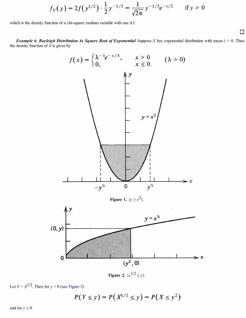
which is the density function of a chi-square random variable with one d.f.

Example 6. Rayleigh Distribution As Square Root of Exponential Suppose X has exponential distribution with mean λ > 0. Thenthe density function of X is given by

Figure 1. {y ≥ x2}.

Figure 2. {x1/2 ≤ y}.

Let Y = X1/2. Then for y > 0 (see Figure 2)

and for y ≤ 0

The density function of Y is obtained by differentiating P(Y ≤ y) with respect to y, and we have fY(y) = 2yf(y2) for y > 0. Hence

This is the density function of a Rayleigh distribution.

Example 7. Range of a Projectile. Let a projectile be fired with initial velocity u at an angle X where X has uniform distribution on(0, π/2). Let Y be the range of the projectile, that is, the distance between the point it was fired from and the point at which it returns toearth (Figure 3). We assume that the projectile is only under the effect of gravitational force. From calculus we know that Y = g–1u2sin2X where g is the gravitational constant assuming without loss of generality that the projectile was fired from the origin. Then thedensity function of X is given by

Figure 3. Range of the projectile.

Figure 4. {sin 2x ≤ g yu–2}.

Now for 0 < y < g–lu2 we have (see Figure 4)

Differentiating with respect to y we get the density function of Y as

In particular,

Indeed, if u2 > 10g, then

Example 8. Exponential Distribution As a Function of Uniform Distribution. Let X have uniform distribution on (0, 1). Then thedistribution of Y = ln(l/X) = – In X is given by

Hence, for y > 0 (Figure 5)

and

so that Y has an exponential distribution with mean one.

Example 9. X Is Continuous, Y = g(X) Is Discrete. Let X have density function given by

Let Y = g(X) where g(x) = [x] is the integral part of x, x > 0 (see Figure 6). Then for y ≥ 0, y integral,

and

Figure 5. {– ln x ≤ y}.

Figure 6. The function y = [x], x > 0.

Next we consider some examples when X is a random vector and Y = g(X) is a continuous typerandom variable.

Example 10. Sum of Jointly Distributed Random Variables. Let (X1, X2) have uniform distribution on the triangle {0 ≤ x1 ≤ x2 ≤1}. Then (X1, X2) has joint density function

Let Y = X1 + X2. Then for y < 0, P(Y ≤ y) = 0, and for y > 2, P(Y ≤ y) = 1. For 0 ≤ y ≤ 2, we have

There are two cases to consider according to whether 0 ≤ y ≤ 1 or l ≤ y ≤ 2 (Figures 7a and 7b). In the former case,

and in the latter case,

Figure 7. (a) {x1 + x2 ≤ y, 0 ≤ x1 ≤ x2 ≤ 1, 0 ≤ y ≤ 1}. (b) {x1 + x2 ≤ y, 0 ≤ x1 ≤ x2 ≤ 1 ≤ y ≤ 2}.

Hence the density function of Y is given by

Example 11. Difference of Independent and Uniformly Distributed Random Variables. Let (X1, X2) have a joint uniformdistribution on the unit square {(x1, x2): 0 < x1 < 1, 0 < x2 < 1}. Let Y = X1 – X2. Then

Clearly, P(Y ≤ y) = 0 if y ≤ –1, and P(Y ≤ y) = 1 if y ≥ 1. For |y| < 1 we need to consider two cases according to whether – 1 < y ≤ 0 or 0< y < 1 (see Figures 8a and 8b). For –1 < y ≤ 0, we have:

and for 0 < y < 1,

Figure 8. (a) {(x1, x2): –1 < x1 – x2 ≤ y ≤ 0). (b) {(x1, x2): 0 < x1 – x2 ≤ y < 1}.

Hence

In this particular case (and typically in cases where the distribution is uniform over a region) it is easy to compute P(Y ≤ y) by simplycomputing the volume of the solid with height f(x1, x2) = 1 and triangular cross section as shown in Figure 8a or 8b. Indeed, for –1 < y ≤0,

and for 0 < y < 1

We leave the reader to check that the density function of the random variable Y in Example 10 can also be obtained by a similarcomputation.

Example 12. Product of Two Uniformly Distributed Random Variables. Let X1, X2 be a random sample of size 2 from a uniformdistribution on (0, 1). Let Y = X1, X2. Then for 0 < y < 1 we have (Figure 9)

Figure 9. {(x1, x2): x1x2 ≤ y, 0 < x1, x2 < 1}

and

It follows that the density function of Y is given by

Example 13. Distribution of Proportion of Times a Machine Is in Operation. Let X1 be the time to failure of a machine and X2the repair time. Suppose X1 and X2 are independent exponentially distributed random variables with means λ1 and λ2, respectively. Thenthe proportion of time that the machine is in operation during any cycle is a random variable Y given by Y = X1/(X1 + X2). The distribution

function of Y is given by (Figure 10)

Figure 10.

Hence for 0 < y < 1,

and the density of Y is given by

In particular, if λ1 = λ2 then Y has uniform distribution on (0, 1).

The method of distribution functions can also be applied to compute the joint distribution of two ormore functions of a random Vector (X1, X2, …, Xk). The integration, however, becomes very complicated.We content ourselves here with the following example.

Example 14. Joint Distribution of X1 + X2 and X1 – X2 (Service Time at a Service Desk ). Let X1 be the time that a customertakes from getting on line at a service desk in a bank to completion of service, and let X2 be the time she waits in line before she reachesthe service desk. Then X1 ≥ X2 and X1 – X2 is the service time of the customer. Suppose the joint density of (X1, X2) is given by

Figure 11. {(x1, x2): x1 + x2 ≤ y1,x1 – x2 ≤ y2, 0 ≤ x2 ≤ x1 < ∞).

Let Y1 = X1 + X2 and Y2 = X1 – X2. Then the joint distribution of (Y1, Y2) is given by

where A = {(x1, x2): x1 + x2 ≤ y1, x1 – x2 ≤ y2, 0 ≤ x2 ≤ x1 < ∞}. Clearly, x1 + x2 ≥ x1 – x2 so that the set A is as shown in Figure 11.It follows that

Hence the joint density of Y1, Y2 is given by

The marginal densities of Y1, Y2 are easily obtained as

The Probability Integral Transformation and Its Applications

Let X be a random variable with distribution function F so that F(x) = P(X ≤ x) for x ∈ . What is thedistribution of the random variable Y = F(X)? Clearly, 0 ≤ Y ≤ 1, and for 0 < y < 1

If we can write F(X) ≤ y as X ≤ F–1(y), then

and Y will have uniform distribution on (0, 1). Unfortunately, F may not be strictly increasing or evencontinuous. If F is not continuous, then there is a jump at, say, X = a. That is, P(X = a) > 0 for some a. Inthat case, Y = F(X) takes the value F(a) with positive probability and Y itself is not of the continuous type.If, on the other hand, F is not strictly increasing, then F is “flat” on some interval, say (a, b) and F(x) = y0for all x ∈ (a, b). In that case, F does not have a unique inverse at y0 (Figure 12). If, however, F iscontinuous and strictly increasing, then F has a continuous and strictly increasing inverse F–1 over 0 < y <1 so that for 0 < y < 1

Figure 12

and

Consequently Y has uniform distribution on (0, 1).Suppose F is continuous. Then for 0 < y < 1 there exists a unique smallest x(y) such that F(x(y)) = y.

Formally:

Then

It follows that for 0 < y < 1

and Y has a uniform distribution on (0, 1). The transformation Y = F(X) is known as the probabilityintegral transformation.

Probability Integral TransformationIf X has a continuous distribution function F, then F(X) has uniform distribution on (0, 1).

In the case when X is discrete, F has jumps and it is clear from Figure 12 that for 0 < y < 1

In fact, if X takes values x1 < x2 < … with probabilities p1, p2,… then

Thus Y = F(X) is a discrete random variable which takes values p1, p1 + p2, p1 + p2 + p3,… withprobabilities p1, p2, p3,…. Moreover,

Probability integral transformation has important consequences in nonparametric statistics and incomputer simulation when one needs a random sample from a given distribution G.

PROPOSITION 1. Let G be any distribution function and X have uniform distribution on (0, 1). Then there exists a function hsuch that

Proof. If G is continuous, we choose h(X) = G–1(X). Then

If G has jumps of size pk at yk, k = 1, 2,… then we choose h as follows.

Then

and, in general,

Thus h(X) is a discrete random variable with distribution function G.

According to probability integral transformation, if X has density f and distribution function F, thenF(X) has uniform distribution on (0, 1). According to Proposition 1, if Y has density g and distributionfunction G, then Y = G–1(F(X)) transforms the density f into g. Thus any continuous type random variablecan be transformed into a random variable that has any desired continuous distribution by using theprobability integral transformation.

Example 15. Finding h Such That Y and h(X) Have the Same Distribution. Let X have density

Then

It follows that Z = F(X) = 1 – eX/λ has uniform distribution on (0, 1).Suppose Y has distribution function

Then U = G(Y) = 1 – 1/Y has uniform distribution on (0, 1). It also follows that Y = 1/(1 – U) = 1/e–X/λ = eX/λ has density g where g isthe density corresponding to G.

Also, –λ ln(1 – Z) has density f and 1/(1 – U) has density g in view of Proposition 1. Given a table of random numbers from uniformdistribution we can use it to obtain random samples from f and g.

Suppose, for example, that .41, .13, .90, .43, and .52 is a random sample of size 5 from the uniform distribution on (0,1). Then 1.06,0.28, 4.61, 1.12, and 1.47 is a random sample from the exponential density f with mean λ = 2 and 1.69, 1.15, 10.00, 1.75, and 2.08 is arandom sample from the density function g.

Problems for Section 8.2

1. Given X with probability function

Find the probability functions of:(i) Y = aX + b where a, b are nonnegative integers. (ii) Y = X2,

2. Suppose X has probability function

Let Y = g(X) = 1 if X is an even integer and Y = –1 if X is an odd integer. Find the probability function of Y.3. Suppose X has probability function

Find the probability function of Y = X2 + 4.4. Suppose X has probability function

Find the probability function Y = g(X) = X(mod3). That is, Y = 1 if X is of the form 3m + 1, Y = 2 if X is of the form 3m + 2, and Y = 0 if Xis of the form 3m + 3; m ≥ 0 is an integer.

5. Let Y be the output and X the input of an electrical device. The device is called a “full-wave” rectifier if Y = |X|. For a full-wave rectifier,find the density of the output if the density of the input is standard normal.

6. Let X be the (random) number of taxis that arrive at a taxi stand at O’Hare Airport (Chicago) during an interval of one hour. Let Y be thenumber of passengers who arrive at O’Hare and need taxi service during this time interval. Assume that X and Y are independent Poissonrandom variables; find the probability function of the excess of users over taxis, Y – X.

Figure 13. Position of the pointer after it comes to rest.

7. The temperature F, recorded in Fahrenheit, is related to temperature C measured in Centigrade by the relation C = 5(F – 32)/9. Supposethe temperature in Fahrenheit of a certain object has a normal distribution with mean μ and variance σ2. Find the distribution of C.

8. According to the kinetic theory of gases, the velocity V of a molecule of mass m in a gas at absolute temperature T has a Maxwelldistribution with density

where α = (2kT/m)1/2, k being the Boltzmann’s constant. Find the density function of the kinetic energy E = mV2/2 of a molecule.9. A pointer supported vertically one unit above the point of origin is spun and comes to rest at an angle Θ with the y-axis (Figure 13).

Suppose Θ has uniform distribution over [– π/2, π/2]. Let X be the distance (from the origin) of the point on the x-axis towards which thepointer is pointing. Find the distribution and density function of X

10. The tensile strength T of a wire is assumed to be proportional to the square of its diameter X. If X has uniform distribution over (a, b), 0 <a < b, find the distribution of T.

11. Let (X1, X2) have the joint probability function given in the following table

Find the probability functions of:

(i) X1 + X2. (ii) X1 – X2. (iii) |X1 – X2|. (iv) X1X2.

12. Let X1, X2 be independent random variables such that Xi has a negative binomial distribution with parameters ri and p, i = 1, 2. Find the

probability function of X1, + X2, [Hint: Use the identity

13. Let X1, X2 be independent random variables such that Xi has a binomial distribution with parameters ni, and p, i = 1, 2. Find the distributionof X1 + X2.

14. An urn contains four marbles marked 1 through 4. One marble is drawn at random and then all marbles with face values less than the onedrawn are removed from the urn. The first marble drawn is then replaced in the urn and a second marble is drawn. Let X1 be the numberon the first marble drawn, and X2 the number on the second marble drawn. Find the distributions of:

(i) X1 + X2. (ii) X2 – X115. A soft drink vending machine has a random amount X1 gallons in supply at the beginning of a given day. It dispenses an amount X2 gallons

during the day. Assuming that the machine is not resupplied during the day and that X1, X2 have joint density:

find the density of X1 – X2, the amount sold during the day.

16. Let X1, X2 have joint density

Find the density of X1X2.

17. Let R be the radius and T the thickness of hockey pucks manufactured by a certain manufacturer. Suppose R and T are independentlydistributed with uniform distributions over the intervals (5.0, 5.2) and (2, 2.05) centimeters respectively. What is the density function of thevolume of the puck?

18. Suppose X has a gamma density with parameters α > 0 and β = 1. Let Y be independent of X and have the same distribution as X. Find thedistributions of X + Y, X/Y, and X/(X + Y).

19. Let (X, Y) have joint density f which is uniform on the triangle bounded by 0 ≤ x ≤ 3, 0 ≤ y ≤ 1, and x ≥ 3y. Show that U = X – Y hasdensity

20. Suppose X has exponential density with mean λ and Y has density

Find a transformation y = h(x) such that if X has exponential density then h(X) has density g.21. Let (X, Y) have uniform density on the triangle 0 ≤ y ≤ x ≤ 1. Show that:

(i) W = X/Y has density fw(w) = 1/w2 for w ≥ 1 and fw(w) = 0 elsewhere.(ii) U = XY has density fU(m) = 2 + In u for 0 < u < 1 and fU(u) = 0 elsewhere.

22. Let X have uniform distribution on (0, 1). Show that Y = cos 3x has density function given by and 0 elsewhere.

23. Suppose X has density

and Y has density

Find the transformation Y = h(X).24. The following random sample was taken from the uniform distribution on (0,1):

.211 .023 .533 .144 .730 .641 .963.(i) Generate a random sample of size 7 from density function g of Problem 23.(ii) Generate a random sample from density function g of Problem 20.

8.3* THE METHOD OF TRANSFORMATIONS

In this section we restrict our attention to the case when X has a density function f and Y = g(X) itself is acontinuous type random variable. Frequently the function g is either (strictly) increasing or (strictly)decreasing. In such cases it is possible to compute the density of Y = g(X) directly without computing thedistribution function. Recall that for y ∈

We should like to be able to write P(g(X) ≤ y) as P(X ∈ A) where A is a subset of the real line (and is afunction of y and g). Whenever this is possible, we can obtain the density of Y by differentiating P(X ∈ A)with respect to y. This is certainly the case when g is (strictly) increasing or (strictly) decreasing over theset where f > 0. In either case, the mapping x → g(x) has a unique inverse g–1. That is, for every y there isone and only one x given by x = g–1(y) and, moreover, {g(X) ≤ y} = {X ≤ g–1(y)} or {X ≥ g–1(y)}according to whether g is increasing or decreasing. See Figures 1a and 1b.

Figure 1. (a) g increasing, (b) g decreasing.

Suppose g is increasing. In that case:

where F is the distribution function of X. Differentiating with respect to y we get the density of Y as

where x = g–1(y). In the case when g is decreasing, on the other hand,

since X is a continuous type random variable. Hence

Since, however, g is decreasing, so is g–1 and dx/dy is negative. It follows that in either case

The Density Function of Y = g(X) When g Is Increasing or Decreasing

It should be clear that this method can be extended to the case when the real line can be partitionedinto intervals An such that g is either strictly increasing or decreasing on each An. We can define

and write . Then gn has a unique inverse in An. If we write

then we can consider each gn separately and sum over all n. We have

A few examples of this type will also be given in this section.

Example 1. A Linear Function of Uniformly Distributed Random Variable. Let X have uniform distribution on (0, 1) and let y =g(x) = 2x + 4. Since Y = 2X + 4 simply changes the origin and scale, we expect the distribution of Y to be uniform. Note that g isincreasing on (0, 1) and the inverse function is obtained by solving y = 2x + 4 for x. Indeed, so that

so that

It follows that

We note that Y has uniform distribution on (4, 6).

Example 2. Square of Exponential Random Variable. Let X have exponential density

The function y = g(x) = x2 is strictly decreasing on the set {f(x) > 0} = (–∞, 0) so that the inverse function is x = g–1(y) = –yl/2. Thus

and

for y > 0. For y < 0, however,

Example 3. Square of Normal (0,1). We consider Example 8.2.5 again, where X has a standard normal distribution and g(X) = X2.The function g is decreasing over (–∞, 0) and increasing over (0, ∞) and we can no longer apply (3) or (6) directly. The function y = x2,for y > 0, has a unique inverse x1 = – on (– ∞, 0) and a unique inverse x2 = on (0, ∞) (Figure 2). We apply (7) to get

for y > 0 and fY(y) = 0 for y ≤ 0.

Example 4. Distribution of Y = sin X for X Uniform. Let X have uniform distribution on the circumference of unit circle withdensity function

Figure 2. y = x2

Let Y = g(X) = sin X. Clearly –1 < Y < 1 (with probability one). We note that g′(x) = cos x > 0 for 0 < x < π/2 or 3π/2 < x < 2π and g′(x)< 0 for x ∈ (π/2, 3π/2), so that g is increasing over (0, μ/2) ∪ (3π/2, 2π) and decreasing over (π/2, 3π/2). (See Figure 3.) We need toseparate the two cases according to whether 0 < y < 1 (equivalently, 0 < x < π) or – 1 < y < 0 (equivalently, π < x < 2π). In the formercase there are two inverses x1 = sin–1y, x2 = π – sin–1y; in the latter case the inverses are

Hence for 0 < y < 1:

and for – 1 < y < 0:

Figure 3. y = sin x on (0, 2π).

Clearly, fY(y) = 0 for |y| > 1. Hence

The method of transformations can also be applied in the multivariate case. Rather than develop ageneral method, we will content ourselves with some examples to illustrate how the above method for theunivariate case can be used in the multivariate case as well. In the bivariate case, the trick is to hold oneof the variables, say X2, fixed and then find the joint distribution of Y = g(X1, X2) and X1 (or X2 if X1 isheld fixed). The distribution of Y is then obtained by computing the marginal distribution of Y from thejoint distribution of (Y, X1).

Example 5. Sum of Poisson Random Variables. We consider Example 8.2.4 again, where we computed the distribution of Y =g(X1, X2) = X1 + X2 in the case when X1, X2 are independent random variables with Poisson distributions. Assume λ1 = λ2. Then

and the joint probability function of Y and X1 is given by

Summing over x1 = 0, 1, 2, … we get

Example 6. Distribution of X1/ (X1 + X2) for Independent Exponentially Distributed Random Variables. We return to Example8.2.13, where we computed the distribution of Y = X1/(X1 + X2) where X1, X2 were independent exponentially distributed randomvariables with means λ1 and λ2 respectively. For convenience, we consider only the λ1 = λ2 = λ case. Then X1 and X2 have joint densityfunction

Let y = x1/(x1 + x2) and suppose we hold x1 constant. Then y decreases as x2 increases and we can apply (6) to find the joint density of

Y and X1 Now y = x1/(x1 + x2) implies x2 = x1(1 – y)/y so that ∂x2/∂y = –x1/y2. It follows from (6) that X1 and Y have joint density

for x1 > 0, 0 < y < 1, and u(x1, y) = 0 elsewhere. Hence the marginal of Y is given by

and fY(y) = 0 elsewhere.

Example 7. Distribution of X1 + X2 + X3. Let X1, X2, X3 have joint density

Let y = g(x1, x2, x3) = x1 + x2 + x3. We first find the density of Y, X2, X3. Note that g increases as x1 increases (for fixed x2, x3), sothat from (6)

Now x1 = y – x2 – x3 and ∂x1/∂y = 1 and it follows that

for x2, x3 > 0 and y > x2 + x3, and u(y, x2, x3) = 0 otherwise. Finally, the marginal of Y is given by

and fY(y) = 0 elsewhere.

In Section 8.6 we will consider yet another method of obtaining distribution of g(X1, X2, …, Xn) giventhat of (X1, X2, …, Xn). This method is frequently useful when X1, X2, …, Xn are independently distributedand .

Problems for Section 8.3

1. Let X have density function f and Y = aX + b where a(≠ 0) and b are constants. Find the density of Y.

2. Let X have density f(x) = 2x for 0 < x < 1 and f(x) = 0 otherwise. Find the density function of Y = e–X.3. Let X be uniformly distributed over (0, 1). Find the density function of:

(i) Y = X2. (ii) Y = 1/(X + 1). (iii) Y = 1 /X.(iv) Y = X1/β, β ≠ 0. (v) Y = –λ ln X, λ > 0. (vi) Y = X/(1 + X).

4. A straight line is drawn at random through the point (0, 1) in the sense that the angle Θ between the line and y = 1 is uniformly distributedover the interval (0, π). Let X be the length of the perpendicular from the origin to this line (Figure 4). What is the probability densityfunction of X?

5. Let X have standard normal distribution. Find the density of Y = {|X|}1/2.6. Let X have density f. Find the density of

(i) Y = Xn, when n is an odd positive integer > 1.(ii) Y = Xn, when n is an even positive integer.(iii) Y = exp{aX + b }, a ≠ 0.

7. Let X be normal with mean μ and variance σ2. Show that Y = eX has lognormal density function

8. Let X be a positive random variable having density function f. Find the density functions of:

(i) Y = (X)–1. (ii) Y = 1/(X + 1).(iii) Y = X/(X + 1). (iv) Y = e–X.

9. Let X have density f(x) = (1/λ)e–x/λ, x > 0, and f(x) = 0 otherwise. Find the density functions of:(i) Y = – X. (ii) Y = X/(1 + X).

10. Let X have Cauchy density f(x) = [π(1 + x2)]–1, x ∈ . Show that Y = 1/X has the same density as X.

11. Suppose X has density f(x) = (1 + x)–2 for x > 0 and f(x) = 0 elsewhere. Show that Y = 1/X also has density f.

Figure 4

12. Suppose X has density function

Show that Y = e–X has density function

13. Let X have density function

Show that Y = X2 has density

14. Let X1, X2 be the lengths of life of two different types of components operating in a system. Then Y = X1/X2 is a measure of the relativeefficiency of component 1 with respect to component 2. Suppose (X1, X2) has joint density given by

Find the density of Y.15. Let X1, X2 be independent random variables with common uniform density

Show by transformation technique that the density of Y = X1 + X2 is given by

16*. Let X1, X2, X3 have joint density given by

Find the density of Y = X1 + X2 + X3.

17. Let X1, X2 be independent random variables each having geometric distribution with parameter p, 0 < p < 1. Show that Y = X1 + X2 has anegative binomial distribution.

18. Let X be a uniformly distributed random variable on (0, 1) and let Y be independent of X and have density fY(y) = 1 – |y| for |y| < 1 andfY(y) = 0 otherwise. The random variable X + Y is observed. Find its density.

19. Let X and Y be independent random variables having a common exponential density with mean one. Find the density of .

20. A missile is fired and lands at ( X, Y) where X is the latitudinal distance in meters and Y the longitudinal distance in meters from the target.If X and Y are independent with common normal distribution having mean zero and variance σ2, show that has a

Rayleigh density given by fZ(z) = (z/σ2)exp(–z2/2σ2), z > 0, and = 0 elsewhere.

21*. If X and Y are independent with common uniform distribution on (0,1), find the joint density of X + Y and X – Y.22. Suppose a simple electrical circuit contains a constant voltage source and a resistor. Let E be the voltage assumed to be constant. Suppose

the resistor is chosen randomly from a stack where the resistance R has density function f(r) = (r/λ2)exp{– r/λ} for r > 0 and f(r) = 0 forr ≤ 0. According to Ohm’s law the current I passing through the circuit is determined by I = E/R.(i) Find the density function of I.(ii) Find the density function of W, the power dissipated in the resistor, where W = I2R = E2/R = EI.

8.4 DISTRIBUTIONS OF SUM, PRODUCT, AND QUOTIENT OF TWORANDOM VARIABLES

Let (X1, X2) have a joint distribution given by its joint probability or density function. In manyapplications we shall be interested in the distribution of random variables X1 + X2, X1X2, and X1/X2. Forexample, if X1, X2 are two sides of a rectangle, then the area is given by X1X2, the perimeter by 2(X1 + X2)and, given the area and one of the sides X1 the remaining side is given by area/X1. If proportion X2 of acompound is sampled and X1 is the proportion of chemical A in the sample, then the proportion ofchemical A in the compound is X1X2, and so on.

In this section we compute the distributions of X1 + X2, X1X2, and X1/X2 in terms of the jointdistribution of (X1, X2) by using methods of Section 8.2. Methods of Section 8.3 can also be applied toyield the same results. Some special cases have already been considered in several examples in Sections8.2 and 8.3. See also Problem 5.5.13.

Let us first dispense with the discrete case. Let

be the joint probability function of (X1, X2). Then

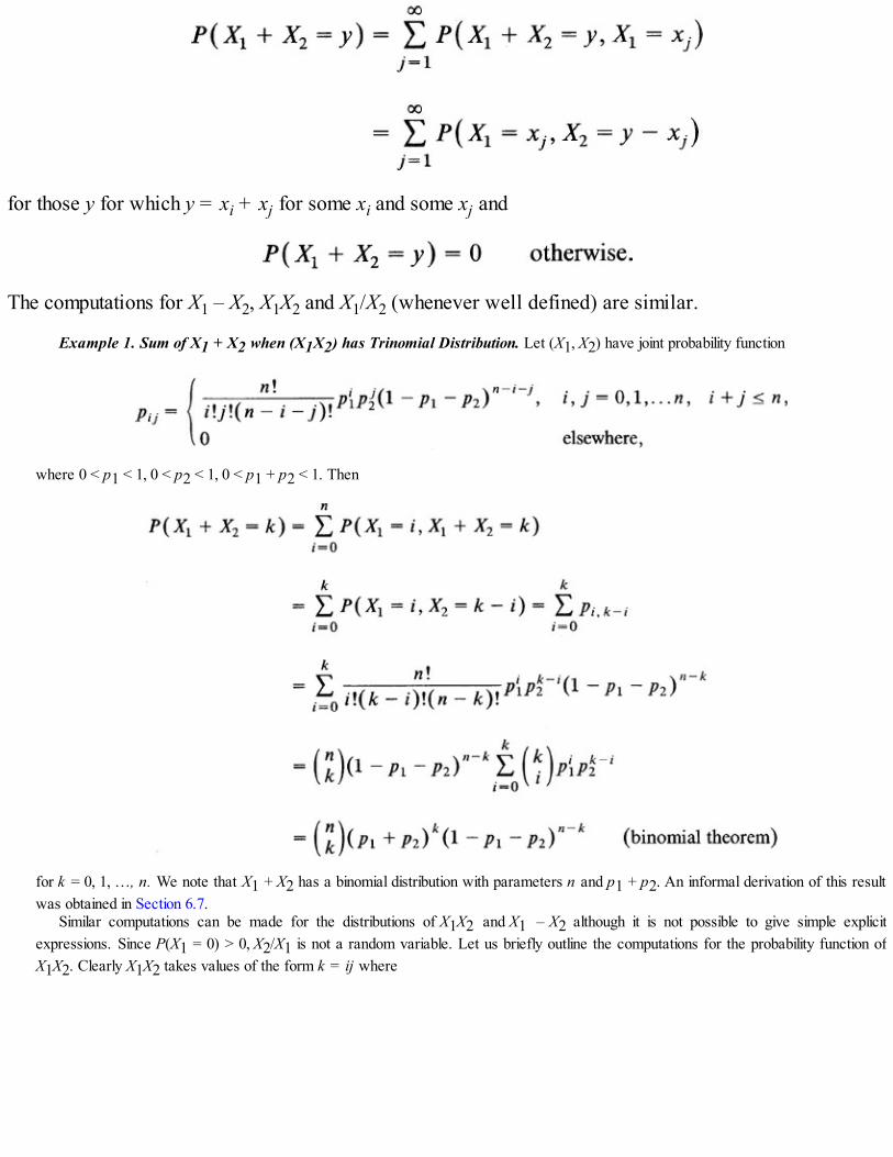
for those y for which y = xi + xj for some xi and some xj and

The computations for X1 – X2, X1X2 and X1/X2 (whenever well defined) are similar.

Example 1. Sum of X1 + X2 when (X1X2) has Trinomial Distribution. Let (X1, X2) have joint probability function

where 0 < p1 < 1, 0 < p2 < 1, 0 < p1 + p2 < 1. Then

for k = 0, 1, …, n. We note that X1 + X2 has a binomial distribution with parameters n and p1 + p2. An informal derivation of this resultwas obtained in Section 6.7.

Similar computations can be made for the distributions of X1X2 and X1 – X2 although it is not possible to give simple explicitexpressions. Since P(X1 = 0) > 0, X2/X1 is not a random variable. Let us briefly outline the computations for the probability function ofX1X2. Clearly X1X2 takes values of the form k = ij where

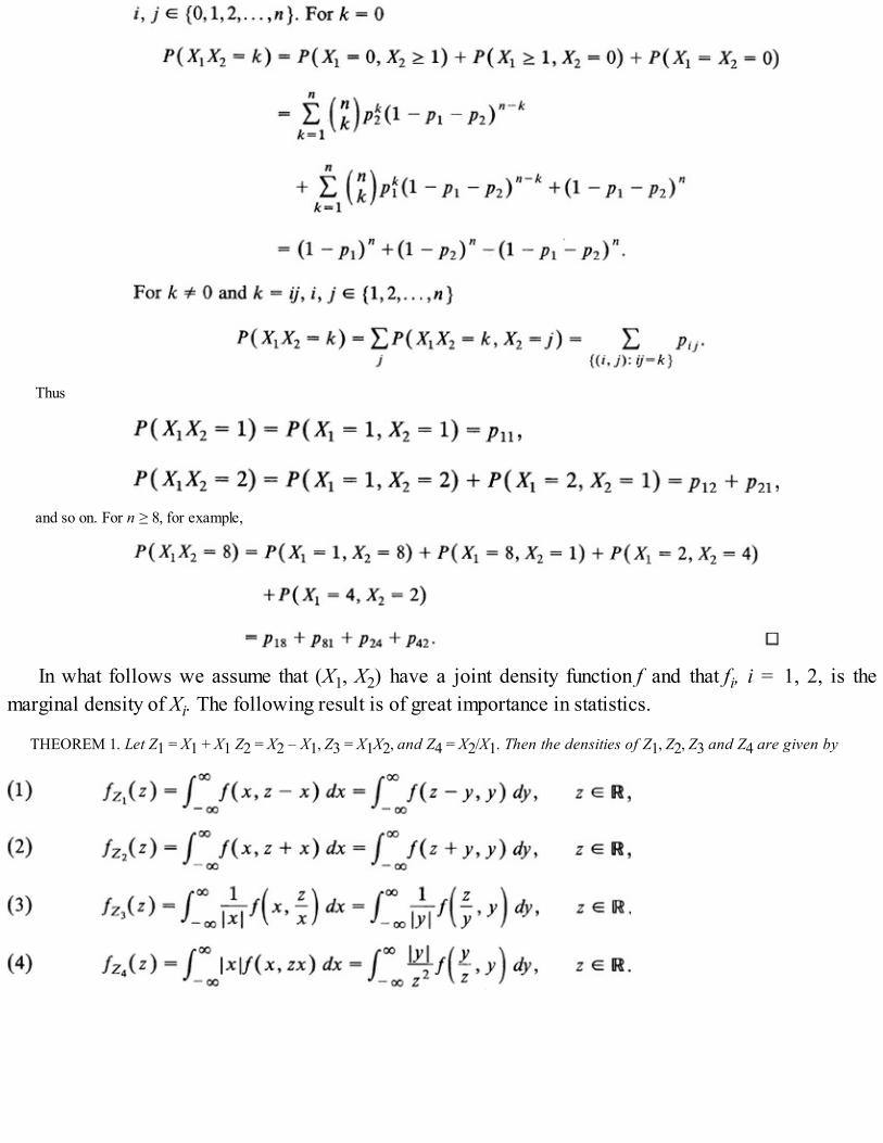
Thus

and so on. For n ≥ 8, for example,

In what follows we assume that (X1, X2) have a joint density function f and that fi, i = 1, 2, is themarginal density of Xi. The following result is of great importance in statistics.

THEOREM 1. Let Z1 = X1 + X1 Z2 = X2 – X1, Z3 = X1X2, and Z4 = X2/X1. Then the densities of Z1, Z2, Z3 and Z4 are given by

Figure 1. {(x, y): x + y ≤ z}.

Proof From Figure 1

so that on differentiating with respect to z we have

Interchanging x and y we get the second part of (1).As for Z2, we have from Figure 2:

and on differentiation with respect to z we get:

Interchanging the role of x and y we get the second part in (2).

Figure 2. {(x, y): x – y ≤ z}.

Next we consider Z3. In this case we note that

Consequently (see Figures 3a and 3b) we have

It follows that

Interchanging the role of x and y we get the second equality in (3).Finally we consider Z4. In this case,

Figure 3. (a) {xy ≤ z} for z > 0. (b) {xy ≤ z} for z < 0.

Note, however, that if X < 0, then

so that

In view of Figures 4a and 4b, we have

Differentiating with respect to z we get

and interchanging the roles of x and y we get the second part of (4).

Figure 4. (a) {y/x ≤ z} for z > 0. (b) {y/x ≤ z} for z < 0.

The case of most interest in applications is the case when X1 and X2 are independent. In this case wecan rewrite Theorem 1 in terms of the marginal densities of X1 and X2 as follows.

THEOREM 2. Let X1, X2 be independent random variables of the continuous type with densities f1and f2 respectively. Then, for z ∈ :

The two right sides of (5) suggest a simple method of obtaining densities. Given two (one-dimensional) densities f and g, the function h defined by

itself is a one-dimensional density function which is known as the convolution of f and g. In view ofTheorem 2, the density of the sum of two independent continuous type random variables is the convolutionof their individual densities. However, it does not follow that if h is a convolution density obtainedfrom densities of X1 and X2 then X1 and X2 are independent. (See Example 2 below.)

A similar definition is given in the discrete case. The probability function defined by

is known as the convolution of probability functions P(X1 = x) and P(X2 = y). Similar remarks apply tothe discrete case.

Example 2. Random Variable X1 + X2 with Convolution Density of Non-independent X1, X2. Let (X1, X2) have joint density

Then f1(x1) = f2(x1) = 1/2 for |x1| < 1 and 0 elsewhere. It follows that X1 and X2 are dependent. Let Z = X1 + X2. We show that thedensity of Z is the convolution of f1 and f2. In fact, from (1):

Now f(x1, z – x1) > 0 over |x1| < 1 and |z – x1| < 1, that is, over |x1| < 1 and x1 – 1 < z < x1 + 1 (Figure 5). Rewriting the domain ofpositivity of f(x1, z – x1) as –1 < x1 and Z – 1 < x1 < z + 1, and noting that for z < 0, z – 1 < 1 and z + 1 < 1, and for z > 0, z – 1 > –1 andz + 1 > 1, we have

Figure 5. {|x1| < 1, |z – x1| < 1).

Finally, the convolution of f1 and f2 is given by

It follows that even though the density of X1 + X2 is the convolution of the densities of X1 and X2, the random variables X1 and X2 are notindependent.

Example 3*. An Application to Beta Functions. Let α1, α2 > 0. As an application of (5) we show that

which was proved in Proposition 7.3.4 (iii) by a somewhat complicated method. Let X1, X2 be independent random variables such that Xihas a gamma density with parameters α = αi and β = 1, i = 1, 2. Let Z = X1 + X2. Then for z ≤ 0, fZ(z) = 0 and for z > 0 in view of (5)

Since fZ is a density function we must have

It follows that

and, moreover, that Z itself has a gamma distribution with parameters α = α1 + α2, β = 1.

Example 4. Lifetime of a System with Two Components . Let X1, X2 represent the lifetimes of two components, an original and itsreplacement. Then Y = X1 + X2 represents the lifetime of the system consisting of this pair. It is of interest to find the survival functionP(X1 + X2 > a) for a > 0. Suppose X1 and X2 are independent exponential random variables with common mean λ > 0. Then the jointdensity of (X1, X2) is given by

The density of Y = X1 + X2 is given by

for y > 0 and

Thus Y has a gamma distribution with parameters α = 2 and β = λ. Moreover, for a > 0

Suppose next we wish to find the probability that the replacement outlasts the original component. Since X2 – X1 is a symmetricrandom variable (see Problem 3.8.16),

Let us compute the density of Z = X2 – X1 In view of (6), we have for z > 0

and for z < 0

It follows that

which is known as a double exponential or Laplace density function.

In Examples 5 and 6 we consider some important distributions in Statistics which arise as ratios ofcertain independent random variables.

Example 5. Student’s t-distribution. Let X have a standard normal distribution and let Y be independent of X and have a chi-squaredistribution with n degrees of freedom. Then the random variable is said to have Student’s t-distribution with n

degrees of freedom. Let us compute the density function of T. We note that Y has density

since Y is a gamma variable with α = n/2 and β = 2 (see Section 7.4). The density of , therefore, is given by

and

Since X and Y are independent, so are X and U, and from Theorem 2 [equation (8)] the density of T is given by

Setting z = u2(n + t2)/2 so that u = (2z/(n + t2))1/2 and dz = (n + t2)u du, we have

Example 6. The F-Distribution. Let X and Y be independent random variables such that X has a chi-square distribution with m d.f.and Y has a chi-square distribution with n d.f. Then the random variable

is said to have an F-distribution with (m, n) d.f. We compute the density of F. We note that the density of X/m is given by

and that of Y/n by

In view of (8), the density of F is given by

and

Problems for Section 8.4

1. The random variables X1 and X2 measure the errors in two measurements. Assume that X1, X2 are independent and each is uniformlydistributed over (0,1). Find the density functions of(i) Y1 = X1 – X2. (ii) Y2 = X1X2. (iii) Y3 = X1/X2.

2. Let X1, X2 measure the lifetimes of two components operating independently. Suppose each has density (in units of 100 hours)

if measures the quality of the system, show that Y has density function

3. Let X1 and X2 be independent standard normal random variables. Show that Y = X1/X2 is a Cauchy random variable with density fY(y) =

[π(1 + y2)]–1, y ∈ .

4. Let X1 and X2 be independent with common density

Find the density of X1X2.

5. Suppose X1, X2 are independent random variables with common density

Find the density of X1/X2.

6. Find the density of X1/X2 if X1 and X2 have joint density

7. Let X1, X2 be independent random variables with common probability function P(Xi = x) = 1/N, x = 1, 2, …, N; i = 1, 2. Find theprobability functions of X1 + X2 and X1 – X2.

8. Let (X1, X2) have joint probability function given by

Find the probability function of X1 + X2.

9*. Suppose X1 is uniform on (–2, 2) and X2 has density f2(x2) = 1 – |x2| for |x2| < 1 and f2(x2) = 0 elsewhere. Show that their convolutiondensity is given by

10. Suppose (X, Y) has joint density given by

Show that(i) X + Y has density f1(z) = z2, 0 < z < 1, = z(2 – z), 1 < z < 2, and 0 elsewhere.(ii) XY has density f2(z) = 2(1 – z), 0 < z < 1, and 0 elsewhere.(iii) Y/X has density f3(z) = (1 + z)/3, 0 < z < 1, = (1 + z)/3z , z > 1, and 0 elsewhere.(iv) Y – X has density f4(z) = 1 – |z|, |z| < 1, and 0 elsewhere.

11*. Suppose (X, Y) has joint density

Show that Z = X + Y has density

12. Suppose (X, Y) has joint density

Find the density of X + Y.13*. Let F be any distribution function and ε > 0. Show that

and

define distribution functions. (Hint: Use convolution result.)14*. Let X, Y, Z be independent random variables with common uniform distribution on [0, 1]. Show that X + Y + Z has density

(Hint: Convolute X + Y with Z and use the result of Problem 8.3.15.)15. For the bivariate distribution given by

show that the probability function of X + Y is the convolution of probability functions of X and Y.16*. Let X, Y have a bivariate normal distribution with μ1 = μ2 = 0, σ1 = σ2 = 1, and correlation coefficient ρ. Show that X/Y has density

17. Let (X, Y) have joint density

Find the convolution density of X and Y Is it the same as the density of X + Y?18*. Let X1, X2, X3 be independent random variables each having exponential density with mean λ. Find the density of X1 + X2 + X3.

19. If Fhas an F distribution with (m, n) d.f. show that 1/Fhas an F distribution with (n, m) d.f.20. Suppose X has an Fdistribution with (m, n) d.f. Show that Y = mX/(mX + n) has a beta distribution.

8.5 ORDER STATISTICS

In many applications the relative magnitude of the observations is of great interest. If a manufacturing firmwants to estimate the average time to failure of its bulbs based on a sample of size n, the sample mean can be used as an estimate of μ. In Section 5.5 we saw that is an unbiased estimate of μ. In fact, isthe best estimate of μ in many models when the object is to minimize the variance of the estimate (Section10.3). In order to compute , however, the manufacturer needs to wait until the last bulb has fused, and itmay be a very long wait indeed. On the other hand, an estimate can be used based on the least time tofailure. This estimate may not be as good as in that its variance may be larger than that of , but it canbe computed as soon as the first bulb fuses. (See Example 2.) In this section we consider distributions ofcertain statistics obtained by ordering the observations.

Let X1, X2, …, Xn be a random sample from a distribution function F with density function f. Let usorder the observations according to increasing order of their magnitude and write X(1), X(2), …, X(n) forthe ordered random variables. Then

and Xj, j = 1, 2, …, n are called order statistics. Note that equality holds with probability zero (why?).Thus

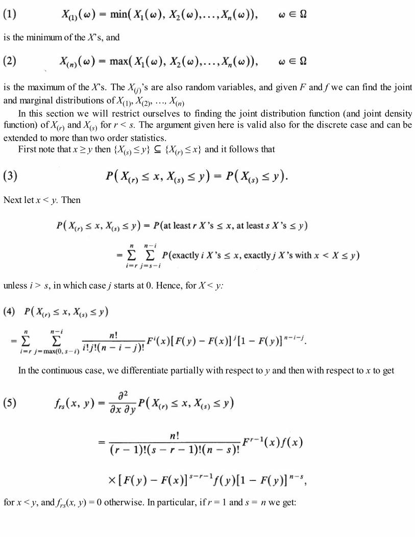
is the minimum of the X’s, and

is the maximum of the X’s. The X(j)’s are also random variables, and given F and f we can find the jointand marginal distributions of X(1), X(2), …, X(n)

In this section we will restrict ourselves to finding the joint distribution function (and joint densityfunction) of X(r) and X(s) for r < s. The argument given here is valid also for the discrete case and can beextended to more than two order statistics.

First note that x ≥ y then {X(s) ≤ y} ⊆ {X(r) ≤ x} and it follows that

Next let x < y. Then

unless i > s, in which case j starts at 0. Hence, for X < y:

In the continuous case, we differentiate partially with respect to y and then with respect to x to get

for x < y, and frs(x, y) = 0 otherwise. In particular, if r = 1 and s = n we get:

The marginal density of X(r), 1 ≤ r ≤ n can be obtained by integrating frs(x, y) with respect to y or directlyby computing the distribution function of X(r). In fact,

In the continuous case, we differentiate† (7) with respect to x to obtain

so that for x ∈

In particular,

and

In general, it can be shown (in the continuous case) that

Distribution of Order Statistics in Sampling from a Density Function f with Distribution Function F

Remark 1. Since X(1) ≤ X(2) ≤ … ≤ X(n) we cannot expect the X(i)’s to be independent. Indeed they aredependent unless the common distribution of the X’s is degenerate at some constant c. We leave the readerto supply a proof in Problem 27.

Example 1. Distribution of Maximum in Binomial Sampling. Let X1, X2, …, Xk be a sample from a binomial population withparameters n and p. Let X(r), 1 ≤ r ≤ k be the rth order statistic. Then, from (7):

for l = 0, 1, 2, …, n where Hence, for l ≥ 1,

and

Example 2. Length of Life of a System with n Components Operating in Series or Parallel Consider a system of n identical

batteries operating independently in a system. Suppose the length of life has common density function

We first consider the case when the batteries operate in series (Figure 1) so that the system fails at the first battery failure.Since the system fails at the first failure, the length of life Y of the system is given by

In view of (8) with r = 1, the density function of Y is given by

Since F(y) = 1 – e–y/λ for y > 0 we have

It follows that Y itself has an exponential distribution with mean λ/n.If the object is to estimate λ, then

so that nY is an unbiased estimate of λ. Note that is also unbiased. Moreover,

Figure 1. n Batteries in series.

Also,

so that

Yet nY may be preferred over as an estimate of λ.On the other hand, if the batteries operate in parallel (Figure 2), the system fails if all the n batteries fail. In this case, the length of life

of the system equals

with density function

Example 3. The Distribution of Range of a Random Sample. Let X1, X2, …, Xn be a random sample from a distribution functionF with density function f. A somewhat crude measure of the variation in the sample is the range R defined by R = X(n) – X(1). Wecompute the distribution of R by using (6) and (8.4.2). In view of (8.4.2), we have for r > 0

Figure 2. n Batteries in parallel.

and for r ≤ 0,

If in particular X1, X2, …, Xn are n points chosen at random and independently from [0, 1], then

In this case f(x) f(x + r) > 0 if and only if 0 ≤ x < x + r ≤ l, and it follows (Figure 3) from (10) that for 0 < r < 1

and

We note that R has a beta density with α = n – 1 and β = 2. For n = 2, the density of the range is given by

which is not the density of X1 – X2 as computed in Example 8.2.11. The range in this case is in fact

Figure 3. {(x, r): f(x)f(x + r) > 0}.

We leave the reader to check that the density of |X1 – X2| as computed from Example 8.2.11 coincides with the one obtained above.

Example 4. Estimating θ for Uniform Distribution on (0, θ). Let X1, X2, …, Xn, n ≥ 2, be a sample from a uniform distribution on(0, θ). We consider the performance of several estimates of θ some based on order statistics. First we note that

is unbiased for θ with variance σ21 = 4 θ2/12n = θ2/3n. Next we note that Mn = max(X1, …, Xn) has density function

so that

and

It follows that

is unbiased for θ with variance

Finally, we consider the range R = max{X1, …, Xn) – min{X1, …, Xn} and note that R has density

Hence

and it follows that

is also unbiased for θ. Moreover,

Hence

It is easily checked that σ32 > σ2

2 for n ≥ 2 so that 2 is a better estimate of θ than 3 if the criteria used is to choose an estimate

with a smaller variance. Moreover, σ21 > σ2

2 so that 2 is the best of the three estimates considered here in terms of minimum variance.This is essentially a continuous version of the taxi problem considered in Example 6.2.1.

8.5.1 Estimation of Quantiles of a Distribution

The quantiles provide important information about the shape of a distribution. Often one knows littleabout the distribution being sampled. Knowledge of a few quantiles provides important information abouthow the distribution assigns probabilities.

We recall (Section 3.7) that a quantile of order p of a random variable with distribution function F isa number ζp(F) that satisfies

so that ζp(F) is a solution of

If P(X = x) = 0, as is the case, in particular, if Xis of the continuous type, then ζp is a solution of theequation

If F is strictly increasing, ζp is uniquely determined by (12). We recall also that for p = 1/2 we call ζp(F)a median of F. Quantiles have the advantage that they can be estimated from the sample without theknowledge of the form of F, that is, nonparametrically. Moreover these estimates are easy to compute.

In what follows we will assume, unless otherwise specified, that F is continuous and strictlyincreasing so that (12) has a unique solution. Let X1, X2, …, Xn be a random sample from F. How do weestimate ζp(F), given p, 0 < p < 1? An intuitive answer is to use the sample quantile of order p to estimateζp. (This is the so-called substitution principle, which is discussed in detail in Section 10.4.) Since F iscontinuous, we can arrange the observations in an increasing order of magnitude as

Recall (Remark 3.8.5) that when n = 2m + 1, there is a unique middle value X(m + 1) which is the samplemedian. If n = 2m, then X(m) and X(m+1) are two middle values and any number between X(m) and X(m+1)may be taken as a median. We adopted the convention that in this case we will take (X(m) + X(m+1))/2 asthe sample median. Similar problems arise when we try to define a sample quantile of order p, 0 < p < 1.If n is large, however, the range of possible values of the sample quantile of order p will be small, and itdoes not really matter which possible value is taken to define the sample quantile. For this reason, wedefine the sample quantile of order p by

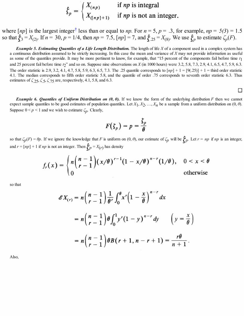
where [np] is the largest integer† less than or equal to np. For n = 5, p = .3, for example, np = 5(3) = 1.5so that 3 = X(2). If n = 30, p = 1/4, then np = 7.5, [np] = 7, and .25 = X(8). We use p to estimate ζp(F).

Example 5. Estimating Quantiles of a Life Length Distribution. The length of life X of a component used in a complex system hasa continuous distribution assumed to be strictly increasing. In this case the mean and variance of X may not provide information as usefulas some of the quantiles provide. It may be more pertinent to know, for example, that “15 percent of the components fail before time t1and 25 percent fail before time t2” and so on. Suppose nine observations on X (in 1000 hours) were 3.2, 5.8, 7.3, 2.9, 4.1, 6.5, 4.7, 5.9, 6.3.The order statistic is 2.9, 3.2, 4.1, 4.7, 5.8, 5.9, 6.3, 6.5, 7.3. The .25 quantile corresponds to [np] + 1 = [9(.25)] + 1 = third order statistic4.1. The median corresponds to fifth order statistic 5.8, and the quantile of order .75 corresponds to seventh order statistic 6.3. Thusestimates of ζ.25, ζ.5, ζ.75 are, respectively, 4.1, 5.8, and 6.3.

Example 6. Quantiles of Uniform Distribution on (0, θ). If we know the form of the underlying distribution F then we cannotexpect sample quantiles to be good estimates of population quantiles. Let X1, X2, …, Xn be a sample from a uniform distribution on (0, θ).Suppose 0 < p < 1 and we wish to estimate ζp. Clearly,

so that ζp(F) = θp. If we ignore the knowledge that F is uniform on (0, θ), our estimate of ζp will be p. Let r = np if np is an integer,

and r = [np] + 1 if np is not an integer. Then p = X(r) has density

so that

Also,

Thus

On the other hand, the knowledge of F allows us to choose the estimate

from Example 4. It is clear that so that 1 is unbiased and

again from Example 4. It should not be surprising if MSE( 1) ≤ MSE(X(r)) since 1 uses the knowledge that F is uniform on (0, θ)whereas X(r) is the estimate of ζp no matter what F is.

We leave the reader to check that MSE( 1) < MSE(X(r)).

Some large sample properties of order statistics as estimates of quantiles will be taken up in Section9.8. We now consider the problem of constructing confidence intervals for quantiles. This problem has aneasy solution, as we show. Let X1, X2, …, Xn be a random sample from a distribution function F whichmay be discrete or continuous. Let X(1) ≤ X(2) ≤ … ≤ X(n) be the order statistic. Suppose we want aconfidence interval for ζp(F) = ζp for 0 < p < 1 (p known). Recall that ζp is a solution of

Let Y be the number of Xi’s that are less than or equal to ζp. Then Y has a binomial distribution withparameters n and P(Xi ≤ ζp) = F(ζp). Hence

Similarly,

In view of (13) and (14), we have for r < s

since F(ζp–) ≤ p ≤ F(ζp) with equality if F is continuous. [We have used inequality (7.5.6′).] Suppose wewant a confidence interval for ζp at level at least 1 – α. Then we choose r and s such that

so that

This is done easily with the help of a binomial distribution table such as Table A3. In practice we chooser and s to minimize s – r subject to (16).

We emphasize that since the binomial distribution function [used on the left side of (16)] is discretegiven α, a 1 – α level confidence interval [X(r), X(s)] for ζp may or may not exist. If F is continuous, thenthere is equality in (15). Nevertheless, not every level 1 – α is attainable. (See Problems 18 and 28.)

Example 7. Confidence Interval for “Half-Lifetime” or “Median Lifetime” for Example 5. Let us compute a 95 percentconfidence interval for the median lifetime ζ.5 of the component. Since n = 9, p = .5, and α = .05, we need to choose r and s such that s –r is the least from

From Table A3 we see that s = 8 and r = 2 gives a confidence interval of level .9806 – .0196 = .9610. Hence a 95 percent confidenceinterval is [X(2), X(8)] = [3.2, 6.5].

Often the problem is to find the sample size n such that [X(r), X(s)] is a confidence interval for ζp at level ≥ 1 – α. Given r, s, p and αthis is done by solving (16) for n. In particular, suppose we want the sample size n such that [X(1), X(n)] is a 99 percent confidenceinterval for the median. Then we need to solve

for n. It follows from Table A3 that n = 8.

8.5.2 Testing Hypothesis Concerning Quantiles

The problem of testing H0: ζp(F) = ζ0 against one-sided or two-sided alternatives when F is continuous isalso simple. For example, if the alternative is H1: ζp(F) > ζ0, then we can use some order statistic X(r) totest H0. Under H0,

If the level of significance α is specified, then we choose the largest r such that

in view of (13). We reject H0 if the observed value of X(r) is greater than ζ0.A simpler procedure is to consider Yi = Xi – ζ0, i = 1, 2, …, n. Then count the number S of negative

signs among the Y’s. A small value of S tends to support H1 so that we reject H0 if S is small. This isprecisely the sign test of Section 6.3.2. In fact, under H0, P(Yi < 0) = P(Xi < ζ0) = p and S has a binomialdistribution with parameters n and p. We reject H0 if S ≤ c, say, where c is chosen from

Alternatively, we compute the P-value

where s0 is the observed number of negative Y’s. The magnitude of the P-value determines whether or notwe reject H0 at level α.

Note that

X(r) > ζ0if and only if there are at least n – r + 1 plus signs in the Y ‘s or equivalently atmost r – 1 negative signs among the Y’s.

Hence the test with critical region X(r) > ζ0 is equivalent to the test with critical region S ≤ r – 1. Theprocedure is similar for testing ζp(F) = ζ0 against ζp(F) < ζ0 or ζp(F) ≠ ζ0. We refer to Section 6.3.

We conclude our discussion with the following example.

Example 8, I.Q. Scores. A company claims that 75 percent of its employees have an I.Q. score in excess of 115. A random sampleof 10 employees showed I.Q. scores of

Do the data support the company’s claim?The problem is to test H0: ζ.25 < 115 against H1: ζ.25 < 115. Since one of the observations is 115, it has to be discarded. Of the

remaining 9 observations 4 are below 115 (that is, Xi – 115 is negative for four values of i). Since under H0

the probability of 4 or more negative signs is

The descriptive level of our test, or the P-value, is .1657. That is, if we reject H0 whenever four or more observations in samples of size 9are below 115, then we will be rejecting a true null hypothesis in about 16.57 percent of the samples.

Problems for Section 8.5

1. Let X1, X2, …, Xk be a random sample from a discrete distribution. In each of the following cases find the probability function of X(r), 1 ≤r ≤ k.(i) The common distribution of the X’s is Poisson (λ).(ii) The common distribution of the X’s is geometric (p). [Hint: Use (7) and the relation P(X(r) = l) = P(X(r) ≤ l) – P(X(r) ≤ l – 1) where l

≥ 1 is an integer.]Specialize the results to obtain the probability function of the maximum of a sample of size k = 2 in each case.

2. Let (X1, X2) have joint distribution given by

Find the joint probability function of (min(X1, X2), max(X1, X2)) and find the two marginal distributions.

3. Let X1, X2 be independent random variables with joint distribution given by

Find the joint distribution of min(X1, X2) and max(X1, X2). Also find the marginal probability functions.

4. Let X(1) < X(2) < X(3) < X(4) be the order statistics of a random sample of size 4 from density function

Find:(i) P(.3 < X(3) < .5). (ii) P(1/3 < X(2) < 3/4).

5. A sample of size 9 is taken from the uniform distribution on (0,1). Find the probability that the sample median is less than .3.6. A sample of size 9 is taken from a continuous type distribution. Suppose ζ.75 = 16.4.

(i) Find P(X(6) < 16.4). (ii) Find P(X(4) < 16.4 < X(6)).

7. Let X and Y be independent random variables with common probability function P(X = x) = P(Y = x) = p(1 – p)x–1, x – 1, 2, …. Show thatX(1) and X(2) – X(1) are independent.

8. Let X(1), X(2) be the order statistics in a sample of size 2 from density

(i) Show that X(1) and X(2) – X(1) are independent.(ii) Find the density of X(2) – X(1).

9. Let X(1), X(2), …, X(n) be the order statistics in a random sample of size n from exponential density with mean λ. Find the density functionof the range R = X(n) – X(1).

10. A manufacturer produces wire for screen doors on two machines operating independently. The tensile strength of the wire produced byeach machine (when the machines are operating correctly) is a random variable with density

What is the distribution of the maximum tensile strength of wire produced by this manufacturer?11. Let X1, X2, …, Xn be independent random variables and suppose that Xi has density fi, i = 1, 2, …, n. Find the density of:

(i) X(1) = min(X1, …, Xn). (ii) X(n) = max(X1,…, Xn).

12. Consider a system with n components C1, C2, …, Cn which are connected in series. If the component Ci has failure density that isexponential with mean λi, i = 1, 2, …, n,

(i) What is the reliability of the system? That is, find the survival function.(ii) What is the mean failure time for this system?

13. In Problem 12, suppose the n components are connected in parallel. Find the reliability of the system and an expression for its mean failuretime.

14. Consider a system with n components each of which has an exponential failure density with parameter λ. Suppose the system does not fail

as long as at least r components are operating. Find an expression for the mean system failure time.15. A random sample of size n = 2m + 1 is taken from exponential density with mean λ. Find the density of the sample median X(m+1).

16. Let X and Y be independent and identically distributed with density f. Find the joint density of (min(X, Y), max(X, Y)) and the density ofmin(X, Y)/max(X, Y) in each of the following cases.(i) f(x) = 1, 0 ≤ x ≤ 1 and 0 otherwise.(ii) f(x) = e–x for x > 0 and 0 elsewhere.

17. Find a 90 percent confidence interval for the quantile of order .70 based on a sample of size 10 so as to minimize s – r, where [X(r), X(s)]is the confidence interval used.

18. Consider the confidence interval [X(1), X(n) for the median of a continuous distribution based on a sample of size n. Find the minimumconfidence level of the interval for n = 2, 3, …, 10. (See also Problem 28.)

19. To estimate the gas mileage that she is getting from her new car, Francine recorded the following number of miles per gallon on 12tankfuls:

Find a point estimate for the median gasoline mileage and find a 90 percent confidence interval for the median.20. Eight randomly selected families in a small town have the following incomes (in thousands of dollars): 24.5, 36.8, 19.4, 27.9, 40.5, 32.7,

28.9, 38.3. Find a point estimate for the median family income in the town and find a 98 percent confidence interval for the median income.21. Find the smallest n such that [X(1), X(n)] is a 90 percent confidence interval for:

(i) The quantile of order .25.(ii) The quantile of order .70.(iii) The quantile of order .80.

22. A light bulb manufacturer advertises that 90 percent of its 60-watt bulbs last more than 1000 hours. To check the company’s claim,lifetimes in hours of 15 bulbs were recorded:

Do the data support the manufacturer’s claim that 90 percent of its bulbs last more than 1000 hours? Find the P-value of your test of H0:ζ.1 ≥ 1000.

23. A tire manufacturer claims that 75 percent of its tires last 40,000 miles or more. To test this claim a consumer group recorded the numberof miles each of eight drivers obtained from identical sets of tires:

Is there evidence to support the manufacturer’s claim? What is the P-value of your test for testing H0: ζ.25 ≥ 40,000? What is the P-valuefor testing H0: ζ.25 = 40,000 against H1: ζ.25 ≠ 40,000?

24. The median time in minutes for a tune-up of a four cylinder car is known to be 45 minutes. A random sample of nine mechanics showedtune-up times of 32, 35, 47, 45, 57, 38, 34, 30, 36. What conclusion do you draw from the data?

25. The systolic blood pressures of 11 men were recorded:

Use the sign test to test the hypothesis that the median systolic blood pressure in men is 120.26*. In Example 6 we computed the mean square errors of X(r) and 1 = (n + 1)pX(n)/n as estimators of θp in sampling from a uniform

distribution on (0, θ).(i) Show that MSE( 1) < MSE(X(r)) by considering the two cases when r – np is integral or when r = [np] + 1.(ii) Note that (n + 1)X(r)/r is unbiased for θ. Compute the variance of (n + 1)X(r)/r and show that var((n + 1)X(r)/r) < var[(n + 1)X(n)/n]

for r < n. (See Example 4.)(iii) The estimate p(n + 1)X(r)/r is unbiased for ζp but has larger variance than that of 1 for r < n.

27*. Let X(1) ≤ X(2) ≤ … ≤ X(n) be the order statistics of random variables X1, X2, …, Xn. Show that X(1), X(2), …, X(n) are dependent

random variables unless they are all degenerate.28. Find a for which no level 1 – α confidence interval [X(1), X(n)] for ζp exists. In particular, let p = .5. Find n for which no level 1 – α

confidence interval for ζp exists for values of α = .01, .02, .05. (See also Problem 18.)

8.6 * GENERATING FUNCTIONS

In this section we consider some special functions that generate moments and probability functions. Oftenthese functions simplify computations of induced distributions.

Let {an, n = 0, 1,…} be a sequence of real numbers. Then the generating function of {an} is definedby

provided that the (power) series on the right side of (1) converges for all s in some open neighborhood |s|< h of zero. In particular, let ak = P(X = k) , k = 0, 1,… be the probability function of a nonnegativeinteger valued random variable. Let

Then P(s) is defined at least for |s| ≤ 1 and is known as the probability generating function of X (or of theprobability function {ak}). Since the right side of (1) or (2) is a power series in s we can use propertiesof power series to great advantage.

PROPOSITION 1. The generating function P is infinitely differentiable for |s| < 1 and the kth derivative of P is given by

In particular,

Proof. We use the fact that a power series with radius of convergence r can be differentiated any number of times termwise in (–r, r).†Equation (3) follows on successive differentiation of (2) for |s| < 1.

We note that P(k) is the generating function of the sequence {(k + l)(k + l – 1)…(l + 1)P(X = k +l)}∞

l=0 since we can rewrite (3) as follows:

Moreover, it follows from (4) that

so that P(X = k) for k = 0, 1,… are determined from the values of P and its derivatives at 0.Proposition 1 allows us to compute moments of X. For example, we note that P(k)(s) converges at

least for |s| ≤ 1, and for s = 1 the right side of (3) reduces to

Whenever {X(X – 1)…(X – k + 1)} < ∞ the derivative P(k)(s) will be continuous in |s| ≤ 1. If the serieson the left side of (6) diverges (to ∞), then P(k)(s) → ∞ as s → 1 and we say that

In particular, we have the following result.

PROPOSITION 2. If X < ∞ then

If X2 < ∞ then

In general, if {X(X – 1)…(X – k + 1)} < ∞ then

Proof. It is only necessary to check (8). We have

as asserted.

Example 1. Probability Generating Function and Moments of Poisson Distribution. Suppose X has probability function

Then

for s ∈ . Moreover,

so that X = λ and var(X) = λ.

Before we take some more examples, let us obtain an important property of probability generatingfunctions that makes them an important tool in probability theory.

THEOREM 1. A probability generating function determines the distribution function uniquely.

Proof It suffices to show that if P and Q are two generating functions such that P(s) = Q(s) for |s| < h, h > 0, then P and Q generate thesame distribution. Let

Then by (5):

for all k = 0, 1, 2, …. That is, X and Y have the same distribution.

Yet another useful property of generating functions is as follows.

PROPOSITION 3. Let X1, X2, …,Xn be independent random variables. Then (at least for |s| ≤ 1):

where is the generating function of and PXi is the generating function of Xi, i = 1, 2, …, n. In particular, if Xi

are, in addition, identically distributed, then:

at least for |s| ≤ 1.

Proof Since the Xi’s are independent so are sXi, i = 1, 2, …, n. Hence

In the special case when PXi(s) = PX1

(s) for i, (11) follows immediately from (10).

Example 2*. Probability Generating Function for the Binomial Distribution. In Problem 6.3.21 the reader was asked to showthat

where f(n, k) = P(X = k) and X is the number of successes in n independent Bernoulli trials, each with constant probability p of success.Moreover, f(n, 0) = (1 – p)n by direct computation. Let us now use (12) and Theorem 1 to explicitly compute f(n, k). The generatingfunction Pn(s) of f(n, k) satisfies

where we have used the fact that f(n, k) = 0 for k > n. Hence

where

Hence

In view of Theorem 1, (13) uniquely determines the distribution f(n, k) of X. However, by binomial theorem,

and it follows that

From (13) we have

and, in general,

It follows that

and

Thus

and

Example 3. Sum of Independent Binomial Random Variables. Let Xi have a binomial distribution with parameters ni and p, i = 1,2, …, k. Suppose X1, X2, …, Xn are independent. Then the probability generating function of is given by

in view of Proposition 3 and Example 2. It follows from Theorem 1 that Sk has a binomial distribution with parameters n1 + n2 + … + nkand p. In particular, if ni = n for i = 1,…, k then Sk is binomial with parameters nk and p.

Example 4. Sum of a Random Number of Random Variables. Let X1, X2… be independent and identically distributed nonnegativeinteger valued random variables with common generating function P. Suppose N is also a nonnegative integer valued random variable thatis independent of the X’s, and let SN = ΣN

j=1Xj. Then the generating function of SN is given by

where PN is the generating function of N. Clearly, P1 converges at least for |s| ≤ 1. Differentiating with respect to s, we get

so that

and

It follows from Proposition 2 that

The equation (14) is known as Wald’s equation and was derived in Example 5.5.3 by a different method.

Some Common Generating Functions

Yet another generating function that generates moments has a wide variety of applications inprobability and statistics.

DEFINITION 1. Let X be any random variable with distribution function F. Suppose exp(sX) isfinite for s in some open interval containing zero. Then the moment generating function of X (or F) isdefined by

In the discrete case,

and in the case when X has density f,

In particular, if X is nonnegative integer valued with generating function P, then

We note that M(0) ≡ 1.The name “moment generating function” derives from the fact that moments of X can be computed by

differentiation of M(s) at s = 0.

PROPOSITION 4. Let X have moment generating function M, which is finite in |s| < s0, s0 > 0. Then,(i) X has moments of all orders, and

(ii) M can be expanded in a Taylor series about zero.Moreover, the moments of X can be obtained by differentiating M under the integral sign and evaluating at s = 0. That is,

Proof. * Clearly,

Since M is finite for s in (–s0, s0) it follows that exp(|sx|) < ∞ for s < |s0|. Let s ∈ (0, s0). Then for every n ≥ 0

and it follows that

Also, for |s| < s0 and any n ≥ 0

so that

It follows that we can interchange the expectation and summation signs. That is,

for |s| < s0. Thus M has a Taylor series expansion about 0. Since M has a power series representation, we can differentiate it term by term in|s| < s0, and we have

COROLLARY. Let M be the moment generating function of X and set ϕ(s) = ln M(s). Then

Proof. We have

so that

Moreover,

so that

Example 5. Moment Generating Function and Moments of Binomial Distribution, Let X be binomial with parameters n and p. Then,for s ∈ :

by binomial theorem. Hence

We have

Example 6. Moment Generating Function and Moments of Normal Distribution. Let X have standard normal distribution with densityfunction

For s ∈ :

since the integrand in the last but one equality is the density function of a normal random variable with mean s and variance 1. Hence

and

It follows from (18) that X = ϕ′(0) and var(X) = ϕ″(0) = 1. In fact, we can

where

Consequently,

We now state without proof an important property of a moment generating function.

THEOREM 2. If X has moment generating function M that is finite in (–s0, s0), s0 > 0, then M determines the distribution of Xuniquely.

Thus if two random variables X and Y have the same moment generating function, then X and Y musthave the same distribution (and the same set of moments).

Remark 1. The requirement that M be finite in some open neighborhood (–s0, s0) of 0 is a very strongrequirement. It implies, in particular, that moments of all order exist (Proposition 4). This restricts the useof moment generating function as a tool. For most of the important probability models considered in thistext, however, this requirement is satisfied. We note that the existence of moments of all orders is anecessary condition for the finiteness of M but it is not a sufficient condition. That is, the moments of allorder may exist without the moment generating function being finite in some open neighborhood of zero. Italso means that it is possible for two random variables to have the same set of moments so that momentsdo not necessarily determine a distribution. Clearly, if X has finite moments of order k and infinite higherorder moments, then its moment generating function cannot be finite in an open neighborhood of zero.

Example 7. Probability Integral Transformation. Let X have an exponential density function with mean λ–1. Then

and the distribution function of X is given by

Consider the random variable Y = F(X) = 1 – e–λX. The moment generating function of Y is given by

Since MY is the moment generating function of the uniform distribution on (0, 1) (as is easily shown) it follows from Theorem 2 that Yhas a uniform distribution on (0, 1). This result, as we know (Section 8.2), is true for any continuous distribution function F. In particular iff is the density function corresponding to a distribution function F then

so that Y = F(X) has a uniform distribution on (0, 1).

Theorem 2 is specially useful in computing the distribution of a sum of independent random variables.The following result is easy to prove.

PROPOSITION 5. Let X1, X2, …, Xn be independent random variables with corresponding moment generating functions M1, M2,

…, Mn respectively. Suppose M 1, …, Mn are finite in (–s0, s0), s0 > 0. Then Sn = Σni=1Xi has the moment generating function given

by

In particular, if Xi are identically distributed, then

Example 8. Sum of Independent Normal Random Variables. Let X and Y be independent standard normal random variables. Thenfor s ∈ ,

in view of Example 6. It follows that X + Y itself is a normal random variable. In particular, if then

and Z itself is standard normal.

Example 9. Sum of Uniformly Distributed Random Variables. Let Z have a triangular density function

Then for s ∈ ,

Since (es – 1)/s is the moment generating function of a uniformly distributed random variable on (0,1) (Example 7), it follows fromProposition 5 and Theorem 2 that f is the density of the sum of two independent uniformly distributed random variables. (See alsoExample 8.2.10.)

It is easy to extend the two generating functions considered here to the multivariate case. We willcontent ourselves with the definitions. Results analogous to Theorem 1 and 2 and Propositions 1 through 4hold also in the multivariate case.

Let (X1, X2,…,Xn) be a random vector. If all the X’s are nonnegative integer valued we define the jointprobability generating function of (X1, X2, …, Xn) by the power series

which converges at least for {s1,…,sn): |s1| ≤ 1, …, |sn| ≤ 1}. In the general case when the Xi’s are notnecessarily integer valued, we define the joint moment generating function of (X1, X2, …, Xn) by

provided the expected value is finite for |s1| < h1, …, |sn| ≤ hn, where hi > 0, i = 1, 2, …, n.

Moment Generating Functions of Some Common Distributions

Distribution Moment Generating FunctionUniform on {1, 2, …, N} [1 – es(N+1)]/[N(1 – es)]; s ∈ .Bionomial (pes + 1 – p)n, 0 < p < 1; s ∈ .Poisson exp{-λ(1 – es)}, λ > 0; s ∈ .Negative binomial (pes[1 – (1 – p)es])r, 0 < p < 1, r ≥ 1; s < – ln(1 – p).Uniform on (0, 1) (es – 1)/s; s ∈ .

Gamma (1 – βs)–α, α,β > 0; s < 1/β.Normal exp (μs + s2σ2/2), μ ∈ , σ > 0; s ∈ .

Multinomial

Bivariate normal

Problems for Section 8.6

1. Let P be the probability generating function of a random variable X. Find the generating functions of:(i) X + k (k ≥ 0 integral). (ii) mX (m ≥ 1 integral). (iii) mX + k.

2. Let X be the face value in a throw with a fair die. Find its probability generating function. Find the distribution of the sum of face values intwo independent throws with a fair die.

3. Find the probability generating function of X in the following cases:

(i) Geometric: P(X = k) = p(1 -p)k – 1, k = 1, 2, ….

(ii) Negative binomial:

(iii) P(X = k) = {e–λ/(1 – e–λ)}(λk /k!), k = 1, 2, …, λ > 0.(iv) P(X = k) = p(1 – p)k[1 – (1 – p)N+1]–1, k = 0, 1, 2,…N: 0 < p < 1.(v) P(X = k) = akθk[f(θ)]–1, k = 0, 1, 2, …, θ > 0, where ak ≥ 0 for all k and (vi) P(X = k) = l/N, k = l, 2, …, N.

4. Let P be the probability generating function of X. Find the generating functions of:(i) P(X < n). (ii) P(X ≤ n). (iii) P(X = 2n).(Note that these do not define probability functions for n = 0, 1, 2, ….)

5. Let P(X = k) = pk , k = 0, 1, 2, …. Let P(X > k) = qk, k = 0, 1, 2, …. Then qk = Pk + 1 + Pk + 2 + …, k ≥ 0. Show that the generatingfunction of the qk’s in terms of the pk’s is given by

where Moreover, and var(X) = 2Q′(1) + Q(1) – Q2(1). (Note that Q is not

a probability generating function.)6. Find the first two moments of each X in Problem 3 by differentiating the generating function.7. Let X1, X2, …, Xn be independent random variables and let

(i) If Xi has a geometric distribution with parameter p, 0 < p < 1, show that Sn has a negative binomial distribution with parameters n andp.

(ii) If Xi has a negative binomial distribution with parameters ri and p, i = 1, 2, …, n show that Sn has a negative binomial distribution withparameters and p.

(iii) Let Xi have a Poisson distribution with parameter λi, i = 1, 2, …, n. Show that Sn has a Poisson distribution with parameter .

8. Let X1, X2, …, Xk be independent and identically distributed with probability function P(Xi = x) = l/N, x = 1, 2, …, N. Find the probabilitygenerating function of

9. Given the following probability generating functions, find the corresponding probability functions:

(i) P(s) = [(1 + s)/2]n, s ∈ . (ii) P(s) = s/(2 – s), |s| < 2.(iii) P(s) = ln(1 – sp)/ln(1 – p), |s| < 1/p.

10. Let X1, X2,… be independent random variables with probability function

Find the probability generating function of X1 + X2 + … + Xn and hence find the probability function of X1 + X2 + … + Xn, for n = 2, 3,4.

11*. Let X be an integer valued random variable with

Show that X must be degenerate at n.[Hint: Prove and use the fact that if Xk < ∞ for all k , then

Write P(s) as

12*. Let p(n, k) = f(n, k)/n! where f(n, k) is given by

for and

Let

be the probability generating function of p(n, k). Show that

(Pn is the generating function of Kendall’s τ-statistic. See Section 11.9.)

13*. For let un(k) be defined recursively by

with u0(0) = 1, u0(k) = 0 otherwise and un(k) = 0 for k < 0. Let Pn(s) = be the generating function of {un}. Showthat

If pn(k) = un(k)/2n, find {pn(k)} for n = 2, 3, 4. (Pn is the generating function of one sample Wilcoxon test statistic. See Section 11.5.)

14. Find the moment generating functions of the following distributions.

(i) Poisson: P(X = k) = e–λλλ/k!, k = 0, 1, 2, …

(ii)* Negative binomial:

(iii)* Gamma:

(iv) Laplace: f(x) = (1/2)exp{– |x|}, x ∈ .

15. Given that M(s) = (1 – s)–2, s < 1 is a moment generating function, find the corresponding moments.16. Find the moment generating function, the mean, and the variance in each of the following cases.

(i) f(x) = 2(1 – x), 0 < x < 1; =0 otherwise.(ii) f(x) = 6x(1 – x), 0 ≤ x ≤ 1, zero otherwise.(iii) f(x) = 1/6, -2 < x < 4, zero elsewhere.

17*. Let X be a random variable such that In X has a normal distribution with mean μ and variance σ2 so that X has lognormal density

Show that Xs = exp(μs + σ2s2/2) and find the mean and the variance of X. [Hint: Find the moment generating function of In X].

18. Suppose X has density

Is the moment generating function finite in an open neighborhood of zero?

19. Let X1, X2, …, Xn be a random sample from density function f. Find the distribution of in each of the following cases.

(i) f is exponential with mean λ.(ii)* f is gamma with parameters α and β.(iii)* Do part (ii) when each Xi is gamma with parameters αi, and β, i = 1, 2, ….

20. Let X1, X2, …, Xn be independent random variables. Suppose Xi has a normal distribution with mean μi and variance σi2, i = 1, 2, …, n.

Show that has a normal distribution with mean and variance [Hint: First use Example 6

to show that Xi has moment generating function exp(μis + σi2s2/2) by writing Z = (Xi – μ)/σ where Z has generating function exp(s2/2).]

21*. Obtain the joint generating functions of multinomial and bivariate normal distributions.22*. Let (X, Y) have moment generating function M(s1, s2), which is finite for |s1| < h1 and |s2| < h2. Show that

(i) M(s1, 0) = MX(s1), M(0, s2) = MY(s2).

(ii) X and Y are independent if and only if M(s1, s2) = M(s1, 0) · M(0, s2).(iii)

23*. Let (X, Y) have joint density

(i) Find the moment generating function of (X, Y) and the moment generating functions of X and Y.(ii) Use (i) to show that X = Y = 7/12, var(X) = var(Y) = 11/144 and cov(X, Y) = –1/144.

24*. Let (X, Y) have joint density

Find the moment generating function of (X, Y). Are X and Y independent? Are they uncorrelated?25*. Let (X, Y) have uniform distribution on {0 < y < x < 1}. Find the moment generating function of (X, Y).26*. Let (X, Y) have probability function

where x, y = 0, 1, 2, …, k ≥ 1 is an integer, p1, p2 ∈ (0, 1) and p1 + p2 < 1. Show that X + Y has a negative binomial distribution. [Hint:Find the moment generating function of (X, Y). Then

in an obvious notation.]27*. Let (X, Y) have a bivariate normal distribution with parameters μ1, μ2, σ1, σ2 and ρ. Let U = a1X + a2Y, V = b1X + b2Y.

(i) Show that U and V have a bivariate normal distribution with parameters:

(ii) Show that the marginal distributions of U and V are also normal.

8.7 SAMPLING FROM A NORMAL POPULATION

In this section we consider the special case when X1, X2, …, Xn is a random sample from a normaldistribution with mean μ, and variance σ2. Our object is to derive the distributions of some statistics thatare functions of and S2. These results form the basis for small (or large) sample inference in samplingfrom a normal population. Let

be the sample mean and the sample variance. We know that

We first note that has an exact normal distribution with mean μ and variance σ2/n no matter what n is.In fact, for s ∈ ,

which is the moment generating function of a normal random variable with mean μ and variance σ2/n.Thus

has a standard normal distribution. From a practical point of view σ is usually unknown and it would bedesirable to replace σ by its estimate s. Is S unbiased for σ? What is the distribution of

To answer these questions we prove the following fundamental result in statistics. The reader may skipthe proof.

THEOREM 1. Let X1, X2, …, Xn, n ≥ 2, be a random sample from a normal distribution with mean μ and variance σ2. Then

1. and S2 are independent.

2. (n – 1)S2/σ2 has a chi-square distribution with (n – 1) degrees of freedom (d.f.).3. has a t-distribution with n d.f.

Proof* 1. We show that is independent of Xi – for each i. If we know that and Xi – have a joint bivariate normal distribution,then the solution is easy, since

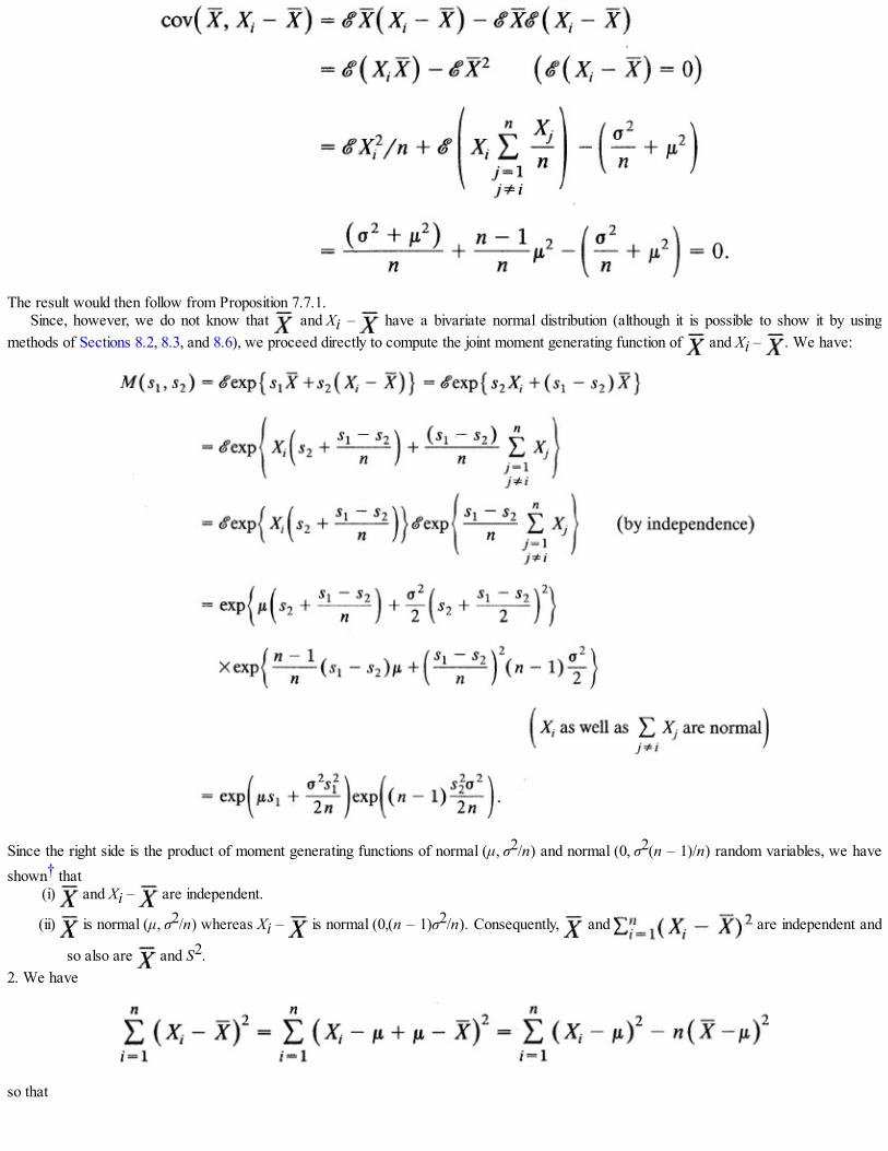
The result would then follow from Proposition 7.7.1.Since, however, we do not know that and Xi – have a bivariate normal distribution (although it is possible to show it by using

methods of Sections 8.2, 8.3, and 8.6), we proceed directly to compute the joint moment generating function of and Xi – . We have:

Since the right side is the product of moment generating functions of normal (μ, σ2/n) and normal (0, σ2(n – 1)/n) random variables, we haveshown† that

(i) and Xi – are independent.

(ii) is normal (μ, σ2/n) whereas Xi – is normal (0,(n – 1)σ2/n). Consequently, and are independent and

so also are and S2.2. We have

so that

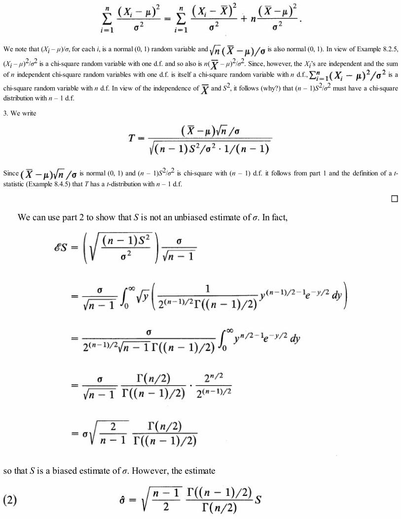
We note that (Xi – μ)/σ, for each i, is a normal (0, 1) random variable and is also normal (0, 1). In view of Example 8.2.5,

(Xi – μ)2/σ2 is a chi-square random variable with one d.f. and so also is n( – μ)2/σ2. Since, however, the Xi’s are independent and the sumof n independent chi-square random variables with one d.f. is itself a chi-square random variable with n d.f., is a

chi-square random variable with n d.f. In view of the independence of and S2, it follows (why?) that (n – 1)S2/σ2 must have a chi-squaredistribution with n – 1 d.f.

3. We write

Since is normal (0, 1) and (n – 1)S2/σ2 is chi-square with (n – 1) d.f. it follows from part 1 and the definition of a t-statistic (Example 8.4.5) that T has a t-distribution with n – 1 d.f.

We can use part 2 to show that S is not an unbiased estimate of σ. In fact,

so that S is a biased estimate of σ. However, the estimate

is unbiased for σ.Let us now consider some properties of t and chi-square densities. We recall (Example 8.4.5) that the

density of t-distribution with n d.f. is given by

Clearly,

so that fn is symmetric about zero. It is unimodal with mode at t = 0. By symmetry, the median is also at t= 0. The existence of mean of fn depends on n. Thus for n = 1,

and f1 does not have finite mean. One can show that |X|r < ∞ for r < n, and in that case all odd-ordermoments vanish. For n > 2, X2 = vai(X) = n/(n – 2). The largest value of fn at t = 0 is

Clearly, fn(t) → 0 as t → ∞ and one can show that as n → ∞ so that fn can be approximated by a standard normal density for

large n. For small n, however, t-distribution assigns more probability to its tails compared with standardnormal distribution.

Table A6 in the Appendix gives the values of tn,α where

for selected values of α and n = 1, 2, …, 30, 40, 60, and 120. Here t(n) has density fn. Thus tn,α is thequantile of order 1 – α. Left tail t values can be obtained by symmetry (Figure 1a). Indeed,

Graphs of fn for some values of n are given in Figure 2.In Tables 1 and 2 we compare t-distribution and standard normal distribution (see also Figure 1b).

Figure 1a

Figure 1b. Comparison of unit normal and t(4) density functions. Reproduced from N. L. Johnson and S.Kotz, Distributions in Statistics: Continuous Univariate Distributions, Vol. 2, Wiley, New York, 1970,

p. 77, with permission.

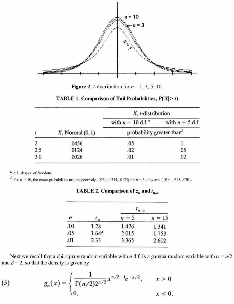
Figure 2. t-distribution for n = 1, 3, 5, 10.

TABLE 1. Comparison of Tail Probabilities, P(|X| > t)

a d.f., degree of freedom.b For n = 10, the exact probabilities are, respectively, .0734, .0314, .0133; for n = 5, they are .1019, .0545, .0301.

TABLE 2. Comparison of zα and tn,α

Next we recall that a chi-square random variable with n d.f. is a gamma random variable with α = n/2and β = 2, so that the density is given by

We note that gn is unimodal for n > 2 and has its maximum (or mode) at x = n – 2. For n = 1 it is strictlydecreasing (with both axes as asymptotes). For n = 2, it is the exponential density with mean 2, and gn isdecreasing with mode† at x = 0. Figure 3 gives graphs of gn for some selected values of n.

We note that for a chi-square (χ2) random variable with n d.f.

Table A7 in the Appendix gives the values of χ2n, α where (Figure 4)

for selected values of α and n = 1, 2, …, 30. Here χ2(n) is a random variable with density gn. For largervalues of n we use the result that has approximately a normal distribution withmean 0, variance 1 (Problem 9.2.7).

Figure 3. Chi-square density for 1, 2, 3, 4, 5 degrees of freedom.

Example 1. Urine Chloride Level in Infants. The mean chloride level in normal infants is assumed to have a normal distribution

with a mean of 210 mEq per 24-hour period. A random sample of six premature infants showed a mean of 203 mEq per 24-hour periodwith a standard deviation of 15 mEq. Is there evidence to suggest that premature infants have a lower urine chloride level?

If X is the mean chloride level in full-term newborn infants, then X has a normal distribution with mean μ = 210 mEq per 24-hourperiod. For the sample n = 6, x = 203 and s = 15. We wish to find P{ ≤ 203|μ = 210}. We have

Figure 4. χn, α2.

For n – 1 = 6 – 1 = 5 d.f. we see from Table A6 that

Therefore, there does not seem to be enough evidence to conclude that premature infants have a lower urine chloride level.What is the probability that the sample comes from a population with standard deviation σ = 10? We need to compute

Here d.f. = n – 1 = 5 so that from Table A7

That is, it is unlikely (the probability is between .02 and .05) that a random sample of size 6 from a normal population with variance σ2 =100 will have a sample variance as large as 225.

In summary, therefore, we have:

L e t X1, X2, …, Xn be a sample from a normal population with mean μ and variance σ2. Let Then,

(i) The statistic has a standard normal distribution,

(ii) and S2 are independent,

(iii) (n – 1)S2/σ2 has a chi-square distribution with (n – 1) d.f., and(iv) has a t-distribution with (n – 1) d.f.

These results can be extended to the case when we have two independent samples. Let X1, X2, …, Xm

and Y1, Y2, …, Yn be two independent random samples from normal populations with parameters μ1, σ21,

and μ2, σ22 respectively. Let X, Y and S2

1, S22 be the corresponding means and variances for the samples.

By the methods of Section 8.6 we can show that

has a standard normal distribution. If σ21, σ2

2 are unknown assume that σ21 = σ2

2 = σ2 (unknown). Then

is an unbiased estimate of σ2 since

Moreover, (m + n – 1)S2/σ2 has a chi-square distribution with (m + n – 2) d.f. This follows (Problem8.6.19) since (m – 1)S2

1/σ2 and (n – 1)S22/σ2 are independent random variables each having a chi-square

distribution. Consequently,

has a t-distribution with m + n – 2 d.f. Moreover, in view of the definition of an F statistic (Example8.4.6), it also follows that:

has an F distribution with (m – 1, n – 1) d.f.We recall that an F random variable with (m, n) d.f. has density function

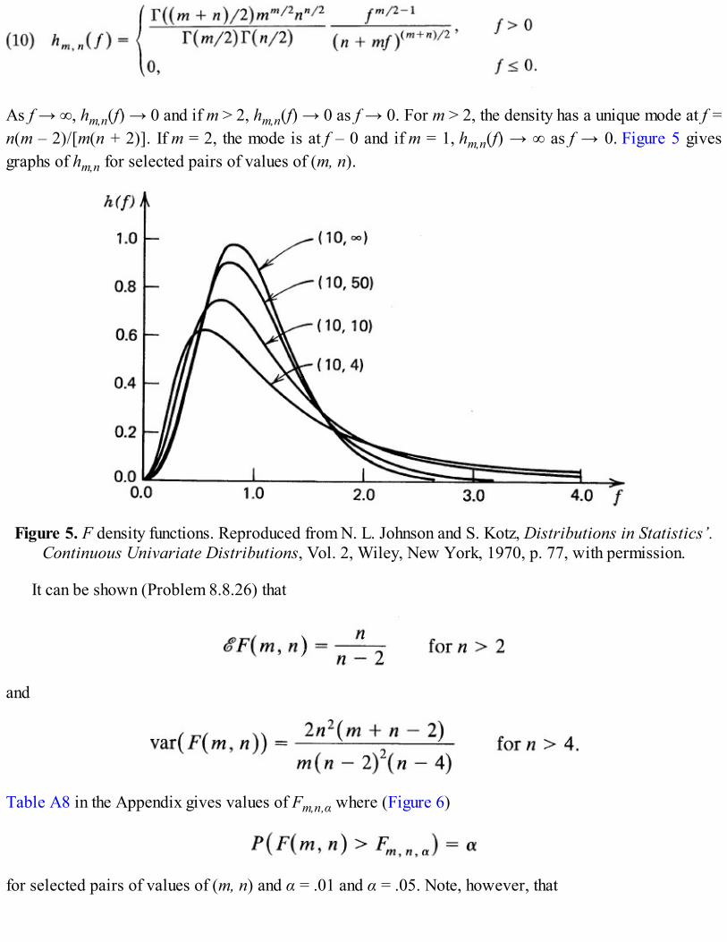
As f → ∞, hm,n(f) → 0 and if m > 2, hm,n(f) → 0 as f → 0. For m > 2, the density has a unique mode at f =n(m – 2)/[m(n + 2)]. If m = 2, the mode is at f – 0 and if m = 1, hm,n(f) → ∞ as f → 0. Figure 5 givesgraphs of hm,n for selected pairs of values of (m, n).

Figure 5. F density functions. Reproduced from N. L. Johnson and S. Kotz, Distributions in Statistics’.Continuous Univariate Distributions, Vol. 2, Wiley, New York, 1970, p. 77, with permission.

It can be shown (Problem 8.8.26) that

and

Table A8 in the Appendix gives values of Fm,n,α where (Figure 6)

for selected pairs of values of (m, n) and α = .01 and α = .05. Note, however, that

so that

Figure 6. Fm, n, α

Consequently,

8.7.1 Confidence Intervals for μ and σ2

We now consider the problem of constructing confidence intervals for μ and σ2 in sampling from a normalpopulation. The results of this section give minimum level 1 – α confidence intervals irrespective of thesize of the sample.

If we want a confidence interval for μ at minimum level 1 – α we have

so that if σ is known, then a confidence interval for μ is

If, on the other hand, σ is unknown, then we replace it by S and we have

since has a t(n – 1) distribution. Hence a (1 – α) level confidence interval for μ is givenby

Confidence Interval for μ

Let X1, X2, …, Xn be a sample of size n from a normal distribution with mean μ and variance σ2.If σ is known

is a minimum level 1 – α confidence interval for μ. If σ is unknown

is a minimum level 1 – α confidence interval for μ.

If μ and σ2 are unknown and a confidence interval for σ2 is desired, we use the fact that (n – 1)S2/σ2

has a χ2 distribution with (n – 1) d.f. Hence given α and n we can find a, b such that

Each such pair (a, b) gives a (1 – α) level confidence interval for σ2, namely,

Since the χ2 distribution is not symmetric we cannot use symmetry to choose a and b (as we did in thecase of computing confidence interval for μ). Although it is possible† to find a and b, numerically, suchthat the length of the confidence interval is minimum, it is simpler to assign equal probability to each tailand choose

Then the equal tails minimum level 1 – α confidence interval for σ2 is given by

Equal Tails Confidence Interval for σ2

(μ unknown).

If μ is known, then one uses

as a (1 – α) level confidence interval for σ2. This follows since (Xi – μ)/σ, for i = 1, 2,…, n areindependent standard normal random variables so that (Xi – μ)2/σ2 is a χ2(1) random variable for each i(Example 8.2.5). By independence their sum is a χ2(n) random variable.

Example 2. Confidence Interval for A verage Length of a Desert Snake. A herpetologist wishes to estimate the length of a rarespecies of desert snake in Nevada. She is able to trap a sample of nine snakes of the species and finds that the mean length is 3.7 feetwith a standard deviation of 1 foot. Find a 90 percent confidence interval for the true mean length of this species of snake assuming thatthe distribution of lengths is normal.

Here x = 3.7, s = 1, and n = 9. Since σ is not known, we use a confidence interval based on t-statistic with n – 1 = 8 d.f. Since α =.10, t8, .05 = 1.860 and a 90 percent confidence interval is given by

We are therefore 90 percent confident that 3.08 ≤ μ ≤ 4.32 in the sense that for about 90 percent random samples of nine snakes of thisspecies the random interval [x – 1.86s/3, x + 1.86s/3] will contain μ.

Example 3. Nicotine Content of a Certain Brand of Cigarettes. The nicotine content of a certain brand of cigarettes measured inmilligrams may be assumed to have a normal distribution. A sample of size 5 produces nicotine contents of 16, 16.5, 19, 15.4, and 15.6.Let us find a 98 percent confidence interval for the average nicotine content of this brand.

Here n = 5, α = .02 so that tn–1, α/2 = t4, .01 = 3.747. Moreover,

and s = 1.459. Hence a 98 percent confidence interval for μ, is given by

We are 98 percent confident that 14.06 ≤ μ ≤ 18.94. If the manufacturer asserts, for example, that the mean nicotine content is 13.5milligram, we will have to be suspicious of his claim, whereas if he claims that μ = 14.5, then the sample does support his claim at level

.02.

Example 4. Variation in Manufacture of Fuses. A random sample of 15 fuses for the 25 amperage value manufactured by acertain company shows a standard deviation of .85 amperage. If the amperage is assumed to be normally distributed, then a 95 percentconfidence interval for σ2 is given by

where n = 15, s2 = (.85)2, α = .05 so that χ214,.025 = 26.119 and χ2

14,.975 = 5.629. The confidence interval is [.39,1.80]. If themanufacturer claims that the variance in amperage of his fuses is .8, we would have to conclude that the sample supports his claim. If aconfidence interval for σ is desired, we take the square root of the above interval. In the example under consideration, a 95 percentconfidence interval for σ is given by [.62,1.34].

Example 5. Sample Size Determination. Suppose we wish to find the sample size n in such a way that the length of the confidenceinterval for μ is fixed in advance at 2d and minimum level at 1 – α. Suppose σ is known. Then

is a 1 – α level confidence interval for μ with length It follows that

If n computed from this formula is not an integer we choose the smallest integer greater than (σ2z2α/2/d2). Often σ is not known. In that

case, we use any prior information on σ that is available, such as the standard deviation from a previous study.In particular, suppose it is desired to find a 95 percent confidence interval for the mean systolic blood pressure of males in such a way

that the length of the confidence interval is 6 mm Hg. Suppose it is known that σ = 10 mm Hg. Then zα/2 = z.025 = 1.96, 2d = 6, and

so that we need a sample of size 43.This problem can be equivalently phrased as follows. It is desired to estimate μ by the sample mean such that the maximum error

is ε with probability 1 – α. What should be n? In that case we want n to satisfy

so that

where Z is standard normal. It follows that

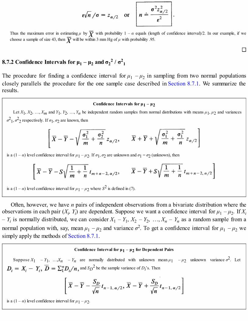
Thus the maximum error in estimating μ by with probability 1 – α equals (length of confidence interval)/2. In our example, if wechoose a sample of size 43, then will be within 3 mm Hg of μ with probability .95.

8.7.2 Confidence Intervals for μ1 – μ2 and σ22 / σ2

1

The procedure for finding a confidence interval for μ1 – μ2 in sampling from two normal populationsclosely parallels the procedure for the one sample case described in Section 8.7.1. We summarize theresults.

Confidence Intervals for μ1 – μ2Let X1, X2, …, Xm and Y1, Y2, …, Yn be independent random samples from normal distributions with means μ1, μ2 and variances

σ21, σ2

2 respectively. If σ1, σ2 are known, then

is a (1 – α) level confidence interval for μ1 – μ2. If σ1, σ2 are unknown and σ1 = σ2 (unknown), then

is a (1 – α) level confidence interval for μ1 – μ2 where S2 is defined in (7).

Often, however, we have n pairs of independent observations from a bivariate distribution where theobservations in each pair (Xi, Yi) are dependent. Suppose we want a confidence interval for μ1 – μ2. If Xi– Yi is normally distributed, we can consider X1 – Y1, X2 – Y2, …, Xn – Yn as a random sample from anormal population with, say, mean μ1 – μ2 and variance σ2. To get a confidence interval for μ1 – μ2 wesimply apply the methods of Section 8.7.1.

Confidence Interval for μ1 – μ2 for Dependent Pairs

Suppose X1 – Y1, …,Xn – Yn are normally distributed with unknown mean μ1 – μ2 unknown variance σ2. Let

and SD2 be the sample variance of Di’s. Then

is a (1 – α) level confidence interval for μ1 – μ2.

To construct a confidence interval for the ratio σ22/σ2

1 in sampling from normal populations (when μ1,μ2 are unknown), we use (9) to find a and b such that

Since the distribution of an F statistic is asymmetric, we use an equal tails approach and choose a = Fm–1,

n–1, 1–α/2 and b = Fm–1, n–1, α/2. Then

Confidence Interval for σ22/σ2

1Let X1, X2, …, Xm and Y1, Y2, …, Yn be independent samples from two normal populations. Then

is a (1 – α) level confidence interval for σ22/σ2

1.

A confidence interval for σ2/σ1 is obtained by taking the square root of the above confidence intervalfor σ2

2/σ21.

Example 6. Confidence Interval for Difference in Performance of Two Groups of Students. A test for reading comprehension isgiven to an elementary school class consisting of 15 Anglo-American and 12 Mexican-American children. The results of the test are asfollows:

Let us compute a 95 percent confidence interval for the difference in means of the two groups assuming that they form random samplesfrom normal populations. In order to apply the confidence interval based on a t-statistic, we need to assume further that σ2

1 = σ22. In thatcase

so that s = 10.43. Also, for α = .05, tm+n–2,α/2 = t25,.025 = 2.06. Hence a 95 percent confidence interval for μ1 – μ2 is given by

We are therefore 95 percent confident that –6.32 ≤ μ1 – μ2 ≤ 10.32. In particular, the evidence suggests that the difference in means is

not significant at the 5 percent level.What about the assumption σ1 = σ2? Let us compute a 90 percent confidence interval for σ2

2/σ21. We note that F14, 11, .05 = 2.74

and Fl4, 11, .95 = 1/F11, 14, .05 = 1/2.56, so that a 90 percent confidence interval is

Since this interval does contain σ22/σ2

1 = 1 our assumption that σ21 = σ2

2 is reasonable.

Example 7. Difference in Birth Weight of Twins. A random sample of six sets of twins was taken, and it showed the followingbirth weights in pounds.

Assuming that the difference in birth weights is a normal random variable, we construct a 98 percent confidence interval for the truedifference in weights of the first-born and the second-born in a set of twins. Here,

S i n c e α = .02, tn– 1 , α/2 = t5, .01 = 3.365, a 98 percent confidence interval is given by In particular, this means that the difference in

mean birth weights of the first-born and second-born twins is not significant at level .02.

8.7.3 Testing Hypotheses Concerning Mean and Difference of Means

In order to test the hypothesis H0: μ = μ0 based on a random sample of size n from a normal population,the appropriate test statistic is

if σ is known and

i f σ is unknown. Clearly, large values of Z (or T) support the alternative H1: μ > μ0 and lead to therejection of H0. Similar arguments apply in the case when H1 is μ > μ0 or μ ≠ μ0. Similar methods alsoapply in the two sample case. We state these results below. It will be shown in Section 11.3 that the sametests are valid when H0 is μ ≤ μ0 or μ ≤ μ0.

Testing Hypotheses Concerning μCompute .

Here T has t distribution with n – 1 d.f. If σ is known, compute instead and usezα instead of tn–l, α.

Due to limitations of the t-tables, the P-value cannot be exactly computed. However, one can getbounds on the P-value.

Testing Hypotheses Concerning μ – μ2 when σ1 = σ2 (unknown)

Compute:

Here T is a t-statistic with m + n – 2 d.f.

If σ1 σ2 are known, then one computes

and uses Zα instead of tm + n – 2, α.We recall that there is a one-to-one correspondence between a size α test of θ = θ0 against θ ≠ θ0 and

a minimum level 1 – α confidence interval for θ. (See Section 4.4.) Hence the confidence intervals ofSection 8.7.1 can be used to accomplish the same purpose and conversely. Similar correspondence exists

between one-sided tests and confidence bounds.

Example 8. Average Handling Costs Per Roll of Film. A mail-order photofinishing company charges 50 per roll as handlingcosts. The manager suspects that handling costs have gone up. In order to verify his hunch he takes a random sample of 16 orders andfinds that the average cost is 55 with a standard deviation of 8 . Suppose the handling cost for an order has a normal distribution. Thenwe wish to test H0: μ = 50 against H1 : μ> 50. We have

and d.f. = 16 – 1 = 15. From Table A6, t15, .01 = 2.602 and t15, .025 = 2.131, so that the P-value satisfies

At level α = .025, we reject H0 and conclude that the observed difference between the sample mean and (μ = 50 is significant. That is,the average handling costs are indeed higher than 50 per roll.

Example 9. Difference in Performance of Two Groups of Students (Example 6). In Example 6 we constructed a 95 percentconfidence interval for the difference in mean scores of Anglo-American students and Mexican-American students. If we wish to testH0: μ1 = μ2 against H1: μ1 ≠ μ2 then under H0: μ1 – μ2 = 0, and since 0 is included in the 95 percent confidence interval [–6.32,10.32]we cannot reject H0 at level .05.

Alternatively, let us compute the value of t0 to see how significant it is. We have

The associated P-value is 2P(T > .495) for 25 d.f. From Table A6 we note that .3 < P(T > .495) < .35 so that t0 is not significant even atα = .60 level.

Example 10. Sample Size Determination. In Example 8, suppose the manager wants to find the size of the sample required toensure that if μ = 50 then he wants no more than 5 in 100 chance of increasing the rate, but if the true average cost is 55 , then he iswilling to raise the charge but is willing to allow a chance of one in 10 of not doing so. Suppose σ = 8.

Here the problem is to test H0: μ = μ0 against H1: μ > μ0 at, say, level α such that the probability of type II error when μ is the truevalue is β. We have, for μ > μ0:

Hence

It follows that

In our case, α = .05, β = .10, σ = 8, μ0 = 50, and μ = 55, so that

Thus the minimum sample size needed is 22.

8.7.4 Testing Hypotheses Concerning Variances

In order to test H0: σ = σ0 against one-sided or two-sided alternatives, the appropriate test statistic is

when μ is unknown, and

when μ, is known. We note that V has a chi-square distribution with n – 1; d.f. whereas V′ has a chi-square distribution with n d.f. Large values of V (or V′) support σ > σ0 and result in rejection of H0 infavor of H1: σ > σ0. A similar test is valid for H0: σ ≥ σ0. We summarize the results below.

Testing Hypotheses Concerning σ2

Compute .

H e r e V is a chi-square random variable with n – 1 d.f. If μ is known, compute and use instead of .

Finally we consider testing H0: σ1 = σ2. In this case the appropriate test statistic is

which, under H0: σl = σ2, reduces to F = S21/S22 and has an F-distribution with (m – 1, n – 1) d.f. Clearly,

large values of F support the claim that σl > σ2 and small values of F support the claim that σ1 < σ2. Thesame tests apply when H0 is σ1 ≤ σ2 or ≥ σ2.

Testing Equality of Variances

Compute f0 = s21/s2

2.

Here F has an F distribution with (m – 1, n – 1) d.f.

The tests can be modified when either or both μ1 or μ2 is known. We leave the reader to furnish thedetails. We emphasize that Table A8 gives only values of Fm, n, α for α = .01 and .05 but does not give lefttail critical values. For this purpose we use the relation (11).

Example 11. Testing Variability in GPA’s of Male and Female Students. In a study of the grade point averages of seniors, aresearcher wishes to use both female and male students. In order to do so she would like to know if the GPAs of male and femalestudents have the same amount of variability. Independent random samples of male and female students gave the following results.

SampleSex Size Standard DeviationFemale 12 3.7Male 17 4.1

Here she wishes to test H0: σ1 = σ2 against H1: σ1 ≠ σ2. We note that

which is in the left tail, so we need Fm – 1, n – 1, 1 – α/2. We have from (11):

Since we do not reject H0 at level .10.

A 90 percent confidence interval for σ22/σ1

2 is easily constructed. It is given by

and that for σ21/σ2

2 is given by [.33,2.20]. Since 1 is included in the interval [.46, 3.01] (or in [.33, 2.20]), we cannot reject H0 at 10percent level of significance.

Remark 1. In the two sample t-test for testing H0: μ1 = μ2 against one-sided or two-sided alternatives,we made the assumption that σ1 = σ2 = σ (unknown). It is therefore tempting to use a pre-test to determinewhether this assumption holds. There are, however, two reasons for not doing so. First, the combinedlevel of significance of an F-test at level α followed by a t-test at level α is no longer α but 1 – (1 – α)2,which is > α. In general, if two tests are performed sequentially, with respective significance levels α1and α2, then the significance level of the combined test is larger than max(α1, α2). Secondly, the F test mayreject H0 not only when H0 is false but also when the underlying distribution is nonnormal. The t-test, onthe other hand, is a good test even when the underlying distribution is only approximately normal.

Remark 2. In Sections 6.3 and 8.5 we studied the sign test for testing hypotheses concerning thequantiles of a distribution or the mean of a continuous symmetric distribution. Thus t-test and sign test arecompetitors for testing hypotheses concerning the mean of a normal distribution. Which of the two testsshould we use? If the underlying distribution is normal, it is intuitively clear that the t-test should bepreferred over the sign test. A more difficult question to answer is, Can we use the t-test even when F isnot normal but unimodal and symmetric? If so, which of the two tests performs better in terms of its powerfunction? Power comparisons are often very difficult to make, especially when the form of F is unknown.In Section 11.5 we consider yet another test for the location parameter of a symmetric distribution. Wealso compare the performance of three tests there. Similar comparisons are made in the two-sample casein Section 11.6.

Problems for Section 8.7

1. Let T have a t-distribution with n d.f. Find:(i) P(|T| < 3.365) if n = 5.(ii) P(|T| > 1.812) if n = 10.(iii) Constant c, if P(|T| ≤ c) = .95, and n = 20.(iv) Constant c, if P(|T| > c) = .10, and n = 12.(v) Constant c, if P(–c < T < 0) = .45, and n = 17.

2. Consider a random sample of size 7 from a normal distribution with mean μ = 18. Let and S2 be thesample mean and the sample variance. Find:(i) P(| – 18| > (1.943/ )S).(ii) P(| – 18| ≤ (1.44/ )S).

Find the constant c such that:(iii) P(| – 18| < cS) = .98.(iv) P(| – 18| > cS) = .20.(v) Estimate P( > 24), P( < 13), and P(12 < < 28) when s = 10.

3. Let X be a chi-square random variable with n d.f. Find:(i) P(X ≤ 2.558) if n = 10.(ii) P(10.600 ≤ X ≤ 21.337) if n = 22.(iii) Constant c, if P(X > c) = .05 and n = 7.(iv) Constant c, if P(X < c) = .01 and n = 9.(v) Constants c1 and c2, if P(X < c1) = P(X > c2) = 05 and n = 10.(vi) Constants c1 and c2, if P(X > c1) = P(X > c2) = .01 and n = 15.

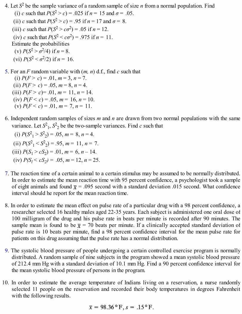
4. Let S2 be the sample variance of a random sample of size n from a normal population. Find(i) c such that P(S2 > c) = .025 if n = 15 and σ = .05.(ii) c such that P(S2 > c) = .95 if n = 17 and σ = 8.(iii) c such that P(S2 > cσ2) = .05 if n = 12.(iv) c such that P(S2 < cσ2) = .975 if n = 11.

Estimate the probabilities(v) P(S2 > σ2/4) if n = 8.(vi) P(S2 < σ2/2) if n = 16.

5. For an F random variable with (m, n) d.f., find c such that(i) P(F > c) = .01, m = 3, n = 7.(ii) P(F > c) = .05, m = 8, n = 4.(iii) P(F > c)= .01, m = 11, n = 14.(iv) P(F < c) = .05, m = 16, n = 10.(v) P(F < c) = .01, m = 7, n = 11.

6. Independent random samples of sizes m and n are drawn from two normal populations with the samevariance. Let S2

1, S22 be the two-sample variances. Find c such that

(i) P(S21 > S2

2) = .05, m = 8, n = 4.(ii) P(S2

1 < S22) = .95, m = 11, n = 7.

(iii) P(S1 > cS2) = .01, m = 6, n – 14.(iv) P(Sl < cS2) = .05, m = 12, n = 25.

7. The reaction time of a certain animal to a certain stimulus may be assumed to be normally distributed.In order to estimate the mean reaction time with 95 percent confidence, a psychologist took a sampleof eight animals and found = .095 second with a standard deviation .015 second. What confidenceinterval should he report for the mean reaction time.

8. In order to estimate the mean effect on pulse rate of a particular drug with a 98 percent confidence, aresearcher selected 16 healthy males aged 22-35 years. Each subject is administered one oral dose of100 milligram of the drug and his pulse rate in beats per minute is recorded after 90 minutes. Thesample mean is found to be = 70 beats per minute. If a clinically accepted standard deviation ofpulse rate is 10 beats per minute, find a 98 percent confidence interval for the mean pulse rate forpatients on this drug assuming that the pulse rate has a normal distribution.

9. The systolic blood pressure of people undergoing a certain controlled exercise program is normallydistributed. A random sample of nine subjects in the program showed a mean systolic blood pressureof 212.4 mm Hg with a standard deviation of 10.1 mm Hg. Find a 90 percent confidence interval forthe mean systolic blood pressure of persons in the program.

10. In order to estimate the average temperature of Indians living on a reservation, a nurse randomlyselected 11 people on the reservation and recorded their body temperatures in degrees Fahrenheitwith the following results.

Find a 95 percent confidence interval for the mean temperature of Indians on this reservation.

11. In Problem 8, suppose the pulse rates of all 16 subjects were recorded before the administration ofthe drug and 90 minutes after the drug, with following results.

Find a 98 percent confidence interval for the mean difference in pulse rates.

12. The copper content of an alloy is normally distributed with variance 7 (percent)2. What is the samplesize required in order to estimate the average copper content by to within 2 percent with 95percent confidence?

13. A random sample of scores on a standardized college entrance examination is to be taken to test H0: μ= 100 against H1: μ < 100 at level α = .10. How large should the sample size be to ensure that theprobability of accepting H0 when μ = 90 is .20? Take σ = 20.

14. The resistance of a wire (in ohms) produced by a manufacturer is normally distributed. In order tocheck if the wires produced on two different machines have the same average resistance (when bothmachines have been set to have same variability), two samples were taken with the following results.

Find a 98 percent confidence interval for the true difference in mean resistances.

15. A random sample of 25 participants in a diet program showed an average weight loss of 6.8 poundsafter the completion of the program. Find a 90 percent confidence interval for the mean decrease inweight of participants in this program, if the sample variance is 3 (pounds)2 assuming that thedifference in weights are normally distributed.

16. In order to estimate with 90 percent confidence the difference in mean monthly income of male andfemale graduates of a university, the Placement Office took two independent random samples ofgraduates (within two months of graduation) with the following results.

What is the confidence interval? Assume population variances are equal.

17. The tar content of two brands of cigarettes is to be compared based on the following sample results:

Is the difference in mean tar content of the two brands significant? At what level?

18. The standard deviation of the fill in a soup-vending machine is important to the vending machineoperator. He takes a random sample of 15 cups and finds that the sample standard deviation is 0.53ounce. Find a 95 percent confidence interval for the true standard deviation of the fill on thismachine.

19. A sample of 16 cigarettes showed a sample mean tar content of 11.2 with a standard deviation of .9.Find a 90 percent confidence interval for the true standard deviation.

20. A phosphate fertilizer was applied to seven plots and a nitrogen fertilizer to five plots. The yield inbushels for each plot was recorded:

Find a 98 percent confidence interval for the ratio σ21/σ2

2 of variances in yields of the two fertilizers.

21. A random sample of 16 half-hour intervals of daytime television programs showed that the mean timedevoted to commercials was 8.5 minutes with a standard deviation of 1 minute. A random sample of10 half-hour prime-time programs showed a mean time of 7.8 minutes with a standard deviation of1.2 minutes. Find a 90 percent confidence interval for the ratio of variances of the two times devotedto commercials.

22. In Problem 7, suppose the psychologist wishes to test that the mean reaction time is no more than .085second, how significant is the observed value of x = .095 second? What would be your conclusion atlevel = .05?

23. In Problem 21, if it is desired to check if there is any difference between the mean time devoted tocommercials during day and prime time programming, how significant is the observed differencebetween the sample means, assuming that σ = σ2? If α = .10, is the difference significant?

24. A manufacturer claims that the average mileage of a particular model it makes equals or exceeds 42miles per gallon. A consumer protection agency conducts a field test with 10 cars of the model, eachof which is run on one gallon of gasoline. The following results were obtained:

Do the data corroborate the manufacturer’s claim at level α = .05? You may assume that the mileageper gallon for this model has a normal distribution. How significant is the observed sample mean?

25. A filling machine is set to fill 2 kg of sugar (when under control). In order to check that the machine isunder control, a random sample of seven bags is selected and their weights recorded:

How strong is the evidence that the machine is out of control?

26. In Problem 11, how strong is the evidence that the administration of the drug reduces the pulse rate by20 beats per minute or more?

27. In Problem 14, how strong is the evidence that the resistance of wires produced on the two machinesare different? What will your conclusion be if α = .05?

28. In Problem 15, is there strong evidence to conclude that the diet program results in a weight reductionof 7.5 pounds or more?

29. In Problem 16, is there evidence to suggest that the mean salary of male graduates exceeds that offemale graduates? Use α = .05.

30. A random sample of 20 American adults showed a mean weight of 162.8 pounds with a standarddeviation of 10.4 pounds. A random sample of 16 Australian adults showed a mean weight of 156.5pounds with a standard deviation of 9.2 pounds. How significant is the difference between the twosample means assuming that σ1 = σ2? Is the difference significant at 5 percent level?

31. Brand A 40-watt bulbs sell for 75¢ each and Brand B bulbs sell for 89$ each. Brand B bulbs claim tohave a higher mean length of life than Brand A bulbs. A random sample of 12 Brand A bulbs showeda mean life length of 2010 hours with a standard deviation of 150 hours. A random sample of 15Brand B bulbs showed a mean life length of 2150 hours with a standard deviation of 165 hours. Dothe data support the claim at level a = .05? Find bounds for the P-value of the observed difference.

32. In Problem 18, the vending machine is considered to be under control if the standard deviation of fillis 0.40 ounces. How strong is the evidence that the machine is not under control? What will be yourconclusion if α = .05?

33. A machine is set to produce flathead wood screws with a variance of .0001 (inch) 2. A random sampleof seven screws showed a sample standard deviation of .016 inch. Would you conclude that themachine is not under control?

34. A jar of peanut butter is supposed to contain an average of 16 ounces with a standard deviation of 1.5ounces. A random sample of 16 jars showed a sample standard deviation of 2.8 ounces. Is itreasonable to conclude that σ > 1.5 ounces?

35. In Problem 14, is it reasonable to conclude that the two machines produce wires whose resistancehave equal variance?

36. In Problem 20, is it reasonable to assume that the yield with nitrogen fertilizer has the same varianceas that with phosphate fertilizer?

37. In Problem 16, is it reasonable to conclude that the monthly income of male graduates is morevariable than that of female graduates?

38. Let X1, X2, …, Xn and Y1, Y2, …, Yn be independent random samples from normal populations withmeans μ1, μ2 and variances σ2

1, σ22 respectively where σi

2, i = 1, 2, are known. It is desired to test H0:μ1 = μ2 against H1: μ1 ≠ μ2 at level α such that the probability of accepting H0 when |μ1 – μ2| = δ is β.What should the minimum sample size be? In particular, if α = β = .05, σ1 = σ2 = 4, and δ = 1, find n.

8.8 REVIEW PROBLEMS

1. Suppose X is a random variable with distribution function F. Define:

and

(i) Show that the distribution function of X+ is given by:

and that of X– by

(ii) In particular, if X is a standard normal random variable show that X+ is a mixed type randomvariable with distribution given by

(iii) If X has a uniform distribution in [– 1, 1], show that X+ has distribution given by

2. Suppose X has density function f(x) = 2x/π2 for 0 < x < π, and zero elsewhere. Show that Y = sin X hasdensity given by

3. Suppose X has density function f and distribution function F. Let Y = g(X) be defined as follows:

(i) g(x) = 1 if x > 0, and = –1 if x ≤ 0,(ii) g(x) = x if |x| ≥ c, and = 0 if |x| < c, where c is a constant, c > 0,(iii) g(x) = c if x ≥ c, = x if |x| < c, and = – c if x ≤ – c, where c > 0 is a constant.In each case find the distribution of Y.

4. Let X1, X2 be a random sample from a standard normal distribution. Let S2 be the sample variance.

(i) Show that S2 has a chi-square distribution with 1 d.f. [Hint: S2 = (X1 – X2)2/2. Use Problem 8.6.20or prove directly that (X1 – X2)/ has a standard normal distribution. Then use Example 8.2.5 or8.3.3. For the general case, see Section 8.7.]

(ii) Show that X1 + X2 and X1 – X2 are independent. Hence conclude that and S2 are independent.

5. Suppose X has uniform distribution on (0,1). Find the function h such Y = h(X) has the distributiongiven by

(i) P(Y = y)= p(1 – p)y–1, y = l, 2, …(ii)

(iii) fY(y) = 1 /y2, y ≥ 1, and zero elsewhere.(iv) fY(y) = 3y2, 0 < y < 1, and zero elsewhere.(v) fy(y) = y if 0 < y < l, = 2 – y if 1 ≤ y < 2, and zero otherwise.

6. Suppose X1, X2 is a random sample from an exponential distribution with mean λ. Show that X1 + X2and X1/X2 are independent random variables. Hence conclude that X1 + X2 and X1/(X1 + X2) are alsoindependent. [Hint: Show that P(X1 + X2 ≤ u, X1/X2 ≤ v) = P(X1 + X2 ≤ u) · P(Xl/X2 ≤ v) for all u, v.]

7. Let X1 be the total time between a customer’s arrival at a service station and his departure from theservice desk. Let X2 be the time spent in line before reaching the service desk. Suppose (X1, X2) havea joint density function given by

Show that the service time Y = X1 – X2(≥0) has density function given by

8. Suppose X and Y are independent random variables and k ≥ 0 is a fixed nonnegative integer. Find thedistribution of Z = X + Y + k for the following cases:(i) When X is binomial (m, p) and Y is binomial (n, p).(ii) When X is Poisson with mean λ and Y is Poisson with mean μ.In each case find the mean and the variance of Z.

9. A foot ruler is broken into two pieces at a point chosen at random. Let Z be the ratio of the length ofthe left piece to the length of the right piece. Show that Z has density function

What is the probability that the length of the longer piece is larger than twice the length of the shorterpiece?

10. In Problem 9 find the density of the ratio (length of the longer piece/length of the shorter piece).

11. Let X and Y be tensile strengths of two kinds of nylon fibers and suppose that X and Y are independentwith common density function

Find the density function of Z = X + Y. (See also Example 3.4.3.)

12. Suppose X, Y, Z, U have joint density function

and zero elsewhere. Find the density function of X + Y + Z + U. (See also Problem 3.4.15.)

13. Let X1, X2 be a random sample from density function f given below. Find the density function of Z =min(X, Y)/max(X, Y).(i) f(x) = 6x(1 – x), 0 < x < 1, and zero otherwise.(ii) f(x) = xe–x, x > 0, and zero otherwise.

14. Let X1, X2, …, Xn be a random sample from the uniform distribution on (0, 1) and let X(1) < … < X(n)be the set of order statistics. Show that

15. Suppose X1, X2 is a random sample from a normal distribution with mean μ, and variance σ2.(i) Show that

Thus is an unbiased estimate of σ. Find var( ).(ii) Show that so that is an unbiased estimate of σ.

16*. Suppose X has a normal distribution with mean μ and variance σ2. Show that Y = X2 has the densityfunction given by

and zero otherwise.

17. Suppose X1, X2, …, Xn is a random sample from a Poisson distribution with mean λ.

(i) Find the conditional distribution of Xk given .(ii) Show that the joint conditional distribution of X1, X2, …, Xn given X1 + … + Xn = t is

multinomial.

18. Suppose X has a Poisson distribution with mean λ and c is a constant. Show that(i) {cX exp(–cX)} = λc exp{λ(e–c – 1) – c}.(ii) exp(–cX) = exp{–λ(1 – e–c)}.

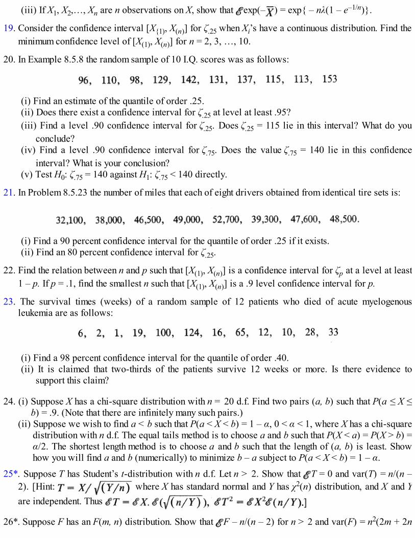
(iii) If X1, X2,…, Xn are n observations on X, show that exp(– ) = exp{ – nλ(1 – e–1/n)}.

19. Consider the confidence interval [X{1), X(n)] for ζ.25 when Xi’s have a continuous distribution. Find theminimum confidence level of [X(1), X(n)] for n = 2, 3, …, 10.

20. In Example 8.5.8 the random sample of 10 I.Q. scores was as follows:

(i) Find an estimate of the quantile of order .25.(ii) Does there exist a confidence interval for ζ.25 at level at least .95?(iii) Find a level .90 confidence interval for ζ.25. Does ζ.25 = 115 lie in this interval? What do you

conclude?(iv) Find a level .90 confidence interval for ζ.75. Does the value ζ.75 = 140 lie in this confidence

interval? What is your conclusion?(v) Test H0: ζ.75 = 140 against H1: ζ.75 < 140 directly.

21. In Problem 8.5.23 the number of miles that each of eight drivers obtained from identical tire sets is:

(i) Find a 90 percent confidence interval for the quantile of order .25 if it exists.(ii) Find an 80 percent confidence interval for ζ.25.

22. Find the relation between n and p such that [X(1), X(n)] is a confidence interval for ζp at a level at least1 – p. If p = .1, find the smallest n such that [X(1), X(n)] is a .9 level confidence interval for p.

23. The survival times (weeks) of a random sample of 12 patients who died of acute myelogenousleukemia are as follows:

(i) Find a 98 percent confidence interval for the quantile of order .40.(ii) It is claimed that two-thirds of the patients survive 12 weeks or more. Is there evidence to

support this claim?

24. (i) Suppose X has a chi-square distribution with n = 20 d.f. Find two pairs (a, b) such that P(a ≤ X ≤b) = .9. (Note that there are infinitely many such pairs.)

(ii) Suppose we wish to find a < b such that P(a < X < b) = 1 – α, 0 < α < 1, where X has a chi-squaredistribution with n d.f. The equal tails method is to choose a and b such that P(X < a) = P(X > b) =α/2. The shortest length method is to choose a and b such that the length of (a, b) is least. Showhow you will find a and b (numerically) to minimize b – a subject to P(a < X < b) = 1 – α.

25*. Suppose T has Student’s t-distribution with n d.f. Let n > 2. Show that T = 0 and var(T) = n/(n –2). [Hint: where X has standard normal and Y has χ2(n) distribution, and X and Yare independent. Thus

26*. Suppose F has an F(m, n) distribution. Show that F – n/(n – 2) for n > 2 and var(F) = n2(2m + 2n

– 4)/[m(n – 2)2(n – 4)] for n > 4. (Hint: F = (X/m) (n/Y) where Xand Y are independent chi-square random variables, etc.)

27. If T has a t-distribution with n d.f., show that T2 has an F distribution with (1, n) d.f. (Nocomputations are required.)

28. Let X1, X2, …, X12 be a random sample from a normal population with mean 0 and variance 9.(i) Find (ii) Find

29. The average birth weight of all infants in the United States is Y pounds. In order to study the effect ofthe mother’s diet on the birth weight of her infant, a random sample of 12 pregnant mothers was takenand the mothers were put on a diet beginning the 12th week of pregnancy. The sample mean birthweight of their infants was recorded to be 6.4 pounds with a standard deviation of 1.12 pounds. Didthe diet have an effect on infants’ birth weight?

30. Suppose the systolic blood pressure of all males is normally distributed. A random sample of sevenmales showed an average systolic blood pressure of 122.7 mm Hg with a standard deviation of 21.8mm Hg.(i) Find a 90 percent confidence interval for the true mean systolic blood pressure.(ii) Find a 95 percent confidence interval for the standard deviation of systolic blood pressure.(iii) Is the observed average systolic blood pressure in the sample significantly different from the

national average of 120 mm Hg?(iv) Is the observed sample standard deviation significantly different from the standard deviation σ =

20 mm Hg for the population of all males?

31. Two groups of experimental animals were run through a maze independently under differentconditions. The respective sample means and sample standard deviations of the times it took to run themaze were recorded as follows:

(i) Is the difference between the two group means significant?(ii) Find a 98 percent confidence interval for the difference in means.(iii) Is the difference between the two standard deviations significant?

32. In order to the difference in grades in mathematics on a standardized test for two high schools,independent random samples of students were selected from each school and the test wasadministered with the following results:

(i) Is the difference between the two standard deviations significant?(ii) Find a 90 percent confidence interval for σB/σA, the ratio of two standard deviations. Also find a

98 percent confidence interval for σB/σA.(iii) Is the difference between the two grades significant?

† Alternatively, one could use the relation between beta and binomial distributions (Example 7.5.2) to obtain

Differentiate with respect to x to get (8).†One could instead take [x] to be the smallest integer greater than or equal to x. In that case †R. E. Johnson and E. S. Kiokemeister, Calculus with Analytic Geometry, 5th ed., Allyn and Bacon, Boston, 1974, p. 450.†See Problem 8.6.22(ii).†Mode at x = 0 if we define gn(x) at x = 0 by the first equality in (5).†See Problem 8.8.24.

CHAPTER 9

Large-Sample Theory

9.1 INTRODUCTION

We have seen that in any problem of statistical inference the choice of a statistic, though very important, isonly the first step. In actual application of a test of hypothesis (or in the construction of a confidenceinterval) we also need to compute the P-value (or the numerical limits of the confidence interval). Inorder to do so we need to know the exact distribution of the test statistic.

Suppose, for example, that we wish to estimate the mean age at which married women have their firstchild in a large city. A random sample of n such women shows a mean age of 24.8 years. We have seenthat = 24.8 is a good estimate of the mean age. How good is this estimate? Its precision as measured byits variance is given by σ2/n where σ2 can be estimated from the sample. What if we want a 95 percentconfidence interval for μ, the unknown mean? We will need to know the distribution of . If theunderlying distribution of the Xi’s is known, we may be able to compute the distribution of by methodsof Sections 8.3, 8.4, or 8.6. Given the distribution of it is at least theoretically possible to find a and bsuch that

In order to find a confidence interval for μ, we then have to be able to invert the inequality a ≤ ≤ b inthe form l( ) ≤ μ ≤ u( ).

In practice it may be either difficult or inconvenient to find the distribution of . Even if a and b areknown it may be inconvenient to invert a ≤ ≤ b in the form l( ) ≤ μ ≤ u( ) to give a 1 – α levelconfidence interval for μ.

We need therefore to investigate some alternative approach to find the numerical limits of theconfidence interval. One possible approach is to approximate the distribution of . If the approximatingdistribution is nice enough and the approximation is good enough, then it may be possible to compute aand b with the help of a table of probabilities such as normal or t-distribution.

In this chapter we consider the special case when the sample size n is large. By the law of largenumbers we know that is likely to be near μ (that is, consistent for μ) when n is large. We will showthat when var(X) = σ2 is finite we can closely approximate the distribution of by a normal distributionwith mean μ and variance σ2/n. This so-called central limit theorem is proved in Section 9.3. It is basic toall large sample theory of statistical inference. In Section 9.4 we improve upon the normal approximationin the special case when the population being sampled is (discrete) integer valued. In Section 9.5 weconsider the concept of consistency of an estimate (first introduced in Section 4.3) in some detail.Sections 9.6, 9.7, and 9.8 deal with the estimation and testing of hypothesis for means, proportions andquantiles. In Section 9.9 we return to the problem of testing whether the data can be fit by a specific(known) distribution.

Section 9.2 deals with the general problem of approximating the distribution of a statistic. The reader

may skip this section and the proof of the central limit theorem given in Section 9.3, at least on a firstreading. Neither is crucial to the understanding of other sections or subsequent chapters. It is important,however, to learn the application of the central limit theorem and its ramifications as explained inSections 9.3, 9.6, 9.7, and 9.8.

9.2 APPROXIMATING DISTRIBUTIONS: LIMITING MOMENTGENERATING FUNCTION

Approximating the probability of an event is an important part of statistics. Indeed, all the stochasticmodels studied in this book are approximations in that the assumptions underlying the model may not bestrictly correct and yet it may often give reasonably satisfactory representation. In any event, it is astarting point from which departures may be measured.

Yet another type of approximation is needed when we wish to compute probabilities involving acomplicated statistic. Even if we know the distribution of the statistic, the computation involved may betedious. For example, if X has a binomial distribution with parameters n and p, it is often difficult tocompute

when n is very large, say 500. Similarly, if X1, X2, …, Xn are independent round-off errors in n numbers,then we can assume that each Xi has uniform distribution on (–1/2, 1/2). What is the probability that thetotal error will exceed n/4? In this case, the distribution of the total error can becomputed (although the computation is not easy—see Example 9.3.2), but it is a formidable task tocompute P(Sn > n/4) exactly since the density of Sn is quite complicated. Often one simply does not knowthe exact distribution of the statistic.

Let X1, X2, …, Xn be a sample from a distribution function F. Suppose we wish to find pn = P(T(X1,X2, … Xn) ∈ A) for some set A on the real line. If this cannot be done exactly and simply for any of thereasons outlined above, we should like to approximate pn. This can be done if we can approximate thedistribution of T(X1, X2, …, Xn) by some known and simpler distribution F. In that case we can simplyapproximate pn by the probability that F assigns to the set A.

Examples of this kind have already appeared in Chapter 6, where we approximated (under certainconditions) binomial by Poisson, hypergeometric by binomial, and so on.

In simple mathematical terms the problem is as follows: Let Tn = T(X1, X2, …, Xn), and Fn(x) = P(Tn≤ x) for n ≥ 1. Does there exist a distribution function F such that Fn → F as n → ∞? If so, then for(sufficiently) large n we can replace Fn by F. The following property of moment generating functions isfrequently useful in finding F the limiting distribution function of Fn.

THEOREM 1. (CONTINUITY THEOREM). Let Tn be a random variable with moment generatingfunction Mn, n = 1, 2, …. Let T be a random variable with moment generating function M and supposethat Mn, M are finite for |s| < s0, s0 > 0 and all n. If for every |s| < s0

then

for each x ∈ at which F is continuous. (Here Fn is the distribution function of Tn.)The proof of Theorem 1 is beyond the scope of this text and is omitted. We consider some examples.

Example 1. Two-Point Distribution. Let Xn have probability function

Then for s ∈

for all s ∈ . Since M(s) = 1 is the moment generating function of random variable X degenerate at 0, we conclude from Theorem 1 that

(The point x = 0 is not a continuity point of F(x) = P(X ≤ x) = 0 if x < 0, = 1 if x ≥ 0.) The result also holds at x = 0 since P(Xn ≤ 0) = 1 –1/n → 1 = P(X ≤ 0).

Example 2. Poisson Approximation to Negative Binomial. Let X have probability function

then X has a negative binomial distribution. The probability P(X = k + r), is the probability of the rth success on the (k + r)th trial in asequence of independent Bernoulli trials with constant probability p of success on each trial. The moment generating function of X is givenby

which is finite for s < –ln(1 – p). Taking logarithms and expanding into a Taylor series, we have for s < –ln(1 – p):

Let p → 1 and r → ∞ such that r(1 – p) → λ > 0. Then

and it follows that

Since eλ(es – 1) is the moment generating function of the Poisson distribution with mean λ, it follows from Theorem 1 that the negativebinomial distribution can be approximated by the Poisson distribution for large r, largep, and λ = r(l – p).?

Example 3. Normal Approximation to Poisson. Let X have probability function

where λ < 0 and X = var(X) = λ. Consider the standardized X, defined by

we have for s ∈

so that

Letting λ → ∞ we see that

and it follows from Theorem 1 that the distribution of Z can be approximated by a standard normal distribution for large λ. That is, forlarge λ, X has approximately a normal distribution with mean λ and variance. λ?

Example 4. Borel Weak Law of Large Numbers. Let X1, X2, … be independent and identically distributed Bernoulli random

variables with parameter p, 0 < p < 1. Let and consider the sequence n–1Sn. We have

Hence

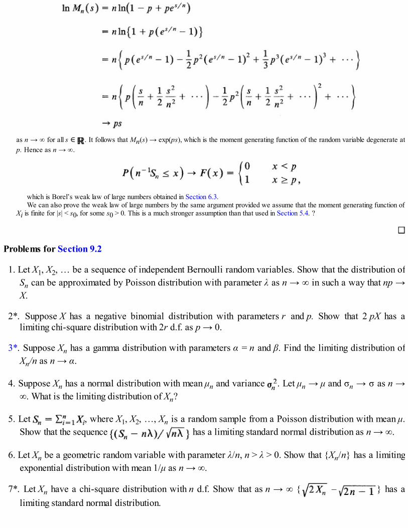
as n → ∞ for all s ∈ . It follows that Mn(s) → exp(ps), which is the moment generating function of the random variable degenerate atp. Hence as n → ∞.

which is Borel’s weak law of large numbers obtained in Section 6.3.We can also prove the weak law of large numbers by the same argument provided we assume that the moment generating function of

Xi is finite for |s| < s0, for some s0 > 0. This is a much stronger assumption than that used in Section 5.4. ?

Problems for Section 9.2

1. Let X1, X2, … be a sequence of independent Bernoulli random variables. Show that the distribution ofSn can be approximated by Poisson distribution with parameter λ as n → ∞ in such a way that np →X.

2*. Suppose X has a negative binomial distribution with parameters r and p. Show that 2 pX has alimiting chi-square distribution with 2r d.f. as p → 0.

3*. Suppose Xn has a gamma distribution with parameters α = n and β. Find the limiting distribution ofXn/n as n → α.

4. Suppose Xn has a normal distribution with mean μn and variance . Let μn → μ and σn → σ as n →∞. What is the limiting distribution of Xn?

5. Let , where X1, X2, …, Xn is a random sample from a Poisson distribution with mean μ.Show that the sequence has a limiting standard normal distribution as n → ∞.

6. Let Xn be a geometric random variable with parameter λ/n, n > λ > 0. Show that {Xn/n} has a limitingexponential distribution with mean 1/μ as n → ∞.

7*. Let Xn have a chi-square distribution with n d.f. Show that as n → ∞ { – } has alimiting standard normal distribution.

8. Suppose X1, X2, …, Xn, … is a sequence of independent Bernoulli random variables with parameterp. Show that has an approximate normal distribution with mean np and variance np(1– p) for sufficiently large n. [Hint: Consider .]

9. An estimate is required of the difference in proportions of male and female students who have a gradepoint average of 3.5 or better at a large university. A sample of n students is taken from thepopulation of students who have a grade point average of 3.5 or better. If Y is the number of malestudents in the sample, then (2Y/n) – 1 is a good estimate of p1 – p2 where p1 is the true proportion ofmale students with 3.5 or better grade point average. Show that (2Y/n) – 1 has an approximate normaldistribution with mean p1 – p2 = 2p1 – 1 and variance 4p1(1 – p)/n = 4p1p2/n for large n. [Hint: UseProblem 8.]

9.3 THE CENTRAL LIMIT THEOREM OF LEVY

We now demonstrate the key role played by the normal distribution in probability and statistics. The mainresult of this section is the central limit theorem due to Levy (Theorem 1) which says that the distributionof the sum of n independent identically distributed (nondegenerate) random variables with finite variancecan be approximated by the normal distribution provided the sample size n is sufficiently large. Tomotivate the central limit theorem, we first consider some examples.

Example 1. Sample Size Required to Estimate μ with Prescribed Error. Let X1, X2, …, Xn be a random sample from a population

with mean and (finite) variance σ2. Let We know that = n–1Sn is unbiased for μ and has variance σ2/n.Moreover, the weak law of large numbers tells us that

so that for large n, is likely to be close to μ. Hence is a candidate as an estimate for μ. Suppose we estimate μ, by and want toensure that the error | – μ| in estimation is no more than ε > 0 with a probability of, say, at least 1/2. How large should the sample sizebe? In other words, we want to find n such that

In the particular case when the Xi’s have a normal distribution, the solution is simple. It was given in Example 8.7.5. We choose n tosatisfy

In the nonnormal case, however, we can apply the Chebyshev’s inequality to choose n. Indeed,

(with ); on comparing (2) and (4) we see that

It is clear that n given by (5) is much larger than that given by (3). Is (5) the best we can do in the nonnormal case? We will see that even

in this case n given by (3) suffices.

Example 2*. Magnitude of Round-off Error. In Example 7.2.1 we saw that the uniform distribution may be used to model round-off error. Suppose n numbers are rounded off to the nearest integer. Let X1, X2, …, Xn be the round-off errors. Then X1, X2, … Xn areindependent identically distributed random variables with uniform distribution on [–1/2, 1/2]. The total round-off error is given by

. What is the probability that the round-off error is more than n/4? That is, what is P(Sn > n/4)? If fn is the density ofSn, then

Let us compute fn. Since Sn = Xn + Sn–1, n ≥ 2, we have from (8.4.5)

for x ∈ [–n/2, n/2] where we have used the fact that f1(y) = 1 for y ∈ [–1/2, 1/2] and f1(y) = 0 otherwise. Let us write

Then we can rewrite

using the convention 0° = 0. Using (6) with n = 2 we have (see Figure 1)

We can rewrite f2 in terms of δ as follows

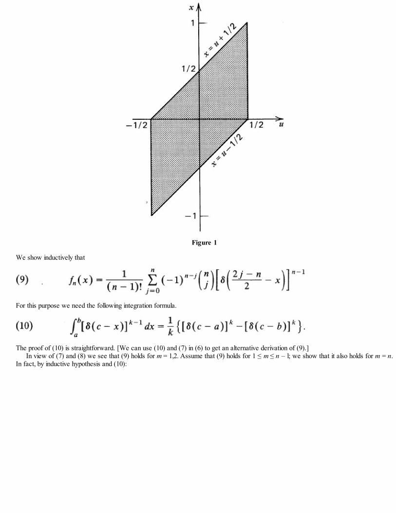
Figure 1

We show inductively that

For this purpose we need the following integration formula.

The proof of (10) is straightforward. [We can use (10) and (7) in (6) to get an alternative derivation of (9).]In view of (7) and (8) we see that (9) holds for m = 1,2. Assume that (9) holds for 1 ≤ m ≤ n – l; we show that it also holds for m = n.

In fact, by inductive hypothesis and (10):

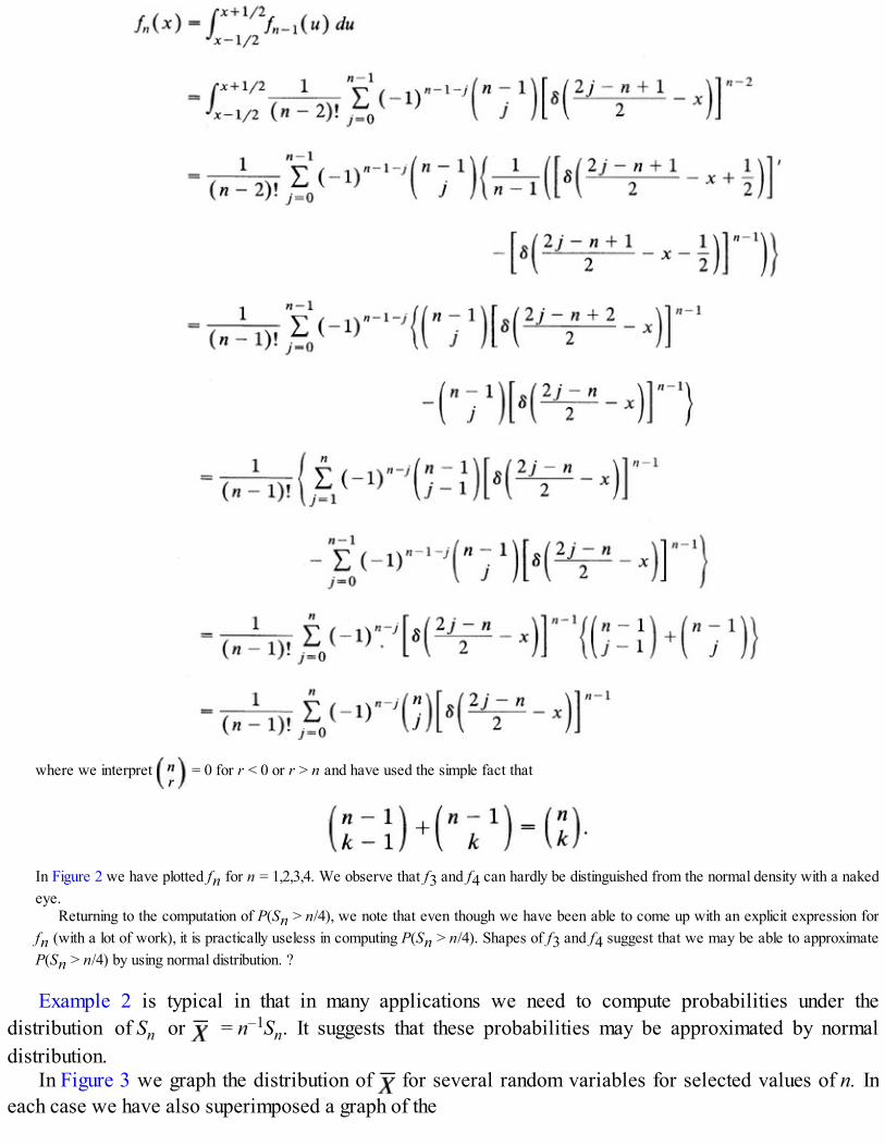
where we interpret = 0 for r < 0 or r > n and have used the simple fact that

In Figure 2 we have plotted fn for n = 1,2,3,4. We observe that f3 and f4 can hardly be distinguished from the normal density with a nakedeye.

Returning to the computation of P(Sn > n/4), we note that even though we have been able to come up with an explicit expression forfn (with a lot of work), it is practically useless in computing P(Sn > n/4). Shapes of f3 and f4 suggest that we may be able to approximateP(Sn > n/4) by using normal distribution. ?

Example 2 is typical in that in many applications we need to compute probabilities under thedistribution of Sn or = n–1Sn. It suggests that these probabilities may be approximated by normaldistribution.

In Figure 3 we graph the distribution of for several random variables for selected values of n. Ineach case we have also superimposed a graph of the

Figure 2. Graphs of fn [given by (9)] for n = 1,2,3,4.

Figure 3 a. Distribution of for binomial (5, p = .3) random variables.

Figure 3b. Distribution of for Poisson random variables with mean 3.

Figure 3C. Distribution of for exponential random variables with mean 1.

normal curve with the same mean (= μ) and same variance (= σ2/n). In each case the two curves are rathersimilar for larger values of n, and agreement improves as n gets larger.

Let us now explore the possibility of approximating the distribution of by normal distribution. Notethat if P(Xi > 0) = 1, then Xi = μ, > 0, P(Sn > 0) = 1 so that P(Sn ≤ x) = 0 for x ≤ 0. Moreover, P(| – μ|> ε) → 0 so that for large n, Sn “behaves like” nμ. In particular, Sn → ∞.†“ We cannot, therefore, expectP(Sn ≤ x) to converge to the normal distribution (see Section 9.2). The case when Xi’s have a normaldistribution with mean μ and variance σ2 suggests that we need to “adjust” Sn suitably. In Section 8.7 wesaw that Z = [ ( – μ)]/σ = (Sn – nμ) / σ has an exact normal distribution. This is simply thestandardized or Sn.

Following the normal case, let us consider the standardized sums

Clearly Zn = 0 and var(Zn) = 1. We show that P(Zn ≤ x) → as n → ∞. That is,we can approximate the distribution of Zn by standard normal distribution.

THEOREM 1. (LÉVY’S CENTRAL LIMIT THEOREM). Let {Xn} be a sequence of nondegenerateindependent identically distributed random variables with common mean μ and common variance σ2, 0< σ2 < ∞. Let , n = 1,2,…, and Zn = . Then for all z ∈

Proof.* A complete proof of Theorem 1 is beyond the scope of this text. We restrict ourselves to the casewhen Xn’s have a moment generating function M(s) which is finite in |s| < s0 for some s0 > 0. (This, inparticular, implies that |Xj|k > ∟ for all k, which is considerably more than what we are given in thestatement of the theorem.) For ease in writing and for computational convenience, we assume without lossof generality‡ that μ = 0 and σ = 1. Then

We need to show (in view of the continuity theorem of Section 9.2) that

Taking logarithms, we have

Set ϕ(x) = In M(x). Then

We note that ϕ(0) = In M(0) = ln 1 = 0. Clearly ϕ is differentiable (Section 8.6). By L’Hôpital’s rule

Again ϕ′(0) = Xi = μ = 0 (by (8.6.18)) so that the conditions for L’Hôpital’s rule are again satisfied. Wehave

by continuity of ϕ″. In view of (8.6.18), ϕ′(0) = var(Xi) = σ2 = 1 and it follows that

Since exp(s2/2) is the moment generating function of a standard normal random variable, it follows fromthe continuity theorem (Theorem 9.2.1) that

which is (11).

Remark 1. Theorem 1 is a remarkable result. It says that the limiting distribution of the standardized

partial sums is standard normal irrespective of the distribution of the random variables being summedprovided the variance is finite.

Remark 2. We can write (11) in terms of . Indeed,

where

Remark 3. According to (11) for large n,

That is Sn is approximately (or asymptotically) normally distributed with mean nμ and variance nσ2.Similarly, is approximately normally distributed with mean μ and variance σ2/n. Often we will say thatXn is asymptotically normal to mean that, when standardized, Xn has a limiting standard normaldistribution.

Remark 4. How large must n be before we can apply the approximation? What is the error in thisapproximation? Both these questions concern the speed of convergence of P(Zn ≤ x) to ϕ(x). That is, therate of convergence of |P((Sn – nμ)/σ ≤ x) – ϕ(x)| to zero. Clearly, the rate of convergence shoulddepend on the distribution of the Xi’s. If Xi’s have a symmetric distribution to begin with, one wouldexpect the approximation to be good even for moderately large n. The following estimate of error innormal approximation appears to be the best result known so far. If |(Xi, – μ)/σ|3 < ∞ then

Table 1 gives the error bound for some common distributions.It is wise to use caution in using normal approximation. Although the error estimate in (12) can

frequently be used to show that the error in approximation is not too large, it should be emphasized thatthis estimate gives a bound for any distribution F for which μ, σ and |Xk – μ|3 is all that is known.Needless to say that (12) can be improved in special cases when F is completely specified.

Remark 5. The weak law of large numbers tells us that converges to μ (in the sense that P(| – μ| >ε) → 0 as n → ∞). By Chebyshev’s inequality

so that the rate of convergence is that of n–1. The central limit theorem, on the other hand, gives a moreprecise estimate of the rate of convergence. Indeed, for large n

in view of Problem 7.6.24.

Remark 6. According to Chebyshev’s inequality

whereas according to central limit theorem

for large n, which may be thought of as a refinement of (14) in that (15) provides a much more preciseestimate. (See Table 7.6.1 for a comparison.)

Example 3. Breakdown of a Machine; Normal Approximation to Gamma Distribution. The times between breakdowns of amachine can be modeled as an exponential random variable with mean λ with density

TABLE 1. Error Bound for Some Common Distributions

Let X1, X2, …, Xn be a random sample from f so that X1 is the waiting time for the first breakdown, X2 for the second breakdown, and soon. Then is the total time to the nth breakdown. What is P(Sn > t), the probability that the nth breakdown does notoccur before time t? We recall (Problem 8.6.19) that Sn has a gamma distribution with parameters α = n and β = λ. Hence

and in view of Example 7.4.4 we have

Given n, t, and λ we can compute this probability by using a table of Poisson probabilities.Note that X1 = λ and var(X1) = λ2 so that for large n we can apply the central limit theorem. We have

which can be read off from a table of normal distribution.In particular let λ = 2 months, n = 30, and t = 36. Then the exact probability from a table of cumulative Poisson probabilities with λ =

18 is given by

Normal approximation gives

with error |.9941 – .9857| = .0016, which is very small even though n is not very large. (The error bound from Table 1 gives .0301 but theactual error .0016 is much less.)

How large should n be such that

From normal approximation

so that

Solving for n, we get (choosing the larger root):

In the particular case when λ = 1, t = 36, and α = .95, z.05 = 1.645 and we have

The exact probability for n = 48 is given by P(Sn > 36) = .968 so that the approximation is quite satisfactory.

Example 4. Sample Size Determination (Example 1). In Example 1 we wanted to choose n such that the estimate of μ has amaximum error of ε with probability ≥ 1/2. Thus we choose n to satisfy

By central limit theorem

so that from Table A5 we choose n satisfying

which is much smaller than the one suggested by Chebyshev’s inequality. In particular, let Xi be Bernoulli random variables with p = .30and let ε = .05. In that case Chebyshev’s inequality requires that we choose n according to (5), that is,

The normal approximation requires only that we choose

which is considerably smaller. For comparison purposes let us compute the exact value of n from binomial tables. We have

Here Sn has a binomial distribution with parameters n (unknown) and p = .3. By trial and error and using a more comprehensive binomialtable than Table A3 (such as the Harvard University Table), we get n = 32.

Example 5. Round-Off Error (Example 2). We return to the problem of Example 2 where we wish to compute the probability thattotal round-off error in rounding off n numbers exceeds n/4. Since each Xi is uniform on [–1/2,1/2], μ = Xi = 0 and σ2 = var(Xi) = 1/12.By central limit theorem Sn is asymptotically normally distributed with mean 0 and variance n/12. Consequently,

which can be computed once n is given.Suppose n = 1000 and we want P(Sn > 25). Then

In this case we cannot compare our result with the exact probability since we cannot integrate f1000 as given in (9). Table 1 gives theerror in normal approximation to be at most 1.036/ = 1.036/ = .0328, quite large in relation to the magnitude of the probabilitybeing estimated. The actual error in normal approximation is in fact much smaller in this case, but we do not propose to investigate it anyfurther.

Example 6. Conviction Rate. In a very large city it is known that about 0.1 percent of the population has been convicted of a crime.What is the probability that in a random sample of 100,000 from this population, at most 120 have been convicted of a crime?

Let X be the number in the sample who have been convicted of a crime. Then X has a binomial distribution with n = 100,000 and p =.001 so that

We consider X as the sum of n = 100,000 independent identically distributed random variables Xi, each with parameter p = .001. Then

and

Since X = 100 is large, it is inconvenient to apply the Poisson approximation (6.6.3). By the central limit theorem, however,

The error bound from Table 1 is

which is not very precise. What if we have to estimate a small probability, such as P(X = 120)? First note that we cannot apply the centrallimit approximation directly to P(X = 120) since it will lead to the approximation P(X = 120) 0 (Why?). Let us write

Then

Now the error bound is practically meaningless.

I n Section 9.4 we consider some further approximations and also a correction that leads to animprovement in normal approximation when applied in the special case when the Xi’s are integer valued.

The central limit theorem holds also in the case when the Xi’s are independent but not necessarilyidentically distributed. Extensions to random vectors is also known, but we will not pursue the subjectany further. We conclude this section with the following simple application of the central limit theorem.

Example 7. Normal Approximation to Poisson and an Application. Let X1, X2, …, Xn be a random sample from a Poissondistribution with mean λ. Then has a Poisson distribution with parameter nλ. Since Sn = var(Sn) = nλ it followsthat?

In particular, let λ = 1 and x = 0. Then

Since Sn has a Poisson distribution with parameter n, however,

It follows that

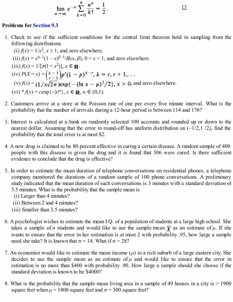
Problems for Section 9.3

1. Check to see if the sufficient conditions for the central limit theorem hold in sampling from thefollowing distributions.

(i) f(x) = 1/x2, x ≥ 1, and zero elsewhere.(ii) f(x) = xα–1(1 – x)β–1/B(α, β), 0 < x < 1, and zero elsewhere.(iii) f(x) = 1/[π(l + x2)], x ∈ .(iv) P(X = x) = .

(v) f(x) = , and zero elsewhere.(vi) * f(x) = cexp{–|x|α}, x ∈ , α ∈ (0,1).

2. Customers arrive at a store at the Poisson rate of one per every five minute interval. What is theprobability that the number of arrivals during a 12-hour period is between 114 and 176?

3. Interest is calculated at a bank on randomly selected 100 accounts and rounded up or down to thenearest dollar. Assuming that the error in round-off has uniform distribution on (–1/2,1 /2), find theprobability that the total error is at most $2.

4. A new drug is claimed to be 80 percent effective in curing a certain disease. A random sample of 400people with this disease is given the drug and it is found that 306 were cured. Is there sufficientevidence to conclude that the drug is effective?

5. In order to estimate the mean duration of telephone conversations on residential phones, a telephonecompany monitored the durations of a random sample of 100 phone conversations. A preliminarystudy indicated that the mean duration of such conversations is 3 minutes with a standard deviation of3.5 minutes. What is the probability that the sample mean is

(i) Larger than 4 minutes?(ii) Between 2 and 4 minutes?(iii) Smaller than 3.5 minutes?

6. A psychologist wishes to estimate the mean I.Q. of a population of students at a large high school. Shetakes a sample of n students and would like to use the sample mean as an estimate of μ. If shewants to ensure that the error in her estimation is at most 2 with probability .95, how large a sampleneed she take? It is known that σ = 14. What if σ = 28?

7. An economist would like to estimate the mean income (μ) in a rich suburb of a large eastern city. Shedecides to use the sample mean as an estimate of μ and would like to ensure that the error inestimation is no more than $400 with probability .90. How large a sample should she choose if thestandard deviation is known to be $4000?

8. What is the probability that the sample mean living area in a sample of 49 houses in a city is > 1900square feet when μ = 1800 square feet and σ = 300 square feet?

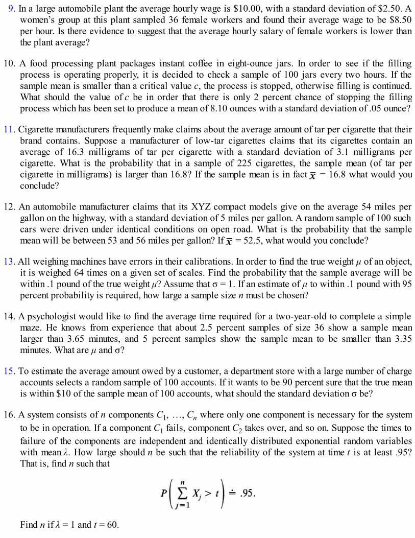
9. In a large automobile plant the average hourly wage is $10.00, with a standard deviation of $2.50. Awomen’s group at this plant sampled 36 female workers and found their average wage to be $8.50per hour. Is there evidence to suggest that the average hourly salary of female workers is lower thanthe plant average?

10. A food processing plant packages instant coffee in eight-ounce jars. In order to see if the fillingprocess is operating properly, it is decided to check a sample of 100 jars every two hours. If thesample mean is smaller than a critical value c, the process is stopped, otherwise filling is continued.What should the value of c be in order that there is only 2 percent chance of stopping the fillingprocess which has been set to produce a mean of 8.10 ounces with a standard deviation of .05 ounce?

11. Cigarette manufacturers frequently make claims about the average amount of tar per cigarette that theirbrand contains. Suppose a manufacturer of low-tar cigarettes claims that its cigarettes contain anaverage of 16.3 milligrams of tar per cigarette with a standard deviation of 3.1 milligrams percigarette. What is the probability that in a sample of 225 cigarettes, the sample mean (of tar percigarette in milligrams) is larger than 16.8? If the sample mean is in fact = 16.8 what would youconclude?

12. An automobile manufacturer claims that its XYZ compact models give on the average 54 miles pergallon on the highway, with a standard deviation of 5 miles per gallon. A random sample of 100 suchcars were driven under identical conditions on open road. What is the probability that the samplemean will be between 53 and 56 miles per gallon? If = 52.5, what would you conclude?

13. All weighing machines have errors in their calibrations. In order to find the true weight μ of an object,it is weighed 64 times on a given set of scales. Find the probability that the sample average will bewithin .1 pound of the true weight μ? Assume that σ = 1. If an estimate of μ to within .1 pound with 95percent probability is required, how large a sample size n must be chosen?

14. A psychologist would like to find the average time required for a two-year-old to complete a simplemaze. He knows from experience that about 2.5 percent samples of size 36 show a sample meanlarger than 3.65 minutes, and 5 percent samples show the sample mean to be smaller than 3.35minutes. What are μ and σ?

15. To estimate the average amount owed by a customer, a department store with a large number of chargeaccounts selects a random sample of 100 accounts. If it wants to be 90 percent sure that the true meanis within $10 of the sample mean of 100 accounts, what should the standard deviation σ be?

16. A system consists of n components C1, …, Cn where only one component is necessary for the systemto be in operation. If a component C1 fails, component C2 takes over, and so on. Suppose the times tofailure of the components are independent and identically distributed exponential random variableswith mean λ. How large should n be such that the reliability of the system at time t is at least .95?That is, find n such that

Find n if λ = 1 and t = 60.

17. From a table of random numbers, one-digit numbers are selected from 0,1, …, 9 (repetitionsallowed). Let Sn be the sum of numbers in n selections. Approximate the probabilities for large n:(i) P(Sn ≥ 4.55n). (ii) P(Sn ≤ 4.52n).Take n = 625, 2500, 10,000, 40,000, 62,500. What is the limit in each case as n → ∞?

18*. Extend the result in Example 7 and show that for λ > 0

(The case λ = 1 is proved in Example 7.)

19*. Use the central limit theorem to show that

[Hint: Consider the sum of independent exponential random variables with mean 1.]

20*. Let X1, X2, …, Xn be independent identically distributed random variables with common uniformdistribution on (0,1). Imitate the proof in Example 2 to show that has density function

where ε(x) = 0, if x ≤ 0, and = x if x ≥ 0.

21. Let X1, X2, … be a sequence of independent random variables with common mean μ1 and variance .Let {Yn} be a sequence of independent random variables with common mean μ2 and variance andsuppose that {Xn} and {Yn} are independent. Show that – has an asymptotic normal distributionwith mean μ1 – μ2 and variance ( + )/n. [Hint: Consider the sequence Zn = Xn – Yn, n ≥ 1.]

22. In Problem 21 suppose that the sequences {Xn} and {Yn} are dependent and cov(Xn, Yn) = ρσ1σ2 forall n. What is the asymptotic distribution of – ?

23. (i) Specialize Problem 21 to the case when {Xn} is a sequence of independent Bernoulli randomvariables with parameter pl and {Yn} is an independent sequence of Bernoulli random variableswith parameter p2, {Xn} and {Yn} are independent.

(ii) Specialize part (i) to the case when (Xn, Yn) have a multinomial distribution with parameters n, p1and p2.

24. Let {Xn} be a sequence of independent identically distributed random variables such that |Xn|2k < ∞.Write , Show that is asymptotically normally distributed with mean and variance .

25*. Suppose X1, X2, … are independent identically distributed with Xi = 0 and 0 < .Show that

for large n and any e > 0. [Hint: Use Problem 7.6.24.]

9.4† THE NORMAL APPROXIMATION TO BINOMIAL, POISSON, ANDOTHER INTEGER-VALUED RANDOM VARIABLES

We restrict attention to the case when the random variables Xn take only integer values 0,1,2, …. Thisincludes, for example, binomial, Poisson, hypergeometric, and negative binomial random variables.According to the central limit theorem, has approximately a normal distribution with meann Xi = and variance n var(Xi) = nσ2 for large n. In Section 9.3 we gave a bound for the error in thisapproximation and showed that the error is sometimes large. We suggest some alternative approximationsand a correction that leads to a somewhat better approximation.

We note that the central limit theorem concerns the convergence of distribution functions (of Sn’s) andnot probability or density functions (to the normal density function). Suppose first that the Xn’s are of thecontinuous type. Then Sn is also a continuous type random variable [this follows, for example, from(8.2.5)] with density function fn. By the central limit theorem for large n

where μ = Xi, σ2 = var(Xi) and ϕ is the standard normal distribution function.If we differentiate both sides of (1) with respect to x we get

A formal justification of (2) will not be given here but (2) provides a good approximation for large n.(We also need the condition that fn is bounded for some n.) A result such as (2) is called a local centrallimit theorem as against (1), which is a global result. A similar result holds also in the discrete case. Weassume that the Xi’s have positive probability only over the set of integers k = 0, ± 1, ± 2,…. Then thefollowing result holds.

as n → ∞ where x is of the form (k – nμ)/σ for k = 0, ± 1, ± 2,…. That is, for sufficiently large n

Example 1. Early Births: Another Approximation for Binomial Probability. Suppose the Xn’s are Bernoulli random variables so

that Sn is a binomial random variable with parameter p, 0 < p < 1. Since μ = Xi = p, σ2 = var(Xi) = p(1 – p), we have, for large n

for k = 0,1,…In a recent study of births it was found that about 1/3 of the births arrived earlier than the doctor had predicted. What is the probability

that in 100 randomly selected births exactly 35 will arrive earlier than predicted? Let X be the number of early arrivals. According to (5),P(X = 35) .0795. The exact probability from Table A3 is .0763.

If we want P(X ≤ l) we simply add the right side of (5) for k = 0,1,…,l.

Example 2. Breakdowns of a Machine (Example 9.3.3). We consider once again the times X1, X2, …, Xn between breakdownsof a machine where each Xi has an exponential distribution with mean λ < 0. Then Sn has a gamma density given by

According to (2) we can approximate fn, for large n, by

Figure 1. Binomial probabilities for n = 50, p = .4 and normal approximation (5).

The true probability or density functions of Examples 1 and 2 and the corresponding normalapproximations (5) and (6) are plotted in Figures 1 and 2.

From Figure 1 we arrive at yet another method for approximating P(Sn = k) in the discrete (integervalued) case which is usually more accurate than the original normal approximation formula (9.3.11)given by the central limit theorem or even (4). Indeed, from (4),

k = 0,1,2,…. The area of the shaded region in Figure 1 is an approximation to P(Sn = k). The idea is thatwe are approximating the area under the histogram for the distribution of Sn by the normal curve.Summing over k from k = 0 to k = x, say, we are led to the approximation

Figure 2. Gamma density with n = 25; λ = 3 and normal approximation(6)

where x is an integer ≥ 0. This is usually more accurate than the approximation

This approximation procedure is referred to as continuity correction and applies for all integer valuedrandom variables such as binomial, Poisson, geometric, and hypergeometric.

Remark 1. The continuity correction helps to improve the accuracy of the central limit theoremapproximation in all cases where the random variable X being sampled has a discrete distribution onequally spaced points. A random variable that takes only values k + lh, l = 0, ± 1, ± 2,… with positiveprobability is known as a lattice random variable. Continuity correction should be applied for all latticerandom variables by writing, for example,

where t is a possible value of . The approximation (3) [or (4)] also holds for lattice randomvariables.

Example 3. Early Births: Normal Approximation to Binomial with Continuity Correction (Example 1). Suppose we wish to findthe probability of at most 35 early births in a sample of 100 births. Then

The exact probability from Table A4 is .7054, so the error is about 4 percent. If the continuity correction is not applied, then

and the error is about 10 percent. Also,

which is a better approximation than the one provided by (5).

Example 4*. Reversal in an Election: Normal Approximation to Hypergeometric. In Example 6.4.6 we computed the probabilityof reversal in an election with two candidates A and B by applying the binomial approximation to hypergeometric distribution. We recallthat if A gets a votes and B get b votes, a > b, and n votes are invalid, then the number of invalid votes for A is a hypergeometric randomvariable with distribution

The probability of reversal is given by P(X ≥ (n + a – b)/2).Since hypergeometric distribution can be approximated by binomial and binomial by normal, we will approximate the probability of

reversal by normal distribution. (A formal proof is too complicated to bother with here.)We recall that

Hence

where Z is a standard normal random variable. It is possible to simplify the expression for z considerably. First we note that

so that

since when a + b is large we can replace a + b – 1 by. Now

so that

It follows that

Hence

for large a + bIn the particular case of Example 6.4.6 we have n = 75, a = 510, b = 490, so that

as compared with .0158 obtained by applying binomial approximation.The reader may justifiably wonder why we went through so much trouble to simplify the probability of reversal when a

straightforward standardization and application of the central limit theorem (or binomial approximation) leads to practically the same result.Apart from the fact that we may not have the binomial probabilities available for the desired n and p, the approximation

has a slight advantage. It tells us that the desired probability depends primarily on the plurality a – b and the number of invalid votes n.The total number of votes cast is much less important since 1/(a + b) is nearly zero for large a + b. Thus given α, 0 < α < 1, where

a – b and n are related according to (a – b)2 nz2α.

Example 5. Salk Polio Vaccine. In 1954 a large field trial was conducted in the United States to test the effectiveness of the Salkvaccine as a protection against polio. The following table summarizes the results.

The null hypothesis to be tested was that treatment has no effect, that is, the vaccine offered no protection. Under the null hypothesis,therefore, we wish to test that the proportions of children who contracted polio is the same in the two groups, the treatment group and thecontrol group. Under H0 we can think of a lot of N = 401,974 children of which D = 148 are marked polio and the remaining N – D =401,826 are marked “no polio.” A random sample of size n = 200,745 is selected as the treatment group. Then the number X of these whohave polio is a random variable with a hypergeometric distribution. According to the Fisher-Irwin test of Section 6.4, we reject H0 if X is

small. The P-value associated with the observation 33 is PH0(X ≤ 33). Since n is large and D/n = 148/401,974 = 3.68 X 10–4 is very

small, we use the normal approximation. We have

and

so that

where � is the standard normal distribution function. Thus, the probability of observing as small as 33 cases of polio in random samplingunder the null hypothesis is less than one in 100 million. There is little or no support for H0 and we have every reason to conclude that theSalk vaccine does indeed offer protection from polio.

Remark 2. Examples 4 and 5 indicate that normal approximation can also be used to evaluateprobabilities in sampling without replacement from a finite population. The following result holds. Let{X1, X2, …, Xn} be a random sample from a finite population of size N with mean μ and variance σ2.Then, as n → ∞ and N/n → ∞ the sequence

has a limiting standard normal distribution.We recall (Example 5.3.1) that = μ, var( ) = σ2(N – n)/[n(N – 1)] where (N – n)/(N – 1) is the

finite population correction. When n/N is small (< .05) we can use var( ) σ2/n. Hypergeometricdistribution is the special case when P(Xi = 1) = D/N and P(Xi = 0) = (N – D)/N.

Remark 3. According to (8)

If n is so large that

we can drop the continuity correction since Table A5 gives probabilities under the normal curve only atjumps of .01. (We are assuming that a number x, N.005 ≤ x < N.01 will be rounded off to N.01.) If σ = 1,for example, this means that for n > 10,000 we can drop the continuity correction.

Remark 4. Often the approximation is applied to . If t is a possible value of , then the continuitycorrection approximation for P( ≤ t) is given by

Alternatively, we can translate the statement in terms of and apply the continuity correction. Forexample, let = = Y/n be the proportion of successes in n trials. Let n = 100 and suppose we want P(≤ .45) when p = .5. Then

since .45 is a possible value of . If n = 84, say, and we want P( ≤ .45) when p = .5, then we note that.45 is not a possible value of . In this case we write

and use (8) to obtain

We have seen that frequently there are several approximations to choose from. When should weapproximate binomial by Poisson and when should we apply normal approximation to binomial? In Table1 we summarize various approximations and provide guidelines to help in this choice. In applications ofthe central limit theorem we will often be required to compute probabilities such as P( ≥ ε) without anyknowledge of the underlying distribution (other than knowledge of σ2 or s2 and the sample size n). In thatcase we will approximate the required probability by using normal approximation as long as n isgreater than or equal to 30. Thus the phrase “large n” in this context means n ≥ 30.

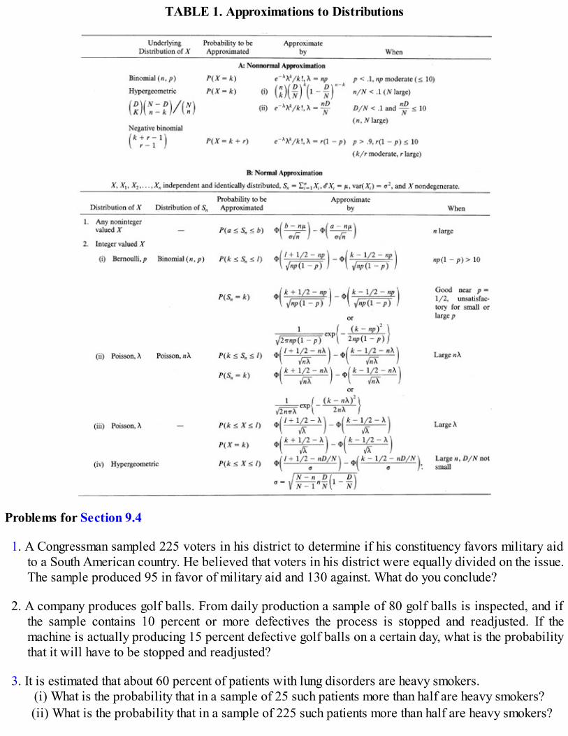
TABLE 1. Approximations to Distributions

Problems for Section 9.4

1. A Congressman sampled 225 voters in his district to determine if his constituency favors military aidto a South American country. He believed that voters in his district were equally divided on the issue.The sample produced 95 in favor of military aid and 130 against. What do you conclude?

2. A company produces golf balls. From daily production a sample of 80 golf balls is inspected, and ifthe sample contains 10 percent or more defectives the process is stopped and readjusted. If themachine is actually producing 15 percent defective golf balls on a certain day, what is the probabilitythat it will have to be stopped and readjusted?

3. It is estimated that about 60 percent of patients with lung disorders are heavy smokers.(i) What is the probability that in a sample of 25 such patients more than half are heavy smokers?(ii) What is the probability that in a sample of 225 such patients more than half are heavy smokers?

4. A bag of 500 half-dollars is dumped at the counter of a local utility company by an irate consumer toprotest the large bill she got from the company for the month of February. What is the probability thatbetween 225 and 250 (both inclusive) half-dollars showed heads? Find the probability that fewerthan 100 showed heads.

5. According to genetic theory, when two right varieties of peas are crossed, the probability of obtaininga smooth seed is 1/2. An experimenter would like to be 95 percent certain of having at least 50 seedsthat are smooth. How many seeds must she produce?

6. A multiple-choice test consists of 75 questions, with five choices for each answer, one of which iscorrect. Assume that a student answers all questions by pure guessing. What is the expected numberof correct answers? What is the probability that the first four answers are correct? What is theprobability that at least 20 answers are correct? Suppose each correct answer carries one point andeach incorrect answer carries zero points. In order to eliminate the effect of guessing, how manypoints should be taken off for an incorrect answer so that the long-run score per question will average0 points?

7. Candidate X believes that he can win a countywide election if he can poll at least 53 percent of thevotes in the city which is the seat of the county. He believes that about 50 percent of the county’svoters favor him. If 6150 voters show up to vote in the city, what is his chance of winning? What if2500 vote in the city?

8. A state legislator in a certain state wishes to assess voters’ attitudes in her district to determine if thevoters favor repeal of the Equal Rights Amendment that the state legislature had passed a year ago.Polls show that the sentiment in the state is about 60 percent against repeal. If she were to select arandom sample of 80 voters from her district, what is the probability that a majority of the samplewould be against repeal? If it is found that only 45 percent in the sample are against repeal, whatwould you conclude?

9. A fair coin is tossed until the first head is observed. The number of trials is recorded. This experimentis repeated n times. Let Sn be the total number of trials required for n successes. What should n be sothat the probability is .05 that the total number of trials needed is at least t? Find n when t = 500.(Note that Sn has a negative binomial distribution. Use the relation in Section 6.5 between a binomialand a negative binomial distribution to find n.)

10. In the peak period of an outbreak of flu it is assumed that about .1 percent of the people in a city havethe bug. In a sample of 10,000 people, what is the probability that 15 will have the flu? Estimate thesame probability for a sample of 62,500.

11. It is estimated that the probability that a baby will be born on the date the obstetrician predicts is1/40. What is the probability that of 400 babies born 15 will be born on the date the doctor predicts?Use Poisson as well as normal approximations.

12. Let X(t) be the number of customers that enter a store in interval (0, f) and suppose X(t) has a Poissondistribution with parameter μt where λ = 50 per hour. Find the smallest t such that

13. A random sample of 50 swimmers is taken at a swim meet with 450 participants consisting of 200girls and 250 boys. Estimate the probability that the number of girls in the sample is:

(i) Greater than or equal to 30.(ii) Between 20 and 25 (inclusive).(iii) Larger than 30.

14. There are 500 participants at a convention of physicians. A random sample of size 60 is taken. Let be the sample average income in thousands of dollars. Find the probability that:

(i) ≥ 67,(ii) < 68,(iii) 62 < < 66,if it is known that μ = 65, σ = 10.

15. Consider a finite population of N weights of pigs at a farm. To estimate the mean weight of pigs on thefarm to within ε pounds with probability at least 1 – α, 0 < α < 1, a sample of size n is to be taken andthe sample mean is to be used to estimate μ. How large should n be if the standard deviation ofweights of pigs is known to be σ pounds?

16. Let X(t) be the number of telephone calls that come in to a service counter switchboard in t minutes. IfX(t) has a Poisson distribution with parameter 5t, find the probability that in a five-hour period therewill be:

(i) Less than 1500 calls.(ii) More than 1600 calls.(iii) Between 1500 and 1550 calls.

17. A machine produces, under normal operations, on the average 1 percent defectives. Approximate theprobability that in 100 items produced by the machine there will be 2 or more defectives. Comparethe Poisson and normal approximations to the exact probability from Table A3 under appropriateindependence assumption.

18. The number of automobile accidents on a two-day weekend at a particular traffic intersection can bemodeled by a Poisson distribution with mean 3. The number of accidents at this intersection isrecorded for all the 52 weeks of the year. Find the probability that the average number of accidentson nonholiday weekends (assume there are 45 nonholiday weekends in a year) at this intersectionwill be:

(i) Greater than 4.(ii) Less than 2.5.(iii) Between 2.8 and 3.5 (inclusive).

19. A town has 5000 voters of which 60 percent are Republicans and 40 percent Democrats. A randomsample of 100 voters is taken. Approximate the probability that the sample contains exactly 50Democrats. Use binomial as well as normal approximations.

9.5 CONSISTENCY

We consider once again a desirable property of estimates first introduced in Section 4.3. Suppose we

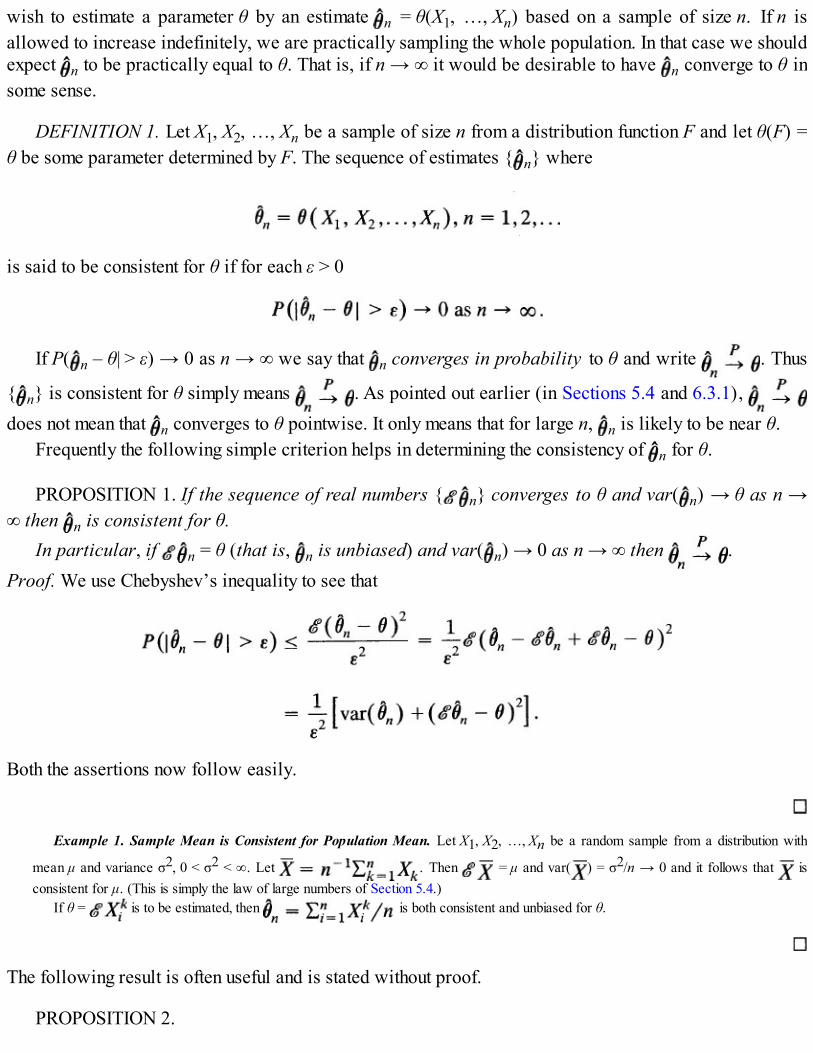
wish to estimate a parameter θ by an estimate n = θ(X1, …, Xn) based on a sample of size n. If n isallowed to increase indefinitely, we are practically sampling the whole population. In that case we shouldexpect n to be practically equal to θ. That is, if n → ∞ it would be desirable to have n converge to θ insome sense.

DEFINITION 1. Let X1, X2, …, Xn be a sample of size n from a distribution function F and let θ(F) =θ be some parameter determined by F. The sequence of estimates { n} where

is said to be consistent for θ if for each ε > 0

If P( n – θ| > ε) → 0 as n → ∞ we say that n converges in probability to θ and write . Thus

{ n} is consistent for θ simply means . As pointed out earlier (in Sections 5.4 and 6.3.1), does not mean that n converges to θ pointwise. It only means that for large n, n is likely to be near θ.

Frequently the following simple criterion helps in determining the consistency of n for θ.

PROPOSITION 1. If the sequence of real numbers { n} converges to θ and var( n) → θ as n →∞ then n is consistent for θ.

In particular, if n = θ (that is, n is unbiased) and var( n) → 0 as n → ∞ then .Proof. We use Chebyshev’s inequality to see that

Both the assertions now follow easily.

Example 1. Sample Mean is Consistent for Population Mean. Let X1, X2, …, Xn be a random sample from a distribution with

mean μ and variance σ2, 0 < σ2 < ∞. Let . Then = μ and var( ) = σ2/n → 0 and it follows that isconsistent for μ. (This is simply the law of large numbers of Section 5.4.)

If θ = is to be estimated, then is both consistent and unbiased for θ.

The following result is often useful and is stated without proof.

PROPOSITION 2.

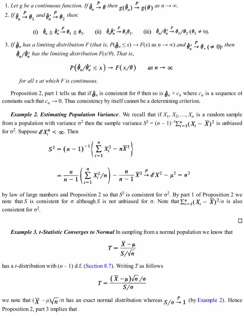
1. Let g be a continuous function. If then as n → ∞.

2. If and then:

3. If n has a limiting distribution F (that is, P( n ≤ x) → F(x) as n → ∞) and , then has the limiting distribution F(x/θ). That is,

for all x at which F is continuous.

Proposition 2, part 1 tells us that if n is consistent for θ then so is n + cn where cn is a sequence ofconstants such that cn → 0. Thus consistency by itself cannot be a determining criterion.

Example 2. Estimating Population Variance . We recall that if X1, X2,…, Xn is a random samplefrom a population with variance σ2 then the sample variance S2 = (n – 1)–1 is unbiasedfor σ2. Suppose . Then

by law of large numbers and Proposition 2 so that S2 is consistent for σ2. By part 1 of Proposition 2 wenote that S is consistent for σ although S is not unbiased for σ. Note that /n is alsoconsistent for σ2.

Example 3. t-Statistic Converges to Normal In sampling from a normal population we know that

has a t-distribution with (n – 1) d.f. (Section 8.7). Writing T as follows

we note that ( – μ) /σ has an exact normal distribution whereas (by Example 2). HenceProposition 2, part 3 implies that

as n → ∞.If Xi’s are not necessarily normally distributed but have a finite variance σ2 and then the

central limit theorem implies the same result.

Example 4. Empirical Distribution Function As a Consistent Estimate. Let X1, X2, … Xn be arandom sample from a distribution function F. We recall that the empirical distribution function of thesample is defined by

Let Y = Y(x) = number of Xi’s ≤ x. Then Y has a binomial distribution with parameters n and p = p(x) =P(Xi ≤ x) = F(x). It follows from Example 1 that

for each x ∈ .

Example 5. The Taxi Problem . In Example 6.2.5 we considered X(n) = Mn = max(X1, …, Xn) as anestimate of N, the total number of taxis in a town. It is intuitively clear that Mn is consistent for N. In fact,for ε > 0,

Since ε > 0, [N – ε]/N < 1 as well as (N – ε – 1)/N < 1 so that

Hence Mn is consistent for N. Moreover the estimate 1 = [(n + 1)/(n)]Mn is also consistent for N.

Problems for Section 9.5

1. (i) Let Y be the number of successes in n Bernoulli trials with parameter p. Show that Y/n, theproportion of successes is consistent for p.

(ii) Show, with = Y/n, that has approximately a standard normaldistribution for large n.

2. Suppose X1 and X2 are the number of successes in n1 and n2 trials respectively. Show that 1 – 2 isconsistent for p1 – p2 where i = Xi/ni, i = 1,2.

3. Let p1 be the proportion of male students at a state university and p2 that of female students. Anestimate of p1 – p2, the excess proportion of males over females, is required. Find a consistentestimate for p1 – p2 and find the limiting distribution of your estimate. [Hint: p1 = 1 – p2]

4. Show that (X/n)2 and X(X – 1)/n(n – 1) are both consistent estimates of p2 where X is the number ofsuccesses in n trials with constant probability p of success.

5. (i) Find a consistent estimate of λ in sampling from a Poisson distribution with parameter λ.(ii) Find a consistent estimate of P(X = 0) = e–λ.

6. Let X1, X2, …, Xn and Y1, Y2, …, Yn be independent random samples from two populations with meansμ1 and μ2 and variances and respectively.

(i) Show that – is consistent for μ1 – μ2.(ii) * If σ1 = σ2 = σ, and , show that

is consistent for σ2.(iii) Show that is asymptotically normal with mean 0 and variance 1.

7. Let X1, X2, …, Xn be a random sample from a geometric distribution with parameter p. Find aconsistent estimate for p.

8. Let X1, X2, …, Xn be a random sample from a population with mean μ and variance σ2. Which of thefollowing estimates are consistent for μ

(i) 1 = (X1 + X2 + … + Xn)/(n/2).(ii) 2 = .(iii) 3 = {(X1 + X2 + … + X[n/2])/[n/2]}, ([x] is the largest integer ≤ x).(iv) 4 = X1.

9. Which of the following estimates are consistent for variance?

(i) = (X1 – X2)2/2.(ii) .(iii) , where 2 is as defined in Problem 8(ii).

10. Let X1, X2, … Xn, be a random sample from the uniform distribution on (0, θ). Which of the followingestimates are consistent for θ?

(i) 1 = 2 .(ii) 2 = [(n + l)/n]max(X1, …, Xn).(iii) 3 = max(X1, …, Xn).(iv) 4 = (n + 1)R/(n – 1) where R = max(X1, X2, …, Xn) – min(Xl, X2, … Xn).(v) 5 = X1 + (X2 + … + Xn)/(n – 1).

11. Let { n} be any sequence of estimates for θ. We say that n is mean square consistent for θ, if and | n – |2 → 0 as n → ∞.

(i) Show that mean square consistency implies consistency.(ii) Show that { n} is mean square consistent if and only if var( n) 0 and n → θ as n → ∞. ( n

→ θ is known as asymptotic unbiasedness of n. n – θ → 0 can also be written as bias of n

→ 0.) [Hint: Use Chebyshev’s inequality and the fact that ( n – θ)2 = var( n) + ( n – 0)2.]

12. Let X1, X2, …, Xn be a random sample from the uniform distribution on (θ, θ + 1). Show that 1 = –1/2 and 2 = max(X1, …, Xn) – n/(n + 1) are both consistent for 0.

13. Let X1, X2, …, Xn be a random sample from density function

Is consistent for θ?

14. Let X1, X2, …, Xn and Y1, Y2, …, Yn be independent random samples from populations with variances and respectively. Find consistent estimates of

(i) / .(ii) /( + ).(iii) .

(You may assume that .)

15. Let X1, X2, …, Xn be a random sample from the uniform distribution on (0, θ). Show that is consistent for θ/e. [Hint: .]

9.6 LARGE-SAMPLE POINT AND INTERVAL ESTIMATION

Let X1, X2, …, Xn be a random sample from a distribution with mean μ and variance σ2. We have seen that

the sample mean X is an unbiased estimate of σ2, and the sample variance S2 is an unbiased estimate of σ2

no matter how large or how small n is. If n is small we have to make further assumptions about thefunctional form of the distribution of Xi’s in order to construct a sharp (minimum level) confidenceinterval for μ (or σ) or to make statements concerning the error in estimation. The Chebyshev’s inequalitycan be used to give a confidence interval or to provide an estimate of error but it leads to unnecessarilylarge intervals and poor estimates of error. Indeed, by Chebyshev’s inequality

and choosing k = (1/ ) we get a level at least 1 – α confidence interval

for μ with length (2σ/ ). Similarly, an estimate of error in estimating μ by is given by σ/ withprobability at least 1 – α.

In the special case when Xi’s have a normal distribution, this problem was considered in Section 8.7;for the case when Xi’s are Bernoulli random variables, the problem was considered in Section 6.3.

We note that the precision of as measured by its variance is σ2/n, which gets smaller and smaller asn gets larger and larger. Indeed, by the law of large numbers is consistent for μ, (and S2 for σ2) so that

is likely to be near μ for large n. By the central limit theorem the distribution of is highlyconcentrated near μ for large n and is approximately normal. This information provides much sharperconfidence intervals for μ. We have

where Z is a standard normal random variable. Choosing k = zα/2 > 0 we see that

is an approximate 1 – α level confidence interval for μ with length (2σ/ )zα/2. Writing zα/2 = z and usingProblem 7.6.24, it is easy to see that

In fact,

so that

or

If a is unknown we can substitute S for σ since S is likely to be near σ for large n (by consistency andExample 9.5.3).

The method used above is very general and applies whenever we can find an estimate of θ whichhas an asymptotic normal distribution with mean θ and variance , that is, whenever

where n is the sample size. In that case, for sufficiently large n we have

and it follows that [ ] is an approximate 1 – α level confidence interval for θ.In practice, however, will hardly if ever be known and will have to be estimated from the sample. Thisis done by replacing in any unknown parameter or parameters by consistent estimates. In the followingtable we give some typical parameters of interest, their point estimates, and . The confidence intervalis easily obtained by an appropriate substitution in [ – ], where is an estimate of

.The notation used in Table 1 is the same as that used earlier. Thus

where Di = (Xi – Yi) and so on.

Remark 1. How large should n be before we can apply the methods of this section? As we saw inSections 9.3 and 9.4, the answer very much depends on the distribution being sampled. In general, wewill be guided by considerations of Sections 9.3 and 9.4, especially Table 1 of Section 9.4. Wheneverapplicable, it is also wise to use the continuity correction. If nothing is known about the underlyingdistribution, a sample of size 30 or more is usually considered adequate for using large-sample results.See also Remark 3.

TABLE 1. Some Common Point Estimates with Their Asymptotic Variance

a We assume that the sample comes from a nearly normal population.

Example 1. Mean Television Viewing Time per Family per Week. In order to estimate the average television viewing time perfamily in a large southern city, a sociologist took a random sample of 500 families. The sample yielded a mean of 28.4 hours per weekwith a standard deviation of 8.3 hours per week. Then an approximate 95 percent confidence interval for the true unknown mean viewingtime per family per week is given by

Example 2. Percentage of Allergic Reactions . A new soaking and wetting solution is being tested for contact lenses. A randomsample of 484 contact-lens wearers tested the solution and only 27 reported an allergic reaction. Let p be the true proportion of contact-lens wearers who would suffer an allergic reaction to this solution. Then in Table 1, θ = p and a 96 percent confidence interval for p isgiven by

In our case = 27/484 = .056, zα/2 = z.02 = 2.06 and

so that a 96 percent (approximate) confidence interval for p is [.034, .078]. Thus we are 96 percent confident that between 3.4 and 7.8percent of the users will have allergic reaction to the soaking and wetting solution.

Remark 2. (Sampling From a Finite Population). The confidence intervals for μ are also valid (withminor modifications) when sampling without replacement from a finite population. Suppose a sample ofsize n is taken from a population of N units. Then we know (Example 5.3.1) that

where μ is the population mean and σ2 is the population variance. From Remark 9.4.2 the random

variable

has approximately a standard normal distribution for large n. If a is not known, which is usually the case,we replace a by S (Example 9.5.3). Then an approximate 1 – α level confidence interval for μ is given by

Since N is large, N N – 1. Moreover, if n/N is small, say, ≥ .05, then (N – n)/(N – 1) = 1 and we canuse the approximation

For example, if N = 100 and n = 5, then

If N = 10,000 and n = 250, then n/N = .025 < .05 and

In either case the finite population correction (N – n)/(N – 1) can safely be ignored.

Remark 3. (Sample Size Determination). How large should the sample size n be such that the error inestimating μ by (or p by ), the sample proportion) is at most e with a specified level of confidence?This question was essentially answered in Section 9.3 (see Examples 9.3.3 and 9.3.4). We want n tosatisfy

If σ is known, we choose n (zσ/2σ/ε)2. Sometimes we want a prescribed width d for the confidenceinterval. In that case we choose n to satisfy

or

In fact, d = 2ε so it does not much matter whether d is given or ε is.In the case of proportions, σ2 = p(1 – p) is unknown. We either use the fact that σ2 ≤ 1/4 so that

or use some prior information about p if such information is available.?In sampling from a finite population, if σ is known and we want the error in estimation to be at most ε

with confidence level 1 – α, then n is chosen from

so that

See also Problems 26 and 27.

Example 3. Proportion of Voters in Favor of Proposition A. Suppose an estimate is required of the proportion p of voters who arein favor of a certain Proposition A on the ballot with 95 percent confidence to within 3 percent of p. How large a sample should be taken?

In this case ε = .03, and 1 – α = .95 so that zα/2 = z.025 = 1.96. It follows that

so that we need a sample of minimum size 1068. If, on the other hand, we feel that the true p is near .6, then we choose n from

so that the minimum sample size required is 1025. Table 1 in Section 2.8 gives the minimum sample size required for prescribed levels ofconfidence and margins of error in simple random sampling.

Example 4. Difference in Mean Life of Nonsmokers and Smokers. In order to estimate the difference in mean life of nonsmokersand smokers in a large city, independent random samples of 36 nonsmokers and 49 smokers were taken with the following results.

Let us find a 90 percent confidence interval for the difference in means μ1 – μ2. In Table 1, we take θ = μ1 – μ2. Since α = 1 – .9 = .1,zα/2 = z.05 = 1.645 so that the confidence interval is given by

Thus we are about 90 percent confident that the nonsmokers have a mean lifetime that is larger than the mean lifetime of smokers by amargin of between 6.3 to 13.7 years.

Example 5. Difference in Proportions of People in Favor of a Proposal in Two Neighborhoods . In order to estimate thedifference in proportions of people who favor a certain proposal in two neighborhoods, independent random samples were taken from bothneighborhoods. In the sample of 60 from the first neighborhood, 48 were in favor of the proposal. In the sample of 100 from the secondneighborhood, 50 were in favor of the proposal. Then θ = p1 – p2 in Table 1 and

so that

If 1 – α = .95, then α/2 = .025 and zα/2 = 1.96 so that an approximate 95 percent confidence interval for the difference in proportions isgiven by

Problems for Section 9.6

1. A coffee packing plant produces 10-ounce coffee jars. The packing line has been set to pack anaverage of μ = 10.03 ounces. In order to check the line a sample of 36 jars is taken and shows a meanof 10.01 ounces with a standard deviation of .02 ounces. Construct a 95 percent confidence intervalfor the mean and check to see if the packing line is working according to the specification.

2. A random sample of 100 marriage records is taken from the official records of the last 12 months in acertain large town and shows that the mean marriage age of women is 22.8 years with a standarddeviation of 5.1 years. Find a 98 percent confidence interval for the true mean age at which womenmarry in this town.

3. A random sample of 49 entering male freshmen at a state university showed an average height of 68.2inches with a standard deviation of 6 inches. Find a 90 percent confidence interval for the meanheight of entering male freshmen at this university.

4. In order to estimate the mean monthly rental of two-bedroom apartments in a certain midwesternuniversity town, a sample of 100 such units is taken. If the sample mean is $275 and the samplestandard deviation is $60, find a 99 percent confidence interval for the true mean.

5. A new shipment of frozen apple juice cans has been received at a certain supermarket. A randomsample of 64 cans yields a mean net weight of 12.03 ounces with a standard deviation of .10 ounce.Find a 98 percent confidence interval for the true mean net weight of apple juice (per can) in thisshipment.

6. The grade point averages of 96 randomly selected students at a certain four-year college showed anaverage GPA of 2.37 with a standard deviation of 0.31. Find a 94 percent confidence interval for thetrue average GPA at this college.

7. A random sample of 200 voters in a county is taken and each voter is interviewed. It is found that 80voters are in favor of the incumbent senator who is up for reelection. Find a 98 percent confidenceinterval estimate for the fraction of voters who favor the incumbent. Does the incumbent have reasonfor optimism?

8. A well-known chewing gum manufacturer advertises a new squirt gum with a flavored syrup in thecenter. In order to estimate the proportion of defective gum produced by the manufacturer, a sampleof 800 gums was taken and it was found that 69 of these were without syrup. Find a 92 percentconfidence interval for the true proportion of defectives.

9. A random sample of 400 Bowling Green wage earners showed that 175 have an income of more than$18,000 a year. Find a 90 percent confidence interval for the proportion of Bowling Green wageearners with incomes over $18,000 a year.

10. In a research study involving a new drug as a cure for leukemia, a random sample of 64 patients wasselected and given the new drug. After five years, 50 patients were found to be alive. Find a 98percent confidence interval estimate for the proportion of leukemia patients who will be alive fiveyears after treatment with the new drug.

11. To estimate the five-year survival rate of the new drug in Problem 10 to within 10 percent of the trueproportion with 95 percent confidence:

(i) How large a sample size is needed?(ii) If the success rate of the current treatment is known to be about 70 percent, how large should the

sample be?

12. In order to estimate the proportion of families in Springfield who prefer female baby-sitters to malebaby-sitters with an error of at most 8 percent and with 98 percent confidence, how large a sampleshould be taken?

13. A large tire outlet in a metropolitan area wishes to estimate with 90 percent confidence the averageamount of time it takes its mechanics to balance and mount new tires and to do an “oil-and-lube” job.If it is desired that the estimate be within 10 minutes of the true value, how large a sample should betaken? It is known that a similar study a few years earlier had shown a standard deviation of 35minutes.

14. An estimate is desired of the mean weight of a certain type of bird at a certain age. Suppose with 95percent confidence we want to be within 12 grams of the true mean weight. How large a sample sizeis required if it is known from a pilot study that σ = 100 grams?

15. In order to estimate with 95 percent confidence the difference in mean weights of entering male andfemale students at a university, independent random samples were taken with following results.

Find a 95 percent confidence interval for μ,1 – μ2:(i) When σ1, σ2 are assumed to be different.(ii) When it is assumed that σl = σ2.(μ1 and σ1 correspond to the male population.)

16. A confidence interval estimate is desired for the difference in average tread wear of steel-beltedradial tires and bias ply tires manufactured by a certain company. Independent random samples of 30radial and 42 bias ply tires are taken and driven 30,000 miles each on a machine. The tread wear isgiven below.

(i) Find a 96 percent confidence interval for the difference in means between the tread wear in30,000 miles.

(ii) What is the confidence interval if it is assumed that σ1 = σ2?

17. Independent random samples of 800 voters in Detroit and 600 voters in Kansas City show 232 and294 voters, respectively, in favor of the proposed constitutional amendment on a balanced budget.Find a 90 percent confidence interval for the difference p1 – p2 in proportions of voters in favor ofthe amendment in the two cities.

18. Suppose 90 randomly selected patients were given aspirin and 100 randomly selected patients weregiven an aspirin-free pain reliever. After one hour the patients were asked if the drug had desiredeffect. The following results were obtained.

Find a 98 percent confidence interval for the difference in two proportions. Is there evidence tosuggest that the aspirin-free pain reliever results in a higher proportion of patients with pain reliefthan aspirin?

19. In order to estimate the difference in proportions of defective parts produced by two assembly lines,independent random samples of 200 parts are selected from each assembly line. If Line I yields 15

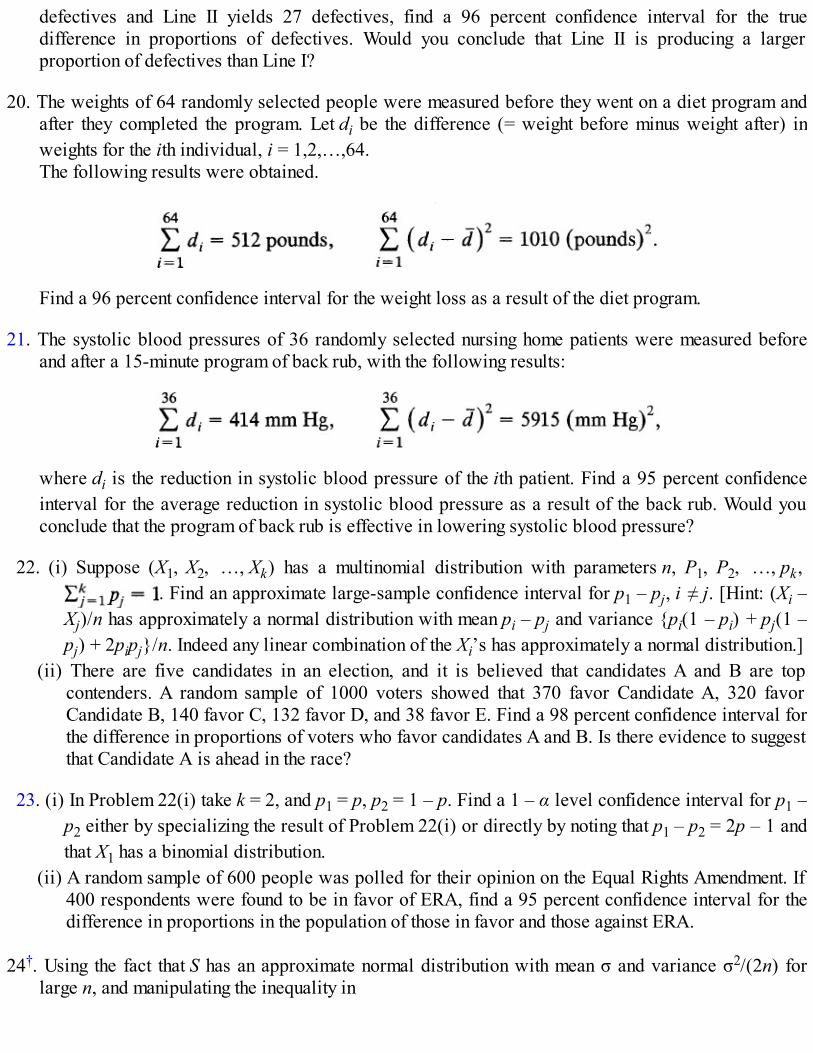
defectives and Line II yields 27 defectives, find a 96 percent confidence interval for the truedifference in proportions of defectives. Would you conclude that Line II is producing a largerproportion of defectives than Line I?

20. The weights of 64 randomly selected people were measured before they went on a diet program andafter they completed the program. Let di be the difference (= weight before minus weight after) inweights for the ith individual, i = 1,2,…,64.The following results were obtained.

Find a 96 percent confidence interval for the weight loss as a result of the diet program.

21. The systolic blood pressures of 36 randomly selected nursing home patients were measured beforeand after a 15-minute program of back rub, with the following results:

where di is the reduction in systolic blood pressure of the ith patient. Find a 95 percent confidenceinterval for the average reduction in systolic blood pressure as a result of the back rub. Would youconclude that the program of back rub is effective in lowering systolic blood pressure?

22. (i) Suppose (X1, X2, …, Xk) has a multinomial distribution with parameters n, P1, P2, …, pk, . Find an approximate large-sample confidence interval for p1 – pj, i ≠ j. [Hint: (Xi –

Xj)/n has approximately a normal distribution with mean pi – pj and variance {pi(1 – pi) + pj(1 –pj) + 2pipj}/n. Indeed any linear combination of the Xi’s has approximately a normal distribution.]

(ii) There are five candidates in an election, and it is believed that candidates A and B are topcontenders. A random sample of 1000 voters showed that 370 favor Candidate A, 320 favorCandidate B, 140 favor C, 132 favor D, and 38 favor E. Find a 98 percent confidence interval forthe difference in proportions of voters who favor candidates A and B. Is there evidence to suggestthat Candidate A is ahead in the race?

23. (i) In Problem 22(i) take k = 2, and p1 = p, p2 = 1 – p. Find a 1 – α level confidence interval for p1 –p2 either by specializing the result of Problem 22(i) or directly by noting that p1 – p2 = 2p – 1 andthat X1 has a binomial distribution.

(ii) A random sample of 600 people was polled for their opinion on the Equal Rights Amendment. If400 respondents were found to be in favor of ERA, find a 95 percent confidence interval for thedifference in proportions in the population of those in favor and those against ERA.

24†. Using the fact that S has an approximate normal distribution with mean σ and variance σ2/(2n) forlarge n, and manipulating the inequality in

show that

is also a 1 – α level confidence interval for σ.

25†. Let X1, X2, …, Xm and Y1, Y2, …, Yn be independent random samples from two populations withunknown variances and . Find a large sample confidence interval for σ1 – σ2 with approximateconfidence level 1 – α. {Hint: S1 – S2 has an asymptotic normal distribution with mean σ1 – σ2 andvariance [ /(2m) + /(2n)].}

26. Sample size for difference of means: Suppose X1, X2, …, Xn and Y1, Y2, …, Yn are independentrandom samples from two populations with means μ1, μ2 and variances , respectively. Showthat the sample size required in order to estimate μ1 – μ2 by – to within ε of μ1 – μ2 with 1 – αlevel confidence is given by

27. Sample size for difference of proportions: Let 1, 2 be two sample proportions (both based onsamples of the same size n) from populations with proportions p1 and p2 respectively. Suppose 1, 2 are independent. Show that the smallest n required in order that

is given by

If no prior knowledge of p1 and p2 is available, then we choose

9.7 LARGE-SAMPLE HYPOTHESIS TESTING

In many problems the interest is not in the estimation of an unknown parameter θ but in checking thevalidity of a certain statement about θ. Do the coffee jars contain 10 ounces of coffee per jar as the labelclaims? Do the men and women students at a certain state university have the same grade point averages?This problem of hypothesis testing has been considered for small samples in Sections 6.5 and 8.7 forspecific distributions. We now consider the case when the sample size is large.

Let = (X1, X2, …, Xn) be a point estimate of θ based on a random sample X1, X2, …, Xn. Suppose

has an asymptotic normal distribution with mean θ and variance . This fact can be used to testhypotheses such as H0: θ = θO against one-sided or two-sided alternatives. Under H0, the statistic

has approximately a standard normal distribution for sufficiently large n. By (θ0) in the denominator,we mean the standard deviation of computed under the assumption that θ = θO. Thus if = , θ0 = μ0,then (θ0) = σ/ irrespective of what θ0 is. However, if = , θ0 = p0, then (θ0) =

and we do not need to use in computing z. Similarly, if θ = p1

– p2, = 1 – 2 and θ0 = 0, then under H0: p1 = p2 = p (unknown) so that

Since p is unknown, however, we estimate it by

where X and Y are the respective number of “successes” in the first and second samples. Then

and

is the appropriate test statistic.If θ = σ, then = S and† = σ/ and under H0 : σ = σ0, (σ0) = σ0/ so that the appropriate

test statistic is

Clearly, large values of support θ > θ0 so that large values of Z tend to discredit H0: θ = θ0 againstH1: 0θ > θ0. Similar arguments apply in the remaining cases.

Table 1 of Section 9.6 gives some common point estimates and their (estimated) asymptotic variances.How large should the sample size be in order to apply this procedure? This question has been

answered in Remark 9.6.1. See also Remark 1 and Problems 19 and 20 in the section.

Example 1. Net Weight of Beer in a Can. A new filling machine has been put in use to fill 12-ounce beer cans. In order to check ifthe machine is operating properly, a random sample of 49 beer cans is taken. The cans are found to contain an average of 11. 89 ouncesof beer with a standard deviation of .36 ounce. Is the difference between the stated average and the observed average due to randomvariation? Here the null hypothesis of interest is H0: μ = 12 ounces to be tested against H1: 12. The observed value of the test statistics is

Under H0,

Thus in random sampling, if the process were operating according to specifications, there is only about a 3.24 percent chance of obtainingsuch an extreme value of sample mean weight. Hence, at significance level α ≥ .0324 we conclude that the difference in the sample meanweight and stated population mean weight is not due to chance fluctuation.

When testing for the proportion p, the appropriate test statistic is

where X, the number of successes, is integer valued. It would be wise to apply the continuity correction toimprove normal approximation. In the following example it does not much matter whether or not thecontinuity correction is applied. It is given here to illustrate the procedure and an alternative analysis ofthe Salk vaccine data of Example 9.4.5.

Example 2. Salk Vaccine Field Trial. In Example 9.4.5 we considered the following data from Salk polio vaccine field trial of 1954.

We applied an approximation to the Fisher–Irwin test of Section 6.4 to test the null hypothesis that the treatment has no effect. That is,under H0 the proportions of children who contracted polio is the same in the treatment as well as the control group.

There is yet another way to look at the data. There were about 402,000 children involved in the experiment. Each child had equalchance of being assigned to a treatment (vaccinated) or control (placebo) group. In all there were 148 cases of polio. Assuming that theassignment to the two groups had no effect on the outcome, could not the difference between 33 cases of polio in the treatment group and115 in the control group be due to random variation?

Here n = 148, H0: p = 1/2, H1: p ≠ 1/2, = 33/148 = .22. Rather than use

we note that X, the number of polio cases in the treatment group is 33 and the corresponding P-value is P(X ≤ 33). Since the critical regionis in the left tail

and

The associated P-value P(X ≤ –6.66) being less than 1 in 100 million, we have to conclude that the difference cannot be explained bychance variation. The only reasonable explanation is that the vaccine is effective. This is the same conclusion we arrived at in Example9.4.5.

Remark 1. (Sample Size Determination). Suppose σ is known and we wish to find the smallestsample size required to test H0: μ ≤ μ0 against H1: μ > μ0 such that the level is approximately a and theprobability of a type II error at some specified alternative μ(> μ0) is β. (Here μ is the population mean.)Then θ = μ, = and we reject H0 at level α if

We need to choose n such that

It follows that

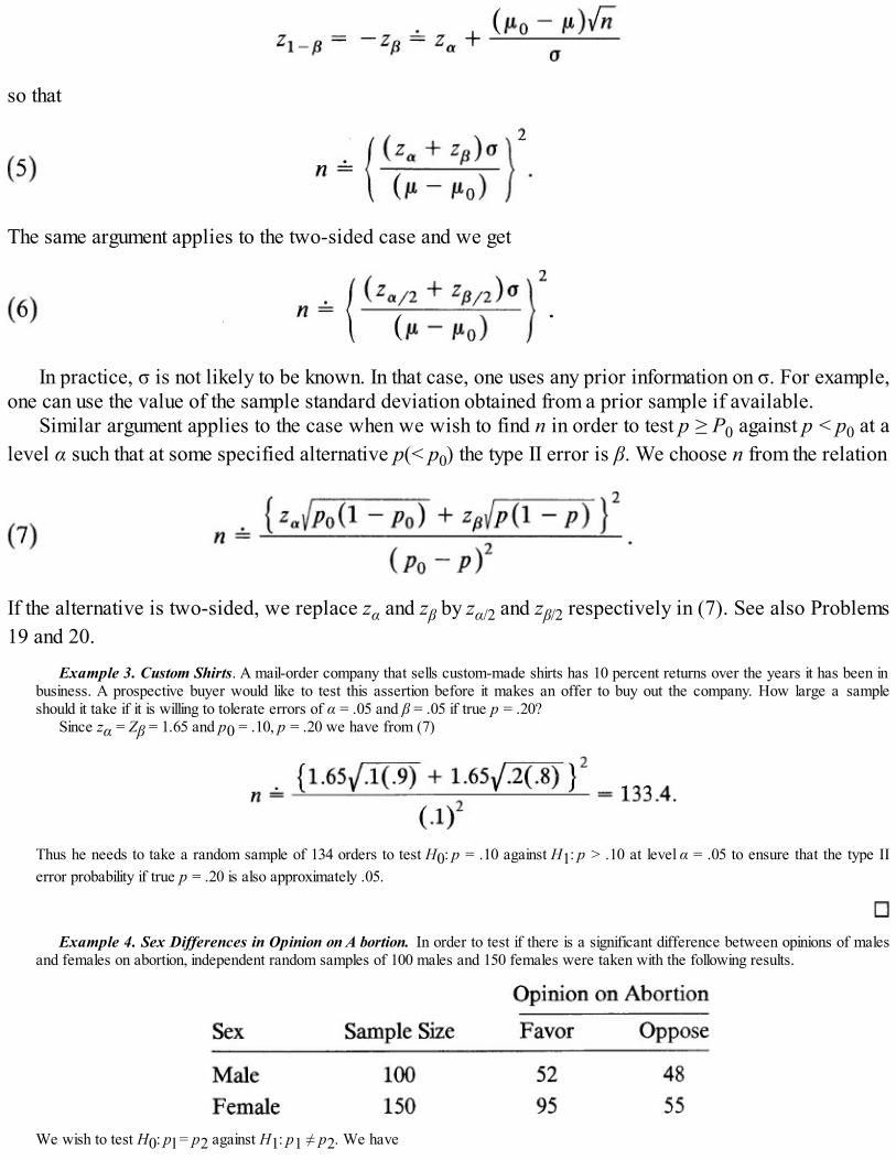
so that

The same argument applies to the two-sided case and we get

In practice, σ is not likely to be known. In that case, one uses any prior information on σ. For example,one can use the value of the sample standard deviation obtained from a prior sample if available.

Similar argument applies to the case when we wish to find n in order to test p ≥ P0 against p < p0 at alevel α such that at some specified alternative p(< p0) the type II error is β. We choose n from the relation

If the alternative is two-sided, we replace zα and zβ by zα/2 and zβ/2 respectively in (7). See also Problems19 and 20.

Example 3. Custom Shirts. A mail-order company that sells custom-made shirts has 10 percent returns over the years it has been inbusiness. A prospective buyer would like to test this assertion before it makes an offer to buy out the company. How large a sampleshould it take if it is willing to tolerate errors of α = .05 and β = .05 if true p = .20?

Since zα = Zβ = 1.65 and p0 = .10, p = .20 we have from (7)

Thus he needs to take a random sample of 134 orders to test H0: p = .10 against H1: p > .10 at level α = .05 to ensure that the type IIerror probability if true p = .20 is also approximately .05.

Example 4. Sex Differences in Opinion on A bortion. In order to test if there is a significant difference between opinions of malesand females on abortion, independent random samples of 100 males and 150 females were taken with the following results.

We wish to test H0: pl = p2 against H1: p1 ≠ p2. We have

Hence

The corresponding P-value is given by

Thus the observed difference between male and female respondents could very well be due to chance variation.

Example 5. Mean Ages of Females Using IUD’s. It is suspected that the average age of females who retain interuterine devicesas contraceptives is higher than those who expel the devices. Independent random samples of females who had retained IUD’s and thosewho had expelled IUD’s were taken with the following results.

We wish to test H0: μ1 < μ2 = 0 against the alternative H1: μ1, < μ2. We have

with associated P-value

Thus under H0 there is only 1.6 percent chance of obtaining such an extreme value of z, and we have to conclude that the difference inages is significant at levels α ≥ .0162. That is, we reject H0 and conclude that the mean age of females who retain the IUD’s is higherthan those who expel it.

Remark 2. If the level of significance α is preassigned, then the methods of Section 9.6 and 9.7 areessentially the same. The difference lies in the objective. The objective of a test is to reach a decisionwhether or not to reject a null hypothesis. The confidence interval, on the other hand, gives a range ofpossible values for the unknown parameter. The objective is to state, with a high degree of confidence, aninterval for the true value of the unknown parameter.

Remark 3. In view of Remark 9.6.2 we can test hypotheses concerning the mean of a finite population(or the difference between means) in sampling without replacement. The appropriate test statistic fortesting μ = μ0 is

where S is the sample variance, N is the size of the population and n is the sample size.

Problems for Section 9.7

In each problem, state clearly the null and alternative hypotheses, compute the P-value, and state yourconclusion.

1. The average mortality rate for a certain disease is 24 out of 100 attacks. A new treatment for thedisease is tested on 300 patients. There were 54 deaths. What can you say about the efficacy of thistreatment?

2. A random sample of 400 registered voters showed that if the election were held on the day the pollwas taken 216 of the respondents will vote for Candidate A. Does Candidate A have any reason foroptimism?

3. A filling machine is set up to fill cans with orange juice with an average of 48.05 ounces. Thestandard deviation in fill is set at σ = .20 ounce. A random sample of 36 filled cans from this machineis taken and it is found that the sample mean is 47.82 ounces with a standard deviation of .28 ounce.

(i) Is the sample standard deviation of .28 ounce consistent with the setting of σ = .20 ounce?(ii) Is the sample mean of 47.82 ounces consistent with the setting of μ = 48.05 ounces?

4. A branch manager of a bank will hire a new teller if the average service time of customers is morethan 4 minutes. She takes a random sample of 50 customers and finds that the sample mean is 4.5minutes with a standard deviation of 1.5 minutes. Should she hire a new teller?

5. A circuit fuse is designed to bum out as the current reaches 15 amperes. A random sample of 49 fusesis selected from a large lot and each fuse is tested for its breaking point. The following results areobtained:

Does the lot confirm to the specification?

6. The average miles per gallon (mpg) of lead-free gasoline for a new model is claimed to be 42. Anindependent consumer protection group, believing that the claim is exaggerated, tests 40 cars of thisparticular model and finds that the sample mean is 40.8 mpg with a standard deviation of 4.2 mpg. Atwhat level should the agency reject the manufacturer’s claim?

7. A leading manufacturer of dishwashers claims that 90 percent of its dishwashers do not require anyrepairs for the first four years of operation. A random sample of 164 dishwashers showed that 28dishwashers required some repair during the first four years of operation. Is there evidence to doubtthe manufacturer’s claim?

8. The advertisements for a gasoline additive claim that it results in an increase in mileage. In order to

check this claim a certain car model is selected with an average mpg of 18.7. A random sample of 49runs with the additive showed a sample mean of 19.6 mpg with a standard deviation of 3.6 mpg. Isthere evidence to support the advertised claim?

9. A new filtering device is under consideration in a chemical plant. Prior to installation of the newdevice a random sample of size 32 yields an average of 11.2 percent impurity with a standarddeviation of 8.6 percent. After the device was installed a random sample of size 42 yielded anaverage of 9.4 percent impurity with a standard deviation of 8.1 percent. Is the reduction in impuritysignificant? At what level?

10. Two machines fill milk in one-pint cartons. Independent random samples from the two machinesproduced the following results on net fill weights.

Is the difference in sample averages significant? At what level?

11. Independent random samples of fraternity and nonfraternity students at a state university yielded thefollowing grade point averages:

Is there evidence to suggest that the mean GPA of fraternity and nonfratemity students are different?

12. In an attempt to verify the claim that the absentee rate in Friday morning classes is higher than that inMonday to Thursday morning classes, independent random samples of students were taken. Theyyielded the following results.

Do the data support the claim?

13. Suppose that patients suffering from headaches are randomly assigned to one of two treatments. In thefirst treatment patients are given a placebo while in the second treatment patients are given a painreliever. After four hours it is found that 10 out 36 patients in the first group and 20 out of 42 patientsin the second group report no headache. At what level is the difference between the two proportions

significant?

14. Independent random samples of voters are taken in the South and in the North, and they are asked ifthey favor a bill to ban handguns. The following results are obtained.

What conclusion do you draw from this data?

15. A study is conducted to see if the average length of stay in a hospital of insured patients is more thanthat of uninsured patients. The following results are obtained.

Do the data support the belief that the average length of stay in a hospital of insured patients is morethan that of uninsured patients?

16. (i) Le t X1, X2, …, Xm and Y1, Y2, …, Yn be independent random samples from populationdistributions with respective means μ1 and μ2, and variances and . How will you test H0: σ1= σ2 against the usual one-sided or two-sided alternatives in the case when m and n are large?

(ii) Apply the result in (i) to test H0: σ1 = σ2 against H1: σ1 ≠ σ2 for the data in Problem 15.(iii) For the data of Problem 10, is there evidence to suggest that the fill variance for machine 1 is

less than that for the machine 2?

17. Suppose it is required to test H0: μ = 5 against H1: μ > 5 at level α = .05 such that the probability oftype II error when true μ = 6 is β = .05. What should be the minimum sample size if a isapproximately 3.5?

18. How many tosses of a coin should be made in order to test H0: p = 1/2 (coin fair) against H1: p > 1/2(loaded in favor of heads) at level α = .05 such that if the true p is .6 then β, the probability of type IIerror is .1?

19. (i) Find the minimum sample sizes required in order to test H0: μ1 – μ2 = 0 against H1 : μ1 ≠ μ2 atlevel α such that the probability of type II error at (μ1, μ2)μ1 ≠ μ2 is approximately β. Assume thatindependent samples of the same size are to be taken. Also find an expression for the commonsample size in the case of one-sided alternatives. (Assume that the variances , are known.)

(ii) Find the common sample size n in order to test H0: μ1 = μ2 against μ1 > μ2 at level α = .01 suchthat β = .05 when μ1 – μ2 = 5.

(iii) Do the same for testing H0: μ1 = μ2 against H1: μ1 ≠ μ2 when α = .1 and β = .1 when μ1 – μ2 = 2.

20. (i) In order to test H0: p1 = p2 against p1 ≠ p2 at level α, independent random samples of sizes n andn are to be taken to ensure that the probability of type II error at specified alternatives (p1, p2), p1≠ p2, is approximately β. Show that the minimum common sample size required is given by

where qi = 1 – pi, i = 1,2. Find the minimum sample size when the alternative is one-sided.(ii) For the Salk vaccine field trial (Example 2), find the common sample size required for testing H0:

p1 = p2 against H1: p1 > p2 (p1 = probability of a child from the control group getting polio, p2 =probability of a child from the treatment group getting polio) with α = .05 and β = .15 when p1 =.0001 and p2 = .00005.

(iii) Suppose H0: p1 = p2 is to be tested against H1: p1 ≠ p2. Find the common sample size n if α = .01and β = .05 when p1 = .5 and p2 = .6.

21. Modify the Fisher-Irwin test of Section 6.4 for testing p1 = p2 against p1 < p2 (or p1 > p2) when thesample sizes m and n are large.

9.8 INFERENCE CONCERNING QUANTILES

Consider a random sample X1 …, Xn from a continuous distribution function F ∈ Nothing else isknown about . Then is a nonparametric family. Let X(1) 4 X(2) < … < X(n) be the sample orderstatistic. In Section 8.5 we considered the problem of estimating the quantile of order p of F by thecorresponding sample quantile. We now consider some large sample properties of sample quantiles asestimates of population quantiles.

Assume that the quantile of order p, ζp is uniquely determined by

Let be the sample quantile of order p defined by

where [x] is the integral part of np.The following result is useful in statistical inference concerning quantiles. The proof is beyond our

scope and is omitted.

THEOREM 1. Let X(r) be the rth order statistic in sampling from a continuous distribution withdensity f. Then, as n → ∞ such that r/n → p (fixed), the distribution of

tends to that of the standard normal distribution, where μ satisfies F(μ) = p for p = r/n.According to Theorem 1, for large n, the sample order statistic is approximately normally

distributed with mean ζp , and variance p(1 – p)/(n[f(ζp)]2). In particular, is a consistent estimate of ζp.Theorem 1, however, is practically useless for constructing confidence intervals for ζp (unless, of

course, f is known). The case of most interest is when f is not known. In that case we use normalapproximation to binomial distribution.

From (8.5.15) we recall that for any distribution function, discrete or continuous,

so that [X(r), X(s)] is a confidence interval for ζp at level ≥ 1 – α if we choose r and s such that?

Let Y have a binomial distribution with parameters n and p. Then (2) can be rewritten as

and using normal approximation with continuity correction we have, for large n,

where Z has a standard normal distribution. We choose r and s by assigning equal probability to each tail.In that case

However, r and s need not be integers as required. So we choose r to be the largest integer and s to be the smallest integer ≥ np + 1/2 + .

In the special case when p = 1/2 and ζ.5 is the median, then an approximate 1 – α level confidence intervalfor large n is [X(r), X(n–r+1)] where r is the largest integer less than or equal to

Large Sample Equal Tails Confidence Interval for ζp

An approximate 1 – α level confidence interval for ζp for large n is given by [X(r), X(s)] where ris the largest integer ≤ np + 1/2 – and s is the smallest integer ≥ np + 1/2 +

.

We emphasize that since (l)–(3) are valid for any distribution, discrete or continuous, the above largesample confidence interval is also valid for any distribution.

Example 1. Median Family Income. A random sample of 36 family incomes in suburban Detroit yielded the following incomes (inthousands of dollars per year):

Suppose we wish to estimate the median family income for this suburb by a 95 percent confidence interval. Since α = .05, zα/2 = 1.96, and

so that r = 12 and s = 25. Thus an approximate 95 percent confidence interval is given by

Ordering the incomes in increasing order, we get

so that x(12) = 34 and x(25) = 50 and the 95 percent confidence interval for median income is 34 ≤ ζ.5 ≤ 50 (in thousands of dollars).If we want a 90 percent confidence interval for the .75 quantile, then zα/2 = 1.645, np = 36(.75) = 27 and

It follows that r = 23 and s = 32 and the 90 percent confidence interval is 49 ≤ ζ.75 ≤ 82, in thousands of dollars.

Example 2. Sample Quantile as Estimate of Population Quantile. Suppose a sample of size 100 is taken from a normal populationwith mean μ and variance 1. What is the probability of observing a sample quantile of order .75 larger than .25?

We note that ζ.75 is given by

where X is normal with mean μ and variance 1. Hence

so that ζ.75 = μ + .67. Also

In view of Theorem 1, the sample quantile of order .75, that is, X(75), has approximately a normal distribution with mean ζ.75 and variance

Hence

where Z is a standard normal random variable. If, for example, μ = – .50, then ζ.75 = .17 and

In this case we can find a 1 – α level confidence interval for ζ.75 from Theorem 1. In view of the approximate normality of X(75), a 1– α level confidence interval is given by

We can also use Theorem 1 to see how the nonparametric estimate X(75) of ζ.75 performs compared with the parametric estimate.Because ζ.75 = .67 + μ, a good estimate (consistent, unbiased) of ζ.75 is given by

with MSE( = variance) given by

According to Theorem 1, however,

so that the relative efficiency of .75 with respect to X(75) is given by

This means that we are losing about half the sample size by using X(75) instead of .75. However, what we lose in terms of sample sizeis balanced by the assurance that X(75) is a good estimate of ζ.75 even if the underlying distribution is not normal (as long as it iscontinuous and has a unique quantile of order .75).

Remark 1. How large should n be in order to apply results of this section? In general, we are guidedby Table 1 of Section 9.4. As long as np(1 – p) 5 10, the approximation is quite good. For p = 1/2approximation is fairly good for n 5 20. For values of p near zero or 1, one should check to see if n islarge enough that np(1 – p) 5 10. For intermediate values of p we will use the approximation even forvalues of n as small as 30 but it should be understood that the approximation may not be that good.

Remark 2. As pointed out in Section 8.5, given α and n there may not exist a confidence interval [Xr,X(s)] for ζp at level 1 – α. According to Problem 8.5.28, such is the case when α < pn + (1 – p)n. Thus,for n = 40, α = .01 there does not exist a confidence interval of the form [X(r), X(s)] for ζ.1. In such cases,either the value of r selected according to (5) will be necessarily less than 1 or the value of s selectedaccording to (5) will be greater than n. If, however, α ≥ pn + (1 – p)n and s selected according to (5) is >n, then one should find the largest r such that [X(r), X(n)] is a 1 – α level confidence interval for ζp.Similarly, if α ≥ pn + (1 – p)n and r selected according to (5) is < 1, then one chooses the smallest s suchthat [X(r), X(n)] is a 1 – α level confidence interval for ζp. Thus for α = .01, n = 60 and p = .9, α = .01 ≥ pn

+ (1 – p)n = .002, but s according to (5) is 61. Hence we find the largest r such that [X(r), X(60)] includesζ.9. We have

where Y is binomial with n = 60 and p = .9. Applying normal approximation, we choose the largest r suchthat

or such that

Thus

so that

and we choose r = 48. The level of [X(48), X(60)] is in fact .9915.

Remark 3. If α < pn + (1 – p)n so that no confidence interval [X(r), X(s)] at level 1 – α exists, then wehave two choices: either take a larger sample size (such that α ≥ pn + (1 – p)n) or increase α and hencedecrease the confidence level.

Remark 4. Testing Hypotheses Concerning Quantiles. In Section 8.5.2 we saw that hypothesesconcerning ζp of the form ζp = ζ0 against one-sided or two-sided alternatives can be tested by using a signtest based on binomial distribution. If n is large (see Remark 1) we can use normal approximation ofTheorem 1 if f is known and normal approximation to binomial if f is unknown. Since tests based on Z, astandard normal random variable, have been described in detail in Section 8.7.3, we omit these details.Similar remarks also apply to the median and the Fisher–Irwin tests of Section 6.4.

Problems for Section 9.8

1. The birth weights (in pounds) of 40 infants at a county hospital are found to be:

(i) Find an approximate 100(1 – α) percent confidence interval for the median birth weight if (a) α =.10; (b) α = .01.

(ii) Find an approximate 95 percent confidence interval for the quantile of order .6.

2. The ages of patients in a coronary care unit of a hospital were recorded for a sample of 49 patients asfollows.

Find an approximate 100(1 – α) percent confidence interval for the median and the quantile of order.25 for the age distribution of coronary patients when:(i) α = .02.(ii) α = .05.

3. A random sample of 50 ranches in western Texas gave the following acreages:

Find an approximate 100(1 – α) percent confidence interval for the median acreage of a ranch inwestern Texas if (a) α = .05, (b) α = .10.

4. The lifetimes of 121 light bulbs manufactured by a certain company shows a sample median of 1207hours. The lifetimes may be assumed to have an exponential distribution.(i) Use Theorem 1 to find the probability that the sample median is less than 1207 hours. (Take the

population mean to be 1250 hours.)(ii) Find a 95 percent confidence interval for the median lifetime of bulbs made by this company.(iii) Compare the relative efficiency of the parametric estimate In 2 of the median with the

nonparametric estimate of the median. (Here μ, is the mean lifetime of the exponentialdistribution.)

5. Suppose a sample of 75 observations is taken from the distribution

Find the probability that the sample quantile of order .2 will be larger than .60.

6. A large company uses small foreign-made cars for its sales force. A random sample of 48 repair billsyielded the following results (in dollars):

Find an approximate 90 percent confidence interval for the median repair bill for this company’s fleetof cars.

7. Suppose X1, X2, …, Xn is a random sample from density function f(x|θ) as given below. An estimate ofthe median of f is desired. Compute the relative efficiency of the parametric estimate (choose the bestunbiased estimate) relative to the sample median.(i) .(ii) f(x|θ) = 1/θ, 0 4 x < θ, and zero elsewhere (see Example 8.5.4).

In each case find a 1 – α level confidence interval for the median based on the sample median.

8. A random sample of 40 observations is taken from a uniform distribution on [0, θ] with the followingresults:

(i) Construct a 95 percent confidence interval for the median by ignoring the fact that the samplecomes from a uniform distribution.

(ii) Construct a 95 percent confidence interval for the median using the fact that the sample comesfrom a uniform distribution on [0, θ].

9. For the data of Problem 1 test the hypothesis that the median birth weight is less than or equal to 7.3pounds at a 5 percent level of significance.

10. For the data on ages of patients in coronary care (Problem 2), test the hypothesis that the quantile oforder .25 is 38 years against the two-sided alternative.

11. The diastolic blood pressures of 38 randomly selected men were found to be:

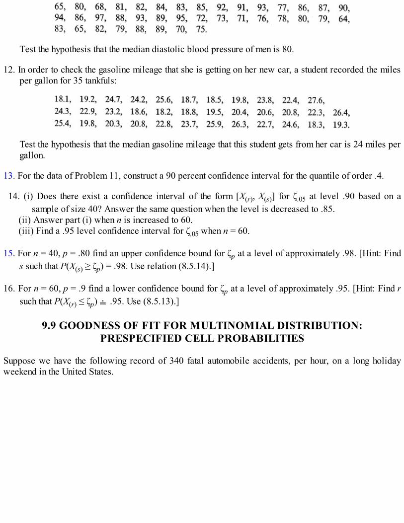
Test the hypothesis that the median diastolic blood pressure of men is 80.

12. In order to check the gasoline mileage that she is getting on her new car, a student recorded the milesper gallon for 35 tankfuls:

Test the hypothesis that the median gasoline mileage that this student gets from her car is 24 miles pergallon.

13. For the data of Problem 11, construct a 90 percent confidence interval for the quantile of order .4.

14. (i) Does there exist a confidence interval of the form [X(r), X(s)] for ζ.05 at level .90 based on asample of size 40? Answer the same question when the level is decreased to .85.

(ii) Answer part (i) when n is increased to 60.(iii) Find a .95 level confidence interval for ζ.05 when n = 60.

15. For n = 40, p = .80 find an upper confidence bound for ζp at a level of approximately .98. [Hint: Finds such that P(X(s) ≥ ζp) = .98. Use relation (8.5.14).]

16. For n = 60, p = .9 find a lower confidence bound for ζp at a level of approximately .95. [Hint: Find rsuch that P(X(r) ≤ ζp) .95. Use (8.5.13).]

9.9 GOODNESS OF FIT FOR MULTINOMIAL DISTRIBUTION:PRESPECIFIED CELL PROBABILITIES

Suppose we have the following record of 340 fatal automobile accidents, per hour, on a long holidayweekend in the United States.

The number X of fatal auto accidents per hour is clearly a discrete random variable. We should like toknow the distribution of X. In Section 4.5 we studied some graphical methods of looking at the data todetermine if the data could have come from one of a particular family of distributions. One method thatwe had suggested was to draw a graph of the relative frequency histogram and check visually to see if thehistogram looks much like the histogram of one of the known discrete distributions (studied in Chapter 6).We did not, however, provide an overall measure of the goodness of fit. How well does an assumeddistribution fit the histogram data? For example, suppose we feel that the Poisson distribution with λ = 5provides an adequate representation for the distribution of X. We can now draw the (observed) relativefrequency histogram and the postulated (or expected) relative frequency histogram on the same graph tosee how close the agreement is. The following table compares the observed and the postulated relativefrequencies: (See Example 1 below for details of computations.)

In Figure 1 below we have plotted the two relative frequency histograms.The two histograms appear close. The question we have to answer, however, is the following: Is the

difference between the two histograms due to chance fluctuation, or is there something wrong with ourassumption about the model? We now study the chi-square test of goodness of fit which is speciallydesigned to answer this question.

Consider a random sample X1, X2, …, Xn from a discrete distribution given by

where pj < 0 and . How do we use the observations to test the null hypothesis

Figure 1. Relative frequency histograms. The open-ended class 8 or more is not included.

where pj0 are known numbers? Let

Then nj, j = 1,2,…,k, are random variables such that and, more over, (n1, n2, …, nk–1) has,under H0, a multinomial distribution with parameters . since each nj has a marginalbinomial distribution with parameter pj, we have

and we can use nj/n,j = 1,2, …, k respectively as estimates of p1, p2, …, pk. It is natural to compare theobserved proportions nj/n and the postulated proportions pj

0. It is tempting to use a distance function suchas

as a measure of the agreement between H0 and the observations. The smaller this distance the greater theagreement. The measure most commonly used in practice, however, is the weighted sum of squares.

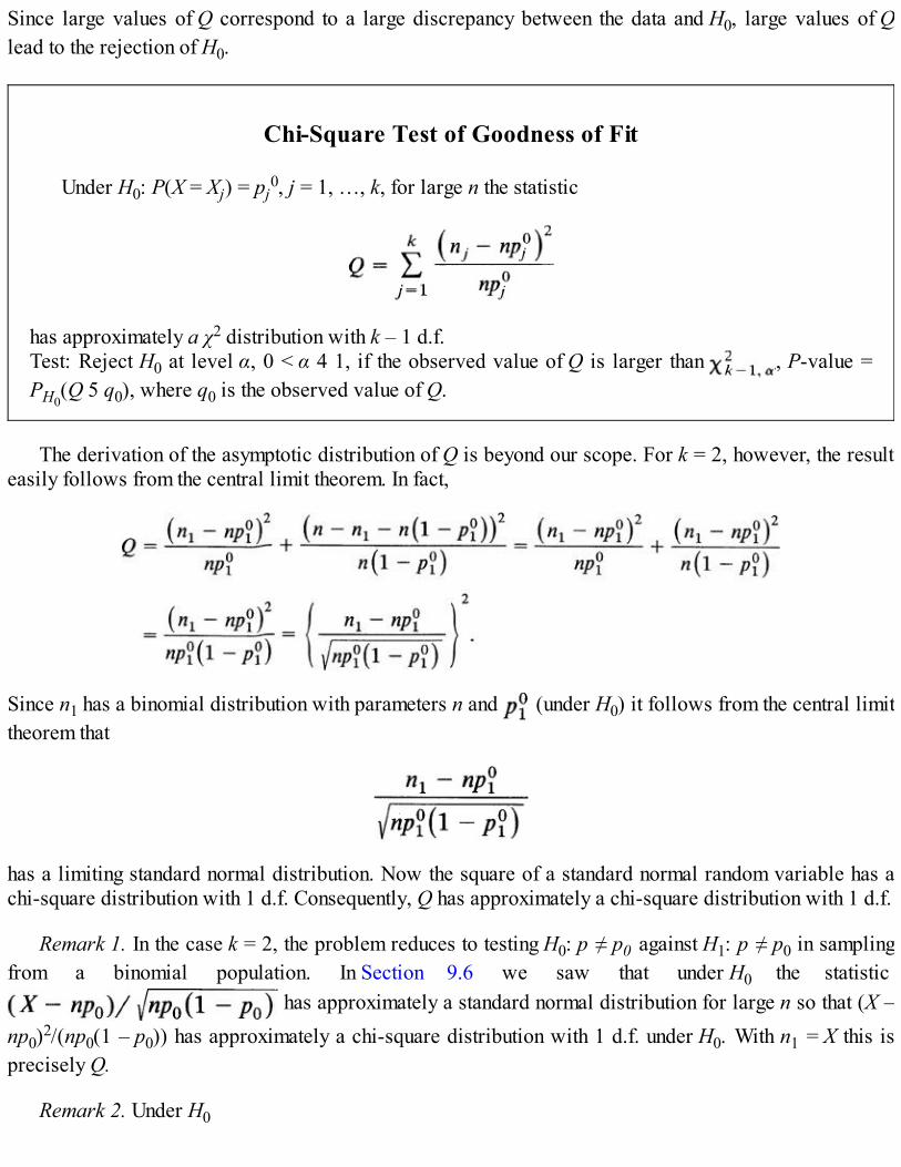
Since large values of Q correspond to a large discrepancy between the data and H0, large values of Qlead to the rejection of H0.

Chi-Square Test of Goodness of Fit

Under H0: P(X = Xj) = pj0, j = 1, …, k, for large n the statistic

has approximately a χ2 distribution with k – 1 d.f.Test: Reject H0 at level α, 0 < α 4 1, if the observed value of Q is larger than , P-value =PH0

(Q 5 q0), where q0 is the observed value of Q.

The derivation of the asymptotic distribution of Q is beyond our scope. For k = 2, however, the resulteasily follows from the central limit theorem. In fact,

Since n1 has a binomial distribution with parameters n and (under H0) it follows from the central limittheorem that

has a limiting standard normal distribution. Now the square of a standard normal random variable has achi-square distribution with 1 d.f. Consequently, Q has approximately a chi-square distribution with 1 d.f.

Remark 1. In the case k = 2, the problem reduces to testing H0: p ≠ p0 against H1: p ≠ p0 in samplingfrom a binomial population. In Section 9.6 we saw that under H0 the statistic

has approximately a standard normal distribution for large n so that (X –np0)2/(np0(1 – p0)) has approximately a chi-square distribution with 1 d.f. under H0. With n1 = X this isprecisely Q.

Remark 2. Under H0

How do we use Q to test that X has a specified probability density function f? The answer issurprisingly simple. Divide the real line into k intervals I1, …, Ik and let = Pf(X ∈ Ij), j = 1, …, k. Let

j be the observed proportion of observations that fall in the interval Ij Then the statistic

has approximately a chi-square distribution with (k – 1) d.f. under H0.How do we choose the intervals I1, I2, …, Ik? The first point to remember is that the chi-square

distribution is only an approximation to the true distribution? of Q. So the choice has to be made in such away that this approximation is good. The second point to remember is that the underlying assumption tothe chi-square approximation is that each random variable has approximately a

normal distribution (with mean 0 and variance 1 – ). This holds provided n is large. Suppose issmall for some cell. Then for the approximation to be good we would want either n to be very large or n

to be large. (Recall that if the mean λ → ∞ then the Poisson distribution can be approximated by thenormal distribution.) If n is small then the term (nj – n )2/n may dominate the other terms of Q dueto a small denominator. Although the approximation is often good even when n is as small as 1, thefollowing rules of thumb are often used in choosing I1, I2, …, Ik.

(i) Choose I1, I2, …, Ik such that under H0, = P(X ∈ Ij) is approximately equal to 1/k and each n n/k ≥ 5.

(ii) If any of the n ’s is less than 5, pool the corresponding interval with one or more intervals tomake the cell frequency at least 5. The decision which intervals (or cells) to pool is arbitrarybut we restrict pooling to a minimum. The degrees of freedom associated with the chi-squareapproximation, after pooling, are reduced by the number of classes pooled.

Example 1. Fatal Auto Accidents on a Long Weekend. We return to the data on fatal auto accidents given at the beginning of thissection. Suppose we wish to test the hypothesis H0 that the number of fatal auto accidents X, per hour, has a Poisson distribution withmean λ = 5. Under H0,

From Table A4 we have

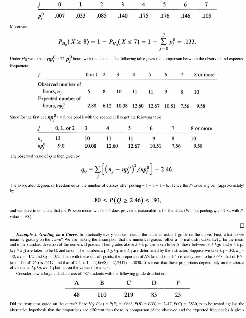
Moreover,

Under H0 we expect = 72 hours with j accidents. The following table gives the comparison between the observed and expectedfrequencies.

Since for the first cell > < 5, we pool it with the second cell to get the following table.

The observed value of Q is then given by

The associated degrees of freedom equal the number of classes after pooling – 1 = 7 – 1 = 6. Hence the P-value is given (approximately)by

and we have to conclude that the Poisson model with λ = 5 does provide a reasonable fit for the data. (Without pooling, q0 = 2.82 with P-value = .90.)

Example 2. Grading on a Curve. In practically every course I teach, the students ask if I grade on the curve. First, what do wemean by grading on the curve? We are making the assumption that the numerical grades follow a normal distribution. Let μ be the meanand σ the standard deviation of the numerical grades. Then grades above λ + k1σ are taken to be A, those between λ + k2σ and μ + k1σ,(k1 > k2) are taken to be B, and so on. The numbers k1, k2, k3, and k4 are determined by the instructor. Suppose we take k1 = 3/2, k2 =1/2, k3 = –1/2, and k4 = –3/2. Then with these cut-off points, the proportion of A’s (and also of F’s) is easily seen to be .0668, that of B’s(and also of D’s) is .2417, and that of C’s is 1 – 2(.0668) – 2(.2417) = .3830. It is clear that these proportions depend only on the choiceof constants k l, k2, k3, k4 but not on the values of μ and σ.

Consider now a large calculus class of 487 students with the following grade distribution:

Did the instructor grade on the curve? Here H0: P(A) = P(F) = .0668, P(B) = P(D) = .2417, P(C) = .3830, is to be tested against thealternative hypothesis that the proportions are different than these. A comparison of the observed and the expected frequencies is given

below:

The observed value of Q is given by

For 4 d.f. we note that under H0

and one can hardly argue that such a large value of q0 is due to chance variation. There is no agreement between the grades as given andgrades that would have been given had the instructor been grading on the curve (with 6.68 percent each of A’s and F’s, 24.17 percenteach of B’s and D’s and the rest C’s). ?

Example 3. Sampling from the Uniform Distribution (Example 4.5.4 Continued). In Example 4.5.4 a random sample of size 80was taken from the interval (0,1). In Table 4.5.2 we constructed the frequency distribution with 10 class intervals of equal width andcomputed the relative frequency histogram. After plotting the histogram and ogive estimates of the distribution along with the uniformdistribution (in Figures 4.5.6 and 4.5.7), we found that a visual comparison was inconclusive. Let us now test the null hypothesis H0, thatthe sample comes from the uniform distribution on (0,1). The following table gives the observed and expected frequencies.

We have

For 7 d.f. we note that

Hence the observed value of Q is not significant at 10 percent level and we cannot reject H0.

Remark 3. The procedure described here applies when the cell probabilities are completely

specified; that is, when H0 is a simple hypothesis. In many applications, however, this is not the case.Often the null hypothesis we wish to test is that the underlying distribution is normal or Poisson orgamma, and so on. The parameters are not specified and have to be estimated from the data. How do wemodify the test procedure when parameters are estimated? This is done in Section 11.7.

Remark 4. The chi-square test of goodness of fit tests H0: pj = , j = 1, 2,…, k against all possiblealternatives. In a specific problem we may be more interested in testing H0 against restricted alternativessuch as H1: pj < , j = 1, 2,…, k – 1 and pk > . A test specifically designed to test H0 against thisparticular H1 will usually perform better than the chi-square test in the sense that the chi-square test willbe more conservative. It is more difficult to reject H0 using the chi-square test at a given level α then itwould be if we were to use the test designed with the alternative H1 in mind. Nevertheless, the chi-squaretest should be used as a first test to decide whether the data can be regarded as a random sample from oneof a particular family of distributions. It should be used to answer questions such as: Do the data comefrom a normal distribution? Are the observations exponentially distributed?

Remark 5. We emphasize that the chi-square test is only a first step. If the test rejects a particular fit,we know that the postulated model is not a reasonable fit for the data. On the other hand, if the test acceptsa certain fit, it does not necessarily follow that the underlying distribution is the hypothesized distribution.Often the test will accept two or more dissimilar distributions. The test will accept as normal almost allunimodal symmetric distributions (see, for example, Problem 6). In such cases, further analysis of the datais necessary. (See, for example, Sections 4.4, 11.2, and 11.3.).

Remark 6. We know that sufficiently large values of Q lead to a rejection of H0 because these valuesof Q have small P-values. Very small values of Q should also be looked at with suspicion. Suppose, forexample, that a student is asked to roll a fair die 120 times and comes up with the following data.

Under H0 we expect each face value to appear 20 times, so the data produced by the student lookreasonable. In fact, they look too reasonable. We have

so that

Thus there is less than 1 chance in 100 that such a small value of Q could have come from actual tossingof a fair die 120 times. It is possible that the student did actually perform 120 tosses and came up withthese results but the data look suspicious. He may well have cooked up the data.

Problems for Section 9.9

1. An urn contains red, green, white, yellow, and blue marbles. In order to test the hypothesis

a random sample of 200 marbles is drawn from the urn with replacement. If the sample contains 25,15, 28, 45, 87 red, green, white, yellow, and blue marbles respectively, would you reject H0 at levelα = .10?

2. In order to test whether a particular coin is fair, the following procedure was designed. Fortysequences of four tosses each with the coin were observed and the number of heads recorded in eachsequence of four tosses as follows:

Would you accept the claim that the coin is fair?

3. The frequency distribution of 608 digits in the decimal expansion of π is as follows:

Is there sufficient evidence to conclude that each of the 10 digits 0, 1, …, 9 occurs with equalfrequency?

4. In a well known experiment, the geneticist Gregor Mendel crossbred yellow round peas with greenwrinkled peas. He observed the shape and color of a sample of 556 peas resulting from seeds of thiscrossbreeding with the following results:

(i) Round and yellow, 315. (ii) Round and green, 108.(iii) Wrinkled and yellow, 101. (iv) Wrinkled and green, 32.

According to Mendel’s theory, the corresponding frequencies should be in the ratio 9:3:3:1. Do thedata support his theory? Is the fit too good to be reasonable?

5. A student is asked to draw a random sample of 50 digits from a random number table. He comes upwith the following digits:

Test the hypothesis that these digits are random:(i) Count the frequency of each digit and test H0: pi = P(digit i) = 1/10, i = 0, 1, …, 9.(ii) Go through the list and count the number of times the next digit is the same as the preceding one

or one away (that is, next smaller or next larger) from the preceding one (assume 0 is one awayfrom 9). If the digits are random, p0 = P(next digit same) = 1/10 and p1 = P(next digit is oneaway) = 2/10. Test H0: p0 = 1/10, p1 = 2/10, p2 = P(neither) = 7/10, against all possiblealternatives. (See also Problem 14.)

6. A random sample of size 50 from a population produced the following data:

(i) Construct a frequency distribution with class intervals

(ii) Use the frequency distribution in part (i) to test if the data is normally distributed with mean 0and variance 1.

(iii) Could the data have come from the double exponential density function

(See also Example 11.2.3.)

7. The failure times of 100 transistor batteries of a certain kind in hours have the following frequencydistribution.

(i) Could the data have come from an exponential distribution with mean 50 hours?(ii) Could the data have come from an exponential distribution with mean 45 hours?

8. In order to test the hypothesis that a certain coin is fair, the coin is tossed until the first head shows up.The experiment is repeated 150 times with the following results:

Can we conclude that the coin is fair?

9. A computer program generates random numbers from the uniform distribution on [0,10). A sample of200 observations was found to have the following frequency distribution.

Is there strong evidence to conclude that the program is written properly?

10. The distribution of number of particles emitted from a radioactive source is thought to be Poissonwith mean λ = 2 per 10 second. In order to test this hypothesis, the number of particles emitted in 150consecutive 10-second intervals are recorded. They have the following frequency distribution:

How strong is the evidence against the claim?

11. The lifetime of a rotary motor is believed to have an exponential distribution with mean 2 years. Arandom sample of 80 motors was tested with the following results:

Is there sufficient evidence in support of the belief?

12. Show that

13. Suppose a die is rolled 120 times with the following results:

(i) Test the hypothesis that the die is fair.(ii) Test the hypothesis that the die is fair by pooling the frequencies for face values 1 and 2 and

those for face values 5 and 6.(iii) Test the same hypothesis by pooling the frequencies for the face values 1, 2, and 3 and those for

the face values 4, 5, and 6. (Now one can apply either the X2-test or the (equivalent) test forequality of two proportions.)

14. Suppose a student produces the following sample of 50 random digits:

(See Problem 5.)(i) Apply the test of Problem 5(i) to check if the digits are random.(ii) Apply the test of Problem 5(ii) to check if the digits are random.

9.10 REVIEW PROBLEMS

1. Use the continuity theorem (Theorem 9.2.1) to show that the weak law of large numbers holds insampling from the following distributions:

(i) f(x) = 1, 0 ≤ x ≤ 1, and zero elsewhere.(ii) f(x) = λ–1exp(–x/λ), x > 0, and zero elsewhere.

(iii) f(x) = (l/2)exp(–|x|), x ∈ .(iv) f(x) = 6x(l – x), 0 ≤ x ≤ 1, and zero elsewhere.

(See Problem 5.4.8.)

2. Show that

as n → ∞. [Hint: Use the central limit theorem on exponentially distributed random variables.]

3. If Xn has a chi-square distribution with n d.f., what is the limiting distribution of Xn/n2?

4*. Suppose X1, X2, … are independent random variables with probability function P(Xn = 1) = P(Xn = –

1) = 1/2 for all n = 1, 2, …. Let . Show that the limiting distribution of Zn is uniform

on [–1, 1].

5. Are the sufficient conditions for the Levy’s central limit theorem satisfied in random sampling fromthe following distributions?

(i)

(ii) f(x) = (l/2)exp(–|x|), x ∈ .

(iii)P(X = k)= , k = 1, 2, … where .

(iv) f(x) = (2x/β)exp( – x2/β), x > 0, and zero otherwise.

6. An urn contains eight identical marbles numbered 1 though 8. A random sample of n marbles is drawnwith replacement.

(i) What does the law of large numbers say about the appearance of the marble numbered 1 in ndraws?

(ii) How many drawings are needed to ensure that with probability at least .90 the relative frequencyof the occurrence of 1 will be between .12 and .13?

(iii) Use the central limit theorem to approximate the probability that among n numbers drawn thenumber 4 will appear between (n – )/8 and (n + )/8 (inclusive).

7. Ever watchful of the elections every two years, an Ohio state senator bases his decision on whether tovote for or against politically sensitive issues on the results of private polls. A bill to increase thestate income tax by 90 percent is before the Ohio Senate. The senator commissions a random sampleof 200 registered voters in his district. He will vote for the bill only if 100 or more voters are infavor. What is the probability that he will vote in favor of the bill if in fact only 40 percent of allvoters in his district are in favor of it? What is the probability that he will not vote for the bill if in

fact 55 percent of all voters in his district are in favor of it?

8. A random sample of 280 items is checked every hour from the production line of a certain machine. Ifthe number of defectives in the sample is six or less, then the machine is considered in control.Otherwise the machine is stopped. Find the probability of:

(i) Stopping the machine when it produces, on the average, 1.5 percent defective items.(ii) Not stopping the machine when it produces, on the average, 3 percent defective items.

9. From a very large shipment of 9-volt batteries, a random sample of 64 is checked. If the mean lengthof life of the sample is 75 hours or more the shipment is accepted; otherwise the shipment is rejected.

(i) Find the probability of accepting a shipment that has a mean life length of 72 hours with astandard deviation of 10 hours.

(ii) Find the probability of rejecting a shipment that has a mean life length of 80 hours with astandard deviation of 20 hours.

(iii) Find the probability of accepting (or rejecting) a shipment that has a mean life of 75 hours.

10. There are 150 female and 350 male faculty members at a junior state college. A random sample of 50faculty members is taken to fill 50 seats on the faculty senate. If the sample contains 12 female facultymembers, is there sufficient evidence for the female faculty members to complain aboutunderrepresentation?

11. In order to estimate the mean television viewing time (in hours) per American family per week, asocial scientist takes a random sample of 600 families and finds that the sample mean is 24.8 hourswith a standard deviation of 8.6 hours.

(i) Find a 96 percent confidence interval estimate of the mean weekly viewing time.(ii) If the social scientist wishes to estimate the mean time to within 1.5 hours with 95 percent

confidence, how large a sample should he take? Take a = 9 hours.

12. Let X1, X2, …, Xn be a random sample from a distribution function F. Let c be a known constant andsuppose θ(F) = θ = P(Xi > c) = 1 – F(c).

(i) Find a consistent estimate of θ.(ii) Find a consistent estimate of the odds ratio θ/(1 – θ).

13. Let Xl, X2, …, Xn be a random sample from a Poisson distribution. Find a consistent estimate of P(X =1).

14. Let X1, X2, … Xn be the lifetimes of n batteries of the same type. Suppose X1, X2, …, Xn areindependent and identically distributed with exponential distribution having mean θ. The estimate =nX(l) has certain advantages over the estimate . Is a consistent estimate of θ (Hint: See example8.5.2.)

15. Let (Xl, X2, …, Xk–1) have a multinomial distribution with parameters n, p1, p2, …, pk–1, pi > 0,

. Find a consistent estimate of pi – pj, i ≡ j. (See also Problem 9.6.22.)

16. Let (X1, Y1), (X2, Y2)…, (Xn, Yn) be a random sample from a bivariate distribution with

(i) What is the limiting distribution of – ?

(ii) Is – a consistent estimate of μ1 – μ2? Is it unbiased?

(iii) How will you test the null hypothesis H0: μ1 – μ2 = δ against the alternative hypothesis H1: μ1 –μ2 ≡ δ when σ1, σ2 are known and n is large? When σ1, σ2 are unknown and n is large?

17. Several studies have shown that twins have lower I.Q.’s in their early years than nontwins but theycatch up with the nontwins by about age 10. A psychologist believes that the slower intellectualgrowth of twins may be due to parental neglect. She takes a random sample of 49 sets of twins agedtwo years and finds that the mean attention time given to each pair of twins in a particular week is 28hours with a standard deviation of 10 hours.(i) Find a 92% confidence interval for the mean attention time given to all two-year-old twins.(ii) Suppose the national average mean attention time given two-year-old twins is 31 hours a week.

Is the observed mean time of 28 hours a week for families in the sample significantly lower thanthe national average?

18. An experiment is to be designed to test the mean lifetime of a particular component. The experimenteris willing to take a chance of 1 in 100 of rejecting a true H0: μ ≤ μ0, where μ is the mean lifetime. Ifthe true mean, however, is μ = μ1 (> μ0), the experimenter is willing to allow a chance of 5 in 100 ofaccepting H0: μ ≤ μ0. How large should the sample size n be if the test statistic used is , the samplemean? Assume that the population standard deviation is σ hours. In particular, find n when μ1 – μ0 = 5hours and σ = 10 hours.

19. The location of display of an item is important to the distributor. B. G. Vending Company has theoption of putting soft drink vending machines in either (or both) of two different locations. Thecompany decides to put one machine each in the two locations for a trial period of six weeks. Thenumber of cans sold each day from each machine is recorded with the following results.

(i) Is the difference between the mean number of cans sold per day in the two locations significant?(ii) Find a 90 percent confidence interval for the true difference in means.

20. The mean shelf-life (in days) of various products in a supermarket is important to the manager.Independent random samples of 64 cans of peaches of Brand A and Brand B are tested with thefollowing results.

(i) Is there sufficient evidence to conclude that the mean shelf-lives of the two brands are different?(ii) Find a 96 percent confidence interval for the true mean difference in shelf-lives of the two

brands.

21. Independent random samples of 100 cars in Washington, D. C., and 150 cars in Cleveland wereinspected for five specific safety-related defects. An inspected car is considered unsafe if it does notpass at least one of the five tests. The following results were obtained.

(i) Find a 90 percent confidence interval for the difference between the true proportions of unsafecars in Washington, D.C. and Cleveland.

(ii) Is there sufficient evidence to conclude that the proportion of unsafe cars in Cleveland is largerthan that in Washington, D. C.? (There is no mandatory city or state yearly inspection of cars inCleveland. In Washington, D.C., every registered car is inspected for safety every year.)

22. Suppose a major automobile company wishes to allow enough headroom in its automobiles toaccommodate all but the tallest 10 percent of the drivers. Previous studies show that the quantile oforder .90 was 68.2 inches. In order to validate the results of the previous studies a random sample of65 drivers is selected and it is found that the tallest 21 persons in the sample have the followingheights: 68.1, 70.4, 72.6, 73.1, 70.2, 68.5, 68.0, 68.2, 69.4, 67.6, 69.8, 70.1, 70.2, 75.8, 72.3, 71.8,69.1, 67.9, 68.4, 71.6, 74.2.(i) Find a 99 percent confidence interval estimate for the quantile of order .90 if it exists.(ii) Find a 90 percent confidence interval estimate for ζ9 if it exists.(iii) Is it reasonable to use ζ9 = 68.2 inches?

23. The lengths of life in hours of 36 Brand X 9-volt batteries were recorded as follows:

(i) Find a 96 percent confidence interval for ζ5.(ii) Is it reasonable to use 31.2 hours as the median life length of the batteries? [The sample was

generated from a table of random numbers from the uniform distribution on (0,1) by using thetransformation X = 45 , where Y is uniform on (0, 1). Thus the sample comes from an

exponential distribution with mean 45 and median 45 In 2 = 31.2.]

(iii) Test H0: ζ.5 = 31.2 against H1: ζ5 ≠ 31.2 when it is known that X has an exponential distributionso that under H0, the mean of X is 45 hours. [The statistic X(18) in view of Theorem 9.8.1 has anormal distribution, under H0, with mean 31.2 and variance p(1 – p)/n[f(31.2)]2.]

24. Let (Xl, Y1), (X2, Y2),…, (Xn, Yn)… be independent and identically distributed with , and ρ = ρ(Xi,

Yi). Show that is a consistent estimate of ρσ1σ2 and R =

S11/(S1S2) is a consistent estimate of ρ under appropriate moment conditions. (See also Example5.3.6.) Here S1, S2 are the sample standard diviations.

† Since Sn is a random variable, we mean P(Sn → ∞ as n → ∞) = 1.‡ For the general case when μ ≠ 0, σ ≠ = 1 define Yi = (Xi – μ)/σ, i = 1,2,…,n. Then Yi = 0 and var(Yi) = 1.* This section deals with a special topic. For most readers it will be sufficient to learn only the continuity correction given in (7) or (8).† In Problems 24 and 25 we have assumed that the sample comes from a nearly normal population† In Problems 24 and 25 we have assumed that the sample comes from a nearly normal population†Here we have assumed that the sample comes from a nearly normal population.

CHAPTER 10

General Methods of Point and Interval Estimation

10.1 INTRODUCTION

The problem of statistical estimation was first introduced in Section 4.3 where, for most part, weconsidered samples of size 1 or 2. This was mainly due to technical difficulties. We did not have enoughtools in hand to evaluate the worth of point estimates or to compute the numerical values of the confidenceinterval estimates. Nevertheless, we were able to consider several special cases in Chapters 5 to 8. InChapter 5 we showed that the sample mean is an unbiased and consistent estimate of the population mean.In Chapter 8 we considered the special case of sampling from a normal population and considered somepoint and interval estimates of the mean and the variance.

No general methods of obtaining point and interval estimates have yet been introduced. In this chapterwe consider several methods of estimation. With the knowledge acquired in Chapter 8 (Sections 2–6), itis now possible to evaluate the performance of our procedures and to compute the numerical values of theconfidence interval estimates.

Suppose X1, X2, …, Xn is a random sample from a (population) distribution function F, and supposewe wish to estimate (or make a guess at) some function h(F). Thus h(F) may be the mean of F or thequantile of order p, 0 < p < 1, and so on. Let be the family of possible distribution functions F of theXi’s. We recall that any statistic T(X1, X2, …, Xn) is said to be an estimate of h(F) if T takes values in theset {h(F): F ∈ }. In particular, if is parametric then we can write

= {Fθ : θ ∈ Θ} for where θ is known as the parameter and Θ the parameter set. Here Fθ isknown except for the numerical value of the parameter θ. The object of statistical estimation in this caseis to find an estimate (statistic) T(X1, X2, …, Xn) for θ or for some parametric function h(θ) of θ.

In statistical inference a problem of great importance is to determine how to reduce the amount of datacollection. Do we need to collect all the observations x1, x2, …, xn in the sample? Is it possible instead toobserve some function T(x1, x2, …, xn) of the observations? For example, in a coin-tossing experiment ifwe write xi = 1 if the ith toss results in a head and zero otherwise, then there are 2n possible sequences ofO’s and 1’s. Do we need to record the specific sequence of 0’s and 1’s observed, or will some functionof the x’s suffice? If we can be sure that no information about θ = P(Xi = 1) is lost if we were to observeonly number of heads, say, then there will be a great deal of reduction in the amount of datacollected. We note that takes only n + 1 values 0, 1, 2, …, n, considerably less than the 2n

possible values of (x1, x2, …, xn). In Section 10.2 we introduce the concept of sufficiency, which tells ushow to reduce data collection.

Section 10.3 deals with unbiased estimation. We explore, briefly, how sufficiency may be used toconstruct “better” unbiased estimates. In Section 10.4 we consider the first of the methods of estimation.This is the classical substitution principle according to which we estimate h(F) by h( ) where is theempirical distribution function estimate of F.

I n Section 10.5 the method of maximum likelihood estimation is introduced. According to the

maximum likelihood estimation principle, we choose that value of θ which maximizes the likelihood (orthe joint density or probability) function as a function of θ. The reader has already seen many examples ofthis method in Chapter 6 where we often computed estimates of parameters to maximize P(X = x).

Section 10.6 deals with a special topic, Bayes estimation. This method is based on Bayes’s theoremof Section 2.6. In Section 10.7 we consider a general method of constructing confidence intervals.

10.2 SUFFICIENCY

Suppose you wish to play a coin-tossing game against an adversary who supplies the coin. If the coin isfair, and you win a dollar if you predict the outcome of a toss correctly and lose a dollar otherwise, thenyour expected net gain is zero. Since your adversary supplies the coin you may want to check if the coin isfair before you start playing the game. To test H0: p = 1/2 (coin fair) you toss the coin n times. Should yourecord the outcome on each trial, or is it enough to know the total number of heads in n tosses to test H0?Intuitively it seems clear that the number of heads in n trials contains all the information about unknown pand this is precisely the information we have used so far in problems of inference concerning p (inSections 6.3, 9.6, and 9.7). Writing Xi = 1 if ith toss results in a head and zero otherwise and setting

, we note that T is the number of heads in n trials. Clearly there is asubstantial reduction in data collection and storage if we record values of T = t rather than theobservation vectors (x1, x2, …, xn), there being only n + 1 values of t and 2n values of (x1, x2, …, xn).Whatever decision we make about H0 should depend on the value of t and not on which of the n-length sequences of 0’s and 1’s with exactly t ones is observed. Similarly, if we wish to estimate theaverage height μ of entering freshmen based on a sample of size n, the record of n values x1, x2, …, xn ofheights of individuals in the sample is just too voluminous (especially when n is large) and involves largestorage space and hence high cost. Once a decision is made about the underlying stochastic model for thedistribution of heights under study, it is desirable to reduce the amount of data to be collected providedthere is no loss of information.

To formalize and facilitate discussion, let X1, X2, …, Xn be a sample from a distribution function F.We will restrict ourselves to the parametric case where we know the functional form of F (or have madea decision about the model to use) through its probability or density function except for the specific valueof the parameter θ ∈ Θ. Here θ may be a scalar or a vector. Consider a statistic T = T(X1, X2, …, Xn). Ifwe can use T to extract all the information in the sample about θ, then it will be sufficient to observe onlyT and not the X’s individually. What does it mean to say that T contains all the information in the sampleabout θ? Suppose the Xi’s are discrete type random variables. Then a reasonable criterion would be tolook at the (joint) conditional distribution of (X1, X2, …, Xn) given T(X1, X2, …, Xn) = t. If

does not depend on θ (that is, does not vary with θ) for all possible values xi of the random variables Xi, i= 1, 2, …, n, t ∈ and θ ∈ Θ, then we feel confident that T contains all the information about θ that iscontained in the sample. Thus once the value of T is known, the sample (X1, X2, …, Xn) contains no furtherinformation about θ. Such a statistic is called a sufficient statistic for θ or for the family {Fθ : θ ∈ Θ} ofpossible distributions of X. An equivalent definition in the discrete case is as follows.

Sufficient Statistic

A statistic T = T(X1, X2, …, Xn) is said to be sufficient for a parameter θ ∈ Θ if the conditional probability function

does not depend on θ.

In the continuous case, some technical problems of a mathematical nature arise that are beyond ourscope. We will, however, give a criterion to determine a sufficient statistic that is applicable in bothdiscrete and continuous cases. We first consider some examples. We note that the trivial statistic T(Xl9Xl9…9Xn) — (Xl9 Xl9… ,Xn) is always sufficient but does not provide any reduction in the data collection.Hence it will be excluded from consideration. Also, the definition does not require either T or θ to bescalars.

Example 1. Sufficient Statistic for Independent Bernoulli Random Variables. Let X1, X2, …, Xn be independent Bernoullirandom variables with P(Xi = 1) = p = 1 – P(Xi = 0), i = 1, 2, …, n. We argued that should be sufficient for p. Indeed,for xi = 0 or 1, i = 1, …, n, and 0 ≤ t ≤ n, we have

For there is nothing to prove. For ,

so that

which does not depend on p. Here we have used the fact that is the number of 1’s in n trials and has a binomial distributionwith parameters n and p. Moreover, we have written

as pxi(1 – p)1 – xi, xi = 0, or 1 for convenience. It follows that is sufficient for p.In this example we note that the statistics and so on are also sufficient for p, as is

easily checked (or as follows from Theorem 1 below). However, it is clear that reduces (or condenses) the data the most andis to be preferred over these competitors. Such a statistic is called a minimal sufficient statistic.

Example 2. Example of a Statistic that Is Not Sufficient. Consider the model of Example 1 again with n = 3. Then X1 + X2 + X3 issufficient. Is T = X1 + 2X2 + X3 sufficient? That T is not sufficient follows from the fact that

which does depend on p. Hence X1 + 2 X2 + X3 is not sufficient for p. Interestingly, the statistic X1 + X2 + X3 assumes value 0, 1, 2, 3without losing any information about p whereas the statistic X1 + 2X2 + X3 assumes values 0, 1, 2, 3, 4 and yet loses information on p.

Example 3. Sufficient Statistic for Poisson Family. Let X1, X2, …, Xn be a random sample from a Poisson distribution withparameter λ. We show that T(X1, …, Xn) = is sufficient for λ. We recall (Problem 8.6.7) that T has a Poisson distribution withparameter nλ. Hence for x1, …, xn = 0, 1, … and t = 0, 1, … we have

and if , then

which is independent of λ. Hence is sufficient for λ.

We note that the definition of sufficiency does not provide any clue to what the choice of T should be.Moreover, once such a choice is made, checking sufficiency by definition is a long and complicatedprocess. If we are not able to choose the right T it does not follow that no sufficient statistic exists butmerely that T is not sufficient and we have to start all over again. Fortunately, whenever a sufficientstatistic exists it is often easy to obtain it by using the following criterion.

THEOREM 1. (THE NEYMAN FACTORIZATION CRITERION FOR SUFFICIENCY). Let (X1, X2,…, Xn) be a random vector governed by probability function pθ(x1, …, xn) = pθ{X1 = x1, …, Xn = xn} orprobability density function fθ(x1, x2, …, xn) where θ ∈ Θ and the form of pθ or fθ is known except forthe specific numerical value of θ in Θ. Then a statistic T = T(X1, X2, …, Xn) is sufficient for θ if andonly if we can factor pθ or fθ in the following form:

or

where h depends on the observation vector (x1, …, xn) and not on θ, and gθ depends on θ and on x1, …,xn only through T(x1, …, xn). The statistic T or the parameter θ or both may be vectors.

Proof.* We will restrict ourselves only to the discrete case, and for convenience we assume that n = 1.Suppose

for all x ∈ and θ ∈ Θ. Then

It is clear that if T(x) ≠ t, P{X = x|T(X) = t} does not vary with θ. If T(x) = t, then

Hence

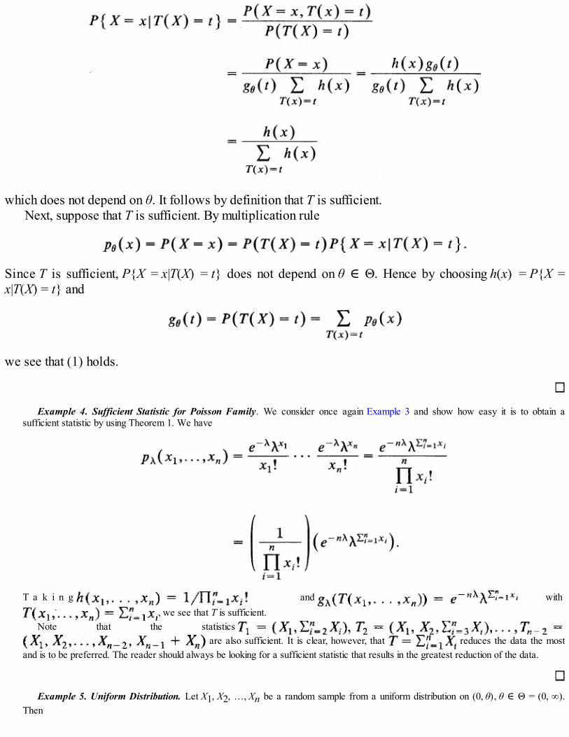
which does not depend on θ. It follows by definition that T is sufficient.Next, suppose that T is sufficient. By multiplication rule

Since T is sufficient, P{X = x|T(X) = t} does not depend on θ ∈ Θ. Hence by choosing h(x) = P{X =x|T(X) = t} and

we see that (1) holds.

Example 4. Sufficient Statistic for Poisson Family. We consider once again Example 3 and show how easy it is to obtain asufficient statistic by using Theorem 1. We have

T a k i n g and with , we see that T is sufficient.

Note that the statistics are also sufficient. It is clear, however, that reduces the data the most

and is to be preferred. The reader should always be looking for a sufficient statistic that results in the greatest reduction of the data.

Example 5. Uniform Distribution. Let X1, X2, …, Xn be a random sample from a uniform distribution on (0, θ), θ ∈ Θ = (0, ∞).Then

In cases such as this, where the domain of definition of fθ depends on θ, great care is needed. We use the following device to write fθ inone piece without the “if” part.

Let A be any set. Define the indicator function of A by

Indicator functions have simple properties, and the most useful property we need is the following:

We rewrite fθ(x1, …, xn) as follows

Now 0 < xi, < θ, i = 1, 2, …, n if and only if 0 < max(x1, …, xn) > θ. Hence

Choosing

and

we see that max(X1, …, Xn) is sufficient for θ.If, on the other hand, the common density of the Xi’s is

then

and

Since

it follows that

and choosing

and

we see that T is sufficient for θ. Here the vector (min Xi, max Xi) is jointly sufficient for the scalar parameter θ. We need to know bothmin Xi and max Xi. The knowledge of only one of the two is not sufficient.

Example 6. Sufficient Statistic for Normal Family. Let X1, X2, …, Xn be a random sample from a normal distribution with mean μ

and variance σ2. Suppose both μ and σ2 are unknown. Then and

we see that T is sufficient. If σ2 is not known, is not sufficient for μ. Similarly, if μ is not known, is not sufficient

for σ2. If σ2 is known, the same factorization shows that is sufficient for μ. If μ is known, we see easily from

that is sufficient for σ2. We emphasize that is computable from the observation (x1, …, xn)once μ is known.

It is possible to write in a more recognizable form. Knowledge of T is equivalent tothat of and . That is, if we know T we know and,

conversely, if we know we know T. It follows that is sufficient for (μ, σ2), which is reassuring.

Example 7*. Sufficient Statistic for a Nonparametric Family. Let be the class of all distribution functions on the real line thathave densities. Let X1, X2, …, Xn be a random sample from a distribution function F ∈ . Then the order statistic X(1) < X(2) < ⋯ <X(n) corresponding to the sample is sufficient for the family . A rigorous proof is beyond the scope of this text. Proceedingheuristically we note that each order statistic x(1) < x{2) < ⋯ < x(n) corresponds to n! n-tuples x1, x2, …, xn. That is, n! n-tuples x1, …,xn ∈ yield the same order statistic x(1) < x(2) < … < x(n). For example, the six triples (1.1, 1, 2.4), (11, 2.4, 1), (1, 11, 2.4), (1, 2.4,1.1), (2.4, 1, 1.1), (2.4, 11, 1) all yield the same order statistic 1 < 1.1 < 2.4. Since the observations are independent and identicallydistributed given (X(1), X(2), …, X(n)) = (X(1), X(2), …, X(n)), the conditional probability of observing any one of these n! n-tuples is 1/n!,which does not depend on the choice of F in .

We conclude this section with a few remarks. Suppose X1, X2, …, Xn is a random sample from somedistribution. Then any procedure that is based only on a part of the sample violates the criterion ofsufficiency and cannot be as good as the one based on the whole sample. Indeed, if the Xi’s are discrete,for example, then X1, X2, …, Xn – 1, say, is not sufficient. We have

which is not independent of the parameter.

Remark 1*. Since the object of looking for a sufficient statistic is to reduce the amount of data to becollected (without losing any information about the parameter that the sample contains) one should alwaysbe on the lookout for that sufficient statistic which results in the greatest reduction of data collection. Sucha statistic is called a minimal sufficient statistic. We will not give a formal definition of a minimalsufficient statistic here, but the following informal discussion will be helpful.

We recall that every random variable (and hence also every statistic) partitions the sample space. Let be the set of values of (X1, X2, …, Xn) and let T(X1, X2, …, Xn) be a statistic. Then T = T(X1, X2, …,

Xn) partitions into disjoint sets At = {(x1, x2, …, xn): T(x1, x2, …, xn) = t} where t a point in the rangeof T. Thus . A minimal sufficient statistic is one which induces on the coarsest partition inthe sense that if T1 is any other sufficient statistic then the partition sets induced by T1 are subsets of thoseinduced by T. For example, in Example 1 we saw that and are bothsufficient for p. However, T is preferable over T1 since it requires less data collection. For convenience,take n = 4. Then or 1, i = 1, 2, 3, 4} has 24 = 16 sample points.Partition sets induced by T are A = or 1 for each i}, t = 0, 1,…, 4. On the other hand, T1 induces a partition with sets

where Thus

and so on. It is now clear that {At} is coarser than {Bx1, t – x1} (see Figure 1).

If n(A) denotes the number of elements in set A. then clearly

Figure 1

whereas

and

Problems for Section 10.2

1. Use the definition of sufficiency to show that the statistic T = T(X1, X2, …, Xn) is sufficient for θ.

2. Let X1 and X2 be independent random variables, each having Poisson distribution with mean λ. Showthat X1 + 2X2 is not sufficient for λ.

3. Let X1 and X2 be independent random variables with P(X1 = 1) = p = 1 – P(X1 = 0), and P(X2 = 1) =5p = 1 – P(X2 = 0), 0 ≤ p ≤ 1/5. Is X1 + X2 sufficient for p? Is X1 + 3 X2 sufficient for p?

4. Let X1 and X2 be independent Bernoulli random variables with P(Xi = 1) = p = 1 – P(Xi = 0), 0 ≤ p <1. Show that X1 + X2 and X1 + 5X2 are both sufficient for p. Which of the two statistics is preferred??

5. Let X1, X2, …, Xn be a random sample of size n from a distribution with density fθ(x) given below.Find a sufficient statistic for θ by using factorization theorem.

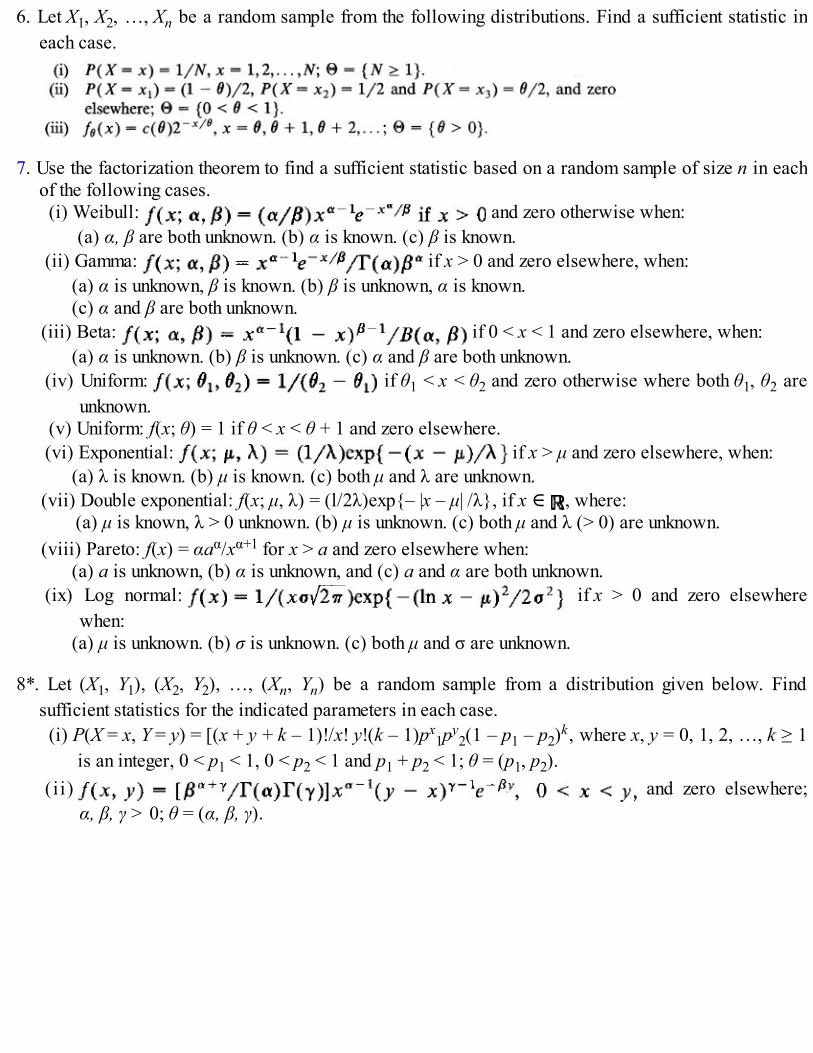
6. Let X1, X2, …, Xn be a random sample from the following distributions. Find a sufficient statistic ineach case.

7. Use the factorization theorem to find a sufficient statistic based on a random sample of size n in eachof the following cases.(i) Weibull: and zero otherwise when:

(a) α, β are both unknown. (b) α is known. (c) β is known.(ii) Gamma: if x > 0 and zero elsewhere, when:

(a) α is unknown, β is known. (b) β is unknown, α is known.(c) α and β are both unknown.

(iii) Beta: if 0 < x < 1 and zero elsewhere, when:(a) α is unknown. (b) β is unknown. (c) α and β are both unknown.

(iv) Uniform: if θ1 < x < θ2 and zero otherwise where both θ1, θ2 areunknown.

(v) Uniform: f(x; θ) = 1 if θ < x < θ + 1 and zero elsewhere.(vi) Exponential: if x > μ and zero elsewhere, when:

(a) λ is known. (b) μ is known. (c) both μ and λ are unknown.(vii) Double exponential: f(x; μ, λ) = (l/2λ)exp{– |x – μ| /λ}, if x ∈ , where:

(a) μ is known, λ > 0 unknown. (b) μ is unknown. (c) both μ and λ (> 0) are unknown.(viii) Pareto: f(x) = αaα/xα+1 for x > a and zero elsewhere when:

(a) a is unknown, (b) α is unknown, and (c) a and α are both unknown.(ix) Log normal: if x > 0 and zero elsewhere

when:(a) μ is unknown. (b) σ is unknown. (c) both μ and σ are unknown.

8*. Let (X1, Y1), (X2, Y2), …, (Xn, Yn) be a random sample from a distribution given below. Findsufficient statistics for the indicated parameters in each case.(i) P(X = x, Y = y) = [(x + y + k – 1)!/x! y!(k – 1)px

1py2(1 – p1 – p2)k, where x, y = 0, 1, 2, …, k ≥ 1

is an integer, 0 < p1 < 1, 0 < p2 < 1 and p1 + p2 < 1; θ = (p1, p2).(i i) and zero elsewhere;

α, β, γ > 0; θ = (α, β, γ).

(iii)

9. Let T(X1, …, Xn) be sufficient for θ where both T and θ are scalars. Let f be a one-to-one function on with inverse f–1.(i) Show that f(T) is sufficient for θ.(ii) Let d be a one-to-one function on . Show that T is sufficient for d(θ).

[Hint: Use factorization theorem. The results hold when either or both T and θ are vectors.]

10. Let T1 and T2 be two distinct sufficient statistics for θ. Show that T1 is a function of T2. Does it followthat every function of a sufficient statistic is itself sufficient?[Hint: Use factorization theorem. Is sufficient for μ, in sampling from a normal population?]

11. If T = ϕ(U) and T is sufficient for θ then so is U.

12. If T is sufficient for θ ∈ Θ, then it is also sufficient for θ ∈ ω ⊆ Θ.

[Hint: Use definition of sufficiency.]

10.3 UNBIASED ESTIMATION

Let X1, X2, …, Xn be a random sample from a distribution function Fθ, θ ∈ Θ ∈ . We recall (Section4.3) that an estimate T(X1, …, Xn) of θ is said to be unbiased for θ if |T| < ∞ and

We have subscripted by θ to indicate that the distribution function to be used in computation of theexpected value in (1) is Fθ. Thus, in the discrete case:

Then (1) is simply a property of the estimate that may be used to restrict our search to only those estimateswhich satisfy (1). An estimate T that does not satisfy (1) is called a biased estimate. We defined bias of Tby

For an unbiased estimate T, b(T, θ) = 0 for every θ ∈ Θ. Bias arises due to systematic error andmeasures, on the average, how far away and in what direction θT is from the parameter θ.

Example 1. Nonparametric Unbiased Estimates for Population Moments. Let X1, X2, …, Xn be a random sample from adistribution F ∈ which has finite k th moment . Nothing else is known or assumed about F. Thus = {F:

mk(F) finite}. Then the k th sample moment is unbiased for mk(F) since

by Theorem 5.3.1. In particular, is unbiased for μF, the population mean. Moreover, we have seen in Section 5.3 that S2 is unbiasedfor , the variance of F. See also Problem 5.4.4.

Frequently, however, there will be many unbiased estimates for a parameter. For example, if Xi, = μ= var(Xi) = σ2 (which is the case when Xi’s have a common Poisson distribution), then both and S2 areunbiased for μ as is also the estimate

since

Which of these should we choose? Moreover, the property of unbiasedness by itself is not enough. Wealso need to have a procedure to measure the precision of an estimate. An unbiased estimate with adistribution highly concentrated near θ should be preferable to the one with a distribution that is veryspread out. In Section 4.3 we said that the precision of any estimate T (biased or unbiased) for θ ismeasured by its mean square error (MSE) defined by

We recall that

In particular, if b(T, θ) = 0, then T is unbiased for θ and MSEθ(T) = varθ(T). Recall also that an estimateT1 for θ is preferable to an estimate T2 (for θ) if

with strict inequality holding for at least one θ in Θ. For unbiased estimates T1 and T2, (5) reduces to

with strict inequality for at least one θ in Θ. If there exists an unbiased estimate for θ which has thesmallest variance amongst all unbiased estimates it is called a uniformly minimum variance unbiasedestimate (UMVUE) for θ. Thus T is UMVUE of θ if

and

How does sufficiency fit in here? Intuitively, if there are two unbiased estimates for θ the one basedon a sufficient statistic should be preferable to the one that is not based on a sufficient statistic. It wouldappear therefore that we need only concentrate on estimates based on sufficient statistics. If so, does itmean that an estimate based on a sufficient statistic necessarily has a smaller variance than an estimatethat is not based on a sufficient statistic? The answer is yes, but let us first consider some examples.

Example 2. Estimating Variance of a Normal Distribution. Let X1, X2, …, Xn be a random sample from a normal distribution with

unknown mean μ and unknown variance σ2. Suppose we wish to estimate σ2. We know that S2 is always unbiased for σ2. Suppose,however, that biasedness of an estimate for σ2 is not a drawback. Rather, we prefer an estimate that has a smaller MSE. Consider allestimates of the form Tc = cS2 where c > 0 is a constant to be determined. We will find one estimate having the least MSE in the class

{Tc: c σ 0}. Since (n – 1)S2/σ has a chi-square distribution with (n – 1) d.f. (Theorem 8.7.1), we note that

so that

Now

and from (4)

Let

Then m(c) is minimized for c = c0 given by

provided that . We have

which yields c0 = (n – 1)/(n + 1). Moreover,

It follows that

has the smallest MSE in the class of all estimates {cS2 : c < 0}. We note that

so that Tc0 is negatively biased for σ2 (tends to underestimate σ2). Moreover, Tc0

is based on the sufficient statistic for σ2

(when μ is unknown).

Example 3. Estimating p2 for Bernoulli Distribution. Let X1, X2, …, Xn be a sample from a Bernoulli distribution with parameter

p, 0 ≤ p ≤ 1. First suppose that n = 1. Can we estimate p2 unbiasedly based on one observation? The answer is no. To see this, let T(X)be an estimate of p2. If T is unbiased, then

Since (8) is true for all p, the coefficient of various powers of p on both sides of (8) must be the same. This being impossible, no such Texists.

Suppose now that n < 1. Can we estimate p2 unbiasedly and if so how? We note that is sufficient for p and hasa binomial distribution with

Since (T/n) = p, T/n is unbiased for p and since p2 = p.p, (T/n)2 appears to be a candidate. But (T/n)2 cannot be unbiased for p2. Thisis typical of unbiased estimates. If T is unbiased for θ, f(T) is not in general unbiased for f(θ) (except when f is a linear function of θ).Integrals and sums simply do not behave that nicely. In our example?

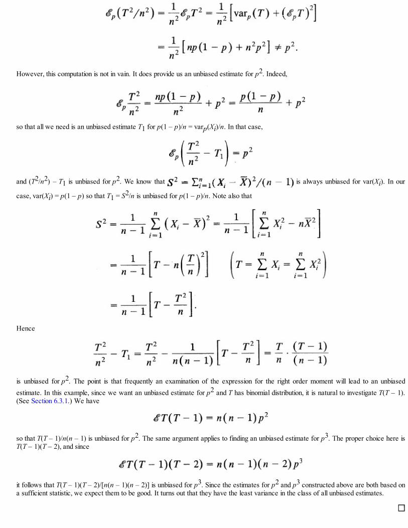
However, this computation is not in vain. It does provide us an unbiased estimate for p2. Indeed,

so that all we need is an unbiased estimate T1 for p(1 – p)/n = varp(Xi)/n. In that case,

and (T2/n2) – T1 is unbiased for p2. We know that is always unbiased for var(Xi). In our

case, var(Xi) = p(1 – p) so that T1 = S2/n is unbiased for p(1 – p)/n. Note also that

Hence

is unbiased for p2. The point is that frequently an examination of the expression for the right order moment will lead to an unbiasedestimate. In this example, since we want an unbiased estimate for p2 and T has binomial distribution, it is natural to investigate T(T – 1).(See Section 6.3.1.) We have

so that T(T – 1)/n(n – 1) is unbiased for p2. The same argument applies to finding an unbiased estimate for p3. The proper choice here isT(T – 1)(T – 2), and since

it follows that T(T – 1)(T – 2)/[n(n – 1)(n – 2)] is unbiased for p3. Since the estimates for p2 and p3 constructed above are both based ona sufficient statistic, we expect them to be good. It turns out that they have the least variance in the class of all unbiased estimates.

Example 4. Taxi Problem Revisited . Let X1, X2, …, Xn be a random sample from the uniform distribution on {1, 2, …, N}. InSection 6.2 we considered several estimates of N (Example 6.2.1, Problem 6.2.7). Here the parameter is N and takes values in Θ = {allintegers ≥ 2}. We note that

so that is unbiased for N. We showed in Example 6.2.1 that 2 = (n + 1)Mn/n is nearly unbiased for N but is notunbiased. In Problem 6.2.7 we showed that 3 = Mn + Nn – 1 is unbiased for N. [Here Mn = max(X1, …, Xn) and Nn = min(X1, …,Xn).] We note that Mn is sufficient for N so that 2 should be preferable over 1. Is MSE( 2) < MSE( 1)? We note that

and it is possible to show by approximating the sums by integrals (as was done in Example 6.2.1) that

We have

What about 3? Computation of MSE (or variance) of 3 is messy. So we argue as follows. The estimate 3 is not based on the“best” sufficient statistic Mn. Hence we should not expect it to perform better than 2. Since Mn is sufficient for N, an unbiasedestimate based on Mn should perform well in terms of its variance. It turns out that the estimate

based on Mn is unbiased for N and has the least variance among all unbiased estimates for N. We will not prove this assertion.

Unbiasedness and Sufficiency

Let T1(X1, …, Xn) and T2(X1, …, Xn) be two unbiased estimates for a parameter θ. Let T(X1, …, Xn) besufficient for θ. Suppose T1 = f(T) for some function f. If sufficiency of T for θ is to have any meaning, weshould expect T1 to perform better than T2 in the sense that var(T1) ≤ var(T2). Otherwise there would beno reason to study sufficiency. More generally, given an unbiased estimate h for θ, is it possible toimprove upon h by using a sufficient statistic for θ? The answer is yes. Suppose T is sufficient for θ. Thenthe conditional distribution of (X1, …, Xn) given T does not depend on θ. Consider θ{h(X1, …, Xn)|T(X1,…, Xn)}. Since the expected value is computed with respect to the conditional distribution of (X1, …, Xn)given T it also does not depend on θ. Hence

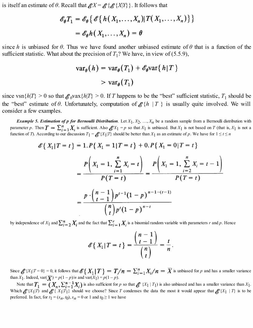
is itself an estimate of θ. Recall that X = { {X|Y}}. It follows that

since h is unbiased for θ. Thus we have found another unbiased estimate of θ that is a function of thesufficient statistic. What about the precision of T1? We have, in view of (5.5.9),

since vsn{h|T} > 0 so that θvax{h|T} > 0. If T happens to be the “best” sufficient statistic, T1 should bethe “best” estimate of θ. Unfortunately, computation of {h | T } is usually quite involved. We willconsider a few examples.

Example 5. Estimation of p for Bernoulli Distribution. Let X1, X2, …, Xn be a random sample from a Bernoulli distribution withparameter p. Then is sufficient. Also X1 = p so that X1 is unbiased. But X1 is not based on T (that is, X1 is not afunction of T). According to our discussion T1 = {X1|T} should be better than X1 as an estimate of p. We have for 1 ≤ t ≤ n

by independence of X1 and and the fact that is a binomial random variable with parameters r and p. Hence

Since {X1|T = 0} = 0, it follows that is unbiased for p and has a smaller variancethan X1. Indeed, var( ) = p(1 – p)/n and var(X1) = p(1 – p).

Note that is also sufficient for p so that {X1 | T1) is also unbiased and has a smaller variance than X1.Which {X1|T) and { X1|T1} should we choose? Since T condenses the data the most it would appear that {X1 | T} is to bepreferred. In fact, for t1 = (xn, t0), xn = 0 or 1 and t0 ≥ 1 we have

by independence. It follows that is also unbiased for p and has smaller variance than X1. Since

we see that is to be preferred. Thus, even though every sufficient statistic will yield a better estimate for p than X1, the estimate basedon a sufficient statistic that reduces the data the most (minimal sufficient statistic) is the one to look for. This result is true in general but itis beyond our scope to prove it.

Example 6. Estimation of Exponential Mean. Let X1, X2, …, Xn be a random sample from an exponential density function withmean θ. Then is sufficient for θ. To estimate θ, therefore, all we need to do is find an unbiased estimate based on .This is given by . In fact, is the best unbiased estimate of θ, but we cannot prove it here. This is related to the fact that isthe “best” sufficient statistic.

To estimate θ2, for example, we note that var(X) = θ2 so that S2, the sample variance, is an unbiased estimate for θ2. But S2 is notbased on (or ) so that it should perform worse than an unbiased estimate based on . Is there such an estimate?It is natural to compute . We have

It follows that is unbiased for θ, which is a function of the sufficient statistic . It turns out to be the unbiased

estimate for θ2 with the least variance.

The procedure for finding unbiased estimates with smaller variance can now be summarized:

(i) Find, if possible, a sufficient statistic that reduces the data the most.(ii) Find a function of this sufficient statistic that is unbiased by trial and error.(iii) If your sufficient statistic is the best possible (minimal), then your unbiased estimate will have the

least variance. If not, the unbiased estimate you construct will not be the best possible but you havethe assurance that it is based on a sufficient statistic.

Example 7. Estimation of Mean and Variance of a Nonparameteric Family . In Example 1 we considered the unbiasedestimation of μ and σ2 without any restrictions on F. Let be the family of all distribution functions on the real line which have densitiesand finite mean and finite variance. In Example 10.2.7 we argued that the ordered statistic X(1) < X(2) < ⋯ < X(n) based on a random

sample from F ∈ is sufficient. In Example 1 of this section we saw that and so that and S2 are

unbiased estimates of μ and σ2. Since

and

are both functions of the sufficient statistic (X(1), …, X(n)) we should be confident that these are good estimates of μ and σ2 respectively,certainly better than unbiased estimates not based on (X(1), …, X(n)) since it is the best sufficient statistic.

Example 8. Empirical Distribution Function. Let X1, X2, …, Xn be a random sample from a continuous population distributionfunction F ∈ with density f. Then the order statistic X(1) < X(2) < X(n) is sufficient (Example 10.2.7). We show that the empiricaldistribution function defined by

is a function of the order statistic and is unbiased for F. Indeed, we can rewrite

where ε(x) = 1 if x > 0 and zero otherwise. Moreover,

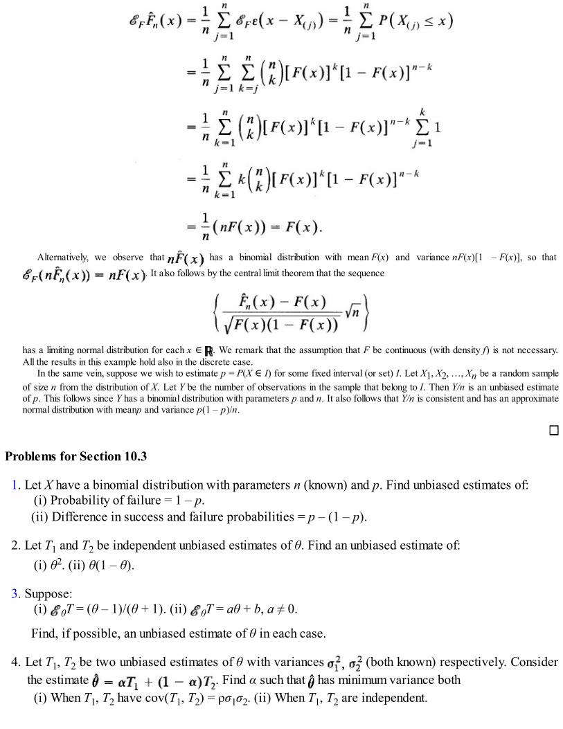
Alternatively, we observe that has a binomial distribution with mean F(x) and variance nF(x)[1 – F(x)], so that . It also follows by the central limit theorem that the sequence

has a limiting normal distribution for each x ∈ . We remark that the assumption that F be continuous (with density f) is not necessary.All the results in this example hold also in the discrete case.

In the same vein, suppose we wish to estimate p = P(X ∈ I) for some fixed interval (or set) I. Let X1, X2, …, Xn be a random sampleof size n from the distribution of X. Let Y be the number of observations in the sample that belong to I. Then Y/n is an unbiased estimateof p. This follows since Y has a binomial distribution with parameters p and n. It also follows that Y/n is consistent and has an approximatenormal distribution with meanp and variance p(1 – p)/n.

Problems for Section 10.3

1. Let X have a binomial distribution with parameters n (known) and p. Find unbiased estimates of:(i) Probability of failure = 1 – p.(ii) Difference in success and failure probabilities = p – (1 – p).

2. Let T1 and T2 be independent unbiased estimates of θ. Find an unbiased estimate of:(i) θ2. (ii) θ(1 – θ).

3. Suppose:(i) θT = (θ – 1)/(θ + 1). (ii) θT = aθ + b, a ≠ 0.

Find, if possible, an unbiased estimate of θ in each case.

4. Let T1, T2 be two unbiased estimates of θ with variances (both known) respectively. Considerthe estimate . Find α such that has minimum variance both

(i) When T1, T2 have cov(T1, T2) = ρσ1σ2. (ii) When T1, T2 are independent.

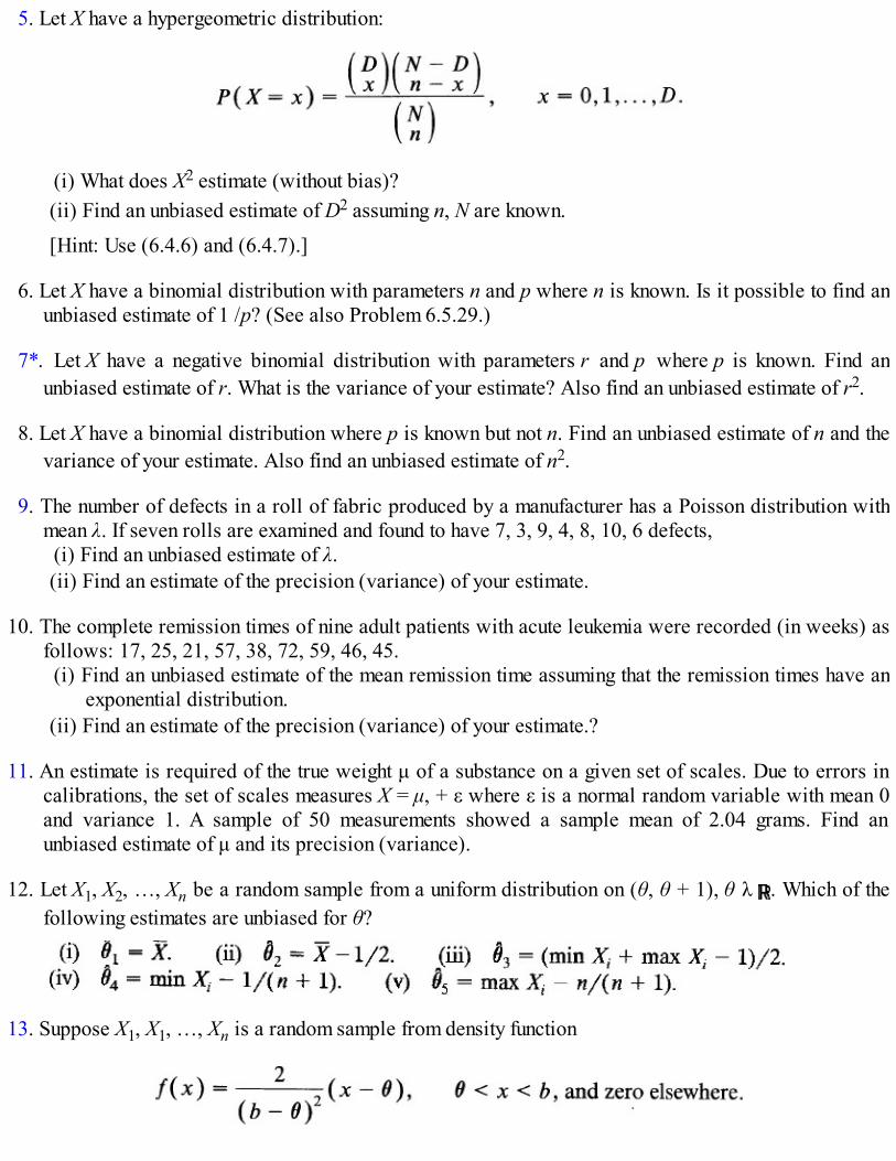
5. Let X have a hypergeometric distribution:

(i) What does X2 estimate (without bias)?(ii) Find an unbiased estimate of D2 assuming n, N are known.

[Hint: Use (6.4.6) and (6.4.7).]

6. Let X have a binomial distribution with parameters n and p where n is known. Is it possible to find anunbiased estimate of 1 /p? (See also Problem 6.5.29.)

7*. Let X have a negative binomial distribution with parameters r and p where p is known. Find anunbiased estimate of r. What is the variance of your estimate? Also find an unbiased estimate of r2.

8. Let X have a binomial distribution where p is known but not n. Find an unbiased estimate of n and thevariance of your estimate. Also find an unbiased estimate of n2.

9. The number of defects in a roll of fabric produced by a manufacturer has a Poisson distribution withmean λ. If seven rolls are examined and found to have 7, 3, 9, 4, 8, 10, 6 defects,

(i) Find an unbiased estimate of λ.(ii) Find an estimate of the precision (variance) of your estimate.

10. The complete remission times of nine adult patients with acute leukemia were recorded (in weeks) asfollows: 17, 25, 21, 57, 38, 72, 59, 46, 45.

(i) Find an unbiased estimate of the mean remission time assuming that the remission times have anexponential distribution.

(ii) Find an estimate of the precision (variance) of your estimate.?

11. An estimate is required of the true weight μ of a substance on a given set of scales. Due to errors incalibrations, the set of scales measures X = μ, + ε where ε is a normal random variable with mean 0and variance 1. A sample of 50 measurements showed a sample mean of 2.04 grams. Find anunbiased estimate of μ and its precision (variance).

12. Let X1, X2, …, Xn be a random sample from a uniform distribution on (θ, θ + 1), θ λ . Which of thefollowing estimates are unbiased for θ?

13. Suppose X1, X1, …, Xn is a random sample from density function

Find an unbiased estimate of θ when b is known. [Hint: Find X.]

14. Let X1, X2, …, Xn be n independent and identically distributed random variables with commonuniform distribution on [0, θ]. Find an unbiased estimate of θα based on the sufficient statistics X(n) =max(X1, …, Xn). (Here α is known.) [Hint: What is ]

15. Let X1, …, Xn be a random sample from density function f(x) = 2(θ … x)/θ2, 0 ≤ x ≤ θ, and zeroelsewhere. Find an unbiased estimate of θ.

16. Suppose X has a Bernoulli distribution with parameter θ2. That is,

Show that there exists no unbiased estimate of θ.

17. Let X have a Poisson distribution with mean λ. Let θ = 1/λ. Show that there does not exist an unbiasedestimate of θ.

18. Let X1, X1, …,Xn be a random sample from a Bernoulli distribution with parameter p. Let 0 < r < n bean integer. Find unbiased estimates of:

(i) d(p) = pr. (ii) d(p) = pr + (1 – p)n – r.

19. Let X1, X2, …, Xn be a random sample from a normal distribution with unknown mean μ and unknownvariance σ2. Find an unbiased estimate of ζp the quantile of order p where

based on the sufficient statistic .

[Hint: Standardize and find the relation between μ, σ and ζp. Use (8.7.2).]

20. An example where an unbiased estimate may not be desirable (see Example 8.5.2): Let X1, X2, …, Xnbe the survival times (in months) of n patients with advanced lung cancer. Suppose Xi’s areindependent, having a common exponential distribution with mean λ < 0. The object of the study is toestimate λ and an unbiased estimate is desired. Show that

are both unbiased estimates of λ.If smaller variance is the criterion used, which of the two would you choose?In particular, consider the sample survival times (in months) 4, 77, 55, 4, 14, 23, 110, 10, 9, 62,

and compare the two estimates and their precisions.

21. Let X1, X2, …, Xn be independent and identically distributed random variables with common Poissondistribution with mean λ. Find an unbiased estimate for d(λ) where:

(i) d(λ) = λ2. (ii) d(λ) = λ3. (iii) d(λ) = λk, k ≥ 1 integral, k ≤ n.

[Hint: Consider product moments. See also Problem 10.8.9.]

22. Let X1, X2, …, Xn be independent Bernoulli random variables with common parameter p. Find anunbiased estimate of pk (k ≥ 1 integral k < n) based on a sufficient statistic. [Hint: Consider productmoments. Follow Example 5.]

23*. The number of accidents X per year in a plant may be modeled as a Poisson random variable withmean λ. Assume that the accidents in successive years are independent random variables and supposeyou have n observations. How will you find a good unbiased estimate for the probability e–λ that inany given year the plant has no accidents? [Hint: Define Yi = 1 if Xi = 0 and Yi = 0 otherwise. Then Yiis unbiased. Find {Yi|T} where T is a sufficient statistic.]

24*. In Problem 23, suppose we wish to estimate λ.(i) Show that and S2 are both unbiased for λ.(ii) Note that is sufficient for λ. Which of the two unbiased estimates would you choose if your

estimate is to have smaller variance? (Do not compute variance of S2.)(iii) Show that and hence conclude that var( ) ≤ var(S2). [Hint:

. The conditionaldistribution of Xi given is binomial, with parameters t and 1/n (Problem 8.8.17).]

25*. Let X1, X2, …, Xn be a random sample from a normal distribution with mean θ and variance θ. Thennecessarily θ > 0 and both and S2 are unbiased for θ.

(i) Which of the two estimates is preferable?(ii) Is either or S2 a function of the “best” sufficient statistic?

26. Let X1, X2, …, Xn be a random sample from a population distribution with mean μ and variance σ2.Let .

(i) Show that Sn is an unbiased estimate of μ if .(ii) Consider the class of all unbiased estimates of μ of the form Sn where a1, …, an ∈ are such

that . Show that the estimate with the least variance in this class is given by ai =1/n, i = 1, …, n. [Hint: Note that implies that

.]

10.4 THE SUBSTITUTION PRINCIPLE (THE METHOD OF MOMENTS)

One of the simplest and oldest methods of estimation is the substitution principle: Let d(θ), θ ∈ Θ be aparametric function to be estimated on the basis of a random sample X1, X2, …, Xn from a populationdistribution function F. Suppose d can be written as d(θ) = h(F) for some function h. Then the substitutionprinciple estimate of d(θ) is h( ) where is the empirical distribution function defined by

(See Section 4.5.) This method leads to estimates that are quickly and easily computed. Often estimateshave to be computed by some numerical approximation procedure. In that case this method provides a

preliminary estimate.

Example 1. Estimating the Average Number of Blood-Spotted Eggs in a Flock of Chickens . The following problem hasattracted wide attention in the literature. A poultry scientist wishes to estimate the frequency of occurrence of blood-spotted eggs for aflock by observing a small number of eggs laid early in the life of each hen.

Let p be the probability that a given chicken will lay a blood-spotted egg and let m be the number of eggs laid. The number of blood-spotted eggs X is assumed to have a binomial distribution with parameters m and p. The probability p, however, varies from chicken tochicken and can be thought of as having a continuous distribution on (0, 1). This probability distribution is not observable. We assume thatthe distribution function of p is F (with density function f) and that the values of p for each bird in the flock are independently assignedaccording to the distribution F (although these values are not observed). Thus the conditional distribution of X is binomial and theunconditional distribution is given by

The problem is to estimate

the average probability of laying a blood-spotted egg for the flock.Let us digress a little to consider the problem of estimating the /cth moment of a distribution function X. The substitution

principle says that is an estimate of . Since assigns probability 1/n to each of X1, X2, …, Xn

is the k th sample moment. Thus a moment of any order is estimated by the sample moment of the same order. Hence the name methodof moments.

Returning to the problem at hand, we note that

so that

By the substitution principal, therefore, we estimate μF by where

where X1, X2, …, Xn is a random sample on X. We note that

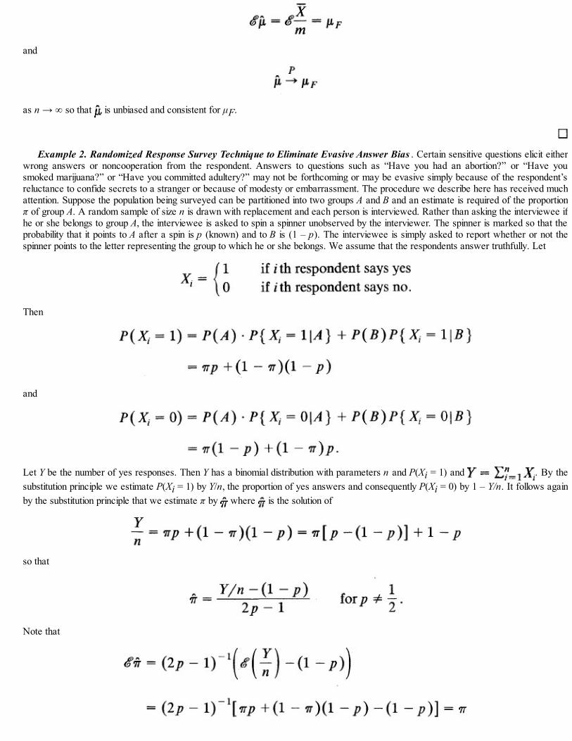
and

as n → ∞ so that is unbiased and consistent for μF.

Example 2. Randomized Response Survey Technique to Eliminate Evasive Answer Bias . Certain sensitive questions elicit eitherwrong answers or noncooperation from the respondent. Answers to questions such as “Have you had an abortion?” or “Have yousmoked marijuana?” or “Have you committed adultery?” may not be forthcoming or may be evasive simply because of the respondent’sreluctance to confide secrets to a stranger or because of modesty or embarrassment. The procedure we describe here has received muchattention. Suppose the population being surveyed can be partitioned into two groups A and B and an estimate is required of the proportionπ of group A. A random sample of size n is drawn with replacement and each person is interviewed. Rather than asking the interviewee ifhe or she belongs to group A, the interviewee is asked to spin a spinner unobserved by the interviewer. The spinner is marked so that theprobability that it points to A after a spin is p (known) and to B is (1 – p). The interviewee is simply asked to report whether or not thespinner points to the letter representing the group to which he or she belongs. We assume that the respondents answer truthfully. Let

Then

and

Let Y be the number of yes responses. Then Y has a binomial distribution with parameters n and P(Xi = 1) and . By thesubstitution principle we estimate P(Xi = 1) by Y/n, the proportion of yes answers and consequently P(Xi = 0) by 1 – Y/n. It follows againby the substitution principle that we estimate π by where is the solution of

so that

Note that

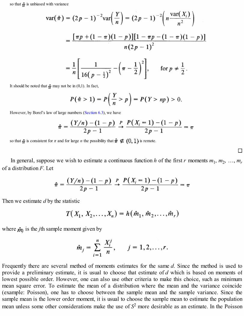
so that is unbiased with variance

It should be noted that may not be in (0,1). In fact,

However, by Borel’s law of large numbers (Section 6.3), we have

so that is consistent for π and for large n the possibility that is remote.

In general, suppose we wish to estimate a continuous function h of the first r moments m1, m2, …, mrof a distribution F. Let

Then we estimate d by the statistic

where j is the jth sample moment given by

Frequently there are several method of moments estimates for the same d. Since the method is used toprovide a preliminary estimate, it is usual to choose that estimate of d which is based on moments oflowest possible order. However, one can also use other criteria to make this choice, such as minimummean square error. To estimate the mean of a distribution where the mean and the variance coincide(example: Poisson), one has to choose between the sample mean and the sample variance. Since thesample mean is the lower order moment, it is usual to choose the sample mean to estimate the populationmean unless some other considerations make the use of S2 more desirable as an estimate. In the Poisson

case, it can be shown that var( ) ≤ var(S2) so that would be the choice to estimate Xi if smallervariance was desired.

The method of moments estimates are consistent under mild conditions and have an asymptotic normaldistribution.

Example 3. Estimating the Number of Taxis in a Town . In Example 6.2.1 we considered several estimates of N in sampling fromthe probability function

To find the substitution principle estimate of N we note that

so that N = 2 X – 1. By the substitution principle we estimate N by

where is the sample mean of a sample of size n. We note that Ñ is unbiased and consistent and by the central limit theorem

for all x ∈ (– ∞, ∞). Here σN = {(N2 – 1)/12}1/2 (Problem 6.2.1).We note that Ñ is not based on the sufficient statistic max(X1, …, Xn). In this case we said in Example 10.3.4 that the best unbiased

estimate of is a function of Mn = max(X1, …, Xn) and is given by

We note that the method of moments estimate of

given by

is a nonparametric estimate since it does not depend on the form of F. Similarly, if an estimate of amedian of X is desired, it is the sample median. Indeed, by definition median of X is a number m such that

so that by substitution principle the estimate of m satisfies

Hence it is the sample median, given by

Problems for Section 10.4

1. Let X1, X2, …, Xn be a sample from a Bernoulli population with parameter p.(i) Show that is a method of moments estimator of p.(ii) Find a method of moments estimate of var(X1) = p(1 – p) based only on .(iii) Find a method of moments estimate of var(X1) = p(1 – p) based on the second sample moment.(iv) Show that the estimates in (ii) and (iii) are identical. [Hint: P(Xi = 1) = p, P(Xi = 0) = 1 – p so

.]

2. In a clinical trial n patients with advanced cancer of the prostate survived times t1, t2, …, tn (months).Suppose that the survival distribution is exponential with? mean λ:

(i) Find two different method of moments estimates of λ.(ii) Find a method of moment estimate of the survival function

(iii) If n = 8 and the survival times were recorded (in months) as 9, 15, 8, 25, 6, 17, 23, 5 find theseestimates. In part (ii) take t = 20.

3. A certain blood disease occurs in a proportion p of white females. A random sample of n femaleswas selected and it was found that X females in the sample have the blood disease. Unfortunately, theresearcher lost track of the total number n of females surveyed. Find the method of moments estimateof n if p is known.

4. How will you estimate the proportions of freshmen, sophomores, juniors, and seniors at a large stateuniversity based on a sample of size n?

5. Heritable characteristics depend on genes, which are passed on from parents to offsprings. Genesappear in pairs, and in the simplest case each gene of a particular pair can assume one of two formscalled alleles, A and a. Therefore, there are three possible genotypes: AA, Aa, and aa. (Biologically,there is no difference between aA and Aa.) According to the Hardy–Weinberg stability principle thegenotype probabilities stabilize after one generation in a population with random mating (seeProblems 6.7.15 and 6.7.16). We are therefore led to assume that after one generation there are threetypes of individuals with proportions

Let Xi be the number of individuals of type i in a sample of n individuals. How will you estimate pby method of moments?

6. The diameters of a large shipment of ball bearings have a normal distribution with mean μ andvariance σ2. A sample of size n is taken. Find estimates for μ, σ2, and σ.

7*. The lead time for orders of diodes from a certain manufacturer has a gamma distribution with mean μand standard deviation σ. Estimate the parameters of the gamma distribution based on a sample ofsize n.

8*. The proportion of defective tires manufactured by a certain company has a beta distribution withparameters α and β. Estimate α and β based on a sample of n proportions.

9*. Let X1, X2, …, Xn be a sample from a negative binomial distribution with parameters p and r, 0 < p <1, and r ≥ 1 integral. Find estimates of r and p.

10. Let ζp be the pth percentile of a distribution function F so that ζp is a value satisfying

Find an estimate of ζp based on a sample of size n. Find also an estimate of the survival function S(t)= 1 – F(t).

11*. The lifetime of a mechanical part is a random variable with density function

Find an estimate of α and of the survival function S(t).

12. In Example 1 we considered defined by

as an estimate of in sampling from

Show that

and that is asymptotically normal with mean μF and variance vai(X1)/m2n for large n.

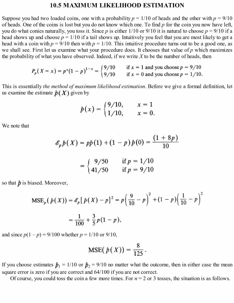
10.5 MAXIMUM LIKELIHOOD ESTIMATION

Suppose you had two loaded coins, one with a probability p = 1/10 of heads and the other with p = 9/10of heads. One of the coins is lost but you do not know which one. To find p for the coin you now have left,you do what conies naturally, you toss it. Since p is either 1/10 or 9/10 it is natural to choose p = 9/10 if ahead shows up and choose p = 1/10 if a tail shows up. Intuitively you feel that you are most likely to get ahead with a coin with p = 9/10 then with p = 1/10. This intuitive procedure turns out to be a good one, aswe shall see. First let us examine what your procedure does. It chooses that value of p which maximizesthe probability of what you have observed. Indeed, if we write X to be the number of heads, then

This is essentially the method of maximum likelihood estimation. Before we give a formal definition, letus examine the estimate given by

We note that

so that is biased. Moreover,

and since p(1 – p) = 9/100 whether p = 1/10 or 9/10,

If you choose estimates 1 = 1/10 or 2 = 9/10 no matter what the outcome, then in either case the meansquare error is zero if you are correct and 64/100 if you are not correct.

Of course, you could toss the coin a few more times. For n = 2 or 3 tosses, the situation is as follows.

In the case when n = 2 we have no difficulty in concluding that p = 1/10 if x = 0 and p = 9/10 if x = 2.But when x = 1, we cannot make a choice. The reason is that 1/10 = 1 – 9/10 so that if the coin is tossedan even number of times, the probability of n/2 successes and n/2 failures with both coins is the same,namely

In the case when n = 3, we see that our choice of p that maximizes the probability of observing x isgiven by

You can now see that the procedure we have used is the following: Given that the outcome is x,estimate p by a value ∈ Θ, which maximizes Pp(X = x).

This is all very well when X is the discrete type but what happens when X has a continuousdistribution? In that case, for any outcome x

We can argue as follows. If X = x is observed, the probability that the outcome x falls in an interval of(small) length dx around x is given by

where fθ is the density function of X. The above procedure can now be applied as follows: Estimate θ bythat value in Θ which maximizes fθ(x) so that the probability of the outcome falling in a smallneighborhood of x is maximum.

To formalize this idea, let (X1, X2, … Xn) be a random vector with joint density or probabilityfunction fθ(x1, …, xn) where θ ∈ Θ is the unknown parameter. Here θ may be a scalar or a vector.

DEFINITION 1. The likelihood function of the observation (x1, x2, … xn) is a function of θ defined onΘ by

In the discrete case L(θ; x1, …, xn) is just the probability of observing X1 = x1, …, Xn = xn. In thecontinuous case, however, we need a constant multiple of fθ(x1, …, xn) to represent the volume of a smallneighborhood of the observation (x1, …, xn) to give the same interpretation to the likelihood function.That is, technically

for some arbitrary constant c > 0. But we will take c = 1 as above.In the special case (of most interest) when X1, X2, …, Xn is a random sample?

Maximum Likelihood Principle

Choose as an estimate of θ a value that maximizes the likelihood function, that is, a satisfying

If such a exists, it is known as a maximum likelihood estimate of θ. In many practical problems,maximum likelihood estimates are unique although this is not true in general. Sometimes an observedvalue of (x1, …, xn) will produce a value of that is not in Θ. In that case we say that a maximumlikelihood estimate does not exist.

Since logarithm is a monotone function we note that

In the case of random sampling when L is of the form (1) it is convenient to work with the log likelihoodfunction. Often the likelihood function is differentiable in Θ. In that case we solve the likelihoodequation(s)

to find , but then we need to check if is indeed a maximum. (Check to see if )

Example 1. Maximum Likelihood Estimate of Poisson Mean–Wrong Telephone Connections . The number of connections to awrong number at a telephone exchange is frequently modeled by a Poisson distribution. Let x1, x2, …, xn be the observed number ofwrong connections on n different days. If we assume that the mean number of wrong connections is the same, namely λ, on each day andthat the events are independent, then

so that

It follows that

and

Hence

gives the maximum likelihood estimate as

provided that since . This problem is sometimes avoided by taking the parameter set to be theclosure of Θ.

We note that is unbiased and is a sufficient statistic for λ. Moreover is consistent for λ.In particular, if we observe 6, 5, 11, 2, 9, 7, 7, 6, 10 wrong connections on nine randomly chosen days at this exchange, then

. It means that the likelihood function, given this set of observations, namely

has a larger value for λ = = 7 than for any other λ ∈ Θ = (0, ∞). Moreover, no matter what the sample (of size 9), as long as = 7,the likelihood function is maximized at λ = 7.

Example 2. Estimating θ for Uniform Distribution. Suppose a bus arrives at a bus stop between time 0 and time θ (inclusive) andthat the probability of arrival in any subinterval of time is proportional to the length of the subinterval. Then the time X that a person whoarrives at time 0 has to wait for the bus has a uniform distribution on [0, θ]. In order to estimate θ suppose we take n independentobservations on X, say x1, x2,…,xn. What is the maximum likelihood estimate of θ? The likelihood function is given by

Here the domain of definition depends on θ so that 1/θn is not the joint density. If we were to differentiate In L(θ) blindly, we end up with

which gives = ∞, the minimum of L(θ). The likelihood function is in fact

where IA is the indicator function of set A. If we plot the likelihood function we get Figure 1. The maximum is at θ = max(x1,…,xn) andthe maximum likelihood estimate for θ is given by

The result is obtained if we observe that L(θ) is a strictly decreasing function of θ so that the maximum is achieved at the smallest possiblevalue of θ, namely, max(x1,…,xn).

We note that is consistent for θ but not unbiased (Example 8.5.4). Again is a sufficient statistic (in fact the best) for θ.

Example 3. Restricted Bernoulli Parameter. Suppose we take one observation from a Bernoulli distribution where we know that p∈ [1/3, 2/3]. Then the likelihood function is given by

A plot of L(p; x) is given in Figure 2. It is clear that the maximum of L(p; x) is achieved at p = 1/3 when x = 0 and at p = 2/3 when x = 1.It follows that the maximum likelihood estimate is given by

Figure 1

Figure 2

We can rewrite

and note that

so that is biased. Moreover,

Consider now the trivial estimate 1 = 1/2, which ignores the observation. The MSE of l is given by

for p ∈ [1/3, 2/3] and the maximum likelihood estimate is worse than the trivial estimate .

Example 4. Estimating Mean and Variance of a Normal Distribution . Let X1, X2,…,Xn be a random sample from a normal

distribution with mean θ and variance σ2. We first suppose that both θ and σ2 are unknown so that λ = (θ, σ2) ∈ {(θ, σ2): θ ∈ , σ2 > 0}.The likelihood function is given by

so that

Differentiating with respect to θ and σ2 we get

and

Solving ∂ In L/∂θ = 0 and ∂ In L/∂σ2 = 0 simultaneously gives maximum likelihood estimates

We leave the reader to show that do indeed give maxima for L(λ). We note that although is unbiased for is biasedsince

Moreover, both and are consistent estimates for θ and σ2 respectively, and is sufficient for (θ, σ2).If θ, is unknown and σ is known, the same argument leads to as the maximum likelihood estimate. If σ is unknown and θ is

known, the maximum likelihood estimate for σ2 is given by

We have thus far seen that a maximum likelihood estimate may not in general be unique, may not beunbiased, and appears to be consistent and a function of a sufficient statistic. Let us consider the last twoproperties and also the invariance property of maximum likelihood estimates.

Under some reasonable conditions it can be shown that the method of maximum likelihood estimationleads to a consistent estimate which has an asymptotic normal distribution. A proof of this property isbeyond our scope. However, this large sample property of maximum likelihood estimates is frequentlyvery useful.

PROPOSITION 1. (SUFFICIENCY AND MAXIMUM LIKELIHOOD ESTIMATES). Suppose X1,X2,…, Xn is a random sample from a discrete or a continuous type distribution. Let T(X1,…, Xn) be asufficient statistic for the parameter θ ∈ Θ. If there exists a unique maximum likelihood estimate of

θ, then is a (nonconstant) function of T. If a maximum likelihood estimate of θ exists but is notunique, then one can find a maximum likelihood estimate that is a function of T.

Proof. By factorization theorem,

for all x1,…, xn, θ, and some h and gθ. If a unique exists that maximizes L(θ), it also maximizes gθ(T(x1,…, xn)) and hence is a function of T. If a maximum likelihood estimate of θ exists but is not unique, wechoose a particular maximum likelihood estimate which is a function of T from the set of all maximumlikelihood estimates.

Example 5. Uniform Distribution on [Θ – 1, θ + 1]. Let X1, X1,…, Xn be a random sample from the uniform distribution on [θ – 1,θ + 1]. Then the likelihood function is given by

We note that T(X1,…, Xn) = (min Xi, max Xi) is jointly sufficient for θ. Now any θ satisfying

or, equivalently,

maximizes the likelihood and hence is a maximum likelihood estimate. In particular, we can choose

which is a function of T. In fact, we can choose any α, 0 ≤ α ≤ 1

as a maximum likelihood estimate of θ. If α is constant independent of the X’s, then α is a function of T. On the other hand, if α depends

on the X’s such that 0 ≤ α ≤ 1, then α may not be a function of T. For example, we can choose α = sin2X1. Then 0 ≤ sin2X1 ≤ 1 and

is no longer a function of T alone.

We next consider another desirable property of maximum likelihood estimates. Let d: Θ → Θ be a oneto one function. Then the inverse function d–1 exists and

and it follows that if is a maximum likelihood estimate of θ, then d( ) is a maximum likelihood estimate

of d(θ). This follows since L(θ) and L(d–1(d(θ)) are both maximized by . Hence sothat If d is not one to one, we could still choose d( ) as a maximum likelihood estimateof d(θ) (and this is frequently done) although it is not clear what d( ) maximizes. Certainly if we canshow that d(θ) also determines the distribution of the X’s and d( ) maximizes the likelihood, then d( ) isa maximum likelihood estimate of d( ).

Example 6. Estimating p2 in Bernoulli Distribution. Let X1, X2,…, Xn be a random sample from a Bernoulli distribution with

parameter p. Suppose we wish to estimate θ = p2. We note θ = d(p) = p2 so that d is a one to one function of [0, 1] to [0, 1] with inversefunction p = θ1/2. Since X is the maximum likelihood estimate of p, the maximum likelihood estimate of θ is X2. Formally, the likelihoodfunction of x1, x2,…, xn in terms of θ is given by

so that

Moreover,

so that

gives the maximum as

The following example shows that the maximum likelihood estimate may not be computable explicitlyas a function of the observations.

Example 7. Estimating Median of Cauchy Distribution. Let X1, X2,…, Xn be a random sample from Cauchy density function

where θ ∈ Θ = . Then

and

For any given set of observations x1,…, xn we have to use numerical methods to solve for the maximum likelihood estimate of θ.

Example 8. Empirical Distribution Function Is a Maximum Likelihood Estimate. Let X1, X2,…, Xn be a random sample from adistribution function F ∈ , where is the class of all distribution functions on the real line. Suppose we observe x1, x2,…, xn whichare all different. That is, xi ≠ xj, i ≠ j. What distribution function from makes this outcome most likely? We show that is therequired distribution function. The object is to find F such that

is maximum. [Here PF means that we compute P(X1 = x1) with respect to distribution function F for X1]. We have used the fact thatXi’s are identically distributed so that PF(Xi = xi) = PF(X1 = xi) for all i. We first note that an F ∈ that maximizes this likelihood mustbe concentrated only on x1,…, xn so that

Otherwise, there is some interval I for which PF(X1 ∈ I) > 0, and I contains none of x1, x2,…, xn. In that case we can make thelikelihood function larger by putting P(X1 ∈ I) at one of x1,…, xn say x1. Thus

is to be a maximized subject to Let

Taking logarithms, we have

so that

Equating ∂ln L/∂pi to zero, we see that

so that p1 = p2 = ··· = pn = 1/n is the maximum likelihood estimate of F. This is precisely the empirical distribution function.

Problems for Section 10.5

1. Let X1, X2,…, Xn be a random sample from a uniform distribution on {1, 2,…, N}, N ∈ Θ = {1, 2,…}.(i) Find the maximum likelihood estimate of N.(ii) Show that the maximum likelihood estimate is consistent.

2. Let X1, X2,…, Xn be a random sample from the following distribution. Find the maximum likelihoodestimate of θ in each case.(i) f(x|θ) = θ(1 – x)θ – 1, 0 ≤ x ≤ 1, and zero elsewhere, θ > 0.(ii) f(x|θ) = θxθ – 1, 0 ≤ x ≤ 1, and zero elsewhere, θ > 0.(iii) f(x|θ) = exp{ – (x – θ)}, x > θ, and zero elsewhere.(iv) (v) and zero elsewhere, and α > 0 is known, θ > 0.(vi)

(vii)

(viii)

(ix) and zero elsewhere; α, β known, α ≠ 0.

3. Let X1, X2,…, Xn be a random sample from probability function

Find the maximum likelihood estimate of θ.

4. Let X1,…, Xn be a random sample from an exponential distribution with mean 1/θ, θ > 0. Find themaximum likelihood estimate of 1/θ, and show that it is consistent and asymptotically normal. What isthe maximum likelihood estimate of θ?

5. Let X1,…, Xn be a random sample from the uniform distribution on (θ1, θ2), θ1, θ2 both unknown. Findmaximum likelihood estimates of θ1 and θ2.

6. Let X1,…, Xn be a random sample from density function

where α ∈ and θ > 0 are both unknown.(i) Find the maximum likelihood estimate of (α, θ).(ii) Find the maximum likelihood estimate of P(X1 ≥ 1) where α < 1.

7. Let X1,…, Xn be a random sample from a normal population with mean μ and variance σ2 (bothunknown). Find the maximum likelihood estimate of the quantile of order p.

8. In the randomized response model of Example 10.4.2 where we wish to estimate π based on a sampleX1,…, Xn of independent Bernoulli random variables with

where π ∈ [0, 1], find the maximum likelihood estimate of π.

9. Let X1, X2,…, Xn be survival times of n patients with malignant melanoma with metastases. Anestimate is required of the probability of a patient surviving time t, that is, S(t) = P(X > t). Find themaximum likelihood estimates of S(t) in the following cases.

(i) The death density function is exponential with mean θ > 0.(ii) The death density function is Weibull density

where both α, β are unknown.(iii) The death density function is Rayleigh density

(iv) In each case also find the maximum likelihood estimate of the hazard rate λ(t) = f(t)/S(t).[Hint: Use invariance of maximum likelihood estimates.]

10. Let X1, X2,…, Xn be a random sample from a normal population with mean μ and variance 1. It isknown that μ ≥ 0. Find the maximum likelihood estimate of μ.

11. A sample of n observations is taken from a normal distribution with mean μ and variance 1. It wasfound that m observations (m ≤; n) were less than 0 and no record of these observations was made.Observations greater than 0 were recorded. Find the maximum likelihood estimate of μ.

12. A sample of n observations was taken from an exponential density with mean θ as follows.Observations larger than t were not recorded; those smaller than t were recorded. It was found thatk(0 ≤ k ≤ n) observations were larger than t. Find the maximum likelihood estimate of θ.

13*. Let (X1, Y1),…, (Xn, Yn) be a random sample from a bivariate normal distribution with parameters and ρ. Find the maximum likelihood estimates of and ρ.

14. Let X1,…, Xn be a random sample from a Poisson distribution with parameter λ. Find the maximumlikelihood estimate of P(X = 0) = e–λ.

15. Let (X1,…,Xk–1) have a multinomial distribution with parameters n, p1, … , pk–1 where n is known. Find the maximum likelihood estimate of

(p1,…, pk–1).

16. Consider the Hardy–Weinberg genetic equilibrium principle with respect to a single gene with twoalleles (Problem 10.4.5). Suppose the three types of possible individuals have proportions

Let ni be the number of individuals of type i, i = 1, 2, 3, in a sample of n individuals (labeled 1, 2,and 3), n = n1 + n2 + n3. Find the maximum likelihood estimate of θ (whenever it exists).

10.6* BAYESIAN ESTIMATION

Up to now we have associated probabilities only with random experiments: experiments that can berepeated (under identical conditions) and have an element of uncertainty. The probability of a randomevent is an objective value (not depending on the observer) which can be approximated by the relativefrequency of the event in a large number of replications of this experiment. The same frequentistinterpretation was used to interpret inferential techniques. Accordingly, an unbiased estimate of aparameter θ is desirable since the mean of the sampling distribution of is θ so that in a large number ofsamples each of the same size the average value of will be nearly θ. Similarly, according to thisinterpretation, a (1 – α) level confidence interval simply means that the relative frequency of intervals,based on a large number of samples each of the same size that trap the true value of the parameter, will beapproximately 1 – α. No probability assignment was made on the parameter set Θ. We do not speak of theprobability that a null hypothesis is correct, that is, the probability that θ ∈ Θ0 ⊆ Θ.

In everyday use of probability, however, we do make subjective judgments about the probability of anevent. What we have done so far does not deal with subjective judgments. The Bayesian school ofstatisticians subscribes to the notion that our degree of belief in the true parameter value should bereflected by our (subjective) faith in various values of Θ. It is argued that this subjective belief should bereflected by a probability distribution on Θ. This subjective probability is not empirically verifiable,since only X is observable and not θ.

The roots of Bayesian analysis lie in the Bayes rule (Proposition 2.6.3), according to which given thatan event A has happened we should revise the prior probability P(Hj) of event Hj according to theformula

where the Hj’s are disjoint events with the sample space, and P(Hj) > 0 for each j. Werecall that P{Hj|A} is called the posterior probability of Hj. The same result can be translated to randomvariables as follows. If (X, Y) has joint probability function p(x, y), then

whenever the denominator is positive. Note that

If (X, Y), on the other hand, has a joint (continuous) density function f, then an analog of (2) is

provided fY(y) > 0, in an obvious notation. The probability function P(X = x) [or density function fX(x)] iscalled the prior probability function (or density function) of X, and P{X = x| Y = y} [or h(x|y)] is calledthe posterior probability function (or density function) of X.

Rather than give the arguments for and against the Bayesian viewpoint, let us consider how theBayesian inference is made. Let us consider θ as a value of random variable Θ (the same notation is usedfor the parameter set) with prior probability or density function π(θ). The distribution π is regarded asknown independently of the data that is being analyzed. Then π contains information about θ which, ifcorrect, will often sharpen the inference concerning θ. Let x1, x2,…, xn be a realization of (X1, X2,…, Xn)with common probability or density function fθ(x). We write fθ(x) = f(x|θ) and interpret it as theprobability (or density) of X given Θ = θ. Then the joint distribution of the X’s and Θ is given by

and the unconditional (or marginal) distribution of X1,…, Xn is given by

It follows that the posterior distribution of Θ given the x’s is given by

provided the denominator is positive. This is (2) or (3). Rewriting (6) as

and recognizing as the likelihood function of the x’s, we have

which gives the likelihood function in terms of the posterior and the prior distribution of θ.The Bayes result (6) says that the observation x1,…, xn changes our belief in the possible values of the

parameter θ by changing the prior distribution π into a posterior distribution h(θ|x1,…, xn).

Example 1. Introducing a New Drug in the Market. A drug company would like to introduce a drug to reduce acid indigestion. It isdesirable to estimate θ, the proportion of the market share that this drug will capture. The company interviews n people and X of them saythat they will buy the drug. In the non-Bayesian analysis θ ∈ [0, 1] and X has a binomial distribution with parameters n and θ. We knowthat = X/n is a very good estimate of θ. It is unbiased, consistent, and asymptotically normal. Moreover, is the maximum likelihoodestimate of θ, which is also the minimum variance unbiased estimate.

A Bayesian may look at the past performance of new drugs of this type. If in the past new drugs tend to capture a proportion betweensay .05 and .15 of the market, and if all values in between are assumed equally likely, then Θ has uniform distribution on [.05, .15] so that

Then

for x = 0, 1,…, n, and θ ∈ [.05, 15], and

It follows that the posterior distribution of θ is given by

Example 2. Sampling Inspection. Suppose a manufacturer produces a proportion θ of defective items. Let X be the number ofdefectives in a lot of N items from this production process. Then X has a binomial distribution with parameters N and θ. Suppose a randomsample of size n is taken from the lot without replacement and let Y be the number of defectives in the sample. Then the conditionaldistribution of Y, given X = x, is hypergeometric. Hence

so that

for x = 0, 1,…, N, and max(0, x + n – N) ≤ y ≤ min(x, n). Consequently,

It follows that for x = y, y + 1,…, y + N – n

which is binomial with parameters N – n and θ (except that it is x – y that takes values 0, 1,…, N – n).

Example 3. Diseased White Pine Trees . White pine is one of the best known species of pines in the northeastern United States andCanada. White pine is susceptible to blister rust, which develops cankers on the bark. These cankers swell, resulting in death of twigs andsmall trees. A forester wishes to estimate the average number of diseased pine trees per acre in a forest. The number of diseased treesper acre can be modeled by a Poisson distribution with parameter λ. Since λ changes from area to area, the forester believes that λ has anexponential distribution with mean θ so that

The forester takes a random sample of size n from n different one-acre plots. Then

and

in view of the fact that the integral on the right side of the middle equality is a gamma integral with and β = 1/(n +1/θ).

Consequently, the posterior distribution of λ is given by

which is a gamma density with and β = θ/(nθ + 1).

Having determined the posterior distribution of Θ, how do we estimate θ? This is done by choosingthat value of θ which minimizes some measure of precision of the estimate such as

where we note, for example, that

The quantity in (8) is called the risk (of using T when π is the prior distribution of Θ) function, and wewrite

If X or Θ is of the discrete type, we replace integrals by sums. The functions (T – θ)2 and |T – θ| are calledloss functions.

THEOREM 1. Let X1,…, Xn be a random sample from a distribution with probability or density function f (x|θ) and suppose Θ has

prior probability or density function π(θ). Then the Bayes estimate of θ, which minimizes π(T(X1,…, Xn) – θ)2, is given by

which is the mean of the posterior distribution.

Proof. To prove (10) we use (6) to rewrite

It follows that π(T – θ)2 is minimized whenever ∫(T(x1,…, xn) – θ)2h(Θ|x1,…, xn) dθ is. We know, however, from Remark 3.7.4 that (X

– c)2 is minimized whenever c = X. It follows that the minimum of π(T – θ)2 occurs for the value of θ given by

Example 4. Bayes Estimate of Proportion. In Example 1 we wish to estimate the proportion θ of the market share that a new drugwill capture given X = x where X is the number of respondents who say that they will buy the drug. If we wish to minimize π(T – θ)2,

then the Bayesian estimate is given by

which can be evaluated numerically or from appropriate tables once x and n are known.Suppose x = 15 and n = 90. Then the traditional (non-Bayesian) estimate is 1 = 15/90 = .16667, the sample proportion, whereas the

Bayes estimate is given by

We now use the relation between beta and binomial distributions (Example 7.5.2). We have

where Y has a beta distribution with α = 17, β = 76. Hence

where U1 is binomial with parameters n = α + β – 1 = 92 and p = .15, whereas U2 is binomial with n = 92 and p = .05. Consequently,

where we have used the Harvard University Tables of Cumulative Binomial Distribution.† Similarly

where U3 is binomial with n = 91, p = .15 and U4 with n = 91, p = .05 so that

It follows that

We note that 1 = .16667 ∉ [.05, .15] whereas ∈ [.05, .15], as it must.

Example 5. Estimating the Mean Number of Diseased Trees per A ere. In Example 3 the problem is to estimate X, the meannumber of diseased pine trees per acre. In view of Theorem 1 we see that the mean of the posterior distribution minimizes

π(T – λ)2. Hence the Bayes estimate of λ is given by

We recall that the classical (non-Bayesian) estimate of λ is = x, which has nice properties.

Problems for Section 10.6

1. Suppose the probability of success p in a sequence of independent Bernoulli trials has a uniform priordistribution on [0, 1]. (This is a so-called noninformation prior which favors no value of p or whichcontains no information about p.)(i) Show that the probability of k successes in n trials is uniformly distributed on {0, 1, 2,…, n}.(ii) If it is known that there were k successes in n trials, what is the probability that the next trial

will be a success?(iii) Find the Bayes risk π( – p)2.

2. Suppose Xhas uniform distribution on [0, θ] where Θ has prior density π (θ) = θeθ, if θ > 0, and zeroelsewhere.(i) Find the posterior distribution of Θ.(ii) Find the Bayes estimate of θ.

3. Let X be the length of life (in thousands of hours) of a light bulb manufactured by a certain company. Itis known that X can be modeled by density f(x|θ) = θe–θx, if x > 0, and zero elsewhere. Suppose Θ hasimproper prior π(θ) = 1/θ, 0 < θ < ∞. Find(i) The posterior density of Θ.(ii) The Bayes estimate of θ.

4. In Problem 1, show that the Bayes estimate of θ = p2 is given by

5. The distribution of lifetimes of bulbs made by a certain manufacturer is exponential with mean θ–1.Suppose Θ has a priori exponential distribution with mean 1. Show that the Bayes estimate of θ basedon a random sample X1,…, Xn is given by

6. Repeat Problem 5 with (improper) prior density

7. In Example 5 we estimated λ, the mean number of diseased trees per acre when the number ofdiseased trees per acre has a Poisson distribution and λ has an exponential distribution with mean θ(thousand). Take θ = 1. Suppose we wish to estimate the probability P(X = 0) = e–x instead. Find theBayes estimate. [Hint: Find {e–λ|x1,…, xn}.]

8. Suppose X has a Poisson distribution with parameter λ where λ has a prior distribution with gammadensity having parameters α and β. A sample of size n is taken.

(i) Show that the posterior distribution of λ is itself gamma with parameters

(ii) Show that the Bayes estimate of λ is given by

9. Suppose X has a Bernoulli distribution with parameter θ where Θ has prior uniform distribution on [0,1]. A random sample of size n is taken.

(i) Show that the posterior density of Θ is beta with parameters + 1 and n + 1 – .(ii) Find the Bayes estimate of θ.(iii) Find the Bayes risk, π{ {Θ|X1,…, Xn] – θ}2. (See also Problem 1.)

10. Suppose X1, X2,…, Xn is a sample from a geometric distribution with parameter θ, 0 ≤ θ ≤ 1. If Θ hasprior beta density with parameters α and β, find the Bayes estimate for θ.

11. Let X1, X2,…, Xn be a random sample from a Poisson distribution with parameter λ where λ has priordistribution which is exponential with mean 1. Find the Bayes estimate for λ2. (See Problem 7.)[Hint: The Bayes estimate is {λ2|x1,…, xn}.]

12. Let X1, X2,…, Xn be a random sample from a normal distribution with mean μ and variance σ2 = 1. Itis known that μ > 0. Find the Bayes estimates of μ using the following priors:

(i) π(μ) = e–μ for μ > 0 and zero elsewhere.(i i) π(μ) = 1 for 0 < μ < ∞. [Here π(μ) is not a density function but is frequently used as a

noninformative improper prior density. Caution: No closed form.]

13*. The brain weight of adult females (in grams) can be assumed to have a normal distribution with meanμ and variance σ2 where σ2 is known. In order to estimate μ, a random sample of size n is taken. Theexperimenter believes that μ itself has a normal distribution with parameters μ0 and α(< 0).

(i) Show that the posterior distribution of μ is normal with mean θn and variance σ2n where

(ii) Find the Bayes estimate of μ.(iii) Show that the ratio of the variance of classical estimate X (which equals σ2/n) to the Bayes risk

π{θn – θ}2 is given by (αn + σ2)/αn.(iv) Suppose n = 100, = 130,271 grams and σ2 = 4 (grams)2. Take μ0 = 1400 and α = 5.

Compare the two estimates.

14. Recall that the maximum likelihood estimate of a parameter maximizes the likelihood function L(θ) =f(x1,…, xn|θ), An analogous Bayesian procedure can be obtained by maximizing h(θ|x1,…, xn). Avalue of θ that maximizes the posterior distribution h(θ|x1,… , xn) is known as a generalizedmaximum likelihood estimate of θ.

(i) Let X be an observation from an exponential density f(x|θ) = e–(x – θ, if x > θ, and zero elsewhere.Suppose Θ has a prior distribution given by Cauchy density π(θ) = 1/(π[1 + θ2]), – ∞ < θ < ∞.Show that the generalized maximum likelihood estimate of θ is given by = X.

(ii) Let X1, X2,…, Xn be a sample from a normal distribution with mean μ and variance 1. Find thegeneralized maximum likelihood estimate of μ where it is known that μ > 0 using prior densitythat is exponential with mean 1.

15. In all the problems so far, we have found the Bayes estimate by minimizing π[T – θ}2. Suppose,instead, that we wish to minimize the risk π|T – θ|.

(i) Show that an analog of Theorem 1 holds. That is, show that the Bayes estimate that minimizes

is given by any median of the posterior distribution h(θ|x1,…, xn).(ii) Let f(x|θ) = 1/θ, 0 ≤ x ≤ θ, and zero elsewhere and π(θ) be uniform on (0, 1). Suppose n = 1.

Find the Bayes estimate of θ that minimizes π|T(X) – θ|.(iii) Suppose X1,…, Xn is a random sample from a normal population with mean μ and variance 1. A

Bayes estimate of μ, is required that minimizes π|T(X) – θ|. If the prior distribution of μ isnormal with mean μ0 and variance α, find the Bayes estimate of μ. (See Problem 13.)

16. The number of successes in n independent Bernoulli trials with constant probability p is observed tobe k, 0 ≤ k ≤ n. It is believed that p has a beta density with known parameters α and β. Find the Bayesestimate of p that minimizes π(T – p)2. (Problem 9 is a special case.)

17. An insurance company estimates that about 20 percent of the passengers purchase flight insurance. Theproportion varies from terminal to terminal, and the company estimates that this variation is measuredby a standard deviation of 10 percent. A random sample of 50 passengers at an air terminal showedthat only five purchased flight insurance. Estimate the true proportion of passengers who buy flightinsurance at this terminal assuming a beta prior density. [Hint: Use the result of Problem 16.]

18. The daily number of incoming calls at a small city telephone exchange has a Poisson distribution withmean λ. The mean λ, however, varies from day to day. This variation is represented by a gammadensity with mean 100 and variance 200. If there were 90 incoming calls on a given day, what is yourestimate of the average number of daily incoming calls? Compare it with your estimate of the averagecalls:

(i) Based only on the prior information.(ii) Based only on the information that 90 calls came in that day.[Hint: Use the result of Problem 8.]

19. The average demand for a brand of lawn fertilizer in the months of March and April at lawn andgarden stores is 5000 bags. The demand varies from store to store, and it is felt that the distribution ofmean demand is adequately represented by a normal distribution with a standard deviation of 500bags. Suppose the number of bags of this fertilizer sold by a particular store during the months ofMarch and April is a normal random variable with a standard deviation of 100 bags. Over nine yearsthe store averaged sales of 4600 bags. What is the estimate of the average yearly sales at this store?Find the probability that for this store μ is between 4500 and 4800 bags. [Hint: Use the result ofProblem 13.]

10.7 CONFIDENCE INTERVALS

In this section we consider a general method of constructing confidence intervals (or confidence bounds)for a real valued parameter. The reader has by now encountered confidence intervals for means,proportions, quantiles, and so on, for both large and small samples. The object here is to describe ageneral method of constructing confidence intervals.

Let X1, X2,…, Xn be a random sample from a distribution function Fθ where θ ∈ Θ and Θ is aninterval of the real line. The object is to find statistics θ(X1,…, Xn) and θ(X1,…, Xn) such that

where the probability on the left side of (1) is computed with respect to Fθ†. The following result holds:

THEOREM 1. Let T(X1,…, Xn, θ) = T be a real valued function defined on n × Θ, such that, foreach fixed θ in Θ, T is a statistic and as a function of θ, T is either strictly increasing or strictlydecreasing at every (x1,…, xn) ∈ n. Let Λ ⊆ be the range of T and suppose that for every λ ∈ Λand (x1,…, xn) ∈ n the equation λ = T(x1,…, xn, θ) is solvable uniquely for θ. If the distribution ofT(X1,…, Xn, θ) does not depend on θ, then one can construct a confidence interval for θ at any level 1– α, 0 < α < 1.

Proof. We need to show that there exists a pair of statistics θ(X1,…, Xn) and θ(X1,…, Xn) such that (1)holds for every α, 0 < α < 1. Since the distribution of T does not depend on θ, we can find real numbersλ1(α), λ2(α) ∈ Λ, not necessarily uniquely such that

for all θ ∈ Θ. The pair (λ1(α), λ2(α)) does not depend on θ. By monotonicity of T in θ we can solve theequations

uniquely for θ for every (x1,…, xn). It follows that (1) holds.

Remark 1. The condition that λ = T(x1,…, xn, θ) be solvable for θ will be satisfied if, for example, T

is a continuous and monotonic function of θ on Θ for every fixed (x1,…, xn). The relation (2) holds even ifT is not monotonic in θ, but in that case the inversion of the inequalities within parentheses in (2) mayyield a set of random intervals in Θ.

Remark 2. If the distribution of T is continuous, then we can find a minimum level 1 – α confidenceinterval for θ [that is, with equality in (2) and hence also in (1)] but in the discrete case this is usually notpossible.

DEFINITION 1. A random variable T(X1,…, Xn, θ) whose distribution is independent of θ is called apivot.

In view of Theorem 1 the problem of finding a confidence interval simply reduces to finding a pivot.What statistics should we choose for a pivot? The choice of the pivot in some way will determine theprecision of a confidence interval based on it. The obvious choice is to find a pivot based on a sufficientstatistic (possibly the best sufficient statistic). We consider some examples.

Example 1. Waiting Time for Emergency Care. Suppose the waiting times at the emergency room of a large city hospital can bemodeled by a normal distribution. A random sample of 15 patients showed a mean waiting time of 40 minutes with a standard deviation ofeight minutes. Find a 95 percent confidence interval for the true mean waiting time at this emergency room.

We have already solved problems like this in Section 8.7. How do we use Theorem 1 to solve this problem? Let X1,…, Xn be a

random sample from a normal population with mean μ and variance σ2, both unknown. The object is to find a confidence interval for μ.We note that (X, S2) is sufficient for (μ, σ2). Moreover, the random variable

which is a function of the sufficient statistic (X, S2) and unknown parameter μ has a t distribution with n – 1 d.f. (independently of μ).Hence T is a reasonable choice for the pivot. We note that for fixed (x1,…, xn), T is a monotonic decreasing function of μ. Conditions ofTheorem 1 are satisfied and we can find t1 = t1 and t2 = t2(α) such that

We note that equality is possible in (3) since t distribution is of the continuous type and, moreover, there are infinitely many pairs (t1, t2)for which (3) holds. Inverting the inequalities in (3) we get

so that is a minimum level 1 – α confidence interval for μ.In our case n = 15, x = 40 and s = 8 so that we get a minimum level 1 – α class of confidence intervals.

In view of the symmetry of the t distribution, the interval with the shortest length L = 2.07(t2 – t1) is obtained if we choose t1 = –t2(Problem 4.3.12). In that case t2 is chosen from

and hence t2 = tn–1, α/2 = t14, .025 = 2.145. Thus the required shortest length confidence interval for μ based on T is given by

If σ is known, then X is sufficient and an appropriate pivot is If a confidence interval for σ2 is desired, then if μ is

known we choose and if μ is unknown we choose (n – 1)S2/σ2. This is precisely what we did in Section 8.7.

Example 2. Confidence Interval for θ in Sampling from Uniform Distribution. Let X1, X2,…, Xn be a random sample from auniform distribution on (0, θ), θ ∈ (0, ∞). We note that X(n) = max(X1,…, Xn) is sufficient for θ. Moreover the random variable

has density function

which does not depend on θ. Hence T is a good choice for a pivot. Since T is a decreasing function of θ, conditions of Theorem 1 aresatisfied and there exist numbers λ1(α), λ2(α) such that

This equation gives infinitely many pairs (λ1, λ2) each of which gives a minimum level 1 – α confidence interval for θ of the form[X(n)/λ2, X(n)/λ1]. The distribution of T is not symmetric and cannot be used to make a unique choice for (λ1, λ2).

We note that a confidence interval for a parameter crucially depends on the choice of the pivot. Oncea pivot is chosen (usually based on the best possible sufficient statistic that can be found), there is still theproblem of choosing λ1, λ2. This choice is based on the precision of the confidence interval as measuredby its length or by the expected length. The smaller the length (or expected length) the higher theprecision. Hence we choose λ1, λ2 such that the length (or the expected length) of the confidence intervalis the least. If the length of the confidence interval is proportional to λ2 – λ1 and the distribution of T issymmetric (about zero) then we have seen (Problem 4.3.12) that the choice λ2 = –λ1 minimizes the lengthof the confidence interval.

Example 3. Shortest Length Confidence Interval for θ in Uniform Distribution. In Example 2 we find that [X(n)/λ2, X(n)/λ1]where λ1, λ2 are chosen from

is a minimum level 1 – α confidence interval for θ. The length of this confidence interval is given by

which is to be minimized subject to (4). We have

and from (4)

Thus

and

It follows that L is a decreasing function of λ2 and the minimum occurs at λ2 = 1. In that case, λ1 = α1/n from (4) and the shortest length

confidence interval for θ based on X(n) is given by [X(n), X(n)α–1/n].

We note that

which, when minimized subject to (4), also yields the same confidence interval.

Example 4. The Role of the Pivot (Example 3). We consider the problem of Examples 2 and 3 again and exhibit the role played bythe choice of the pivot. For convenience, we take n = 2. The shortest length confidence interval based on X(2) as constructed in Example3 is [X(2), X(2)/ ].

We note that X/θ has a uniform distribution on (0, 1) so that (X1 + X2)/θ has the triangular density

We can therefore choose (X1 + X2)/θ also as a pivot. We emphasize that X1 + X2 is not sufficient for θ. Since the density f is symmetricabout u = 1, it is clear that we choose λ2 = 2 – λ1 where

This yields λ1 = so that λ2 = 2 – and the minimum length confidence interval based on X1 + X2 is given by

The length of the confidence interval based on X(2) is

and that based on X1 + X2 is

Clearly L2 > L1 (with probability one).Yet another confidence interval can be based on the range R = X(2) – X(1). In Example 8.5.4 we showed that R has density

so that R/θ has density

Conditions of Theorem 1 hold with T = R/θ and [R/λ2, R/λ1] is a 1 – α level confidence interval for θ provided we choose λ1, λ2 such that

We choose λ1, λ2 to minimize L(λ1, λ2) = R(1/λ1 – 1/λ2) subject to

Differentiating partially with respect to λ2 we get

and

Hence

so that L is a decreasing function of λ2. Hence minimum occurs at λ2 = 1. In that case λ1 is given by

so that λ1 = The shortest length confidence interval for θ based on R is then [R, R/λ1] with length

Then

In particular, L3 > L1 whenever

which has to be checked for the particular sample. We note, however, that

so that on the average L1 is smaller. We leave the reader to check that for 0 < α < 1

Bayesian Confidence Intervals*

The Bayesian approach to confidence intervals uses the prior information on θ through a distribution onΘ. Once the posterior distribution of Θ is computed as described in Section 10.6, it is easy to computeθ(x1,…, xn) and θ(x1,…, xn) such that

Let X1,…, Xn be a random sample from a distribution with probability (or density) function f(x|θ) andlet Θ have prior probability (or density) function π(θ). Let h(θ|x1,…, xn) be the posterior density of Θgiven X1 = x1,…, Xn = xn. (Here h may be a probability function if Θ is a discrete type.) Then any interval

[θ(x1,…, xn), Θ(x1,…, xn)] satisfying

is called a 1 – α level Bayesian confidence interval for θ. One can define lower and upper confidencebounds for θ in an analogous manner. It is clear that we choose θ, θ in such a way that θ – θ is least.

Example 5. Confidence Interval for the Mean of Normal Distribution. Let X1,…, Xn be a random sample from a normalpopulation with mean θ and variance 1. Suppose Θ has a prior standard normal distribution. Then the posterior distribution of Θ is normal(Problem 10.6.13) with mean θn and variance σn

2 where

It follows that the shortest minimum level 1 – α Bayesian confidence interval for θ is given by

This interval has a smaller length than the non-Bayesian interval which is to be expected

since we have assumed knowledge of more information in the Bayesian case.

Example 6. Confidence Interval for θ in Uniform Distribution. Let X1,…, Xn be a random sample from the uniform distribution on(0, θ). Then

If the prior distribution of Θ is given by the density function

then

so that

Hence a minimum level 1 – α Bayesian confidence interval is given by [θ, θ] where

We leave the reader to show that the shortest length θ – θ is achieved by choosing the least value of θ for θ, namely θ = max xi. In thatcase θ = max xi + ln(1/α) so that [max Xi, max Xi + ln(1/α)] is the shortest length Bayes confidence interval for θ at minimum level 1 – α.

Problems for Section 10.7

Find minimum level 1 – α confidence intervals whenever possible. Problems 13–18 refer to theSubsection on Bayesian confidence intervals.

1. Find a suitable pivot for each of the following densities based on a sample of size 1.

(i) , 0 < x < θ, and zero elsewhere.

(ii) f(x|θ) = exp{–(x – θ)}, x > θ, and zero elsewhere.(iii) , x > 0, and zero elsewhere, θ > 0.

(iv) , x > 0, and zero elsewhere, θ > 0

(v) .

(vi) .

2. Let X1, X2, …, Xn be a random sample from a normal population with mean μ and variance σ2.(i) If μ is known, find a minimum level 1 – α confidence interval for σ2 based on the sufficient

statistic .(ii) When is the length of your confidence interval the least? (Just give the relation between λ1 and

λ2; do not attempt to solve the equation.)(iii) Find the equal tails 1 – α level confidence interval for σ2. That is, choose λ1, λ2 such that the

probability in each tail is α/2.(iv) Repeat (i), (ii), and (iii) when μ is unknown, using the sufficient statistic .

3. Let X1, …, Xn be a random sample from an exponential distribution with mean θ. Find a 1 – α levelminimum length confidence interval for θ based on the sufficient statistic . [Hint: hasa gamma distribution with α = n, β = θ. Use or 2 as pivot. Derive the relationbetween λ1, λ2. Do not attempt to solve the equation.]

4. Let X1, …, Xn be a random sample from the shifted exponential density

Find the shortest length 1 – α level confidence interval based on the sufficient statistic min(X1, …,Xn).

5. Show how you will find a 1 – α level shortest length confidence interval based on one observationfrom the density function

6. An observation is taken from density function

where b is known.(i) Show that (X – θ)/(b – θ) is a pivot.(ii) Show that [(X – bλ2)/(1 – λ2), (X – bλ1)/(1 – λ1] is a 1 – α level confidence interval with length

(b – X)(λ2 – λ1)/[(1 – λ1)(1 – λ2)] where λ1, λ2 are chosen from 1 – α = λ22 – λ2

1.

7. Let X1, …, Xn be a random sample from the uniform distribution on {1, 2, …, N}. Find an upper 1 – αlevel confidence bound for N.

8. Let X1, X2, …, Xn be a random sample from uniform distribution on (0, θ). Then [X(n), α–1/nX(n)] is theshortest length confidence interval at level 1 – α based on X(n) as shown in Example 3. If it is knownthat θ ≤ a where a is a known constant, find the smallest sample size required such that the length ofthe shortest confidence interval is at most d(> 0).

9. Let X1, …, Xm and Y1, …, Yn be independent random samples from normal populations withparameters μ1, σ2 and μ2, σ2 respectively. Find the smallest length 1 – α level confidence interval forμ1 – μ2 based on an appropriate sufficient statistic when σ is known.

10. In Problem 9, suppose the variances are σ21 and σ2

2 respectively and a confidence interval for σ21/σ2

2is desired. Find 1 – α level confidence intervals based on appropriate sufficient statistics when

(i) μ1, μ2 are known.(ii) Only one of μ1 or μ2 is known.(iii) Both μ1, μ2, are unknown.

11. In Problem 10, find a 1 – α level shortest length confidence interval for μ1 – μ2 when σ21, σ2

2 are bothknown.

12. Let X1, X2, …, Xn be a random sample from Laplace density function

(i) Show that is sufficient and has a chi-square distribution with 2n d.f.(ii) Show how you will find the shortest length confidence interval based on the pivot

.

13. Let X be the number of successes in n independent Bernoulli trials with constant probability p ofsuccess. The prior distribution of p is uniform on [0, 1]. Show how you will find a 1 – α level

Bayesian confidence interval for p. [Hint: Use the result of Problem 10.6.1.]

14. Suppose the death density function of a system is given by f(x|θ) = θe–xθ, if x > 0, and zero elsewhere.If Θ has improper prior density π(θ) = 1/θ, θ > 0, find the shortest length 1 – α level Bayesianconfidence interval for θ. [Hint: Use the posterior density of Problem 10.6.3.]

15. Suppose X has a Bernoulli distribution with parameter θ where Θ has a prior uniform distribution on(0, 1). Show how you will find a Bayesian 1 – α level confidence interval for θ based on a sample ofsize n. [Hint: Use the posterior distribution from Problem 10.6.9.]

16. Let X1, …, Xn be a random sample from a Poisson distribution with parameter λ where λ itself has aprior gamma density with known parameters α and β. Show how you will find a 1 – α level Bayesianconfidence interval for λ. [Hint: Use the posterior distribution computed in Problem 10.6.8.]

17. Suppose you have an observation from density function

Let Θ have prior density given by

Show how you will find a 1 – α level Bayesian confidence interval for θ.

18. Let X1, X2, …, Xn be a random sample from a geometric distribution with parameter θ, θ ∈ [0, 1]. Ifthe prior distribution of Θ is beta with known parameters α and β, how will you find a 1 – α levelBayesian confidence interval for θ? [Hint: Use the posterior distribution computed in Problem10.6.10.]

10.8 REVIEW PROBLEMS

1. Let X1, X2, …, Xn be a random sample from a distribution with density function f(x, θ) given below.(i) f(x, θ) = (x/θ2)exp{–x2/θ2} for x > 0 and zero elsewhere; θ > 0.(ii) f(x, θ) = 1/2θ, –θ < x < θ, and zero otherwise; θ > 0.(iii) f(x, θ) = 3x2/θ3, 0 < x < θ, and zero otherwise.(iv) f(x, θ) = [ln θ/(θ – 1)]θx, 0 < x < 1, and zero otherwise; θ > 1.(a) Find a sufficient statistic for θ in each case. Find a (the) maximum likelihood estimate of θ.(b) In part (iii) find an unbiased estimate of θ based on your sufficient statistic. In part (iv) find an

unbiased estimate of θX1 based on your sufficient statistic.

2. Let X1, X2, …, Xn be a random sample from the density function

Let θ = (μ, σ2), μ ∈ , σ2 > 0 and let t be a known constant. Find the maximum likelihood estimate ofPθ(X1 ≤ t). (Assume that t > μ.)

3. Let X1, X2, …, Xn be a random sample from the probability function p(x, θ) given below. Is the set oforder statistics X(1), X(2), …, X(n) sufficient for θ?(i) p(x) = e–θθx/x!, x = 0, 1, 2, …, n.(ii) , x = 0, 1, 2, …, n.

[Hint: Use the factorization theorem.]

4. Suppose (X1, X2, …, Xk–1) has a multinomial distribution with parameters n, p1, p2, …, Pk–1>, wherepi > 0, . Is the set of order statistics X(1), X(2), …, X(k) sufficient for p1, p2, …, pk when nis known?

5*. Let p be the proportion of males in a population. A random sample of size n is taken. Let Xi = 1 if theith member of the sample is a male and Xi = 0 zero otherwise, i = 1, 2, …, n. Does there exist anunbiased estimate of the sex ratio p/(1 – p) based on the sufficient statistic

6. Let X1, X2, …, Xn be the number of particles emitted from a radioactive source per 20-secondinterval. If X1, … Xn is assumed to be a random sample from a Poisson distribution with parameter λ> 0, find an unbiased estimate of P(X = k) where k is a known nonnegative integer. Find an unbiasedestimate for P(X = k) based on the sufficient statistic ΣXi. (Hint: Let Yi = 1 if Xi = k and Yi = 0otherwise. Compute .)

7. Let X1, X2, …, Xn be a random sample from the shifted exponential density function f(x) = exp(–x + θ)if x > θ, and zero otherwise.(i) Show that = X – 1 and = min are both unbiased for θ.

(ii) Find the relative efficiency of with respect to .(iii) Explain why turns out to be more efficient than in part (ii).

8*. The geometric mean of a set of real numbers x1, x2, … xn is defined by . It is wellknown that

Use this property of a set of real numbers to show that the empirical distribution function is themaximum likelihood estimate of a distribution function. (See Example 10.5.8 for an alternativeproof.) [Hint: For any positive real numbers p1, …, pn, such that

.]

9. Let X1, X2, …, Xn be a random sample from a Poisson distribution with parameter λ > 0. In Problem

10.3.21 we asked the reader to find an unbiased estimate of d(λ) = λk for various values of theconstant k (integral). Let . Then T is sufficient for λ.(i) Show that T(T – 1) … (T ‒ k + 1)/nk is an unbiased estimate for d(λ) = λk based on T.(ii) Let k = 2. Then X1X2 is unbiased for d(λ) = λ2. Show that {X1X2|T} = T(T – 1)/n2. [Hint: For

part (ii) use properties of conditional expectation studied in Section 5.5 (Proposition 1). Showthat {X1|T, X2} = (T – X2)/(n – 1), and now use Problem 8.8.17 to show that {X1X2|T] = T(T– 1)/n2.]

10. Let X have Poisson distribution with parameter λ. Show that(i) (–1)x is an unbiased estimate of d(λ) = e–2λ.(ii) (–2)x is an unbiased estimate of d(λ) = e–3λ.

[The estimate in parts (i) and (ii) are in fact the best unbiased estimates of d(λ) in the sense ofminimum variance. Yet each estimate takes negative values with positive probability whereas d(λ) >0.]

11. Find the maximum likelihood estimate of θ based on a sample of size 1 from the density function

Is your estimate unbiased for θ?

12. Let X1, X2, …, Xm and Y1, Y2, …, Yn be independent random samples from exponential densities withmeans 1/λ1 and 1/λ2.(i) Find maximum likelihood estimates of λ1 and λ2.(ii) Find the maximum likelihood estimate of λ if λ1 = λ2 = λ.

13. Let X1, X2, …, Xm be m independent observations on a binomial distribution with parameters n and pboth unknown. Find method of moments estimates of n and p.

14. (i) Let X1, X2, …, Xm and Y1, Y2, …, Yn be independent random samples from normal distributionswith respective parameters μ1 and σ2, and μ2 and σ2. Find maximum likelihood estimates of μ1, μ2,and σ2.

(ii) Suppose (X1, Y1), …, (Xn, Yn) is a random sample from a bivariate normal population withparameters μ, μ, σ2, σ2 and ρ. Find maximum likelihood estimates of μ, σ2 and ρ.

15. Suppose X1, X2, …, Xn are n independent observations from the density function

Let R = X(n) – X(1) be the range of the sample. Find a minimum level 1 – α confidence interval for θof the form [R, R/c] where 0 < c < 1 is a constant. Compare the expected length of your confidenceinterval with the expected length of the minimum level 1 – α shortest length confidence interval

based on the (best) sufficient statistic X(n) for θ (derived in Example 10.7.3). Use

the results of Example 8.5.4. (See also Example 10.7.4.)

16. Let X1, X2, …, Xn be a random sample from a Weibull density function f(x)

and zero elsewhere, where γ > 0 is known and β > 0 is unknown.

Find a 1 – α level confidence interval for β based on the pivot

17. In the randomized response model of Example 10.4.2 we showed that

(i) Find n to ensure the with probability 1 – α.(ii) Find an approximate 1 – α level confidence interval for π based on Y, the number of “yes”

responses when there are n participants, where n is large.Suppose n = 200, Y = 110, and p = .9. Find a point estimate of π and also a 90 percent confidence

interval estimate for π.

18. Suppose X1, X2, …, Xm and Y1, Y2, …, Yn are independent random samples from normal distributionswith respective parameters and . Suppose σ1 = σ2 = σ is unknown. Show that

is sufficient for (μ1, μ2, σ2) where S2p is the pooled variance:

. Show further that an appropriate pivot is the t-statistic

with m + n – 2 d.f.

19. Let X1, X2, …, Xn be a random sample from a uniform distribution on (0, θ) and suppose that Θ hasprior distribution given by the density function

(i) Find the posterior distribution of Θ and the Bayes estimate of θ using squared error loss function.(ii) Find the Bayes estimate δ of θ using loss function |δ – θ|.(iii) Find the minimum length 1 – α level Bayes confidence interval for θ in (i).

20. A sample of n observations is taken from a normal distribution with mean μ and variance 1. Supposeall one records is a count of the number of observations less than 0. If m is the number of Xi’s that arenegative show that the maximum likelihood estimate of μ, is given by where Φ isthe standard normal distribution function. (See also Problem 10.5.11.)

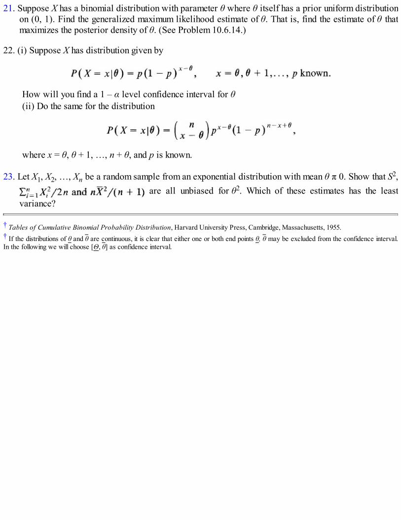
21. Suppose X has a binomial distribution with parameter θ where θ itself has a prior uniform distributionon (0, 1). Find the generalized maximum likelihood estimate of θ. That is, find the estimate of θ thatmaximizes the posterior density of θ. (See Problem 10.6.14.)

22. (i) Suppose X has distribution given by

How will you find a 1 – α level confidence interval for θ(ii) Do the same for the distribution

where x = θ, θ + 1, …, n + θ, and p is known.

23. Let X1, X2, …, Xn be a random sample from an exponential distribution with mean θ π 0. Show that S2, are all unbiased for θ2. Which of these estimates has the least

variance?

† Tables of Cumulative Binomial Probability Distribution, Harvard University Press, Cambridge, Massachusetts, 1955.† If the distributions of θ and θ are continuous, it is clear that either one or both end points θ, θ may be excluded from the confidence interval.In the following we will choose [Θ, θ] as confidence interval.

CHAPTER 11

Testing Hypotheses

11.1 INTRODUCTION

The basic ideas of hypothesis testing were first introduced in Section 4.4, where for the most part weconsidered samples of size 1 or 2 to avoid computational difficulties. In Chapters 6 and 8, however, weconsidered several important and widely applicable tests. In Chapter 9 we considered some large-sampletests that were based on the assumption that the test statistic has a limiting normal distribution. Indeveloping these tests, however, we mostly relied on our intuition: if large (small) values of the teststatistic supported the alternative hypothesis, we rejected H0 if the observed value of the test statistic islarge (small). Although we often made power computations we did not show (except in some examples ofSection 4.4) that the resulting procedure maximized the power function. In Section 11.2 we prove theNeyman–Pearson lemma, which gives the general procedure of constructing best (most powerful) tests inthe case when a simple null hypothesis is tested against a simple alternative hypothesis. In Section 11.3we show how the methods of Section 11.2 can sometimes be extended to yield best tests in morecomplicated situations.

A general method of constructing tests, especially when two or more unknown parameters areinvolved even though we may only be interested in testing for one of them, is given in Section 11.4. Thisso-called likelihood ratio test often yields reasonable results.

In Sections 11.5 through 11.9 we consider some nonparametric alternatives of tests introduced inearlier chapters. In Section 11.5 we consider the signed rank test, which may be used as an alternative tothe one sample t-test of Section 8.7. The two sample tests of Section 11.6 may be used as alternatives tothe two sample t-tests of Section 8.7. In Sections 11.7 and 11.8 we return to the problem of goodness offit considered earlier in Sections 4.5 and 9.9. In Section 11.9 we develop two procedures to test the nullhypothesis that no association exists between two variables against the alternative that a direct or indirectassociation exists.

11.2 NEYMAN–PEARSON LEMMA

In this section we concentrate on the case when Θ, the parameter set, contains only two values θ0 and θ1Let H0 the null hypothesis, be that X has distribution Pθ0

and let H1 be that X has distribution Pθ1. Both null

and alternative hypotheses are simple hypotheses so that the distribution of X is completely specifiedunder H0 as well as H1. Our object is to find a critical region C( X1,…, Xn) based on the sample X1, X2,…, Xn such that it has maximum power (or equivalently, the smallest type II error probability) at θ = θ1.We recall that the power function of any critical region is defined by

The following result due to Neyman and Pearson gives a complete solution to the problem.

THEOREM 1. (NEYMAN–PEARSON LEMMA). Let X1, X2,…,Xn be a random sample from adistribution with probability or density function f(x; θ). Suppose Θ = {θ0, θ1} and f(x; θ0) = f0(x) , f(x;θ1) = f1(x). Let

be the likelihood function of the sample. Then any critical region C of the form

for some 0 ≤ k < ∞ is best of its size for testing H0 : θ = θ0 against H1 : θ = θ1. For k = ∞, the criticalregion

is best of size zero for testing H0 against H1. (“Best” means the critical region has maximum power atθ = θ1.)

Proof. We note that for 0 ≤ k < ∞ the size of C in the continuous case is given by

Let C′ be any critical region such that its level is at most Pθ0(C). That is, let

Now (see Figure 1)

Figure 1

and

so that

and

Here we have written for convenience

Subtracting (3) from (2) we have

Next we note that for (x1,…, xn) ∈ C′ ∩ ⊆ , L(θ1) < kL(θ0) and for (x1,…, xn) ∈ C ∩ ′ ⊆ C,L(θ1) ≥ kL(θ0). It follows from (4) that

A similar argument applies in the discrete case.For the case k = ∞ we have Pθ0

(C0) = 0 so that C0 has size zero. Moreover, if critical region haslevel zero then Pθ0

( ) = 0 and ⊆ C0. (If contains any points (x1, x2,…, xn) for which L(θ0) > 0,then Pθ0

( ) cannot be zero.) Hence

Example 1. Number of System Failures. Suppose the number of system failures each month has a Poisson distribution withparameter λ. The number of such failures was observed for 12 months in order to test H0 : λ = 2 against : H1 : λ = 3. The likelihoodfunction is given by

and

The Neyman–Pearson critical region is of the form

Note, however, that L(3)/L(2) is an increasing function of , so that L(3)/L(2) ≥ k if and only if ≥ k ′ for some constantk ′≥ 0 (see Figure 2). Thus the critical region C0 = {(x1,…, xn) : ≥ k ′} is the best critical region of its size Pλ = 2(C0) for testingH0 : λ = 2 against H1 : λ = 3. Since has a Poisson distribution with parameter 12λ0 = 24 (under H0), we can compute the sizefor any given k ′. If, however, α, 0 < α < 1, is given as the level of significance we choose k ′ to be the smallest integer such that

Figure 2

Example 2. A Case Where X Has Continuous Density. Let X have density function

where θ ∈ [0, 1]. Suppose it is known that θ is either θ0 or θ1. The object is to choose between f(x; θ0) and f(x; θ1) based on a single

observation. We have

For definiteness, let θ0 < θ1. Let us examine L(θ1)/L(θ0) as a function of x. Set λ(x) = L(θ1)/L(θ0). Then

and it follows that λ(x) is an increasing function of x. Hence

so that

It is instructive to compare the graphs of L(θ0) and L(θ1) as done in Figure 3. Since large values of X are more probable under H1than under H0, the method of analysis we used in Section 4.4 also leads to the critical region C.

Given k ′ it is easy to compute the size of C and its power at θ1. Indeed,

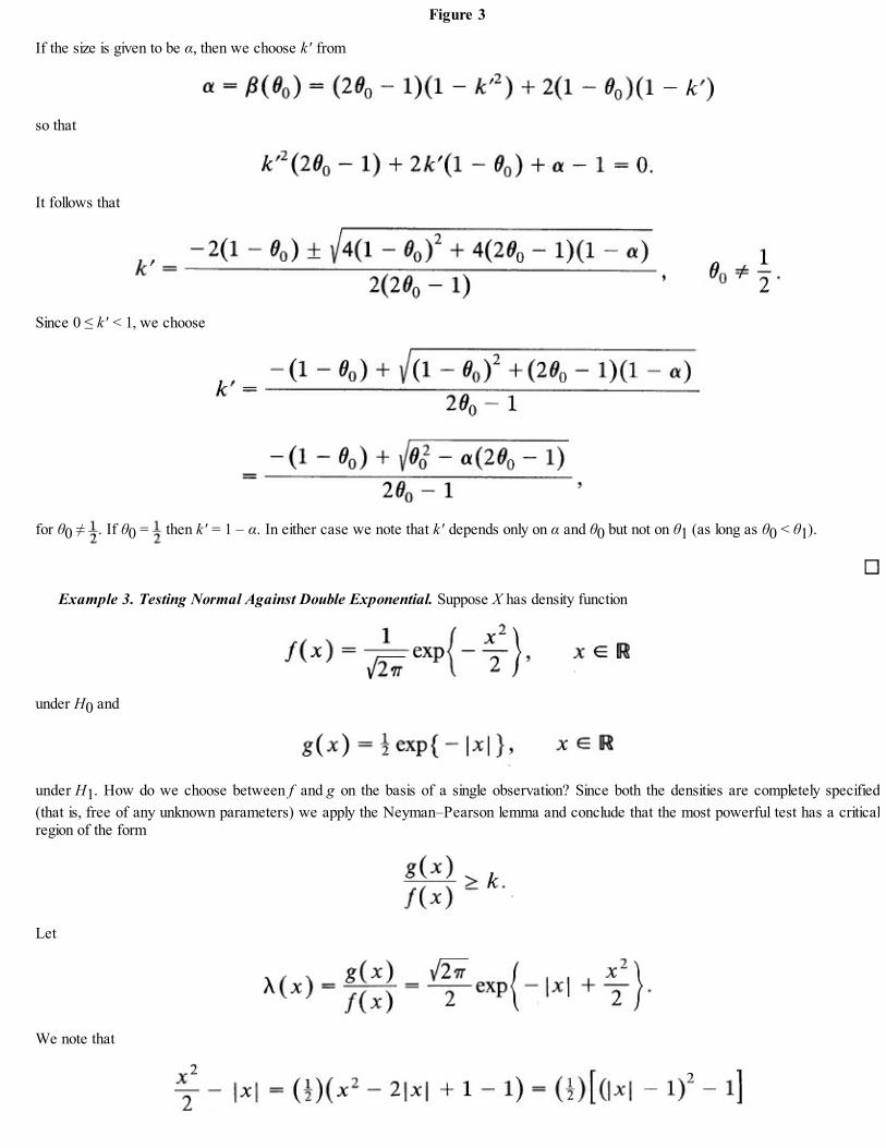
Figure 3

If the size is given to be α, then we choose k ′ from

so that

It follows that

Since 0 ≤ k ′ < 1, we choose

for θ0 ≠ . If θ0 = then k ′ = 1 – α. In either case we note that k ′ depends only on α and θ0 but not on θ1 (as long as θ0 < θ1).

Example 3. Testing Normal Against Double Exponential. Suppose X has density function

under H0 and

under H1. How do we choose between f and g on the basis of a single observation? Since both the densities are completely specified(that is, free of any unknown parameters) we apply the Neyman–Pearson lemma and conclude that the most powerful test has a criticalregion of the form

Let

We note that

so that

which is an increasing function of ||x|| – 1|. Hence

and it follows that C is of the form C = {x : |x| ≥ k1 or |x| ≤ k2} (see Figure 4). Thus if either a very large or a very small value of X isobserved, we suspect that H1 is true rather than H0. This is consistent with the fact that g has more probability in its tails and near zerothan f has. The size of C is given by

Figure 4. Graphs of f and g.

where Z has a standard normal distribution. The power of C is given by

Problems for Section 11.2

Find the Neyman–Pearson most powerful test of its size in Problems 1–10. Assume that a random sampleof size n is given. Simplify the test procedure as much as possible.

1. Let X have probability function P(X = 1) = θ = 1 – P(X = 0), 0 < θ < 1. Take H0 : θ = θ0 and H1 : θ =θ1 where θ1 > θ0.

2. Let X have probability function P(X = x) = θ(1 – θ)x–1, x = 1, 2,…, and zero elsewhere, 0 < θ 1. Take

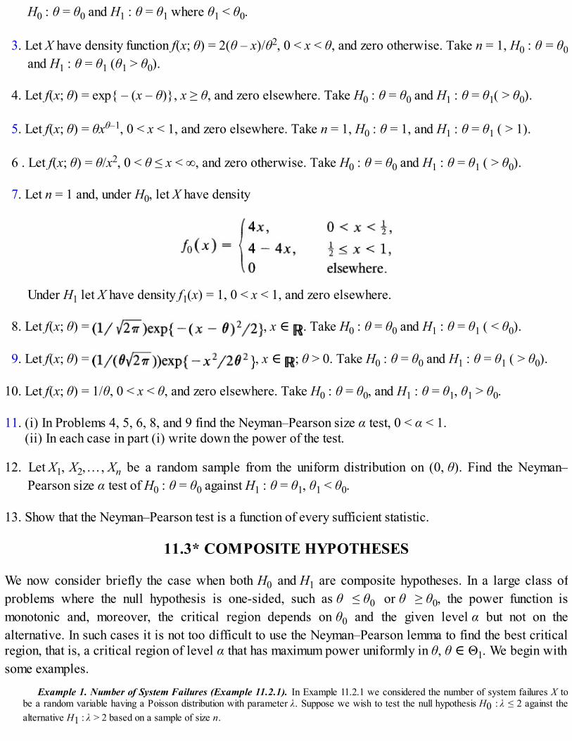
H0 : θ = θ0 and H1 : θ = θ1 where θ1 < θ0.

3. Let X have density function f(x; θ) = 2(θ – x)/θ2, 0 < x < θ, and zero otherwise. Take n = 1, H0 : θ = θ0and H1 : θ = θ1 (θ1 > θ0).

4. Let f(x; θ) = exp{ – (x – θ)}, x ≥ θ, and zero elsewhere. Take H0 : θ = θ0 and H1 : θ = θ1( > θ0).

5. Let f(x; θ) = θxθ–1, 0 < x < 1, and zero elsewhere. Take n = 1, H0 : θ = 1, and H1 : θ = θ1 ( > 1).

6 . Let f(x; θ) = θ/x2, 0 < θ ≤ x < ∞, and zero otherwise. Take H0 : θ = θ0 and H1 : θ = θ1 ( > θ0).

7. Let n = 1 and, under H0, let X have density

Under H1 let X have density f1(x) = 1, 0 < x < 1, and zero elsewhere.

8. Let f(x; θ) = , x ∈ . Take H0 : θ = θ0 and H1 : θ = θ1 ( < θ0).

9. Let f(x; θ) = , x ∈ ; θ > 0. Take H0 : θ = θ0 and H1 : θ = θ1 ( > θ0).

10. Let f(x; θ) = 1/θ, 0 < x < θ, and zero elsewhere. Take H0 : θ = θ0, and H1 : θ = θ1, θ1 > θ0.

11. (i) In Problems 4, 5, 6, 8, and 9 find the Neyman–Pearson size α test, 0 < α < 1.(ii) In each case in part (i) write down the power of the test.

12. Let X1, X2,…, Xn be a random sample from the uniform distribution on (0, θ). Find the Neyman–Pearson size α test of H0 : θ = θ0 against H1 : θ = θ1, θ1 < θ0.

13. Show that the Neyman–Pearson test is a function of every sufficient statistic.

11.3* COMPOSITE HYPOTHESES

We now consider briefly the case when both H0 and H1 are composite hypotheses. In a large class ofproblems where the null hypothesis is one-sided, such as θ ≤ θ0 or θ ≥ θ0, the power function ismonotonic and, moreover, the critical region depends on θ0 and the given level α but not on thealternative. In such cases it is not too difficult to use the Neyman–Pearson lemma to find the best criticalregion, that is, a critical region of level α that has maximum power uniformly in θ, θ ∈ Θ1. We begin withsome examples.

Example 1. Number of System Failures (Example 11.2.1). In Example 11.2.1 we considered the number of system failures X tobe a random variable having a Poisson distribution with parameter λ. Suppose we wish to test the null hypothesis H0 : λ ≤ 2 against thealternative H1 : λ > 2 based on a sample of size n.

Let λ1( > 2) be fixed and consider the problem of testing against . By the Neyman–Pearsonlemma, proceeding exactly as in Example 11.2.1, we see that any critical region of the form

is a most powerful region of its size. The power function of C is given by

where Y has a gamma distribution with parameters α = k and β = 1. It follows that Pλ(C) is an increasing function of λ and

Choose k such that C has level α; that is, choose k to be the smallest integer such that

Then C is a most powerful critical region of its size for testing λ ≤ 2 against λ = λ1.Next we note that C depends only on α but not on λ1 as long as λ1 > 2. Thus, no matter what λ1 we choose, as long as λ1 > 2, the

same critical region has maximum power against λ1. It follows that C is uniformly most powerful for testing H0 : λ ≤ 2 against H1 : λ > 2.

Example 2. Radiation Level of Microwave Ovens. Let X1, X2,…, Xn be the radiation readings in a random sample of n microwave

ovens produced by a certain manufacturer. Suppose Xi has a normal distribution with mean μ and variance σ2 (known). Therecommended limit for this type of radiation exposure is μ0 (milliroentgens per hour). Do the microwave ovens produced by thismanufacturer meet the recommended limit?

We wish to test H0 : μ ≤ μ0 against H1 : μ > μ0. Let μ1( > μ0) be fixed and consider the problem of testing μ = μ0 against μ = μl. Bythe Neyman–Pearson lemma it is easy to see that a critical region of the form

is a most powerful region of its size with power function

This follows since has a normal distribution with mean n μ and variance n σ2. Now

so that Pμ(C) is an increasing function of μ. Thus

which is the size of C (for testing against ). Hence the same test is a most powerful test of its size fortesting H0 : μ ≤ μ0 against . Next note that C is independent of μ1 (as long as μ1 > μ0) so that no matter what μ1( > μ0)we choose C has maximum power against μ1. Consequently, the test with critical region C is uniformly most powerful of size Pμ0

(C) fortesting μ ≤ μ0 against μ > μ0.

Examples 1 and 2 are typical special cases of a general result that holds for a large family ofdistributions. Rather than specify this general family and study its properties, we use the arguments usedin these examples to prove the following two results.

THEOREM 1. Suppose the Neyman–Pearson test of its size for the simple null hypothesis H0 : θ =θ0 against alternative θ = θ1 does not depend on θ1 ∈ Θ1. Then this test is a uniformly most powerfultest of its size for testing H0 : θ = θ0 against H1 : θ ∈ Θ1.Proof. Let C be the critical region of the Neyman–Pearson test of H0 against θ = θ1 of size Pθ0

((X1, X2,…,Xn) ∈ C). Suppose C does not depend on θ1 ∈ Θ1. Then C is most powerful against every θ1 ∈ Θ1 andhence is a uniformly most powerful test of its size.

We can now extend Theorem 1 to the case when H0 is also composite, as follows.

THEOREM 2. Suppose we wish to test H0 : θ ∈ Θ0 against H1 : θ ∈ Θ1 where both Θ0 and Θ1 haveat least two elements. Suppose further that for some θ0 ∈ Θ0 there is a uniformly most powerful test ofits size for testing θ = θ0 against θ ∈ Θ1 of the type described in Theorem 1. Let C be the criticalregion of this test. Consider the test with critical region C as a test of H0 vs. H1. If the level of this testof H0 is Pθ0

(C) (the size of C for testing θ = θ0 against θ ∈ Θ1) then C is a uniformly most powerful testof H0 against H1.

Proof. By hypothesis C is a uniformly most powerful size Pθ0(C) test of θ = θ0 against θ ∈ Θ1. Now any

test of H0 against H1 is also a test of θ = θ0 against θ ∈ Θ1. Since C is a level Pθ0(C) critical region of H0

against H1, it must be a uniformly most powerful level Pθ0(C) test of H0 versus H1.

Remark 1. It follows from Theorem 1 that if the Neyman–Pearson test of θ = θ0 against θ = θ1 dependson θ1, then there is no uniformly most powerful test of θ = θ0 against θ ∈ Θ1. In particular, this means thata uniformly most powerful test of θ = θ0 against θ ≠ θ0 usually does not exist. For instance, in Example 1there does not exist a uniformly most powerful test of λ = 2 vs. λ ≠ 2. This is essentially because there aretwo distinct best tests, one for λ = 2 vs. λ < 2 and one for λ = 2 vs. λ > 2.

Example 3. Testing σ2 ≥ vs. σ2 < . Let X1, X2,…, Xn be a random sample from a normal population with mean 0 and

variance σ2. Suppose we wish to test H0 : σ2 ≥ against H1 : σ2 < . Let σ1 < σ0 and consider the Neyman–Pearson test of vs.

with critical region

and size

We show that C is of level for testing H0 against H1. We note that has a chi-square distribution with n d.f.

when σ2 is the true variance. Thus

where Yn is a chi-square random variable with n d.f. Moreover for σ > σ0 we have

In view of Theorem 2 it follows that the test with critical region C is a size test of H0 against H1.

Problems for Section 11.3

1. (i) A coin is tossed n times in order to test if it is loaded in favor of heads. Find a uniformly mostpowerful test.

(ii) In particular, let n = 25 and suppose 17 heads are observed. Would you reject H0 : p = 1/2 infavor of H1 : p > 1/2 at level .10?

2. Let X be the lifetime of a light bulb manufactured by a certain company. Suppose X has densityfunction

Find a uniformly most powerful test of H0 : λ ≤ λ0 against H1 : λ > λ0.

3. The length of service of a component can be modeled by density function

Find a uniformly most powerful critical region for testing H0 : β ≤ β0 against β > β0 based on asample of n observations.

4. The number of accidents per week in a plant may be modeled by a Poisson random variable withmean λ where λ ≥ 4. A number of steps were taken to increase safety and hence reduce the averagenumber of accidents. After the campaign, an eight-week interval produced an average of threeaccidents per week. Construct a uniformly most powerful test of λ ≥ 4. Is there a significantimprovement at level α = .05?

5. Let X1, X2,…, Xn be the number of trials necessary to obtain the first success in n independentsequences of tosses of the same coin. The object is to test if the coin is fair against the alternative thatit is loaded in favor of heads. Find a uniformly most powerful test of H0 : p ≤ 1/2 where p is theprobability of a success.

6. From a group of N 18-year-old boys a sample of size n showed that x have registered for the draft.Find a uniformly most powerful test of H0 : D ≤ D0 against H1 : D > D0 where D is the total numberof boys in the group who have registered for the draft. If N = 1000, n = 25, and D0 = 500, howsignificant is the observed value x = 15?

7. Let X1, X2,…, Xn be a random sample from the following distributions. In each case find a uniformlymost powerful test of its size for testing H0 : θ ≤ θ0 against H1 : θ > θ0.

(i) f(x) = (1/θ)xθ–1, 0 < x < 1, and zero otherwise; θ > 0.(ii) f(x) = (1/Γ(θ))xθ–1e–x, x > 0, and zero otherwise; θ > 0.(iii)* f(x) = exp( – x + θ), x > θ, and zero elsewhere.

8*. Let X1, X2,…, Xn be a random sample from a uniform distribution on (0, θ). Find a uniformly mostpowerful test of

(i) H0 : θ ≤ θ0 against H1 : θ > θ0.(ii) H0 : θ ≥ θ0 against H1 : θ < θ0.

11.4* LIKELIHOOD RATIO TESTS

We now consider a general procedure based on an analysis of the likelihood function, which frequentlyleads to good test procedures when Θ1 has more than one point (that is, when H1 is composite).Moreover, the resulting test statistic has some desirable large-sample properties.

Let Θ ⊆ and let (X1, X2,…, Xn) be a random vector with probability or density function fθ, θ ∈ Θ.Consider the problem of testing the null hypothesis H0 : (X1, X2,…, Xn) has distribution fθ, θ ∈ Θ0 againstthe alternative H1 : (X1, X2,…, Xn) has distribution fθ, θ ∈ Θ1.

DEFINITION 1. (LIKELIHOOD RATIO). The likelihood ratio for testing H0 : θ ∈ Θ0 is defined to bethe ratio

The numerator of the likelihood ratio is the best explanation of the observation (x1, x2,…, xn) in the

sense of maximum likelihood estimation that the null hypothesis provides. The denominator is the bestpossible explanation of the observation (under the model). Intuitively we should reject H0 if there is abetter explanation of (x1, x2,…, xn) than the best one provided by H0. Clearly 0 ≤ λ(x1, x2,…,xn) ≤ 1.

DEFINITION 2. (LIKELIHOOD RATIO TEST). The likelihood ratio test for testing H0 : θ ∈ Θ0against H1 : θ ∈ Θ1 rejects H0 if λ(x1, x2,…, xn) < c for some constant c; 0 < c < 1.

The constant c is determined from the size α, 0 < α < 1, according to the relation

If no such c exists then we choose the largest c such that

Example 1. Testing for p in Sampling from a Bernoulli Distribution. Let X1, X2,…, Xn be a random sample from a Bernoullidistribution with parameter p, 0 ≤ p ≤ 1. We seek a level α likelihood ratio test of H0 : p ≤ p0 against H1 : p > p0. The likelihood functionis given by

where x1, x2,…, xn ∈ {0, 1}. Let s = be the number of 1’s in the sample. Now

since the maximum likelihood estimate of p is = s/n. We note that

so that L′(p) > 0 for p < s/n and L′(p) < 0 for p > s/n. Thus L(p) first increases, achieves its maximum at s/n, and finally decreases. Itfollows (see Figure 1) that

Consequently,

Figure 1. L(p) = ps(1 – p)n – s.

Since λ(s) ≤ 1 for np0 < s and λ(s) = 1 for s ≤ np0, λ(s) is a decreasing function of s. Thus

and the likelihood ratio test rejects H0 if s > c′, that is, if the number of 1’s in the sample is large. Here c′ > 0 is some constant (integer).We note that S has a binomial distribution with parameters n and p. The power function of the likelihood ratio test, given by

is a nondecreasing function of p (Example 7.5.2) so that

If the level α, 0 < α < 1, is preassigned then we choose c′ from

Often no such c′ exists because S has a discrete distribution. In that case we choose an integer c′ such that

Example 2. Student’s t-test as a Likelihood Ratio Test. Let X1, X2,…, Xn be a random sample from a normal distribution with

mean μ and variance σ2, both unknown. Suppose we wish to test H0 : μ = μ0 against H1 : μ ≠ μ0. Here Θ0 = {(μ0, σ2), σ2 > 0}, Θ1 =

{(μ, σ2) : μ ∈ , σ2 > 0} are both composite. The likelihood function of a sample of size n is given by

Since

are the unrestricted maximum likelihood estimates of μ and σ2 (see Example 10.5.4) respectively, we have, after some simplification,

Under H0, the maximum likelihood estimate of σ2 is easily shown to be

so that (after some simplification)

Hence

We note that λ(x1, … , xn) is a decreasing function of or of

. Hence

where s2 is the sample variance. We can rewrite the likelihood ratio test as

The statistic has a t-distribution with (n – 1) d.f. under H0 : μ = μ0 so that the likelihood ratio test is precisely the

two-tailed t-test. Given α, we choose c″ = tn–1, α/2.

Example 3. Testing for Independence of X and Y. Let (X1, Y1), (X2, Y2),…, (Xn, Yn) be a random sample from a bivariate normaldistribution with X1 = μ1, Y1 = μ2, var(X1) = , var(Y1) = , and ρ(X1, Y1) = ρ. We recall that X and Y are independent if andonly if ρ = 0. Hence a test of independence of X and Y can be based on ρ. More precisely, we wish to test H0 : ρ = 0 against H1 : ρ ≠ 0,say. Then

and

The likelihood function is given by

where θ = (μ1, μ2, σ1, σ2, ρ). Under H0, ρ = 0 and the maximum likelihood estimates of μ1, μ2, , are given respectively by

It follows that

Under Θ, the (unrestricted) maximum likelihood estimates of μ1, μ2, σ1, σ2 are the same as under Θ0, whereas the maximum likelihoodestimate of ρ is the sample correlation coefficient = r given (Problem 10.5.13) by

It follows that

The likelihood ratio test therefore rejects H0 if

or, equivalently, if

The exact distribution of the statistic R under H0 is known but we will not derive it here. It should be mentioned that the statistic T definedby

has, under H0, Student’s t-distribution with n – 2 d.f. This fact may be used to compute c′ for a given α, or the P-value associated with anobserved value of R.

Remark 1. (Relation Between Likelihood Ratio Test and Neyman–Pearson Test) . Does thelikelihood ratio test of a simple null hypothesis against a simple alternative hypothesis coincide with theNeyman–Pearson test? The following result holds. Suppose the Neyman–Pearson and the likelihood ratiotests exist for a given size α. Then they are equivalent. We will not prove this result here.

Remark 2. (Large Sample Distribution of λ). In the examples considered above, the test statistic turnsout to have a well known distribution under H0. This, however, is not always the case. How then do wecompute the P-value or perform the test? The main advantage of the likelihood ratio test is that undercertain regularity conditions on the underlying distribution, the statistic – 2 ln λ(X1, X2,…, Xn) has, forlarge n, approximately a chi-square distribution under H0. The degrees of freedom equal the number ofunknown parameters under Θ minus the number of unknown parameters under Θ0. In Examples 1, 2, and 3the degree of freedom is 1. In Example 2,

has, for large n, approximately a chi-square distribution with 1 d.f. Hence the likelihood ratio test rejectsH0 if

or if

The approximate P-value is therefore given by

which is computed from χ2(1) tables. However, for large n, a t-statistic T is approximately normal so thatT2 is approximately χ2(1). Since

we have

so that the P-value is (approximately) the same whether we compute it under χ2(1) or under t-distribution.

Problems for Section 11.4

1. Let X1, X2,…, Xk be a sample from probability function

PN (X = j) = 1/N, j = 1, 2,…,N, N ≥ 1 is an integer, and zero otherwise.

(i) Find the likelihood ratio test of H0 : N ≤ N0 against H1 : N > N0.(ii) Find the likelihood ratio test of H0 : N = N0 against H1 : N ≠ N0.

2. Find the likelihood ratio test of θ = θ0 against θ ≠ θ0 based on a sample of size 1 from density function

3. Let X1, X2,…, Xn be a sample from density function

Find the likelihood ratio tests of(i) H0 : θ ≤ θ0 against : H1 : θ > θ0,(ii) H0 : θ = θ0 against H1 : θ ≠ θ0.

4. Let X1, X2,…, Xn be a random sample from a Poisson distribution with parameter λ > 0. Find thelikelihood ratio tests of

(i) H0 : λ = λ0 against H1 : λ ≠ λ0.(ii) H0 : |λ – λ0| ≤ a against H1 : |λ – λ0| > a where a is a known constant.

(iii) H0 : λ ≥ λ0 against H1 : λ < λ0.

5. Find the likelihood ratio test of H0 : p = p0 against p ≠ p0 based on a sample of size 1 from probabilityfunction

and zero otherwise, 0 ≤ p ≤ 1.

6. Let X1, X2,…, Xn be a sample from a normal distribution with unknown parameters μ and σ2. Find thelikelihood ratio tests of

(i) H0 : σ = σ0 against H1 : σ ≠ σ0,(ii) H0 : σ ≤ σ0 against H1 : σ > σ0.

7*. Let X1, X2,…, Xm and Y1, Y2,…, Yn be independent random samples from normal distributions withmeans μ1 and μ2, and variances and respectively. Find the likelihood ratio tests of

(i) H0 : = σ1 = σ2 against H1 : σ1 ≠ σ2 (μ1, μ2 both unknown).(ii) H0 : μ1 = μ2 against H1 : μ1 ≠ μ2 (σ1, σ2 unknown but equal).

8. Let X1, X2,…,Xm and Y1, Y2,…, Yn be independent random samples. Suppose the X’s have commondensity

and the Y’s have common density

Find the likelihood ratio test of H0 : = λ1 = λ2 against H1 : λ1 ≠ λ2.

9. Let (X1, X2,…, Xk–1) be one observation from multinomial distribution

where xk = n – , 0 ≤ xi, ≤ n, 0 ≤ pi ≤ 1, . Find the likelihood ratio test of H0 : p1 =p2 = ··· = pk = 1/k against H1 that at least one inequality holds in p1 = p2 = ··· = pk.

10*. Let X11, X12,…, X1n1, X21, X22,…, X2n2

, and X31, X32,…, X3n3 be independent random samples from

normal distributions with unknown means μ1, μ2, μ3 and unknown variances , , respectively.Find the likelihood ratio tests of

(i) H0 : σ1 = σ2 = σ3 against the alternative that there is at least one inequality.(ii) H0 : μ1 = μ2 = μ3 against the alternative that there is at least one inequality, assuming that μ1 = μ2

= μ3 but the common value is unknown.

11. Show that the likelihood ratio test statistic is a function of every sufficient statistic.

11.5 THE WILCOXON SIGNED RANK TEST

In Section 6.3.3 we discussed the sign test as a test of median or for comparing two populations based onpaired observations. We recall that the sign test is rather crude in that it uses only the sign of thedifference between each observation and the postulated value of the median but ignores the magnitude ofthese differences. Often the magnitude of these differences are also available. The Wilcoxon signed ranktest that we now study uses both the sign and the magnitude of the differences.

Let X1, X2,…, Xn be a random sample from a continuous symmetric distribution. Let = med(X) andsuppose we wish to test the null hypothesis H0 : = against the alternative H1 : > . Consider thedifferences X1 – , X2 – ,…, Xn – . Clearly, under H0, Xi – has a continuous symmetricdistribution about zero. Consequently, under H0, we expect negative and positive differences to be aboutevenly spread out. That is, the expected number of negative differences is n/2 and, moreover, negativeand positive differences of equal absolute magnitude should occur with equal probability.

For convenience, set Di = Xi – . Since the Xi’s have a continuous distribution P(Di = 0) = 0 and weassume that |Di| > 0 for i = 1, 2,…, n and Di ≠ Dj for i ≠ j. Consider the absolute values |D1|, |D2|,…, |Dn|and rank them from 1 (for the smallest) to n (for the largest). Let W+ be the sum of ranks assigned to thoseDi’s that are positive and W– be the sum of ranks assigned to Di’s that are negative. Clearly,

so that W+ and W– offer equivalent test statistics. Under H0 we expect W+ and W– to be the same. Since alarge of value of W+ indicates that most of the larger ranks are assigned to positive Di’s, it follows thatlarge values of W+ support H1 : > . In view of relation (1) it is sufficient to compute the smaller ofW+ and W– and then compute the larger value by differencing. The same argument applies to thealternative H1 : < or H1 : ≠ . Let w0 be the observed value of W+ (or W–).

Even though we assume that the distribution is continuous, ties and zeros do occur in practice. As inthe case of a sign test, the recommended procedure is to drop the zeros and use the reduced sample size. Ifthere are ties, that is, if some of the Di’s are equal, assign to each such Di a rank equal to the simplearithmetic average of the ranks these Di’s would have received if they were not equal. Thus the ordered

observations 2, 2, 5, 5, 7, 8, 8, 8, 10, 11 are assigned, respectively, the ranks 1.5, 1.5, 3.5, 3.5, 5, 7, 7, 7,9, 10.

Table A11 in the Appendix gives the cumulative right tail probabilities PH0(W ≥ w0) for values of w0

≥ n(n + 1)/4 and n = 2, 3,…, 15. (Here W is interpreted as either W+ or W–.) For larger values of n weuse the normal approximation. Under H0, the common distribution of W+ and W– is symmetric about themean

with variance

and the standardized W+ has approximately a standard normal distribution. Thus

Example 1. Pulse Rate of Infants Aged One Month or Over. A random sample of 15 infants one month or older shows thefollowing pulse rates (beats per minute):

Assuming that the distribution of pulse rates is symmetric and continuous, is there evidence to suggest that the median pulse rate of onemonth or older infants is different from 120 beats per minute?

We wish to test H0 : = 120 against H1 : , ≠ 120. Let us compute Di = Xi, – = Xi – 120, |Di| and rank of |Di|.

Excluding the two 0’s we arrange the observations in increasing order as

with ranks

Hence

so that

For the reduced sample size n = 13, PH0(W+ ≥ w0) = .153 so that the associated P-value is 2(.153) = .306. Thus, under H0 the chance of

observing as large a value of W+ as 61 is 30.6 percent and we can hardly reject H0.Let us analyze the data using the sign test. The number of negative signs is 5 so that the P-value under H0 : p = 1/2 is

The sign test is more conservative.If we assume that the distribution of pulse rates is normal, then we can test H0 : μ = 120 against H1 : μ ≠ 120 using a two-tailed t-test.

We have

so that

For 14 d.f.

so that the P-value is about .30, which is approximately the same as that obtained by the Wilcoxon signed rank test. In general, the signtest performs worse than the t- and signed rank tests, at least for large samples. For large samples, the signed-rank test performsrelatively well in comparison with the t-test (even when the underlying distribution is normal). For small samples from nonnormalpopulations, either the sign test or signed rank test may be more powerful than the t-test. The sign-ranked test should be preferable to thesign test in situations when the underlying distribution is symmetric.

Remark 1. The Wilcoxon signed rank test can also be used as a test for symmetry. Suppose x1, x2,…,xn is a random sample from a continuous population with median . Then we can test either

or

by using W+ or W– exactly as described above.

Remark 2. The same test can be used for paired data (X1, Y1),(X2, Y2),…, (Xn, Yn) to test H0 :median(Xi – Yi) = against one-sided or two-sided alternatives. In this case we assume that Xi – Yi have acontinuous and symmetric distribution about their median . The test is performed exactly as above bytaking Di = |Xi – Yi – |. The case of most interest is when = 0.

Example 2. Effect of Smoking on Pulse Rate. In order to determine if smoking results in increased heart activity a random sampleof 20 people was taken. Their pulse rates (beats per minute) before smoking and after smoking a certain brand of cigarette are measuredwith the following results:

We wish to test H0 : = 0 against H1 : < 0 where Di = Xi – Yi, i = 1, 2,…, n. Assuming that Di, have a continuous symmetricdistribution we can test H0 by using Wilcoxon signed rank test. Ignoring the three observations where xi = yi and arranging |di| inincreasing order of magnitude, we have

Thus

so that

Since n > 15, we use normal approximation. We have

Hence

so that w– = 138 is highly significant and it is reasonable to conclude that smoking does increase the pulse rate.For comparative purposes let us also apply the sign test. The number of negative signs S is 14. Under H0, p = 1/2 and under H1 : p >

1/2 where p = P(X1 < Yi). Thus the associated P-value is

and we reject H0 at level α ≥ .0064. We leave the reader to show that the t-test also results in rejection of H0 with P-value < .005.

Problems for Section 11.5

1. A certain university’s brochure claims that the average amount of money needed for boarding andlodging in the town for a single student is $75 per week. A random sample of nine single students fromthis university showed the following weekly expenditures:

Is there evidence to suggest that the university’s estimate is not correct? Assuming that the weeklyexpenditures are normally distributed, also apply the t-test to analyze the same data.

2. Assume that the average birth weight of infants is known to be 7 pounds. The birth weights of a randomsample of 11 children born to migrant workers were recorded (in pounds) as follows:

Is it reasonable to conclude that the average birth weight of children of migrant workers is smaller thanthe national average? Analyze the same data by performing the t-test and the sign test.

3. In order to keep track of inflation, a Network News Program visits 10 selected supermarkets on thefirst Monday of every month and buys a typical market basket of 30 preselected items. The total costdata for November 1, 1982, and November 7, 1983, were as follows:

Is there evidence to suggest that the average market cost remained the same over the 12-monthperiod? Analyze the same data by using a t-test.

4. In order to determine if children watch more TV in preteen years, a random sample of 20 children agednine, ten, or eleven was selected and their daily average TV viewing times were recorded. The samechildren were then canvassed four years later and their daily average viewing time was recorded.

How strong is the evidence that the TV watching habits in preteen and teen years is the same?

5. A group of 10 students is given a task to perform while sober. Each student is then given three beersover a one-hour period and asked to repeat the task. The results are as follows:

How strong is the evidence that alcohol dulls mental ability?

6. In order to compare the effectiveness of two sunburn lotions, a random sample of seven subjects isselected. Lotion A is applied to the left side of their faces and Lotion B to the right side. After thesubjects have sat in the sun watching a three-hour tennis match, the degree of sunburn is measured on ascale.

Do the data support the claim that the two lotions are equally effective?

7. The following observations were taken from a table of random numbers from a distribution F withmedian 0.

Is it reasonable to conclude that F is a symmetric distribution?

8. The median time for a tune-up of a four-cylinder car is known to be 45 minutes. A random sample of 12mechanics showed tune-up times, in minutes, of

What conclusion do you draw from the sample?

9. Consider the density function

and 0 elsewhere.(i) Graph g.(ii) Show that h defined by h(X) = if X < 1/2, = if X > 1/2,

where X is the uniform distribution on (0, 1) has density g(y).(iii) Use part (ii) to generate a sample of size 20 from density g with θ = 1 given a random sample of

size 20 from a uniform distribution on (0, 1):

(iv) Use the sample in part (iii) to test H0 : median of g = ζ.5(g) = 1 against H1 : ζ.5(g) ≠ 1. Comparethe performance of sign, Wilcoxon signed rank, and t-tests.

11.6 SOME TWO-SAMPLE TESTS

The sign and the Wilcoxon signed rank tests are one-sample tests that are the nonparametric analogs of theone-sample t-test based on normal theory. We now consider some nonparametric analogs of the two-sample t-test. Recall that if X1, X2,…, Xm and Y1, Y2,…, Yn are independent random samples from twonormal populations with common (unknown) variance, then the t-statistic defined by

where

and

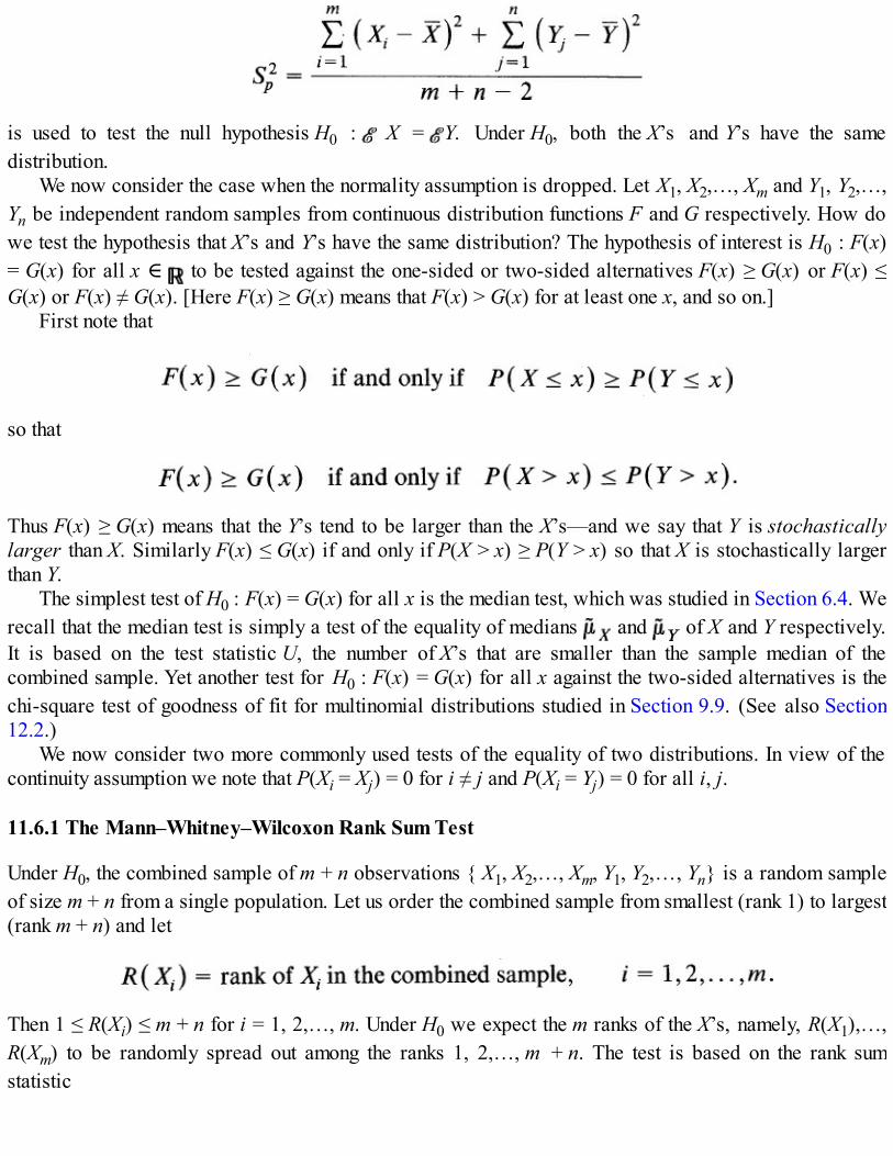
is used to test the null hypothesis H0 : X = Y. Under H0, both the X’s and Y’s have the samedistribution.

We now consider the case when the normality assumption is dropped. Let X1, X2,…, Xm and Y1, Y2,…,Yn be independent random samples from continuous distribution functions F and G respectively. How dowe test the hypothesis that X’s and Y’s have the same distribution? The hypothesis of interest is H0 : F(x)= G(x) for all x ∈ to be tested against the one-sided or two-sided alternatives F(x) ≥ G(x) or F(x) ≤G(x) or F(x) ≠ G(x). [Here F(x) ≥ G(x) means that F(x) > G(x) for at least one x, and so on.]

First note that

so that

Thus F(x) ≥ G(x) means that the Y’s tend to be larger than the X’s—and we say that Y is stochasticallylarger than X. Similarly F(x) ≤ G(x) if and only if P(X > x) ≥ P(Y > x) so that X is stochastically largerthan Y.

The simplest test of H0 : F(x) = G(x) for all x is the median test, which was studied in Section 6.4. Werecall that the median test is simply a test of the equality of medians and of X and Y respectively.It is based on the test statistic U, the number of X’s that are smaller than the sample median of thecombined sample. Yet another test for H0 : F(x) = G(x) for all x against the two-sided alternatives is thechi-square test of goodness of fit for multinomial distributions studied in Section 9.9. (See also Section12.2.)

We now consider two more commonly used tests of the equality of two distributions. In view of thecontinuity assumption we note that P(Xi = Xj) = 0 for i ≠ j and P(Xi = Yj) = 0 for all i, j.

11.6.1 The Mann–Whitney–Wilcoxon Rank Sum Test

Under H0, the combined sample of m + n observations { X1, X2,…, Xm, Y1, Y2,…, Yn} is a random sampleof size m + n from a single population. Let us order the combined sample from smallest (rank 1) to largest(rank m + n) and let

Then 1 ≤ R(Xi) ≤ m + n for i = 1, 2,…, m. Under H0 we expect the m ranks of the X’s, namely, R(X1),…,R(Xm) to be randomly spread out among the ranks 1, 2,…, m + n. The test is based on the rank sumstatistic

Under H0 we expect TX to be proportional to the sample size m. A very large value of TX indicates that theX’s tends to be larger than the Y’s so that a large value of TX supports the alternative H1 : F(x) ≤ G(x).Similarly, a very small value of TX supports the alternative H1 : F(x) ≥ G(x).

We note that

so that TX and TY offer equivalent test statistics. Although ties are theoretically impossible, they do occurin practice. In case of ties we assign average rank to the tied observations (as in Section 11.5). In thefollowing test, tx is the observed value of TX.

Often the test is stated in terms of the statistic UX where

Since, however,

we have

It follows that

and UX and TX are equivalent test statistics.In order to compute the P-value (or to find the critical region if α is given), one needs the null

distribution of TX. Table A10 in the Appendix gives the cumulative probability in the tail of TX. Sincelabeling of X and Y can be interchanged, we assume that the sample with fewer observations is the Xsample so that m ≤ n. Next note that the least value of TX corresponds to the ranks 1, 2,…, m and themaximum value corresponds to ranks n + 1, n + 2,…, n + m. It follows that

Finally, under H0, TX has a symmetric distribution about its mean m(m + n + 1)/2. It follows that a left tailcumulative probability equals the corresponding right tail cumulative probability. Table A10 gives theright tail probabilities for TX ≥ m(m + n + 1)/2 for values of m ≤ n ≤ 10. Left tail probabilities areobtained by symmetry. Indeed, if tx ≤ m(m + n + 1)/2, then

Suppose, for example, that m = 5, n = 7, and tx = 18. Then tx = 18 < 5(5 + 7 + 1)/2 so that

For larger values of m or n we use the fact that

and

has approximately a standard normal distribution. Since TX is integer valued, the application of continuitycorrection (Section 9.4) results in an improved approximation.

Example 1. Comparing Two Methods of Instruction. Seventeen students were randomly selected to participate in an educationalresearch project. A group of eight students was asked to attend a traditional lecture course for four weeks. The remaining nine studentswere provided self-instructional material on video cassettes. At the end of four weeks all the students took the same test with thefollowing results.

At what level is the difference between the scores of the two groups significant?Here we wish to test H0 : F = G against the two-sided alternative H1 : F ≠ G. Let the lecture scores represent X-values and self-

instruction scores the Y-values, so that m = 8 and n = 9, m < n. Combining the scores, arranging them in increasing order, and assigningaverage rank to tied observations, we have:

It follows that

Since the mean value is 8(8 + 9 + 1)/2 = 72 we see that tx is in the right tail so that the P-value associated with TX = 83.5 is 2PH(TX ≥83.5). Table A10 only gives values of cumulative tail probability for integral values of tx. We note the

We estimate the right tail probability for 83.5 as the average (.161 + .138)/2, so that the P-value is .299. Since there is about a 30 percentchance of observing as large a value of TX as 83.5 in random sampling under H0, the data do not indicate a significant difference betweenthe two sets of scores.

Suppose, on the other hand, that the level of significance is given to be α = .10. In that case we wish to find the critical region TX ≥ c3or TX ≤ c4. By symmetry we need to find c such that

From Table A10, c = 90 = c3 and c4 = 54 since

Example 2. Comparing Failure Times of Two Types of Light Bulbs. The failure times of a certain type of light bulb manufacturedby two different companies, X and Y, are given (in hundreds of hours) below:

Let us test the null hypothesis of equality of two medians against a one-sided alternative H1 : > . Combining the two samples andarranging them in increasing order of magnitude, we have

Thus tx = 1 + 2 + 3 + 4 + 9 + 11 = 30 with P-value PH0(TX ≤ 30) = PH0

(TX ≥ 48) = .09. We conclude that the data do not substantiate

the claim that > at the 5 percent level but they do substantiate it at the 10 percent level.

Example 3. Breaking Strength of Two Types of Nylon Fiber. In order to compare the breaking strength of nylon fiber produced by

two different manufacturers, 10 measurements on one (say X) and 13 on the other (say Y) were taken with the following results.

Do the data indicate a significant difference between the breaking strengths?Here m = 10, n = 13 and we have to use the normal approximation. Let us first find the observed value of TX.

Thus tx = 1 + 2 + 3 + 4.5 + 7 + 10 + 10 + 13.5 + 16.5 + 19.5 = 87. We note that

and since tx < 120, the smaller tail probability is the left tail probability. Hence the P-value is given by

If we allow an error of no more than, say, .04 of rejecting a true null hypothesis, then we have to conclude that the brands of fiber havethe same distribution of breaking strength. If, on the other hand, α = .05, we will have to reject H0 : F = G.

11.6.2 The Runs Test

Consider an ordered sequence of two types of symbols. A run is a succession of one or more identicalsymbols which are preceded and followed by a different symbol (or no symbol). The length of a run isthe number of like symbols in a run.

Example 4. Sex of Newborns at a Hospital. The sexes of 15 children at a hospital are recorded in order of their birth with thefollowing results.

Here G stands for a girl and B for a boy. We underline groups of successive like symbols. Each underlined group is a run. Thus we havea run of length 2 (of G symbols), followed by a run of length 3 (of B symbols), and so on. The total number of runs in this sequence isseven.

The total number of runs can be used as a test statistic to test the equality of two distributions. Let X1,X2,…, Xm and Y1, Y2,…, Yn be independent random samples with respective continuous distributionfunctions F and G. Let us arrange the combined sample in increasing order of magnitude (and assume forthe moment that there are no ties between X and Y values). Replace the X-observations in this orderedarrangement by symbol x and the Y-observations by symbol y. Let R be the total number of runs in thisordered arrangement of m + n symbols of type x and y. (We assume for the moment that there are no tiesbetween x’s and y’s.)

Under H0 : F(x) = G(x) for all x, we expect the symbols x and y to be well-mixed. If, for example, thex’s tend to be larger than the y’s, then most of the y’s will precede the x’s and we will have fewer runs.The same argument applies to the case when y’s tend to be larger than the x’s. It follows that a small valueof R supports the alternative H1 : F(x) ≠ G(x). It is clear that a test based on R is appropriate only fortwo-sided alternatives.

In case of ties between x’s and y’s, a conservative procedure is to break the ties in all possible ways.For each such resolution of ties, compute the value of R. Then use the largest possible value of R to givethe largest P-value. For example, if one x and one y are tied there are two possible resolutions:

and

resulting in two values of R. Take the larger of the two R-values.In order to perform the test (or to compute the P-value), we need the null distribution of R. Table A12

in the Appendix gives the left tail cumulative probabilities for all values of m ≤ n with m + n ≤ 20. Forlarger values of m or n, we use the normal approximation. We have

and the statistic

has approximately a standard normal distribution. Since R is integer valued, continuity correction shouldbe applied to improve the normal approximation.

Example 5. Comparing Two Methods of Instruction (Example 1). We return to Example 1 where we used the Mann–Whitney–Wilcoxon test to compare two methods of instruction. We note that there is one tie between X and Y values at 78. Thus we have twoways of breaking the tie. Taking the X value corresponding to 78 first, we have

so that R = 10. Taking the Y value corresponding to 78 first, we have

so that R = 8. Thus we take the larger of the two values as the observed value of R. The P-value is therefore PH0(R ≤ 10). We note that

PH0(R ≤ 10) > .5, which is considerably larger than the P-value given by the Mann–Whitney–Wilcoxon test. In any case the data do

substantiate the null hypothesis that there is no difference between the two methods of instruction.

Example 6. A Comparison of the Performance of Some Two-Samples Tests. In order to compare the two-sample tests studied sofar, we take two independent random samples from normal populations with means 0 and 1 respectively.

Let us test the null hypothesis H0 : = , that the two samples have the same medians, against H1 : ≠ in order to seewhich test is best able to detect the difference between the means ( = medians).

t-test: We have = 4.32/9 = 0.48, = 12.24/9 = 1.36,

and

Hence

so that the P-value is slightly less than .05. (For 16 d.f. P(T ≤ – 2.12) = .025.)

Median test: We arrange the combined sample in increasing order, as shown.

Hence

(The sample median is any number between 1.022 and 1.179.) The smaller tail probability corresponds to PH0(U ≥ 6) so that the P-value

is

It is clear that the median test performs rather poorly.

Mann–Whitney–Wilcoxon Test. We note that

and since the mean value is 9(9 + 9 + 1)/2 = 85.5, the P-value is two times the probability PH0(TX ≤ 65). Thus

The Mann–Whitney–Wilcoxon test therefore rejects H0 at the 10 percent level but not at the 5 percent level and compares rather wellwith the t-test even though it does not use the assumption of normality required for the t-test.

Runs test. We note that R = 8 so that the P-value is PH0 (R ≤ 8) = .238. Thus the runs test performs better than the median test but

does much worse than the Mann–Whitney–Wilcoxon test.

A theoretical comparison of these two sample tests is beyond our scope. We state without proof that typically the runs test and themedian test perform rather poorly in comparison with the Mann–Whitney–Wilcoxon test, which typically performs almost as well as the t-test if the underlying distribution is normal. If the underlying distribution is not normal the Mann–Whitney–Wilcoxon test is considered tobe the best nonparametric test to detect shifts in location.

Remark 1. (The Runs Test for Randomness) . The statistic R is often used to test if an orderedsequence of two types of symbols is a random arrangement. If all possible distinguishable arrangementsof the two types of symbols have the same chance, we say that the arrangement is random. Suppose forexample that x1, x2,…, xm and y1, y2,…, yn are independent random samples from the same population.Then in the ordered arrangement of x and y symbols we expect the symbols to be randomly distributed.The alternative is usually taken to be two-sided, namely, that the sequence is nonrandom. If H0 is rejected,then either the two samples do not come from the same population or they are not independent. Under thenull hypothesis of randomness we expect the number of runs of the x symbols to be approximately thesame as those of y symbols. If R is too small or too large then the two types of symbols are eitherclustered together or isolated, indicating nonrandomness. Hence we reject H0 if R is either too large ortoo small.

Example 7. Tossing a Fair Coin. Students were asked to toss a fair coin 20 times and report the results to the instructor. A studentturned in the following sequence of heads (H) and tails (T):

Does this sequence of 10 heads and 10 tails indicate departure from randomness? In other words, is there evidence to conclude that thestudent in question did not conduct the experiment? We note that the number of runs is given by r = 15. From Table A12 for m = n = 10,

so that the P-value is 2(.051) = .102 and we cannot reject H0 at level α = .10. That is, there does not appear to be an intentional mixing ofsymbols on the part of the student.

Problems for Section 11.6

1. The order in which test questions are asked affects a student’s ability to answer them correctly andhence affects the student’s total grade. In order to check this proposition, two tests were made. Test Ahad questions set in increasing order of difficulty; in Test B the order was reversed. A randomsample of 20 students was selected in such a way that 10 pairs of students were matched in ability.From each pair, one student was assigned randomly to take Test A and the other Test B. Thefollowing scores were obtained.

Is there evidence to indicate that the scores on Test B are lower than those on Test A? Use bothMann–Whitney–Wilcoxon and t-tests.

2. In a controlled laboratory environment, eight men and 10 women were tested to determine the roomtemperatures they found to be most comfortable. The following results were obtained.

Assuming that these samples are random samples from their respective populations, is the averagecomfortable temperature for men lower than that for women?

3. Nineteen pieces of flint were collected, nine from area A and ten from area B. The object of the studywas to determine if the pieces of flint were of equal hardness. For the purposes of the study nineteenpieces of flint of equal hardness from a third area were brought in. Each of the sample pieces wasthen rubbed against a piece from the third area. The nineteen sample pieces were then orderedaccording to the amount of damage sustained from the softest (most damage) to the hardest (least

damage): A A B B A A B B B B A A B A A A B B B.Is there evidence to suggest that the flints from areas A and B are of equal hardness? Use both Mann–Whitney–Wilcoxon and runs tests to analyze the data.

4. Fifteen three-year-old boys and 15 three-year-old girls were observed during two 30-minute sessionsof recess in a nursery school. Each child’s play was scored for incidence and degree of aggression asfollows:

Is there evidence to suggest that there are sex differences in the incidence and amount of aggression?Use both Mann–Whitney–Wilcoxon and runs tests.

5. Two laboratory cultures are to be compared for difference in bacteria counts. Independent randomsamples of six from culture A and eight from culture B are taken and the number of bacteria per unitof volume are recorded as follows:

Is there evidence to conclude that the bacteria counts for the two populations are not the same?

6. A true–false examination with 50 questions has the following sequence of answers.

Is there evidence to suggest that the instructor used intentional mixing of answers?

7. Twenty-five items emerging from a production line are tested and classified as defective (D) ornondefective (N). The following sequence is obtained:

How strong is the evidence that there is lack of randomness in the sequence?

8. An intelligence test was administered to 10 men and 12 women with the following test scores:

Is it reasonable to conclude that there are no sex differences in average intelligence? Use the Mann–Whitney–Wilcoxon test as well as the t-test.

9. The following digits are chosen from Table A1, line 5.

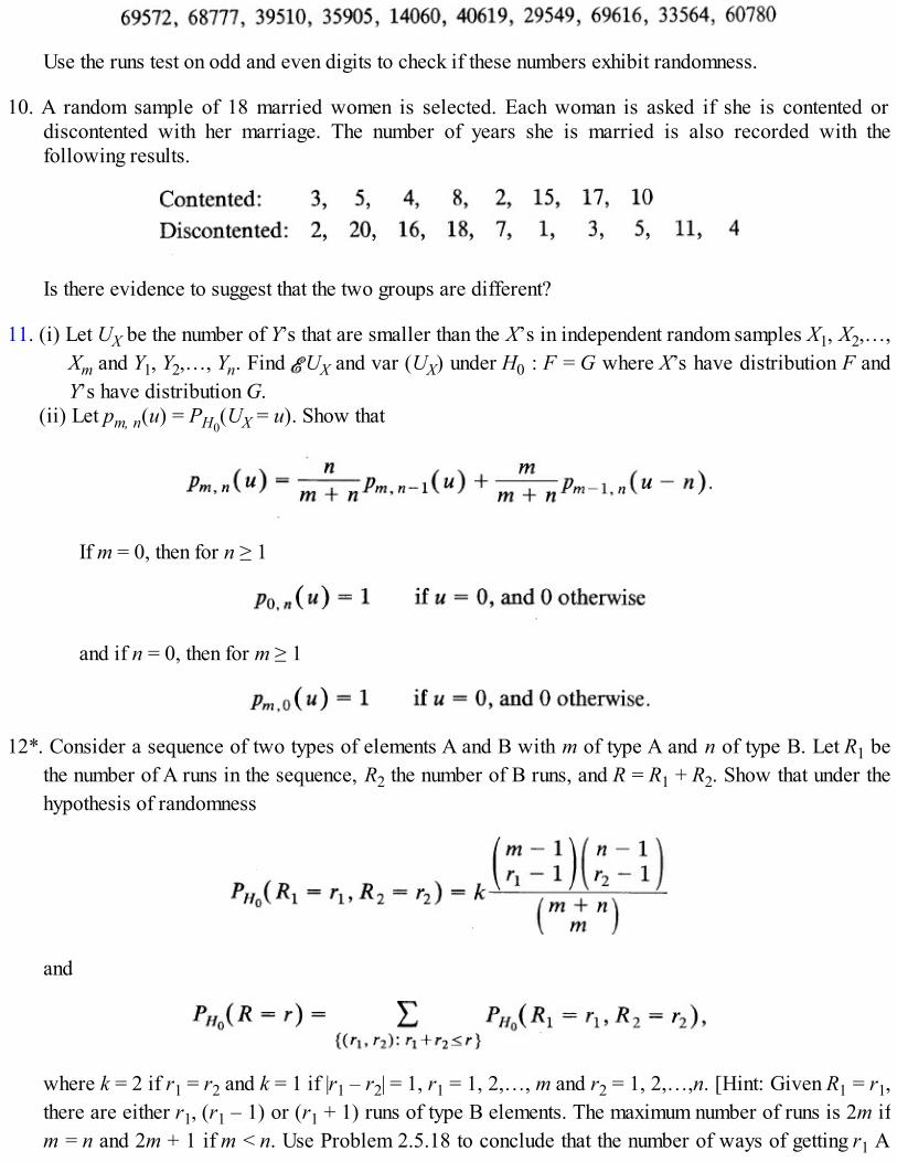
Use the runs test on odd and even digits to check if these numbers exhibit randomness.

10. A random sample of 18 married women is selected. Each woman is asked if she is contented ordiscontented with her marriage. The number of years she is married is also recorded with thefollowing results.

Is there evidence to suggest that the two groups are different?

11. (i) Let UX be the number of Y’s that are smaller than the X’s in independent random samples X1, X2,…,Xm and Y1, Y2,…, Yn. Find UX and var (UX) under H0 : F = G where X’s have distribution F andY’s have distribution G.

(ii) Let pm, n(u) = PH0(UX = u). Show that

If m = 0, then for n ≥ 1

and if n = 0, then for m ≥ 1

12*. Consider a sequence of two types of elements A and B with m of type A and n of type B. Let R1 bethe number of A runs in the sequence, R2 the number of B runs, and R = R1 + R2. Show that under thehypothesis of randomness

and

where k = 2 if r1 = r2 and k = 1 if |r1 – r2| = 1, r1 = 1, 2,…, m and r2 = 1, 2,…,n. [Hint: Given R1 = r1,there are either r1, (r1 – 1) or (r1 + 1) runs of type B elements. The maximum number of runs is 2m ifm = n and 2m + 1 if m < n. Use Problem 2.5.18 to conclude that the number of ways of getting r1 A

runs is

13. Show that the marginal distribution of R1 is given by

for r1 = 1, 2,…, m.

14. In Examples 1 and 3, apply the two-sample t-test and compare your results to those obtained inExamples 1 and 3.

11.7 CHI-SQUARE TEST OF GOODNESS OF FIT REVISITED

I n Section 9.9 we introduced the chi-square test of goodness of fit when the cell probabilities areprespecified. As pointed out there, the case of most interest is not that the data can reasonably be fit byone specified distribution but rather that they can be fit by one of a family of distributions. Thus thequestion often is the following: Could the observations have come from some exponential distribution?Some normal distribution? Some Poisson distribution? This means, in particular, that H0 is no longer asimple hypothesis. In other words, under H0 the form of the probability or density function is specifiedexcept for one or more parameters.

Let X1, X2,…, Xn be a random sample from a discrete distribution given by

where pj(θ) > 0, = 1 and θ is a scalar (or vector) parameter that is unknown. Under H0 weknow pj(θ) except for θ. Let nj be the number of X’s in the sample that equal xj. Then = n andunder H0, (n1, n2,…, nk–1) has a multinomial distribution. Let

Our object is to test if for some value of θ, pj(θ), j = 1, 2,…, k, is a good fit to the data. In order to do so,we minimize Q(θ) for all possible values of θ in the parameter set. That is, we find that value of θ forwhich pj(θ) best fits the data. Let be the value of θ for which Q(θ) is minimum. Then is called aminimum chi-square estimate of θ, and this method of estimation is called the minimum chi-squaremethod. The following result holds and is stated without proof.

THEOREM 1. Let be the minimum chi-square estimate of θ. Then under certain conditions andfor large n the minimum value Q( ) of Q(θ) given by

has approximately a chi-square distribution with k – 1 – r d.f. where r is the dimensionality of θ. [If θis scalar then r = 1, if θ = (μ, σ2) both μ and σ2 unknown, then r = 2, and so on.]

The conditions left unspecified in Theorem 1 are satisfied for most commonly used modelsconsidered here. Unfortunately, however, it is not easy to estimate θ by minimizing Q(θ). Fortunately, itcan be shown (Problem 7) that for sufficiently large n the θ that minimizes Q(θ) is approximately themaximum likelihood estimate of θ and, moreover, Theorem 1 holds when is the maximum likelihoodestimate of θ. It should be emphasized that Theorem 1 requires that the estimation be done by using thegrouped data. Unfortunately, even this is often difficult to carry out. To appreciate the degree of difficultyinvolved, suppose X has some Poisson distribution under H0 and we observe

Then the likelihood function is

where X = λ and

Taking logarithms, we have

where c is a constant. In order to maximize λ we need to solve the equation

Given n0, n1,…, nk, this can only be done numerically. (If nk = 0, then is the maximum likelihoodestimate.)

What we would like to do is use the estimate , the sample mean, since is the maximumlikelihood estimate of λ when the observations are not grouped. It is known that the approximate

distribution function of Q lies between the chi-square distribution with k – 2 d.f. and the chi-squaredistribution with k – 1 d.f. In general, if θ is r dimensional and the r parameters are estimated from theungrouped observations, then the approximate distribution of Q lies between the χ2(k – 1) and the χ2(k – r– 1) distributions. Since for a given α,

where (k – 1) is the (1 – α)th percentile of the χ2 distribution with k – 1 d.f., it is reasonable to adoptthe following conservative procedure.

If θ is estimated from ungrouped data, then reject H0 at level α if Q( ) ≥ (k – 1), that is, if the P-value (for k – 1 d.f.) ≤ α.

In the continuous case the procedure is the same as described in Section 9.9. Thus if X is of thecontinuous type with density function f(x, θ) where θ is unknown, then we partition the real line into kintervals I1, I2,…, Ik. Under H0,

and Theorem 1 applies. It should be emphasized again that the estimation of θ should be done from thegrouped frequency distribution whenever possible. Moreover, we also lose one degree of freedom foreach class pooled. If θ is estimated from the ungrouped data using maximum likelihood estimationprocedure, then we use the conservative procedure described above.

Example 1. Fatal Auto Accidents on a Holiday Weekend of Example 9.9.1. In Example 9.9.1 we tested whether the followingdata on 340 fatal automobile accidents on a 72-hour weekend fits the Poisson distribution with mean λ = 5.

What we really want to test is whether the data could have come from some Poisson distribution. Let X be the number of fatal autoaccidents per hour. We wish to test the composite null hypothesis

against all alternatives. Since λ is unknown, we compute the maximum likelihood estimate of λ. If we use the ungrouped data, then

In order to apply the test we need

Since

and

we can compute recursively. We have

and

We can now compare the observed and expected frequencies as follows.

Pooling the first two cells, we get

The number of d.f. on the conservative side, is 7 – 1 = θ even though we estimated one parameter since we used the x’s to estimate λand not the grouped data. The P-value is given by

so that there is not much evidence to reject H0. The data could have come from some Poisson distribution.

Example 2. Heights of Infants. For the data on heights (in inches) of 60 infants of Problem 4.5.6, the following frequencydistribution was constructed with eight classes of equal widths.

Do the data come from a normal population? The maximum likelihood estimates for μ and σ2 are given respectively by

and

Also s = 1.80. In order to compute pj we standardize the upper class end points in order to read the standard normal distribution tables.We have

We can now compare the expected and observed frequencies as follows:

If we do not pool the cells with expected frequencies < 5, q0 = 7.52 with 8 – 2 – 1 = 5 d.f. If we pool cells 1 and 2 and cells 7 and 8, thenq0 = 5.14 with 6 – 2 – 1 = 3 d.f. For 5 d.f. we note that

and for 3 d.f.

In either case the evidence against normality is not very strong. A look at the observed frequencies, however, shows that the data appearto come from a bimodal distribution.

Problems for Section 11.7

1. According to the Hardy–Weinburg stability principle (see Problem 10.4.5), the genotype probabilitiesafter one generation should be in proportions p1 = p2, p2 = 2p(l – p), and p3 = (1 – p)2, 0 < p < 1wherep is unknown.

(i) In a random sample of n offspring, suppose Xi are of type i, X1 + X2 + X3 = n. Show that the

maximum likelihood estimate of p is given by

Is unbiased for p? Find its variance. (See also Problem 10.5.16.)(ii) In a random sample of 75 offspring, the following data were observed:

Do the data support the Hardy–Weinburg principle?

2. A random sample of size 50 showed the following results.

(i) Group the data in five intervals of equal length beginning with – 1.025.(ii) Test the hypothesis that the sample comes from a standard normal population.(iii) Test the hypothesis that the sample comes from a normal population with mean μ = .5 and

variance 1.(iv) Test the hypothesis that the sample comes from a normal population with variance 1.(v) Test the hypothesis that the sample comes from some normal population.

(Estimate μ by and σ by s where and s are computed from the frequency distribution.)

3. In Problem 9.9.10 the number of particles emitted in 150 consecutive 10-second intervals have thefrequency distribution

Could the data have come from some Poisson distribution?

4. In Problem 9.9.11 the lifetimes of 80 rotary motors tested have the following frequency distribution.

Could the time to failure be assumed to have an exponential distribution? (Assume that the lastinterval is [4, 5) in computing .)

5. In Problem 9.9.7, the failure times of 100 transistor batteries (in hours) have the frequencydistribution:

Could the data have come from some exponential distribution? (Assume that the last interval is [100,125) in order to estimate the mean.)

6. A random sample of 200 families, each with four children, has the following frequency distribution ofthe number of girls:

Fit a binomial distribution and check the goodness of your fit.

7*. Show that the θ that minimizes Q(θ) = [(nj – npj(θ))2/npj(θ)] is the maximum likelihoodestimate of θ for sufficiently large n. [Hint: Write Q(θ) = as in Problem9.9.12 and differentiate. Use the law of large numbers.]

8. In Problem 2, test the hypothesis that the data come from some double exponential distribution withdensity

where μ is unknown. [Hint: The maximum likelihood estimate of μ is the sample median. Take themidpoint of the class interval in which the median lies as the sample median.]

9. Word length, sentence length, and vocabulary used by an author can be distinctive measures of theauthor’s style and may be used to discriminate among the writings of several authors. Word lengthcounts have been carried out in the works of many well known authors and used to identify authors ofdisputed works. Suppose that in 250 passages of 2000 words in one author’s works, the word “also”showed the following frequency distribution:

Is it reasonable to assume that the distribution of the number of times the author uses “ also” in 2000-word passages is Poisson?

11.8* KOLMOGOROV–SMIRNOV GOODNESS OF FIT TEST

Let X1, X2,…, Xn be a random sample from a continuous distribution function F. In Sections 9.9 and 11.7we considered the chi-square test of goodness of fit of the null hypothesis H0: F(x) = F0(x) for all x ∈ against H1: F(x) ≠ F0(x) for some x. Here F0 is either completely specified or F0 is specified except for afinite number of parameters. What we did was reduce the problem to the multinomial case by partitioningthe real line (somewhat arbitrarily) into a finite number of intervals I1, I2,…, Ik and then compare theobserved number of Xi’s in each interval to that expected under H0. The chi-square test is specifically

designed for count data and is based on vertical deviations between the observed and hypothesizedhistograms.

Yet another test of goodness of fit, due to Kolmogorov and Smirnov, is based on vertical deviationsbetween the empirical distribution function and the hypothesized distribution function. In order to applythis test we do not need any arbitrary grouping of the data. Rather the test is applied to the observations sothat it permits a comparison at each of the observed values. Moreover, the test is exact in that the exactdistribution of the test statistic under H0 is known and tabulated. The Kolmogorov–Smirnov test is moreflexible since it permits testing H0 against both one-sided and two-sided alternatives.

We recall that the empirical distribution function of the sample X1, X2,…, Xn is defined by

Under H0: F(x) = F0(x), x ∈ , we expect reasonable agreement between F0(x) and its estimate .Suppose the alternative is H1. F(x) ≠ F0(x) for some x. Under H0, the absolute deviations | – F0(x)|should be small for all x. We define the two-sided Kolmogorov–Smirnov test statistic as follows:

Thus Dn is the largest absolute deviation between and F0(x), and if Dn is small so are all thedeviations. Therefore we reject H0 in favor of H1 if Dn is large.

The one-sided Kolmogorov–Smirnov statistics are defined analogously as follows:

The statistics and are used to test H0 against one-sided alternatives F(x) ≥ F0(x) and F(x) ≤F0(x) respectively. A large value of supports the alternative H1: F(x) ≥ F0(x) so that we reject H0 infavor of H1 if is large. Similar considerations apply to the alternative F(x) ≤ F0(x). If F0 iscontinuous, the exact null distributions of Dn, , are known and tabulated.

How do we compute the observed value of Dn, or from the sample? Let the sample orderstatistic be

First note that

We state without proof that

and

In view of (4), (5), and (6):

We note that . Thus is the maximum (positive) vertical distance between and F0

taken over all the observations. Formulas (5), (6) and (7) simplify the computation of Dn, , . TableA9 in the Appendix gives the right tail under the distribution of Kolmogorov–Smirnov test statistic for n ≤40.

Example 1. Random Sampling from the Interval (0, 1). We return to Example 4.5.4, which was continued in Example 9.9.3. Forconvenience we take only the 16 observations in the first two rows:

Suppose we wish to test H0 that the sample comes from the uniform distribution on (0, 1) so that

In the following table we compute the statistic Dn using formula (7).

It follows that

and since from Table A9

we cannot reject the null hypothesis that the data come from the uniform distribution on (0, 1).Let us group the data in three intervals (0, .33), [.33, .67), and [.67, 1.0) in order to apply the χ2 goodness of fit test. The observed and

expected frequencies are as follows.

Thus q0 = 1.53 and for 2 d.f. the P-value is between .30 and .50. Again we cannot reject H0.

Remark 1. If F0, the hypothesized distribution function, is discrete, then it is step function. The sametests may be used with the same sampling distributions of Dn, , except that in this case the nulldistribution is no longer exact. The resulting test is conservative. The same tests may also be used if oneor more parameters of F0 are estimated, but once again the resulting tests are approximate (andconservative).

Remark 2. The statistic Dn can be used to compute the minimum sample size required in order toestimate F0 by with a prescribed degree of accuracy. Yet another application of Dn is to findconfidence bands for F(x), the unknown distribution function, based on (see Example 3 below).

Remark 3. It is possible to extend the methods of Kolmogorov and Smirnov to compare two or morepopulations. For example, if we wish to test the hypothesis of equality of two distribution functions (theproblem considered in Section 11.6) based on two independent samples, then we can use the two-sampleanalog of Dn defined by

where and are the empirical distribution functions of the two samples. Under H0 we expect and to be close so that large values of Dm, n support the alternative hypothesis H1 : F(x) ≠ G(x) forsome x. We will not consider the two-sample case any further.

Example 2. Heights of Infants. In Example 11.7.2 we analyzed the data on the heights of 60 infants given in Problem 4.5.6. Forconvenience we will consider only the 12 heights (in inches) given in the first row of Problem 4.5.6:

We test the hypothesis that the data come from some normal population. Estimating μ and σ2 by and s2 respectively where

so that s = 2.38. Then

Let us now compute D12.

It follows that D12 = .2461. From Table A9 we note that the P-value > .20 so that normality cannot be rejected comfortably.

Example 3. Confidence Bands for Unknown F. Suppose we wish to find a 1 – α level confidence band for an unknown(continuous) distribution function F. That is, we should like to find two boundaries L and U for F such that

Here L(x) is called the lower and U(x) the upper boundary of F. Let x1, x2,…, xn be a random sample from F. Given α and n, we find dαfrom Table A9 such that

using the two-sided values. We choose

and

Then

so that

and L(x) and U(x) have the required properties.

Figure 1. Ninety-five percent confidence bands for F(x).

In particular, let us construct a 95 percent confidence band for the underlying distribution function of Example 2. We have n = 12, α =.05, so that dα = .375. The confidence bands are now easily computed, as in the following table. Figure 1 gives a graph of , and L(x)and U(x).

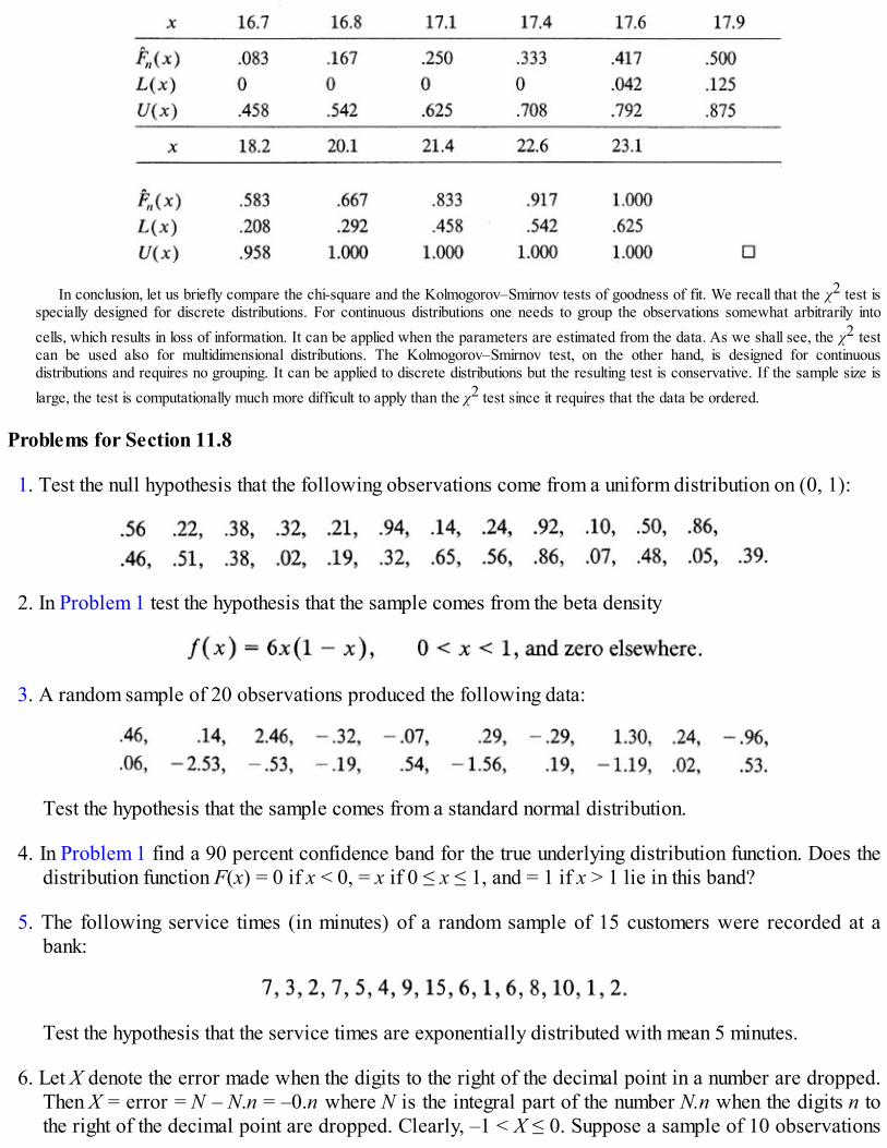
In conclusion, let us briefly compare the chi-square and the Kolmogorov–Smirnov tests of goodness of fit. We recall that the χ2 test isspecially designed for discrete distributions. For continuous distributions one needs to group the observations somewhat arbitrarily intocells, which results in loss of information. It can be applied when the parameters are estimated from the data. As we shall see, the χ2 testcan be used also for multidimensional distributions. The Kolmogorov–Smirnov test, on the other hand, is designed for continuousdistributions and requires no grouping. It can be applied to discrete distributions but the resulting test is conservative. If the sample size islarge, the test is computationally much more difficult to apply than the χ2 test since it requires that the data be ordered.

Problems for Section 11.8

1. Test the null hypothesis that the following observations come from a uniform distribution on (0, 1):

2. In Problem 1 test the hypothesis that the sample comes from the beta density

3. A random sample of 20 observations produced the following data:

Test the hypothesis that the sample comes from a standard normal distribution.

4. In Problem 1 find a 90 percent confidence band for the true underlying distribution function. Does thedistribution function F(x) = 0 if x < 0, = x if 0 ≤ x ≤ 1, and = 1 if x > 1 lie in this band?

5. The following service times (in minutes) of a random sample of 15 customers were recorded at abank:

Test the hypothesis that the service times are exponentially distributed with mean 5 minutes.

6. Let X denote the error made when the digits to the right of the decimal point in a number are dropped.Then X = error = N – N.n = –0.n where N is the integral part of the number N.n when the digits n tothe right of the decimal point are dropped. Clearly, –1 < X ≤ 0. Suppose a sample of 10 observations

on X showed the following results:

Test the hypothesis that the distribution function of X is uniform on ( – 1, 0].

7. In order to test the claim that the Scholastic Aptitude Test scores in mathematics for a certain group ofstudents have a normal distribution with mean 500 and standard deviation 70, a random sample of 12students from this group was taken and their SAT scores recorded as follows:

Is the claim justified?

8. Find a 95 percent confidence band for the distribution function of SAT mathematics scores in Problem7.

9. The times to failure (in hours) of 10 randomly selected 9-volt transistor batteries of a certain brandwere recorded as follows:

Test the hypothesis that the failure times are exponentially distributed with mean 45 minutes.

11.9 MEASURES OF ASSOCIATION FOR BIVARIATE DATA

In many practical problems involving pairs of measurements it is frequently of interest to study therelationship between the two sets of measurements. For example, are heights and weights of newbornsdependent? Is there any relationship between the college entrance test scores and freshman grade pointaverages? Are dose level of an antihypersensitive drug and blood pressure dependent?

Let X and Y be two jointly distributed random variables. We have seen in Section 5.2 that thecovariance between X and Y in a certain sense measures the interrelationship between X and Y. Forexample, the covariance is large and positive if large (small) values of X occur with large (small) valuesof Y with a high probability. We note that covariance is sensitive to the scales of measurement used. Forthis reason we defined the correlation coefficient between X and Y as

which is invariant under location and scale changes.If X and Y are independent ρ(X, Y) = 0, but the converse is not true. If X and Y are independent there is

no relationship or association between X and Y. On the other hand, if X and Y are associated in some wayor dependent, p may still be zero [except in the case when (X, Y) has a bivariate normal distribution].Thus, except in the bivariate normal case p may not be such a good measure of association between X andY.

Often the null hypothesis of interest is that X and Y are not associated, to be tested against thealternative hypothesis that they are associated. Under H0, X and Y are independent so ρ = 0 and it istempting to test instead. If then is accepted and we conclude that ρ = 0, it does notfollow that H0 is true. If, however, is accepted then it does follow that H1 is true, that is, that

X and Y are associated.In this section we consider two measures of association between X and Y which will also be used to

test the existence of an association between X and Y. In the special case when (X, Y) has a bivariatenormal distribution ρ does serve as a measure of association, and we have seen in Example 11.4.3 that thesample correlation coefficient given by

may be used to test H0 : ρ = 0 against one-sided or two-sided alternatives. We record the results belowfor completeness.

Likelihood Ratio Test of ρ = 0 when (X, Y)Has a Bivariate Normal Distribution

where r0 is the observed value of R given by (1) and P-value is computed by using the t-statistic with n – 2 d.f.

Example 1. Testing for Independence . A random sample of 12 observations from a bivariate normal distribution yielded a samplecorrelation coefficient of r0 = .68. Are X and Y independent? We wish to test H0 : ρ = 0 against H1 : ρ ≠ 0. We have

so that P-value = 2PH0(t(10) > 2.93), which is between .01 and .02. [Here t(10) has t-distribution with 10 d.f.] Thus H0 is rejected at

levels α ≥ .02 and we conclude that ρ is significantly different from zero. That is, X and Y are not independent.

11.9.1 The Spearman’s Rank Correlation Coefficient

The Spearman’s rank correlation coefficient is essentially the sample correlation coefficient R defined in(1) with X’s and Y’s replaced by their ranks. We assume that there are no ties among the X’s or among theY’s. Let R(Xi) be the rank of Xi among the X’s and R(Yi) be the rank of Yi among the Y’s, and let Di = R(Xi)– R(Yi). Then

and

Note, however, that

and

It follows from (2) that

Replacing Xi’s and Yi-’s by their ranks in (1) and writing RS for the resulting correlation coefficient, wehave

where we have used the fact that

Spearman’s Rank Correlation Coefficient

Let R(Xi) = Rank of Xi in the X’s and R(Yi) = Rank of Yi in the Y’s. Then

Note that the rankings of the X’s and Y’s are in complete agreement if and only if R(Xi) = R(Yi) foreach i, and in perfect disagreement if and only if R(Xi) = n + 1 – R(Yi) for each i. The difference Dibetween R(Xi) and R(Yi) measures the degree of disagreement between R(Xi) and R(Yi) in the sense that Di= 0 when R(Xi) = R(Yi), and the larger the |Di| (or ) the greater the disagreement. Thus is a measure of the disagreement between the two sets of ranks. Since large values of areassociated with small values of RS it follows that small values of RS tend to support the null hypothesis ofno association between X and Y. We note that |RS| = 1 indicates a perfect association and RS = 0 means noassociation. When RS = 1 there is a direct perfect agreement and when RS = – 1 there is an inverse perfectdisagreement. Hence large (positive) values of RS tend to support the alternative that there is a directassociation and large negative values of RS support the alternative that there is an indirect association. If|RS| is too large then the two-sided alternative that some association exists is supported.

Spearman’s Test for H0 : X and Y Are Not Associated

Here r0 is the observed value of RS.

In order to compute the P-value we note that RS has a symmetric distribution under H0. Table A13 inthe Appendix gives the right tail probabilities PH0

(RS ≥ r) for n ≤ 10 and all possible r values. The lefttail probabilities are obtained by symmetry. For values of n = 11, 12, …, 30, the table gives the smallestvalue of R (or the largest value of –R) for which the right tail (left tail) probability is at most .1, .05, .025,.01, .005.

For larger n (> 30) the statistic

has approximately a standard normal distribution. In case of a small number of ties one assigns theaverage rank to tied observations and uses the same null distribution to compute an approximate P-value.

Remark 1. The observations (Xi, Yi) need not be numerical as long as it is possible to rank the X’s andY’s. In many investigations two judges are asked to rank a group of subjects. In that case we can use RS toassess the degree of agreement between the two rankings.

Example 2. Dance Contest. Two judges rated the participants in a dance contest as follows.

A question of interest is, how closely do the two judges agree in their ratings? Computing the differences di between correspondingrankings we get

so that and

Since rS > 0 we note that the relationship is direct. Suppose we wish to test H0 : no association, against H1: direct association. Then theassociated P-value is given by

and we have to conclude that such a high value of RS could not have been obtained by chance under H0. That is, the data do support adirect association between the two rankings.

Example 3. Relationship Between Age and Weight of Premature Infants . Is there a direct relationship between the ages andweights of premature infants? In order to answer this question a random sample of 11 infants was taken and their ages and weights wererecorded as follows:

Since there are ties in ages as well as weights, we assign average ranks to tied observations.

We have and

which indicates a strong direct relationship between ages and weights of premature infants. Indeed,

It should be pointed out, however, that the number of ties in this example is not small. In general the value of RS is underestimated by

formula (4) in case of ties, and one needs to apply a correction for ties.† It is not necessary to do so in our example since it will onlyincrease the value of rS. We will not give a formula for this correction here.

11.9.2 Kendall’s Tau Statistic

Kendall’s tau statistic is also based on the ranks of X’s and Y’s. However, the test statistic is a function ofthe number of concordant and discordant pairs. We say that two pairs (xi, yi) and (xj, yj) (i ≠ j) areconcordant if both members of one pair are larger than their respective members of the other pair. Thatis, (xi, yi) and (xj, yj) are concordant if and only if

The pairs (xi, yi) and (xj, yj), i ≠ j, are said to be discordant if and only if

The pairs with ties between (one or both) respective members are neither concordant nor discordant.Thus the pairs (1.2, 1.9), (2.7, 2.0) and also the pairs (2.4, 1.3) (2.1, 1.1) are concordant, whereas thepairs (1.2, 1.9) and (2.7, 1.6) are discordant. The pairs (1.2, 1.8) and (1.3, 1.8) are neither concordantnor discordant. Let

and

Then

The measure of association proposed by Kendall is given by

If all pairs are concordant, then Nc = , Nd = 0 and τ = 1. If all pairs are discordant then Nd = and τ= – 1. If τ = 0, then there is no association since the number of pairs that are concordant is the same asthose that are discordant. Thus |τ| ≤ 1 and intermediate values of r reflect the degree of association. Thelarger the numerical value of τ the greater the degree of association.

Under the assumption that (X, Y) has a continuous distribution, ties occur with probability zero so thatP(N0 = 0) = 1 and

In that case

Whenever ties are present, we have to use (5) to compute τ. Otherwise one can use (6). The computationof τ in (6) is simplified by arranging (xi, yi) according to increasing values of x. Then each y is comparedwith those y’s that are below it to determine the number Nd. The number Nc is similarly computed.

Kendall’s Tau Statistic for Testing H0: NoAssociation Between X and Y

Compute where Nc is the number of concordant pairs and Nd is the numberof discordant pairs.

where τ0 is the observed value of τ.

In order to compute the P-value one needs the null distribution of τ. Table A14 in the Appendix givesthe right tail probabilities PH0

(τ ≥ τ0) for n = 3, 4, …, 20 computed under the assumption that there are noties. Since the distribution of τ is symmetric, the same table may be used for the left tail probabilities. Incase of ties the same table may be used but the resulting test is approximate and conservative. For n = 21,22, …, 40 exact tables are available but not given here. We give only the exact quantile values of the nulldistribution of τ for some selected tail probabilities. For n > 40, the statistic

has approximately a standard normal distribution so that approximate P-values may be computed from atable of normal distribution.

Example 4. Dance Contest (Example 2). In Example 2, two judges in a dance contest rated the participants as follows:

In order to compute Nc let us arrange the ranks for Judge 1 in their natural order as follows.

We now compare each rank for Judge 2 with those that are above it. Thus there are six ranks larger than 2, six ranks larger than 1, andso on. It follows that

In view of (6)

Similarly, Nd is the total number of ranks for Judge 2 that are smaller than and to the right of each successive rank. Thus, there is one

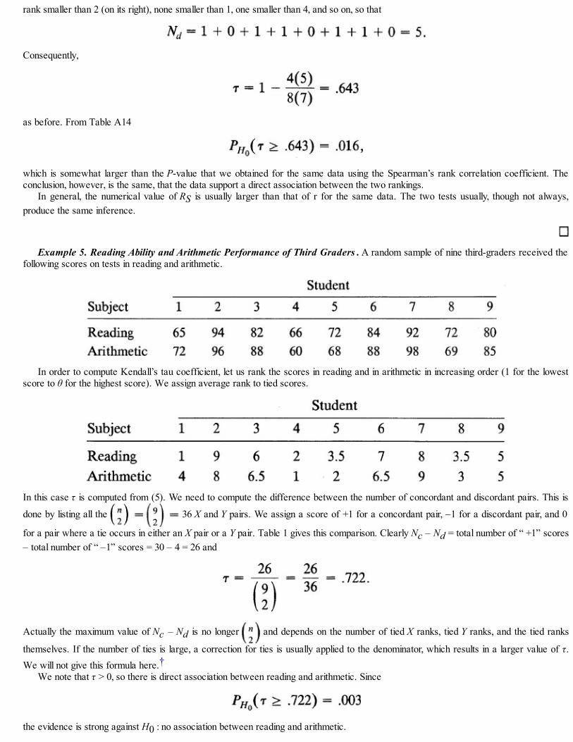
rank smaller than 2 (on its right), none smaller than 1, one smaller than 4, and so on, so that

Consequently,

as before. From Table A14

which is somewhat larger than the P-value that we obtained for the same data using the Spearman’s rank correlation coefficient. Theconclusion, however, is the same, that the data support a direct association between the two rankings.

In general, the numerical value of RS is usually larger than that of r for the same data. The two tests usually, though not always,produce the same inference.

Example 5. Reading Ability and Arithmetic Performance of Third Graders . A random sample of nine third-graders received thefollowing scores on tests in reading and arithmetic.

In order to compute Kendall’s tau coefficient, let us rank the scores in reading and in arithmetic in increasing order (1 for the lowestscore to θ for the highest score). We assign average rank to tied scores.

In this case τ is computed from (5). We need to compute the difference between the number of concordant and discordant pairs. This is

done by listing all the 36 X and Y pairs. We assign a score of +1 for a concordant pair, –1 for a discordant pair, and 0

for a pair where a tie occurs in either an X pair or a Y pair. Table 1 gives this comparison. Clearly Nc – Nd = total number of “ +1” scores– total number of “ –1” scores = 30 – 4 = 26 and

Actually the maximum value of Nc – Nd is no longer and depends on the number of tied X ranks, tied Y ranks, and the tied ranks

themselves. If the number of ties is large, a correction for ties is usually applied to the denominator, which results in a larger value of τ.We will not give this formula here.†

We note that τ > 0, so there is direct association between reading and arithmetic. Since

the evidence is strong against H0 : no association between reading and arithmetic.

TABLE 1. Computation of Scores

Problems for Section 11.9

1. At what levels are the following values of the sample correlation coefficient significant? (Assume thatthe sample comes from a bivariate normal distribution.)

(i) r = .35, n = 15, H0 : ρ = 0, H1: ρ > 0.(ii) r = .28, n = 17, H0 : ρ = 0, H1: ρ ≠ 0.(iii) r = –.64, n = 30, H0 : ρ = 0, H1 : ρ < 0.

2. A random sample of eight students was selected from the freshman class at a state university. For eachstudent the mathematics achievement test scores and the final score in the first calculus course wererecorded.

Assuming that the mathematics achievement scores and the calculus scores have a bivariate normaldistribution, is there evidence to conclude that the two scores are dependent?

3. Two judges ranked eight essays as follows:

Are the two rankings independent? Use both Kendall’s τ and Spearman’s rank correlation coefficient.

4. In order to test whether the heights of husband and wife are directly associated, a random sample ofeight couples was taken and their heights recorded.

(i) Compute the values of τ, RS and R.(ii) Test the claim that the heights are directly associated, using τ as well as RS.(iii) Assuming normality test H0 : ρ = 0 against H1 : ρ > 0.

5. Fifteen children were given two reading tests. Their relative rankings were as follows:

(i) Compute RS and τ. (ii) Is there evidence of a direct association?

6. The heights and weights of eight athletes are as follows:

(i) Compute R, RS, and τ.(ii) Assuming that height and weight have a joint normal distribution, test H0 : ρ = 0 against H1 : ρ >

0.(iii) Using RS and τ test to check whether there is evidence of a direct association between the

height and the weight of an athlete.

7. Seven applicants for the position of a probationary assistant professor were called in for interviews.Each applicant was assigned a rank by the chair in consultation with her advisory committee. Eachapplicant also saw the Dean, who also ranked the candidates. The following were the results of thesetwo rankings.

(Average rank was assigned by the Dean to applicants 1 and 5 since in his view they tied.) Test thehypothesis that there is no relationship between the two rankings.

8. Two preseason polls (of coaches and sportswriters) ranked the eight football teams in the Mid-American Conference as follows.

Test the hypothesis that there is a direct association between the two polls.

9. The following table gives the ages at inauguration and at death of the last 20 deceased Presidents ofthe United States of America.

President Age at Inauguration Age at DeathLincoln 52 56Johnson, A. 56 66Grant 46 63Hayes 54 70Garfield 49 49Arthur 50 56Clevelanda 47 71Harrison 55 67McKinley 54 58Roosevelt, T. 42 60Taft 51 72Wilson 56 67Harding 55 57

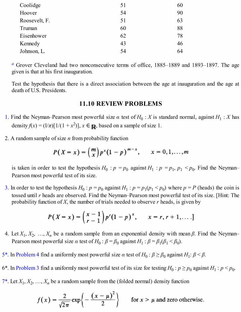
Coolidge 51 60Hoover 54 90Roosevelt, F. 51 63Truman 60 88Eisenhower 62 78Kennedy 43 46Johnson, L. 54 64

a Grover Cleveland had two nonconsecutive terms of office, 1885–1889 and 1893–1897. The agegiven is that at his first inauguration.

Test the hypothesis that there is a direct association between the age at inauguration and the age atdeath of U.S. Presidents.

11.10 REVIEW PROBLEMS

1. Find the Neyman–Pearson most powerful size α test of H0 : X is standard normal, against H1 : X hasdensity f(x) = (l/π)[1/(1 + x2)], x ∈ , based on a sample of size 1.

2. A random sample of size n from probability function

is taken in order to test the hypothesis H0 : p = p0 against H1 : p = p1, p1 < p0. Find the Neyman–Pearson most powerful test of its size.

3. In order to test the hypothesis H0 : p = p0 against H1 : p = p1(p1 < p0) where p = P (heads) the coin istossed until r heads are observed. Find the Neyman–Pearson most powerful test of its size. [Hint: Theprobability function of X, the number of trials needed to observe r heads, is given by

4. Let X1, X2, …, Xn be a random sample from an exponential density with mean β. Find the Neyman–Pearson most powerful size α test of H0 : β = β0 against H1 : β = β1(β1 < β0).

5*. In Problem 4 find a uniformly most powerful size α test of H0 : β ≥ β0 against H1: β < β.

6*. In Problem 3 find a uniformly most powerful test of its size for testing H0 : p ≥ p0 against H1 : p < p0.

7*. Let X1, X2, …, Xn be a random sample from the (folded normal) density function

Find a uniformly most powerful size α test of H0 : μ, ≤ μ0 against H1 : μ > μ0. Find the power functionof your test.

8*. An urn contains N balls of which D are colored white. A random sample of size n is taken. Let X bethe number of white balls in the sample. Find the form of the Neyman–Pearson most powerful test fortesting H0 : D = D0 against H1 : D = D1 (> D0). Find the form of the uniformly most powerful test of

against .

9*. Let X1, X2, … Xn be a random sample from probability function

Find the likelihood ratio test of H0 : p = p0 against H1 : p ≠ p0.

10*. Let X1, X2, …, Xn be a random sample from the density function

Find the likelihood ratio test of H0 : α = α0 against H1 : α < α0.

11*. Let where the Aj’s are disjoint and P(Aj) = pj > 0, j = 1, 2, …, k, .Suppose the experiment is repeated n times. Let Xj = number of times Aj happens, j = 1, 2, …, k. Then

. Find the likelihood ratio test of H0 : pi = , i = 1, 2, …, k against all alternatives.

12*. In Problem 11 suppose n is large so that –2ln λ(X1, ..., Xk) has approximately a χ2(k – 1) distribution.Show that the test based on –2ln λ is equivalent to the χ2 goodness of fit test based on the statistic

[Hint: Expand the logarithm and show that only the leading terms are important. That is, show that

where Rn → 0 (in probability) as n → ∞.]

13*. In the Hardy–Weinburg stability principle (see Problems 11.7.1 and 10.4.5), suppose a randomsample of n offspring shows that Xi offspring are of type i, i = 1, 2, 3, . [According to thestability principle, the offspring should be in proportions p1 = p2, p2 = 2p(1 – p), and p3 = (1 – p)2.]Show that the likelihood ratio test of H0 : p = p0 against H1 : p ≠ p0 is of the form: reject H0 if

where k1, k2 are constants.

14. The general manager of a discount department store chain of 12 stores is interested in finding outwhether shoelaces sell best when placed in the shoe department or when located at the checkoutcounter. Each store manager is asked to try a display of shoelace packages for four weeks in the shoedepartment and then switch it to the checkout counter for the next four weeks. The following resultswere obtained.

Is there evidence to conclude that the shoelaces sell better at the checkout counter? Use the sign testas well as the signed rank test to analyze the data.

15. Eighteen patients on a certain diet showed the following weight losses (in pounds):

Test the null hypothesis that the diet is ineffective (median weight loss is 0) against the alternativethat the diet is effective (median weight loss is positive). You may assume that the distribution ofweight loss is symmetric and continuous.

16. The median age of persons arrested for driving under the influence of alcohol (DUI) in a college townis believed to be 22 years. The sheriff believes that the median age of persons arrested for DUI islower. She takes a random sample of 10 such arrest records and finds the following ages:

Use the Wilcoxon signed rank test to test the claim that the median age of a DUI arrest is 22 yearsagainst the alternative hypothesis that the median age is lower. Also apply the sign test and compareyour results.

17. A teacher is concerned about the poor performance of students in her introductory statistics course.She believes that this is due to the poor mathematics background of her students. She selects a randomsample of 15 students in her class and divides them into two groups according to their mathematicsbackground. The final scores of these 15 students are as follows:

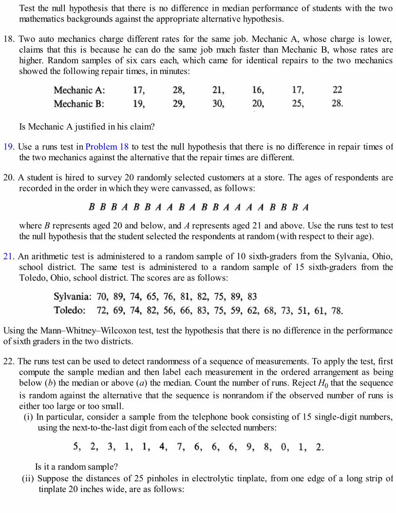
Test the null hypothesis that there is no difference in median performance of students with the twomathematics backgrounds against the appropriate alternative hypothesis.

18. Two auto mechanics charge different rates for the same job. Mechanic A, whose charge is lower,claims that this is because he can do the same job much faster than Mechanic B, whose rates arehigher. Random samples of six cars each, which came for identical repairs to the two mechanicsshowed the following repair times, in minutes:

Is Mechanic A justified in his claim?

19. Use a runs test in Problem 18 to test the null hypothesis that there is no difference in repair times ofthe two mechanics against the alternative that the repair times are different.

20. A student is hired to survey 20 randomly selected customers at a store. The ages of respondents arerecorded in the order in which they were canvassed, as follows:

where B represents aged 20 and below, and A represents aged 21 and above. Use the runs test to testthe null hypothesis that the student selected the respondents at random (with respect to their age).

21. An arithmetic test is administered to a random sample of 10 sixth-graders from the Sylvania, Ohio,school district. The same test is administered to a random sample of 15 sixth-graders from theToledo, Ohio, school district. The scores are as follows:

Using the Mann–Whitney–Wilcoxon test, test the hypothesis that there is no difference in the performanceof sixth graders in the two districts.

22. The runs test can be used to detect randomness of a sequence of measurements. To apply the test, firstcompute the sample median and then label each measurement in the ordered arrangement as beingbelow (b) the median or above (a) the median. Count the number of runs. Reject H0 that the sequenceis random against the alternative that the sequence is nonrandom if the observed number of runs iseither too large or too small.(i) In particular, consider a sample from the telephone book consisting of 15 single-digit numbers,

using the next-to-the-last digit from each of the selected numbers:

Is it a random sample?(ii) Suppose the distances of 25 pinholes in electrolytic tinplate, from one edge of a long strip of

tinplate 20 inches wide, are as follows:

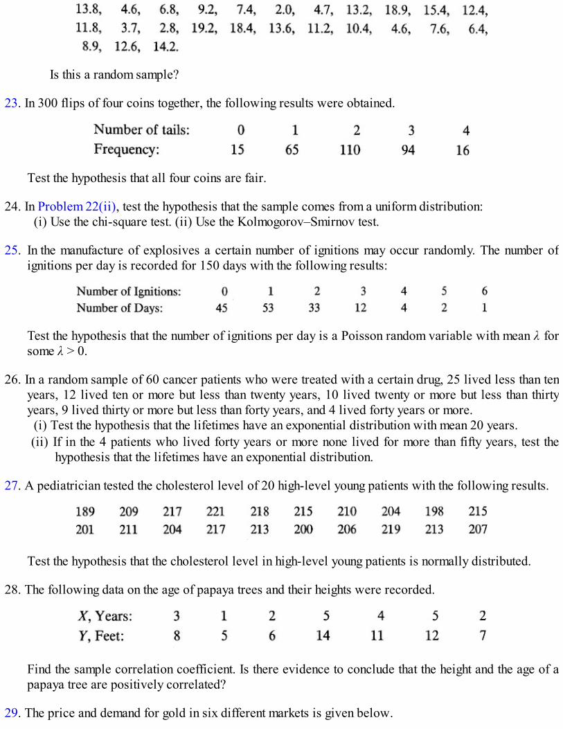
Is this a random sample?

23. In 300 flips of four coins together, the following results were obtained.

Test the hypothesis that all four coins are fair.

24. In Problem 22(ii), test the hypothesis that the sample comes from a uniform distribution:(i) Use the chi-square test. (ii) Use the Kolmogorov–Smirnov test.

25. In the manufacture of explosives a certain number of ignitions may occur randomly. The number ofignitions per day is recorded for 150 days with the following results:

Test the hypothesis that the number of ignitions per day is a Poisson random variable with mean λ forsome λ > 0.

26. In a random sample of 60 cancer patients who were treated with a certain drug, 25 lived less than tenyears, 12 lived ten or more but less than twenty years, 10 lived twenty or more but less than thirtyyears, 9 lived thirty or more but less than forty years, and 4 lived forty years or more.(i) Test the hypothesis that the lifetimes have an exponential distribution with mean 20 years.(ii) If in the 4 patients who lived forty years or more none lived for more than fifty years, test the

hypothesis that the lifetimes have an exponential distribution.

27. A pediatrician tested the cholesterol level of 20 high-level young patients with the following results.

Test the hypothesis that the cholesterol level in high-level young patients is normally distributed.

28. The following data on the age of papaya trees and their heights were recorded.

Find the sample correlation coefficient. Is there evidence to conclude that the height and the age of apapaya tree are positively correlated?

29. The price and demand for gold in six different markets is given below.

Find the sample correlation coefficient between the price of gold and the demand for gold.

30. A customer who regularly visits a particular restaurant for lunch rates the quality of food and serviceover a period of 25 consecutive days as good (g) or bad (b) as follows:

Test the null hypothesis that the quality of food and service at this restaurant is random.

31. Fifty successive light bulbs produced by a certain machine are examined to see if they are defective(D) or nondefective (N) with the following results:

Do the data indicate that the defective light bulbs occur randomly?

32. An educational scientist took a random sample of 15 fathers and sons and obtained the following datafor their intelligence quotients.

Is there evidence of a direct association between a father’s and son’s I.Q.? Apply both Spearman’sand Kendall’s tests.

33. A random sample of nine middle-income families of four showed the following data on the monthlyfood cost and disposable income (in dollars).

Is there evidence of a direct relationship between the monthly disposable income and food costs?

† For details, see J. D. Gibbons, Nonparametric Methods for Quantitative Analysis, Holt, Rinehart and Winston, New York, 1976, p. 279.† For details, see J. D. Gibbons, Nonparametric Methods for Quantitative Analysis, Holt, Rinehart and Winston, New York, 1976, p. 289.

CHAPTER 12

Analysis of Categorical Data

12.1 INTRODUCTION

Suppose each observation in a random sample is classified as belonging to one of a finite number ofmutually exclusive classes or categories. For example, the family income may be classified as belongingto one of the five classes: poor ($10,000 or less), lower middle class (between 10 and 20 thousanddollars), middle class (20–30 thousand dollars), upper middle class (30–40 thousand dollars), andaffluent (more than $40,000). Let pi = P(an observation is in category i). The object may be to test the nullhypothesis H0: pi = p0

i, i = 1, 2, …, k when p0i are completely specified. The reader will recognize that

H0 can be tested by using the X2 test of goodness of fit studied in Section 9.9 (when p0i’s are prespecified)

and Section 11.7 (when p0i’s are specified except for some unknown parameter which has to be estimated

from the data).The chi-square test applies also to the case when we wish to test that

(i) the pi’/s are the same for several different populations, or(ii) family income is independent, say, of the geographical region in which a family resides.

In the former case we take independent random samples from the J-populations being compared, and theobject is to test H0: pi1 = pi2 = ⋯ = pi, J, i = 1, 2, …, k, against all possible alternatives. The X2 test isspecially designed for discrete data and it tests homogeneity of the J populations against generalalternatives. This test is studied in Section 12.2. In the latter case we have one sample from a populationcategorized in two ways (for example, according to family incomes and according to geographic region).The resulting cross-categorized data can be put in a so-called contingency table with the object of testingH0: The two categorical variables are independent. This test is studied in Section 12.3.

12.2 CHI-SQUARE TEST FOR HOMOGENEITY

Suppose we have two or more populations and we wish to test the null hypothesis that they all have thesame distribution. In Section 11.6 we considered two well known tests for testing the equality of twodistribution functions. These tests assume that the underlying distributions are continuous and do noteasily extend to the case of more than two populations. The test that we consider here is speciallydesigned for discrete populations although it applies also to continuous populations.

Let us begin with a simple case. Suppose we have two coins and we wish to test H0: p1 = p2 = p(known) against all possible alternatives where p1, p2 are the respective success probabilities. Supposewe toss the first coin n1 times and observe X successes and the second coin n2 times and observe Ysuccesses. These results can now be put in a 2 × 2 contingency table as follows:

TABLE 1

We assume that the n1 + n2 trials are independent. According to Section 9.9, under H0, the statistics

and

are independent random variables each of which, for large n1 and n2, has approximately a chi-squaredistribution with 2 – 1 = 1 d.f. Hence their sum is itself a Χ2 random variable with 2 d.f. Note, however,that

so that

has approximately a Χ2 distribution with 2 d.f. In complete analogy to the development in Section 9.9,therefore, we reject H0: p1 = p2 = p at level α if

The case of most interest is when the common value of p1 and p2, under H0, is unknown. In that case themaximum likelihood estimate of p is given by

According to Theorem 11.7.1 (and the discussion following it) if we substitute for p in the expression

for Q in (1), then the resulting test statistic Q( ) has an approximate Χ2 distribution with 2 – 1 = 1 d.f.since we estimated one parameter from the sample. We have

We therefore reject H0: p1 = p2 at level α if Q( ) > Χ21, α.

When n1, n2 are large, we saw in Section 9.7 that the statistic

has, under H0, approximately a standard normal distribution. Are the tests based on Z given in (4) and Qgiven in (3) equivalent? The answer is yes. Indeed, Z2 has approximately a Χ2(1) distribution. Moreover,

We can rewrite Q in a more recognizable form:

In terms of Table 1, it means that to compute Q we cross-multiply the table entries, take the difference andsquare it, multiply it by the total number of observations, and then divide by the product of row andcolumn totals.

Example 1. Faculty Attitudes Toward Teaching Loads . Independent random samples of 50 faculty members from the Colleges ofArts and Sciences and Business at a State University were asked whether they felt that the teaching loads were reasonable orunreasonable. The following results were obtained.

Let us test the hypothesis that the faculty in the two colleges have the same attitude toward teaching loads. We have

Under H0, we note that

and there is sufficient evidence in support of H0.Let us also apply the normal theory test of Section 8.7. We have

so that

and the P-value is .2202. This result is consistent with the result based on the Χ2 test. Indeed, q0 = 1.45 z2, as it must.

The outline for the general case should now be evident. Let us suppose that we have J independentmultinomial distributions. That is, suppose we have k categories A1, A2, …, Ak and J independent samplesof sizes n1, n2, …, nJ respectively. Let Xij be the number of times Ai happens in the jth sample, i = 1, 2,…, k, j = 1, 2, …, J. The data can be put in a k × J contingency table as follows:

TABLE 2

Let pij = Pj(Ai) , i = 1, 2, …, k, j = 1, 2, …, J where Pj refers to the probability under the jthpopulation. The hypothesis of homogeneity of the J populations that we wish to test is H0: pi1 = pi2 = … =PiJ, i = 1, 2, …, k, against all possible alternatives. We consider the case of most interest where, underH0, the common value pi of the pij’s is unknown. The maximum likelihood estimates of the pis are easilyshown to be

and , where and . We note that we haveestimated k – 1 parameters. In view of Theorem 11.7.1 we note that the statistic

has, for large n, an approximate chi-square distribution with d.f. given by

The argument used here is simple. If the pi’s are known, then

is the sum of J independent (approximate) Χ2(k – 1) random variables so that it has an approximate Χ2(J(k– 1)) distribution. Since we estimated k – 1 parameters, we lose k – 1 d.f.

Although the above procedure has been specially designed to test the equality of two or moremultinomial distributions, it can be adapted to test the equality of two or more continuous distributionfunctions. Let us take J = 2 for convenience. We wish to test H0: F(x) = G(x) for all x against H1: F(x) ≠G(x) for some x. We have already considered (Section 11.6) some special tests designed to test thishypothesis. Let X1, X2, …, Xn1

and Y1, Y2, …, Xn2 be independent random samples from F and G

respectively. Partition the real line into k disjoint intervals A1, A2, …, Ak and let

Under H0 we note that pi1 = pi2 for i = 1, 2, …, k. We test the less restrictive hypothesis against all possible alternatives. Then the appropriate test statistic is

where Xi1 = number of Xj’s that fall into Ai, and Xi2 = number of Yj’s that fall into Ai, i = 1, 2, …, k and .

In applications, the question arises how the intervals Ai’s are selected. This question has already beenanswered in Section 9.9.

Example 2. Sex Differences in Incidence and Amount of Aggression . In Problem 11.6.4 the reader was asked to test if there isevidence to suggest that there are sex differences in the incidence and amount of aggression in three-year-olds. The following scoreswere recorded:

Boys: 96, 65, 74, 78, 82, 121, 68, 79, 111, 48, 53, 92, 81, 31, 48Girls: 12, 47, 32, 59, 83, 14, 32, 15, 17, 82, 21, 34, 9, 15, 50

Let us divide the scores in three classes of equal length, namely A1 = [8, 42], A2 = [43, 77], A3 = [78,112]. We have the following result:

Then the estimates of p1, p2, p3 are given by

and

For (3 – 1)(2 – 1) = 2 d.f. we note that

and the two distributions are significantly different at 1 percent level. This result is consistent with theresult of Problem 11.6.4.

Example 3. Television Viewing Preference . A market analyst believes that there is no difference in preferences of televisionviewers among the four Ohio cities of Toledo, Columbus, Cleveland, and Cincinnati. In order to test this belief, independent randomsamples of 150, 200, 250, and 200 persons were selected from the four cities and asked, “What type of program do you prefer most:Mystery, Soap, Comedy, or News Documentary?” The following responses were recorded.

Under the null hypothesis that the proportions of viewers who prefer the four types of programs are the same in each city, themaximum likelihood estimates of pi, i = 1, 2, 3, 4 are given by

Here p1 = proportion of people who prefer mystery, and so on. The following table gives the expected frequencies under H0.

It follows that

Since J = 4 and k = 4, the number of degrees of freedom is (4 – 1)(4 – 1) = 9 and we note that under H0

With such a large P-value we can hardly reject H0. The data do not offer any evidence to conclude that the proportions in the four citiesare different.

In conclusion, we emphasize that the Χ2 test studied in this section is a test designed for categoricaldata, and it tests the equality of J proportions against general alternatives. In a specific problem we maybe more interested in testing the null hypothesis against restricted alternatives such as pi1 > pi2 > ⋯ > piJ

for i = 1, 2, …, &, k … 1. Any test specifically designed for this purpose will usually perform better thanthe Χ2 test of homogeneity. Similarly, tests designed for testing equality of several continuous distributionfunctions should perform better than the Χ2 test. (Such tests are studied in Chapter 13.)

Problems for Section 12.2

1. Three dice are rolled independently 360 times each with the following results.

Are all the dice equally loaded? That is, test the hypothesis H0: pi1 = pi2 = pi3, i = 1, 2, …, 6, wherepi1 is the probability of getting an i with die 1, and so on.

2. Three different methods of instruction were used to teach a calculus course. In order to compare theeffectiveness of the three methods, 45 comparable students were divided into three groups of 15 each.Each group was taught using one of these three methods. After the semester a standardized test wasgiven and the following scores were recorded.

Test the equality of the distributions of test scores. (Partition the combined sample of 45 scores intothree equal parts, each part containing 15 scores by taking the intervals [37, 62.5), (62.5, 76.5),(76.5, 92].)

3. Three independent random samples are taken with the following results:

(i) Test the hypothesis that the samples come from a standard normal distribution. You may useintervals A1 = (–∞, –.75], A2 = (–.75, 0), A3 = [0, .75), A4 = [.75, ∞).

(ii) Using the same intervals as in part (i), test the hypothesis that the three samples come from thesame population.

4. Independent random samples of 250 Democrats, 150 Republicans, and 100 Independent voters wereselected one week before a nonpartisan election for mayor of a large city. Their preference forcandidates Albert, Basu, and Chatfield were recorded as follows.

Are the proportions of voters in favor of Albert, Basu, and Chatfield the same within each politicalaffiliation?

5. An outpatient clinic at the County Health Center conducted an experiment to determine the degree ofrelief provided by three pain relievers. Each pain reliever was given to 75 patients with the followingresults:

Is there evidence to conclude that the three pain relievers are equally effective?

6. Independent random samples of 50 students each were selected from the colleges of Arts and Sciences,Music, Business, Engineering, and Law at a large state university in order to determine whether thereis a difference in proportions of students in the colleges who favor a proposal to have a studentrepresentative on the Board of Trustees. The following responses were recorded.

Is there evidence to conclude that the proportions of students in favor of representation is the samefor these five colleges?

7. It is believed that the level of education that an 18-year-old man has received strongly influences hisattitude toward the draft. Independent random samples were drawn of 100 men with only elementaryschool education, 100 with a high school diploma, and 75 with at least a year of college. Thefollowing data were collected.

Is there sufficient evidence to conclude that the distribution of the attitudes toward the draft differsamong the three populations?

8. Independent random samples of 280 divorced males and 350 divorced females resulted in thefollowing age distribution.

Is there sufficient evidence to conclude that the age distributions of divorced males and females arethe same?

9. Independent random samples of 100 immigrants from Europe, 150 immigrants from the Far East, and200 immigrants from Southeast Asia were taken after one year of their arrival into the United States.Their annual incomes were recorded as follows.

Is there sufficient evidence to conclude that the distribution of annual income is the same for eachgroup of immigrants?

10. Let (X11, X12, …, Xk1), …, (X1J, X2J, …, XkJ) be independent multinomial random variables withparameters (n1, p11, p12, …, pk1), … ,(nJ, p1J, p2J, …, pkJ) respectively. Let

and n. Show that thelikelihood ratio statistic for testing H0: pij = pi, j = 1, 2, …, J, i = 1, 2, …, k where pi are unknownagainst all alternatives is given by

12.3 TESTING INDEPENDENCE IN CONTINGENCY TABLES

In Section 11.9 we defined some measures of association between two sets of measurements and usedthese to test the null hypothesis that the two sets of measurements are not associated and (henceindependent). The Χ2 statistic can also be used to yield a test for independence. The test is speciallydesigned for categorical data, although it can be adapted for use in the case of continuous data. The datafor analysis therefore are frequency counts in each cross-category as against the rank data used in Section11.9. The test answers questions of statistical interest such as: Is the color of a person’s eyes independentof his or her hair color? Are the opinions of voters on a particular issue independent of their politicalviews?

Consider a random experiment where each outcome can be categorized by two different attributes(such as height and weight, or level of education and annual income). Let A1, A2, …, Ar be the r mutuallyexclusive and exhaustive categories of the first attribute and let B1, B2, …, BC be the c mutually exclusiveand exhaustive categories of the second attribute. Write

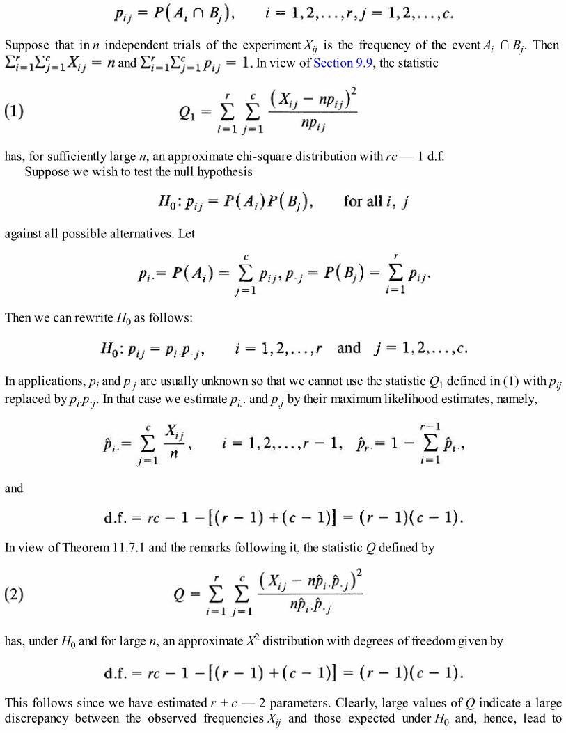
Suppose that in n independent trials of the experiment Xij is the frequency of the event Ai ∩ Bj. Then and In view of Section 9.9, the statistic

has, for sufficiently large n, an approximate chi-square distribution with rc — 1 d.f.Suppose we wish to test the null hypothesis

against all possible alternatives. Let

Then we can rewrite H0 as follows:

In applications, pi and p.j are usually unknown so that we cannot use the statistic Q1 defined in (1) with pijreplaced by pi.p.j. In that case we estimate pi.. and p.j by their maximum likelihood estimates, namely,

and

In view of Theorem 11.7.1 and the remarks following it, the statistic Q defined by

has, under H0 and for large n, an approximate Χ2 distribution with degrees of freedom given by

This follows since we have estimated r + c — 2 parameters. Clearly, large values of Q indicate a largediscrepancy between the observed frequencies Xij and those expected under H0 and, hence, lead to

rejection of H0. The approximate P-value corresponding to the computed value q0 of Q is given byP(Χ2((r – 1)(c – 1)) ≥ q0). Bounds for this probability may be obtained from Table A7.

Let us examine the expression for Q in (2) a little more carefully. For convenience we write for the ith row total and for the jth column total. The r × c contingency

table now looks as follows.

TABLE 1. r × c Contingency Table

We note that Table 1 looks much like Table 2 in Section 12.2. An important difference, however, isthat in Table 2 of Section 12.2 the row totals are random variables while the column totals are fixed,whereas in Table 1 both the row and the column totals are random variables. Nevertheless, thecomputation of Q defined in (2) is exactly the same as that of Q defined in (12.2.7). Indeed,

so that Q defined in (2) can we rewritten as

This is precisely the expression for Q in (12.2.7) if we take r = k, c = J and X.j = nj. From acomputational point of view, therefore, the two expressions are the same. In fact, according to the law oflarge numbers for large n, the random column totals X.j in Table 1 will be approximately equal to np.j =nj, so that under the assumption of independence the cell frequencies in the jth column will have(approximately) a multinomial distribution with parameters nj and p1. , p2., … pr. for each j. This isprecisely the assumption of homogeneity of the c populations.

The test can be easily adapted to test the independence of random variables X and Y when (X, Y) has acontinuous bivariate distribution. We partition the ranges of X and Y into mutually disjoint intervals A1,A2, …, Ar and B1, B2, …, BC. Given the sample (x1, y1), (x2, y2), ∆, (xn, yn) it is then an easy matter to put

the sample in the form of an r ∆ c contingency table such as Table 1. The cell count xij represents thenumber of pairs (xl, yt) for which xl ∈ Ai and yl ∈ Bj.

If, on the other hand, (X, Y) has a discrete distribution taking only a finite set of pairs of values, thenthe categories Ai and Bj are automatically determined respectively by the range of values of X and therange of values of Y.

Example 1. Smoking and Cause of Death. A random sample of 2100 death certificates of adults were examined in a largemetropolitan area and showed the following results.

Death by Causes and Smoking Habits

Is the cause of death independent of a person’s smoking habit?We will use expression (3) to compute Q. Under H0 that the cause of death is independent of a person’s smoking habit, we expect

Xi.X.j/n observations in cell (i, j). The following table shows the expected frequencies.

Expected Frequencies

Thus

For (3 – 1)(2 – 1) = 4 d.f. we see that

so that we have to reject H0 and conclude that the cause of death of a person depends on his or her smoking habit.

Example 2. Ages at Inauguration and at Death of U.S. Presidents . The following pairs of observations represent the ages atinauguration and at death of the 35 U.S. Presidents.

In Problem 11.9.9 we asked the reader to test the hypothesis that there is a direct association between the age at inauguration and the ageat death (using a subset of 20 observations). The Χ2 test that we apply here will only test whether the two random variables areindependent. We note that the ages at inauguration range from 42 to 68 and the ages at death range from 46 to 90. Let us choose theintervals

and

We get the following 3 × 3 contingency table where the numbers in parentheses give the expected cell counts under the hypothesis ofindependence.

Using the formula (3) we compute q0 = 10.99, and for (3 – 1)(3 – 1) = 4 d.f. we see that

Thus we reject H0 at level .05 (but not at level .025) and conclude that the age at inauguration and age at death of U.S. Presidents aredependent. It should be noted that the number of observations is quite small and, moreover, that several cells have relatively smallexpected cell frequencies.

Problems for Section 12.3

1. A random sample of 1000 employed individuals was taken and the distribution of their salary by sexwas found to be as follows:

Is the annual income of an employee independent of his or her sex?

2. The following data represent the blood types and ethnic groups of a random sample of 550 minoritycitizens of the United States.

Test the hypothesis that the blood type of a minority citizen is independent of his or her ethnic group.

3. A random sample of 500 individuals was taken to investigate whether smoking and alcohol drinkingare related. The following results were obtained.

Test the hypothesis that alcohol drinking and smoking are independent.

4. The score on the mathematics portion of the ACT (American College Test) examination and on the finalexamination in first semester Statistics course for a random sample of 150 students were classified asfollows:

Is there sufficient evidence to conclude that the ACT mathematics score X of a student is independentof the statistics score Y?

5. In a study, a random sample of 15 racing days were selected at a race track and the results of all theraces were classified according to the post position of the horse and the order in which it finished inthe race.

Is the order in which a horse finishes independent of its post position? (Note that marginal totals inthis case are predetermined and not random variables.)

6. The final grades that students thought they would receive in five Elementary Statistics courses taughtover five semesters were cross tabulated with the rating that the students gave the course. Thefollowing results were obtained.

Is the students’ rating of the course independent of the predicted grade?

7. In a survey of 350 employees, conducted to determine whether the annual salary of an employee isdependent on the length of his or her service, the following results were tabulated.

What is your conclusion?

8*. Consider an r × c contingency table with cell frequencies xij, i = 1, 2, …, r and j = 1, 2, …, c. Let pijbe the probability that a randomly selected observation falls in cell (i, j) and let

. The hypothesis of independence then can be written as:

Show that the likelihood ratio test statistic for testing H0 is given by

where and For large n, the statistic – 2ln λ(X)has, under H0, an approximate Χ2 distribution with (r – 1)(s – 1) d.f.

12.4 REVIEW PROBLEMS

1. A small college is discussing the possibility of dropping its athletics program. A random sample ofstudents, faculty, and administrative staff is taken in order to determine their reaction to the proposal.The results of the survey are as follows:

Test the hypothesis that the attitude toward the proposal is independent of the status of the individual.

2. In Problem 1, suppose independent random samples of 50 faculty, 200 students, and 25 administrativestaff members are taken in order to ascertain their opinion on whether or not the athletic programshould be dropped. Test the hypothesis that the proportions of individuals who are in favor, opposed,or have no opinion among the three groups are the same. The results of the survey are as follows.

3. A market opinion survey is conducted to determine if the weekly magazine that an individual trustsmost is related to his or her annual income. The following table gives the results of a sample of 500readers.

Test the hypothesis that the annual income of a reader is independent of the weekly magazine that heor she trusts most.

4. A statistical society sends a questionnaire to its members with the following results:

Is the rate of response independent of the type of employment of the member?

5. Independent random samples of 500 freshmen in the state university system and 500 freshmen in thetwo-year colleges in the state are taken with the following distribution.

Test the null hypothesis that the age distribution of freshmen is the same in the two-year colleges andthe state university system.

6. A survey is conducted to determine whether the incidence of certain types of crime in a largemetropolitan area depends on the location where the crime is committed. The following tablesummarizes the 1205 crimes committed during a three-month period by their location.

Does the type of crime depend on the location where it is committed?

CHAPTER 13

Analysis of Variance: k-Sample Problems

13.1 INTRODUCTION

In the previous chapters, we have devoted several sections to the problem of testing the equality of twodistribution functions. For example, the problem of testing the equality of two normal distributionfunctions was considered in Section 8.7. When the underlying populations are not normal, the sameproblem was considered in Section 11.6 and again in Section 12.2. The χ2 test of homogeneity is the onlytest considered so far which can be used to test the equality of several distributions. This test, however, isdesigned specially for testing the equality of several proportions and is an approximate test. One needs alarge sample size for the approximation to be good. Moreover, the test depends on how the observationsare grouped.

In practical applications one often needs to compare more than two populations (for example, morethan two brands of gasoline additives, or several methods of instruction, or several fertilizers, and so on).It is usual to call the different methods (or additives or fertilizers) treatments. The method of analysisdepends very much on the design of the experiment and the type of assumption one is willing to make. Letus consider the following example.

Suppose we wish to compare the average number of units produced per day by four differentmachines (treatments). First suppose that the same worker is asked to operate the four machines so thatthere is no variation due to the manner in which the machines are operated (that is, due to the worker).Suppose we wish to have a total of n experimental units (that is, a total of n observations). If n1 units arerandomly assigned to treatment 1 (that is, n1 observations are taken on machine 1), n2 to treatment 2, n3 totreatment 3, and n4 to treatment 4, then we have what is known as a completely randomized design. Theanalysis of such a design depends on the type of assumptions we are willing to make about theobservations. If we assume that each of the four samples comes from a normal population with the same(unknown) variance, then the data is analyzed by one-way analysis of variance, which is an extension ofthe two-sample t-test. One-way analysis of variance is considered in Section 13.2. In Section 13.3 weconsider a procedure for constructing simultaneous confidence intervals for the difference μi – μj in meansμi and μj of the ith and the jth treatments for all i ≠ j. This allows us to identify the means that aresignificantly different.

If, on the other hand, we assume only that the samples come from continuous distribution functions,then we can use either an extension of the two-sample median test or an extension of the Mann–Whitney–Wilcoxon test. Both these methods are considered in Section 13.5. We also consider a multiplecomparison procedure, analogous to the one introduced in Section 13.3, that allows us to identifysignificantly different treatments.

Next suppose that different workers are asked to operate each of the four machines. In this case thereis a variation due to the workers as well as one due to the machines. Indeed, there may also be variationdue to interaction between the machines and the workers. A special case is when we have a total of nexperimental units subdivided into b homogeneous groups called blocks (in our case each worker

represents a block so that b = number of workers). Each block has four different units corresponding tofour different treatments, so that n = 4b. This is the so-called randomized complete block design. Theanalysis of such a design in the special case when we assume normality (and also in the case when wehave several observations in each block) is carried out by a two-way analysis of variance. Section 13.4deals with this topic. If we drop the assumption of normality, then we need an extension of the pairedcomparison techniques of Section 11.9. This so-called Friedman test is studied in Section 13.6.

13.2 ONE-WAY ANALYSIS OF VARIANCE

Suppose three sections of the same Elementary Statistics course are taught by three instructors. The finalgrades of students in the three sections are recorded as follows:

Is the distribution of grades the same in the three sections? Suppose we are willing to assume that thegrades in each section are normally distributed and, moreover, the variances of the distributions of gradesin the three sections are the same. Since a normal distribution is completely determined by its mean andthe variance, the problem of testing the equality of the three distributions reduces to the problem of testingthe equality of the three means. In mathematical language, therefore, the problem may be posedequivalently as follows:

Let X11, X12, …, X1n1, X21, X22, …, X2n2

, and X31, X32, …, X3n3 be independent random samples from

three normal populations with respective parameters μ1 and σ12, μ2 and σ2

2, and μ3 and σ32. Suppose σ1 =

σ2 = σ3. How do we test the null hypothesis

against the alternatives that either μ1 and μ2, or μ1 and μ3, or μ2 and μ3, or μ1 and μ2 and μ3 are unequal?Let us first explain why the methods of Section 8.7 cannot be used here. According to Section 8.7 we

can test the equality of μ1 and μ2 by using the t-statistic

where

and

In order to apply this procedure we would have to run a sequence of t-tests on each of the null hypothesesμ1 = μ2, μ2 = μ3, and μ3 = μ1. If any of these hypotheses were rejected then we would conclude that themeans are not all the same. This, however, is a very inefficient way to proceed. Suppose we ran the threet-tests at sizes α1, α2, and α3 respectively. Let A1, A2, and A3 respectively be the acceptance regions ofthese tests. Then

The probability of accepting H0: μ1 = μ2 = μ3 is given by pH0(A1 ∩ A2 ∩ A3), so that the probability of

rejecting H0 when true is given by 1 – PH0(A1 ∩ A2 ∩ A3). If A1, A2, and A3 were independent events

(which would be the case if the three test statistics were independent), then

If, for example, αi = .05, i = 1, 2, 3, then

so that the size of the combined test is considerably larger than the size of each of the three tests. In ourcase the Ai’s are not independent, and we do not know what the overall α is. We do know from Boole’sinequality (2.4.13) that

Moreover,

Note also that in comparisons of k samples taken two at a time, some will be significant by

chance. For example, in 100 such comparisons by t-test we expect about five to be significant at level .05even if there were no real differences among the means.

Thus the temptation to apply a sequence of t-tests to the data should be avoided. See also Remark8.7.1.

The two-sample case, however, does provide a clue to how we should proceed in the (general) caseunder consideration. Let us therefore analyze the two-sample case a little more carefully.

Recall (Problem 8.8.27 or the definition of an F-statistic given in Example 8.4.6) that T2 has an Fdistribution with (1, n1 + n2 – 2) d.f. Hence the t-test is equivalent to the test based on the statistic

Let us write

for the sample mean of the n1 + n2 observations in the combined sample. Then

Also,

so that the quantity [n1n2/(n1 + n2)](X1 – X2)2 in the numerator of the expression for F in (2) is simply , the weighted sum of squares of deviations of sample means from the grand mean X.

Also, the quantity in the denominator of F can be written in the form

Under H0, μ1 = μ2, so that the two samples come from the same population and X is the best estimateof the common unknown mean. The total variation in the combined sample is therefore measured by thetotal sum of squares (TSS) given by

Let us now split up TSS as follows:

since . In view of (4), (5), and (7) we have

Figure 1. Partitioning the total variation. Dots represent individual observations.

In expression (8) we have partitioned the total variation in the combined sample into two parts (seeFigure 1). The first part on the right side of (8) or of (7) is the so-called error sum of squares (SSE)which is used to give a pooled estimate of the common unknown variance. It measures the variationwithin samples. The second part,

is the so-called treatment sum of squares (SST) which measures the variation among the samples. Thelarger the treatment sum of squares the greater the evidence against H0. It follows that large values of theratio

lead to the rejection of H0. This is essentially the test based on T2. The reason we have S2 in thedenominator of T2 is to give an F distribution for the ratio that allows us to determine what values of theratio will be significant at level α.

Yet another way to look at the same problem is to compare the two estimates of α2 (the commonunknown variance). Under H0: α1 = α2 we have

so that SST provides an unbiased estimate of α2. Also [see (8.7.7) and the computation following it],

whether H0 is true or not so that SSE/(n1 + n2 – 2) is also an unbiased estimate of α2. When the nullhypothesis is false we expect the estimate SST of α2 to exceed (Problem 9) the estimate S2 = SSE/(n1 + n2

– 2), and hence the null hypothesis will be rejected at level α if the ratio F = T2 exceeds the (1 – α)thquantile of the F distribution for (1, n1 + n2 – 2) d.f.

This analysis of the two-sample case suggests how we should proceed in the general case: partitionthe total variation in the combined sample into two parts. One part explains the variation between thesamples while the second part explains the variation within each sample. Compare the two. Equivalently,find two estimates of the common variance, one based on the deviations of Xi’s from X, and the secondbased on the pooled variance. Compare the two.

Let us first illustrate the procedure with the help of the example introduced at the beginning of thissection.

Example 1. Comparing Distribution of Grades. The following table gives the details of computation.

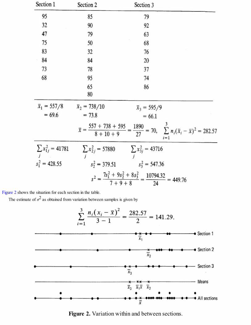
Figure 2 shows the situation for each section in the table.The estimate of σ2 as obtained from variation between samples is given by

Figure 2. Variation within and between sections.

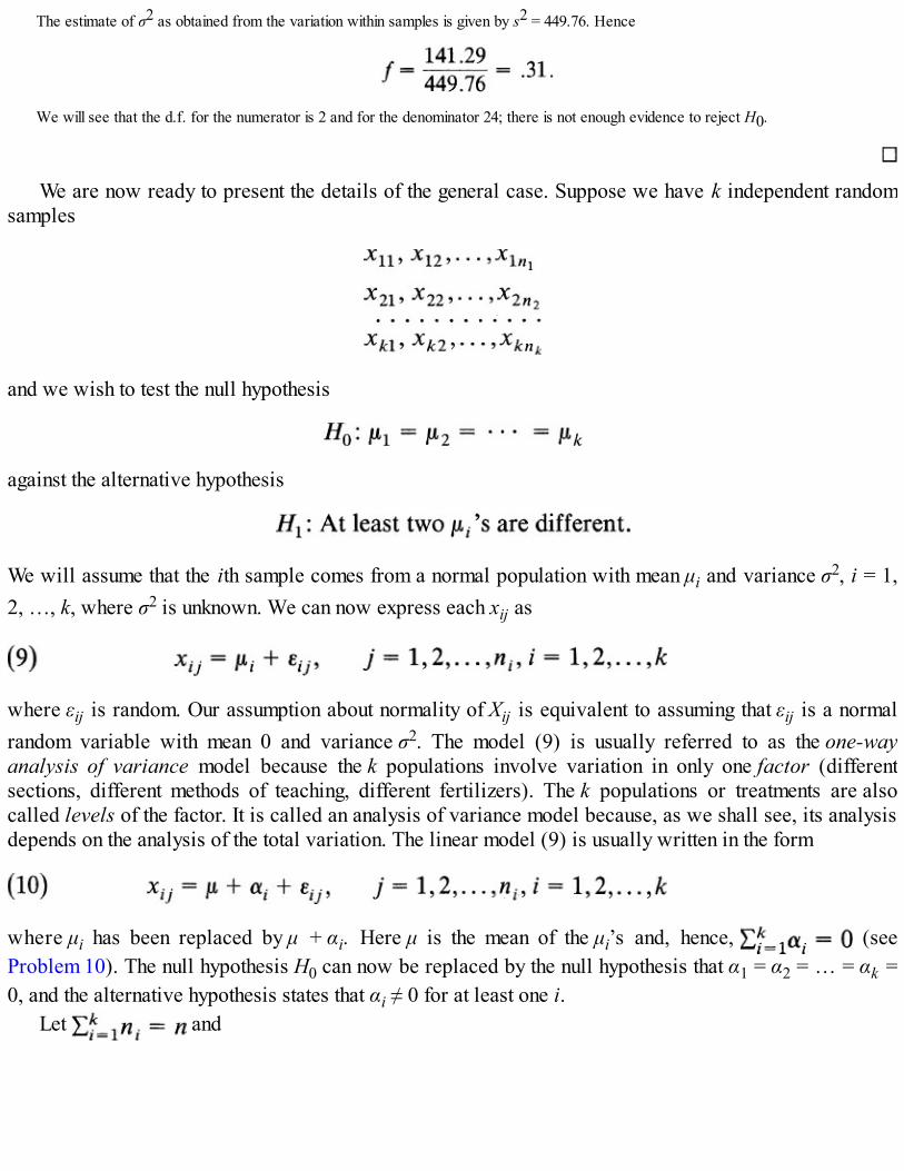
The estimate of σ2 as obtained from the variation within samples is given by s2 = 449.76. Hence

We will see that the d.f. for the numerator is 2 and for the denominator 24; there is not enough evidence to reject H0.

We are now ready to present the details of the general case. Suppose we have k independent randomsamples

and we wish to test the null hypothesis

against the alternative hypothesis

We will assume that the ith sample comes from a normal population with mean μi and variance σ2, i = 1,2, …, k, where σ2 is unknown. We can now express each xij as

where εij is random. Our assumption about normality of Xij is equivalent to assuming that εij is a normalrandom variable with mean 0 and variance σ2. The model (9) is usually referred to as the one-wayanalysis of variance model because the k populations involve variation in only one factor (differentsections, different methods of teaching, different fertilizers). The k populations or treatments are alsocalled levels of the factor. It is called an analysis of variance model because, as we shall see, its analysisdepends on the analysis of the total variation. The linear model (9) is usually written in the form

where μi has been replaced by μ + αi. Here μ is the mean of the μi’s and, hence, (seeProblem 10). The null hypothesis H0 can now be replaced by the null hypothesis that α1 = α2 = … = αk =0, and the alternative hypothesis states that αi ≠ 0 for at least one i.

Let and

and

We will compare two estimates of the variance σ2. One is based on the variation among the samplemeans and the other is based on the variation within the samples. First note that the total variation (TSS)is given by

so that

Writing Xij for the random variable that takes values xij we note also that

so that

is an unbiased estimate of σ2, under H0 as well as under H1 Next we have

where . It follows that

with equality if and only if μ1 = μ2 = ··· = μk. In particular,

is an unbiased estimate of σ2 under H0.Consider the ratio

of the two estimates of σ2. We note that the statistic F is an estimate of the ratio

In view of the law of large numbers when each ni is large, the ratio F in (14) is likely to be near the ratio

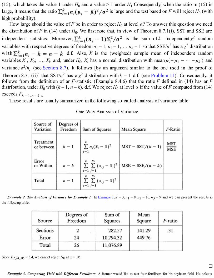
(15), which takes the value 1 under H0 and a value > 1 under H1 Consequently, when the ratio in (15) islarge, it means that the ratio is large and the test based on F will reject H0 (withhigh probability).

How large should the value of F be in order to reject H0 at level α? To answer this question we needthe distribution of F in (14) under H0. We first note that, in view of Theorem 8.7.1(i), SST and SSE areindependent statistics. Moreover, is the sum of k independent χ2 randomvariables with respective degrees of freedom n1 – 1, n2 – 1, … nk – 1 so that SSE/σ2 has a χ2 distributionw i th d.f. Also, X is the (weighted) sample mean of independent randomvariables X1, X2, …, Xk and, under H0, Xi has a normal distribution with mean μ(= μ1 = ··· = μk.) andvariance σ2/ni (see Section 8.7). It follows [by an argument similar to the one used in the proof ofTheorem 8.7.1(ii)] that SST/σ2 has a χ2 distribution with k – 1 d.f. (see Problem 11). Consequently, itfollows from the definition of an F-statistic (Example 8.4.6) that the ratio F defined in (14) has an Fdistribution, under H0 with (k – 1, n – k). d.f. We reject H0 at level α if the value of F computed from (14)exceeds Fk – 1, n – k , α.

These results are usually summarized in the following so-called analysis of variance table.

One-Way Analysis of Variance

Example 2. The Analysis of Variance for Example 1 . In Example 1, k = 3, n1 = 8, n2 = 10, n3 = 9 and we can present the results inthe following table.

Since F2,24,.05 = 3.4, we cannot reject H0 at α = .05.

Example 3. Comparing Yield with Different Fertilizers . A farmer would like to test four fertilizers for his soybean field. He selects

plots of the same size having similar soil, drainage, and exposure to the sun. He tries fertilizers A, B, C, and D respectively on 6, 8, 9 and 7 testplots with the following yields.

Fertilizer YieldA 47, 42, 43, 46, 44, 42B 51, 58, 62, 49, 53, 51, 50, 59C 37, 39, 41, 38, 39, 37, 42, 36, 40D 42, 43, 42, 45, 47, 50, 48

Is there significant difference in the average yieldsLet μA, μB, μC, μD be the mean yields. Then we wish to test H0: μA = μB = μC = μD against the alternative hypothesis that not all μ’s

are equal. We note that k = 4, n1 = 6, n2 = 8, n3 = 9, n4 = 7, and n = 30. We have

Hence

Analysis of Variance

Since F3,26,.05 = 2.89, we reject H0 at 5 percent level of significance and conclude that the fertilizers do not all have the same yield.

Remark 1. The F-test obtained here can be shown to be the likelihood ratio test. We asked students toderive the likelihood ratio test for the k = 3 case in Problem 11.4.10(ii).

Remark 2. The assumption σ1 = σ2 = ··· = σk that we made in this section can, be tested, for example,by using the likelihood ratio procedure [see Problem 11.4.10(i)]. We advise once more against the use ofa sequence of tests. The F-test that we developed in this section is robust in the sense that it is not toosensitive to departures from normality as well as from the assumption of equality of variances.

Remark 3. When the ni’s are large, one should avoid using the F-test. Indeed, when the ni’s are largethe quantity will be large even if the differences among the μi’s are small. Forsufficiently large values of ni’s the F-test will reject H0 (with high probability) even if the differencesamong the μi’s are practically negligible.

Remark 4. The case when we are not willing to assume that the Xij’s have a normal distribution butonly that they have a continuous distribution will be considered in Sections 13.5 and 13.6.

Remark 5. The one-way classification model of this section is also called a completely randomizeddesign. Once the n subjects have been chosen they are allocated to the k different treatments in acompletely random manner. Thus n1 subjects are randomly chosen from n and allocated to treatment 1,next n2 are randomly chosen from n – n1 remaining subjects and allocated to treatment 2, and so on.

Remark 6. The one-way analysis of variance model (10) is called a fixed effects model because it isassumed that the levels chosen for the analysis are the only ones considered relevant. If we replace thefixed αi’s in (10) by random variables Ai, we get the so-called random effects model. In a random effectsmodel we also need to make assumptions concerning the Ai’s. We will not consider such models in thistext.

Problems for Section 13.2

1. Five car models are chosen in a study to test the equality of average gasoline mileage per gallon that each model gives. Independentrandom samples of 5, 6, 4, 7, and 6 cars of each model were selected and each car was run on one gallon of gasoline until it ran out ofgas. The miles traveled (rounded off to the nearest integer) by each car are given below.

Model Distance Traveled (miles)A 18, 17, 18, 21, 19B 21, 24, 17, 23, 22, 23C 15, 14, 16, 15D 18, 20, 20, 24, 26, 23, 25E 17, 16, 18, 17, 15, 17

Is there sufficient evidence to suggest that the five models give different mpg?

2. In order to compare the effectiveness of four methods of teaching young children a computer programming language, independent randomsamples of sizes 4, 7, 6, and 8 are taken from large groups of children taught by these four methods, and their scores on a standardizedachievement test are recorded as follows:

Model ScoresA 75, 73, 68, 72B 84, 92, 84, 82, 87, 85, 87C 62, 65, 68, 67, 67, 66D 74, 76, 73, 72, 76, 74, 75, 79

Is there evidence to conclude that there is significant difference among the four methods of instruction?

3. Five cigarette manufacturers claim that their product has low tar content. Independent random samples of cigarettes are taken from eachmanufacturer and the following tar levels (in milligrams) are recorded.

Brand Tar Level (mg)A 4.2, 4.8, 4.6, 4.0, 4.4B 4.9, 4.8, 4.7, 5.0, 4.9, 5.2C 5.4, 5.3, 5.4, 5.2, 5.5D 5.8, 5.6, 5.5, 5.4, 5.6, 5.8E 5.9, 6.2, 6.2, 6.8, 6.4, 6.3

Can the differences among the sample means be attributed to chance?

4. Four brands of bacon are tested for fat contents with the following sample results.

Brand Fat Content(%)1 41, 42, 40, 44, 432 38, 34, 36, 37, 38, 363 42, 45, 48, 46, 47, 484 54, 52, 51, 52, 53

Is the difference among the mean fat contents significant at level .05?

5. There are three banks in Bowling Green, Ohio. Customers are randomly selected from the main branch of each bank and their waitingtimes before obtaining service from a teller are recorded as follows:

Bank Waiting Times (min.)HB 2.5, 3.0, 3.5, 6.0, 3.5, 4.5MA 4.5, 8.0, 6.5, 6.0, 7.5, 6.0, 7.5TT 2.5, 3.5, 4.0, 3.5, 2.5

Do the data indicate a significant difference among the mean waiting times at these banks?

6. The quantity of oxygen dissolved in water is used as a measure of water pollution. Samples are taken at four locations in a lake and thequantity of dissolved oxygen is recorded as follows (lower reading corresponds to greater pollution):

Location Quantity of Dissolved Oxygen (%)A 7.8, 6.4, 8.2, 6.9B 6.7, 6.8, 7.1, 6.9, 7.3C 7.2, 7.4, 6.9, 6.4, 6.5D 6.0, 7.4, 6.5, 6.9, 7.2, 6.8

Do the data indicate a significant difference in the average amount of dissolved oxygen for the four locations?

7. Four different brands of 9-volt batteries are to be compared to see if the mean life lengths are the same. Independent random sampleswere taken and the lifetimes of sample batteries were recorded (in hours) as follows:

Brand Life Length (hr.)A 42, 46, 43, 48, 47, 47B 54, 53, 50, 58, 55C 37, 35, 41, 32, 36, 37D 49, 48, 48, 50, 49

What is your conclusion?

8. A psychologist is interested in comparing the mean reaction time of five types of laboratory animals to a particular stimulus. She obtains thefollowing results:

Do the data indicate that the mean reaction times are significantly different at a 5 percent level of significance?

9. Show that

and hence that

Conclude that when H0: μ1 = μ2 is false (that is, when μ1 ≠ μ2 is true) the estimate SST of σ2 (with high probability) will exceed the

estimate S2 = SSE/(n1 + n2 – 2) of σ2.

10. Show that the model

can be written as

where

11*. Show that the statistic has a χ2 (k – 1) distribution under H0: μ1 = μ2 = ··· = μk = μ (unknown). {Hint:

. Use an argument similar to the oneused in the proof of Theorem 8.7.1(ii).}

12. Show that the F-test in one-way analysis of variance is equivalent to the test based on the statistic

13.3 MULTIPLE COMPARISON OF MEANS

In Example 13.2.3 the null hypothesis, that the four fertilizers have the same mean yield, was rejected.From the farmer’s point of view, the problems is not really solved. In order to determine which fertilizerto buy he needs to do a cost analysis and for that purpose he needs to be able to rank, if possible, the fourfertilizers according to their average yield. The data of Example 13.2.3 suggest that μB > μA = μD > μC.What evidence does the data offer to make this assertion? In other words, with what degree of confidencecan we assert that fertilizer B produces the largest average yield whereas the fertilizer C produces theleast average yield?

More formally, suppose the F test in a one-way analysis of variance rejects the null hypothesis H0: μ1

= μ2 = ··· = μk. How do we obtain simultaneous confidence intervals for the differences μi – μj for eachpair of population means (μi, μj) at level 1 – α? Several such multiple comparison procedures areavailable. We will only consider the following method, due to Scheffé:

In random sampling from k normal populations with common (unknown) variance, the probability is 1 – α that

holds for all c1, c2, …, ck such that . Here

We will not attempt to prove this result here. It should be noted that the result holds for allcomparisons simultaneously. It should not be surprising, therefore, to find that the length of aconfidence interval for a particular linear function such as μ1 – μ2 obtained by this method is much largerthan the length of a 1 – α level confidence interval for μ1 – μ2 based on the t-statistic (as obtained inSection 8.7).

We note that in view of (13.2.12),

in the notation of Section 13.2, so that we have

In the particular case when ci = 1, cj = –1 and other c’s are zero we have

Example 1. Comparing Mean Yields with Different Fertilizers (Example 13.2.3 continued). In Example 13.2.3 we obtained thefollowing sample results.

Also, MSE = 277.87/26 = 10.69 and F3, 26, .05 = 2.89. Then

The following table gives the six simultaneous confidence intervals for μi – μj, i < j, i, j = 1, 2, 3, 4. (For convenience, we have written i = 1for A, i = 2, for B, and so on.)

The confidence intervals that do not contain zero are the ones for μA – μB, μB – μC, μB – μD and μC – μD. Clearly we can assert with 95percent confidence that

and

Thus

Consequently, with 95 percent confidence we can assert that fertilizer B results in the largest mean yield. It is not possible to make anyassertion concerning the relative order of μA, μC and μD (except that μD > μC) since μA and μC, and μA and μD are not significantlydifferent.

On the other hand, if our objective is to compare only μA and μC, then we can use a 95 percent confidence interval based on the t-statistic. This confidence interval is given by

where

For 13 d.f., t13, .025 = 2.160 and the confidence interval is given by

The length of this confidence interval is smaller than the length of the interval obtained by Scheffé’s method. This confidence interval,however, is a statement concerning μA – μC alone, whereas Scheffé’s method makes a statement simultaneously concerning all the sixpossible differences.

Example 2. Comparing the Average Number of Defects in Automobiles . An automobile assembly plant assembles several models. Inorder to investigate if more expensive models receive greater care than the less expensive models, several cars of the three models assembledat this plant are tested for defects with the following results. (Model A cars are the most expensive and Model C cars are the least expensive).

Model Number of DefectsA 5, 4, 6, 6, 7B 7, 8, 6, 7, 6, 5C 9, 7, 8, 9, 10, 11, 10, 10

Writing i = 1, 2, 3 respectively for A, B, and C we see that

Analysis of Variance

Since F2, 16, .05 = 3.63 we have to reject H0: μA = μB = μC at level α = .05 and conclude that the mean number of defects for the modelsare different.

Let us now apply Scheffé’s method to investigate which differences are significantly different from zero. We note that

The following table gives the confidence intervals for μi, – μj, i ≠ j

Mean Difference Lower Limit Upper LimitμA – μB –2.8 1.0μA – μC –5.5 –1.8μB – μC –4.5 –1.0

Since the confidence intervals for μA – μC and μB – μC are both to the left of zero, we can assert with 95 percent confidence that

so that the average number of defects for the least expensive model is the greatest of the three models.

Problems for Section 13.3

1. For the data on distance traveled in miles per gallon of gasoline for the five models of automobiles in Problem 13.2.1, the sample results areas follows:

Find simultaneous confidence intervals (for the differences between the means) at level .95. Which means are significantly different atlevel .05?

2. The following table gives the relevant sample statistics for the data of Problem 13.2.2.

Investigate significant differences in the true mean scores between different methods at level .05.

3. The following table gives the relevant sample statistics for the data on fat contents in four brands of bacon of Problem 13.2.4.

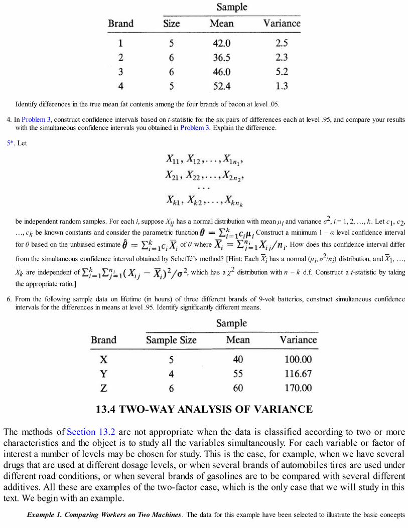
Identify differences in the true mean fat contents among the four brands of bacon at level .05.

4. In Problem 3, construct confidence intervals based on t-statistic for the six pairs of differences each at level .95, and compare your resultswith the simultaneous confidence intervals you obtained in Problem 3. Explain the difference.

5*. Let

be independent random samples. For each i, suppose Xij has a normal distribution with mean μi and variance σ2, i = 1, 2, …, k . Let c1, c2,…, ck be known constants and consider the parametric function Construct a minimum 1 – α level confidence interval

for θ based on the unbiased estimate of θ where . How does this confidence interval differ

from the simultaneous confidence interval obtained by Scheffé’s method? [Hint: Each Xi has a normal (μi, σ2/ni) distribution, and X1, …,

Xk are independent of , which has a χ2 distribution with n – k d.f. Construct a t-statistic by takingthe appropriate ratio.]

6. From the following sample data on lifetime (in hours) of three different brands of 9-volt batteries, construct simultaneous confidenceintervals for the differences in means at level .95. Identify significantly different means.

13.4 TWO-WAY ANALYSIS OF VARIANCE

The methods of Section 13.2 are not appropriate when the data is classified according to two or morecharacteristics and the object is to study all the variables simultaneously. For each variable or factor ofinterest a number of levels may be chosen for study. This is the case, for example, when we have severaldrugs that are used at different dosage levels, or when several brands of automobiles tires are used underdifferent road conditions, or when several brands of gasolines are to be compared with several differentadditives. All these are examples of the two-factor case, which is the only case that we will study in thistext. We begin with an example.

Example 1. Comparing Workers on Two Machines . The data for this example have been selected to illustrate the basic concepts

involved in a two-factor analysis of variance.Suppose we wish to test whether there are any differences in two different machines that were used by two workers. Suppose,

further, that four weeks are selected for this study, each week consisting of five working days. During the first and second weeks worker1 is used and during third and fourth weeks worker 2 is used. Machine 1 is used during the first and third weeks and machine 2 is usedduring the second and fourth weeks. Suppose other conditions of work are identical. The data in Table 1 represent the number of unitsproduced per day.

It would be inappropriate to apply a one-way analysis of variance to this data. There are two factors to be considered here. One is theeffect of the workers and the other is the effect of the machines. There may also be an effect of the interaction between worker andmachine. There are several questions of interest that we would like to answer. Do variations in the machines or in the worker affect theproduction? That is, which of these two factors makes a significant contribution to the number of units produced per day? Is a change inthe number of units of production that can be attributed to a change in the machines the same for the two workers?

In order to show the interdependence between the two factors, we exhibit the data in Table 2.

TABLE 1. Number of Units Produced per Day

Week Number of Units Produced1 69, 68, 72, 74, 752 95, 98, 100, 96, 973 81, 88, 84, 87, 884 105, 110, 107, 112, 118

TABLE 2

Here we have two levels of factor A, workers 1 and 2, and two levels of factor B, machines 1 and 2. The four subsquares into whichTable 2 is subdivided are usually referred to as cells. Let us call the cell for which factor A is at level i and factor B at level j, the (i, j) thcell, i = 1, 2; j = 1, 2. Each cell in Table 2 has five observations, all taken at the same set of factor levels. We assume that theobservations in the (i, j)th cell are a random sample from a normal population with mean μij and variance σ2, both unknown.

The main features of a two-way analysis of variance are that:(i) it allows us to compare the effects of two variables (factors),(ii) it allows us to study the interaction effects, if any, of the two variables.

In order to study the simultaneous but separate effects of factors A and B one performs two F-tests, one for the worker “main”effect and another for the machine “main” effect. The most interesting aspect of the two-way analysis of variance (and also the mostdifficult to explain) is its ability to identify the interaction effects. It is easier to define “no interaction.” We say that there are nointeractions between two factors if the presence or absence of factor A has no effect on Factor B, and conversely. In that case theamount by which factor A raises the mean number of units produced is the same regardless of the level of Factor B, and conversely.Thus the cell mean when there are no interactions are as follows.

If we write μ12 = μ11 + β, we get the following table of means for the “no interaction” case.

Thus “no interaction” means that the effects of the two factors are additive in the following sense. If a change in factor A by itselfproduces a change α in cell means, and a change in factor B by itself produces a change β in cell means, then changes in both factorsproduce a change of α + β in the cell means. This can be illustrated with the help of a diagram. Suppose the mean number of unitsproduced per day are as follows.

Then μ11 = 72, α = 13, β = 25 and the two factors are additive. We can plot the means as in Figure 1. We see that there is no crossingover of the line segments depicting the two levels of each factor.

In order to illustrate an interaction effect, suppose the table of means was as follows.

Now we have two main effects (actually only one—see Problem 2) as well as an interaction effect. Both workers produce more units onMachine 2. Worker 1 produces less than worker 2 on Machine 2 but the reverse is true on Machine 1. This is seen more clearly in Figure2.

In the case of additive factors, the graphs of cell means will look like those in Figure 1 (parallel line segments) and in the case ofinteraction the graphs will look like those in Figure 2 where the line segments cross over.

In practice one does not know the μij’s. In that case one plots the corresponding sample means. The interpretation is the same. Ifthere is little or no crossing over of line segments, it indicates that the two factors are additive. Otherwise there is also interaction betweenthe two factors.

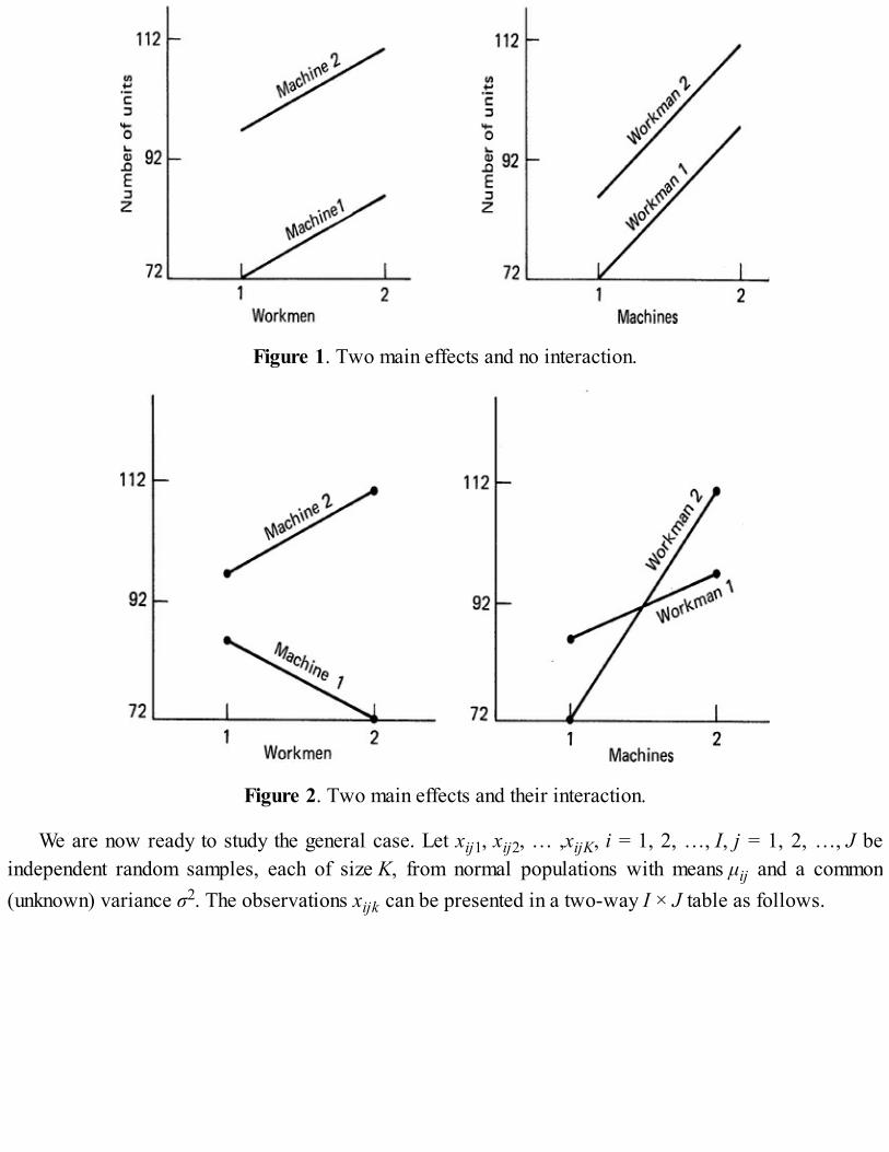
Figure 1. Two main effects and no interaction.

Figure 2. Two main effects and their interaction.

We are now ready to study the general case. Let xij1, xij2, … ,xijK, i = 1, 2, …, I, j = 1, 2, …, J beindependent random samples, each of size K, from normal populations with means μij and a common(unknown) variance σ2. The observations xijk can be presented in a two-way I × J table as follows.

Thus xijk is the kth observation, k = 1, 2, …, K in the (i, j)th cell; that is, it is the kth observation whenfactor A is held at level i and factor B is held at level j. Let I ≥ 2, J ≥ 2, and K ≥ 2. Set

Let us call

and

Thus

We note that

As usual let Xijk denote the random variable, which takes values xijk, k = 1, 2, …, K. Then (1) can berewritten as

for k = 1, 2, …, K. We write

where εijk, for k = 1, 2, …,K, are independent and identically distributed normal random variables withmean 0 and variance σ2. Thus Xijk for k = 1, 2, …, K are independent and identically distributed normalrandom variables with mean μij and variance σ2. Equation (3) is usually referred to as the (linear) two-way analysis of variance model.

The object of the analysis of variance is to test the following different hypotheses:

HA: α1 = β2 = ··· = αI = 0 (no effect due to factor A)

HB: β1 = β2 = ··· = βJ = 0 (no effect due to factor B)HAB: γij = 0 for all i, j, i = 1, 2, …, I, j = 1, 2, …, J (no interaction effects)

The null hypothesis HAB simply states that the effects of factors A and B are additive. The procedure forsimultaneously testing HA, HB, and HAB is the same as in the one-way analysis of variance. We partitionthe total variation into four parts, one part attributable to factor A, the second part attributable to factor B,the third part attributable to interaction between factors A and B, and the fourth (remaining) partattributable to random error. Comparisons of each of the first three parts to the random error part allowsus to test the three null hypotheses HA, HB, and HAB. We define

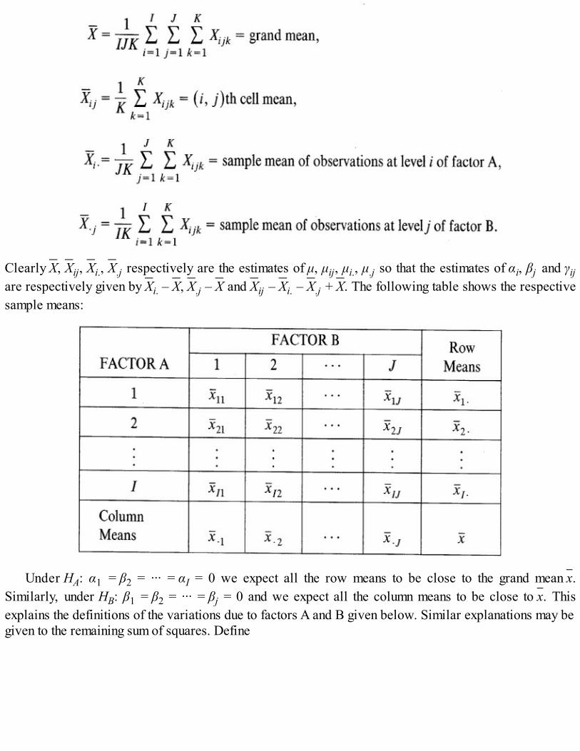
Clearly X, Xij, Xi., X.j respectively are the estimates of μ, μij, μi., μ.j so that the estimates of αi, βj and γijare respectively given by Xi. – X, X.j – X and Xij – Xi. – X.j + X. The following table shows the respectivesample means:

Under HA: α1 = β2 = ··· = αI = 0 we expect all the row means to be close to the grand mean x.Similarly, under HB: β1 = β2 = ··· = βj = 0 and we expect all the column means to be close to x. Thisexplains the definitions of the variations due to factors A and B given below. Similar explanations may begiven to the remaining sum of squares. Define

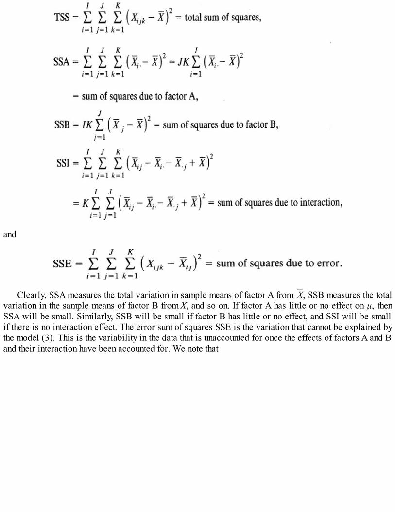
and

Clearly, SSA measures the total variation in sample means of factor A from X, SSB measures the totalvariation in the sample means of factor B from X, and so on. If factor A has little or no effect on μ, thenSSA will be small. Similarly, SSB will be small if factor B has little or no effect, and SSI will be smallif there is no interaction effect. The error sum of squares SSE is the variation that cannot be explained bythe model (3). This is the variability in the data that is unaccounted for once the effects of factors A and Band their interaction have been accounted for. We note that

so that on expanding we get

Relation (4) holds since all the six product terms vanish. For example,

and so on.Exactly as in the one-way analysis of variance we can use each of the four sums of squares on the

right side of (4) to estimate σ2. Thus, we can show (Problem 1) that

and

where MSA is called the mean sum of squares due to factor A, MSB the mean sum of squares due tofactor B, and so on. Under HA, (MSA) = σ2; under HB, (MSB) = σ2, and under HAB, (MSI) = μ2.Moreover, if HA is false then

Now the ratio

is an estimate of the ratio

If HA is false then FA will tend to be large. It is possible to show by using the normal theory of Section 8.7(exactly as in the one-way analysis of variance case) that FA has an F(I – 1, IJ(K – 1)) distribution. Hencewe reject HA at level α if

Similar arguments lead to the following level α tests of HB and HAB:

These results can now be summarized in the following two-way analysis of variance table:

Two-Way Analysis of Variance

The computation of SSA, SSB, SST, and SSE can be simplified be expanding each sum of squares.Thus

For convenience, we write

Then

Similarly,

and by subtraction

Example 2. Example 1 Revisited. From Table 2 in Example 1 we get the following tables of sample sums and sample means

If the sample means are plotted as in Example 1, the plots will look like Figure 1. The line segments will not be parallel but almostparallel, the best that one can expect from the sample data. This suggests that there is no interaction between the factors and one coulduse the additive model

instead of the model (3). From the table for sample totals we have

Also

Then

so that

These results are summarized in the following analysis of variance table.

Analysis of Variance for Table 2

We note that F1, 16, .01 = 8.53, F1, 16, .05 = 4.49 so that both HA and HB are rejected, whereas HAB cannot be rejected. Thus thereis an effect on production that can be attributed to differences in workers as well as to differences in machines, but there is no interactionbetween the workers and the machines.

Example 3. Variety of Wheat vs. Location . Three varieties of wheat were grown at three different locations. A sample of eachvariety was taken from each location and milled into flour. Three loaves of bread were baked from each sample of flour. The followingtable gives the volumes of loaves measured in standard units.

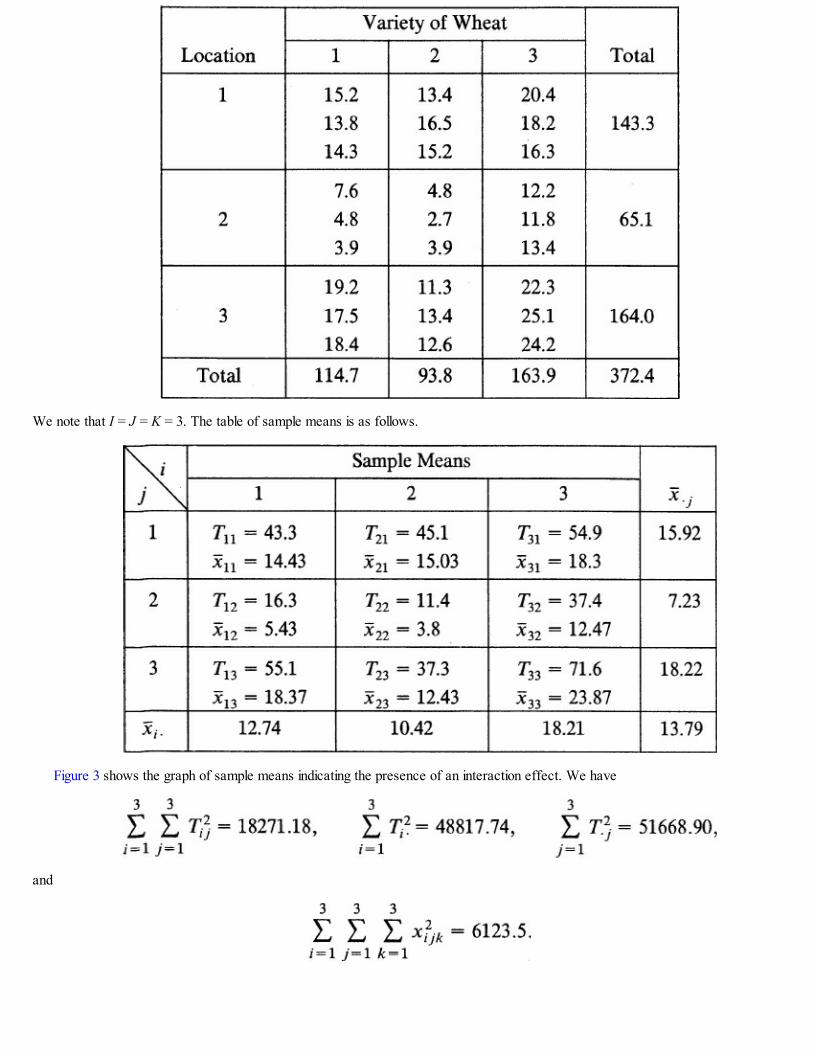
We note that I = J = K = 3. The table of sample means is as follows.

Figure 3 shows the graph of sample means indicating the presence of an interaction effect. We have

and

Figure 3. Interaction between variety and location.

Thus

and

Since F2, 18, .01 = 6.01, and F4, 18, .01 = 4.58 we have to reject HA, HB, and HAB at level α = .01 and conclude that both thelocation of the plot as well as the variety of wheat used affect the volume of loaves baked. Moreover, the volume is also affected by theinteraction between the location and the variety of wheat used.

13.4.1 Randomized Block Design

Suppose I ≥ 2, J ≥ 2, and K = 1 in a two-way analysis of variance so that we have exactly oneobservation per cell. In that case, since xijk = xij for all i, j and wecannot test for interaction between the two factors. Suppose the effects of the two factors are additive (theinteractions γij are all zero). In that case,

and we can use MSI as the denominator of the F-ratio for testing HA or HB. The analysis of variance tablethen reduces to the following table.

Two-way Analysis of Variance—One Observation per Cell

In many practical applications, an artifical factor B is created to reduce variability. Suppose we haven = IJ experimental units available which can be divided into J homogeneous groups called blocks. Eachblock consists of I units. Within each homogeneous block, the I treatments are assigned randomly to the Iunits in the block. This arrangement of n = IJ units in J blocks is called a randomized (complete) blockdesign. We recall (Remark 13.2.5) that in a completely randomized design, on the other hand, the Itreatments are randomly allocated to n = IJ experimental units such that each treatment appears in J units(one can have repetitions of the I treatments).

The blocks in a randomized block design can be groups of plots of land, groups of animals of the sametype (cows or rats or pigs), groups of locations, groups of students, and so on.

Even though the data in a randomized block design is classified according to two factors it does notnecessarily follow that we are always interested in analyzing the differences among the block means. Aspointed out earlier, blocks are introduced in order to eliminate heterogeneity caused by some extraneousfactor; the object being to have experimental units that are as nearly identical as possible.

Example 45. Weight Gains by Swines . A swine-feeding experiment involving three different rations, A, B, and C, was laid out in arandomized block design using 15 animals in five groups of three each. The grouping was done on the basis of initial weight and Utter.The litters are the blocks, since we expect the animals to be homogeneous within litter. The following table, arranged in five blocks, showsthe weight gains in pounds. The ration fed is shown along with the observation.

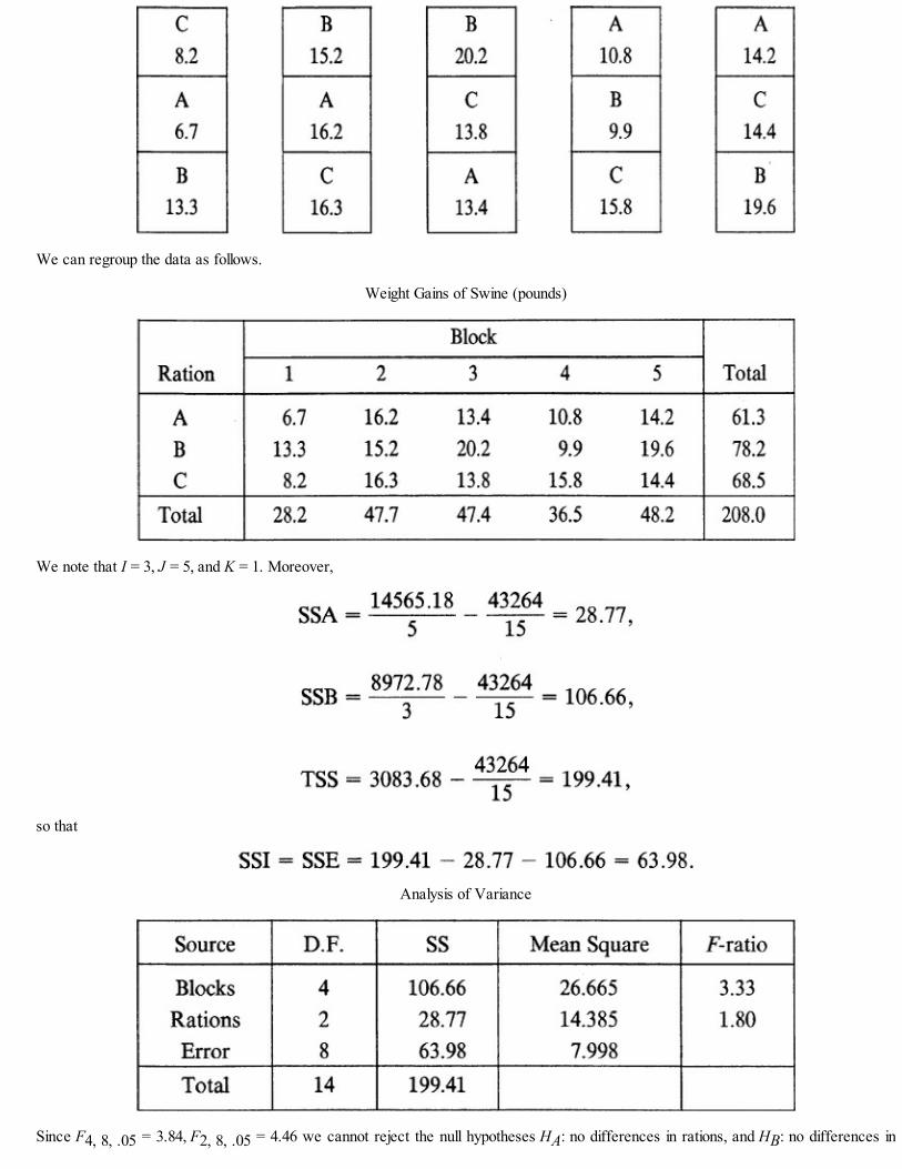
We can regroup the data as follows.

Weight Gains of Swine (pounds)

We note that I = 3, J = 5, and K = 1. Moreover,

so that

Analysis of Variance

Since F4, 8, .05 = 3.84, F2, 8, .05 = 4.46 we cannot reject the null hypotheses HA: no differences in rations, and HB: no differences in

litters.

13.4.2 Multiple Comparisons in Two-Way Analysis of Variance

Whenever either HA or HB is rejected (and HAB is not rejected), it is of interest to know the significantlydifferent levels of the factor under study. The procedure is the same as in the one-way analysis ofvariance. In order to compare levels of factor A we use the simultaneous confidence intervals given by

where

and

Example 5. Comparing Four Brands of Tires . In an experiment to compare tread wear of four different brands of tires after 20,000miles of driving, a randomized block design was used with four cars serving as the four blocks. Each of the four sets of automobile tires ismounted in a random order on each car and then the car is run for 20,000 miles. The following table gives the tread wear (in units of 0.001inch).

Thus

and

so that

The following table gives the two-way analysis of variance.

Since F3, 9, .01 = 6.99 we reject the null hypothesis HA that the four brands of tires show the same mean tread wear after 20,000 miles ofdriving. Although the object was to compare differences in brands of tires, we can also test the null hypothesis HB that average tread wear forall four cars is the same. We note that HB is also rejected at 1 percent level.

Let us now compare the six pairs of brand means by using Scheffé’s multiple comparison method. Since I = J = 4 and MSE = .694, wehave with α = .05

so that

We note that

so that at an overall level .05, the mean for Brand C is significantly different from those for Brands A, B, and D. Since the Brand C mean isthe highest, this means that Brand C exhibits the greatest tread wear. A similar comparison may be made for the car means if so desired.

Problems for Section 13.4

1. Recalling that

for i = 1, 2, …, I, j = 1, 2, …, J, k = 1, 2, …, K where and the definitions ofX, Xi., X.j, and Xij show that

Hence show that

[Hint: Prove and use the relations Xi. = μ + α1 + (JK)–1εi. where , and so on, and

, and so on.]

2. Let K = 2, I = 2, and J = 2 and consider the model in equation (2),

where

Show that

In particular, consider the table of means:

so that μ11 = 85, μ12 = 97, μ21 = 72, and μ22 = 110. Show that μ = 91, λ11 = 6.5, β1 = –12.5, and α1 = 0.

3. To test the effectiveness of three teaching methods, three instructors were randomly assigned 15 students each. The students were thenrandomly assigned to the different teaching methods (five to each method) and were taught exactly the same material. At the conclusionof the experiment, the same examination was administered to all the students with the following results.

(i) Assuming that the two main effects are additive, perform the two-way analysis of variance to test the hypotheses that the threemethods are equally effective and that the three instructors are equally effective.

(ii) Construct the two-way analysis of variance table assuming interaction between the instructor and the teaching method. Test the threehypotheses HA, HB, and HAB.

4. The following data represent the number of units produced by three workers, each working on the same machine for four different days.

Test whether:(i) The differences among the machines are significant.(ii) The differences among the workmen are significant.(iii) The interactions are significant.Take α = .05.

5. The following table shows the yield (pounds per plot) of four varieties of wheat, obtained with three different kinds of fertilizers.

Test the hypotheses that the four varieties of wheat yield the same average yield and that the three fertilizers are equally effective.

6. In an experiment to determine whether four different makes of automobiles average the same gasoline mileage, a random sample of twocars of each make was taken from each of four cities. Each car was then test run on five gallons of gasoline of the same brand. Thefollowing table gives the number of miles traveled.

Construct the analysis of variance table. Test the hypotheses of no automobile effect, no city effect, and no interactions. Use α = .05.

7. In a field trial four strains of wheat are planted in four blocks. The treatments (strains of wheat) are assigned to the four plots into whicheach block is divided at random. The following table shows the yield (in pounds per plot) by block.

(i) Construct the analysis of variance table for this randomized block design experiment.(ii) Test the hypothesis that there are no differences among the strains of wheat.(iii) Construct .95 level simultaneous confidence intervals for differences among mean yields of the four strains of wheat. Identify

significantly different strains of wheat.

8. An experiment is designed to test for differences in weight gains for steers produced by five different rations. Fifteen steers are allocatedto three blocks on the basis of their weight at the start of the experiment. The five rations (treatments) are assigned at random to the fivesteers within each block. The following data were obtained.

Weight Gains of Steers (pounds)

Construct the two-way analysis of variance table and test the hypothesis that there are no differences among the five rations in producingweight gains for steers. Identify significantly different rations by using multiple comparisons. Use α = .05.

9. In Problem 6 construct simultaneous confidence intervals at overall level .95 for differences among the means for the automobiles. Identifysignificantly different automobiles.

10. In Problem 3 construct simultaneous confidence intervals at overall level .95 for differences among the means of the three teachingmethods.

11. The following data show the pulse rates of 10 subjects recorded before and again 90 minutes after the administration of a particular drug.

(i) Apply Student’s t-test to test the null hypothesis that the mean pulse rates before and after are the same.(ii) Perform the two-way analysis of variance by using each subject as a block. Compare your result to that of part (i). (This is the data

on the first 10 subjects of Problem 8.7.11.)

13.5 TESTING EQUALITY IN k-INDEPENDENT SAMPLES: NONNORMALCASE

In Sections 13.2 and 13.3 we considered the problem of testing the null hypothesis

based on k-independent random samples from normal distributions with common unknown variance σ2.We now drop the assumption that the Fi’s are normal distribution functions and assume only that each Fi isa continuous distribution function.

In Section 12.2 we showed how the χ2 test for homogeneity of k proportions can be adapted to testequality of k distributions when the sample sizes are large. The median test of Section 6.4 can also beextended to test the equality of k distributions.

13.5.1 The Extended Median Test

Suppose we have k-independent random samples of sizes n1, n2, …, nk from respective distributionfunctions F1, F2, …, Fk that are assumed to be continuous. The null hypothesis of interest is that alldistributions have the same (unknown) median.

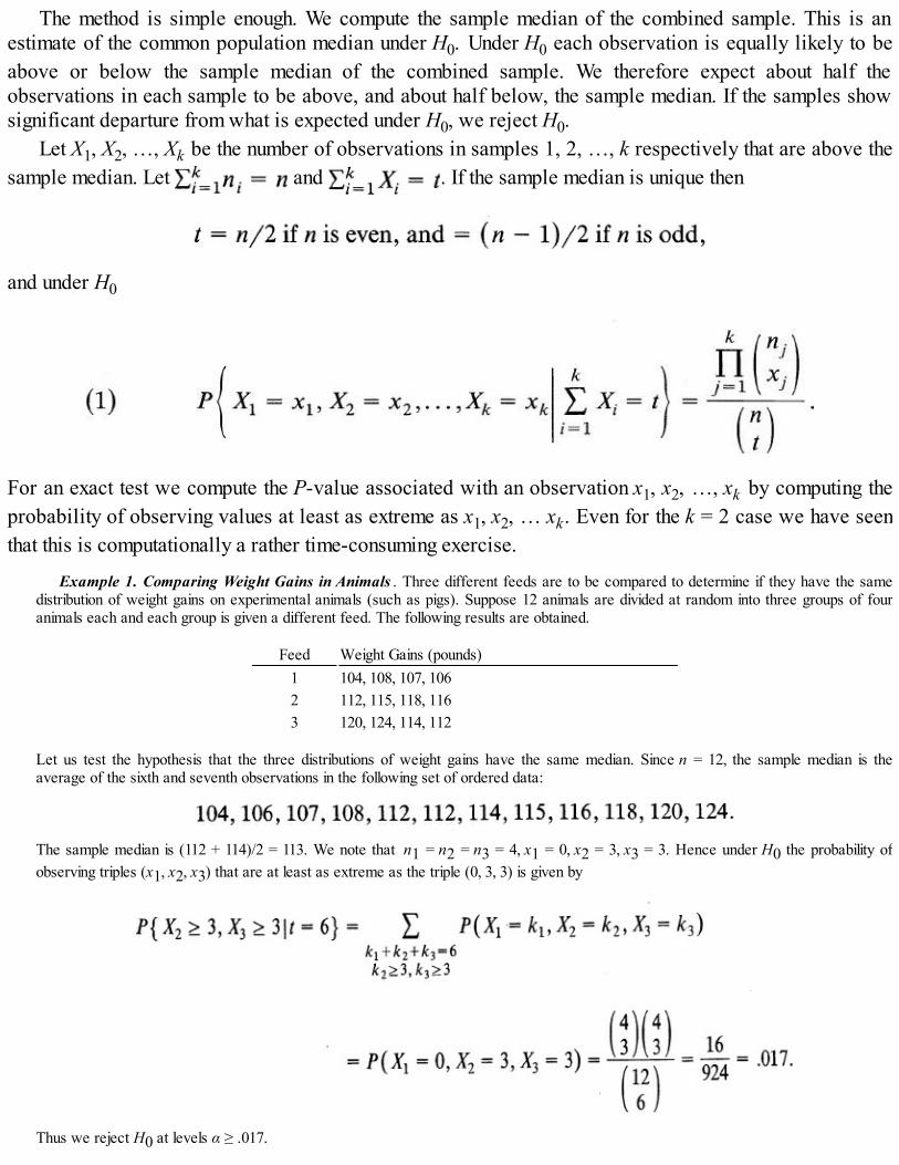
The method is simple enough. We compute the sample median of the combined sample. This is anestimate of the common population median under H0. Under H0 each observation is equally likely to beabove or below the sample median of the combined sample. We therefore expect about half theobservations in each sample to be above, and about half below, the sample median. If the samples showsignificant departure from what is expected under H0, we reject H0.

Let X1, X2, …, Xk be the number of observations in samples 1, 2, …, k respectively that are above thesample median. Let and . If the sample median is unique then

and under H0

For an exact test we compute the P-value associated with an observation x1, x2, …, xk by computing theprobability of observing values at least as extreme as x1, x2, … xk. Even for the k = 2 case we have seenthat this is computationally a rather time-consuming exercise.

Example 1. Comparing Weight Gains in Animals . Three different feeds are to be compared to determine if they have the samedistribution of weight gains on experimental animals (such as pigs). Suppose 12 animals are divided at random into three groups of fouranimals each and each group is given a different feed. The following results are obtained.

Feed Weight Gains (pounds)1 104, 108, 107, 1062 112, 115, 118, 1163 120, 124, 114, 112

Let us test the hypothesis that the three distributions of weight gains have the same median. Since n = 12, the sample median is theaverage of the sixth and seventh observations in the following set of ordered data:

The sample median is (112 + 114)/2 = 113. We note that n1 = n2 = n3 = 4, x1 = 0, x2 = 3, x3 = 3. Hence under H0 the probability ofobserving triples (x1, x2, x3) that are at least as extreme as the triple (0, 3, 3) is given by

Thus we reject H0 at levels α ≥ .017.

Let us now assume that the distributions of weight gains are normal and apply the one-way analysis of variance to the same data. Wehave

and

Analysis of Variance

For 2 and 9 d.f. we have F2, 9, .01 = 8.02 and we reject H0 at level α = .01. The result is the same although the normal theory test is ableto detect the difference among means even at the 1 percent percent level. This is to be expected. Actually F2, 9, .005 = 10.1 so that wereject H0 even at level .005.

When n is moderately large (n ≥ 25) and each ni is not too small (ni ≥ 5) we can apply the χ2

goodness of fit test, which is considerably simpler. Let us first settle the question of ties which,theoretically at least, occur with probability zero. In practice, several observations may be tied at thesample median. If the number of observations is large and there are only a few ties, one can drop the tiedobservations from consideration. However, we will adopt the following procedure. We will count thetied observations as being below the median. Accordingly, we replace each observation by the symbol aif it is above the sample median and by the symbol b otherwise. The resulting data can now be put into a 2× k contingency table as follows.

Let Under H0 we expect nit/n observations in the ith sample to be above the median andni(n – t)/n observations to be below the median. The statistic

has a χ2 distribution with

since we have estimated k parameters. We reject H0 at level (approximately) α if q0, the computed valueof Q, is ≤ χ2

k–1, α.

Example 2. Comparing Three Laboratories. In a study to ascertain whether or not three laboratories give essentially the sameresults, on the average, random samples of the same chemical mixture are sent to each laboratory for chemical analysis. The laboratoriesare asked to identify the percentage of chemical A in each sample.

Laboratory Percentage of Chemical A1 34.3, 32.4, 33.8, 35.6, 32.3, 34.5, 35.4, 33.92 36.4, 35.8, 37.2, 34.5, 36.1, 34.8, 35.6, 36.2, 36.43 35.3, 34.9, 35.1, 35.8, 36.1, 35.2, 35.8, 33.9

Since there are 25 observations in the pooled sample, the sample median is the 13th observation in the ordered arrangement. It is easy tosee that the sample median if 35.3. The frequency counts of the number of observations below and above the median are as follows:

Then

Since d.f. = k – 1 = 3 – 1 = 2, we see that the P-value satisfies

We can therefore reject H0 that the three medians are the same at level α = .1 but not at level α = .05. The evidence in favor of H0 thatthe data offer is not very strong.

We leave the reader to show that the one-way analysis of variance yields the following results.

For (2,22) d.f. the F value 8.57 is significant even at .005 level.

13.5.2 The Kruskal–Wallis Test: Nonparametric One-way Analysis of Variance

The median test loses information since it compares each observation to the sample median. It does notuse any information on the relative magnitude of each observation when compared with every otherobservation in the combined sample. The Kruskal–Wallis test effects this comparison by replacing eachobservation by its rank in the pooled sample. The smallest observation is replaced by its rank 1, the nextsmallest by rank 2, and so on, the largest by its rank n. Since the test is an extension of the Mann–Whitney–Wilcoxon test (just as the one-way analysis of variance F-test is an extension of the two-samplet-test), it is instructive to analyze the Mann–Whitney–Wilcoxon test a little more carefully. Let

and

The Mann–Whitney–Wilcoxon test of F1 = F2 is based on the statistic R1 (see Section 11.6.1). For largen1, n2 we know that

has approximately a standard normal distribution, so that

has approximately a χ2(1) distribution. The first thing to note is that since R2 = [n(n + 1)/2] – R1 we canrewrite (after some simple algebra) Z2 as

We note that Ri/ni is the mean rank of the ith sample, whereas (n + 1)/2 is the mean rank of the combinedsample. Thus Z2 is essentially the weighted sum of squares of deviations of each sample mean rank fromthe combined sample mean rank. Under H0, we have essentially one sample of n observations and weexpect the sum of the ranks n(n + 1)/2 to be divided proportionally among the two samples according totheir size. Thus statistic Z2 makes good sense to consider even when k ≥ 3. Accordingly, we define

This is the Kruskal–Wallis statistic. The larger the H the larger the disparity between the sample meanranks and the grand mean rank so that the rejection region is of the form H ≥ c.

The alert reader will notice that the quantity is the sum ofsquares due to treatments (SST) in the one-way analysis of variance carried out with each Xij replaced byits rank. Then why don’t we have MSE as the divisor? The answer is that the F-test is equivalent to thetest based on the ratio (Problem 13.2.12)

When each Xij is replaced by its rank, the denominator, which is the total sum of squares (TSS), is givenby

It follows that the test based on H is equivalent to the test based on the F-ratio (when each Xij is replacedby its rank).

It is easy to show (Problem 8) that a computationally more convenient form of H given in (6) is thefollowing

The null distribution of H for k = 3 and ni ≤ 5 is extensively tabulated.† For values of ni that are nottoo small, the null distribution of H may be approximated by the χ2 (k – 1) distribution. We will use the χ2

approximation whenever each ni > 5.When ties occur, we assign average rank to the tied observations. This does not affect the value of H

when ties occur within the same sample. When ties occur across samples and the number of ties is small,we use the same test and the same distribution. When the number of ties is large it is possible to use acorrection for ties, but we will not give this correction here.‡

Example 3. Comparing Weight Gains in Animals ( Example 1). For the data on weight gains of Example 1 let us assign ranks toeach observation in the combined sample. The following table gives the ranks and the rank sums Ri.

Feed

1 2 31 5.5 114 8 123 10 72 9 5.510 32.5 35.5

Then

For k = 3, n1 = n2 = n3 = 4 we see from the table cited above that PH0(H ≥ 7.5385) = .011 and PH0

(H ≥ 5.6923) = .049 so that .011 <PH0

(H ≥ 7.47) < .049. In fact, the exact probability is closer to .011 than to .049. In any event we have to reject the null hypothesis of theequality of distributions at level .05.

Example 4. Comparing Three Laboratories (Example 2). Let us order the 25 observations in increasing order of magnitude andassign ranks from 1 to 25. Tied observations are assigned average rank.

For convenience we rearrange the data in the following table.

Rank of Xij in Laboratory

1 2 36 23.5 132 18 103 25 11

15.5 7.5 181 22.5 20.5

7.5 9 1214 15.5 184.5 22 4.5

23.5Total 53.5 164.5 107.0

Thus

For 3 – 1 = 2 d.f. we note that

so that the Kruskal–Wallis test does better than the median test but somewhat worse than the F-test. This is to be expected, since F testuses more information whereas the median test loses information contained in the data.

13.5.3 Multiple Comparisons

In Example 4, the Kruskal–Wallis test rejects the equality of three medians so that we conclude that thethree distributions are not the same. Often we wish to identify significantly different medians. As pointedout in Section 13.3, since the object is to obtain simultaneous confidence intervals, pairwise comparisonsusing the Mann–Whitney–Wilcoxon test are not appropriate.

We will follow the procedure proposed by Dunn. Let Ri = Ri/ni be the sample mean of ranks assignedto the ith sample. Then

where p = α/k(k – 1) and zp is the quantile of order 1 – p under the standard normal distribution.

Example 5. Significantly Different Laboratories in Example 4. In Example 4, n1 = 8, n2 = 9, and n3 = 8, so n = 25, k = 3, andk(k – 1) = 6. Let us choose α = .15 so that p = .15/6 = .025 and zp = 1.96. In the following table we compute the critical values

for each pair (i, j). If |Ri – Rj| > cij then the difference between laboratories i and j is considered significant at level α.

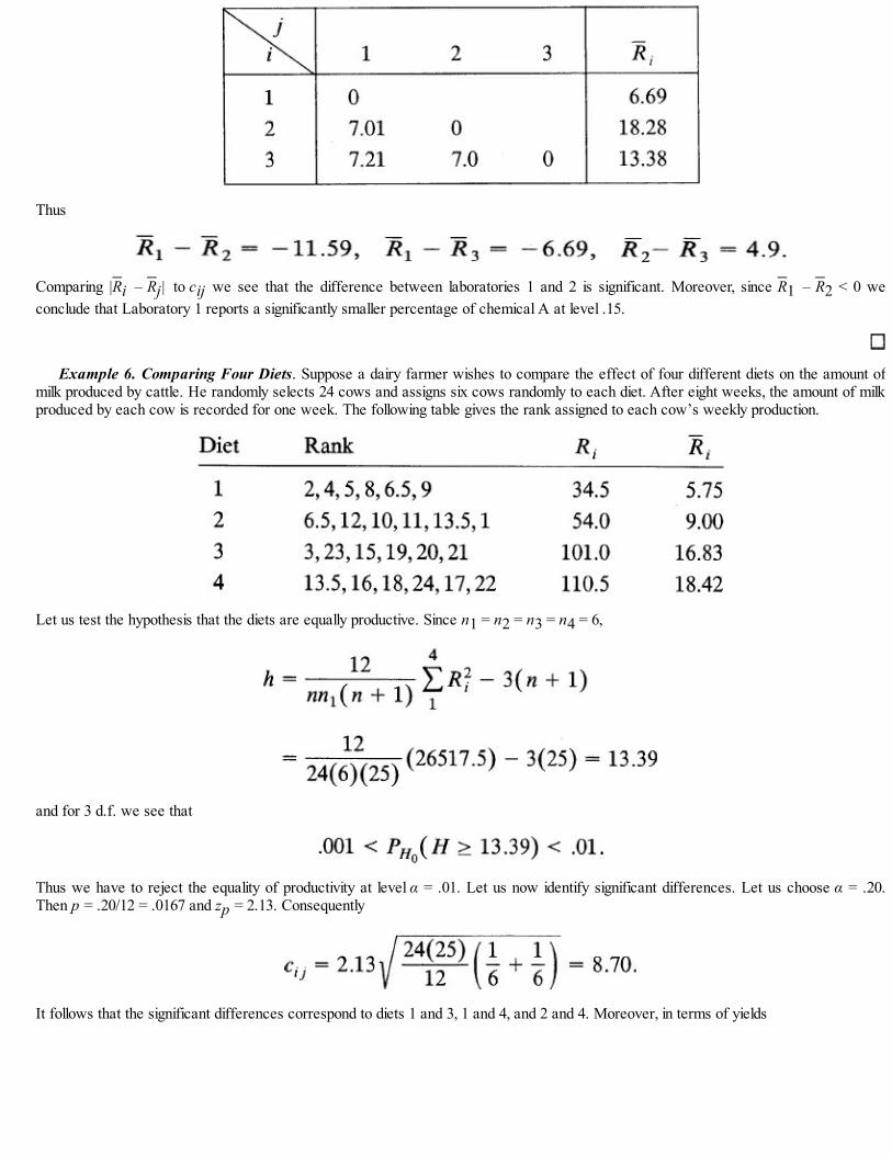
Thus

Comparing |Ri – Rj| to cij we see that the difference between laboratories 1 and 2 is significant. Moreover, since R1 – R2 < 0 weconclude that Laboratory 1 reports a significantly smaller percentage of chemical A at level .15.

Example 6. Comparing Four Diets. Suppose a dairy farmer wishes to compare the effect of four different diets on the amount ofmilk produced by cattle. He randomly selects 24 cows and assigns six cows randomly to each diet. After eight weeks, the amount of milkproduced by each cow is recorded for one week. The following table gives the rank assigned to each cow’s weekly production.

Let us test the hypothesis that the diets are equally productive. Since n1 = n2 = n3 = n4 = 6,

and for 3 d.f. we see that

Thus we have to reject the equality of productivity at level α = .01. Let us now identify significant differences. Let us choose α = .20.Then p = .20/12 = .0167 and zp = 2.13. Consequently

It follows that the significant differences correspond to diets 1 and 3, 1 and 4, and 2 and 4. Moreover, in terms of yields

so with 80 percent confidence we can state that diet 4 is more productive than diets 1 and 2 and that diet 3 is more productive than diet 1.

Problems for Section 13.5

1. The United Way would like to compare contributions to its annual appeal in three different towns.Independent random samples of contributors are selected from contribution records for each town andthe annual contributions for each contributor in the sample are recorded.

Town Annual Contributions(dollars)1 35, 150, 200, 45, 75, 52 15, 110, 75, 25, 30, 115, 1253 25, 35, 30, 75, 225, 160

Is there sufficient evidence to conclude that the average (median) contribution in each town is thesame? Analyze the data by using the large sample median test (even though n = 19) as well as theKruskal–Wallis test.

2. In order to compare the amount of time it takes to recover from four different types of influenza, arandom sample of 32 volunteers was selected. Eight subjects each were randomly assigned to eachstrain of virus. Each subject was then injected with the strain of the virus and all 32 subjects thenreceived the same care. The number of days it took for each subject to recover completely wasrecorded as follows:

InfluenzaType Recovery Time (Days)

1 5, 7, 5, 8, 12, 6, 4, 52 4, 7, 3, 4, 6, 6, 5, 43 8, 12, 13, 10, 11, 10, 9, 114 12, 10, 13, 12, 14, 10, 13, 12

(i) Is there sufficient evidence to indicate that the recovery times for the four types of influenza arethe same? Apply the median test and the Kruskal–Wallis test and compare your results.

(ii) If the recovery times are significantly different, identify the differences at level α = .15.

3. In a study to compare the mean weight at four different heights, random samples of males from eachheight group are selected and their weights are recorded as follows:

Height Group (cm) Weight (kg)[150, 160) 50, 54, 52, 55, 52, 51

[160, 170) 55, 60, 62, 64, 61, 60[170, 180) 65, 68, 67, 66, 67[180, 190) 72, 75, 80, 79, 82, 81, 74

(i) Is the distribution of weight the same for the four height groups? Compare the Kruskal–Wallistest and the one-way analysis of variance F-test.

(ii) Identify significant differences if any at level α = .25.

4. In order to check if there are significant differences in reading ability across the state, the State Boardof Education classifies each school district as urban, suburban, or rural. From each district medianreading scores of high school seniors are then recorded as follows:

Distric Median ScoreUrban 15.2, 14.7, 15.6, 14.8, 16.2, 13.4, 16.1Suburban 17.8, 19.4, 16.8, 18.3, 20.3, 18.6, 19.8, 20.7Rural 12.6, 14.3, 11.2, 13.4, 14.5, 15.1

Is there sufficient evidence to indicate that the median scores differ among the three classifications? Ifso, identify significant differences at level α = .25.

5. Six different automobile models advertise the same fuel efficiency as measured by miles per gallon ofgasoline. Randomly selected cars of each model were run on five gallons of the same brand ofgasoline until the gas runs out. The road and weather conditions for each test run were identical. Thefollowing table gives the number of miles traveled by each car.

Model Miles TraveledA 66, 68, 67, 70, 69, 68, 71, 72B 71, 75, 78, 79, 76, 78, 76C 89, 90, 95, 90, 92, 96, 94D 107, 105, 98, 106, 104, 95E 115, 118, 122, 116, 118, 117F 130, 132, 121, 129, 130, 126

Test the hypothesis that the distributions of the number of miles traveled are the same for each model.Identify significant differences if any at level α = .20.

6. The following table gives the hourly wages of samples of floor workers in four different departmentstores in Toledo.

Department Store Hourly WageA 3.35, 3.80, 3.55, 3.35, 3.80B 3.80, 4.10, 4.10, 3.95, 4.25, 4.40C 4.00, 4.50, 4.50, 4.70, 5.00D 3.35, 3.80, 4.10, 3.95, 3.80

Test the hypothesis that the distributions of the hourly wages are the same for the four stores.Investigate significant differences if any at level α = .15.

7. Show that the Kruskal–Wallis statistic and the Mann–Whitney–Wilcoxon test statistic offer equivalentcriteria in the k = 2 case when n is large and each ni is large. That is, show that (4) and (6) areequivalent when k = 2.

8. Show that expressions (6) and (7) for H are equivalent.

13.6 THE FRIEDMAN TEST FOR k-RELATED SAMPLES

In Section 13.5 we studied two methods of testing the equality of k distribution functions based on k-independent random samples. The Kruskal–Wallis test that we studied as an extension of the Mann–Whitney–Wilcoxon test is an analog, as we saw, of the one-way analysis of variance when we replace thenormality assumption by the assumption that the distribution functions are all continuous. We nowconsider a statistic used in the analysis of data resulting from k-related samples. The problem weconsider now may be regarded as an extension of the problem of dependent (or matched) pairs ofobservations considered in Section 11.5. The Friedman test statistic that is used to analyze k-relatedsamples is, however, not an extension of the Wilcoxon signed rank test of Section 11.5. Indeed, it does notrequire the assumption of symmetry needed for the Wilcoxon test. The Friedman test is an extension of thetwo-way analysis of variance technique for a randomized block design when the assumption of normalityis replaced by the assumption that the distributions are continuous.

Let (Xi1, Xi2, …, Xik), i = 1, 2, …, b be a random sample from a k-variate continuous type distributionfunction. The observations may be arranged in b rows (called blocks) and k columns (called treatments).The observations in different rows are independent and those in different columns are dependent. Theobservation xij then corresponds to the ith block and jth treatment, i = 1, 2, …, b and j = 1, 2, …, k. Theobject is to test the null hypothesis H0: treatment effects are all equal, against the alternative hypothesisH1: treatment effects are not all equal.

Friedman suggested replacing each observation in a block by its rank. In the Kruskal–Wallis test wereplace each observation by its rank in the combined sample in order to compare every observation withevery other observation. In the present setup it does not make much sense to compare observations in twodifferent blocks. Hence ranks are assigned separately for each block. We assume for now that there are notied observations within each block.

Let Rij = R(Xij) = rank of jth observation in ith block. Then 1 ≤ Rij ≤ k. Let

Clearly

whereas the Rj’s are random. If the treatment effects are all the same then we expect each Rj to be equal tob(k + 1)/2. That is, under H0,

The sum of squares of deviations of Rj’s from H0Rj therefore is a measure of the differences in treatment

effects. Let

The Friedman test statistic is defined by

We leave the reader to show (Problem 8) that (1) may be rewritten in the form

which is more convenient for computational purposes.The null distribution of F is extensively tabulated for small values of k and n. The null distribution of

F can be approximated by a χ2(k – 1) distribution. The approximation gets better as b gets larger. In orderto avoid giving long tables we will use this approximation. The null hypothesis is rejected at level α if thecomputed value of F exceeds χ2

k – 1, α, the quantile of order 1 – α for a χ2(k – 1) random variable.

Friedman Statistic for Testing Equality of k Treatment Effects

Let Rij = rank of Xij, 1 ≤ Rij ≤ k , and = sum of ranks for jth treatment. Compute

Reject H0: no treatment differences at level α if the computed value f of F satisfies

Theoretically, ties within each block occur with probability zero. In practice, however, ties do occur.Tied observations are assigned average rank and the value of F is computed in the usual way.

Example 1. Weight Gains by Swines (Example 13.4.4). In Example 13.4.4 the weight gains (in pounds) by swines fed on threerations were as follows.

We saw that we cannot reject H0: no difference in rations at α = .05 level. In order to apply the Friedman test we rank the rations ineach block from 1 (least weight gain) to 3 (most gain) as follows.

Since b = 5, k = 3, we have

so that for k – 1 = 2 d.f. the approximate P-value satisfies .20 < P-value = P(χ2(2) ≥ 2.8) < .30. Thus we cannot reject H0. (The exact P-value in this case, is, in fact, .367.)

Example 2. Comparing Tire Durability of Four Brands . Four brands of automobile tires are to be tested for durability. Threedrivers are selected for the experiment. Each driver is given a set of four tires. The tires are mounted in a random fashion on his car androtated regularly. The car is run for 10,000 miles and the tread wear is measured. The experiment is then repeated with a second set offour tires of a different brand, and so on. Ranks are assigned by each driver to the four brands of tires according to the tread wear (rank 1is assigned to the brand with the most tread wear, etc.). The following table shows the ranks and rank sums.

Do the data indicate a significant difference in durability as measured by tread wear?

Here b = 3 and k = 4, so that

For k – 1 = 3 d.f. we see that

so that we reject H0 at α = .10 but not at α = .05. Thus at significance level .10 we conclude that there are significant differences in tiredurability.

Remark 1. Suppose k = 2 so that two treatments are to be compared. In this case the randomized blockdesign reduces to the paired comparisons design. The appropriate test for paired comparisons is the signtest of Section 6.3. How does Friedman test compare with the sign test in this special case? We note thateach block has two ranks, 1 and 2. Suppose X = number of blocks in which treatment 1 receives rank 1and treatment 2 rank 2. Then

and

The null hypothesis is rejected when F is large, or equivalently, when |X/b – 1/2| is large. Since X is thenumber of pairs for which the second treatment is “better” than the first we see that the F test is equivalentto the two-sided sign test based on the differences Xi1 – Xi2, i = 1, 2, …, b, provided b is large.

Remark 2. Suppose b = 2 so that there are only two blocks.

In Section 11.9.1 we used the Spearman rank correlation coefficient Rs given by

as a measure of disagreement between the two sets of rankings. What, if any, is the relation between F andRS? We leave the reader to show (Problem 9) that

so that the Friedman test may also be used as a test of linear dependence in the two-sample case.

Remark 3. The Problem of b-Rankings. A statistic designed as a measure of agreement between bsets of rankings is closely related to the Friedman test statistic F. This is the so-called Kendall’scoefficient of concordance defined by

One can show (Problem 10) that 0 ≤ W ≤ 1. If all the b sets of rankings are in complete agreement, thenR1, R2, …, Rk is a permutation of b, 2b, …, kb and it follows that W = 1. Thus values of W near 1 may beinterpreted to mean that there is perfect agreement (or perfect association) among rankings. Similarly,values of W near zero may be interpreted to mean no agreement (or no association) among rankings. Thestatistic W may be used to test the null hypothesis of no association or independence among b rankingsagainst the alternative that some association exists. (See Section 11.9 for the bivariate case.)

Example 3. Wine Testing . Six judges were asked to rank eight different brands of nonvintage Rosé wines all of which sell forapproximately the same price. The following table shows their rankings. (Rank 1 means most preferred, rank 8 least preferred.)

Suppose first that we are only interested in measuring the association among the six sets of rankings. We compute

so that there is strong agreement among the rankings.Let us test H0: no association against H1: association exists. We see that

and for k – 1 = 8 – 1 = 7 d.f. we have

Thus we reject H0 and conclude that the judges agree reasonably well in their rankings of the wines.If the (column) rank sums are used to estimate the ordering of judges’ preferences then the preference ordering (from most preferred

to least preferred) is as follows:

Thus the estimate of the rank of Brand A is 1, of Brand B is 3, of Brand C is 2, and so on.

Remark 4. In the beginning of this section we said that Friedman’s test is an extension of the two-wayanalysis of variance technique carried out by replacing each observation in a block by its rank in theblock. We leave the reader to show (Problem 11) that

so that from (1)

Let Rj = Rj/b and . Then we can partition TSS as

The block sum of squares, SSB, is zero since the block sums are equal to k(k + 1)/2, so that there is novariation among the blocks. Thus the F-statistic in the two-way analysis of variance for testing H0: nodifferences in treatments is the ratio

where from (1)

Since TSS is a constant, the Friedman statistic is analogous to the F-ratio in the two-way analysis ofvariance.

Multiple Comparisons

When the Friedman test rejects the null hypothesis that the treatment effects are all the same, it is ofinterest to identify significantly different treatments. The procedure for multiple comparison is similar tothe one outlined in Section 13.5.3. Indeed

where zp is the quantile of order 1 – p under the standard normal distribution and p = α/k(k – 1). Thusthose pairs of treatment sums (Ri, Rj) are significantly different at level α for which

The sign of Ri – Rj determines the direction of the difference.

Example 4. Multiple Comparisons in Example 2. In Example 2 we concluded that there were significant differences in tiredurability at level .10. The data suggest that Brand C and D tires are more durable than Brand A and B tires. Let us apply the method ofmultiple comparisons to see if this is in fact the case. Let us choose α = .15 so that p = .15/4(3) = .0125 and z.0125 = 2.24. Thus

Since none of the |Ri – Rj|, i ≠ j, equals or exceeds 7.08 we cannot conclude at an overall level .15 that any pairs of treatments aresignificantly different.

If, on the other hand, we compare only Brands A and C, then with k = 2, α = .05, p = .05/2 = .025, and zp = 1.96 we have

Since |RA – RC| = |R1 – R3| = 6.5 > 3.39 we conclude that Brand A and Brand C tires are significantly different at level .05. Moreover,since R1 < R3 we conclude that Brand C tires are more durable (that is, have less tread wear) than Brand A tires.

Example 5. Comparing Five Gasoline Additives . In an experiment to compare five gasoline additives three different car modelsare used. Each car is driven five times on the same course for 200 miles, once with each additive. All cars use the same gasoline. Thefollowing table gives the ranks assigned to gasoline mileage per gallon of gasoline for each car. (Rank 1 means lowest mpg.)

We note that k = 5, b = 3 and

For k – 1 = 4 d.f. we see that

and we reject H0: no differences in additives at level α = .05.Let us now perform multiple comparisons to identify any significant differences. Choosing α = .20 we see that zp = z.01 = 2.33 and

Writing i = 1, 2, 3, 4, 5 respectively for A, B, C, D, and E we see that

so that of all the pairs the only pair that differs significantly at level .20 is the pair (D, E). Moreover, since R5 > R4 we conclude that theadditive E is more effective in increasing gasoline mileage than additive D.

Problems for Section 13.6

1. In the randomized block experiment of Problem 13.4.5 the yield (pounds per plot) of four varieties of wheat obtained with three fertilizerswere as follows.

Using the Friedman test, test the hypothesis that the yield produced by the four varieties of wheat are not significantly different. Compareyour result with the parametric case of Problem 13.4.5.

2. In a study of six groups under five different conditions, each group is assigned five matched subjects, one assigned to each of the fiveconditions. The following table gives the scores.

Using Friedman’s statistic, test the hypothesis that all the samples come from the same population.

3. In an experiment to study the effectiveness of five over-the-counter sleeping aids, eight subjects were selected. The experiment was

conducted over a period of five weeks. Each subject received one of the five brands of sleeping aids for a week and was given a differentbrand for each subsequent week. The average number of hours of sleep was recorded as follows.

Test the null hypothesis that the five brands of sleeping aid medicines are equally effective.

4. In an experiment a psychologist asked 10 subjects to recall some material after five different time intervals. The degree of recall was thenranked for each subject from 1 to 5 (1 for least recall and 5 for most) with the following results.

Could the difference among rank sums be attributed to chance variation?

5. Suppose 10 randomly selected students are ranked in five subjects, English, Mathematics, History, Geography, and Economics from 1(worst) to 10 (best) with the following results.

Test the hypothesis of no agreement in the five sets of rankings. Estimate, if possible, the relative rank of each student in the five subjects.

6. In a dance contest, five judges are asked to rank each of the 10 finalists from 1 (best dancer) to 10 (worst dancer) with the followingresults.

(i) Compute Kendall’s coefficient of concordance.(ii) Test the hypothesis that there is no association among the rankings.(iii) If the null hypothesis of no association in part (ii) is rejected, estimate the rank of each contestant.

7. The following are the scores obtained by a group of fifth graders on tests in arithmetic, social studies, reading, and language.

(i) Compute Kendall’s coefficient of concordance.(ii) Test the hypothesis that there is no agreement among the four sets of rankings of a student’s performance.(iii) If the null hypothesis in (ii) is rejected, estimate the relative ranks of the eight students.

8. Show that F can be written in the form

9. Show that in the b = 2 case the Friedman statistic and the Spearman’s rank correlation coefficient are related according to the relation

10. Show that W, the Kendall coefficient of concordance, satisfies the inequality 0 ≤ W ≤ 1. [Hint: W takes the least value when all the ranksums are equal to their mean value.]

11. Show that

(i) ,

(ii)

13.7 REVIEW PROBLEMS

1. In a study to determine whether there is a significant difference among the I.Q. scores of children of poor, lower middle class, middleclass, upper middle class, and affluent families the following results are obtained based on independent random samples:

Economic Status I.Q. Scores

Poor 122, 115, 106, 112, 98, 105Lower middle 120, 114, 97, 104, 112Middle 115, 110, 100, 118, 98Upper middle 124, 102, 99, 108, 118, 131Affluent 104, 108, 110, 101, 115, 124, 116, 128

Is the difference among the sample mean I.Q. scores significant at the 1 percent level? Perform a one-way analysis of variance.

2. The following data give the service times (in minutes) that four tellers at a local bank spent serving their customers. The customers servedby each teller were selected at random.

Teller Service Times (minutes)1 3.8, 1.7, 0.6, 2.3, 1.1, 1.42 4.5, 5.0, 3.8, 2.7, 4.23 3.2, 3.5, 4.0, 2.8, 4.64 1.6, 2.0, 2.8, 0.6, 1.2, 1.8, 1.2

(i) Is the difference among the sample mean service times of the four tellers significant at level .05? Perform a one-way analysis ofvariance.

(ii) If the answer to part (i) is yes, identify the significantly different true means at level .05.

3. In order to compare the effects of four stimuli on the reaction time of adult males, a completely randomized design was used. Twentysubjects were randomly assigned the four stimuli. The following reaction times (in seconds) were recorded.

Stimulus Reaction TimesA 1.1, 1.4, 1.2, 1.3B .3, .4, .2, .4, .3C .8, .6, .7, .9, .8, .7D .6, .4, .5, .7, .3

(i) Test the null hypothesis that the mean reaction times to the four stimuli are equal. Construct simultaneous confidence intervals for allthe six differences among the mean reaction times at overall level at least .95. Identify significantly different means.

(ii) Since the reaction time varies from individual to individual, the experimenter decides to redesign the experiment with subjects asblocks. Five subjects are used in this newly designed experiment. Each subject is randomly assigned to each of the four stimuli. Thefollowing table shows the reaction times of the twenty subjects.

Construct the two-way analysis of variance table and test the null hypothesis that the mean reaction times to the four stimuli are allequal. Find simultaneous confidence intervals for the pairs of differences among the stimuli means at overall level .95.

(iii) In part (ii) apply Friedman’s test to test the null hypothesis of no difference among the four stimulii.

4. Six brands of cigarettes are to be compared for tar content. Independent random samples of cigarettes of each brand are tested to yieldthe following tar levels (in milligrams).

Brand Tar Content (mg)A 4.2, 4.6, 4.4, 4.8, 4.4B 6.4, 6.8, 6.2, 6.5, 7.0C 8.1, 5.9, 7.3, 7.8, 6.6, 8.4D 5.0, 5.4, 5.3, 5.2, 5.2

E 7.2, 6.9, 7.6, 7.4, 7.1F 3.2, 3.1, 3.8, 3.6, 3.4

(i) Test the null hypothesis that the mean tar levels of each brand of cigarette are the same at level .05 using a one-way analysis ofvariance.

(ii) Do the same using a Kruskal–Wallis test.

5. Fifty female applicants for the positions of school bus drivers are given a psychological test in order to test their ability to stay calm andhave self-control under trying conditions. The following table gives the scores of 50 applicants, classified according to their age group.

(i) Are there significant differences among the age groups of applicants in the ability to stay calm and in control? Use one-way analysisof variance. If so, identify significantly different age groups at level α = .05.

(ii) Apply the Kruskal–Wallis test to the same data to test the hypothesis that distribution of scores is the same for each age group.Identify significantly different age groups at level α = .15.

(iii) State the difference in assumption in the two methods of analysis and compare your results.

6. The Internal Revenue Service wishes to compare the average time it takes to complete four different versions of the short form that it hasdeveloped. Twenty-five taxpayers who file the short form are selected and each is randomly assigned to one of the four forms. Theamount of time it takes to complete the form (in minutes) is recorded as follows.

Test the hypothesis that the four versions of the short form require the same average time to complete and identify significantly differentmeans if any:

(i) Use the one-way analysis of variance.(ii) Use the Kruskal–Wallis test.

7. The following data give the grade-point averages of 30 students by sex and major academic field of study.

Perform a two-way analysis of variance and test the null hypothesis of no sex effect, no field of study effect, and no interaction effect ongrade-point averages.

8. Three doses of an antidiuretic substance are administered to rats. Three rats are taken from each of four litters, and one of the three dosesis given to each rat randomly. Each experimental rat is given a standard water load at the beginning of the experiment. The following tableshows the amount of urine collected in the next 60 minutes as a percentage of the standard load.

(i) Are the differences among the doses significant at the 5 percent level?(ii) Are the differences among the litters significant at the 5 percent level?(iii) Find simultaneous confidence intervals for the differences in doses at an overall level of at least .95.(iv) Use the Friedman test to test the null hypothesis of no dose effect.

9. In a consumer survey, seven consumers are asked to rank in order of preference four methods of packaging an over-the-counter painreliever. The object of the study is to determine if there are differences among the four methods of packaging and if so, to estimate therelative order of preference of the four methods. The following table gives the ranks assigned (1 for the most preferred and 4 for the leastpreferred).

Analyze the data to carry out the objectives of the study.

10. Fifteen students were grouped according to their grades on a pretest in mathematics. Three sections of a new course were set up. Thesame teacher taught the three sections using the same method and the same material. The following table gives the average grade foreach student in this new course.

Rank the students in each of the five groups according to their grade (1 for lowest, 3 for highest). Compute Kendall’s coefficient ofconcordance and test the null hypothesis of no association.

11. In a flower show the judges agreed that five exhibits were outstanding. These exhibits were numbered arbitrarily from 1 through 5 andpresented to four judges for ranking in order of merit. The following rankings were obtained.

Compute Kendall’s coefficient of concordance and test the null hypothesis of no association among the four rankings.

† See, for example, W. J. Conover, Practical Nonparametric Statistics, Wiley, 1971, p. 393.‡ See J. D. Gibbons, Nonparametric Methods for Quantitative Analysis, Holt, Rinehart and Winston, 1976, pp. 178–179.

Appendix—Tables

TABLE Al. Random Digitsa

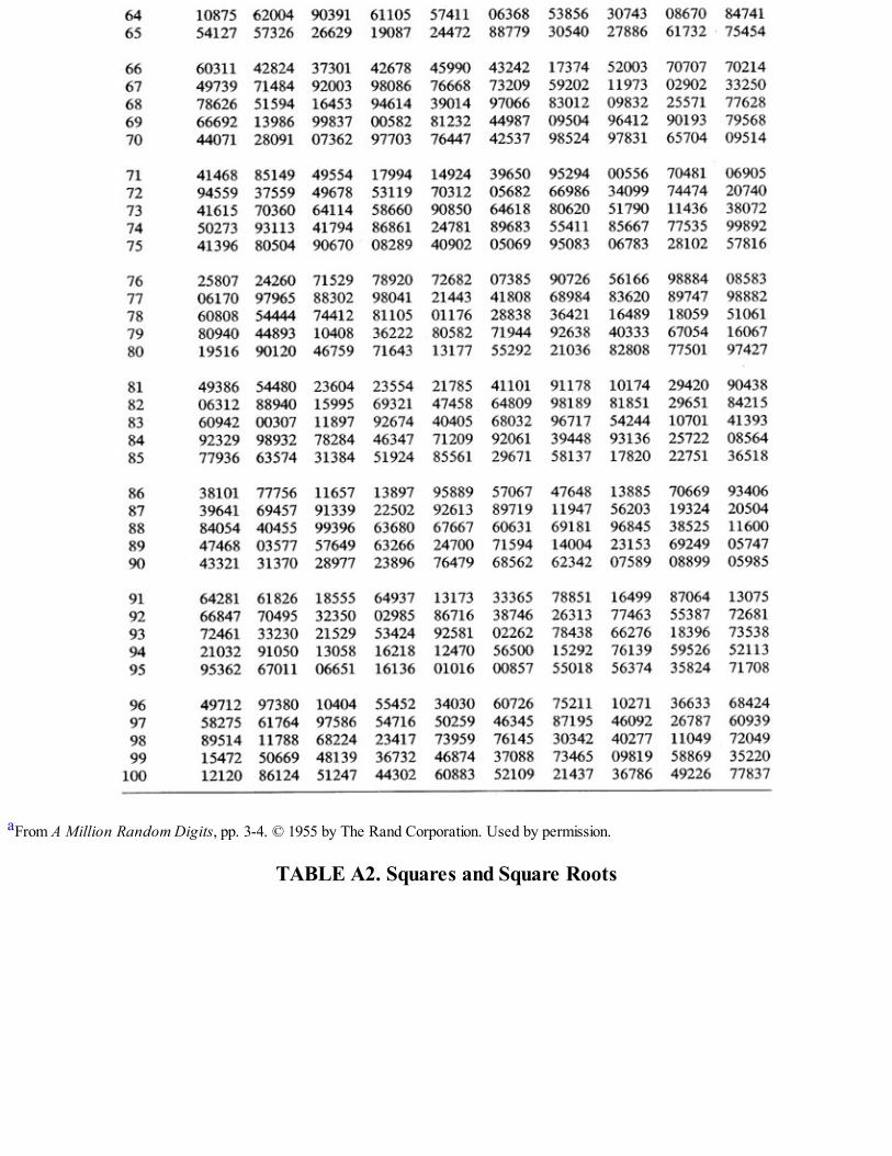
aFrom A Million Random Digits, pp. 3-4. © 1955 by The Rand Corporation. Used by permission.

TABLE A2. Squares and Square Roots

TABLE A3. Cumulative Binomial Probabilitiesa

aFor n = 2 to 20 and n = 25, from Tables of Cumulative Binomial Probability Distribution , Harvard University Press, Cambridge,Massachusetts, 1955, reprinted with permission. For n = 100, from 50–100 Binomial Tables by H. G. Romig, copyright 1947, Bell TelephoneLaboratories, Short Hills, .J., reprinted with permission.

TABLE A4. Cumulative Poisson Probabilitiesa

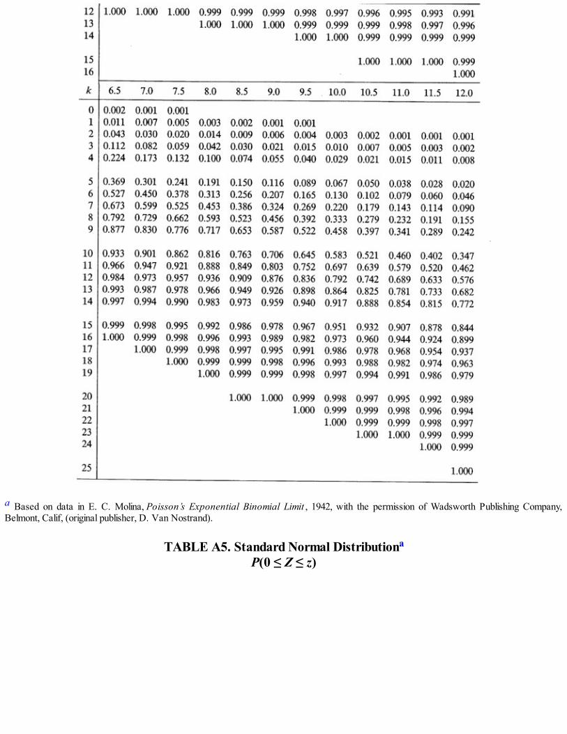
a Based on data in E. C. Molina, Poisson’s Exponential Binomial Limit , 1942, with the permission of Wadsworth Publishing Company,Belmont, Calif, (original publisher, D. Van Nostrand).

TABLE A5. Standard Normal Distributiona

P(0 ≤ Z ≤ z)

aReprinted from A. Hald, Statistical Tables and Formulas, Wiley, New York, 1953, with permission.

TABLE A6. Distribution of ta

aReprinted from Table III of Ronald A. Fisher and Frank Yates, Statistical Tables for Biological, Agricultural, and Medical Research, 6thed., Longmans Group Ltd., London (previously published by Oliver and Boyd Ltd., Edinburgh), 1974, by permission of the authors andpublishers.

TABLE A7. Distribution of Χ2a

aReprinted (except for α = .975 and .025) from Table IV of Ronald A. Fisher and Frank Yates, Statistical Tables for Biological,Agricultural, and Medical Research, Longmans Group Ltd., London (previously published by Oliver and Boyd Ltd., Edinburgh), bypermission of the authors and publishers.bValues for α = .975 and .025 are taken from Table 3 of E. S. Pearson and H. O. Hartley, Biometrika Tables for Statisticians, Vol. II, 1972with permission of the Biometrika Trustees.cFor larger values of n, the expression may be used as a normal deviate with unit variance, remembering that the

probability for χ2 corresponds with that of a single tail of the normal curve.

TABLE A8. F-Distribution: 5 Percent (Roman Type and)

1 Percent (Boldface Type) Points for the Distribution of Fa

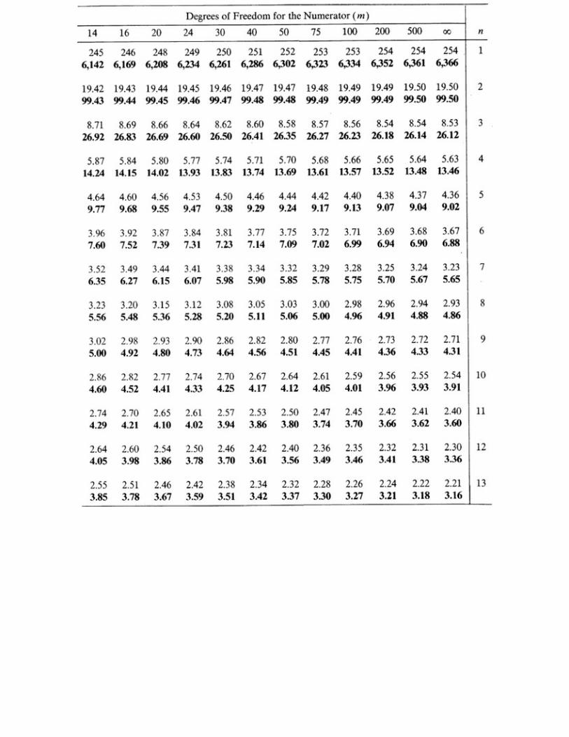
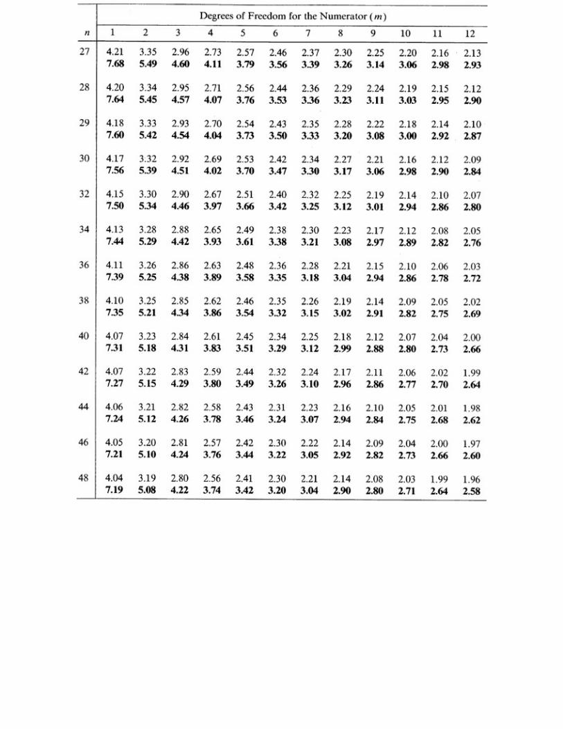
aReprinted by permission from George W. Snedecor and William G. Cochran, Statistical Methods, 7th Ed., © 1980 by the Iowa StateUniversity Press, Ames, Iowa 50010.

TABLE A9. Right Tail Probabilities for One-Sample Kolmogorov-Smirnov Statistica

aAdapted from L. H. Miller, “Tables of Percentage Points of Kolmogorov Statistic,” Journal of the American Statistical Association, 51(1956), 111-121, with the permission of the American Statistical Association.

Table A10. Right Tail Probabilities P(Tx ≤ tx) for Mann-Whitney-Wilcoxon Text Statistica

Right tail probabilites are given for tx ≤ m(m + n + 1)/2 for m ≥ n. Left tail probabilities are obtainedfrom the relation

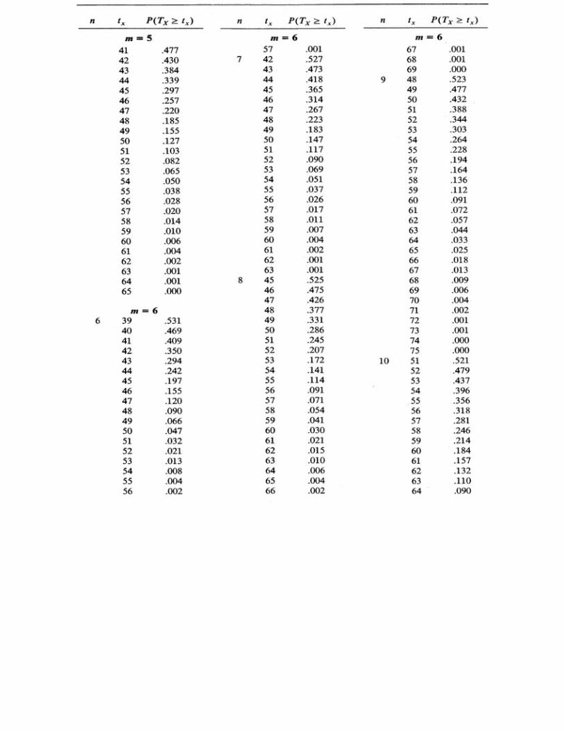
aReprinted with permission of Macmillan Publishing Company from Charles H. Kraft and Constance Van Eeden, A NonparametricIntroduction to Statistics, Copyright © 1968 by Macmillan Publishing Company.

TABLE A11. Cumulative Right Tail Probabilities For Wilcoxon Signed Rank Statistica

Right tail probabilities P(W ≥ W0) are given for w0 ≥ n(n + l)/4. Here W is interpreted as either W+ or W–. Left tail probabilities are obtained from the relation P(W_ ≤ n(n + l)/2 – w0).

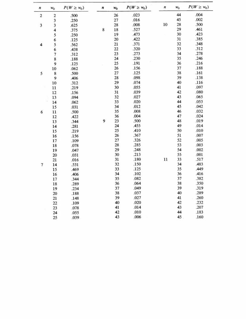
aFrom Table II of H. L. Harter and D. B. Owen, Eds, Selected Tables in Mathematical Statistics, Vol. 1, Markham, Chicago, 1972, with thepermission of the Institute of Mathematical Statistics.

Table A12. Left Tail Cumulative Probabilities, P(R ≤ r), for Total Number of Runs R.a

aReprinted from Frieda S. Swed and C. Eisenhart, “Tables for Testing Randomness of Grouping in a Sequence of Alternatives,” Annals ofMathematical Statistics, 14 (1943) 66–87, with the permission of the Institute of Mathematical Statistics.

Table A13. Cumulative Probabilities P(R ≥ r) for Spearman’s Rank Correlation Statistic Rs = r.a

Right tail probabilities are given for r ≥ 0. Left tail probabilities may be obtained from symmetry: For r >0, P(R ≥ r) = P(–1 ≤ R ≤ –1).

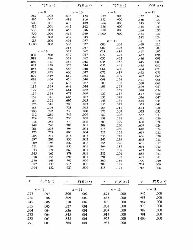
aFor 4 ≤ n ≤ 11, adapted from Table 13.2 of Donald B. Owen, Handbook of Statistical Tables, © 1962, U.S. Department of Energy,published by Addison-Wesley Publishing Company, Inc., Reading, Massachusetts; reprinted with permission of the publisher.

For 12 ≤ n ≤ 30, adapted from G. J. Glasser and R. F. Wintner, “Critical Values of the Rank Correlation Coefficient for Testing theHypothesis of Independence,” Biometrika, 48 (1961), 444–448, with permission of the Biometrika Trustees.

TABLE A14. Cumulative Probabilities for Kendall’s Tau Statistica

Left tail probabilities may be obtained from symmetry: For

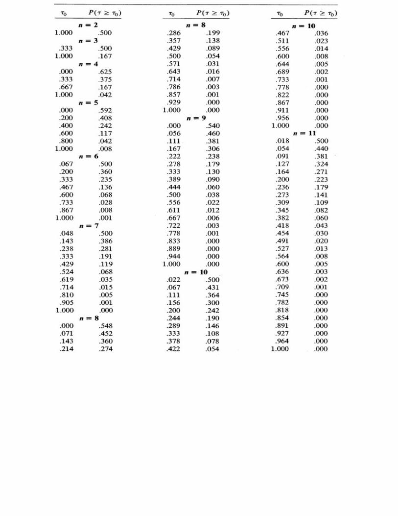
aFor 2 ≤ n ≤ 12, adapted from Table 13.1 of Donald B. Owen, Handbook of Statistical Tables , © 1962, U.S. Department of Energy,published by Addison-Wesley Publishing Company, Inc., Reading, Massachusetts; reprinted with permission of the publisher.

For 14 ≤ n ≤ 30, adapted from L. Kaarsemaker and A. van Wijngaarden, “Tables for Use in Rank Correlation,” Statistica Neerlandica, 7(1953), 41–44, with permission.

Answers To Odd-Numbered Problems

SECTION 2.2

1. (i) {(i, j, k): i, j, k {H, T}}; (iii) Each point of Ω is a subset of 13 cards from {AC, 2C,…,KC,…,AS, 2S,…,KS}; (v) {0, 1,…,n}; (vii) {2, 3, 4, 5, 6}; (ix) {(x, y, z): x ≥ 1 integral, y > 0, z > 0} (xi){(x, y): 0 ≤ y ≤ x ≤ 1}; (xiii) {(i, j, k, l, m): i, j, k, l, m {L, R}}.

3. (i) (a) (c) (C – A) ∪ (A – C).5. {(X, y, Z), (X, Z, Y), (Y, X, Z), (Y, Z, X), (Z, X, Y), (Z, Y, X)}; {(X, Y, Z), (X, Z, Y),(Z, X, Y)}; {(X, Y,

Z),(X, Z, Y)}; {(Y, X, Z), (Z, X, Y)}.7. (i) {(x, y): 0 ≤ x ≤ y ≤ 1}; (iii) {(x, y): 0 ≤ y ≤ 3x, 0 ≤ x ≤ 1, 0 ≤ y ≤ 1}.9. All subsets of three cities; (i) {{D, P, L}, {D, P, H}, {P, L, H}, {D, L, H}}, etc.

SECTION 2.3

1. In parts (ii), (v) and (vii).3. 24/30; 28/30; 28/30.5. 2/10; 7/10; 4/10.7. 6/8.9. 1/9.

11. 4/9; 5/9.

SECTION 2.4

1. 1/5; 4/5; 12/25; 1/10; 4/125.3. .94; .18, .05; .95; .93, .82.5. .0106.7. 0.9. ≥ .45.

11. .75; .2; .05.13. .05; .04; .15; .15; .16; .84; .40; .38; .60.15. .75 ≤ p ≤ .8; .1 ≤ p ≤ .55; .2 ≤ p ≤ .25.

SECTION 2.5

1. 1680.3. 109 (or 9(10)8 if number cannot begin with zero).5. 4!; 44.7. ll!/(2!)3.9. 45321.

11. 7; 6.

13. .

15. .

17. 20!/5! 12! 3!.19. 3/103(26)3.21. Yes, P(all men) = 6/143.23. 1/22.25. 1/3; 2/5.27. (1 – 2/(N – 1))2n–2.29. .

31. Yes, probability .0151.33. 1 – 999990P3/1000000P3 = .00003.

SECTION 2.6

1. 26/48; 32/52; 20/52; 22/48.3. 100/126.5. 8/13; .02.7. .08.9. 36/91.

11. 1/4; 1/3.13. .08.15. 173/480; 108/173, 15/173.17. .0872.

SECTION 2.7

1. (vi).3. Yes.5. 0 or 5/7; .5.9. .5 or .2; .2 or .5.

11. 1 – (1 – e–t0/λ.13. .001; .1; .05; .352; .216.15. 1 – (.95)20 – (.95)19.19. (i) 16807/279936; (ii) .463, .386, .1285, .0214, .0018, .0001 for j = 1, 2,…, 6, etc.21. plp2(2 – p1)(2 – p2).

SECTION 2.8

5. 10p5/105.7. 9; 9.

SECTION 2.9

1. Yes in each case.5. (n – r + 1)!/n!.9. (1 – p)/(2 – p); 1/(2 – p).

11. 1/6; 1/3; 1/3.

13. π/(π + p(1 – π)).15. 1/18; 1/17.17. .90 ≤ P(∪Ai) ≤ .95.19. 13/16; 4/13; 12/13.21. .00000064; .00043.23. 1 – π/4; σ/4; σ/4; 0.

SECTION 3.2

3. 1/2, 1/2; 1/29.7. 16/210, 8/210, 48/210, 48/210.9. (ii) 16/27, 49/81, 5/9.

SECTION 3.3

1. No; yes; yes; no.3. P(X = 0) = .18, P(X = 1) = .54, P(X = 2) = .27, P(X = 3) = .02; .82.5. c = 2/15; 1/49; 2/N(N + 1); P(X < 3) = 13/15, 9/49 6/N(N + 1); smallest x = 1, 4,

; largest x = 0, 3, .7. .8647, .4059, .2706.9. 1 — exp{ — (x — θ)/λ} for x ≤ θ; 1/2 + (arctan x)/σ.

11. Yes; 1/2 for 0 < x < 1, 1/4 for 2 < x < 4; 1/2θ, |x| ≥ θ; xe–x, x < 0; (x – l)/4 for 1 ≤ x < 3, and P(X =3) = 1/2; 2xe–x2, x > 0.

13. .3679; .141; .6988.15. .2.17. 20e–5, 3/16.19. [e–2/λ + (1 – p)2]/3; 0, e–2/λ[e–2/λ + (1 – p)2]–1, (1 – p)2[e–2/λ + (1 – p)2]–1.

SECTION 3.4

1. (ii) 11/36, 13/36.3. (ii) 5/16, 3/8.5. (ii) 23/60, 7/10, 23/60.9. , for |x| ≤ 1, |y| ≤ 1.

11. Yes, 1 – e–7.13. (iii) 3/4, 9/16.15. 1/24; 15/16.17. f(x, y) = 1, 0 ≤ x ≤ y ≤ ; 1/4, 19. 1/6, 2/3.

SECTION 3.5

1. (ii) X: 64/216, 48/108, 12/54, 1/27; Y:27/216, 27/72, 9/24, 1/8; (iii) P{X = x|Y = y} =

(3/4)y(1/4)3 – x – y, P{Y = y|X = x} = (2/3)x(1/3)3 – y – x; (iv) 24/47.

3. X: 9/54, 8/48, 7/42, 6/36, 5/30, 4/24; Y: 1/54, 17/432, 191/3024, 257/3024, 1879/15120,2509/15120, 2509/15120, 2509/15120, 2509/15120.

5. (i) ; (ii) , ;

(iv) 1/84, 4/84; (v) 1/5, 1/10.7. (i) 3x/4 + 5/8; 3/8 + 5y/4; (ii) 105/128, 81/128; (iii) h(y|x) = 2(3x + 5y)/(6x + 5), g(x|y) = 2(3x +

5y)/(3 + 10y).9. f2(y) ln(l – y), 0 < y < 1; g(x|y) = –1/[(1 – x)ln(l – y)], 0 ≤ x ≤ y; ln(6/5)/ln(8/5).

11. .

13. .

15. f1 f2; gα(x1|x2) = fl(x1){l + α[2F1(x1) – 1][2F2(x2) – 1]}.

SECTION 3.6

1. No.3. No; Yes.7. No closed form.9. Yes in (ii) and (vi).

11. 1 – a/2b if a < b, b/2a if a > b.13. 2/(r0 + 2).15. λ/(λ + μ).17. 1/8; .43.

SECTION 3.7

1. 3, $450.3. 1.5, 1/2.5. a(p + .05).7. 2/3; 55/3.9. 39.

11. α2 + 4αβ/3 + β2/2; (β2/3)[2α2/3 + 4αβ/5 + β2/4].13. p = 5.15. 3; 1/2; 1/5.17. At least 2.39 days in advance.19. .1975; .5556.27. 1/(1 – p); [ln(l/(l – p))]1/2; pθ; ln(l – p)/ln(l – θ) ≤ ζp 1 + ln(l – p)/ln(l – θ); l – p =

SECTION 3.8

3. Yes, No.5. .02.7. 29/13, 4.74.

13. (98.6, 151.4); .28.

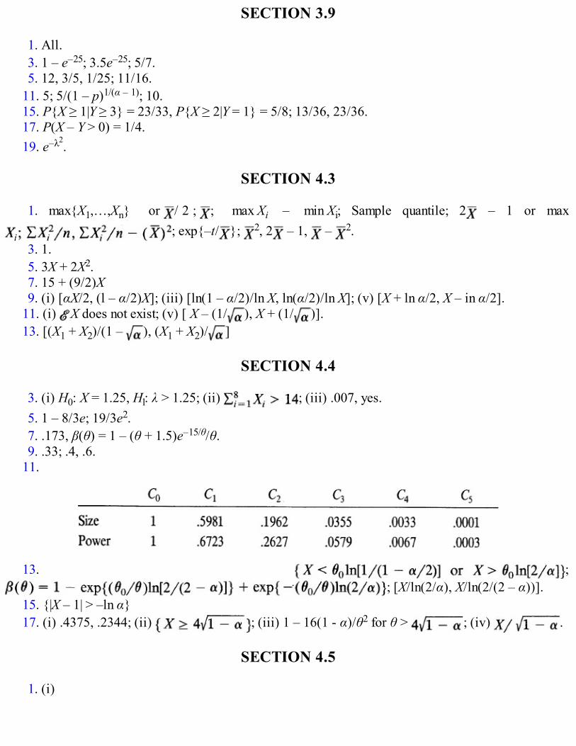
SECTION 3.9

1. All.3. 1 – e–25; 3.5e–25; 5/7.5. 12, 3/5, 1/25; 11/16.

11. 5; 5/(1 – p)1/(α – 1); 10.15. P{X ≥ 1|Y ≥ 3} = 23/33, P{X ≥ 2|Y = 1} = 5/8; 13/36, 23/36.17. P(X – Y > 0) = 1/4.19. e–λ2.

SECTION 4.3

1. max{X1,…,Xn} or / 2 ; ; max Xi – min Xi; Sample quantile; 2 – 1 or max ; exp{–t/ }; 2, 2 – 1, – 2.

3. 1.5. 3X + 2X2.7. 15 + (9/2)X9. (i) [αX/2, (l – α/2)X]; (iii) [ln(1 – α/2)/ln X, ln(α/2)/ln X]; (v) [X + ln α/2, X – in α/2].

11. (i) X does not exist; (v) [ X – (1/ ), X + (1/ )].13. [(X1 + X2)/(1 – ), (X1 + X2)/ ]

SECTION 4.4

3. (i) H0: X = 1.25, Hl: λ > 1.25; (ii) ; (iii) .007, yes.5. 1 – 8/3e; 19/3e2.7. .173, β(θ) = 1 – (θ + 1.5)e–15/θ/θ.9. .33; .4, .6.

11.

13. ; ; [X/ln(2/α), X/ln(2/(2 – α))].

15. {|X – 1| > –ln α}17. (i) .4375, .2344; (ii) ; (iii) 1 – 16(1 - α)/θ2 for θ > ; (iv) .

SECTION 4.5

1. (i)

(ii) = 17.51, Median 23.05.3.

5

7. (i)

SECTION 4.6

1. (i)

(iii) = 26.35 from frequency distribution and = 26.398 from sample observations.3. .5. ,

, or max(X1, X2) < 1 + }, [28.5, 116.3].7. (i) C = {|X| < θ0(1 – (1 – α)1/3)}; (ii) β(θ) = 1 – [1 – (θ0/θ)(1 – (1 (1 – α)1/3]3; (iii) /[l – (1 –

α)1/3].9. (i) ,

; (ii) , or , .

SECTION 5.2

1. 2 X,( X)2.3. 8/3.5. 2.4, .6,1/8.

9. 0.

SECTION 5.3

1. 2.3. (i) 2σ2; (iii) σ2/2; (v) σ2/n.5. 48, .025.7. 46/25.9. σ = σ2

2/(σ1 + σ22).

11. (ii) 1/2; (iii) [var(X) – var(Y)]/[var(X) + var(Y)].15. (n – m)/n.21. Sp

2.23. p(1 – p) and p/(1 – p)(n – 1)/n; np(l – 2p)2(l – p)/(n – l)2 and p(l – p)(1 – 2p)2/n.25. .

SECTION 5.4

1. Only in (ii).9. 500; 2000; 8000.

SECTION 5.5

1. {X|y} = 10/3 for y = 0, = 9/3 for y = 1; var{X|y;} = 14/9 for y = 0, = 2 for y = 1.3. 75 minutes.9. (i) Y/2, Y2/3; (iii) 2(6 – Y)/3, (6 – Y)2/2.

11. .19. Median of Y given X.

SECTION 5.6

1. (Y – X) = 1, {Y|x} = 1 + x.3. .5. (3X + 2)/(6X + 3), 8/75; (6X2 + 6X + 1)/18(2X + l)2.7. {X|Y} = 0, XY = 0.

13. (ab/2){sin θ – (θ cos θ)/2 – (θ2/6)sin θ}, ((ab)2θ2/12)sin2θ + [(ab)2/4][(θ/2)cos θ + (θ2/6)sinθ]2.

SECTION 6.2

5. –1/38.7. (i) P(Nn = k) = ((N – k + 1)/N)n – ((N – k)/N)n, Nn = , (Mn + Nn) = N + 1; (ii)

.

SECTION 6.3

3. .0432.5. (i)p = 1 - σ2/μ; n = 25,p = .4; P(X ≥ 10) = .2447; (ii) No.7. 8; 3; 6; 4.9. .1133, no.

11. .0197, (.0197)4.13. n = 13 or 14.15. .1091, 9.25. ;

.27. (i) .65; (iii) .6, .012; (v) 1.29. (i) .4; (iii) [0, .5]; (v) .9568.31. [.18, .62].33. P-value = .5034, power at .3, .4, .6, .7 respectively .416, .128, .128, .416.35. P-value = .063.37. (i) none; (ii) {X ≤ 2 or X ≥ 10}; (iii) { X ≥ 10}; (iv) {X ≤ 18 or X ≥ 32}.39. ≥ .0002 (for two-sided case).41. P-value = .3436.43. P-value = .7538.45. P-value = .0004.47. X1X2/X12.

SECTION 6.4

1. 1/210; 185/210.3. 7/9; 3, 6.5. p = 1/42, yes.7.

11. No.13. .29, 1740.17. P-value = .1002.19. P-value = 1.0.21. P-value = .1849.23. P-value = .5447.25. P-value = .31.

SECTION 6.5

1. .067; .7209; 4.3. .00001.5. 1 – [1 – 3p(1 – p)]n–1 n = 2.7. 1/4; p/(p + 3p).9. 1/2x+1, x = 0,1,…n — l,P(X = n) = 1/2n.

11. (1 – p)k – 1, .6561; 9 or 10.13. Geometric with p2; Geometric with 1 — (1 — p)2.

15. 2/3.17. .00032; .0044, .0149.19. .4929; 3.38.23. P(X = 1) = 1 – p, P(X = k) = p2(1 – p)k – 2, k ≥ 2; 2; 2(1 – p)/p.

SECTION 6.6

1. .018; .195; .785.3. λ = 2.2; .072; .244; .975.5. .323; .135; .406.7. .176; .440; .384.9. (ii) .67 vs. .866; (iii) .916, .101.

11. P(X ≤ 1|λ = 2) = .406; P(X ≤ 1|λ = 4) = .092; P(X ≤ 1|λ = 8) = .003.13. .15. [λ].17. (ii) [.86,29.14], [2.1,11.9].19. (i) Poisson (λp); (ii) eλ(1 – p)[λ(l – p)]x – k/(x – k)!, x = k, k + 1,… .

SECTION 6.7

1. .1055.3. .008; .115; .45.5. .0073.7. .042.

11. .13. {X1|x2} = (n – x2)n1/(N – n2).

15. (i) 1/4, 1/2, 1/4; (ii) 0, 1/2, 1/2; (iii) .

SECTION 6.8

1. Binomial (10, 1/5), 2, .006, 4.3. .442; .251; .934.5. .2529; 9.7. Poisson (k + 1); .908.

11. Poisson (λp);λp.15. P-value = .377.17. P-value = .0934.

SECTION 7.2

1. .67, .27, .6; .3.3. (ℓ + 1 )/(k + ℓ + 1).5. f(x) = 1 on [c - 3d/c, c + 3d/c]; [(3d/c) – l/2]/2c for 6d > c.7. (i) 1/2, 1/5; (iii) 1/3, 4/15.9. (i) 1,1/9; (ii) .0774; (iii) ≤ 4/9.

11. 1/2.13. (1/4) + (3/16)ln3 = .456.15. 2(1 – x), 0 ≤ x ≤ 1, and 2y, 0 ≤ y ≤ 1; 1/y, 0 ≤ x ≤ y.17. 7/9.19. f(x, y, z) = 6, 0 ≤ x ≤ y ≤ z ≤ 1; fX, Y (x, y) = 6(1 – y), 0 ≤ x ≤ y ≤ 1, fY, Z(y, z) = 6y, 0 ≤ y ≤ z ≤ 1; fX,

Y(x, z) = 6(z – x), 0 ≤ x ≤ z ≤ 1.21. 4/9.

SECTION 7.3

1. .3. 9!/310.5. 9.

SECTION 7.4

1. eλt; eλt1 – eλt2.3. P(Y ≥ n/2), Y binomial with p = e–t/λ; p = .6065.5. Process 1: c + ,8647d; Process 2: 1.5c + .6363d; Process 3: 2c + .6321d.7. 1 – e–1/λ.9. $658.33.

11. .8646, .5955, .6066.13. .981; .228.15. .003,.458.17. .19. 25. for ± > 2.

SECTION 7.5

3. 1/6; .3221; .2007.5. .4449.7. ± = .08, ² = .72.9. f{p|k} = pk + ± – 1(1 – p)n – k + ² – 1/B(k + ±, n – k + ²), 0 < p < 1.

11. B(p + ±, q + ²})/B{±, ²).

SECTION 7.6

1. (i) .7054; (iii) .8968; (v) .2362; (vii) .1949.3. (i) .3707; (iii) .5899; (v) .6293.5. (i) 4.28; (iii) .38; (v) 2.67; (vii) .67.7. .1151; 51.6.9. .6247.

11. .0062, .1815, yes.

13. (i) .0618, (ii) 628, 664.15. 8 oz.17. σ = .0667 oz.19. 2.28 percent; 81.2.21. μ = 95 + (σ2/10)ln{(P2 + P3)/(P2 – P1)}.23. k–1/2 (2π)(1 – k)/2; c = k1/2(2π)(k – 1)/2; 0, 1/k.

SECTION 7.7

1. (i) , 0, 0, 4/3, 4/3, 1/2; (iii) , –5, 0, 16/3, 4/3, –1/2.3. 4, 15/4,16, 9, -3/4; normal (6 - 9x/16, 63/16); .3191.5. (i) .4782; (ii) .1175; (iii) 1.5174.7. Normal (0, C/2(AC – B2)) and normal (0, A/2(AC – B2)); B = 0, .

SECTION 7.8

1. 1/3, 1/6, 1/18, 7/180, 1/4, 1/2.3. P(Y = y) = l/(n + l), y = 0, 1,…,n.

11. 2.5, .0183.13. Normal (.8x + 5,2.54), 22.6, .5211.15. l/2x + 1, x = 0, 1, 2…; .4859.17. 36.28; 8.04, 41.96; .8664 vs. .5556.19. 2.5, 5, 7.5; (15!/(6!4! 5!))(l/6)10(2/3)5.21. 53 .

SECTION 8.2

1. .

3. .5. .7. .9. .

11. (i) 25/144, 60/144, 46/144, 12/144, 1/144 for x = 0, 1,…,4; (iii) 46/144, 72/144, 26/144 for x =0, 1, 2.

13. Binomial (n1 + n2, p).15. 1 – y/2, 0 ≤ y < 2.17. .23. .

SECTION 8.3

1. (1/|a|)f((y – b)/a).3. .

5. .9. .

19. .21. 1/2, 0 < u + v < 2, 0 < u – v < 2.

SECTION 8.4

1. (i) 1 – |y|, |y| < 1; (iii) 1/2, 0 < x < 1, and l/2x2 for x ≥ l.5. 1/(1 + y)2, y ≥ 0.7. P(X1 + X2 = k) = (k – l)/N2, k = 2,…,N and = 1/N for k = N + l,…,2N.

17. fz(z) = 2z2 – 2z3/3, 0 < z < 1, = 4[(1 – z)/2 + 1/3 + (z – l)3/6], 1 < z < 2; No.

SECTION 8.5

1. .

3. P(X(1) = x) = 1/12, 1/12, 4/12, for x = 1,2,3.5. .0989.9. [(n – l)/λ]e–r/λ(l – e–r/λ)n – 2, r > 0.

11. .13. .15. .17. [X(5), X(10)].19. 29.6; [27.9,30.4] or [28.6,30.8].21. 9; 7; 11.23. P-value = .3214.25. P-value = .754.

SECTION 8.6

1. sP(s); P(sm); skP(sm).3. (i) ps/(1 – s(l – p)) |s| ≤ (1 – p)–l; (iii) [e–λ/(1 – e–λ)](esλ – 1); (v)f(sθ)/f(¸) |s| ≤ l.9. (i) Binomial (n, 1/2); (iii) P(X = k) = pk/[ln(l – p) –k], k = 1,2,… .

15. Xk = (k + 1)!.19. (i) Gamma (n, λ); (iii) Gamma .23. M(s1, s2) = [(es2 – l)/s2s1

2](l – es1 + s1es1) + [(es1 – l)/s1s2

2](l – es2 + s2es2).25. 2[s1s2(s1 + s2)]–1 {s1es1(es2 – 1) – s2(es1 – 1)}.

SECTION 8.7

1. (i) .98; (iii) 2.086; (v) 1.74.3. (i) .01; (iii) 14.067; (v) 3.94, 18.307.

5. (i) 8.45; (iii) 3.86; (v) .153.7. [.082, .108].9. [206.1,218.7].

11. [9.53,21.59].13. 18.15. [6.21,7.39].17. t0 = 2.69.19. [.49,1.67].21. [–.04,1.44].23. t0 = 1.609.25. t0 = 6.39.27. t0 = 1.27.29. t0 = 2.36.31. t0 = 2.28.33. v0 = 15.36.35. f0 = .7398, yes.37. f0 = 1.25, no.

SECTION 8.8

3. (i) P(Y = 1) = 1 – F(0), P(F = –1) = F(0); (iii) P(Y = c) = 1 – F(c), P(Y = –c) = F(–c) and fY(y) =fx(y) for |y| < c.

5. (iii) 1/(1 – X); (v) h(X) = , 0 < X < 1 and = ), 1 ≤ X ≤ 2.9. 2/3.

11. z3e–z/λ/6λ4, z > 0.13. (i) (18t – 12t2)/5, 0 < t < 1; (ii) 12t/(1 + t)4, 0 < t < 1.15. σ2(π – 2)/2.17. (i) Binomial (t, 1/n).19. .375, .5625, .6797, .7617, .8218, .8664, .8999, .9249, .9437 for n = 2, 3 …, 10 respectively.21. (i) none; (ii) [32,100, 47,600].23. [1, 33]; P-value = .5274.29. t0 = –2.04.31. t0 = .93; [–5.78, 11.98].

SECTION 9.2

3. P(X = β) = 1.

SECTION 9.3

1. (i) No; (iii) No; (v) Yes.3. .5098.5. .0021; .9958; .9236.7. 271.

9. z0 = —3.6.11. z0 = 2.42.13. .5762; 385.15. σ = 60.79.17. (i) .33, .1922, .0409, 0 + , 0 + , limit 0.23. Normal (p1 – p2, [p1(1 – p1) + p2(1 – p2)]/n); normal (pl – p2, [p1(1 – p1) + 2p1p2 + p2(l – p2)]/n).

SECTION 9.4

1. z0 = –2.27.3. .8462; .9989.5. 84.7. 0+; .0014.9. 233.

11. .0357 (normal), .034 (Poisson).13. .0104, .5693; .0043.15. .17. Exact .2642, Poisson .264, normal .3085.19. Binomial .0103, normal .0096.

SECTION 9.5

3. ; normal (2p1 – 1, [4p1(1 – p1)/n]).5. if Xi = 0, Yj = 0 otherwise.7. .9. .

13. No.

SECTION 9.6

1. [10.0035,10.0165], No.3. [66.8, 69.6].5. [12.0, 12.06].7. [.32, .48].9. [.3967, .4783].

11. 96 or 97; 81.13. 34.15. [29.8,46.2]; [30.1,45.9].17. [–.24, –.16].19. [–.138, .018].21. [7.25,15.75].23. ; [.258, .408].

25. .

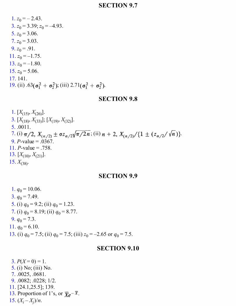
SECTION 9.7

1. z0 = – 2.43.3. z0 = 3.39; z0 = –4.93.5. z0 = 3.06.7. z0 = 3.03.9. z0 = .91.

11. z0 = –1.75.13. z0 = –1.80.15. z0 = 5.06.17. 141.19. (ii) .63 ; (iii) 2.71 .

SECTION 9.8

1. [X(15), X(26)].3. [X(18), X(33)]; [X(19), X(32)].5. .0011.7. (i) ; (ii) .9. P-value = .0367.

11. P-value = .758.13. [X(10), X(21)].15. X(38).

SECTION 9.9

1. q0 = 10.06.3. q0 = 7.49.5. (i) q0 = 9.2; (ii) q0 = 1.23.7. (i) q0 = 8.19; (ii) q0 = 8.77.9. q0 = 7.3.

11. q0 = 6.10.13. (i) q0 = 7.5; (ii) q0 = 7.5; (iii) z0 = –2.65 or q0 = 7.5.

SECTION 9.10

3. P(X = 0) = 1.5. (i) No; (iii) No.7. .0025, .0681.9. .0082; .0228; 1/2.

11. [24.1,25.5]; 139.13. Proportion of 1’s, or .15. (Xi – Xj)/n.

17. [24.2, 31.8]; z0 = –2.1.19. z0 = 3.65; [2.9, 7.5].21. [–.17, –.03]; z0 = –2.18.23. [20.6,40.3]; P-value = .6170; P-value = .401.

SECTION 10.2

3. No, yes.5. .7. (i) ; (iii) ; (v)

{X(1), X(n)}, (vii) ; (ix) .

SECTION 10.3

1. (n – X)/n; (2X – n)/n.3. (i) Not possible; (ii) (T – b)/a.5. .7. pX, r( 1 – p); p2X2 + p2X – pX.9. 6.71, .96.

11. 2.04, 1/50.13. 3 – 2b.15. 3 .19. .21. .23. .25. sufficient; neither is best.

SECTION 10.4

1. (ii) (1 – ); (iii) (n – 1 )S2/n.3. X/p.5. .7. .9. .

11. , or proportion of Xi’s > t.

SECTION 10.5

1. X(n).3. l(xi) = Number of xi in sample, = l(x3)/(l(x1) + l(x3)) if l(x1), l(x3) > 0, if l(x1) = 0 = l(x3) any

value in (0,1); if l(x1) = 0, = 1; if l(x3) = 0, = 0.

5. .

7. .

9. where are mles; (iii) exp.

11. density and distribution function of standardnormal.

13. .15. .

SECTION 10.6

1. (ii) (k + 1)/(n + 2); (c) l/6(n + 2).3. xe–θx; 1/X.7. .9. .

11. .13. (ii) ; (iv) = 1302.71, θn = 1303.48, risk ratio 1.008.15. .17. .104.19. 4601.8; .8291.

SECTION 10.7

1. .3. where λ1 and λ2 are solutions of and

.5. [X/(l – λ1), X/(l – λ2)] where and (λ1 + λ2 – 1)2 = λ1λ2.7. .9. .

11. .17. h(θ|x) = [(θ – x)/4]exp(–(θ – x)/2), 0 < x < θ.

SECTION 10.8

1. (a) (i) and ; (iii) X(n) and X(n); (b) [(3n + l)/3n]X(n) and .3. Yes, yes.5. No.7. .

11. 2X; No.13. .15. Choose c from α = cn – 1[n – (n – l)c], ((R/c) – R) = [(n – 1)/(n + 1)]θ [(1 – c)/c], (α–1/nX(n) –

X(n)) = (α–1/n – l)nθ/(n + 1).17. ; .5625 and [.52, .62].19. [(n + α)/(n + α – l)]max(a, x1, …, xn); 21/(n + α)max(a, x1, …, xn); [max(a, x1, …, xn) , α–1/(n +

α)max(a, x1, …, xn)].21. r/n.23. .

SECTION 11.2

1. {∑ Xi, ≥ k}.3. {X ≥ k}.5. {X ≥ k}.7. {|X| ≤ k}.9. .

11. (i) {X(1) ≥ θ0 + (l/n)ln(1/α)}, {X ≥ 1 – α}, {X(1) ≥ θ0α–1/n}, ; (ii) exp{n(θ1 – θ0 – (l/n)ln(1/α))}, 1 – (1 – α)θ1, α

(θ1/θ0), .

SECTION 11.3

1. {∑Xi ≥ k}, P-value = .0539.3. {∑Xj ≥ k}.5. { ≤ k}.7. (i){∏Xj ≥ k}, (ii) {∏Xj ≥ k}; (iii) {X(1) ≥ k).

SECTION 11.4

1. (i) {X(n) ≥ N0}; (ii) {X(n) > N0 or X(n) < c}.3. { ≤ c1 or ≥ c2}.5. {X ≤ c1 or X ≥ c2}.7. (i) or ; (ii)

.9. .

SECTION 11.5

1. w+ = 29, t0 = 1.424.3. w– = 49, t0 = –3.76.5. w– = 37.5.7. W+ = 111.9. (i) P-values of sign, Wilcoxon and Mests respectively .8238, .2802, between .3 and .4.

SECTION 11.6

1. tx = 130.5.3. tx = 82, R = 8.5. tx = 33.5.7. R = 11.9. R = 23.

11. .

SECTION 11.7

1. .3. q0 = 8.41.5. q0 = 8.41.9. q0 = 2.71.

SECTION 11.8

1. Dn = .24.3. Dn = .1946.5. Dn = .2321.7. Dn = .3444.9. Dn = .3715.

SECTION 11.9

1. (i) t0 = 1.182, (ii) t0 = 1.13; (ii) t0 = –4.407.3. rS = .8571, τ = .7857.5. rS = .8607, τ = .7143.7. rS = –.3482, τ = –.2857.9. r = .5647 and t0 = 2.903, rS = .5135.

SECTION 11.10

1. |X| > c1 or |X| < c2.3. {X ≤ k}.5. {∑Xi < k}.7. {X(1) > k}.9. {∑Xi < c1 or ∑Xi > c2}.

11. .15. w+ = 146.5.17. tx = 34, r0 = 7.

19. r0 = 6.21. tx = 173.23. q0 = 7.356.25. q0 = .669.27. D20 = .104929. r = –.9228.31. r0 = 21.33. rS = .80, τ = .67.

SECTION 12.2

1. q0 = 15.41.3. (i) q0 = 6.7; (ii) q0 = 6.3.5. q0 = 3.54.7. q0 = 21.81.9. q0 = 219.1.

SECTION 12.3

1. q0 = 217.6.3. q0 = 256.4.5. q0 = 58.7.7. q0 = 28.47.

SECTION 12.4

1. q0 = 15.74.3. q0 = 11.46.5. q0 = 5.25.

SECTION 13.2

1. f = 12.17.3. f = 56.45.5. f = 16.46.7. f = 49.13.

SECTION 13.3

1. μB > μC, μB > μE, μD > μC, μD > μE.3. μ4 > μ3 > μ1 > μ2.

5. .

SECTION 13.4

3. (i) fMethods = 1.0, finstructors = .45; (ii) fMethods = 1.08, finstructors = .48, fI = 1.73.5. fvariety = 24.00.7. fstrains = 48.61; μA > μC > μD, μB > μC > μD.9. μD > μC > μA, μD > μC > μB.

11. t0 = 5.34; fTreatments = 28.66.

SECTION 13.5

1. q0 = .1719, h = .2598.3. h = 21.42, f = 93.52; μ1 < μ3, μ1 < μ4, μ2 < μ4.5. h = 37.52; μA < μD, μA < μE, μA < μF, μB < μE, μB < μF, μC < μF.

SECTION 13.6

1. f = 9.3. f = 21.775.5. w = .8443, f = 37.996.7. w = .9665, f = 27.0625.

SECTION 13.7

1. f = .3747.3. (i) f = 46.34, μA > μC > μD, μC > μB; (ii) fStimuli = 38.27, fSubjects = 1.53, μA > μC > μD > μB; (iii) f =

13.38.5. f = 28.82, μ1 < μ2, μ1 < μ3; h = 22.06, μ1 < μ2, μ1 < μ3.7. fFields = 3.45, fSex = 1.72, fI = 13.09.9. w = .706, f = 14.83.

11. w = .4, f = 6.4.

INDEX

Additive factors, 824Additivity property, 28Analysis of categorical data, 780Analysis of variance: one-way, 802

and t-test, 804two-way, 822two-way with interaction, 822

Approximating distributions, 556Approximating mean and variance, 267Association analysis, 762Asymptotically normal, 570Asymptotic distribution, of rth order-statistic, 616

of sample moments, 579of sample quantiles, 616

Bayesian confidence interval, 700estimation, 684, 689, 693

Bayes' rule, 51, 52, 128, 685Bernoulli:

probability function, 304random variable, 304trials, 305

Bertrand's paradox, 395Beta distribution, 417

mean and variance, 418moments, 417relation with binomial, 330, 419, 500relation with F-distribution, 488

Biased estimate, 652Bias of estimate, 652Bimodal, 165Binomial:

coefficient, 37distribution, 307expansion, 37experiment, 305random variable, 307series, 360

Binomial coefficient, 37expansion, 37series, 360

Binomial distribution, 307approximation by Poisson, 372mean and variance, 313moment generating function, 517moments, 312–313, 510probability generating function, 511relation with beta, 330, 419, 500

Bivariate normal, 433, 436circular, 436moment generating function, 517

Black Jack, game of, 77Borel law of large numbers, 314, 559

Capture-recapture method, 335Cassell v. Texas, 145Cauchy distribution, 471, 485

moments, 440Cauchy-Schwarz inequality, 251Census, 68

Central limit theorem, 560, 568Chebyshev inequality, 161, 171, 314, 424, 596

and confidence intervals, 203, 264is sharp, 163

Chi-square distribution, 411, 522, 527as approximation to negative binomial, 560mean and variance, 416normal approximation, 528as square of normal, 448

Chi-square test:of goodness of fit, 624, 747, 749of homogeneity, 624of independence, 791

Class interval:boundaries, 232frequency, 231

Combinations, 37Completely randomized design, 801, 813, 835Composite hypothesis, 214, 716Concordant pair, 767Conditional:

density function, 126distribution function, 123, 127expectation, 280probability, 44probability function, 122

Confidence:bounds, 198estimation, 188, 694level, 198

Confidence interval, 198, 694Bayesian, 700and central limit theorem, 596and Chebyshev inequality, 204, 264using Chebyshev inequality, 203, 596, 597and hypothesis testing, 224large sample, 595length, 199minimum level, 198shortest length, 697simultaneous, 817, 837

Consistent estimate, 196mean square, 595

Consistent sequence, 179Contingency table, 784, 791

testing independence, 791Continuity correction, 582Continuity theorem, 557Continuous type distribution, 89, 95Convergence in probability, 591Convolution:

of density functions, 479of probability functions, 480

Correlation:coefficient, 253, 294, 724, 762and independence, 436, 763

Correlation coefficient, 253, 294, 724, 762interpretation, 254, 262sample, 266, 639

Countable additivity, 28Counting rules, 33Covariance, 249

sample, 639Craps, game of, 66, 367

Critical region, 212, 215best, 709

Data, 1Degenerate random variable, 299Density function, probability, 89Dirichlet distribution, 44Discordant pairs, 767Discrete distributions, 89, 93Discrete models, 297Discrete type random variable, 89Discrete uniform distribution, 298

probability generating function, 511Distribution:

conditional, 122, 125–128posterior, 685prior, 685of sample mean, 522, 569of sample range, 493–494

Distribution function, 90continuous type, 94discrete type, 89empirical (= sample), 234, 264, 277, 660, 681, 705, 755jump point of, 93method of, 445ogive estimate of, 236of a random variable, 90, 445of a random vector, 445size of jump, 93

Double exponential (= Laplace) distribution, 483

Efficiency, relative, 193Election reversal, probability, 345Empirical (= sample) distribution function, 234, 264, 277, 660, 681, 705, 755Error:

in estimation, 197, 276Type I and Type II, 212, 215

Estimation:bias, 191biased, 191point and interval, 188–189unbiased, 191

Event(s), 11disjoint = mutually exclusive, 12elementary, 18independent (pairwise), 56mutually independent, 58null, 26

Exchangeable random variable, 292Expectation:

conditional, 280mathematical, 150

Expected value = mean = mathematical expectation, 150frequentist interpretation, 153of a function, 245of product, 245of sum, 245

Experiment:independent, 61random = statistical, 4

Exponential distribution, 404characterization, 405lack of memory, 405mean and variance, 404

moment generating function, 517relation with Rayleigh, 449relation with uniform, 451relation with Weibull, 408

Factor(s), 808levels, 809

Failure rate (= hazard) function, 407, 422decreasing, 416increasing, 416, 442increasing on average, 442

F-distribution, 484, 488, 530and beta, 488and chi-square, 484mean and variance, 531, 553

Finite population correction, 261, 345, 600Fisher-Irwin test, 349, 609Fitting a distribution:

binomial, 632, 754exponential, 633, 753normal, 629, 751Poisson, 628, 750uniform, 237, 630

Fixed effects, 813Frequency, 15

class, 231interpretation of probability, 23relative, 15, 276

Friedman test, 855distribution, 855

F-statistic, 484, 530F-test, robustness, 812

Gallup poll, 72Gamma distribution, 408

mean and variance, 410moment generating function, 517moments, 409relation with Poisson, 413

Gamma function, 398Gap estimate, 302Generating functions, 505

moment, 511probability, 506

Genes and genotypes, 386, 670Geometric distribution, 354, 355

characterization, 369lack of memory, 358mean and variance, 357moment generating function, 511

Geometric probability, 394Goodness of fit tests:

Chi-square, 626, 748–749Kolmogorov and Smirnov, 754Hardy-Weinberg principle, 670, 684, 752–753, 775

Hazard function, 407Histogram, 95, 231

estimate of density, 234, 295relative frequency, 232, 234

Hypergeometric distribution, 336approximation by binomial, 341–342, 351approximation by Poisson, 379mean and variance, 334

Hypothesis:

alternative, 211, 214composite, 214, 716nonparametric, 214null, 210, 214parametric, 214simple, 214simple vs. simple, 709statistical, 209, 214test of, 214

Identical distribution, 173Improved confidence interval, for binomial p, 319–320

for Poisson λ, 378Increasing failure rate, 416

on the average, 442Independence, and correlation, 763

mutual, 58pairwise, 56of random variables, 139–140

Independent experiments (= trials), 61Interaction effects, 823Interquartile range, 164Interval estimate, 188

Joint:density, 106, 120distribution, 107, 120, 134moment generating function, 517probability function, 106, 120probability generating function, 517

Jump, 93size of, 93

Jury discrimination, 145

Kendall’s coefficient of concordance, 858, 864and Friedman test, 858and Spearman’s rank correlation, 864

Kendall’s tau, 767–768asymptotic distribution, 769comparison with Spearman’s test, 770null distribution, 769probability generating function, 519test, 768treatment of ties, 769

Kolmogorov-Smirnov statistics, 755, 758Kolmogorov-Smirnov test, 754, 755, 758

comparison with chi-square, 760confidence bands, 759null distribution, 756

Kruskal-Wallis test, 848and analysis of variance, 847asymptotic distribution, 848and Mann-Whitney Wilcoxon test, 847, 853null distribution, 848ties, 848

k-Sample problems, 801nonnormal case, 842, 854normal case, 802, 822related samples, 854

Laplace (= double exponential) distribution, 483moment generating function, 520

Large numbers:Borel law of, 314, 559

law of, 274Large sample:

estimation, 597hypothesis testing, 606

Law of large numbers, 274Likelihood, 223

equation(s), 674function, 673, 686ratio, 219, 224, 720

Likelihood ratio test, 720for homogeneity of proportions, 791for independence, 798large sample distribution, 725and Neyman-Pearson lemma, 725and sufficiency, 727

Linear combinations, 257Linear regression, 294Linear unbiased estimation, 664

minimum variance, 664Literary Digest poll, 75Lognormal distribution, 471

moment generating function, 520moments, 520

Loss function, 689

Main effects, 823Mann-Whitney-Wilcoxon test, 737

asymptotic distribution, 738comparison with other tests, 744null distribution, 738, 747treatment of ties, 738–739

Marginal:density, 120distribution, 134joint, 120probability function, 120

Mathematical expectation, 150Maximum likelihood: estimate, 337, 674

generalized, 693invariance, 680method, 671and minimum chi-square, 754principle, 674and sufficiency, 679

Maxwell distribution, 412, 429mean and variance, 416

Mean, 150sample, 176

Mean absolute deviation, 156Mean square error, 192, 653Measures of association, 762

Kendall’s tau, 767–768Spearman’s rank correlation, 764

Median, 164, 170sample, 179

Median test, 347extended, 843

Method of distributions, 445Method of moments, 665–669Minimal sufficient statistic, 643, 649Minimum chi-square:

estimate, 748and maximum likelihood, 754method, 748

Mode, 165sample, 179

Model(s), 1continuous, 390discrete, 292mathematical (= deterministic), 2nondeterministic (= stochastic), 1, 2nonparametric, 187parametric, 186

Moment(s): absolute, 151about c, 151central, 151of order k, 151

Moment generating function, 511bivariate, 521continuity theorem, 557differentiation, 512expansion, 512limiting, 556and moments, 512–513multivariate, 517of sum, 516uniqueness, 515

Most powerful test, 709and Neyman-Pearson lemma, 709uniformly, 716–718

Most probable:number of successes, 330value, 165

Multinomial:coefficient, 38distribution, 381expansion, 38

Multinomial distribution, 381covariance, 385as limit of multivariate hypergeometric, 382mean and variance, 385moment generating function, 517

Multiple comparisons: in nonparametric one-way analysis of variance, 850in nonparametric two-way analysis of variance, 860in parametric one-way analysis of variance, 817in parametric two-way analysis of variance, 837

Multiplication rule, 47Multivariate distributions, 105

bivariate normal, 433, 436hypergeometric, 380moment generating function, 517multinomial, 381Poisson as limit of multinomial, 383probability generating function, 517

Negative binomial distribution, 360approximated by Poisson, 379, 557mean and variance, 362moment generating function, 517probability generating function, 511relation with binomial, 361

Neyman-Pearson lemma, 709and likelihood ratio test, 725and sufficiency, 716

Nonparametric:family, 185model, 187

Normal approximation: to binomial, 560

to chi-square, 560to integer-valued random variables, 579to Poisson, 558, 560, 575

Normal distribution, 421–422and Chebyshev inequality, 424mean and variance, 421moment generating function, 517moments, 440, 514standard, 421tail probability, 426

Null event, 26

Odds, 23ratio, 636

Ogive estimate, 236One-way analysis of variance, 802

table, 811and t-test, 804

Order of magnitude, 370Order statistic(s), 488

distribution, 491sufficiency, 648

Pairwise independent:events, 56random variables, 143

Parameter, 172, 186of distribution, 186as index, 186set, 186

Parametric:family, 185model, 186

Pareto distribution, 416mean and variance, 416

Partition:by random variable, 82by sufficient statistic, 649

People v. Collins, 65Permutation, 36Pivot, 695–697Point estimate, 189Point estimation, 188Poisson distribution, 369–370

approximation by normal, 558–560as limit of binomial, 372as limit of hypergeometric, 379as limit of negative binomial, 379mean and variance, 374moment generating function, 517probability generating function, 511relation with gamma, 413

Polya’s urn model, 50Population, 6, 36, 173Population distribution, 173Posterior distribution, 685Power function, 216Predictor:

best, 289, 292best linear, 294

Prior distribution, 685improper, 691noninformative, 691

Probability, 17

additivity, 28axioms, 15, 17conditional, 44density, 89distribution, 82, 89, 90frequency interpretation, 23function, 89generating function, 506geometric, 394histogram, 95integral transformation, 458–459model, 22multiplication rule, 47prior and posterior, 51, 685sample, 68space (= system), 22subadditivity, 28subjective interpretation, 23tail, 90, 159total, 49Type I and Type II error, 212uniform assignment, 18, 38

Probability generating function, 506differentiation, 506and moments, 506–507multivariate, 517of sum, 508uniqueness, 508

Quantile:confidence interval, 617estimation, 497, 618limiting distribution, 616population, 164, 496sample, 497, 616test of hypothesis, 500, 621

Quartile, 164first and third, 164

Random, 22, 391digits, 70effects, 813experiment, 4phenomenon, 2

Randomized block design, 834Randomized response model, 666, 683, 706Random sample, 67, 173

from a distribution, 171from finite population, 67, 174, 260, 299, 337, 599from an infinite population, 171simple, 67

Random variable(s), 82continuous type, 89, 95density function, 89discrete type, 89exchangeable, 292functions of, 443independent, 139, 140, 143induced distribution, 82infinite sequence, 179partition induced by, 82probability function, 89standardized, 158symmetric, 101

uncorrelated, 253Random vector, 85

continuous type, 106discrete type, 106functions of, 443joint distribution, 106

Range, 493, 551distribution of, 493

Rayleigh distribution, 408, 411mean and variance, 416

Regression function, 286Relative efficiency, 193Relative frequency, 276, 314Reliability, 58, 60Risk function, 689Round off error, 19, 98, 391, 561, 761Run(s), 740

distribution of number of, 747length of, 740

Runs test, 741asymptotic distribution, 742comparison with other tests, 744null distribution, 742for randomness, 744ties, 741

Salk vaccine, field trial, 584, 609Sample, 6

cluster, 71correlation coefficient, 266covariance, 265distribution function, 234mean, 176median, 179mode, 179moments, 177quartiles, 497, 616range, 493, 551space, 9standard deviation, 176statistic, 176stratifield, 71variance, 176, 266

Sample size, 72, 276, 535, 541, 549, 561, 600, 606, 609, 615Sample space, 9

continuous, 11discrete, 10

Sampling from a normal distribution, 522distribution of sample variance, 522independence of and S2, 522unbiased estimate of σ, 525

Sampling with replacement, 35, 69, 337, 364–365Sampling without replacement, 35, 36, 69, 303, 337,364–365Set function, 17Shortest length, confidence interval, 697Sigma field, 15

Borel, 21Sign test, 323, 325Simultaneous confidence intervals:

in one-way analysis of variance, 817in two-way analysis of variance, 837

Spearman’s rank correlation coefficient, 764–765asymptotic distribution, 765

comparison with other tests, 770null distribution, 765ties, 765

Standard deviation, 157sample, 177

Standardized random variable, 158Statistic, 176Statistical experiment, 4Statistical inference, 1Statistical regularity, 2Stem-and-leaf plot, 230Stirling’s approximation, 401Stochastic:

experiment, 2model, 1

Stochastic ordering, 736Student’s t-distribution, 483

mean and variance, 553Subpopulation, 36Substitution principle, 497, 664Sufficiency, 641

of order statistic, 648and unbiased estimation, 654, 657, 660

Sufficient statistic, 642factorization criterion, 645minimal, 643, 649

Survival:analysis, 407, 415function, 407, 442

Symmetric distribution, 101, 102, 171, 181, 183, 208System:

in parallel, 60in series, 58, 60

Tail probability, 90, 159Taxi problem, 300–301, 593, 656, 668t-distribution, 483, 522, 525, 530

and Cauchy, 525mean and variance, 553and normal, 527, 593t-test, 539, 540

Test, 214critical region, 214, 709of hypothesis, 214, 708level of significance, 215likelihood ratio, 720most powerful, 709Neyman-Pearson, 709size, 215statistic, 214uniformly most powerful, 217, 717–718

Test(s) of hypothesis, 209, 708of association, 762and confidence interval, 224frequency interpretation, 218of goodness of fit, 624, 626, 754of homogeneity, 780, 784of independence, 791, 793

Total probability rule, 49Transformations, method of, 464–465Trial(s), 61

independent, 61Trinomial distribution, 474Two sample tests, 735

Types of error, 212, 215

Unbiased estimate, 191, 652asymptotic, 595uniformly minimum variance, 653

Unbiased estimation, 191linear, 664and sufficiency, 654, 657, 660

Uncorrelated random variables, 253Uniform assignment, discrete, 18, 38

on an interval, 21two dimensional, 22, 391

Uniform distribution:characterization, 393continuous, 391discrete, 298mean and variance, 393moment generating function, 517and simulation, 460–461

Uniformly:minimum variance, 653most powerful, 716–718

Unimodal, 165

Variance, 156interpretation, 156, 157, 159, 162, 170of linear combinations, 258properties, 157, 159sample, 266of sum, 259

Waiting time, 364, 403Wald’s equation, 285, 511Weibull distribution, 406, 408, 412

and exponential, 408mean and variance, 416

Wilcoxon signed rank statistic, 520, 727asymptotic distribution, 729null distribution, 729probability generating function, 520

Wilcoxon test, 727–728comparison with other tests, 730for paired observations, 731as a test of symmetry, 731

World Chess Title Series, 386World Series of Baseball, 65, 363

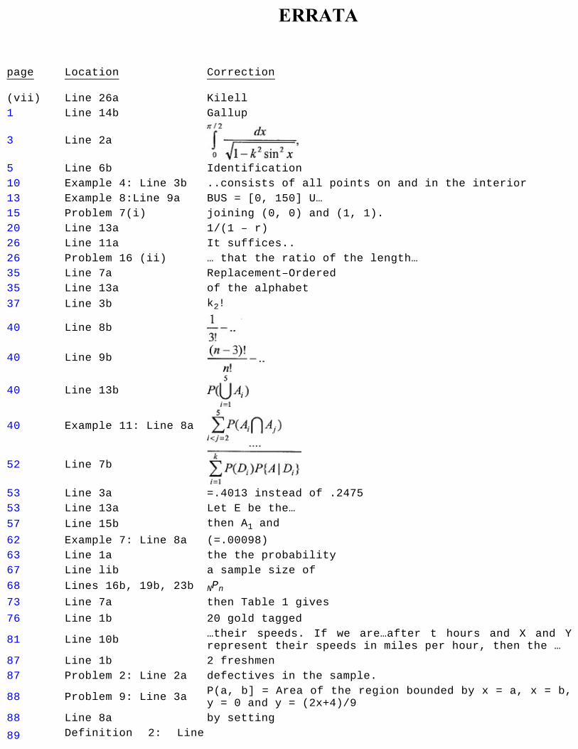
ERRATA

page Location Correction

(vii) Line 26a Kilell

1 Line 14b Gallup

3 Line 2a

5 Line 6b Identification

10 Example 4: Line 3b ..consists of all points on and in the interior

13 Example 8:Line 9a BUS = [0, 150] U…

15 Problem 7(i) joining (0, 0) and (1, 1).

20 Line 13a 1/(1 – r)

26 Line 11a It suffices..

26 Problem 16 (ii) … that the ratio of the length…

35 Line 7a Replacement–Ordered

35 Line 13a of the alphabet

37 Line 3b k2!

40 Line 8b

40 Line 9b

40 Line 13b

40 Example 11: Line 8a

52 Line 7b

53 Line 3a =.4013 instead of .2475

53 Line 13a Let E be the…

57 Line 15b then A1 and

62 Example 7: Line 8a (=.00098)

63 Line 1a the the probability

67 Line lib a sample size of

68 Lines 16b, 19b, 23b NPn

73 Line 7a then Table 1 gives

76 Line 1b 20 gold tagged

81 Line 10b…their speeds. If we are…after t hours and X and Y

represent their speeds in miles per hour, then the …

87 Line 1b 2 freshmen

87 Problem 2: Line 2a defectives in the sample.

88 Problem 9: Line 3aP(a, b] = Area of the region bounded by x = a, x = b,

y = 0 and y = (2x+4)/9

88 Line 8a by setting

89 Definition 2: Line

2a … on , and the distribution of x is specified…

91 Line 8a … function F…

97 Line 9a 0 < y < t0

99 Line 10b has “density” f

101 Line 7a and differentiable.

102 Problem 2(ii) x = 0, 1, 2,…, 15

103 Problem 8(ii) Add at the end: λ > 0.

104 Problem 12(i) F(x) = c{arctan x + π/2}

104 Problem 12 (ii) F(x) = 0, if x ≥ 1,

Problem 14: Line 3a the length of life (years) of …

105 Problem 20(i) P(X ≥ x) = e–λx

114 Lines 12a to 14a

116 Line 9a x ≥ 0, y ≥ 0

117Problems 7(iv) and

(v)x ≥ 0, y ≥ 0

118 Line 3b Drop (i), change (ii) to (i) and (iii) to (ii)

118 Problem 11: Line 2a 0<x<y<z<u<∞

119 Problem 20: Line 2b f(x)g(y)[1 + α(2F(x) – 1)(2G(y) – 1)]

120 Line 1b of X and Y are

120 Equation (3)The summation is over the remaining k - j xi’s other

than xi1, …, xij

129 Line 4a

129 Line 3b for |x| ≤ r and zero elsewhere

129 Line 5b for |x| ≤ r

129 Line 5a

130 Line 12a on using integration

134 Example 7: Line 4a f1 = cΔx

141 Line 1a Indeed,

142 Line 2a f (x, y) =

142 Proposition 1 Change f1, f2,…, fk to h1, h2,…, hk and f to h

146 Line 5a would ever appear

Lane 4b percent black

147 Problem 1 Replace ‘–’ by 0 in the table

148 Problem 9(v) f(x, y) = 1/(2x2y), 1 ≤ x < ∞, 1/x ≤ y ≤ x;

148 Problem 9(i)

148Problems 9 (iii) &

9(vii)0≤y<x<∞

150 Line 2b Suppose X is a

151 Line 3a If X is of …

157 Remark 4: Line 1a may be

159 Line 8b

164 Line 6b F is increasing

165 Line 10a unique maximum

166 Line 6a .175 .175 .146

166 Line 14a values are 4 and 5 … is bimodal.

169 Line 8b of .2 day.

170Problem 24(iv): Line

1a(α+β–1)!

172 Line 12b for t ≤ 0

173 Line 13a emphasize

176 Line 9a any function φ(X1, … , xn)

182 Problem 1(iii) 0 ≤ x ≤ 1

190 Example 2: Line 1b near θ/2 for 1arge n.

191 Line 8a EθT (X1,…, Xn)

195 Line 7b

198Definition 6: Line

3aF ∈

Line 4a = 1–α; 0<α̼1.

199 Line 6a confidence interval…

199 Example 6: Line 7a Lower Confidence

207 Line 3a .689 instead of .589

210 Line 9b …, X2 = x2, …

211Paragraph above

Table 1…from the table below if…

212 Line 7a .3438 instead of .348

214 Line 14a writing H1:

217 Line 2a 1 – Pθ (Type II error)

224Proposition 1: Line

3aC = { (x1, …, xn): θ0

224 Line 4a test of H0: θ = θ0.

224 Line 15b …yields the acceptance…

224 Line 15b [l( ), u( )] yields

225 Line 12a

225 Example 8: Line 2b Since for example,

226 Line 20b is observed then

228 Problem 8: Line 2a

230 Line 14b graphical form

242 Problem 7: Line 3a 3(θ–x)2/(2θ3)

246 Line 10b

246 Line 9a

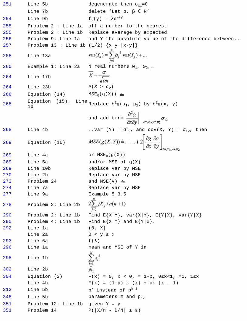
251 Line 5b degenerate then σxx=0

Line 7b delete ‘Let α, β ∈ R’254 Line 9b f2(y) = λe

–λy

255 Problem 2 : Line 1a off a number to the nearest

255 Problem 2 : Line 1b Replace average by expected

256 Problem 9: Line 1a and Y the absolute value of the difference between..

257 Problem 13 : Line 1b (1/2) {x+y+|x-y|}

258 Line 13a

260 Example 1: Line 2a N real numbers ω1, ω2,…

264 Line 17b

264 Line 23b P(X > c2)

268 Equation (14) MSEθ(g(X))

268Equation (15): Line

1bReplace δ2g(μ1, μ2) by δ

2g(x, y)

and add term

268 Line 4b ..var (Y) = σ22, and cov(X, Y) = σ12, then

269 Equation (16)

269 Line 4a or MSEθ(g(X))

269 Line 5a and/or MSE of g(X)

269 Line 10b Replace var by MSE

270 Line 2b Replace var by MSE

273 Problem 24 and MSE(v)

274 Line 7a Replace var by MSE

277 Line 9a Example 5.3.5

278 Problem 2: Line 2b

290 Problem 2: Line 1b Find E{X|Y}, var{X|Y}, E{Y|X}, var{Y|X}

290 Problem 4: Line 1b Find E{X|Y} and E{Y|x}.

292 Line 1a (0, X]

Line 2a 0 < y ≤ x

293 Line 6a f(λ)

296 Line 1a mean and MSE of Y in

298 Line 1b

302 Line 2b

304 Equation (2) F(x) = 0, x < 0, = 1-p, 0≤x<1, =1, 1≤x

Line 4b F(x) = (1-p) ε (x) + pε (x – 1)

312 Line 5b pk instead of pk–1

348 Line 5b parameters m and p1,

351 Problem 12: Line 1b given Y = y

351 Problem 14 P(|X/n - D/N| ≥ ε)

359 Line 10a value od p is

369 Lines 6b & 7b replaced 1/p by p

401 Line 7a y = x(1 - x)-1 in (4)

404 Line 10a is an asymptote

406 Example 4: Line 7a λ-1 instead of λ

418 Line 4b P(X≤Y)

419 Line 1b < for ≤

419 Line 3b P(Y2≥k) >

419 Line 5b > for ≥

419 Lines 8b & 10b P(X ≤. 1)

431 Problem 11: Line 2b 100 mm Hg. or above

433Problem 25 (iii)

:Line 1aLet Z be a ..

433 Problem 25: Line 5a

458 Line 10a F(F-1(y))

459 Line 8a F(x) ≥ y if and only if x ≥ F-1(y)

460 Line 1b y < 1

474 Example 1: Line 1a Sum X1 + X2

475 Line 3b f (y - z, y)

475 Line 4b f (z + y, y)

479 Line 9b f1 (y - z)

479 Line 10b f1(z + y)

484 Line 8a

486 Problem 8: Line 2a i = 0, 1,…, n1; j = 0, 1,…, n2

492 Example 2: Line 2a a set of n identical

503 Problem 8: Line 2a (1/λ)e-x/λ

505 Problem 28: Line 2a Find the 1argest n for which…

519 Problem 12: Line 2a

520 Line 3b

522 Line 1b with (n - 1) d. f.

524 Line 5b ES = E(…)

536 Line 8b X - Y

544 Line 10a is, can we …

550 Problem 5: Line 1a such that Y = h(X)

551 Example 15(ii) If μ = 0 show that

560 Problem 1: Line 1a random variable with parameter p, 0<p<1.

568 Equation (11)

573 Line 3a (…larger root for α<1/2

593 Example 5: Line 1a In Example 6.2.1…

598 Table 1: Line 3a Estimate,

610 Equation (6) (Zα/2 + Zβ) σ

610 Line 5b Zα by Zα/2 in (7).

615Problem 20 (i) :

Line 3b

622Problem 4 (iii) :

Line 1aComputer the relative…

630 Line 5b significant even at 30 percent

630 Line 6b .50 > P-value =…> . 30

630 Line 7b For 9 d. f.

635 Problem 5(i)

644 Line 8b

644 Line 9b

658 Line 16a , T1 may be … θ. (See p. 660.)

659 Lines 9b & 10bThis result is true under an additional condition but

it… .

660 Line 3a for θ2

660 Line 11a ..the least variance under an additional condition.

660 Line 11a to 13a Delete ‘If not, … a sufficient statistic.’

660 Line 6b…it is the ‘best’ sufficient statistic. In fact,

these are the best estimates.

668 Line 3b

669 Lines 4a and 6a Replace x by X under expectation sign

676 Line 9a …provided x(n) ≠ 0

682 Problem 2(ix) α > 0.

704 Problem 2: Line 3a (μ, σ), …, σ > 0

714 Line 2b k1 > k2 > 0 (see Figure 4).

719 Problem 7(i) f(x) = θxθ-1

733 Line 3a the signed rank test.

742 Line 3b two populations have

815 Line 1b

875 Table A3 n = 10, p = 1/3, k = 6 read .9803 for .8803

876 Table A3 n = 15, p = 1/3, k = 5 read .6184 for .3184

914 2.5.29

915 2.7.13 (iii) .3 instead of .05

915 2.9.21 Delete “0 or”

2.9.21 Change .00000064 to .00000072

916 3.3.17 Line 1a 20l-5

916 3.4.9 for x2+y2≤1

3.4.13 (ii) and not (iii)

3.4.13(iii) ¼ for 9/16

916 3.4.17

916 3.5.1(iv) 24/27

917 4.3.1 or 2X;

917 4.3.9(v) [X + ln α, X - ln α]

917 4.3.13 ../(2 - α1/2),

917 4.4.5 1 - 8/(3e); 19/(3e2)

917 4.4.13 β(θ) = 1 - exp{ - (θ0/θ) …

918Problem 4.5.1(i):

Line 11a4 .027 .96

918Problem 4.5.1 (i):

Line 12a2 .013 1.0

918 Problem 4.5.1(ii) x = 25.61, Median = 23.05

919 4.5.7(iii)

919 4.6.7(iii)

919 Line 1b Delete ‘8.’

921 6.3.35(iii) {X ≤ 2}

921 6.3.45 P-value = .0002

921 6.6.15 [λ]; λ and λ - 1 if λ is integral.

921 6.7.15(iii)

922 7.2.9(ii) .134

922 7.2.21 (5+6ln 2)/36

922 7.4.5 Process 2: 1.5c+. 7364d

922 7.4.13 .981; .424

923 7.6.3(v) .7486

923 7.6.11 Replace ‘yes’ by hypertensive

923 7.6.13 (iv) 664

923 7.7.5(iii) 34. 34

923 7.8.17 23.4; 8.04

924 8.5.15 (1 – e–x/λ)m

924 8.6.1 SKP (S)

925 8.7.19 [.679, 1.294]

925 8.7.21 [.23, 1.80]

925 9.3.3 .7549

925 9.4.13 .0143, .6328; .0062

926 9.6.25

926 9.7.17 133

926 9.7.19 (iii) 2.14 (σ12 + σ2

2)

927 10.2.7(ix) Σln Xj, Σ(ln Xj - μ)2

927 10.4.11

927 10.5.11

928 10.6.1 Change (c) to (iii)

935 -- W+– = 111.

938 -- Sample quantiles