http://www.willamette.edu/~gorr/classes/cs449/Unsupervised/pca.html

CS-449: Neural Networks

Fall 99

Instructor: Genevieve Orr

Willamette University

Lecture Notes prepared by Genevieve Orr, Nici Schraudolph, and Fred Cummins

[Content][Links]

Course content

Summary

Our goal is to introduce students to a powerful class of model, the Neural Network. In fact, this is a broad term which includes many diverse models and approaches. We will first motivate networks by analogy to the brain. The analogy is loose, but serves to introduce the idea of parallel and distributed computation.

We then introduce one kind of network in detail: the feedforward network trained by backpropagation of error. We discuss model architectures, training methods and data representation issues. We hope to cover everything you need to know to get backpropagation working for you. A range of applications and extensions to the basic model will be presented in the final section of the module.

Lecture 1: Introduction

Questions Motivation and Applications Computation in the brain Artificial neuron models Linear regression Linear neural networks Multi-layer networks Error Backpropagation

Lecture 2: Classification

Introduction Perceptron Learning Delta Learning Doing it Right

Lecture 3: Optimizing Linear Networks

Weights and Learning Rates Summary

Lecture 4: The Backprop Toolbox

2-Layer Networks and Backprop Noise and Overtraining Momentum Delta-Bar-Delta Many layer Networks and Backprop Backprop: an example Overfitting and regularization Growing and pruning networks Preconditioning the network Momentum Delta-Bar-Delta

Lecture 5: Unsupervised Learning

Introduction Linear Compression (PCA) NonLinear Compression Competitive Learning Kohonon Self-Organizing Nets

Lecture 6: Reinforcement Learning

Introduction Components of RL Terminology and Bellman's Equation

Lecture 7: Advanced Topics

Learning rate adaptation Classification Non-supervised learning Time-Delay Neural Networks Recurrent neural networks Real-Time Recurrent Learning Dynamics of RNNs Long Short-Term Memory

[Top]

Review for Midterm:

Linear Nets

Non-linear Nets

Links

Tutorials:

The Nervous System - a very nice introduction, many pictures

Neural Java - a neural network tutorial with Java applets Web Sim - A Java neural network simulator. a book chapter describing the Backpropagation Algorithm (Postscript) A short set of pages showing how a simple backprop net learns to recognize the digits 0-9,

with C code Reinforcement Learning - A Tutorial

Simulators and code:

Web Sim: Java neural network simulator.

Brainwave: a Java based simulator

tlearn: Windows, Macintosh and Unix implentation of backprop and variants. Written in C.

PDP++: C++ software with every conceivable bell and whistle. Unix only. The manual also makes a good tutorial.

Data Sources:

UCI machine learning database ai-faq/neural-nets data source list Handwritten Digits

Related stuff of interest:

A page of neural network links Tesauro's backgammon network Lego Lab at University of Aarhus

[Top]

Questions1. What tasks are machines good at doing that humans are not? 2. What tasks are humans good at doing that machines are not?

3. What tasks are both good at? 4. What does it mean to learn? 5. How is learning related to intelligence? 6. What does it mean to be intelligent? Do you believe a machine will ever be built that

exhibits intelligence? 7. Have the above definitions changed over time? 8. If a computer were intelligent, how would you know? 9. What does it mean to be conscious? 10. Can one be intelligent and not conscious or vice versa?

[Top] [ Next: Motivation ] [Back to the first page]

Neural networks were started about 50 years ago. Their early abilities were exaggerated, casting doubts on the field as a whole There is a recent renewed interest in the field, however, because of new techniques and a better theoretical understanding of their capabilities.

.

Motivation for neural networks: Scientists are challenged to use machines more effectively for tasks currently solved by

humans. Symbolic Rules don't reflect processes actually used by humans Traditional computing excels in many areas, but not in others. 

 

Types of Applications

 

Machine learning:

Having a computer program itself from a set of examples so you don't have to program it yourself. This will be a strong focus of this course: neural networks that learn from a set of examples.

Optimization: given a set of constraints and a cost function, how do you find an optimal solution? E.g. traveling salesman problem.

Classification: grouping patterns into classes: i.e. handwritten characters into letters. Associative memory: recalling a memory based on a partial match. Regression: function mapping

Cognitive science:

Modelling higher level reasoning: o language o problem solving

Modelling lower level reasoning: o vision

o audition speech recognition o speech generation

Neurobiology: Modelling models of how the brain works.

neuron-level higher levels: vision, hearing, etc. Overlaps with cognitive folks.

Mathematics:

Nonparametric statistical analysis and regression.

Philosophy:

Can human souls/behavior be explained in terms of symbols, or does it require something lower level, like a neurally based model?

 

Where are neural networks being used? Signal processing: suppress line noise, with adaptive echo canceling, blind source separation Control: e.g. backing up a truck: cab position, rear position, and match with the dock get

converted to steering instructions. Manufacturing plants for controlling automated machines. Siemens successfully uses neural networks for process automation in basic industries, e.g.,

in rolling mill control more than 100 neural networks do their job, 24 hours a day Robotics - navigation, vision recognition Pattern recognition, i.e. recognizing handwritten characters, e.g. the current version of

Apple's Newton uses a neural net Medicine, i.e. storing medical records based on case information Speech production: reading text aloud (NETtalk) Speech recognition Vision: face recognition , edge detection, visual search engines Business,e.g.. rules for mortgage decisions are extracted from past decisions made by

experienced evaluators, resulting in a network that has a high level of agreement with human experts.

Financial Applications: time series analysis, stock market prediction Data Compression: speech signal, image, e.g. faces Game Playing: backgammon, chess, go, ...

[Top] [Next: Computation in the brain ] [Back to the first page]

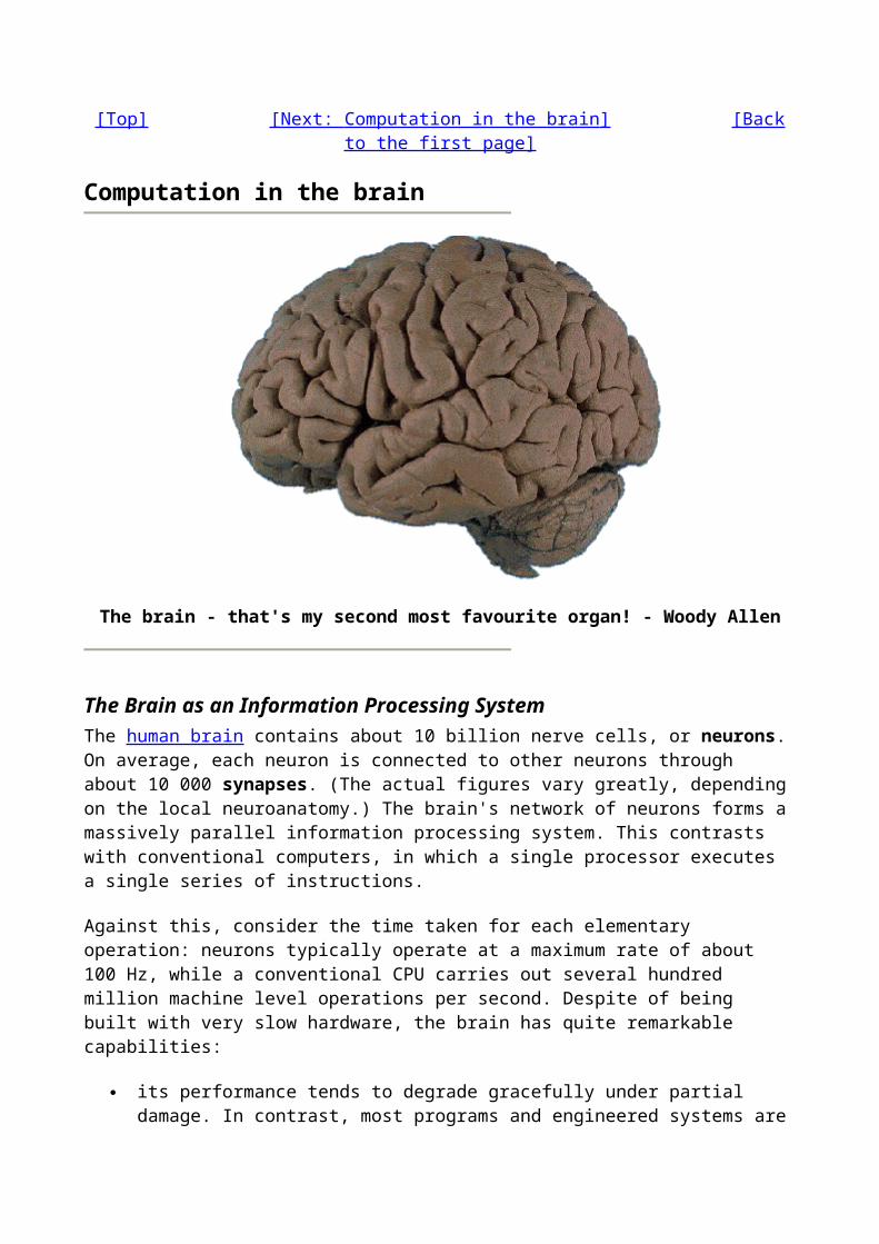
Computation in the brain

The brain - that's my second most favourite organ! - Woody Allen

The Brain as an Information Processing SystemThe human brain contains about 10 billion nerve cells, or neurons. On average, each neuron is connected to other neurons through about 10 000 synapses. (The actual figures vary greatly, depending on the local neuroanatomy.) The brain's network of neurons forms a massively parallel information processing system. This contrasts with conventional computers, in which a single processor executes a single series of instructions.

Against this, consider the time taken for each elementary operation: neurons typically operate at a maximum rate of about 100 Hz, while a conventional CPU carries out several hundred million machine level operations per second. Despite of being built with very slow hardware, the brain has quite remarkable capabilities:

its performance tends to degrade gracefully under partial damage. In contrast, most programs and engineered systems are brittle: if you remove some arbitrary parts, very likely the whole will cease to function.

it can learn (reorganize itself) from experience. this means that partial recovery from damage is possible if healthy units can learn to take

over the functions previously carried out by the damaged areas. it performs massively parallel computations extremely efficiently. For example, complex

visual perception occurs within less than 100 ms, that is, 10 processing steps! it supports our intelligence and self-awareness. (Nobody knows yet how this occurs.)

proces

elemen

energy

proces

style of co

fault t

learns

intellig

sing elements

t size

use

sing speed

mputation

olerant

ent, conscious

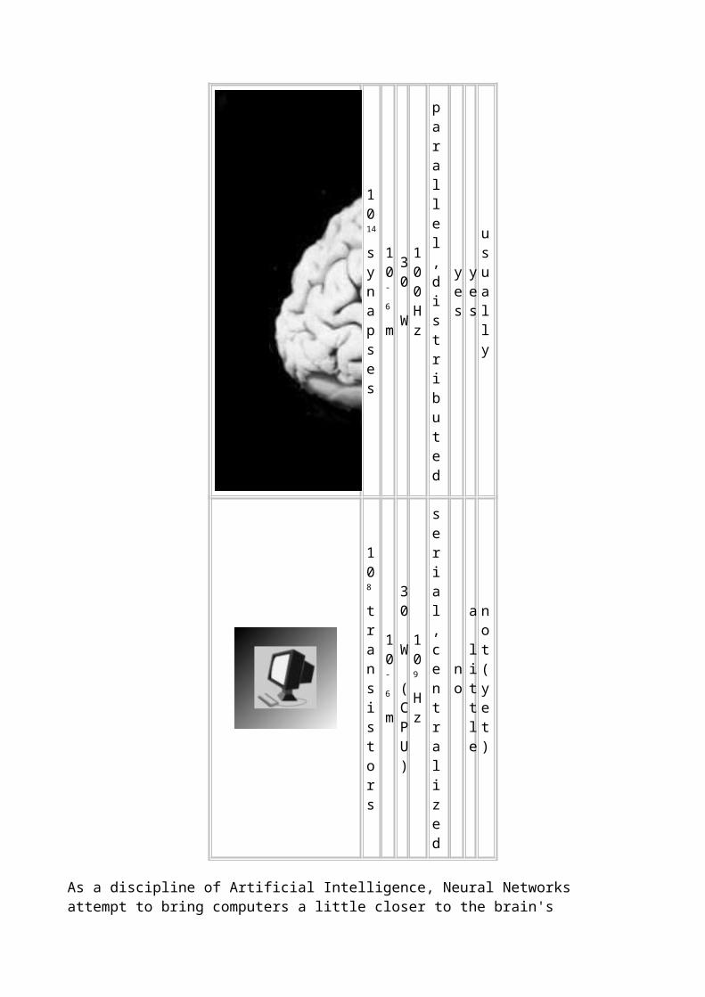
1014

synapses

10-

6

m

30 W

100 Hz

parallel, distributed

yes

yes

usually

108 transistors

10-

6

m

30 W (CPU)

109 Hz

serial, centralized

no

a little

not (yet)

As a discipline of Artificial Intelligence, Neural Networks attempt to bring computers a little closer to the brain's capabilities by imitating certain aspects of information processing in the brain, in a highly simplified way.

Neural Networks in the Brain

The brain is not homogeneous. At the largest anatomical scale, we distinguish cortex, midbrain, brainstem, and cerebellum. Each of these can be hierarchically subdivided into many regions, and areas within each region, either according to the anatomical structure of the neural networks within it, or according to the function performed by them.

The overall pattern of projections (bundles of neural connections) between areas is extremely complex, and only partially known. The best mapped (and largest) system in the human brain is the visual system, where the first 10 or 11 processing stages have been identified. We distinguish feedforward projections that go from earlier processing stages (near the sensory input) to later ones (near the motor output), from feedback connections that go in the opposite direction.

In addition to these long-range connections, neurons also link up with many thousands of their neighbours. In this way they form very dense, complex local networks:

Neurons and Synapses

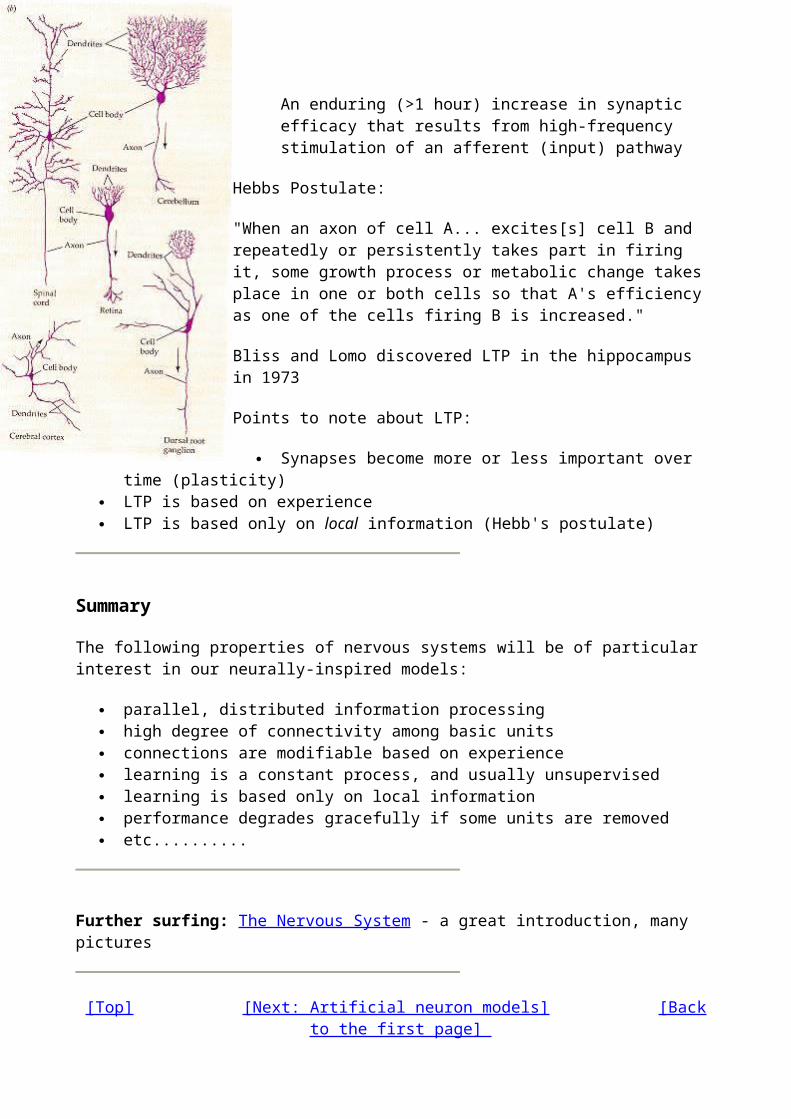
The basic computational unit in the nervous system is the nerve cell, or neuron. A neuron has:

Dendrites (inputs) Cell body Axon (output)

A neuron receives input from other neurons (typically many thousands). Inputs sum (approximately). Once input exceeds a critical level, the neuron discharges a spike - an electrical pulse that travels from the body, down the axon, to the next neuron(s) (or other receptors). This spiking event is also called depolarization, and is followed by a refractory period, during which the neuron is unable to fire.

The axon endings (Output Zone) almost touch the dendrites or cell body of the next neuron. Transmission of an electrical signal from one neuron to the next is effected by neurotransmittors, chemicals which are released from the first neuron and which bind to receptors in the second. This link is called a synapse. The extent to which the signal from one neuron is passed on to the next depends on many factors, e.g. the amount of neurotransmittor available, the number and arrangement of receptors, amount of neurotransmittor reabsorbed, etc.

Synaptic Learning

Brains learn. Of course. From what we know of neuronal structures, one way brains learn is by altering the strengths of connections between neurons, and by adding or deleting connections

between neurons. Furthermore, they learn "on-line", based on experience, and typically without the benefit of a benevolent teacher.

The efficacy of a synapse can change as a result of experience, providing both memory and learning through long-term potentiation. One way this happens is through release of more neurotransmitter. Many other changes may also be involved.

Long-term Potentiation: An enduring (>1 hour) increase in synaptic efficacy that results from high-frequency stimulation of an afferent (input) pathway

Hebbs Postulate:

"When an axon of cell A... excites[s] cell B and repeatedly or persistently takes part in firing it, some growth process or metabolic change takes place in one or both cells so that A's efficiency as one of the cells firing B is increased."

Bliss and Lomo discovered LTP in the hippocampus in 1973

Points to note about LTP:

Synapses become more or less important over time (plasticity) LTP is based on experience LTP is based only on local information (Hebb's postulate)

Summary

The following properties of nervous systems will be of particular interest in our neurally-inspired models:

parallel, distributed information processing high degree of connectivity among basic units connections are modifiable based on experience learning is a constant process, and usually unsupervised learning is based only on local information performance degrades gracefully if some units are removed etc..........

Further surfing: The Nervous System - a great introduction, many pictures

[Top] [Next: Artificial neuron models] [Back to the first page]

Artificial Neuron Models

Computational neurobiologists have constructed very elaborate computer models of neurons in order to run detailed simulations of particular circuits in the brain. As Computer Scientists, we are more interested in the general properties of neural networks, independent of how they are actually "implemented" in the brain. This means that we can use much simpler, abstract "neurons", which (hopefully) capture the essence of neural computation even if they leave out much of the details of how biological neurons work.

People have implemented model neurons in hardware as electronic circuits, often integrated on VLSI chips. Remember though that computers run much faster than brains - we can therefore run fairly large networks of simple model neurons as software simulations in reasonable time. This has obvious advantages over having to use special "neural" computer hardware.

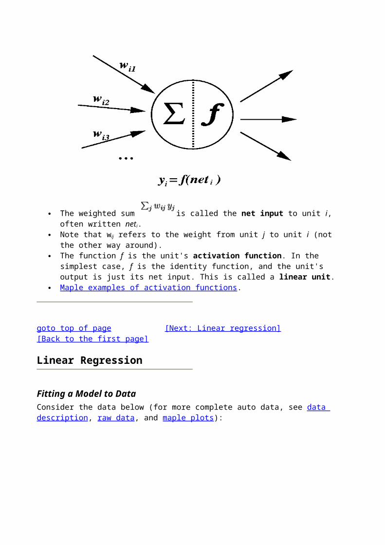
A Simple Artificial Neuron

Our basic computational element (model neuron) is often called a node or unit. It receives input from some other units, or perhaps from an external source. Each input has an associated weight w, which can be modified so as to model synaptic learning. The unit computes some function f of the weighted sum of its inputs:

Its output, in turn, can serve as input to other units.

The weighted sum is called the net input to unit i, often written neti. Note that wij refers to the weight from unit j to unit i (not the other way around).

The function f is the unit's activation function. In the simplest case, f is the identity function, and the unit's output is just its net input. This is called a linear unit.

Maple examples of activation functions .

goto top of page [Next: Linear regression] [Back to the first page]

Linear Regression

Fitting a Model to DataConsider the data below (for more complete auto data, see data description, raw data, and maple plots):

     (Fig. 1)

Each dot in the figure provides information about the weight (x-axis, units: U.S. pounds) and fuel consumption (y-axis, units: miles per gallon) for one of 74 cars (data from 1979). Clearly weight and fuel consumption are linked, so that, in general, heavier cars use more fuel.

Now suppose we are given the weight of a 75th car, and asked to predict how much fuel it will use, based on the above data. Such questions can be answered by using a model - a short mathematical description - of the data (see also optical illusions). The simplest useful model here is of the form

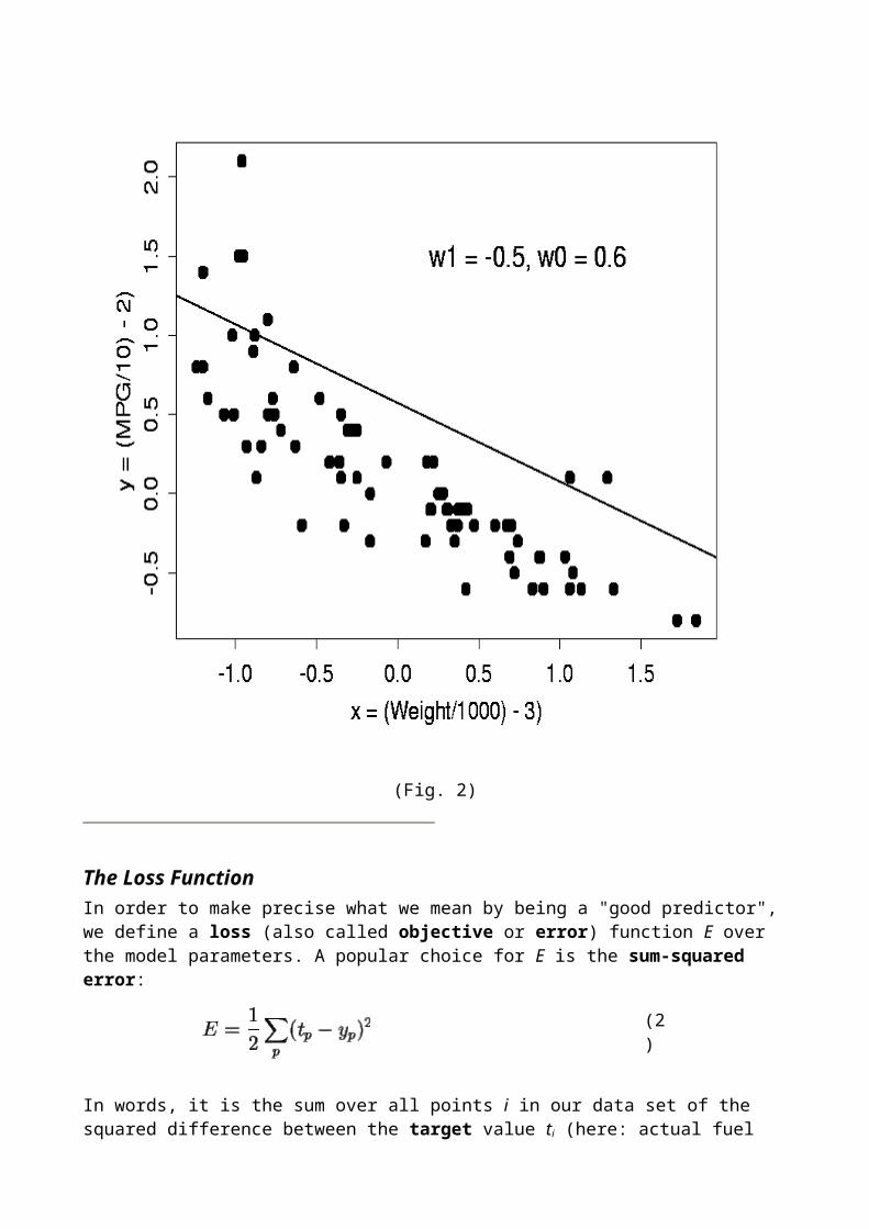
y = w1 x + w0 (1)

This is a linear model: in an xy-plot, equation 1 describes a straight line with slope w1 and intercept w0 with the y-axis, as shown in Fig. 2. (Note that we have rescaled the coordinate axes - this does not change the problem in any fundamental way.)

How do we choose the two parameters w0 and w1 of our model? Clearly, any straight line drawn somehow through the data could be used as a predictor, but some lines will do a better job than others. The line in Fig. 2 is certainly not a good model: for most cars, it will predict too much fuel consumption for a given weight.

     (Fig. 2)

The Loss FunctionIn order to make precise what we mean by being a "good predictor", we define a loss (also called objective or error) function E over the model parameters. A popular choice for E is the sum-squared error:

(2)

In words, it is the sum over all points i in our data set of the squared difference between the target value ti (here: actual fuel consumption) and the model's prediction yi, calculated from the input value xi (here: weight of the car) by equation 1. For a linear model, the sum-sqaured error is a quadratic function of the model parameters. Figure 3 shows E for a range of values of w0 and w1. Figure 4 shows the same functions as a contour plot.

     (Fig. 3)

     (Fig. 4)

Minimizing the LossThe loss function E provides us with an objective measure of predictive error for a specific choice of model parameters. We can thus restate our goal of finding the best (linear) model as finding the values for the model parameters that minimize E.

For linear models, linear regression provides a direct way to compute these optimal model parameters. (See any statistics textbook for details.) However, this analytical approach does not generalize to nonlinear models (which we will get to by the end of this lecture). Even though the solution cannot be calculated explicitly in that case, the problem can still be solved by an iterative numerical technique called gradient descent. It works as follows:

1. Choose some (random) initial values for the model parameters. 2. Calculate the gradient G of the error function with respect to each model parameter.

3. Change the model parameters so that we move a short distance in the direction of the greatest rate of decrease of the error, i.e., in the direction of -G.

4. Repeat steps 2 and 3 until G gets close to zero.

How does this work? The gradient of E gives us the direction in which the loss function at the current settting of the w has the steepest slope. In ordder to decrease E, we take a small step in the opposite direction, -G (Fig. 5).

     (Fig. 5)

By repeating this over and over, we move "downhill" in E until we reach a minimum, where G = 0, so that no further progress is possible (Fig. 6).

     (Fig. 6)

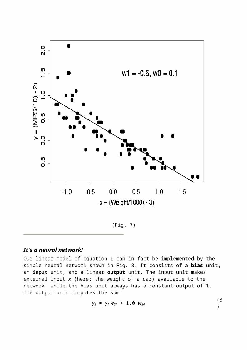
Fig. 7 shows the best linear model for our car data, found by this procedure.

     (Fig. 7)

It's a neural network!Our linear model of equation 1 can in fact be implemented by the simple neural network shown in Fig. 8. It consists of a bias unit, an input unit, and a linear output unit. The input unit makes external input x (here: the weight of a car) available to the network, while the bias unit always has a constant output of 1. The output unit computes the sum:

y2 = y1 w21 + 1.0 w20 (3) 

It is easy to see that this is equivalent to equation 1, with w21 implementing the slope of the straight line, and w20 its intercept with the y-axis.

    (Fig. 8)

[Goto top of page] [Next: Linear neural networks] [Back to the first page]

Linear Neural Networks

Multiple regression

Our car example showed how we could discover an optimal linear function for predicting one variable (fuel consumption) from one other (weight). Suppose now that we are also given one or more additional variables which could be useful as predictors. Our simple neural network model can easily be extended to this case by adding more input units (Fig. 1).

Similarly, we may want to predict more than one variable from the data that we're given. This can easily be accommodated by adding more output units (Fig. 2). The loss function for a network with multiple outputs is obtained simply by adding the loss for each output unit together. The network now has a typical layered structure: a layer of input units (and the bias), connected by a layer of weights to a layer of output units.

(Fig. 1) (Fig. 2)

Computing the gradient

In order to train neural networks such as the ones shown above by gradient descent, we need to be able to compute the gradient G of the loss function with respect to each weight wij of the network. It tells us how a small change in that weight will affect the overall error E. We begin by splitting the loss function into separate terms for each point p in the training data:

(1)

where o ranges over the output units of the network. (Note that we use the superscript p to denote the training point - this is not an exponentiation!) Since differentiation and summation are interchangeable, we can likewise split the gradient into separate components for each training point:

(2)

In what follows, we describe the computation of the gradient for a single data point, omitting the superscript p in order to make the notation easier to follow.

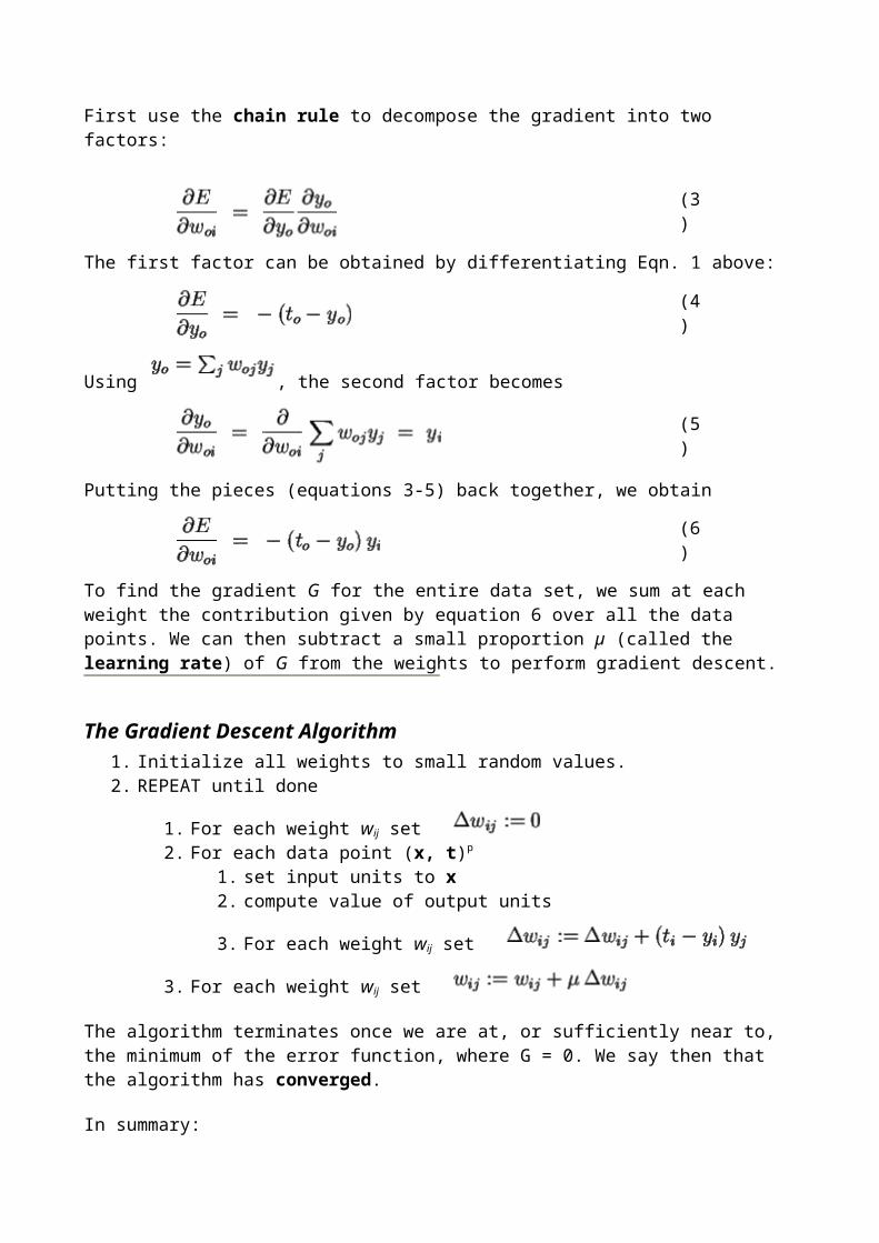
First use the chain rule to decompose the gradient into two factors:

(3)

The first factor can be obtained by differentiating Eqn. 1 above:

(4)

Using , the second factor becomes

(5)

Putting the pieces (equations 3-5) back together, we obtain

(6)

To find the gradient G for the entire data set, we sum at each weight the contribution given by equation 6 over all the data points. We can then subtract a small proportion µ (called the learning rate) of G from the weights to perform gradient descent.

The Gradient Descent Algorithm1. Initialize all weights to small random values. 2. REPEAT until done

1. For each weight wij set   2. For each data point (x, t)p

1. set input units to x 2. compute value of output units

3. For each weight wij set  

3. For each weight wij set  

The algorithm terminates once we are at, or sufficiently near to, the minimum of the error function, where G = 0. We say then that the algorithm has converged.

In summary:

general case  linear network

Training data  (x,t) (x,t)

Model parameters  w w

Model  y = g(w,x)

Error function  E(y,t)

Gradient with respect to wij

- (ti - yi) yj

Weight update rule 

The Learning Rate

An important consideration is the learning rate µ, which determines by how much we change the weights w at each step. If µ is too small, the algorithm will take a long time to converge (Fig. 3).

    (Fig. 3)Conversely, if µ is too large, we may end up bouncing around the error surface out of control - the algorithm diverges (Fig. 4). This usually ends with an overflow error in the computer's floating-point arithmetic.

    (Fig. 4)

Batch vs. Online Learning

Above we have accumulated the gradient contributions for all data points in the training set before updating the weights. This method is often referred to as batch learning. An alternative approach is online learning, where the weights are updated immediately after seeing each data point. Since the gradient for a single data point can be considered a noisy approximation to the overall gradient G (Fig. 5), this is also called stochastic (noisy) gradient descent.

    (Fig. 5)Online learning has a number of advantages:

it is often much faster, especially when the training set is redundant (contains many similar data points),

it can be used when there is no fixed training set (new data keeps coming in), it is better at tracking nonstationary environments (where the best model gradually changes

over time), the noise in the gradient can help to escape from local minima (which are a problem for

gradient descent in nonlinear models).

These advantages are, however, bought at a price: many powerful optimization techniques (such as: conjugate and second-order gradient methods, support vector machines, Bayesian methods, etc.) - which we will not talk about in this course! - are batch methods that cannot be used online. (Of course this also means that in order to implement batch learning really well, one has to learn an awful lot about these rather complicated methods!)

A compromise between batch and online learning is the use of "mini-batches": the weights are updated after every n data points, where n is greater than 1 but smaller than the training set size.

In order to keep things simple, we will focus very much on online learning, where plain gradient descent is among the best available techniques. Online learning is also highly suitable for implementing things such as reactive control strategies in adapative agents, and should thus fit in well with the rest of your course.

goto top of page [Next: Multi-layer networks] [Back to the first page]

Multi-layer networks

Multi-layer networks

A nonlinear problem

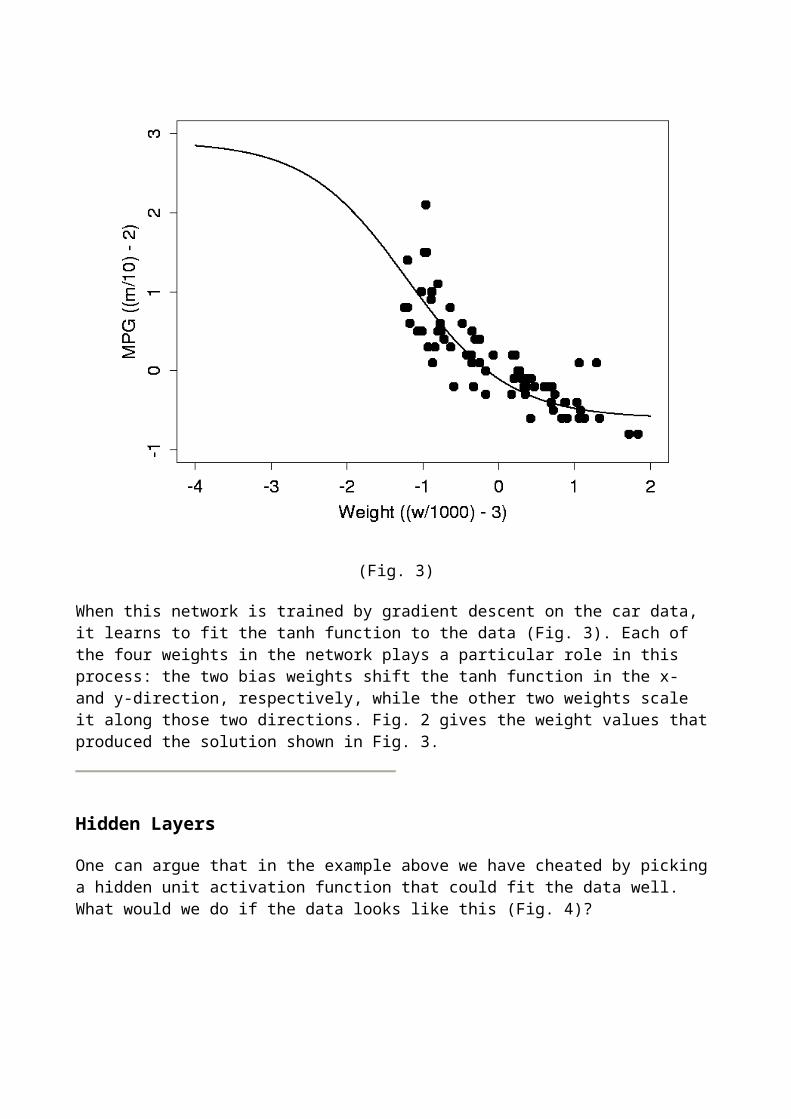
Consider again the best linear fit we found for the car data. Notice that the data points are not evenly distributed around the line: for low weights, we see more miles per gallon than our model predicts. In fact, it looks as if a simple curve might fit these data better than the straight line. We can enable our neural network to do such curve fitting by giving it an additional node which has a suitably curved (nonlinear) activation function. A useful function for this purpose is the S-shaped hyperbolic tangent (tanh) function (Fig. 1).

(Fig. 1) (Fig. 2)

FIg. 2 shows our new network: an extra node (unit 2) with tanh activation function has been inserted between input and output. Since such a node is "hidden" inside the network, it is commonly called a hidden unit. Note that the hidden unit also has a weight from the bias unit. In general, all non-input neural network units have such a bias weight. For simplicity, the bias unit and weights are usually omitted from neural network diagrams - unless it's explicitly stated otherwise, you should always assume that they are there.

  (Fig. 3)

When this network is trained by gradient descent on the car data, it learns to fit the tanh function to the data (Fig. 3). Each of the four weights in the network plays a particular role in this process: the two bias weights shift the tanh function in the x- and y-direction, respectively, while the other two weights scale it along those two directions. Fig. 2 gives the weight values that produced the solution shown in Fig. 3.

Hidden Layers

One can argue that in the example above we have cheated by picking a hidden unit activation function that could fit the data well. What would we do if the data looks like this (Fig. 4)?

  (Fig. 4)

(Relative concentration of NO and NO2 in exhaust fumes as a function of the richness of the ethanol/air mixture burned in a car engine.)

Obviously the tanh function can't fit this data at all. We could cook up a special activation function for each data set we encounter, but that would defeat our purpose of learning to model the data. We would like to have a general, non-linear function approximation method which would allow us to fit any given data set, no matter how it looks like.

  (Fig. 5)

Fortunately there is a very simple solution: add more hidden units! In fact, a network with just two hidden units using the tanh function (Fig. 5) can fit the dat in Fig. 4 quite well - can you see how? The fit can be further improved by adding yet more units to the hidden layer. Note, however, that having too large a hidden layer - or too many hidden layers - can degrade the network's performance (more on this later). In general, one shouldn't use more hidden units than necessary to solve a given problem. (One way to ensure this is to start training with a very small network. If gradient descent fails to find a satisfactory solution, grow the network by adding a hidden unit, and repeat.)

Theoretical results indicate that given enough hidden units, a network like the one in Fig. 5 can approximate any reasonable function to any required degree of accuracy. In other words, any

function can be expressed as a linear combination of tanh functions: tanh is a universal basis function. Many functions form a universal basis; the two classes of activation functions commonly used in neural networks are the sigmoidal (S-shaped) basis functions (to which tanh belongs), and the radial basis functions.

[Top] [Next: Backpropagation] [Back to the first page]

A nonlinear problem

Consider again the best linear fit we found for the car data. Notice that the data points are not evenly distributed around the line: for low weights, we see more miles per gallon than our model predicts. In fact, it looks as if a simple curve might fit these data better than the straight line. We can enable our neural network to do such curve fitting by giving it an additional node which has a suitably curved (nonlinear) activation function. A useful function for this purpose is the S-shaped hyperbolic tangent (tanh) function (Fig. 1).

(Fig. 1) (Fig. 2)

FIg. 2 shows our new network: an extra node (unit 2) with tanh activation function has been inserted between input and output. Since such a node is "hidden" inside the network, it is commonly called a hidden unit. Note that the hidden unit also has a weight from the bias unit. In general, all non-input neural network units have such a bias weight. For simplicity, the bias unit and weights are usually omitted from neural network diagrams - unless it's explicitly stated otherwise, you should always assume that they are there.

  (Fig. 3)

When this network is trained by gradient descent on the car data, it learns to fit the tanh function to the data (Fig. 3). Each of the four weights in the network plays a particular role in this process: the two bias weights shift the tanh function in the x- and y-direction, respectively, while the other two weights scale it along those two directions. Fig. 2 gives the weight values that produced the solution shown in Fig. 3.

Hidden Layers

One can argue that in the example above we have cheated by picking a hidden unit activation function that could fit the data well. What would we do if the data looks like this (Fig. 4)?

  (Fig. 4)

(Relative concentration of NO and NO2 in exhaust fumes as a function of the richness of the ethanol/air mixture burned in a car engine.)

Obviously the tanh function can't fit this data at all. We could cook up a special activation function for each data set we encounter, but that would defeat our purpose of learning to model the data. We would like to have a general, non-linear function approximation method which would allow us to fit any given data set, no matter how it looks like.

  (Fig. 5)

Error Backpropagation

We have already seen how to train linear networks by gradient descent. In trying to do the same for multi-layer networks we encounter a difficulty: we don't have any target values for the hidden units. This seems to be an insurmountable problem - how could we tell the hidden units just what to do?

This unsolved question was in fact the reason why neural networks fell out of favor after an initial period of high popularity in the 1950s. It took 30 years before the error backpropagation (or in short: backprop) algorithm popularized a way to train hidden units, leading to a new wave of neural network research and applications.

  (Fig. 1)

In principle, backprop provides a way to train networks with any number of hidden units arranged in any number of layers. (There are clear practical limits, which we will discuss later.) In fact, the network does not have to be organized in layers - any pattern of connectivity that permits a partial ordering of the nodes from input to output is allowed. In other words, there must be a way to order the units such that all connections go from "earlier" (closer to the input) to "later" ones (closer to the output). This is equivalent to stating that their connection pattern must not contain any cycles. Networks that respect this constraint are called feedforward networks; their connection pattern forms a directed acyclic graph or dag.

The Algorithm

We want to train a multi-layer feedforward network by gradient descent to approximate an unknown function, based on some training data consisting of pairs (x,t). The vector x represents a pattern of input to the network, and the vector t the corresponding target (desired output). As we have seen before, the overall gradient with respect to the entire training set is just the sum of the gradients for each pattern; in what follows we will therefore describe how to compute the gradient for just a single training pattern. As before, we will number the units, and denote the weight from unit j to unit i by wij.

1. Definitions:

o the error signal for unit j:

o the (negative) gradient for weight wij:  

o the set of nodes anterior to unit i:  

o the set of nodes posterior to unit j:  2. The gradient. As we did for linear networks before, we expand the gradient into two factors

by use of the chain rule:

The first factor is the error of unit i. The second is

Putting the two together, we get

.

To compute this gradient, we thus need to know the activity and the error for all relevant nodes in the network.

3. Forward activaction. The activity of the input units is determined by the network's external input x. For all other units, the activity is propagated forward:

Note that before the activity of unit i can be calculated, the activity of all its anterior nodes (forming the set Ai) must be known. Since feedforward networks do not contain cycles, there is an ordering of nodes from input to output that respects this condition.

4. Calculating output error. Assuming that we are using the sum-squared loss

the error for output unit o is simply

5. Error backpropagation. For hidden units, we must propagate the error back from the output nodes (hence the name of the algorithm). Again using the chain rule, we can expand the error of a hidden unit in terms of its posterior nodes:

Of the three factors inside the sum, the first is just the error of node i. The second is

while the third is the derivative of node j's activation function:

For hidden units h that use the tanh activation function, we can make use of the special identitytanh(u)' = 1 - tanh(u)2, giving us

Putting all the pieces together we get

Note that in order to calculate the error for unit j, we must first know the error of all its posterior nodes (forming the set Pj). Again, as long as there are no cycles in the network, there is an ordering of nodes from the output back to the input that respects this condition. For example, we can simply use the reverse of the order in which activity was propagated forward.

Matrix Form

For layered feedforward networks that are fully connected - that is, each node in a given layer connects to every node in the next layer - it is often more convenient to write the backprop algorithm in matrix notation rather than using more general graph form given above. In this notation, the biases weights, net inputs, activations, and error signals for all units in a layer are combined into vectors, while all the non-bias weights from one layer to the next form a matrix W. Layers are numbered from 0 (the input layer) to L (the output layer). The backprop algorithm then looks as follows:

1. Initialize the input layer:

2. Propagate activity forward: for l = 1, 2, ..., L,

where bl is the vector of bias weights.

3. Calculate the error in the output layer:

4. Backpropagate the error: for l = L-1, L-2, ..., 1,

where T is the matrix transposition operator.

5. Update the weights and biases:

You can see that this notation is significantly more compact than the graph form, even though it describes exactly the same sequence of operations.

[Top] [Next: A first example] [Back to the first page]

Backpropagation of error: an example

We will now show an example of a backprop network as it learns to model the highly nonlinear data we encountered before.

The left hand panel shows the data to be modeled. The right hand panel shows a network with two hidden units, each with a tanh nonlinear activation function. The output unit computes a linear combination of the two functions

(1)

Where

(2)

and

(3)

To begin with, we set the weights, a..g, to random initial values in the range [-1,1]. Each hidden unit is thus computing a random tanh function. The next figure shows the initial two activation functions and the output of the network, which is their sum plus a negative constant. (If you have difficulty making out the line types, the top two curves are the tanh functions, the one at the bottom is the network output).

We now train the network (learning rate 0.3), updating the weights after each pattern (online learning). After we have been through the entire dataset 10 times (10 training epochs), the functions computed look like this (the output is the middle curve):

After 20 epochs, we have (output is the humpbacked curve):

and after 27 epochs we have a pretty good fit to the data:

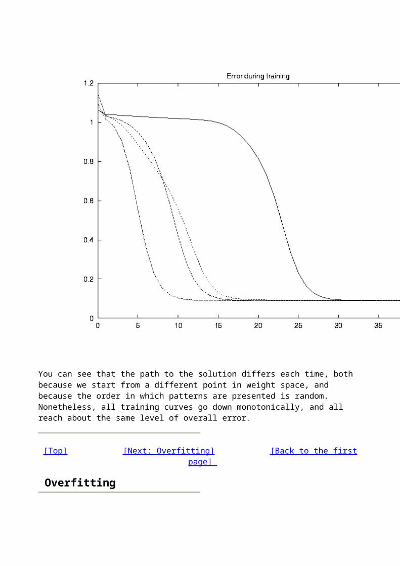
As the activation functions are stretched, scaled and shifted by the changing weights, we hope that the error of the model is dropping. In the next figure we plot the total sum squared error over all 88 patterns of the data as a function of training epoch. Four training runs are shown, with different weight initialization each time:

You can see that the path to the solution differs each time, both because we start from a different point in weight space, and because the order in which patterns are presented is random. Nonetheless, all training curves go down monotonically, and all reach about the same level of overall error.

[Top] [Next: Overfitting] [Back to the first page]

Overfitting

In the previous example we used a network with two hidden units. Just by looking at the data, it was possible to guess that two tanh functions would do a pretty good job of fitting the data. In general, however, we may not know how many hidden units, or equivalently, how many weights, we will need to produce a reasonable approximation to the data. Furthermore, we usually seek a model of the data which will give us, on average, the best possible predictions for novel data. This goal can

conflict with the simpler task of modelling a specific training set well. In this section we will look at some techniques for preventing our model becoming too powerful (overfitting). In the next, we address the related question of selecting an appropriate architecture with just the right amount of trainable parameters.

Bias-Variance trade-offConsider the two fitted functions below. The data points (circles) have all been generated from a smooth function, h(x), with some added noise. Obviously, we want to end up with a model which approximates h(x), given a specific set of data y(x) generated as:

(1)

In the left hand panel we try to fit the points using a function g(x) which has too few parameters: a straight line. The model has the virtue of being simple; there are only two free parameters. However, it does not do a good job of fitting the data, and would not do well in predicting new data points. We say that the simpler model has a high bias.

The right hand panel shows a model which has been fitted using too many free parameters. It does an excellent job of fitting the data points, as the error at the data points is close to zero. However it would not do a good job of predicting h(x) for new values of x. We say that the model has a high variance. The model does not reflect the structure which we expect to be present in any data set generated by equation (1) above.

Clearly what we want is something in between: a model which is powerful enough to represent the underlying structure of the data (h(x)), but not so powerful that it faithfully models the noise associated with this particular data sample.

The bias-variance trade-off is most likely to become a problem if we have relatively few data points. In the opposite case, where we have essentially an infinite number of data points (as in continuous online learning), we are not usually in danger of overfitting the data, as the noise associated with any single data point plays a vanishingly small role in our overall fit. The following techniques therefore apply to situations in which we have a finite data set, and, typically, where we wish to train in batch mode.

Preventing overfitting

Early stopping

One of the simplest and most widely used means of avoiding overfitting is to divide the data into two sets: a training set and a validation set. We train using only the training data. Every now and then, however, we stop training, and test network performance on the independent validation set. No weight updates are made during this test! As the validation data is independent of the training data, network performance is a good measure of generalization, and as long as the network is learning the underlying structure of the data (h(x) above), performance on the validation set will improve with training. Once the network stops learning things which are expected to be true of any data sample and learns things which are true only of this sample (epsilon in Eqn 1 above), performance on the validation set will stop improving, and will typically get worse. Schematic learning curves showing error on the training and validation sets are shown below. To avoid overfitting, we simply stop training at time t, where performance on the validation set is optimal.

One detail of note when using early stopping: if we wish to test the trained network on a set of independent data to measure its ability to generalize, we need a third, independent, test set. This is because we used the validation set to decide when to stop training, and thus our trained network is no longer entirely independent of the validation set. The requirements of independent training, validation and test sets means that early stopping can only be used in a data-rich situation.

Weight decay

The over-fitted function above shows a high degree of curvature, while the linear function is maximally smooth. Regularization refers to a set of techniques which help to ensure that the function computed by the network is no more curved than necessary. This is achieved by adding a penalty to the error function, giving:

(2)

One possible form of the regularizer comes from the informal observation that an over-fitted mapping with regions of large curvature requires large weights. We thus penalize large weights by choosing

(3)

Using this modified error function, the weights are now updated as

(4)

where the right hand term causes the weight to decrease as a function of its own size. In the absence of any input, all weights will tend to decrease exponentially, hence the term "weight decay".

Training with noise

A final method which can often help to reduce the importance of the specific noise characteristics associated with a particular data sample is to add an extra small amount of noise (a small random value with mean value of zero) to each input. Each time a specific input pattern x is presented, we

add a different random number, and use instead.

At first, this may seem a rather odd thing to do: to deliberately corrupt ones own data. However, perhaps you can see that it will now be difficult for the network to approximate any specific data point too closely. In practice, training with added noise has indeed been shown to reduce overfitting and thus improve generalization in some situations.

If we have a finite training set, another way of introducing noise into the training process is to use online training, that is, updating weights after every pattern presentation, and to randomly reorder the patterns at the end of each training epoch. In this manner, each weight update is based on a noisy estimate of the true gradient.

[Top] [Next: Growing and pruning networks] [Back to the first page]

Growing and Pruning Networks

The neural network modeler is faced with a huge array of models and training regimes from which to select. This course can only serve to introduce you to the most common and general models. However, even after deciding, for example, to train a simple feed forward network, using some specific form of gradient descent, with tanh nodes in a single hidden layer, an important question to be addressed is remains: how big a network should we choose? How many hidden units, or, relatedly, how many weights?

By way of an example, the nonlinear data which formed our first example can be fitted very well using 40 tanh functions. Learning with 40 hidden units is considerably harder than learning with 2, and takes significantly longer. The resulting fit is no better (as measured by the sum squared error) than the 2-unit model.

The most usual answer is not necessarily the best: we guess an appropriate number (as we did above).

Another common solution is to try out several network sizes, and select the most promising. Neither of these methods is very principled.

Two more rigorous classes of methods are available, however. We can either start with a network which we know to be too small, and iteratively add units and weights, or we can train an oversized network and remove units/weights from the final network. We will look briefly at each of these approaches.

Growing networks

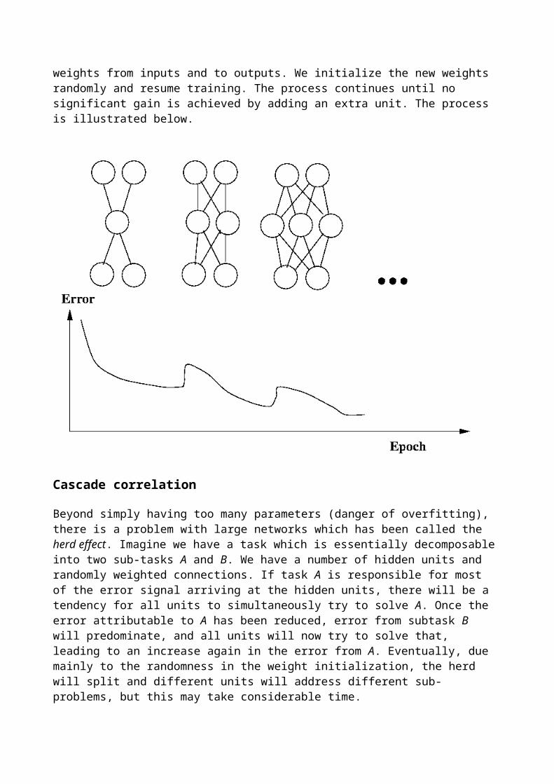
The simplest form of network growing algorithm starts with a small network, say one with only a single hidden unit. The network is trained until the improvement in the error over one epoch falls below some threshold. We then add an additional hidden unit, with weights from inputs and to outputs. We initialize the new weights randomly and resume training. The process continues until no significant gain is achieved by adding an extra unit. The process is illustrated below.

Cascade correlation

Beyond simply having too many parameters (danger of overfitting), there is a problem with large networks which has been called the herd effect. Imagine we have a task which is essentially decomposable into two sub-tasks A and B. We have a number of hidden units and randomly weighted connections. If task A is responsible for most of the error signal arriving at the hidden units, there will be a tendency for all units to simultaneously try to solve A. Once the error attributable to A has been reduced, error from subtask B will predominate, and all units will now try to solve that, leading to an increase again in the error from A. Eventually, due mainly to the randomness in the weight initialization, the herd will split and different units will address different sub-problems, but this may take considerable time.

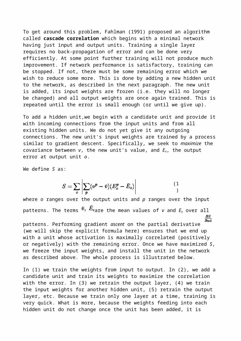
To get around this problem, Fahlman (1991) proposed an algorithm called cascade correlation which begins with a minimal network having just input and output units. Training a single layer requires no back-propagation of error and can be done very efficiently. At some point further training will not produce much improvement. If network performance is satisfactory, training can be stopped. If not, there must be some remaining error which we wish to reduce some more. This is done by adding a new hidden unit to the network, as described in the next paragraph. The new unit is added, its input weights are frozen (i.e. they will no longer be changed) and all output weights are once again trained. This is repeated until the error is small enough (or until we give up).

To add a hidden unit,we begin with a candidate unit and provide it with incoming connections from the input units and from all existing hidden units. We do not yet give it any outgoing connections. The new unit's input weights are trained by a process similar to gradient descent. Specifically, we

seek to maximize the covariance between v, the new unit's value, and Eo, the output error at output unit o.

We define S as:

(1)

where o ranges over the output units and p ranges over the input patterns. The terms are the

mean values of v and Eo over all patterns. Performing gradient ascent on the partial derivative (we will skip the explicit formula here) ensures that we end up with a unit whose activation is maximally correlated (positively or negatively) with the remaining error. Once we have maximized S, we freeze the input weights, and install the unit in the network as described above. The whole process is illustrated below.

In (1) we train the weights from input to output. In (2), we add a candidate unit and train its weights to maximize the correlation with the error. In (3) we retrain the output layer, (4) we train the input weights for another hidden unit, (5) retrain the output layer, etc. Because we train only one layer at a time, training is very quick. What is more, because the weights feeding into each hidden unit do not change once the unit has been added, it is possible to record and store the activations of the hidden units for each pattern, and reuse these values without recomputation in later epochs.

Pruning networks

An alternative approach to growing networks is to start with a relatively large network and then remove weights so as to arrive at an optimal network architecture. The usual procedure is as follows:

1. Train a large, densely connected, network with a standard training algorithm 2. Examine the trained network to assess the relative importance of the weights 3. Remove the least important weight(s) 4. retrain the pruned network 5. Repeat steps 2-4 until satisfied

Deciding which are the least important weights is a difficult issue for which several heuristic approaches are possible. We can estimate the amount by which the error function E changes for a small change in each weight. The computational form for this estimate would take us a little too far here. Various forms of this technique have been called optimal brain damage, and optimal brain surgeon.

[Top] [Next: Preconditioning the network] [Back to the first page]

Preconditioning the Network

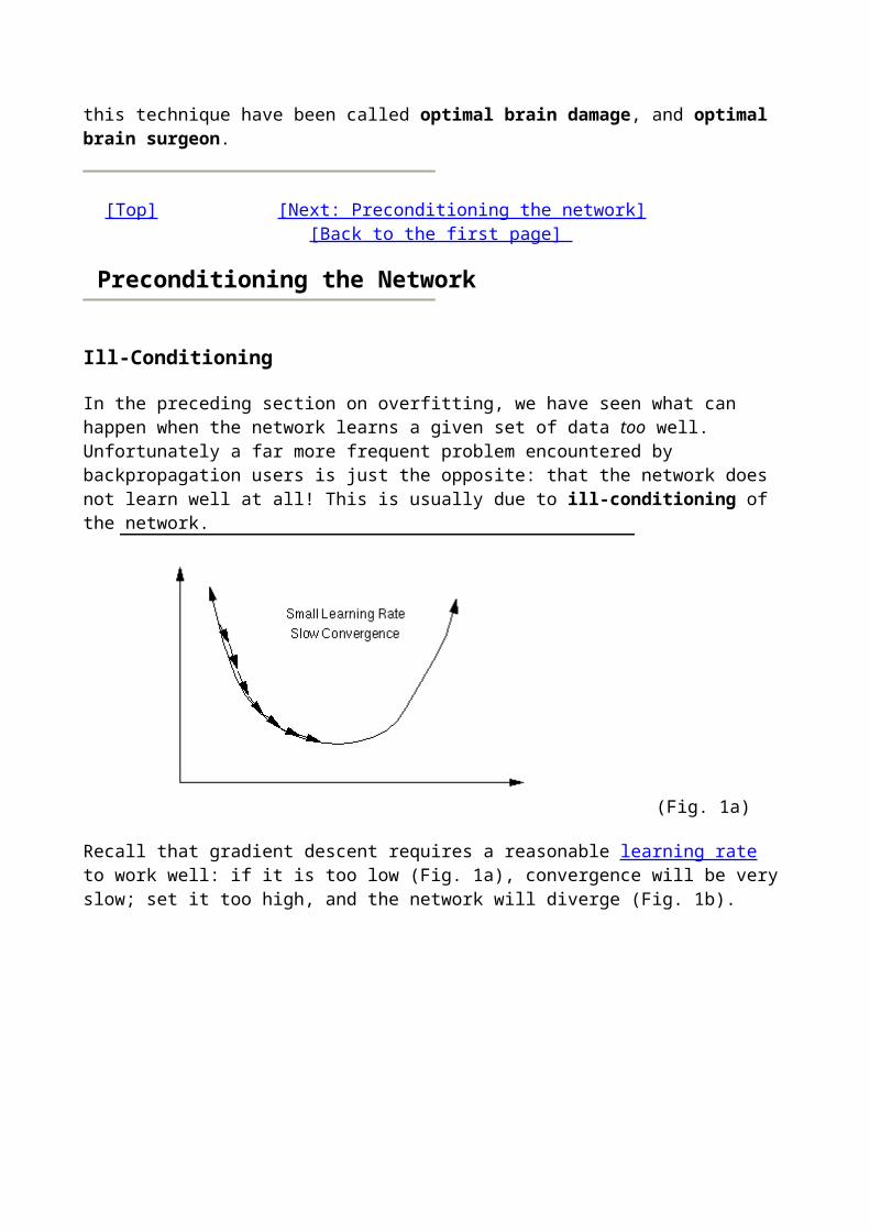
Ill-Conditioning

In the preceding section on overfitting, we have seen what can happen when the network learns a given set of data too well. Unfortunately a far more frequent problem encountered by backpropagation users is just the opposite: that the network does not learn well at all! This is usually due to ill-conditioning of the network.

  (Fig. 1a)

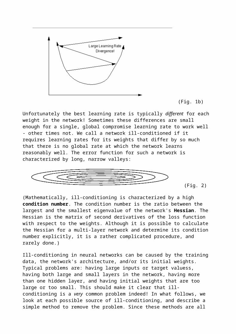
Recall that gradient descent requires a reasonable learning rate to work well: if it is too low (Fig. 1a), convergence will be very slow; set it too high, and the network will diverge (Fig. 1b).

  (Fig. 1b)

Unfortunately the best learning rate is typically different for each weight in the network! Sometimes these differences are small enough for a single, global compromise learning rate to work well - other times not. We call a network ill-conditioned if it requires learning rates for its weights that differ by so much that there is no global rate at which the network learns reasonably well. The error function for such a network is characterized by long, narrow valleys:

  (Fig. 2)

(Mathematically, ill-conditioning is characterized by a high condition number. The condition number is the ratio between the largest and the smallest eigenvalue of the network's Hessian. The Hessian is the matrix of second derivatives of the loss function with respect to the weights. Although it is possible to calculate the Hessian for a multi-layer network and determine its condition number explicitly, it is a rather complicated procedure, and rarely done.)

Ill-conditioning in neural networks can be caused by the training data, the network's architecture, and/or its initial weights. Typical problems are: having large inputs or target valuess, having both large and small layers in the network, having more than one hidden layer, and having initial weights that are too large or too small. This should make it clear that ill-conditioning is a very common problem indeed! In what follows, we look at each possible source of ill-conditioning, and describe a simple method to remove the problem. Since these methods are all used before training of the network begins, we refer to them as preconditioning techniques.

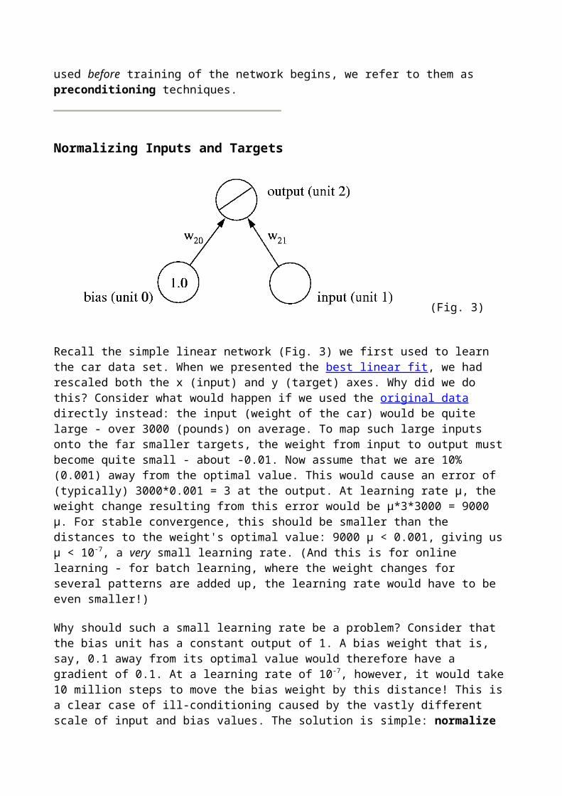
Normalizing Inputs and Targets

  (Fig. 3)

Recall the simple linear network (Fig. 3) we first used to learn the car data set. When we presented the best linear fit, we had rescaled both the x (input) and y (target) axes. Why did we do this? Consider what would happen if we used the original data directly instead: the input (weight of the car) would be quite large - over 3000 (pounds) on average. To map such large inputs onto the far smaller targets, the weight from input to output must become quite small - about -0.01. Now assume that we are 10% (0.001) away from the optimal value. This would cause an error of (typically) 3000*0.001 = 3 at the output. At learning rate µ, the weight change resulting from this error would be µ*3*3000 = 9000 µ. For stable convergence, this should be smaller than the distances to the weight's optimal value: 9000 µ < 0.001, giving us µ < 10-7, a very small learning rate. (And this is for online learning - for batch learning, where the weight changes for several patterns are added up, the learning rate would have to be even smaller!)

Why should such a small learning rate be a problem? Consider that the bias unit has a constant output of 1. A bias weight that is, say, 0.1 away from its optimal value would therefore have a gradient of 0.1. At a learning rate of 10-7, however, it would take 10 million steps to move the bias weight by this distance! This is a clear case of ill-conditioning caused by the vastly different scale of input and bias values. The solution is simple: normalize the input, so that it has an average of zero and a standard deviation of one. Normalization is a two-step process:

To normalize a variable, first

1. (centering) subtract its average, then

2. (scaling) divide by its standard deviation.

Note that for our purposes it is not really necessary to calculate the mean and standard deviation of each input exactly - approximate values are perfectly sufficient. (In the case of the car data, the "mean" of 3000 and "standard deviation" of 1000 were simply guessed after looking at the data plot.) This means that in situations where the training data is not known in advance, estimates based on either prior knowledge or a small sample of the data are usually good enough. If the data is a time series x(t), you may also want to consider using the first differences x(t) - x(t-1) as network inputs instead; they have zero mean as long as x(t) is stationary. Whichever way you do it, remember that you should always

normalize the inputs, and normalize the targets.

To see why the target values should also be normalized, consider the network we've used to fit a sigmoid to the car data (Fig. 4). If the target values were those found in the original data, the weight from hidden to output unit would have to be 10 times larger. The error signal propagated back to the hidden unit would thus be multiplied by 17 along the way. In order to compensate for this, the global learning rate would have to be lowered correspondingly, slowing down the weights that go directly to the output unit. Thus while large inputs cause ill-conditioning by leading to very small weights, large targets do so by leading to very large weights.

Finally, notice that the argument for normalizing the inputs can also be applied to the hidden units (which after all look like inputs to their posterior nodes). Ideally, we would like hidden unit activations as well to have a mean of zero and a standard deviation of one. Since the weights into hidden units keep changing during training, however, it would be rather hard to predict their mean and standard deviation accurately! Fortunately we can rely on our tanh activation function to keep things reasonably well-conditioned: its range from -1 to +1 implies that the standard deviation cannot exceed 1, while its symmetry about zero means that the mean will typically be relatively small. Furthermore, its maximum derivative is also 1, so that backpropagated errors will be neither magnified nor attenuated more than necessary.

Note: For historic reasons, many people use the logistic sigmoid   f(u) = 1/(1 + e-u)   as activation function for hidden units. This function is closely related to tanh (in fact, f(u) = tanh(u/2)/2 + 0.5) but has a smaller, asymmetric range (from 0 to 1), and a maximum derivative of 0.25. We will later encounter a legitimate use for this function, but as activation function for hidden units it tends to orsen the network's conditioning. Thus

do not use the logistic sigmoid   f(u) = 1/(1 + e-u)   as activation function for hidden units.

Use tanh instead: your network will be better conditioned.

Initializing the Weights

Before training, the network weights are initialized to small random values. The random values are usually drawn from a uniform distribution over the range [-r,r]. What should r be? If the initial weights are too small, both activation and error signals will die out along their way through the network. Conversely, if they are too large, the tanh function of the hidden units will saturate - be very close to its asymptotic value of +/-1. This means that its derivative will be close to zero, blocking any backpropagated error signals from passing through the node; this is sometimes called paralysis of the node.

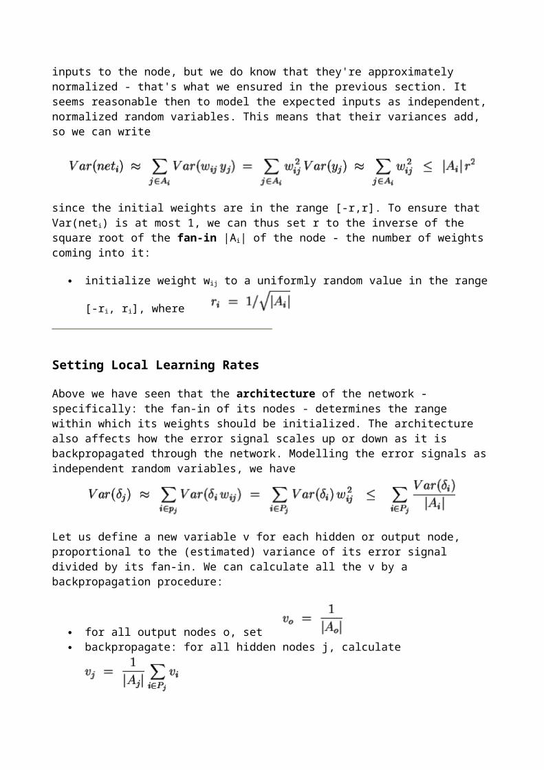
To avoid either extreme, we would initally like the hidden units' net input to be approximately normalized. We do not know the inputs to the node, but we do know that they're approximately normalized - that's what we ensured in the previous section. It seems reasonable then to model the expected inputs as independent, normalized random variables. This means that their variances add, so we can write

(Fig. 4)

since the initial weights are in the range [-r,r]. To ensure that Var(neti) is at most 1, we can thus set r to the inverse of the square root of the fan-in |Ai| of the node - the number of weights coming into it:

initialize weight wij to a uniformly random value in the range [-ri, ri], where   

Setting Local Learning Rates

Above we have seen that the architecture of the network - specifically: the fan-in of its nodes - determines the range within which its weights should be initialized. The architecture also affects how the error signal scales up or down as it is backpropagated through the network. Modelling the error signals as independent random variables, we have

Let us define a new variable v for each hidden or output node, proportional to the (estimated) variance of its error signal divided by its fan-in. We can calculate all the v by a backpropagation procedure:

for all output nodes o, set  

backpropagate: for all hidden nodes j, calculate  

Since the activations in the network are already normalized, we can expect the gradient for weight wij to scale with the square root of the corresponding error signal's variance, vi|Ai|. The resulting weight change, however, should be commensurate with the characteristic size of the weight, which is given by ri. To achieve this,

set the learning rate µi (used for all weights wij into node i) to  

If you follow all the points we have made in this section before the start of training, you should have a reasonably well-conditioned network that can be trained effectively. It remains to determine a good global learning rate µ. This must be done by trial and error; a good first guess (on the high size) would be the inverse of the square root of the batch size (by a similar argument as we have made above), or 1 for online learning. If this leads to divergence, reduce µ and try again.

[Top] [Next: Momentum and learning rate adaptation] [Back to the first page]

Momentum and Learning Rate Adaptation

Local Minima

In gradient descent we start at some point on the error function defined over the weights, and attempt to move to the global minimum of the function. In the simplified function of Fig 1a the situation is simple. Any step in a downward direction will take us closer to the global minimum. For real problems, however, error surfaces are typically complex, and may more resemble the situation shown in Fig 1b. Here there are numerous local minima, and the ball is shown trapped in one such minimum. Progress here is only possible by climbing higher before descending to the global minimum.

  (Fig. 1a)   (Fig. 1b)

We have already mentioned one way to escape a local minimum: use online learning. The noise in the stochastic error surface is likely to bounce the network out of local minima as long as they are not too severe.

MomentumAnother technique that can help the network out of local minima is the use of a momentum term. This is probably the most popular extension of the backprop algorithm; it is hard to find cases where this is not used. With momentum m, the weight update at a given time t becomes

(1)

where 0 < m < 1 is a new global parameter which must be determined by trial and error. Momentum simply adds a fraction m of the previous weight update to the current one. When the gradient keeps pointing in the same direction, this will increase the size of the steps taken towards the minimum. It is otherefore often necessary to reduce the global learning rate µ when using a lot of momentum (m

close to 1). If you combine a high learning rate with a lot of momentum, you will rush past the minimum with huge steps!

When the gradient keeps changing direction, momentum will smooth out the variations. This is particularly useful when the network is not well-conditioned. In such cases the error surface has substantially different curvature along different directions, leading to the formation of long narrow valleys. For most points on the surface, the gradient does not point towards the minimum, and successive steps of gradient descent can oscillate from one side to the other, progressing only very slowly to the minimum (Fig. 2a). Fig. 2b shows how the addition of momentum helps to speed up convergence to the minimum by damping these oscillations.

  (Fig. 2a)   (Fig. 2b)

To illustrate this effect in practice, we trained 20 networks on a simple problem (4-2-4 encoding), both with and without momentum. The mean training times (in epochs) were

momentum Training time

0 217

0.9 95

Learning Rate Adaptation

In the section on preconditioning, we have employed simple heuristics to arrive at reasonable guesses for the global and local learning rates. It is possible to refine these values significantly once training has commenced, and the network's response to the data can be observed. We will now introduce a few methods that can do so automatically by adapting the learning rates during training.

Bold Driver

A useful batch method for adapting the global learning rate µ is the bold driver algorithm. Its operation is simple: after each epoch, compare the network's loss E(t) to its previous value, E(t-1). If the error has decreased, increase µ by a small proportion (typically 1%-5%). If the error has increased by more than a tiny proportion (say, 10-10), however, undo the last weight change, and decrease µ sharply - typically by 50%. Thus bold driver will keep growing µ slowly until it finds itself taking a step that has clearly gone too far up onto the opposite slope of the error function. Since this means that the network has arrived in a tricky area of the error surface, it makes sense to reduce the step size quite drastically at this point.

Annealing

Unfortunately bold driver cannot be used in this form for online learning: the stochastic fluctuations in E(t) would hopelessly confuse the algorithm. If we keep µ fixed, however, these same fluctuations prevent the network from ever properly converging to the minimum - instead we end up randomly dancing around it. In order to actually reach the minimum, and stay there, we must anneal (gradually lower) the global learning rate. A simple, non-adaptive annealing schedule for this purpose is the search-then-converge schedule

µ(t) = µ(0)/(1 + t/T) (2)

Its name derives from the fact that it keeps µ nearly constant for the first T training patterns, allowing the network to find the general location of the minimum, before annealing it at a (very slow) pace that is known from theory to guarantee convergence to the minimum. The characteristic time T of this schedule is a new free parameter that must be determined by trial and error.

Local Rate Adaptation

If we are willing to be a little more sophisticated, we go a lot further than the above global methods. First let us define an online weight update that uses a local, time-varying learning rate for each weight:

(3)

The idea is to adapt these local learning rates by gradient descent, while simultaneously adapting the weights. At time t, we would like to change the learning rate (before changing the weight) such that the loss E(t+1) at the next time step is reduced. The gradient we need is

(4)

Ordinary gradient descent in µij, using the meta-learning rate q (a new global parameter), would give

(5)

We can already see that this would work in a similar fashion to momentum: increase the learning rate as long as the gradient keeps pointing in the same direction, but decrease it when you land on the opposite slope of the loss function.

Problem: µij might become negative! Also, the step size should be proportional to µij so that it can be adapted over several orders of magnitude. This can be achieved by performing the gradient descent on log(µij) instead:

(6)

Exponentiating this gives

(7)

where the approximation serves to avoid an expensive exp function call. The multiplier is limited below by 0.5 to guard against very small (or even negative) factors.

Problem: the gradient is noisy; the product of two of them will be even noisier - the learning rate will bounce around a lot. A popular way to reduce the stochasticity is to replace the gradient at the previous time step (t-1) by an exponential average of past gradients. The exponential average of a time series u(t) is defined as

(8)

where 0 < m < 1 is a new global parameter.

Problem: if the gradient is ill-conditioned, the product of two gradients will be even worse - the condition number is squared. We will need to normalize the step sizes in some way. A radical solution is to throw away the magnitude of the step, and just keep the sign, giving

(9)

where r = eq. This works fine for batch learning, but...

  (Fig. 3)

Problem: Nonlinear normalizers such as the sign function lead to systematic errors in stochastic gradient descent (Fig. 3): a skewed but zero-mean gradient distribution (typical for stochastic equilibrium) is mapped to a normalized distribution with non-zero mean. To avoid the problems this is casuing, we need a linear normalizer for online learning. A good method is to divide the step by

, an exponential average of the squared gradient. This gives

(10)

Problem: successive training patterns may be correlated, causing the product of stochastic gradients to behave strangely. The exponential averaging does help to get rid of short-term correlations, but it cannot deal with input that exhibits correlations across long periods of time. If you are iterating over a fixed training set, make sure you permute (shuffle) it before each iteration to destroy any correlations. This may not be possible in a true online learning situation, where training data is received one pattern at a time.

To show that all these equations actually do something useful, here is a typical set of online learning curves (in postscript) for a difficult benchmark problem, given either uncorrelated training patterns, or patterns with strong short-term or long-term correlations. In these figures "momentum" corresponds to using equation (1) above, and "s-ALAP" to equation (10). "ALAP" is like "s-ALAP" but without the exponential averaging of past gradients, while "ELK1" and "SMD" are more advanced methods (developed by one of us).

[Top] [Next: Classification] [Back to the first page]

Classification

Discriminants

Neural networks can also be used to classify data. Unlike regression problems, where the goal is to produce a particular output value for a given input, classification problems require us to label each data point as belonging to one of n classes. Neural networks can do this by learning a discriminant function which separates the classes. For example, a network with a single linear output can solve a two-class problem by learning a discriminant function which is greater than zero for one class, and less than zero for the other. Fig. 6 shows two such two-class problems, with filled dots belonging to one class, and unfilled dots to the other. In each case, a line is drawn where a discriminant function that separates the two classes is zero.

  (Fig. 6)

On the left side, a straight line can serve as a discriminant: we can place the line such that all filled dots lie on one side, and all unfilled ones lie on the other. The classes are said to be linearly separable. Such problems can be learned by neural networks without any hidden units. On the right side, a highly non-linear function is required to ensure class separation. This problem can be solved only by a neural network with hidden units.

Binomial

To use a neural network for classification, we need to construct an equivalent function approximation problem by assigning a target value for each class. For a binomial (two-class) problem we can use a network with a single output y, and binary target values: 1 for one class, and 0 for the other. We can thus interpret the network's output as an estimate of the probability that a given pattern belongs to the '1' class. To classify a new pattern after training, we then employ the maximum likelihood discriminant, y > 0.5.

A network with linear output used in this fashion, however, will expend a lot of its effort on getting the target values exactly right for its training points - when all we actually care about is the correct positioning of the discriminant. The solution is to use an activation function at the output that saturates at the two target values: such a function will be close to the target value for any net input that is sufficiently large and has the correct sign. Specifically, we use the logistic sigmoid function

Given the probabilistic interpretation, a network output of, say, 0.01 for a pattern that is actually in the '1' class is a much more serious error than, say, 0.1. Unfortunately the sum-squared loss function makes almost no distinction between these two cases. A loss function that is appropriate for dealing with probabilities is the cross-entropy error. For the two-class case, it is given by

When logistic output units and cross-entropy error are used together in backpropagation learning, the error signal for the output unit becomes just the difference between target and output:

In other words, implementing cross-entropy error for this case amounts to nothing more than omitting the f'(net) factor that the error signal would otherwise get multiplied by. This is not an accident, but indicative of a deeper mathematical connection: cross-entropy error and logistic outputs are the "correct" combination to use for binomial probabilities, just like linear outputs and sum-squared error are for scalar values.

Multinomial

If we have multiple independent binary attributes by which to classify the data, we can use a network with multiple logistic outputs and cross-entropy error. For multinomial classification problems (1-of-n, where n > 2) we use a network with n outputs, one corresponding to each class, and target values of 1 for the correct class, and 0 otherwise. Since these targets are not independent of each other, however, it is no longer appropriate to use logistic output units. The corect generalization of the logistic sigmoid to the multinomial case is the softmax activation function:

where o ranges over the n output units. The cross-entropy error for such an output layer is given by

Since all the nodes in a softmax output layer interact (the value of each node depends on the values of all the others), the derivative of the cross-entropy error is difficult to calculate. Fortunately, it again simplifies to

so we don't have to worry about it.

[Top] [Next: Non-Supervised Learning] [Back to the first page]

Non-Supervised Learning

It is possible to use neural networks to learn about data that contains neither target outputs nor class labels. There are many tricks for getting error signals in such non-supervised settings; here we'll briefly discuss a few of the most common approaches: autoassociation, time series prediction, and reinforcement learning.

Autoassociation

Autoassociation is based on a simple idea: if you have inputs but no targets, just use the inputs as targets. An autoassociator network thus tries to learn the identity function. This is only non-trivial if the hidden layer forms an information bottleneck - contains less units than the input (output) layer, so that the network must perform dimensionality reduction (a form of data compression).

A linear autoassociator trained with sum-squared error in effect performs principal component analysis (PCA), a well-known statistical technique. PCA extracts the subspace (directions) of highest variance from the data. As was the case with regression, the linear neural network offers no

direct advantage over known statistical methods, but it does suggest an interesting nonlinear generalization:

This nonlinear autoassociator includes a hidden layer in both the encoder and the decoder part of the network. Together with the linear bottleneck layer, this gives a network with at least 3 hidden layers. Such a deep network should be preconditioned if it is to learn successfully.

Time Series Prediction

When the input data x forms a temporal series, an important task is to predict the next point: the weather tomorrow, the stock market 5 minutes from now, and so on. We can (attempt to) do this with a feedforward network by using time-delay embedding: at time t, we give the network x(t), x(t-1), ... x(t-d) as input, and try to predict x(t+1) at the output. After propagating activity forward to make the prediction, we wait for the actual value of x(t+1) to come in before calculating and backpropagating the error. Like all neural network architecture parameters, the dimension d of the embedding is an important but difficult choice.

A more powerful (but also more complicated) way to model a time series is to use recurrent neural networks.

Reinforcement Learning

Sometimes we are faced with the problem of delayed reward: rather than being told the correct answer for each input pattern immediately, we may only occasionally get a positive or negative reinforcement signal to tell us whether the entire sequence of actions leading up to this was good or bad. Reinforcement learning provides ways to get a continuous error signal in such situations.

Q-learning associates an expected utility (the Q-value) with each action possible in a particular state. If at time t we are in state s(t) and decide to perform action a(t), the corresponding Q-value is updated as follows:

where r(t) is the instantaneous reward resulting from our action, s(t+1) is the state that it led to, a are all possible actions in that state, and gamma <= 1 is a discount factor that leads us to prefer instantaneous over delayed rewards.

A common way to implement Q-learning for small problems is to maintain a table of Q-values for all possible state/action pairs. For large problems, however, it is often impossible to keep such a large table in memory, let alone learn its entries in reasonable time. In such cases a neural network can provide a compact approximation of the Q-value function. Such a network takes the state s(t) as its input, and has an output ya for each possible action. To learn the Q-value Q(s(t), a(t)), it uses the right-hand side of the above Q-iteration as a target:

Note that since we require the network's outputs at time t+1 in order to calculate its error signal at time t, we must keep a one-step memory of all input and hidden node activity, as well as the most recent action. The error signal is applied only to the output corresponding to that action; all other output nodes receive no error (they are "don't cares").

TD-learning is a variation that assigns utility values to states alone rather than state/action pairs. This means that search must be used to determine the value of the best successor state. TD( ) replaces the one-step memory with an exponential average of the network's gradient; this is similar to momentum, and can help speed the transport of delayed reward signals across large temporal distances.

One of the most successful applications of neural networks is TD-Gammon, a network that used TD( ) to learn the game of backgammon from scratch, by playing only against itself. TD-Gammon is now the world's strongest backgammon program, and plays at the level of human grandmasters.

[Top] [Next: Recurrent neural networks] [Back to the first page]

Learning Time Sequences

There are many tasks that require learning a temporal sequence of events. These problems can be broken into 3 distinct types of tasks:

Sequence Recognition: Produce a particular output pattern when a specific input sequence is seen. Applications: speech recognition

Sequence Reproduction: Generate the rest of a sequence when the network sees only part of the sequence. Applications: Time series prediction (stock market, sun spots, etc)

Temporal Association: Produce a particular output sequence in response to a specific input sequence. Applications: speech generation

Some of the methods that are used include

Tapped Delay Lines (time delay networks) Context Units (e.g. Elman Nets, Jordan Nets) Back propagation through time (BPTT) Real Time Recurrent Learning (RTRL)

Tapped Delay Lines / Time Delay Neural Networks

One of the simplest ways of performing sequence recognition because conventional backpropagation algorithms can be used.

Downsides: Memory is limited by length of tapped delay line. If a large number of input units are needed then computation can be slow and many examples are needed.

A simple extension to this is to allow non-uniform sampling:

where i is the integer delay assoicated with component i. Thus if there are n input units, the memory is not limited simply the previous n timesteps.

Another extension that deals is for each "input" to really be a convolution of the original input sequence.

In the case of the delay line memories:

Other variations for c are shown graphically below:

This figure is taken from "Neural Net Architectures for Temporal Sequence Processing", by Mike Moser.

[Top] [ Next: Recurrent Networks I ] [Back to the first page]

Recurrent Networks I

Consider the following two networks:

    (Fig. 1)

The network on the left is a simple feed forward network of the kind we have already met. The right hand network has an additional connection from the hidden unit to itself. What difference could this seemingly small change to the network make?

Each time a pattern is presented, the unit computes its activation just as in a feed forward network. However its net input now contains a term which reflects the state of the network (the hidden unit activation) before the pattern was seen. When we present subsequent patterns, the hidden and output units' states will be a function of everything the network has seen so far.

The network behavior is based on its history, and so we must think of pattern presentation as it happens in time.

Network topology

Once we allow feedback connections, our network topology becomes very free: we can connect any unit to any other, even to itself. Two of our basic requirements for computing activations and errors in the network are now violated. When computing activations, we required that before computing yi, we had to know the activations of all units in the posterior set of nodes, Pi. For computing errors,

we required that before computing , we had to know the errors of all units in its anterior set of nodes, Ai.

For an arbitrary unit in a recurrent network, we now define its activation at time t as:

yi(t) = fi(neti(t-1))

At each time step, therefore, activation propagates forward through one layer of connections only. Once some level of activation is present in the network, it will continue to flow around the units, even in the absence of any new input whatsoever. We can now present the network with a time series of inputs, and require that it produce an output based on this series. These networks can be used to model many new kinds of problems, however, these nets also present us with many new difficult issues in training.

Before we address the new issues in training and operation of recurrent neural networks, let us first look at some sample tasks which have been attempted (or solved) by such networks.

Learning formal grammars

Given a set of strings S, each composed of a series of symbols, identify the strings which belong to a language L. A simple example: L = {an,bn} is the language composed of strings of any number of a's, followed by the same number of b's. Strings belonging to the language include aaabbb, ab, aaaaaabbbbbb. Strings not belonging to the language include aabbb, abb, etc. A common benchmark is the language defined by the reber grammar. Strings which belong to a language L are said to be grammatical and are ungrammatical otherwise.

Speech recognition

In some of the best speech recognition systems built so far, speech is first presented as a series of spectral slices to a recurrent network. Each output of the network represents the probability of a specific phone (speech sound, e.g. /i/, /p/, etc), given both present and recent input. The probabilities are then interpreted by a Hidden Markov Model which tries to recognize the whole utterance. Details are provided here.

Music composition

A recurrent network can be trained by presenting it with the notes of a musical score. It's task is to predict the next note. Obviously this is impossible to do perfectly, but the network learns that some notes are more likely to occur in one context than another. Training, for example, on a lot of music by J. S. Bach, we can then seed the network with a musical phrase, let it predict the next note, feed this back in as input, and repeat, generating new music. Music generated in this fashion typically sounds fairly convincing at a very local scale, i.e. within a short phrase. At a larger scale, however, the compositions wander randomly from key to key, and no global coherence arises. This is an interesting area for further work.... The original work is described here.

The Simple Recurrent Network

One way to meet these requirements is illustrated below in a network known variously as an Elman network (after Jeff Elman, the originator), or as a Simple Recurrent Network. At each time step, a copy of the hidden layer units is made to a copy layer. Processing is done as follows:

1. Copy inputs for time t to the input units 2. Compute hidden unit activations using net input from input units and from copy layer 3. Compute output unit activations as usual 4. Copy new hidden unit activations to copy layer

In computing the activation, we have eliminated cycles, and so our requirement that the activations of all posterior nodes be known is met. Likewise, in computing errors, all trainable weights are feed forward only, so we can apply the standard backpropagation algorithm as before. The weights from the copy layer to the hidden layer play a special role in error computation. The error signal they receive comes from the hidden units, and so depends on the error at the hidden units at time t. The activations in the hidden units, however, are just the activation of the hidden units at time t-1. Thus, in training, we are considering a gradient of an error function which is determined by the activations at the present and the previous time steps.

A generalization of this approach is to copy the input and hidden unit activations for a number of previous timesteps. The more context (copy layers) we maintain, the more history we are explicitly including in our gradient computation. This approach has become known as Back Propagation Through Time. It can be seen as an approximation to the ideal of computing a gradient which takes into consideration not just the most recent inputs, but all inputs seen so far by the network. The figure below illustrates one version of the process:

The inputs and hidden unit activations at the last three time steps are stored. The solid arrows show how each set of activations is determined from the input and hidden unit activations on the previous time step. A backward pass, illustrated by the dashed arrows, is performed to determine separate values of delta (the error of a unit with respect to its net input) for each unit and each time step separately. Because each earlier layer is a copy of the layer one level up, we introduce the new constraint that the weights at each level be identical. Then the partial derivative of the negative error

with respect to wi,j is simply the sum of the partials calculated for the copy of wi,j between each two layers.

Elman networks and their generalization, Back Propagation Through Time, both seek to approximate the computation of a gradient based on all past inputs, while retaining the standard back prop algorithm. BPTT has been used in a number of applications (e.g. ecg modeling). The main task is to to produce a particular output sequences in response to specific input sequences. The downside of BPTT is that it requires a large amount of storage, computation, and training examples in order to work well. In the next section we will see how we can compute the true temporal gradient using a method known as Real Time Recurrent Learning.

[Top] [Next: Real Time Recurrent Learning] [Back to the first page]

Real Time Recurrent Learning

In deriving a gradient-based update rule for recurrent networks, we now make network connectivity very very unconstrained. We simply suppose that we have a set of input units, I = {xk(t), 0<k<m}, and a set of other units, U = {yk(t), 0<k<n}, which can be hidden or output units. To index an arbitrary unit in the network we can use

(1)

Let W be the weight matrix with n rows and n+m columns, where wi,j is the weight to unit i (which is in U) from unit j (which is in I or U). Units compute their activations in the now familiar way, by first computing the weighted sum of their inputs:

(2)

where the only new element in the formula is the introduction of the temporal index t. Units then compute some non-linear function of their net input

yk(t+1) = fk(netk(t)) (3)

Usually, both hidden and output units will have non-linear activation functions. Note that external input at time t does not influence the output of any unit until time t+1. The network is thus a discrete dynamical system.

Some of the units in U are output units, for which a target is defined. A target may not be defined for every single input however. For example, if we are presenting a string to the network to be classified as either grammatical or ungrammatical, we may provide a target only for the last symbol in the string. In defining an error over the outputs, therefore, we need to make the error time dependent too, so that it can be undefined (or 0) for an output unit for which no target exists at present. Let T(t) be the set of indices k in U for which there exists a target value dk(t) at time t. We are forced to use the notation dk instead of t here, as t now refers to time. Let the error at the output units be

(4)

and define our error function for a single time step as

(5)

The error function we wish to minimize is the sum of this error over all past steps of the network

(6)

Now, because the total error is the sum of all previous errors and the error at this time step, so also, the gradient of the total error is the sum of the gradient for this time step and the gradient for previous steps

(7)

As a time series is presented to the network, we can accumulate the values of the gradient, or equivalently, of the weight changes. We thus keep track of the value

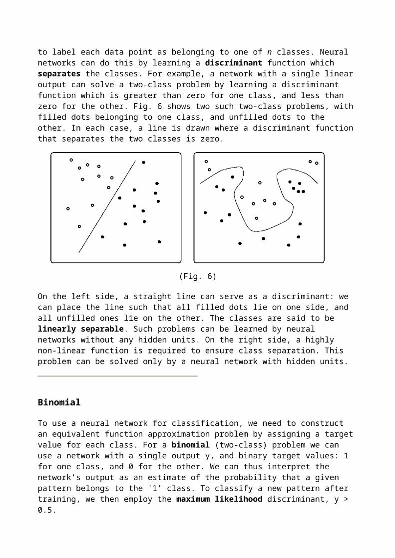
(8)

After the network has been presented with the whole series, we alter each weight wij by

(9)

We therefore need an algorithm that computes

(10)

at each time step t. Since we know ek(t) at all times (the difference between our targets and outputs),

we only need to find a way to compute the second factor .

IMPORTANT

The key to understanding RTRL is to appreciate what this factor expresses. It is essentially a measure of the sensitivity of the value of the output of unit k at time t to a small change in the value of wij, taking into account the effect of such a change in the weight over the entire network trajectory from t0 to t. Note that wij does not have to be connected to unit k. Thus this algorithm is non-local, in that we need to consider the effect of a change at one place in the network on the values computed at an entirely different place. Make sure you understand this before you dive into the derivation given next

Derivation of

This is given here for completeness, for those who wish perhaps to implement RTRL. Make sure

you at least know what role the factor plays in computing the gradient.

From Equations 2 and 3, we get

(11)

where is the Kronecker delta

(12)

[Exercise: Derive Equation 11 from Equations 2 and 3]

Because input signals do not depend on the weights in the network,

(13)

Equation 11 becomes:

(14)

This is a recursive equation. That is, if we know the value of the left hand side for time 0, we can compute the value for time 1, and use that value to compute the value at time 2, etc. Because we assume that our starting state (t = 0) is independent of the weights, we have

(15)

These equations hold for all .

We therefore need to define the values

(16)

for every time step t and all appropriate i, j and k. We start with the initial condition

pijk(t0) = 0 (17)

and compute at each time step

(18)

The algorithm then consists of computing, at each time step t, the quantities pijk(t) using equations

16 and 17, and then using the differences between targets and actual outputs to compute weight changes

(19)

and the overall correction to be applied to wij is given by

(20)

[Top] [Next: The dynamics of recurrent neural networks] [Back to the first page]

Dynamics and RNNs

Consider the recurrent network illustrated below. A single input unit is connected to each of the three "hidden" units. Each hidden unit in turn is connected to itself and the other hidden units. As in the RTRL derivation, we do not distinguish now between hidden and output units. Any activation which enters the network through the input node can flow around from one unit to the other, potentially forever. Weights less than 1.0 will exponentially reduce the activation, weights larger than 1.0 will cause it to increase. The non-linear activation functions of the hidden units will hopefully prevent it from growing without bound.

As we have three hidden units, their activation at any given time t describes a point in a 3-dimensional state space. We can visualize the temporal evolution of the network state by watching the state evolve over time.

In the absence of input, or in the presence of a steady-state input, a network will usually approach a fixed point attractor. Other behaviors are possible, however. Networks can be trained to oscillate in regular fashion, and chaotic behavior has also been observed. The development of architectures and algorithms to generate specific forms of dynamic behavior is still an active research area.

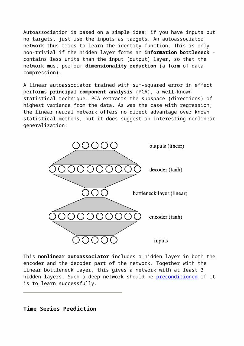
Some limitations of gradient methods and RNNs

The simple recurrent network computed a gradient based on the present state of the network and its state one time step ago. Using Back Prop Through Time, we could compute a gradient based on some finite n time steps of network operation. RTRL provided a way of computing the true gradient based on the complete network history from time 0 to the present. Is this perfection?

Unfortunately not. With feedforward networks which have a large number of layers, the weights which are closest to the output are the easiest to train. This is no surprise, as their contribution to the network error is direct and easily measurable. Every time we back propagate an error one layer further back, however, our estimate of the contribution of a particular weight to the observed error becomes more indirect. You can think of error flowing in the top of the network in distinct streams. Each pack propagation dilutes the error, mixing up error from distinct sources, until, far back in the network, it becomes virtually impossible to tell who is responsible for what. The error signal has become completely diluted.

With RTRL and BPTT we face a similar problem. Error is now propagated back in time, but each time step is exactly equivalent to propagating through an additional layer of a feed forward network. The result, of course, is that it becomes very difficult to assess the importance of the network state at times which lie far back in the past. Typically, gradient based networks cannot reliably use information which lies more than about 10 time steps in the past. If you now imagine an attempt to use a recurrent neural network in a real life situation, e.g. monitoring an industrial process, where data are presented as a time series at some realistic sampling rate (say 100 Hz), it becomes clear that these networks are of limited use. The next section shows a recent model which tries to address this problem.

[Top] [Next: Long Short-Term Memory] [Back to the first page]

Long Short-Term Memory

In a recurrent network, information is stored in two distinct ways. The activations of the units are a function of the recent history of the model, and so form a short-term memory. The weights too form a memory, as they are modified based on experience, but the timescale of the weight change is much slower than that of the activations. We call those a long-term memory. The Long Short-Term Memory model [1] is an attempt to allow the unit activations to retain important information over a much longer period of time than the 10 to 12 time steps which is the limit of RTRL or BPTT models.

The figure below shows a maximally simple LSTM network, with a single input, a single output, and a single memory block in place of the familiar hidden unit.

This figure below shows a maximally simple LSTM network, with a single input, a single output, and a single memory block in place of the familiar hidden unit. Each block has two associated gate units (details below). Each layer may, of course, have multiple units or blocks. In a typical configuration, the first layer of weights is provided from input to the blocks and gates. There are then recurrent connections from one block to other blocks and gates. Finally there are weights from the blocks to the outputs. The next figure shows the details of the memory block in more detail.

The hidden units of a conventional recurrent neural network have now been replaced by memory blocks, each of which contains one or more memory cells. At the heart of the cell is a simple linear unit with a single self-recurrent connection with weight set to 1.0. In the absence of any other input, this connection serves to preserve the cell's current state from one moment to the next. In addition to the self-recurrent connection, cells receive input from input units and other cell and gates. While the cells are responsible for maintaining information over long periods of time, the responsibility for deciding what information to store, and when to apply that information lies with an input and output gating unit, respectively.

The input to the cell is passed through a non-linear squashing function (g(x), typically the logistic function, scaled to lie within [-2,2]), and the result is then multiplied by the output of the input gating unit. The activation of the gate ranges over [0,1], so if its activation is near zero, nothing can enter the cell. Only if the input gate is sufficiently active is the signal allowed in. Similarly, nothing emerges from the cell unless the output gate is active. As the internal cell state is maintained in a linear unit, its activation range is unbounded, and so the cell output is again squashed when it is released (h(x), typical range [-1,1]). The gates themselves are nothing more than conventional units with sigmoidal activation functions ranging over [0,1], and they each receive input from the network input units and from other cells.

Thus we have:

Cell output: ycj(t) is

ycj(t) = yout

j(t) h(scj(t))

where youtj(t) is the activation of the output gate, and the state, scj(t) is given by

scj(0) = 0, and

scj(t) = scj(t-1) + yinj(t) g(netcj(t)) for t > 0.

This division of responsibility---the input gates decide what to store, the cell stores information, and the output gate decides when that information is to be applied---has the effect that salient events can be remembered over arbitrarily long periods of time. Equipped with several such memory blocks, the network can effectively attend to events at multiple time scales.

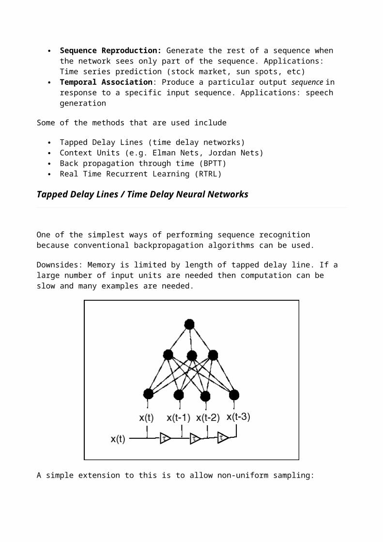
Network training uses a combination of RTRL and BPTT, and we won't go into the details here. However, consider an error signal being passed back from the output unit. If it is allowed into the cell (as determined by the activation of the output gate), it is now trapped, and it gets passed back through the self-recurrent connection indefinitely. It can only affect the incoming weights, however, if it is allowed to pass by the input gate.

On selected problems, an LSTM network can retain information over arbitrarily long periods of time; over 1000 time steps in some cases. This gives it a significant advantage over RTRL and BPTT networks on many problems. For example, a Simple Recurrent Network can learn the Reber Grammar, but not the Embedded Reber Grammar. An RTRL network can sometimes, but not always, learn the Embedded Reber Grammar after about 100 000 training sequences. LSTM always solves the Embedded problem, usually after about 10 000 sequence presentations.

One of us is currently training LSTM networks to distinguish between different spoken languages based on speech prosody (roughly: the melody and rhythm of speech).

References

Hochreiter, Sepp and Schmidhuber, Juergen, (1997) "Long Short-Term Memory", Neural Computation, Vol 9 (8), pp: 1735-1780

[Top] [Next: Projects] [Back to the first page]

Some possible project topics

The following are a few suggestions for project topics. They are all presented in a fiarly open-ended fashion here. Potential projects will need to be decided in detail depending on your interests and the size of the planned project. In each case, the final goals and requirements will have to be decided upon together with Professor Colombetti and us. You are also free to suggest topics of your own.

Please bear in mind that Nic and Fred are both normally in Lugano. They are, of course, contactable by email.

Implement Real Time Recurrent Learning (Neural Computation, 1, 270-280, 1989). Code up your own implementation of RTRL. Reproduce the results on temporal XOR and sine wave oscillation. Examine the effects of continuous and a discrete periodic inputs on a network trained to oscillate. In what way does the network entrain to an external signal?

8-3-8 Encoder Implement a feedforward network with one hidden layer and batch backpropagation, and either momentum or the bold driver method. Set it up as an autoencoder with 8 inputs/outputs and 3 hidden units, and train it on the 8 binary patterns that consist of a single '1' and 7 zeroes. Find values for the free parameters that give you fast, reliable convergence, then compare the speed of learning and ultimate performance for the following cases:

o linear outputs, sum-squared error o logistic outputs, sum-squared error o logistic outputs, cross-entropy error o softmax outputs, cross-entropy error

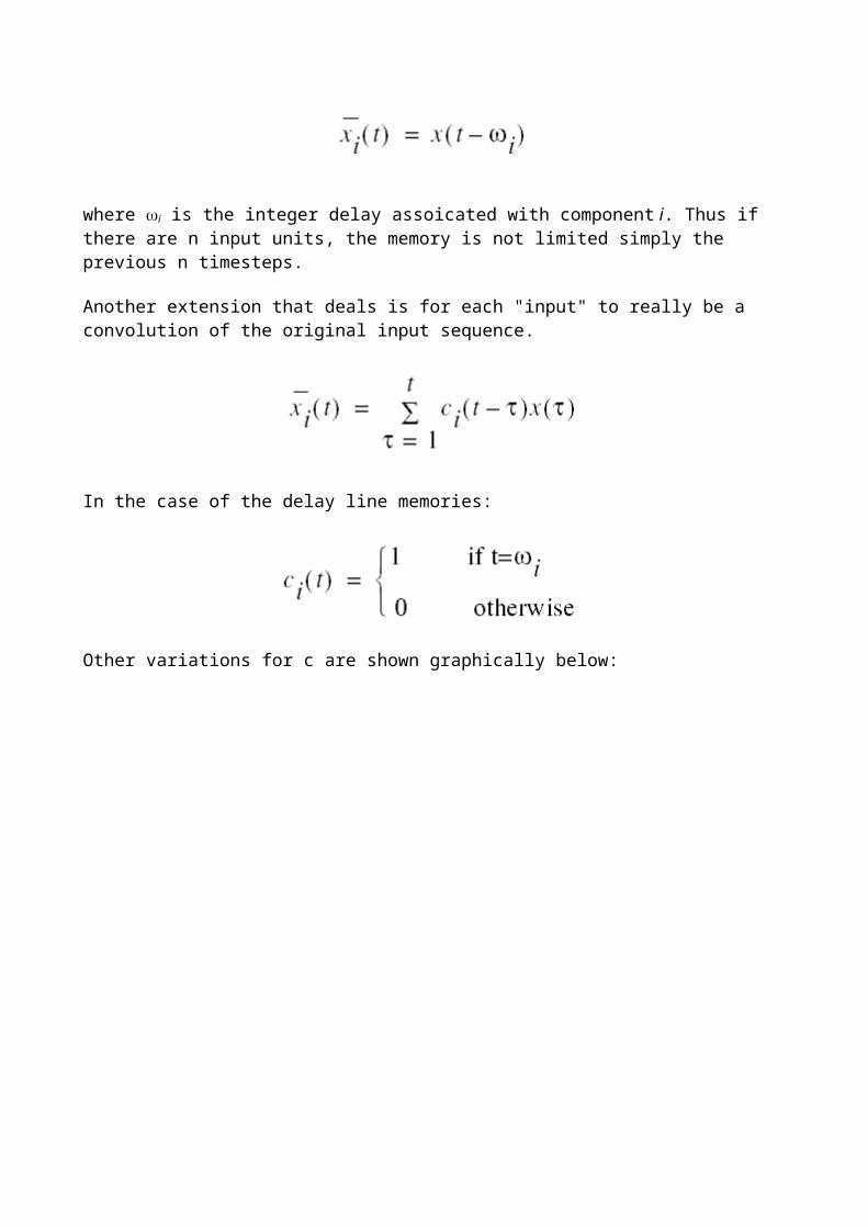
Online Learning Write a program that generates training data for a neural network, such that the function the network must learn to approximate changes periodically. Then implement a neural network that obtains its training patterns from this generator, and performs online learning with local learning rate adaptation on it. Compare the network's performance for various values of the meta-learning rate.

Tic-Tac-Toe Implement a network that uses Q-learning to learn the game of tic-tac-toe (see figure) from self-play.

Tic-tac-toe

Applications You may want to consider applying a neural network as part of a project that relates to other part of your course - for example, in building or simulating a reactive agent.

Your suggestion here. Have you a favourite dataset you wish to model? Time series data to predict? Pattern recognition problem? Let us know.

[Top] [Back to the first page]

Pattern Classification And Single Layer Networks: Chapter 2

Intro

We have just seen how a network can be trained to perform linear regression. That is, given a set of inputs (x) and output/target values (y), the network finds the best linear mapping from x to y.

Given an x value that we have not seen, our trained network can predict what the most likely y value will be. The ability to (correctly) predict the output for an input the network has not seen is called generalization.

This style of learning is referred to as supervised learning (or learning with a teacher) because we are given the target values. Later we will see examples of unsupervised learning which is used for finding patterns in the data rather than modeling input/output mappings.

We now step away from linear regression for a moment and look at another type of supervised learning problem called pattern classification. We start by considering only single layer networks.

Pattern classification

A classic example of pattern classifiction is letter recognition. We are given, for example, a set of pixel values associated with an image of a letter. We want the computer to determine what letter it is. The pixel values are refered to as the inputs or the decision variables, and the letter categories are referred to as classes.

Now, a given letter such as "A" can look quite different depending on the type of font that is used or, in the case of handwritten letters, different people's handwriting. Thus, there will be a range of values for the decision variables that map to the same class. That is, if we plot the values of the decision variables, different regions will correspond to different classes.

 

Example 1:

Two Classes (class 0 and class 1), Two Inputs (x1 and x2).

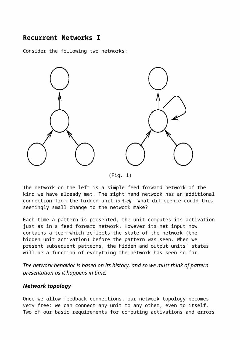
See also: Neural Java 2 Class Problem

Example 2:

Another example (see data description, data, Maple plots):class = types of irisdecision variables = sepal and petal sizes

Example 3:

example of zipcode digits in Maple

Single layer Networks for Pattern Classification

We can apply a similar approach as in linear regression where the targets are now the classes. Note that the outputs are no longer continuous but rather take on discrete values.

 Two Classes:

What does the network look like? If there are just 2 classes we only need 1 output node. The target is 1 if the example is in, say, class 1, and the target is 0 (or -1) if the target is in class 0. It seems reasonable that we use a binary step function to guarantee an appropriate output value.

Training Methods:

We will discuss two kinds of methods for training single-layer networks that do pattern classification:

Perceptron - guaranteed to find the right weights if they exist The Adaline (uses Delta Rule) - can easily be generalized to multi-layer nets (nonlinear

problems)

 

But how do we know if the right weights exist at all????

Let's look to see what a single layer architecture can do ....

Single Layer with a Binary Step Function

 Consider a network with 2 inputs and 1 output node (2 classes).

The net output of the network is a linear function of the weights and the inputs

net = W X = x1 w1 + x2 w2y = f(net)

 

 

x1 w1 + x2 w2 = 0 defines a straight line through the input space.

  x2 = - w1/w2 x1 <- this is line through the origin with slope -w1/w2

Bias

What if the line dividing the 2 classes does not go through the origin?

 

Other interesting geometric points to note:

The weight vector (w1, w2) is normal to the decision boundary.Proof: Suppose z1 and z2 are points on the decision boundary.

Linear Separability

Classification problems for which there is a line that exactly separates the classes are called linearly separable. Single layer networks are only able to solve linearly separable problems. Most real world are not linearly separable.

 

 

[Goto top of page] [Next: Perceptron] [Back to the first page]

The Perceptron 

The perceptron learning rule is a method for finding the weights in a network. We consider the problem of supervised learning for classification although other types of

problems can also be solved. A nice feature of the perceptron learning rule is that if there exist a set of weights that solve

the problem, then the perceptron will find these weights. This is true for either binary or bipolar representations.

Assumptions:

We have single layer network whose output is, as before,

output = f(net) = f(W X) where f is a binary step function f whose values are (+-1).

We assume that the bias treated as just an extra input whose value is 1 p = number of training examples (x,t) where t = +1 or -1

Geometric Interpretation:

With this binary function f, the problem reduces to finding weights such that

sign( W X) = t

That is, the weight must be chosen so that the projection of pattern X onto W has the same sign as the target t. But the boundary between positive and negative projections is just the plane W X = 0 , i.e. the same decision boundary we saw before.

The Perceptron Algorithm

1. initialize the weights (either to zero or to a small random value) 2. pick a learning rate ( this is a number between 0 and 1) 3. Until stopping condition is satisfied (e.g. weights don't change):

For each training pattern (x, t):

compute output activation y = f(w x) If y = t, don't change weights If y != t, update the weights:

w(new) = w(old) + 2 t x

or

w(new) = w(old) + (t - y ) x, for all t

Consider wht happens below when the training pattern p1 or p2 is chosen. Before updating the weight W, we note that both p1 and p2 are incorrectly classified (red dashed line is decision boundary). Suppose we choose p1 to update the weights as in picture below on the left. P1 has target value t=1, so that the weight is moved a small amount in the direction of p1. Suppose we choose p2 to update the weights. P2 has target value t=-1 so the weight is moved a small amount in the direction of -p2. In either case, the new boundary (blue dashed line) is better than before.

Comments on Perceptron

The choice of learning rate does not matter because it just changes the scaling of w. The decision surface (for 2 inputs and one bias) has equation:

x2 = - (w1/w2) x1 - w3 / w2

where we have defined w3 to be the bias: W = (w1,w2,b) = (w1,w2,w3)

From this we see that the equation remains the same if W is scaled by a constant.

The perceptron is guaranteed to converge in a finite number of steps if the problem is separable. May be unstable if the problem is not separable.

Come to class for proof!!

Outline: Find a lower bound L(k) for |w|2 as a function of iteration k. Then find an upper bound U(k) for |w|2. Then show that the lower bound grows at a faster rate than the upper bound. Since the lower bound can't be larger than the upper bound, there must be a finite k such that the weight is no longer updated. However, this can only happen if all patterns are correctly classified.

Perceptron Decision Boundaries

 

 

Two Layer Net: The above is not the most general region. Here, we have assumed the top layer is an AND function.

Problem: In the general for the 2- and 3- layers cases, there is no simple way to determine the weights.

[Top] [Next: Delta] [Back to the first page]

 

Delta Rule

Also known by the names:

Adaline Rule Widrow-Hoff Rule Least Mean Squares (LMS) Rule

Change from Perceptron:

Replace the step function in the with a continuous (differentiable) activation function, e.g linear

For classification problems, use the step function only to determine the class and not to update the weights.

Note: this is the same algorithm we saw for regression. All that really differs is how the classes are determined.

Delta Rule: Training by Gradient Descent Revisited

Construct a cost function E that measures how well the network has learned. For example

(one output node)

where

n = number of examples

ti = desired target value associated with the i-th example

yi = output of network when the i-th input pattern is presented to network

To train the network, we adjust the weights in the network so as to decrease the cost (this is where we require differentiability). This is called gradient descent.

Algorithm

Initialize the weights with some small random value Until E is within desired tolerance, update the weights according to

where E is evaluated at W(old), is the learning rate.: and the gradient is

 

More than Two Classes.

If there are mor ethan 2 classes we could still use the same network but instead of having a binary target, we can let the target take on discrete values. For example of there ar 5 classes, we could have t=1,2,3,4,5 or t= -2,-1,0,1,2. It turns out, however, that the network has a much easier time if we have one output for class. We can think of each output node as trying to solve a binary problem (it is either in the given class or it isn't).

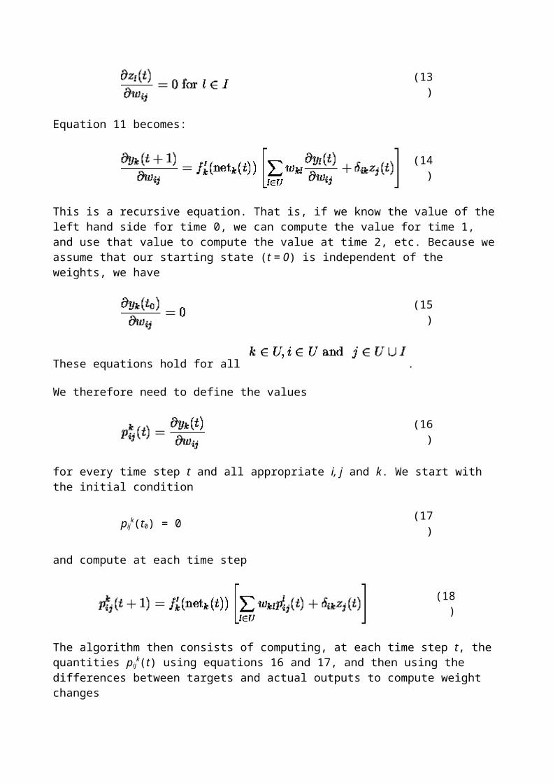
[Top] [Next: Correct] [Back to the first page]

Doing Classification Correctly

The Old Way

When there are more than 2 classes, we so far have suggested doing the following:

Assign one output node to each class. Set the target value of each node to be 1 if it is the correct class and 0 otherwise. Use a linear network with a mean squared error function. Determine the network class prediction by picking the output node with the largest value.

There are problems with this method. First, there is a disconnect between the definition of the error function and the determination of the class. A minimum error does not necessary produce the network with the largest number of correct prediction.

By varying the above method a little bit we can remove this inconsistency. Let us start by changing the interpretation of the output:

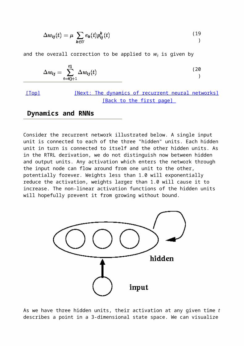
The New Way

New Interpretation: The output of yi is interpreted as the probability that i is the correct class. This means that:

The output of each node must be between 0 and 1 The sum of the outputs over all nodes must be equal to 1.

How do we achieve this? There are several things to vary.

We can vary the activation function, for example, by using a sigmoid. Sigmoids range continuously between 0 and 1. Is a sigmoid a good choice?

We can vary the cost function. We need not use mean squared error (MSE). What are our other options?

To decide, let's start by thinking about what makes sense intuitively. With a linear network using gradient descent on a MSE function, we found that the weight updates were proportional to the error (t-y). This seems to make sense. If we use a sigmoid activation function, we obtain a more complicated formula:

See derivatives of activation functions to see where this comes from.

This is not quite what we want. It turns out that there is a better error function/activation function combination that gives us what we want.

Error Function:

Cross Entropy is defined as

where c is the number of classes (i.e. the number of output nodes). 

This equation comes from information theory and is often applied when the outputs (y) are interpreted as probabilities. We won't worry about where it comes from but let's see if it makes sense for certain special cases.

Suppose the network is trained perfectly so that the targets exactly match the network output. Suppose class 3 is chosen. This means that output of node 3 is 1 (i.e. the probability is 1 that 3 is correct) and the outputs of the other nodes are 0 (i.e. the probability is 0 that class != 3 is correct). In this case do you see that the above equation is 0, as desired.

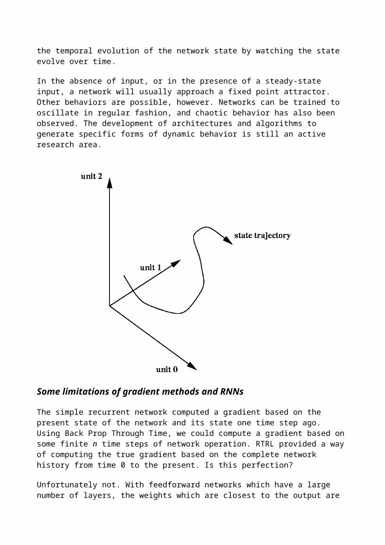
Suppose the network gives an output of y=.5 for all of the output i.e. that there is complete uncertainty about which is the correct class. It turns out that E has a maximum value in this case.

Thus, the more uncertain the network is, the larger the error E. This is as it should be. 

Activation function:

Softmax is defined as

where fi is the activation function of the ith output node and c is the number of classes.Note that this has the following good properties:

it is always a number between 0 and 1 when combined with the error function gives a weight update proportional to (t-y).

where ij = 0 if i=j and zero otherwise. Note that if r is the correct class then tr = 1 and RHS of the above equation reduces to (tr-yr)xs. If q!=r is the correct class then tr = 0 the above also reduces to (tr-yr)xs. Thus we have

Look familiar?

[Top] [Next: Optimizing] [Back to the first page]

Optimal Weight and Learning Rates for Linear Networks

Regression Revisited

 

Suppose we are given a set of data (x(1),y(1)),(x(2),y(2))...(x(p),y(p)):

If we assume that g is linear, then finding the best line that fits the data (linear regression) can be done algebraically:

The solution is based on minimizing the squared error (Cost) between the network output and the data:

where y = w x.

Finding the best set of weights

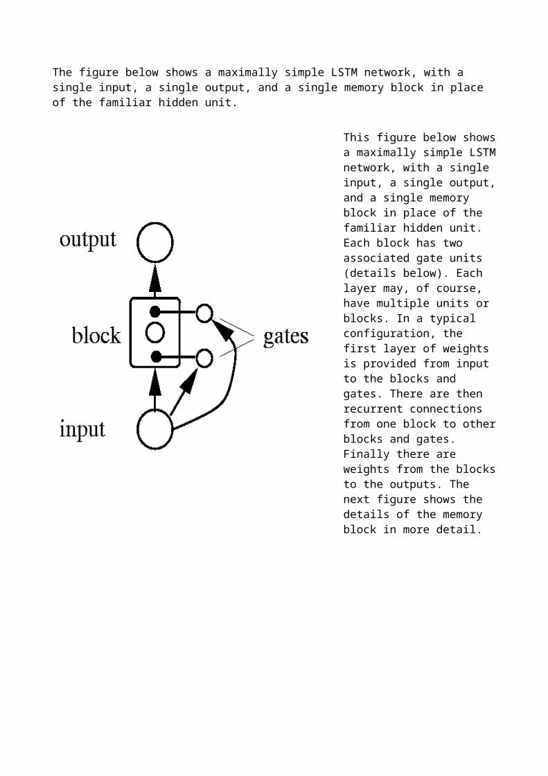
1-input, 1 output, 1 weight

But the derivative of E is zero at the minimum so we can solve for wopt.

n-inputs, m outputs: nm weights

The same analysis can be done in the multi-dimensional case except that now everything becomes matrices:

where wopt is an mxn matrix, H is an nxn matrix and Á is an mxn matrix.

Matrix inversion is an expensive operation. Also, if the input dimension, n, is very large then H is huge and may not even b possible to compute. If we are not able to compute the inverse Hessian or if we don't want to spend the time, then we can use gradient descent.

Gradient Descent: Picking the Best Learning Rate

 

For linear networks, E is quadratic then we can write

so that we have

But this is just a Taylor series expansion of E(w) about w0. Now, suppose we want to determine the optimal weight, wopt. We can differentiate E(w) and evaluate the result at wopt, noting that E`(wopt) is zero:

Solving for wopt we obtain:

comparing this to the update equation, we find that the learning "rate" that takes us directly to the minimum is equal to the inverse Hessian, which is a matrix and not a scalar. Why do we need a matrix?

2-D Example

 

 

Curvature axes aligned with the coordinate axes:

 

or in matrix form:

1 and 2 are inversely related to the size of the curvature along each axis. Using the above learning rate matrix has the effect of scaling the gradient differently to make the surface "look" spherical.

If the axes are not aligned with coordinate axes, the we need a full matrix of learning rates. This matrix is just the inverse Hessian. In general, H-1 is not diagonal. We can obtain the curvature along each axis, however, by computing the eigenvalues of H. Anyone remember what eigenvalues are??

Taking a Step Back

 

We have been spending a lot of time on some pretty tough math. Why? Because training a network can take a long time if you just blindly apply the basic algorithms. There are techniques that can improve the rate of convergence by orders of magnitude. However, understanding these techniques requires a deep understanding of the underlying characteristics of the problem (i.e. the mathematics). Knowing what speed-up techniques to apply, can make a difference between having a net that takes 100 iterations to train vs. 10000 iterations to train (assuming it trains at all).

The previous slides are trying to make the following point for linear networks (i.e. those networks whose cost function is a quadratic function of the weights):

1. The shape of the cost surface has a significant effect on how fast a net can learn. Ideally, we want a spherically symmetric surface.

2. The correlation matrix is defined as the average over all inputs of xxT 3. The Hessian is the second derivative of E with respect to w.

For linear nets, the Hessian is the same as the correlation matrix. 4. The Hessian, tells you about the shape of the cost surface: 5. The eigenvalues of H are a measure of the steepness of the surface along the curvature

directions. 6. a large eigenvalue => steep curvature => need small learning rate 7. the learning rate should be proportional to 1/eigenvalue 8. if we are forced to use a single learning rate for all weights, then we must use a learning rate

that will not cause divergence along the steep directions (large eigenvalue directions). Thus, we must choose a learning rate that is on the order of 1/»max where »max is the largest eigenvalue.

9. If we can use a matrix of learning rates, this matrix is proportional to H-1. 10. For real problems (i.e. nonlinear), you don't know the eigenvalues so you just have to guess.

Of course, there are algorithms that will estimate »max ....We won't be considering these here.

11. An alternative solution to speeding up learning is to transform the inputs (that is, x -> Px, for some transformation matrix P) so that the resulting correlation matrix, (Px)(Px)T, is equal to the identity.

12. The above suggestions are only really true for linear networks. However, the cost surface of nonlinear networks can be modeled as a quadratic in the vicinity of the current weight. We can then apply the similar techniques as above, however, they will only be approximations.

[Top] [Next: Summary] [Back to the first page]

Summary of Linear Nets

Characteristics of Networks

number of layers number of nodes per layer activation function (linear, binary, softwmax) error function (mean squared error (MSE), cross entropy) type of learning algorithms (gradient descent, perceptron, delta rule)

Types of Applications and Associated Nets

Regression:

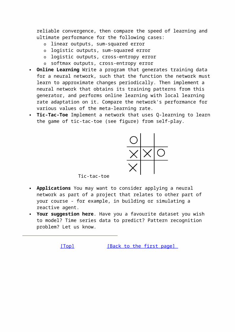
o uses a one-layer linear network (activation function is identity) o uses MSE cost function o uses gradient decent learning

Classification - Perceptron Learning o uses a one-layer network with a binary step activation function o uses MSE cost function o uses the perceptron learning algorithm (identical with gradient descent when targets

are +1 and -1) Classification - Delta Rule

o uses a one-layer network with a linear activation function o uses MSE cost function o uses gradient descent o the network chooses the class by picking the output node with the largest output

Classification - Gradient Descent (the right way) o uses a one-layer network with a softmax activation function o uses the cross entropy error function o outputs are interpreted as probabilities o the network chooses the class with the highest probability

Modes of Learning for Gradient Descent

Batch o At each iteration, the gradient is computed by averaging over all inputs

Online (stochastic) o At each iteration, the gradient is estimated by picking one (or a small number) of

inputs. o Because the gradient is only being esitimated, there is a lot of noise in the weight

updates. The error comes down quicly but then tends to jiggle around. To remove this noise one can switch to batch at the point where the error levels out and or to continue to use online but to decrease the learning rate (called annealing the learning rate). One way annealing is to use = 0/t where 0 us the originial learning rate and t is the number of timesteps after annealing is turned on.

Picking Learning Rates

Learning rates that are too big cause the algorithm to diverge Learning rates that are too small cause the algorithm to converge very slowly. The optimal learning rate for linear networks is /(H-1) where H is the Hessian and is

defined as the second derivative of the cost function with respect to the weights. Unfortunately, this is a matrix whose inverse can be costly to compute.

The best learning rate for batch is the inverse Hessian. More details if you are interested:

o The next best thing is to use a separate learning rate for each weight. If the Hessian is diagonal these learning rates are just one over the eigenvalues of the Hessian. Fat chance that the hessian is diagonal though!

o If using a single scalar learning then the best one to use is 1 over the largest eigenvalue of the Hessian. There are fairly inexpensive algorithms for estimating this. However, many people just use the ol' brute force method of picking the learning rate - trial and error.

o For linear networks the Hessian is < x xT> and is independent of the weights. For nonlinear networks (i.e. any network that has an activation function that isn't the identity), the Hessian depends on the value of the weights and so changes everytime the weights are updated - arrgh! That is why people love the trial and error approach.

Limitations of Linear Networks

For regression, we can only fit a straight line through the data points. Many problems are not linear.

For classification, we can only lay down linear boundaries between classes. This is often inadequate for most real world problems.

Where do we go next - Multilayer Nonlinear Networks!!!

[Top] [Next: Backprop] [Back to the first page]

Multilayer Networks and Backpropagation

 Introduction

Much early research in networks was abandoned because of the severe limitations of single layer linear networks. Multilayer networks were not "discovered" until much later but even then there were no good training algorithms. It was not until the `80s that backpropagation became widely known. People in the field joke about this because backprop is really just applying the chain rule to compute the gradient of the cost function. How many years should it take to rediscover the chain rule?? Of course, it isn't really this simple. Backprop also refers to the very efficient method that was discovered for computing the gradient.

 Note: Multilayer nets are much harder to train than single layer networks. That is, convergence is much slower and speed-up techniques are more complicated.

 Method of Training: Backpropagation

 Define a cost function (e.g. mean square error)

where the activation y at the output layer is given by

and where

z is the activation at the hidden nodes f2 is the activation function at the output nodes f1 is the activation function at the hidden nodes.

Written out more explicitly, the cost function is

or all at once:

Computing the gradient: for the hidden-to-output weights:

the gradient: for the input-to-hidden weights:

Summary of Gradients

hidden-to-output weights:

where

input-to-hidden:

where

Implementing Backprob

Create variables for :

the weights W and w, the net input to each hidden and output node, neti the activation of each hidden and output node, yi = f(neti) the "error" at each node, ´i

For each input pattern k:

Step 1: Foward Propagation

Compute neti and yi for each hidden node, i=1,..., h:

Compute netj and yj for each output node, j=1,...,m:

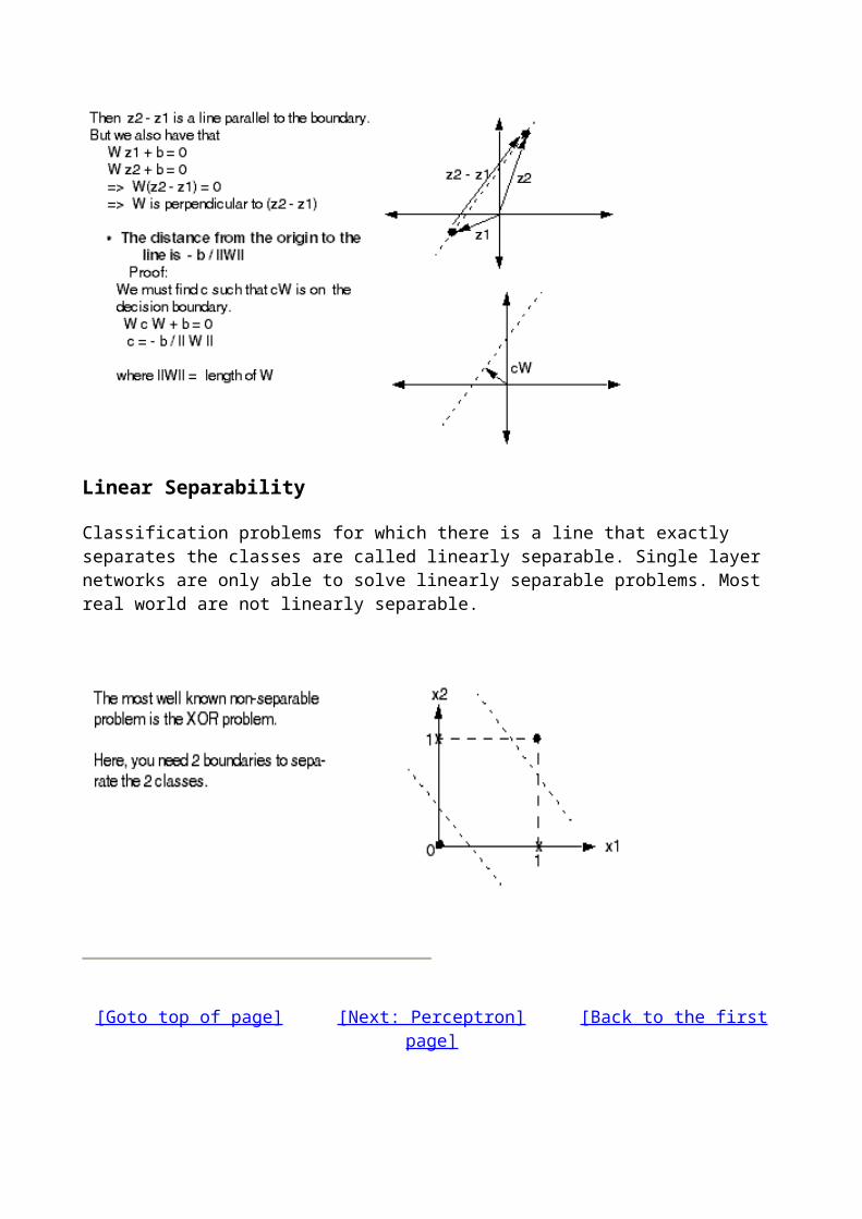
Step 2: Backward Propagation

Compute ´2's for each output node, j=1,...,m:

Compute ´1's for each hidden node, i=1,...,h

Step 3: Accumulate gradients over the input patterns (batch)

Step 4: After doing steps 1 to 3 for all patterns, we can now update the weights:

 

Networks with more than 2 layers

The above learning procedure (backpropagation) can easily be extended to networks with any number of layers.

[Top] [Next: Noise] [Back to the first page]

Online vs Batch for Non-Linear Networks

 Making a Lot of Noise

Disadvantage of Noise in Online Updates

We have seen that online can often be much faster than batch early in the training process. However, the noise in the updates causes the network to bounce around near the minimum and never converge to the very bottom.

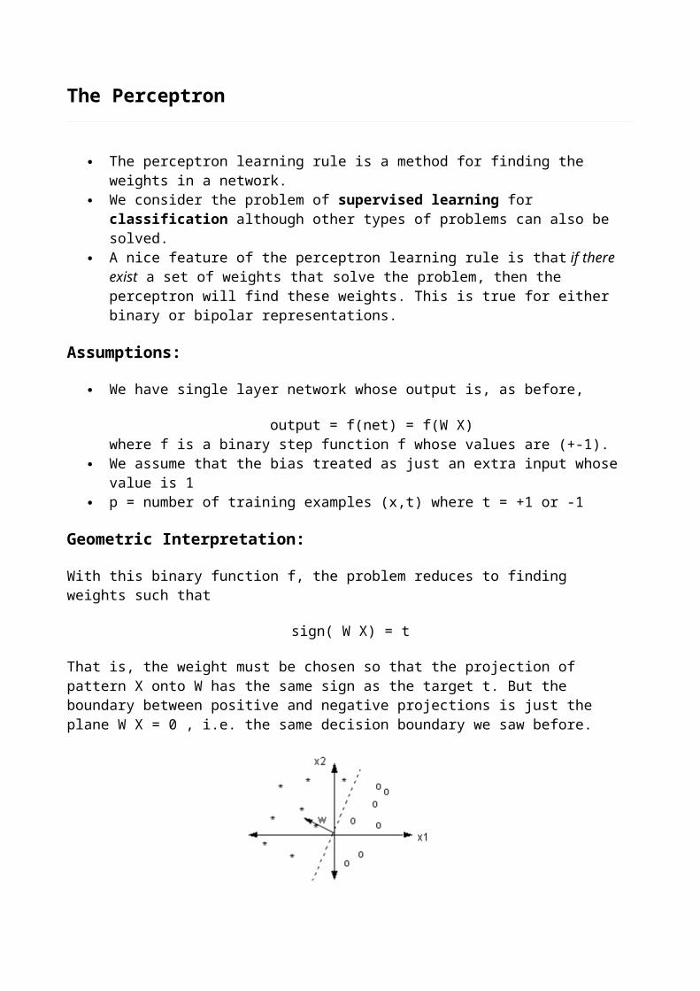
Solution:

The Advantage of Noise

In linear networks the cost function is in the nice shape of a bowl. There is a single minimum. In nonlinear networks, however, the cost surface can be very complex. There can be many minima, valleys, plateau's which make training very difficult. Batch gradient descent will simply move the bottom of the local minimum it randomly starts in. If it is on a plateau, the gradient may be very small and so learning takes a very long time. 

Valleys are common when using sigmoids. Consider what happens when sigmoids are added. Below, the green sigmoid is added to the blue to obtain the red.

Now, look what can happen in 2 dimensions. We obtain a valley that can be difficult to escape from: 

The noise in online makes it possible to escape from local minima and plateaus. It can help somewhat with valleys as well.

Too Much of a Good Thing: OverTraining

The good news is that multilayer networks can approximate any smooth function as long as you have enough hidden nodes. The bad news is that this added flexibility can cause the network to learn the noise in the data. Consider regression and classification problems where you have a collection of noisy data. The solid line is the "true" function or class boundary and the +'s and o's is the data:

If you have lots of hidden nodes you may find that the network "discovers" the function (dotted lines) given below:

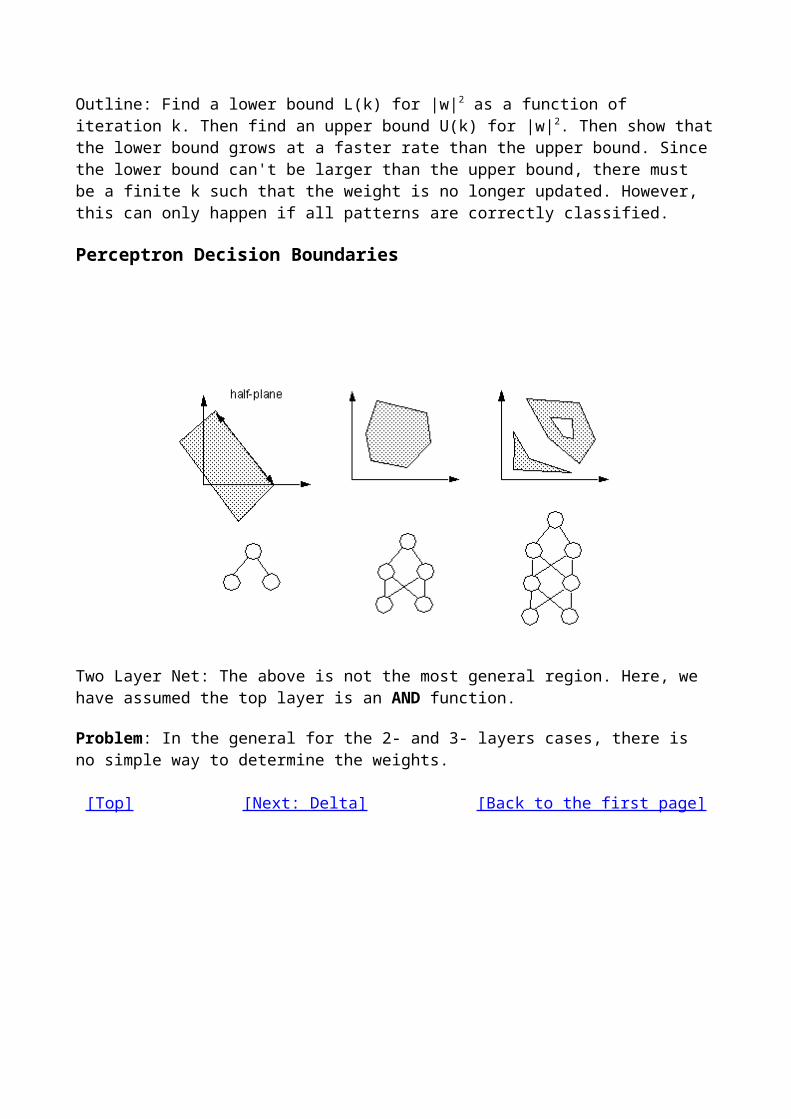
In the above example, the network has not only learned the function but it has also learned the noise present in the data. When the net has learned the noise, we say it has overtrained. The reason for this name is that as a net trains it first learns the rough structure of the data. As it continues to learn, it will pick up the details (i.e. the noise).

Generalization

Why is overtraining a problem? The whole purpose of training these nets is to be able to predict the function output (regression) or class (classification) for inputs that the net has never seen before (i.e. was not trained on).

A network is said to generalize well if it can accurately predict the correct output on data it has never seen.

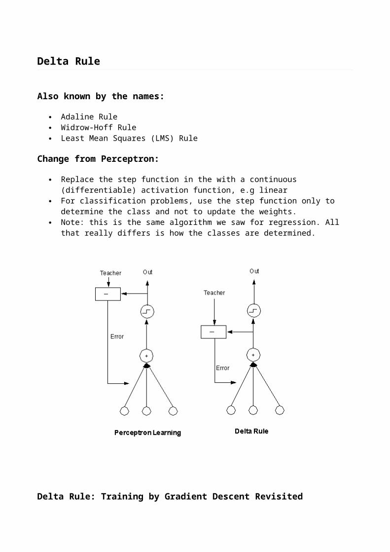
Preventing Overtraining

There are several ways to prevent overtraining:

training for less time. The method for doing this is called early stopping

Reducing the number of hidden nodes reduces the number or parameters (weights) so that the net is not able to learn as much detail. Problems are* what is the right number of nodes?* there is reason to believe that better solutions can be found by having toomany hidden nodes than too few.

Often, better to start with a big net, train, and then carefully prune the net so that it is smaller (one version of pruning is called optimal brain damage)

Instead of reducing the number of weights, people instead put constraints on the weights so that there are effectively fewer parameters. One example of this is weight decay.

Weight decay pushes the weights toward zero. Note that this corresponds to the linear region of the sigmoid

 [Top] [Next: Momentum] [Back to the first page]

Momentum

 

We saw that if the cost surface is not spherical, learning can be quite slow because the learning rate must be kept small to prevent divergence along the steep curvature directions

One way to solve this is to use the inverse Hession (= correlation matrix for linear nets) as the learning rate matrix. This can be problematic because the Hessian can be a large matrix that is difficult to invert. Also, for multilayer networks, the Hessian is not constant (i.e. it changes as the weights change). Recomputing the inverse Hessian at each iteration would be prohibitively expensive and not worth the extra computation. However a much simpler approach is to use the addition of a momentum term.

where w(t) is the weight at the tth iteration. Written another way

where w(t) = w(t)-w(t-1). Thus, the amount you change the weight is proportional to the negative gradient plus the previous weight change. is called the momentum parameter. and must satisfy 0 <= < 1.

Momentum Example

Consider the oscillatory behavior shown above. The gradient changes sign at each step. By adding in a small amount of the previous weight change, we can lessen the oscillations. Suppose = .8, w(0)=10E = w2 => wmin= 0 and dE/dx = 2w

No Momentum = 0:

t = 0: w(1) = -.8 = -.8 (20) = -16, w(1) = 10-16 = -6

t = 2: w(1) = -.8 = -.8 (-12) = 9.6, w(2) = -6+9.6 = 3.6

t = 3: w(1) = -.8 = - .8(7.2) = -5.76, w(2) = 3.6 - 5.76 = -2.16

 

With Momentum = .1:

t = 0: w(1) = -.8 + w(0) = -.8 (20) + .1*0 = -16, w(1) = 10-16 = -6

t = 2: w(1) = -.8 + w(1) = -.8 (-12) + .1*(-16) = 8, w(2) = -6+8 = 2

t = 3: w(1) = -.8 + w(2) = - .8(4) + .1*(8) = -2.4, w(2) = 2-2.4 = -.4

 

 

 [Top] [Next: DeltaBarDelta] [Back to the first page]

 Delta-Bar-Delta (Jacobs)

 Since the cost surface for multi-layer networks can be complex, choosing a learning rate can be difficult. What works in one location of the cost surface may not work well in another location. Delta-Bar-Delta is a heuristic algorithm for modifying the learning rate as training progresses:

Each weight has its own learning rate. For each weight: the gradient at the current timestep is compared with the gradient at the

previous step (actually, previous gradients are averaged) If the gradient is in the same direction the learning rate is increased If the gradient is in the opposite direction the learning rate is decreased Should be used with batch only.

Let

gij(t) = gradient of E wrt wij at time t

then define

Then the learning rate ij for weight wij at time t+1 is given by

where , , and are chosen by the hand.

Downsides: Knowing how to choose the parameters , , and is not easy.

Doesn't work for online.

 [Top] [Next: Unsupervised] [Back to the first page]  

Unsupervised Learning

Up until now we have discussed how to train nets given a training set of input and target values. The target value is often called the teacher signal because it represents the "right answer". i.e. what the output of the net should be. Training with a teacher signal is called supervised learning.

We can also train nets on inputs where there is no teacher signal. The purpose might be to

discover underlying structure of the data encode the data compress the data transform the data

This kind of learning is called unsupervised learning because there is no explicit teacher signal.

Examples of unsupervised learning

hebbian learning w(t+1) = w(t) + y(t) x(t) This moves w toward inifinity in the direction of the eigevector with largest eigenvalue of the correlation matrixA more stable version is Oja's rulew(t+1) = w(t) + (x(t) - y(t) w(t) ) y(t)

principal component analysis competitive learning vector quantization

 [Top] [Next: PCA] [Back to the first page]

Linear Data Compression

Goal: To find a low dimensional representation of the data

Example: Saving Space

 

In general, the data does not lie perfectly on a linear subspace. In this case, some information is lost when the data is compressed. The problem here is to find the compression direction that results in the least amount of information that is lost.

 

Principal Component Analysis (PCA)

The 1 direction corresponds to

the direction of largest variance of the data. the eigenvector associated with the largest eigenvalue of the correlation matrix ( <x xT> ).

If we have n dimensional data, we can compress it down to m dimensions by projecting it down to the space spanned by eigen vectors of the m largest eigenvalues.

The methods that can be used for finding these directions is called Principal Component Analysis (PCA).

Finding the Principal Components using an Autoassociative Network

An autoassociative network is a network whose inputs and targets are the same. That is, the net must find a mapping from an input to itself.

Why do this? Well, when the number of hidden nodes is smaller than the number of input node, the network is forced to learn an efficient low dimensional representation of the data.

 

See Maple example of the above network.

Example: Image Compression (Cottrell et al, 87)

64 inputs: 8x8 pixel regions of an image specified to 8 bit precision 16 hidden units 64 outputs: targets = inputs 

Trained on randomly selected patches of an image (150,000 training steps). It was then tested on the entire image patch by patch using the entire set of non overlapping patches See "Fundamentals of Artificial Neural Networks", Hassoun, pp247-253.

They found that nonlinearity in the hidden units gave no advantage (this was later confirmed theoretically).

 [Top] [Next: NonlinearPCA] [Back to the first page]

Nonlinear Compression Techniques

Two layer networks perform a projection of the data onto a linear subspace. In this case, the encoding and decoding portions of the network are really single layer linear networks.

This works well in some cases. However, many datasets lie on lower dimensional subspaces that are not linear.

Example:

A helix is 1-D, however, it does not line on a 1-D linear subspace.

 

To solve this problem we can let the encoding and decoding portions each be multilayer networks. In this way we obtain nonlinear projections of the data.

5-Layer Networks:

Example: Hemisphere

(from Fast Nonlinear Dimension Reduction, Nanda Kambhatla,NIPS93)

Compressing a hemisphere onto 2 dimensions

 

 Example: Faces

(from Fast Nonlinear Dimension Reduction, Nanda Kambhatla,NIPS93)

In the examples below, the original images consisted of 64x64 8-bit/pixel grayscale images. The first 50 principal components were extracted to from the image you see on the left. This was reduced to 5 dimensions using linear PCA to obtain the image in the center. The same imageon the left was also reduced to 5 dimensions using a 5-layer (50-40-5-40-50) network to produce the image on the right.

Face 1:

50 principal components 5 principal components 5 nonlinear components

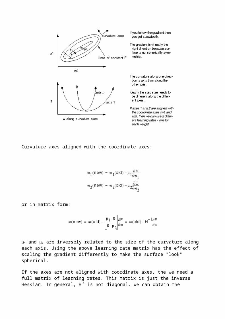
Face 2:

50 principal components 5 principal components 5 nonlinear components

 [Top] [Next: Competitive] [Back to the first page]

Simple Competitive Learning

In competitive networks, output units compete for the right to respond.

Goal: method of clustering - divide the data into a number of clusters such that the inputs in the same cluster are in some sense similar.

A basic competitive learning network has one layer of input nodes and one layer of output nodes. Binary valued outputs are often (but not always) used. There are as many output nodes as there are classes.

Often (but not always) there are lateral inhibitory connections between the output nodes.(in simulations, the function of the lateral connections can be replaced with a different algorithm)

The output units are also often called grandmother cells. The term grandmother cell comes from discussions as to whether your brain might contain cells that fire only when you encounter your maternal grandmother, or whether such higher level concepts are more distributed.

Vector Quantization (VQ)

Vector quantization is one example of competitive learning.

The goal here is to have the network "discover" structure in the data by finding how the data is clustered. The results can be used for data encoding and compression. One such method for doing this is called vector quantization.

In vector quantization, we assume there is a codebook which is defined by a set of M prototype vectors. (M is chosen by the user and the initial prototype vectors are chosen arbitrarily).

An input belongs to cluster i if i is the index of the closest prototype (closest in the sense of the normal euclidean distance). This has the effect of dividing up the input space into a Voronoi tesselation

.

Implementing Vector Quantization with a Network

 

Algorithm: Choose the number of clusters M Initialize the prototypes w*1,... w*m (one simple method for doing this is to randomly choose

M vectors from the input data) Repeat until stopping criterion is satisfied:

o Randomly pick an input x o Determine the "winning" node k by finding the prototype vector that satisfies

| w*k - x | <= | w*i - x | ( for all i )

note: if the prototypes are normalized, this is equivalent to maximizing w*i x o Update only the winning prototype weights according to

w*k(new) = w*k(old) + ( x - w*k(old) )

This is called the standard competitive learning rule

See Maple Example.

VQ and Data Compression

Vector quantization can be used for (lossy) data compression. If we are sending information over a phone line, we

initially send the codebook vectors for each input, we send the index of the class that the input belongs

For a large amount of data, this can be a significant reduction. If M=64, then it takes only 6 bits to encode the index. If the data itself consists of floating point numbers (4 bytes) there is an 80% reduction ( 100*(1 - 6/32) ).

Learning Vector Quantization (LVQ)

This is a supervised version of vector quantization. Classes are predefined and we have a set of labelled data. The goal is to determine a set of prototypes the best represent each class.

 [Top] [Next: Kohonon] [Back to the first page]

Kohonen's Self-Organizing Map (SOM)

Kohonon's SOMs are a type of unsupervised learning. The goal is to discover some underlying structure of the data. However, the kind of structure we are looking for is very different than, say, PCA or vector quantization.

Kohonen's SOM is called a topology-preserving map because there is a topological structure imposed on the nodes in the network. A topological map is simply a mapping that preserves neighborhood relations.

In the nets we have studied so far, we have ignored the geometrical arrangements of output nodes. Each node in a given layer has been identical in that each is connected with all of the nodes in the upper and/or lower layer. We are now going to take into consideration that physical arrangement of these nodes. Nodes that are "close" together are going to interact differently than nodes that are "far" apart.

What do we mean by "close" and "far"? We can think of organizing the output nodes in a line or in a planar configuration.

The goal is to train the net so that nearby outputs correspond to nearby inputs.

E.g. if x1 and x2 are two input vectors and t1 and t2 are the locations of the corresponding winning output nodes, then t1 and t2 should be close if x1 and x2 are similar. A network that performs this kind of mapping is called a feature map.

In the brain, neurons tend to cluster in groups. The connections within the group are much greater than the connections with the neurons outside of the group. Kohonen's network tries to mimick this in a simple way.

Algorithm for Kohonon's Self Organizing Map

Assume output nodes are connected in an array (usually 1 or 2 dimensional) Assume that the network is fully connected - all nodes in input layer are connected to all

nodes in output layer. Use the competitive learning algorithm as follows:

Randomly choose an input vector x Determine the "winning" output node i, where wi is the weight vector connecting the inputs

to output node i.Note: the above equation is equivalent to wi x >= wk x only if the weights are normalized.

Given the winning node i, the weight update is

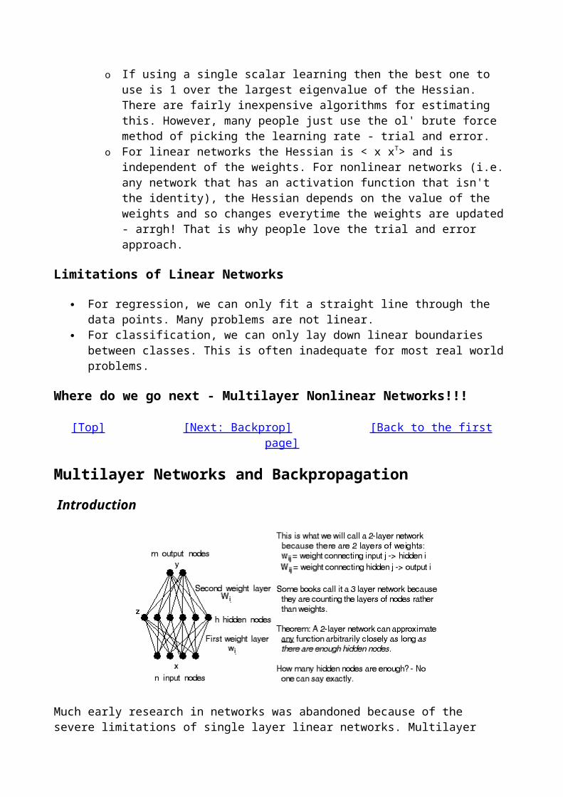
where is called the neighborhood function that has value 1 when i=k and falls off with the distance |rk - ri | between units i and k in the output array. Thus, units close to the winner as well as the winner itself, have their weights updated appreciably. Weights associated with far away output nodes do not change significantly. It is here that the toplogical information is supplied. Nearby units receive similar updates and thus end up responding to nearby input patterns.

The above rule drags the weight vector wi and the weights of nearby units towards the input x.

Example of the neighborhood function is:

where 2 is the width parameter that can gradually be decreased over time.

 [Top] [Next: RL] [Back to the first page]

Reinforcement Learning

Learning with a Critic

In supervised learning we have assumed that there is a target output value for each input value. However, in many situations, there is less detailed information available. In extreme situations, there is only a single bit of information after a long sequence of inputs telling whether the output is right or wrong. Reinforcement learning is one method developed to deal with such situations.

Reinforcement learning (RL) is a kind of supervised learning in that some feedback from the environment is given. However the feedback signal is only evaluative, not instructive. Reinforcement learning is often called learning with a critic as opposed to learning with a teacher.

Learning from Interaction

Humans learn by interacting with the environment. When a baby plays, it waves its arms around, touches things, tastes things, etc. There is no explicit teacher but there is a sensori-motor connection to its environment. Such a connection provides information about cause and effect, the consequence of actions, and what to do to achieve goals.

Learning from interaction with our environment is a fundamental idea underlying most theories of learning.

RL has rich roots in the psychology of animal learning, from where it gets its name.

The growing interest in RL comes in part from the desire to build intelligent systems that must operate in dynamically changing real- world environments. Robotics is the common example.

Environment

In RL, it is common to think explicitly of a network functioning in an environment. The environment supplies inputs to the network, receives output, and then provides a reinforcement signal.

In the most general case, the environment may itself be governed by a complicated dynamical process. Both reinforcement signals and input patterns may depend arbitrarily on the past history of the networks's output.

The classic problem is in game theory, where the "environment" is actually another player or players.

Temporal Credit Assignment Problem

A network designed to play chess would receive a reinforcement signal (win or lose) after a long sequence of moves. The question that arises is: How do we assign credit or blame individually to each move in a sequence that leads to an eventual victory or loss?

This is called the temporal credit assignment problem in contrast with the structural credit problem where we must attribute network error to different weights.

Learning and Planning

So far in this course we have not discussed the issue of planning. The networks we have seen are simply learning a direct relationship between an input and an output. RL is our first look at networks that in some sense decide a course of action by considering possible future actions before they are actually experienced.

Related Work

RL is closely related to

dynamic programming methods state-space planning methods used in AI

Exploration vs Exploitation

RL is learning what to do - how to map situations to actions - so as to maximize a scalar reward signal.

There are two important features:

trial-and-error search: the learner is not told what actions to take

delayed reward: actions can affect not only the immediate reward but also all subsequent rewards

There is always a trade-off in

exploration: discovery new actions, and exploitation: using what it currently knows to obtain the a reward

 [Top] [Next: Components] [Back to the first page]

Components of Reinforcement Learning

Reinforcement learning has 3 basic components:

agent: the learner or the decision maker environment: everything the agent interacts with, i.e. everything outside the agent actions: what the agent can do.

Each action is associated with a reward. The objective is for the agent to choose actions so as to maximize the expected reward over some period of time.

Example: The n-Armed Bandit

Java Simulation

There are n levers that can be pulled.

The action at each step is to choose a lever to pull.

The rewards are the payoffs for hitting the jackpot. Each arm has some average reward, called it's value. If you know the value then the solution is trivial: always pick the lever with the largest value.

What if you don't know the values of any of the arms? What is the best approach for estimating the value while at the same time maximizing your reward?

Greedy Approach: Policy: Always pick the arm with the largest estimated value. This is called exploiting your current knowledge.

Non-Greedy Approach: If you select a nongreedy approach then you are said to be exploring.

Balanced Approach: Choose a balance between exploration and exploitation. The balance partly depends on how many plays you get. If you have 1 play then the best approach is exploitation. However, there are many plays you will need some combination. The reward will be lower in the short term but higher in the long run.

Let:

Q*(a) = true actual value of taking an action a

Qt(a) = estimated value of taking an action a = (sum of rewards)/(number of steps)

As t->infinity, Qt(a) -> Q*(a)

Example: A simple policy would be to take the greedy choice most of the time but every now and then (with probability e), randomly select an action. How do we choose e? select

Components of the Agent

A reinforcement learning agent generally has 4 basic components:

a policy, a reward function, a value function, and a model of the environment

Policy

The policy is the decision making function of the agent. It specifies what action the agent should take in any of the situations it might encounter. This is the core of the agent. The other components serve only to change and improve the policy.

Reward Function

The reward function defines the goal of the RL agent. It maps the state of the environment to a single number, a reward, indicating the intrinsic desirability of the state. The agent's objective is to maximize the total reward it receives in the long run.

Value function

The value function specifies what is good in the long run. Roughly speaking, the value of a state is the total amount of reward the agent can expect to accumulate over the future when starting from the current state.

Rewards determine immediate desirability while value indicates the long term desirability.

In analogy to humans, rewards are immediate pleasure (if high reward) or pain (if low) whereas values correspond to more refined far-sighted judgement of how pleased or displeased we are that our environment is in a particular state.

Most of the methods we will discuss are centered around forming and improving approximate value functions.

Model

The model of the environment or external world should mimic the behavior of the environment. For example, given a situation and action, the model might predict the resultant next state and next reward. The model often takes up the largest storage space. If there are S states and A actions then a

complete model will take up a space proportional to S x S x A because it maps state-action pairs to probability distributions over states. By contrast, the reward and value functions might just map states to real numbers and thus be of size S.

 [Top] [Next: Terminology] [Back to the first page]

Terminology

Reinforcement Learning is about learning a mapping from states to a probability distribution over actions. This is called the policy. 

Policy = (s,a) = probability of taking action a when in state s

S = set of all states (assume finite)

st = state at time t

A(st) = set of all possible actions given agent is in state st S

at = action at time t

rt R (reals) = reward at time t

At each timestep t=1,2,3,...

the agent finds itself in a state st S and on that basis chooses an action at A(st). One timestep later, the agent receives a reward rt+1 and finds itself in a new state st+1.

The return, rett, is the total reward received starting at time t+1:

rett= rt+1 + rt+2 + rt+3 .... + rf

where rf is the reward at the final time step (can be infinite)

and the discounted return is

rett= rt+1 + rt+2 + 2 rt+3 ....

where 0 <= <= 1 is called the discount factor.

We assume that the number of states and actions is finite. We then define the state transition probabilities to be:

This is just the probability of transitioning from state s to state s' when action a has been taken.

Expected Rewards

The value function for policy is

The action-value function for policy is

Bellman's Equation for V(s) (Recursion on V(s)) is

 

Bellman Optimality Equations

Goal: Find the policy that gives the greatest return over the long run. We say a policy is better than or equal to policy ' if V(s) >= V'(s) for all s. There is always at least one such policy. Such a policy it is called an optimal policy and is denoted by *. Its corresponding value function is called V*:

V*(s) = V*(s) = max_ V(s) , for all s

and the optimal action-value function

Q*(s,a) = Q*(s,a) = max_ Q(s,a) , for all s, a

The Bellman optimality equation is then

This equation has a unique solution. It is a system of equations with |S| equations and |S| unknowns. If P and R were known then, in principle, it can be solved using some method for solving systems of nonlinear equations. Once V* is known, the optimal policy is determined by always choosing the action that produces the largest V*.

 [Top] [Next: ] [Back to the first page]

Summary of Nonlinear Networks and Applications

Backpropagation

Implementing backprop characteristics of cost surfaces

Activation Functions

linear threshold: binary, bipolar sigmoid: bipolar (symmetric), sigmoid softmax

Cost Functions

Mean Squared Error (MSE) Cross Entropy

Improving Generalization

using noise to improve learning, annealing what does it mean to overtrain? early stopping weight decay pruning (e.g. optimal brain damage)

Speed-up Techniques

momentum delta-bar-delta

Unsupervised Learning

Dimension Reduction for Compression using Autoassociative Networks o Principal Component Analysis (PCA) using 3 layer nets o Nonlinear PCA using 5-layer nets

Clustering for Compression Kohonen's Self-Organizing Maps (SOMs)

Misc Terminology

correlation matrix vs Hessian linear separability bias decision boundary clustering dimension reduction overtraining

Experimental Design

What techniques would you use to understand the data? (graphing data, examining correlation matrix, dimension reduction,...)

What type of architecture would you use? (number of layers, number of nodes, activation functions) Why?

What learning algorithm would you use (speed-up technique)? Why? What do you do to insure the net is trained adequately? (but not overtrained)

http://diwww.epfl.ch/w3mantra/tutorial/english/index.html

 

Neural Java 

    Neural Networks Tutorial with Java Applets Introduction

Neural Java is a series of exercises and demos. Each exercise consists of a short introduction, a small demonstration program written in Java (Java Applet), and a series of questions which are intended as an invitation to play with the programs and explore the possibilities of different algorithms.

The aim of the applets is to illustrate the dynamics of different artificial neural networks. Emphasis has been put on visualization and interactive interfaces. The Java Applets are not intended for and not useful for large-scale applications! Users interested in application programs should use other simulators.

The list below covers standard neural network algorithms like BackProp, Kohonen, and the Hopfield model. It also includes some models that are more biological, and features visualizations of the Hodgkin-Huxley and the integrate-and-fire models.

Additional material

The following are available for download:

Spiking Neuron Models (W. Gerstner and W. Kistler, Cambridge University Press 2002) Supervised Learning for Neural Networks: a tutorial with JAVA exercises (W. Gerstner).

See also

Some Competitive Learning Methods (Bernd Fritzke)

Exercises

If there is this image on the right of the link, then you can download the applet in order to

execute it at your place. And if there is this image on the right of the link, then you can download the source code of the applet. But you must agree before with the GNU General Public Licence.If so follow the instructions here to download and install the applets.

Single Neurons

1. Artificial Neuron .  

2. McCulloch-Pitts Neuron .  

3. Spiking Neuron. (Requires Swing).  

4. Hodgkin-Huxley Model .  

5. Axons and Action Potential Propagation .  

Supervised Learning

Single-layer networks (simple perceptrons)

1. Perceptron Learning Rule .  

2. Adaline, Perceptron and Backpropagation .  

Multi-layer networks

1. Multi-layer Perceptron (with neuron outputs in {0;1}) .  

2. Multi-layer Perceptron (with neuron outputs in {-1;1}) .  

3. Multi-layer Perceptron and C language .

4. Generalization in Multi-layer Perceptrons (with neuron outputs in {0;1}) .  

5. Generalization in Multi-layer Perceptrons (with neuron outputs in {-1;1}) .

 

6. Optical Character Recognition with Multi-layer Perceptron .  

7. Prediction with Multi-layer Perceptron .  

Density Estimation and Interpolation

1. Radial Basis Function Network .  

2. Gaussian Mixture Model / EM .  

3. Mixture model, using unlabeled data

Unsupervised Learning

1. Principal Component Analysis .   2. PCA for Character Recognition.

3. Competitive Learning Methods .  

Reinforcement Learning

1. Blackjack and Reinforcement Learning .  

Network DynamicsHopfield Network.

1. Pseudoinverse Network .  

2. Network of spiking neurons . (Requires Swing).  

3. Retina Simulation . (Runs very slow with some netscape versions).  

Miniproject

Miniproject for Postgraduate Training

Useful links

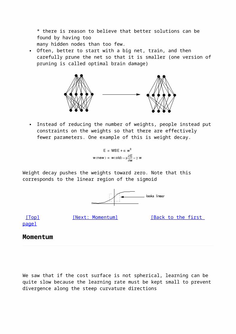
URL: http://diwww.epfl.ch/mantra/tutorial/english/ Last updated: 06-October-2000 by Sébastien Baehni

http://www.leemon.com/websim/index.html

WebSim 1.30 Home | Machine Learning | Crypto | Graphics

Publications | Concise Pubs | BibTeX Pubs | Other Pubs | WebSim

OverviewDemosMore Complex DemosSpeed ImprovementsDownloadWhere to get more information

Overview4 July 1998:     WebSim is a general simulator for neural networks, reinforcement learning, fractals, etc. WebSim has been designed for extendability, so it is easy to more more functions as needed. WebSim modules now exist so that a simulation can be performed by using any combination of the following modules:

Learning Algorithms: supervised learning, TD(Lambda), Q-learning, value iteration, advantage learning

Function approximators: lookup table, linear function approximator, multilayer perceptron (with a wide variety of squashing functions), radial basis functions (also with a wide variety of squashing functions), These can also be combined in series, and the they all know how to calculate both gradients and Hessians for those learning algorithms that use first or second derivatives.

Gradient-descent methods: backprop (with momentum), conjugate gradient. These can run in either incremental mode (changing weights after each training example), epoch-wise (changing after one pass through all examples), or in batches (changing after each N examples). These can either use the true gradient (residual gradient algorithms), a false gradient ignoring generalization in the function approximator (direct algorithms) or a linear combination in between (residual algorithms).

Graphics: 2D plots, 3D plots, contour plots. These can show the function learned, the value function learned (optimal Q-value/Advantage in each state), or the policy.

WebSim is best viewed under a JDK 1.1 browser, rather than JDK 1.0. This means that Netscape 4.05 will not work, but Netscape 4.06 and higher will work. Recent versions of MSIE and HotJava also work fine.

WebSim Demosbackprop learning of a nonlinear function by a sigmoidal multilayer perceptrongradient descent on the sum of two mean-squared-error functions to satisfy both simultaneously.conjugate gradient learning of an ill-conditioned linear function by a linear function approximatorValue Iteration demo.Gridworld experiment with a lookup table.show the names of all threads that are currently running.

Grids that can be used as backgrounds for 2D plots in WebSim.3D VRML scene controlled by a WebSim experiment. This works with Netscape using the

Cosmo Player beta 3a plugin. Both beta 5 and beta 3a are available for download, but only beta 3a has supports Java. This beta Cosmo is slow and crashes frequently, but it does give a hint of what the final realease will look like.

More Complex DemosThe following examples require security privileges that may not be available on all Java systems. For example, one that writes to a file on the hard drive will work under the JDK or Cafe or HotJava, but not under the current version of Netscape or Internet Explorer.

Create a short summary BNF description of the language WebSim parses, and send it to standard out (requires access to the hard drive).

Create a long, well-commented BNF description of the language WebSim parses, and send it to standard out (requires access to the hard drive).

Create a sequence of GIFs showing the 3D graph change as backprop learns a nonlinear function (requires accesss to the hard drive).

Load a data set from the Internet and do supervised learning on it. (requires security settings that allow ftp connections to the University of California at Irvine).

Speed ImprovementsWebSim is fast under the WinNT Symantec jit version 2.0 (beta 33). The slowest part of the code will be something like a large matrix multiply. For some matrix operations, Java is as fast as C, and for others it is slower. On tasks such as graphics, Internet and file access, and most math operations, Java will be as fast as optimized C, since those operations are done in either the operating system or the Java runtime libraries which are written in C. The Symantec jit has been liscensed by Netscape for their browser and Sun for its JDK, so this type of speed should soon be widely available, at least on PCs. Since a machine-learning problem with a large neural net spends most of its time in the matrix library, it can be useful to have WebSim use compiled C code for the matrix operations. WebSim has been written to automatically check to see if it is in a runtime environment that allows native code (precompiled C code) to be linked in, and if so it automatically checks the hard drive to see if there is any matrix code there. If there is, it automatically uses that for all the matrix operations, increasing their speed for some operations. To use this feature, you don't have to modify WebSim; simply place the compiled code at the appropriate place on the hard drive. On a PC, download Matrix.DLL into the directory c:\windows (for Win3.1 or Win95) or c:\WinNT.0 (for WinNT). That's it. The code will automatically be used by WebSim. WebSim will not have to be changed to use native code on other platforms. To go back to pure Java, just rename the DLL file or move it to another directory. The source is in this directory and is plain ANSI C, so it can be compiled for any platform using the .h files that come with the JDK or Cafe.

DownloadThe following information about WebSim is currently available for download or reading online:

The full source codeThe automatically-generated documentation for the source codeThe short and long BNF description of the WebSim language.An intro to writing WebSim classesThe code revision history

zip file containing all of the above.WebSim is best viewed under a JDK 1.1 browser, rather than JDK 1.0. Most browsers (including

MSIE and Hot Java) are 1.1. The standard Netscape 4.05 browser is still 1.0, but a 1.1 version of Netscape 4.05 is available for free download.

Where to Get More Information

This version of WebSim is equivalent to a late beta; it doesn't crash, but it is still undergoing major changes. This code is (c) 1996-1998 by the respective authors, is freeware, and may be freely distributed. If modifications are made, please say so in the comments. WebSim was designed and the core code was written by Leemon Baird. Other major portions of WebSim were written by Mance Harmon, Scott Weaver, and Ansgar Laubsch. WebSim also uses freeware utility code downloaded from the Web, including Nicholas Paldino's ftp code, Ernest Friedman-Hill's Postscript saving code, and Jef Poskanzer's GIF saving code. See their Web sites for restrictions on the use of their code. If you find WebSim useful, please send e-mail to Mance Harmon so he can keep everyone informed as changes are made. If you write new WebSim modules and are willing to make them freeware too, let him know and we'll add them to this archive or add a link to your archive.