jnasci.orgjnasci.org/wp-content/uploads/noid-solving_linear_fuzzy... · web viewin this paper,...
TRANSCRIPT

Artificial bee colony algorithm for solving linear fuzzy Fredholm integral equation of the second kind
M . Hasani ,a B . Asadya , M . Alavia
aDepartment of mathematics, Science and Research branch, Islamic Azad University, Hamadan,
Iran.
Abstract
In this paper, we propose a new method to solve fuzzy Fredholm integral equations(FFIE) by using artificial bee
colony algorithm. In this approach, ABC algorithm is employed as the main optimizer for optimal adjustments of
error control variables of the(FFIE) solution. The ability of artificial bee colony algorithm in function approximation
is our main objective. Also, we offering some numerical examples to illustrate capability and robustness, of the
presented method .
Keywords: Fuzzy numbers, Fuzzy Fredholm integral equations, Artificial bee colony algorithm
1

1 Introduction
Since many mathematical formulations of physical phenomena contain fuzzy integral equations and so these
equations are very useful for solving many problems in several applied fields like mathematical physics and
engineering. Also, these equations usually cannot be solved analytic, so it is required to obtain the approximate
solutions. Therefore, various methods to solving these problems have been proposed. In other hand, the topic of
fuzzy integral equations and particularly fuzzy control, has been rapidly developed in recent years. Before
discussing fuzzy integral equations, it is essential to present a suitable brief introduction to preliminary topics same
as fuzzy numbers and fuzzy calculus by zadeh and others [6, 14, 32, 37].The basic arithmetic structure for fuzzy
numbers was later developed by Mizumoto and Tznaka[32]. The concept of integration of fuzzy functions was
introduced by Dubois and Prade[30] for the first time and alternative approaches were later suggested by Goetschel
and Voxman[16], Kaleva[18],
Matloka[29] and others. More recently, many authors have been proposed numerical methods for solving FFIE, for
example, S.Abbasbandy and coworker [4] proposed a method for solving linear FFIE. As, variational iteration
method proposed by X. Lan [26] and introduced Adomian decomposition method by Abbasbandy [4, 7, 3]. Also, the
Homotopy analysis method (HAM) was proposed by Liao [27, 28]. Addition, nonlinear Fuzzy Feredholm integral
equation has been studied by many authors, for instance, see [2, 7, 8, 9, 10, 11, 12]. In this paper, the newly
proposed heuristic optimization algorithm, the ABC method, is employed to solve the fuzzy Fredholm integral
equations of the second kind(FFIEs). So that, artificial bee colony algorithm (ABC) is an algorithm based on the
intelligent foraging behavior of honey bee swarm, proposed by Karaboga in 2005 [20, 22, 23, 24]. Then, it has many
advantages than Genetic algorithm (GA) [35], Dierential Evolution (DE) [36], Firey algorithms (FA) [25] and
Particle Swarm optimization (PSO) [13] in the solving numerical optimization problems ( for more explain see [1,
31, 33]). Therefore, we propose a method for solving fuzzy Fredholm integral equations of the second kind(FFIEs)
by using ABC method. Addition, the method is illustrated by numerical examples and compared with other methods.
2 PRELIMINARIES
This section brifley deals with the foundation of fuzzy numbers and integral equations which are used in the next
sections. We started by defining the
fuzzy number.
Definition 2.1: A fuzzy number is a fuzzy set u : R1→ I=[0,1] which satisfies
1. u is upper semicontinuous,
2. u=0 outside some interval [a ,b],
3. There are real numbers b , c :a≤ b≤ c ≤ d for which:
(3.a)u(x ) is monotonically increasing on [a , b],
2

(3.b) u(x ) is monotonically decreasing on[c , d ],
(3.c) u ( x )=1 , b ≤ x ≤c .
The set of all fuzzy numbers (as given by Definition 2.1) is denoted byE1 [14].
Definition 2.2: A fuzzy number u is a pair (u , u) of functions(u (r ) , u (r ) ) , 0≤ r ≤1. Which satisfying the
following requirements:
1. u is a bounded monotonic increasing left continuous function,
2. u is a bounded monotonic decreasing left continuous function,
3. u (r ) ≤u (r ) , 0≤ r≤ 1.
For arbitrary u=(u ,u ) , v=( v , v ) and k ≥ 0, we de_ne addition u+v and
multiplication by k as:
1. (u+v)(r) = u (r )+v (r ),
2. (u+v)(r) = u (r ) + v (r ),
3. ku (r) = k u (r ); ku (r) = k u (r ) if k ≥ 0;
4. ku (r) = k u (r ); ku (r) = k u (r ) if k ≤ 0:
An alternative definition or parametric form of a fuzzy numbers which yields
the same E1is given by Kaleva [18].
Definition 2.3: For arbitrary fuzzy numbers u=(u ,u ) and v=(v , v ) the quantity
D (u , v )=¿0≤r ≤ 1{ [|u (r )−v (r )|,|u (r )−v (r )|] }(1)
3
is the distance between u and v. This metric is equivalent to the one used by Kaleva and Puri and Ralescu [18]. It is
shown in that (E1 , D) is a complete metric space. We now follow Goetschel and Voxman in [16] and define the
integral of a fuzzy function using the Riemann integral concept.
Definition 2.4: Let f : [a , b]→ E1 be a fuzzy function. For each partition p={x0 , x1 , …, xn} of [a , b] with
h=max1≤i ≤ n|x i−x i−1| and for arbitrary ξ i : x i−1≤ ξ i ≤ x i ,1 ≤i ≤ n let
Rp=∑i=1
n
f (ξ i )(x i−x i−1)(2)
The definite integral of f ( t ) over [a ,b] is
∫a
b
f ( x )dx=limh→0
Rp(3)
in which that
Rp=∑i=1
n
f (ξ i )(x i−x i−1)(4)
Provided that the upper limit exist in the metricD. So, if the fuzzy function f ( x ) is continuous in the metric D,
then the definite integral is exists [16]. furthermore,
∫a
b
f ( x , r ) dx=∫a
b
f (x , r ) dx ,∫a
b
f (x , r )dx=∫a
b
f ( x ,r )dx .(5)
It should be noted that the fuzzy integral can be also defined using the Lebesgue- type approach [26]. More details
about the properties of the fuzzy integral are given in [29, 26].
3 FUZZY INTEGRAL EQUATIONS
Prior to introducing fuzzy integral equations, it should be noted that the fuzzy integration discussed in this section is
not related to the fuzzy integral introduced by Sugeno and further investigated by Kandel [17] and computed by
4

Friedman [15]. The integral equations that are discussed in this section are the Fredholm equations of the second
kind. The Fredholm integral
equation of the second kind (see[14]) is as follows:
u ( x )= y ( x )+ λ∫a
b
k (x , t )u ( t )dt ,(6)
whereλ>0 , k (x , t ) is an arbitrary kernel function over the square a≤ s ,t ≤b , a≤ x≤ b , u ( x ) is a fuzzy function
and y ( x ) is a given fuzzy function of xϵ [a ,b]. Sufficient conditions for the existence of a unique solution to the
fuzzy Fredholm integral equation of the second kind, i.e. to Eq. (6) where y ( x ) is a fuzzy function are given in [17].
Now let (u ( x ,r ) , u ( x , r ) ) is a fuzzy solution of Eq.(6), therefore by definitions (2.2) and (2.3), we have the
equivalent system
u ( x )= y ( x )+ λ∫a
b
k ( x , t )u( t)dt ,(7)
u ( x )= y ( x )+ λ∫a
b
k ( x , t )u( t)dt ,(8)
which possesses a unique solution (u ,u). The pair(u(x , r ), u(x , r )) is a fuzzy number, therefore each solution of
Eq.(6) is a solution of system (7,8) and conversely also Eq.(6) and system (7,8) are quivalent. The parametric form
of Eqs.(7,8) is given by
u ( x , r )= y (x , r )+λ∫a
b
k ( x ,t ) u(t , r )dt ,(9)
u ( x , r )= y (x , r )+λ∫a
b
k ( x ,t ) u(t , r )dt ,(10)
for each0≤ r≤ 1and a ≤ t ≤ b. Suppose k ( x ,t ) be continuous in a ≤ x≤ band for x , k ( x , t ) changes its sing in
_nite points as t i where t iϵ [a ,b ].
For example, let k ( x ,t ) be nonnegative over [a , s1] and negative over [s1, b],
therefore we have
5

u ( x , r )= y (x , r )+λ∫a
s1
k ( x ,t )u (t , r )dt+λ∫s1
b
k ( x , t ) u(t ,r )dt ,(11)
u ( x , r )= y (x , r )+λ∫a
s1
k ( x ,t )u (t , r )dt ,+λ∫s1
b
k ( x ,t ) u(t ,r )dt (12)
In most cases, however, analytical solution to Eq (9,10) may not be found
and a numerical approach must be considered.
4 ARTIFICIAL BEE COLONY ALGORITHMS
Artificial bee colony (ABC) algorithm is one of evolutionary methods, for solving optimization problems of the
most powerful methods. Especially, for the non-linear hard problems (NLHP). So that, it was proposed by Karaboga
in 2005 [20, 22, 23, 24]. So that, the colony of artificial bees contains three groups of bees: employed bees,
onlookers and scouts. There is only one employed bee for every food source. Every bee colony has scouts that are
the colony's explorers. The scouts are characterized by low search costs and a low average in food source quality.
Occasionally, the scouts can accidentally discover rich, entirely unknown food sources. In the ABC algorithm,
position of a food source represents a possible solution to the optimization problem and the nectar amount of a food
source corresponds to the quality (fitness) of the associated solution. The number of the employed bees or the
onlooker bees is equal to the number of solutions in the population. Each solution xi, (i = 1, 2, ...,SN) is a D
dimensional vector, where SN denotes the size of population. An employed bee produces a modification on the
position (solution) in her memory depending on the local information (visual information) and tests the nectar
amount (fitness value) of the new source (new solution). Provided the nectar amount of the new one is higher than
that of the previous one, the bee memorizes the new position and forgets the old one [20, 22]. Otherwise she keeps
the position of the previous one in her memory. Detailed pseudo- code of the ABC algorithm is given below:
1. Initialize the population of solutions
2. Evaluate the population,
3. Produce new solutions for the employed bees,
4. Apply the greedy selection process,
5. Calculate the probability values,
6. Produce the new solutions for the onlookers,
6

7. Apply the greedy selection process,
8. Determine the abandoned solution for the scout, and replace it with anew randomly,
9. Memorize the best solution achived so far.
5 Description of Method
Fuzzy Fredholm integral equations of second kind(FFIEs) is defined as follows:
~u ( x )=~y ( x )+ λ∫a
b
k ( x , t )~u ( t ) dt ,(13)
assume the approximate solution of equation (13) to form:
~u ( x )=∑j=1
∞
a j h j ( x ) (14 )
in truncated form
~u ( x )≈ ~un ( x )=∑j=1
n~a j h j ( x )=¿∑
j=1
n
(a j , a j ) h j ( x ) (15 )¿
in which that ~a j is a fuzzy number with parametric form(a j , a j )for j=1,2 ,…, n .
We can be written in the following parametric form:
un ( x , r )= ∑h j( x )≥ 0
❑
a j(r )h j ( x )+¿ ∑h j ( x )<0
❑
a j (r ) h j ( x )(16)¿
u ( x , r )= ∑h j( x )<0
❑
a j(r )h j ( x )+¿ ∑hj ( x ) ≥0
❑
a j (r ) h j ( x )(17)¿
Where the set {h j } is complete and orthogonal in l2 ( a , b ) . For finding approximation solution we must indicate
coefficients ~a j. Substituting (15) in to (13), we find that
7

∑j=1
n~a j h j ( x )=¿~y ( x )+λ∑
j=1
n~a j∫
a
b
k (x , t )h j (t ) dt , (18 ) ¿
We have n unknown parameters in the form~a1, ~a2,…, ~anwhich for finding them, we need to n equation, so by using
n point x1 , …, xnin interval[a,b] where~a j (r )=(a j (r ) , a j (r ) ) .therefore put:
∑j=1
n~a j h j ( x i )=¿~y ( x )+λ∑
j=1
n~a j∫
a
b
k ( x i , t ) h j (t )dt ,i=1 , …, n (19 ) ¿
Where ~a j=( a j , a j )∧assuming
f j(x i)=λ∫a
b
k ( x i ,t ) h j (t ) dt=f ij ,h j ( xi )=hij (20 )
The result of the equation (19) will be equivalent to:
∑j=1
n~a j hij=¿~y ( x )+∑
j=1
n~a j f ij , i=1 , …, n(21)¿
If, for a particulari ,h ij ≥ 0∧f ij ≥ 0 , 1≤ j ≤ n ,we simply get
∑j=1
n
a j hij=¿ y i+∑j=1
n
a j f ij ,∑j=1
n
a jh ij=¿ y i+∑j=1
n
a j f ij i=1 , …,n¿¿
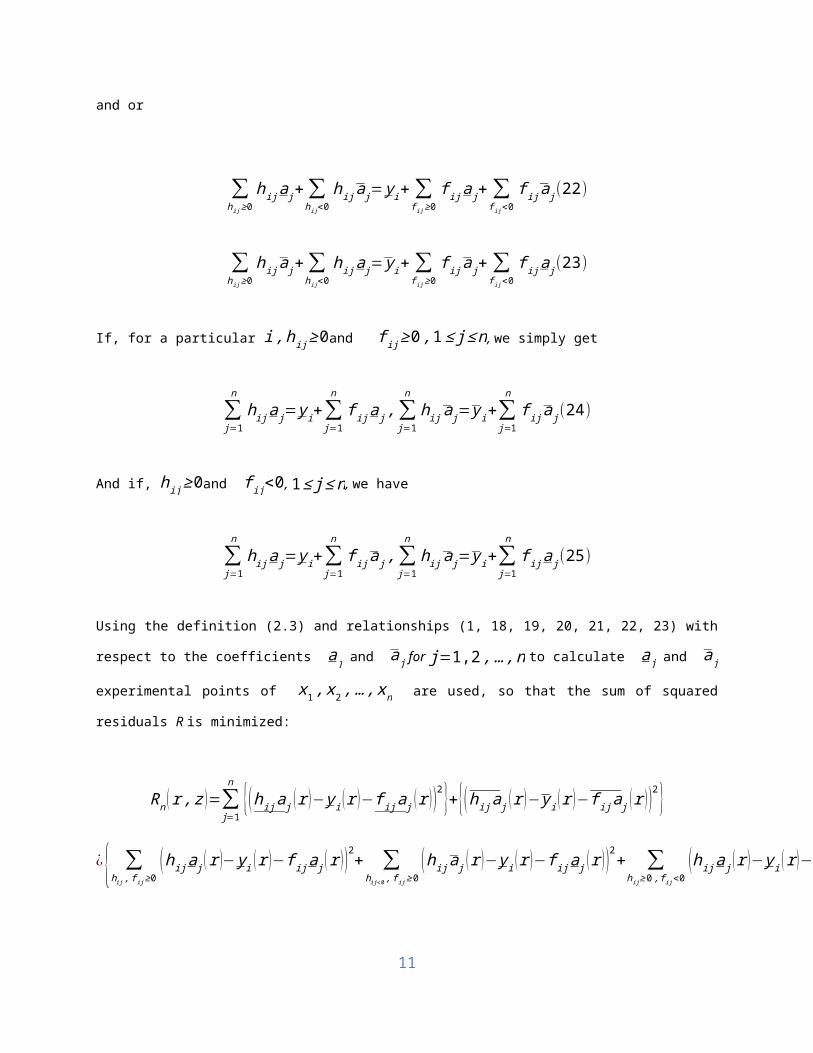
and or
∑hij ≥ 0
hij a j+∑hij<0
hij a j= y i+∑f ij≥ 0
f ij a j+∑f ij<0
f ij a j(22)
∑hij≥ 0
hij a j+∑hij<0
hij a j= y i+∑f ij≥ 0
f ij a j+∑f ij<0
f ij a j(23)
If, for a particular i ,h ij ≥ 0and f ij ≥ 0 ,1≤ j ≤n, we simply get
∑j=1
n
hij a j= yi+∑j=1
n
f ij a j ,∑j=1
n
hij a j= yi+∑j=1
n
f ij a j(24)
8

And if, hij ≥0and f ij<0, 1 ≤ j≤ n, we have
∑j=1
n
hij a j= y i+∑j=1
n
f ij a j ,∑j=1
n
hij a j= y i+∑j=1
n
f ij a j(25)
Using the definition (2.3) and relationships (1, 18, 19, 20, 21, 22, 23) with respect to the coefficients a j and a j for
j=1,2 ,…, n to calculate a j and a j experimental points of x1 , x2 , …, xn are used, so that the sum of squared
residuals R is minimized:
Rn (r , z )=∑j=1
n
{( hij a j (r )− yi (r )−f ij a j (r ) )2}+{(hij a j (r )− y i (r )−f ija j (r ))2}
¿ { ∑hij , f ij≥ 0
(hij a j (r )− y i (r )−f ij a j (r ) )2+ ∑hij<0 , f ij≥ 0
(hij a j (r )− y i (r )−f ij a j (r ) )2+ ∑hij ≥ 0 ,f ij<0
(hij a j (r )− y i (r )−f ij a j (r ) )2+ ∑hij , f ij<0
( hij a j (r )− y i (r )−f ij a j (r ) )2}+{ ∑hij ,f ij≥0
(hij a j (r )− y i (r )−f ij a j (r ))2+ ∑
hij<0 , f ij ≥0(hij a j (r )− y i (r )−f ij a j (r ) )2
+ ∑hij ≥0 , f ij<0
(hija j (r )− y i (r )−f ij a j (r ) )2+ ∑hij ,f ij<0
(hij a j (r )− y i (r )−f ij a j (r ))2}Wherez= {a1 (r ) , a2 (r ) ,…,an (r ) , a1 (r ) , a2 (r ) , …, an (r ) }. Thus the Fuzzy system (21) which is n-dimensional
transforms into 2n-dimensional real space. Finally, general constrained optimization problem is to find z so as to
minimize Rn
s . t(26)
a j (r )≤ a j (r ) , for j=1,2 ,…, n∧any rϵ [0,1]
all variables a j (r ) and a j (r ) are free:
Letz= {(a j (r ) , a j (r ) ) ,1≤ j ≤ n}denotes the unique solution of(22 or23),
then the fuzzy number vector V= {( v j (r ) , v j (r ) ) ,1≤ j≤ n , rϵ [0,1]}defined by
v j (r )=min {a j (α ) ,α ϵ [ r , 1 ] } , v j (r )=max {a j ( α ) , α ϵ [ r ,1 ] } is called the solution of(24). Then, for solving
FFIE by using ABC algorithm, position of nectar source is presented by the coordinate in 2n-dimensional real space.
It is the solution z of some special problem, and the quality of nectar source is presented by the objective function
R(r , z) of this problem. Accordingly, optimization of this problem is implemented by simulating behaviors of the
three kinds of bees. Thus, according to Section 4, for solving FFIE by using ABC method the following algorithm is
proposed.
Algorithm
9

1. Read the functions of FFIEs problem,
2. Set maximum cycle number (MCN),
3.Initialize the SN population of solutionsz i=(a1i , a2
i , …, ani , a1
i , a2i ,… , an
i) ,i=1,2 ,… , SN , (So that, at the
beginning of the ABC algorithm, SN numbers
of initial solutions (individuals) are randomly generated over the2ndimensional
problem space by using the following expression:
z ji=v j
i (r )+rand [ 0,1 ] × (v ji(r )−v j
i (r ) ) ,(27)
z ji=v j
i (r )++rand [ 0,1 ] × ( v ji(r )−v j
i (r ) ) .(28)
Which SN is the number of food sources iϵ {1,2 ,…, SN } and jϵ {1,2 , …, n } .Also, v ji ( r ) , v j
i (r ) are,
respectively, the lower and upper
limits of the jth optimization variable, and rand [ 0,1 ] denotes a uniformly distributed random number within [ 0,1 ]).
4. Evaluate the fitness value for each employed bee by using the following equation:
fit (r , z i )=fit (r )i=1
(1+Rn(r , z i)).(29)
In which that Rn (r , zi )is the value of the functional residual.
5. Set cycle number, cycle = 1,
6. Generate new solutions v i , v ifor the employed bees by following equation
and evaluate their fitness values.
v ji=z j
i (r )+∅ ji (z j
i−z jk ) ,
)30(
v ji=z j
i (r )+∅ ji (z j
i−z jk ) .
10
Wherei , kϵ {1,2 , …, SN } and jϵ {1,2, …, n } are randomly chosen indices, z jk is a randomly chosen solution
different from z ji ;∧v j
i , v jiis the new solution (food source). Also, ∅ j
i denotes a random number in the interval[-
1,1].
7. Apply the greedy selection process for z i and v ji , v j
i
8. Calculate the probability value pi corresponding to the solution z i by using.
pi=
fit (r )i
∑j=1
SN
fit (r ) j
(31)
9. Produce the new solutions v ji , v j
i for the onlooker bees from the old solutions z i selected depending on pi in
above equation and evaluate their fitness values.
10. Apply the greedy selection process between the old solution z i and new solution v ji , v j
i .
11. Determine the abandoned solution for the scout, if exists, and replace it with a new randomly produced solution
using (27, 28).
12. Memorize the best solution found so far.
13. Set cycle = cycle + 1and if cycle< MCN and R (r , zi )>ϵ go back to Step 6, and otherwise STOP.
6 Numerical example
In this section, we present three examples of linear Fredholm fuzzy integral equations and results will be compared
with the exact solutions.
Example 1: [39] Consider the following Fredholm integral equation (13) with:
y(x,r)=x3 ( r2+r ) , y(x,r)=x3 ( 4−r3−r ) (32)
and kernel
k ( x ,t )=x+1 ,−1 ≤ x , t ≤ 1and
a=−1 , b=1 , λ=1.The exact solution in this case is given by
~u=(x3 ( r2+r ) , x3 (4−r 3−r )).
11

let
h1 ( x )=1 , h2 ( x )=x3
and
x1=−1 , x2=1
With the implementation ABC algorithm (24), forr=0.25 , 0.5 ,0.75 we get
r ~a1~a2
0.25 (0,0) (0.3125,3.7344)
0.5 (0,0) (0.75,3.3750)
0.75 (0,0) (1.3125,2.8281)
Approximate solution and exact solution are compared in Fig1, Fig2 and Fig3.
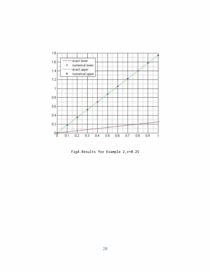
Example 2: [39] Consider the following Fredholm integral equation (13) with:
y(x,r)=r ( 12
x−13 ) , y(x,r)=(2−r)(1
2x−1
3 ), (33)
and kernel
k ( x ,t )=x+t ,0≤ x , t ≤ 1and
a=0 , b=1, λ=1.The exact solution in this case is given by
~u=(rx , (2−r ) x).
let
h1 ( x )=1 , h2 ( x )=x
and
x1=0 , x2=1
With the implementation ABC algorithm (24), for r=0.25 , 0.5 ,0.75 we get
12

r ~a1~a2
0.25 (0,0) (0.2499,1.7497)
0.5 (0,0) (0.4965,1.4983)
0.75 (0,0) (0.7501,1.25)
Approximate solution and exact solution are compared in Fig4, Fig5 and Fig6.
Example 3: [39] Consider the following Fredholm integral equation (13) with:
y(x,r) =−2π
cosx (r2+r) , y(x,r) =−2π
cosx(3−r ), (34)
and kernel
k ( x ,t )=cos (x−t) ,and
a=0 , b=2π
, λ= 4π
.
The exact solution in this case is given by
~u=((r2+r ) sinx , (3−r ) sinx).
let
h1 ( x )=x ,h2 ( x )=x3 ,h3 ( x )=x5
and
x1=0 , x2=π4
, x3=π3
, x2=π3−0.01 .
With the implementation ABC algorithm (24), for r=0.25 , 0.5 ,0.75 we get
r ~a1~a2
~a3
0.25 (0.3230, 2.8078) (-0.0938, -0.5511) (0.0173, 0.00485)
0.5 (0.7359, 2.5444) (-0.1046, -0.4335) (0.0009, 0.0213)
0.75 (1.3342, 2.2849) (-0.2639, -0.4551) (0.0227, 0.0415)
13

Approximate solution and exact solution are compared in Fig7, Fig8 and Fig9.
7 Conclusions
In this paper, Fredholm fuzzy integral equation of the second kind is solved by using optimization algorithm (ABC).
For some problems, the solution might not exist, and if it exists, solving problems may lead to a lot of difficulties.
For example, some methods have been proposed only for symmetric fuzzy functions, triangular fuzzy functions and
e.t.c. But our method do not have these constraints and this algorithm does not need to be continuous and derivative.
Also in this method, the volume of calculations are reduced. Such that, the integral equation in optimization model
and running algorithm (ABC) on it, we obtain a very good approximate solution. The numerical results obtained in
the examples show the effectiveness of the method.
Fig1.Results for Example 1,r=0.25
14

Fig2.Results for Example 1,r=0.5
Fig3.Results for Example 1,r=0.75
15

Fig4.Results for Example 2,r=0.25
16
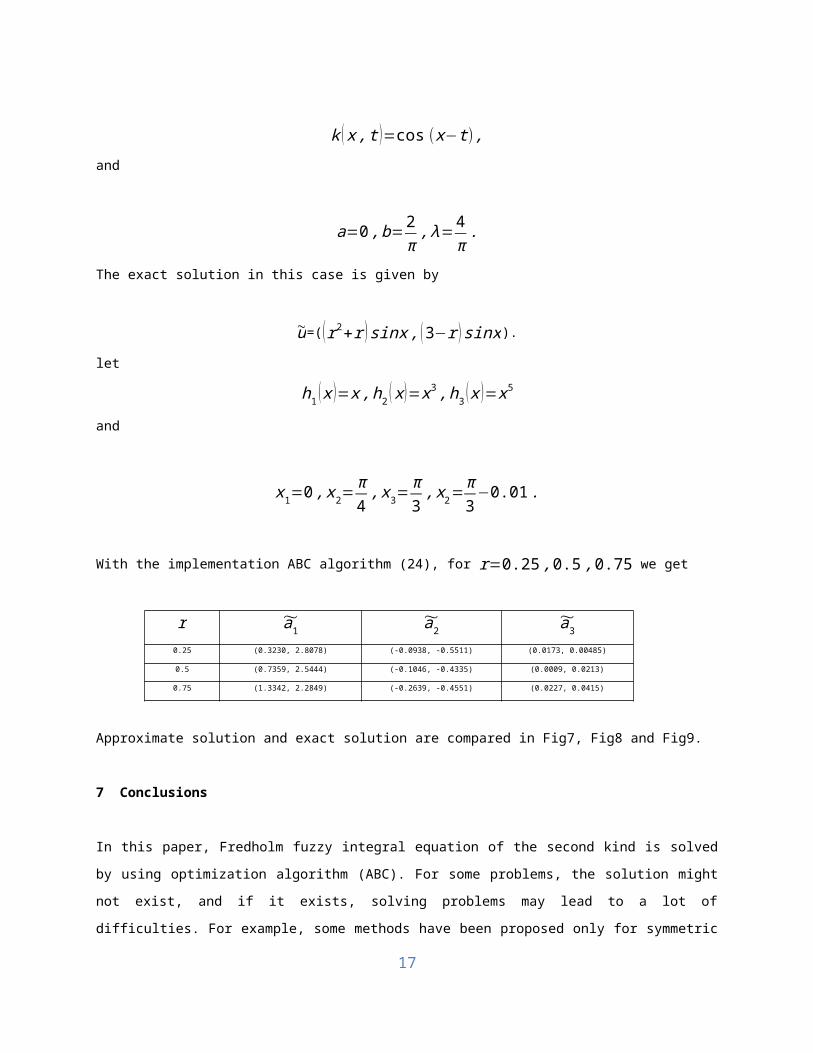
Fig5.Results for Example 2,r=0.5
Fig6.Results for Example 2,r=0.75
17

Fig7.Results for Example 3,r=0.25
Fig8.Results for Example 3,r=0.5
Fig9.Results for Example 3,r=0.75
18

References
[1] A. Alizadegan, B. Asady, M. Ahmadpour. Two modified versions of artificial bee colony algorithm, Applied
Mathematics and Computation.225 (2013) ,p.601-609.
[2] M. Alavi, B. Asady, Symmetric triangular and interval approximations of fuzzy solution to linear Fredholm
fuzzy integral equations of the second kind, Iranian Journal of Fuzzy Systems Vol. 9, No. 6, (2012) , p. 87-99.
[3] S. Abbasbandy, Numerical solution of integral equation: Homotopy perturbation method and Adomians
decomposition method, Appl. Math Comput. 173 (2006), p. 493-500.
[4] S.Abbasbandy, E. Babolian, M. Alavi, Numerical method for solving linear Fredholm fuzzy integral equations of
the second kind, Chaos Solitons Fraclals 31 (2007), p. 138-146.
[5] T. Allahviranloo and M. Otadi, Gaussian quadratures for approximate of fuzzy integrals, Applied Mathematics
and Computation, 170 (2005), p. 874-885.
[6] B. Asady, F. Hakimzadegan, R. Nazarlue, Utilizing artificial neural network approach for solving 3 two-
dimensional integral equations, Math Sic (2014) DOI 10.1007/s40096-014-0117-6.
[7] E. Babolian, H. Sadeghi Goghary, S. Abbasbandy, Numerical solution of linear Fredholm fuzzy integral
equations of thesecond kind by Adomian method, Appl. Math. Comput. 161 (2005), p. 33 - 44.
[8] E. Babolian, H. Sadeghi and S. Javadi, Numerically solution of fuzzy differential equations by Adomian
method, Appl. Math. Comput., 149 (2004), p. 547-557.
[9] K. Balachandran and K. Kanagarajan, Existence of solutions of general nonlinear fuzzy Voltera-Feredholm
integral equations, J. Appl. Math. Stochastic Anal, 3 (2005), p. 333-343.
[10] K. Balachandran and P. Prakash, Existence of solution of nonlinear fuzzy Voltera-Feredholm integral
equations, Indian J. Pure Appl. Math, 333 (2002), p. 329-343.
[11] B. Bede and S. G. Gal, Quadrature rules for integral of fuzzy-number valued functions, Fuzzy Sets and
Systems, 145 (2004), p. 359-380.
[12] A. M. Bica, Error estimation in the Approximation of the solution of nonlinear fuzzy Fered holm integral
equations, Information Sciences, 174 (2008), p. 1279-1292.
[13] L. C. Cagnina and S. C. Esquivel and C. A. C. Coello, Solving engineering optimization problems with the
simple constrained particle swarm optimizer, Informatica, (2008), p. 319-326.
[14] D. Dubois, H. prade, Operations on fuzzy numbers, J. Syst. Sci. 9 (1978) 613-626.
[15] M. Friedman, M. Ma, A. Kandel, Numerical methods for calculating the fuzzy integral, Fuzzy Sets Syst. 83
(1996), p. 57-62.
[16] R. Goetschel, W. Voxman. Elementary fuzzy calculus. Fuzzy Sets Syst. 18 (1986), p. 31-43.
[17] A. Kandel, Fuzzy statistics and forecast evaluation, IEEE Trans. Syst. Man Cybernet. 8 (1978), p. 396-401.
[18] O. Kaleva, Fuzzy differential equations, fuzzy sets and system, vol. 24, (1987), p. 301-317.
19
[19] J. Kennedy and R. Eberhart, Particle Swarm Optimization, Proceedings of IEEE International Conference on
Neural Networks IV. 4 (1995), p. 1942 – 1948.
[20] D. Karaboga, BahriyeAkay, A Comparative study of artificial Bee Colony Algorithm, Applied Mathematics
and Computation 214 (2009), p. 108-132.
[21] Karaboga, D.: An Idea Based on Honey Bee Swarm for Numerical Optimization, Erciyes University,
Engineering Faculty, Computer Science Department, Kayseri/ Turkiye, (2005).
[22] D. Karaboga, and B. Bastark, On the performance of artificial Bee Colony (ABC) Algorithm Journal of Soft
computing, vol. 8, (2008), p. 687- 697.
[23] D. Karaboga and B. Bastark, A Powerful and Efficient Algorithm for Numerical Function optimization:
artificial bee Colony (ABC) Algorithm. Journal of Global optimization, 39, (2007), p.459-471.
[24] D. Karaboga, BahriyeAkay, A Comparative study of artificial Bee Colony Algorithm Applied Mathematics and
Computation 214 (2009), p. 108-132.
[25] J. Kennedy and R. Eberhart, Particle Swarm Optimization, Proceedings of IEEE International Conference on
Neural Networks IV. pp.(1995).
[26] X. Lan, Variational iteration method for solving integral equations, Comput. Math.Appl. 54 (2007) , p. 1071-
1078.
[27] S. J. Liao, On the homotopy analysis method for nonlinear problems, Appl. Math. Comput.147 2004), p. 499-
513.
[28] S. J. Liao, Y. Tan, A general approach to obtain series solution of nonlinear differential equations, Stud. Appl.
math. 119 (2007), p. 297-355.
[29] M. Matloka, On fuzzy integrals, in proceeding 2nd polish symposium on interval and fuzzy Mathematics,
olitechnika poznansk, (1987), p. 167-170.
[30] M. Mizumoto, k. Tanaka. The four operations of arithmetic on fuzzy numbers, Syst. Comput. Controls 7 (5)
(1976), p. 73-81.
[31] P. Mansouri. B. Asady and N.Gupta. A Novel Iteration Method for solve Hard Problems( Nonlinear Equations)
with artifcial Bee Colony algorithm. World Academy of Science, Engineering and technology,
Vol. 59, (2011), p. 594-596, (2011).
[32] P. Mansouri, B. Asady, N.Gupta. An approximation algorithm for fuzzy polynomial interpolation with artifcial
Bee Colony algorithm. Applied Soft Computing. Vol.13, (2013), p. 1997-2002.
[33] P. Mansouri, B. Asady, N.Gupta, The Combination of Bisection Method and artificial Bee Colony Algorithm
for Solving Hard Fix Point Problems V. Snasel et al. (Eds.): SOCO Models in Industrial and Environmental Appl,
AISC 188, (2013), p. 33-41.
[34] P. Mansouri, B. Asady, N.Gupta, The Bisection-Artificial Bee Colony algorithm to solve Fixed point problems,
Applied Soft Computing, 2013; 13(4):1997-2002 DOI: 10.1016/j.asoc.2014.09.001.
[35] M. S. Osman, M. A. Abo-Sinna, A. A. Mousa, A solution to the optimal power flow using genetic algorithm,
Applied Mathematics and Commputation, Vol. 155, (2004), p.291-405.
20

[36] S. Sayah, K. Zehar, Modified differential evolution algorithm for optimal power flow with non- smooth cost
functions, Energy Conversion and Management, Vol. 49, (2008), p. 3036-3042.
[37] L.A. zadeh, Fuzzy sets, In form. Control 8 (1965), p. 338-353.
[38] X.S. Yang, Firey algorithms for multimodal optimization, Stochastic algorithms, foundations and applications,
Springer Berlin Heidelberg, (2009), p. 169-178.
[39] M.Jahantigh, T. Allahviranloo and M. Otadi, Numerical Solution of Fuzzy integral equations, Applied
Mathematical Sciences, Vol. 2, (2008), no. 1, p. 33-46.
21