view frustum culling and animated ray tracing
TRANSCRIPT

THESIS FOR THE DEGREE OFL ICENTIATE OF ENGINEERING
View Frustum Culling and Animated Ray Tracing:Improvements and Methodological
Considerations
ULF ASSARSSON
Department of Computer EngineeringCHALMERS UNIVERSITY OF TECHNOLOGY
Goteborg, Sweden 2001

View Frustum Culling and Animated Ray Tracing:Improvements and Methodological ConsiderationsULF ASSARSSON
Technical Report no. 396L
Department of Computer EngineeringChalmers University of TechnologySE–412 96 Goteborg, SwedenPhone: +46 (0)31–772 1000
Contact information:Ulf AssarssonABB Robotics Products ABDrakegatan 6SE–412 50 Goteborg, Sweden
Phone: +46 (0)31–773 8513Email: [email protected]: http://www.ce.chalmers.se/ ˜ uffe
Printed in SwedenChalmers ReproserviceGoteborg, Sweden 2001

View Frustum Culling andAnimated Ray Tracing: Improvements andMethodological ConsiderationsULF ASSARSSONDepartment of Computer Engineering, Chalmers University of Technology
Thesis for the degree of Licentiate of Engineering, a Swedish degreebetween M.Sc. and Ph.D.
Abstract
Today’s algorithms and computers are orders of magnitude too slow for photo-realisticrendering of complex scenes in real time. Even though the speed of graphics render-ing hardware grows rapidly, there are strong reasons to believe that we will never getsufficient rendering power for naive algorithms. Algorithmic performance improvingtechniques are therefore essential.
This thesis presents new performance improving techniques, as well as tools andmethodologies to be used in research aimed at performance improving algorithms. Fournew algorithmic improvements for fast culling of objects that are outside the field-of-view (view frustum culling) are evaluated in combination with existing methods. Theexecution times are measured and compared between the implementations. The re-sults show that the new techniques are successful in lowering the amount of work thatneeds to be done. Furthermore, different combinations of improvements are evaluated.The thesis also investigates how to utilize multiprocessors to speed up view frustumculling compared to using only one processor. A number of previously documentedload distribution schemes are implemented and the amount of resulting parallelism isevaluated. The results show that the communication cost (communication/computationratio) involved in the load distribution is too high for the schemes to provide signif-icant speedup. However, with a number of straightforward tricks that are presented,this is circumvented, and a speedup of four is achieved on eight processors. With thesame load distribution scheme applied on collision detection, the speedup is three timeson seven processors. Finally, the thesis presents a benchmark and a methodology forcomparing algorithms for animated ray tracing. The criteria for comparing ray tracingalgorithms are identified. The potential stresses of existing ray tracing algorithms arecategorized. The result is a benchmark, implementing the stresses into three scenes,and a methodology for comparing algorithms where image quality may be traded forspeed.
Keywords: View frustum culling, parallel tree traversal, collision detection, animatedraytracing, bench-mark, 3D computer graphics.
i

ii
List of Appended Papers
The thesis is a summary of the following papers. References to the papers will be madeusing the Roman numbers associated with the papers.
I . Ulf Assarsson and Tomas Moller, “Optimized View Frustum Culling Algorithmsfor Bounding Boxes,”Journal of Graphics Tools, 5(1), Pages 9-22, 2000. Cor-responding tech-report:“Optimized View Frustum Culling Algorithms,”Techni-cal Report 99-3, Department of Computer Engineering, Chalmers University ofTechnology, http://www.ce.chalmers.se/staff/uffe/, March 1999.
II . Ulf Assarsson and Per Stenstrom,”A Case Study of Load Distribution in ParallelView Frustum Culling and Collision Detection,”Department of Computer Engi-neering, Chalmers University of Technology, Sweden, January 2001. Submittedfor publication.
III . Ulf Assarsson, Jonas Lext and Tomas Moller, ”BART: A Benchmark for Ani-mated Ray Tracing,”IEEE Computer Graphics and Applications, Pages 22-30,March/April, 2001.
iii

iv

1 Introduction
Computer graphics is the science of how to generate (render) images with computers.This includes algorithms for creating realistic images of three dimensional scenes byusing geometrical models and shading models. One particular goal is to achieve theimage quality of a photograph or even images that are indistinguishable from the reality.In real time computer graphics, the images should be updated fast enough to give theimpression of smooth motions, such as that used in TV. The problem is that today’salgorithms and computers are orders of magnitude too slow to be able to generate photo-realistic images in real time. Therefore, performance improvement techniques to makegraphics algorithms run faster are important. This thesis considers two applications:view frustum culling and animated ray tracing.
A three dimensional scene is typically composed of several individual objects (like atable, a sofa, chairs etc) represented by geometry. Triangles are often used as a primitiveto approximately catch the shape, since they can be rendered fast by graphics hardware.Upon traditional rendering, the objects are usually drawn to the image one by one,triangle by triangle, as seen from the desired view-point. Objects outside the field-of-view do not affect the result of the image (except if they cast shadows into the imageor are reflected by visible objects - but that is usually handled separately), and thusneed not be rendered. View frustum culling (VFC) is the technique for determiningwhether or not an object currently is located within the field-of-view and discardingobjects outside.
Ray tracing is an alternative method to rendering objects one by one for generatingimages [12, 13]. Virtual rays of light are traced, typically backwards from the viewer’seye into the scene, in order to determine the color of each picture element (pixel). Ray-tracing is typically slower than hardware accelerated triangle rendering, but is able tocreate very realistic images with simple and general algorithms, and is therefore verypopular. With the improvements of computer performance and algorithms, it is nowpossible to ray trace simple scenes in real time. However, there is an absence of a wayto compare the performance of algorithms for animated ray tracing, i.e., ray tracing ofscenes where objects are moving.
This thesis considers performance improvement techniques for view frustum cullingand a methodology for comparing the performance of algorithms for animated ray trac-ing. The thesis is a summary of three papers, denoted with Roman numeralsI , II andIII . The contribution ofI is new algorithm improvements and evaluation of combina-tions of improvements for view frustum culling. The contribution ofII is a case studyof parallel view frustum culling focused on how to utilize multiple processors to getsignificant speedup. In particular, we evaluate the usefulness of previously publishedload distribution strategies. The contribution ofIII is a methodology for evaluating raytracing algorithms for animated scenes. It is also a set of rules on how to measure andcompare rendering performance and image quality.
The thesis commences with explanations of the problems and contributions for each
1

paper. The papers on view frustum culling (I andII ) are treated in Section 2. Comparingperformance of algorithms for animated ray tracing (III ) is summarized in Section 3.
2 View Frustum Culling
The view frustum is the pyramid-shaped volume in front of the viewer within the field-of-view, and with the eye at the top. The four planes defining the sides of the pyramidvirtually passes through the window borders. Usually a near plane and far plane isadded [4], cutting the top off the pyramid and limiting the depth. In this case the viewfrustum is totally defined by 6 planes (see Figure 1).
Figure 1: The view frustum is the area in grey in front of the eye or the camera. It isdefined by the window extensions, the field-of-view, and the near- and far planes.
View frustum culling is a technique for determining which objects that are outsidethe view frustum. Objects outside the view frustum are not visible (possibly with theexception of reflections) and thus are unnecessary to render.
For each object a bounding volume is computed that is faster to test against thefrustum than the object itself. The bounding volume (BV) should enclose the objectcompletely, and at the same time be as tight-fitting as possible. Bounding spheres andbounding boxes are two popular entities. A test is devised such that the intersectionbetween the BV and the six planes can be determined. The BV is tested geometricallyagainst the six planes of the frustum. If the BV is inside all six planes, the object istotally inside the view frustum and should be rendererd. If the BV is outside at leastone of the planes, the object is totally outside the frustum and does not need to berendered. Otherwise, the object is sent for rendering since it may be visible.
View frustum culling is often performed hierarchically, to avoid testing each indi-vidual object against the view frustum. Sometimes the scene’s natural hierarchy is used,and sometimes a separate BV hierarchy is created. A BV hierarchy may be created inthe following way. Objects close to each other are clustered into groups and for each re-sulting group, a bounding volume is computed, enclosing all its members BVs. Nearbygroups are then clustered into larger groups, with their BVs computed equally, and soon until there is only one BV enclosing the whole scene. The hierarchy is representedas a tree structure. A natural structure could for instance be a root node representing a
2

room with one of the child nodes representing a table in the room, and with its childrenrepresenting the four legs and the board.
When rendering the scene, the BV-tree is traversed top-down, and for each nodethe bounding volume is tested for intersection with the view frustum. If the boundingvolume is totally inside the frustum, the contents of the subgraph is marked for render-ing. If it is totally outside, the subgraph is pruned. Otherwise, the traversal continuesrecursively.
A framerate of 70-85 frames per second (fps) is sufficient for smooth motions [8,10]. This gives 12-13 milliseconds of computation time for each frame. If there aremany objects that need to be tested, for instance in a large scene, the VFC may requirea major part of this time. It is important to free CPU time for all other necessary tasks,such as animation, application logic, artificial intelligence etc. Thus it is important toimprove the VFC algorithm for speed.
2.1 Optimized View Frustum Culling Algorithms
In some disciplines,optimizationis often loosely meant as an improvement, in terms ofexecution time, of some algorithms. In this section we use optimization in that sense.
PaperI presents three new optimizations –the plane-coherency test, the octant test,and the Translation and Rotation coherency test (TR test)– and analyzes their effi-ciency. All presented techniques here involve adding computations in one step, assum-ing this can save computations in another step. The circumstances under which theoptimizations are efficient sometimes overlap, and thusI also evaluates how to bestcombine the new and existing optimizations in order to maximize performance. In thispaper only the most promising combinations are presented. In a corresponding techni-cal report [2] more detailed results are reported.
The plane coherency test utilizes temporal coherence. An object that was outside aplane during the previous frame is likely still outside that plane during the next frame,and thus by testing against that plane first, testing of the other planes can often beavoided. The TR test uses previous results and considers the change in viewer positionto determine which objects that must remain inside or outside the frustum.
The octant test exploits the fact that it is sufficient to test the BV against the threeclosest planes of a symmetric frustum.
The VFC algorithm used as a base for the added optimizations is derived fromthe idea that the problem can be transformed into testing one point against a sweptvolume [3]. For bounding boxes this results in an algorithm presented by Green [6].This algorithm, in itself and together with different combinations of optimizations, iscompared against another popular method where the BV is transformed into frustumspace (perspective coordinate system) and surrounded by a new axis-aligned boundingbox. In this system the frustum is also an axis-aligned bounding box and the resultingtwo bounding boxes are compared against each other.
The tests were performed on a personal computer using three industrial models as
3

environments. Since the speedup of the algorithms are highly dependent of the 3D-environment, position of the viewer, and how the viewer is moved, four different pathsfor the viewer for each scene were used.
The results show that the plane coherency test should always be used, and preferablyin combination with either the octant test or the TR test or both. The TR coherencyoptimization was especially fruitful when the navigation involves either pure rotation orpure translation and gave up to a ten-fold speedup. In this case the plane coherency testplus the TR test combination gave the best performance. For other types of navigationthe plane coherency test plus the octant test combination was preferable.
2.2 Parallel View Frustum Culling and Collision Detection
Hierarchical VFC of complex scenes with large BV-trees requires high computing per-formance if a high frame rate should be achieved. Using multiprocessor systems is oneway to increase the available computing power. The work load must be balanced be-tween the processors in order to utilize the system efficiently. Load distribution cannotbe done statically (once for all frames) since the actual work, i.e., the traversed andtested BVs, varies between different frames as the viewer or objects move.
The difficulty in a load distribution scheme for view frustum culling is that the com-putation cost at each node is very small (at the size of hundreds of cycles). In our targetmultiprocessor systems, the approximate time for the inter-processor communicationcost is 100 clock cycles. This means that the penalty of communication is very high andthat it is important to avoid all unnecessary communication, such as communication forsynchronization of the sending and receiving processors. The cost of distributing workto another (typically less loaded) processor must be lower than the cost of performingthe work itself, in order to benefit from dynamic load balancing.
A comparative evaluation of several previously documented load distribution strate-gies is presented inII in order to determine if they are suitable for parallel hierar-chical VFC algorithms. There are lots of previous research on parallel tree traver-sals [9, 14, 15], but none has explicitly considered VFC. The kind of work done at eachnode strongly affects the characteristics of the parallel tree traversal, like cache-missbehavior and load-balance. Thus it is important to make an investigation particularlyfor view frustum culling.
The same three industrial models used inI were used as test scenes – all highlyunbalanced. Balanced scenes would be easier to traverse in parallel, but such scenescannot be expected by a real visual application. The camera was moved along onespecific path – sampled from user navigation – for each model, involving both rotationand translation between many frames. The VFC algorithm utilizes the plane-coherencytest and the octant test as this was one of the best combinations of optimizations fromI .
The algorithms were implemented on a Sun Enterprise 4000 shared-memory mul-tiprocessor system. This machine is equipped with 14 UltraSPARC-II CPUs running
4

at 248 MHz. The execution times of the parallel experiments were measured and com-pared with the execution times of the algorithms when run on only one processor.
The evaluated previously documented load distribution schemes were found inca-pable of providing meaningful speedup when using multiple processors compared tousing one processor. PaperII presents a modified scheme for which no synchronizationis required when load balancing. On many multiprocessor systems all communicationis performed at the so-called cache-block level, i.e., a whole block of data (typically32 bytes) is sent in just a little bit more time it would take to send just one byte. Thescheme utilizes this to lower the average distribution cost of a job to further reduce thecommunication cost. With the proposed scheme, up to about a four-fold speedup oneight processors was achieved.
As a final contribution, the success of the suggested load distribution scheme ap-plied on collision detection is tested. Collision detection is a problem instance similarto VFC, where the BV-trees of two objects are tested mutually for intersection. Aspeedup of three times was achieved for seven processors.
PaperII shows that it is possible to get significant speedups with parallel VFC andcollision detection in real applications, if a suitable load distribution strategy is used.
3 BART: A Benchmark for Animated Ray Tracing
Ray tracing is an alternative to rendering objects one by one for creating images. Typi-cally it is slower but able to generate images of higher quality. Relatively simple algo-rithms are capable of rendering phenomena such as shadows and reflections.
For each picture element (pixel) of an image, a virtual ray of light is traced into thescene in order to find the closest hit object (the visible object at that spot). Accelerationdata structures, built from the scene data, are commonly used to speed up this process.It could for instance be a BV hierarchy, where only the members of BVs penetrated bythe ray, are searched.
For static scenes, the acceleration structures are usually built in a preprocessingstep. For an animated scene, the data structures have to be rebuilt or updated betweensuccessive frames.
In the last few years real-time ray tracing has become a reality due to faster pro-cessors and improved algorithms, but still only fairly simple scenes can be rendered.When striving for ray tracing algorithms with higher performance and to help pushingresearch, it is essential to be able to compare the performance of different algorithms.
The goal of paperIII is to identify the important criteria when comparing algo-rithms for animated ray tracing and implement a benchmark based on the results. Thebenchmark must consider features that stresses the algorithms. It also needs to specifya methodology for comparing the performance of the rendering. Since it is common totrade image quality for speed by using approximations it is also necessary to be able tomeasure and compare the differences in image quality due to approximation errors.
5

A number of benchmarks and test scenes for image rendering exist [1, 5, 7, 11], butnone of them is appropriate for comparing algorithms of animated ray tracing.
The circumstances that tend to stress existing ray tracing algorithms, i.e., loweringthe speed, were identified and categorized into eight groups. All eight types of stresseswere implemented into the benchmark in three test scenes –kitchen, robots, andmu-seum.
The benchmark can be used in two modes:predeterminedandinteractivemode. Inpredetermined mode it is allowed to utilize information about the future, i.e., how theobjects and camera are going to move in the following frames. In interactive mode thisis prohibited to simulate a non-predictable future, for example if a viewer is navigatingin real time and objects are moved unpredictably by for instance artificial intelligencealgorithms.
The following types of potential stresses were identified: 1)Hierarchical animationusing translation, rotation and scaling. An animated object may have a tree structure(for instance a BV-tree), where nodes within the tree are animated and requires the ac-celeration structure to be updated between frames. This costs computation time. 2)Unorganized animation of objects, like waves on a surface or a squeezed ball, alsorequires the data structure to be updated. 3)”Teapot in the stadium” problem. Thedistribution of objects or details is highly unbalanced, which severely lowers the effi-ciency of certain acceleration structures. 4)Low frame-to-frame coherency. Some raytracing algorithms utilizes similarities between adjacent frames. 5)Large working sets.Reading data from the main memory is typically slow. If scenes are used that do notfit into the memory caches of the processor(s), this may induce overhead. 6)Boundingvolume overlap. It is common to test a ray for intersection of the bounding volume ofseveral objects/entities before testing the ray against each internal element. If a ray pen-etrates several overlapping BVs, all the members of those BVs have to be tested, whichincreases the amount of work that has to be done. 7)Changing object distribution.The acceleration structure that is most efficient often varies with the object distribution.When the object distribution changes, the chosen acceleration structure may becomeinappropriate. Computing a new acceleration structure costs CPU time. 8)The numberof light sourcesoften affects the rendering time of ray tracing algorithms. The morelight sources, the more work needs to be done to consider shadows correctly.
It is desirable to be able to compare different algorithms implemented by differentresearchers on different computers. To do this objectively, paperIII suggests that anumber of parameters and measures should be presented, of which some are: imageresolution, number of frames the animation is divided into, processor speed, availablememory, total rendering time, average frame time, worst frame time, preprocessingtime. Moreover, a graph showing the rendering time as a function of the frame numbershould be presented.
Hopefully, the benchmark will be used extensively in future research, and evolveover time.
The authors of paperIII have equally contributed to the work described here.
6

Acknowledgements
My first thanks go to my supervisor Professor Per Stenstrom for guiding me and teach-ing me how to be a good Ph.D student and perform quality research.
Tomas Moller deserves a whole page of thanks. He was the one that opened thedoor for me into the world of computer graphics research. He made me realize it ispossible to do Ph.D studies in this interesting field. He found the perfect professor –Per Stenstrom – and also gave me an excellent start with his idea of writing a VFC-paper together. I look forward to many further exiting and mind thrilling projects andpapers together in the future.
I want to thank Jonas Lext for inspiring discussions, exchange of ideas and for beinga great fellow traveller to conferences. A special thanks to Jonas and Henrik Holmdahlfor suggesting interesting courses and forcing me to read them. Thank you Bjorn An-dersson for interesting discussions of computer science and graphics algorithms, andthanks to all the nice people at the institution.
Several co-workers at ABB deserve mentioning. Acknowledgement to Nabbe, Pafvel,Johannes, Robert, Anders, Daniel, Carina for great gaming of 3D intensive creations,to Gregers for spreading information, and to the Henriks.
Finally I also want to thank ABB Robotics Product AB for the financial support.
7

References
[1] 3DMark,http://www.madonion.com/entry.shtml
[2] Ulf Assarsson and Tomas Moller, “Optimized View FrustumCulling Algorithms,” Technical Report 99-3, Department ofComputer Engineering, Chalmers University of Technology,http://www.ce.chalmers.se/staff/uffe/, March 1999.
[3] M. de berg, M. van Kreveld, M. Overmars, O. Schwarzkopf,“Compu-tational Geometry – Algorithms and Applications,”Springer-Verlag,Berlin, 1997.
[4] James D. Foley, Andries Van Dam, Steven K. Feiner, John F.Hughes, ”Computer Graphics Principles and Practice,”Addison-Wesley, ISBN 0-201-84840-6, pages 229-235.
[5] The Graphics Performance Characterization Group,http://www.specbench.org/gpc/ .
[6] Daniel Green, Don Hatch, “Fast Polygon-Cube Intersection Testing”,Graphics Gems V, Heckbert, pp. 375–379, 1995.
[7] Haines, Eric, “A Proposal for Standard Graphics Environments,”IEEEComputer Graphics and Applications, vol. 7, no. 11, pages 3–5,November 1987.
[8] James L. Helman, ”Architecture and Performance of EntertainmentSystems, Appendix A,”ACM SIGGRAPH 94 Course Notes – Design-ing Real-Time Graphics for Entertainment, vol 23, pages 1.19 – 1.32,July, 1994
[9] V. Nageshwara Rao and Vipin Kumar, ”Parallel Depth-First Searchon Multiprocessors — Part I: Implementation; and Part II—analysis”,International Journal of Parallel Programming, vol. 16, no. 6, 1987.
[10] Tomas Moller and Eric Haines,”Real-Time Rendering,”A.K. PetersLtd., ISBN 1-56881-101-2, p 1.
[11] Peter Shirley,http://www.radsite.lbl.gov/mgf/scenes.html.
[12] Peter Shirley, ”Realistic Ray Tracing,” A K Peters Ltd, ISBN:1568811101, June 2000.
[13] Turner Whitted, ”An Improved Illumination Model for Shaded Dis-play,” Communications of the ACM, 23 (6), pp. 343-349, June 1980.
8

[14] C. Xu, S. Tschoke, and B. Monien, ”Performance Evaluation of LoadDistribution Strategies in Parallel Branch and bound Computations”,Proc. of the 7th IEEE Symposium of Parallel and Distributed Process-ing (SPDP95), Oct. 1995.
[15] Myung K. Yang, Chita R. Das, ”Evaluation of a Parallel Branch-and-Bound Algorithm on a Class of Multiprocessors”,IEEE Transactionson Parallel and Distributed Systems, vol. 5, no. 1, January, 1994.
9

Paper I
Optimized View Frustum Culling Algorithms forBounding Boxes
Reprinted from
Journal of Graphics Tools, 5(1), Pages 9-22, 2000.


Optimized View Frustum CullingAlgorithms for Bounding Boxes
Ulf Assarsson and Tomas M¨oller
Department of Computer Engineering
Chalmers University of Technology, Sweden
Accepted for publication injournals of graphics tools
March 1999, revised February 2000
Abstract
This paper presents optimizations for faster view frustum culling (VFC) for axis aligned bounding box(AABB) and oriented bounding box (OBB) hierarchies. We exploit frame-to-frame coherency by caching andby comparing against previous distances and rotation angles. By using an octant test, we potentially halve thenumber of plane tests needed, and we also evaluate masking, which is a well-known technique. The optimizationscan be used for arbitrary bounding volumes, but we only present results for AABBs and OBBs. In particular, weprovide solutions which is2 � 11 times faster than other VFC algorithms for AABBs and OBBs, depending onthe circumstances.
1 Introduction
Bounding volume hierarchies are commonly used to speed up the rendering of a scene by using a view frustumculling (VFC) algorithm on the hierarchy [Clark76]. Each node in the hierarchy has a bounding volume (BV)that encloses a part of the scene. The hierarchy is traversed from the root, and if a BV is found to be outsidethe frustum during the traversal, then the contents of that BV need not be processed further, and performance isgained. Reducing the time for view frustum culling will increase performance of a single processor system andfree processor time to other tasks. With view frustum culling taking 6 ms before speedup and 1.2 ms after speedup1
and with 33 frames per second (30 ms/frame, no synchronization to monitor frequency), the view frustum cullinggoes from taking20% of total execution time to only4%, thus saving16%.
We present several optimizations for culling axis-aligned bounding boxes (AABBs) and oriented boundingboxes (OBBs) against a frustum used for perspective viewing. Frame-to-frame coherency is exploited by cachingand by comparing against previous distances and rotation angles. An octant test is introduced, which potentiallyhalves the number of plane tests needed, and we also evaluate masking [Bishop98]. All these optimizations canbe used for arbitrary bounding volumes which we show in our technical report [Assarsson99], where we alsoinvestigate bounding spheres, with speedups2 from 1:2 up to1:4 times. That report also provides more details onthe results for AABBs.
2 Related Work
When reviewing existing view frustum culling algorithms [Bishop98, DirectModel, Hoff96a, Hoff96b, Hoff97,Green95, Greene94], we found that there are two common ways to approach the view frustum culling problem.
1These are our figures for path 1, model 3 with the plane-coherency and octant test optimization (see section 4).2In this paper we define speedup astime1/time2, which means that a speedup of 1.0 is no speedup at all.
1
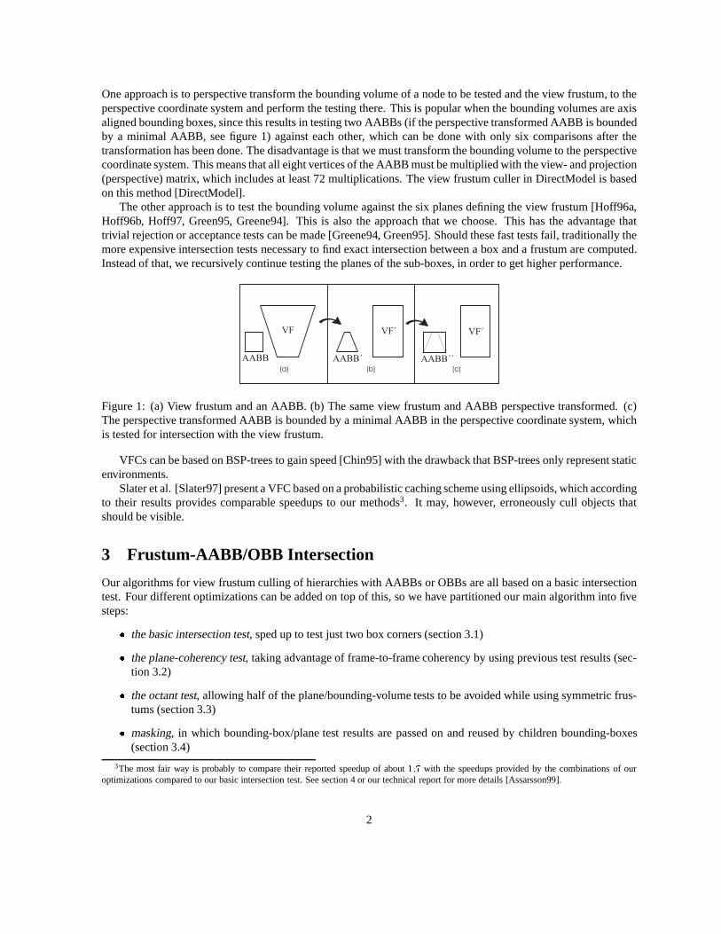
One approach is to perspective transform the bounding volume of a node to be tested and the view frustum, to theperspective coordinate system and perform the testing there. This is popular when the bounding volumes are axisaligned bounding boxes, since this results in testing two AABBs (if the perspective transformed AABB is boundedby a minimal AABB, see figure 1) against each other, which can be done with only six comparisons after thetransformation has been done. The disadvantage is that we must transform the bounding volume to the perspectivecoordinate system. This means that all eight vertices of the AABB must be multiplied with the view- and projection(perspective) matrix, which includes at least 72 multiplications. The view frustum culler in DirectModel is basedon this method [DirectModel].
The other approach is to test the bounding volume against the six planes defining the view frustum [Hoff96a,Hoff96b, Hoff97, Green95, Greene94]. This is also the approach that we choose. This has the advantage thattrivial rejection or acceptance tests can be made [Greene94, Green95]. Should these fast tests fail, traditionally themore expensive intersection tests necessary to find exact intersection between a box and a frustum are computed.Instead of that, we recursively continue testing the planes of the sub-boxes, in order to get higher performance.
Figure 1: (a) View frustum and an AABB. (b) The same view frustum and AABB perspective transformed. (c)The perspective transformed AABB is bounded by a minimal AABB in the perspective coordinate system, whichis tested for intersection with the view frustum.
VFCs can be based on BSP-trees to gain speed [Chin95] with the drawback that BSP-trees only represent staticenvironments.
Slater et al. [Slater97] present a VFC based on a probabilistic caching scheme using ellipsoids, which accordingto their results provides comparable speedups to our methods3. It may, however, erroneously cull objects thatshould be visible.
3 Frustum-AABB/OBB Intersection
Our algorithms for view frustum culling of hierarchies with AABBs or OBBs are all based on a basic intersectiontest. Four different optimizations can be added on top of this, so we have partitioned our main algorithm into fivesteps:
� the basic intersection test, sped up to test just two box corners (section 3.1)
� the plane-coherency test, taking advantage of frame-to-frame coherency by using previous test results (sec-tion 3.2)
� the octant test, allowing half of the plane/bounding-volume tests to be avoided while using symmetric frus-tums (section 3.3)
� masking, in which bounding-box/plane test results are passed on and reused by children bounding-boxes(section 3.4)
3The most fair way is probably to compare their reported speedup of about1:7 with the speedups provided by the combinations of ouroptimizations compared to our basic intersection test. See section 4 or our technical report for more details [Assarsson99].
2
� TR4 coherency test, which allows reuse of previous frame test results when the view changes in limited ways(section 3.5)
The optimizations can be utilized in a VFC independently of each other. That is, we can choose and combine thesteps anyway we like. A view frustum (VF) is defined by six planes:
�i : ni � x+ di = 0 (1)
i = 0 : : : 5, whereni is the normal anddi is the offset of plane�i, andx is an arbitrary point on the plane. We saythat a pointx is outside a plane�i if ni � x + di > 0. If the point is inside all planes then the point is inside theview frustum.
3.1 Basic Intersection Test
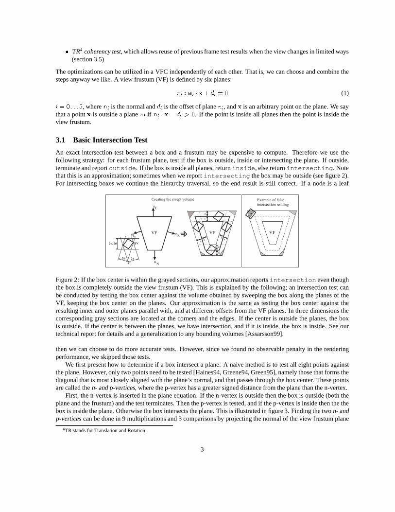
An exact intersection test between a box and a frustum may be expensive to compute. Therefore we use thefollowing strategy: for each frustum plane, test if the box is outside, inside or intersecting the plane. If outside,terminate and reportoutside . If the box is inside all planes, returninside , else returnintersecting . Notethat this is an approximation; sometimes when we reportintersecting the box may be outside (see figure 2).For intersecting boxes we continue the hierarchy traversal, so the end result is still correct. If a node is a leaf
BV
2a2b
2c, 2d
Creating the swept volume Example of false
intersection reading
Figure 2: If the box center is within the grayed sections, our approximation reportsintersection even thoughthe box is completely outside the view frustum (VF). This is explained by the following; an intersection test canbe conducted by testing the box center against the volume obtained by sweeping the box along the planes of theVF, keeping the box center on the planes. Our approximation is the same as testing the box center against theresulting inner and outer planes parallel with, and at different offsets from the VF planes. In three dimensions thecorresponding gray sections are located at the corners and the edges. If the center is outside the planes, the boxis outside. If the center is between the planes, we have intersection, and if it is inside, the box is inside. See ourtechnical report for details and a generalization to any bounding volumes [Assarsson99].
then we can choose to do more accurate tests. However, since we found no observable penalty in the renderingperformance, we skipped those tests.
We first present how to determine if a box intersect a plane. A naive method is to test all eight points againstthe plane. However, only two points need to be tested [Haines94, Greene94, Green95], namely those that forms thediagonal that is most closely aligned with the plane’s normal, and that passes through the box center. These pointsare called then- and p-vertices, where the p-vertex has a greater signed distance from the plane than the n-vertex.
First, the n-vertex is inserted in the plane equation. If the n-vertex is outside then the box is outside (both theplane and the frustum) and the test terminates. Then the p-vertex is tested, and if the p-vertex is inside then the thebox is inside the plane. Otherwise the box intersects the plane. This is illustrated in figure 3. Finding the twon- andp-verticescan be done in 9 multiplications and 3 comparisons by projecting the normal of the view frustum plane
4TR stands for Translation and Rotation
3

plane
Figure 3: The negative far point (n-vertex) and positive far point (p-vertex) of a bounding box corresponding toplane� and its normal.
bool intersect = false
for i in [all view frustum planes �i] dovn negative far point ( n-vertex ) in world
coordinates of box relative to �ia vn � ni + diif a > 0 then return Outsidevp positive far point ( p-vertex ) in world
coordinates of box relative to �ib vp � ni + diif b > 0 then intersect = true
end loopif intersect then return Intersectingelse return Inside
Figure 4: Pseudo code of general algorithm for culling AABBs or OBBs
on to the box’s axes and test the signs of the x-, y- and z-components of the projection. Since all AABBs are givenin the world coordinate system (aligned to the world x-, y- and z-axes) and we transform all view frustum planeequations (i.e. plane normals and offsets) to world coordinates at the beginning of each frame, we have the AABBsand the normal of the planes in the same coordinate system, which makes a projection unnecessary. We can usethe signs of the x-, y- and z-components of the plane normal immediately, leaving us with only three comparisons.If we create a bitfield of the signs, letting for instance a negative sign be represented by a ’0’ and a positive signbe represented by a ’1’, we can use this bitfield to get the p-vertex from a Look Up Table (LUT). In this way weavoid the conditional branches caused by if-statements, which can lead to expensive processor pipeline predictionmisses. This idea is used by Donovan et al. to accelerate clipping [Donovan94]. If we order the LUT properly, wecan invert the bitfield to get the n-vertex.
If we are going to test multiple AABBs against the view frustum (which generally is the case) and since allAABBs have the same orientation, it is a good idea to precompute the bitfields (indices to the n- and p-vertices)for each view frustum plane once each frame [Haines94].
A listing of the algorithm for testing a box against a frustum is given in figure 4.
3.2 The Plane-Coherency Test
The goal of this test is to exploit temporal coherence. Assume that a BV of a node was outside one of the viewfrustum planes last time it was tested for intersection (previous frame). For small movements of the view frustumthere is a high probability that the node is outside the same plane this time, which means that we should start testing
4

against that plane hoping for fast rejection of the BV. If the BV was outside a plane last frame, then an index tothis plane is cached in the BV structure. For each intersection test, we start testing against that plane and test theothers afterwards if necessary.
We test the planes in the order:left, right, near, far, up, anddown. No experiments in finding an “optimal”order has been conducted.
3.3 The Octant Test
Assume that we split the view frustum in half along each axes, resulting in eight parts, like the first subdivision ofan octree. We call each part anoctantof the view frustum.
Figure 5: (a) 2D-view of a symmetric view frustum divided in half along each axis.�a and�b are the outer planesof octantO. �c and�d are the inner planes. (b) View frustum divided in octants. (c) For a symmetrical VF itis sufficent to test for intersection against the outer planes of the octant in which the center (cS) of the boundingsphere (of the box) lies.
If we have a symmetrical view frustum, which is the most common case (a CAVE [CrusNeira93] is one excep-tion), and a bounding sphere, it is sufficient to test for culling against the outer three planes of the octant in whichthe center of the bounding sphere lies (see figure 5). This means that if the bounding sphere is inside the threenearest (outer) planes, it must also be inside all planes of the view frustum. If it is outside any of the planes, weknow it is totally outside the view frustum, and otherwise it is intersecting.
This can be extended to general bounding volumes; see our report [Assarsson99]. To be able to use the octanttest for boxes, the distance from the box center to a box corner must be smaller than the smallest distance fromthe view frustum center5 to the frustum planes (see figure 6). This is true, since an arbitrary BV cannot intersectthe planes of another octant without intersecting the planes of the selected octant, if the above holds. The distancebetween the center of the view frustum and its nearest plane can be precomputed once for each frame.
The cost of locating the octant was found to be approximately equal to one plane/box test.
3.4 Masking
Assume that a node’s BV is completely inside one of the planes of the view frustum. Then, as pointed out byBishop et al. [Bishop98], we know that the BVs of the node’s children also lie completely inside that plane, andthat plane can be eliminated (masked off) from further testing in the subtree of the node.
When traversing the scene graph, a mask (implemented as a bitfield) is sent from the parent to the children.This mask is used to store a bit for each frustum plane, which indicates whether the parent is inside that plane.Before each plane test, we check if that plane is masked off or not. In this way, plane tests can be avoided if theparent of a node is inside one or more planes.
If we can eliminate the low-level polygon clipping against the window border corresponding to a view frustumplane, for all nodes that are totally inside that plane, then maybe masking could pay off a lot [Bishop98]. Low
5The center of the frustum is the sum of the eight frustum corners divided by eight.
5

Figure 6: Ifd2 <= d1 we can use the octant test for bounding boxes as well.
level clipping of polygons is usually done against each view frustum plane for each polygon sent for rendering. Fornodes that are totally inside the view frustum, all clipping could be disabled and then potentially provide speedups.
3.5 The TR Coherency Test
TR coherency stands for translation and rotation coherency. In this optimization step, we exploit the fact that whennavigating in a three dimensional world, you sometimes only rotate around one axis or translate, or you might evenbe standing still. For objects that have not moved since the last frame the following applies:
1. If, for instance, a BV was outside the left plane of the view frustum last frame, and the view frustum only hasrotated to the right since then, we know that the BV still is outside the left plane (assuming that the rotation issmaller than180�� angle between left and right plane). In general this means that if only view frustumrotations have been done around either the x-axis, y-axis or the z-axis of the view frustum since last cullinginvocation, we can returnoutside for BVs if they were outside the plane last frame and if the distance tothe plane must have increased (see figure 7a).
2. If the view frustum only has done a pure translation since last frame, the distances from all BVs to the sameview frustum plane have increased or decreased by the same fixed amount�d (see figure 7b). This�d ispossible to precompute once for all intersection tests against the corresponding plane. If only a translation(in any direction) has been done since last view frustum culling invocation, we precompute�di for eachview frustum plane�i by projecting the translation on the normal of the planes. For each BV and viewfrustum plane to be tested, we compare the corresponding�di with the distance between the BV and theplane last frame.
For (1) we precompute the plane that can use this optimization (if any), and for each BV which was outside thisplane last frame, we returnoutside . Let us assume the view frustum axes are arranged according to figure 7c. Ifthe view frustum, since last frame, has done a pure rotation around the y-axis in the positive direction, we can doquick rejection against the right plane. If instead the rotation was negative, we can do quick rejection against the
6

Figure 7: (a) Rotations of the view frustum. If the BV of a non-moving object was outside the view frustum atframe 1, we know that, because of the direction of rotation, it is also outside in frame 2. (b) Translations of theview frustum. (c) A view frustum and its frustum coordinate axes.
left plane. We have to keep track of the accumulated rotations to be able to invalidate any quick rejections whenthe total rotation around the axis exceeds180o � angle between left and right plane. The x-axis and the up-and down planes are treated similarly. If rotations only occured around the z-axis, objects outside the near- and farplane will remain outside.
For (2) we have to add members to the BV structure holding the distances from the BV to the different planesof the view frustum, and we must also add a member indicating whether or not the BV was explicitly tested lasttime (otherwise the interesting distances is not calculated, and we must perform our test with another method).
4 Results
Each optimization and combinations of optimizations have been thoroughly tested to determine whether its possi-bly introduced overhead has paid off in shorter average execution times. The presented figures are speedups of theVFC-algorithms - not of total rendering time - and are compared against a view frustum culler testing AABBs inthe perspective coordinate system (see section 2).
The implementation was done on a double PentiumII 200 MHz with 128 Mb RAM and were compared withthe VFC in DirectModel on the same machine. All algorithms were tested on three virtual environments:
� Model 1: a car factory shop floor (184,000 polygons, 3800 graph nodes)
� Model 2: a factory cell (167,000 polygons, 188 graph nodes)
� Model 3: a factory shop floor (52,000 polygons, 1274 graph nodes)
We used four paths in our tests. For each path, about a million box/intersection tests were computed.
7

path 1 1 1 2 2 2 3 3 3 4 4 4model 1 2 3 1 2 3 1 2 3 1 2 3
only Basicintersection test 2.8 1.9 3.9 2.2 2.0 3.1 3.9 2.5 4.3 3.1 2.2 3.7Plane-coherency+ octant test 4.0 2.4 5.1 2.8 2.6 3.9 4.8 3.5 5.6 3.3 3.0 5.1Plane-coherency+ TR coherency 3.8 2.0 4.0 2.5 2.2 3.0 5.0 2.8 4.4 8.3 3.1 11.0Plane-coherency+ octant test+ TR coherency 3.7 2.2 4.5 2.6 2.4 3.6 5.1 3.0 4.8 8.0 3.3 9.0
Table 1: Speedup for the most promising combinations of optimizations, except for the ’only Basic intersectiontest’-row which is there for comparison issues. The figures are speedup compared to a view frustum culler testingAABBs in the perspective coordinate system (see section 2). The speedup figure of the best algorithm in each testcase is marked with bold text. Each figure corresponds to a path, model and an algorithm.
� Path 1: sampled from a user navigating through our scenes
� Path 2: constructed with both a translation and a rotation each frame
� Path 3: pure rotations only
� Path 4: pure translations only
Table 1 presents the results of the most promising optimizations. For statistical data about other combinations,see our report [Assarsson99].
The speedup numbers were obtained using AABBs. For OBBs we did not create any separate OBB-tree.Instead we treated the AABBs in the AABB-hierarchy as OBBs, i.e added the necessary 9 multiplications and6 additions in each intersection test and continued comparing against the AABB-algorithm of DirectModel. Thepenalty for OBBs showed to be about 10% more computation time for all test cases. Since OBBs provide betterfits, they might give better overall performance.
If we for AABBs precompute the indices to then- andp-vertices once each frame, instead of calculating themfor each box (see section 3.1), an additional speedup of5 � 10% will be achieved. This optimization cannot beused for OBBs.
The plane-coherency + octant test is best in all test cases except for pure translations, where the plane-coherency + TR coherency test is superior. For symmetrical frustums (which is most common except for CAVEs[CrusNeira93]) we recommend the plane-coherency + octant test, and if we expect many pure translations also theTR coherency test to get the best of both worlds.
For asymmetric frustums, we recommend that the plane-coherency test and the TR coherency test are combinedand used6.
Masking was not found to be competitive with the algorithms above.Our recommended combinations of optimizations boost the basic intersection test up to3:0 times with an
average of1:4 times.For individual intersection tests between a BV and the view frustum, the AABB implementation of Direct-
Model was sometimes faster than our implementations. This occurred in average for� 0:2% of all intersectiontests, which means that for� 99:8% of all cases, our algorithms were faster. This figure is based on timingthe intersection tests with the CPU clock, which means that anomalies due to cache misses and page faults areincluded.
6For asymmetric frustums the octant test cannot be used.
8

5 Discussion
All our optimizations, including the basic intersection test, can be used on any kind of bounding volume, but wehave only gathered statistics for AABBs, OBBs and bounding spheres. Since the sphere/plane test is so short, therewas little gain in using our optimizations. For details, see our report [Assarsson99].
We have not made use of the fact that in general, the near clip plane and far clip plane are parallel, in any othercases than for theoctant testand theTR coherency test. We could add this to ourbasic intersection testas well.We should then treat the near- and far clip planes as a pair of parallel planes instead of two individual, saving atleast 6 multiplications and 2 evaluations of then- and p-vertices. The reason why we did not include this is that wedid not find an easy way to insert this into the algorithm, without slowing down other parts or make the code ugly.
If we find that the bounding volume is neither completely outside any plane, nor completely inside all planes,we might want to store one of the intersecting planes so that we can start checking against that plane in the nextround, hoping that the bounding volume would have moved outside the plane and the view frustum.
It would also be interesting to modify our algorithm to handlek-DOPs7 [Klosowski97] as bounding volumes.For DOPs we should probably take advantage of that they consist of pairs of parallel planes. Finding then- andp-verticesor maximum extension in a specific direction from the center of a DOP is not trivial. Look up tablescould perhaps be used in some cases, or we might have to approach the problem in a totally different way.
Since the difference in cost of using AABBs and OBBs is small, it would be interesting to investigate whetherOBB hierarchies are faster than AABB hierarchies.
6 Acknowledgements
We would like to thank professor Per Stenstr¨om for his extensive guidance in improving the quality of this paper.Thanks to LarsOstlund, manager of research and development at Digital Plant Technologies AB, ABB, for thefinancial support. We also thank Eric Haines for pointing us at his and Wallace’s paper [Haines94].
References
[Assarsson99] Ulf Assarsson and Tomas M¨oller, “Optimized View Frustum Culling Algorithms”, Techni-cal Report 99-3, Department of Computer Engineering, Chalmers University of Technology,http://www.ce.chalmers.se/staff/uffe/March 1999.
[Bishop98] Lars Bishop, Dave Eberly, Turner Whitted, Mark Finch, Michael Shantz, “Designing a PC GameEngine”,Computer Graphics in Entertainment, pp. 46–53, January/february 1998.
[Chin95] Norman Chin, “A Walk through BSP Trees”,Graphics Gems V, Heckbert, pp. 121–138, 1995.
[Clark76] James H. Clark, “Hierarchical Geometric Models for Visible Surface Algorithm”,Communica-tions of the ACM, vol. 19, no. 10, pp. 547–554, October 1976.
[CrusNeira93] Carolina Cruz-Neira, Daniel J. Sandin, Thomas A. DeFanti, “Surround-screen Projection-basedVirtual Reality: The Design and Implementation of the CAVE”,Computer Graphics (SIGGRAPH’93 Proceedings), pp 135-142, volume 27, aug, 1993.
[Donovan94] Walt Donovan, Tim van Hook, “Direct Outcode Calculation for Faster Clip Testing”,GraphicsGems IV, Heckbert, pp. 125–131, 1994.
[DirectModel] DirectModel 1.0 Specification, Hewlett Packard Company, Corvalis, 1998
7A k-DOP (discrete oriented polytope) is made up ofk pairs of parallel planes, the intersection of which forms a bounding volume. Abounding box can be thought of as ak-DOP wherek is three and all planes are orthogonal.
9
[Greene94] Ned Greene, “Detecting Intersection of a Rectangular Solid and a Convex Polyhedron”,GraphicsGems IV, Heckbert, pp. 74–82, 1994.
[Green95] Daniel Green, Don Hatch, “Fast Polygon-Cube Intersection Testing”,Graphics Gems V, Heckbert,pp. 375–379, 1995.
[Haines94] “Shaft Culling for Efficient Ray-Traced Radiosity”, Eric A. Haines and John R. Wallace,Photore-alistic Rendering in Computer Graphics (Proceedings of the Second Eurographics Workshop onRendering), Springer-Verlag, New York, pp.122–138, 1994, also inSIGGRAPH ’91 Frontiers inRendering course notes.
[Hoff96a] K. Hoff, “A Fast Method for Culling of Oriented-Bounding Boxes (OBBs)Against a Perspective Viewing Frustum in Large ”Walktrough” Models”,http://www.cs.unc.edu/ hoff/research/index.html, 1996.
[Hoff96b] K. Hoff, “A Faster Overlap Test for a Plane and a Bounding Box”,http://www.cs.unc.edu/ hoff/research/index.html, 07/08/96, 1996.
[Hoff97] K. Hoff, “Fast AABB/View-Frustum Overlap Test”,http://www.cs.unc.edu/ hoff/research/index.html,1997.
[Klosowski97] J.T. Klosowski, M. Held, J.S.B. Mitchell,H. Sowizral, K. Zikan “Effi-cient Collision Detection Using Bounding Volume Hierarchies of k-DOPs” ,http://www.ams.sunysb.edu/�jklosow/projects/colldet/collision.html, 1997.
[Slater97] Mel Slater, Yiorgos Chrysanthou, Department of Computer Science, University College London,“View Volume Culling Using a Probabilistic Caching Scheme”ACM VRST ’97 Lausanne Switzer-land, 1997.
10

Paper II
A Case Study of Load Distribution in Parallel ViewFrustum Culling and Collision Detection
Department of Computer EngineeringChalmers University of TechnologyGoteborg, Sweden, January 2001
Submitted for publication.


A Case Study of Load Distribution in ParallelView Frustum Culling and Collision Detection
Ulf Assarsson1 and Per Stenstrom2
1 ABB Robotics, Drakegatan 6, SE-412 50 Goteborg, [email protected],
2 Department of Computer Engineering Chalmers University of Technology SE-41296, Goteborg, [email protected]
Abstract. When parallelizing hierarchical view frustum culling and col-lision detection, the low computation cost per node and the fact that thetraversal path through the tree structure is not known a priori make theclassical load-balance versus communication tradeoff very challenging.In this paper, a comparative performance evaluation of a number of loaddistribution strategies is conducted. We show that several strategies suf-fer from a too high an orchestration overhead to provide any meaningfulspeedup. However, by applying some straightforward tricks to get rid ofmost of the locking needed, it is possible to achieve interesting speedups.For our industrially related test scenes, we get about a four-fold speedupon eight processors for view frustum culling and three times speedup forcollision detection.
1 Introduction
View frustum culling (VFC) and collision detection are two very common com-ponents of real time computer graphics applications. VFC aims at reducingthe computational complexity of a succeeding rendering pass by extracting thegraphics objects that are in the view frustum. For hierarchical VFC, a hierarchyis built up as a tree structure from the bounding volume of each object. Eachnode in the tree has a bounding volume enclosing a part of the scene. The treeis traversed from the root in a depth-first manner, and if a bounding volumeis found to be outside the frustum during the traversal, the contents of thatsubtree can be culled from rendering. The typically low computation cost makesthe load distribution in a parallel implementation extremely challenging.
In this paper we evaluate the effectiveness of a set of load distribution strate-gies on parallel implementations of hierarchical view frustum culling with scenesfrom an industrial application. We also examine the capability of the mostpromising scheme applied on collision detection. For VFC we use axis alignedbounding box (AABB) trees [8], while for collision detection we use both AABB-and oriented bounding box (OBB) trees [4].
The load distribution schemes we select are a global task queue, and a numberof distributed task queue schemes well-known from the literature. We evaluate

2
the speedup of the parallel implementations using these strategies on a 13-nodeSun Enterprise shared-memory multiprocessor and on a dual PentiumIII 500MHz personal computer.
We find that while some of the schemes were expected to provide a reason-able speedup, they performed inferior owing to the high communication andsynchronization cost. Our results show that due to the low computation costper node compared to the distribution cost, only the more sophisticated lock-free scheme provides interesting speedup numbers. By considering a number ofoptimizations – especially by getting rid of the synchronizations – we managedto get promising results, even for highly unbalanced industrial scenes. For ourscenes, we achieve a speedup of around four on eight processors for view frustumculling and about three on seven processors for collision detection with real testcases from an industrial case study.
2 Experimental Set-Up
The code for testing a bounding volume against the view frustum is the one of apreviously proposed optimized algorithm [1]. This implements many optimiza-tions such as caching of previous computations, implying little computation costper node in many cases. Other optimizations include plane-coherency, octant,and translation and rotation coherency tests (see [1] for details).
We use three trees that are the hierarchical scene graph representations ofthree 3D models - all of real environments and all used in industrial applications.The three highly unbalanced trees used in the tests are: a car factory shop floorin 3, 932 graph nodes, a factory shop floor in 1, 137 graph nodes and a factorycell in 254 graph nodes. We refer to them as the large model, the medium model,and the small model, respectively.
The camera–or view frustum–used in the view frustum culling computationsis moved along one specific path for each model, each sampled from a userwalk through in the model. The presented traversal times and speedups are theaverage times and average speedups of all traversals during the walk through.
The experiments are carried out on a Sun Enterprise 4000 shared-memorymultiprocessor. This machine is equipped with 14 UltraSPARC-II CPUs runningat 248 MHz. Each CPU is attached to a 16-Kbyte L1 data cache and a 1-Mbyte L2 cache, both using a line size of 32 bytes. The locks used have beenimplemented using the SPARC-instruction ldstub which loads a byte followedby a store that sets all bits in that byte atomically. We only show results forup to 13 processors. One processor is left for the operating system to avoid theperturbation it would cause when it is invoked every millisecond.
3 Evaluation of Load-Distribution Schemes
In this section, we consider the effectiveness of load distribution strategies thatseem adequate for the dynamic behavior of our workload. As a reference, we usethe classical global task queue scheme which we consider first.

3
3.1 Global Task Queue
In this approach, each processor removes and add tasks (tree-nodes) using aglobal task queue. The virtue is good load balance while the overhead associatedwith orchestrating the global task queue is known to be high.
Results from the experiments of parallel VFC are presented in Figure 1.Figure 1.a-1.c show the average speedup, and Figure 1.e-1.f show the averageexecution time for VFC of one frame.
For the global task queue, the maximum number of processors that can pro-vide speed-up, before the global task queue becomes the bottle-neck, is limitedto the total time for processing a node divided by the time for accessing theglobal queue (node cost/ access cost). We see that we get a maximum speedupof only 1.5, with only three processors on the small model. Moreover, when weincrease the number of processors, the speedup goes down owing to serializationeffects, as expected.
3.2 The Global Counter Scheme
A more scalable strategy is to associate a local task queue with each processor.Each processor adds tasks to the local queue pointed to by a global counterthat is incremented after each insertion by any processor and protected by alock1 according to [11]. In this way the load will be nearly optimally balancedif all processors can process nodes equally fast. The serialization of accesses toone single queue is replaced by the serialization of reading and incrementing theglobal counter, which is usually faster. However, the lock mechanism around thecounter can potentially become a new bottleneck when we increase the numberof processors. In addition, the locks that synchronize the accesses to the queueattached to each processor is another potential bottleneck.
As can be seen in Figure 1a, compared to the global task queue algorithm,the stagnation in speed-up which peaks at about 1.9, comes later – at morethan eight processors instead of three, which is expected since incrementing acounter is quicker than inserting or removing a task (which in our implementationbasically consists of changing an array index and reading the contents of the arrayelement, i.e about twice the cost). The stagnation comes from the global lockwhich gives a high cost and introduces serialization.
3.3 The Hybrid Scheme
To further reduce the orchestration overhead and contention due to locking andshared memory access, we considered two optimizations of the global counterscheme. The resulting scheme is referred to as hybrid.
– The skip-pointer tree optimization: A common optimization in raytrac-ing is to represent the tree in depth-first order in an array [16], with a skip
1 For some processors it is possible to atomically read and increment a variable withjust one or two assembler instructions instead of using a lock.
4
index for each node that points out the next element to access if the un-derlying sub-graph should be skipped during the traversal. Then a full treetraversal can be performed by simply accessing the array sequentially fromstart to end. Every subtree will be represented in the array as a consecutivechunk of elements, so instead of distributing a node (subtree), we send thestart-index and the stop-index of the array. While it provides good cache-locality in the sequential single processor case, it can also give better localityin the parallel case.
– Trading off larger tasks for less load balance: This straightforwardoptimization uses the observation that at a certain depth, when the under-lying subtree only contains a few nodes, it will be faster to process the nodesrather than distributing them, if the computation-cost is smaller than thedistribution-cost [13].
Since the size of each subtree is not known beforehand, the heuristic we havetried is to distribute tasks at the node-level until a certain level after whichthe rest of the subtrees are considered as tasks. The first phase uses the globalcounter scheme according to Section 3.2, whereas the second phase serially ex-ecutes the tree traversal algorithm with no further balancing of the load. Bothphases use the skip pointer optimization and thus will enjoy the increased local-ity it provides. A counter keeps track of how many nodes that so far have beenprocessed by the distribution algorithm. If a threshold number is exceeded, allprocessors finish the computations and distribution of children for the node itis currently working on, and enter the serial phase. We found empirically that athreshold of six times the number of processors gave the best performance forour models with a difference in load of less than 2% for the large model.
The skip-pointer tree optimization contributed with an overall speedup of15 − 40% compared to the global counter scheme. Despite the possibility toalso trade between load balance and larger tasks, the total speedup for bothoptimizations together peaks at only 2.2 times (for 10 processors).
We also made measurements showing that if the cost of the VFC compu-tations at each node were virtually zero, we would get a huge slowdown usingmore than one processor. The reason is the high distribution cost compared tothe cost of the serial traversal of the skip-pointer tree. Skipping the distributionphase, resulting in a serial single processor algorithm, would actually have beenoptimal for this case.
The schemes used so far suffer from too much overhead, especially conceringlock accesses. This motivated us to seek for a lock-free approach which we studyin the next section.
4 A Lock-free Scheme
The Lock-Free scheme distributes the load without requiring locks or any syn-chronization. The way we adapted the original scheme to avoid locking is asfollows.

5
Each processor has one local-queue and some in-queues. A processor removestasks from its local-queue and its in-queues, and adds new tasks to its local queueand dedicated in-queues of neighboring processors. The in-queues are createdsuch that one processor can insert tasks at one end of the queue and anotherprocessor can remove tasks from the other end of the queue, without any needfor synchronization between the two. There is one dedicated in-queue for eachsender/receiver pair. We use a ring buffer with two indices to point out the startand the end of the buffer.
The insert() method only needs to affect the start-index, and the remove()method only needs to affect the end-index. It is easy to assure that the insert()and remove() operations never can access the same memory location simulta-neously.
The remove() operation needs to check if the queue is empty before allowingremoval of a task, and because the insert() operation always inserts a taskinto the array before incrementing the end-index, computing end - start willalways give a safe result. The same safe situation holds for the insert() method,when checking if the queue has room for more elements before inserting a task.The array simulates a ring and the indices will wrap around to the first elementafter passing the last element of the array, but this is easy to adjust for.
Since we want to avoid locks completely, we only allow a processor to eitherinsert or remove jobs from an in-queue - not both. The opposite could be inter-esting to try, since there are ways to implement this such that the locks, with ahigh probability, seldom will be used [3].
4.1 Topology
In order to easily change the number of processor connections in the topology,we first order the processors virtually in a ring, where each processor distributestasks to its successor’s in-queue. When increasing the connectivity and wantingevery processor to send tasks to n receivers, with p processors in the ring, weadd connections to every ( p
n + 1):th successor. When inserting a connectionbetween two processors, we assign an in-queue for the receiver and let the sendersend tasks to this queue. Figure 1.h) shows an example of 6 processors, eachdistributing to 3 receivers.
Load Balancing For Adaptive Contracting within neighborhood (ACWN),the least loaded nearest neighbor is always selected as the receiver of a newlygenerated job. It is known that local averaging strategies generally outperformsmethods such as the randomized allocation and the ACWN algorithm signifi-cantly in large scale system [17]. Since our shared memory system is a so calledone-port communication system (i.e at most one neighbor can receive a messagein a communication step) with one central data bus, we use the Local Averag-ing Dimension Exchange (LADE) policy. Generally it is better than the diffusionmethod (LADF) on such a system [18]. In LADF, load balancing is done with allneighbors, while in LADE load balancing is only done with one of the neighbors,or one at a time with the new load-balance successively considered.

6
Our approach is to use a sender-induced rather than a receiver-induced loaddistribution strategy. An advantage of the receiver-induced approach is thattasks are only distributed on demand which potentially reduces the overall costof distribution. A disadvantage, however, is that processors may sit idle to waitfor tasks to be available which may waste computing cycles. We briefly tried somereceiver-induced approaches for the lock-based schemes, but they were inferiorto the sender-induced, and thus we decided to try the sender-induced policy firstfor the lock-free schemes. Cilk-5 [3] is a parallel development system that usesthe other approach (see section 6).
A high degree of connections between processors in the virtual topology en-ables better load-balancing. Since the communication is the bottle-neck and thecomputation cost at each node in the tree is low, we need a simple/fast load-balancing scheme. Only sending newly generated jobs to each receiver and to thelocal queue in a round-robin fashion, was found to be insufficient to maintaingood load-balance. We needed to consider the load difference between proces-sors, which costs computation and communication. If a processor has more jobsthan the receiver, it sends half the difference of the load. However, empiricallywe found that it was enough to even out the load balance this way with only oneof the receivers and send blindly to the rest, to get similar load balance as theglobal task queue. We chose to consider the load balance difference only withthe successor in the main ring. If n jobs are transferred in this step, we wait atleast n traversed nodes before trying to load-balance carefully again, since loadbalancing is expensive and the successor probably will have work to do at leastthe corresponding time. In the final algorithm, after every processed node wedistribute the newly generated jobs to the local-queue and the receiving proces-sors in a round-robin fashion. If n = 0, where n is a variable set to the numberof tasks sent to the successor last time and decreased after every traversed node,we also do the extra load-balancing with the successor. Every time we distributejobs to the successor we may increment n.
If we have a topology with many connections for each processor, we poten-tially risk lowering cache-locality when we spread the jobs over many queues.In the shared memory system, the jobs are physically sent when the receivingprocessor reads its in-queues and the corresponding cache-blocks are transferredfrom the sending processor to the receiving. In order to minimize the number ofcache-block reads, the receiving processor selects one in-queue for reading untilit is empty, before selecting a new in-queue. We could also avoid using an in-queue for reading that does not fill up an entire cache-block, if there are othersthat do, but we did not implement this.
In general, a high number of connections between processors in the virtualtopology seemed to be preferred (see tables at the side of Figure 1.a-1.c).
4.2 Experimental results
For this scheme, the speedup is substantially better for the large and mediummodel, with 4.3 and 3.1 times respectively. For the small model it is only 1.7, but

7
this model provides poor speedup for all the schemes. Load balance is similar towhat that of the other schemes.
It was found that the time for just traversing the trees in parallel, not do-ing any VFC-computations, was fairly constant independently of the number ofprocessors used. This means that we can decompose the total execution time as:
timetotal = timetraversal + timeV FC (1)
where timeV FC is the only term that enjoys speedup from the parallelism inVFC. This speedup, however, is basically optimal with respect to the possibleparallelism provided by the traversed paths.
Depending on which parts of the scene-graph that are visible in a frame,the maximum of possible parallelism can vary, since there is a limited amount ofparallel paths in the traversed graph. We found that if the whole tree is traversed,with each child selected for continued traversal disregarding the result of theVFC computations, the speedup peaks at 5.1, which is slightly higher than theaverage speedup. This indicates that the speedup is limited by the appearanceof the scene graph. Since it represents a bounding box hierarchy, we cannotrearrange the graph without caution.
We also tested the Lock-Free scheme on a 2-processor PentiumIII 500MHz,with 256 Mb RAM, with a simpler load distribution policy that just keeps every2:nd child and distributes the other to the other processor. The topology isa virtual ring of 2 nodes. With this approach we got 1.7, 1.5 and 1.3 timesspeedup for the large-, medium- and small model respectively. The load balancewas practically perfect.
5 Collision Detection
Since the lock-free scheme was pretty successful in parallelizing VFC we tested iton hierarchical collision detection to see how it performs on this similar type ofproblem. We kept the same load balancing strategy. Collision detection is knownas non-trivial to parallelize [14].
To find collision between two objects, their bounding box hierarchies aretested against each other for overlap. If any of the leaves between the two treesintersect, the objects are considered colliding. The algorithm starts with the rootboxes of both trees. If intersection occurs, the algorithm continues recursivelyby testing the smallest of the two boxes (or the one that is not a leaf) againstthe children of the larger box respectively. If both boxes are leaves, a collision isfound and the algorithm terminates. In this way a virtual graph is traversed.
A hierarchical AABB-tree of a small industry-robot with 102 nodes and atree-depth of 11, was tested for intersection against the large model (a car fac-tory). The robot was spatially placed such that the algorithm is forced to traversedeep down in both trees to verify that collision (in this case) not occurs.
Testing two AABBs against each other for overlap is extremely fast and basi-cally consists of just 6 compares, while testing two arbitrarily oriented boundingboxes (OBBs) costs about 200 flops in average [4]. OBBs, however, can be more

8
tight fitting and are thus often preferred. We wanted to test both cases. Inthe OBB-case, for simplicity, the AABBs were treated as OBBs in the overlap-computation with the orientation incidentally coinciding with the x,y,x-axes.
We found that for collision detection as well as for VFC, the traversal timewithout collision computations was nearly independent of the number of pro-cessors used. Consequently, since AABBs are very fast to test for overlap, weonly got very limited speedup - 30% with 4 processors. For OBBs, however, thespeedup peaks at 3.2 as can be seen in Figure 1.d).
6 Related Work and Discussion
Several older parallel branch-and-bound techniques [2, 5, 7, 9, 10, 19] and depth-first search algorithms like backtracking [11–13] seem at a first glance to beapplicable to the applications we have at hand. Our results indicate, however,that the load distribution strategies in these algorithms do not apply very wellto tree traversals found in VFC and collision detection because of the low com-putation cost per node compared to the distribution cost.
In this paper we have focused on sender-induced schemes since this seemedmost promising for the lock-based approaches. However, Cilk-5, which has beenavailable for a short time, uses task-stealing in a way that looks promising. Itrequires the use of locks, but there are convincing arguments that they seldomwill cause contention or significantly increased communication. Two of the mainfeatures of Cilk-5 is 1) that it compiles two versions of the code: one serial andone parallel, and can switch in run-time when load-balancing requests are issued,and 2) that load-balancing can occur efficiently through queues similar to thosewe use in our lock-free schemes.
Other related work that aims at reducing the orchestration overhead in treetraversals includes using prefetching techniques to tolerate communication la-tencies in the system. Karlsson et al. [6] studied how annotation of prefetchinstructions can speed up tree traversals to tolerate the latency of cache misses.They especially considered the class of tree traversals where the traversal pathis not known beforehand and obtained encouraging results. While they studiedonly sequential tree traversals it would be interesting to study the potential forparallel tree traversals.
7 Conclusion
In this paper we have presented a comparative evaluation of load distribu-tion strategies based on a real application case study including two importantcomputer graphics algorithms used in virtual reality. The low computation-to-communication ratio in these algorithms make load distribution particularlychallenging. Based on some minor – but important – adaptations of well-knownload distribution schemes in the literature, we managed to demonstrate rea-sonable speedups on a symmetric multiprocessor. Since multiprocessors of thisscale are now being used in personal computers, and are seriously considered to

9
Fig. 1. (a-c) Speedup with 1 to 13 processors for the large, medium and small model.For the lock-free scheme, the figures are for the best topology, with the number ofconnections (in-queues) per processor marked at the side. (d) Speedup for collisiondetection with an OBB-algorithm with the lock-free scheme. The jaggedness comesfrom the difference in topology and number of optimal connections. (e-g) Correspondingexecution time for the algorithms. (h) Virtual topology for 6 processors where eachprocessor distributes load to 3 other processors. Note that depending on the cameraposition, a larger tree can be faster to traverse than a smaller. This is the case for thesmall vs. medium model, where the small offers more immerse navigation.

10
migrate to the chip-level, our results are indeed encouraging. They show thatmultiprocessors can be exploited for an emerging class of real-time computergraphics applications.
Acknowledgments
We would like to thank ABB Robotics Products, for the financial support ofUlf Assarsson’s research. This research has also been supported by the SwedishFoundation of Strategic Research (SSF) financed ARTES/PAMP program, SunMicrosystems Inc, and by an equipment grant from the Swedish Council for thePlanning and Coordination of Research (FRN) under contract 96238.
References
1. Ulf Assarsson and Tomas Moller, “Optimized View Frustum Culling Algorithms forBounding Boxes”, Journal of Graphics Tools, 5(1), Pages 9-22, 2000.
2. E. W. Felten, ”Best-first Branch-and Bound on a Hypercube”, Proceedings of theThird Conference on Hypercube Concurrent Computers and Applications, (Vol. 2),Pages 1500-1504, 1988.
3. Matteo Frigo, Charles E. Leiserson, and Keith H. Randall, ”The Implementation ofthe Cilk-5 Multithreaded Language”, ACM SIGPLAN Conference on ProgrammingLanguage, 1998.
4. S. Gottschalk, M.C Lin, and D. Manocha, ”OBBTree: A Hierarchical Structure forRapid Interference Detection”, Proc. of ACM Siggraph, Pages 171-180, 1996.
5. V. K. Janakiram, D. P. Agrawal, and R. Mehrotra, ”A Randomized Parallel Branch-and-Bound Algorithm”, in Proc. Int. Conf. Parallel Process., Pages 69-75., Aug.1988.
6. M. Karlsson, F. Dahlgren, and P. Stenstrom, “A Prefetching Technique for IrregularAccesses to Linked Data Structures”, Proc. of 6th Int. Symp. on High PerformanceComputer Architecture, Pages 206-217, Jan. 2000.
7. Richard M. Karp, Yanjun Zhang, ”Randomized Parallel Algorithms for BacktrackSearch and Branch-and-Bound Computation”, Journal of the ACM, Volume 40,Pages 765-789, Issue 3, 1993.
8. Tomas Moller and Eric Haines, ”Real-Time Rendering”, A.K. Peters Ltd, ISBN1-56881-101-2, 1999.
9. Roy P. Pargas and E. Daniels Wooster, ”Branch-and-Bound Algorithms on a Hyper-cube”, Proceedings of the Third Conference on Hypercube Concurrent Computersand Applications, (Vol. 2), Pages 1514 - 1519, 1988.
10. Michael J. Quinn, ”Analysis and Implementation of Branch-and-Bound Algorithmson a Hypercube Multicomputer”, IEEE Transactions on Computers, vol. C-39,Pages 384-387, no. 3, March, 1990.
11. V. Nageshwara Rao and Vipin Kumar, ”Parallel Depth-First Search on Multipro-cessors — Part I: Implementation; and Part II—analysis”, International Journal ofParallel Programming, vol. 16, no. 6, 1987.
12. V. Nageshwara Rao, Vipin Kumar, ”On the Efficiency of Parallel Backtracking”,IEEE Transactions on Parallel and Distributed Systems, vol 4, no. 4, Pages 427–437,April, 1993.
11
13. A. Reinefeld, V. Schnecke, ”Work-Load Balancing in Highly Parallel Depth-FirstSearch”, Proc. Scalable High Performance Computing Conf. SHPCC’94, IEEEComp. Sc. Press, Pages 773-780, 1994.
14. Peter Rundberg, ”An Optimized Collision Detection Algorithm”,http://www.ce.chalmers.se/staff/biff/exjobb, 1998.
15. A. Saulsbury, F. Pong, and A. Novatzyk, “Missing the Memory Wall: The Case forProcessor/Memory Integration” Proc. of 23rd Int. Symp. on Computer Architecture,Pages 90-101, June, 1996.
16. Brian Smits, ”Efficiency Issues for Ray Tracing”, A K Peters, Ltd, Journal ofGraphics Tools, vol 3, no 2, Pages 1-14, 1999.
17. C. Xu, S. Tschoke, and B. Monien, ”Performance Evaluation of Load DistributionStrategies in Parallel Branch and bound Computations”, Proc. of the 7th IEEESymposium of Parallel and Distributed Processing (SPDP95), Oct. 1995.
18. C. Xu and R. Luling and B. Monien and F. Lau, ”An analytical comparison ofnearest neighbor algorithms for load balancing in parallel computers”, Proceedingsof 9th International Parallel Processing Symposium, 1995.
19. Myung K. Yang, Chita R. Das, ”Evaluation of a Parallel Branch-and-Bound Algo-rithm on a Class of Multiprocessors”, IEEE Transactions on Parallel and DistributedSystems, vol. 5, no. 1, January, 1994.
Paper III
BART: A Benchmark for Animated Ray Tracing
Reprinted from
IEEE Computer Graphics and Applications, March/April, 2001.


Benchmarks let people accurately andobjectively compare performance. In
computer graphics, we need to measure and compareperformance and quality to find effective, good algo-rithms. Currently, however, benchmarks only exist in afew computer graphics areas, but there’s a need forthem in a variety of areas, such as radiosity, global illu-mination, collision detection, animation, image-basedrendering, and polygon rendering. (See the “RelatedWork” sidebar for more information.) Our effort is anattempt to bridge that gap.
We saw the need for our bench-mark for animated ray tracing(BART), because no benchmarkexists in this area and because at leasttwo groups have been ray tracingfairly complex and realistic scenes atinteractive speeds1,2—at rates aboveone frame per second. Another rea-son is because acceleration datastructures for animated ray tracinghas not been studied much but prob-ably will be in the future. BART’smain contribution is three paramet-rically animated test scenes that we
designed to stress ray-tracing algorithms and a set of reli-able performance measurements that let BART userscompare performance of different ray-tracing algorithms.For approximating algorithms (that is, algorithms thatmay produce approximate pixel values), we also definehow to measure the quality of the approximated images.
Potential stressesTo construct a benchmark with a relatively long life-
time, we first identified what stresses existing ray-tracingalgorithms and, thus, decreases performance. The goalwas then to implement each of these potential stressesinto the benchmark. The following scenarios or eventstend to stress different efficiency schemes for ray tracing:
1. hierarchical animation using translation, rotation,and scaling
2. unorganized animation of objects (combinationsother than translation, rotation, and scaling)
3. the “teapot in the stadium” problem4. low frame-to-frame coherency5. large working-set sizes6. overlap of bounding volumes or their projections7. changing object distribution8. the number of light sources
Stress 1: Hierarchical animationDuring modeling, the easiest and most natural way
to model each object is in its own frame of reference.When building a scene from such objects, a hierarchi-cal scene representation offers a simple and flexiblemethod to express how objects are positioned and ori-ented and how they move relative to each other.
When adding animation to a scene, we’ll most likelyhave to reconstruct whole or parts of the accelerationdata structures between frames. Depending on theamount of scene changes, this could seriously stress thereconstruction phase when using uniform grids, recur-sive grids, hierarchical grids,3 octrees, binary space par-titioning trees, and bounding volume hierarchies(BVHs).4 In our benchmark, we excluded light-sourceanimation, because it simplified our animations, andanimated objects can achieve the same stress. There-fore, this is also a serious stress for some accelerationdata structures, such as light buffers.4
Stress 2: Unorganized animationTo cope with transforms, ray tracers often trans-
form the ray with the inverse transform instead oftransforming the object and its efficiency data struc-tures. Thus, for some acceleration schemes (such asa static grid or a BVH around an object), we don’t haveto rebuild the efficiency data structures each frame.This is easily done for translations, rotations, and scal-ings, but often other kinds of “less organized” ani-mation prohibit use of this approach. Because allcurrently available types of acceleration schemes forray tracing must rebuild their efficiency structures forsuch animations,3,4 this will be a serious stress on allray-tracing algorithms. Note, however, that thereexists an algorithm with O(1) complexity for insert-ing and deleting objects in an octree that might solvethis problem.5
0272-1716/01/$10.00 © 2001 IEEE
Feature Article
22 March/April 2001
Our suite of test scenes,
BART, is designed to
accurately measure and
objectively compare
performance and quality of
ray traced, animated scenes.
Jonas Lext, Ulf Assarsson, and Tomas MöllerChalmers University of Technology, Sweden
A Benchmark forAnimated RayTracing

Stress 3: Teapot in the stadiumThe “teapot in the stadium” problem6 refers to when
a small, detailed object (teapot) is in a relatively large,surrounding object (stadium). This tends to stress uni-form grid-based algorithms and octree-based schemes,because the uniform grid has finite-sized voxels and theoctree has a finite depth. Therefore, the teapot will be inone or only a few voxels or octree nodes. For example, ifthe viewer is looking at the teapot so that it covers mostof the screen, then only one or a few voxels/octree nodeswill be traversed and each will contain many primitives,enormously degrading performance.
Stress 4: Low frame-to-frame coherencySituations where the frame-to-frame coherency is low
tend to stress reprojection algorithms,7 because they use
information from previous frames. If the differencebetween two frames is too big, the performance of suchalgorithms is worse or the quality of the renderedimages gets worse. Similarly, frameless rendering tech-niques8 will produce images of poorer quality when theframe-to-frame coherency is low. In this article, we usethe name approximating algorithms for all algorithmsthat can generate images that aren’t entirely correct forevery frame they generate.
Stress 5: Large working-set sizesAn important problem in computer architecture is the
increasing gap between the processor’s computationalspeed and the speed with which the memory system canfeed the processor with data. The conventional solutionto this problem calls for using a cache hierarchy between
IEEE Computer Graphics and Applications 23
Related WorkGraphics hardware vendors and implementers have many
different benchmarks. The Standard PerformanceEvaluation Corporation (SPEC) has a subgroup called theGraphics Performance Characterization Group (GPC); seehttp://www.specbench.org/gpc, which has a set ofgraphics benchmarks. Their SPECglperf measures theperformance of rendering low-level primitives, such aspoints, lines, triangles, and so on with OpenGL. In contrast,GPC’s SPECviewperf for OpenGL measures the renderingperformance of a set of real models. Both SPECglperf andSPECviewperf target graphics hardware vendors andimplementers, because benchmarks aren’t allowed to alterthe program (for example, implement an occlusionalgorithm) to make the execution more efficient. GPC alsohas benchmarks for a few commercial programs, but theserequire fully licensed versions of the programs and thusaren’t available for everyone.
For PCs, several other benchmarks for measuring agraphics subsystem’s performance exist—3D WinBench,3DMark, and QuakeIII, to mention a few. We believe that itwould be unsuitable, or even impossible in some cases, touse the scenes from these benchmarks (which are targetedtoward graphics hardware systems) to evaluate ray-tracingalgorithms’ performance. One reason is that the scenes inSPEC, for example, are surrounded by license agreementsthat limit their use for purposes other than those originallyintended. Plus, you must report measured results strictly inaccordance with the rules SPEC publishes. Because otherperformance parameters are interesting for ray tracing, wecan’t use SPEC. Naturally, these benchmarks are alsoconstructed for the single purpose of testing graphicshardware-specific features or specific applications (such asCAD applications or game engines) well suited for graphicshardware. For example, CAD applications often deal withsingle, static objects hanging in free space. However, toreally stress ray-tracing algorithms, we want scenesrepresenting complete environments.
Another example is the Quake scenes, which areoptimized to make the rendering as fast as possible usingthe Quake game engine. The scene description is in a binaryformat and contains an acceleration data structure hardcoded into it. The scenes in our benchmark are specifically
designed to stress ray-tracing algorithms and have a simple,readable format for greater flexibility.
Yuan et al.1 described a framework for a performanceevaluation system for real-time rendering algorithms invirtual reality. They also targeted this benchmark againstpolygon rendering hardware, and there doesn’t seem to beany scenes available on the Internet.
To our knowledge, there’s only one recognizedbenchmark for ray tracing: the standard proceduraldatabase by Haines.2 The SPD targets ray-tracing algorithmsfor single, static images. Other drawbacks are that theimages are not necessarily realistic and that almost theentire geometry of each scene is located in the camera’sview frustum. Although the SPD is perfectly valid and hasbeen widely used for more than a decade, progress incomputer architecture and algorithms has advancedbeyond what it was intended for.
The work by Bala et al.3 also shows promise for interactiveray tracing. A vast number of ray-tracing algorithms andvariants have been developed over the years. We refer toGlassner’s book4 and some recent papers3,5 for a review ofmany ray-tracing algorithms. For more information onBART, see our Web site (http://www.ce.chalmers.se/BART),where you can also find our technical report on BART.
References1. P. Yuan, M. Green, and R. Lau, “A Framework of Performance Eval-
uation of Real-Time Rendering Algorithms in Virtual Reality,” ACMSymp. Virtual Reality Software and Technology, 1997, pp. 51-58.
2. E. Haines, “A Proposal for Standard Graphics Environments,” IEEEComputer Graphics and Applications, vol. 7, no. 11, Nov. 1987,pp. 3-5.
3. K. Bala, J. Dorsey, and S. Teller, “Radiance Interpolants for Accel-erated Bounded-Error Ray Tracing,” ACM Trans. Graphics, vol. 18,no. 3, Aug. 1999, pp. 213-256.
4. A. Glassner, An Introduction to Ray Tracing, Academic Press, Lon-don, 1989.
5. K.S. Klimaszewski and T.W. Sederberg, “Faster Ray Tracing UsingAdaptive Grids,” IEEE Computer Graphics and Applications, vol. 17,no. 1, Jan./Feb. 1997, pp. 42-51.

the processor and memory and relying on spatial andtemporal coherence in the data access patterns. Currentcomputer architectures are usually equipped with twolevels of caches (L1 and L2) with typical sizes rangingbetween 16 to 64 Kbytes and 128 Kbytes to 2 Mbytes,respectively.
Due to reflecting objects in the scene, we can use alarge portion of the scene data when rendering a singleframe in an animation. Often, because of frame-to-frame coherence, we’ll reuse a lot of this scene data inthe following frames. However, if the working-set sizeexceeds the L2 cache, not all of the required scene datawill fit in the cache at the same time, so it must be rereadbetween frames. Thus, the L2 cache miss ratio will behigh, and the calculations will be slowed down. Thescenes in BART should be able to generate such largeworking sets and, therefore, stress the memory hierar-chy of contemporary computer systems.
Stress 6: Bounding volume overlapA problem might occur when bounding volumes or
local grids overlap (perhaps due to animation). If aray penetrates all the overlapping volumes, it isn’tnecessarily the first one reached that contains theclosest object intersection. Therefore, a number ofbounding volumes or grids may have to be traversedby the ray before encountering the true intersectionpoint. The bounding volumes or grids don’t neces-sarily have to overlap to get this effect. If a ray inter-sects several bounding volumes or grids that containa lot of empty space around the object they cover,again, a number of rays might have to traverse a largenumber of bounding volumes or grids before an inter-section is found. If the number of rays that encounterthese situations is large enough, this could be a poten-tial stress.
Stress 7: Changing object distributionDue to animation, the distribution of objects in the
scene might change over time. This might stress ray-tracing algorithms regarding which efficiency data
structure should be used. For example, one static gridcovering the whole scene might work well if there’s aneven distribution of objects in the scene. However, hier-archical grids or recursive grids are probably a betterchoice for an unbalanced distribution of objects. There-fore, if object distribution in the scene changes overtime, the most suitable data structure might alsochange. A solution might be to recreate or update thedata structure in each frame.
Stress 8: Number of light sourcesIn ray tracing, the rendering time often increases as
the number of light sources in a scene increases. Thenumber of light sources can, therefore, be a seriousstress on the rendering engine.
Animated test scenesHere, we present the three test scenes. (Table 1 gives
brief descriptions of each.) All the test scenes are para-metrically animated—that is, the BART user can easilyvary the number of frames in an animation. One use ofthis feature is to test how well an algorithm can handledifferent levels of frame-to-frame coherency by simplydecreasing the number of frames to test lower frame-to-frame coherency.
KitchenThe main subject in this scene is a toy car moving
around in a kitchen. The camera—initially overlookingthe scene from one of the upper corners of the room—descends to meet the car, then follows it on its paththrough the room. Figure 1 shows images taken fromthis scene.
The toy car is hierarchically animated using transla-tions, rotations, and scalings (stress 1). The hierarchyis at most three levels deep, and the scaling occurs at theend of the animation when the car crashes into a cup-board and is thus scaled along the current driving direc-tion. The kitchen scene should be subject to theteapot-in-the-stadium problem (stress 3)—we modeledthe walls, roof, and floor using only a few large trian-gles. However, the scene also contains many complexobjects, which vary from small (such as a door knob) tomedium (such as chairs).
Low frame-to-frame coherency (stress 4) is likelyto appear at two different instances during thekitchen animation. At one instant, the camera isalmost still. The toy car passes quickly in front of thecamera, abruptly increasing the visible number ofprimitives during a small number of consecutiveframes. A similar effect occurs when the cameramoves rapidly, close to the table edge. During oneframe, the table edge obscures the whole camera viewand only a few triangles are visible. In the next frame,
the items on the table come intoview. Therefore, the number ofvisible primitives differ drastical-ly between the two frames, andthus the frame-to-frame coher-ence is low.
The kitchen scene can use 1 to10 light sources (stress 8) and is
Feature Article
24 March/April 2001
Table 1. Short summary of test scenes.
Scenes Primitives Texture Memory (Mbytes) Light(s) Stresses
Kitchen 110,561 7.5 1 to 10 1,3,4,5,8Robots 71,708 9.5 1 1,3,5,6,7Museum 10,215 to 75,687 3.9 2 2,5
In ray tracing, the rendering time often
increases as the number of light sources in
a scene increases. The number of light
sources can, therefore, be a serious stress
on the rendering engine.

modeled using 110,561 polygons. These require morethan 15 Mbytes of memory to store. (The memoryusage is 3 vertices and 3 normals per triangle patch.Each normal or vertex occupies 3 doubles [8 bytes perdouble]. This gives (3 + 3) * 3 * 8 * 110,559 ≈ 15Mbytes.) Furthermore, we used eight texture maps,ranging in size from 96 Kbytes to 3.1 Mbytes andrequiring 7.5 Mbytes of memory.
In all, the kitchen scene might require more than
22 Mbytes of memory to store. Therefore, the com-plex and highly reflective kitchen furniture should beable to stress the memory hierarchy system (stress 5)on most contemporary processors. Finally, when thetoy car moves under the table and around the chairs,there should be the possibility of bounding volumeoverlap (stress 6). However, this depends on theacceleration data structure and how users apply it toscene objects.
IEEE Computer Graphics and Applications 25
1 Frames fromthe kitchen testsceneanimation.

RobotsThe robot scene consists of 10 animated warrior
robots and a static downtown environment with sky-scrapers, all equaling 71,708 polygons. Each robot con-sists of 6,249 polygons with 18 moving parts. The cityis 9,218 polygons. One light source exists: the Sun. Weimplemented background lighting by using an ambientcontribution. Figure 2 shows snapshots from the robotstest scene.
The robots are spread out in the city at start of theanimation and walk down the streets to finally gatherin the middle of the scene. We implemented stress 7 inthis scene by letting the distribution of robots changedrastically from fairly balanced at the start to highlyunbalanced at the end. This also gives the teapot-in-the-stadium problem (stress 3). The robots’ hierarchi-cal animation ensures stress 1. For a few seconds at theend of the animation, the camera is in a static position,looking down at all robots with only a few of them mov-ing. This gives an opportunity for algorithms to exploitframe-to-frame coherency. We implemented stress 6 bythe robots’ moving parts, because spatial data struc-tures will overlap in the joints. Furthermore, data struc-ture overlap might occur between the robots and thecity. Unless the spatial data structures for the parts ofthe robots are tight fitting, overlap will also occurbetween different robots when they’re clustered at theend of the animation and when we view several robotshead on as they march down the street.
Each robot of 6,249 polygons will fit in most L2
caches, but all 10 robots together probably will not.Therefore, in the frames where many or all robots arevisible simultaneously, stress 5 should occur. On theother hand, since all 10 robots are identical except forthe positions and rotations of their parts, this fact couldbe used to save memory. Only the information about thetransforms must be handled separately. In this way,large scenes can still fit in the caches, which can beessential for speed.
MuseumWhile the kitchen and robots test scenes include hier-
archical object and camera animation, this test scene’sgoal is to stress building efficiency data structures, whichtypically is done as a preprocess before ray tracing animage. To create such a stress (stress 2), we included asimple manner to animate objects so that every type ofefficiency data structure that we know of must be rebuilteach frame to obtain good performance. For this kind ofanimation, a triangle patch—a triangle with normals ateach vertex—is interpolated into another triangle patch.
Therefore, the museum scene consists of a smallroom. The main subject in this room is an animatedpiece of abstract art, which features several trianglepatches interpolated from one constellation into fourothers. For example, in one of these constellations, thetriangle patches are uniformly distributed and randomlyrotated inside a cylinder, and at a later time, they forma sphere. This test scene uses two light sources. Figure3 shows snapshots of the scene.
Feature Article
26 March/April 2001
2 Frames fromthe robots testsceneanimation.

This scene has 10,143 polygons and 8 cones withoutthe animated art in the middle. There are five 512 ×512RGB textures, which together occupy 3.9 Mbytes ofmemory. This is a small scene in terms of the number ofprimitives. To test scenes with different numbers ofprimitives, we provide different complexity levels of theanimated art in the scene. More specifically, six differentversions exist, consisting of 22k animated triangle patch-es, where k = 3, …, 8. This means that the lowest com-plexity level has 64 triangle patches and the highest65,536. All these triangles exist at five different times—they’re interpolated into five different constellations.The memory usage for the highest complexity level is45 Mbytes. So, all in all, the highest complexity level ofthis scene occupies at least 50 Mbytes. Because the com-
plex and highly reflective abstract art and pedestal arefully visible in most of the frames in this animation,stress 5 might occur.
Performance measurementsThe main reason for using a benchmark is so people
can objectively compare different algorithms’ perfor-mance. To do that, a benchmark’s users must report thesame performance measurements, in the same manner.
Measurement report proposalHere, we give the parameters and some measure-
ments that we propose, together with actual numbersand parameters from rendering of the animated muse-um test scene.
IEEE Computer Graphics and Applications 27
3 Frames fromthe museumtest sceneanimation.

■ Model: museum■ Number of animated frames in the scene: 300■ Number of primitives in the scene: 11,175■ Complexity level: 5■ Resolution of the rendered image (dpi): 800 × 600■ Mode: interactive■ Average time it takes to render a frame: 176.6
seconds■ Worst time it takes to render a frame: 294 seconds■ Deviation: 0.37
■ Continuity (optional): 0.18■ Total time it takes to render all frames: 52,966.0
seconds■ Preprocessing time: 0 seconds■ Machine: 333-MHz Sun UltraSparc 10, 128 Mbytes
of memory■ Scene memory: 8.5 Mbytes■ Efficiency memory: 0.5 Mbytes
We rendered the scene using the publicly availableRayshade ray tracer (http://www-graphics.stanford.edu/~cek/rayshade), adapted to read our file format,and used a uniform grid with fixed size, which was rebuilteach frame. (Please note that these measurements aren’ta serious attempt to achieve good rendering time.) In aninteractive or near interactive ray tracer, the worse timeparameter would be useful to get an absolute measure ofthe worst possible frame rate we can expect. Preprocess-ing time is done once before the rendering of the entireanimation starts.
In addition to this information, we can supply a graphthat shows the number of rays as a function of the framenumber. We can divide this graph into the followingclasses of rays: eye, reflection, refraction, and shadowrays.
Also, users should give a rendering time diagram as afunction of the frame number. As an option, we candivide the rendering time into shading time (the ren-dering time spent shading and lighting a frame), visi-bility time (the rendering time spent finding theintersection with the closest object), and rebuild time(the time it takes to rebuild the efficiency data struc-tures each frame). Figure 4 gives example diagrams.Note that the rendering time is the sum of the visibility,shading, and rebuild times. The main reason to includethose is mostly for the algorithm developers, who cangain insight about where the bottleneck in their algo-rithm lies and where best to optimize.
If a BART user compares algorithms, we recommendgiving a speed-up diagram of tnew(k)/told(k). Here, tnew(k)is the time it took for the new algorithm to render framek, and told(k) is the time it took for the old algorithm torender frame k. For approximating algorithms, whichmay introduce errors in the rendered images, a peaknoise to signal ratio (PNSR) diagram is a function of theframe number, and the average peak noise to signal ratio(APNSR) should also be reported (see the Approximat-ing Algorithms section).
Predetermined versus interactive modeWe can use the benchmark in two different modes:
interactive and predetermined. In predetermined mode,the benchmark’s users can look into the future—that is,they retrieve information about frames that have notbeen rendered. For example, assume that frame k isabout to be rendered. In predetermined mode, we caninvestigate the position and the orientation of the cam-era for, say, frame k + 1, k + 2, and k + 3 (to see if thatinformation can be exploited for faster rendering).
Because of the difficulties in specifying a truly inter-active animation (where things usually change basedon the input from the system user) that gives the same
Feature Article
28 March/April 2001
Rendering time
0
50
100
150
200
250
300
0 25 50 75 100 125 150 175 200 225 250 275Frame number(a)
(b)
Tim
e (s
econ
ds)
Rendering time
0
50
100
150
200
250
300
0 25 50 75 100 125 150 175 200 225 250 275Frame number
Tim
e (s
econ
ds)
4 Rendering times as a function of frame number for the museum testscene. We rendered the 300 images of this animation using the publiclyavailable Rayshade ray tracer and measured the time using the Unix timecommand. Figure 4a shows only the total rendering time per frame. Figure4b shows what it might look like if we divided it into shading time (lightgray) and visibility time (dark gray). The dashed horizontal lines mark theaverage rendering time.

amount of work each time the benchmark is used, weincluded a “fake” interactive mode. In this interactivemode, users can’t retrieve information about frames thatappear after the frame that is currently being rendered.No other differences between the modes exist.
Deviation and continuityIt’s quite common to use the standard deviation to
measure how much a set of samples deviates from theaverage of the samples. The formula for the standarddeviation is
(1)
where n is the number of frames in the scene, ti is thetime for frame i, and tavg is the average frame time.Instead of using s, we propose using the following:
(2)
which we call the deviation. The reason to use d insteadof s is that d is dimensionless, and because it is, at leasttheoretically, invariant of the average frame time. Thismeans that d is the same if you run a renderer onmachines with different performance.
We computed the continuity measurement as
(3)
which is the maximum of the absolute value of the dif-ference in rendering time between two subsequentframes divided by the average frame time.
Both these measurements are invariant of the aver-age frame time. (We experimentally verified this bycomputing both the deviation and continuity for 167-MHz and 333-MHz machines. The observed values wereclose—the deviation differed by 2 percent and the con-tinuity by 5 percent.) This implies that a researcher cancompare deviations and continuity by reading anotherresearcher’s paper. In a perfect world, all measurementwould be such, which would lessen researchers’ burden.Instead, researchers must implement algorithms to com-pare performance. Unfortunately, all timings—such asaverage frame time, total time, and so on—can’t bemade such without losing their meaning.
We recommend that users report both the deviationand continuity. The deviation reports a deviation glob-ally, while the continuity is good because it catchesframe-to-frame anomalies, which for frame rates higherthan one per second, are distracting to the human visu-al system. Therefore, if we don’t achieve interactive rates,there’s probably no use in reporting the continuity.
Approximating algorithmsTo render images rapidly or to maintain a constant
frame rate, we can use approximating techniques.Examples include reprojection methods7 and framelessrendering techniques.8 More algorithms along this lineare likely to be developed to meet the need for speed.
However, errors can be introduced in the renderedimages, so we recommend reporting certain error valueswhen using BART with such algorithms. To do this, weassume that BART users render a reference set of imagesof the animation without approximating techniques andwith the highest possible quality (high antialiasing, highray depth, and so on) or at least state how they renderedthe reference set. Because of differences in shading,antialiasing, and other items in different renderers, westrongly believe that users should generate their ownset of reference images. In image analysis and com-pression, it’s common to measure differences betweentwo images using the PNSR, which in this case, is a goodway to measure the rendering error caused by theapproximation. To compute that, we first define themean square error (MSE) for RGB images as
(4)
where w is the width and h is the height of the renderedimage measured in pixels. a(x, y) is the pixel at (x, y) ofthe approximated image, and c(x, y) is the pixel at (x,y) of the correct (reference) image of the same frame.We assume a pixel’s RGB components to be in the inter-val [0,1] and thus that MSE ∈ [0,1]. The individual colorcomponents are accessed as c(x, y)c, where c could be r,g, or b. Note that the squares in Equation 4 penalize largedifferences in the individual pixels, which usually ismore distracting.
Given the MSE, the PNSR is
PNSR = 10 log10(1.02/MSE) = –10 log10 (MSE) (5)
Note that the lower the PNSR, the worse the approxi-mation. There might be some other measure thatrewards rendered images that are perceptually of bet-ter quality. For example, if an image shifts one pixel tothe left, then the PNSR will be low, even though theimage is “perceptually pleasing.” Unfortunately, weknow of no such measure that takes every possibleaspect into account. The PNSR’s average, or APNSR, isthe PNSR of the average of the MSE of all images in ananimation:
(6)
where n is the number of images in the animation, andMSEi is the mean square error for image i.
A 0.0 PNSR means the maximum possible error,which might occur when all pixels in an image are blackwhen they should be white. A totally correct imageimplies a PNSR value of infinity, which is unreasonableto draw in a diagram. Assume, therefore, that we ren-der an image of 1280 × 1024 pixels with 8 bits per color
APNSR MSE= −
∑10
110log
ni
i
MSE =
( ) − ( )
+ ( ) − ( )
+ ( ) − ( )
=
−
=
−
∑∑13
2
2
20
1
0
1
wh
x y x y
x y x y
x y x y
r r
g g
b b
y
h
x
w
a c
a c
a c
, ,
, ,
, ,
max /
kk kt t tabs avg−( )( )+1
d
st
=avg
sn
t ti
i
n
=−
−( )=
−
∑11
2
0
1
avg
IEEE Computer Graphics and Applications 29

component and that exactly one pixel has an error in theleast significant bit in one color component. The PNSRis then 114 and represents a negligible error. Therefore,we say that PNSR ∈ [0,120], where we assume thatevery value above 120 represents an error-free image.The value 120 can be adjusted for other resolutions.
When using approximating algorithms, we recom-mend reporting APNSR and a diagram of PNSRi as afunction of the frame number i, where i ∈ [startframe,stopframe] to see how good the approximation really is,which is something the computer graphics communityhas previously neglected. Thus, when comparing algo-rithms fairly, these are important measurements. SeeFigure 5 for an example of a PNSR diagram.
Implementation notesWe placed the three BART test scenes in the public
domain. We wanted to keep the file format as simple aspossible and yet reasonably flexible. Therefore, weenhanced the neutral file format9 in several ways to han-dle animated scenes. We describe the new format—Ani-mated File Format (AFF)—on our Web site, http://www.ce.chalmers.se/BART. We used Kochanek–Bartelssplines to animate the viewer and the objects. (We pre-fer this approach to storing a separate matrix for eachtransform for each frame, because it lets us easily changethe number of frames in an animation.) This includedrotations, translations, and scalings hierarchically orga-nized. As a result, there’s a notation of objects in AFF,because an object is usually grouped under a transform(static or animated). We used Eberly’s implementation(from http://www.magic-software.com). We chose thisapproach, because it’s expensive for interactive pro-
grams to read files between frames and it is simple.In addition to the test scene files, we provide BART
users with
■ a simple parser of the file format (written in C), whichis easy to add to a renderer (in our experience, it takesless than half a day);
■ routines for spline interpolation;■ C-code for reading texture files; and■ MPEGs of the animations (for comparison purposes).
Future workIt’s difficult for a benchmark to cover every aspect, and
this is just a first step that we hope will be extended inthe future. Possible extensions include parametric patch-es (such as NURBS, B-spline surfaces, or Bézier trian-gles) and subdivision surfaces. It would also be nice toextend BART to include a large architectural buildingand a complex outdoor scene—that is, scenes that are afew magnitudes larger than those in BART. Furthermore,some of the interactive ray tracers1,2 require powerfulparallel computer systems to achieve interactive ren-dering speeds. Since parallel computer systems mostlikely will be used in the future, we could add specialscenes that stress multiprocessor ray-tracing algorithms.
The goal for BART users is real-time ray tracing witha constant frame rate, and it will be exciting to see whenthis will happen and what kind of algorithms they willuse. Finally, we encourage everyone to participate inBART’s usage and development, which we hope willgrow and evolve over time. ■
AcknowledgmentsWe thank Joachim Helenklaken and Jens Larsson for
help with modeling and Eric Haines and Per Stenströmfor support during this project.
References1. M.J. Muuss, “Towards Real-Time Ray-Tracing of Combi-
natorial Solid Geometric Models,” Proc. Ballistic ResearchLab Computer-Aided Design Symp. 95 (BRL-CAD), 1995.
2. S. Parker et al., “Interactive Ray Tracing,” Symp. Interac-tive 3D Graphics, ACM Press, New York, 1999, pp. 119-126.
3. K.S. Klimaszewski and T.W. Sederberg, “Faster Ray TracingUsing Adaptive Grids,” IEEE Computer Graphics and Appli-cations, vol. 17, no. 1, Jan./Feb. 1997, pp. 42-51.
4. A. Glassner, An Introduction to Ray Tracing, AcademicPress, London, 1989.
5. E. Reinhard, B. Smits, and C. Hansen, “Dynamic Acceler-ation Structures for Interactive Ray Tracing,” Proc. 11thEurographics Workshop on Rendering, Springer-Verlag, NewYork, 2000, pp. 299-306.
6. E. Haines, “Spline Surface Rendering, and What’s Wrongwith Octrees,” Ray Tracing News, vol. 1, no. 2, Jan. 1988,http://www.raytracingnews.org.
7. S. Badt, Jr, “Two Algorithms for Taking Advantage of Tem-poral Coherence in Ray Tracing,” The Visual Computer, vol.4, no. 3, Sept. 1988, pp. 123-132.
Feature Article
30 March/April 2001
PNSR diagram
0
20
40
60
80
100
120
0 25 50 75 100 125 150 175 200 225 250 275Frame number
PNSR
5 A PNSR diagram for a rendering of the museum scene. We rendered the300 images of this animation using the publicly available Rayshade raytracer and calculated a PNSR value for each frame, reusing every fourthpixel from the previous frame. This made for faster rendering, but worseimage quality. Note that only the first image has a PNSR equal to 120,which means that this is the only image that was 100 percent correct.

8. G. Bishop et al., “Frameless Rendering: Double BufferingConsidered Harmful,” Computer Graphics Proc. (Siggraph94), ACM Press, New York, 1994, pp. 175-176.
9. E. Haines, “A Proposal for Standard Graphics Environ-ments,” IEEE Computer Graphics and Applications, vol. 7,no. 11, Nov. 1987, pp. 3-5.
Jonas Lext is a PhD student in com-puter graphics at Chalmers Univer-sity of Technology, Sweden. He hasan MSc in engineering physics fromChalmers University of Technology.His research interests include inter-active ray tracing, parallelization of
computer graphics algorithms, and hardware–softwareinteraction.
Ulf Assarsson is a PhD student incomputer graphics at Chalmers Uni-versity of Technology, Sweden. Hehas an MSc in engineering physicsfrom Chalmers University of Tech-nology. His research interests includereal-time computer graphics, ray
tracing, and parallel algorithms.
Tomas Möller is an assistant pro-fessor at Chalmers University of Tech-nology, Sweden. He has an MSc incomputer science from Lund Instituteof Technology, Sweden, and a PhDfrom Chalmers University of Tech-nology. He is the coauthor of Real-
Time Rendering (AK Peters, 1999) with Eric Haines. Hisresearch interests include realistic and rapid real-time ren-dering, interactive ray tracing, and algorithms for futuregraphics hardware.
Readers may contact Lext at Chalmers University of Tech-nology, Dept. of Computer Eng., SE-412 96, Göteborg, Swe-den, email [email protected].
IEEE Computer Graphics and Applications 31
E D I T O R I A LC A L E N D A R
JANUARY/FEBRUARYUsability Engineering inSoftware DevelopmentWhen usability is cost-justified, it can be integratedinto the development process; it can even become oneof the main drivers of software development.
MARCH/APRILGlobal Software DevelopmentWhat factors are enabling some multinational andvirtual corporations to operate successfully acrossgeographic and cultural distances? Softwaredevelopment is increasingly becoming a multisite,multicultural, globally distributed undertaking.
MAY/JUNEOrganizational ChangeToday’s organizations must cope with reorganization,process improvement initiatives, mergers andacquisitions, and ever-changing technology. We willlook at what organizations are doing and can do tocope.
JULY/AUGUSTFault ToleranceWe used to think of fault-tolerant systems as onesbuilt from parallel, redundant components. Today, it’smuch more complicated. Software is fault-tolerantwhen it can compute an acceptable result even if itreceives incorrect data during execution or suffersfrom incorrect logic.
SEPTEMBER/OCTOBERSoftware OrganizationalBenchmarkingHow do you decide what to benchmark and howmuch detail is necessary? How do you identify theright information sources?
NOVEMBER/DECEMBERJust Enough…How little process and technology can your projectget away with? This focus explores the ramificationsof developing software from a minimalistperspective.
Ubiquitous ComputingThis third wave of computing, after the mainframeand the PC eras, will allow technology to recede intothe background of our lives.