video frame synthesis using deep voxel flow - arxiv · pdf filevideo frame synthesis using...
TRANSCRIPT
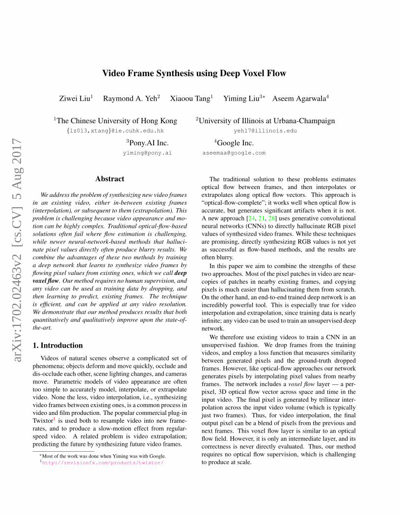
Video Frame Synthesis using Deep Voxel Flow
Ziwei Liu1 Raymond A. Yeh2 Xiaoou Tang1 Yiming Liu3∗ Aseem Agarwala4
1The Chinese University of Hong Kong{lz013,xtang}@ie.cuhk.edu.hk
2University of Illinois at [email protected]
3Pony.AI [email protected]
4Google [email protected]
Abstract
We address the problem of synthesizing new video framesin an existing video, either in-between existing frames(interpolation), or subsequent to them (extrapolation). Thisproblem is challenging because video appearance and mo-tion can be highly complex. Traditional optical-flow-basedsolutions often fail where flow estimation is challenging,while newer neural-network-based methods that halluci-nate pixel values directly often produce blurry results. Wecombine the advantages of these two methods by traininga deep network that learns to synthesize video frames byflowing pixel values from existing ones, which we call deepvoxel flow. Our method requires no human supervision, andany video can be used as training data by dropping, andthen learning to predict, existing frames. The techniqueis efficient, and can be applied at any video resolution.We demonstrate that our method produces results that bothquantitatively and qualitatively improve upon the state-of-the-art.
1. IntroductionVideos of natural scenes observe a complicated set of
phenomena; objects deform and move quickly, occlude anddis-occlude each other, scene lighting changes, and camerasmove. Parametric models of video appearance are oftentoo simple to accurately model, interpolate, or extrapolatevideo. None the less, video interpolation, i.e., synthesizingvideo frames between existing ones, is a common process invideo and film production. The popular commercial plug-inTwixtor1 is used both to resample video into new frame-rates, and to produce a slow-motion effect from regular-speed video. A related problem is video extrapolation;predicting the future by synthesizing future video frames.
∗Most of the work was done when Yiming was with Google.1http://revisionfx.com/products/twixtor/
The traditional solution to these problems estimatesoptical flow between frames, and then interpolates orextrapolates along optical flow vectors. This approach is“optical-flow-complete”; it works well when optical flow isaccurate, but generates significant artifacts when it is not.A new approach [24, 21, 28] uses generative convolutionalneural networks (CNNs) to directly hallucinate RGB pixelvalues of synthesized video frames. While these techniquesare promising, directly synthesizing RGB values is not yetas successful as flow-based methods, and the results areoften blurry.
In this paper we aim to combine the strengths of thesetwo approaches. Most of the pixel patches in video are near-copies of patches in nearby existing frames, and copyingpixels is much easier than hallucinating them from scratch.On the other hand, an end-to-end trained deep network is anincredibly powerful tool. This is especially true for videointerpolation and extrapolation, since training data is nearlyinfinite; any video can be used to train an unsupervised deepnetwork.
We therefore use existing videos to train a CNN in anunsupervised fashion. We drop frames from the trainingvideos, and employ a loss function that measures similaritybetween generated pixels and the ground-truth droppedframes. However, like optical-flow approaches our networkgenerates pixels by interpolating pixel values from nearbyframes. The network includes a voxel flow layer — a per-pixel, 3D optical flow vector across space and time in theinput video. The final pixel is generated by trilinear inter-polation across the input video volume (which is typicallyjust two frames). Thus, for video interpolation, the finaloutput pixel can be a blend of pixels from the previous andnext frames. This voxel flow layer is similar to an opticalflow field. However, it is only an intermediate layer, and itscorrectness is never directly evaluated. Thus, our methodrequires no optical flow supervision, which is challengingto produce at scale.
arX
iv:1
702.
0246
3v2
[cs
.CV
] 5
Aug
201
7
We train our method on the public UCF-101 dataset, buttest it on a wide variety of videos. Our method can beapplied at any resolution, since it is fully convolutional,and produces remarkably high-quality results which aresignificantly better than both optical flow and CNN-basedmethods. While our results are quantitatively better thanexisting methods, this improvement is especially noticeablequalitatively when viewing output videos, since existingquantitative measures are poor at measuring perceptualquality.
2. Related WorkVideo interpolation is commonly used for video re-
timing, novel-view rendering, and motion-based videocompression [29, 18]. Optical flow is the most commonapproach to video interpolation, and frame prediction isoften used to evaluate optical flow accuracy [1]. As such,the quality of flow-based interpolation depends entirely onthe accuracy of flow, which is often challenged by largeand fast motions. Mahajan et al. [20] explore a variationon optical flow that computes paths in the source imagesand copies pixel gradients along them to the interpolatedimages, followed by a Poisson reconstruction. Meyer etal. [22] employ a Eulerian, phase-based approach to inter-polation, but the method is limited to smaller motions.
Convolutional neural networks have been used to makerecent and dramatic improvements in image and videorecognition [17]. They can also be used to predict opticalflow [4], which suggests that CNNs can understand tempo-ral motion. However, these techniques require supervision,i.e., optical flow ground-truth. A related unsupervisedapproach [19] uses a CNN to predict optical flow bysynthesizing interpolated frames, and then inverting theCNN. However, they do not use an optical flow layer inthe network, and their end-goal is to generate optical flow.They do not numerically evaluate the interpolated frames,themselves, and qualitatively the frames appear blurry.
There are a number of papers that use CNNs to directlygenerate images [10] and videos [31, 36]. Blur is oftena problem for these generative techniques, since naturalimages follow a multimodal distribution, while the lossfunctions used often assume a Gaussian distribution. Ourapproach can avoid this blurring problem by copying co-herent regions of pixels from existing frames. GenerativeCNNs can also be used to generate new views of a scenefrom existing photos taken at nearby viewpoints [7, 35].These methods reconstruct images by separately computingdepth and color layers at each hypothesized depth. Thisapproach cannot account for scene motion, however.
Our technical approach is inspired by recent techniquesfor including differentiable motion layers in CNNs [13].Optical flow layers have also been used to render novelviews of objects [38, 14] and change eye gaze direction
while videoconferencing [8]. We apply this approach tovideo interpolation and extrapolation. LSTMs have beenused to extrapolate video [28], but the results can be blurry.Mathieu et al. [21] reduce blurriness by using adversarialtraining [10] and unique loss functions, but the resultsstill contain artifacts (we compare our results against thismethod). Finally, Finn et al. [6] use LSTMs and differ-entiable motion models to better sample the multimodaldistribution of video future predictions. However, theirresults are still blurry, and are trained to videos in veryconstrained scenarios (e.g., a robot arm, or human motionwithin a room from a fixed camera). Our method is ableto produce sharp results for widely diverse videos. Also,we do not pre-align our input videos; other video predictionpapers either assume a fixed camera, or pre-align the input.
3. Our Approach3.1. Deep Voxel Flow
We propose Deep Voxel Flow (DVF) — an end-to-end fully differentiable network for video frame synthesis.The only training data we need are triplets of consecutivevideo frames. During the training process, two frames areprovided as inputs and the remaining frame is used as areconstruction target. Our approach is self-supervised andlearns to reconstruct a frame by borrowing voxels fromnearby frames, which leads to more realistic and sharperresults (Fig. 4) than techniques that hallucinate pixels fromscratch. Furthermore, due to the flexible motion modelingof our approach, no pre-processing (e.g., pre-alignment orlighting adjustment) is needed for the input videos, which isa necessary component for most existing systems [32, 36].
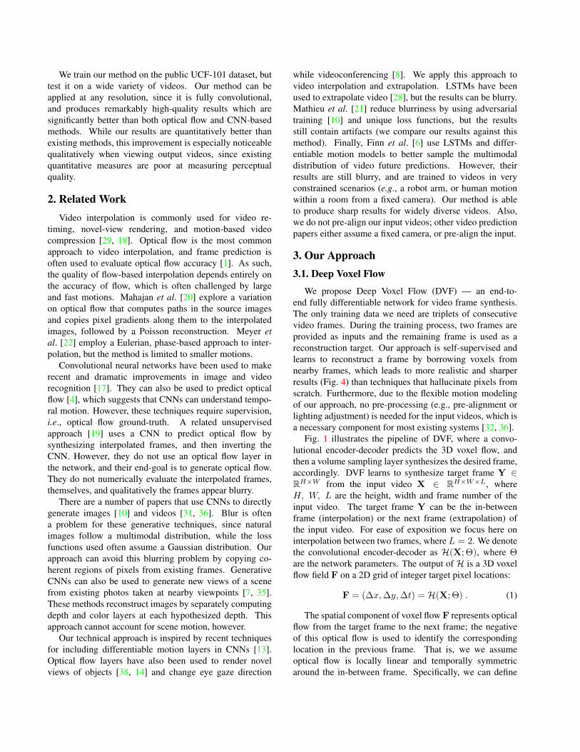
Fig. 1 illustrates the pipeline of DVF, where a convo-lutional encoder-decoder predicts the 3D voxel flow, andthen a volume sampling layer synthesizes the desired frame,accordingly. DVF learns to synthesize target frame Y ∈RH×W from the input video X ∈ RH×W×L, whereH, W, L are the height, width and frame number of theinput video. The target frame Y can be the in-betweenframe (interpolation) or the next frame (extrapolation) ofthe input video. For ease of exposition we focus here oninterpolation between two frames, where L = 2. We denotethe convolutional encoder-decoder as H(X; Θ), where Θare the network parameters. The output of H is a 3D voxelflow field F on a 2D grid of integer target pixel locations:
F = (∆x,∆y,∆t) = H(X; Θ) . (1)
The spatial component of voxel flow F represents opticalflow from the target frame to the next frame; the negativeof this optical flow is used to identify the correspondinglocation in the previous frame. That is, we we assumeoptical flow is locally linear and temporally symmetricaround the in-between frame. Specifically, we can define
Max Pooling Deconvolution Volume SamplingConvolution Skip Connection
Input Video Synthesized FrameConvolutional Encoder-Decoder Voxel Flow
64(relu)
256
256
128
12864
64 32
32
128(relu)
256(relu)
256(relu)
256(relu)
128(relu)
64(relu)
3(tanh)
64
64
128
128
256
256 256
256
𝐗 𝐘�𝐅ℋ(𝐗;Θ)
𝑇𝑥,𝑦,𝑡(𝐗,𝐅)
Figure 1: Pipeline of Deep Voxel Flow (DVF). DVF learns to synthesize a target frame from the input video. The target frame can either bein-between (interpolation) or subsequent to (extrapolation) the input video. DVF adopts a fully-convolutional encoder-decoder architecturecontaining three convolution layers, three deconvolution layers and one bottleneck layer. The only supervision DVF needs is the targetframe which is to be synthesized.
the absolute coordinates of the corresponding locations inthe earlier and later frames as L0 = (x − ∆x, y − ∆y)and L1 = (x + ∆x, y + ∆y), respectively. The temporalcomponent of voxel flow F is a linear blend weight betweenthe previous and next frames to form a color in the targetframe. We use this voxel flow to sample the original inputvideo X with a volume sampling function Tx,y,t to form thefinal synthesized frame Y:
Y = Tx,y,t(X,F) = Tx,y,t(X,H(X; Θ)) . (2)
The volume sampling function samples colors by interpolat-ing within an optical-flow-aligned video volume computedfrom X. Given the corresponding locations (L0,L1), weconstruct a virtual voxel of this volume and use trilinearinterpolation from the colors at the voxel’s corners tocompute an output video color Y(x, y). We compute theinteger locations of the eight vertices of the virtual voxel inthe input video X as:
V000 = (bL0xc, bL0
yc, 0)
V100 = (dL0xe, bL0
yc, 0)
...
V011 = (bL1xc, dL1
ye, 1)
V111 = (dL1xe, dL1
ye, 1) ,
(3)
where b·c is the floor function, and we define the temporalrange for interpolation such that t = 0 for the first inputframe and t = 1 for the second. Given this virtual voxel, the3D voxel flow generates each target voxel Y(x, y) throughtrilinear interpolation:
Y(x, y) = Tx,y,t(X,F) =∑
i,j,k∈[0,1]
WijkX(Vijk) , (4)
Frame 1
Frame 2
Motion Color Key
(a) Ground Truth (b) Voxel Flow (c) Multi-scale Voxel Flow
(d) Difference Image (e) Projected Motion Field (f) Projected Selection Mask
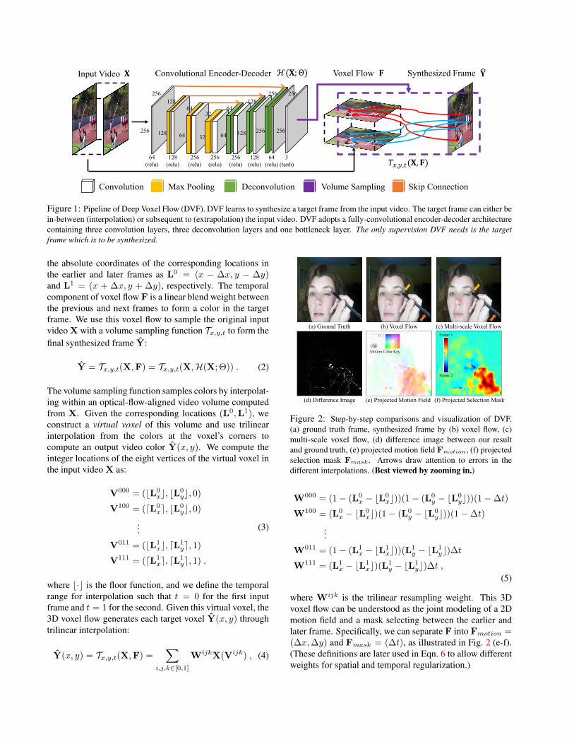
Figure 2: Step-by-step comparisons and visualization of DVF.(a) ground truth frame, synthesized frame by (b) voxel flow, (c)multi-scale voxel flow, (d) difference image between our resultand ground truth, (e) projected motion field Fmotion, (f) projectedselection mask Fmask. Arrows draw attention to errors in thedifferent interpolations. (Best viewed by zooming in.)
W000 = (1− (L0x − bL0
xc))(1− (L0y − bL0
yc))(1−∆t)
W100 = (L0x − bL0
xc)(1− (L0y − bL0
yc))(1−∆t)
...
W011 = (1− (L1x − bL1
xc))(L1y − bL1
yc)∆tW111 = (L1
x − bL1xc)(L1
y − bL1yc)∆t ,
(5)
where Wijk is the trilinear resampling weight. This 3Dvoxel flow can be understood as the joint modeling of a 2Dmotion field and a mask selecting between the earlier andlater frame. Specifically, we can separate F into Fmotion =(∆x,∆y) and Fmask = (∆t), as illustrated in Fig. 2 (e-f).(These definitions are later used in Eqn. 6 to allow differentweights for spatial and temporal regularization.)

Network Architecture. DVF adopts a fully-convolutionalencoder-decoder architecture, containing three convolutionlayers, three deconvolution layers and one bottleneck layer.Therefore, arbitrary-sized videos can be used as inputs forDVF. The network hyperparamters (e.g., the size of featuremaps, the number of channels and activation functions) arespecified in Fig. 1.
For the encoder section of the network, each processingunit contains both convolution and max-pooling. Theconvolution kernel sizes here are 5 × 5, 5 × 5 and 3 ×3, respectively. The bottleneck layer is also connectedby convolution with kernel size 3 × 3. For the decodersection, each processing unit contains bilinear upsamplingand convolution. The convolution kernel sizes here are 3×3,5×5 and 5×5, respectively. To better maintain spatial infor-mation we add skip connections between the correspondingconvolution and deconvolution layers. Specifically, thecorresponding deconvolution layers and convolution layersare concatenated together before being fed forward.
3.2. Learning
For our DVF training, we exploit the l1 reconstructionloss with spatial and temporal coherence regularizations toreduce visual artifacts. Total variation (TV) regularizationsare used here to enforce coherence. Since these regularizersare imposed on the output of the network it can be easilyincorporated into the back-propagation scheme. Our overallobjective function that we minimize is:
L =1
N
∑〈X,Y〉∈D
(‖Y − Tx,y,t(X,F)‖1
+ λ1‖∇Fmotion‖1+ λ2‖∇Fmask‖1
),
(6)
where D is the training set of all frame triplets, N is itscardinality and Y is the target frame to be reconstructed.‖∇Fmotion‖1 is the total variation term on the (x, y)components of voxel flow, and λ1 is the corresponding reg-ularization weight; similarly, ‖∇Fmask‖1 is the regularizeron the temporal component of voxel flow, and λ2 its weight.(We experimentally found it useful to weight the coherenceof the spatial component of the flow more strongly thanthe temporal selection.) To optimize the l1 norm, we usethe Charbonnier penalty function Φ(x) = (x2 + ε2)1/2
for approximation. Here we empirically set λ1 = 0.01,λ2 = 0.005 and ε = 0.001.
We initialize the weights in DVF using Gaussian dis-tribution with standard deviation of 0.01. Learning thenetwork is achieved via ADAM solver [16] with learningrate of 0.0001, β1 = 0.9, β2 = 0.999 and batch size of 32.Batch normalization [12] is adopted for faster convergence.Differentiable Volume Sampling. To make our DVFan end-to-end fully differentiable system, we define the
Input Video (scale 0)
Convolutional Encoder-Decoder(scale 0)
𝐅0
Max Pooling DeconvolutionConvolution Skip Connection
Concatenation
𝐅𝟏𝒙,𝒚
Upsampling
963232 32 64 3
256256 256
256
22
256
256
128128
2 6464
2 𝐅𝟐𝒙,𝒚
Figure 3: Pipeline of multi-scale Deep Voxel Flow. A seriesof convolutional encoder-decoder networks work on video framesfrom a coarse to fine scale. The spatial components of the 3Dvoxel flow computed at lower resolutions (here, 128 × 128 and64 × 64) are upsampled to 256 × 256 and then convolved to 32channels. The three different resolutions are then concatenated toform a 256 × 256 × 96 layer, and finally passed through severalconvolutional layers to form a final 256×256×3 voxel flow field.
gradients with respect to 3D voxel flow F = (∆x,∆y,∆t)so that the reconstruction error can be backpropagatedthrough a volume sampling layer. Similar to [13], the partialderivative of the synthesized voxel color Y(x, y) w.r.t. ∆xis
∂Y(x, y)
∂(∆x)=
∑i,j,k∈[0,1]
EijkX(Vijk) , (7)
E000 = (1− (L0y − bL0
yc))(1−∆t)
E100 = − (1− (L0y − bL0
yc))(1−∆t)
...
E011 = − (L1y − bL1
yc)∆tE111 = (L1
y − bL1yc)∆t ,
(8)
where Eijk is the error reassignment weight w.r.t.∆x. Similarly, we can compute ∂Y(x, y)/∂(∆y) and∂Y(x, y)/∂(∆t). This gives us a sub-differentiable sam-pling mechanism, allowing loss gradients to flow back tothe 3D voxel flow F. This sampling mechanism can beimplemented very efficiently by just looking at the kernelsupport region for each output voxel.
3.3. Multi-scale Flow Fusion
As stated in Sec. 3.2, the gradients of reconstructionerror are obtained by only looking at the kernel supportregion for each output voxel, which makes it hard to findlarge motions that fall outside the kernel. Therefore, wepropose a multi-scale Deep Voxel Flow (multi-scale DVF)to better encode both large and small motions.
Specifically, we have a series of convolutional encoder-decoder HN ,HN−1, · · · ,H0 working on video framesfrom coarse scale sN to fine scale s0, respectively. Typ-ically, in our experiments, we set s2 = 64 × 64, s1 =
Frame 1 Frame 2Interpolated Frames (Ours)
(b)Ground Truth OursBeyond MSE
Frame 1 Frame 2Interpolated Frame
(a)
(d)
Frame 1 Frame 2 Extrapolated Frames (Ours)Frame 1 Frame 2 Extrapolated Frame
Ground Truth OursBeyond MSE(c)
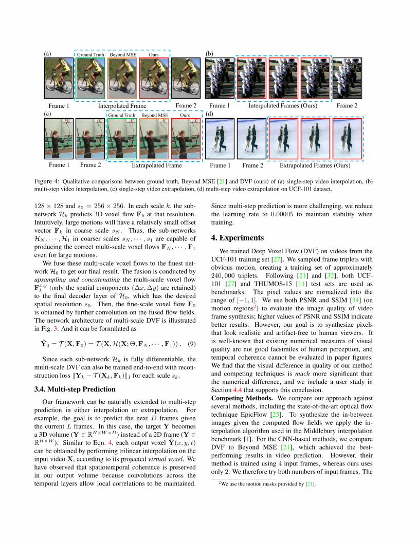
Figure 4: Qualitative comparisons between ground truth, Beyond MSE [21] and DVF (ours) of (a) single-step video interpolation, (b)multi-step video interpolation, (c) single-step video extrapolation, (d) multi-step video extrapolation on UCF-101 dataset.
128 × 128 and s0 = 256 × 256. In each scale k, the sub-network Hk predicts 3D voxel flow Fk at that resolution.Intuitively, large motions will have a relatively small offsetvector Fk in coarse scale sN . Thus, the sub-networksHN , · · · ,H1 in coarser scales sN , · · · , s1 are capable ofproducing the correct multi-scale voxel flows FN , · · · ,F1
even for large motions.We fuse these multi-scale voxel flows to the finest net-
work H0 to get our final result. The fusion is conducted byupsampling and concatenating the multi-scale voxel flowFx,y
k (only the spatial components (∆x,∆y) are retained)to the final decoder layer of H0, which has the desiredspatial resolution s0. Then, the fine-scale voxel flow F0
is obtained by further convolution on the fused flow fields.The network architecture of multi-scale DVF is illustratedin Fig. 3. And it can be formulated as
Y0 = T (X,F0) = T (X,H(X; Θ,FN , · · · ,F1)) . (9)
Since each sub-network Hk is fully differentiable, themulti-scale DVF can also be trained end-to-end with recon-struction loss ‖Yk − T (Xk,Fk)‖1 for each scale sk.
3.4. Multi-step Prediction
Our framework can be naturally extended to multi-stepprediction in either interpolation or extrapolation. Forexample, the goal is to predict the next D frames giventhe current L frames. In this case, the target Y becomesa 3D volume (Y ∈ RH×W×D) instead of a 2D frame (Y ∈RH×W ). Similar to Eqn. 4, each output voxel Y(x, y, t)can be obtained by performing trilinear interpolation on theinput video X, according to its projected virtual voxel. Wehave observed that spatiotemporal coherence is preservedin our output volume because convolutions across thetemporal layers allow local correlations to be maintained.
Since multi-step prediction is more challenging, we reducethe learning rate to 0.00005 to maintain stability whentraining.
4. ExperimentsWe trained Deep Voxel Flow (DVF) on videos from the
UCF-101 training set [27]. We sampled frame triplets withobvious motion, creating a training set of approximately240, 000 triplets. Following [21] and [32], both UCF-101 [27] and THUMOS-15 [11] test sets are used asbenchmarks. The pixel values are normalized into therange of [−1, 1]. We use both PSNR and SSIM [34] (onmotion regions2) to evaluate the image quality of videoframe synthesis; higher values of PSNR and SSIM indicatebetter results. However, our goal is to synthesize pixelsthat look realistic and artifact-free to human viewers. Itis well-known that existing numerical measures of visualquality are not good facsimiles of human perception, andtemporal coherence cannot be evaluated in paper figures.We find that the visual difference in quality of our methodand competing techniques is much more significant thanthe numerical difference, and we include a user study inSection 4.4 that supports this conclusion.Competing Methods. We compare our approach againstseveral methods, including the state-of-the-art optical flowtechnique EpicFlow [25]. To synthesize the in-betweenimages given the computed flow fields we apply the in-terpolation algorithm used in the Middlebury interpolationbenchmark [1]. For the CNN-based methods, we compareDVF to Beyond MSE [21], which achieved the best-performing results in video prediction. However, theirmethod is trained using 4 input frames, whereas ours usesonly 2. We therefore try both numbers of input frames. The
2We use the motion masks provided by [21].
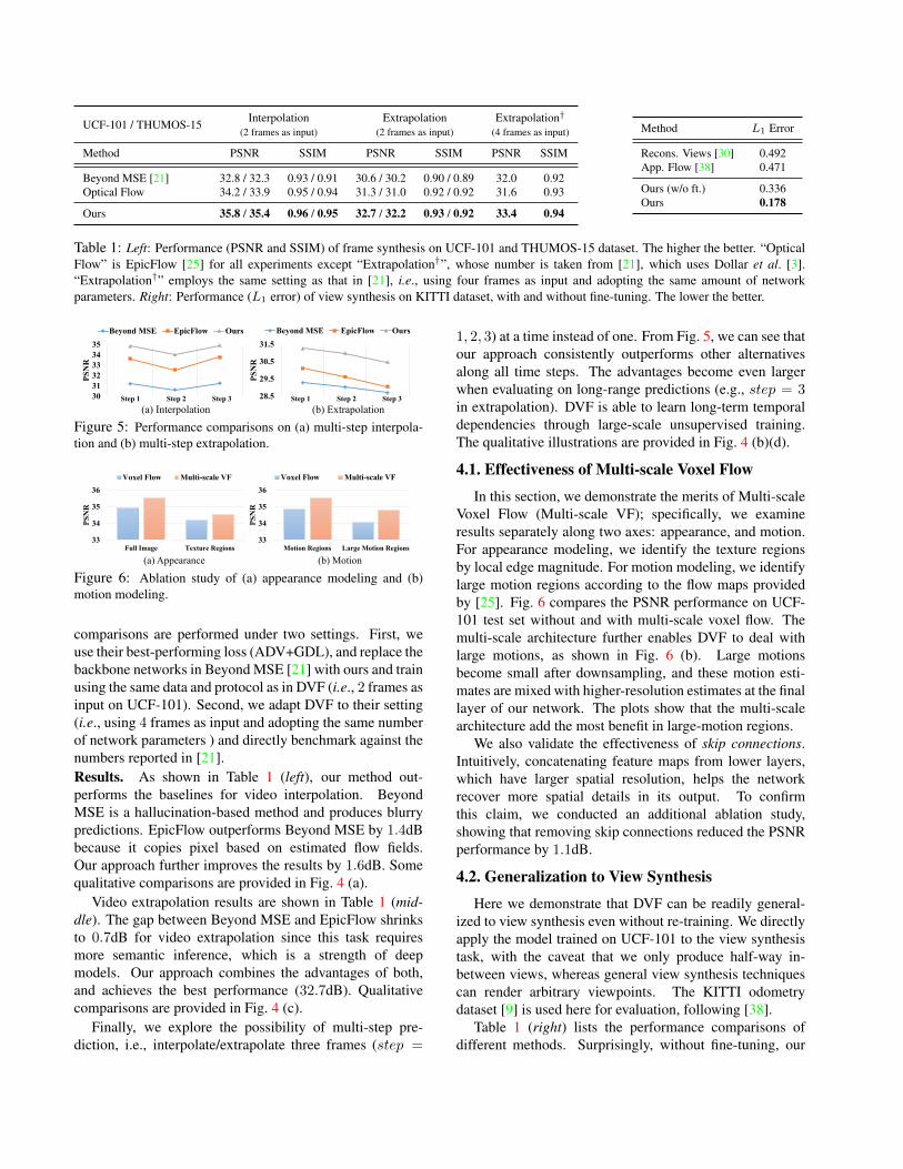
UCF-101 / THUMOS-15 Interpolation Extrapolation Extrapolation†
(2 frames as input) (2 frames as input) (4 frames as input)
Method PSNR SSIM PSNR SSIM PSNR SSIM
Beyond MSE [21] 32.8 / 32.3 0.93 / 0.91 30.6 / 30.2 0.90 / 0.89 32.0 0.92Optical Flow 34.2 / 33.9 0.95 / 0.94 31.3 / 31.0 0.92 / 0.92 31.6 0.93
Ours 35.8 / 35.4 0.96 / 0.95 32.7 / 32.2 0.93 / 0.92 33.4 0.94
Method L1 Error
Recons. Views [30] 0.492App. Flow [38] 0.471
Ours (w/o ft.) 0.336Ours 0.178
Table 1: Left: Performance (PSNR and SSIM) of frame synthesis on UCF-101 and THUMOS-15 dataset. The higher the better. “OpticalFlow” is EpicFlow [25] for all experiments except “Extrapolation†”, whose number is taken from [21], which uses Dollar et al. [3].“Extrapolation†” employs the same setting as that in [21], i.e., using four frames as input and adopting the same amount of networkparameters. Right: Performance (L1 error) of view synthesis on KITTI dataset, with and without fine-tuning. The lower the better.
303132333435
PSN
R
Beyond MSE EpicFlow Ours
28.5
29.5
30.5
31.5
PSN
R
Beyond MSE EpicFlow Ours
(a) Interpolation (b) ExtrapolationStep 1 Step 2 Step 3 Step 1 Step 2 Step 3
Figure 5: Performance comparisons on (a) multi-step interpola-tion and (b) multi-step extrapolation.
33
34
35
36
Full Image Texture Regions
PSN
R
Voxel Flow Multi-scale VF
33
34
35
36
Motion Regions Large Motion Regions
PSN
R
Voxel Flow Multi-scale VF
(a) Appearance (b) Motion
Figure 6: Ablation study of (a) appearance modeling and (b)motion modeling.
comparisons are performed under two settings. First, weuse their best-performing loss (ADV+GDL), and replace thebackbone networks in Beyond MSE [21] with ours and trainusing the same data and protocol as in DVF (i.e., 2 frames asinput on UCF-101). Second, we adapt DVF to their setting(i.e., using 4 frames as input and adopting the same numberof network parameters ) and directly benchmark against thenumbers reported in [21].Results. As shown in Table 1 (left), our method out-performs the baselines for video interpolation. BeyondMSE is a hallucination-based method and produces blurrypredictions. EpicFlow outperforms Beyond MSE by 1.4dBbecause it copies pixel based on estimated flow fields.Our approach further improves the results by 1.6dB. Somequalitative comparisons are provided in Fig. 4 (a).
Video extrapolation results are shown in Table 1 (mid-dle). The gap between Beyond MSE and EpicFlow shrinksto 0.7dB for video extrapolation since this task requiresmore semantic inference, which is a strength of deepmodels. Our approach combines the advantages of both,and achieves the best performance (32.7dB). Qualitativecomparisons are provided in Fig. 4 (c).
Finally, we explore the possibility of multi-step pre-diction, i.e., interpolate/extrapolate three frames (step =
1, 2, 3) at a time instead of one. From Fig. 5, we can see thatour approach consistently outperforms other alternativesalong all time steps. The advantages become even largerwhen evaluating on long-range predictions (e.g., step = 3in extrapolation). DVF is able to learn long-term temporaldependencies through large-scale unsupervised training.The qualitative illustrations are provided in Fig. 4 (b)(d).
4.1. Effectiveness of Multi-scale Voxel Flow
In this section, we demonstrate the merits of Multi-scaleVoxel Flow (Multi-scale VF); specifically, we examineresults separately along two axes: appearance, and motion.For appearance modeling, we identify the texture regionsby local edge magnitude. For motion modeling, we identifylarge motion regions according to the flow maps providedby [25]. Fig. 6 compares the PSNR performance on UCF-101 test set without and with multi-scale voxel flow. Themulti-scale architecture further enables DVF to deal withlarge motions, as shown in Fig. 6 (b). Large motionsbecome small after downsampling, and these motion esti-mates are mixed with higher-resolution estimates at the finallayer of our network. The plots show that the multi-scalearchitecture add the most benefit in large-motion regions.
We also validate the effectiveness of skip connections.Intuitively, concatenating feature maps from lower layers,which have larger spatial resolution, helps the networkrecover more spatial details in its output. To confirmthis claim, we conducted an additional ablation study,showing that removing skip connections reduced the PSNRperformance by 1.1dB.
4.2. Generalization to View Synthesis
Here we demonstrate that DVF can be readily general-ized to view synthesis even without re-training. We directlyapply the model trained on UCF-101 to the view synthesistask, with the caveat that we only produce half-way in-between views, whereas general view synthesis techniquescan render arbitrary viewpoints. The KITTI odometrydataset [9] is used here for evaluation, following [38].
Table 1 (right) lists the performance comparisons ofdifferent methods. Surprisingly, without fine-tuning, our

Appearance FlowGround Truth Ours
(c)
(d)
(a)
(b)
Interpolated View (Ours)View 1 View 2
Figure 7: Several examples and comparisons for view synthesison the KITTI dataset. Rows (a-b) show two examples of interpo-lating large viewpoint changes. Rows (c-d) compare ground truth,Appearance Flow, and our method for two other examples. Ourmethod performs better than Appearance Flow, e.g., on the streetlamp (c) and trees (d).
Method EPE
LD Flow [2] 12.4B. Basics [37] 9.9FlowNet [5] 9.1EpicFlow [25] 3.8
Ours (w/o ft.) 14.6Ours 9.5
Method Acc.
Random 39.1Unsup. Video [33] 43.8Shuffle&Learn [23] 50.2ImageNet [15] 63.3
Ours (w/o ft.) 48.7Ours 52.4
Table 2: Left: Endpoint error of flow estimation on KITTI dataset.The lower the better. Right: Classification accuracy of actionrecognition on UCF-101 dataset, with and without fine-tuning.The higher the better. Note that our method is fully unsupervised.
approach already outperforms [30] and [38] by 0.164 and0.135 respectively. We find that fine-tuning on the KIITItraining set could further reduce the reconstruction error.Note that KITTI dataset exhibits large camera motion,which is much different from our original training data.(UCF-101 mainly focuses on human actions.) This observa-tion implies that voxel flow has good generalization abilityand can be used as a universal frame/view synthesizer. Thequalitative comparisons are provided in Fig. 7.
4.3. Frame Synthesis as Self-Supervision
In addition to making progress on the quality of video in-terpolation/extrapolation, we demonstrate that video framesynthesis can serve as a self-supervision task for represen-tation learning. Here, the internal representation learned byDVF is applied to unsupervised flow estimation and pre-training of action recognition.As Unsupervised Flow Estimation. Recall that 3D voxel
flow can be projected into a 2D motion field, which isillustrated in Fig. 2 (e). We quantitatively evaluate the flowestimation of DVF by comparing the projected 2D motionfield to the ground truth optical flow field. The KITTI flow2012 dataset [9] is used as a test set. Table 2 (left) reportsthe average endpoint error (EPE) over all the labeled pixels.After fine-tuning, the unsupervised flow generated by DVFsurpasses traditional methods [2] and performs comparablyto some of the supervised deep models [5]. Learning tosynthesize frames on a large-scale video corpus can encodeessential motion information into our model.As Unsupervised Representation Learning. Here wereplace the reconstruction layers in DVF with classificationlayers (i.e., fully-connected layer + softmax loss). Themodel is fine-tuned and tested with an action recognitionloss on the UCF-101 dataset (split-1) [27]. This is equiva-lent to using frame synthesis by voxel flow as a pre-trainingtask. As demonstrated in Table 2 (right), our approachoutperforms random initialization by a large margin andalso shows superior performance to other representationlearning alternatives [33]. To synthesize frames using voxelflow, DVF has to encode both appearance and motion infor-mation, which implicitly mimics a two-stream CNN [26].
4.4. Applications
DVF can be used to produce slow-motion effects onhigh-definition (HD) videos. We collect HD videos (1080×720, 30fps) from the web with various content and motiontypes as our real-world benchmark. We drop every otherframe to act as ground truth. Note that the model usedhere is trained on the UCF-101 dataset without any furtheradaptation. Since the DVF is fully-convolutional, it can beapplied to videos of an arbitrary size. More video qualitycomparisons are available on our project page3.Visual Comparisons. Existing video slo-mo softwarerelies on explicit optical flow estimation to generate in-between frames. Thus, we choose EpicFlow [25] to serveas a strong baseline. Fig. 8 illustrates slo-mo effects on the“Throw” and “Street” sequences, respectively. Both tech-niques tend to produce spatially coherent results, though ourmethod performs even better. For example, in the “Throw”sequence, DVF maintains the structure of the logo, while inthe “Street” sequence, DVF can better handle the occlusionbetween the pedestrian and the advertisement. However,the advantage is much more obvious when the temporalaxis is examined. We show this advantage in static formby showing xt slices of the interpolated videos (Fig. 8(c)); the EpicFlow results are much more jagged acrosstime. Our observation is that EpicFlow often produces zero-length flow vectors for confusing motions, leading to spatialcoherence but temporal discontinuities. Deep learning is,
3https://liuziwei7.github.io/projects/VoxelFlow

(a)
(b)
EpicFlow OursGround Truth
𝑥
𝑡
𝑥
𝑡
𝑥
𝑡
𝑥
𝑡
𝑥
𝑡
𝑥
𝑡EpicFlow OursGround Truth
Figure 8: Visual quality comparisons between EpicFlow, ground truth and our approach. Row (a) shows several single frames from theoutput videos. Row (b) shows close-ups of xt slices of each output video (rather than single frames, which are xy slices). From thisvisualization, it can be seen that the EpicFlow output is more jagged across time.
Booth Dog Kids Park Throw Street Sky Baseball Subway Balloon
EpicFlow Ground Truth Ours
(a) (b)Diagonal-split Comparison
Method 1 \ Method 20%
10%20%30%40%50%60%70%80%90%
100%
Pref
eren
ce P
erce
ntag
e
Figure 9: (a) Side-by-side comparison of video sequences with a diagonal-split stitch (order randomized), (b) user study results of ourapproach against both EpicFlow and ground truth. 95% confidence intervals are used as error bars.
in general, able to produce more temporally smooth resultsthan linearly scaling optical flow vectors.
User Study. We conducted a user study on the final slo-mo video sequences to objectively compare the qualityof different methods. We compare DVF against bothEpicFlow and ground truth. For side-by-side comparisons,synthesized videos of the two different methods are stitchedtogether using a diagonal split, as illustrated in Fig. 9 (a).The left/right positions are randomly placed. Twenty sub-jects were enrolled in this user study; they had no previousexperience with computer vision. We asked participants toselect their preferences on 10 stitched video sequences, i.e.,to determine whether the left-side or right-side videos weremore visually pleasant. As Fig. 9 (b) shows, our approachis significantly preferred to EpicFlow among all testingsequences. For the null hypothesis: “there is no differencebetween EpicFlow results and our results”, the p-value isp < 0.00001, and the hypothesis can be safely rejected.Moreover, for half of the sequences participants choose theresult of our method roughly equally as often as the groundtruth, which suggests that they are of equal visual quality.For the null hypothesis: “there is no difference betweenour results and ground truth”, the p-value is 0.838193;statistical significance is not reached to safely reject the nullhypothesis in this case. Overall, we conclude that DVF iscapable of generating high-quality slo-mo effects across a
wide range of videos.Failure Cases. The most typical failure mode of DVF is inscenes with repetitive patterns (e.g., the “Park” sequence).In these cases, it is ambiguous to determine the true sourcevoxel to copy by just referring to RGB differences. Strongerregularization terms can be added to address this problem.
5. Discussion
In this paper, we propose an end-to-end deep network,Deep Voxel Flow (DVF), for video frame synthesis. Ourmethod is able to copy pixels from existing video frames,rather than hallucinate them from scratch. On the otherhand, our method can be trained in an unsupervised mannerusing any video. Our experiments show that this approachimproves upon both optical flow and recent CNN tech-niques for interpolating and extrapolating video. In thefuture, it may useful to combine flow layers with puresynthesis layers to better predict pixels that cannot becopied from other video frames. Also, the way we extendour method to multi-frame prediction is fairly simple; thereare a number of interesting alternatives, such as usingthe desired temporal step (e.g., t = .25 for the first outof three interpolated frames) as an input to the network.Compressing our network so that it may be run on a mobiledevice is also a direction we hope to explore.
References[1] S. Baker, D. Scharstein, J. Lewis, S. Roth, M. J. Black, and
R. Szeliski. A database and evaluation methodology foroptical flow. IJCV, 92(1), 2011. 2, 5
[2] T. Brox and J. Malik. Large displacement optical flow:descriptor matching in variational motion estimation. T-PAMI, 33(3), 2011. 7
[3] P. Dollar. Piotr’s Computer Vision Matlab Toolbox (PMT).https://github.com/pdollar/toolbox. 6
[4] A. Dosovitskiy, P. Fischer, E. Ilg, P. Hausser, C. Hazirbas,V. Golkov, P. v.d. Smagt, D. Cremers, and T. Brox. Flownet:Learning optical flow with convolutional networks. In ICCV,2015. 2
[5] A. Dosovitskiy, P. Fischery, E. Ilg, C. Hazirbas, V. Golkov,P. van der Smagt, D. Cremers, T. Brox, et al. Flownet:Learning optical flow with convolutional networks. In ICCV,2015. 7
[6] C. Finn, I. Goodfellow, and S. Levine. Unsupervisedlearning for physical interaction through video prediction. InNIPS, 2016. 2
[7] J. Flynn, I. Neulander, J. Philbin, and N. Snavely. Deep-stereo: Learning to predict new views from the world’simagery. In CVPR, 2016. 2
[8] Y. Ganin, D. Kononenko, D. Sungatullina, and V. Lempitsky.Deepwarp: Photorealistic image resynthesis for gaze manip-ulation. In ECCV, 2016. 2
[9] A. Geiger, P. Lenz, and R. Urtasun. Are we ready forautonomous driving? the kitti vision benchmark suite. InCVPR, 2012. 6, 7
[10] I. Goodfellow, J. Pouget-Abadie, M. Mirza, B. Xu,D. Warde-Farley, S. Ozair, A. Courville, and Y. Bengio.Generative adversarial nets. In NIPS. 2014. 2
[11] A. Gorban, H. Idrees, Y.-G. Jiang, A. Roshan Zamir,I. Laptev, M. Shah, and R. Sukthankar. THUMOS challenge:Action recognition with a large number of classes, 2015. 5
[12] S. Ioffe and C. Szegedy. Batch normalization: Acceleratingdeep network training by reducing internal covariate shift. InICML, 2015. 4
[13] M. Jaderberg, K. Simonyan, A. Zisserman, et al. Spatialtransformer networks. In NIPS, 2015. 2, 4
[14] D. Ji, J. Kwon, M. McFarland, and S. Savarese. Deep viewmorphing. In CVPR, 2017. 2
[15] A. Karpathy, G. Toderici, S. Shetty, T. Leung, R. Sukthankar,and L. Fei-Fei. Large-scale video classification with convo-lutional neural networks. In CVPR, 2014. 7
[16] D. Kingma and J. Ba. Adam: A method for stochasticoptimization. In ICLR, 2015. 4
[17] A. Krizhevsky, I. Sutskever, and G. E. Hinton. Imagenetclassification with deep convolutional neural networks. InNIPS, 2012. 2
[18] Z. Liu, L. Yuan, X. Tang, M. Uyttendaele, and J. Sun. Fastburst images denoising. TOG, 33(6), 2014. 2
[19] G. Long, L. Kneip, J. M. Alvarez, H. Li, X. Zhang, andQ. Yu. Learning image matching by simply watching video.In ECCV, 2016. 2
[20] D. Mahajan, F.-C. Huang, W. Matusik, R. Ramamoorthi, andP. Belhumeur. Moving gradients: A path-based method forplausible image interpolation. TOG, 28(3), 2009. 2
[21] M. Mathieu, C. Couprie, and Y. LeCun. Deep multi-scalevideo prediction beyond mean square error. In ICLR, 2016.1, 2, 5, 6
[22] S. Meyer, O. Wang, H. Zimmer, M. Grosse, and A. Sorkine-Hornung. Phase-based frame interpolation for video. InCVPR, 2015. 2
[23] I. Misra, C. L. Zitnick, and M. Hebert. Shuffle and learn:unsupervised learning using temporal order verification. InECCV, 2016. 7
[24] M. Ranzato, A. Szlam, J. Bruna, M. Mathieu, R. Collobert,and S. Chopra. Video (language) modeling: a baselinefor generative models of natural videos. arXiv preprintarXiv:1412.6604, 2014. 1
[25] J. Revaud, P. Weinzaepfel, Z. Harchaoui, and C. Schmid.Epicflow: Edge-preserving interpolation of correspondencesfor optical flow. In CVPR, 2015. 5, 6, 7
[26] K. Simonyan and A. Zisserman. Two-stream convolutionalnetworks for action recognition in videos. In NIPS, 2014. 7
[27] K. Soomro, A. Roshan Zamir, and M. Shah. UCF101: Adataset of 101 human actions classes from videos in the wild.In CRCV-TR-12-01, 2012. 5, 7
[28] N. Srivastava, E. Mansimov, and R. Salakhutdinov. Unsu-pervised learning of video representations using lstms. InICML, 2015. 1, 2
[29] R. Szeliski. Prediction error as a quality metric for motionand stereo. In ICCV, 1999. 2
[30] M. Tatarchenko, A. Dosovitskiy, and T. Brox. Multi-view 3dmodels from single images with a convolutional network. InECCV, 2016. 6, 7
[31] C. Vondrick, H. Pirsiavash, and A. Torralba. GeneratingVideos with Scene Dynamics. In NIPS. 2016. 2
[32] J. Walker, C. Doersch, A. Gupta, and M. Hebert. An uncer-tain future: Forecasting from static images using variationalautoencoders. In ECCV, 2016. 2, 5
[33] X. Wang and A. Gupta. Unsupervised learning of visualrepresentations using videos. In ICCV, 2015. 7
[34] Z. Wang, A. C. Bovik, H. R. Sheikh, and E. P. Simoncelli.Image quality assessment: from error visibility to structuralsimilarity. TIP, 13(4), 2004. 5
[35] J. Xie, R. B. Girshick, and A. Farhadi. Deep3d: Fully au-tomatic 2d-to-3d video conversion with deep convolutionalneural networks. In ECCV, 2016. 2
[36] T. Xue, J. Wu, K. L. Bouman, and W. T. Freeman. Visualdynamics: Probabilistic future frame synthesis via crossconvolutional networks. In NIPS, 2016. 2
[37] J. J. Yu, A. W. Harley, and K. G. Derpanis. Back tobasics: Unsupervised learning of optical flow via brightnessconstancy and motion smoothness. In ECCV Workshop onBrave New Ideas in Motion Representations, 2016. 7
[38] T. Zhou, S. Tulsiani, W. Sun, J. Malik, and A. A. Efros. Viewsynthesis by appearance flow. In ECCV, 2016. 2, 6, 7