vibrations using matlab
TRANSCRIPT

8/20/2019 Vibrations Using Matlab
http://slidepdf.com/reader/full/vibrations-using-matlab 1/170
Simple Vibration Problems with MATLAB (and
Some Help from MAPLE)
Original Version by Stephen Kuchnicki
December 7, 2009

8/20/2019 Vibrations Using Matlab
http://slidepdf.com/reader/full/vibrations-using-matlab 2/170
Contents
Preface ix
1 Introduction 1
2 SDOF Undamped Oscillation 3
3 A Damped SDOF System 11
4 Overdamped SDOF Oscillation 17
5 Harmonic Excitation of Undamped SDOF Systems 23
6 Harmonic Forcing of Damped SDOF Systems 33
7 Base Excitation of SDOF Systems 39
8 SDOF Systems with a Rotating Unbalance 51
9 Impulse Response of SDOF Systems 61
10 Step Response of a SDOF System 67
11 Response of SDOF Systems to Square Pulse Inputs 77
12 Response of SDOF System to Ramp Input 89
13 SDOF Response to Arbitrary Periodic Input 95
14 Free Vibration of MDOF Systems 101
15 Damping of MDOF Systems 113
16 A Universal Vibration Solver 123
17 Modeling a van der Pol Oscillator 133
18 Random Vibration and Matlab 141
v

8/20/2019 Vibrations Using Matlab
http://slidepdf.com/reader/full/vibrations-using-matlab 3/170
vi CONTENTS
19 Randomly-Excited Du¢ng Oscillator 149
20 Monte Carlo Simulation of a Random System 157
21 Conclusion 165

8/20/2019 Vibrations Using Matlab
http://slidepdf.com/reader/full/vibrations-using-matlab 4/170
Preface
This document is companion to the text: Mechanical Vibration: Analysis, Un-certainties and Control, by Haym Benaroya and Mark Nagurka, CRC Press2010; contact: [email protected]; [email protected]
ix

8/20/2019 Vibrations Using Matlab
http://slidepdf.com/reader/full/vibrations-using-matlab 5/170

8/20/2019 Vibrations Using Matlab
http://slidepdf.com/reader/full/vibrations-using-matlab 6/170
Chapter 1
Introduction
This document is intended as a companion to Mechanical Vibration: Analy-sis, Uncertainties, and Control by Haym Benaroya and Mark Nagurka. Thiscompanion draws heavily upon the Matlab software package, produced by theMathWorks, Inc. We do not intend to teach Matlab in this work; rather, wewish to show how a vizualization tool like Matlab can be used to aid in solutionof vibration problems, and hopefully to provide both the novice and the experi-enced Matlab programmer a few new tricks with which to attack their problemsof interest.
Matlab (Mat rix Laboratory) was born from the LINPACK routines writtenfor use with C and Fortran. The Matlab package provides both command-lineand programming language interfaces, allowing the user to test simple state-ments at the command prompt, or to run complicated codes by calling a func-tion name. Matlab is excellent for handling matrix quantities because it as-sumes every variable is an array. Thus, calling on the multiplication operatoralone causes Matlab to attempt matrix, not scalar multiplication. Also, Mat-lab includes special “array operators” that allow multiplication of arrays on anelement-by-element basis. For example, if we set the variable a = [1 2 3] andb = [4 5 6]; we can perform the matrix multiplications:
c = a b0 (1.1)
d = a0 b (1.2)
(Note that the apostrophe is the transpose operator in Matlab.) The resultc would be a scalar (speci…cally, 32): The variable d would contain a 3-by-3matrix, whose rows would be scalar multiples of b: However, what if the values
stored in a are three masses, and those in b their corresponding accelerations?If we wished to …nd the force on each mass, we would need to multiply the…rst element of a by the …rst element of b; and so on for the second and thirdelements. Matlab provides “array multiplication” for such an instance:
e = a: b (1.3)
1

8/20/2019 Vibrations Using Matlab
http://slidepdf.com/reader/full/vibrations-using-matlab 7/170
2 CHAPTER 1 INTRODUCTION
Take special note of the period between a and the asterisk. This tells Matlabto ignore its usual matrix multiplication rules, and instead create e by multi-
plying the corresponding elements of a and b: The result here would be e = [410 18]: This is one of the more useful specialized commands in Matlab, and onewe will use frequently. Other commands will be discussed as they arise.
The vast majority of these examples will use Matlab in its programmingmode. The general format is to introduce a problem, with reference to thetext where applicable, and to show the analytic solution (if derivable). Several…gures follow each example, showing results of each vibration problem underdi¤erent sets of parameters and making use of Matlab’s integrated graphicscapabilities. Finally, the Matlab code used to generate the …gures is presented,with comments explaining what was done, why it was done, and other waysit could have been done in Matlab. The code should look somewhat familiarto those who have used C and Fortran in the past; Matlab’s language sharesseveral common structures with both of these languages, making it relativelyeasy for an experienced C or Fortran programmer to learn Matlab.
One distinction to make with Matlab programming is between script m-…lesand function m-…les. Both are sets of commands that are saved in a …le. Thedi¤erences are that variables used in a script …le are retained in the Matlabworkspace and can be called upon after the script completes. Variables within afunction m-…le cannot be used outside of the function unless they are returned(much like C functions or Fortran subroutines). Additionally, a function mustbegin with the line function output = function_name(var1;var2; :::varN ).This line tells the Matlab interpreter that this …le is a function separate fromthe workspace. (Again, the form should look familiar to Fortran and C pro-grammers.)

8/20/2019 Vibrations Using Matlab
http://slidepdf.com/reader/full/vibrations-using-matlab 8/170
Chapter 2
SDOF Undamped
Oscillation
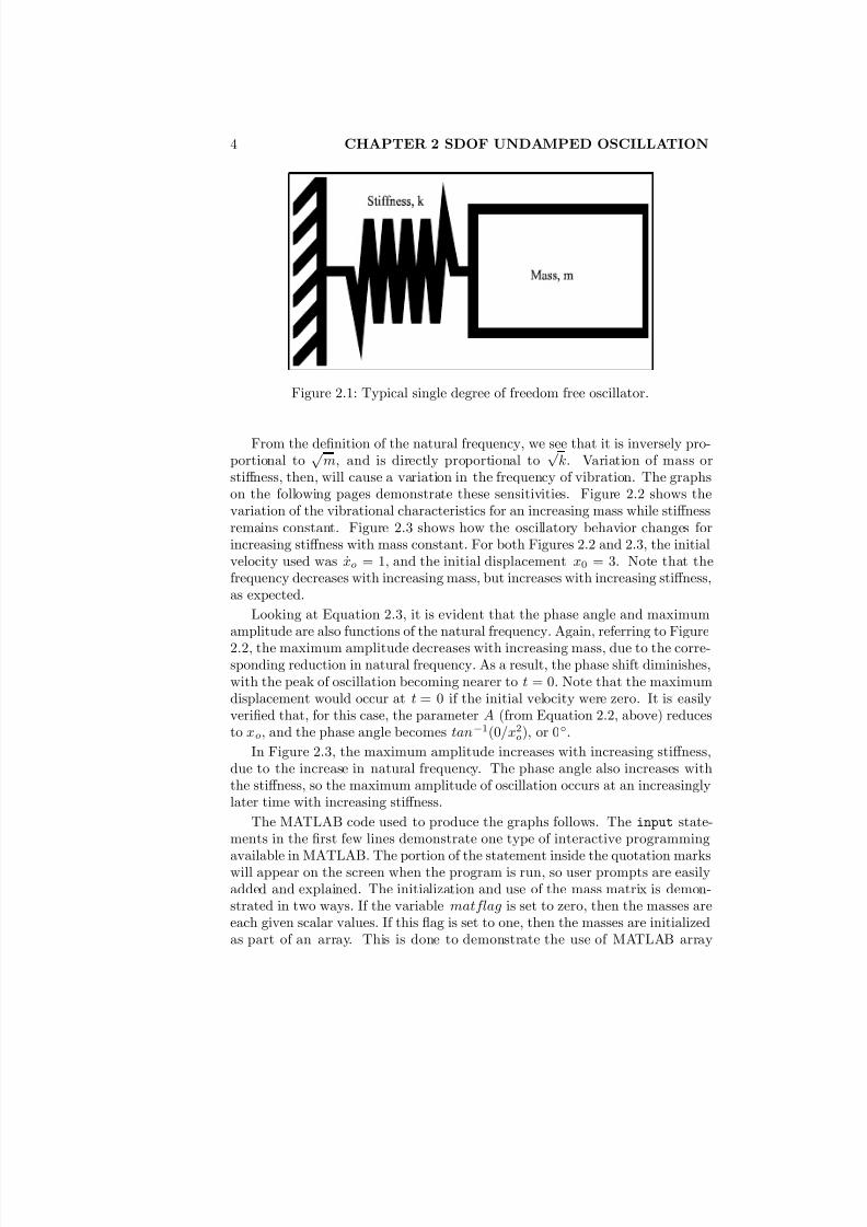
The simplest form of vibration that we can study is the single degree of freedomsystem without damping or external forcing. A sample of such a system is shownin Figure 2.1. A free-body analysis of this system in the framework of Newton’ssecond law, as performed in Chapter 2 of the textbook, results in the followingequation of motion:
m::x + kx = 0: (2.1)
(In general, we would have the forcing function F (t) on the right-hand side;it’s assumed zero for this analysis.) Dividing through by m; and introducingthe parameter !n =
p k=m; we obtain a solution of the form
x(t) = A sin(!nt + ); (2.2)
or, in terms of the physical parameters of the system, we have
x(t) = p !2nx2
o + _x2o
!ncos(!nt tan1 _xo
!nxo): (2.3)
From this, we see that the complete response of an undamped, unforced, onedegree of freedom oscillator depends on three physical parameters: !n, xo, and_xo: the natural frequency, initial velocity, and initial displacement, respectively.
3
8/20/2019 Vibrations Using Matlab
http://slidepdf.com/reader/full/vibrations-using-matlab 9/170
4 CHAPTER 2 SDOF UNDAMPED OSCILLATION
Figure 2.1: Typical single degree of freedom free oscillator.
From the de…nition of the natural frequency, we see that it is inversely pro-portional to
p m, and is directly proportional to
p k. Variation of mass or
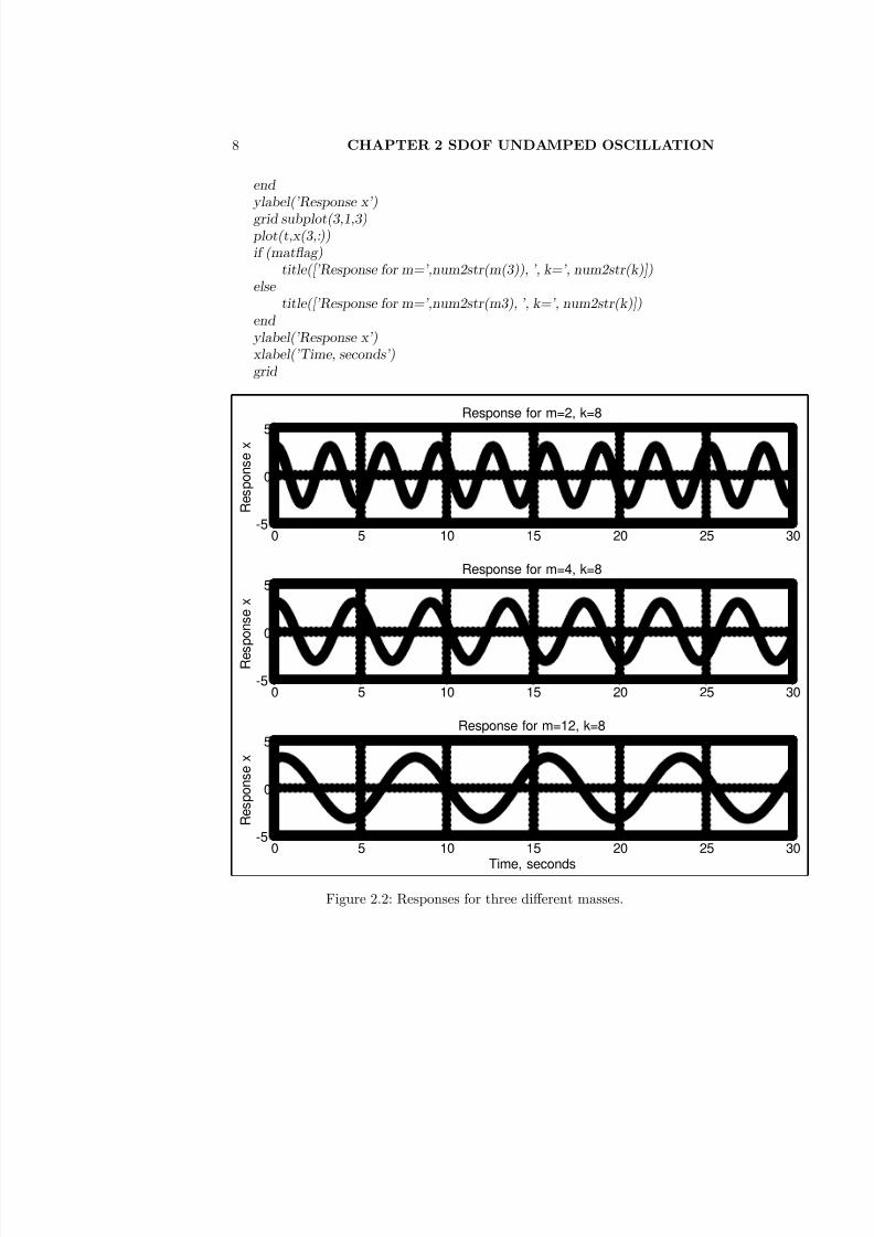
sti¤ness, then, will cause a variation in the frequency of vibration. The graphson the following pages demonstrate these sensitivities. Figure 2.2 shows thevariation of the vibrational characteristics for an increasing mass while sti¤nessremains constant. Figure 2.3 shows how the oscillatory behavior changes forincreasing sti¤ness with mass constant. For both Figures 2.2 and 2.3, the initialvelocity used was _xo = 1, and the initial displacement x0 = 3. Note that thefrequency decreases with increasing mass, but increases with increasing sti¤ness,as expected.
Looking at Equation 2.3, it is evident that the phase angle and maximumamplitude are also functions of the natural frequency. Again, referring to Figure
2.2, the maximum amplitude decreases with increasing mass, due to the corre-sponding reduction in natural frequency. As a result, the phase shift diminishes,with the peak of oscillation becoming nearer to t = 0. Note that the maximumdisplacement would occur at t = 0 if the initial velocity were zero. It is easilyveri…ed that, for this case, the parameter A (from Equation 2.2, above) reducesto xo, and the phase angle becomes tan1(0=x2
o), or 0.
In Figure 2.3, the maximum amplitude increases with increasing sti¤ness,due to the increase in natural frequency. The phase angle also increases withthe sti¤ness, so the maximum amplitude of oscillation occurs at an increasinglylater time with increasing sti¤ness.
The MATLAB code used to produce the graphs follows. The input state-ments in the …rst few lines demonstrate one type of interactive programming
available in MATLAB. The portion of the statement inside the quotation markswill appear on the screen when the program is run, so user prompts are easilyadded and explained. The initialization and use of the mass matrix is demon-strated in two ways. If the variable matflag is set to zero, then the masses areeach given scalar values. If this ‡ag is set to one, then the masses are initializedas part of an array. This is done to demonstrate the use of MATLAB array

8/20/2019 Vibrations Using Matlab
http://slidepdf.com/reader/full/vibrations-using-matlab 10/170
5
variables and to show how they can help streamline your code. Note also thatthe if..then structure in MATLAB is similar to that of Fortran in that these
statements must be closed with an end statement, as must any other loop (foror do, for example). We also demonstrate MATLAB’s plotting routines via thesubplot command, allowing plots for all three masses to be placed on the sameaxes. The second …gure below was produced by modifying the code below totake three sti¤nesses and one mass. The modi…cations necessary are left as anexercise for the reader.
Finally, those unfamiliar with MATLAB are probably wondering what allthe semicolons are after each line. By default, MATLAB prints the resultsof each operation to the screen. However, placing a semicolon at the end of a line suppresses this output. Since printing to screen takes time and mem-ory for MATLAB to perform, suppressing screen output of intermediate resultsincreases computational speed. (The reader is invited to remove all the semi-colons from the program to see the di¤erence!) This feature is also a very usefuldebugging tool. Instead of inserting and removing print statements to checkintermediate calculations, the programmer can insert and delete semicolons.

8/20/2019 Vibrations Using Matlab
http://slidepdf.com/reader/full/vibrations-using-matlab 11/170
8/20/2019 Vibrations Using Matlab
http://slidepdf.com/reader/full/vibrations-using-matlab 12/170
7
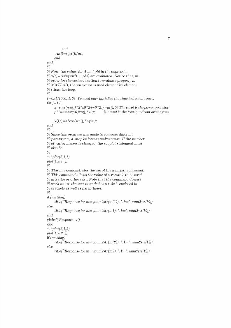
end wn(i)=sqrt(k/m);
end end %% Now, the values for A and phi in the expression% x(t)=Asin(wn*t + phi) are evaluated. Notice that, in% order for the cosine function to evaluate properly in% MATLAB, the wn vector is used element by element% (thus, the loop).%t=0:tf/1000:tf; % We need only initialize the time increment once.for j=1:3
a=sqrt(wn(j)^2*x0^2+v0^2)/wn(j); % The caret is the power operator. phi=atan2(v0,wn(j)*x0); % atan2 is the four-quadrant arctangent.
x(j,:)=a*cos(wn(j)*t-phi);end %% Since this program was made to compare di¤erent% parameters, a subplot format makes sense. If the number % of varied masses is changed, the subplot statement must% also be.%subplot(3,1,1)
plot(t,x(1,:))%
% This line demonstrates the use of the num2str command.% This command allows the value of a variable to be used % in a title or other text. Note that the command doesn’t% work unless the text intended as a title is enclosed in% brackets as well as parentheses.%if (mat‡ag)
title([’Response for m=’,num2str(m(1)), ’, k=’, num2str(k)])else
title([’Response for m=’,num2str(m1), ’, k=’, num2str(k)])end
ylabel(’Response x’)grid
subplot(3,1,2) plot(t,x(2,:))if (mat‡ag)
title([’Response for m=’,num2str(m(2)), ’, k=’, num2str(k)])else
title([’Response for m=’,num2str(m2), ’, k=’, num2str(k)])
8/20/2019 Vibrations Using Matlab
http://slidepdf.com/reader/full/vibrations-using-matlab 13/170
8 CHAPTER 2 SDOF UNDAMPED OSCILLATION
end ylabel(’Response x’)
grid subplot(3,1,3) plot(t,x(3,:))if (mat‡ag)
title([’Response for m=’,num2str(m(3)), ’, k=’, num2str(k)])else
title([’Response for m=’,num2str(m3), ’, k=’, num2str(k)])end
ylabel(’Response x’)xlabel(’Time, seconds’)grid
0 5 10 15 20 25 30-5
0
5
Response for m=2, k=8
R e s p o n s e x
0 5 10 15 20 25 30-5
0
5
Response for m=4, k=8
R e s
p o n s e x
0 5 10 15 20 25 30-5
0
5
Response for m=12, k=8
R e s p o n s e x
Time, seconds
Figure 2.2: Responses for three di¤erent masses.

8/20/2019 Vibrations Using Matlab
http://slidepdf.com/reader/full/vibrations-using-matlab 14/170
9
0 5 10 15 20 25 30-5
0
5
Response for m=5, k=2
R e s p o n s e x
0 5 10 15 20 25 30-5
0
5
Response for m=5, k=6
R e s p o n s e x
0 5 10 15 20 25 30-5
0
5
Response for m=5, k=13
R e s p o n s e x
Time, seconds
Figure 2.3: Responses for three di¤erent sti¤nesses.

8/20/2019 Vibrations Using Matlab
http://slidepdf.com/reader/full/vibrations-using-matlab 15/170

8/20/2019 Vibrations Using Matlab
http://slidepdf.com/reader/full/vibrations-using-matlab 16/170
Chapter 3
A Damped SDOF System
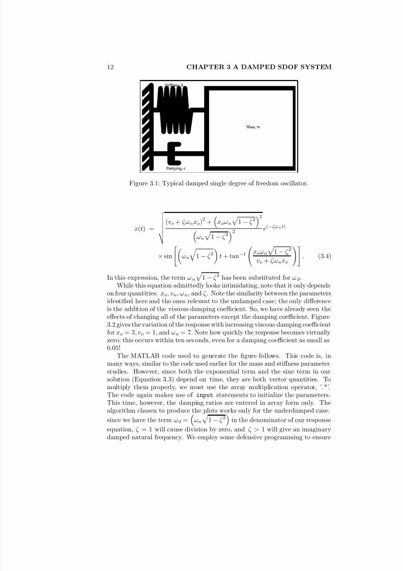
In the previous example, we examined the response of an undamped singledegree of freedom oscillator subject to varied mass and sti¤ness parameters.Here we will do the same for a damped single degree of freedom system.
Again, we begin with the equation of motion, given the system of Figure 3.1.A simple static analysis …nds that our equation is:
m::x + c
:x + k x = 0: (3.1)
If we divide through by m, we introduce the dimensionless parameters ! and :
::x + 2!n
:x + !2
n x = 0: (3.2)
In the above, !n represents the undamped natural frequency, and is theviscous damping ratio. For the purposes of this example, we will assume theunderdamped case ( < 1). The solution to this equation is:
x(t) = Ae!nt sin(!dt + ): (3.3)
In Equation 3.3, !d is the damped natural frequency, equal to !np
1 2
.
This equation is more useful if we write all of the terms as functions of parameters !n and :
11
8/20/2019 Vibrations Using Matlab
http://slidepdf.com/reader/full/vibrations-using-matlab 17/170
12 CHAPTER 3 A DAMPED SDOF SYSTEM
Figure 3.1: Typical damped single degree of freedom oscillator.
x(t) =
v uuuut (vo + !nxo)2 +
xo!n
p 1 22
!n
p 1 22 e(!nt)
sin
"!n
q 1 2
t + tan1
xo!n
p 1 2
vo + !nxo
!#: (3.4)
In this expression, the term !n
p 1 2 has been substituted for !d.
While this equation admittedly looks intimidating, note that it only dependson four quantities: xo, vo, !n, and . Note the similarity between the parameters
identi…ed here and the ones relevant to the undamped case; the only di¤erenceis the addition of the viscous damping coe¢cient. So, we have already seen thee¤ects of changing all of the parameters except the damping coe¢cient. Figure3.2 gives the variation of the response with increasing viscous damping coe¢cientfor xo = 3; vo = 1; and !n = 7. Note how quickly the response becomes virtuallyzero; this occurs within ten seconds, even for a damping coe¢cient as small as0.05!
The MATLAB code used to generate the …gure follows. This code is, inmany ways, similar to the code used earlier for the mass and sti¤ness parameterstudies. However, since both the exponential term and the sine term in oursolution (Equation 3.3) depend on time, they are both vector quantities. Tomultiply them properly, we must use the array multiplication operator, ’.*’.The code again makes use of input statements to initialize the parameters.This time, however, the damping ratios are entered in array form only. Thealgorithm chosen to produce the plots works only for the underdamped case;
since we have the term !d =
!n
p 1 2
in the denominator of our response
equation, = 1 will cause division by zero, and > 1 will give an imaginarydamped natural frequency. We employ some defensive programming to ensure

8/20/2019 Vibrations Using Matlab
http://slidepdf.com/reader/full/vibrations-using-matlab 18/170
13
allowable values for the damping ratio are entered. Conveniently, this gives us areason to introduce the while loop, analogous to the “do while” loop in Fortran.
The code checks each value zeta(zi) to see if it lies between zero and one. If not, a somewhat abrupt reminder is sent to the screen, and the loop asks for anew entry. Otherwise, it continues to the next damping ratio value. The logicaland relational operators in MATLAB are for the most part intuitive. Thus,if a>0 simply means “if a is greater than zero.” A full list can be found bytyping help ops at the MATLAB prompt; we will explain the ones we use incomments.

8/20/2019 Vibrations Using Matlab
http://slidepdf.com/reader/full/vibrations-using-matlab 19/170
14 CHAPTER 3 A DAMPED SDOF SYSTEM
Program 2-1: varyzeta.m%Initial value entry.
%The while loop in the zeta initialization section prevents %certain values for zeta from being entered, since such%values would crash the program.%wn=input(’Enter the natural frequency. ’);x0=input(’Enter the initial displacement. ’);v0=input(’Enter the initial velocity. ’);tf=input(’Enter the time duration to test, in seconds. ’);for zi=1:3
zeta(zi)=12;while(zeta(zi)<0 j zeta(zi)>=1) % The pipe ( j) means “or”.
zeta(zi)=input([’Enter damping coe¢cient value ’, num2str(zi),’.’]);
if (zeta(zi)>=1 j zeta(zi)<0)fprintf(’Zeta must be between 0 and 1!’);zeta(zi)=12;
end end
end %%Now, having !n and , the !d values can be found.%for i=1:3
wd(i)=wn*sqrt(1-zeta(i)^2);end
%%Solving for the response. Note the use of the array %multiplication command (.*) in the expression for x(t).%This command is necessary, else the program gives a %multiplication error.%t=0:tf/1000:tf;for j=1:3
a=sqrt((wn*x0*zeta(j)+v0)^2+(x0*wd(j))^2)/wd(j); phi=atan2(wd(j)*x0,v0+zeta(j)*wn*x0);x(j,:)=a*exp(-zeta(j)*wn*t).*sin(wd(j)*t+phi);
end %
%Now, the program plots the results in a subplot format.%subplot(3,1,1)
plot(t,x(1,:))title([’Response for zeta=’,num2str(zeta(1))])
ylabel(’Response x’)

8/20/2019 Vibrations Using Matlab
http://slidepdf.com/reader/full/vibrations-using-matlab 20/170
15
grid subplot(3,1,2)
plot(t,x(2,:))title([’Response for zeta=’, num2str(zeta(2))])
ylabel(’Response x’)grid subplot(3,1,3)
plot(t,x(3,:))title([’Response for zeta=’, num2str(zeta(3))])
ylabel(’Response x’)xlabel(’Time, seconds’)grid

8/20/2019 Vibrations Using Matlab
http://slidepdf.com/reader/full/vibrations-using-matlab 21/170
16 CHAPTER 3 A DAMPED SDOF SYSTEM
0 1 2 3 4 5 6 7 8 9 10-5
0
5
Response for zeta=0.05
R e s p o n s e x
0 1 2 3 4 5 6 7 8 9 10
-2
0
2
4Response for zeta=0.2
R e s p o n s e x
0 1 2 3 4 5 6 7 8 9 10-2
0
2
4Response for zeta=0.5
R e s p o n s e x
Time, seconds
Figure 3.2: Responses for various zeta values.
8/20/2019 Vibrations Using Matlab
http://slidepdf.com/reader/full/vibrations-using-matlab 22/170
Chapter 4
Overdamped SDOF
Oscillation
The previous example is valid only for the underdamped case, < 1. But whathappens when this condition is not met? There are two cases to explore: > 1(the overdamped case), and = 1 (the critically damped case). First, we needto see how these cases arise in order to understand what the results will be. Theequation of motion of a damped single degree of freedom oscillator is:
::x + 2!n
:x + !2
nx = 0: (4.1)
Assume a solution of the form Aet, substitute it appropriately into Equation
4.1, and obtain the quadratic formula de…ning possible values for :
= !n !n
q 2 1: (4.2)
Note that the quantity inside the radical is always greater than zero, sincewe have assumed > 1. Therefore, the solution of the equation of motion is
x(t) = e!nt(a1e!ntp
21 + a2e!ntp
21): (4.3)
If we again take our initial displacement as xo and initial velocity vo, the
constants a1; a2 become
a1 = vo + ( +
p 2 1)!nxo
2!n
p 2 1
; a2 = vo + ( +
p 2 1)!nxo
2!n
p 2 1
: (4.4)
17

8/20/2019 Vibrations Using Matlab
http://slidepdf.com/reader/full/vibrations-using-matlab 23/170
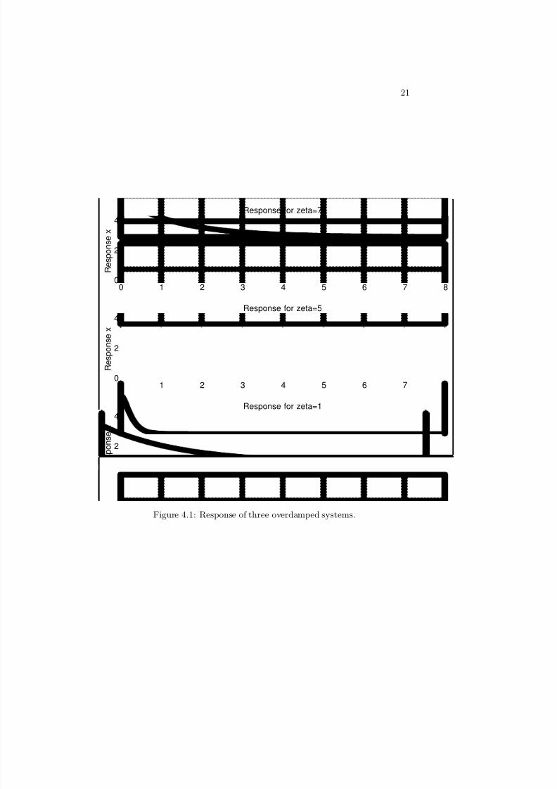
18 CHAPTER 4 OVERDAMPED SDOF OSCILLATION
Equation 4.3 is a decaying exponential and the system will simply return toits initial position instead of oscillating about the equilibrium. This is shown
in Figure 4.1. Note that if = 1, a singularity exists in the constants; asecond independent solution must be found. From our knowledge of ordinarydi¤erential equations, we can …nd
x(t) = (a1 + a2t)e!nt; (4.5)
where a1 = xo; and a2 = vo + !nxo.Figure 4.1 was generated for !n = 7; xo = 3; and o = 1. Notice how the
critically damped response returns to equilibrium faster than the others. Forthe plots in the …gure, the motion with critical damping is stopped after abouttwo seconds, while the others do not reach equilibrium until more than eightseconds. This is the distinguishing characteristic of the critically damped case.Note also that the motion of the masses is, as expected, purely exponential;
there is no oscillation, only a decay of the response to equilibrium.The MATLAB code is again presented below. The astute reader may ask
why the codes for underdamped, critically damped, and overdamped vibrationcould not be combined into a single code. Certainly they can be; the modi…-cations are left to the reader. The resulting code should reject negative valuesfor the damping ratio. (Hint: You may …nd the switch command to be useful,especially when used with its otherwise case.)
8/20/2019 Vibrations Using Matlab
http://slidepdf.com/reader/full/vibrations-using-matlab 24/170
19
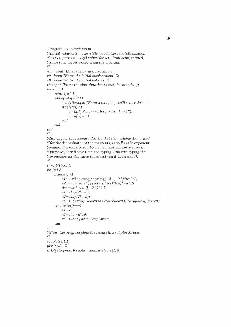
Program 3-1: overdamp.m%Initial value entry. The while loop in the zeta initialization
%section prevents illegal values for zeta from being entered,%since such values would crash the program.%wn=input(’Enter the natural frequency. ’);x0=input(’Enter the initial displacement. ’);v0=input(’Enter the initial velocity. ’);tf=input(’Enter the time duration to test, in seconds. ’);for zi=1:3
zeta(zi)=0.12;while(zeta(zi)<1)
zeta(zi)=input(’Enter a damping coe¢cient value. ’);if zeta(zi)<1
fprintf(’Zeta must be greater than 1!’);zeta(zi)=0.12;
end end
end %%Solving for the response. Notice that the variable den is used %for the denominator of the constants, as well as the exponent%values. If a variable can be created that will serve several %purposes, it will save time and typing. (imagine typing the %expression for den three times and you’ll understand).%t=0:tf/1000:tf;
for j=1:3 if zeta(j)>1a1n=-v0+(-zeta(j)+(zeta(j)^2-1)^0.5)*wn*x0;a2n=v0+(zeta(j)+(zeta(j)^2-1)^0.5)*wn*x0;den=wn*(zeta(j)^2-1)^0.5;a1=a1n/(2*den);a2=a2n/(2*den);x(j,:)=(a1*exp(-den*t)+a2*exp(den*t)).*exp(-zeta(j)*wn*t);
elseif zeta(j)==1a1=x0;a2=v0+wn*x0;x(j,:)=(a1+a2*t).*exp(-wn*t);
end
end %Now, the program plots the results in a subplot format.%subplot(3,1,1)
plot(t,x(1,:))title([’Response for zeta=’,num2str(zeta(1))])

8/20/2019 Vibrations Using Matlab
http://slidepdf.com/reader/full/vibrations-using-matlab 25/170
20 CHAPTER 4 OVERDAMPED SDOF OSCILLATION
ylabel(’Response x’)grid
subplot(3,1,2) plot(t,x(2,:))title([’Response for zeta=’, num2str(zeta(2))])
ylabel(’Response x’)grid subplot(3,1,3)
plot(t,x(3,:))title([’Response for zeta=’, num2str(zeta(3))])
ylabel(’Response x’)xlabel(’Time, seconds’)grid
8/20/2019 Vibrations Using Matlab
http://slidepdf.com/reader/full/vibrations-using-matlab 26/170
21
0 1 2 3 4 5 6 7 80
2
4
Response for zeta=7
R e s p o n s e x
0 1 2 3 4 5 6 7 80
2
4
Response for zeta=5
R e s p o n s e x
0 1 2 3 4 5 6 7 80
2
4
Response for zeta=1
R e s p o n s e x
Time, seconds
Figure 4.1: Response of three overdamped systems.

8/20/2019 Vibrations Using Matlab
http://slidepdf.com/reader/full/vibrations-using-matlab 27/170
8/20/2019 Vibrations Using Matlab
http://slidepdf.com/reader/full/vibrations-using-matlab 28/170
Chapter 5
Harmonic Excitation of
Undamped SDOF Systems
In the previous examples, we examined the responses of single degree of freedomsystems which were not subjected to an external force. Now, we will examinethe e¤ects of an external force on the system. We begin with the simplest formof external forcing: the harmonic load.
The system under consideration is shown in Figure 5.1. The forcing functionis assumed to be of the form F (t) = F o cos !t, where ! is the driving frequency.For the case with no damping, Newton’s Second Law gives us the equation of motion m
::x + kx = F o cos !t; or
::x + !2nx = f o cos !t; (5.1)
where f o = F o=m. We know the solution for the response x(t) to be:
x(t) = A1 sin !nt + A2 cos !nt + f o
!2n !2
cos !t; (5.2)
where
A1 =
vo
!n ; A2 = xo f o
!2n !2 : (5.3)
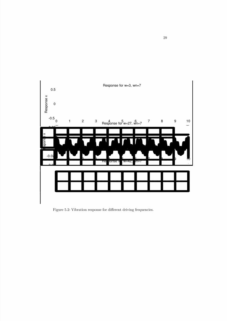
The key parameters which de…ne the response are the natural and drivingfrequencies, or more precisely, their ratio !=!n: Figure 5.2 shows the e¤ect of varying driving frequency ! for a given natural frequency, and Figure 5.3 does
23

8/20/2019 Vibrations Using Matlab
http://slidepdf.com/reader/full/vibrations-using-matlab 29/170

8/20/2019 Vibrations Using Matlab
http://slidepdf.com/reader/full/vibrations-using-matlab 30/170
25
The MATLAB code below uses the subplot command more elegantly thanwe had in earlier examples. Instead of typing out three separate sets of plotting
commands, the subplots are done in a loop. A simple (and natural) modi…cationto this program would be to change the number of plots in the subplot. Thiscould be done by introducing an integer variable nplot and changing the loopsto run from one to nplot instead of one to three. From a practical point of view, though, introducing too many plots to the …gures would make the plotunreadable, so care must be taken. Also, we’ve changed the parameter valuesfrom dynamic inputs to static values. They can easily be changed back to userinputs.

8/20/2019 Vibrations Using Matlab
http://slidepdf.com/reader/full/vibrations-using-matlab 31/170
26CHAPTER 5 HARMONIC EXCITATION OF UNDAMPED SDOF SYSTEMS
Program 4-1 - varywdr.m%This program is very straightforward. The program takes
%the necessary input values to solve Equation%5.3 for three di¤erent driving %frequencies, checks for resonance (since we don’t want to %handle that problem yet), and plots.%%This …le varies driving frequency of a single degree %of freedom undamped oscillator at a set natural %frequency. The initial displacement is 3, the velocity is %1, the force magnitude per unit mass is 6, and the %natural frequency is 7.wn=7;x0=0;v0=0;f0=6;tf=10;wdr=zeros(3,1);x=zeros(3,1001);for i=1:3;
wdr(i)=wn; % This is how we initialize our while loop.while wdr(i)==wn;
wdr(i)=input(’Enter the driving frequency. ’);if wdr(i)==wn;
fprintf(’This will produce resonance!!’)end
end
end t=0:tf/1000:tf;for j=1:3
A1=v0/wn;A2=x0-(f0/(wn^2-wdr(j)^2));A3=f0/(wn^2-wdr(j)^2);x(j,:)=A1*sin(wn*t)+A2*cos(wn*t)+A3*cos(wdr(j)*t);
end for k=1:3 % We could have used subplot this way all along.
subplot(3,1,k) plot(t,x(k,:))title([’Response for wdr=’,num2str(wdr(k)),’,wn=’,num2str(wn)])
ylabel(’Response x’)grid
end xlabel(’Time, seconds’)

8/20/2019 Vibrations Using Matlab
http://slidepdf.com/reader/full/vibrations-using-matlab 32/170
27
Program 4-2: varywn.m%This program is similar in form to varywdr.m, except that
%now the natural frequency is the variable.%%This …le varies natural frequency of a single degree %of freedom undamped oscillator at a set driving %frequency. The initial displacement is 3, the velocity is %1, the force magnitude per unit mass is 6, and the %driving frequency is 7.wdr=7;x0=0;v0=0;f0=6;tf=10;wn=zeros(3,1);x=zeros(3,1001);for i=1:3;
wn(i)=wdr; % Analagous to the initialization above.while wn(i)==wdr;
wn(i)=input(’Enter the natural frequency. ’);if wn(i)==wdr;
fprintf(’This will produce resonance!!’)end
end end t=0:tf/1000:tf;for j=1:3
A1=v0/wn(j);A2=x0-(f0/(wn(j)^2-wdr^2));A3=f0/(wn(j)^2-wdr^2);x(j,:)=A1*sin(wn(j)*t)+A2*cos(wn(j)*t)+A3*cos(wdr*t);
end for k=1:3
subplot(3,1,k) plot(t,x(k,:))title([’Response for wdr=’,num2str(wdr),’,wn=’,num2str(wn(k))])
ylabel(’Response x’)grid
end
xlabel(’Time, seconds’)

8/20/2019 Vibrations Using Matlab
http://slidepdf.com/reader/full/vibrations-using-matlab 33/170
28CHAPTER 5 HARMONIC EXCITATION OF UNDAMPED SDOF SYSTEMS
Program 4-3: beatres.m%The main feature of note for this code is the use of the
%if-then-else protocol in MATLAB to allow solutions other %than “Inf” for the resonant case. By changing the values %of the initial conditions, wn, and f0 to input%statements, this program would become a general solver %for the single-degree of freedom undamped oscillator,%subject to harmonic forcing.%%This program shows beats and resonance in undamped %systems. Again, in order to better see the e¤ects, the %initial velocity and displacement are zero.x0=0;v0=0;wn=3;wdr=input(’Enter the driving frequency. ’);f0=6;tf=120;%This section chooses the proper response formula for %the given situation.t=0:tf/1000:tf;if wdr==wn
A1=v0/wn;A2=x0;A3=f0/2*wn;x=A1*sin(wn*t)+A2*cos(wn*t)+A3*t.*cos(wdr*t);
else
A1=v0/wn;A2=x0-(f0/(wn^2-wdr^2));A3=f0/(wn^2-wdr^2);x=A1*sin(wn*t)+A2*cos(wn*t)+A3*cos(wdr*t);
end plot(t,x);if wdr==wn
title(’Example of Resonance Phenomenon’);else
title(’Example of Beat Phenomenon’);end xlabel(’Time, seconds’)
ylabel(’Response x’)
grid
8/20/2019 Vibrations Using Matlab
http://slidepdf.com/reader/full/vibrations-using-matlab 34/170
29
0 1 2 3 4 5 6 7 8 9 10-0.5
0
0.5
Response for w=3, wn=7
R
e s p o n s e x
0 1 2 3 4 5 6 7 8 9 10-0.02
0
0.02Response for w=27, wn=7
R e s p o n s e x
0 1 2 3 4 5 6 7 8 9 10-0.01
0
0.01
Response for w=42, wn=7
R e s p o n s e x
Time, seconds
Figure 5.2: Vibration response for di¤erent driving frequencies.

8/20/2019 Vibrations Using Matlab
http://slidepdf.com/reader/full/vibrations-using-matlab 35/170
30CHAPTER 5 HARMONIC EXCITATION OF UNDAMPED SDOF SYSTEMS
0 1 2 3 4 5 6 7 8 9 10-0.5
0
0.5
Response for w=7, wn=3
R
e s p o n s e x
0 1 2 3 4 5 6 7 8 9 10-0.2
0
0.2Response for w=7, wn=12
R e s p o n s e x
0 1 2 3 4 5 6 7 8 9 10-0.02
0
0.02
Response for w=7, wn=26
R e s p o n s e
x
Time, seconds
Figure 5.3: Vibration response for di¤erent natural frequencies.

8/20/2019 Vibrations Using Matlab
http://slidepdf.com/reader/full/vibrations-using-matlab 36/170
31
0 20 40 60 80 100 120-25
-20
-15
-10
-5
0
5
10
15
20
25
Example of Beat Phenomenon
Time, seconds
R e s p o n s e x
Figure 5.4: Example of the beating phenomenon.

8/20/2019 Vibrations Using Matlab
http://slidepdf.com/reader/full/vibrations-using-matlab 37/170
32CHAPTER 5 HARMONIC EXCITATION OF UNDAMPED SDOF SYSTEMS
0 20 40 60 80 100 120-1500
-1000
-500
0
500
1000
1500
Example of Resonance Phenomenon
Time, seconds
R e s p o n s e
x
Figure 5.5: Example of resonant vibration.

8/20/2019 Vibrations Using Matlab
http://slidepdf.com/reader/full/vibrations-using-matlab 38/170
Chapter 6
Harmonic Forcing of
Damped SDOF Systems
Now, we will examine how the behavior of the system changes when we adddamping. As with the unforced case, the equations of motion change whendamping is added. They become:
m•x + c _x + kx = F cos(!t); (6.1)
or with = c=2m!n;
•x + 2!n _x + !2nx = f cos(!t); (6.2)
where f = F =m. The homogeneous solution to this equation is of the form
xh(t) = Ae!t sin(!dt + ); (6.3)
where !d = !n
p 1 2; and constants A; depend on initial conditions. The
particular solution to the external force is
x p(t) = A0 cos(!t ); (6.4)
where
A0 = f q
(!2n !2) + (2!n!)2
; = tan1 2!n!
!2n !2
: (6.5)
33

8/20/2019 Vibrations Using Matlab
http://slidepdf.com/reader/full/vibrations-using-matlab 39/170
34CHAPTER 6 HARMONIC FORCING OF DAMPED SDOF SYSTEMS
The complete solution, x(t) = xh(t)+x p(t) is then used to evaluate constantsA and . These constants were found for zero initial conditions using Maple;
this solution is re‡ected in the code that follows.The addition of damping causes the response of the system to di¤er slightly,
as shown in Figures 6.1 and 6.2. In Figure 6.1, the damping ratio was varied.This shows that the transient period of vibration varies inversely with dampingratio. The length of the transient period varies from about 4.5 seconds for =0:05 to about 2 seconds for = 0:3; showing that, in many cases, the transientresponse can be ignored due to its short time period. However, for some cases,the transient period may be much longer or may have a very large amplitude,so it is always important to examine the transient e¤ects of a system beforeneglecting them. Notice also that the damping ratio a¤ects the amplitude of the steady-state vibration, also in an inverse relationship. That is, the amplitudeof the response for = 0:05 is almost 2, while that for = 0:3 is less than 1.
Figure 6.2 shows the e¤ects of changing the natural frequency. Notice how,for the two frequencies that are near the driving frequency, the transient periodis quite long, almost 10 seconds. However, for the large natural frequency,the transient period is less than 4 seconds, which shows that the length of thetransient period also depends on the natural frequency.
In the damped system, resonance also takes on a di¤erent meaning. Noticehow, for ! = !n; the amplitude does not become in…nite; the introductionof damping introduces a term that keeps the denominator of the steady-stateamplitude from becoming zero. However, at this point, the phase angle becomes90: For a damped system, this condition de…nes resonance, since it is also atthis point that the denominator of the amplitude is a minimum. To prove thislast assertion to yourself, look at the denominator of the amplitude constant,A0: The amplitude will be maximized when the denominator is minimized. Both
terms are never negative, so the minimum will occur when the two frequenciesare equal (making the …rst term of the denominator zero). Also, as the drivingfrequency increases greatly, the amplitude nears zero.
The MATLAB code below was used to produce the …gures. Instead of insert-ing a while statement to control the range of damping ratios used, we use an if
statement, in tandem with an error statement. If the damping ratio is outsidethe allowed range, MATLAB will halt execution of the program, printing thestatement found inside the quotation marks to the screen. Controlling input inthis manner is more drastic than the method used in the previous programs.However, those programs had many more values to input. Forcing the user of a program to reenter several values because of a typo seems a harsh penalty tothis programmer. Also, this program introduces MATLAB’s method for con-tinuing lines. To continue an expression onto the next line, simply type three
periods in succession (ellipsis) and move to the next line. This is helpful for longmathematical expressions, like the constants of integration below. This ellipsiscan be placed anywhere a space would be allowed, so continuing in the middleof a variable name, for example, is not recommended.
8/20/2019 Vibrations Using Matlab
http://slidepdf.com/reader/full/vibrations-using-matlab 40/170
35
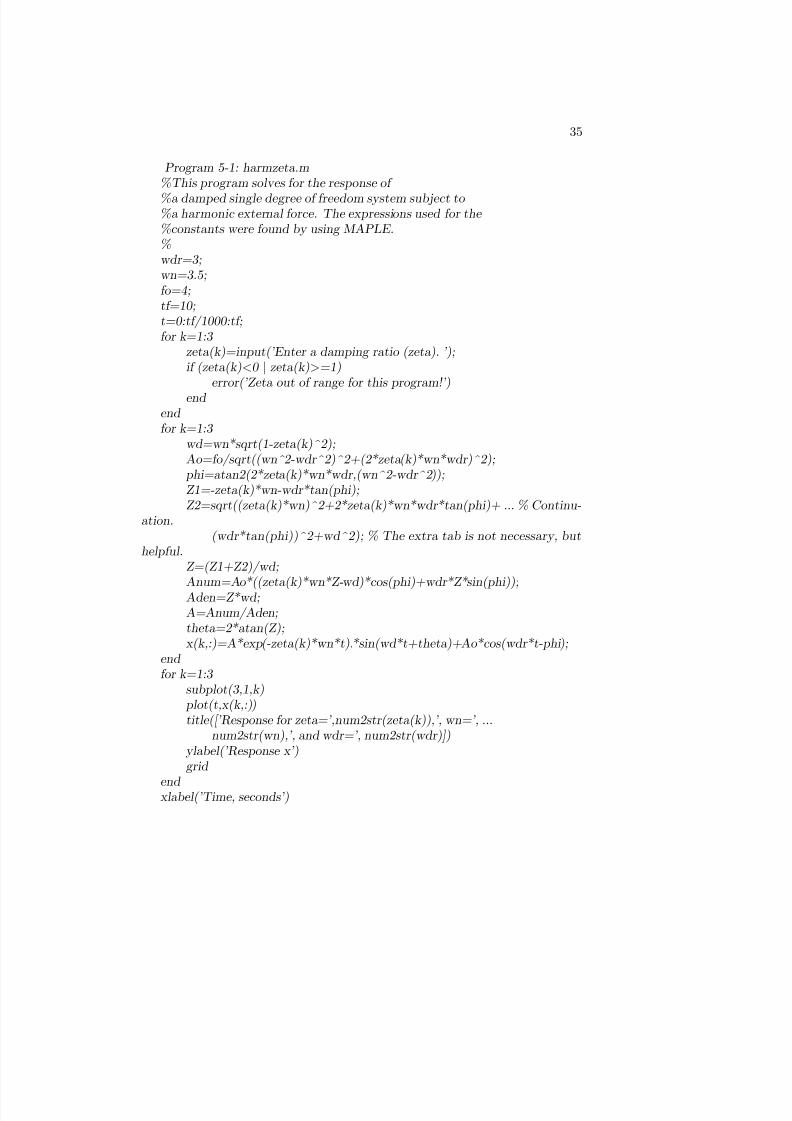
Program 5-1: harmzeta.m%This program solves for the response of
%a damped single degree of freedom system subject to %a harmonic external force. The expressions used for the %constants were found by using MAPLE.%wdr=3;wn=3.5;fo=4;tf=10;t=0:tf/1000:tf;for k=1:3
zeta(k)=input(’Enter a damping ratio (zeta). ’);if (zeta(k)<0 j zeta(k)>=1)
error(’Zeta out of range for this program!’)end
end for k=1:3
wd=wn*sqrt(1-zeta(k)^2);Ao=fo/sqrt((wn 2̂-wdr^2)^2+(2*zeta(k)*wn*wdr)^2);
phi=atan2(2*zeta(k)*wn*wdr,(wn^2-wdr^2));Z1=-zeta(k)*wn-wdr*tan(phi);Z2=sqrt((zeta(k)*wn)^2+2*zeta(k)*wn*wdr*tan(phi)+ ... % Continu-
ation.(wdr*tan(phi))^2+wd^2); % The extra tab is not necessary, but
helpful.Z=(Z1+Z2)/wd;
Anum=Ao*((zeta(k)*wn*Z-wd)*cos(phi)+wdr*Z*sin(phi));Aden=Z*wd;A=Anum/Aden;theta=2*atan(Z);x(k,:)=A*exp(-zeta(k)*wn*t).*sin(wd*t+theta)+Ao*cos(wdr*t-phi);
end for k=1:3
subplot(3,1,k) plot(t,x(k,:))title([’Response for zeta=’,num2str(zeta(k)),’, wn=’, ...
num2str(wn),’, and wdr=’, num2str(wdr)]) ylabel(’Response x’)grid
end xlabel(’Time, seconds’)

8/20/2019 Vibrations Using Matlab
http://slidepdf.com/reader/full/vibrations-using-matlab 41/170
36CHAPTER 6 HARMONIC FORCING OF DAMPED SDOF SYSTEMS
0 1 2 3 4 5 6 7 8 9 10-2
0
2
Response for zeta=0.05, wn=3.5, and w=3
R e s p o n s e x
0 1 2 3 4 5 6 7 8 9 10-2
0
2
Response for zeta=0.1, wn=3.5, and w=3
R e s p o n s e x
0 1 2 3 4 5 6 7 8 9 10-1
0
1
Response for zeta=0.3, wn=3.5, and w=3
R e s p o n s e x
Time, seconds
Figure 6.1: Damped response for three di¤erent damping ratios.

8/20/2019 Vibrations Using Matlab
http://slidepdf.com/reader/full/vibrations-using-matlab 42/170
37
0 1 2 3 4 5 6 7 8 9 10-2
0
2
Response for zeta=0.05, wn=2, and w=3
R
e s p o n s e x
0 1 2 3 4 5 6 7 8 9 10-1
0
1Response for zeta=0.05, wn=4, and w=3
R e s p o n s e x
0 1 2 3 4 5 6 7 8 9 10-0.05
0
0.05
Response for zeta=0.05, wn=16, and w=3
R e s p o n s e x
Time, seconds
Figure 6.2: Response variation with di¤erent natural frequencies.

8/20/2019 Vibrations Using Matlab
http://slidepdf.com/reader/full/vibrations-using-matlab 43/170
8/20/2019 Vibrations Using Matlab
http://slidepdf.com/reader/full/vibrations-using-matlab 44/170
Chapter 7
Base Excitation of SDOF
Systems
The base excitation problem is illustrated in Figure 7.1. Let the motion of thebase be denoted by y(t) and the response of the mass by x(t), and assumingthat the base has harmonic motion of the form y(t) = Y sin(!bt). The equationof motion for this system is:
m::x + c(
:x :
y) + k(x y) = 0: (7.1)
Using the assumed form for the motion, we can substitute for y and its deriva-tive, resulting in:
m::x + c
:x + kx = cY !b cos !bt + kY sin !bt; (7.2)
which when divided through by the mass, yields
::x + 2!
:x + !2x = 2!!b cos !bt + !2Y sin !bt: (7.3)
The homogeneous solution is of the form:
xh = Ae!t sin(!dt + ): (7.4)
The expression for each part of the particular solution is similar to that forthe general sinusoidal forcing function; the sine term produces a sine solution,and the cosine term produces a cosine solution. If we …nd these solutions andcombine their sum into a single sinusoid, we obtain:
39

8/20/2019 Vibrations Using Matlab
http://slidepdf.com/reader/full/vibrations-using-matlab 45/170
40 CHAPTER 7 BASE EXCITATION OF SDOF SYSTEMS
Figure 7.1: Typical single degree of freedom system subject to base excitation.
x p = Ao cos(!bt 1 2); (7.5)
where
Ao = !Y
s !2 + (2!b)2
(!2 !2b)2 + (2!!b)2
; 1 = tan1 2! !b
!2 !2b
; 2 = tan1 !
2!b:
Thus, the complete solution is the sum of the homogeneous and particularsolutions, or:
x(t) = Ae!t sin(!dt + ) + Ao cos(!bt 1 2): (7.6)
This equation tells us a great deal about the motion of the mass. First, wecan see that the particular solution represents the steady-state response, whilethe homogeneous solution is the transient response, since the particular solutionis independent of the initial displacement and velocity. Using MAPLE to solvethe initial value problem (with given initial velocity and displacement not nec-essarily equal to zero), we …nd that both are dependent upon the initial velocity

8/20/2019 Vibrations Using Matlab
http://slidepdf.com/reader/full/vibrations-using-matlab 46/170
41
and displacement. However, the expression for the constants A and is, in gen-eral, very di¢cult to solve, even for MAPLE. So, for the sake of programming
in MATLAB, the initial velocity and displacement were both assumed to bezero. This assumption yielded simpler equations, which were used in the baseexcitation programs which follow.
Figure 7.2 shows the e¤ects of changing the excitation frequency while hold-ing all other parameters constant. In the steady state, from about three secondsforward, note that the frequency of vibration increases with the base frequency.This is expected, since the base excitation portion dominates the steady state.Of particular note is the bottom plot, with !b = 20: In the transient portion,the response has the shape of a sum of two sinusoids; these are, of course, thetransient and steady-state functions. Since the base excitation is of such highfrequency, this graph shows best what is happening between the transient andsteady responses. Note that, if a line was drawn through the upper or lowerpeaks of the motion, the result would be a curve similar to that exhibited bya damped free response. The midpoint of the oscillation caused by the steadyresponse becomes exponentially closer to zero with increasing time, as the tran-sient response diminishes.
Figure 7.3 gives plots for three di¤erent vibration amplitudes. The di¤er-ences caused by changing the amplitude is what would be expected; the maxi-mum amplitude of the overall vibration and of the steady-state response bothincrease with increasing input amplitude.
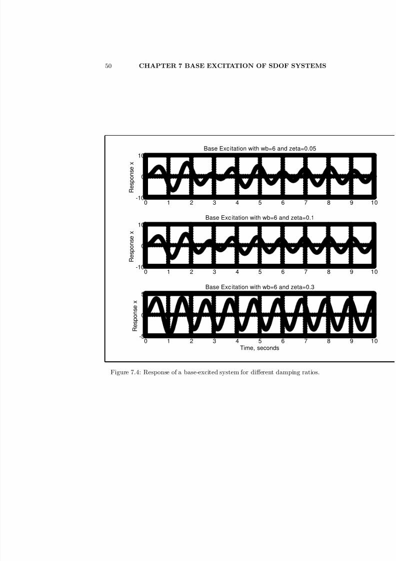
The plots in Figure 7.4 for various damping ratios show two e¤ects of chang-ing the damping ratio. First, the change in damping ratio causes the lengthof the transient period to vary; an increase in causes the transient period todecrease, as the plots show. Also, the change in damping ratio causes a changein the frequency of the transient vibration. Again, an increase in causes a
decrease in the damped natural frequency, although the decrease is not entirelyevident from just looking at the plots. This is because the plots also include thebase excitation (steady-state) terms, whose frequency has not changed.
The MATLAB code for this situation is much more complex than the codeused in previous examples. This is mainly due to the increased di¢culty en-countered when the external load is applied to a part of the structure. Whenthis approach is used, the relative displacement of the two parts of the struc-ture becomes the important factor, instead of the displacement of the structurerelative to some ground. The code for this example uses a solution obtainedfrom the MAPLE solve routine to produce a plot of the response. An impor-tant consideration to note is that the answer given by MAPLE results in twopossible solutions; the MATLAB code attempts to locate the correct one. Theway in which MATLAB chooses the correct solution is to check which of them
matches the initial displacement condition. Note from the plots that the initialdisplacements are zero for all plots, as are the initial velocities, so we can becon…dent in the plotted solutions. The three programs given below show thechanges that need to be made in a program in order to test di¤erent parameters.

8/20/2019 Vibrations Using Matlab
http://slidepdf.com/reader/full/vibrations-using-matlab 47/170
42 CHAPTER 7 BASE EXCITATION OF SDOF SYSTEMS
Program 6-1: varywb.m%This program solves the base excitation problem. The
%code assumes a sinusoidal base function. Also, the %program tests three di¤erent natural frequencies.%
y0=input(’Enter the base excitation magnitude. ’);zeta=input(’Enter the damping ratio (zeta). ’);if (zeta <0 j zeta >=1) % The usual test on damping ratio.
error(’Damping ratio not in acceptable range!’)end wn=4;tf=10;t=0:tf/1000:tf;for k=1:3
wb(k)=input(’Enter a base excitation frequency. ’);end for m=1:3 %%This section solves the transient response, using the %equations obtained from MAPLE.%
wd=wn*sqrt(1-zeta^2); phi1=atan2(2*zeta*wn*wb(m),(wn^2-wb(m)^2)); phi2=atan2(wn,2*zeta*wb(m));xi=phi1+phi2;
%These constants are what produces the two possible %solutions discussed above. Notice the way by which
%the extraordinarily long expressions for the constants %are broken into parts, to keep the expressions from%spreading over several lines.
Z1=(-zeta*wn-wb(m)*tan(xi)+sqrt((zeta*wn)^2+2*zeta* ...wn*wb(m)*tan(xi)+(wb(m)*tan(xi))^2+wd^2))/wd;
Z2=(-zeta*wn-wb(m)*tan(xi)-sqrt((zeta*wn)^2+2*zeta* ...wn*wb(m)*tan(xi)+(wb(m)*tan(xi))^2+wd^2))/wd;
Anum=sqrt((wn^2+(2*zeta*wb(m))^2)/((wn^2-wb(m)^2)^2+(2* ...zeta*wb(m)*wn)^2))*wn*y0;
Bnum1=(-wd*cos(xi)+Z1*zeta*wn*cos(xi)+Z1*wb(m)*sin(xi));Bnum2=(-wd*cos(xi)+Z2*zeta*wn*cos(xi)+Z2*wb(m)*sin(xi));Aden1=wd*Z1;Aden2=wd*Z2;
A1=Anum*Bnum1/Aden1;A2=Anum*Bnum2/Aden2;th1=2*atan(Z1);th2=2*atan(Z2);
y1(m,:)=A1*exp(-zeta*wn*t).*sin(wd*t+th1); y2(m,:)=A2*exp(-zeta*wn*t).*sin(wd*t+th2);

8/20/2019 Vibrations Using Matlab
http://slidepdf.com/reader/full/vibrations-using-matlab 48/170
43
end %This portion solves the steady-state response.
for j=1:3 A=sqrt((wn^2+(2*zeta*wb(j))^2)/((wn^2-wb(j)^2)^2+(2*zeta* ...wn*wb(j))^2));
phi1=atan2(2*zeta*wn*wb(j),(wn^2-wb(j)^2)); phi2=atan2(wn,(2*zeta*wb(j)));xp(j,:)=wn*y0*A*cos(wb(j)*t-phi1-phi2);
end if (xp(1,1)+y1(1,1)==xp(2,1)+y1(2,1)==xp(3,1)+y1(3,1)==0)
x=xp+y1;else
x=xp+y2;end for i=1:3
subplot(3,1,i) plot(t,x(i,:)) ylabel(’Response x’);title([’Base Excitation with wb=’,num2str(wb(i)), ...’ and wn=’,num2str(wn)]);grid
end xlabel(’Time, seconds’)

8/20/2019 Vibrations Using Matlab
http://slidepdf.com/reader/full/vibrations-using-matlab 49/170
44 CHAPTER 7 BASE EXCITATION OF SDOF SYSTEMS
Program 6-2: varyyobe.m%This program solves the base excitation problem. The
%code assumes a sinusoidal base function. Also, the %program tests three di¤erent base amplitudes.%Notice that the natural frequency is now given as %a set variable, and the variable ’y0’ is a user-input matrix.%wb=input(’Enter the base excitation frequency. ’);zeta=input(’Enter the damping ratio (zeta). ’);if (zeta <0 j zeta >=1) % The usual test on damping ratio.
error(’Damping ratio not in acceptable range!’)end wn=4;tf=10;t=0:tf/1000:tf;for k=1:3
y0(k)=input(’Enter a base excitation magnitude. ’);end for m=1:3
wd=wn*sqrt(1-zeta^2); phi1=atan2(2*zeta*wn*wb,(wn^2-wb^2)); phi2=atan2(wn,2*zeta*wb);xi=phi1+phi2;Z1=(-zeta*wn-wb*tan(xi)+sqrt((zeta*wn)^2+2*zeta* ...
wn*wb*tan(xi)+(wb*tan(xi))^2+wd^2))/wd;Z2=(-zeta*wn-wb*tan(xi)-sqrt((zeta*wn)^2+2*zeta* ...
wn*wb*tan(xi)+(wb*tan(xi))^2+wd^2))/wd;
Anum=sqrt((wn^2+(2*zeta*wb)̂ 2)/((wn^2-wb^2)^2+(2* ...zeta*wb*wn)^2))*wn*y0(m);Bnum1=(-wd*cos(xi)+Z1*zeta*wn*cos(xi)+Z1*wb*sin(xi));Bnum2=(-wd*cos(xi)+Z2*zeta*wn*cos(xi)+Z2*wb*sin(xi));Aden1=wd*Z1; Aden2=wd*Z2;A1=Anum*Bnum1/Aden1;A2=Anum*Bnum2/Aden2;th1=2*atan(Z1);th2=2*atan(Z2);
y1(m,:)=A1*exp(-zeta*wn*t).*sin(wd*t+th1); y2(m,:)=A2*exp(-zeta*wn*t).*sin(wd*t+th2);
end for j=1:3
A=sqrt((wn^2+(2*zeta*wb)^2)/((wn^2-wb^2)^2+(2*zeta* ...wn*wb)^2));
phi1=atan2(2*zeta*wn*wb,(wn^2-wb^2)); phi2=atan2(wn,(2*zeta*wb));xp(j,:)=wn*y0(j)*A*cos(wb*t-phi1-phi2);
end

8/20/2019 Vibrations Using Matlab
http://slidepdf.com/reader/full/vibrations-using-matlab 50/170
45
if (xp(1,1)+y1(1,1)==xp(2,1)+y1(2,1)==xp(3,1)+y1(3,1)==0)x=xp+y1;
else x=xp+y2;
end for i=1:3
subplot(3,1,i) plot(t,x(i,:)) ylabel(’Response x’);title([’Base Excitation with wb=’,num2str(wb), ...’, wn=’,num2str(wn),’, and y0=’,num2str(y0(i))]);grid
end xlabel(’Time, seconds’)

8/20/2019 Vibrations Using Matlab
http://slidepdf.com/reader/full/vibrations-using-matlab 51/170
46 CHAPTER 7 BASE EXCITATION OF SDOF SYSTEMS
Program 6-3: varyzbe.m%This program solves the base excitation problem. The
%code assumes a sinusoidal base function. Also, the %program tests three di¤erent damping ratios. Again, note %the changes between this program and the previous one.%
y0=input(’Enter the base excitation magnitude. ’);wb=input(’Enter the base excitation frequency. ’);wn=4;tf=10;t=0:tf/1000:tf;for k=1:3
zeta(k)=input(’Enter a damping ratio (zeta). ’);if (zeta(k)<0 j zeta(k)>=1) % The usual test on damping ratio.
error(’Damping ratio not in acceptable range!’)end
end for m=1:3
wd=wn*sqrt(1-zeta(m)^2); phi1=atan2(2*zeta(m)*wn*wb,(wn^2-wb^2)); phi2=atan2(wn,2*zeta(m)*wb);xi=phi1+phi2;Z1=(-zeta(m)*wn-wb*tan(xi)+sqrt((zeta(m)*wn)^2+2*zeta(m)* ...
wn*wb*tan(xi)+(wb*tan(xi))^2+wd^2))/wd;Z2=(-zeta(m)*wn-wb*tan(xi)-sqrt((zeta(m)*wn)^2+2*zeta(m)* ...
wn*wb*tan(xi)+(wb*tan(xi))^2+wd^2))/wd;Anum=sqrt((wn^2+(2*zeta(m)*wb)^2)/((wn^2-wb^2)^2+(2* ...
zeta(m)*wb*wn)^2))*wn*y0;Bnum1=(-wd*cos(xi)+Z1*zeta(m)*wn*cos(xi)+Z1*wb*sin(xi));Bnum2=(-wd*cos(xi)+Z2*zeta(m)*wn*cos(xi)+Z2*wb*sin(xi));Aden1=wd*Z1;Aden2=wd*Z2;A1=Anum*Bnum1/Aden1;A2=Anum*Bnum2/Aden2;th1=2*atan(Z1);th2=2*atan(Z2);
y1(m,:)=A1*exp(-zeta(m)*wn*t).*sin(wd*t+th1); y2(m,:)=A2*exp(-zeta(m)*wn*t).*sin(wd*t+th2);
end for j=1:3
A=sqrt((wn^2+(2*zeta(j)*wb)^2)/((wn^2-wb^2)^2+(2*zeta(j)* ...wn*wb)^2));
phi1=atan2(2*zeta(j)*wn*wb,(wn^2-wb^2)); phi2=atan2(wn,(2*zeta(j)*wb));xp(j,:)=wn*y0*A*cos(wb*t-phi1-phi2);
end

8/20/2019 Vibrations Using Matlab
http://slidepdf.com/reader/full/vibrations-using-matlab 52/170
47
if (xp(1,1)+y1(1,1)==xp(2,1)+y1(2,1)==xp(3,1)+y1(3,1)==0)x=xp+y1;
else x=xp+y2;
end for i=1:3
subplot(3,1,i) plot(t,x(i,:)) ylabel(’Response x’);title([’Base Excitation with wb=’,num2str(wb), ...
’ and zeta=’,num2str(zeta(i))]);grid end xlabel(’Time, seconds’)

8/20/2019 Vibrations Using Matlab
http://slidepdf.com/reader/full/vibrations-using-matlab 53/170
48 CHAPTER 7 BASE EXCITATION OF SDOF SYSTEMS
0 1 2 3 4 5 6 7 8 9-10
0
10
R e s p o n s e
x
Base Exc itation with wb=2 and wn=4
0 1 2 3 4 5 6 7 8 9-10
0
10
R e s p o n s e
x
Base Exc itation with wb=6 and wn=4
0 1 2 3 4 5 6 7 8 9-2
0
2
4
Time, seconds
R e s p o n s e
x
Base Excitation with wb=10 and wn=4
Figure 7.2: Response of a base-excited system subject to three di¤erent excita-tion frequencies.

8/20/2019 Vibrations Using Matlab
http://slidepdf.com/reader/full/vibrations-using-matlab 54/170
49
0 1 2 3 4 5 6 7 8 9 10-5
0
5
R e s p o n s e x
Base Excitation with wb=6, wn=4, and y0=3
0 1 2 3 4 5 6 7 8 9 10-20
0
20
R e s p o n s e x
Base Excitation with wb=6, wn=4, and y0=7
0 1 2 3 4 5 6 7 8 9 10-20
0
20
Time, seconds
R e s p o n s e x
Base Exc itation with wb=6, wn=4, and y0=11
Figure 7.3: Results obtained for three di¤erent base excitation magnitudes.
8/20/2019 Vibrations Using Matlab
http://slidepdf.com/reader/full/vibrations-using-matlab 55/170
50 CHAPTER 7 BASE EXCITATION OF SDOF SYSTEMS
0 1 2 3 4 5 6 7 8 9-10
0
10
R e s p o n s e
x
Base Exc itation with wb=6 and zeta=0.05
0 1 2 3 4 5 6 7 8 9-10
0
10
R e s p o n s e
x
Base Exc itation with wb=6 and zeta=0.1
0 1 2 3 4 5 6 7 8 9-5
0
5
Time, seconds
R e s p o n s e
x
Base Exc itation with wb=6 and zeta=0.3
Figure 7.4: Response of a base-excited system for di¤erent damping ratios.
8/20/2019 Vibrations Using Matlab
http://slidepdf.com/reader/full/vibrations-using-matlab 56/170
Chapter 8
SDOF Systems with a
Rotating Unbalance
A rotating unbalance is depicted in Figure 8.1. Assume that the guides arefrictionless. The radius e is measured from the center of mass of the mass m: Toconstruct the equation of motion, we need an expression for the motion of therotating unbalance in terms of x: If the mass rotates with a constant angularvelocity !r; then the circle it de…nes can be described parametrically as:
x(t) = e sin !rt; y(t) = e cos !rt: (8.1)
Note that the sine de…nes the x coordinate because in our chosen coordinates,
x is vertical. Having this expression for x; we can then construct the equationsof motion. The position coordinate of the rotating unbalance is x +sin !rt, andthe acceleration is the second derivative of this expression with respect to time.The acceleration of the mass without the unbalance is
::x. Adding in the e¤ects
of the sti¤ness and damper, we get:
(m mo) ::x + mo
d2
dt2 (x + e sin !rt) = kx c
:x; (8.2)
or
(m mo) ::x + mo::x e!2
r sin !rt
= kx c :x: (8.3)
Finally, collecting x and its derivatives, moving the sine term to the otherside of the expression, and dividing by the system mass gives the …nal equationof motion:
51

8/20/2019 Vibrations Using Matlab
http://slidepdf.com/reader/full/vibrations-using-matlab 57/170
52CHAPTER 8 SDOF SYSTEMS WITH A ROTATING UNBALANCE
Figure 8.1: Schematic of the system in question (note the coordinate axes cho-sen).
::x + 2!n
:x + !2
nx = moe!2r sin !rt: (8.4)
Note that this is identical to the harmonic forcing function case we encoun-tered earlier, except that now our force is in the form of a sine rather than acosine. For that reason, the particular solution is of the form:
x p(t) = X sin(!rt ); (8.5)
where, with r = !r=!n;
X = moe
m
r2q (1 r2)2 + (2r )2
; = tan1 2r
1 r2: (8.6)
As before, the homogenous solution for this expression is:
xh(t) = Ae
!nt sin(!dt + ); (8.7)
where A and are determined from the initial conditions. The …nal solution isthen x(t) = x p(t) + xh(t):
For the purpose of creating a program in MATLAB, the initial conditionswere assumed to be zero. Then, MAPLE was used to solve the resulting initial

8/20/2019 Vibrations Using Matlab
http://slidepdf.com/reader/full/vibrations-using-matlab 58/170
53
value problem. The solution to this is not reproduced here, due to the com-plexity of the expression; the solution for A and depend on the solution to
a quadratic equation. The MATLAB code that follows contains the expression(in a few parts) for the constants in question.
Figures 8.2 through 8.4 show di¤erent varying parameter sets for the system.Unless otherwise speci…ed, m = 7; mo = 3; and e = 0:1: For Figure 8.2, thenatural frequency was varied while holding all other parameters constant. Noticehow, when !n is not a multiple of !r; the motion is the sum of two sinusoids; thisis shown best by the top plot, where !n = 2: For the highest natural frequencytested, the oscillation occurs along a single sinusoid. This is because the naturalfrequency of the system is too high to be excited by the relatively slow rotationfrequencies. The …rst two plots have natural frequencies small enough to beexcited by the slow rotation of the eccentric mass.
In Figure 8.3, the system damping is varied. The result is that the tran-sient portion (the portion with the curve that looks like the sum of sinusoids)becomes smaller, to the point where it disappears at = 0:3: A di¤erence inthe magnitude of oscillation, as would be predicted from the expression we havederived for the parameter X; is not present because the frequency ratio we aretesting is in the range where oscillation magnitude shows little variation withdamping ratio. This consideration is important in the design of machinery; if the machine can be designed to have a much higher natural frequency than theoscillating mass, then the level of damping can be made low without increasingthe amplitude past acceptable levels.
Finally, Figure 8.4 shows the variation of vibration with increasing systemmass. Notice how the amplitude of the vibration decreases with increasing mass;this is due to the dependence of X on mo=m: As the mass ratio decreases, sodoes the amplitude of vibration.

8/20/2019 Vibrations Using Matlab
http://slidepdf.com/reader/full/vibrations-using-matlab 59/170
54CHAPTER 8 SDOF SYSTEMS WITH A ROTATING UNBALANCE
Program 7-1: vrywnrot.m%This program solves for the response of a single
%degree of freedom system having a rotating unbalance.%The equations of motion were derived using MAPLE and %are valid only for zero initial conditions.%mo=3;m=7;e=0.1;wr=4;zeta=0.05;tf=10;t=0:tf/1000:tf;for i=1:3 wn(i)=input(’Enter a natural frequency. ’);wd(i)=wn(i)*sqrt(1-zeta^2);end for j=1:3 r=wr/wn(j);X=mo*e/m*(r^2/sqrt((1-r^2)^2+(2*zeta*r)^2));
phi=atan2(2*zeta*r,(1-r^2));Z1=(-zeta*wn(j)+wr*cot(phi))/wd(j);Z2=sqrt((zeta*wn(j))^2-2*zeta*wn(j)*wr*cot(phi)+ ...(wr*cot(phi))^2+wd(j)^2)/wd(j);Z=Z1+Z2;theta=2*atan(Z);Anum=X*(wd(j)*sin(phi)-Z*zeta*wn(j)*sin(phi)+Z*wr*cos(phi));
Aden=Z*wd(j);A=Anum/Aden;xh(j,:)=A*exp(-zeta*wn(j)*t).*sin(wd(j)*t+theta);xp(j,:)=X*sin(wr*t-phi);end x=xp+xh;for k=1:3 subplot(3,1,k)
plot(t,x(k,:))title([’Rotating Unbalance with wr=’,num2str(wr),’ wn=’, ...num2str(wn(k)),’ and zeta=’,num2str(zeta)]);grid end
xlabel(’Time, seconds’)
8/20/2019 Vibrations Using Matlab
http://slidepdf.com/reader/full/vibrations-using-matlab 60/170
55
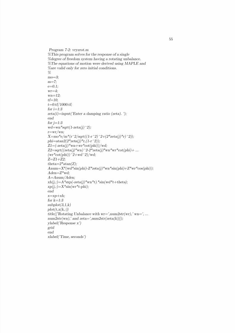
Program 7-2: vryzrot.m%This program solves for the response of a single
%degree of freedom system having a rotating unbalance.%The equations of motion were derived using MAPLE and %are valid only for zero initial conditions.%mo=3;m=7;e=0.1;wr=4;wn=12;tf=10;t=0:tf/1000:tf;for i=1:3 zeta(i)=input(’Enter a damping ratio (zeta). ’);end for j=1:3 wd=wn*sqrt(1-zeta(j)^2);r=wr/wn;X=mo*e/m*(r̂ 2/sqrt((1-r^2)^2+(2*zeta(j)*r)^2));
phi=atan2(2*zeta(j)*r,(1-r^2));Z1=(-zeta(j)*wn+wr*cot(phi))/wd;Z2=sqrt((zeta(j)*wn)^2-2*zeta(j)*wn*wr*cot(phi)+ ...(wr*cot(phi))^2+wd^2)/wd;Z=Z1+Z2;theta=2*atan(Z);Anum=X*(wd*sin(phi)-Z*zeta(j)*wn*sin(phi)+Z*wr*cos(phi));
Aden=Z*wd;A=Anum/Aden;xh(j,:)=A*exp(-zeta(j)*wn*t).*sin(wd*t+theta);xp(j,:)=X*sin(wr*t-phi);end x=xp+xh;for k=1:3 subplot(3,1,k)
plot(t,x(k,:))title([’Rotating Unbalance with wr=’,num2str(wr),’ wn=’, ...num2str(wn),’ and zeta=’,num2str(zeta(k))]);
ylabel(’Response x’)grid
end xlabel(’Time, seconds’)

8/20/2019 Vibrations Using Matlab
http://slidepdf.com/reader/full/vibrations-using-matlab 61/170
56CHAPTER 8 SDOF SYSTEMS WITH A ROTATING UNBALANCE
Program 7-3: vrymrot.m%This program solves for the response of a single
%degree of freedom system having a rotating unbalance.%The equations of motion were derived using MAPLE and %are valid only for zero initial conditions.%mo=3;zeta=0.05;e=0.1;wr=4;wn=12;tf=10;t=0:tf/1000:tf;for i=1:3 m(i)=input(’Enter a system mass. ’);end for j=1:3 wd=wn*sqrt(1-zeta^2);r=wr/wn;X=mo*e/m(j)*(r^2/sqrt((1-r 2̂)^2+(2*zeta*r)^2));
phi=atan2(2*zeta*r,(1-r^2));Z1=(-zeta*wn+wr*cot(phi))/wd;Z2=sqrt((zeta*wn)^2-2*zeta*wn*wr*cot(phi)+ ...(wr*cot(phi))^2+wd^2)/wd;Z=Z1+Z2;theta=2*atan(Z);Anum=X*(wd*sin(phi)-Z*zeta*wn*sin(phi)+Z*wr*cos(phi));
Aden=Z*wd;A=Anum/Aden;xh(j,:)=A*exp(-zeta*wn*t).*sin(wd*t+theta);xp(j,:)=X*sin(wr*t-phi);end x=xp+xh;for k=1:3 subplot(3,1,k)
plot(t,x(k,:))title([’Rotating Unbalance with wr=’,num2str(wr),’, wn=’, ...num2str(wn),’, mass=’,num2str(m(k)),’, and rotating mass=’, ...num2str(mo)]);grid
end xlabel(’Time, seconds’)

8/20/2019 Vibrations Using Matlab
http://slidepdf.com/reader/full/vibrations-using-matlab 62/170
57
0 1 2 3 4 5 6 7 8 9 10-0.2
0
0.2
Rotating Unbalance with wr=4 wn=2 and zeta=0.05
0 1 2 3 4 5 6 7 8 9 10-0.05
0
0.05
Rotating Unbalance with wr=4 wn=6 and zeta=0.05
0 1 2 3 4 5 6 7 8 9 10-0.01
0
0.01
Time, seconds
Rotating Unbalance with wr=4 wn=12 and zeta=0.05
Figure 8.2: Response of systems with di¤erent natural frequencies to a rotatingunbalance.

8/20/2019 Vibrations Using Matlab
http://slidepdf.com/reader/full/vibrations-using-matlab 63/170
58CHAPTER 8 SDOF SYSTEMS WITH A ROTATING UNBALANCE
0 1 2 3 4 5 6 7 8 9-0.01
0
0.01
R e s p o n s e x
Rotating Unbalance with wr=4 wn=12 and zeta=0.05
0 1 2 3 4 5 6 7 8 9-0.01
0
0.01
R e s p o n s e x
Rotating Unbalance with wr=4 wn=12 and zeta=0.1
0 1 2 3 4 5 6 7 8 9-0.01
0
0.01
Time, seconds
R e s p o n s e x
Rotating Unbalance with wr=4 wn=12 and zeta=0.3
Figure 8.3: Response with varied damping ratios.
8/20/2019 Vibrations Using Matlab
http://slidepdf.com/reader/full/vibrations-using-matlab 64/170
59
0 1 2 3 4 5 6 7 8 9 10-0.05
0
0.05
Rotating Unbalance with wr=4, wn=12, mass=1, and rotating mass=3
0 1 2 3 4 5 6 7 8 9 10-0.02
0
0.02
Rotating Unbalance with wr=4, wn=12, mass=3, and rotating mass=3
0 1 2 3 4 5 6 7 8 9 10-0.01
0
0.01
Time, seconds
Rotating Unbalance with wr=4, wn=12, mass=6, and rotating mass=3
Figure 8.4: E¤ects of varying system mass.

8/20/2019 Vibrations Using Matlab
http://slidepdf.com/reader/full/vibrations-using-matlab 65/170

8/20/2019 Vibrations Using Matlab
http://slidepdf.com/reader/full/vibrations-using-matlab 66/170
Chapter 9
Impulse Response of SDOF
Systems
In the previous few examples, we have discussed the response of single degreeof freedom systems to di¤erent forms of sinusoidal inputs. In the followingexamples, we will examine the e¤ects of non-sinusoidal inputs on single degreeof freedom systems. The simplest of these is the impulse response.
An impulse is a force which is applied over a very short time when comparedto the period of vibration. The period over which the impulse is applied isassumed to be 2: If the impulse is centered about time t, then it is appliedfrom t to t + : If the force has a total value of F o; then the average value isF o=2: So, for all time except the interval around t, the value of the impulse is0; within the interval, it is F o=2:
Using the de…nition of impulse as force multiplied by time, and noting thatimpulse is the change in momentum, we see that:
(F o=2) 2 = mvo; (9.1)
where vo is the initial velocity of the system. This is because the velocity of thesystem before the impulse is zero, and it is vo after the impulse. So, this problemreduces to a single degree of freedom free vibration with zero initial displacementand initial velocity equal to F o=m: Recall that for a damped oscillator, theresponse is of the form:
x(t) = Ae!t sin(!dt + ): (9.2)
Since
A =p
(vo + !xo)2 + (xo!d)2=!d, = tan1 (xo!d= (vo + !xo)) ;
61
8/20/2019 Vibrations Using Matlab
http://slidepdf.com/reader/full/vibrations-using-matlab 67/170
62 CHAPTER 9 IMPULSE RESPONSE OF SDOF SYSTEMS
we note that, for xo = 0, A = vo=!d, and = 0. Thus, Equation 9.2 becomes
x(t) = F o!d
e!t sin(!dt): (9.3)
This response, as noted above, is simply a single degree of freedom oscillatorsubject to an initial velocity. The behavior with changing F o is similar tochanging vo in a single degree of freedom oscillator. For that reason, a programand plots for this situation are not included; they would be the same as thosein Example 2. Included in this example is a program which simulates the Diracdelta function (an impulse with F o = 1), for an impulse around a given time andwith a given total time interval. The program simply takes the entire intervaland sets the function equal to zero for all times other than the one speci…ed,and equal to one for the speci…ed time.
Program 8-2 gives an example of how this delta function can be used insideof another program, by plotting the function over a speci…ed time interval. Thisprogram makes use of subfunctions as well. This is more handy for single-usefunctions, such as several of the unwieldy constants we derived for some of ourearlier examples. A subfunction is called just like any other MATLAB function.The subfunction is written after the main code, and is internal to the code.The variables used inside the subfunction stay in the subfunction; they are notintroduced to the MATLAB workspace. Thus, if we tried to use the variable“int” in the main code of Program 8-2, we would generate an error. One moreitem of note is the “ndelta” in the ylabel function call. That is a LaTEXtag, which is usable inside of a MATLAB string. Notice the results when theprogram is run; the y-axis reads “ (td) ; " substituting the value entered for td:
Superscripts, subscripts, Greek characters, and other useful e¤ects are availablein this manner; “help latex” at the MATLAB prompt can give you a start onusing these.
8/20/2019 Vibrations Using Matlab
http://slidepdf.com/reader/full/vibrations-using-matlab 68/170
63
Program 8-1: delta.m
function delta=delta(td,tf)
%This function simulates the delta function.
%The user must input the time at which the
%nonzero value is desired, td, and the ending time, tf.
%
int=tf*td;
%The variable int ensures that a value in the time vector
%will match the desired time. The strategy is to subdivide
%the interval into at least 500 steps (this ensures the
%interval over which the function is nonzero is small).
%
while int<500
int=int*10;end
t=0:tf/int:tf;
for i=1:int
if t(i)==td
delta(i)=1;
else
delta(i)=0;
end
end
8/20/2019 Vibrations Using Matlab
http://slidepdf.com/reader/full/vibrations-using-matlab 69/170
64 CHAPTER 9 IMPULSE RESPONSE OF SDOF SYSTEMS
%Program 8-2: subdemo.mfunction [t,y]=subdemo(td,tf)
%% A simple routine to demonstrate use of subfunctions,% making use of the delta function as an example.% Inputs are the time of the delta function, td,% and the overall timespan, tf.% Note that subfunctions cannot be used % inside of script m-…les. If we were to % write Program 8-2 as a script (like most of % our m-…les to this point), the delta function% would have to be external.%
y=subdelta(td,tf);% Calling the subfunction version “subdelta”% guarantees we’ll be calling the subfunction,% not the function from Program 8-1.% Now that we have the value of the delta function,% we need to create a time vector that goes from% zero to tf, and has the same number of points % as the vector y (else we will get a plotting % error). For this, we use the “max” and % “size” commands.len=max(size(y));% “size” returns the vector [nrows ncols], corresponding % to the number of rows and columns in y. Taking the % maximum will return the longer dimension, and is a
% shortcut usable for both row and column vectors.t=linspace(0,tf,len);% “linspace” is much more natural a command for this % instance than the colon operator. This will generate % a vector with len equally-spaced elements between% 0 and tf.
plot(t,y)title(’Delta Function Sample’);
ylabel([’ ndelta(’,num2str(td),’)’]);xlabel(’Time, seconds’);grid function delta=subdelta(td,tf)% This function is Program 8-1.
% Note that a subfunction is included % with a “function” call, just like an% external function.int=tf*td;while int<500 int=int*10;

8/20/2019 Vibrations Using Matlab
http://slidepdf.com/reader/full/vibrations-using-matlab 70/170
65
end t=0:tf/int:tf;
for i=1:intif t(i)==td delta(i)=1;else delta(i)=0;end
end

8/20/2019 Vibrations Using Matlab
http://slidepdf.com/reader/full/vibrations-using-matlab 71/170

8/20/2019 Vibrations Using Matlab
http://slidepdf.com/reader/full/vibrations-using-matlab 72/170
Chapter 10
Step Response of a SDOF
System
In this example, the force is assumed to be applied instantaneously, but it willbe sustained out to in…nity. This is essentially an on-function . If a force of thissort is plotted versus time, the force looks like a step up. So then, the behaviorof the system under this type of load is considered the step response of the singledegree of freedom system. We assume the system is underdamped and will havezero initial conditions. We already know the equation of motion,
::x + 2!n
:x + !2
nx = F (t)=m; (10.1)
where
F (t) =
8<: 0 if 0 < t < to
F o if t to: (10.2)
In order to solve the di¤erential equation, we will use the convolution integral
x(t) =
Z t0
F ( )g(t )d : (10.3)
Recall that the convolution integral is derived by treating the force as an in-…nite series of impulse forces. The …rst fundamental theorem of calculus then
allows the in…nite series to be treated as the integral given above. The impulseresponse, just discussed, given by
x(t) = F om!d
e!nt sin !dt = F og(t); (10.4)
67

8/20/2019 Vibrations Using Matlab
http://slidepdf.com/reader/full/vibrations-using-matlab 73/170
68 CHAPTER 10 STEP RESPONSE OF A SDOF SYSTEM
where we know that
g(t) = 1
m!de!t sin !dt: (10.5)
Therefore,
x(t) = 1
m!de!nt
Z t0
F ( )e!n sin !d(t )d : (10.6)
Now, since we have a general expression for x(t), we can substitute our F (t)into Equation 10.6 to give:
x(t) = 1
m!de!nt
Z to0
(0)e!n sin !d(t )d +
Z tto
F oe!n sin !d(t )d
:
(10.7)
Note that the …rst term inside the braces is zero. For that reason, for t < to,the response of the system is zero. To …nd the response for all other times, wemust evaluate the second integral (by parts):
x(t) = F o
k
(1 1
p 1 2e!n(tto) cos[!d(t to) ]
); t to; (10.8)
where = tan1 p 12
: It is important to remember that this equation is
only valid for the time after the force is applied; the response is zero beforeapplication of the force.
Figure 10.1 shows the variation of the response with the force magnitude. Asmight be expected, the only di¤erence that results from changing the magnitudeof the external force is that the magnitude of the response changes. That is,the magnitude of the response is directly proportional to the magnitude of theexternal force. The magnitude of the external force also causes a second di¤er-ence: note that when the oscillatory motion begins, it is not centered aroundzero. Instead, the mass oscillates around a displacement greater than zero. Thevalue of this center point is also dependent on the magnitude of the external
force (from the term 1 in the Equation 10.8).In Figure 10.2, we vary the natural frequency. This causes two changes in
the response. First, the rate of exponential decrease in the response (the e¤ectof damping) is increased; that is, the response stabilizes more quickly. Second,the oscillation frequency decreases, since the natural frequency also dictates thedamped frequency.
8/20/2019 Vibrations Using Matlab
http://slidepdf.com/reader/full/vibrations-using-matlab 74/170
69
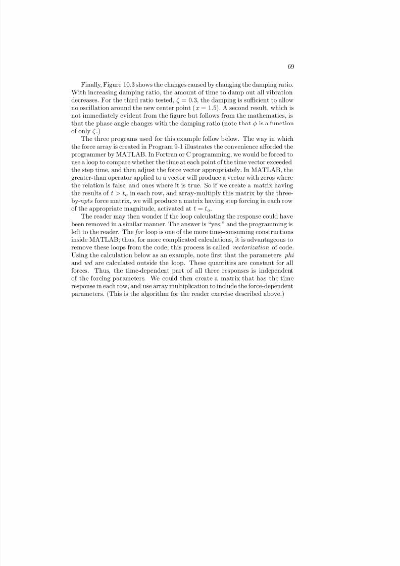
Finally, Figure 10.3 shows the changes caused by changing the damping ratio.With increasing damping ratio, the amount of time to damp out all vibration
decreases. For the third ratio tested, = 0:3, the damping is su¢cient to allowno oscillation around the new center point (x = 1:5). A second result, which isnot immediately evident from the …gure but follows from the mathematics, isthat the phase angle changes with the damping ratio (note that is a functionof only .)
The three programs used for this example follow below. The way in whichthe force array is created in Program 9-1 illustrates the convenience a¤orded theprogrammer by MATLAB. In Fortran or C programming, we would be forced touse a loop to compare whether the time at each point of the time vector exceededthe step time, and then adjust the force vector appropriately. In MATLAB, thegreater-than operator applied to a vector will produce a vector with zeros wherethe relation is false, and ones where it is true. So if we create a matrix havingthe results of t > to in each row, and array-multiply this matrix by the three-by-npts force matrix, we will produce a matrix having step forcing in each rowof the appropriate magnitude, activated at t = to:
The reader may then wonder if the loop calculating the response could havebeen removed in a similar manner. The answer is “yes,” and the programming isleft to the reader. The for loop is one of the more time-consuming constructionsinside MATLAB; thus, for more complicated calculations, it is advantageous toremove these loops from the code; this process is called vectorization of code.Using the calculation below as an example, note …rst that the parameters phiand wd are calculated outside the loop. These quantities are constant for allforces. Thus, the time-dependent part of all three responses is independentof the forcing parameters. We could then create a matrix that has the timeresponse in each row, and use array multiplication to include the force-dependent
parameters. (This is the algorithm for the reader exercise described above.)

8/20/2019 Vibrations Using Matlab
http://slidepdf.com/reader/full/vibrations-using-matlab 75/170
70 CHAPTER 10 STEP RESPONSE OF A SDOF SYSTEM
Program 9-1: stepfm.m%This program calculates the step response
%of a single degree of freedom system. This %version tests three di¤erent force magnitudes.%The program assumes a system mass of 1.%zeta=0.05;tf=10;npts=1000;t=linspace(0,tf,npts);to=2;wn=12;k=(wn)^2;for i=1:3
Fm(i,1)=input(’Enter a force magnitude. ’); % Forcing Fm to be a column vector.
end Fint=Fm*ones(1,npts); % Fint is thus 3-by-npts.%% Now, we perform the logical operation t>to,% and make a 3-by-npts matrix of the result.%qtest=t>to;fmult=[qtest;qtest;qtest]; % Three rows of qtest.Fo=Fint.*fmult; % The force matrix.wd=wn*sqrt(1-zeta^2);
phi=atan2(zeta,sqrt(1-zeta^2));
for n=1:3 A=Fo(n,:)/k;B=Fo(n,:)/(k*sqrt(1-zeta^2));x(n,:)=A-B.*exp(-zeta*wn*t).*cos(wd*t-phi);
end for l=1:3
subplot(3,1,l) plot(t,x(l,:))title([’Response for wn=’,num2str(wn),’, Fmax=’, ...num2str(Fm(l)),’, and time=’, num2str(to)]);
ylabel(’Response x’)grid
end
xlabel(’Time, seconds’)

8/20/2019 Vibrations Using Matlab
http://slidepdf.com/reader/full/vibrations-using-matlab 76/170
71
Program 9-2: stepwn.m%This program calculates the step response
%of a single degree of freedom system. This %version tests three di¤erent natural frequencies.%The program assumes a system mass of 1.%Fm=5;npts=1000;zeta=0.05;tf=10;t=linspace(0,tf,npts);to=2;qtest=t>to; % Only one force vector here, so we can do this here.Fo=Fm*qtest; % Scalar Fm * 1-by-npts vector.for i=1:3
wn(i)=input(’Enter a natural frequency. ’);k(i)=wn(i)^2;
end %% This could also be vectorized.%for n=1:3
wd=wn(n)*sqrt(1-zeta^2);A=Fo/k(n);B=Fo/(k(n)*sqrt(1-zeta^2));
phi=atan2(zeta,sqrt(1-zeta^2));x(n,:)=A-B.*exp(-zeta*wn(n)*t).*cos(wd*t-phi);
end for l=1:3 subplot(3,1,l)
plot(t,x(l,:))title([’Response for wn=’,num2str(wn(l)),’, Fmax=’, ...
num2str(Fm),’, and time=’, num2str(to)]); ylabel(’Response x’)grid
end xlabel(’Time, seconds’)

8/20/2019 Vibrations Using Matlab
http://slidepdf.com/reader/full/vibrations-using-matlab 77/170
72 CHAPTER 10 STEP RESPONSE OF A SDOF SYSTEM
Program 9-3: stepzeta.m%This program calculates the step response
%of a single degree of freedom system. This %version tests three di¤erent natural frequencies.%The program assumes a system mass of 1.%npts=1000;Fm=5;tf=10;t=linspace(0,tf,npts);to=2;qtest=t>to;Fo=Fm*qtest;wn=12;k=(wn)^2;for i=1:3
zeta(i)=input(’Enter a damping ratio (zeta). ’);end %% This could also be vectorized.%for n=1:3
wd=wn*sqrt(1-zeta(n)^2);A=Fo/k;B=Fo/(k*sqrt(1-zeta(n)^2));
phi=atan2(zeta(n),sqrt(1-zeta(n)̂ 2));x(n,:)=A-B.*exp(-zeta(n)*wn*t).*cos(wd*t-phi);
end for l=1:3 subplot(3,1,l)
plot(t,x(l,:))title([’Response for wn=’,num2str(wn),’, zeta=’, ...
num2str(zeta(l)),’, and time=’, num2str(to)]); ylabel(’Response x’)grid
end xlabel(’Time, seconds’)

8/20/2019 Vibrations Using Matlab
http://slidepdf.com/reader/full/vibrations-using-matlab 78/170
73
0 1 2 3 4 5 6 7 8 9 100
0.01
0.02
0.03
R e s p o n s e x
Response for wn=12, Fmax=3, and time=2
0 1 2 3 4 5 6 7 8 9 100
0.05
0.1
R e s p o n s e
x
Response for wn=12, Fmax=7, and time=2
0 1 2 3 4 5 6 7 8 9 100
0.05
0.1
Time, seconds
R e s p o n s e
x
Response for wn=12, Fmax=11, and time=2
Figure 10.1: Step response of a single degree of freedom system to di¤erent stepmagnitudes.

8/20/2019 Vibrations Using Matlab
http://slidepdf.com/reader/full/vibrations-using-matlab 79/170
74 CHAPTER 10 STEP RESPONSE OF A SDOF SYSTEM
0 1 2 3 4 5 6 7 8 90
0.5
R e s p o n s e x
Response for wn=4, Fmax=5, and time=2
0 1 2 3 4 5 6 7 8 90
0.1
R e s p o n s e
x
Response for wn=7, Fmax=5, and time=2
0 1 2 3 4 5 6 7 8 90
0.02
0.04
0.06
Time, seconds
R e s p o n s e
x
Response for wn=12, Fmax=5, and time=2
Figure 10.2: Step response of single degree of freedom systems having di¤erentnatural frequencies.
8/20/2019 Vibrations Using Matlab
http://slidepdf.com/reader/full/vibrations-using-matlab 80/170
75
0 1 2 3 4 5 6 7 8 9 100
0.02
0.04
0.06
R e s p o n s e x
Response for wn=12, zeta=0.05, and time=2
0 1 2 3 4 5 6 7 8 9 100
0.02
0.04
R e s p o n s e
x
Response for wn=12, zeta=0.1, and time=2
0 1 2 3 4 5 6 7 8 9 100
0.02
0.04
Time, seconds
R e s p o n s e
x
Response for wn=12, zeta=0.3, and time=2
Figure 10.3: Step response of a single degree of freedom system to di¤erentlevels of damping.

8/20/2019 Vibrations Using Matlab
http://slidepdf.com/reader/full/vibrations-using-matlab 81/170
8/20/2019 Vibrations Using Matlab
http://slidepdf.com/reader/full/vibrations-using-matlab 82/170
Chapter 11
Response of SDOF Systems
to Square Pulse Inputs
A square pulse is a single pulse of constant magnitude and …nite duration. Toanalyze the response of systems to a square wave input, we will treat the squarewave as the sum of two equal and opposite step inputs applied at di¤erent times.The time interval between application of the step inputs is the duration of thesquare wave.
Let us assume that the magnitude of the square wave is F o, and its durationis t1 seconds. To simulate the wave using step inputs, we begin with a stepinput of magnitude F o from time t = 0; and add to it at time t1 a step input of magnitude F o: By superposition, the total response is the sum of the responseof the system to each step input.
Recall that the response of a single degree of freedom system to a step inputof magnitude F m applied at time to is:
x(t) = F m
k
(1 1p
1 2e!n(tto) cos[!d (t to) ]
); t to; (11.1)
where = arctan =p
1 2: If we now consider the two step inputs separately,denoting the response of the system to the input at time t = 0 as x1(t) and theresponse to the input at time t = t1 as x2(t); we …nd that:
x1(t) = F o
k
(1 1p
1 2e!t cos[!dt ]
); t 0 (11.2)
and
77

8/20/2019 Vibrations Using Matlab
http://slidepdf.com/reader/full/vibrations-using-matlab 83/170
78CHAPTER 11 RESPONSE OF SDOF SYSTEMS TO SQUARE PULSE INPUTS
x2(t) = F ok
(1 1p
1 2e!(tt1) cos[!d (t t1) ]
); t t1: (11.3)
The total response is then:
x(t) = F o
k
(1 1p
1 2e!nt cos[!dt ]
); 0 t < t1; (11.4)
x(t) = F oe!nt
kp
1
2 e!nt1 cos[!d (t t1) ] cos(!dt ) ; t t1: (11.5)
Notice how, for the time interval after t1, the response no longer includes a\1 " term; the addition of the two responses has removed this term entirely.Again recalling a previous example, the \1 " term caused the oscillation to beabout a new equilibrium (i.e., x = F o=k). Now, since the term has disappeared,the oscillation is centered around zero.
The movement of the center point of the oscillation is best shown in Figure11.1, which tests three di¤erent values of F o: The oscillation begins about acenter point at x = F o=k: When the square wave ends, or, when the equaland opposite step is added, the center point returns to zero. Assume, for amoment, that the magnitude of the second step is not equal to that of the…rst; call it F 1: In this case, the center point of the oscillation after adding
the second step input would be at x = (F o F 1) =k: To prove this to yourself,perform the superposition used to obtain Equation 11.5, above (remember thatF 1 is negative!). A constant term will remain, and this term will be equal to(F o F 1) =k: Another result which is evident from Figure 10.1 is that the changein F o causes the magnitude of the oscillations to increase, as would be expectedfrom Equation 11.5.
Figure 11.2 shows the e¤ects of changing the natural frequency. Notice thata transition point occurs when the second step input is added. The sudden shiftin vibration characteristics is expected, since we have a piecewise expression forx(t): But note that while the transition becomes more abrupt as the naturalfrequency increases, it is never discontinuous. Since the motion of the massremains continuous, we can infer that the approach is correct; if we had obtaineda discontinuity in the motion, we would know the expression is incorrect. This
is because a discontinuous expression would imply that the mass moved fromone point to another nonadjacent point without passing through the points inbetween, a physically impossible situation.
Finally, Figure 11.3 demonstrates the response behavior for three di¤erentdamping ratios. Again, notice how the high damping ratio ( = 0:3) causes allof the vibration to be damped out quickly, so that the mass is practically at rest

8/20/2019 Vibrations Using Matlab
http://slidepdf.com/reader/full/vibrations-using-matlab 84/170
79
when the second step input is applied. Again, we see that the transient perioddecreases with increasing damping ratio.
The MATLAB code to produce these …gures demonstrates the vectorizationdiscussed in the previous example. Note how the logical operation t < to is usedto create a matrix of zeros and ones, where the ones correspond to times beforeto: Then the MATLAB “not” operator (the tilde, ~) is used to arrive at timesafter to: The reader is encouraged to rewrite the vectorized calculation as a loop(in any of the three codes) and see for himself the di¤erence in time expenditureas the number of points is increased by a few orders of magnitude. While thereare no fewer actual calculations performed in the vectorized code, the di¤erenceis that MATLAB’s vector/matrix calculations are highly optimized, and so thecode is faster when handling one matrix calculation instead of many scalarcalculations.
One more di¤erence between these codes and the previous is that we’veinserted another use of the colon operator. As explained in Program 10-1, thestatement a = b(:); has a particular meaning in MATLAB. For a vector b;MATLAB will return a column vector a that is equal to a column vector b orthe transpose of a row vector b: That is, if we wish to be certain whether a vectorwe are working with is a column vector, then we can use the colon operator inthis manner to force it to be so; the output of a = b(:) is a column vector forany vector b:
Another interesting consequence of this use of the colon operator is the resultfor a matrix b: The colon operator would return a column vector a consisting of the rows of b stacked on top of each other. The reader is encouraged to try this,and see the results. Additionally, what would we do if we wanted to force a to bea row vector? Finally, what if we wished to make these script instead functions,taking the number of points in the time vector as inputs? How would we modify
the code then? The advantage would be that all the variables from the functionwould not become part of our workspace. Often, this is a disadvantage from adebugging perspective, but is very nice to have in working code.
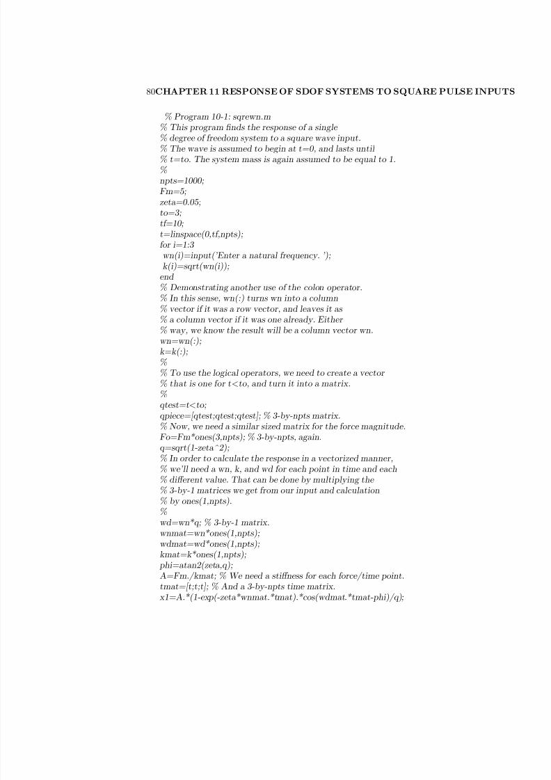
8/20/2019 Vibrations Using Matlab
http://slidepdf.com/reader/full/vibrations-using-matlab 85/170
80CHAPTER 11 RESPONSE OF SDOF SYSTEMS TO SQUARE PULSE INPUTS
% Program 10-1: sqrewn.m% This program …nds the response of a single
% degree of freedom system to a square wave input.% The wave is assumed to begin at t=0, and lasts until % t=to. The system mass is again assumed to be equal to 1.%npts=1000;Fm=5;zeta=0.05;to=3;tf=10;t=linspace(0,tf,npts);for i=1:3 wn(i)=input(’Enter a natural frequency. ’);k(i)=sqrt(wn(i));
end % Demonstrating another use of the colon operator.% In this sense, wn(:) turns wn into a column% vector if it was a row vector, and leaves it as % a column vector if it was one already. Either % way, we know the result will be a column vector wn.wn=wn(:);k=k(:);%% To use the logical operators, we need to create a vector % that is one for t<to, and turn it into a matrix.%
qtest=t<to;qpiece=[qtest;qtest;qtest]; % 3-by-npts matrix.% Now, we need a similar sized matrix for the force magnitude.Fo=Fm*ones(3,npts); % 3-by-npts, again.q=sqrt(1-zeta^2);% In order to calculate the response in a vectorized manner,% we’ll need a wn, k, and wd for each point in time and each% di¤erent value. That can be done by multiplying the % 3-by-1 matrices we get from our input and calculation% by ones(1,npts).%wd=wn*q; % 3-by-1 matrix.wnmat=wn*ones(1,npts);
wdmat=wd*ones(1,npts);kmat=k*ones(1,npts);
phi=atan2(zeta,q);A=Fm./kmat; % We need a sti¤ness for each force/time point.tmat=[t;t;t]; % And a 3-by-npts time matrix.x1=A.*(1-exp(-zeta*wnmat.*tmat).*cos(wdmat.*tmat-phi)/q);
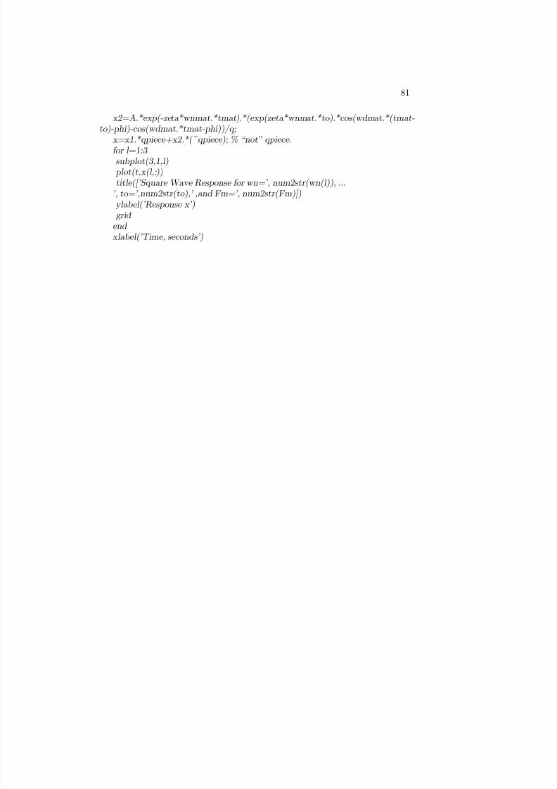
8/20/2019 Vibrations Using Matlab
http://slidepdf.com/reader/full/vibrations-using-matlab 86/170
81
x2=A.*exp(-zeta*wnmat.*tmat).*(exp(zeta*wnmat.*to).*cos(wdmat.*(tmat-to)-phi)-cos(wdmat.*tmat-phi))/q;
x=x1.*qpiece+x2.*(~qpiece); % “not” qpiece.for l=1:3 subplot(3,1,l)
plot(t,x(l,:))title([’Square Wave Response for wn=’, num2str(wn(l)), ...
’, to=’,num2str(to),’ ,and Fm=’, num2str(Fm)]) ylabel(’Response x’)grid
end xlabel(’Time, seconds’)

8/20/2019 Vibrations Using Matlab
http://slidepdf.com/reader/full/vibrations-using-matlab 87/170
82CHAPTER 11 RESPONSE OF SDOF SYSTEMS TO SQUARE PULSE INPUTS
%Program 10-2: sqrefm.m%This program …nds the response of a single
%degree of freedom system to a square wave input.%The wave is assumed to begin at t=0, and lasts until %t=to. The system mass is again assumed to be equal to 1.%npts=1000;wn=11;k=(wn)^2;zeta=0.05;to=3;tf=10;t=linspace(0,tf,npts);for i=1:3 Fm(i)=input(’Enter a force magnitude. ’);
end Fm=Fm(:); % See above.% As with the step response example earlier,% we can use MATLAB’s logical operators to % create a piecewise function without resorting % to a loop. This can be done with the % statement: qtest=(t>t1)-(t>t2), when% the square wave begins at t=t1 and ends at% t=t2. For the case of t1=0, a simpler % statement is valid:qtest=(t<to);Fo=Fm*ones(1,npts); % Since solution is piecewise, we need Fm throughout.
% This code demonstrates vectorization of this % piecewise expression. We’ll be making use of % the qtest vector above to tell the code when% to activate each solution.%qpiece=[qtest;qtest;qtest]; % One row for each Fm value.q=sqrt(1-zeta^2);wd=wn*q;
phi=atan2(zeta,q);A=Fo/k; % 3-by-npts matrix.tmat=[t;t;t]; % Again, 3-by-npts.x1=A.*(1-exp(-zeta*wn*tmat).*cos(wd*tmat-phi)/q); % Solution for t<to.x2=A.*exp(-zeta*wn*tmat).*(exp(zeta*wn*to).*cos(wd*(tmat-to)-phi)-cos(wd*tmat-
phi))/q;x=x1.*qpiece+x2.*(~qpiece); % ~is the “not” operator.for l=1:3 subplot(3,1,l)
plot(t,x(l,:))title([’Square Wave Response for wn=’, num2str(wn), ...

8/20/2019 Vibrations Using Matlab
http://slidepdf.com/reader/full/vibrations-using-matlab 88/170
83
’, to=’,num2str(to),’ ,and Fm=’, num2str(Fm(l))])
ylabel(’Response x’)
grid
end
xlabel(’Time, seconds’)
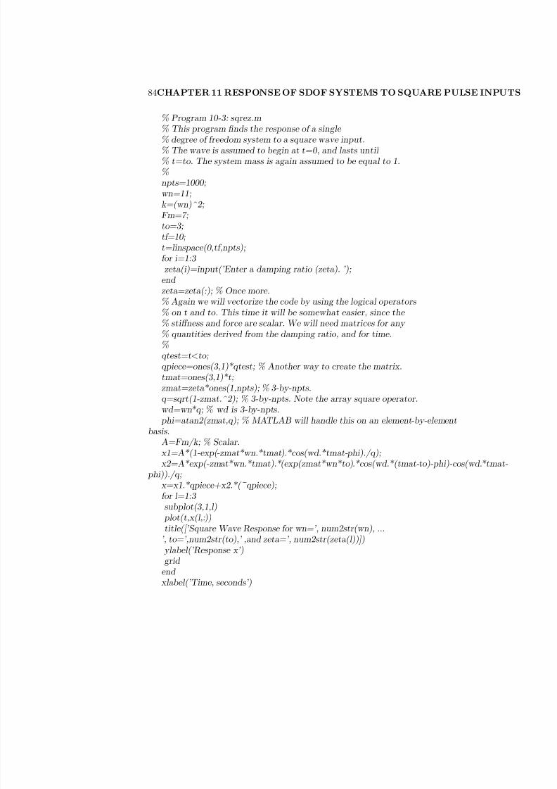
8/20/2019 Vibrations Using Matlab
http://slidepdf.com/reader/full/vibrations-using-matlab 89/170
84CHAPTER 11 RESPONSE OF SDOF SYSTEMS TO SQUARE PULSE INPUTS
% Program 10-3: sqrez.m% This program …nds the response of a single
% degree of freedom system to a square wave input.% The wave is assumed to begin at t=0, and lasts until % t=to. The system mass is again assumed to be equal to 1.%npts=1000;wn=11;k=(wn)^2;Fm=7;to=3;tf=10;t=linspace(0,tf,npts);for i=1:3 zeta(i)=input(’Enter a damping ratio (zeta). ’);
end zeta=zeta(:); % Once more.% Again we will vectorize the code by using the logical operators % on t and to. This time it will be somewhat easier, since the % sti¤ness and force are scalar. We will need matrices for any % quantities derived from the damping ratio, and for time.%qtest=t<to;qpiece=ones(3,1)*qtest; % Another way to create the matrix.tmat=ones(3,1)*t;zmat=zeta*ones(1,npts); % 3-by-npts.q=sqrt(1-zmat.^2); % 3-by-npts. Note the array square operator.
wd=wn*q; % wd is 3-by-npts. phi=atan2(zmat,q); % MATLAB will handle this on an element-by-elementbasis.
A=Fm/k; % Scalar.x1=A*(1-exp(-zmat*wn.*tmat).*cos(wd.*tmat-phi)./q);x2=A*exp(-zmat*wn.*tmat).*(exp(zmat*wn*to).*cos(wd.*(tmat-to)-phi)-cos(wd.*tmat-
phi))./q;x=x1.*qpiece+x2.*(~qpiece);for l=1:3 subplot(3,1,l)
plot(t,x(l,:))title([’Square Wave Response for wn=’, num2str(wn), ...
’, to=’,num2str(to),’ ,and zeta=’, num2str(zeta(l))])
ylabel(’Response x’)grid
end xlabel(’Time, seconds’)

8/20/2019 Vibrations Using Matlab
http://slidepdf.com/reader/full/vibrations-using-matlab 90/170
85
0 1 2 3 4 5 6 7 8 9 10-0.05
0
0.05
R e s p o n s e
x
Square Wave Response for wn=11, to=3 ,and Fm=3
0 1 2 3 4 5 6 7 8 9 10
0
0.2
R e s p o n s e
x
Square Wave Response for wn=11, to=3 ,and Fm=7
0 1 2 3 4 5 6 7 8 9 10
0
0.2
Time, seconds
R e s p o n s e
x
Square Wave Response for wn=11, to=3 ,and Fm=11
Figure 11.1: Plot of responses for three di¤erent force magnitudes.

8/20/2019 Vibrations Using Matlab
http://slidepdf.com/reader/full/vibrations-using-matlab 91/170
86CHAPTER 11 RESPONSE OF SDOF SYSTEMS TO SQUARE PULSE INPUTS
0 1 2 3 4 5 6 7 8 9-5
0
5
R e s p o n s e
x
Square Wave Response for wn=4, to=3 ,and Fm=5
0 1 2 3 4 5 6 7 8 9-2
0
2
4
R e s p o n s e
x
Square Wave Response for wn=8, to=3 ,and Fm=5
0 1 2 3 4 5 6 7 8 9-2
0
2
4
Time, seconds
R e s p o n s e
x
Square Wave Response for wn=12, to=3 ,and Fm=5
Figure 11.2: Square wave response variation with di¤erent natural frequencies.
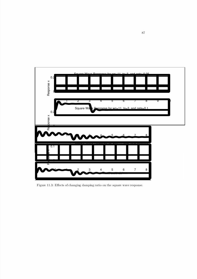
8/20/2019 Vibrations Using Matlab
http://slidepdf.com/reader/full/vibrations-using-matlab 92/170
87
0 1 2 3 4 5 6 7 8 9 10
0
0.2
R e s p o n s e
x
Square Wave Response for wn=11, to=3 ,and zeta=0.05
0 1 2 3 4 5 6 7 8 9 10
0
0.2
R e s p o n s e
x
Square Wave Response for wn=11, to=3 ,and zeta=0.1
0 1 2 3 4 5 6 7 8 9 10
0
0.1
Time, seconds
R e s p o n s e
x
Square Wave Response for wn=11, to=3 ,and zeta=0.3
Figure 11.3: E¤ects of changing damping ratio on the square wave response.

8/20/2019 Vibrations Using Matlab
http://slidepdf.com/reader/full/vibrations-using-matlab 93/170

8/20/2019 Vibrations Using Matlab
http://slidepdf.com/reader/full/vibrations-using-matlab 94/170
Chapter 12
Response of SDOF System
to Ramp Input
Another common form of input encountered in real applications is the rampinput. To examine the response of a single degree of freedom system to this sortof input, we must again apply the convolution integral. Assuming that the loadis increased uniformly at a rate of f o per second and reaches its maximum attime td; then the expression for the external force is:
F (t) =
8<:
f ot for 0 t < td;
f otd for t
td:
(12.1)
Substituting the expression for F (t) into the convolution integral yields:
x(t) =
8<:
f om!d
e!ntR t0
e!n sin !d(t )d for 0 t < td;
f om!d
e!nthR td
0 e!n sin !d(t )d + td
R ttd
e!n sin !d(t )d i
for t td:
(12.2)
This expression is best evaluated using MAPLE or a table of integrals.
x(t) = f om!d
e!nt
1 2!2
n + !2d
2
!de!nt
t 2!2n + t!2
d 2!n
+ 2!n!d cos(!dt)
+
2!2n !2
d
sin(!dt)
; 0 t < td;
89

8/20/2019 Vibrations Using Matlab
http://slidepdf.com/reader/full/vibrations-using-matlab 95/170
90CHAPTER 12 RESPONSE OF SDOF SYSTEM TO RAMP INPUT
x(t) = f om!d
e!nt
1 2!2
n + !2d
2!de!nt
t 2!2n + t!2
d 2!n
+ 2!n!d cos(!dt)
+
2!2n !2
d
sin(!dt)
+
f otdk f otd
kp
1 2e!n(ttd) cos(!d(ttd)); t td:
(12.3)
Note that k represents the system sti¤ness. This solution is re‡ected in theMATLAB code that follows. An important note about the solution for thisexpression is that there is no equilibrium position, as seen for the step andsquare wave responses, until after the input has levelled o¤. This is because theconstant that creates the new center point is the result of an integration that
does not start at zero, and no such integration exists in this solution until aftertd:
From Figure 12.1, one would infer that the transition to the new equilibriumof vibration is discontinuous, as it was in the step and square wave responses.Notice how the response seems to be nonexistent for the …rst few seconds, untilthe load is fully applied, and then begins oscillating, as in the step response.So, at this point, it is reasonable to assume that the ramp response and stepresponse of a single degree of freedom system are similar.
However, Figure 12.2 shows that this is not the case. This …gure only showsthe response during the transient loading period. Notice how the system isoscillating during this period, around a constantly increasing equilibrium. Thatis, if a line was drawn through the identical point on each period of the sinusoid,the result would be a line of positive slope. This shows that the ramp response
does have a subtle di¤erence from the step response; the ramp response hasless de‡ection at the point in time that the full load is applied than the stepresponse.
The Matlab code below follows the same general structure we have seenpreviously. We vectorize the code, so that we apply Matlab’s strength (vectormath) to the problem, avoiding the slower loops. Note that both portionsof the piecewise solution for x(t) are multiplied by the same constant factor.Thus, we initialize the variable a1 in Program 10-1 once. Also, we use vectormultiplication to construct two solution matrices over the entire time interval.Finally, we make use of Matlab’s logical operators to assemble the full piecewisesolution.
8/20/2019 Vibrations Using Matlab
http://slidepdf.com/reader/full/vibrations-using-matlab 96/170
91
% Program 11-1: rampfo.m%This program solves the ramp response of a
%single degree of freedom system. The external %force is assumed of the form F(t)=fo*t, and %is assumed to last for te seconds, after which%it levels o¤ at F=fo*te until in…nity.%Again, a unit system mass is assumed.npts=1000;wn=5;zeta=.05;wd=wn*sqrt(1-zeta^2);k=wn^2;te=4;for kr=1:3 fo(kr)=input(’Enter a force magnitude (fo). ’);
end fo=fo(:); % Force fo to be a column vector.tf=10;t=linspace(0,tf,npts);qtest1=t<te;qtest2=t>te;% This time, we need two conditional matrices.amult1=[qtest1;qtest1;qtest1];amult2=[qtest2;qtest2;qtest2];% This constant is used for both parts.a1=fo/(k*(zeta^2*wn^2+wd^2)^2);% The solution for t<te.
num1=t*(zeta*wn)^2+t*wd^2-2*zeta*wn;num2=exp(-zeta*wn*t).*(2*zeta*wd*wn*cos(wd*t)+ ...((zeta*wn)^2-wd^2)*sin(wd*t));
x1=a1*(num1+num2); % (3-by-1)*(1-by-npts)=(3-by-npts).% Now, the solution for t>te.num3=te*(zeta*wn)^2+te*wd^2-2*zeta*wn;num4=exp(-zeta*wn*te)*(2*zeta*wd*wn*cos(wd*te)+ ...((zeta*wn)^2-wd^2)*sin(wd*te));
a=fo*te/k;q=sqrt(1-zeta^2);
phi=atan2(zeta,q);r=a/q*(1-exp(-zeta*wn*(t-te)).*cos(wd*(t-te)-phi));s=a1*(num3+num4)*ones(1,npts); % num3 and num4 are scalars, so we
must vectorize this.x2=r+s;x=x1.*amult1+x2.*amult2; % This gives a matrix of three 1-by-npts solution
vectors.for i=1:3 subplot(3,1,i)

8/20/2019 Vibrations Using Matlab
http://slidepdf.com/reader/full/vibrations-using-matlab 97/170
92CHAPTER 12 RESPONSE OF SDOF SYSTEM TO RAMP INPUT
plot(t,x(i,:))title([’Response for wn=’,num2str(wn),’, fo=’, ...
num2str(fo(i)),’ zeta=’,num2str(zeta)]) ylabel(’Response x’)grid
end xlabel(’Time, seconds’)

8/20/2019 Vibrations Using Matlab
http://slidepdf.com/reader/full/vibrations-using-matlab 98/170
93
0 1 2 3 4 5 6 7 8 9 10-0.5
0
0.5
1
R e s p o n s e x
Response for wn=5, fo=3 zeta=0.05
0 1 2 3 4 5 6 7 8 9 100
2
4
R e s p o n s e x
Response for wn=5, fo=7 zeta=0.05
0 1 2 3 4 5 6 7 8 9 10-5
0
5
10
Time, seconds
R e s p o n s e x
Response for wn=5, fo=26 zeta=0.05
Figure 12.1: Response of a single degree of freedom system to di¤erent rates of loading.

8/20/2019 Vibrations Using Matlab
http://slidepdf.com/reader/full/vibrations-using-matlab 99/170
94CHAPTER 12 RESPONSE OF SDOF SYSTEM TO RAMP INPUT
0 0.5 1 1.5 2 2.5 3 3.5
0
0.2
R e s p o n s e
x
Response for wn=5, fo=3 zeta=0.05
0 0.5 1 1.5 2 2.5 3 3.5
0
R e s p o n s e
x
Response for wn=5, fo=7 zeta=0.05
0 0.5 1 1.5 2 2.5 3 3.5-1
0
1
2
Time, seconds
R e s p o n s e x
Response for wn=5, fo=26 zeta=0.05
Figure 12.2: Focusing on the …rst few seconds of oscillation, showing that thesystem does oscillate during the transient period.

8/20/2019 Vibrations Using Matlab
http://slidepdf.com/reader/full/vibrations-using-matlab 100/170
Chapter 13
Response of SDOF Systems
to Arbitrary Periodic Input
An arbitrary periodic input can be thought of as any periodic input that cannotbe expressed as a single sine or cosine function. For example, a sum of sinesand cosines is an arbitrary periodic input. The most straightforward method toanalyze the response to a periodic input is the Fourier series. A Fourier seriesrepresentation of an arbitrary periodic function can take the form:
F (t) = ao
2 +
1Xn=1
(an cos n!T t + bn sin n!T t) ; (13.1)
where T is the period of the function, and !T = 2T
: The coe¢cients are obtainedby using the orthogonality properties of harmonic functions:
an = 2
T
Z T 0
F (t)cos n!T tdt; n = 0; 1; 2;:::
bn = 2
T
Z T 0
F (t)sin n!T tdt; n = 1; 2;::::
These coe¢cients can be easily evaluated using the well-known integrals:
Z T 0
sin n!T t sin m!T tdt =
8<: 0 if m 6= n;
T =2 if m = n;
95

8/20/2019 Vibrations Using Matlab
http://slidepdf.com/reader/full/vibrations-using-matlab 101/170

8/20/2019 Vibrations Using Matlab
http://slidepdf.com/reader/full/vibrations-using-matlab 102/170
97
Z T
0
cos n!T t cos m!T tdt =8<: 0 if m 6= n;
T =2 if m = n;
Z T 0
cos n!T t sin m!T tdt = 0:
Using these relationships, the evaluation of the Fourier coe¢cients will be-come reasonable. As a demonstration, Figure 13.1 shows a plot of the sawtoothwave for T = 5: The wave is de…ned by:
F (t) =
8<: 4
T t 1 for 0 t T 2 ;
1 4T
t T
2
for T
2 t T :
(13.2)
The Fourier coe¢cients which de…ne this function are a0 = 0;
bn = 2
T
(Z T=20
4
T t 1
sin n!T t dt +
Z T T=2
1 4
T
t T
2
sin n!T t dt
):
(13.3)
Using Maple, we …nd that this reduces to:
bn = 4sin(n) 2 sin(2n) + n cos(2n)
n22 1
n;
where n is an integer, sin(n) = sin(2n) = 0; and cos(2n) = 1: Thus, weobtain:
bn = n
n22 1
n = 0:
The only nonzero terms that describe this wave are the an terms:
an = 2
T
(Z T=20
4
T t 1
cos n!T t dt +
Z T T=2
1 4
T
t T
2
cos n!T t dt
);
or

8/20/2019 Vibrations Using Matlab
http://slidepdf.com/reader/full/vibrations-using-matlab 103/170

8/20/2019 Vibrations Using Matlab
http://slidepdf.com/reader/full/vibrations-using-matlab 104/170
99
0 0.5 1 1.5 2 2.5 3 3.5 4 4.5 5-1
-0.8
-0.6
-0.4
-0.2
0
0.2
0.4
0.6
0.8
1
Time, seconds
S a w t o o t h a p p r o x i m a t i o n
1 term
3 terms
5 terms
10 terms
Figure 13.2: Four sawtooth approximations. Note that 10 terms provide a verygood approximation to the actual function.

8/20/2019 Vibrations Using Matlab
http://slidepdf.com/reader/full/vibrations-using-matlab 105/170

8/20/2019 Vibrations Using Matlab
http://slidepdf.com/reader/full/vibrations-using-matlab 106/170
Chapter 14
Free Vibration of MDOF
Systems
The simplest multi-degree of freedom system is, of course, the two degree of freedom system, for which we will consider free vibration in this example. As-sume that the system is as pictured in Figure 14.1. Note that we need twocoordinates to de…ne this system’s motion. Applying Newton’s second law toeach mass results in two governing equations
m1::x1 + (k1 + k2)x1 k2x2 = 0 (14.1)
m2::x2 k2x1 + (k2 + k3) x2 = 0: (14.2)
The motion of the masses are coupled. To solve these equations, it would beadvantageous if we could …nd a coordinate system in which the equations werenot coupled. Then, the problem would reduce to two single degree of freedom
Figure 14.1: Typical two degree of freedom free oscillator.
101
8/20/2019 Vibrations Using Matlab
http://slidepdf.com/reader/full/vibrations-using-matlab 107/170
102 CHAPTER 14 FREE VIBRATION OF MDOF SYSTEMS
systems, which we have already solved. The procedure of decoupling can beshown in matrix notation:
24 m1 0
0 m2
35 ::x +
24 k1 + k2 k2
k2 k2 + k3
35 x = 0: (14.3)
where x =
8<: x1
x2
9=; ; and
::x =
8<:
::x1
::x2
9=; : Let us denote the matrix multiplying
::x by M (the mass matrix) and the matrix multiplying x by K . The modalanalysis procedure may then be summarized as follows:
1. Find the eigenvalues and matrix of eigenvectors for the matrix K M .Let this matrix of eigenvectors be U , and denote its columns (the eigenvectors)
by fugi :2. Normalize the eigenvectors with respect to the mass matrix through the
products fugT i M fugi = 1; fugT i K fugi = !2i = i; where !i is the natural
frequency of mode i:3. From the solution of the motion in the decoupled modal coordinates, we
arrive at:
x(t) =2X
i=1
fugifugT i M x(0) cos!it +
1
!ifugT i M
:x(0)sin !it
(14.4)
The main bene…t of this procedure (from a MATLAB standpoint) is that it is
easily extended to n degrees of freedom by changing the limit of the summationin Equation 14.4 from 2 to n. Of course, we would also have n natural frequenciesand eigenvectors, but the procedures for …nding them (i.e., solving the eigenvalueproblem) and normalizing the eigenvectors with respect to the mass matrix areunchanged. The following program, modfree.m , is capable of solving n degreeof freedom free vibration through the modal analysis procedure outlined above.
The following …ve …gures show the results of di¤erent masses, sti¤nesses, andinitial conditions on the motion. Recall that this is free vibration; zero initialconditions will lead to zero motion. For the …rst three …gures, m1 = 1; m2 = 4;k1 = k3 = 10; and k2 = 2. Since the masses and sti¤nesses are not changing, thenatural frequencies for these cases will be identical: !1 = 3:480; and !2 = 1:700:For Figure 14.2, the initial displacement of each degree of freedom is 1. Noticehow the second mode of vibration seems to show little evidence of the …rst
mode; it looks like a single sinusoid, instead of a sum of sinusoids. This is dueto the di¤erence in mass between the two degrees of freedom; remember thatthe second mass is four times the …rst.
As validation for this assertion, look at Figure 14.3. This …gure has zeroinitial velocity as well, but the initial displacements are now 3 and –2, respec-tively. Again, the second mode is vibrating along a single sinusoid; since the

8/20/2019 Vibrations Using Matlab
http://slidepdf.com/reader/full/vibrations-using-matlab 108/170
103
mass ratio is unchanged, the mode behavior is as well. If we eliminated an initialdisplacement from the second degree of freedom, we would expect the system
to vibrate in both modes, at least in the second degree of freedom. As Figure14.4 shows, this is the case. Notice that the …rst mode only vibrates in onefrequency this time; this is because the displacement of the second mass and itsvelocity are too small to impart any appreciable force on the …rst mass.
As a …nal proof of the e¤ects of the mass on the mode shapes, look at Figure14.5. This …gure was created by interchanging the masses; the mass of 4 unitsis in the …rst degree of freedom, and the mass of 1 unit is in the second. Noticehow the …rst mode shape is now a single sinusoid, and the second is a sum. Apeculiarity to this case is that the system is symmetric; that is, the response of the …rst mode in Figure 14.2 matches that of the second mode in Figure 14.5,and vice versa. This is due to the symmetric sti¤ness matrix. If we change thevalue of either k1 or k3, the symmetric behavior would no longer exist.
Figure 14.6 shows the e¤ects of adding an initial velocity to the system.As expected from a single degree of freedom system, the initial velocity a¤ectsthe slope of the response curve at the starting point, but has no e¤ect on thequalitative aspects of the mode shapes, or on the natural frequencies. Also, themaximum amplitude of vibration is increased for both modes.
Figure 14.7 shows the result of changing the mass matrix to m =
24 3 0
0 9
35 :
As a result, !1 = 2:014; and !2 = 1:131: These reduced natural frequencies arere‡ected in the …gure; when compared to Figure 14.2, the curves of Figure 14.7have a lower frequency. The curves look a little more “spread out” than thosein Figure 14.2. However, the second mode shape is still a single sinusoid, not asum like the …rst shape. Note that both initial displacements were again 1.
Finally, Figure 14.8 shows the result of changing k1
and k3
to 1 unit, andk2 to 3 units. The natural frequencies become !1 = 2:150; and !2 = 0:6154:Again, the di¤erence between Figure 14.2 and Figure 14.8 is readily apparent.A peculiarity that develops is that the …rst mass’s vibration comes in moredistinct peaks; one peak reaches 1, and the next is about 0.7. In Figure 14.2,the di¤erence is 1 to less than 0.5.

8/20/2019 Vibrations Using Matlab
http://slidepdf.com/reader/full/vibrations-using-matlab 109/170

8/20/2019 Vibrations Using Matlab
http://slidepdf.com/reader/full/vibrations-using-matlab 110/170
105
%for r=1:n
subplot(n,1,r) plot(t,x(r,:))xlabel(’Time, seconds’);
ylabel([’Response x’,num2str(r)]);end
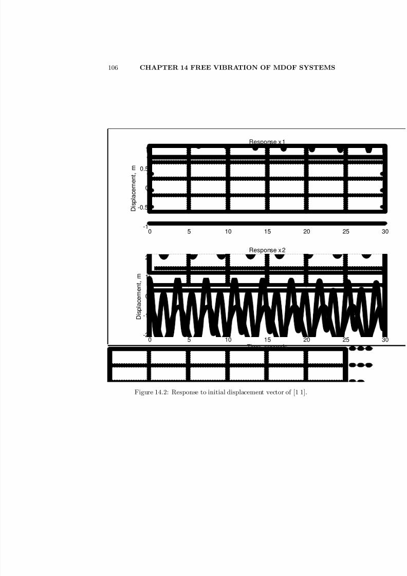
8/20/2019 Vibrations Using Matlab
http://slidepdf.com/reader/full/vibrations-using-matlab 111/170
106 CHAPTER 14 FREE VIBRATION OF MDOF SYSTEMS
0 5 10 15 20 25 -1
-0.5
0
0.5
1
D i s p
l a c e m e n t , m
Response x1
0 5 10 15 20 25 -2
-1
0
1
2
Time, seconds
D i s p l a c
e m e n t , m
Response x2
Figure 14.2: Response to initial displacement vector of [1 1].
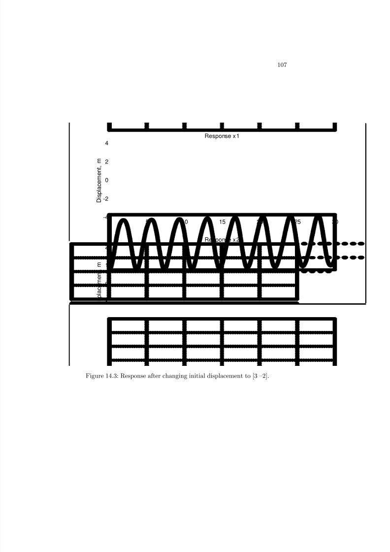
8/20/2019 Vibrations Using Matlab
http://slidepdf.com/reader/full/vibrations-using-matlab 112/170
107
0 5 10 15 20 25 30-4
-2
0
2
4
D i s p
l a c e m e n t , m
Response x1
0 5 10 15 20 25 30-2
-1
0
1
2
Time, seconds
D i s p l a c
e m e n t , m
Response x2
Figure 14.3: Response after changing initial displacement to [3 –2].

8/20/2019 Vibrations Using Matlab
http://slidepdf.com/reader/full/vibrations-using-matlab 113/170
108 CHAPTER 14 FREE VIBRATION OF MDOF SYSTEMS
0 5 10 15 20 25 -1
-0.5
0
0.5
1
D i s p
l a c e m e n t , m
Response x1
0 5 10 15 20 25 -0.2
-0.1
0
0.1
0.2
Time, seconds
D i s p l a c
e m e n t , m
Response x2
Figure 14.4: Response after changing initial displacement to [1 0].

8/20/2019 Vibrations Using Matlab
http://slidepdf.com/reader/full/vibrations-using-matlab 114/170
109
0 5 10 15 20 25 30-1
-0.5
0
0.5
1
Time, seconds
D i s p l a c
e m e n t , m
Response x2
0 5 10 15 20 25 30-2
-1
0
1
2
D i s p
l a c e m e n t , m
Response x1
Figure 14.5: Response after interchanging system masses.

8/20/2019 Vibrations Using Matlab
http://slidepdf.com/reader/full/vibrations-using-matlab 115/170
110 CHAPTER 14 FREE VIBRATION OF MDOF SYSTEMS
0 5 10 15 20 25 -2
-1
0
1
2
D i s p
l a c e m e n t , m
Response x1
0 5 10 15 20 25 -2
-1
0
1
2
Time, seconds
D i s p l a c
e m e n t , m
Response x2
Figure 14.6: Response with initial velocity [4 2] and initial displacement [1 1].
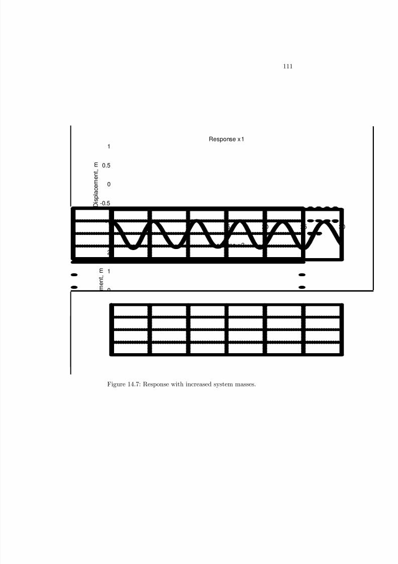
8/20/2019 Vibrations Using Matlab
http://slidepdf.com/reader/full/vibrations-using-matlab 116/170
111
0 5 10 15 20 25 30-1
-0.5
0
0.5
1
D i s p
l a c e m e n t , m
Response x1
0 5 10 15 20 25 30-2
-1
0
1
2
Time, seconds
D i s p l a c
e m e n t , m
Response x2
Figure 14.7: Response with increased system masses.

8/20/2019 Vibrations Using Matlab
http://slidepdf.com/reader/full/vibrations-using-matlab 117/170
112 CHAPTER 14 FREE VIBRATION OF MDOF SYSTEMS
0 5 10 15 20 25 -1
-0.5
0
0.5
1
D i s p
l a c e m e n t , m
Response x1
0 5 10 15 20 25 -2
-1
0
1
2
Time, seconds
D i s p l a c
e m e n t , m
Response x2
Figure 14.8: Response with reduced system sti¤nesses.

8/20/2019 Vibrations Using Matlab
http://slidepdf.com/reader/full/vibrations-using-matlab 118/170
Chapter 15
Damping of MDOF Systems
In the previous example, the free response of systems having more than one de-gree of freedom was discussed. Now, viscous damping is added to the system, asshown in Figure 15.1, and we will examine the changes caused by this addition.The equations of motion become:
m1::x1 + (c1 + c2)
:x1 c2
:x2 + (k2 + k1) x1 k2x2 = 0 (15.1)
m2::x1 + c2
:x2 :
x1
+ k2 (x2 x1) = 0: (15.2)
In matrix form, we obtain:
M ::x + C
:x + K x = 0;
where M =
24 m1 0
0 m2
35 ; C =
24 c1 + c2 c2
c2 c2
35 ; K =
24 k1 + k2 k2
k2 k2
35.
As we know, with damping present, there is no guarantee that the equationswill decouple by the procedure used earlier. However, for proportional damping,i.e., C = C mM + C kK; it is possible to follow the previous decoupling proce-
dure. This is because both K and M are diagonalized through the matrix of eigenvectors U . Thus, a scalar multiplied by M or K will also be diagonalized,and the sum of two diagonal matrices is also diagonal.
While proportional damping is something of a savior for modal analysis, itpresents a headache when programming. The only way to assure decoupledequations in a program is to specify C m and C k instead of entering the matrix
113

8/20/2019 Vibrations Using Matlab
http://slidepdf.com/reader/full/vibrations-using-matlab 119/170

8/20/2019 Vibrations Using Matlab
http://slidepdf.com/reader/full/vibrations-using-matlab 120/170
115
i = tan
1
q io!di:q io + i!diq io ; (15.6)
noting that q io and :q iorefer to the initial displacement and velocity in the modal
coordinate, respectively. Having obtained the solution for q(t); we then use thelast step of the modal analysis procedure to …nd x(t): Note that this methoduses the entire modal analysis procedure as if damping did not exist, and thenadds in the damping when solving for q i(t): The program at the end of thisexample, used to generate the …gures that follow, demonstrates this approach.
Figures 15.2 through 15.4 use m1 = 9; m2 = 1; k1 = 24; k2 = 3; 1 = 0:05;and 2 = 0:1: Figure 15.2 uses an initial displacement vector of x0 = [1 0]; andthe results show the e¤ect of the damping; the response gradually dies out. InFigure 15.3, an initial velocity of [3 2] is added, and the result is no increase
in the transient period (as expected), but an increase in amplitude. Finally,Figure 15.4 removes the velocity and changes the initial displacement to [2 1];and the result is a greater amplitude, but the same length of transient periodas Figure 15.3. In all three …gures, note that both responses show the e¤ects of multiple sinusoids, even though the …rst mass is much greater than the second.This is because the …rst sti¤ness is very large; this sti¤ness keeps the mass fromgaining too much velocity, and so the smaller mass can e¤ectively transfer itsmomentum to the larger.
Finally, Figure 15.5 changes the damping ratios to 1 = 0:07 and 2 = 0:03:The di¤erence between this …gure and Figure 15.2 is that here the responses havea greater amplitude and a larger transient period, due to the smaller dampingratios.

8/20/2019 Vibrations Using Matlab
http://slidepdf.com/reader/full/vibrations-using-matlab 121/170
116 CHAPTER 15 DAMPING OF MDOF SYSTEMS
Program 14-1: moddamp.m% This code solves n-degree of freedom damped
% vibration using the modal analysis techniques % of Section 7.6.3.%clear;M=input(’Enter the mass matrix: ’);[n,o]=size(M);if n~=o error(’M matrix must be square!’);end K=input(’Enter the sti¤ness matrix: ’);[n,o]=size(K);if n~=o error(’K matrix must be square!’);end % Giving the option to input damping via % modal damping ratios or through the multiplying % factors Cm and Ck.%fprintf(’Press 1 to enter modal damping ratios, ’)qz=input(’or anything else to enter Cm and Ck. ’);if qz==1for iz=1:nzeta(iz)=input([’Enter the damping for mode ’,num2str(iz),’: ’]);end else
fprintf(’Given that [c]=Cm[M]+Ck[K], ’);Cm=input(’Enter the factor Cm: ’);Ck=input(’Enter the factor Ck: ’);end qu=0;[u,l]=eig(K,M);% Using “eig” in this way allows us to subtract M*w^2 % from K, instead of I*w^2 (where I is the n by n identity % matrix).% The output from “eig” gives unit-length eigenvectors.% We need to scale them with respect to M.%for s=1:n
alfa=sqrt(u(:,s)’*M*u(:,s));u(:,s)=u(:,s)/alfa;end x0=input(’Enter the initial displacement column vector: ’);xd0=input(’Enter the initial velocity column vector: ’);tf=input(’Enter the …nal time: ’);
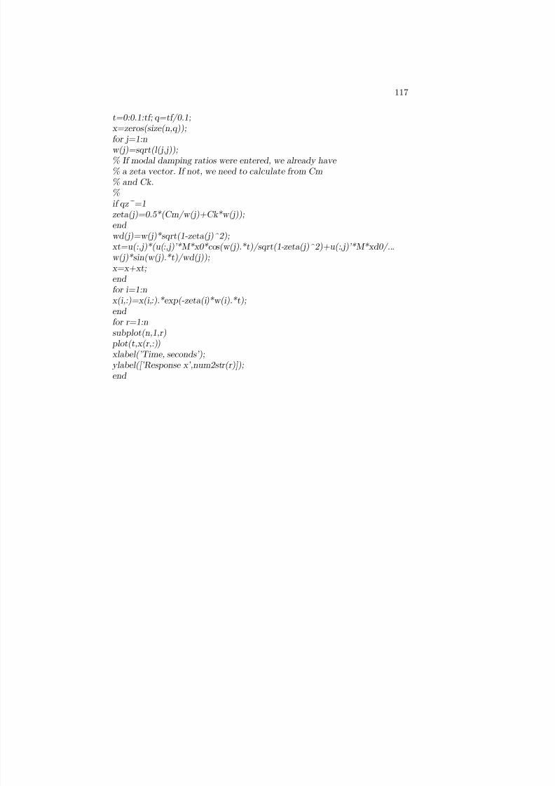
8/20/2019 Vibrations Using Matlab
http://slidepdf.com/reader/full/vibrations-using-matlab 122/170
117
t=0:0.1:tf; q=tf/0.1;x=zeros(size(n,q));
for j=1:nw(j)=sqrt(l(j,j));% If modal damping ratios were entered, we already have % a zeta vector. If not, we need to calculate from Cm% and Ck.%if qz~=1zeta(j)=0.5*(Cm/w(j)+Ck*w(j));end wd(j)=w(j)*sqrt(1-zeta(j)^2);xt=u(:,j)*(u(:,j)’*M*x0*cos(w(j).*t)/sqrt(1-zeta(j)^2)+u(:,j)’*M*xd0/...w(j)*sin(w(j).*t)/wd(j));x=x+xt;end for i=1:nx(i,:)=x(i,:).*exp(-zeta(i)*w(i).*t);end for r=1:nsubplot(n,1,r)
plot(t,x(r,:))xlabel(’Time, seconds’);
ylabel([’Response x’,num2str(r)]);end
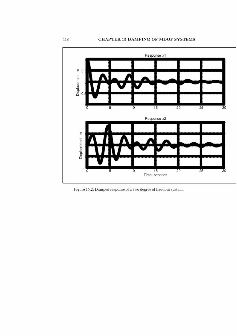
8/20/2019 Vibrations Using Matlab
http://slidepdf.com/reader/full/vibrations-using-matlab 123/170
118 CHAPTER 15 DAMPING OF MDOF SYSTEMS
0 5 10 15 20 25 -1
-0.5
0
0.5
1
D i s p l a c e m e n t , m
Response x1
0 5 10 15 20 25 -2
-1
0
1
2
Time, seconds
D i s p l a c e m e n t , m
Response x2
Figure 15.2: Damped response of a two degree of freedom system.

8/20/2019 Vibrations Using Matlab
http://slidepdf.com/reader/full/vibrations-using-matlab 124/170
119
0 5 10 15 20 25 30-2
-1
0
1
2
D i s p l a c e m e n t , m
Response x1
0 5 10 15 20 25 30-6
-4
-2
0
2
4
Time, seconds
D i s p l a c e m
e n t , m
Response x2
Figure 15.3: Response of a damped 2-DOF oscillator after adding an initialvelocity.

8/20/2019 Vibrations Using Matlab
http://slidepdf.com/reader/full/vibrations-using-matlab 125/170
120 CHAPTER 15 DAMPING OF MDOF SYSTEMS
0 5 10 15 20 25 -2
-1
0
1
2
D i s p l a c e
m e n t , m
Response x1
0 5 10 15 20 25 -4
-2
0
2
4
Time, seconds
D i s p l a c e m e n t , m
Response x2
Figure 15.4: Response of the same system to a di¤erent initial displacement.

8/20/2019 Vibrations Using Matlab
http://slidepdf.com/reader/full/vibrations-using-matlab 126/170
121
0 5 10 15 20 25 30-1
-0.5
0
0.5
1
D i s p l a c e
m e n t , m
Response x1
0 5 10 15 20 25 30-2
-1
0
1
2
Time, seconds
D i s p l a c e m e n t , m
Response x2
Figure 15.5: Response of the 2-DOF system with di¤erent modal damping ratios.

8/20/2019 Vibrations Using Matlab
http://slidepdf.com/reader/full/vibrations-using-matlab 127/170
8/20/2019 Vibrations Using Matlab
http://slidepdf.com/reader/full/vibrations-using-matlab 128/170
Chapter 16
A Universal Vibration
Solver
The next logical step in this sequence of examples would now be to introduceforcing functions of di¤erent types (as seen earlier with the single degree of freedom cases), and create several di¤erent programs. While this method ise¤ective, it is not e¢cient by any stretch of the imagination. The best way toproceed from here would be to create a program that solves all vibration cases,no matter what the forcing function or number of degrees of freedom.
The simplest way to go about this is to begin with a general program thatdoes not include the external force. Program 1, ndofold.m , demonstrates thismethod. Some techniques used in this program demonstrate ways to make aprogram modular. We need a general program to be as modular as possibleso that any changes that need to be made between runs of the program (likechanging the masses or the sti¤nesses) can be done without editing the code.The …rst major step in achieving this goal is the …rst line of the code. This lineassigns a variable to the number of degrees of freedom. This way, in any loopsor assignment statements made afterward, this variable can be referred to, andcan represent any number of degrees of freedom.
The next several lines initialize the variables needed later. This is done inlieu of a clear statement, because the clear statement will remove some variablethat will be needed later. Additionally, not using the clear command has theadvantage of allowing the user to assign variable names to the desired mass,sti¤ness, and other matrices. This way, when the program prompts for theselater, the user need only enter the variable name, not the entire matrix. If clear
is used, the matrices cannot be created beforehand. The trade-o¤ in not usingclear is that MATLAB must be told how large the matrices are to be; if thesesizes are not speci…ed, MATLAB will think the variables are to be the size thatthey are already. If we are now solving a three degree of freedom problem,and we had just previously solved a 2-DOF system, MATLAB will think themass matrix is to be 2 by 2. The …fth element entered would set o¤ an error
123
8/20/2019 Vibrations Using Matlab
http://slidepdf.com/reader/full/vibrations-using-matlab 129/170
124 CHAPTER 16 A UNIVERSAL VIBRATION SOLVER
message. The command used …lls each matrix with zeros; this is a harmless wayto initialize variables. Note how the variable n is used throughout this portion;
imagine the headache that would be involved if the program had not promptedfor n earlier. Each time an n appears, a change would have to be made to allowa di¤erent number of degrees of freedom to be analyzed.
After the initialization section, the program prompts for each matrix thatwill be needed. Having the necessary information, the program then solves thesystem by modal analysis, and prints out the output. Note how each calculationis done in loops that run from 1 to n. This maintains the generality of theprogram, allowing the user to specify with the …rst input how large the matriceswill be. Notice also that the plots are put up one at a time. This is donebecause there is no way to guarantee a subplot of any number of columns willbe readable. Imagine a forty degree of freedom system, and you will understandwhy a subplot cannot be guaranteed. So, the pause command is implementedafter each plot to allow the user to examine each plot to his satisfaction andto get a printout of the plot before the next one comes up (a printout canbe obtained from the graphics window in MATLAB for Windows only). Theprogram does not automatically print the graphs because they may be incorrector uninteresting, and to print them in such a case would be a waste of time andpaper. However, modifying the program to specify printing would take a fewseconds (replace pause with print in the code). Also, a loop could be created atthe beginning of the program to allow the user to specify whether output goesto the screen only, to a …le, to the printer, or to a combination of the three. Asample of such a loop follows here:
%This loop allows the user to specify the nature of the output.%Notice how the loop assumes that the user will enter the %wrong response; this is to correct for any mistakes, and
%to thwart those who love to crash programs.%Also, the program initializes the variable right before the loop%to the value necessary to continue the loop.outp=8;while outp==8
fprintf(’Enter 1 to print to the screen only, 2 to print to a …le, nn’)outp=input(’or 3 to print to the printer. ’);
%Notice how the text was split across two lines by using %the fprintf statement. This allows the text for input%statements to be as long as needed.%
if outp~=1&outp~=2&outp~=3
%Translation: “If outp isn’t equal to 1, 2, or 3.”%“~” means “not” for a MATLAB logical statement,%and the ampersand (&) is “and”, as usual.%This is where we let the user know he’s made a mistake.
fprintf(’Enter 1, 2, or 3!!!’)%Direct and to the point.
8/20/2019 Vibrations Using Matlab
http://slidepdf.com/reader/full/vibrations-using-matlab 130/170
125
%Now, outp is reset to the value needed to continue the
%loop, since we need the loop to continue.
%outp=8;
end
end
%One “end” for the “if”, and one for the “for”.%A common mistake is to leave one out, and then
%MATLAB tells you that it came to the end of the
%…le in the middle of a loop. (Not a pleasant feeling.)
So, there’s the loop! It’s not long (without the comments), and it’s e¤ective.It can be expanded as much as necessary to allow for any combination of printingoptions. One more thing: to get this to work, you need to put the following intothe printout loop (where the pause is now):
if outp==2
%“==” in MATLAB is “equals” to you and me.
print -dps …le1.ps elseif outp==3
elseif outp==1
pause
end
Note that if you type “else if” instead of “elseif”, MATLAB reads the “elseif” as a new if statement, needing its own end. Another common mistake.
Now, it’s just a matter of adding forcing functions to the mix. This task,however, is nearly impossible to do in a general way with the algorithm selected.So, we need to go back to the drawing board and …nd a simpler method. The…rst thing to realize is that the di¤erences among the several possible vibrationcases occur in solving the di¤erential equations. Every problem in vibrationsbegins as a set of second-order di¤erential equations, possibly coupled, possiblynot. Fortunately, MATLAB has the ode45 command, which solves di¤erentialequations numerically for a given time interval and initial conditions. Unfortu-nately, this command requires that the di¤erential equations exist in a functionM-…le which de…nes the system of di¤erential equations. Also, these di¤erentialequations must be …rst-order.
The problem of order is really not a di¢culty at all; there is a method bywhich a second-order di¤erential equation can be transformed into a system of 2
…rst-order equations. However, unless a general M-…le can be created, the userwould have to create his own function M-…le each time, which would then beused for ode45 . So then where would be the use of a program?
The answer lies in automating the process of creating an M-…le. MATLABhas …le transfer protocols, like any other programming language. We can write aprogram that tells MATLAB to create a speci…c M-…le from a general procedure

8/20/2019 Vibrations Using Matlab
http://slidepdf.com/reader/full/vibrations-using-matlab 131/170
126 CHAPTER 16 A UNIVERSAL VIBRATION SOLVER
we write into the program, and then solve the resulting system of di¤erentialequations with ode45. Program 2, ndof.m, performs this task.
Again, the program begins by specifying the number of degrees of freedomfor the run. The necessary matrices are initialized, and the inputs are obtained.After this, the program performs the …rst few steps of modal analysis, in orderto …nd the natural frequencies. We can do this because the natural frequenciesonly depend on the mass and sti¤ness matrices; we know that these can bedecoupled.
The next set of commands are initiated if a damping ratio matrix was en-tered. This loop changes the damping ratios into damping coe¢cients, by re-versing the modal analysis procedure. This can be done because the dampingratio vector that the user enters is related to the diagonal of the decoupleddamping coe¢cient matrix. Since this damping coe¢cient matrix is decoupled,it can be transformed from the modal coordinate system (the decoupled coor-dinate) back to the original coordinate system by applying the reverse of themodal analysis procedure.
Now that the program has the original values of the mass, sti¤ness, anddamping coe¢cient matrices, the M-…le can be created. The program …rstopens the …le with the fopen command. The strings in parentheses by thecommand specify the …lename, and the read/write privilege desired (‘w+’ means’write and overwrite,’ which allows a user of this program to make several runsin succession without erasing the M-…le previously created; the previous M-…leis lost). The fopen command is set equal to a variable because the commandspeci…es an arbitrary number by which MATLAB identi…es the …le. The onlyway to get this number is by setting fopen equal to a variable, so that thisnumber will be stored in an accessible place.
The reason that we need this identi…cation number is shown by the fprintf
statements that follow the fopen command. Each statement begins with the…le identi…cation number, so that MATLAB knows to write the text to the …lespeci…ed earlier, not to the screen. If the …le identi…cation number was not setequal to a variable, we would have no way to access it, and no way to write tothe …le.
Next, the functions de…ning the external forces on each degree of freedomare entered individually. This is necessary because a text string entered intoa MATLAB variable is stored one character per matrix element. So, if all theexternal forces were entered at once, there would be no way of telling how longthe force variable would be, or how many elements the matrix would have. Themethod used in the program avoids these di¢culties.
Notice the use of the num2str command within the fprintf statements. Thiscommand allows the value of a variable to be used in a text statement as text;
it is possible to use the value of a variable in an fprintf statement, but not astext. Note that to use the num2str command, the text to be printed must bewithin brackets as well as parentheses; this is because, if the brackets are notincluded, MATLAB thinks the statement ends when the quotes are closed, andwill produce an error instead of including the desired value of the variable.
Finally, the program uses an fclose statement to tell MATLAB that nothing
8/20/2019 Vibrations Using Matlab
http://slidepdf.com/reader/full/vibrations-using-matlab 132/170
127
else is to be entered into the …le. This is set equal to a variable, becauseMATLAB indicates a successful write transfer through the fclose statement;
a user can tell if the …le was written successfully by seeing the value of thisvariable.
Now, the program takes initial values necessary for ode45 , and solves. Theplots come printed individually; a print loop similar to the one described abovecan be inserted into this code to allow printing to a printer or to …les.
Figures 16.1 and 16.2 show the results of using ndof.m . Each …gure representsa degree of freedom of the system, whose parameters are as follows: m1 = 9;m2 = 1; c1 = 2:7; c2 = 0:3; k1 = 27; k2 = 3; F 1 = 0; F 2 = 3cos2t: Notice howeach degree of freedom shows the transient response over the …rst two seconds,and then settles into a steady-state response based on the single forcing function.The natural frequencies calculated by the program are !1 = 1:41 and !2 = 2:00;which match those calculated by hand. Also, the responses of each mode arefound through manual calculation to be:
x1(t) = 0:2451 cos(2t + 0:1974) 0:6249 sin(2t) (16.1)
x2(t) = 0:7354 cos(2t + 0:1974) + 1:8749 sin(2t): (16.2)
Looking at the maximum magnitudes of the responses shown in Figures 16.1and 16.2, we see that they are approximately equal to the sum of the coe¢cientsof the sine and cosine terms in the expression above, as we would expect. So,from this example, we see the power of the program and, more importantly,
verify that the program works.

8/20/2019 Vibrations Using Matlab
http://slidepdf.com/reader/full/vibrations-using-matlab 133/170
128 CHAPTER 16 A UNIVERSAL VIBRATION SOLVER
Program 16-1: ndofold.m%This program calculates the damped response of
%multi-degree of freedom systems without external forcing.%The user must enter the modal damping ratios; no other %method of describing damping is supported.n=input(’How many degrees of freedom are present? ’);m=zeros(n,n);k=zeros(n,n);s=zeros(n,n);
p=zeros(n,n);l=zeros(n,n);ac=zeros(1,n);
phi=zeros(1,n);m=input(’Enter the mass matrix. ’);ko=input(’Enter the sti¤ness matrix. ’);zeta=input(’Enter the damping ratio (zeta) matrix. ’);x0=input(’Enter the initial displacements. ’);xp0=input(’Enter the initial velocities. ’);ti=input(’Enter the initial time. ’);tf=input(’Enter the …nal time. ’);t=ti:(tf-ti)/1000;tf;[b1,b2]=size(t);x=zeros(n,b2);r=zeros(n,b2);a=m^(-1/2);kt=a*ko*a;[p,l]=eig(kt);
s=a*p;si=inv(s);r0=zeros(n,1);rp0=zeros(n,1);r0=si*x0’;rp0=si*xp0’;w=sqrt(l);wd=zeros(size(w));for k=1:n
wd(k,k)=w(k,k)*sqrt(1-zeta(k)^2);end %Note that the same loop control variable can be used for %every loop, so long as the loops are not nested within
%each other.for k=1:n
ac(k)=sqrt(wd(k,k)^2*r0(k)^2+(rp0(k)+zeta(k)*w(k,k)*r0(k))^2)/wd(k,k); phi(k)=atan2(wd(k,k)*r0(k),(rp0(k)+zeta(k)*w(k,k)*r0(k)));r(k,:)=ac(k)*exp(-zeta(k)*w(k,k)*t).*sin(wd(k,k)*t+phi(k));
end
8/20/2019 Vibrations Using Matlab
http://slidepdf.com/reader/full/vibrations-using-matlab 134/170
129
x=s*r;clg
for k=1:n plot(t,x(k,:))o=num2str(k);title([’Response x’,o])xlabel(’Time, seconds’)
ylabel(’Displacement’)grid …gure(gcf)
pause end for k=1:n
fprintf(’Natural frequency w%g=%g nn’,k,w(k,k))end Program 16-2: ndof.m%This program, as stated above, writes its own%M-…le to use in ode45. This algorithm allows %any external force combination to be examined,%and also allows the external force to be %a user-de…ned function.n=input(’How many degrees of freedom are present? ’);x=zeros(1,2*n);ct=zeros(n,n);m=input(’Enter the mass matrix. ’);aw=2;while aw==2
fprintf(’Press 0 to enter a damping coe¢cient matrix, or’)aw=input(’press 1 to enter a damping ratio (zeta) matrix. ’);if aw==0
c=input(’Enter the damping coe¢cient matrix. ’);elseif aw==1
zeta=input(’Enter the damping ratio matrix. ’);else
fprintf(’Please enter 0 or 1.’)aw=2;
end end k=input(’Enter the sti¤ness matrix. ’);a=m^(-0.5);
kt=a*k*a;[p,q]=eig(kt);omega=sqrt(q);if aw==1
for zt=1:nct(zt,zt)=zeta(zt)*2*omega(zt,zt);

8/20/2019 Vibrations Using Matlab
http://slidepdf.com/reader/full/vibrations-using-matlab 135/170
130 CHAPTER 16 A UNIVERSAL VIBRATION SOLVER
end af=a^(-1);
c=af*ct*af;end …d=fopen(’pdx.m’, ’w+’);fprintf(…d,’function pdx=pdx(t,x)nn’);for i=1:n
fprintf(…d,[’pdx(’,num2str(i), ’)=(-(’]);for j=1:n
if k(i,j)==0 else
fprintf(…d,[’(’,num2str(k(i,j)),’)*x(’,num2str(j+n),’)’]);end if c(i,j)==0 else
fprintf(…d,[’+(’,num2str(c(i,j)),’)*x(’,num2str(j),’)’]);end
end f=input([’Enter F’,num2str(i), ’(t) in quotes, like ‘3*cos(2*t)‘. ’]);fprintf(…d,[’)+(’,num2str(f),’))/(’,num2str(m(i,i)),’);nn’]);
end for i2=1:n
fprintf(…d,[’pdx(’,num2str(i2+n),’)=x(’,num2str(i2),’);nn’]);end status=fclose(…d);v0=input(’Enter the initial velocities as a row vector. ’);x0=input(’Enter the initial displacements as a row vector. ’);
ti=input(’What is your initial time? ’);tf=input(’What is your …nal time? ’);init=[v0,x0];[t,ny]=ode45(’pdx’,ti,tf,init);for kl=1:n
plot(t,ny(:,kl+n),’b’);title([’Response x’,num2str(kl)]);xlabel(’Time, seconds’);
ylabel(’Displacement, m’);grid …gure(gcf)
pause end
for l=1:nfprintf(’Natural frequency w%g=%g. nn’,l,omega(l,l))
end
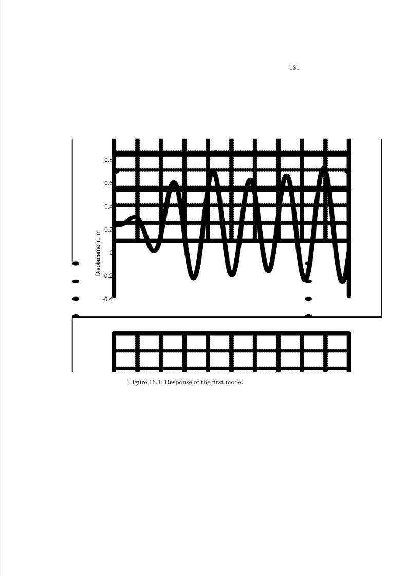
8/20/2019 Vibrations Using Matlab
http://slidepdf.com/reader/full/vibrations-using-matlab 136/170
131
0 2 4 6 8 10 12 14 16 18 20-0.8
-0.6
-0.4
-0.2
0
0.2
0.4
0.6
0.8
Time, seconds
D i s p l a c e m e n t , m
Response x1
Figure 16.1: Response of the …rst mode.

8/20/2019 Vibrations Using Matlab
http://slidepdf.com/reader/full/vibrations-using-matlab 137/170

8/20/2019 Vibrations Using Matlab
http://slidepdf.com/reader/full/vibrations-using-matlab 138/170
Chapter 17
Modeling a van der Pol
Oscillator
The next several examples will examine how we can use Matlab to solve formore real-world vibratory systems. The …rst such system we will look at isthe oscillatory motion of a structure surrounded by a ‡uid. Examples of suchstructures include the support pylons of o¤shore oil platforms and antennaeattached to the exterior surfaces of aircraft. These structures exhibit vibratorymotion due to the creation of vortices in the ‡uid by viscous interaction betweenthe structure and the particles comprising the ‡uid. Several investigators haveapplied the van der Pol equation,
•x + e x2 1 _x + x = 0; e > 0 (17.1)
as a model for the motion of such a structure. Note that this equation, giventhe positive parameter e; exhibits the usual form of damping when jxj < 1: How-ever, when jxj > 1; the term multiplying _x will become negative. If we were tosolve for •x; then, the damping term would add energy to the system, insteadof removing it. This negative damping approximates some of the phenomenaobserved in such ‡uid-structure interactions, and so is an attractive (and nec-essary) feature of the model. (The text gives a brief discussion of this problemas well, in Section 2.4.2.)
We will demonstrate how we can use Matlab to help us visualize the solutionto such a problem. First, we must solve the nonlinear ordinary di¤erentialequation given above. Unfortunately, we will not be able to arrive at an analyticsolution, as we did with several of the earlier problems we examined. What
we will be forced to do, then, is to integrate the equation analytically over aparticular time interval.
At …rst glance, it appears that we should be able to use a program likethe general solver in the previous example. This impression is correct, but touse such a program would be wasteful. Why would we use a program thatwas designed for a general case, having many varied inputs, when the only
133

8/20/2019 Vibrations Using Matlab
http://slidepdf.com/reader/full/vibrations-using-matlab 139/170
134 CHAPTER 17 MODELING A VAN DER POL OSCILLATOR
parameters we will have to use here are the parameter e, the initial conditions,and the time step?
The trouble then becomes, how are we going to allow the parameter e tobe dynamically assigned to the function in question? Our answer will comefrom Matlab’s global variable capability. We will also de…ne our van der Poloscillator solver as a function, so we can demonstrate another useful techniqueto generalize Matlab functions. We will make e_g into a global variable, so thatit can be passed freely between the main function and the function evaluatingthe van der Pol equation. (We will explain why we do not simply make e intoa global variable in a moment.) This is illustrated in the code below; Program1 is the main function, and Program 2 is the function used by ode45 to solvethe equation. We also introduce the nargin statement with this program. Thiscommand reads the input to the function, evaluating how many input argumentshave been passed into it (you can think of it as Number of ARGuments INput).We de…ne the function to take three inputs, but by using nargin, we allow asfew as zero inputs to be passed to the function, providing default values foreach input parameter. This allows our function to be quite ‡exible; if we’reonly interested in looking at the e¤ects of changing the parameter e; we neednot remember to pass in the same initial conditions and time span. We can usethe default values provided by the function in each case.
To assign these default values, we test the value of nargin three times. If this value is zero, the three if statements provide all of the default input data.If it is one, the function uses the default values for the initial state and the timespan. If the number of arguments is two, the function uses only the default timespan. (Experienced C programmers may be wondering why we chose three if
statements instead of a switch statement. The reader is invited to recast thenargin processing portion of this program to use the switch operator, and see
how the program changes.)Our trick to make this function work is to declare the parameter e_g asglobal. Note that there are two global statements in the programs below;one at the start of the main function, and one at the beginning of the functionused by ode45. Also note that there are no semicolons at the end of thesestatements; there is no output to suppress, so semicolons are unnecessary. Weare then able to use e_g in the subfunction as if it was assigned there, and not inthe parent function, after initializing e_g to the value of e: This construction isneeded because the function to be evaluated by ode45 must be a function of thestate and the time; adding in an extraneous third parameter will lead to errors.We could de…ne every variable we use as global, but that would uneccessarilyclutter the workspace with variables, and is considered poor technique. Globalvariables should be used with caution, as they allow parameters inside of a
function to be changed transparently (for example, we could write Program 2to adjust the value of e; e¤ectively defeating the input value). The bene…t of creating this van der Pol solver as a function is that the only variables created inthe workspace are the outputs t and x; not even the global variable e_g remainsin the workspace after function termination.
Now, why did we go to the trouble of introducing a spare parameter e_g to

8/20/2019 Vibrations Using Matlab
http://slidepdf.com/reader/full/vibrations-using-matlab 140/170
135
be our global variable? The answer comes from how Matlab handles its globalvariables. If you were to change e_g to e in the given code, you would …nd
no trouble for the default case (no input arguments). However, if you calledthe function with a speci…c value of e; Matlab would print a warning statementsaying that the value of your local variable (e) “may have been changed tomatch the global.” This is because Matlab sees the variable e that is input tothe function as a variable local to the function, and then sees the same variabledeclared as global later. Since the tail end of the warning includes the ominousstatement “Future versions of Matlab will require that you declare a variable tobe global before you use that variable,” this author thinks it prudent to writehis code in a way that will be forward-compatible, where possible. That meansthat our global variables will not be used before they are declared. In general,we will set apart our global variables with a trailing “g,” like in the programbelow. The curious reader is encouraged to rewrite the code to use e as a globalparameter, generating the Matlab warning.
The two …gures below show some results for the default case (as de…nedin Program 1). Figure 17.1 shows a simple comparison of displacement versustime; we see oscillatory behavior. The other two …gures that follow are phase
diagrams 1 , which are plots with the velocity on the y-axis and displacement onthe x-axis. These diagrams are often used in studies of nonlinear and chaoticsystems, since they can clearly show the e¤ects of initial conditions on theresponse.
The key feature of Figure 17.2 is the closed loop. Note that the initial lo-cation is denoted by a circle, and the …nal state by a triangle. The closed loopmeans that the van der Pol system eventually settled down into oscillatory be-havior. We can prove to ourselves that a closed loop in phase space correspondsto an oscillating response by considering the function x = sin(t) : If we take
this (obviously oscillating) function as our displacement, then the velocity isdescribed by y = cos(t) : If we were to plot this result in phase space, we wouldarrive at a circle; these functions x (t) ; y (t) are parametric equations for a circle.The van der Pol oscillator’s loop is not precisely circular, so it is not periodicin the same regular way as the sine or cosine function. However, it will repeatthe same sets of positions and velocities.
Figure 17.3 is the same default system with di¤erent initial conditions;we used the command [t; x] = solvevdp (0:5; [1; 5]) : Again, this initial point([1; 5]) is denoted by a circle, and the …nal point by a triangle. Note that, inspite of the di¤erent initial conditions, the motion settles into the same limitcycle. Thus, the limit cycle is determined by the parameter e; and not by theinitial conditions. This limit cycle behavior is similar to a phenomenon seen inthe vibration of structures in a moving ‡uid; thus, several investigators have
used the van der Pol equation to describe these systems. The reader is encour-aged to try di¤erent initial conditions to see that the limit cycle is indeed auniversal of the system.2
1 Also called phase portraits by some authors.2 However, changing the parameter e will certainly change the form of the limit cycle in

8/20/2019 Vibrations Using Matlab
http://slidepdf.com/reader/full/vibrations-using-matlab 141/170
136 CHAPTER 17 MODELING A VAN DER POL OSCILLATOR
function [t,x]=solvevdp(e,x0,tspan)% Program 1: solvevdp.m
% This function takes in a value for e in the % van der Pol oscillator expression,% x”+e(x^2-1)x’+x=0, where primes denote % di¤erentiation in time. The function% will automatically assume x(0)=1, x’(0)=0 % and a thirty-second time interval (tspan=[0 30])% if these values are not provided. Also, a % value of e=0.5 is assumed if none is given.global e_g if nargin<1 e=0.5; end % An “if” statement on a single line.if nargin<2 x0=[1 0]; end if nargin<3 tspan=[0 30]; end e_g=e;%% O¤ to the ode solver.%[t,x]=ode45(’dxvdp’,tspan,x0);function dx=dxvdp(t,x);
global e_g % Program 2: dxvdp.m% This is the function called on by ode45 to provide the % derivative of our state vector x. We need to set up the % second-order di¤erential equation as a system of two % …rst-order equations. Our state vector x consists of
% the variable x and its time derivative.%dx(1,1)=x(2);dx(2,1)=-(e_g*(x(1)^2-1)*x(2)+x(1));
phase space.
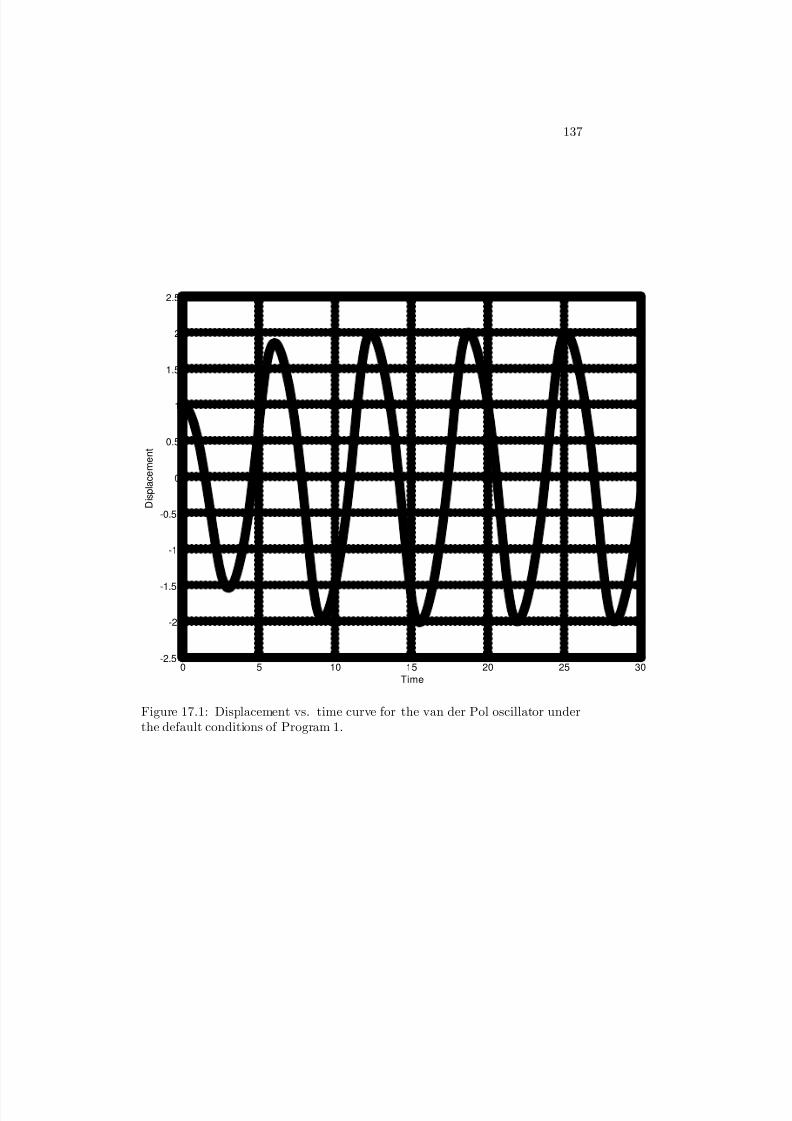
8/20/2019 Vibrations Using Matlab
http://slidepdf.com/reader/full/vibrations-using-matlab 142/170
137
0 5 10 15 20 25 30-2.5
-2
-1.5
-1
-0.5
0
0.5
1
1.5
2
2.5
D i s p l a c e m e n t
Time
Figure 17.1: Displacement vs. time curve for the van der Pol oscillator underthe default conditions of Program 1.
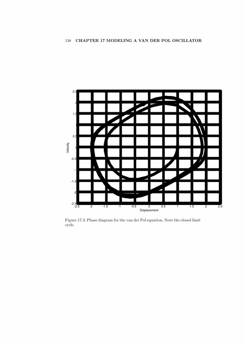
8/20/2019 Vibrations Using Matlab
http://slidepdf.com/reader/full/vibrations-using-matlab 143/170
138 CHAPTER 17 MODELING A VAN DER POL OSCILLATOR
-2.5 -2 -1.5 -1 -0.5 0 0.5 1 1.5 2 2.5-2.5
-2
-1.5
-1
-0.5
0
0.5
1
1.5
2
2.5
V e l o c i t y
Displacement
Figure 17.2: Phase diagram for the van der Pol equation. Note the closed limitcycle.
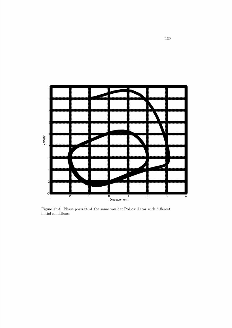
8/20/2019 Vibrations Using Matlab
http://slidepdf.com/reader/full/vibrations-using-matlab 144/170
139
-3 -2 -1 0 1 2 3 4-3
-2
-1
0
1
2
3
4
5
6
V e l o c i t y
Displacement
Figure 17.3: Phase portrait of the same van der Pol oscillator with di¤erentinitial conditions.

8/20/2019 Vibrations Using Matlab
http://slidepdf.com/reader/full/vibrations-using-matlab 145/170
8/20/2019 Vibrations Using Matlab
http://slidepdf.com/reader/full/vibrations-using-matlab 146/170
Chapter 18
Random Vibration and
Matlab
The focus in the text is probabilistic modeling of forces in vibrating systems.Our aim here is to show how Matlab can be used as an aid in modeling randomprocesses, and thus in visualizing the response of systems subjected to randomforcing.1 The logical starting point for this e¤ort is to show how we can createrandom forcing histories to apply to a deterministic model. Unlike the problemsposed in the text, we will not be looking for the response statistics at this time;instead, we will arrive at sample response realizations, which we will later use toarrive at the response statistics numerically, contrasting the analytic approachtaken in the chapter.
To illustrate some of the challenges associated with a random forcing input,
let us look at a sinusoidal forcing input of the form F (t) = A cos(!t) : We …rstneed to determine how we will introduce randomness to this system. That is,will we apply a random force amplitude, a random frequency, or both? If we aremodeling a given physical system, we will …nd that this question often answersitself. For example, we may have derived the power spectral density of a typicalinput to our system, and found that the vast majority of the energy input tothe system comes at one particular frequency. For this case, we could then (asa …rst approximation) treat the forcing frequency as deterministic, and use arandom distribution for the amplitude.2
Having determined the parameter we will consider to be random, we need toarrive at a probability density function for our this parameter. That is, will weuse a uniform distribution, a Gaussian distribution, or some other description?
Before we decide this, let us have a look at the distributions available insideMatlab.
1 Following the example of the textbook, we will limit ourselves mainly to random forcingof deterministic systems.
2 In general, we would also have a random phase angle associated with this forcing. Weomit the phase angle here for simplicity of analysis.
141
8/20/2019 Vibrations Using Matlab
http://slidepdf.com/reader/full/vibrations-using-matlab 147/170
142 CHAPTER 18 RANDOM VIBRATION AND MATLAB
The uniform and Gaussian distributions are built into Matlab through therand and randn commands, respectively.3 Typing a=rand(n) at the Matlab
prompt will return an n n array of randomly-generated numbers in a; usinga uniform distribution on the interval [0.0,1.0]. The randn command returnsa random number from a Gaussian distribution having a mean of zero andstandard deviation of one. Note that Matlab’s random numbers are actually“pseudo-random”; that is, they depend on an initial state vector. For someapplications, we will want to compare the results of several di¤erent systems toa random loading. For instances like this, we can use the state of the randomnumber generator to subject each comparison case to the same realization of therandom loading process. If we want to ensure that we get a di¤erent realizationeach time, we can use the suggestion available in the Matlab help for rand,and initialize the state to sum(100*clock). This will reset the random numbergenerator based on the current time.4 Both methods are useful for di¤erentcases. Any other probability distributions would have to be derived from thetwo described above or created from scratch by the user.
Following the lead of Section 4.8, let us look at the system described by
•x + 2!n _x + !2nx = F (t) (18.1)
where we will take F (t) to be the sinusoid above having random amplitudeA (t) : It will be convenient for us to apply the condition of ergodicity to thissystem. Thus, we will solve for the steady-state response only, neglecting thetransient response. (This also eliminates the need to specify initial conditions.)We can solve for the steady-state response in two ways using Matlab. We canuse the results of the analysis we did earlier, giving an analytic solution, or wecan use the numerical integration routines. We’ll do the latter in this case, to
show how we can transport the amplitude values back and forth where they areneeded, and to show how we can handle the discrete datapoint set.
Again, we use the nargin function to allow any number of input parametersfrom zero to the maximum of …ve. Recall from the last example that we used lessthan statements instead of a switch expression to de…ne parameters. This isbecause expression cases of a switch in Matlab do not require a break statementto end each expression set, unlike the C analogue. Thus, we cannot allow casesfor lower numbers of input arguments to “fall through” to higher numbers, likewe could in C. We also set the length of the amplitude vector A to be thesame as the length of the tspan vector, or 1000 elements if the input tspan isshorter. We do this to make interpolation of A based on values of t simpler.When Matlab integrates our di¤erential equation, the values of t that it will testare not necessarily the same as the values in tspan: Thus, we will interpolate
linearly between neighboring values of A corresponding to the two elements3 There also exist three other commands, two of which produce sparse matrices, while the
third gives a vector with a random permutation of the …rst n integers. These are not usefulto us here.
4 Speci…cally, the clock command returns a six-element vector, containing the current year,month, day, hour, minute, and second.

8/20/2019 Vibrations Using Matlab
http://slidepdf.com/reader/full/vibrations-using-matlab 148/170
143
of tspan that surround the current time value t:5 In order to ensure that theamplitude is always greater than zero, we multiply each element of A by its
sign. This leads to a distribution that is not rigorously Gaussian. We couldimprove our odds of not getting negative values for A by changing the standarddeviation such that 3 in each direction is positive. The coding for this is leftto the reader. The error expression in the default (otherwise) case of ourswitch expression will print the message in quotes to the screen, informing theuser of the function that the allowed values of the ‡ag are zero and one.
We are confronted with one more problem if we wish to use the di¤erentialequation solver. That is, how do we remove the transient response? It is not assimple as setting the initial conditions to zero, of course, since the position andvelocity imparted by the forcing function at time zero are not necessarily zero.What we must do is solve the di¤erential equation at time t = t0; and thensubstitute into the relation the values of the forcing and the forced response atthat time, to solve for the initial position and velocity required to match theforced response. Recall our earlier analysis, showing that x (t) = x p (t) + xh (t) ;where:
xh(t) = Ahe!t sin(!dt + ); (18.2)
andx p(t) = A0 (t)cos(!t ); (18.3)
where we found that the constants A0 and are:
A0 = A (t)q
(!2n !2) + (2!n!)2
; = tan1 2!n!
!2n !2
: (18.4)
We need to specify the initial conditions x (t0) and _x (t0) so that we can have
Ah = 0; eliminating the transient response xh (t) : This is as straightforward asspecifying x (t0) = x p (t0) and _x (t0) = _x p (t0) ; or:
x (t0) = A0 (t0)cos(!t0 )
_x (t0) = !A0 (t0)sin(!t0 ) : (18.5)
This is easily coded into Matlab, using the initial value of the force amplitudein the random array A: We neglect the time derivative of the randomly-varyingamplitude A as a …rst approximation. Figure 18.1 is the displacement versustime curve for the oscillation. The oscillation remains periodic even with therandom forcing amplitude, albeit with an irregular amplitude. The force ampli-tude is shown in Figure 18.2. The plot only shows the …rst …ve seconds to givea ‡avor for the variations in the force.
function [t,x,A]=randamp(tspan,wn,zeta,dist‡ag,omega);% Program 1: randamp.m% This program solves a single degree
5 This is a coarse approximation, to be sure, but has the bene…t of being simple to imple-ment. The reader is welcome to devise other re…nements.

8/20/2019 Vibrations Using Matlab
http://slidepdf.com/reader/full/vibrations-using-matlab 149/170
144 CHAPTER 18 RANDOM VIBRATION AND MATLAB
% of freedom oscillator given an% input of the form F(t)=Acos(omega*t+phi),
% where A is a random variable.% dist‡ag should be zero for uniform,% and 1 for Gaussian distribution.%global A_g tspan_g zeta_g wn_g omega_g phi_g % needed by the ode
de…nition.if nargin<1 tspan=linspace(0,30,1000); end if nargin<2 wn=1; end if nargin<3 zeta=0.05; end if nargin<4 dist‡ag=0; end if nargin<5 omega=3.5; end %% Assigning global values.%tspan_g=tspan; zeta_g=zeta;wn_g=wn; omega_g=omega; phi_g=0; % Zero phase angle.% Since we’ve got to have an amplitude for each% time step (ease of interpolation), we need to be speci…c % about how many time steps we’ve been given. We’ll say that if % tspan has fewer than 1000 elements, then we make % it a 1000-element vector.m=max(size(tspan));if m<1000 tspan=linspace(t(1),t(m),1000);
end
%% Now, we de…ne the amplitude A, between 0 and 5 for % the uniform distribution, and as a distribution with% mean of 2.5 for the Gaussian. We will force A>=0,% so the Gaussian distribution will need a little % bit of tweaking (and it won’t be rigorously Gaussian).%switch dist‡ag case 0 A=5*rand(size(tspan)); % A now has a range from 0 to 5.case 1A=2.5+randn(size(tspan)); % One standard deviation will span [1.5,3.5].A=A.*sign(A); % Multiplying A by the signum function of itself.
otherwise error(’Distribution ‡ag must be zero or one.’);
end %% Next, we de…ne the initial conditions to remove transients.%

8/20/2019 Vibrations Using Matlab
http://slidepdf.com/reader/full/vibrations-using-matlab 150/170
145
phi=atan(2*zeta*omega*wn/(wn^2-omega^2));x0=A(1)*cos(omega*tspan(1)-phi);
xd0=-A(1)*omega*sin(omega*tspan(1)-phi);xv0=[x0,xd0];%% Storing A in the global value.%A_g=A;%% Now we’re ready to solve the ODE.%[t,x]=ode45(’randdx’,tspan,xv0);function dx=randdx(t,x)%% Program 2: randdx.m% Di¤erential equation de…nition for % the randomly-varied amplitude case.%global A_g tspan_g zeta_g wn_g omega_g phi_g % Need these for the
interpolation.At=interp1(tspan_g,A_g,t); % Finding the correct value of A.% interp1 is a built-in function.%dx(1,1)=x(2,1);dx(2,1)=At*cos(omega*t-phi)-(2*zeta*wn*x(2,1)+wn^2*x(1,1));

8/20/2019 Vibrations Using Matlab
http://slidepdf.com/reader/full/vibrations-using-matlab 151/170
146 CHAPTER 18 RANDOM VIBRATION AND MATLAB
0 5 10 15 20 25 30-1
-0.5
0
0.5
1
1.5
Time, seconds
D i s p l a c e m e n t
Figure 18.1: Displacement versus time plot for the random Du¢ng oscillator.

8/20/2019 Vibrations Using Matlab
http://slidepdf.com/reader/full/vibrations-using-matlab 152/170
147
0 0.5 1 1.5 2 2.5 3 3.5 4 4.5 50
0.5
1
1.5
2
2.5
3
3.5
4
4.5
5
Time, seconds
A m p l i t u d e
Figure 18.2: Amplitude versus time curve for …ve seconds, to show variations.

8/20/2019 Vibrations Using Matlab
http://slidepdf.com/reader/full/vibrations-using-matlab 153/170

8/20/2019 Vibrations Using Matlab
http://slidepdf.com/reader/full/vibrations-using-matlab 154/170

8/20/2019 Vibrations Using Matlab
http://slidepdf.com/reader/full/vibrations-using-matlab 155/170
150CHAPTER 19 RANDOMLY-EXCITED DUFFING OSCILLATOR
Let us use the Du¢ng oscillator as a model for response to a harmonic input.Programs 1 and 2 below use the di¤erential equation solver suite inside Matlab
to calculate a numerical solution to a Du¢ng equation, given the input valuesof c; k; "; A; and !: The function uses g (x) = x2; this can be readily changedby editing the di¤erential equation de…nition function (Program 2). Also, thetime span and initial conditions are …xed inside the code, to keep the numberof inputs manageable. Program 1 can be quickly edited to take a di¤erent timeincrement or initial conditions, or to take them as function inputs. Figure showsthe results of the hard-coded default case.
Having arrived at a solution for the Du¢ng equation, our next step is tointroduce a random forcing function. Unlike the previous example (and inpreparation for the next) we will select a random forcing frequency and am-plitude, which will remain constant for the duration of the oscillation. If wedesign this function properly, we will not need to write a new program to pro-vide the di¤erential equation; we will send the same set of global variables. Thisimplementation is given in Program 3 below. Again, we leave the time intervaland initial conditions de…ned within the function. (The reader is encouraged torewrite the function to take the time increment, initial conditions, or both asinputs, providing default values via nargin.) We use the uniform distributiongenerator inside Matlab to provide a forcing amplitude between zero and 5, anda forcing frequency between zero and 2: Note that the function returns fourarrays: the time vector t, the state vector x; the random amplitude A; andthe random frequency w: This is for ease of comparison between runs, and alsomakes for a useful check on our random solution. Knowing the values of A andw used by the code, we can run our deterministic solver (Program 1) using thedefault values for e; c and k ; and the random values for A and w: The resultsfor a few default runs are plotted below, along with the random frequency and
amplitude used. Of special note is the third run in Figure 19.3. It happenedthat we got lucky (or unlucky, depending on the point of view) on this run, andgot a random forcing frequency very close to the system’s natural frequencyof one. Hence, we see a nearly-resonant condition in this undamped oscillator.The phase diagram in Figure 19.4 corresponds to this run. The response tracesout arcs in the phase plane that are circular, but by no means closed. Exam-ining the plot point by point shows that the oscillation travels back and forththrough the phase plane, meaning that the mean point of the oscillation doesnot move one way or the other; it is stationary at zero. The interested readeris encouraged to look at this behavior for himself. A simple way to accomplishthis is to run the Du¢ng oscillator function with the given parameters, and thentype the following at the Matlab prompt:
for i=1:max(size(x))
plot(x(i,1),x(i,2),’o’)hold on
pause end
Matlab will execute this loop as if it was inside a function or script, and you
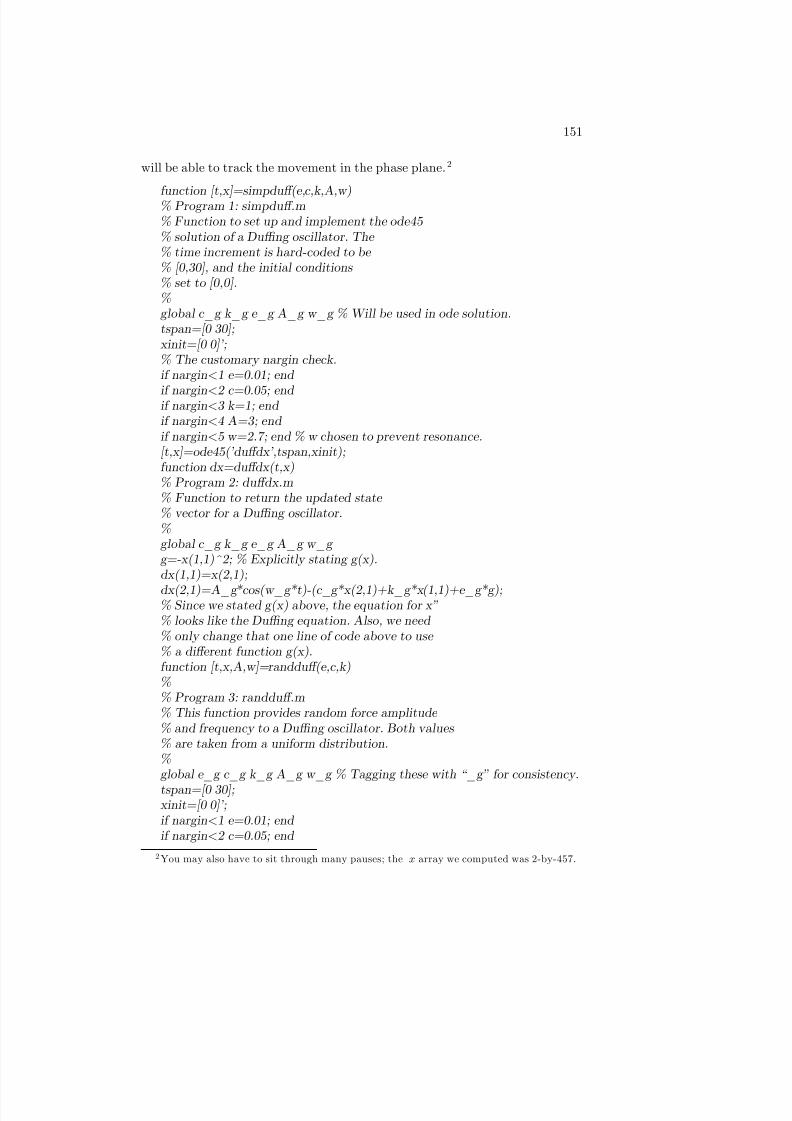
8/20/2019 Vibrations Using Matlab
http://slidepdf.com/reader/full/vibrations-using-matlab 156/170
151
will be able to track the movement in the phase plane.2
function [t,x]=simpdu¤(e,c,k,A,w)% Program 1: simpdu¤.m% Function to set up and implement the ode45 % solution of a Du¢ng oscillator. The % time increment is hard-coded to be % [0,30], and the initial conditions % set to [0,0].%global c_g k_g e_g A_g w_g % Will be used in ode solution.tspan=[0 30];xinit=[0 0]’;% The customary nargin check.if nargin<1 e=0.01; end
if nargin<2 c=0.05; end if nargin<3 k=1; end if nargin<4 A=3; end if nargin<5 w=2.7; end % w chosen to prevent resonance.[t,x]=ode45(’du¤dx’,tspan,xinit);function dx=du¤dx(t,x)% Program 2: du¤dx.m% Function to return the updated state % vector for a Du¢ng oscillator.%global c_g k_g e_g A_g w_g g=-x(1,1)^2; % Explicitly stating g(x).dx(1,1)=x(2,1);
dx(2,1)=A_g*cos(w_g*t)-(c_g*x(2,1)+k_g*x(1,1)+e_g*g);% Since we stated g(x) above, the equation for x”% looks like the Du¢ng equation. Also, we need % only change that one line of code above to use % a di¤erent function g(x).function [t,x,A,w]=randdu¤(e,c,k)%% Program 3: randdu¤.m% This function provides random force amplitude % and frequency to a Du¢ng oscillator. Both values % are taken from a uniform distribution.%global e_g c_g k_g A_g w_g % Tagging these with “_g” for consistency.tspan=[0 30];xinit=[0 0]’;if nargin<1 e=0.01; end if nargin<2 c=0.05; end
2 You may also have to sit through many pauses; the x array we computed was 2-by-457.

8/20/2019 Vibrations Using Matlab
http://slidepdf.com/reader/full/vibrations-using-matlab 157/170
152CHAPTER 19 RANDOMLY-EXCITED DUFFING OSCILLATOR
if nargin<3 k=1; end rand(’state’,sum(clock*100)); % Resetting random generator state.
A=5*rand(1);w=2*pi*rand(1);e_g=e; c_g=c; k_g=k; A_g=A; w_g=w;[t,x]=ode45(’du¤dx’,tspan,xinit);

8/20/2019 Vibrations Using Matlab
http://slidepdf.com/reader/full/vibrations-using-matlab 158/170
153
0 5 10 15 20 25 30-0.8
-0.6
-0.4
-0.2
0
0.2
0.4
0.6
Time, seconds
A m p l i t u d e
Figure 19.1: Response of the randomly-excited Du¢ng oscillator with ! =3:7960 and A = 3:7999:

8/20/2019 Vibrations Using Matlab
http://slidepdf.com/reader/full/vibrations-using-matlab 159/170
154CHAPTER 19 RANDOMLY-EXCITED DUFFING OSCILLATOR
0 5 10 15 20 25 30-4
-3
-2
-1
0
1
2
3
4
Time, seconds
A m p l i t u d e
Figure 19.2: Response of the Du¢ng oscillator to amplitude A = 4:4531 andforcing frequency ! = 1:7404:
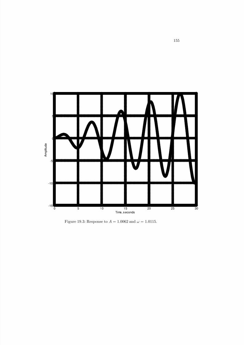
8/20/2019 Vibrations Using Matlab
http://slidepdf.com/reader/full/vibrations-using-matlab 160/170
155
0 5 10 15 20 25 30-15
-10
-5
0
5
10
Time, seconds
A m p l i t u d e
Figure 19.3: Response to A = 1:0062 and ! = 1:0115:

8/20/2019 Vibrations Using Matlab
http://slidepdf.com/reader/full/vibrations-using-matlab 161/170
156CHAPTER 19 RANDOMLY-EXCITED DUFFING OSCILLATOR
-1 -0.8 -0.6 -0.4 -0.2 0 0.2 0.4 0.6 0.8-2.5
-2
-1.5
-1
-0.5
0
0.5
1
1.5
2
2.5
Figure 19.4: Phase plot for the nearly-resonant case above.

8/20/2019 Vibrations Using Matlab
http://slidepdf.com/reader/full/vibrations-using-matlab 162/170
Chapter 20
Monte Carlo Simulation of
a Random System
In the previous example, we looked at a system under random excitation, wherewe modeled the amplitude of a harmonic input force as a time-varying ran-dom process, using a normal or uniform distribution. Consider now a relatedproblem, where we again have a harmonically-excited single degree of freedomoscillating system, where the excitation is of the form:
F (t) = A cos(!t) ; (20.1)
where the parameters A and ! are random variables. As with the previousanalysis, we assume that the forcing will be applied in a certain range, that is:
A1 A A2;
!1 ! !2 (20.2)
where A1; A2; !1; !2 are known constants. One approach would be to model theresults with A and ! at mean values, which could form a good basis to estimatethe behavior of a linear system. However, let us address the more interesting(and di¢cult) problem of estimating the behavior of a nonlinear system, such asthe Du¢ng oscillator from the previous example. There is no longer a guaranteethat the mean values for the inputs will correspond to the mean values of theresponse, so we need an alternate method to arrive at some response statistics. 1
To approximate the statistics of our nonlinear system, we choose to em-ploy the Monte Carlo methodology, developed systematically by Metropolis and
Ulam (1949). In general, the Monte Carlo method has two forms: the proba-bilistic form, where actual random variable distributions are available, and the
1 In addition to the numerical approach presented here, one can apply perturbation theoryto a nonlinear system to estimate the response. For more, see Nonlinear Ordinary Di¤erential
Equations , by D.W. Jordan and P. Smith (Oxford University Press), or A First Look at
Perturbation Theory, by J. G. Simmonds and J. E. Mann, Jr. (Dover Books).
157

8/20/2019 Vibrations Using Matlab
http://slidepdf.com/reader/full/vibrations-using-matlab 163/170

8/20/2019 Vibrations Using Matlab
http://slidepdf.com/reader/full/vibrations-using-matlab 164/170
159
a for loop to run the ODE solver the speci…ed number of times, solving for theappropriate initial displacement and velocity for each. After the ode solution is
found, the maximum displacement and velocity is found and stored, as are theinput amplitude and frequency, and the time span used. We may then performwhatever statistical analyses we wish on this data.
The four histograms below show the variations in several parameters for a setof 100 random realizations of the Du¢ng oscillator. Figure 20.1 is the histogramof force amplitudes, and Figure 20.2 is the set of forcing frequencies. Since wechose uniform distributions for both of these quantities, we expect the numberof values in each range to be about the same. This is the case; the di¤erencebetween the most and least common force amplitude range is eight occurrences,and the di¤erence between the most and least common frequency range is tenoccurrences. For a larger sample size, we would expect these numbers to reduceon a percentage basis.3
Our results, however, are not uniformly distributed. Figure 20.3 shows thevariation of maximum displacement values. The vast majority (65%) had max-imum displacement under 10. The shape of the distribution is akin to a one-sided Gaussian distribution, implying that our normally-distributed inputs ledto Gaussian output. Figure 20.4 also shows a one-sided Gaussian distribution,with 85% of the resulting maximum velocities falling under 10. One can readilysee how this information could be applied to a design procedure; if we wantedto have 90% certainty of a displacement less than 10, we would see that thedefault system is inadequate.
It is also possible to do more complicated analyses involving other aspectsof the data. The reader is invited to rewrite the routine to return all of thedisplacement and velocity histories (hint: three-dimensional matrices will behelpful). Also, if we had a nonlinear model for, say, a vibrating beam, we could
use the displacement and velocity information to derive the maximum stress atsome point in the beam for each run. The possible applications of this analysisare limited only by the systems we wish to apply it to.
function [xout,xdout,Aout,wout]=montdu¤(nruns,e,tspan)%% Program 1: montdu¤.m% This code performs a Monte Carlo simulation of the % Du¢ng oscillator. The random parameters are the % forcing amplitude and frequency, presumed to be % described by uniform distributions. Also, the % sti¤ness is presumed to be one and the damping % presumed to be 0.1. These values can be changed
% by editing the code.%global c_g k_g A_g w_g e_g % For compatibility with the existing du¤dx.m.
3 A test performed with 1,000 simulations showed that the di¤erence in amplitude oc-curences was 30 of 1000 between most and least common, or 3%. The di¤erence in numberof occurences for the most and least common frequency was also around 30 out of 1000.

8/20/2019 Vibrations Using Matlab
http://slidepdf.com/reader/full/vibrations-using-matlab 165/170
160CHAPTER 20 MONTE CARLO SIMULATION OF A RANDOM SYSTEM
% Parameter check.%
if nargin<1 nruns=50; end if nargin<2 e=0.01; end if nargin<3 tspan=[0 30]; end %% Sti¤ness and damping coe¢cient.%c_g=0.1; k_g=1; e_g=e;wlo=0; whi=2*pi; % Extreme values for the frequency.Alo=0.1; Ahi=10; % Extreme values for the amplitude.A=Alo+(Ahi-Alo)*rand(1,nruns);w=wlo+(whi-wlo)*rand(1,nruns);%% Initializing the t and x vectors. This is why we want% to specify the length of the time vector.%xout=zeros(1,nruns);xdout=zeros(1,nruns);for i=1:nruns A_g=A(1,i); w_g=w(1,i); % Set global parameters.x0=A_g*cos(w_g*tspan(1));xd0=-A_g*w_g*sin(w_g*tspan(1)); % Choose initial conditions to remove
transient.xinit=[x0, xd0];[trecv,xrecv]=ode45(’du¤dx’,tspan,xinit); % The run.xout(1,i)=max(xrecv(:,1)); % Here we could perform a more complex analy-
sis xdout(1,i)=max(xrecv(:,2)); % of our data.end wout=w;Aout=A;

8/20/2019 Vibrations Using Matlab
http://slidepdf.com/reader/full/vibrations-using-matlab 166/170
161
0 1 2 3 4 5 6 7 8 9 100
2
4
6
8
10
12
14
16
Force Amplitudes
N u m b e r o f O c c u r e n c e s
Figure 20.1: Histogram showing the force magnitudes among the 100 randomruns.
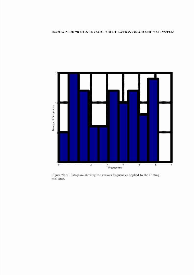
8/20/2019 Vibrations Using Matlab
http://slidepdf.com/reader/full/vibrations-using-matlab 167/170
162CHAPTER 20 MONTE CARLO SIMULATION OF A RANDOM SYSTEM
0 1 2 3 4 5 6 70
5
10
15
Frequencies
N u m b e r o f O c c u r e n c e s
Figure 20.2: Histogram showing the various frequencies applied to the Du¢ngoscillator.
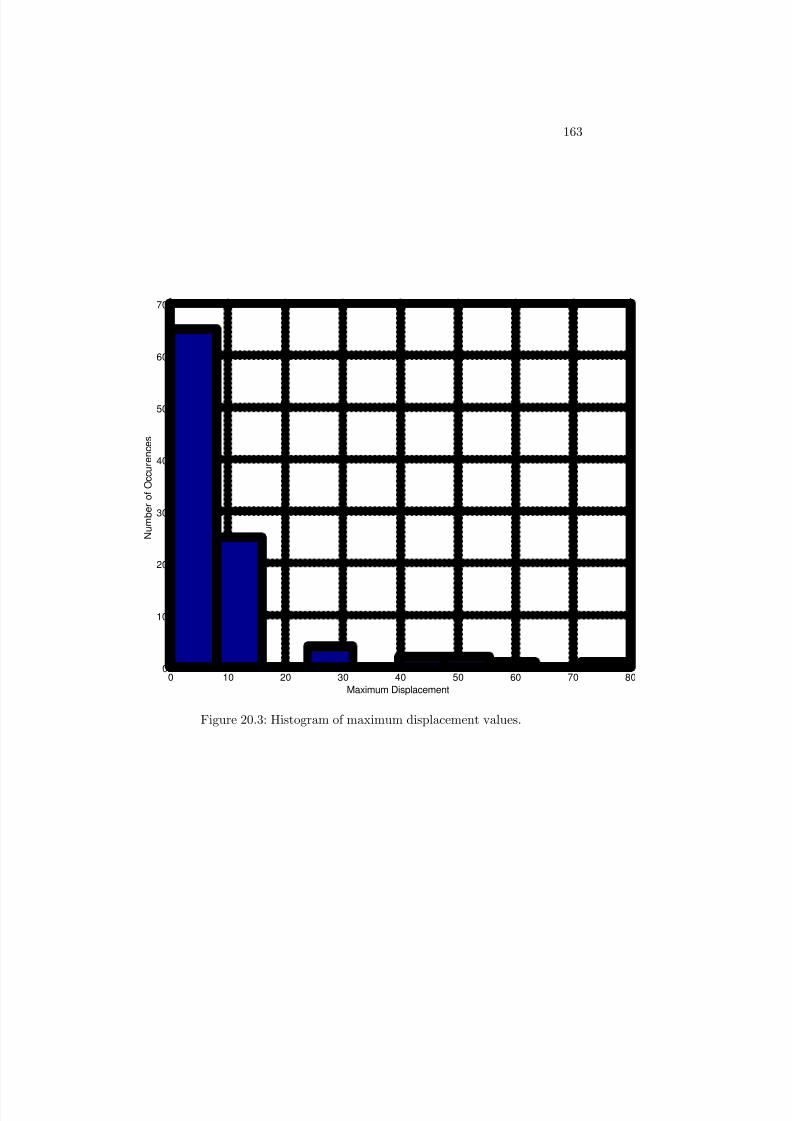
8/20/2019 Vibrations Using Matlab
http://slidepdf.com/reader/full/vibrations-using-matlab 168/170
163
0 10 20 30 40 50 60 70 800
10
20
30
40
50
60
70
Maximum Displacement
N u m b e r o f O c c u r e n c e s
Figure 20.3: Histogram of maximum displacement values.

8/20/2019 Vibrations Using Matlab
http://slidepdf.com/reader/full/vibrations-using-matlab 169/170
164CHAPTER 20 MONTE CARLO SIMULATION OF A RANDOM SYSTEM
0 10 20 30 40 50 600
5
10
15
20
25
30
35
40
45
Maximum V elocity
N u m b e r o f O c c u r e n c e s
Figure 20.4: Histogram showing maximum velocities of the simulated responses.

8/20/2019 Vibrations Using Matlab
http://slidepdf.com/reader/full/vibrations-using-matlab 170/170
Chapter 21
Conclusion
This primer on MATLAB as applied to vibration problems, simple and not sosimple, can be an valuable tool to the student and the practitioner. The basicelements are here to study a variety of vibration problems and to “play” withthe equations and the parameters. You will …nd it interesting and fun doingthis. Best of luck.