Vibrational Spectroscopy and Normal Mode Analysis

Applied to Human Prion Protein E200K:

Modeling The Effects of Targeted Microwave Radiation

New Mexico

Supercomputing Challenge

Final Report

April 1, 2009

Team 95

Sandia Preparatory School

Team Members

Jeff Fenchel

Christopher Parzyck

Evan Hughes

Teacher Sponsor

Neil McBeth

Project Mentor

Mark Fleharty

2

Table of Contents

Executive Summery—3

Prion E200K—4

Project Goal—5

One Dimensional Springs—6

Three Dimensional Spring Forces—9

Working With the Hessian—12

Simple Springs, Angular Springs, Torsion Springs—13

Covalent and Ionic Bonds—15

Non-Bonded Interactions—16

Lennard-Jones Potential and the Electrostatic Term—18

The Final Form of “k”—19

Resonance and Problems With the Model—21

The Carbon Dioxide Example—22

The Computer Model: Tinker—25

Program Flow—25

Minimizing the Protein—26

Finding Ideal Vibrational Modes—27

Prion Vacuum Simulation—28

Prion Water Box Simulation—28

Analysis Methods—32

Results—34

Thanks!—37

Bibliography—37

Code - 38

3

4

Executive Summary

The basis of our project is the excitation of normal modes of the human prion

protein E200K (Protein Data Bank index 1FKC) in order to change its structure. The

E200K prion has been linked to Creutzfeldt-Jakob disease, an incurable disease of the

human brain. This protein is a mutated from of a protein normally found in the human

body; the E200K variant transforms the normal state prion into another disease state

protein and, in the process, causes neural degradation. This disease-prion relies heavily

on the distribution of electric charges on its surface to latch onto and transform other

prions. It was our hope to find a way to neutralize E200K prions with specific

frequencies of microwave radiation by changing the molecular structure and thus surface

charge distibution. Our program, in conjunction with the molecular modeling package

TINKER, uses normal mode analysis to find the fundamental frequencies at which the

E200K prion vibrates. We then modeled how the structure of the prion protein changed

when it was bombarded with microwaves at the lower end of the molecule‟s fundamental

frequency spectrum. We used both graphical visualizations and mathematical techniques

to analyze the changes in molecular structure. We modeled the brief exposure of the

prion to microwave radiation in both a vacuum and water environment. We had great

success manipulating the E200K‟s structure in a vacuum but need to improve our

techniques for modeling the prion‟s transformation in a more realistic water environment.

The use of electromagnetic radiation to manipulate molecular structures holds great

promise for revolutionizing the field of medicine; our project aims to further explore

these possibilities and raise awareness about the theory and techniques involved with this

novel utilization of normal mode analysis and vibrational spectroscopy.

5

Prion E200K

The E200K prion protein causes Creutzfeldt-Jakob disease, an incurable illness,

by modifying the naturally produced PrPC

(prion protein) into the deadly pathogenic

conformer PrPsc

. PrPC

is naturally made in the human body. The disease state variant of

this protein, PrPsc

is created on the same gene codon but in a mutant state. Both of these

prion proteins have remarkably similar structures, except in the flexible regions. The

major differences are as follows: the PrPsc

has more Beta sheets, and the PrPc has more

alpha helixes, and the PrPsc

has a different electrostatic surface potential then the healthy

form. This means that the electric charges covering the surface of the protein are

arranged differently. Current research suggests that the proteins surface defects allow it

to seek out and attach to the PrPc variant. The E200K then acts like an enzyme,

changing the structure of the substrate prion and making one chemical change at the 200th

codon. During the mutation process the PrPsc replaces a negatively charged glutamic

acid with a positive charged lysine. This change results in the rapid transformation from

PrPc to PrP

sc. The loops and helixes of both of these prions are different. In one loop

region this is critical because it provides a building site for Protein X, which is thought to

be a crucial part in the transformation from PrPc to PrP

sc.

The PrPc utilizes these changes to covert healthy state prions to the disease state.

Once the PrPsc

is created it transforms other normal PrPc molecules into the disease state.

This means that the rate of reproduction of the prion begins slow if there are few original

E200K prions introduced, but accelerates rapidly after a long period of accumulation.

The disease can remain dormant for decades, making it even more deadly, for it

can be passed on by the same person multiple times before that person even realizes that

6

they have the disease, and by then his donated blood has been given to someone else. The

long incubation period is thought to be caused by the slow accumulation of PrPsc

. The

PrPsc

collects in the host‟s brain, slowly decaying it. Eventually creating holes in the

brain, and breaking down the nervous system, making Creutzfeldt-Jakob a spongiform

disease. The PrPc‟s

function is not fully understood but is believed to protect the brain

from dementia and other degenerative problems associated with by old age. When the

PrPc is contorted into a PrP

sc it further onsets these symptoms in the host.

Project Goal

Our project goal was to find a way to make this dangerous prion, E200K, inert.

There are currently no treatments for Creutzfeldt-Jakob disease and it is the most

common prion disease. In order to render the PrPsc

harmless the activation sites, crucial

for enzyme activity, must be rearranged in such a way that they are not functional. The

way we chose to do this was to utilize specific frequencies of microwave radiation to

cause the prion to vibrate and rearrange itself into a new form, where it cannot naturally

return to its disease state, by activating the normal modes of the molecule. The use of

electromagnetic waves to change the structure of proteins on the capsid of the Tobacco

necrosis virus by Arizona State University researchers Eric C. Dykeman and Otto F.

Sankey inspired our project. Their work is detailed in the essay Low Frequency

Mechanical Modes of Viral Capsids: An Atomistic Approach. Their work was much

more advanced and precise than ours, but utilizes many of the same basic principles.

What follows is a detailed walkthrough of how the fundamental frequencies of the prion

are found through normal mode analysis and then applied through vibrational

spectroscopy.

7

One Dimensional Springs

Vibrational spectroscopy, with regard to altering the physical structure of the

disease state form of the human prion protein E200K, is based on excitation of the

molecule through activation of the normal modes. The normal modes are frequencies the

molecule may vibrate at; they depend on both physical structure and forces acting both

inside the molecular structure and interactions with the molecule‟s surroundings. The

normal modes are derived using a combination of regular algebra, basic calculus, and

linier algebra. The following section describes a method for creating and solving the

matrix associated with normal mode analysis as well as an example modeling the simple

three atom molecule CO2.

To understand the derivation of normal modes it is not simplest to start on the

scale of the individual atom or molecule, but in classical macro-physics. Picture two

objects connected by a simple spring (one that obeys Hook‟s Law) with no outside forces

are acting on the system. If the objects are left to rest they will stay a fixed distance away

from each other—the spring will neither be extended past its rest length or contracted at

all. This state is called the minimized state of the system; this is because the potential

energy is at its minimal state. If an outside force pulls the two objects apart (extending

the spring) or pushes them together (compressing the spring) a force acts between the two

objects. The spring naturally wants to return towards its minimal state of energy and thus

its natural length. The force that acts between the objects is described by Hook‟s law:

F k x where F is force, k is the spring constant (also called the force constant) of the

spring adjoining the objects, and x is the change in length of the spring from its natural

length (if the original length of the spring is x0 and the new length is xn then

8

x x0 xn ). The negative sign means that the force is always the opposite the

direction that the spring has been altered—i.e. force has direction. The force constant, k,

represents the stiffness of the spring; if k is large the spring is hard to stretch, if k is small

the spring is easy to stretch. If the system is mechanically excited, the spring is stretched

or compressed, and there is no damping from outside forces then it will oscillate between

stretching and compressing at a fixed frequency until some outside force stops it. The

amount of time it takes the system to make one full cycle from the equilibrium point

(minimum potential energy) to maximum extension (maximum potential energy) to the

equilibrium point to maximum compression and back to the natural length is called the

period of the spring and is given byT 2 mk

. At all times the center of mass ( x ) of

the system remains constant. The frequency, or number of cycles per second, in Hertz

(Hz) is given as the reciprocal of the period. The potential energy of the system for any

amount of stretch is described by: e1

2 k( x)2 . Where

eis the potential energy.

Note that this expression is a quadratic equation with its vertex at the minimum potential

energy of the system. The first derivative of potential energy is the expression for force

e

xF k x

The second derivative of potential energy is the opposite of the force constant.

2

e

x2k

This is an important relationship that makes matters simple for the time being, but will

become more complicated later. The last point about the nature of the springs involves

the displacement with respect to time. As the spring‟s length changes its motion is

9

described by a sine curve. The displacement of either object from its original position

before excitation is given by the un-damped sine curve: s(t) Asin(2 vt) , where A is the

amplitude of motion (it depends on how much the spring was originally stretched and is

an arbitrary value for these calculations), v is the fundamental frequency of the system,

and t is time. For this system there is only one possible value of v but for more complex

systems there are a great many possible values—the calculation of all the possible values

of v for our molecule is the ultimate goal of this normal mode analysis. Taking the first

derivative of displacement, s(t), gives s '(t) (2 v)Acos(2 vt) . This represents the

velocity of the object at any given time. The second derivative of displacement gives the

acceleration with respect to time: s ''(t) (4 2v2 )( A)sin(2 vt) . The original expression

of displacement is substituted into the equation for acceleration to yield:

s ''(t) (4 2v2 )( s(t)) . Newton‟s second law of motion states that for any unbalanced

force on an object force equals mass times acceleration (F ma ). Multiplying both

sides of the expression by acceleration gives m[s ''(t)] ma F 4 2v2m[s(t)] . The

force created by the extension/compression of the spring is given as the derivative of

potential energy, e

xF k x . Setting the forces equal to each other gives

k x 4 2v2m[s(t)] . If the analysis of forces is not done with respect to time then the

expression s(t) is equivalent to x and the normal mode analysis equation becomes

k x1 4 2v2m2 x2 . What this equation really represents is: the resultant

displacement of object two due to the forces created by moving object one by some

amount. The resultant displacement is dependent on the frequency that the object is

moving at. Imagine the dual mass, single spring system again. If one mass is held still

10

while the other is moved and then the system is let go the second mass will be displaced

by the force from the spring resulting from the movement of the first mass. In a simple

one dimensional model like this one, the two displacements are equal and on the same

line by virtue of Newton‟s third law of motion. This system becomes much more

complicated when the objects are allowed to move in three dimensions.

Three Dimensional Spring Forces

Imagine, now, a cube, made up of eight masses at the points and each mass is

connected to every other mass by a simple spring. Disregard that, at the center of the

cube (and in the middle of each of the faces), the diagonal springs intersect each other;

the important property of the springs is this. They represent a variable force between

masses, their physical appearance is trivial. If any one of the masses is moved in any

direction the forces created by the springs will cause all the other masses to move in

various directions by various amounts. This is where the liner algebra aspect of normal

mode analysis comes in to play. First: the system of masses and springs is a three-

dimensional object in three-dimensional space, so all movement in space is broken down

into components. The movement of a mass, mn, from its minimized position (the

minimized state of the cube is, again, when the potential energy of the system is at its

lowest) is represented by sn . Note that s is boldface—this means that it represents a

vector, which has both direction and magnitude; in the earlier example x had only one

direction to represent so it was not written in boldface and only referred to magnitude.

sn can be broken down into unit vectors, one for each direction in x,y,z space:

sn xn yn zn . The unit vectors: xn, yn, and zn all represent distances along

the x,y, and z axis, respectfully, from the original position of the mass mn. Generally, at

11

this stage, all measurements of displacement are done so with the origin at the center of

mass of the system (internal Cartesian coordinates), which is at the center of the cube in

this case if all the objects are of equal mass. The center of mass with respect to any

outside coordinate system is (x,y, z ) .

So, if one mass is moved it will affect the position of every other mass, according

the equation derived earlier: k sb 4 2v2ma sa . This equation can be expanded

using knowledge of vectors.

kxxab

xb kxyab

yb kxzab

zb 4 2v2ma xa

kyxab

xb kyyab

yb kyzab

zb 4 2v2ma ya

kzxab

xb kzyab

yb kzzab

zb 4 2v2ma za

This system of equations deals with the movement of two objects—ma and mb in three

dimensions. mb is being moved by some outside force, this causes the spring connecting

it to ma to change length and produce a force, displacing ma by some amount. The left

hand side of this equation deals with how mb is being moved in space—in terms of x,y,

and z. The right side shows how that force will cause ma to be displaced. Note that the

force on the left side has nothing to do with the mass of the object being moved, only the

distance, whereas the force on the right side involves the mass of the object and the

frequency of the oscillation. Going back to the cube, to find all the possible ways that

one object can be moved, in each direction, the movements of every other object, in every

direction, must be considered. If the eight masses are called m1, m2,… mn … m8 where

1 n 8 and n . The system of equations describing the displacement of one atom:

m1 due to the displacement of any of the other atoms is:

12

kxx11

x1 kxy11

y1 kxz11

z1 kxx12

x2 kxy12

y2 kxz12

z1... kxx1n

xn kxy1n

yn kxz1n

zn 4 2v2m1 x1

kyx11

x1 kyy11

y1 kyz11

z1 kyx12

x2 kyy12

y2 kyz12

z1... kyx1n

xn kyy1n

yn kyz1n

zn 4 2v2m1 y1

kzx11

x1 kzy11

y1 kzz11

z1 kzx12

x2 kzy12

y2 kzz12

z1... kzx1n

xn kzy1n

yn kzz1n

zn 4 2v2m1 z1

Again the right sides of the equations represent the resultant displacement of one object

in the system, in this case object m1 in any direction. The left side of the equation

represents all the possible movements of all the other objects in the system in all

directions and the forces they induce. This system of equations can then be expanded

further, instead of looking at the resultant force and displacement of one object,

depending on all the objects, the system can represent the resultant force/displacement of

any object as a result of any movement of any other object, in any three dimensional

space. For the eight object, three-dimensional system described earlier where 1 n 8

and n the system of equations is:

kxx11

x1 kxy11

y1 kxz11

z1 kxx12

x2 kxy12

y2 kxz12

z1... kxx1n

xn kxy1n

yn kxz1n

zn 4 2v2m1 x1

kyx11

x1 kyy11

y1 kyz11

z1 kyx12

x2 kyy12

y2 kyz12

z1... kyx1n

xn kyy1n

yn kyz1n

zn 4 2v2m1 y1

kzx11

x1 kzy11

y1 kzz11

z1 kzx12

x2 kzy12

y2 kzz12

z1... kzx1n

xn kzy1n

yn kzz1n

zn 4 2v2m1 z1

kxx21

x1 kxy21

y1 kxz21

z1 kxx22

x2 kxy22

y2 kxz22

z1... kxx2n

xn kxy2n

yn kxz2n

zn 4 2v2m2 x2

kyx21

x1 kyy21

y1 kyz21

z1 kyx22

x2 kyy22

y2 kyz22

z1... kyx2n

xn kyy2n

yn kyz2n

zn 4 2v2m2 y2

kzx21

x1 kzy21

y1 kzz21

z1 kzx22

x2 kzy22

y2 kzz22

z1... kzx2n

xn kzy2n

yn kzz2n

zn 4 2v2m2 z2

kxxn1

x1 kxyn1

y1 kxzn1

z1 kxxn2

x2 kxyn2

y2 kxzn2

z1... kxxnn

xn kxynn

yn kxznn

zn 4 2v2mn xn

kyxn1

x1 kyyn1

y1 kyzn1

z1 kyxn2

x2 kyyn2

y2 kyzn2

z1... kyxnn

xn kyynn

yn kyznn

zn 4 2v2mn yn

kzxn1

x1 kzyn1

y1 kzzn1

z1 kzxn2

x2 kzyn2

y2 kzzn2

z1... kzxnn

xn kzynn

yn kzznn

zn 4 2v2mn zn

Note that this is a system of 3n equations in 3n variables ( x, y, z are the components

of one variable s , or displacement). Also important is the recursive nature of the

system—for each solution on the right for a displacement that is then re-substituted into

the equation for the corresponding displacement on the left. This system of equations is

rather unwieldy. A matrix is formed of all the force constants (i.e. the second derivatives

13

of potential energy). The original set of all the forces in a matrix is called the Force-

matrix or F-matrix, the matrix of all the second derivatives ofe is called the Hessian

matrix. By factoring out all of the x, y, z components the system becomes:

kxx11 kxy

11 kxz11 kxx

12 kxy12 kxz

12 ... kxx1n kxy

1n kxz1n

kyx11 kyy

11 kyz11 kyx

12 kyy12 kyz

12 ... kyx1n kyy

1n kyz1n

kzx11 kzy

11 kzz11 kzx

12 kzy12 kzz

12 ... kzx1n kzy

1n kzz1n

kxx21 kxy

21 kxz21 kxx

22 kxy22 kxz

22 ... kxx2n kxy

2n kxz2n

kyx21 kyy

21 kyz21 kyx

22 kyy22 kyz

22 ... kyx2n kyy

2n kyz2n

kzx21 kzy

21 kzz21 kzx

22 kzy22 kzz

22 ... kzx2n kzy

2n kzz2n

kxxn1 kxy

n1 kxzn1 kxx

n2 kxyn2 kxz

n2 ... kxxnn kxy

nn kxznn

kyxn1 kyy

n1 kyzn1 kyx

n2 kyyn2 kyz

n2 ... kyxnn kyy

nn kyznn

kzxn1 kzy

n1 kzzn1 kzx

n2 kzyn2 kzz

n2 ... kzxnn kzy

nn kzznn

x1

y1

z1

x2

y2

z2

xn

yn

zn

4 2v2

m1 x1

m1 y1

m1 z1

m2 x2

m2 y2

m2 z2

mn xn

mn yn

mn zn

The components are „factored‟ out into a separate matrix according to the rules of matrix

multiplication. If the matrices are multiplied out they form the system of equations in the

above step.

Working With the Hessian

Next the system is mass weighted to produce a more symmetric matrix. The

process seems to complicate the equation in the short term. It ultimately makes the

eigenvector/eigenvalue process simpler. The mass weighted coordinate system is based

on the identity:sn mn sn . This form is achieved by dividing all the displacement

entries of the matrix on the right-hand side of the equation by the square-root of the

corresponding mass term. When this is done to both sides of the equation, in order for

both sides to remain equal, each k value is divided by two square-root mass terms—the

14

affecting and affected objects. So kxxab kxx

ab

ma mb. This entire matrix, in the case of

the cube and 3(8)x3(8) or 24x24, can be written in the form of:

H kij and

k

kxxij

mi m j

kxyij

mi m j

kxzij

mi m j

kyxij

mi m j

kyyij

mi m j

kyzij

mi m j

kzxij

mi m j

kzyij

mi m j

kzzij

mi m j

H

kxxij

mi m j

kxyij

mi m j

kxzij

mi m j

kyxij

mi m j

kyyij

mi m j

kyzij

mi m j

kzxij

mi m j

kzyij

mi m j

kzzij

mi m j

ij

S

x1

y1

z1

xnynzn

HS 4 2v2 S 1 i n 1 j n

This then becomes the final form of the equation used for normal mode calculation. To

actually solve the secular equation and get the possible values of the fundamental

frequencies, or normal modes, a process called diagonalization is then used to derive the

eigenvalues and eigenvectors. This system is actually more complex then it appears,

further information is needed to fully comprehend it.

Simple Springs, Angular Springs, Torsion Springs

The whole basis of this system of equations and matrix relies on some

assumptions about the meaning of “k.” Earlier it was defined as the spring constant of a

simple, linear spring—or the second derivative of the potential energy stored in a spring.

This is fine for a very small and predominantly linear system; as the complexity of the

system increases, however, some other parts of the constant k must be considered. Take,

15

for instance, the cube discussed earlier. Every point is connected to every other object

with a spring that can compress and stretch in a linear fashion. Call the spring constant

associated with this stretch k . As the masses move around there is also some bending

of the angles between the springs. The angles will naturally want to return to their

equilibrium points. In the case of the cube all angles equal 90 degrees. Another form of

Hook‟s law applies to this situation. Instead of considering the „stretching energy‟ of the

spring, the „bending energy‟ is considered. If 0 is the angle of the springs in the

system‟s minimized position and is the new angle, after displacement of an object, then

the bending energy involved is given by: 1

2k ( 0 )2 . The second derivative of

this expression is:

2

2k

This yields another constant to be factored into the Hessian matrix. The values of k

represented in the matrix H are the sum of all the spring constants and partial derivatives

of all the forces acting between the objects. As far as springs go there is only one more

physical process to be explored: torsion. Not only can the lengths and angles between

objects change, but they can also rotate about an axis. Take, for example, one of the

faces of the cube. Call the square abcd . abc bcd and ab bc cd . If the mass,

a, is moved to the new position a’, but a bc abc bcd ( ba d bad ) and

a b ab bc cd then the angle a ba is the angle of rotation, or the angle of twist.

This idea works for any four object shape, if the angle between two planes, defined by

triangles made of three points on the perimeter of the shape, changes from its minimized

state then the system is considered to be a torsion spring. If the angle 0 is the original

16

position and is then new angle then the torsion energy stored is given as:

1

2k ( 0 )2

. The second derivative of torsional potential energy is -k . So far,

k ij k k k . For the most part, these are the only ways that macroscopic structures

can move around: stretch, bend, and twist. The ultimate goal, however, involves analysis

of forces on a microscopic scale.

Covalent and Ionic Bonds

Next, it is necessary to explore forces and force constants on the intermolecular

scale. In this case the objects are no longer just floating masses, but nuclei of atoms.

There are no springs attaching the nuclei to each other, instead there are electromagnetic

forces acting between all of them. Atoms can be attached to one another in one of two

ways; they can be bonded together due to interactions of electron clouds or they can

interact through non-bonded forces.

The two main groups of chemical bonds relevant to the human prion protein,

E200K, are covalent bonds and ionic bonds. Covalent bonds occur when two atoms

share a valence, or outer orbital, electron between them. The electron cloud spreads

between the two atoms and this holds them together. This sharing of electrons may be

even (pure covalent bonding) or uneven (polar covalent bonding). If the electron is

pulled so much by one atom away from another that it is considered to have „left‟ its

original nucleus then the bond is ionic. Covalent and ionic bonds are the strongest forces

that generally exist between two atoms in a molecule. Though the equations governing

the force between the two atoms are complex they are approximated with the three

macroscopic phenomena listed earlier. Within very short distances from the minimized

state of the molecule the bond forces are approximated very well with Hook‟s Law

17

(although the approximation breaks down over greater distances). So covalent, polar

covalent, and ionic bond interactions between atoms in the protein are dealt with by

summing the spring constants of stretching, bending, and twisting.

Non-Bonded Force Interactions

The nature of the atom, a positive charged nucleus surrounded by numbers of

negatively charged electrons, gives rise to additional internal molecular forces that must

be considered. These non-bonded interactions link every atom in the protein to every

other atom, as well as to any and all atoms in the environment, by way of longer-range

force fields. These forces are generally termed “van der Waals” forces after the Dutch

scientist Johannes Diderik van der Waals. This set of forces describes the interactions

between ions and neutral molecules (or segments of molecules). It contains both an

attractive (at long distances) and repulsive part (at shorter distances). The attractive

component of the van der Waals force field has three main components. The first, and

strongest, involves the interactions of two permanent multipoles. When two atoms are

bonded together and one has a higher electronegativity then the other the electron cloud is

unevenly distributed—creating a section of the molecule with a net positive ( ) charge

and a section with a net negative charge ( ). This is called a dipole moment. A

molecular section that has multiple dipole moments has a multipole. The unlike charged

sections of the molecule attract and the like charges repel (intramolecular force). These

multiple moments in a molecule, like a prion, also interact with the molecules

surrounding it (intermolecular force). The polarity of the sections of the molecule are

determined by the polar-covalent or ionic bonds acting. This is called a fixed dipole-

dipole van der Waals-Keesom force, sometimes referred to as a Hydrogen bond (or

18

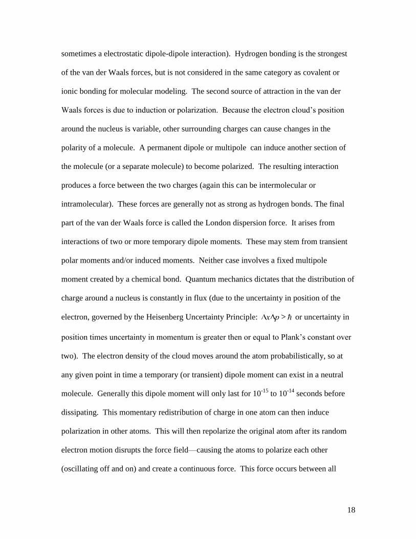
sometimes a electrostatic dipole-dipole interaction). Hydrogen bonding is the strongest

of the van der Waals forces, but is not considered in the same category as covalent or

ionic bonding for molecular modeling. The second source of attraction in the van der

Waals forces is due to induction or polarization. Because the electron cloud‟s position

around the nucleus is variable, other surrounding charges can cause changes in the

polarity of a molecule. A permanent dipole or multipole can induce another section of

the molecule (or a separate molecule) to become polarized. The resulting interaction

produces a force between the two charges (again this can be intermolecular or

intramolecular). These forces are generally not as strong as hydrogen bonds. The final

part of the van der Waals force is called the London dispersion force. It arises from

interactions of two or more temporary dipole moments. These may stem from transient

polar moments and/or induced moments. Neither case involves a fixed multipole

moment created by a chemical bond. Quantum mechanics dictates that the distribution of

charge around a nucleus is constantly in flux (due to the uncertainty in position of the

electron, governed by the Heisenberg Uncertainty Principle: x p or uncertainty in

position times uncertainty in momentum is greater then or equal to Plank‟s constant over

two). The electron density of the cloud moves around the atom probabilistically, so at

any given point in time a temporary (or transient) dipole moment can exist in a neutral

molecule. Generally this dipole moment will only last for 10-15

to 10-14

seconds before

dissipating. This momentary redistribution of charge in one atom can then induce

polarization in other atoms. This will then repolarize the original atom after its random

electron motion disrupts the force field—causing the atoms to polarize each other

(oscillating off and on) and create a continuous force. This force occurs between all

19

molecules and atoms, but is so week in comparison to the other van der Waals and

bonding forces that it is noticeable only when seen alone (generally over longer

distances). The interaction between two, or more, temporarily polarized molecules is

dubbed the London dispersion force.

Lennard-Jones Potential and the Electrostatic Term

All three of the above mentioned forces are more complicated then the bond

forces (where the force equations can be approximated by a direct relationship of force to

distance). The van der Waals forces are all relate force to distance via elaborate

exponential functions that are too complex to be useful in this normal mode analysis.

Very commonly the potential energy created by the van der Waals forces is approximated

by a mathematical model called the Lennard-Jones potential. Lennard-Jones (L-J)

potential approximates the combinations of potential energy equations for the attractive

forces of: Hydrogen bonding (van der Waals-Keesom interaction), dipole-induced dipole

interactions, and London Dispersion forces; as well as the short range repulsive part of

the force due to Pauli repulsion (the orbits of negatively charged electrons resisting being

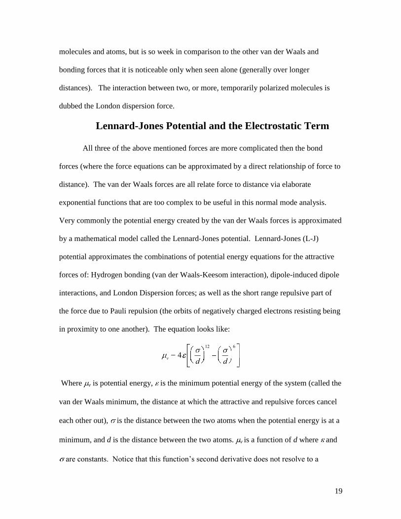
in proximity to one another). The equation looks like:

v 4d

12

d

6

Where v is potential energy, is the minimum potential energy of the system (called the

van der Waals minimum, the distance at which the attractive and repulsive forces cancel

each other out), is the distance between the two atoms when the potential energy is at a

minimum, and d is the distance between the two atoms. v is a function of d where and

are constants. Notice that this function‟s second derivative does not resolve to a

20

constant, k, like the various spring approximations did. At distances very close to the

minimized state the equation for L-J potential is sometimes approximated by a quadratic

(that does resolve to a constant) equation—In our program the entire second derivative is

used in the Hessian matrix.

The final component in the term, k ij , is derived by treating each atom as a simple

point charge. If the whole atom is regarded as one ball that has a net charge of q, then the

force between two atoms is given by Coulomb‟s Law:

Fq1q2

4 0d2

where q1 and q2 are the net charges, 0 is the electric permittivity of free space, and d is

the distance between the two atoms. The potential energy utilized by the two atoms in

proximity to one another is the integral of the force equation with respect to d. The

potential energy is called Coulomb potential and the equation describing it, “the

electrostatic term.”

c

q1q2

4 0d

The Final Form of “k”

Now the final meaning of the entries, k ij , in the Hessian matrix is apparent. The

values for kij are the sum, in component form, of all the second derivatives of potential

energy equations. Though the true physical processes are even more complex, this

equation is what the program we are using, parameters set AMBER99, uses to compute

the Hessian Matrix. The net potential energy between a set of two atoms is the sum of all

21

the sources of potential energy: stretching bonds, bending angles, twisting structures, L-J

potential, and Coulomb potential (electrostatic term):

net

1

2k (d d0 )2 k ( 0 )2 1

2k ( 0 )2 4

d

12

d

6qiq j

4 0d

Then the angles are rewritten using trigonometric functions to put them in terms of d.

The k function is then the second derivative of potential energy with respect to distance

(or position).

k ij2

net

d2

Then the distances are written in terms of vector displacements ( s ), and broken down

into component form ( x, y, z ). Then they are substituted into the H matrix. The

result is the Hessian matrix and the normal mode analysis equation. The parameters set

AMBER99 (or Assisted Model Building and Energy Refinement, 1999) provides all

necessary values for constants for any chemical bond or other force acting.

When this system of equations is solved to produce the eigenvalues and

eigenvectors we get the fundamental frequencies of the molecule. There are a total of

3n 6 frequencies for any non-linear molecule (six of the frequencies produced cause the

center of mass to move and are thus not valid for our purpose). In the case of the prion

E200K, 1734 atoms, this produces 5196 frequencies. Of these frequencies we then pick

one of the lowest frequencies for use in normal mode for excitation. Generally the lower

frequencies allow for greater displacements of large sections of the molecule while

smaller scale structures remain mostly intact and individual atoms do not move around as

much. There is a program in the molecular dynamics package, TINKER, that selects the

22

most efficient frequency based on desired displacements. Once the frequency is chosen

we use it to produce movement in the molecule through the property of resonance.

Resonance and Problems With the Model

Resonance is quite well known in its mechanical sense; a sound wave from one

tuning fork will cause a second tuning fork of the same fundamental frequency to vibrate.

Resonance, the idea that an object vibrating at its natural frequency will force another

object of the same natural frequency to vibrate, works not only with sound waves, but

with all kinds of waves—including electromagnetic waves. If the E200K protein is

bombarded with electromagnetic waves that are very close to one of its normal modes it

will be forced to vibrate at that frequency and thus its atoms will move in accordance

with the displacement vectors associated with that frequency. The frequency of the EM

wave we are hitting the modeled protein with is in the range of microwaves. If we

introduce enough energy into the prion quickly enough the amplitude of vibration will be

great; actually causing the molecule to refold in a different structure with a different

minimized state. If enough movement of large structures in the prion is achieved then the

imaginary springs connecting the atoms are stretched out enough so that they will reform

in a different configuration. Then the excess energy will be re-radiated or lost to heat—

allowing the molecule to stay in this new arrangement. This could potentially change the

structure of a damaging protein into something harmless by rearranging the positions of

the activation sites.

The main problems with this process are due to absorption, anharmonicity, and

instantaneous modes. If the calculated frequency is not close enough to the true

frequency, the molecule will not absorb the energy very well, and a much higher

23

amplitude (higher intensity) wave is required to excite the molecule. Any solvent

surrounding the molecule will also likely absorb a great deal of the energy before it

reaches the prion. Anharmonicity is a problem created by overtones. If you imagine a

guitar string, the string does not only vibrate at one frequency; its rich sound quality is

made up of multiple notes (frequencies) emanating from one vibration. The majority of

the vibration is at the fundamental frequency with decreasing amounts of vibrational

energy being transferred into integer multiples of that frequency. If this happens in the

molecular vibration it can disrupt the movement of the atoms. We get around this

problem by not allowing the molecule to vibrate for very long, we use one burst of

radiation for an extremely short period of time—so anharmonicity does not develop. The

final problem comes down to flaws in approximation. The normal mode frequencies are

only valid fundamental frequencies when the molecule is in, or very close to, its

minimized state; as soon as the molecule starts to move the frequencies change to

something called an instantaneous mode. The instantaneous mode is the fundamental

frequency in a non-minimized state, using more accurate models and factoring in the

kinetic energy of the moving atoms. This requires use of a G-Matrix rather the F-Matrix,

a much more complicated problem. We, again, are working around this problem by

applying all the energy to the prion very quickly, before it can move enough to

significantly change the fundamental frequency and reduce the absorption of the EM

waves.

The Carbon Dioxide Example

The last part of this section, devoted to background research and theoretical

understanding, gives an example of the process involved in finding normal modes with a

24

much-simplified model of a carbon dioxide atom. If we focus only on the stretch of the

bonds in one direction (the x component) and use only the simple spring approximation

(ignoring Lennard-Jones Potential and Coulomb forces) it greatly reduces the complexity

of the problem. The carbon dioxide molecule is linear, an oxygen double bonded to a

carbon in the center with another oxygen on the opposite side. Atom 1 is the left hand

oxygen, atom 2 is the center carbon, and atom 3 is the right hand oxygen. The mass

weighted Hessian matrix for this problem is:

kxx11

m1 m1

kxx12

m1 m2

kxx13

m1 m3

kxx21

m2 m1

kxx22

m2 m2

kxx23

m2 m3

kxx31

m3 m2

kxx32

m3 m2

kxx33

m3 m3

x1

x2

x3

4 2v2

x1

x2

x3

Next we use Newton‟s third law of motion to equate some of the terms; this is not often

possible due to the complexity of the L-J potential and electrostatic term. kxx12 kxx

21 and

kxx32 kxx

23 because of Newton‟s third law of motion. We assume kxx13 kxx

31 0 because

they are not directly bonded together and the non-bonded interaction forces are not

considered. The masses of each atom are inserted, in atomic mass units (carbon is 12amu

and oxygen is 16amu). Finally the values of k are inserted. Because kxx12 is attached to kxx

11

by a bond, the spring constant between the two is the same, but the direction opposite so

kxx11 kxx

12 . The same logic can be applied to kxx11 and kxx

21 as well as kxx33 : kxx

23 and kxx33 kxx

32 .

The approximate force constant for kxx11 is picked to be 1600Nm

-1, which, because of

symmetry is assumed to be the same as kxx33 (they are both double bonds between oxygen

and carbon). kxx22 is approximately 3200Nm

-1. Applying the above identities produces:

25

160016 16

160016 12

0

160012 16

320012 12

160012 16

0 160016 12

160016 16

x1

x2

x3

4 2v2

x1

x2

x3

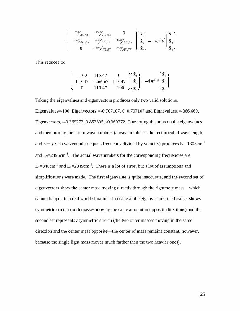
This reduces to:

100 115.47 0

115.47 266.67 115.47

0 115.47 100

x1

x2

x3

4 2v2

x1

x2

x3

Taking the eigenvalues and eigenvectors produces only two valid solutions.

Eigenvalue1=-100, Eigenvectors1=-0.707107, 0, 0.707107 and Eignevalues2=-366.669,

Eigenvectors2=-0.369272, 0.852805, -0.369272. Converting the units on the eigenvalues

and then turning them into wavenumbers (a wavenumber is the reciprocal of wavelength,

and v f so wavenumber equals frequency divided by velocity) produces E1=1303cm-1

and E2=2495cm-1

. The actual wavenumbers for the corresponding frequencies are

E1=340cm-1

and E2=2349cm-1

. There is a lot of error, but a lot of assumptions and

simplifications were made. The first eigenvalue is quite inaccurate, and the second set of

eigenvectors show the center mass moving directly through the rightmost mass—which

cannot happen in a real world situation. Looking at the eigenvectors, the first set shows

symmetric stretch (both masses moving the same amount in opposite directions) and the

second set represents asymmetric stretch (the two outer masses moving in the same

direction and the center mass opposite—the center of mass remains constant, however,

because the single light mass moves much farther then the two heavier ones).

26

The Computer Model: Tinker Tinker is both a molecular dynamics and molecular mechanics modeling

packages. This package uses the 1999 version of amber force constants to model the

interactions between atoms.

We felt it to be an ideal choice because it is open source and written in Fortran, a

language well suited for large mathematical models that we are capable of understanding

and modifying. Most importantly, however, it contained necessary programs that could

run that could run the necessary functions required for our project.

Program Flow The project may be broken down into many components. First we obtained the

structural data for the E200K variant Prion through the protein data bank which contains

data, obtained through x-ray crystallography in addition to other methods, on may

different proteins. After obtaining the structural data we minimized the protein for reason

described early. Next we ran the tinker program vibrate.x, which we slightly modified so

it would automatically print all the vibrational modes of the molecule. Next we ran our

program MDCompare which evaluated the modes and ranked them in order of interest to

our goal of deforming the Prion. Next, we ran another of our programs to set up a file to

run a Microcanonical Ensemble simulation that modeled the trajectories of the atoms

assuming that the Prion was activated with a specific frequency of electromagnetic

radiation and absorbed a certain amount of energy.

27

Minimizing the Protein Tinker‟s program to find the vibrational modes of a molecule is limited to

molecules in a minimized state where the molecule‟s potential energy exists in a local

minima meaning that if the molecule was slightly perturbed in any fashion it would gain

potential energy. Although the theory behind calculating fundamental frequencies or

normal modes of molecules that are not minimized and that have kinetic energy, an

implementation of this algorithm is unknown to our team and the complexity of the

theory and time needed to incorporate such a model made this expansion unfeasible for

our team.

For the simulations run inside of a vacuum this is a good approximation for what

the structure would look like were it inside of a vacuum. In addition, the original protein

structure we received from the protein data bank had been minimized according to their

force field. Since the exact nature of intermolecular force fields remains unknown to the

28

scientific community, there are many different programs that approximate intermolecular

forces and they all are slightly different.

However, for the simulations inside of a water box, which more closely resembles

a blood sample, this method fails to take into account the change in structure induced by

the water as well as the increase in kinetic energy due to the ambient heat of the blood.

Thus, if this method was to be considered for application, a more accurate method of

finding the vibrational modes is suggested.

Finding Ideal Vibrational Modes

In choosing vibrational modes to activate we felt that it would be most effective to

find the ones that appeared they would most effectively change the conditions we

consider in the analysis of the final, modified, Prion. Thus, we searched for Modes that

most effectively change the electrostatic surface potential and that would specifically

target our two identified activation sites where it is believed the E200K Prion attaches

onto other in order to get the host to conform to its structure and become a pathogenic

Prion.

In considering which modes would change the electrostatic surface potential the

most we determined that a change in atomic structure of the Prion would directly equate

to a change in the surface potential. In addition we found that water, which is a major

component of blood, absorbs less energy near the visible spectrum. We believe that the

more energy the Prion absorbs the more it will deform; thus a high frequency mode that

is close to the visible region is the ideal choice for this criterion.

In addition we specifically observed the activation sites of the Prion which were

located at atoms 697-769 and 1138-1207. We found modes where all or most of the

29

absorbed energy translated into the movement of these groups of atoms. In quantifying

this displacement we used the composite of the Mean Square Displacement Theorem one

each site.

We found these two selection criterion to be complementary to each other.

Absorption in the form of molecular vibrations generally occurs with wavelength smaller

than that of Infra-red radiation. In addition normal modes that are localized to particular

regions tend to be higher frequency where as the lower frequency modes create more

global movements of the atoms in the protein. Thus the criteria we observed lead us to

choose a higher frequency vibration mode.

Prion Vacuum Simulation

The fist series of trials deforming the E200k variant of the human Prion are

conducted in a vacuum. These simulations involved the activation of normal modes of the

Prion assuming 0 to ____ J of energy is absorbed from an electromagnetic wave. This

instantaneous mode activation is translated into velocities of each atom in the Prion.

This data is inserted into the molecular dynamics Microcanonical(NVE)

ensemble simulation included with the Tinker molecular modeling package. This

computer model determines the trajectories of each atom while conserving the amount of

atoms, volume in which they are contained, and the energy of the system. They are run

for a period 20 picoseconds with a time step of 1 femtosecond, which is the default for

tinker. It was observed that after 10ps many of the proteins in the NVE simulation

2)0()( rtrMSD

30

stopped deforming thus it was decided that a run length of 20 ps would allow sufficient

time for the Prion to reach a different local minima.

The scope of the project is to render inert the E200k mutant Prion in blood

donations, which makes this simulation inside of a vacuum unrealistic. By failing to take

into account a solvent, the ability to deform is greatly increased because as the atoms of

the Prion move, they do not interact with other molecules in the environment.

Prion Water Box Simulation

Water is chosen as a solvent to submerse the Prion for the molecular dynamic

simulations because it accounts for about 83% of human blood. In addition, the

polarization of water is related to the protein folding in such a way that the hydrophilic

parts align themselves towered the exterior while the hydrophobic portions dwell in the

interior of the Prion protein.

This simulation consisted of a hybrid of both the Microcanonical ensemble and

canonical ensemble. We recognized that blood samples are not stored at absolute zero, so

we assumed a temperature 298k for the blood samples to be stored at. After heating up

the water along with the protein a vibrational mode for each simulation was activated in a

Microcanonical ensemble, which conserves energy as compared to temperature. We

believe that during the activation of the normal mode, energy conservation is more

important because the electromagnetic wave is providing energy that will heat up a

sample of blood making temperature no longer a conserved quantity.

The tinker molecular modeling package did not come well suited for the creation

and use of a water solvent. Initially the water type hydrogen of the 1999 version of amber

parameters lacked a Van-Der-Waals radius causing any simulation involving water

31

molecules to become unstable and crash due to the occurrence of infinite energies created

by the hydrogen atoms overlapping other atoms. Thus, we decided to create insert our

own parameters into the 1999 amber parameter set. We used structural data of the water

molecule from London South Bank University. Additionally, we used force constants

from the CHARMM force field parameter set. This information allowed for the

formulation of a fairly stable water box.

The water box is created using the molecular mass and specific gravity. It is found

that the specific gravity of water is 995.65 Kg/m3

at around 300 degrees Kelvin. Thus:

Then by using the molecular mass of water, 18.01508, the number of molecules per gram

is found:

Knowing these two values it is then possible to determine the number of molecules per

Angstrom cubed in a sample of water:

This information may then be used in a computer model to create a box of water to

submerse the Prion protein.

The water box used in the simulations has sides of 40 angstroms. Using the

xyzedit tool from tinker the E200K mutant Prion is submersed into the water. Initially it

was believed that the 40 angstrom cube would be small enough to keep a relatively short

runtime while large enough to completely submerse the protein. However, later

observations proved that the cube was not large enough to house the protein which

32

caused an increase of the box size and the dispersion of the water molecules during the

simulation as shown in the visual representations below.

Figure 1 before Activation of Normal Mode. Notice the Prion, the blue and turquoise atoms, is not completely contained within the red and white water molecules

Figure 2 After a NVE simulation of a activated mode

33

Although the box stayed fairly together the results obtained uncountable are

affected by the error. Obviously the portions outside of the smaller box are freer to move

and reach different local minima than that of the initial. In addition, the ability of the

water molecules to escape resulted in a decrease in density of the water molecules around

the Prion thus allowing the entire Prion to deform more easily.

A larger water box that has sides 75 angstroms in length has already been initially

developed. However, due to the addition of new atoms the preparation time has increased

substantially, which has been compounded by the limitation that the minimization

program provided by tinker is not parallelized, limiting the preparation to a single

processor. In addition, the larger water box contains ten times as many atoms as the

original did so the model runtime which was already at twelve hours using 32 processors

is expected to dramatically increase.

Analysis Methods

Although we may only discover if a Prion has been sufficiently deformed to be

rendered inert through testing, there are physical aspects that may be observed to

hypothesize if it is still functional. It is believed that the loops consisting of residues 697

through 769 and 1138 through 1207 are key activation sites that enable the Prion to latch

on to other health and convert them to the pathogenic form of the Prion. In addition, it is

believed that the electrostatic surface potential also plays a vital role in the ability of the

E200K mutant Prion to make other conform to the unhealthy state.

To evaluate the effectiveness of the deformation based on these observations we

used the Mean Square Displacement Theorem:

34

We evaluated the function for three intervals: Once for each of the two loops and once

over the entire protein since electrostatic surface potential is the direct result of the

positioning of the atoms of the protein.

Results

From our current data it appears as if the lower frequency modes which result in

more global deformations of the Prion deformed the entire Prion and the loop regions

more than the mode that specifically targeted the loop region. In additon, the simulations

of the Prion in the vacume seem to reflect the results of the simulations in the water box

except in a much more exagerated manner.

Frequency 0.11cm-1

in Vacume

Figure 3: Series1 - Full protein Mean Square Displacement; Series 2 - First Loop Mean Square Displacement; Series3 - Second Loop Mean Square Displacement

2)0()( rtrMSD

35

Frequency 0.11cm-1

in Water Box

Figure 4: Series1 - Full protein Mean Square Displacement; Series 2 - First Loop Mean Square Displacement; Series3 - Second Loop Mean Square Displacement

Frequency 2999cm-1

in Vacume

Figure 5: Series1 - Full protein Mean Square Displacement; Series 2 - First Loop Mean Square Displacement; Series3 - Second Loop Mean Square Displacement

36

Frequency 2999cm-1

in Water Box

Figure 6: Series1 - Full protein Mean Square Displacement; Series 2 - First Loop Mean Square Displacement; Series3 - Second Loop Mean Square Displacement

Conclusion

We demonstrated that in a vacuum it is possible to significantly deform the Prion

to the point where we can consider it probably inert. However, when applying the same

method to the protein in the water box much more energy is needed to create the same

deformation in the Prion. In addition, the water box we built in tinker still had issues with

stability that prevented us from exploring activating these modes with the higher amounts

of energy needed. Consequently, as a future expansion, it would be beneficial if we used

a different molecular modeling package better suited for modeling water.

37

Thanks! We all send our thanks to Mr. McBeth for sponsoring us and making this all happen and

to Mark Fleharty, an excellent mentor who helped us through some difficult science,

math, and programming. Also, to all those who work behind the scenes to make the NM

Supercomputing Challenge happen—it has been a phenomenal experience!

Bibliography Hirst Group Homepage. 25 Feb. 2009

<http://comp.chem.nottingham.ac.uk/teaching/F14CCH/charmmtutorial.pdf>.

"Water molecule structure." London South Bank University - become what you want to

be. 25 Feb. 2009 <http://www.lsbu.ac.uk/water/molecule.html>.

Wilson, E. Bright, J. C. Decius, and P. C. Cross. Molecular Vibrations : The Theory of

Infrared and Raman Vibrational Spectra. Minneapolis: Dover Publications,

Incorporated, 1980

"RCSB PDB : Structure Explorer." 27 Feb. 2009

<http://www.pdb.org/pdb/explore/explore.do?structureId=1FKC>.

Prusiner, Stanley B. Prion biology and diseases. Cold Spring Harbor, N.Y: Cold Spring

Harbor Laboratory P, 2004.

"TINKER Molecular Modeling Package." Jay Ponder Lab Home Page. 27 Feb. 2009

<http://dasher.wustl.edu/tinker/>.

“Hydrogen Bond-Wikipedia” Wikipedia 30 March 2009

<http://en.wikipedia.org/wiki/Hydrogen_Bond>

“Explain van der Waals Forces to me” PHYSLINK.COM 25 March 2009

<http://www.physlink.com/Education/AskExperts?ae206.cfm

“Potential Well” Wikipedia 24 March 2009

<http://en.wikipedia.org/wiki/Potential_well>

“Lennard-Jones potential” Wikipedia 25 March 2009

<http://en.wikipedia.org/wiki/Lennard_Jones_Potential>

“van der Waals force” Wikipedia 27 March 2009

<http://en.wikipedia.org/wiki/Van_der_Waals_forces>

Kolman, Bernard Introductory Linear Algebra With Applications Macmillan Publishing

Company: New York, New York. 1984

“Torsion Spring” Wikipedia 25 March 2009

<http://en.wikipedia.org/wiki/Torsion_spring>

“Hessian Matrix” Wikipedia 19 Febuary 2009

<http://en.wikipedia.org/wiki/Hessian_matrix>

38

Parallelized Code #include <cstdlib> #include "mpi.h" #include <iostream> #include <sstream> #include <string> using namespace std; int main(int argc, char *argv[]) { string baseName = "1FKCWM"; //numprocs - number of processors //mynum - current processor's number int numprocs, mynum; //prepare comunication between nodes MPI_Init(&argc, &argv); //get the number of processors MPI_Comm_size(MPI_COMM_WORLD, &numprocs); //get processor number MPI_Comm_rank(MPI_COMM_WORLD, &mynum); float start = atof(argv[1]); float end = atof(argv[2]); float res = atof(argv[3]); int size = ( end - start ) / res; //number of simulations for each precessor.... +1 is to make sure program does more runs if sze/numprocs != whole # int blkSize = size / numprocs + 1; //create Dyn Files stringstream command; command << "./mode 1FKC.xyz vibrate.log " << blkSize * mynum * res + start << " " << blkSize * ( mynum + 1 ) * res + start << " " << res; system(command.str().c_str()); //runDynamic for ( int i = 0; i < blkSize; i++ ) { float curAmp = start + (float)mynum * blkSize * res + (float)i * res;

39

//set Files for dynamic stringstream command2; command2 << "cp " << baseName << ".xyz " << baseName << "_" << curAmp << ".xyz"; system(command2.str().c_str()); //run Dynamic stringstream command3; command3 << "/users/jfenc/tinker/bin/dynamic.x " << baseName << "_" << curAmp << " 20000 1 .1 1"; system(command3.str().c_str()); //clean up stringstream command4; command4 << "cat " << baseName << "_" << curAmp << ".[0-9][0-9][0-9] > " << baseName << "_" << curAmp << ".arc"; system(command4.str().c_str()); stringstream command5; command5 << "cp " << baseName << "_" << curAmp << ".200 ../data"; system(command5.str().c_str()); stringstream command6; command6 << "cp " << baseName << "_" << curAmp << ".arc ../data"; system(command6.str().c_str()); stringsream command7; command7 << "mkdir " << curAmp; system(command7.str()); stringstream command8; command8 << "mv " << baseName << "_" << curAmp << "* " << curAmp; system(command8.str()); } //close all connecntions MPI_Finalize(); system("PAUSE"); return EXIT_SUCCESS; }

40

Dynamic File Creator /****************************************************** //Title: DYNMAKE // //Description: Create dynamic Files for a NVE simulation // // //Arguments: 1) Log File Name // 2) XYZ File // 3) Start // 4) End // 5) Resolution // 6) Mode *******************************************************/ #include <cstdlib> #include <iostream> #include <string> #include <sstream> #include <vector> #include <fstream> #include "VibrateMode.h" #include "AtomSet.h" using namespace std; int main(int argc, char *argv[]) { float start = atof(argv[3]); float stop = atof(argv[4]); float res = atof(argv[5]); int mode = atoi(argv[6]); string fName = argv[1]; string log = argv[2];

41

AtomSet set(fName); set.GetD_(log, mode); for ( float i = start; i < stop; i += res ) { ofstream dyn; dyn.open ( "i" ); stringstream name; name << "data/" << mode << "_" << i; set.writeDyns( name.str(), i ); } system("PAUSE"); return EXIT_SUCCESS; }

Table Creator /****************************************************** //Title: Table // //Description: Reads the output of the NVE water Box simulations and creates a graph // a graph showing MSD of selected atoms // //Arguments: 1) XYZ Original File 2) baseName // 3) start // 4) stop *******************************************************/ #include <cstdlib> #include <iostream> #include <string> #include <sstream> #include <vector> #include <fstream> #include "VibrateMode.h" #include "AtomSet.h" using namespace std; int main(int argc, char *argv[]) { float start = 0; float stop = 1000; float res = 10; int mode = 4881; string baseName = "1FKCWM"; string original = "1FKC.xyz"; string vibratelog = "vibrate.log"; ofstream table;

42

table.open ( "MSDTable" ); for ( float i = start; i < stop; i += res ) { stringstream file; file << baseName << "_" << i << ".200"; //check to see if file is there ifstream tFile; tFile.open( file.str().c_str() ); if ( tFile ) { tFile.close(); AtomSet set(file.str()); AtomSet set2(file.str()); set2.ReadParam("SAmber"); set2.GetD_( vibratelog, mode ); set2.RemoveWater(); table << i << "\t" << set2.energy(i) << "\t" << set.MSD(original, 0, 1734) << "\t" << set.MSD(original, 697, 769) << "\t" << set.MSD(original, 1138, 1207) << endl; } } table.close(); system("PAUSE"); return EXIT_SUCCESS; }

43

Mode Comparison /****************************************************** //Title: MDCompare // //Description: Compares the different modes and creates // a graph showing MSD of selected atoms // //Arguments: 1) Log File Name 2) XYZ File // 3) Start Atom // 4) End Atom *******************************************************/ #include <cstdlib> #include <iostream> #include <string> #include <sstream> #include <vector> #include <fstream> #include "VibrateMode.h" #include "AtomSet.h" using namespace std; int main(int argc, char *argv[]) { if ( argc != 5 ) { cerr << "INCORRECT ARGS" << endl; exit(1); } stringstream temp; temp << argv[1]; string logFile; temp >> logFile; stringstream temp1; temp1 << argv[2]; string xyzFile; temp1 >> xyzFile; stringstream temp2; temp2 << argv[3];

44

int start; temp2 >> start; stringstream temp3; temp3 << argv[4]; int end = 1207; temp3 >> end; AtomSet::AtomSet protein( xyzFile ); int atCt = protein.count(); int fCt = 5201;//VibrateMode::ct( logFile, atCt); stringstream compName; compName << "mdComp_" << start << "_" << end << ".txt"; ofstream outdata; outdata.open( compName.str().c_str() ); if ( !outdata ) { cerr << "FAILED" << endl; } vector<float> total(5201); for ( int i = 1; i < fCt + 1; i++ ) { VibrateMode::VibrateMode mode( atCt, logFile, i ); float sec1 = mode.MSD( 697, 769 ); float sec2 = mode.MSD( 1138, 1207 ); total[i - 1] = sec1 + sec2; outdata << i << "\t" << sec1 << "\t" << sec2 << "\t" << mode.getF() << endl; } ofstream top; top.open("top.txt"); for ( int i = 0; i < 15; i++ ) { int topLoc = 0; for ( int j = 0; j < fCt; j++ ) { if ( total[j] > total[topLoc] ) topLoc = j; top << topLoc + 1 << "\t" << total[topLoc] << endl; } } top.close(); system("PAUSE"); return EXIT_SUCCESS; }

45

AtomSet.h #ifndef ATOMSET_H #define ATOMSET_H #include <iostream> #include <fstream> #include <vector> #include <string> #include <cstdlib> #include <cmath> #include <sstream> #include "DataStructures.h" #include "VibrateMode.h" using namespace std; class AtomSet { private: vector<Atom> *atoms; vector<float> *f; vector<float> *m; int atCt; public: AtomSet( string xyzFile ); ~AtomSet(); void GetD_( string vibFile, int mode ); void writeArc( string arcFile, int res ); void writeDyns( string dynFile, float mag); void ToPDB( string PDBFile, string name ); float MSD( string xyzOriginal, int start, int stop ); float energy( float Amplitude ); void ReadParam(string SAParam ); void RemoveWater(); float GetF(); int count(); private: void GetP_( string xyzFile ); string fileLine( float x, float y, float z, Atom atom, int number ); string cordIntro( int atomCt, string name ); float getPosition( float cord, float totalChange, float t ); float mag( Point p1, Point p2 ); };

46

#endif

AtomSet.cpp #include "AtomSet.h" #define MAXBONDS 5 #define ATOMDIGITS 4 #define PI 3.14159265 using namespace std; AtomSet::AtomSet( string xyzFile ) { atoms = new vector<Atom>(0); f = new vector<float>(0); GetP_( xyzFile ); }; AtomSet::~AtomSet() { delete atoms; delete f; }; void AtomSet::GetP_( string xyzFile ) { ifstream indata; indata.open( xyzFile.c_str() ); if ( !indata ) { cout << "FAILED" << endl; } indata >> atCt; //skip line char line[256]; indata.getline(line, 256); for ( int i = 0; i < atCt; i++ ) { int linenum = 0; indata >> linenum; Atom na; //indata.getline(line, 256); indata >> na.name; indata >> na.p_.x; indata >> na.p_.y;

47

indata >> na.p_.z; atoms->push_back(na); indata.getline(line, 256); stringstream ln(stringstream::in | stringstream::out); ln << line; for ( int j = 0; j < MAXBONDS; j++ ) ln >> (*atoms)[ i ].bonds[ j ]; } }; void AtomSet::GetD_( string fileName, int modenum ) { VibrateMode mode(atCt, fileName, modenum); (*f)[ 0 ] = mode.getF(); for ( int i = 0; i < atCt; i++ ) (*atoms)[ i ].d_ = (*mode.d_)[ i ]; }; void AtomSet::writeArc(string arcFile, int res ) { int c = f->size(); int p = atoms->size(); ofstream arc; stringstream file; file << arcFile << "_" << (*f)[0] << ".arc"; arc.open (file.str().c_str()); for ( int j = 0; j < res; j++ ) { arc << cordIntro(atCt, arcFile) << endl; for ( int k = 0; k < atCt; k++ ) { float x = getPosition( (*atoms)[ k ].p_.x, (*atoms)[ k ].d_.x, 2 * PI * (float)j / (float)res ); float y = getPosition( (*atoms)[ k ].p_.y, (*atoms)[ k ].d_.y, 2 * PI * (float)j / (float)res ); float z = getPosition( (*atoms)[ k ].p_.z, (*atoms)[ k ].d_.z, 2 * PI * (float)j / (float)res ); arc << fileLine(x, y, z, (*atoms)[ k ], k + 1 ) << endl; if ( k > 0 ) int x = 3; } } arc.close(); }; void AtomSet::ToPDB ( string PDBFile, string name ) { ifstream indata; indata.open( PDBFile.c_str() ); if ( !indata ) { cerr << "FAILED" << endl; } ofstream outdata; outdata.open( name.c_str() ); if ( !outdata ) { cerr << "FAILED" << endl; } bool isText = true; while ( isText ) { isText = false; char line[256]; indata.getline(line, 256); stringstream lstream; lstream << line; string fword; lstream >> fword;

48

if ( fword.length() > 0 ) isText = true; int atNum = 0; if ( fword == "ATOM" ) { stringstream nLine; nLine << "Atom \t"; for ( int i = 0; i < 5; i++ ) { string word; lstream >> word; nLine << word << "\t"; } nLine << (*atoms)[ atNum ].p_.x << "\t"; nLine << (*atoms)[ atNum ].p_.y << "\t"; nLine << (*atoms)[ atNum ].p_.z << "\t"; for ( int i = 0; i < 3; i++ ) { string word; lstream >> word; nLine << word << "\t"; } atNum++; } else outdata << line; } } float AtomSet::GetF() { return (*f)[ 0 ]; } int AtomSet::count() { return atCt; } string AtomSet::cordIntro( int atomCt, string name ) { stringstream ln(stringstream::in | stringstream::out); ln << " " << atomCt << " " << name ; return ln.str(); }; string AtomSet::fileLine( float x, float y, float z, Atom atom, int number ) { stringstream ln(stringstream::in | stringstream::out); ln << " " << number << " " << atom.name << " " << x << " " << y \ << " " << z << " "; for ( int i = 0; i < MAXBONDS; i++ ) { ln << " "; ln << atom.bonds[i]; } return ln.str(); }; float AtomSet::getPosition( float cord, float totalChange, float t) { return 3 * totalChange * sin(t) + cord; };

49

void AtomSet::writeDyns(string dynFile, float mag) { cout << "writeing dns" << endl; ofstream dyn; dyn.open ( dynFile.c_str() ); dyn << "Number of Atoms and Title :" << endl; dyn << " " << atoms->size() << " " << dynFile << endl; dyn << "Periodic Box Dimensions :" << endl; dyn << " " << "90" << " " << "90" << " " << "90" << endl; dyn << " " << "90" << " " << "90" << " " << "90" << endl; dyn << "Current Atomic Positions : " << endl; for ( int j = 0; j < atoms->size(); j++ ) { dyn << " " << (*atoms)[ j ].p_.x << " " << (*atoms)[ j ].p_.y << " " << (*atoms)[ j ].p_.z << endl; } dyn << "Current Atomic Velocities :" << endl; for ( int j = 0; j < atoms->size(); j++ ) { dyn << " " << mag * (*atoms)[j].d_.x << " " << mag * (*atoms)[j].d_.y << " " << mag * (*atoms)[j].d_.z << endl; } dyn << "Current Atomic Accelerations :" << endl; for ( int j = 0; j < atoms->size(); j++ ) { dyn << " " << 0 << " " << 0 << " " << 0 << endl; } dyn << "Previous Atomic Accelerations :" << endl; for ( int j = 0; j < atoms->size(); j++ ) { dyn << " " << 0 << " " << 0 << " " << 0 << endl; } dyn.close(); }; float AtomSet::MSD(string originalFile, int start, int stop) { AtomSet orig(originalFile); float sum = 0; for ( int i = start; i < stop; i++ ) { sum += sqrt(pow((*atoms)[i].p_.x - (*orig.atoms)[i].p_.x,2)+pow((*atoms)[i].p_.y - (*orig.atoms)[i].p_.y,2)+pow((*atoms)[i].p_.z - (*orig.atoms)[i].p_.z,2)); } sum /= stop - start; return sum; }; float AtomSet::energy( float Amplitude) { //1/2MV^2 on each atom double E = 0; for ( int i = 0; i < atCt; i++ ) { Point z; z.x = 0; z.y = 0; z.z = 0; float v = Amplitude * mag((*atoms)[i].d_, z) * 100; float mass = (*m)[ atoi((*atoms)[ i ].bonds[ 0 ].c_str()) - 1]; // KE = 1/2mv^2; u -> kg; angstroms/picosecond -> meters/sec; J -> eV E += mass * pow(v, 2) / 2 * 1.66053 * 6.2415 * 1e-9; } cout << E << endl; return E;

50

} //gets the mass of all atoms as identified by their number which is the location in the array + 1 void AtomSet::ReadParam ( string SAParam ) { m = new vector<float>(1252); ifstream indata; indata.open( SAParam.c_str() ); if ( !indata ) { cout << "FAILED" << endl; } for ( int i = 0; i < 1252; i++ ) { indata >> (*m)[i]; } } void AtomSet::RemoveWater() { vector<Atom> newSet(0); for ( int i = 0; i < atCt; i++ ) { int ID = atoi((*atoms)[ i ].bonds[ 0 ].c_str()); if ( ID > 1254 ) { atoms->erase(atoms->begin() + i); atCt--; i--; } } } float AtomSet::mag( Point p1, Point p2 ) { return sqrt(pow(p1.x - p2.x,2)+pow(p1.y - p2.y,2)+pow(p1.z - p2.x,2)); };

51

‘

VibrateMode.h

#ifndef VIBRATEMODE_H #define VIBRATEMODE_H #include <iostream> #include <fstream> #include <vector> #include <string> #include <sstream> #include <cstdlib> #include <cmath> #include <sstream> #include "DataStructures.h" using namespace std; class VibrateMode { friend class AtomSet; private: vector<Point> *d_; float f; string logFile; int *atCt; public: VibrateMode( int atCt, string logFile, int mode ); ~VibrateMode(); float MSD( int first, int last); static int ct( string log, int atomCt ); float getF(); void print(); private: void ReadMode( int mode ); void ReadLine( float *x, float *y, float *z, ifstream& file ); void GoToMode( ifstream& fileStrm ); static void SkipLines( ifstream& fileStrm, int lines ); float mag( Point p1 ); }; #endif

52

VibrateMode.cpp #include "VibrateMode.h" using namespace std; VibrateMode::VibrateMode ( int atCt, string logFile, int mode ) { d_ = new vector<Point>(0); int temp = atCt; this->atCt = new int(temp); // memory stompping issues this->logFile = logFile; ReadMode ( mode ); }; VibrateMode::~VibrateMode() { delete d_; }; void VibrateMode::ReadMode ( int mode ) { //Open File ifstream indata; indata.open(logFile.c_str()); if (!indata) { cout << "FAILED" << endl; } GoToMode(indata); string modeHdr = "Vibrational Normal Mode"; bool isMode = true; d_->resize( *atCt ); int fCt = 0; while( isMode ) //Read Displacements { //seek down 2 lines char modeHeader [ 256 ]; indata.getline(modeHeader, 256); string hdr = modeHeader; if ( hdr != "" ) { if ( 0 == modeHdr.compare( hdr.substr(1,23) ) ) { isMode = true; SkipLines(indata, 3);

53

fCt++; cout << fCt << endl; if (fCt == mode ) { d_->resize( *atCt ); stringstream head; head << hdr; //seek to right word of title string fstr; for ( int i = 0; i < 7; i++ ) head >> fstr; f = atof(fstr.c_str()); //save data for ( int i = 0; i < *atCt; i++ ) ReadLine( &(*d_)[ i ].x, &(*d_)[ i ].y, &(*d_)[ i ].z, indata ); break; break; } else { isMode = true; } } } } indata.close(); }; float VibrateMode::MSD ( int first, int last ) { int temp = *atCt; float sum = 0; for ( int i = first; i < last + 1; i++ ) { sum += pow(mag((*d_)[i]), 2); } sum /= (float)*atCt; return sum; }; void VibrateMode::print() { for ( int i = 0; i < 1734; i++ ) cout << (*d_)[i].x << " " << (*d_)[i].y << " " << (*d_)[i].z << endl; } int VibrateMode::ct ( string log, int atomCt ) { //Open File ifstream indata; indata.open(log.c_str()); if (!indata) { cout << "FAILED" << endl; } int lines = 23 + ( 3 * atomCt / 5 ) * 2 ; SkipLines(indata, lines); string modeHdr = "Vibrational Normal Mode"; bool isMode = true; int fCt = 0; while( isMode ) //Read Displacements { isMode = false; //seek down 2 lines SkipLines(indata,1); char hdr [ 256 ];

54

indata.getline(hdr, 256); string hdrs = hdr; if ( 0 == modeHdr.compare( hdrs.substr(1,23) ) ) fCt++; } indata.close(); return fCt; } float VibrateMode::getF () { return f; } void VibrateMode::ReadLine ( float *x, float *y, float *z, ifstream& file ) { char line[256]; file.getline(line,256); stringstream ln; ln << line; int atom; ln >> atom; ln >> *x; ln >> *y; ln >> *z; }; //Go to first line of atom displacements void VibrateMode::GoToMode ( ifstream& fileStrm ) { int lines = 24 + ( 3 * *atCt / 5 ) * 2 ; SkipLines(fileStrm, lines); }; void VibrateMode::SkipLines ( ifstream& fileStrm, int lines ) { char line[256]; for ( int j = 0; j < lines; j++ ) fileStrm.getline(line,256); } float VibrateMode::mag(Point p1) { return sqrt(pow(p1.x, 2)+pow(p1.y, 2)+pow(p1.z, 2)); };

55

DataStructures.h

#ifndef DATASTRUCTURES_H #define DATASTRUCTURES_H #include <vector> #include <string> #define MAXBONDS 5 using namespace std; struct Point { float x; float y; float z; }; struct Atom { Point p_; Point d_; string name; string bonds[MAXBONDS]; }; #endif