Rev. Sci. Instrum. 90, 015112 (2019); https://doi.org/10.1063/1.5066618 90, 015112

© 2019 Author(s).

Vibration isolation with high thermalconductance for a cryogen-free dilutionrefrigerator

Cite as: Rev. Sci. Instrum. 90, 015112 (2019); https://doi.org/10.1063/1.5066618Submitted: 16 October 2018 . Accepted: 24 December 2018 . Published Online: 23 January 2019

Martin de Wit , Gesa Welker , Kier Heeck, Frank M. Buters, Hedwig J. Eerkens , Gert Koning,

Harmen van der Meer, Dirk Bouwmeester, and Tjerk H. Oosterkamp

COLLECTIONS

This paper was selected as an Editor’s Pick

Review ofScientific Instruments ARTICLE scitation.org/journal/rsi

Vibration isolation with high thermalconductance for a cryogen-freedilution refrigerator

Cite as: Rev. Sci. Instrum. 90, 015112 (2019); doi: 10.1063/1.5066618Submitted: 16 October 2018 • Accepted: 24 December 2018 •Published Online: 23 January 2019

Martin de Wit,1,a) Gesa Welker,1,a) Kier Heeck,1 Frank M. Buters,1 Hedwig J. Eerkens,1 Gert Koning,1

Harmen van der Meer,1 Dirk Bouwmeester,1,2 and Tjerk H. Oosterkamp1,b)

AFFILIATIONS1Leiden Institute of Physics, Leiden University, P.O. Box 9504, 2300 RA Leiden, The Netherlands2Department of Physics, University of California, Santa Barbara, California 93106, USA

a)Contributions: M. de Wit and G. Welker contributed equally to this work.b)Electronic mail: oosterkamp@physics.leidenuniv.nl

ABSTRACTWe present the design and implementation of a mechanical low-pass filter vibration isolation used to reduce the vibrationalnoise in a cryogen-free dilution refrigerator operated at 10 mK, intended for scanning probe techniques. We discuss the designguidelines necessary to meet the competing requirements of having a low mechanical stiffness in combination with a high ther-mal conductance. We demonstrate the effectiveness of our approach by measuring the vibrational noise levels of an ultrasoftmechanical resonator positioned above a superconducting quantum interference device. Starting from a cryostat base tempera-ture of 8 mK, the vibration isolation can be cooled to 10.5 mK, with a cooling power of 113 µW at 100 mK. We use the low vibrationsand low temperature to demonstrate an effective cantilever temperature of less than 20 mK. This results in a force sensitivity ofless than 500 zN/

√Hz and an integrated frequency noise as low as 0.4 mHz in a 1 Hz measurement bandwidth.

© 2019 Author(s). All article content, except where otherwise noted, is licensed under a Creative Commons Attribution (CC BY) license(http://creativecommons.org/licenses/by/4.0/). https://doi.org/10.1063/1.5066618

I. INTRODUCTIONIn recent years, there is ever increasing interest in

the ability to work at very low temperatures with min-imal mechanical noise. This is evidenced by the largenumber of low-temperature instruments developed forthis purpose in a variety of scanning probe techniques,such as Scanning Tunneling Microscopy (STM),1–12 AtomicForce Microscopy (AFM),13,14 Magnetic Resonance ForceMicroscopy (MRFM),15–17 and other scanning probe tech-niques.18–21 Other examples include instruments intended toinvestigate the quantum properties of macroscopic objectswhere resonators with extremely low mode temperatures arerequired.22,23 However, vibration-sensitive measurements atlow temperatures remain a technological challenge, one of thereasons being the added vibrational noise introduced by thecooling equipment.

The specific vibrational requirements vary depending onthe technique. STM and the related Scanning Tunneling Spec-troscopy (STS) are notoriously sensitive to changes in thetip-sample distance. The tunneling current is exponentiallydependent on this distance z,24 leading to a required stabil-ity below 1 pm within the bandwidth (BW) of the I/V converter(typically a few Hz to several kHz).6,7,9 For techniques like AFM,Magnetic Force Microscopy (MFM), and MRFM, the low fre-quency stability criteria are less strict, with δz ≤ 10 pm.13,14,25Additionally, these techniques also require low vibration levelsnear the resonance frequency of the cantilever (typically 1-100kHz). The upper limit on the allowed vibration noise aroundthe cantilever frequency can be derived from the thermal dis-placement noise. This depends on the cantilever’s propertiesand operating temperature. For our specific MRFM setup, weaim for vibrations near the resonance frequency on the order

Rev. Sci. Instrum. 90, 015112 (2019); doi: 10.1063/1.5066618 90, 015112-1

© Author(s) 2019

Review ofScientific Instruments ARTICLE scitation.org/journal/rsi

of tens of femtometers per unit bandwidth at a temperature of100 mK.

Global solutions that attenuate vibrations outside of thecryostat work very well for a wide variety of systems. Com-mon measures include, e.g., mounting of the cryostat on aheavy platform, placing pumps in separate rooms, or usingsand to dampen vibration transfer via vacuum lines.7–11 How-ever, a local solution within the cryostat may be requiredwhen, for instance, it is not possible to create a stiff mechani-cal loop between the tip and the sample or when the cryostatis based on a cryocooler, e.g., a pulsetube, in which case signif-icant vibrations are generated within the cryostat itself.26,27 Inthese cases, one has to solve the combined problem of obtain-ing a high thermal conductance with low vibration noise,which is generally considered hard to do.28,29 The reason forthis is that most vibration isolation systems are based on amechanical low-pass filter with a corner frequency well belowthe desired operating frequency of the instrument, whichmeans that the stiffness of the vibration isolation should below. However, the thermal conduction scales with the cross-sectional area of the thermal link and is therefore higher for astiff connection. These conflicting requirements for the stiff-ness of the vibration isolation often lead to a compromisefor one of the two properties.30–32 Here we present a designwhich optimizes both aspects.

The vibration isolation presented in this article isintended to be used for a low temperature MRFM setup, wherean ultrasoft resonator is used to measure the properties ofvarious spin systems.33 Due to the low stiffness and high qual-ity factor of the resonator, the system is extremely sensi-tive to small forces34 and therefore to vibrations. We explainthe correspondence between electrical and mechanical net-works, as this analogue proves to be very useful for calcu-lating the optimal design of our mechanical filter. The filterwe present here was designed to fit in an experimental spaceof 55 cm length and to carry a load of several kilograms. Itshould be effective in the frequency range starting from 50 Hzup to about 100 kHz. However, our general design princi-ples also allow us to build a filter with a different bandwidth,tailored to the frequency range needed in scanning probetechniques such as STM/STS and AFM or for experimentsworking towards macroscopic superpositions. We will demon-strate the effectiveness of the vibration isolation by analyzingthe displacement noise spectrum and thermal properties ofthe MRFM resonator, showing that our method has allowed usto successfully combine a high thermal conductance and lowmechanical vibrations.

II. FILTER DESIGNCommonly, the development of mechanical vibration iso-

lation relies heavily on finite element simulations to deter-mine the design parameters corresponding to the desiredfilter properties. In these simulations, the initial design istweaked until the desired filter properties are found. Instead,we determined the parameters of our mechanical filter byfirst designing an electrical filter with the desired properties

and then converting this to the mechanical equivalent usingthe current-force analogy between electrical and mechanicalnetworks. This allows us to precisely specify the desired fil-ter properties beforehand, from which we can then calculatethe required mechanical components. We therefore find theoptimal solution using analytical techniques rather than usingcomplex simulations. As we will see later, this also allows us touse our design principle across many frequency scales with-out requiring a new finite element analysis. The correspondingquantities for the analogy between electrical and mechani-cal circuits are found in Table I. We choose the current-forceanalogy over the voltage-force analogy35 because the formerconserves the topology of the network.

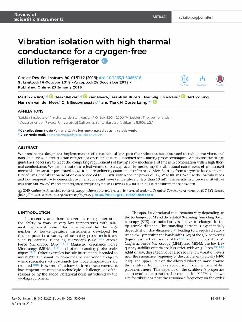
To design our desired filter, we follow the method ofCampbell for the design of LC wave-filters.36 Campbell’s filterdesign method is based on two requirements:

• The filter is thought to be composed out of an infiniterepetition of identical sections, as shown in Fig. 1(a),where a single section (also called unit cell) is indicatedby the black dotted box.

• The sections have to be dissipationless to preventsignal attenuation in the pass-band. Therefore theimpedances of all elements within the section have tobe imaginary.

Following these requirements, the edges of the transmit-ted frequency band of the filter are defined by the inequality

− 1 ≤Z1

4Z2≤ 0. (1)

The iterative impedance is the input impedance of a unitcell when loaded with this impedance. In order to preventreflections within the pass-band, the signal source and theload should have internal impedances equal to Ziter. The iter-ative impedance should be real and frequency-independentbecause this maximizes the power transfer within the pass-band and is easiest to realize.

There are three principle choices for the unit cell, all givenin Fig. 1(b). The total attenuation is determined by the num-ber of unit cells. Each unit cell acts like a second order fil-ter, adding an extra 40 dB per decade to the high frequencyasymptote of the transfer function. This attenuation is causedby reflection, not by dissipation, which is very important forlow-temperature applications.

TABLE I. Table of corresponding electrical and mechanical quantities.

Electrical Mechanical

Variable Symbol Variable Symbol

Current I (A) Force F (N)Voltage U (V) Velocity v (m/s)Impedance Z (Ω) Admittance Y (s/kg)Admittance Y (1/Ω) Impedance Z (kg/s)Resistance R (Ω) Responsiveness 1/D (s/kg)Inductance L (H) Elasticity 1/k (m/N)Capacitance C (F) Mass m (kg)

Rev. Sci. Instrum. 90, 015112 (2019); doi: 10.1063/1.5066618 90, 015112-2

© Author(s) 2019

Review ofScientific Instruments ARTICLE scitation.org/journal/rsi

FIG. 1. (a) General scheme of a filter composed of identical sections, with oneunit cell indicated by the black dotted box. (b) Three options for the design of theunit cell for an LC filter, with on the right the corresponding values for the iterativeimpedance Ziter .

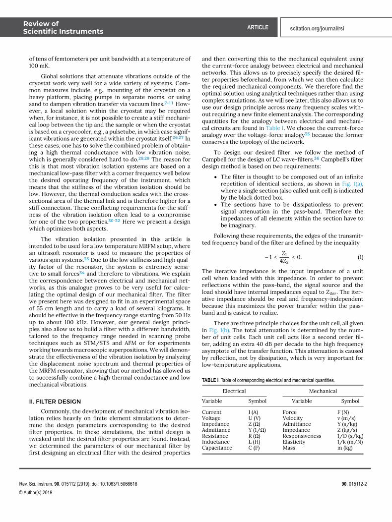
The design of the mechanical filter is straightforwardwhen we use the third option from Fig. 1(b) with Z1 =

1Y1= iωL

and Z2 =1Y2= 1

iωC . The resulting electrical low-pass filter isshown in Fig. 2(a). Note that the two neighboring 2Z2 in themiddle add up to Z2. We can use Eq. (1) to calculate the bandedges: ω1 = 0 and ω2 =

2√LC

.

With the electrical filter figured out, we make the trans-fer to the mechanical filter according to the correspondence,as outlined in Table I. As the electrical inductance correspondsto mechanical elasticity, the coils are replaced by mechanical

FIG. 2. (a) Electrical filter consisting of two unit cells. (b) Corresponding mechanicalfilter.

springs with stiffness k. The capacitors are replaced by massesin the mechanical filter. Note that the first mass has thevalue m

2 due to the specific unit cell design. The currentsource becomes a force source, and the electrical input andload admittances become mechanical loads (dampers). Thefinal mechanical circuit is depicted in Fig. 2(b). Going tothe mechanical picture also implies a conversion betweenimpedance and admittance in Eq. (1),

− 1 ≤Y1

4Y2≤ 0, (2)

with Y1 =kiω and Y2 = iωm, this leads to the band edges ω1 = 0

and ω2 = 2√

km , respectively.

We now have a design for the unit cell of a generalmechanical low-pass filter. The bandwidth and corner fre-quency are determined by the choice of the stiffness k andmass m, which can be tailored to the needs of a specific exper-imental setup. In practice, only corner frequencies between afew Hz and 50 kHz can be easily realized. At too low frequen-cies, the necessary soft springs will not be able to supportthe weight anymore, whereas above 50 kHz, the wavelengthof sound in metals comes into play, potentially leading to theexcitation of the eigenmodes of the masses.

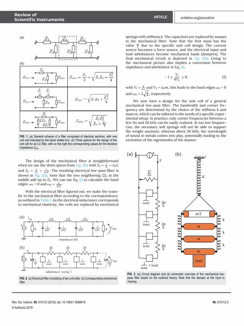
FIG. 3. (a) Circuit diagram and (b) schematic overview of the mechanical low-pass filter based on the outlined theory. Note that the damper at the input ismissing.

Rev. Sci. Instrum. 90, 015112 (2019); doi: 10.1063/1.5066618 90, 015112-3

© Author(s) 2019

Review ofScientific Instruments ARTICLE scitation.org/journal/rsi

A second practical challenge is the realization of thedamper at the end of the filter. It should be connected to themechanical ground, just as an electrical load is connected tothe electrical ground. This is, however, not possible becausethis mass reference point is defined by Earth’s gravity. Thealternative to a damper as a real-valued load is using a purelyreactive load: more mass. Simulations show that adding massto the m/2 of the filter’s last mass does not significantly alterthe frequency characteristics of the filter and even increasesthe attenuation. There is no strict limit on the weight of theadded mass. In fact, adding more will, in principle, improve thefilter. In practice, the limit depends on the choice of springs,which should be able to carry the weight whilst staying inthe linear regime. The downside of replacing the damper withmass is that we lose the suppression of the resonance fre-quencies of the filter. We have chosen a final mass with aweight equal to the previous mass. The circuit diagram andschematic for the final design of the mechanical low-pass fil-ter are shown in Fig. 3. Note that the damper at the input ismissing, for experimental reasons which will be explained inSec. IV B.

III. PRACTICAL DESIGN AND IMPLEMENTATIONOur setup is based on a Leiden Cryogenics CF-1400 dilu-

tion refrigerator with a base temperature of 8 mK and a mea-sured cooling power of 1100 µW at 120 mK. The cryostat wasmodified to reduce the vibration levels at the mixing cham-ber following the approach outlined by den Haan et al.25 for a

different cryostat in our lab. We have mechanically decoupledthe two-stage pulsetube cryocooler from the cryostat andsuspended the bottom half of the cryostat from springsbetween the 4K-plate and the 1K-plate. In the rest of thispaper, we focus only on the implementation and performanceof the mechanical low-pass filter below the mixing chamber.

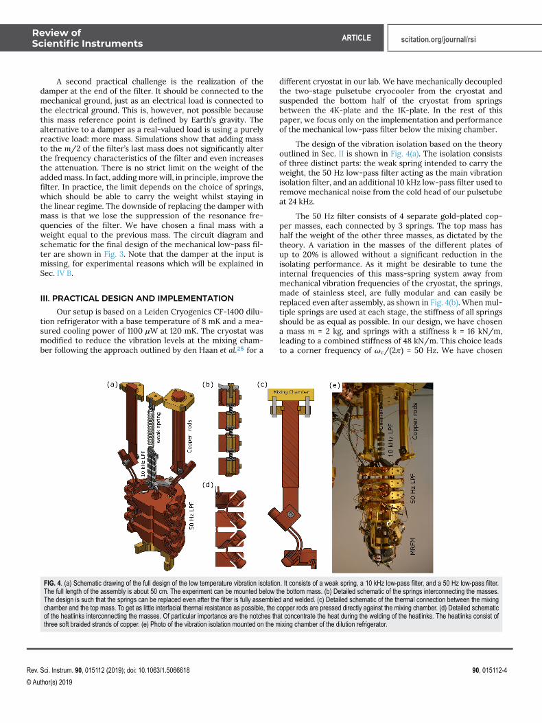
The design of the vibration isolation based on the theoryoutlined in Sec. II is shown in Fig. 4(a). The isolation consistsof three distinct parts: the weak spring intended to carry theweight, the 50 Hz low-pass filter acting as the main vibrationisolation filter, and an additional 10 kHz low-pass filter used toremove mechanical noise from the cold head of our pulsetubeat 24 kHz.

The 50 Hz filter consists of 4 separate gold-plated cop-per masses, each connected by 3 springs. The top mass hashalf the weight of the other three masses, as dictated by thetheory. A variation in the masses of the different plates ofup to 20% is allowed without a significant reduction in theisolating performance. As it might be desirable to tune theinternal frequencies of this mass-spring system away frommechanical vibration frequencies of the cryostat, the springs,made of stainless steel, are fully modular and can easily bereplaced even after assembly, as shown in Fig. 4(b). When mul-tiple springs are used at each stage, the stiffness of all springsshould be as equal as possible. In our design, we have chosena mass m = 2 kg, and springs with a stiffness k = 16 kN/m,leading to a combined stiffness of 48 kN/m. This choice leadsto a corner frequency of ωc/(2π) = 50 Hz. We have chosen

FIG. 4. (a) Schematic drawing of the full design of the low temperature vibration isolation. It consists of a weak spring, a 10 kHz low-pass filter, and a 50 Hz low-pass filter.The full length of the assembly is about 50 cm. The experiment can be mounted below the bottom mass. (b) Detailed schematic of the springs interconnecting the masses.The design is such that the springs can be replaced even after the filter is fully assembled and welded. (c) Detailed schematic of the thermal connection between the mixingchamber and the top mass. To get as little interfacial thermal resistance as possible, the copper rods are pressed directly against the mixing chamber. (d) Detailed schematicof the heatlinks interconnecting the masses. Of particular importance are the notches that concentrate the heat during the welding of the heatlinks. The heatlinks consist ofthree soft braided strands of copper. (e) Photo of the vibration isolation mounted on the mixing chamber of the dilution refrigerator.

Rev. Sci. Instrum. 90, 015112 (2019); doi: 10.1063/1.5066618 90, 015112-4

© Author(s) 2019

Review ofScientific Instruments ARTICLE scitation.org/journal/rsi

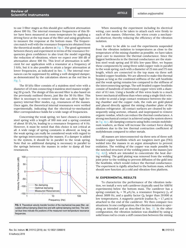
to use 3 filter stages as this should give sufficient attenuationabove 100 Hz. The internal resonance frequencies of this fil-ter have been measured at room temperature by applying adriving force at the top mass of the filter and using geophonesto measure the response at the bottom mass. The frequen-cies match well with the resonance frequencies obtained fromthe theoretical model, as shown in Fig. 5. The good agreementbetween theory and experiment in terms of the resonance fre-quencies gives confidence to also trust the model regardingthe reduction of vibrations, where we expect over 100 dB ofattenuation above 100 Hz. This level of attenuation is suffi-cient for our application with a resonator at a frequency of3 kHz, but it is also possible to attain a larger attenuation atlower frequencies, as indicated in Sec. II. The internal reso-nances can be suppressed by adding a well-designed damper,as demonstrated by the calculation shown as the red line inFig. 5.

The 10 kHz filter consists of a stainless steel wire with adiameter of 1.0 mm connecting 4 stainless steel masses weigh-ing 20 g each. The design of this second filter is also based onthe previously outlined theory, just like the 50 Hz filter. Thisfilter is necessary to remove noise that can drive high fre-quency internal filter modes, e.g., resonances of the masses.Once again, the theoretical internal resonances were verifiedexperimentally, indicating that the electrical-to-mechanicalfilter correspondence holds for a wide range of frequencies.

Concerning the weak spring, we have chosen a stainlesssteel spring with a length of 100 mm and a spring constantof about 10 kN/m, leading to a resonance frequency of 4 Hz.However, it must be noted that this choice is not critical atall. A wide range of spring constants is allowed, as long asthe weak spring can really be considered weak with regard tothe springs interconnecting the masses. If a damper is addedto the system, it should be in parallel to the weak spring.Note that no additional damping is necessary in parallel tothe springs between the masses in order to damp all fourresonances.

FIG. 5. Theoretical velocity transfer function of the mechanical low-pass filter, cal-culated without damping (black line) and with optimal damping (red line). The verti-cal blue lines indicate the positions of the measured room-temperature resonancefrequencies.

When mounting the experiment including its electricalwiring, care needs to be taken to attach each wire firmly toeach of the masses. Otherwise, the wires create a mechani-cal shortcut, thereby reducing the efficiency of the vibrationisolation.

In order to be able to cool the experiments suspendedfrom the vibration isolation to temperatures as close to thetemperature of the mixing chamber as possible, we have takengreat care to maximize the thermal conductance. Since thebiggest bottlenecks in the thermal conductance are the stain-less steel weak spring and 10 kHz low-pass filter, we bypassthese components by using three solid copper rods in parallelto the weak spring, each with a diameter of 25 mm and 175 mmlength, which are connected to the top mass via three softbraided copper heatlinks. We are allowed to make this thermalbypass as long as the combined stiffness of the soft heatlinksand the weak spring remains low compared to the stiffness ofthe interconnecting springs. The soft braided copper heatlinksconsist of hundreds of intertwined copper wires with a diam-eter of 0.1 mm. Using a bundle of thin wires leads to a muchlower mechanical stiffness than when using a single thick wire.In order to avoid a large contact resistance between the mix-ing chamber and the copper rods, the rods are gold-platedand placed directly against the mixing chamber plate of thedilution refrigerator. All contact surfaces are cleaned by sub-sequently using acetone, ethanol, and isopropanol to removeorganic residue, which can reduce the thermal conductance. Astrong mechanical contact is achieved using the system shownin Fig. 4(c). All clamping contacts using bolts contain molybde-num washers, as these will increase the contact force duringcooldown due to the low thermal contraction coefficient ofmolybdenum compared to other metals.

All masses are interconnected via three sets of three softbraided copper heatlinks which are tungsten inert gas (TIG)welded into the masses in an argon atmosphere to preventoxidation. The welding of the copper was made possible bythe notched structure of the welding joints in the masses [seeFig. 4(d)], which are intended to concentrate the heat dur-ing welding. The gold plating was removed from the weldingjoint prior to the welding to prevent diffusion of the gold intothe heatlinks, which would reduce the thermal conductance.The experiment is rigidly attached to the bottom mass, whichshould now function as a cold and vibration-free platform.

IV. EXPERIMENTAL RESULTSTo characterize the performance of the vibration isola-

tion, we install a very soft cantilever (typically used for MRFMexperiments) below the bottom mass. The cantilever has aspring constant k0 = 70 µN/m, a resonance frequency f0 ofabout 3009 Hz, and a quality factor Q0 larger than 20 000 atlow temperatures. A magnetic particle (radius R0 = 1.7 µm) isattached to the end of the cantilever. We then compare twosituations: In one configuration, the vibration isolation is oper-ating as intended and as described in Sec. III. In the otherconfiguration, the vibration isolation was disabled by using asolid brass rod to create a stiff connection between the mixing

Rev. Sci. Instrum. 90, 015112 (2019); doi: 10.1063/1.5066618 90, 015112-5

© Author(s) 2019

Review ofScientific Instruments ARTICLE scitation.org/journal/rsi

chamber and the last mass of the vibration isolation. This sim-ulates a situation where the experiment is mounted withoutvibration isolation. The vibrations of the setup are determinedby measuring the motion of the cantilever using a supercon-ducting quantum interference device (SQUID),37 which mea-sures the changing flux due to the motion of the particle. Thesensitivity of this vibration measurement is limited by the fluxnoise of the SQUID, which can be converted to a displace-ment noise using the thermal motion of the cantilever andthe equipartition theorem.34 We start by demonstrating thethermal properties of the vibration isolation.

A. Thermal conductanceTo verify the effectiveness of the thermalization, we have

measured the heat conductance of our vibration isolation. Forthe base temperature of our cryostat, which is a mixing cham-ber temperature of approximately 8 mK, we find that the bot-tom mass of the vibration isolation saturates at 10.5 mK. Thisalready indicates a good performance of the thermalization.We then use a heater to apply a known power to the bottommass, while we again measure the temperature of the bottommass and the mixing chamber. This allows us to quantify aneffective cooling power at the bottom mass (defined as themaximum power that can be dissipated to remain at a set tem-perature). At 100 mK, we measure a cooling power of 113 µW,which is significantly higher than that of comparable softlow temperature vibration isolations described in the litera-ture,2,32 and only about a factor of 7 lower than the coolingpower of the mixing chamber of the dilution refrigerator atthe same temperature.

The experimental data are compared to a finite elementsimulation using Comsol Multiphysics to determine the limit-ing factors in the heat conductance. The results of this analysisand the experimental data are shown in Fig. 6. We use a ther-mal conductivity that is linearly dependent on temperature as

expected for metals,38 given by κ = 145 · T. The proportionalityconstant of 145 W m−1 K−2 corresponds to low purity cop-per.39 The simulated temperature distribution (for an inputpower of 5.4 mW) is shown in Fig. 6(a). The uniformity of thecolor of the masses indicates that the heatlinks interconnect-ing the masses are the limiting thermal resistance, somethingthat becomes even more apparent from the plotted thermalgradient as shown in Fig. 6(b).

There is a good correspondence between the simulationand the experimental values for all applied powers, as shownin Fig. 6(c). Similar agreement is found when plotting the heatconductance between the bottom mass and the mixing cham-ber as a function of the temperature of the bottom mass[Fig. 6(d)]. The assumption that the heat conductivity is lin-early dependent on the temperature seems to hold over thefull temperature range. As the model does not include con-tact resistance or radiation, but only the geometry and ther-mal properties of the copper, we can conclude that the ther-mal performance of the vibration isolation is limited purelyby the thermal conductance of the braided copper. Further-more, we do not expect that other sources of thermal resis-tance follow this particular temperature dependence.38 So,the argon-welded connections appear to be of sufficient qual-ity not the hinder the conductance. The performance can beimproved further by making the heatlinks out of copper witha higher residual resistivity ratio (RRR) value and thereby ahigher thermal conductivity.

B. SQUID vibration spectrumThe performance of the vibration isolation is shown in

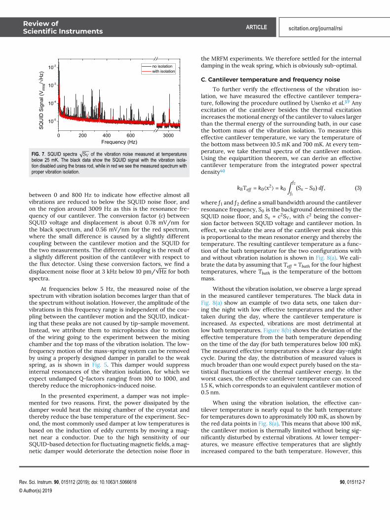
Fig. 7, where we plot the measured SQUID spectra for the twodifferent situations: In the red data, the vibration isolation isin full operation. The black data show the situation when thevibration isolation is disabled. A clear improvement is visiblefor nearly all frequencies above 5 Hz. We focus on the region

FIG. 6. Measurements and finite element simulations of the thermal properties of the vibration isolation. A power is applied to the bottom mass, and the temperature of thebottom mass and the mixing chamber are measured. In the simulation, we insert the power and mixing chamber temperature and calculate the corresponding temperatureof the bottom mass to check the model. Results of the simulation for the (a) temperature and (b) temperature gradient are shown for a power of 5.4 mW. (c) Measuredtemperature of the mixing chamber and bottom mass as a function of the applied power. The solid lines are the simulated temperatures at each of the masses (red is thebottom mass, blue is the bottom of the copper rod). At 100 mK, we find a cooling power of 113 µW at the bottom mass. (d) Heat conductance between the bottom mass andthe mixing chamber as a function of the temperature of the bottom mass. The solid line is a linear fit to the data.

Rev. Sci. Instrum. 90, 015112 (2019); doi: 10.1063/1.5066618 90, 015112-6

© Author(s) 2019

Review ofScientific Instruments ARTICLE scitation.org/journal/rsi

FIG. 7. SQUID spectra√SV of the vibration noise measured at temperatures

below 25 mK. The black data show the SQUID signal with the vibration isola-tion disabled using the brass rod, while in red we see the measured spectrum withproper vibration isolation.

between 0 and 800 Hz to indicate how effective almost allvibrations are reduced to below the SQUID noise floor, andon the region around 3009 Hz as this is the resonance fre-quency of our cantilever. The conversion factor (c) betweenSQUID voltage and displacement is about 0.78 mV/nm forthe black spectrum, and 0.56 mV/nm for the red spectrum,where the small difference is caused by a slightly differentcoupling between the cantilever motion and the SQUID forthe two measurements. The different coupling is the result ofa slightly different position of the cantilever with respect tothe flux detector. Using these conversion factors, we find adisplacement noise floor at 3 kHz below 10 pm/

√Hz for both

spectra.

At frequencies below 5 Hz, the measured noise of thespectrum with vibration isolation becomes larger than that ofthe spectrum without isolation. However, the amplitude of thevibrations in this frequency range is independent of the cou-pling between the cantilever motion and the SQUID, indicat-ing that these peaks are not caused by tip-sample movement.Instead, we attribute them to microphonics due to motionof the wiring going to the experiment between the mixingchamber and the top mass of the vibration isolation. The low-frequency motion of the mass-spring system can be removedby using a properly designed damper in parallel to the weakspring, as is shown in Fig. 5. This damper would suppressinternal resonances of the vibration isolation, for which weexpect undamped Q-factors ranging from 100 to 1000, andthereby reduce the microphonics-induced noise.

In the presented experiment, a damper was not imple-mented for two reasons. First, the power dissipated by thedamper would heat the mixing chamber of the cryostat andthereby reduce the base temperature of the experiment. Sec-ond, the most commonly used damper at low temperatures isbased on the induction of eddy currents by moving a mag-net near a conductor. Due to the high sensitivity of ourSQUID-based detection for fluctuating magnetic fields, a mag-netic damper would deteriorate the detection noise floor in

the MRFM experiments. We therefore settled for the internaldamping in the weak spring, which is obviously sub-optimal.

C. Cantilever temperature and frequency noiseTo further verify the effectiveness of the vibration iso-

lation, we have measured the effective cantilever tempera-ture, following the procedure outlined by Usenko et al.37 Anyexcitation of the cantilever besides the thermal excitationincreases the motional energy of the cantilever to values largerthan the thermal energy of the surrounding bath, in our casethe bottom mass of the vibration isolation. To measure thiseffective cantilever temperature, we vary the temperature ofthe bottom mass between 10.5 mK and 700 mK. At every tem-perature, we take thermal spectra of the cantilever motion.Using the equipartition theorem, we can derive an effectivecantilever temperature from the integrated power spectraldensity40

kBTeff = k0〈x2〉 = k0

∫ f2

f1(Sx − S0) df, (3)

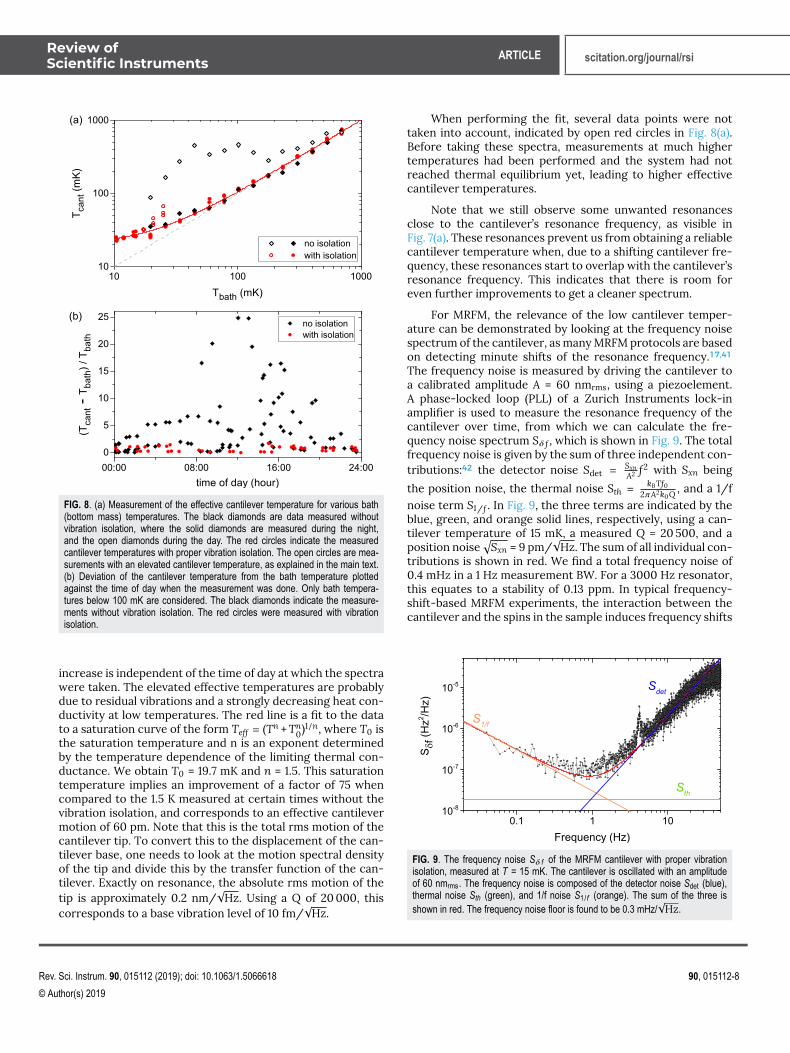
where f1 and f2 define a small bandwidth around the cantileverresonance frequency, S0 is the background determined by theSQUID noise floor, and Sx = c2SV , with c2 being the conver-sion factor between SQUID voltage and cantilever motion. Ineffect, we calculate the area of the cantilever peak since thisis proportional to the mean resonator energy and thereby thetemperature. The resulting cantilever temperature as a func-tion of the bath temperature for the two configurations withand without vibration isolation is shown in Fig. 8(a). We cali-brate the data by assuming that Teff = Tbath for the four highesttemperatures, where Tbath is the temperature of the bottommass.

Without the vibration isolation, we observe a large spreadin the measured cantilever temperatures. The black data inFig. 8(a) show an example of two data sets, one taken dur-ing the night with low effective temperatures and the othertaken during the day, where the cantilever temperature isincreased. As expected, vibrations are most detrimental atlow bath temperatures. Figure 8(b) shows the deviation of theeffective temperature from the bath temperature dependingon the time of the day (for bath temperatures below 100 mK).The measured effective temperatures show a clear day-nightcycle. During the day, the distribution of measured values ismuch broader than one would expect purely based on the sta-tistical fluctuations of the thermal cantilever energy. In theworst cases, the effective cantilever temperature can exceed1.5 K, which corresponds to an equivalent cantilever motion of0.5 nm.

When using the vibration isolation, the effective can-tilever temperature is nearly equal to the bath temperaturefor temperatures down to approximately 100 mK, as shown bythe red data points in Fig. 8(a). This means that above 100 mK,the cantilever motion is thermally limited without being sig-nificantly disturbed by external vibrations. At lower temper-atures, we measure effective temperatures that are slightlyincreased compared to the bath temperature. However, this

Rev. Sci. Instrum. 90, 015112 (2019); doi: 10.1063/1.5066618 90, 015112-7

© Author(s) 2019

Review ofScientific Instruments ARTICLE scitation.org/journal/rsi

FIG. 8. (a) Measurement of the effective cantilever temperature for various bath(bottom mass) temperatures. The black diamonds are data measured withoutvibration isolation, where the solid diamonds are measured during the night,and the open diamonds during the day. The red circles indicate the measuredcantilever temperatures with proper vibration isolation. The open circles are mea-surements with an elevated cantilever temperature, as explained in the main text.(b) Deviation of the cantilever temperature from the bath temperature plottedagainst the time of day when the measurement was done. Only bath tempera-tures below 100 mK are considered. The black diamonds indicate the measure-ments without vibration isolation. The red circles were measured with vibrationisolation.

increase is independent of the time of day at which the spectrawere taken. The elevated effective temperatures are probablydue to residual vibrations and a strongly decreasing heat con-ductivity at low temperatures. The red line is a fit to the datato a saturation curve of the form Teff = (Tn +Tn

0)1/n, where T0 isthe saturation temperature and n is an exponent determinedby the temperature dependence of the limiting thermal con-ductance. We obtain T0 = 19.7 mK and n = 1.5. This saturationtemperature implies an improvement of a factor of 75 whencompared to the 1.5 K measured at certain times without thevibration isolation, and corresponds to an effective cantilevermotion of 60 pm. Note that this is the total rms motion of thecantilever tip. To convert this to the displacement of the can-tilever base, one needs to look at the motion spectral densityof the tip and divide this by the transfer function of the can-tilever. Exactly on resonance, the absolute rms motion of thetip is approximately 0.2 nm/

√Hz. Using a Q of 20 000, this

corresponds to a base vibration level of 10 fm/√

Hz.

When performing the fit, several data points were nottaken into account, indicated by open red circles in Fig. 8(a).Before taking these spectra, measurements at much highertemperatures had been performed and the system had notreached thermal equilibrium yet, leading to higher effectivecantilever temperatures.

Note that we still observe some unwanted resonancesclose to the cantilever’s resonance frequency, as visible inFig. 7(a). These resonances prevent us from obtaining a reliablecantilever temperature when, due to a shifting cantilever fre-quency, these resonances start to overlap with the cantilever’sresonance frequency. This indicates that there is room foreven further improvements to get a cleaner spectrum.

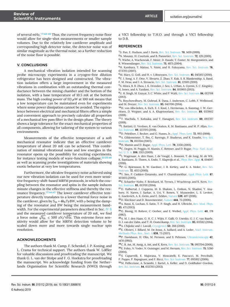
For MRFM, the relevance of the low cantilever temper-ature can be demonstrated by looking at the frequency noisespectrum of the cantilever, as many MRFM protocols are basedon detecting minute shifts of the resonance frequency.17,41The frequency noise is measured by driving the cantilever toa calibrated amplitude A = 60 nmrms, using a piezoelement.A phase-locked loop (PLL) of a Zurich Instruments lock-inamplifier is used to measure the resonance frequency of thecantilever over time, from which we can calculate the fre-quency noise spectrum Sδ f , which is shown in Fig. 9. The totalfrequency noise is given by the sum of three independent con-tributions:42 the detector noise Sdet =

SxnA2 f2 with Sxn being

the position noise, the thermal noise Sth =kBTf0

2πA2k0Q, and a 1/f

noise term S1/f . In Fig. 9, the three terms are indicated by theblue, green, and orange solid lines, respectively, using a can-tilever temperature of 15 mK, a measured Q = 20 500, and aposition noise

√Sxn = 9 pm/

√Hz. The sum of all individual con-

tributions is shown in red. We find a total frequency noise of0.4 mHz in a 1 Hz measurement BW. For a 3000 Hz resonator,this equates to a stability of 0.13 ppm. In typical frequency-shift-based MRFM experiments, the interaction between thecantilever and the spins in the sample induces frequency shifts

FIG. 9. The frequency noise Sδ f of the MRFM cantilever with proper vibrationisolation, measured at T = 15 mK. The cantilever is oscillated with an amplitudeof 60 nmrms. The frequency noise is composed of the detector noise Sdet (blue),thermal noise Sth (green), and 1/f noise S1/ f (orange). The sum of the three isshown in red. The frequency noise floor is found to be 0.3 mHz/

√Hz.

Rev. Sci. Instrum. 90, 015112 (2019); doi: 10.1063/1.5066618 90, 015112-8

© Author(s) 2019

Review ofScientific Instruments ARTICLE scitation.org/journal/rsi

of several mHz.17,43–45 Thus, the current frequency noise floorwould allow for single-shot measurements or smaller samplevolumes. Due to the relatively low cantilever amplitude andcorresponding high detector noise, the detector noise was ofsimilar magnitude as the thermal noise, so a further reductionof the noise floor is possible.

V. CONCLUSIONSA mechanical vibration isolation intended for scanning

probe microscopy experiments in a cryogen-free dilutionrefrigerator has been designed and constructed. The vibra-tion isolation offers a large improvement in the measuredvibrations in combination with an outstanding thermal con-ductance between the mixing chamber and the bottom of theisolation, with a base temperature of 10.5 mK at the bottommass. The high cooling power of 113 µW at 100 mK means thata low temperature can be maintained even for experimentswhere some power dissipation cannot be avoided. The equiva-lence between electrical and mechanical filters offers a simpleand convenient approach to precisely calculate all propertiesof a mechanical low pass filter in the design phase. The theoryshows a large tolerance for the exact mechanical properties ofall components, allowing for tailoring of the system to variousenvironments.

Measurements of the effective temperature of a softmechanical resonator indicate that an effective cantilevertemperature of about 20 mK can be achieved. This combi-nation of minimal vibrational noise and low energies in theresonator opens up the possibility for exciting experiments,for instance testing models of wave-function collapse,22,23,46as well as scanning probe investigations of materials showingexotic behavior at very low temperatures.

Furthermore, the ultralow frequency noise achieved usingour new vibration isolation can be used for even more sensi-tive frequency-shift-based MRFM protocols, in which the cou-pling between the resonator and spins in the sample inducesminute changes in the effective stiffness and thereby the res-onance frequency.17,44,47 The lower cantilever effective tem-perature directly translates to a lower thermal force noise inthe cantilever, given by Sth = 4kBTγBW, with γ being the damp-ing of the resonator and BW being the measurement band-width. For the experimental parameters described in Sec. IV Band the measured cantilever temperature of 20 mK, we finda force noise

√Sth . 500 zN/

√Hz. This extreme force sen-

sitivity would allow for the MRFM detection volume to bescaled down more and more towards single nuclear spinresolution.

ACKNOWLEDGMENTSThe authors thank M. Camp, F. Schenkel, J. P. Koning, and

L. Crama for technical support. The authors thank W. Löfflerfor valuable discussions and proofreading the manuscript. Wethank G. L. van der Stolpe and F. G. Hoekstra for proofreadingthe manuscript. We acknowledge funding from the Nether-lands Organisation for Scientific Research (NWO) through

a VICI fellowship to T.H.O. and through a VICI fellowshipto D.B.

REFERENCES1S. Pan, E. Hudson, and J. Davis, Rev. Sci. Instrum. 70, 1459 (1999).2N. Moussy, H. Courtois, and B. Pannetier, Rev. Sci. Instrum. 72, 128 (2001).3J. Wiebe, A. Wachowiak, F. Meier, D. Haude, T. Foster, M. Morgenstern, andR. Wiesendanger, Rev. Sci. Instrum. 75, 4871 (2004).4H. Kambara, T. Matsui, Y. Niimi, and H. Fukuyama, Rev. Sci. Instrum. 78,073703 (2007).5M. Marz, G. Goll, and H. v. Löhneysen, Rev. Sci. Instrum. 81, 045102 (2010).6Y. J. Song, A. F. Otte, V. Shvarts, Z. Zhao, Y. Kuk, S. R. Blankenship, A. Band,F. M. Hess, and J. A. Stroscio, Rev. Sci. Instrum. 81, 121101 (2010).7S. Misra, B. B. Zhou, I. K. Drozdov, J. Seo, L. Urban, A. Gyenis, S. C. Kingsley,H. Jones, and A. Yazdani, Rev. Sci. Instrum. 84, 103903 (2013).8U. R. Singh, M. Enayat, S. C. White, and P. Wahl, Rev. Sci. Instrum. 84, 013708(2013).9A. Roychowdhury, M. Gubrud, R. Dana, J. Anderson, C. Lobb, F. Wellstood,and M. Dreyer, Rev. Sci. Instrum. 85, 043706 (2014).10H. von Allwörden, A. Eich, E. J. Knol, J. Hermenau, A. Sonntag, J. W. Ger-ritsen, D. Wegner, and A. A. Khajetoorians, Rev. Sci. Instrum. 89, 033902(2018).11T. Machida, Y. Kohsaka, and T. Hanaguri, Rev. Sci. Instrum. 89, 093707(2018).12I. Battisti, G. Verdoes, K. van Oosten, K. M. Bastiaans, and M. P. Allan, Rev.Sci. Instrum. 89, 123705 (2018).13D. Pelekhov, J. Becker, and G. Nunes, Jr., Appl. Phys. Lett. 72, 993 (1998).14A. Gildemeister, T. Ihn, C. Barengo, P. Studerus, and K. Ensslin, Rev. Sci.Instrum. 78, 013704 (2007).15H. Mamin and D. Rugar, Appl. Phys. Lett. 79, 3358 (2001).16C. Degen, M. Poggio, H. Mamin, C. Rettner, and D. Rugar, Proc. Natl. Acad.Sci. U. S. A. 106, 1313 (2009).17J. Wagenaar, A. den Haan, J. de Voogd, L. Bossoni, T. de Jong, M. de Wit,K. Bastiaans, D. Thoen, A. Endo, T. Klapwijk et al., Phys. Rev. Appl. 6, 014007(2016).18P. G. Björnsson, B. W. Gardner, J. R. Kirtley, and K. A. Moler, Rev. Sci.Instrum. 72, 4153 (2001).19Y. Seo, P. Cadden-Zimansky, and V. Chandrasekhar, Appl. Phys. Lett. 87,103103 (2005).20E. Schaefer-Nolte, F. Reinhard, M. Ternes, J. Wrachtrup, and K. Kern, Rev.Sci. Instrum. 85, 013701 (2014).21D. Halbertal, J. Cuppens, M. B. Shalom, L. Embon, N. Shadmi, Y. Ana-hory, H. Naren, J. Sarkar, A. Uri, Y. Ronen, Y. Myasoedov, L. S. Levitov,E. Joselevich, A. K. Geim, and E. Zeldov, Nature 539, 407 (2016).22D. Kleckner and D. Bouwmeester, Nature 444, 75 (2006).23A. Bassi, K. Lochan, S. Satin, T. P. Singh, and H. Ulbricht, Rev. Mod. Phys.85, 471 (2013).24G. Binnig, H. Rohrer, C. Gerber, and E. Weibel, Appl. Phys. Lett. 40, 178(1982).25A. M. J. den Haan, G. H. C. J. Wijts, F. Galli, O. Usenko, G. J. C. van Baarle,D. J. van der Zalm, and T. H. Oosterkamp, Rev. Sci. Instrum. 85, 035112 (2014).26A. Chijioke and J. Lawall, Cryogenics 50, 266 (2010).27E. Olivieri, J. Billard, M. De Jesus, A. Juillard, and A. Leder, Nucl. Instrum.Methods Phys. Res., Sect. A 858, 73 (2017).28P. Davidsson, H. Olin, M. Persson, and S. Pehrson, Ultramicroscopy 42,1470 (1992).29C. R. Ast, M. Assig, A. Ast, and K. Kern, Rev. Sci. Instrum. 79, 093704 (2008).30E. Foley, N. Yoder, N. Guisinger, and M. Hersam, Rev. Sci. Instrum. 75, 5280(2004).31S. Caparrelli, E. Majorana, V. Moscatelli, E. Pascucci, M. Perciballi,P. Puppo, P. Rapagnani, and F. Ricci, Rev. Sci. Instrum. 77, 095102 (2006).32M. Pelliccione, A. Sciambi, J. Bartel, A. Keller, and D. Goldhaber-Gordon,Rev. Sci. Instrum. 84, 033703 (2013).

Rev. Sci. Instrum. 90, 015112 (2019); doi: 10.1063/1.5066618 90, 015112-9

© Author(s) 2019

Review ofScientific Instruments ARTICLE scitation.org/journal/rsi

33M. Poggio and C. Degen, Nanotechnology 21, 342001 (2010).34A. Vinante, A. Kirste, A. den Haan, O. Usenko, G. Wijts, E. Jeffrey,P. Sonin, D. Bouwmeester, and T. Oosterkamp, Appl. Phys. Lett. 101, 123101(2012).35G. R. Fowles and G. L. Cassiday, Analytical Mechanics, 7th ed. (ThomsonLearning, Inc., 2005).36G. A. Campbell, “Electrical receiving, translating, or repeating circuit,”U.S. patent US1227114A (22 May 1917).37O. Usenko, A. Vinante, G. Wijts, and T. Oosterkamp, Appl. Phys. Lett. 98,133105 (2011).38F. Pobell, Matter and Methods at Low Temperatures (Springer, 1996), Vol. 2.39A. L. Woodcraft, Cryogenics 45, 626 (2005).40M. Aspelmeyer, T. J. Kippenberg, and F. Marquardt, Rev. Mod. Phys. 86,1391 (2014).

41H. J. Mamin, M. Poggio, C. L. Degen, and D. Rugar, Nat. Nanotechnol. 2,301 (2007).42S. M. Yazdanian, J. A. Marohn, and R. F. Loring, J. Chem. Phys. 128, 224706(2008).43D. Rugar, R. Budakian, H. J. Mamin, and B. W. Chui, Nature 430, 329(2004).44S. R. Garner, S. Kuehn, J. M. Dawlaty, N. E. Jenkins, and J. A. Marohn, Appl.Phys. Lett. 84, 5091 (2004).45D. A. Alexson, S. A. Hickman, J. A. Marohn, and D. D. Smith, Appl. Phys.Lett. 101, 022103 (2012).46A. Vinante, M. Bahrami, A. Bassi, O. Usenko, G. Wijts, and T. Oosterkamp,Phys. Rev. Lett. 116, 090402 (2016).47L. Chen, J. G. Longenecker, E. W. Moore, and J. A. Marohn, Appl. Phys. Lett.102, 132404 (2013).

Rev. Sci. Instrum. 90, 015112 (2019); doi: 10.1063/1.5066618 90, 015112-10

© Author(s) 2019