vibration control with shape-memory alloys · vibration control with shape-memory alloys ... work...
TRANSCRIPT
VIBRATION CONTROL WITH
SHAPE-MEMORY ALLOYS
IN CIVIL ENGINEERING STRUCTURES
Filipe Pimentel Amarante dos Santos
Mestre em Engenharia de Estruturas
Dissertacao apresentada a Faculdade de Ciencias e
Tecnologia da Universidade Nova de Lisboa para obtencao
do grau de Doutor em Engenharia Civil
Orientador: Professor Doutor Corneliu Cismasiu
Juri:
Presidente: Professor Doutor Manuel Americo Goncalves da Silva
Arguente: Professor Doutor Alvaro Alberto de Matos Ferreira da Cunha
Arguente: Professor Doutor Luıs Manuel Coelho Guerreiro
Vogal: Professor Doutor Antonio Jose Luıs dos Reis
Vogal: Professor Doutor Joao Carlos Gomes Rocha de Almeida
Marco 2011


“Copyright” Filipe Pimentel Amarante dos Santos, FCT/UNL e UNL
A Faculdade de Ciencias e Tecnologia e a Universidade Nova de Lisboa tem o direito,
perpetuo e sem limites geograficos, de arquivar e publicar esta dissertacao atraves
de exemplares impressos reproduzidos em papel ou de forma digital, ou por qual-
quer outro meio conhecido ou que venha a ser inventado, e de a divulgar atraves de
repositorios cientıficos e de admitir a sua copia e distribuicao com objectivos edu-
cacionais ou de investigacao, nao comerciais, desde que seja dado credito ao autor e
editor.


To my wife Ines and our son Afonso


Acknowledgments
This dissertation would not have been accomplished without the support and assis-
tance from many people in many different ways.
I would like to express my deepest and heartfelt recognition to my adviser, Prof.
Corneliu Cismasiu. I cannot thank him enough for his priceless scientific teachings,
for his invaluable guidance and commitment, for his inestimable encouragement,
confidence and utmost support, and last but not the least, for his enormous gen-
erosity and kind friendship, which have made this graduation experience so positive
and so meaningful. To work with him was a great pleasure and a privilege.
I am truly and forever grateful to Prof. J. Pamies Teixeira for his incalculable help
during the design and construction phases of the physical prototype. Without his
inspired input and thoughtful dedication the interdisciplinary nature of this study
could not have been achieved.
I would like to show my true appreciation to Prof. F. M. Bras Fernandes, who first
brought me into the shape-memory world and with whom I had so many fruitful
and delightful discussions, and to K.K. Mahesh for his precious help during the DSC
tests.
I would like to thank Prof. Fernando Coito for his availability and for his insightful
explanations about modern control engineering.
I am also indebted to Prof. J. C. G. Rocha de Almeida and I profoundly thank him
for his unconditional support in overcoming all the bureaucratic perils that have
appeared along the way.
I thank Prof. M. Goncalves da Silva for his warm welcome to the Civil Enginnering
Department and for his relentless efforts in providing me with the necessary logistic
i

conditions to pursuit this work.
I kindly acknowledge Prof. F. Henriques for the use of the infrared camera, during
the study of the transformation fronts.
I thank Prof. Antonio Reis for introducing me to scientific investigation, for inciting
my natural curiosity in the pursuit of further knowledge and for motivating me to
continue my academic studies. I am also grateful to him for the technical data
regarding the S. Martinho viaduct.
To my colleagues and friends I thank for all the good disposition and support.
I specially would like to thank my good friend Mario Silva for his priceless technical
support with Linux, always managing to solve the innumerable helpless situations I
found myself into during the coarse of this work. I also thank him and Jose Varandas
for all the waves I had the pleasure of sharing with them and for all the laughter.
I thank my parents for all their love and everlasting devotion.
Finally, all my love goes to Ines and Afonso as they are the bright sunshine of my
life.
I acknowledge the financial support of Fundacao Calouste Gulbenkian (bolsa de
curta duracao) and of Fundacao para a Ciencia e Tecnologia (FCT/MCTES grant
SFRH/BD/37653/2007).
Abstract
The superelastic behavior exhibited by shape-memory alloys shows a vast potential
for technological applications in the field of seismic hazard mitigation, for civil engi-
neering structures. Due to this property, the material is able to totally recover from
large cyclic deformations, while developing a hysteretic loop. This is translated into
a high inherent damping, combined with repeatable re-centering capabilities, two
fundamental features of vibration control devices.
An extensive experimental program provides a valuable insight into the identification
of the main variables influencing superelastic damping in Nitinol while exploring the
feasibility and optimal behavior of SMAs when used in seismic vibration control.
The knowledge yielded from the experimental program, together with an extensive
bibliographic research, allows for the development of an efficient numerical frame-
work for the mathematical modeling of the complex thermo-mechanical behavior of
SMAs. These models couple the mechanical and kinetic transformation constitutive
laws with a heat balance equation describing the convective heat problem. The seis-
mic behavior of a superelastic restraining bridge system is successfully simulated,
being one of the most promising applications regarding the use of SMAs in civil
engineering structures.
A small-scale physical prototype of a novel superelastic restraining device is built.
The device is able to dissipate a considerable amount of energy, while minimizing
a set of adverse effects, related with cyclic loading and aging effects, that hinder
the dynamic performances of vibration control devices based on passive superelastic
wires.
iii

Resumo
O comportamento superelastico desenvolvido pelas ligas com memoria de forma
confere-lhes um vasto potencial no que diz respeito a aplicacoes tecnologicas no
domınio do controlo de vibracoes em estruturas de engenharia civil. Devido a su-
perelasticidade, o material e capaz de recuperar a sua forma original, apos ter sido
submetido a grandes deformacoes, desenvolvendo um comportamento histeretico.
Este comportamento traduz-se numa capacidade de amortecimento intrınseca que,
conjuntamente com as elevadas capacidades de reposicionamento do material, con-
stituem caracterısticas fundamentais para a eficacia de um dispositivo de controlo
de vibracoes.
E apresentado um vasto programa experimental que contribui para a identificacao
das principais varaveis que influenciam o amortecimento superelastico do Nitinol,
numa tentativa de explorar e optimizar a possibilidade da aplicacao de ligas com
memoria de forma no controlo estrutural de vibracoes.
E tambem apresentada uma ferramenta numerica para a modelacao matematica
do complexo comportamento termo-mecanico das ligas com memoria de forma. Os
modelos considerados fazem o acoplamento de leis constitutivas que traduzem o seu
comportamento mecanico bem como a cinetica das transformacoes martensıticas,
com uma equacao de balanco energetico. O comportamento sısmico de um disposi-
tivo de retencao superelastico para pontes e testado com sucesso, sendo que se trata
de uma das mais promissoras utilizacoes de elementos superelasticos em estruturas
de engenharia civil.
Finalmente, e apresentado um prototipo a escala reduzida de um dispositivo su-
perelastico para o controlo de vibracoes que, sendo capaz de dissipar uma quanti-
dade apreciavel de energia, permite minimizar uma serie de efeitos adversos ligados
a superelasticidade.
v

Contents
List of Figures xiv
List of Tables xxvii
1 Introduction 1
1.1 Problem Description . . . . . . . . . . . . . . . . . . . . . . . . . . . 1
1.2 Objectives and Scope . . . . . . . . . . . . . . . . . . . . . . . . . . . 3
1.3 Dissertation Outline . . . . . . . . . . . . . . . . . . . . . . . . . . . 4
List of Symbols and Abbreviations 1
2 SMAs in Vibration Control Devices 7
2.1 Introduction . . . . . . . . . . . . . . . . . . . . . . . . . . . . . . . . 7
2.2 General aspects of Shape-Memory alloys . . . . . . . . . . . . . . . . 8
2.2.1 Martensitic transformation . . . . . . . . . . . . . . . . . . . . 8
2.2.2 Superelasticity . . . . . . . . . . . . . . . . . . . . . . . . . . 11
2.2.3 Shape-Memory effect . . . . . . . . . . . . . . . . . . . . . . . 14
2.2.4 Internal friction . . . . . . . . . . . . . . . . . . . . . . . . . . 16
2.3 Vibration control devices . . . . . . . . . . . . . . . . . . . . . . . . . 19
vii
2.4 Seismic mitigation devices based on SMAs . . . . . . . . . . . . . . . 20
2.4.1 Bracing systems . . . . . . . . . . . . . . . . . . . . . . . . . . 21
2.4.2 Base isolation system . . . . . . . . . . . . . . . . . . . . . . . 24
2.4.3 Bridge hinge restrainers . . . . . . . . . . . . . . . . . . . . . 25
2.4.4 Structural connections . . . . . . . . . . . . . . . . . . . . . . 29
2.4.5 Applications in existing civil engineering structures . . . . . . 31
2.5 Constraints of using shape-memory alloys . . . . . . . . . . . . . . . . 36
2.6 Closure . . . . . . . . . . . . . . . . . . . . . . . . . . . . . . . . . . . 37
3 NiTi Shape-Memory Alloys 39
3.1 Introduction . . . . . . . . . . . . . . . . . . . . . . . . . . . . . . . . 39
3.2 Characterization of Nitinol . . . . . . . . . . . . . . . . . . . . . . . . 40
3.2.1 Microstructure . . . . . . . . . . . . . . . . . . . . . . . . . . 40
3.2.2 Tensile properties . . . . . . . . . . . . . . . . . . . . . . . . . 42
3.2.3 Transformation temperatures . . . . . . . . . . . . . . . . . . 44
3.2.4 Clausius-Clapeyron coefficient . . . . . . . . . . . . . . . . . . 46
3.2.5 Influence of ambient temperature on damping . . . . . . . . . 48
3.2.6 Internal loops . . . . . . . . . . . . . . . . . . . . . . . . . . . 50
3.2.7 Influence of strain-amplitude on damping . . . . . . . . . . . . 52
3.2.8 Self-heating on mechanical cycling . . . . . . . . . . . . . . . . 54
3.2.9 Influence of strain-rate on damping . . . . . . . . . . . . . . . 57
3.2.10 Transformation fronts . . . . . . . . . . . . . . . . . . . . . . 59
3.2.11 Cyclic properties . . . . . . . . . . . . . . . . . . . . . . . . . 61
3.2.12 Influence of cycling on damping . . . . . . . . . . . . . . . . . 64
3.2.13 Fatigue properties . . . . . . . . . . . . . . . . . . . . . . . . . 65
3.2.14 Strain-creep and stress-relaxation . . . . . . . . . . . . . . . . 66
3.2.15 Aging effects . . . . . . . . . . . . . . . . . . . . . . . . . . . 68
3.3 Closure . . . . . . . . . . . . . . . . . . . . . . . . . . . . . . . . . . . 72
4 Constitutive Models for SMAs 75
4.1 Introduction . . . . . . . . . . . . . . . . . . . . . . . . . . . . . . . . 75
4.2 Mechanical laws . . . . . . . . . . . . . . . . . . . . . . . . . . . . . . 76
4.2.1 Simple serial model . . . . . . . . . . . . . . . . . . . . . . . . 76
4.2.2 Voight scheme . . . . . . . . . . . . . . . . . . . . . . . . . . . 78
4.2.3 Reuss scheme . . . . . . . . . . . . . . . . . . . . . . . . . . . 79
4.3 Kinetic laws . . . . . . . . . . . . . . . . . . . . . . . . . . . . . . . . 79
4.3.1 Linear transformation kinetic laws . . . . . . . . . . . . . . . . 80
4.3.2 Exponential transformation kinetic laws . . . . . . . . . . . . 81
4.4 Thermal effects . . . . . . . . . . . . . . . . . . . . . . . . . . . . . . 83
4.5 Adopted constitutive models for SMAs . . . . . . . . . . . . . . . . . 87
4.6 Numerical implementation of the models . . . . . . . . . . . . . . . . 88
4.6.1 Numerical implementation of the rate-independent constitu-
tive model . . . . . . . . . . . . . . . . . . . . . . . . . . . . . 88
4.6.2 Algorithm for the rate-independent constitutive model . . . . 91
4.6.3 Numerical implementation of the rate-dependent constitutive
model . . . . . . . . . . . . . . . . . . . . . . . . . . . . . . . 92
4.6.4 Algorithm for the rate-dependent constitutive model . . . . . 95
4.7 Numerical assessment of the models . . . . . . . . . . . . . . . . . . . 99
4.7.1 Quasi-static tests . . . . . . . . . . . . . . . . . . . . . . . . . 100
4.7.2 Dynamic tests . . . . . . . . . . . . . . . . . . . . . . . . . . . 102
4.8 Strain-rate analysis using the rate-dependent model . . . . . . . . . . 107
4.9 Closure . . . . . . . . . . . . . . . . . . . . . . . . . . . . . . . . . . . 109
5 Modeling of SE Vibration Control Devices 111
5.1 Introduction . . . . . . . . . . . . . . . . . . . . . . . . . . . . . . . . 111
5.2 Mathematical modeling of dynamical systems . . . . . . . . . . . . . 112
5.3 Pre-strain in superelastic wires . . . . . . . . . . . . . . . . . . . . . . 113
5.4 Numerical implementation . . . . . . . . . . . . . . . . . . . . . . . . 114
5.4.1 Algorithm to solve the equation of motion . . . . . . . . . . . 115
5.5 Numerical tests . . . . . . . . . . . . . . . . . . . . . . . . . . . . . . 117
5.5.1 Vibration control device with SE wire . . . . . . . . . . . . . . 117
5.5.2 Vibration control device with two pre-strained SE wires work-
ing in phase opposition . . . . . . . . . . . . . . . . . . . . . . 118
5.5.3 Vibration control device with two pre-strained SE wires and
a re-centering element . . . . . . . . . . . . . . . . . . . . . . 121
5.5.4 Influence of the ambient temperature on SE vibration control
devices . . . . . . . . . . . . . . . . . . . . . . . . . . . . . . . 122
5.5.5 Influence of strain-rate on SE vibration control devices . . . . 123
5.5.6 Influence of strain-amplitude on SE vibration control devices . 125
5.5.7 Influence of the constitutive model on the modeling of SE
vibration control devices . . . . . . . . . . . . . . . . . . . . . 126
5.6 SE restrainer cables in a viaduct . . . . . . . . . . . . . . . . . . . . . 129
5.6.1 Seismic analysis of the viaduct with SE restrainer cables . . . 129
5.6.2 Influence of the model on the seismic analysis . . . . . . . . . 132
5.6.3 Influence of the SE restraining area . . . . . . . . . . . . . . . 133
5.7 Closure . . . . . . . . . . . . . . . . . . . . . . . . . . . . . . . . . . . 135
6 Novel SE Device 141
6.1 Introduction . . . . . . . . . . . . . . . . . . . . . . . . . . . . . . . . 141
6.2 Semi-active device under harmonic excitation . . . . . . . . . . . . . 142
6.2.1 Passive system with no pre-strain . . . . . . . . . . . . . . . . 142
6.2.2 Passive system with pre-strain . . . . . . . . . . . . . . . . . . 143
6.2.3 Semi-active system . . . . . . . . . . . . . . . . . . . . . . . . 144
6.3 Semi-active device under seismic excitation . . . . . . . . . . . . . . . 153
6.4 Closure . . . . . . . . . . . . . . . . . . . . . . . . . . . . . . . . . . . 158
7 Prototype of the Novel SE Device 161
7.1 Introduction . . . . . . . . . . . . . . . . . . . . . . . . . . . . . . . . 161
7.2 Building the prototype . . . . . . . . . . . . . . . . . . . . . . . . . . 161
7.2.1 Moving-mass-module . . . . . . . . . . . . . . . . . . . . . . . 163
7.2.1.1 Force-sensors . . . . . . . . . . . . . . . . . . . . . . 164
7.2.1.2 Displacement-sensor . . . . . . . . . . . . . . . . . . 172
7.2.2 Linear actuators . . . . . . . . . . . . . . . . . . . . . . . . . . 173
7.2.2.1 Electromechanical cylinder . . . . . . . . . . . . . . . 174
7.2.2.2 Servo-motor and servo-drive . . . . . . . . . . . . . . 174
7.2.2.3 Mounting system and clamps . . . . . . . . . . . . . 175
7.2.3 Prototype . . . . . . . . . . . . . . . . . . . . . . . . . . . . . 176
7.3 Experimenting the prototype . . . . . . . . . . . . . . . . . . . . . . . 178
7.3.1 General control of the servo-system . . . . . . . . . . . . . . . 178
7.3.1.1 Speed-control mode . . . . . . . . . . . . . . . . . . 179
7.3.2 Stress control in a SE wire . . . . . . . . . . . . . . . . . . . . 180
7.3.2.1 Proportional-plus-integral-plus-derivative (PID) con-
troller . . . . . . . . . . . . . . . . . . . . . . . . . . 180
7.3.2.2 Transient-response analysis . . . . . . . . . . . . . . 182
7.3.2.3 Tuning of the PID controller . . . . . . . . . . . . . 184
7.3.2.4 Sinusoidal stress input (reference signal) . . . . . . . 188
7.3.3 Displacement control for dynamic tensile testing . . . . . . . . 188
7.3.4 SE control system with one restraining element . . . . . . . . 192
7.3.5 SE control system with two restraining elements . . . . . . . . 196
7.4 Closure . . . . . . . . . . . . . . . . . . . . . . . . . . . . . . . . . . . 201
8 Summary, Conclusions and Future Work 203
8.1 Summary and conclusions . . . . . . . . . . . . . . . . . . . . . . . . 203
8.2 Future Work . . . . . . . . . . . . . . . . . . . . . . . . . . . . . . . . 207
A Modeling of control systems 213
A.1 Laplace Transformation . . . . . . . . . . . . . . . . . . . . . . . . . 213
A.1.1 Definition of the Laplace transformation . . . . . . . . . . . . 213
A.1.2 Laplace transforms of several common functions . . . . . . . . 214
A.1.2.1 Step function . . . . . . . . . . . . . . . . . . . . . . 214
A.1.2.2 Ramp function . . . . . . . . . . . . . . . . . . . . . 215
A.1.2.3 Pulse function . . . . . . . . . . . . . . . . . . . . . 216
A.1.2.4 Impulse function . . . . . . . . . . . . . . . . . . . . 216
A.1.3 Laplace transforms properties . . . . . . . . . . . . . . . . . . 218
A.1.3.1 Linearity . . . . . . . . . . . . . . . . . . . . . . . . 218
A.1.3.2 Differentiation and integration . . . . . . . . . . . . 219
A.2 Transfer function . . . . . . . . . . . . . . . . . . . . . . . . . . . . . 220
A.3 Control systems . . . . . . . . . . . . . . . . . . . . . . . . . . . . . . 221
A.4 Basic control actions . . . . . . . . . . . . . . . . . . . . . . . . . . . 224
A.4.1 Proportional control . . . . . . . . . . . . . . . . . . . . . . . 224
A.4.2 Derivative control . . . . . . . . . . . . . . . . . . . . . . . . . 224
A.4.3 Integral control . . . . . . . . . . . . . . . . . . . . . . . . . . 225
A.4.4 Proportional-plus-integral-plus-derivative control . . . . . . . . 225
A.4.5 Ziegler-Nichols tuning of PID controlers . . . . . . . . . . . . 226
Appendix 212
B Implementation of control systems 229
B.1 TTL signal . . . . . . . . . . . . . . . . . . . . . . . . . . . . . . . . 229
B.2 Position-control . . . . . . . . . . . . . . . . . . . . . . . . . . . . . . 230
B.3 Servo-drive specifications . . . . . . . . . . . . . . . . . . . . . . . . . 231
C Virtual instruments 235
C.1 Control of the stress level in a SE wire VI . . . . . . . . . . . . . . . 235
C.2 Displacement control for dynamic tensile testing . . . . . . . . . . . . 238
C.3 SE control system with one restraining element . . . . . . . . . . . . 241

C.4 SE control system with two restraining elements . . . . . . . . . . . . 244
Bibliography 247
Index 265
List of Figures
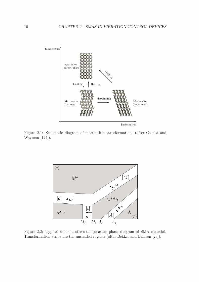
2.1 Schematic diagram of martensitic transformations (after Otsuka and
Wayman [124]). . . . . . . . . . . . . . . . . . . . . . . . . . . . . . . 10
2.2 Typical uniaxial stress-temperature phase diagram of SMA material.
Transformation strips are the unshaded regions (after Bekker and
Brinson [23]). . . . . . . . . . . . . . . . . . . . . . . . . . . . . . . . 10
2.3 Generic stress-strain response of a SMA above Af (adapted from
Shaw and Kyriakides [?]). . . . . . . . . . . . . . . . . . . . . . . . . 12
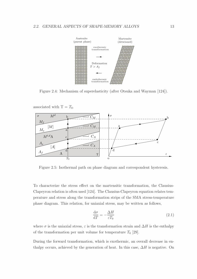
2.4 Mechanism of superelasticity (after Otsuka and Wayman [124]). . . . 13
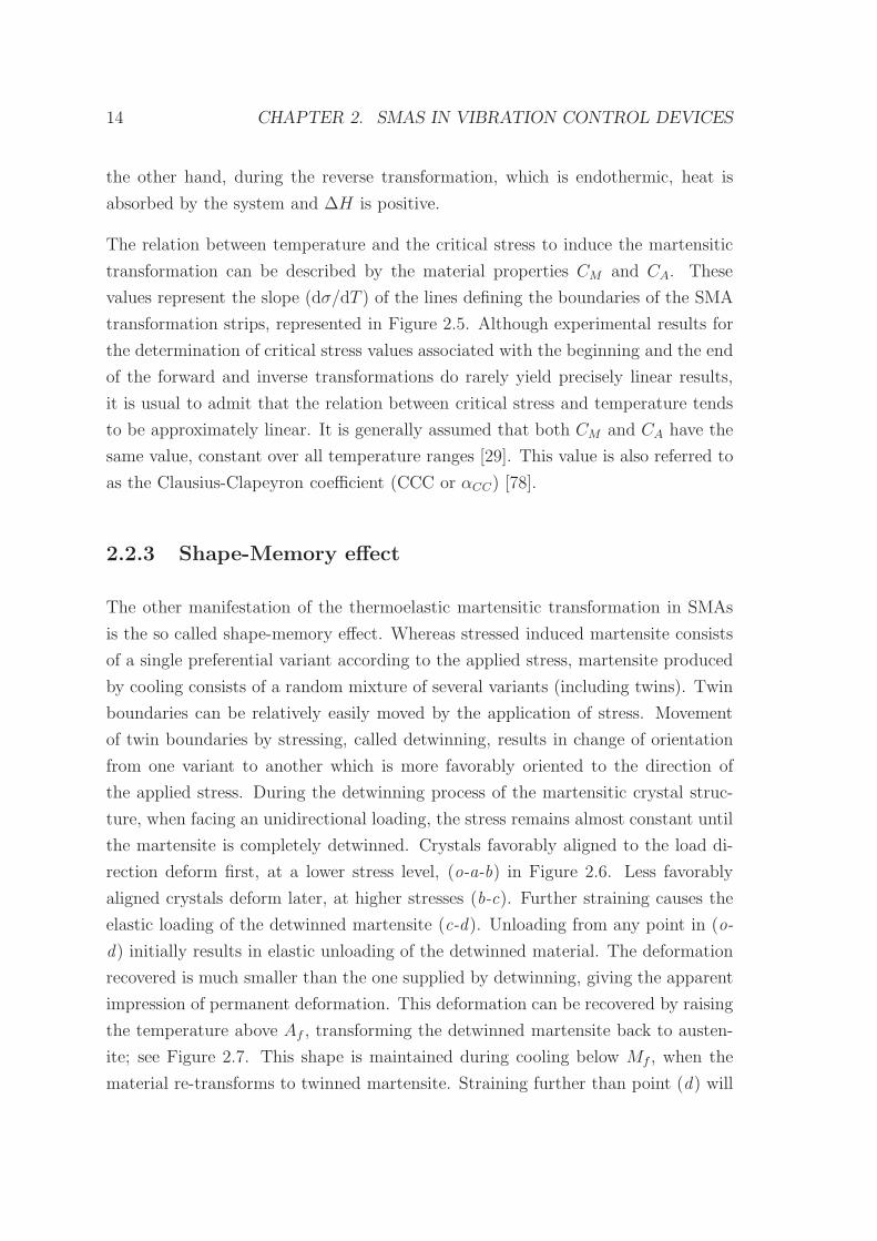
2.5 Isothermal path on phase diagram and correspondent hysteresis. . . . 13
2.6 Generic stress-strain response of a SMA below Mf (adapted from
Shaw and Kyriakides [?]). . . . . . . . . . . . . . . . . . . . . . . . . 15
2.7 Mechanism of shape-memory effect (after Otsuka and Wayman [124]). 15
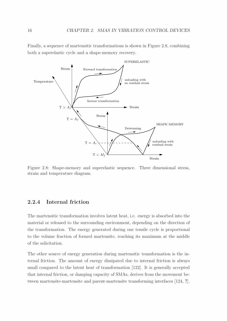
2.8 Shape-memory and superelastic sequence. Three dimensional stress,
strain and temperature diagram. . . . . . . . . . . . . . . . . . . . . . 16
2.9 Definition of energy dissipated ED in a superelastic loading cycle and
maximum strain energy ES0. . . . . . . . . . . . . . . . . . . . . . . . 17
2.10 Small-scale steel framed prototype with SMA braces (adapted from
Boroscheck et al. [27]). . . . . . . . . . . . . . . . . . . . . . . . . . . 22
2.11 SMA-based energy dissipating and re-centering brace (adapted from
Dolce et al. [53]). . . . . . . . . . . . . . . . . . . . . . . . . . . . . . 23
xv
2.12 Adaptive vibration control device for bracing systems (adapted from
Zhang and Zu [177]). . . . . . . . . . . . . . . . . . . . . . . . . . . . 24
2.13 Configuration of elastomeric bearings, friction-pendulum bearings,
SE austenitic wires and magnetorheological dampers. Low-friction
wheels for SMA wire installation (adapted from Shook et al. [149]). . 25
2.14 Unseating of bridge at in-span hinge during an earthquake. . . . . . . 26
2.15 Unseating of bridge at in-span hinge during the 1994 Northridge
earthquake for an existing bridge and a bridge retrofit with tradi-
tional steel restrainer cables (adapted from Johnson et al. [82]). . . . 27
2.16 Restraining solution with SMA elements in a multi-span simply sup-
ported bridge. . . . . . . . . . . . . . . . . . . . . . . . . . . . . . . . 27
2.17 Schematic of the test setup and SMA restrainer cable (adapted from
Johnson et al. [82]). . . . . . . . . . . . . . . . . . . . . . . . . . . . . 28
2.18 SMA restrainer test setup (adapted from Johnson et al. [82]). . . . . 28
2.19 Schematic of the test setup and SMA restrainer cable. Adapted from
Padgett et al. [127]. . . . . . . . . . . . . . . . . . . . . . . . . . . . . 30
2.20 SMA restrainer test setup (adapted from Padgett et al. [127]). . . . . 31
2.21 Schematic of the SMA-based connection test setup (adapted from
Ocel et al. [117]). . . . . . . . . . . . . . . . . . . . . . . . . . . . . . 31
2.22 SMA-based full-scale connection test setup (adapted from Ocel et
al. [117]). . . . . . . . . . . . . . . . . . . . . . . . . . . . . . . . . . 32
2.23 Reinforcement details of beam-column element with coupler (dimen-
sions in mm) (adapted from Alam et al. [5]). . . . . . . . . . . . . . . 32
2.24 Basilica of St. Francis of Assisi in Italy (adapted from [43, 108]). . . . 33
2.25 St. Feliciano Cathedral in Italy (adapted from [35, 108]). . . . . . . . 34
2.26 S. Giorgio Church Bell-Tower in Italy (adapted from [77]). . . . . . . 35
2.27 Bridge carrying Sherman Road over US-31, Michigan, USA (adapted
from [84, 123]). . . . . . . . . . . . . . . . . . . . . . . . . . . . . . . 36
3.1 Austenite unit cell with B2 structure (adapted from[167]). . . . . . . 41
3.2 Schematic view of the B2 → B19’ transformation (adapted from[167]). 41
3.3 Zwick/Roell Z050 testing machine. Gripping apparatus for tensile test. 42
3.4 Stress-strain response of Nitinol wires during uniaxial tensile tests. . . 43
3.5 Stress-strain response during ultimate strength test. . . . . . . . . . . 44
3.6 Schematic illustration of a DSC. Variation in strain during heating
and cooling under constant stress. . . . . . . . . . . . . . . . . . . . . 45
3.7 SETARAM-DSC92 thermal analyzer. General view. . . . . . . . . . . 46
3.8 Temperature controled chamber during the tensile tests. General views. 47
3.9 Temperature dependence of the stress induced martensitic transfor-
mation in a NiTi wire. . . . . . . . . . . . . . . . . . . . . . . . . . . 47
3.10 Variation of ambient temperature. Phase diagram path and corre-
spondent isothermal hysteresis. . . . . . . . . . . . . . . . . . . . . . 48
3.11 Influence of ambient temperature on damping. . . . . . . . . . . . . . 50
3.12 Strain time-histories for internal loop testing in a SE Nitinol wire
sample. . . . . . . . . . . . . . . . . . . . . . . . . . . . . . . . . . . . 51
3.13 Stress-strain diagrams (ε = 0.02%/s). . . . . . . . . . . . . . . . . . . 51
3.14 Variation of strain-amplitude. Phase diagram path and correspondent
isothermal hysteresis. . . . . . . . . . . . . . . . . . . . . . . . . . . . 53
3.15 Influence of strain-amplitude on damping. . . . . . . . . . . . . . . . 54
3.16 Detail of the thermocouple placed in the SE wire. . . . . . . . . . . . 55
3.17 Self heating on mechanical cycling for different strain-rates (T0 =
20C). Temperature time-histories and stress-strain diagrams. . . . . 56
3.18 Temperature variation during a SE mechanical cycle. Phase diagram
path and correspondent isothermal hysteresis. . . . . . . . . . . . . . 58
3.19 Influence of strain-rate on the equivalent viscous damping. . . . . . . 59
3.20 FLIR ThermaCAM B4. . . . . . . . . . . . . . . . . . . . . . . . . . . 59
3.21 Temperature patterns within the SE wire specimen, during the loading-
unloading tensile test (ε = 0.250%/s). . . . . . . . . . . . . . . . . . 60
3.22 Experimental cyclic tensile tests. Stress-strain diagrams. . . . . . . . 62
3.23 Effects of SE cycling. . . . . . . . . . . . . . . . . . . . . . . . . . . . 63
3.24 Experimental cyclic tensile tests. Temperature time-history. . . . . . 64
3.25 Dissipated energy versus the number of cycles at failure [111]. . . . . 66
3.26 Strain-creep and strain-recovery. Phase diagram path and correspon-
dent hysteresis. . . . . . . . . . . . . . . . . . . . . . . . . . . . . . . 67
3.27 Stress-relaxation and stress-recovery. Phase diagram path and corre-
spondent hysteresis. . . . . . . . . . . . . . . . . . . . . . . . . . . . . 68
3.28 Aging under load in the parent phase. Phase diagram path and cor-
respondent hysteresis. . . . . . . . . . . . . . . . . . . . . . . . . . . . 69
3.29 Aging under constant stress in the coexistence zone. Phase diagram
path and correspondent hysteresis. . . . . . . . . . . . . . . . . . . . 70
3.30 Aging under constant strain in the coexistence zone. Phase diagram
path and correspondent hysteresis. . . . . . . . . . . . . . . . . . . . 71
4.1 Mechanical models for SMAs: (a) Simple serial model; (b) Voight
scheme; (c) Reuss scheme. . . . . . . . . . . . . . . . . . . . . . . . . 77
4.2 Superelastic stress-temperature phase plane diagram. Forward (A→
M) and inverse (M → A) transformations. . . . . . . . . . . . . . . . 80
4.3 Cylindrical Nitinol wire surrounded by air. . . . . . . . . . . . . . . . 84
4.4 Description of the constitutive models. . . . . . . . . . . . . . . . . . 87
4.5 Computation of ∆Wn. . . . . . . . . . . . . . . . . . . . . . . . . . . 94
4.6 Computation of the poligonal area. . . . . . . . . . . . . . . . . . . . 98
4.7 Rate-independent numerical model vs. experimental data: quasi-
static loading. . . . . . . . . . . . . . . . . . . . . . . . . . . . . . . . 101
4.8 Rate-dependent numerical model vs. experimental data: quasi-static
loading. . . . . . . . . . . . . . . . . . . . . . . . . . . . . . . . . . . 101
4.9 Rate-dependent numerical model vs. experimental data at tempera-
ture T0 = 20C, for increasing strain-rate (ε). . . . . . . . . . . . . . 104
4.10 Rate-dependent numerical model vs. bibliographic experimental data [51]
for two strain-rates (0.28%/s and 1.40%/s) and four temperatures (10,
20, 30 and 40C). . . . . . . . . . . . . . . . . . . . . . . . . . . . . . 105
4.11 Rate-dependent numerical model vs. bibliographic experimental data [51]:
equivalent viscous damping. . . . . . . . . . . . . . . . . . . . . . . . 106
4.12 Analysis of strain-rate variation at 20C ambient temperature. . . . . 108
4.13 Strain-rate influence on the equivalent viscous damping. . . . . . . . . 108
5.1 SDOF oscillator, with a SE SMA wire acting as restoring element. . . 113
5.2 Difference between a pre-strained SE wire and a non-pre-strained SE
wire subjected to the same strain amplitude: stress-strain relations. . 114
5.3 Average acceleration method, (γ = 1/2 , β = 1/4). . . . . . . . . . . . 114
5.4 Single SE wire (T = 20C, f = 2 Hz). . . . . . . . . . . . . . . . . . . 118
5.5 SDOF oscillator, with two pre-tensioned wires working in phase op-
position. . . . . . . . . . . . . . . . . . . . . . . . . . . . . . . . . . . 119
5.6 Behavior of SE1 and SE2 during generic harmonic cycles. . . . . . . . 119
5.7 Two pre-strained wires working in phase opposition (T = 20C, f = 2 Hz).120
5.8 SDOF oscillator, with two pre-tensioned wires and a re-centering el-
ement. . . . . . . . . . . . . . . . . . . . . . . . . . . . . . . . . . . . 121
5.9 Two pre-tensioned wires with re-centering element (T = 20C, f =
2 Hz). . . . . . . . . . . . . . . . . . . . . . . . . . . . . . . . . . . . 122
5.10 Influence of the ambient temperature on hysteretic cycles. . . . . . . 124
5.11 Influence of the strain-rate on hysteretic cycles. . . . . . . . . . . . . 125
5.12 Influence of the strain-amplitude on hysteretic cycles. . . . . . . . . . 126
5.13 Two pre-tensioned SMA SE wires with re-centering element: (a) dis-
placement time-history; (b) stress time-history; (c) phase-plane; (d)
force-displacement. . . . . . . . . . . . . . . . . . . . . . . . . . . . . 128
5.14 Superelastic restrainer cables at bridge’s supports. . . . . . . . . . . . 129
5.15 Sao Martinho railway viaduct: Mid-span cross section, SMA passive
control device location and finite element model. . . . . . . . . . . . . 130
5.16 Generated accelerograms. . . . . . . . . . . . . . . . . . . . . . . . . . 131
5.17 Longitudinal displacement time-history for free and controlled systems.132
5.18 Longitudinal velocity time-history for free and controlled systems. . . 133
5.19 Longitudinal acceleration time-history for free and controlled systems. 134
5.20 Force in the vibration control device time-history. . . . . . . . . . . . 135
5.21 Time history of the longitudinal displacement of the viaduct deck. . . 136
5.22 Longitudinal displacement and acceleration of the deck in function of
the SE restraining area. . . . . . . . . . . . . . . . . . . . . . . . . . 137
5.23 Longitudinal velocity of the deck and SE force in function of the SE
restraining area. . . . . . . . . . . . . . . . . . . . . . . . . . . . . . . 138
5.24 Parametric curves in function of the SE restraining area. . . . . . . . 139
6.1 Passive system with no pre-strain subjected to an harmonic load.
Strain and displacement time-histories. . . . . . . . . . . . . . . . . . 142
6.2 Passive system with pre-strain subjected to an harmonic load. Strain
and displacement time histories. . . . . . . . . . . . . . . . . . . . . . 143
6.3 Generic functional scheme of the passive and the semi-active systems:
SE wires (SE1 and SE2), supports (S1 and S2) and markers (M1 and
M2). . . . . . . . . . . . . . . . . . . . . . . . . . . . . . . . . . . . . 145
6.4 Block diagram of the on-off control system. . . . . . . . . . . . . . . . 146
6.5 Strain level time-history for the SE wire control system. . . . . . . . . 147
6.6 Semi-active system subjected to an harmonic load. Strain and dis-
placement time-histories. . . . . . . . . . . . . . . . . . . . . . . . . . 147
6.7 Semi-active system subjected to an harmonic load of higher ampli-
tude. Strain and displacement time histories. . . . . . . . . . . . . . . 148
6.8 Semi-active system subjected to an harmonic load of higher ampli-
tude. Strain-stress hysteretic response for SE1 and SE2. . . . . . . . . 149
6.9 Semi-active system subjected to an harmonic load of higher ampli-
tude. Stress time history and force-displacement hysteretic response. . 149
6.10 Re-centering of the semi-active system subjected to an harmonic load.
Strain and displacement time-histories. . . . . . . . . . . . . . . . . . 150
6.11 Relative displacements of the SE wires at the supports. . . . . . . . . 151
6.12 General behavior of the proposed semi-active control system. . . . . . 152
6.13 El Centro and Kobe earthquakes: PEER Strong Motion Database
records [126]. . . . . . . . . . . . . . . . . . . . . . . . . . . . . . . . 154
6.14 Response of the structure to El Centro earthquake: displacement and
acceleration time history for the free and controlled structure. . . . . 155
6.15 Response of the structure to El Centro earthquake: strain time history
in the SE wires of the controlled structure. . . . . . . . . . . . . . . . 156
6.16 Response of the structure to Kobe earthquake: displacement and ac-
celeration time history for the free and controlled structure. . . . . . 157
6.17 Response of the structure to Kobe earthquake: strain time history in
the SE wires of the controlled structure. . . . . . . . . . . . . . . . . 158
7.1 Simple supported bridge with a SE restraining system. . . . . . . . . 162
7.2 General design concept for the physical prototype. . . . . . . . . . . . 163
7.3 Moving-mass-module. Design phase. . . . . . . . . . . . . . . . . . . 165
7.4 Concept design of the force-sensor. . . . . . . . . . . . . . . . . . . . 165
7.5 Schematics of the force-sensor. Full-bridge circuit diagram. . . . . . . 166
7.6 ANSYS results: plot of the strain field along the longitudinal direction
of plate . . . . . . . . . . . . . . . . . . . . . . . . . . . . . . . . . . 168
7.7 ANSYS results: plot of the displacement along the direction of the
SE wire . . . . . . . . . . . . . . . . . . . . . . . . . . . . . . . . . . 168
7.8 Force-sensor. General views. . . . . . . . . . . . . . . . . . . . . . . . 169
7.9 Force-sensor block diagram. . . . . . . . . . . . . . . . . . . . . . . . 170
7.10 Force-sensor VI front panel. . . . . . . . . . . . . . . . . . . . . . . . 170
7.11 Calibration curve. . . . . . . . . . . . . . . . . . . . . . . . . . . . . . 171
7.12 Moving-mass-module. General views. . . . . . . . . . . . . . . . . . . 172
7.13 Dimensional drawing of the Solartron DC25 LVDT displacement trans-
ducer (adapted from [7]). . . . . . . . . . . . . . . . . . . . . . . . . . 173
7.14 Position of the LVDT. . . . . . . . . . . . . . . . . . . . . . . . . . . 173
7.15 Dimensional drawing of the electromechanical cylinder (adapted from [28]).174
7.16 Dimensional drawing of the Omron-Yaskawa servo-motor (adapted
from [120]). . . . . . . . . . . . . . . . . . . . . . . . . . . . . . . . . 175
7.17 Design concept of the side-driven mounting system, with a belt side
drive. . . . . . . . . . . . . . . . . . . . . . . . . . . . . . . . . . . . . 176
7.18 Shake-table system. . . . . . . . . . . . . . . . . . . . . . . . . . . . . 177
7.19 Simplified external input signal circuits for the servosystem control
modes, with corresponding connector pin (adapted from [120]). . . . . 179
7.20 Block diagram of the speed-control VI. . . . . . . . . . . . . . . . . . 180
7.21 Experimental setup to control the stress level in a SE wire. . . . . . . 180
7.22 Block diagram of the stress control system. . . . . . . . . . . . . . . . 181
7.23 PID.vi [113]. . . . . . . . . . . . . . . . . . . . . . . . . . . . . . . . . 182
7.24 Typical unit-step reponse of a control system . . . . . . . . . . . . . . 183
7.25 Closed loop tuning procedure: Ultimate gain. . . . . . . . . . . . . . 185
7.26 Plot of PV vs time, for three values of Kp (Ti = ∞ , Td = 0). . . . . . 186
7.27 Plot of PV vs time, for three values of Ti(s) (Kp = 0.12 , Td = 0). . . 187
7.28 Plot of PV vs time, for three values of Td(s) (Kp = 0.18 , Ti = 0.35). . 187
7.29 Harmonic reference stress signals: reference signal vs. output signal. . 189
7.30 Experimental setup for the dynamic tensile test. . . . . . . . . . . . . 190
7.31 Displacement control loop for dynamic tensile testing. . . . . . . . . . 190
7.32 Dynamic tensile tests (T0 = 22C): Stress-strain diagrams and tem-
perature time-histories. . . . . . . . . . . . . . . . . . . . . . . . . . . 191
7.33 Influence of high strain-rates on the equivalent viscous damping. . . . 192
7.34 Experimental setup of the vibration control system with one restrain-
ing element. . . . . . . . . . . . . . . . . . . . . . . . . . . . . . . . . 193
7.35 Block diagram of the SE vibration control system with one restraining
element. . . . . . . . . . . . . . . . . . . . . . . . . . . . . . . . . . . 194
7.36 Force time-history. . . . . . . . . . . . . . . . . . . . . . . . . . . . . 195
7.37 Comparison between the free and the controlled SE force-displacement
diagrams. . . . . . . . . . . . . . . . . . . . . . . . . . . . . . . . . . 195
7.38 Experimental setup of the vibration control system with two restrain-
ing elements. . . . . . . . . . . . . . . . . . . . . . . . . . . . . . . . 196
7.39 Block diagram of the SE vibration control system with two restraining
elements. . . . . . . . . . . . . . . . . . . . . . . . . . . . . . . . . . . 197
7.40 Force-displacement diagrams. . . . . . . . . . . . . . . . . . . . . . . 198
7.41 Force-displacement diagrams. . . . . . . . . . . . . . . . . . . . . . . 199
7.42 Force time-history (SE1). . . . . . . . . . . . . . . . . . . . . . . . . . 200
7.43 Force-displacement diagram evolution. . . . . . . . . . . . . . . . . . 200
7.44 Acceleration time-history. . . . . . . . . . . . . . . . . . . . . . . . . 201
8.1 Retractor locking mechanism. . . . . . . . . . . . . . . . . . . . . . . 208
8.2 Load limiter (adapted from [19]). . . . . . . . . . . . . . . . . . . . . 209
8.3 Force-displacement diagrams. . . . . . . . . . . . . . . . . . . . . . . 209
8.4 Schematics of a retractor with SE torsion bar. . . . . . . . . . . . . . 210
8.5 Schematics of a retractor with MR brake. . . . . . . . . . . . . . . . . 211
A.1 Step function . . . . . . . . . . . . . . . . . . . . . . . . . . . . . . . 214
A.2 Ramp function . . . . . . . . . . . . . . . . . . . . . . . . . . . . . . 215
A.3 Pulse function . . . . . . . . . . . . . . . . . . . . . . . . . . . . . . . 216
A.4 Impulse function . . . . . . . . . . . . . . . . . . . . . . . . . . . . . 217
A.5 Basic control system . . . . . . . . . . . . . . . . . . . . . . . . . . . 222
A.6 Summing and branch points . . . . . . . . . . . . . . . . . . . . . . . 222
A.7 Block diagram of a closed-loop system . . . . . . . . . . . . . . . . . 223
A.8 Simplified block diagram of a closed-loop system . . . . . . . . . . . . 223
A.9 Open loop tuning procedure: Step test. . . . . . . . . . . . . . . . . . 226
A.10 S-shaped response curve. . . . . . . . . . . . . . . . . . . . . . . . . . 227
B.1 Specifications of a TTL compatible signal (adapted from [114]). . . . 229
B.2 Pulse train. . . . . . . . . . . . . . . . . . . . . . . . . . . . . . . . . 231
B.3 Block diagram of the position-control VI. . . . . . . . . . . . . . . . . 231
B.4 Dimensional drawing of the Omron-Yaskawa servo-drive (mm) [119]. . 232
B.5 General block diagram of the servo system (adapted from [121]). . . . 232
C.1 Front panel of the stress control VI. . . . . . . . . . . . . . . . . . . . 235
C.2 Block diagram of the stress control VI. . . . . . . . . . . . . . . . . . 236
C.3 Case structure 1: signal generation (true-false). . . . . . . . . . . . . 237
C.4 Case structure 2: measurement file (true-false). . . . . . . . . . . . . 237
C.5 Case structure 3: power (true-false). . . . . . . . . . . . . . . . . . . . 237
C.6 Front panel of the displacement control VI for dynamic tensile testing.238
C.7 Block diagram of the displacement control VI for dynamic tensile
testing. . . . . . . . . . . . . . . . . . . . . . . . . . . . . . . . . . . . 239
C.8 Case structure 1: stress signal generation (true-false). . . . . . . . . . 240
C.9 Case structure 2: measurement file (true-false). . . . . . . . . . . . . 240
C.10 Case structure 3: power (true-false). . . . . . . . . . . . . . . . . . . . 240
C.11 Case structure 4: displacement signal generation (true-false). . . . . . 240
C.12 Front panel of SE vibration control system with one restraining element.241
C.13 Block diagram of the SE vibration control system with one restraining
element (partial). . . . . . . . . . . . . . . . . . . . . . . . . . . . . . 242
C.14 Case structure 1: PID threshold high (true). . . . . . . . . . . . . . . 243
C.15 Case structure 2: PID threshold low (false). . . . . . . . . . . . . . . 243
C.16 Front panel of the SE control system with two restraining elements. . 244
C.17 Block diagram of the SE vibration control system with two restraining
elements (partial). . . . . . . . . . . . . . . . . . . . . . . . . . . . . 245
C.18 Case structure 1: PID threshold high (Servodrive 1) (true). . . . . . . 246
C.19 Case structure 2: PID threshold low (Servodrive 1) (false). . . . . . . 246
C.20 Case structure 3: PID threshold high (Servodrive 2) (true). . . . . . . 246
C.21 Case structure 4: PID threshold low (Servodrive 2) (false). . . . . . . 246

List of Tables
3.1 Properties of structural steel and Nitinol (reference values from [102]). 40
4.1 Parameters for the quasi-static tensile tests. . . . . . . . . . . . . . . 100
4.2 Parameters for the dynamic tensile tests. . . . . . . . . . . . . . . . . 102
4.3 Parameters for the dynamic tensile tests at higher strain-rates. . . . . 103
5.1 Parameters for the constitutive models. . . . . . . . . . . . . . . . . . 127
7.1 Mass of the MMM elements. . . . . . . . . . . . . . . . . . . . . . . . 164
7.2 Calibration of the force-sensor. . . . . . . . . . . . . . . . . . . . . . . 171
7.3 Ziegler-Nichols tuning rule based on a stability boundary (Decay ratio
of 0.25). . . . . . . . . . . . . . . . . . . . . . . . . . . . . . . . . . . 185
A.1 Ziegler-Nichols tuning rule based on step response (Decay ratio of 0.25).227
xxvii

Chapter 1
Introduction
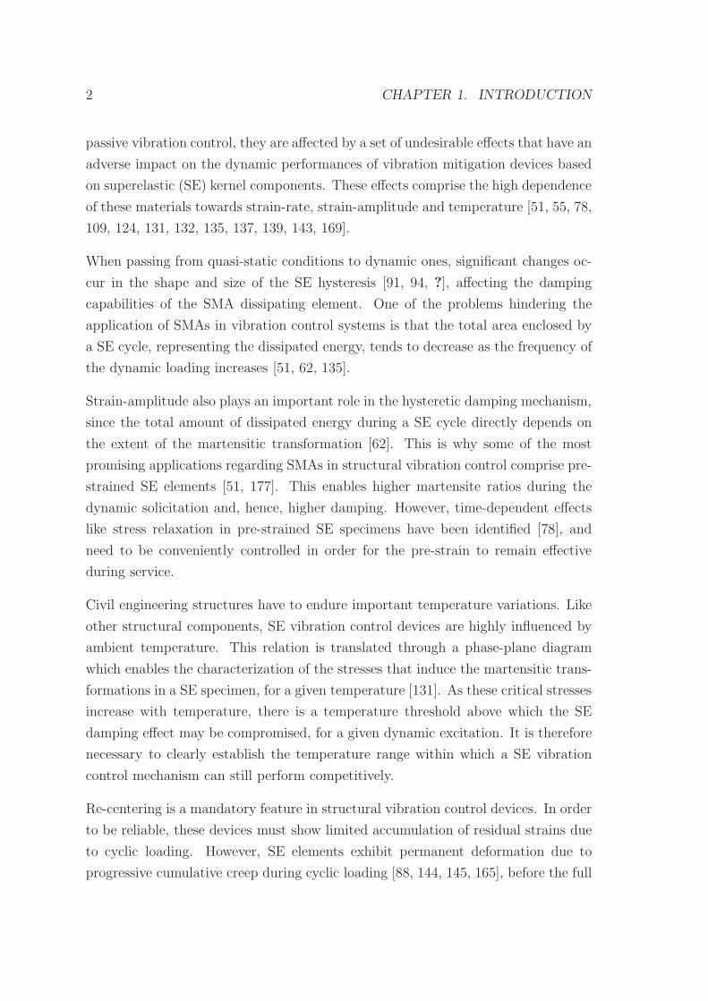
1.1 Problem Description
Shape-memory alloys (SMAs) are a unique class of metallic alloys that show two out-
standing properties: the shape-memory effect and superelasticity. These properties
derive from the ability of these materials to develop a diffusionless phase transfor-
mation in solids called martensitic transformation. The shape-memory effect allows
the material to recover its original geometry during heating, after being deformed.
Superelasticity enables the material to withstand large cyclic deformations, without
residual strains, while developing a hysteretic loop. The formation of this hysteretic
loop translates into the ability of the material to dissipate energy. Due to this high
inherent damping, combined with repeatable re-centering capabilities and relatively
high strength properties, SMAs have been progressively introduced in new techno-
logical applications related with energy dissipation in civil engineering structural
design.
For the time being, most of the applications regarding the use of SMAs in civil en-
gineering structures are linked with the seismic resistance enhancement of cultural
heritage structures [35, 43, 77]. However, several studies have already proved the
effectiveness of SMAs in a wide range of vibration control devices, i.e. bracing sys-
tems [27, 53, 103, 177], base isolation systems [42, 149, 174], bridge hinge restraining
systems [8, 46, 82, 127] and structural connections [117, 157].
Although these studies have clearly demonstrated the vast potential of SMAs in
1
2 CHAPTER 1. INTRODUCTION
passive vibration control, they are affected by a set of undesirable effects that have an
adverse impact on the dynamic performances of vibration mitigation devices based
on superelastic (SE) kernel components. These effects comprise the high dependence
of these materials towards strain-rate, strain-amplitude and temperature [51, 55, 78,
109, 124, 131, 132, 135, 137, 139, 143, 169].
When passing from quasi-static conditions to dynamic ones, significant changes oc-
cur in the shape and size of the SE hysteresis [91, 94, ?], affecting the damping
capabilities of the SMA dissipating element. One of the problems hindering the
application of SMAs in vibration control systems is that the total area enclosed by
a SE cycle, representing the dissipated energy, tends to decrease as the frequency of
the dynamic loading increases [51, 62, 135].
Strain-amplitude also plays an important role in the hysteretic damping mechanism,
since the total amount of dissipated energy during a SE cycle directly depends on
the extent of the martensitic transformation [62]. This is why some of the most
promising applications regarding SMAs in structural vibration control comprise pre-
strained SE elements [51, 177]. This enables higher martensite ratios during the
dynamic solicitation and, hence, higher damping. However, time-dependent effects
like stress relaxation in pre-strained SE specimens have been identified [78], and
need to be conveniently controlled in order for the pre-strain to remain effective
during service.
Civil engineering structures have to endure important temperature variations. Like
other structural components, SE vibration control devices are highly influenced by
ambient temperature. This relation is translated through a phase-plane diagram
which enables the characterization of the stresses that induce the martensitic trans-
formations in a SE specimen, for a given temperature [131]. As these critical stresses
increase with temperature, there is a temperature threshold above which the SE
damping effect may be compromised, for a given dynamic excitation. It is therefore
necessary to clearly establish the temperature range within which a SE vibration
control mechanism can still perform competitively.
Re-centering is a mandatory feature in structural vibration control devices. In order
to be reliable, these devices must show limited accumulation of residual strains due
to cyclic loading. However, SE elements exhibit permanent deformation due to
progressive cumulative creep during cyclic loading [88, 144, 145, 165], before the full
1.2. OBJECTIVES AND SCOPE 3
stabilization of the SE hysteresis. This causes the net strain produced by a given
structural oscillation to be reduced, decreasing the energy dissipation capabilities
of the material. This effect may be controlled by an initial training procedure,
or by limiting the stress levels during the dynamic loading within a narrower SE
window [107, 111].
These effects may constitute an important setback to the application of SMAs in
structural vibration control.
1.2 Objectives and Scope
The main objective of this dissertation is the material characterization of SE NiTi
while exploring the feasibility and optimal behavior of SMAs when used in structural
vibration control.
A set of parametric studies comprising experimental uniaxial tensile tests in SE
NiTi wires, with various strain-rates, strain-amplitudes and ambient temperatures
are performed, aiming to provide a valuable insight to the behavior of SMAs, and
assess their adequacy to seismic vibration control in civil engineering structures.
The cyclic behavior of NiTi wires is also investigated through an experimental ap-
proach, addressing the effects of cycling on cumulative creep, critical stress to induce
martensite and hysteretic width.
A numerical framework adequately describing the complex thermo-mechanical be-
havior of the SMAs is developed, taking into consideration the knowledge yielded
from the experimental program. This numerical framework is used to explore sev-
eral constitutive models and congurations for SMAs, using bibliographic referenced
models as a starting point for the research [15, 30, 60, 103, 159, 169]. The perfor-
mance of these models is evaluated in order to adopt a suitable numerical model
for fast dynamic SE simulations, also identifying the most significant SMA param-
eters affecting the dynamic response of a structural system. The numerical model
is then used in a seismic simulation of SE bridge restraining devices, one of the
most promising applications SMAs in civil engineering structures. The restrainers
are aimed to prevent unseating during earthquakes due to excessive relative hinge
opening and displacements [8, 46].
4 CHAPTER 1. INTRODUCTION
A control strategy aiming for the attenuation or suppression of the undesirable ef-
fects affecting SMAs, which have an adverse impact on their dynamic performances,
is developed. This control strategy is first implemented numerically to assess its
performance in structural vibration control. Once validated, the control strategy is
implemented in a small-scale prototype, reproducing a SE bridge restraining system.
This prototype is subjected to various dynamic actions including the ones produced
by a reduced shaking table.
1.3 Dissertation Outline
The content of the dissertation is organized into the following seven chapters:
Chapter 2 General introduction to SMAs, including a detailed description of the
martensitic transformation which is responsible for the superelasticity and
shape-memory effect in SMAs. Analysis of the SE energy dissipation mech-
anism and its application in vibration control devices. Bibliographic survey
regarding seismic hazard mitigation devices based in SE kernel elements.
Chapter 3 Analysis of the austenitic and martensitic crystallographic phases in
Nitinol. Description of an extensive experimental program regarding the char-
acterization of Nitinol, including temperature-controlled cyclic tensile tests,
differential scanning calorimetry and infrared thermo-imaging. Discussion of
the results obtained during the experimental procedures.
Chapter 4 Study of constitutive models for the mathematical modeling of SMAs
and corresponding governing laws, coupling the mechanical properties and
the transformation kinetics. Analysis of the convective heat transfer problem.
Numerical implementation and subsequent assessment and comparison of the
performance of the considered constitutive models.
Chapter 5 Numerical analysis of dynamic systems comprising SE components.
Study of three SDOF mechanisms based in SE restoring elements and evalua-
tion of their performance as passive vibration control systems. Application of
one of these devices in a simplified numerical model of a railway viaduct, as a
seismic restraining system and discussion of the obtained results.
1.3. DISSERTATION OUTLINE 5
Chapter 6 Numerical implementation of a semi-active control strategy aiming to
attenuate or suppress the undesirable effects affecting SMAs, which have an
adverse impact on their dynamic performances. Description of the proposed
vibration mitigation device and analysis of the results yielded by the numerical
tests.
Chapter 7 Analysis of a small-scale prototype for the simulation of a SE based
bridge restraining system. Description of the proportional-plus-integral-plus-
derivative (PID) algorithm used to control the mechanism. Discussion of the
experimental results.
Chapter 8 Summary of the research and conclusions. Discussion of the anticipated
impacts of the work and suggestions for future research.

6 CHAPTER 1. INTRODUCTION

Chapter 2
Shape-Memory Alloys in
Vibration Control Devices
2.1 Introduction
The emphasis which is currently given to energy dissipation in civil engineering struc-
tural design makes materials which are able to reduce vibrations increasingly more
appealing. The desired features of high strength, stiffness and tolerance to adverse
environments are, for most materials, incompatible with high damping capabilities.
Although viscoelastic materials are able to exhibit high damping capabilities, they
often show insufficient strength. In the last couple of years, a set of high damping
metallic alloys, combining high inherent damping with relatively high strength prop-
erties, have been progressively introduced in new technological applications. They
are called Shape-Memory Alloys . Two of their most important properties are the so
called shape-memory effect and superelasticity.
The shape-memory effect is a unique property of certain alloys that exhibit marten-
sitic transformations, that enables the material to recover its original shape, after
being deformed upon heating to a critical temperature. Superelasticity is associated
with large nonlinear recoverable strains (up to 8%) during a mechanical cycle of
loading and unloading [141]. Associated with the discovery of the superelasticity is
the Swedish physicist Arne Olander, in the year of 1932, when he first encountered
the SE behavior using an AuCd alloy [124]. In 1938, Greninger and Moorandian
7
8 CHAPTER 2. SMAS IN VIBRATION CONTROL DEVICES
observed the disappearance and reappearance of a martensitic crystal structure by
increasing and decreasing the temperature of a CuZn alloy [66]. The thermoelastic
properties of the martensitic crystal phase of an AuCd alloy were widely reported
by Kurdjumov and Khandros (1949) [86], and Chang and Read (1951) [37]. In the
1960s, Buehler and Wiley discovered the NiTi alloys, while working at the Naval
Ordnance Laboratory (NOL). The NOL, now disestablished, was formerly located
in White Oak, Maryland and was the site of considerable work that had practi-
cal impact upon world technology. As a tribute to their workplace, they named
this family of alloys Nitinol [71]. While the potential applications for Nitinol were
realized immediately, practical efforts to commercialize the alloy didn’t take place
until a decade later. This delay was largely due to the extraordinary difficulty in
melting, processing and machining the alloy, technological processes that weren’t
really overcome until the 1990s, when finally these practical difficulties began to be
resolved [71].
Shape-memory alloys and other types of smart materials (i.e. piezoelectric materials,
magnetorheologic fluids and so on) are being progressively introduced in lectures of
engineering courses. Also, in the last years, SMAs have been the object of various
innovative studies and industrial applications [8, 11, 25, 27, 42, 46, 53, 70, 82, 95,
97, 103, 112, 117, 125, 127, ?, 149, 157, 174, 177, 178].
2.2 General aspects of Shape-Memory alloys
2.2.1 Martensitic transformation
The transformation which yields superelasticity and the shape-memory effect is a
diffusionless phase transformation in solids, called martensitic transformation. Dur-
ing this transformation, the atoms are cooperatively rearranged into a different crys-
talline structure with identical chemical composition, through a displacive distortion
process [60]. The absence of diffusion, without the net transport of atoms, makes the
martensitic phase transformation almost instantaneous [131]. In SMAs, the marten-
sitic transformation changes the material from the parent phase, a high-temperature
(high-energy) phase called austenite, to a low-temperature phase (low-energy) called
martensite. Being a first-order phase transition, parent and product phases coexist
2.2. GENERAL ASPECTS OF SHAPE-MEMORY ALLOYS 9
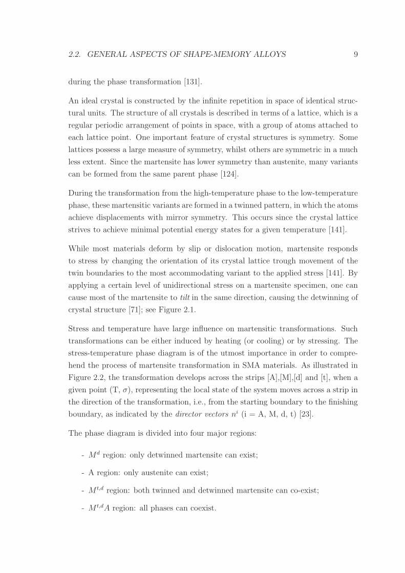
during the phase transformation [131].
An ideal crystal is constructed by the infinite repetition in space of identical struc-
tural units. The structure of all crystals is described in terms of a lattice, which is a
regular periodic arrangement of points in space, with a group of atoms attached to
each lattice point. One important feature of crystal structures is symmetry. Some
lattices possess a large measure of symmetry, whilst others are symmetric in a much
less extent. Since the martensite has lower symmetry than austenite, many variants
can be formed from the same parent phase [124].
During the transformation from the high-temperature phase to the low-temperature
phase, these martensitic variants are formed in a twinned pattern, in which the atoms
achieve displacements with mirror symmetry. This occurs since the crystal lattice
strives to achieve minimal potential energy states for a given temperature [141].
While most materials deform by slip or dislocation motion, martensite responds
to stress by changing the orientation of its crystal lattice trough movement of the
twin boundaries to the most accommodating variant to the applied stress [141]. By
applying a certain level of unidirectional stress on a martensite specimen, one can
cause most of the martensite to tilt in the same direction, causing the detwinning of
crystal structure [71]; see Figure 2.1.
Stress and temperature have large influence on martensitic transformations. Such
transformations can be either induced by heating (or cooling) or by stressing. The
stress-temperature phase diagram is of the utmost importance in order to compre-
hend the process of martensite transformation in SMA materials. As illustrated in
Figure 2.2, the transformation develops across the strips [A],[M],[d] and [t], when a
given point (T, σ), representing the local state of the system moves across a strip in
the direction of the transformation, i.e., from the starting boundary to the finishing
boundary, as indicated by the director vectors ni (i = A, M, d, t) [23].
The phase diagram is divided into four major regions:
- Md region: only detwinned martensite can exist;
- A region: only austenite can exist;
- M t,d region: both twinned and detwinned martensite can co-exist;
- M t,dA region: all phases can coexist.
10 CHAPTER 2. SMAS IN VIBRATION CONTROL DEVICES
Martensite(twinned)
detwinning
HeatingCooling
(parent phase)Austenite
Martensite(detwinned)
Deformation
Heating
Temperature
Figure 2.1: Schematic diagram of martensitic transformations (after Otsuka andWayman [124]).
AfAsMs
M t,d
Md
nd
nA
[M ]
[t]
nt
M t,dA
Mf
[d]
nM
[A]A
(T )
(σ)
Figure 2.2: Typical uniaxial stress-temperature phase diagram of SMA material.Transformation strips are the unshaded regions (after Bekker and Brinson [23]).
2.2. GENERAL ASPECTS OF SHAPE-MEMORY ALLOYS 11
In the stress-free state, a SMA is characterized by four transformation temperatures:
Ms andMf during cooling and As and Af during heating. The first two (withMs >
Mf ) indicate the temperatures at which the forward transformation starts and fin-
ishes, respectively. The last two (with As < Af) are the temperatures at which the
inverse transformation starts and finishes, Af being the temperature above which
the martensite becomes completely unstable [124]. Another important temperature
value is Md, which is an upper temperature limit above which martensite cannot
be stress-induced [55], because of the stability attained by austenite [109]. These
transformation temperatures depend mainly on the alloy’s composition and process-
ing [131].
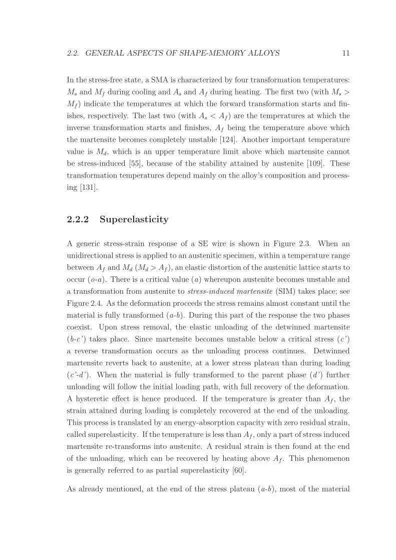
2.2.2 Superelasticity
A generic stress-strain response of a SE wire is shown in Figure 2.3. When an
unidirectional stress is applied to an austenitic specimen, within a temperature range
between Af andMd (Md > Af ), an elastic distortion of the austenitic lattice starts to
occur (o-a). There is a critical value (a) whereupon austenite becomes unstable and
a transformation from austenite to stress-induced martensite (SIM) takes place; see
Figure 2.4. As the deformation proceeds the stress remains almost constant until the
material is fully transformed (a-b). During this part of the response the two phases
coexist. Upon stress removal, the elastic unloading of the detwinned martensite
(b-c’ ) takes place. Since martensite becomes unstable below a critical stress (c’ )
a reverse transformation occurs as the unloading process continues. Detwinned
martensite reverts back to austenite, at a lower stress plateau than during loading
(c’-d’ ). When the material is fully transformed to the parent phase (d’ ) further
unloading will follow the initial loading path, with full recovery of the deformation.
A hysteretic effect is hence produced. If the temperature is greater than Af , the
strain attained during loading is completely recovered at the end of the unloading.
This process is translated by an energy-absorption capacity with zero residual strain,
called superelasticity. If the temperature is less thanAf , only a part of stress induced
martensite re-transforms into austenite. A residual strain is then found at the end
of the unloading, which can be recovered by heating above Af . This phenomenon
is generally referred to as partial superelasticity [60].
As already mentioned, at the end of the stress plateau (a-b), most of the material
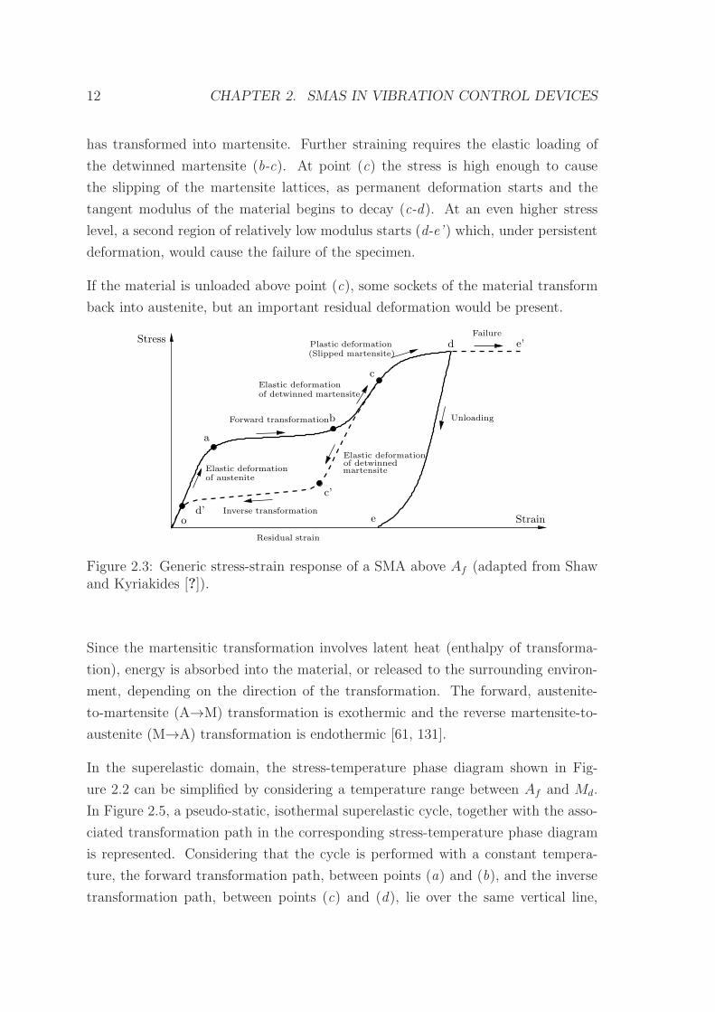
12 CHAPTER 2. SMAS IN VIBRATION CONTROL DEVICES
has transformed into martensite. Further straining requires the elastic loading of
the detwinned martensite (b-c). At point (c) the stress is high enough to cause
the slipping of the martensite lattices, as permanent deformation starts and the
tangent modulus of the material begins to decay (c-d). At an even higher stress
level, a second region of relatively low modulus starts (d-e’ ) which, under persistent
deformation, would cause the failure of the specimen.
If the material is unloaded above point (c), some sockets of the material transform
back into austenite, but an important residual deformation would be present.
of austeniteElastic deformation
Elastic deformation
martensiteof detwinned
(Slipped martensite)Plastic deformation
Elastic deformationof detwinned martensite
Forward transformation
c’
Stress
o
a
e’
Unloading
d
c
b
e Straind’ Inverse transformation
Residual strain
Failure
Figure 2.3: Generic stress-strain response of a SMA above Af (adapted from Shawand Kyriakides [?]).
Since the martensitic transformation involves latent heat (enthalpy of transforma-
tion), energy is absorbed into the material, or released to the surrounding environ-
ment, depending on the direction of the transformation. The forward, austenite-
to-martensite (A→M) transformation is exothermic and the reverse martensite-to-
austenite (M→A) transformation is endothermic [61, 131].
In the superelastic domain, the stress-temperature phase diagram shown in Fig-
ure 2.2 can be simplified by considering a temperature range between Af and Md.
In Figure 2.5, a pseudo-static, isothermal superelastic cycle, together with the asso-
ciated transformation path in the corresponding stress-temperature phase diagram
is represented. Considering that the cycle is performed with a constant tempera-
ture, the forward transformation path, between points (a) and (b), and the inverse
transformation path, between points (c) and (d), lie over the same vertical line,
2.2. GENERAL ASPECTS OF SHAPE-MEMORY ALLOYS 13
Martensite(detwinned)
exothermictransformation
endothermictransformation
Austenite(parent phase)
T > Af
Deformation
Figure 2.4: Mechanism of superelasticity (after Otsuka and Wayman [124]).
associated with T = T0.
o
b
c
d
aa
b
ε
σ
T
σ
T0
A
c
d[A]
[M ]
M t,dA
Ms
Mf
As
Af
MdCM
CM
CA
CA
Figure 2.5: Isothermal path on phase diagram and correspondent hysteresis.
To characterize the stress effect on the martensitic transformation, the Clausius-
Clapeyron relation is often used [124]. The Clausius-Clapeyron equation relates tem-
perature and stress along the transformation strips of the SMA stress-temperature
phase diagram. This relation, for uniaxial stress, may be written as follows,
dσ
dT= −
∆H
εT0(2.1)
where σ is the uniaxial stress, ε is the transformation strain and ∆H is the enthalpy
of the transformation per unit volume for temperature T0 [29].
During the forward transformation, which is exothermic, an overall decrease in en-
thalpy occurs, achieved by the generation of heat. In this case, ∆H is negative. On
14 CHAPTER 2. SMAS IN VIBRATION CONTROL DEVICES
the other hand, during the reverse transformation, which is endothermic, heat is
absorbed by the system and ∆H is positive.
The relation between temperature and the critical stress to induce the martensitic
transformation can be described by the material properties CM and CA. These
values represent the slope (dσ/dT ) of the lines defining the boundaries of the SMA
transformation strips, represented in Figure 2.5. Although experimental results for
the determination of critical stress values associated with the beginning and the end
of the forward and inverse transformations do rarely yield precisely linear results,
it is usual to admit that the relation between critical stress and temperature tends
to be approximately linear. It is generally assumed that both CM and CA have the
same value, constant over all temperature ranges [29]. This value is also referred to
as the Clausius-Clapeyron coefficient (CCC or αCC) [78].
2.2.3 Shape-Memory effect
The other manifestation of the thermoelastic martensitic transformation in SMAs
is the so called shape-memory effect. Whereas stressed induced martensite consists
of a single preferential variant according to the applied stress, martensite produced
by cooling consists of a random mixture of several variants (including twins). Twin
boundaries can be relatively easily moved by the application of stress. Movement
of twin boundaries by stressing, called detwinning, results in change of orientation
from one variant to another which is more favorably oriented to the direction of
the applied stress. During the detwinning process of the martensitic crystal struc-
ture, when facing an unidirectional loading, the stress remains almost constant until
the martensite is completely detwinned. Crystals favorably aligned to the load di-
rection deform first, at a lower stress level, (o-a-b) in Figure 2.6. Less favorably
aligned crystals deform later, at higher stresses (b-c). Further straining causes the
elastic loading of the detwinned martensite (c-d). Unloading from any point in (o-
d) initially results in elastic unloading of the detwinned material. The deformation
recovered is much smaller than the one supplied by detwinning, giving the apparent
impression of permanent deformation. This deformation can be recovered by raising
the temperature above Af , transforming the detwinned martensite back to austen-
ite; see Figure 2.7. This shape is maintained during cooling below Mf , when the
material re-transforms to twinned martensite. Straining further than point (d) will
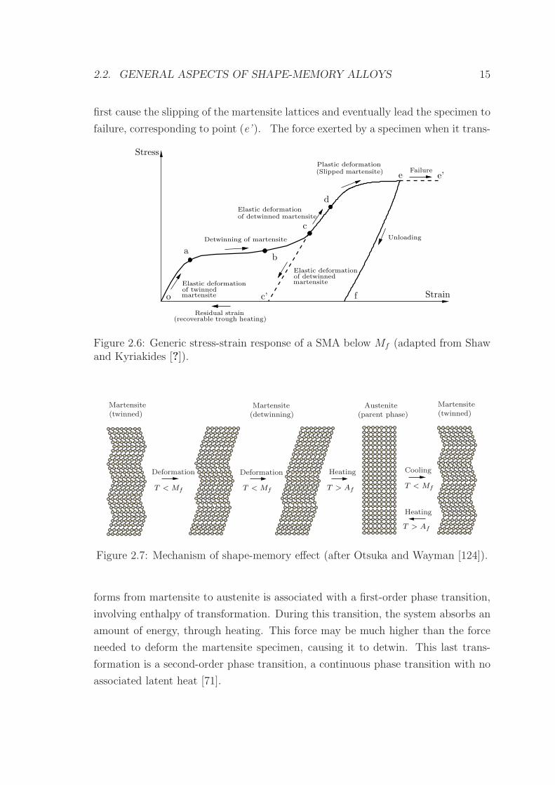
2.2. GENERAL ASPECTS OF SHAPE-MEMORY ALLOYS 15
first cause the slipping of the martensite lattices and eventually lead the specimen to
failure, corresponding to point (e’ ). The force exerted by a specimen when it trans-
Residual strain(recoverable trough heating)
Elastic deformation
martensiteof twinned
Plastic deformation(Slipped martensite)
Elastic deformation
martensiteof detwinned
Elastic deformationof detwinned martensite
o c’
a
Unloading
e’Failure
Stress
Strain
c
d
e
f
Detwinning of martensite
b
Figure 2.6: Generic stress-strain response of a SMA below Mf (adapted from Shawand Kyriakides [?]).
T < Mf T < Mf T > AfT < Mf
T > Af
Martensite(twinned)
Deformation
(detwinning)Martensite
Deformation Heating
Austenite(parent phase)
Martensite(twinned)
Cooling
Heating
Figure 2.7: Mechanism of shape-memory effect (after Otsuka and Wayman [124]).
forms from martensite to austenite is associated with a first-order phase transition,
involving enthalpy of transformation. During this transition, the system absorbs an
amount of energy, through heating. This force may be much higher than the force
needed to deform the martensite specimen, causing it to detwin. This last trans-
formation is a second-order phase transition, a continuous phase transition with no
associated latent heat [71].
16 CHAPTER 2. SMAS IN VIBRATION CONTROL DEVICES
Finally, a sequence of martensitic transformations is shown in Figure 2.8, combining
both a superelastic cycle and a shape-memory recovery.
Forward transformation
Inverse transformation
unloading withresidual strain
unloading withno residual strain
Strain
T = As
T = Af
T < Mf
SUPERELASTIC
SHAPE MEMORY
T > Af
Temperature
Strain
Stress
Stress
Detwinning
Figure 2.8: Shape-memory and superelastic sequence. Three dimensional stress,strain and temperature diagram.
2.2.4 Internal friction
The martensitic transformation involves latent heat, i.e. energy is absorbed into the
material or released to the surrounding environment, depending on the direction of
the transformation. The energy generated during one tensile cycle is proportional
to the volume fraction of formed martensite, reaching its maximum at the middle
of the solicitation.
The other source of energy generation during martensitic transformation is the in-
ternal friction. The amount of energy dissipated due to internal friction is always
small compared to the latent heat of transformation [122]. It is generally accepted
that internal friction, or damping capacity of SMAs, derives from the movement be-
tween martensite-martensite and parent-martensite transforming interfaces [124, ?].
2.2. GENERAL ASPECTS OF SHAPE-MEMORY ALLOYS 17
This energy loss due to interfacial motion enables a high degree of strain reversibil-
ity while providing material damping, in contrast to dislocation based plasticity, in
which damping is associated with irreversible inelastic deformations [?]. Internal
friction is usually related to the dissipative response of a material when subjected
to a cyclic deformation [90].
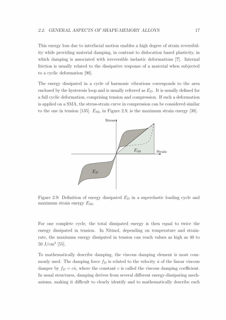
The energy dissipated in a cycle of harmonic vibrations corresponds to the area
enclosed by the hysteresis loop and is usually referred as ED. It is usually defined for
a full cyclic deformation, comprising tension and compression. If such a deformation
is applied on a SMA, the stress-strain curve in compression can be considered similar
to the one in tension [135]. ES0, in Figure 2.9, is the maximum strain energy [38].
Strain
Stress
ES0
ED
Figure 2.9: Definition of energy dissipated ED in a superelastic loading cycle andmaximum strain energy ES0.
For one complete cycle, the total dissipated energy is then equal to twice the
energy dissipated in tension. In Nitinol, depending on temperature and strain-
rate, the maximum energy dissipated in tension can reach values as high as 40 to
50 J/cm3 [55].
To mathematically describe damping, the viscous damping element is most com-
monly used. The damping force fD is related to the velocity u of the linear viscous
damper by fD = cu, where the constant c is called the viscous damping coefficient.
In usual structures, damping derives from several different energy-dissipating mech-
anisms, making it difficult to clearly identify and to mathematically describe each
18 CHAPTER 2. SMAS IN VIBRATION CONTROL DEVICES
one of these mechanisms. Therefore, the damping coefficient of a given structure
is chosen in such a way that the vibrational energy it dissipates equals the energy
dissipated in all of the combined damping mechanisms present in the structure. This
idealization is called equivalent viscous damping [38].
The most common method for defining the equivalent viscous damping is to equate
the energy dissipated in a vibration cycle of the actual structure and an equivalent
viscous system. The equivalent viscous damping as a measure of damping or internal
friction in a structure is very advantageous since it is clearly defined in terms of
observable quantities. For a given dynamic system, the stress-strain relation can be
easily obtained through a cyclic loading experiment. The subsequent evaluation of
the area enclosed by the hysteresis, corresponding to the dissipated energy (ED), is
very simple to compute.
The energy dissipated by a viscous system is given by
ED =
∫
fD du (2.2)
where fD is the damping force. The steady-state vibrations of a single-degree-
of-freedom (SDOF) system due to an harmonic force can be described as u(t) =
u0sin(ωt− φ). The dissipated energy in one cycle of harmonic vibration equals
ED =
∫ 2π/ω
0
(cu)u dt = πcωu02 (2.3)
As the damping ratio, ζ is defined by
ζ =c
2mωn(2.4)
and the natural undamped frequency of the system is defined by ωn =√
k/m,
expression (2.3) may be rewritten as
ED = 2πζω
ωnku0
2 (2.5)
Taking into account that the maximum strain energy is ES0 = ku02/2, equation (2.5)
2.3. VIBRATION CONTROL DEVICES 19
can be rewritten as
ED = 4πζω
ωnES0 (2.6)
or
ζ =1
4π
ωn
ω
ED
ES0(2.7)
If the stress-strain hysteresis, and the correspondent ED, is determined at ω = ωn,
equation (2.7) specializes to
ζeq =1
4π
ED
ES0(2.8)
The damping ratio ζeq determined with ω = ωn would not be correct at any other
exciting frequency, but it would be a satisfactory approximation [38].
2.3 Vibration control devices
Technological applications built up of shape-memory components are designed to
take advantage of the shape-memory effect and/or superelasticity. Regarding the
shape-memory effect, three different categories are usually considered for the afore-
mentioned applications, i.e., free recovery, constrained recovery and actuators [55].
Free recovery is when a shape-memory component is allowed to freely recover its
original shape during heating, generating a recovery strain. If this recovery is pre-
vented, constraining the material in its martensitic form while recovering, large
stresses are developed, although no strain is recovered. These applications, based
on a constrained recovery, include fasteners and pipe couplings and are the oldest
and most widespread type of practical use [55]. In applications where there is both
a recovered strain and stress during heating, such as in the case of a Nitinol spring
being warmed to lift a ball, work is being done. Such applications are often further
categorized according to their actuation mode, i.e. electrical or thermal.
Technological applications based on SE components are mainly built for passive
energy dissipation. Like all passive control systems, these applications do not require
external power sources. Contrary to active control devices, which apply forces to the
structure in a prescribed manner, by means of an external power source, they impart
forces that are developed in response to the motion of the structure itself. When
a system combines the use o both active and passive control it is called a hybrid

20 CHAPTER 2. SMAS IN VIBRATION CONTROL DEVICES
control system. In a semi-active control system, mechanical energy is not added
into the structural system nor to the control actuators. These devices are mostly
passive control devices with controllable properties, and therefore have external
energy requirements which are orders of magnitude smaller than ordinary active
control systems [73].
Passive energy dissipation in a vibrating structure mainly occurs due to internal
stressing, rubbing, cracking, and plastic deformations [73]. When facing a dynamic
event, the amplitude of the structural vibrations varies inversely with the capacity
of the structure to dissipate energy. As some structures show very low damping,
they may experience large amplitudes of vibration even for moderately strong earth-
quakes. Increasing the energy dissipation capacity of a structure is a very effective
method to reduce the amplitudes of vibration. A great variety of different devices
providing supplemental damping exist and have been already installed in structures
all over the world, enhancing their energy dissipation capacity by converting kinetic
energy into heat. These devices operate on principles such as frictional sliding, defor-
mation of viscoelastic solids or fluids, yielding of metals and phase transformations
in metals or alloys. The latter method includes SE, which allows the material to
dissipate a considerable amount of energy through hysteresis, while recovering from
large nonlinear strains [73].
2.4 Seismic mitigation devices based on SMAs
Recent earthquakes in urban areas such as the Loma Prieta (1989) and the Northridge
(1994) earthquakes, in the U.S.A., the Kobe (1995) earthquake, in Japan, the Ko-
caeli (1999) earthquake, in Turkey, and the Nisqually (2001) earthquake, in the
U.S.A, resulted in significant damage to the civil engineering infrastructure [104].
Structural components suffered large permanent deformations as a result of conven-
tional design techniques, which rely on their inelastic response to dissipate energy
during a seismic event. As a result of these shortcomings, the structural engi-
neering community has concentrated on a performance-based design approach, to
earthquake mitigation in structures. The performance guidelines for such a design
approach mostly rely on the characterization of acceptable structural inter-story
drift values, for a given seismic hazard, where an increased maximum inter-story
2.4. SEISMIC MITIGATION DEVICES BASED ON SMAS 21
drift can be associated with increased damage levels [68].
Meanwhile, several devices aimed to limit the inelastic behavior of critical structural
members are being developed, in order to comply with these performance guidelines.
These devices are based on three primary concepts: energy dissipation (damping),
decoupling of the structure from the foundation (base isolation) and limiting the
force transmission to critical load bearing members [168].
The current development of both passive and active vibration control devices based
on these concepts has led to a recent interest in the use of smart materials. A
relatively consensual definition of a smart material is proposed in [106]: a struc-
tural material that inherently contains actuating, sensing and controlling capabili-
ties built into its microstructure. These materials undergo changes in one or more of
their properties (chemical, mechanical, electrical, magnetic or thermal) in a direct
response to an external stimuli associated with the environment surrounding the
material. These changes are direct and reversible, with no need for an external con-
trol system [1]. SMAs are one class of smart materials that have shown significant
potential for exploitation as a cost-effective mean to control the response of civil
engineering structures in both new and retrofit applications [49, 104].
2.4.1 Bracing systems
Most of the structural damages occurring in building structures during an earth-
quake event, result from large inter-story drifts. The addition of passive energy
dissipation bracing systems, connecting two consecutive storeys of the building,
have been proved effective in limiting such inter-story drifts, preventing significant
inelastic deformations in structural members [53].
Currently used bracing systems dissipate energy through yielding of metals, sliding
friction between suitable surfaces, motion of a piston or plate within viscous fluid, ex-
trusion of fluid through orifices or, finally, viscoelastic action of polymers. Recently,
SMAs are being increasingly considered for bracing systems in structures, in order
to limit inter-story and residual drifts, by providing additional energy dissipation
capacities and re-centering capabilities [53].
The use of SMAs in structural bracing systems has been addressed by several re-
searchers [2, 3, 14, 27, 34, 69, 99, 103, 110, 142, 158]. Some of these papers report
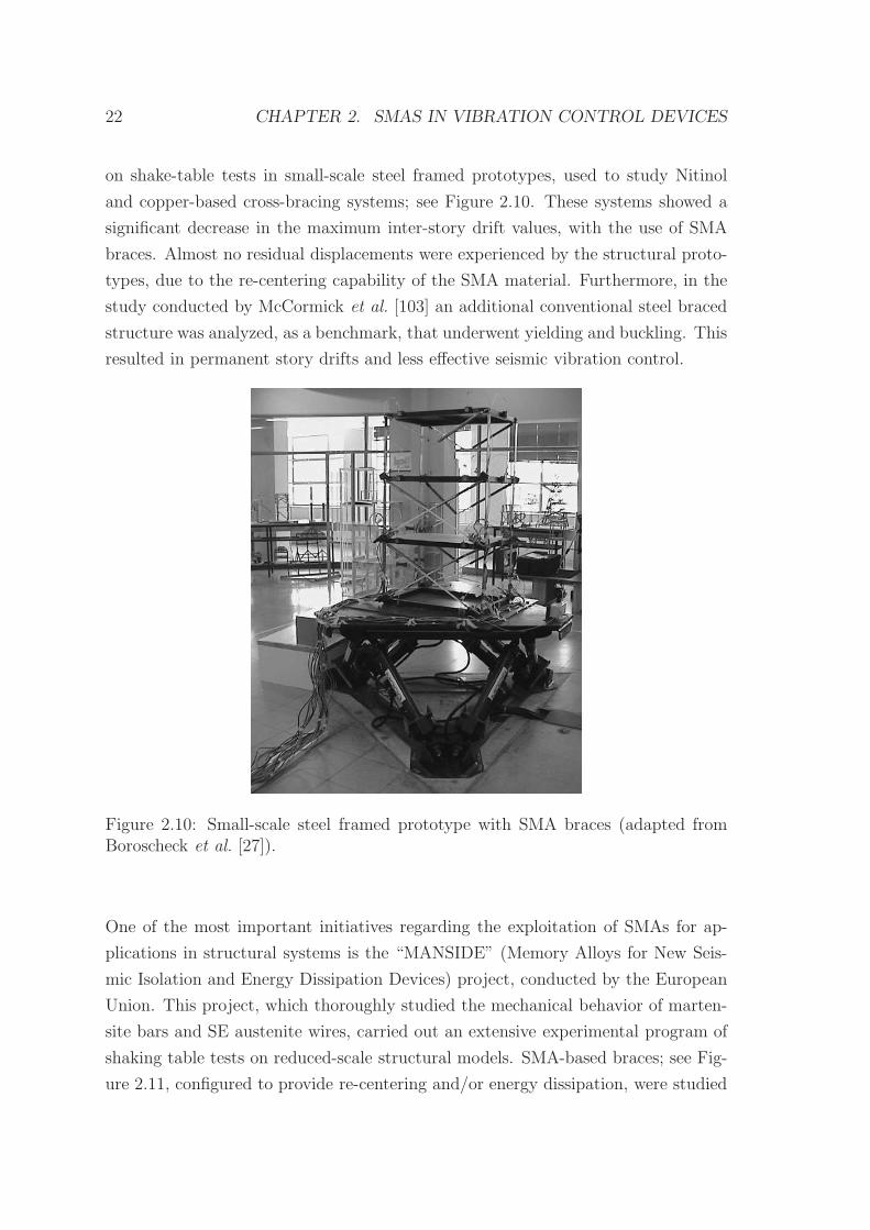
22 CHAPTER 2. SMAS IN VIBRATION CONTROL DEVICES
on shake-table tests in small-scale steel framed prototypes, used to study Nitinol
and copper-based cross-bracing systems; see Figure 2.10. These systems showed a
significant decrease in the maximum inter-story drift values, with the use of SMA
braces. Almost no residual displacements were experienced by the structural proto-
types, due to the re-centering capability of the SMA material. Furthermore, in the
study conducted by McCormick et al. [103] an additional conventional steel braced
structure was analyzed, as a benchmark, that underwent yielding and buckling. This
resulted in permanent story drifts and less effective seismic vibration control.
Figure 2.10: Small-scale steel framed prototype with SMA braces (adapted fromBoroscheck et al. [27]).
One of the most important initiatives regarding the exploitation of SMAs for ap-
plications in structural systems is the “MANSIDE” (Memory Alloys for New Seis-
mic Isolation and Energy Dissipation Devices) project, conducted by the European
Union. This project, which thoroughly studied the mechanical behavior of marten-
site bars and SE austenite wires, carried out an extensive experimental program of
shaking table tests on reduced-scale structural models. SMA-based braces; see Fig-
ure 2.11, configured to provide re-centering and/or energy dissipation, were studied
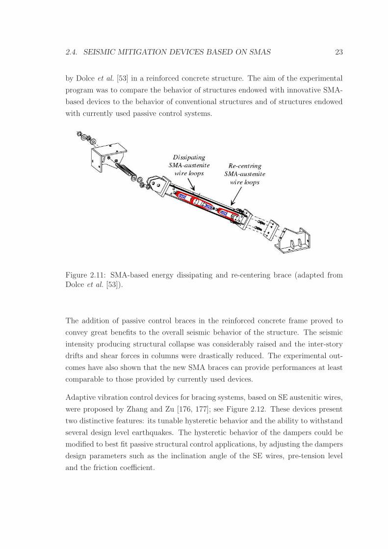
2.4. SEISMIC MITIGATION DEVICES BASED ON SMAS 23
by Dolce et al. [53] in a reinforced concrete structure. The aim of the experimental
program was to compare the behavior of structures endowed with innovative SMA-
based devices to the behavior of conventional structures and of structures endowed
with currently used passive control systems.
Figure 2.11: SMA-based energy dissipating and re-centering brace (adapted fromDolce et al. [53]).
The addition of passive control braces in the reinforced concrete frame proved to
convey great benefits to the overall seismic behavior of the structure. The seismic
intensity producing structural collapse was considerably raised and the inter-story
drifts and shear forces in columns were drastically reduced. The experimental out-
comes have also shown that the new SMA braces can provide performances at least
comparable to those provided by currently used devices.
Adaptive vibration control devices for bracing systems, based on SE austenitic wires,
were proposed by Zhang and Zu [176, 177]; see Figure 2.12. These devices present
two distinctive features: its tunable hysteretic behavior and the ability to withstand
several design level earthquakes. The hysteretic behavior of the dampers could be
modified to best fit passive structural control applications, by adjusting the dampers
design parameters such as the inclination angle of the SE wires, pre-tension level
and the friction coefficient.
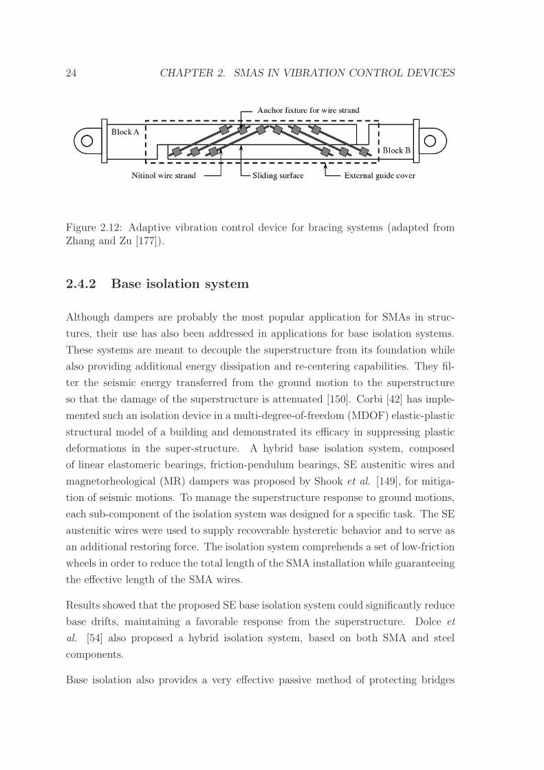
24 CHAPTER 2. SMAS IN VIBRATION CONTROL DEVICES
Figure 2.12: Adaptive vibration control device for bracing systems (adapted fromZhang and Zu [177]).
2.4.2 Base isolation system
Although dampers are probably the most popular application for SMAs in struc-
tures, their use has also been addressed in applications for base isolation systems.
These systems are meant to decouple the superstructure from its foundation while
also providing additional energy dissipation and re-centering capabilities. They fil-
ter the seismic energy transferred from the ground motion to the superstructure
so that the damage of the superstructure is attenuated [150]. Corbi [42] has imple-
mented such an isolation device in a multi-degree-of-freedom (MDOF) elastic-plastic
structural model of a building and demonstrated its efficacy in suppressing plastic
deformations in the super-structure. A hybrid base isolation system, composed
of linear elastomeric bearings, friction-pendulum bearings, SE austenitic wires and
magnetorheological (MR) dampers was proposed by Shook et al. [149], for mitiga-
tion of seismic motions. To manage the superstructure response to ground motions,
each sub-component of the isolation system was designed for a specific task. The SE
austenitic wires were used to supply recoverable hysteretic behavior and to serve as
an additional restoring force. The isolation system comprehends a set of low-friction
wheels in order to reduce the total length of the SMA installation while guaranteeing
the effective length of the SMA wires.
Results showed that the proposed SE base isolation system could significantly reduce
base drifts, maintaining a favorable response from the superstructure. Dolce et
al. [54] also proposed a hybrid isolation system, based on both SMA and steel
components.
Base isolation also provides a very effective passive method of protecting bridges
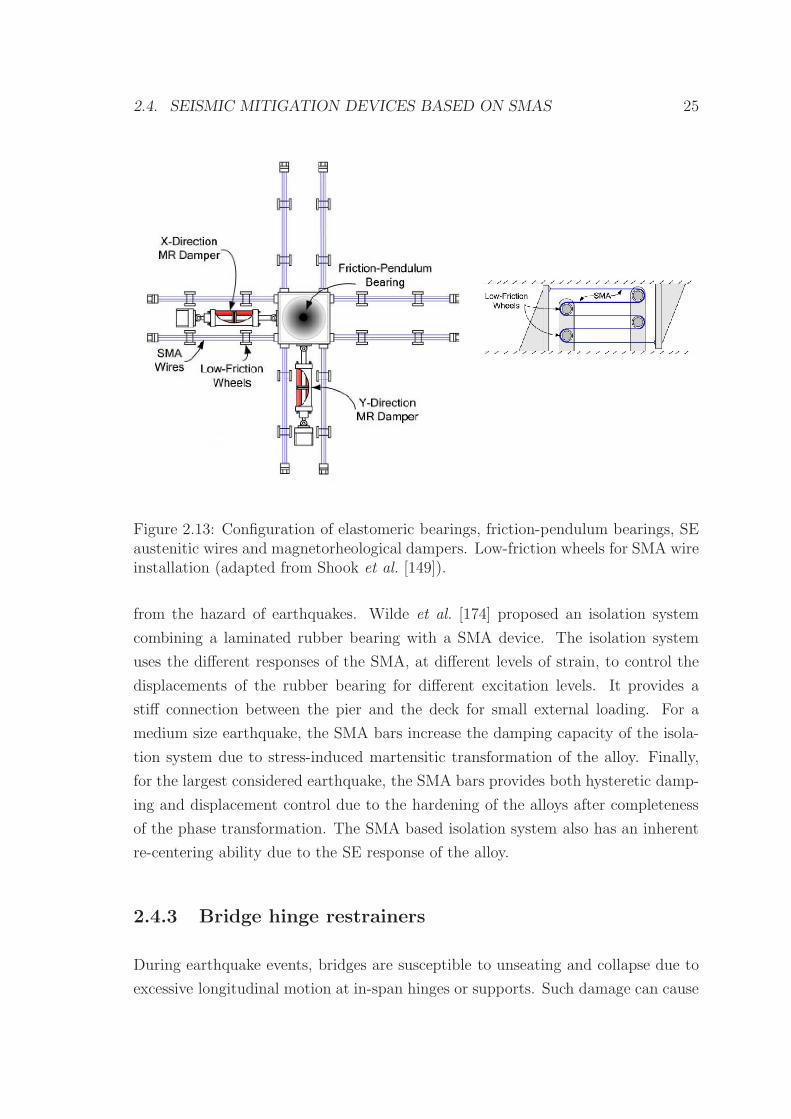
2.4. SEISMIC MITIGATION DEVICES BASED ON SMAS 25
Figure 2.13: Configuration of elastomeric bearings, friction-pendulum bearings, SEaustenitic wires and magnetorheological dampers. Low-friction wheels for SMA wireinstallation (adapted from Shook et al. [149]).
from the hazard of earthquakes. Wilde et al. [174] proposed an isolation system
combining a laminated rubber bearing with a SMA device. The isolation system
uses the different responses of the SMA, at different levels of strain, to control the
displacements of the rubber bearing for different excitation levels. It provides a
stiff connection between the pier and the deck for small external loading. For a
medium size earthquake, the SMA bars increase the damping capacity of the isola-
tion system due to stress-induced martensitic transformation of the alloy. Finally,
for the largest considered earthquake, the SMA bars provides both hysteretic damp-
ing and displacement control due to the hardening of the alloys after completeness
of the phase transformation. The SMA based isolation system also has an inherent
re-centering ability due to the SE response of the alloy.
2.4.3 Bridge hinge restrainers
During earthquake events, bridges are susceptible to unseating and collapse due to
excessive longitudinal motion at in-span hinges or supports. Such damage can cause
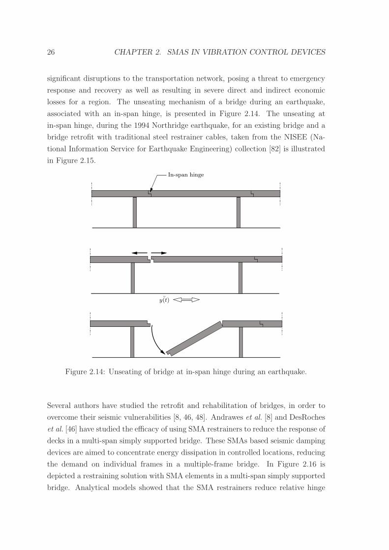
26 CHAPTER 2. SMAS IN VIBRATION CONTROL DEVICES
significant disruptions to the transportation network, posing a threat to emergency
response and recovery as well as resulting in severe direct and indirect economic
losses for a region. The unseating mechanism of a bridge during an earthquake,
associated with an in-span hinge, is presented in Figure 2.14. The unseating at
in-span hinge, during the 1994 Northridge earthquake, for an existing bridge and a
bridge retrofit with traditional steel restrainer cables, taken from the NISEE (Na-
tional Information Service for Earthquake Engineering) collection [82] is illustrated
in Figure 2.15.
¨y(t)
In-span hinge
Figure 2.14: Unseating of bridge at in-span hinge during an earthquake.
Several authors have studied the retrofit and rehabilitation of bridges, in order to
overcome their seismic vulnerabilities [8, 46, 48]. Andrawes et al. [8] and DesRoches
et al. [46] have studied the efficacy of using SMA restrainers to reduce the response of
decks in a multi-span simply supported bridge. These SMAs based seismic damping
devices are aimed to concentrate energy dissipation in controlled locations, reducing
the demand on individual frames in a multiple-frame bridge. In Figure 2.16 is
depicted a restraining solution with SMA elements in a multi-span simply supported
bridge. Analytical models showed that the SMA restrainers reduce relative hinge
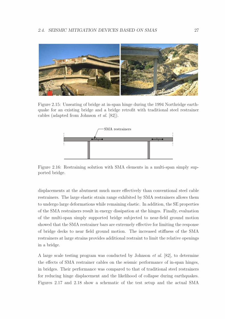
2.4. SEISMIC MITIGATION DEVICES BASED ON SMAS 27
Figure 2.15: Unseating of bridge at in-span hinge during the 1994 Northridge earth-quake for an existing bridge and a bridge retrofit with traditional steel restrainercables (adapted from Johnson et al. [82]).
SMA restrainers
Figure 2.16: Restraining solution with SMA elements in a multi-span simply sup-ported bridge.
displacements at the abutment much more effectively than conventional steel cable
restrainers. The large elastic strain range exhibited by SMA restrainers allows them
to undergo large deformations while remaining elastic. In addition, the SE properties
of the SMA restrainers result in energy dissipation at the hinges. Finally, evaluation
of the multi-span simply supported bridge subjected to near-field ground motion
showed that the SMA restrainer bars are extremely effective for limiting the response
of bridge decks to near field ground motion. The increased stiffness of the SMA
restrainers at large strains provides additional restraint to limit the relative openings
in a bridge.
A large scale testing program was conducted by Johnson et al. [82], to determine
the effects of SMA restrainer cables on the seismic performance of in-span hinges,
in bridges. Their performance was compared to that of traditional steel restrainers
for reducing hinge displacement and the likelihood of collapse during earthquakes.
Figures 2.17 and 2.18 show a schematic of the test setup and the actual SMA
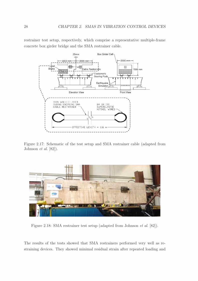
28 CHAPTER 2. SMAS IN VIBRATION CONTROL DEVICES
restrainer test setup, respectively, which comprise a representative multiple-frame
concrete box girder bridge and the SMA restrainer cable.
Figure 2.17: Schematic of the test setup and SMA restrainer cable (adapted fromJohnson et al. [82]).
Figure 2.18: SMA restrainer test setup (adapted from Johnson et al. [82]).
The results of the tests showed that SMA restrainers performed very well as re-
straining devices. They showed minimal residual strain after repeated loading and
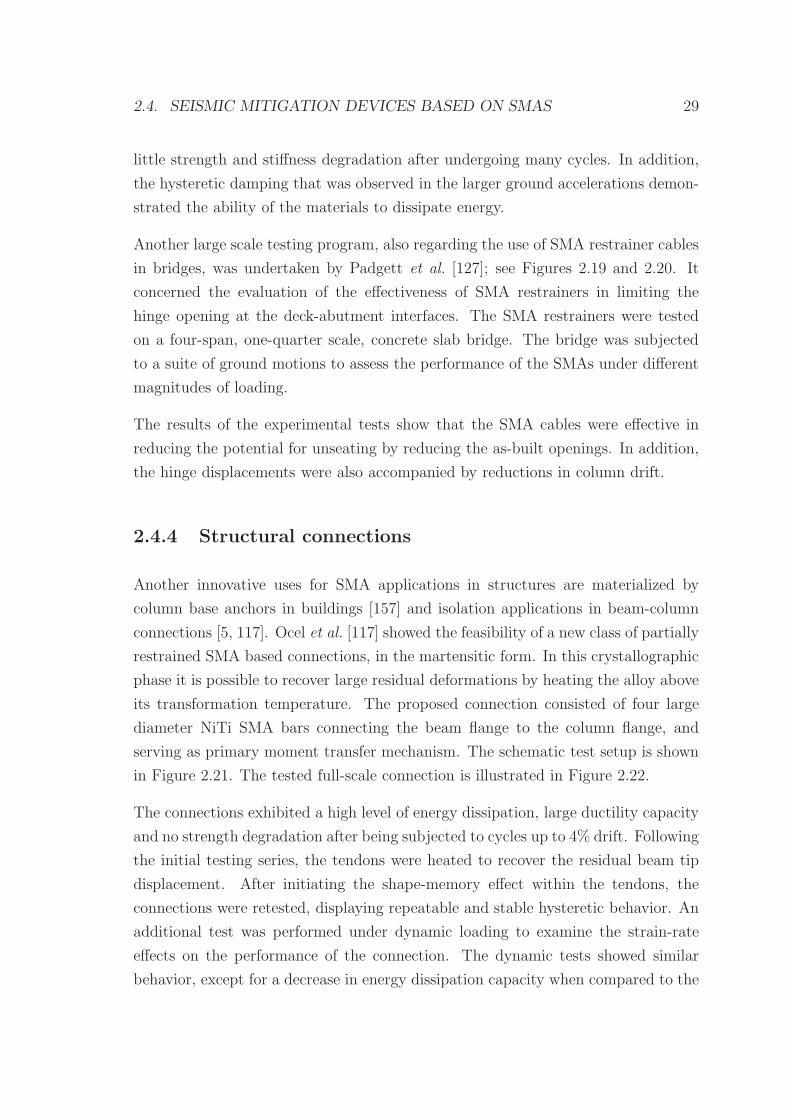
2.4. SEISMIC MITIGATION DEVICES BASED ON SMAS 29
little strength and stiffness degradation after undergoing many cycles. In addition,
the hysteretic damping that was observed in the larger ground accelerations demon-
strated the ability of the materials to dissipate energy.
Another large scale testing program, also regarding the use of SMA restrainer cables
in bridges, was undertaken by Padgett et al. [127]; see Figures 2.19 and 2.20. It
concerned the evaluation of the effectiveness of SMA restrainers in limiting the
hinge opening at the deck-abutment interfaces. The SMA restrainers were tested
on a four-span, one-quarter scale, concrete slab bridge. The bridge was subjected
to a suite of ground motions to assess the performance of the SMAs under different
magnitudes of loading.
The results of the experimental tests show that the SMA cables were effective in
reducing the potential for unseating by reducing the as-built openings. In addition,
the hinge displacements were also accompanied by reductions in column drift.
2.4.4 Structural connections
Another innovative uses for SMA applications in structures are materialized by
column base anchors in buildings [157] and isolation applications in beam-column
connections [5, 117]. Ocel et al. [117] showed the feasibility of a new class of partially
restrained SMA based connections, in the martensitic form. In this crystallographic
phase it is possible to recover large residual deformations by heating the alloy above
its transformation temperature. The proposed connection consisted of four large
diameter NiTi SMA bars connecting the beam flange to the column flange, and
serving as primary moment transfer mechanism. The schematic test setup is shown
in Figure 2.21. The tested full-scale connection is illustrated in Figure 2.22.
The connections exhibited a high level of energy dissipation, large ductility capacity
and no strength degradation after being subjected to cycles up to 4% drift. Following
the initial testing series, the tendons were heated to recover the residual beam tip
displacement. After initiating the shape-memory effect within the tendons, the
connections were retested, displaying repeatable and stable hysteretic behavior. An
additional test was performed under dynamic loading to examine the strain-rate
effects on the performance of the connection. The dynamic tests showed similar
behavior, except for a decrease in energy dissipation capacity when compared to the
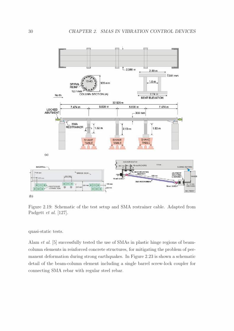
30 CHAPTER 2. SMAS IN VIBRATION CONTROL DEVICES
Figure 2.19: Schematic of the test setup and SMA restrainer cable. Adapted fromPadgett et al. [127].
quasi-static tests.
Alam et al. [5] successfully tested the use of SMAs in plastic hinge regions of beam-
column elements in reinforced concrete structures, for mitigating the problem of per-
manent deformation during strong earthquakes. In Figure 2.23 is shown a schematic
detail of the beam-column element including a single barrel screw-lock coupler for
connecting SMA rebar with regular steel rebar.
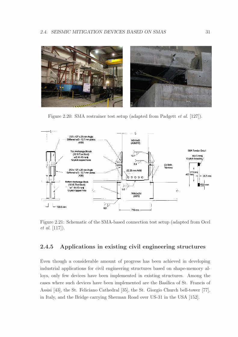
2.4. SEISMIC MITIGATION DEVICES BASED ON SMAS 31
Figure 2.20: SMA restrainer test setup (adapted from Padgett et al. [127]).
Figure 2.21: Schematic of the SMA-based connection test setup (adapted from Ocelet al. [117]).
2.4.5 Applications in existing civil engineering structures
Even though a considerable amount of progress has been achieved in developing
industrial applications for civil engineering structures based on shape-memory al-
loys, only few devices have been implemented in existing structures. Among the
cases where such devices have been implemented are the Basilica of St. Francis of
Assisi [43], the St. Feliciano Cathedral [35], the St. Giorgio Church bell-tower [77],
in Italy, and the Bridge carrying Sherman Road over US-31 in the USA [152].
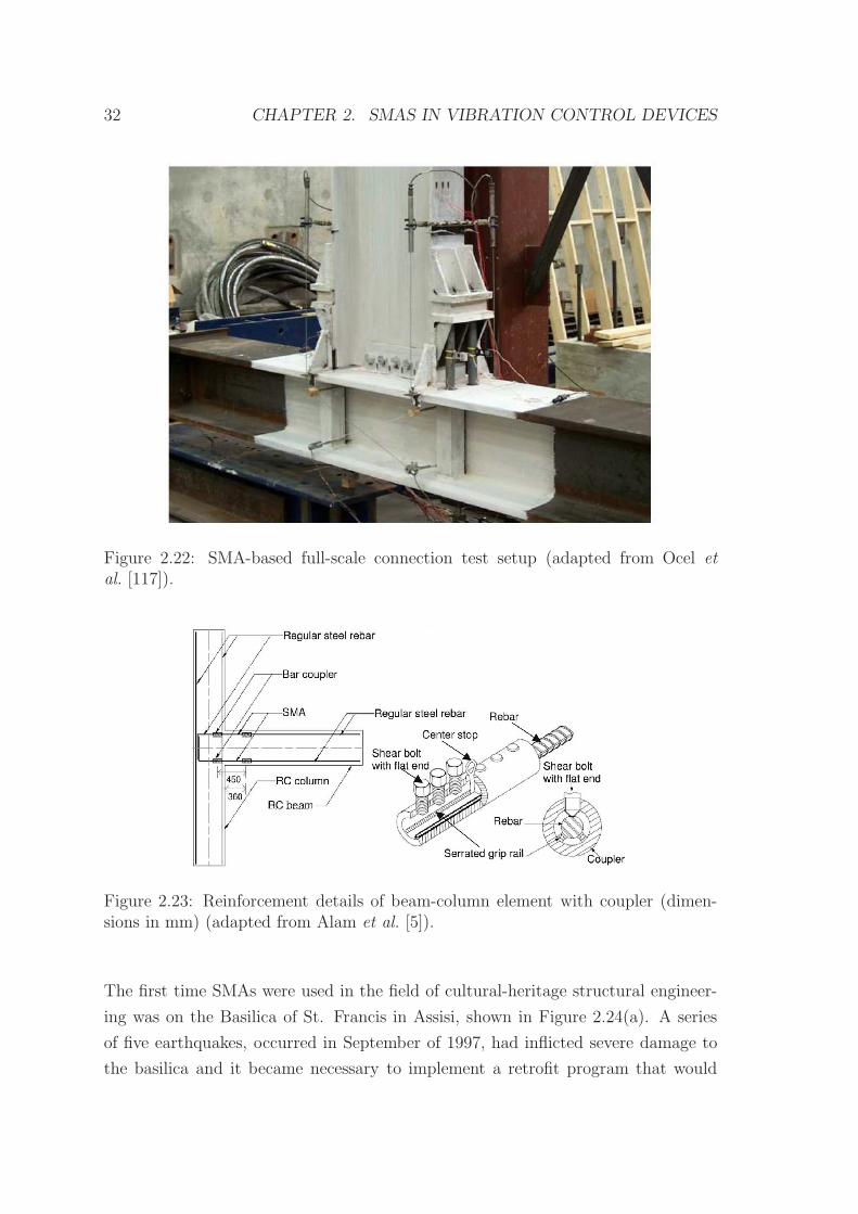
32 CHAPTER 2. SMAS IN VIBRATION CONTROL DEVICES
Figure 2.22: SMA-based full-scale connection test setup (adapted from Ocel etal. [117]).
Figure 2.23: Reinforcement details of beam-column element with coupler (dimen-sions in mm) (adapted from Alam et al. [5]).
The first time SMAs were used in the field of cultural-heritage structural engineer-
ing was on the Basilica of St. Francis in Assisi, shown in Figure 2.24(a). A series
of five earthquakes, occurred in September of 1997, had inflicted severe damage to
the basilica and it became necessary to implement a retrofit program that would
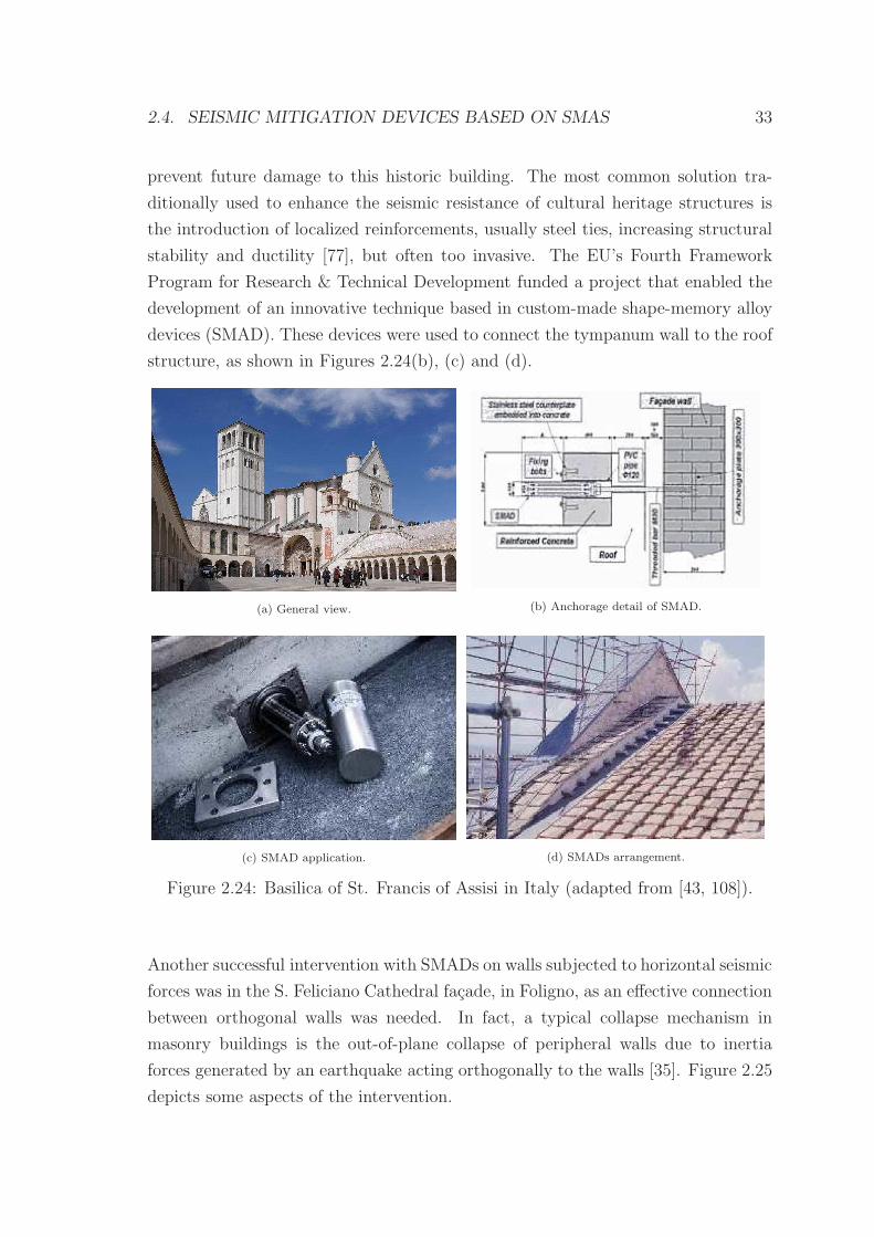
2.4. SEISMIC MITIGATION DEVICES BASED ON SMAS 33
prevent future damage to this historic building. The most common solution tra-
ditionally used to enhance the seismic resistance of cultural heritage structures is
the introduction of localized reinforcements, usually steel ties, increasing structural
stability and ductility [77], but often too invasive. The EU’s Fourth Framework
Program for Research & Technical Development funded a project that enabled the
development of an innovative technique based in custom-made shape-memory alloy
devices (SMAD). These devices were used to connect the tympanum wall to the roof
structure, as shown in Figures 2.24(b), (c) and (d).
(a) General view. (b) Anchorage detail of SMAD.
(c) SMAD application. (d) SMADs arrangement.
Figure 2.24: Basilica of St. Francis of Assisi in Italy (adapted from [43, 108]).
Another successful intervention with SMADs on walls subjected to horizontal seismic
forces was in the S. Feliciano Cathedral facade, in Foligno, as an effective connection
between orthogonal walls was needed. In fact, a typical collapse mechanism in
masonry buildings is the out-of-plane collapse of peripheral walls due to inertia
forces generated by an earthquake acting orthogonally to the walls [35]. Figure 2.25
depicts some aspects of the intervention.
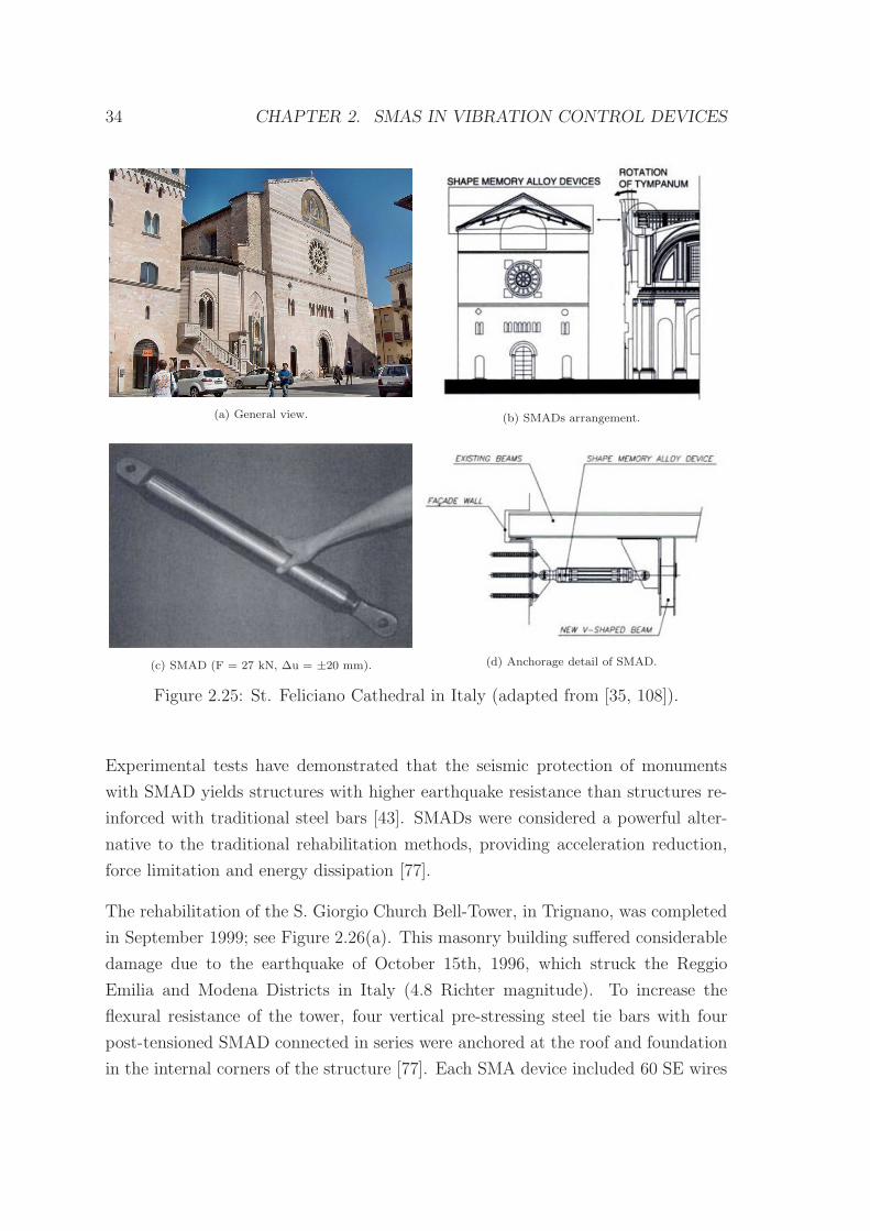
34 CHAPTER 2. SMAS IN VIBRATION CONTROL DEVICES
(a) General view. (b) SMADs arrangement.
(c) SMAD (F = 27 kN, ∆u = ±20 mm). (d) Anchorage detail of SMAD.
Figure 2.25: St. Feliciano Cathedral in Italy (adapted from [35, 108]).
Experimental tests have demonstrated that the seismic protection of monuments
with SMAD yields structures with higher earthquake resistance than structures re-
inforced with traditional steel bars [43]. SMADs were considered a powerful alter-
native to the traditional rehabilitation methods, providing acceleration reduction,
force limitation and energy dissipation [77].
The rehabilitation of the S. Giorgio Church Bell-Tower, in Trignano, was completed
in September 1999; see Figure 2.26(a). This masonry building suffered considerable
damage due to the earthquake of October 15th, 1996, which struck the Reggio
Emilia and Modena Districts in Italy (4.8 Richter magnitude). To increase the
flexural resistance of the tower, four vertical pre-stressing steel tie bars with four
post-tensioned SMAD connected in series were anchored at the roof and foundation
in the internal corners of the structure [77]. Each SMA device included 60 SE wires
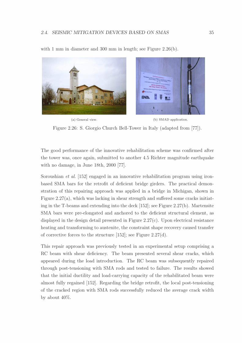
2.4. SEISMIC MITIGATION DEVICES BASED ON SMAS 35
with 1 mm in diameter and 300 mm in length; see Figure 2.26(b).
(a) General view. (b) SMAD application.
Figure 2.26: S. Giorgio Church Bell-Tower in Italy (adapted from [77]).
The good performance of the innovative rehabilitation scheme was confirmed after
the tower was, once again, submitted to another 4.5 Richter magnitude earthquake
with no damage, in June 18th, 2000 [77].
Soroushian et al. [152] engaged in an innovative rehabilitation program using iron-
based SMA bars for the retrofit of deficient bridge girders. The practical demon-
stration of this repairing approach was applied in a bridge in Michigan, shown in
Figure 2.27(a), which was lacking in shear strength and suffered some cracks initiat-
ing in the T-beams and extending into the deck [152]; see Figure 2.27(b). Martensite
SMA bars were pre-elongated and anchored to the deficient structural element, as
displayed in the design detail presented in Figure 2.27(c). Upon electrical resistance
heating and transforming to austenite, the constraint shape recovery caused transfer
of corrective forces to the structure [152]; see Figure 2.27(d).
This repair approach was previously tested in an experimental setup comprising a
RC beam with shear deficiency. The beam presented several shear cracks, which
appeared during the load introduction. The RC beam was subsequently repaired
through post-tensioning with SMA rods and tested to failure. The results showed
that the initial ductility and load-carrying capacity of the rehabilitated beam were
almost fully regained [152]. Regarding the bridge retrofit, the local post-tensioning
of the cracked region with SMA rods successfully reduced the average crack width
by about 40%.
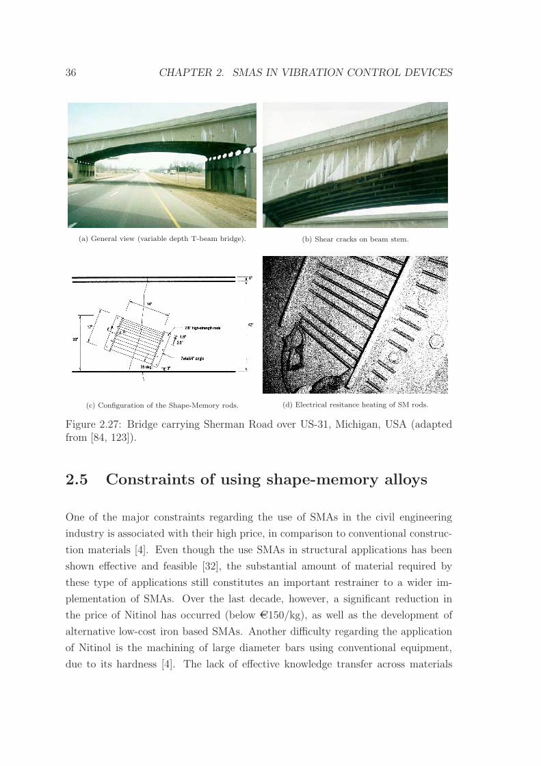
36 CHAPTER 2. SMAS IN VIBRATION CONTROL DEVICES
(a) General view (variable depth T-beam bridge). (b) Shear cracks on beam stem.
(c) Configuration of the Shape-Memory rods. (d) Electrical resitance heating of SM rods.
Figure 2.27: Bridge carrying Sherman Road over US-31, Michigan, USA (adaptedfrom [84, 123]).
2.5 Constraints of using shape-memory alloys
One of the major constraints regarding the use of SMAs in the civil engineering
industry is associated with their high price, in comparison to conventional construc-
tion materials [4]. Even though the use SMAs in structural applications has been
shown effective and feasible [32], the substantial amount of material required by
these type of applications still constitutes an important restrainer to a wider im-
plementation of SMAs. Over the last decade, however, a significant reduction in
the price of Nitinol has occurred (below AC150/kg), as well as the development of
alternative low-cost iron based SMAs. Another difficulty regarding the application
of Nitinol is the machining of large diameter bars using conventional equipment,
due to its hardness [4]. The lack of effective knowledge transfer across materials
2.6. CLOSURE 37
science and structural engineering has also contributed to hinder the widespread
use of Nitinol in civil engineering structures [?].
2.6 Closure
A description of the martensitic transformation in SMAs provides insight into the
superelasticity and shape-memory effect properties. In SMAs, this solid-solid diffu-
sionless phase transformation changes the material from the parent phase, a high-
temperature phase called austenite to a low-temperature phase called martensite.
The shape-memory effect allows the material, after been deformed, to recover its
original geometry during heating. Superelasticity enables the material to withstand
large cyclic deformations, without residual strains, while developing a hysteretic
loop. The formation of this hysteretic loop translates into the ability of the material
to dissipate energy. This dissipative response of the material, when subjected to a
cyclic deformation, is usually called internal friction.
Based on the SE effect, several technological applications have been built for passive
energy dissipation, in vibration control devices. A review of the current state-of-
the-art, regarding these applications, demonstrates the potential shown by shape-
memory alloys in seismic hazard mitigation. Several vibration control devices are
analyzed, including bracing systems, base isolation systems, bridge hinge restrainers
and structural connections.
Some built applications making use of SMAs are presented, mainly used to enhance
the seismic resistance of cultural heritage structures. An innovative rehabilitation
program using iron-based SMA bars for the retrofit of shear deficient bridge girders
is also presented. The constraints of using SMAs in the civil engineering industry
are analyzed.

38 CHAPTER 2. SMAS IN VIBRATION CONTROL DEVICES

Chapter 3
NiTi Shape-Memory Alloys
3.1 Introduction
Shape-Memory Alloys in practical use are almost limited to three types: NiTi alloys,
Cu-based alloys and Ferrous alloys. For applications regarding the use of SMAs in
dampers, under the direct action of external weather (i.e., wet weather, direct rain),
NiTi shows an excellent corrosion behavior, in comparison with the moisture sensi-
tive Cu-based alloys [12]. Nitinol also shows good fatigue properties, high corrosion
resistance, similar to stainless steel, and ductility [177]. For this reason, Nitinol
is used in most of the SE based technological applications, and is given particular
emphasis in this work. The main objective of the next sections is to outline the
thermomechanical behavior of Nitinol, both on microscopic and macroscopic levels,
stressing out the properties which are of particular interest for civil engineering and
seismic applications.
Reference values for some important mechanical properties, regarding applications in
civil engineering, are presented in Table 3.1, where a comparison between structural
steel and Nitinol in its martensitic and austenitic phases is made. One can see
that structural steel is much stiffer than Nitinol and that the martensitic yield
strength of Nitinol is lower than its austenitic counterpart. The most important
characteristic of Nitinol is its outstanding ability to recover from strains up to about
8%, without residual deformations, while describing a mechanical hysteresis. This
provides the material with unique energy dissipation and re-centering capabilities.
39
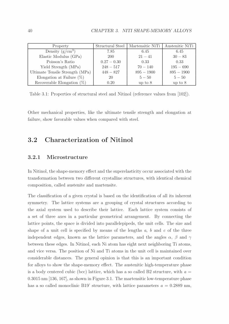
40 CHAPTER 3. NITI SHAPE-MEMORY ALLOYS
Property Structural Steel Martensitic NiTi Austenitic NiTi
Density (g/cm3) 7.85 6.45 6.45Elastic Modulus (GPa) 200 21 − 41 30− 83
Poisson’s Ratio 0.27 − 0.30 0.33 0.33Yield Strength (MPa) 248 − 517 70− 140 195 − 690
Ultimate Tensile Strength (MPa) 448 − 827 895 − 1900 895 − 1900Elongation at Failure (%) 20 5− 50 5− 50Recoverable Elongation (%) 0.20 up to 8 up to 8
Table 3.1: Properties of structural steel and Nitinol (reference values from [102]).
Other mechanical properties, like the ultimate tensile strength and elongation at
failure, show favorable values when compared with steel.
3.2 Characterization of Nitinol
3.2.1 Microstructure
In Nitinol, the shape-memory effect and the superelasticity occur associated with the
transformation between two different crystalline structures, with identical chemical
composition, called austenite and martensite.
The classification of a given crystal is based on the identification of all its inherent
symmetry. The lattice systems are a grouping of crystal structures according to
the axial system used to describe their lattice. Each lattice system consists of
a set of three axes in a particular geometrical arrangement. By connecting the
lattice points, the space is divided into parallelepipeds, the unit cells. The size and
shape of a unit cell is specified by means of the lengths a, b and c of the three
independent edges, known as the lattice parameters, and the angles α, β and γ
between these edges. In Nitinol, each Ni atom has eight next neighboring Ti atoms,
and vice versa. The position of Ni and Ti atoms in the unit cell is maintained over
considerable distances. The general opinion is that this is an important condition
for alloys to show the shape-memory effect. The austenitic high-temperature phase
is a body centered cubic (bcc) lattice, which has a so called B2 structure, with a =
0.3015 nm [136, 167], as shown in Figure 3.1. The martensitic low-temperature phase
has a so called monoclinic B19’ structure, with lattice parameters a = 0.2889 nm,
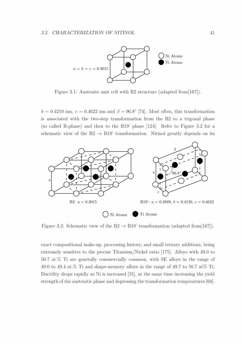
3.2. CHARACTERIZATION OF NITINOL 41
Ti Atoms
Ni Atoms
a = b = c = 0.3015
Figure 3.1: Austenite unit cell with B2 structure (adapted from[167]).
b = 0.4210 nm, c = 0.4622 nm and β = 96.8 [74]. Most often, this transformation
is associated with the two-step transformation from the B2 to a trigonal phase
(so called R-phase) and then to the B19’ phase [124]. Refer to Figure 3.2 for a
schematic view of the B2 → B19’ transformation. Nitinol greatly depends on its
Ni Atoms Ti Atoms
B2: a = 0.3015 B19’: a = 0.2889, b = 0.4120, c = 0.4622
a
b
c
96.8
a
Figure 3.2: Schematic view of the B2 → B19’ transformation (adapted from[167]).
exact compositional make-up, processing history, and small ternary additions, being
extremely sensitive to the precise Titanium/Nickel ratio [175]. Alloys with 49.0 to
50.7 at.% Ti are generally commercially common, with SE alloys in the range of
49.0 to 49.4 at.% Ti and shape-memory alloys in the range of 49.7 to 50.7 at% Ti.
Ductility drops rapidly as Ni is increased [55], at the same time increasing the yield
strength of the austenitic phase and depressing the transformation temperatures [60].
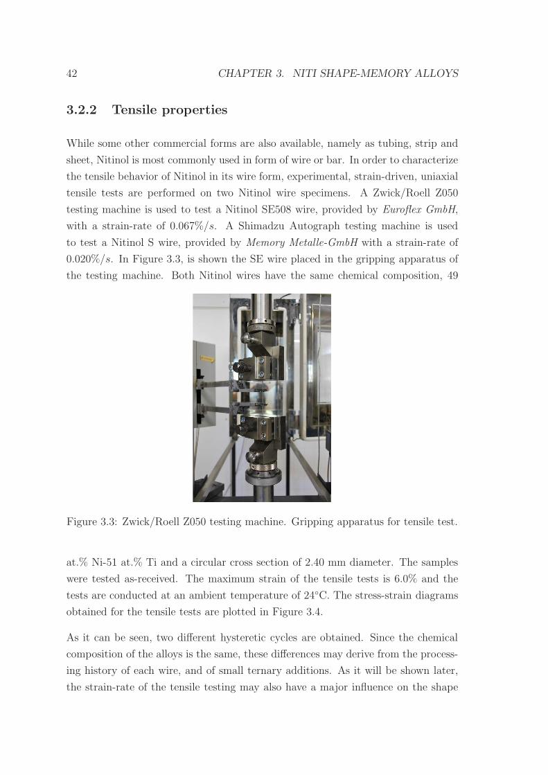
42 CHAPTER 3. NITI SHAPE-MEMORY ALLOYS
3.2.2 Tensile properties
While some other commercial forms are also available, namely as tubing, strip and
sheet, Nitinol is most commonly used in form of wire or bar. In order to characterize
the tensile behavior of Nitinol in its wire form, experimental, strain-driven, uniaxial
tensile tests are performed on two Nitinol wire specimens. A Zwick/Roell Z050
testing machine is used to test a Nitinol SE508 wire, provided by Euroflex GmbH,
with a strain-rate of 0.067%/s. A Shimadzu Autograph testing machine is used
to test a Nitinol S wire, provided by Memory Metalle-GmbH with a strain-rate of
0.020%/s. In Figure 3.3, is shown the SE wire placed in the gripping apparatus of
the testing machine. Both Nitinol wires have the same chemical composition, 49
Figure 3.3: Zwick/Roell Z050 testing machine. Gripping apparatus for tensile test.
at.% Ni-51 at.% Ti and a circular cross section of 2.40 mm diameter. The samples
were tested as-received. The maximum strain of the tensile tests is 6.0% and the
tests are conducted at an ambient temperature of 24C. The stress-strain diagrams
obtained for the tensile tests are plotted in Figure 3.4.
As it can be seen, two different hysteretic cycles are obtained. Since the chemical
composition of the alloys is the same, these differences may derive from the process-
ing history of each wire, and of small ternary additions. As it will be shown later,
the strain-rate of the tensile testing may also have a major influence on the shape
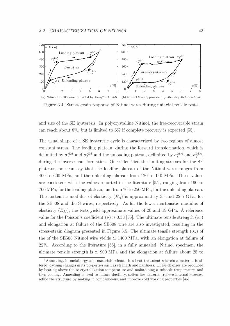
3.2. CHARACTERIZATION OF NITINOL 43
1 2 4 5 6 7 83
720
240
360
480
600
120
0
σ[MPa]
ε[%]σMAs
Euroflex
Unloading plateau
σAMs
σMAs
Loading plateau σAMf
0
(a) Nitinol SE 508 wire, provided by Euroflex GmbH
1 2 4 5 6 7 83
720
240
360
480
600
120
0
σ[MPa]
ε[%]Unloading plateau
MemoryMetalle
0
σMAs
σAMs
σAMfLoading plateau
σMAs
(b) Nitinol S wire, provided by Memory Metalle-GmbH
Figure 3.4: Stress-strain response of Nitinol wires during uniaxial tensile tests.
and size of the SE hysteresis. In polycrystalline Nitinol, the free-recoverable strain
can reach about 8%, but is limited to 6% if complete recovery is expected [55].
The usual shape of a SE hysteretic cycle is characterized by two regions of almost
constant stress. The loading plateau, during the forward transformation, which is
delimited by σAMs and σAM
f and the unloading plateau, delimited by σMAs and σMA
f ,
during the inverse transformation. Once identified the limiting stresses for the SE
plateaus, one can say that the loading plateau of the Nitinol wires ranges from
400 to 600 MPa, and the unloading plateau from 120 to 140 MPa. These values
are consistent with the values reported in the literature [55], ranging from 190 to
700 MPa, for the loading plateau, and from 70 to 250 MPa, for the unloading plateau.
The austenitic modulus of elasticity (EA) is approximately 35 and 22.5 GPa, for
the SE508 and the S wires, respectively. As for the lower martensitic modulus of
elasticity (EM), the tests yield approximate values of 20 and 19 GPa. A reference
value for the Poisson’s coefficient (ν) is 0.33 [55]. The ultimate tensile strength (σu)
and elongation at failure of the SE508 wire are also investigated, resulting in the
stress-strain diagram presented in Figure 3.5. The ultimate tensile strength (σu) of
the of the SE508 Nitinol wire yields ≃ 1400 MPa, with an elongation at failure of
22%. According to the literature [55], in a fully annealed1 Nitinol specimen, the
ultimate tensile strength is ≃ 900 MPa and the elongation at failure about 25 to
1Annealing, in metallurgy and materials science, is a heat treatment wherein a material is al-tered, causing changes in its properties such as strength and hardness. These changes are producedby heating above the re-crystallization temperature and maintaining a suitable temperature, andthen cooling. Annealing is used to induce ductility, soften the material, relieve internal stresses,refine the structure by making it homogeneous, and improve cold working properties [45].
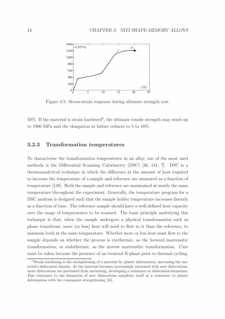
44 CHAPTER 3. NITI SHAPE-MEMORY ALLOYS
σ[MPa]
ε[%]
σu
0 5 10 15 20 25
1680
1440
1200
960
720
480
240
0
Figure 3.5: Stress-strain response during ultimate strength test.
50%. If the material is strain hardened2, the ultimate tensile strength may reach up
to 1900 MPa and the elongation at failure reduces to 5 to 10%.
3.2.3 Transformation temperatures
To characterize the transformation temperatures in an alloy, one of the most used
methods is the Differential Scanning Calorimetry (DSC) [36, 141, ?]. DSC is a
thermoanalytical technique in which the difference in the amount of heat required
to increase the temperature of a sample and reference are measured as a function of
temperature [138]. Both the sample and reference are maintained at nearly the same
temperature throughout the experiment. Generally, the temperature program for a
DSC analysis is designed such that the sample holder temperature increases linearly
as a function of time. The reference sample should have a well-defined heat capacity
over the range of temperatures to be scanned. The basic principle underlying this
technique is that, when the sample undergoes a physical transformation such as
phase transitions, more (or less) heat will need to flow to it than the reference, to
maintain both at the same temperature. Whether more or less heat must flow to the
sample depends on whether the process is exothermic, as the forward martensitic
transformation, or endothermic, as the inverse martensitic transformation. Care
must be taken because the presence of an eventual R-phase prior to thermal cycling,
2Strain hardening is the strengthening of a material by plastic deformation, increasing the ma-terial’s dislocation density. As the material becomes increasingly saturated with new dislocations,more dislocations are prevented from nucleating, developing a resistance to dislocation-formation.This resistance to the formation of new dislocations manifests itself as a resistance to plasticdeformation with the consequent strengthening [45].
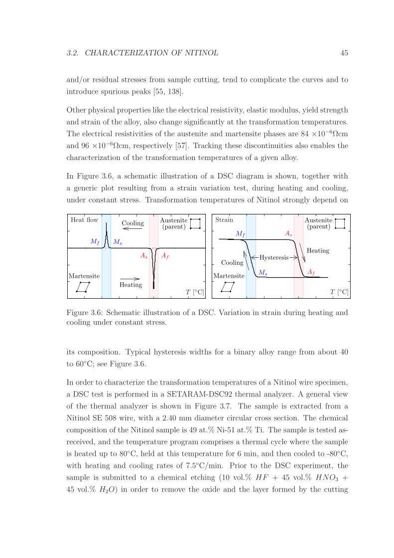
3.2. CHARACTERIZATION OF NITINOL 45
and/or residual stresses from sample cutting, tend to complicate the curves and to
introduce spurious peaks [55, 138].
Other physical properties like the electrical resistivity, elastic modulus, yield strength
and strain of the alloy, also change significantly at the transformation temperatures.
The electrical resistivities of the austenite and martensite phases are 84 ×10−6Ωcm
and 96 ×10−6Ωcm, respectively [57]. Tracking these discontinuities also enables the
characterization of the transformation temperatures of a given alloy.
In Figure 3.6, a schematic illustration of a DSC diagram is shown, together with
a generic plot resulting from a strain variation test, during heating and cooling,
under constant stress. Transformation temperatures of Nitinol strongly depend on
Austenite(parent)
Cooling
Heating
Austenite(parent)
Hysteresis
Mf Ms
As Af
T [C]
Martensite Martensite
Heating
Cooling
T [C]
Mf
Ms
As
Af
Heat flow Strain
Figure 3.6: Schematic illustration of a DSC. Variation in strain during heating andcooling under constant stress.
its composition. Typical hysteresis widths for a binary alloy range from about 40
to 60C; see Figure 3.6.
In order to characterize the transformation temperatures of a Nitinol wire specimen,
a DSC test is performed in a SETARAM-DSC92 thermal analyzer. A general view
of the thermal analyzer is shown in Figure 3.7. The sample is extracted from a
Nitinol SE 508 wire, with a 2.40 mm diameter circular cross section. The chemical
composition of the Nitinol sample is 49 at.% Ni-51 at.% Ti. The sample is tested as-
received, and the temperature program comprises a thermal cycle where the sample
is heated up to 80C, held at this temperature for 6 min, and then cooled to -80C,
with heating and cooling rates of 7.5C/min. Prior to the DSC experiment, the
sample is submitted to a chemical etching (10 vol.% HF + 45 vol.% HNO3 +
45 vol.% H2O) in order to remove the oxide and the layer formed by the cutting
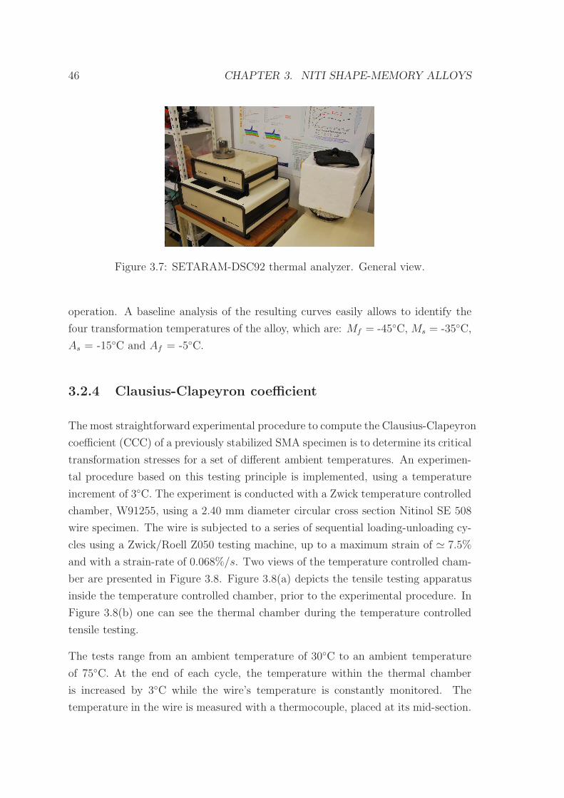
46 CHAPTER 3. NITI SHAPE-MEMORY ALLOYS
Figure 3.7: SETARAM-DSC92 thermal analyzer. General view.
operation. A baseline analysis of the resulting curves easily allows to identify the
four transformation temperatures of the alloy, which are: Mf = -45C, Ms = -35C,
As = -15C and Af = -5C.
3.2.4 Clausius-Clapeyron coefficient
The most straightforward experimental procedure to compute the Clausius-Clapeyron
coefficient (CCC) of a previously stabilized SMA specimen is to determine its critical
transformation stresses for a set of different ambient temperatures. An experimen-
tal procedure based on this testing principle is implemented, using a temperature
increment of 3C. The experiment is conducted with a Zwick temperature controlled
chamber, W91255, using a 2.40 mm diameter circular cross section Nitinol SE 508
wire specimen. The wire is subjected to a series of sequential loading-unloading cy-
cles using a Zwick/Roell Z050 testing machine, up to a maximum strain of ≃ 7.5%
and with a strain-rate of 0.068%/s. Two views of the temperature controlled cham-
ber are presented in Figure 3.8. Figure 3.8(a) depicts the tensile testing apparatus
inside the temperature controlled chamber, prior to the experimental procedure. In
Figure 3.8(b) one can see the thermal chamber during the temperature controlled
tensile testing.
The tests range from an ambient temperature of 30C to an ambient temperature
of 75C. At the end of each cycle, the temperature within the thermal chamber
is increased by 3C while the wire’s temperature is constantly monitored. The
temperature in the wire is measured with a thermocouple, placed at its mid-section.
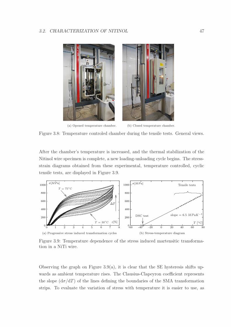
3.2. CHARACTERIZATION OF NITINOL 47
(a) Opened temperature chamber. (b) Closed temperature chamber.
Figure 3.8: Temperature controled chamber during the tensile tests. General views.
After the chamber’s temperature is increased, and the thermal stabilization of the
Nitinol wire specimen is complete, a new loading-unloading cycle begins. The stress-
strain diagrams obtained from these experimental, temperature controlled, cyclic
tensile tests, are displayed in Figure 3.9.
0
800
600
400
200
σ[MPa]
T = 75C
∆T
T = 30C ε[%]
0 6
1000
1 2 3 4 5 7 8
(a) Progressive stress induced transformation cycles
T [C]
σ[MPa]
-60 80
1000
800
600
400
200
0-40 -20 0 20 40 60
Tensile tests
slope = 6.5 MPaK−1DSC test
(b) Stress-temperature diagram
Figure 3.9: Temperature dependence of the stress induced martensitic transforma-tion in a NiTi wire.
Observing the graph on Figure 3.9(a), it is clear that the SE hysteresis shifts up-
wards as ambient temperature rises. The Clausius-Clapeyron coefficient represents
the slope (dσ/dT ) of the lines defining the boundaries of the SMA transformation
strips. To evaluate the variation of stress with temperature it is easier to use, as
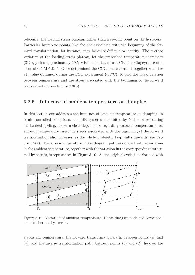
48 CHAPTER 3. NITI SHAPE-MEMORY ALLOYS
reference, the loading stress plateau, rather than a specific point on the hysteresis.
Particular hysteretic points, like the one associated with the beginning of the for-
ward transformation, for instance, may be quite difficult to identify. The average
variation of the loading stress plateau, for the prescribed temperature increment
(3C), yields approximately 19.5 MPa. This leads to a Clausius-Clapeyron coeffi-
cient of 6.5 MPaK−1. Once determined the CCC, one can use it together with the
Ms value obtained during the DSC experiment (-35C), to plot the linear relation
between temperature and the stress associated with the beginning of the forward
transformation; see Figure 3.9(b).
3.2.5 Influence of ambient temperature on damping
In this section one addresses the influence of ambient temperature on damping, in
strain-controlled conditions. The SE hysteresis exhibited by Nitinol wires during
mechanical cycling, shows a clear dependence regarding ambient temperature. As
ambient temperature rises, the stress associated with the beginning of the forward
transformation also increases, as the whole hysteretic loop shifts upwards; see Fig-
ure 3.9(a). The stress-temperature phase diagram path associated with a variation
in the ambient temperature, together with the variation in the corresponding isother-
mal hysteresis, is represented in Figure 3.10. As the original cycle is performed with
o
ε
σ
a
a’
AsM t,dA
εmax
Af
[M ]
Md
AT0 T1
Mf
[A]
b’
a’
b’
a
b Msb
c
d
d’
c’ c’
d’c
dT
σ
Figure 3.10: Variation of ambient temperature. Phase diagram path and correspon-dent isothermal hysteresis.
a constant temperature, the forward transformation path, between points (a) and
(b), and the inverse transformation path, between points (c) and (d), lie over the
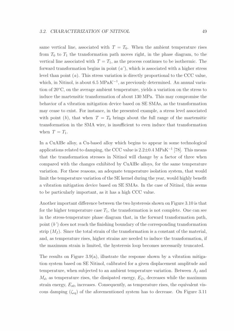
3.2. CHARACTERIZATION OF NITINOL 49
same vertical line, associated with T = T0. When the ambient temperature rises
from T0 to T1 the transformation path moves right, in the phase diagram, to the
vertical line associated with T = T1, as the process continues to be isothermic. The
forward transformation begins in point (a’ ), which is associated with a higher stress
level than point (a). This stress variation is directly proportional to the CCC value,
which, in Nitinol, is about 6.5 MPaK−1, as previously determined. An annual varia-
tion of 20C, on the average ambient temperature, yields a variation on the stress to
induce the martensitic transformation of about 130 MPa. This may compromise the
behavior of a vibration mitigation device based on SE SMAs, as the transformation
may cease to exist. For instance, in the presented example, a stress level associated
with point (b), that when T = T0 brings about the full range of the martensitic
transformation in the SMA wire, is insufficient to even induce that transformation
when T = T1.
In a CuAlBe alloy, a Cu-based alloy which begins to appear in some technological
applications related to damping, the CCC value is 2.2±0.4 MPaK−1 [78]. This means
that the transformation stresses in Nitinol will change by a factor of three when
compared with the changes exhibited by CuAlBe alloys, for the same temperature
variation. For these reasons, an adequate temperature isolation system, that would
limit the temperature variation of the SE kernel during the year, would highly benefit
a vibration mitigation device based on SE SMAs. In the case of Nitinol, this seems
to be particularly important, as it has a high CCC value.
Another important difference between the two hysteresis shown on Figure 3.10 is that
for the higher temperature case T1, the transformation is not complete. One can see
in the stress-temperature phase diagram that, in the forward transformation path,
point (b’ ) does not reach the finishing boundary of the corresponding transformation
strip (Mf ). Since the total strain of the transformation is a constant of the material,
and, as temperature rises, higher strains are needed to induce the transformation, if
the maximum strain is limited, the hysteresis loop becomes necessarily truncated.
The results on Figure 3.9(a), illustrate the response shown by a vibration mitiga-
tion system based on SE Nitinol, calibrated for a given displacement amplitude and
temperature, when subjected to an ambient temperature variation. Between Af and
Md, as temperature rises, the dissipated energy, ED, decreases while the maximum
strain energy, Es0, increases. Consequently, as temperature rises, the equivalent vis-
cous damping (ζeq) of the aforementioned system has to decrease. On Figure 3.11
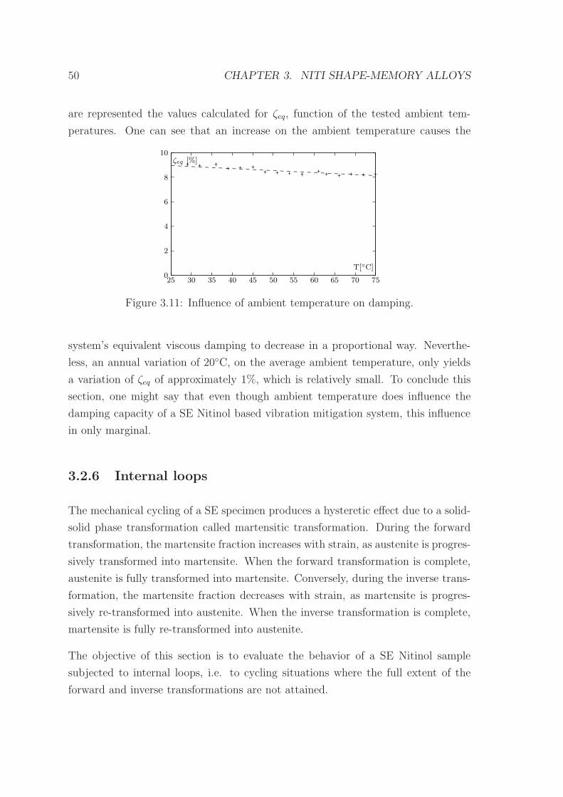
50 CHAPTER 3. NITI SHAPE-MEMORY ALLOYS
are represented the values calculated for ζeq, function of the tested ambient tem-
peratures. One can see that an increase on the ambient temperature causes the
10
8
6
4
2
025 30 35 40 45 50 55 60 65 70 75
T[C]
ζeq [%]
Figure 3.11: Influence of ambient temperature on damping.
system’s equivalent viscous damping to decrease in a proportional way. Neverthe-
less, an annual variation of 20C, on the average ambient temperature, only yields
a variation of ζeq of approximately 1%, which is relatively small. To conclude this
section, one might say that even though ambient temperature does influence the
damping capacity of a SE Nitinol based vibration mitigation system, this influence
in only marginal.
3.2.6 Internal loops
The mechanical cycling of a SE specimen produces a hysteretic effect due to a solid-
solid phase transformation called martensitic transformation. During the forward
transformation, the martensite fraction increases with strain, as austenite is progres-
sively transformed into martensite. When the forward transformation is complete,
austenite is fully transformed into martensite. Conversely, during the inverse trans-
formation, the martensite fraction decreases with strain, as martensite is progres-
sively re-transformed into austenite. When the inverse transformation is complete,
martensite is fully re-transformed into austenite.
The objective of this section is to evaluate the behavior of a SE Nitinol sample
subjected to internal loops, i.e. to cycling situations where the full extent of the
forward and inverse transformations are not attained.
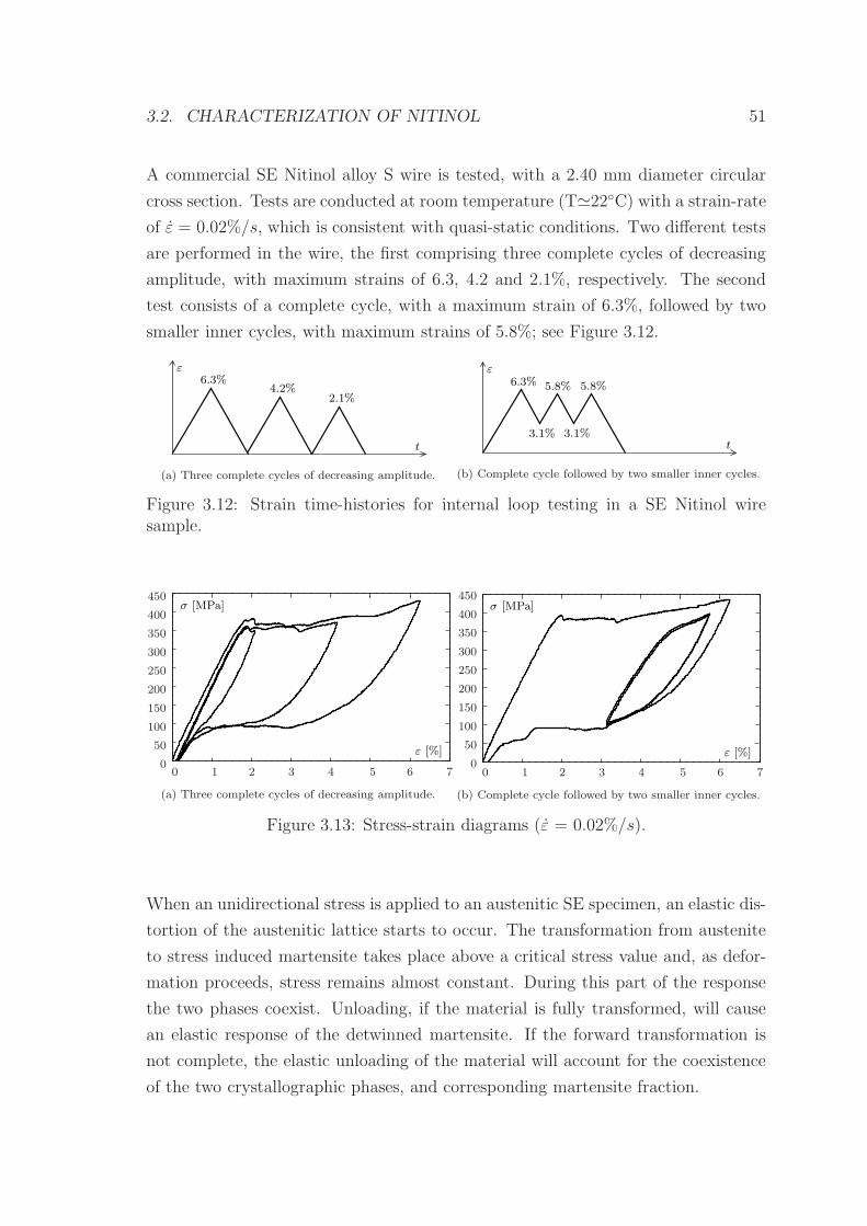
3.2. CHARACTERIZATION OF NITINOL 51
A commercial SE Nitinol alloy S wire is tested, with a 2.40 mm diameter circular
cross section. Tests are conducted at room temperature (T≃22C) with a strain-rate
of ε = 0.02%/s, which is consistent with quasi-static conditions. Two different tests
are performed in the wire, the first comprising three complete cycles of decreasing
amplitude, with maximum strains of 6.3, 4.2 and 2.1%, respectively. The second
test consists of a complete cycle, with a maximum strain of 6.3%, followed by two
smaller inner cycles, with maximum strains of 5.8%; see Figure 3.12.
6.3%4.2%
2.1%
t
ε
(a) Three complete cycles of decreasing amplitude.
ε6.3% 5.8% 5.8%
t3.1%3.1%
(b) Complete cycle followed by two smaller inner cycles.
Figure 3.12: Strain time-histories for internal loop testing in a SE Nitinol wiresample.
σ [MPa]
ε [%]
70 1 2 3 4 5 60
50
100
150
200
250
300
350
400
450
(a) Three complete cycles of decreasing amplitude.
σ [MPa]
ε [%]0
50
100
150
200
250
300
350
400
450
70 1 2 3 4 5 6
(b) Complete cycle followed by two smaller inner cycles.
Figure 3.13: Stress-strain diagrams (ε = 0.02%/s).
When an unidirectional stress is applied to an austenitic SE specimen, an elastic dis-
tortion of the austenitic lattice starts to occur. The transformation from austenite
to stress induced martensite takes place above a critical stress value and, as defor-
mation proceeds, stress remains almost constant. During this part of the response
the two phases coexist. Unloading, if the material is fully transformed, will cause
an elastic response of the detwinned martensite. If the forward transformation is
not complete, the elastic unloading of the material will account for the coexistence
of the two crystallographic phases, and corresponding martensite fraction.
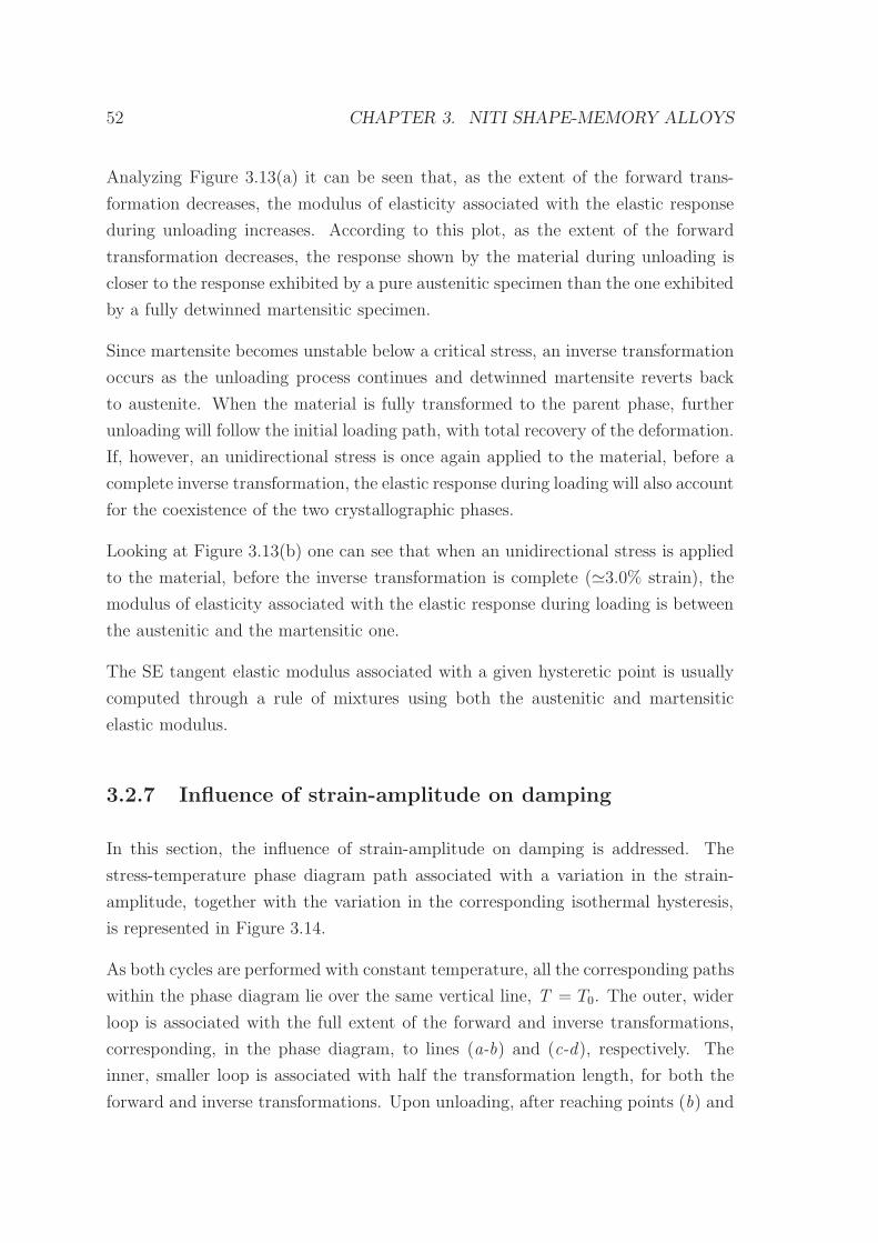
52 CHAPTER 3. NITI SHAPE-MEMORY ALLOYS
Analyzing Figure 3.13(a) it can be seen that, as the extent of the forward trans-
formation decreases, the modulus of elasticity associated with the elastic response
during unloading increases. According to this plot, as the extent of the forward
transformation decreases, the response shown by the material during unloading is
closer to the response exhibited by a pure austenitic specimen than the one exhibited
by a fully detwinned martensitic specimen.
Since martensite becomes unstable below a critical stress, an inverse transformation
occurs as the unloading process continues and detwinned martensite reverts back
to austenite. When the material is fully transformed to the parent phase, further
unloading will follow the initial loading path, with total recovery of the deformation.
If, however, an unidirectional stress is once again applied to the material, before a
complete inverse transformation, the elastic response during loading will also account
for the coexistence of the two crystallographic phases.
Looking at Figure 3.13(b) one can see that when an unidirectional stress is applied
to the material, before the inverse transformation is complete (≃3.0% strain), the
modulus of elasticity associated with the elastic response during loading is between
the austenitic and the martensitic one.
The SE tangent elastic modulus associated with a given hysteretic point is usually
computed through a rule of mixtures using both the austenitic and martensitic
elastic modulus.
3.2.7 Influence of strain-amplitude on damping
In this section, the influence of strain-amplitude on damping is addressed. The
stress-temperature phase diagram path associated with a variation in the strain-
amplitude, together with the variation in the corresponding isothermal hysteresis,
is represented in Figure 3.14.
As both cycles are performed with constant temperature, all the corresponding paths
within the phase diagram lie over the same vertical line, T = T0. The outer, wider
loop is associated with the full extent of the forward and inverse transformations,
corresponding, in the phase diagram, to lines (a-b) and (c-d), respectively. The
inner, smaller loop is associated with half the transformation length, for both the
forward and inverse transformations. Upon unloading, after reaching points (b) and
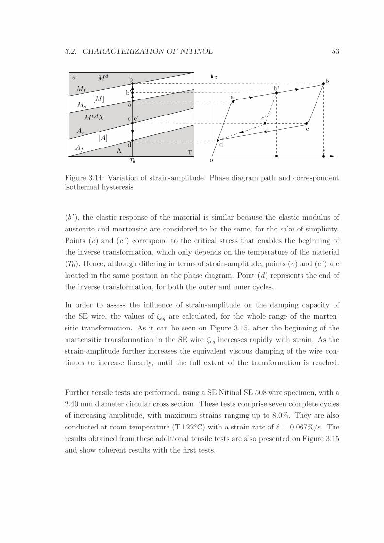
3.2. CHARACTERIZATION OF NITINOL 53
o
b
c
d
aa
ε
σ
T
σ
T0
Md
A
c
d[A]
[M ]
M t,dA
Ms
Mf
As
Af
b’
c’c’
b’
b
Figure 3.14: Variation of strain-amplitude. Phase diagram path and correspondentisothermal hysteresis.
(b’ ), the elastic response of the material is similar because the elastic modulus of
austenite and martensite are considered to be the same, for the sake of simplicity.
Points (c) and (c’ ) correspond to the critical stress that enables the beginning of
the inverse transformation, which only depends on the temperature of the material
(T0). Hence, although differing in terms of strain-amplitude, points (c) and (c’ ) are
located in the same position on the phase diagram. Point (d) represents the end of
the inverse transformation, for both the outer and inner cycles.
In order to assess the influence of strain-amplitude on the damping capacity of
the SE wire, the values of ζeq are calculated, for the whole range of the marten-
sitic transformation. As it can be seen on Figure 3.15, after the beginning of the
martensitic transformation in the SE wire ζeq increases rapidly with strain. As the
strain-amplitude further increases the equivalent viscous damping of the wire con-
tinues to increase linearly, until the full extent of the transformation is reached.
Further tensile tests are performed, using a SE Nitinol SE 508 wire specimen, with a
2.40 mm diameter circular cross section. These tests comprise seven complete cycles
of increasing amplitude, with maximum strains ranging up to 8.0%. They are also
conducted at room temperature (T±22C) with a strain-rate of ε = 0.067%/s. The
results obtained from these additional tensile tests are also presented on Figure 3.15
and show coherent results with the first tests.
54 CHAPTER 3. NITI SHAPE-MEMORY ALLOYS
Euroflex
MemoryMetalle
0
20
16
12
8
4
ε[%]
ζeq [%]
61 2 3 4 5 7 80
Figure 3.15: Influence of strain-amplitude on damping.
3.2.8 Self-heating on mechanical cycling
When a fluid/solid body is at a different temperature than its surroundings, transfer
of thermal energy, also known as heat transfer, or heat exchange, occurs in such a
way that the body and the surroundings reach a thermal equilibrium. Heat transfer
always occurs from a higher-temperature object to a cooler temperature one. Energy
transfer by heat can occur between objects by radiation, conduction and convection.
Convection is usually the dominant form of heat transfer in liquids and gases. This
is a term used to characterize the combined effects of conduction and fluid flow.
Two types of convection are commonly distinguished: free convection, in which
gravity and buoyancy forces drive the fluid movement, and forced convection, where
a fan, stirrer, or other means are used to move the fluid. In natural convection,
fluid surrounding a heat source receives heat, becomes less dense and rises. The
surrounding, cooler fluid then moves to replace it. This cooler fluid is then heated
and the process continues, forming a convection current. The driving force for
natural convection is buoyancy, a result of differences in fluid density [76].
During the cyclic deformation of a SMA specimen, self-heating depends on the
balance between the total generated energy (enthalpy of transformation and internal
friction) and the dissipated energy by heat transfer.
To illustrate how the strain-rate of the dynamic loading may influence the temper-
ature variation of a SE specimen during a cyclic test, as well as the shape of its
corresponding hysteretic loop, a series of experimental tensile tests are conducted.
These experimental tests comprise four different strain-rates, 0.008, 0.067, 0.250
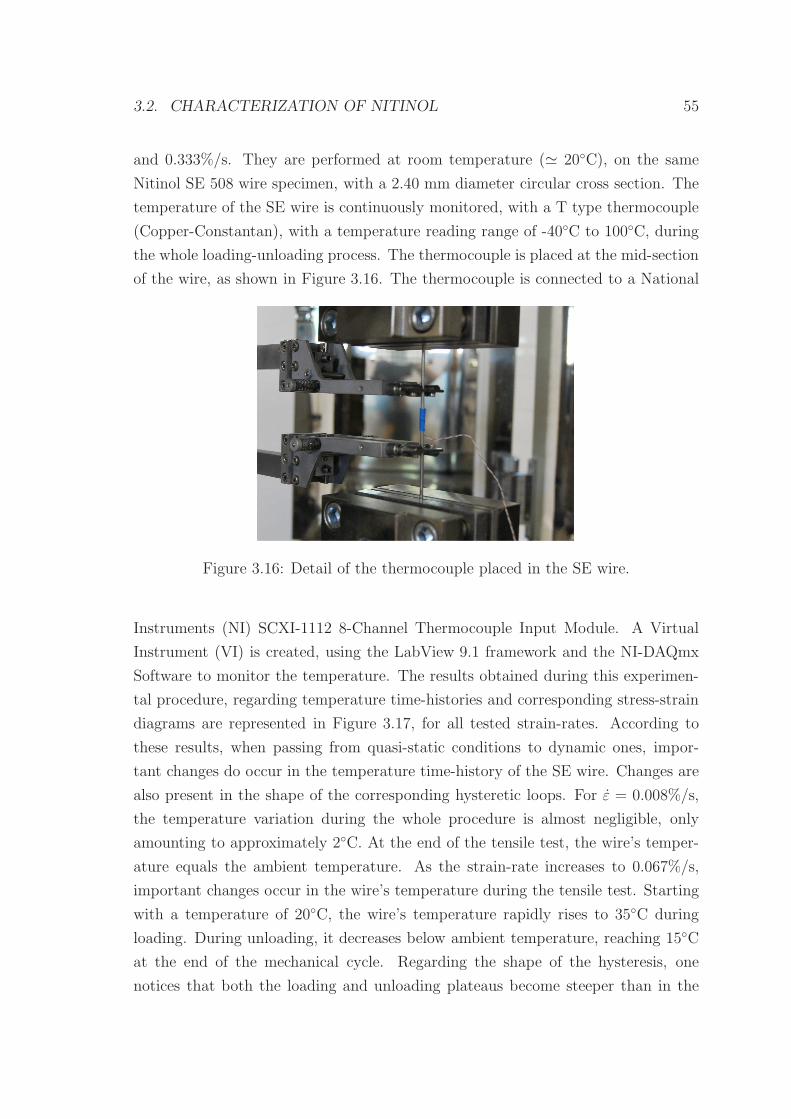
3.2. CHARACTERIZATION OF NITINOL 55
and 0.333%/s. They are performed at room temperature (≃ 20C), on the same
Nitinol SE 508 wire specimen, with a 2.40 mm diameter circular cross section. The
temperature of the SE wire is continuously monitored, with a T type thermocouple
(Copper-Constantan), with a temperature reading range of -40C to 100C, during
the whole loading-unloading process. The thermocouple is placed at the mid-section
of the wire, as shown in Figure 3.16. The thermocouple is connected to a National
Figure 3.16: Detail of the thermocouple placed in the SE wire.
Instruments (NI) SCXI-1112 8-Channel Thermocouple Input Module. A Virtual
Instrument (VI) is created, using the LabView 9.1 framework and the NI-DAQmx
Software to monitor the temperature. The results obtained during this experimen-
tal procedure, regarding temperature time-histories and corresponding stress-strain
diagrams are represented in Figure 3.17, for all tested strain-rates. According to
these results, when passing from quasi-static conditions to dynamic ones, impor-
tant changes do occur in the temperature time-history of the SE wire. Changes are
also present in the shape of the corresponding hysteretic loops. For ε = 0.008%/s,
the temperature variation during the whole procedure is almost negligible, only
amounting to approximately 2C. At the end of the tensile test, the wire’s temper-
ature equals the ambient temperature. As the strain-rate increases to 0.067%/s,
important changes occur in the wire’s temperature during the tensile test. Starting
with a temperature of 20C, the wire’s temperature rapidly rises to 35C during
loading. During unloading, it decreases below ambient temperature, reaching 15C
at the end of the mechanical cycle. Regarding the shape of the hysteresis, one
notices that both the loading and unloading plateaus become steeper than in the
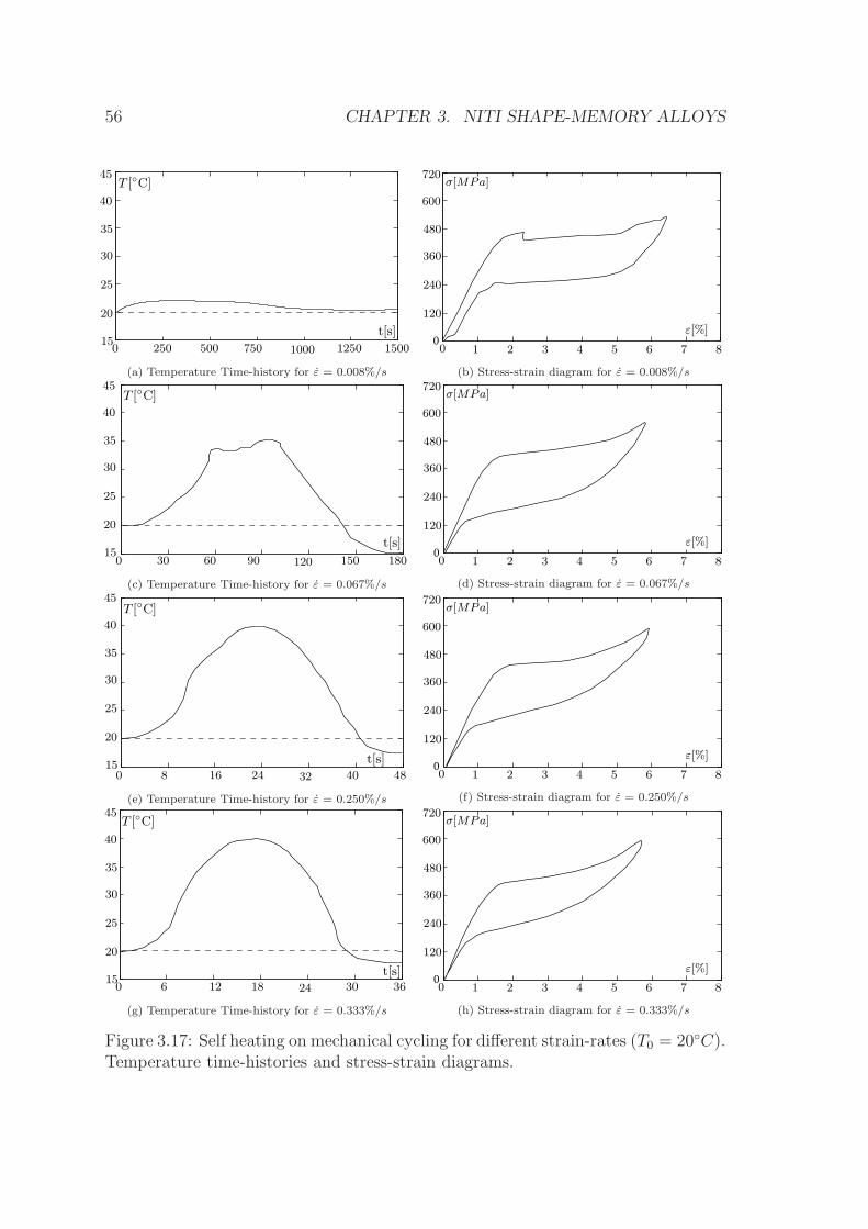
56 CHAPTER 3. NITI SHAPE-MEMORY ALLOYS
0 250 500 750 1000 1250 1500
20
45
25
30
35
40
15
T [C]
t[s]
(a) Temperature Time-history for ε = 0.008%/s
0
720
240
360
480
600
120
1 2 4 5 6 7 83
ε[%]
σ[MPa]
0
(b) Stress-strain diagram for ε = 0.008%/s
0 30 60 90 120 150 180
20
45
15
40
35
30
25
T [C]
t[s]
(c) Temperature Time-history for ε = 0.067%/s
01 2 4 5 6 7 83
ε[%]
σ[MPa]720
240
360
480
600
120
0
(d) Stress-strain diagram for ε = 0.067%/s
32 40 480 16 248
20
45
15
40
35
30
25
T [C]
t[s]
(e) Temperature Time-history for ε = 0.250%/s
01 2 4 5 6 7 83
ε[%]
σ[MPa]720
240
360
480
600
120
0
(f) Stress-strain diagram for ε = 0.250%/s
20
45
150 36302418126
40
35
30
25
T [C]
t[s]
(g) Temperature Time-history for ε = 0.333%/s
01 2 4 5 6 7 83
ε[%]
σ[MPa]720
240
360
480
600
120
0
(h) Stress-strain diagram for ε = 0.333%/s
Figure 3.17: Self heating on mechanical cycling for different strain-rates (T0 = 20C).Temperature time-histories and stress-strain diagrams.
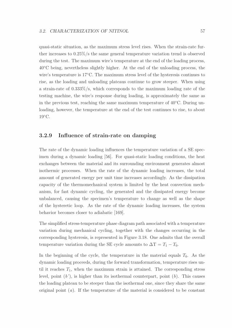
3.2. CHARACTERIZATION OF NITINOL 57
quasi-static situation, as the maximum stress level rises. When the strain-rate fur-
ther increases to 0.25%/s the same general temperature variation trend is observed
during the test. The maximum wire’s temperature at the end of the loading process,
40C being, nevertheless slightly higher. At the end of the unloading process, the
wire’s temperature is 17C. The maximum stress level of the hysteresis continues to
rise, as the loading and unloading plateaus continue to grow steeper. When using
a strain-rate of 0.333%/s, which corresponds to the maximum loading rate of the
testing machine, the wire’s response during loading, is approximately the same as
in the previous test, reaching the same maximum temperature of 40C. During un-
loading, however, the temperature at the end of the test continues to rise, to about
19C.
3.2.9 Influence of strain-rate on damping
The rate of the dynamic loading influences the temperature variation of a SE spec-
imen during a dynamic loading [56]. For quasi-static loading conditions, the heat
exchanges between the material and its surrounding environment generates almost
isothermic processes. When the rate of the dynamic loading increases, the total
amount of generated energy per unit time increases accordingly. As the dissipation
capacity of the thermomechanical system is limited by the heat convection mech-
anism, for fast dynamic cycling, the generated and the dissipated energy become
unbalanced, causing the specimen’s temperature to change as well as the shape
of the hysteretic loop. As the rate of the dynamic loading increases, the system
behavior becomes closer to adiabatic [169].
The simplified stress-temperature phase diagram path associated with a temperature
variation during mechanical cycling, together with the changes occurring in the
corresponding hysteresis, is represented in Figure 3.18. One admits that the overall
temperature variation during the SE cycle amounts to ∆T = T1 − T0.
In the beginning of the cycle, the temperature in the material equals T0. As the
dynamic loading proceeds, during the forward transformation, temperature rises un-
til it reaches T1, when the maximum strain is attained. The corresponding stress
level, point (b’ ), is higher than its isothermal counterpart, point (b). This causes
the loading plateau to be steeper than the isothermal one, since they share the same
original point (a). If the temperature of the material is considered to be constant
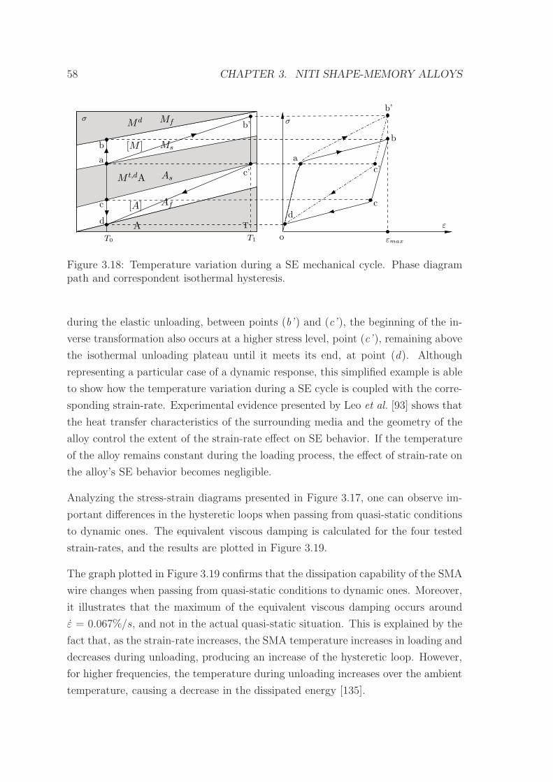
58 CHAPTER 3. NITI SHAPE-MEMORY ALLOYS
o
ε
σ
a
AsM t,dA
εmax
Af
[M ]
Md
AT0
Mf
[A]
b’
a
b Msb
c
d
c’
c
T
σ
d
T1
c’
b’
Figure 3.18: Temperature variation during a SE mechanical cycle. Phase diagrampath and correspondent isothermal hysteresis.
during the elastic unloading, between points (b’ ) and (c’ ), the beginning of the in-
verse transformation also occurs at a higher stress level, point (c’ ), remaining above
the isothermal unloading plateau until it meets its end, at point (d). Although
representing a particular case of a dynamic response, this simplified example is able
to show how the temperature variation during a SE cycle is coupled with the corre-
sponding strain-rate. Experimental evidence presented by Leo et al. [93] shows that
the heat transfer characteristics of the surrounding media and the geometry of the
alloy control the extent of the strain-rate effect on SE behavior. If the temperature
of the alloy remains constant during the loading process, the effect of strain-rate on
the alloy’s SE behavior becomes negligible.
Analyzing the stress-strain diagrams presented in Figure 3.17, one can observe im-
portant differences in the hysteretic loops when passing from quasi-static conditions
to dynamic ones. The equivalent viscous damping is calculated for the four tested
strain-rates, and the results are plotted in Figure 3.19.
The graph plotted in Figure 3.19 confirms that the dissipation capability of the SMA
wire changes when passing from quasi-static conditions to dynamic ones. Moreover,
it illustrates that the maximum of the equivalent viscous damping occurs around
ε = 0.067%/s, and not in the actual quasi-static situation. This is explained by the
fact that, as the strain-rate increases, the SMA temperature increases in loading and
decreases during unloading, producing an increase of the hysteretic loop. However,
for higher frequencies, the temperature during unloading increases over the ambient
temperature, causing a decrease in the dissipated energy [135].
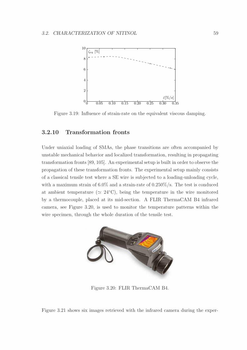
3.2. CHARACTERIZATION OF NITINOL 59
8
6
4
2
00.350.250.150.050 0.10 0.20 0.30
10ζeq [%]
ε[%/s]
Figure 3.19: Influence of strain-rate on the equivalent viscous damping.
3.2.10 Transformation fronts
Under uniaxial loading of SMAs, the phase transitions are often accompanied by
unstable mechanical behavior and localized transformation, resulting in propagating
transformation fronts [89, 105]. An experimental setup is built in order to observe the
propagation of these transformation fronts. The experimental setup mainly consists
of a classical tensile test where a SE wire is subjected to a loading-unloading cycle,
with a maximum strain of 6.0% and a strain-rate of 0.250%/s. The test is conduced
at ambient temperature (≃ 24C), being the temperature in the wire monitored
by a thermocouple, placed at its mid-section. A FLIR ThermaCAM B4 infrared
camera, see Figure 3.20, is used to monitor the temperature patterns within the
wire specimen, through the whole duration of the tensile test.
Figure 3.20: FLIR ThermaCAM B4.
Figure 3.21 shows six images retrieved with the infrared camera during the exper-
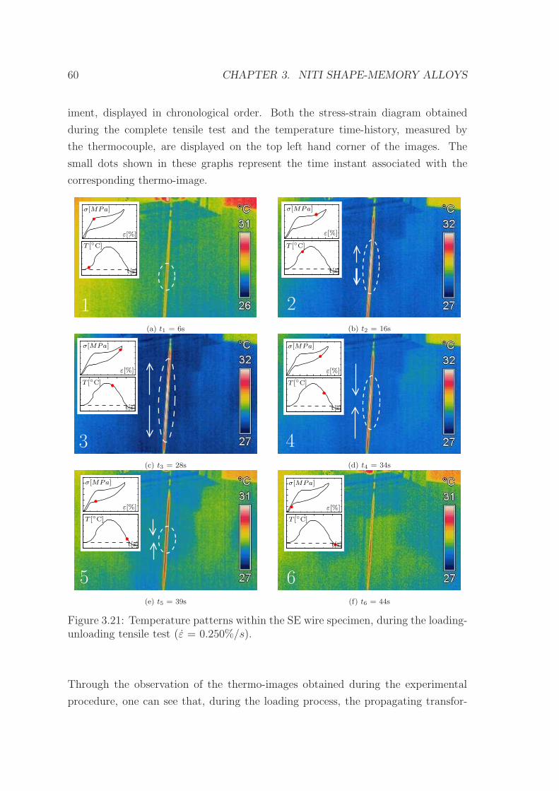
60 CHAPTER 3. NITI SHAPE-MEMORY ALLOYS
iment, displayed in chronological order. Both the stress-strain diagram obtained
during the complete tensile test and the temperature time-history, measured by
the thermocouple, are displayed on the top left hand corner of the images. The
small dots shown in these graphs represent the time instant associated with the
corresponding thermo-image.
1
σ[MPa]
ε[%]
t[s]
T [C]
(a) t1 = 6s
2
ε[%]
σ[MPa]
t[s]
T [C]
(b) t2 = 16s
3
σ[MPa]
ε[%]
t[s]
T [C]
(c) t3 = 28s
4
σ[MPa]
ε[%]
t[s]
T [C]
(d) t4 = 34s
5
σ[MPa]
ε[%]
t[s]
T [C]
(e) t5 = 39s
6
σ[MPa]
ε[%]
t[s]
T [C]
(f) t6 = 44s
Figure 3.21: Temperature patterns within the SE wire specimen, during the loading-unloading tensile test (ε = 0.250%/s).
Through the observation of the thermo-images obtained during the experimental
procedure, one can see that, during the loading process, the propagating transfor-
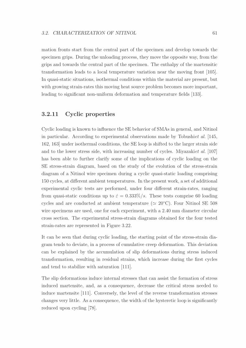
3.2. CHARACTERIZATION OF NITINOL 61
mation fronts start from the central part of the specimen and develop towards the
specimen grips. During the unloading process, they move the opposite way, from the
grips and towards the central part of the specimen. The enthalpy of the martensitic
transformation leads to a local temperature variation near the moving front [105].
In quasi-static situations, isothermal conditions within the material are present, but
with growing strain-rates this moving heat source problem becomes more important,
leading to significant non-uniform deformation and temperature fields [133].
3.2.11 Cyclic properties
Cyclic loading is known to influence the SE behavior of SMAs in general, and Nitinol
in particular. According to experimental observations made by Tobushiet al. [145,
162, 163] under isothermal conditions, the SE loop is shifted to the larger strain side
and to the lower stress side, with increasing number of cycles. Miyazakiet al. [107]
has been able to further clarify some of the implications of cyclic loading on the
SE stress-strain diagram, based on the study of the evolution of the stress-strain
diagram of a Nitinol wire specimen during a cyclic quasi-static loading comprising
150 cycles, at different ambient temperatures. In the present work, a set of additional
experimental cyclic tests are performed, under four different strain-rates, ranging
from quasi-static conditions up to ε = 0.333%/s. These tests comprise 60 loading
cycles and are conducted at ambient temperature (≃ 20C). Four Nitinol SE 508
wire specimens are used, one for each experiment, with a 2.40 mm diameter circular
cross section. The experimental stress-strain diagrams obtained for the four tested
strain-rates are represented in Figure 3.22.
It can be seen that during cyclic loading, the starting point of the stress-strain dia-
gram tends to deviate, in a process of cumulative creep deformation. This deviation
can be explained by the accumulation of slip deformations during stress induced
transformation, resulting in residual strains, which increase during the first cycles
and tend to stabilize with saturation [111].
The slip deformations induce internal stresses that can assist the formation of stress
induced martensite, and, as a consequence, decrease the critical stress needed to
induce martensite [111]. Conversely, the level of the reverse transformation stresses
changes very little. As a consequence, the width of the hysteretic loop is significantly
reduced upon cycling [78].
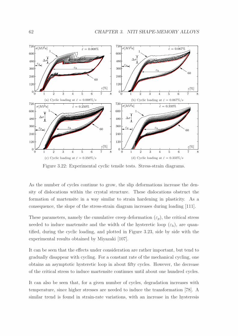
62 CHAPTER 3. NITI SHAPE-MEMORY ALLOYS
1
60
1 2 4 5 6 7 83
σ[MPa]
ε[%]
ε = 0.008%
εpεh
∆σ
720
240
360
480
600
120
00
(a) Cyclic loading at ε = 0.008%/s
1
60
1 2 4 5 6 7 830
ε[%]
σ[MPa]
∆σ
ε = 0.067%
εp
720
240
360
480
600
120
0
εh
(b) Cyclic loading at ε = 0.067%/s
60
1 2 4 5 6 7 830
σ[MPa]
ε[%]
1
720
240
360
480
600
120
0
εp εh
ε = 0.250%
∆σ
(c) Cyclic loading at ε = 0.250%/s
1 2 4 5 6 7 830
60
ε[%]
σ[MPa]
1
∆σ
εp
ε = 0.333%
εh
720
240
360
480
600
120
0
(d) Cyclic loading at ε = 0.333%/s
Figure 3.22: Experimental cyclic tensile tests. Stress-strain diagrams.
As the number of cycles continue to grow, the slip deformations increase the den-
sity of dislocations within the crystal structure. These dislocations obstruct the
formation of martensite in a way similar to strain hardening in plasticity. As a
consequence, the slope of the stress-strain diagram increases during loading [111].
These parameters, namely the cumulative creep deformation (εp), the critical stress
needed to induce martensite and the width of the hysteretic loop (εh), are quan-
tified, during the cyclic loading, and plotted in Figure 3.23, side by side with the
experimental results obtained by Miyazaki [107].
It can be seen that the effects under consideration are rather important, but tend to
gradually disappear with cycling. For a constant rate of the mechanical cycling, one
obtains an asymptotic hysteretic loop in about fifty cycles. However, the decrease
of the critical stress to induce martensite continues until about one hundred cycles.
It can also be seen that, for a given number of cycles, degradation increases with
temperature, since higher stresses are needed to induce the transformation [78]. A
similar trend is found in strain-rate variations, with an increase in the hysteresis

3.2. CHARACTERIZATION OF NITINOL 63
10 20 30 40 50 600
σ
εp
ε
0.008%/s0.067%/s0.250%/s0.333%/s
0
0.2
0.4
0.6
0.8
1.2Cycles
εp[%]
1.0
(a) Cumulative creep. Strain-rate variation
12C
36C26C
σ
εp
ε
εp[%]
Cycles
0 50 100 150
0.0
1.0
1.5
0.5
(b) Cumulative creep. Temperature variation [107]
10 20 30 40 50 600
N cycleσσ
1 cycle
∆σ = σ1 − σN
σ1
ε ε
0.008%/s0.067%/s0.250%/s0.333%/s
0
20
40
60
80
100
120
160
140
∆σ [MPa]
Cycles
(c) Critical stress to form SIM. Strain-rate variation
N cycleσσ
1 cycle
∆σ = σ1 − σN
σ1
ε ε
σN
Cycles
0 25 50 75 100 125 150 175
∆σ [MPa]
50
25
75
100
0
-25
12C
36C26C
(d) Critical stress to form SIM. Temperature variation [107]
0.008%/s0.067%/s0.250%/s0.333%/s
σ
ε
εh4.5
3.5
2.50 10 20 30 40 50 60
5.0
4.0
3.0
εh[%]
(e) Hysteresis width. Strain-rate variation
12C
36C26C
σ
ε
εh
Cycles
εh[%]3.0
1.0
0.0
1.5
0 50 100 150
(f) Hysteresis width. Temperature variation [107]
Figure 3.23: Effects of SE cycling.
degradation as the strain-rate increases.
During the experimental cyclic tensile tests, together with strain and stress, the
temperature of the Nitinol wire specimens is monitored by a thermocouple placed
at the mid-section of the wires. In Figure 3.24 are represented the temperature
time-history graphs, during the first 20 cycles, except for the quasi-static case, where
isothermal conditions are present.
Analyzing the plots in Figure 3.24, one can observe that during mechanical cycling,
64 CHAPTER 3. NITI SHAPE-MEMORY ALLOYS
500 1000 1500 2000 2500 30000t[s]
45
40
35
30
25
20
15
T [C] Room temperatureMean final temperature
(a) Cyclic loading at ε = 0.067%/s
t[s]
45
40
35
30
25
20
159008007006005004003002001000
T [C] Room temperatureMean final temperature
(b) Cyclic loading at ε = 0.250%/s
t[s]0 100 200 300 400 500 600
45
40
35
30
25
20
15
T [C] Room temperatureMean final temperature
(c) Cyclic loading at ε = 0.333%/s
Figure 3.24: Experimental cyclic tensile tests. Temperature time-history.
higher strain-rates cause both higher temperature variations and higher maximum
temperatures in the SE specimen. For the tested strain-rates, the temperature of the
wires follow the same general pattern, eventually stabilizing around a given value,
which grows with the strain-rate.
3.2.12 Influence of cycling on damping
The use of Nitinol kernel elements in vibrations mitigation devices in structures
requires that progressive permanent deformation during cyclic loading (cumulative
creep) is kept to a minimum. If the material progressively increases its length, the
net strain produced by a given structural oscillation is reduced. For sufficiently large
permanent deformations the martensitic transformation may not even be induced,
hindering the energy dissipation capabilities of the material.
Cumulative creep in Nitinol is related to dislocations and other lattice defects, gen-
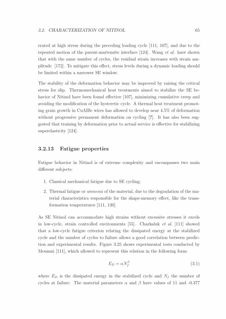
3.2. CHARACTERIZATION OF NITINOL 65
erated at high stress during the preceding loading cycle [111, 107], and due to the
repeated motion of the parent-martensite interface [124]. Wang et al. have shown
that with the same number of cycles, the residual strain increases with strain am-
plitude [172]. To mitigate this effect, stress levels during a dynamic loading should
be limited within a narrower SE window.
The stability of the deformation behavior may be improved by raising the critical
stress for slip. Thermomechanical heat treatments aimed to stabilize the SE be-
havior of Nitinol have been found effective [107], minimizing cumulative creep and
avoiding the modification of the hysteretic cycle. A thermal heat treatment promot-
ing grain growth in CuAlBe wires has allowed to develop near 4.5% of deformation
without progressive permanent deformation on cycling [?]. It has also been sug-
gested that training by deformation prior to actual service is effective for stabilizing
superelasticity [124].
3.2.13 Fatigue properties
Fatigue behavior in Nitinol is of extreme complexity and encompasses two main
different subjects:
1. Classical mechanical fatigue due to SE cycling;
2. Thermal fatigue or amnesia of the material, due to the degradation of the ma-
terial characteristics responsible for the shape-memory effect, like the trans-
formation temperatures [111, 130].
As SE Nitinol can accommodate high strains without excessive stresses it excels
in low-cycle, strain controlled environments [55]. Charkaluk et al. [111] showed
that a low-cycle fatigue criterion relating the dissipated energy at the stabilized
cycle and the number of cycles to failure allows a good correlation between predic-
tion and experimental results. Figure 3.25 shows experimental tests conducted by
Moumni [111], which allowed to represent this relation in the following form:
ED = αNβf (3.1)
where ED is the dissipated energy in the stabilized cycle and Nf the number of
cycles at failure. The material parameters α and β have values of 11 and -0.377
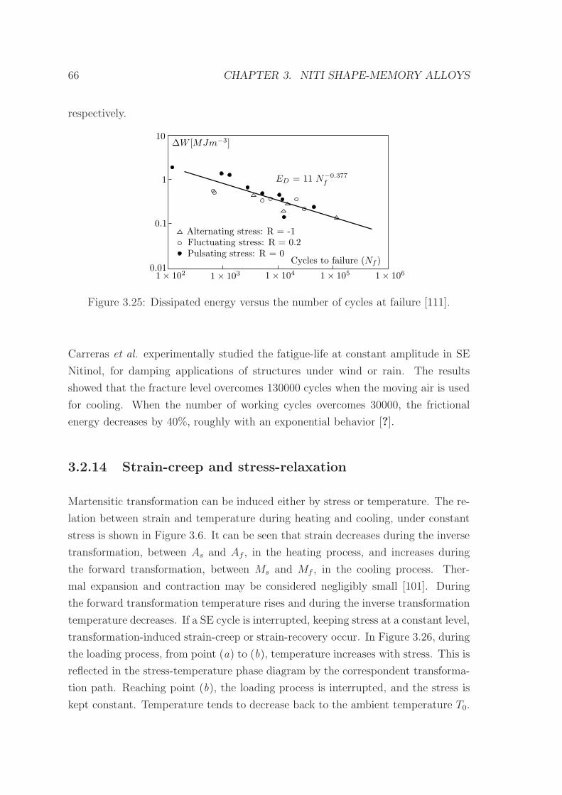
66 CHAPTER 3. NITI SHAPE-MEMORY ALLOYS
respectively.
∆W [MJm−3]
1
0.1
Fluctuating stress: R = 0.2Pulsating stress: R = 0
Alternating stress: R = -1
0.01Cycles to failure (Nf )
1× 10² 1× 10³ 1× 10⁴ 1× 10⁵ 1× 10⁶
ED = 11 N−0.377f
10
Figure 3.25: Dissipated energy versus the number of cycles at failure [111].
Carreras et al. experimentally studied the fatigue-life at constant amplitude in SE
Nitinol, for damping applications of structures under wind or rain. The results
showed that the fracture level overcomes 130000 cycles when the moving air is used
for cooling. When the number of working cycles overcomes 30000, the frictional
energy decreases by 40%, roughly with an exponential behavior [?].
3.2.14 Strain-creep and stress-relaxation
Martensitic transformation can be induced either by stress or temperature. The re-
lation between strain and temperature during heating and cooling, under constant
stress is shown in Figure 3.6. It can be seen that strain decreases during the inverse
transformation, between As and Af , in the heating process, and increases during
the forward transformation, between Ms and Mf , in the cooling process. Ther-
mal expansion and contraction may be considered negligibly small [101]. During
the forward transformation temperature rises and during the inverse transformation
temperature decreases. If a SE cycle is interrupted, keeping stress at a constant level,
transformation-induced strain-creep or strain-recovery occur. In Figure 3.26, during
the loading process, from point (a) to (b), temperature increases with stress. This is
reflected in the stress-temperature phase diagram by the correspondent transforma-
tion path. Reaching point (b), the loading process is interrupted, and the stress is
kept constant. Temperature tends to decrease back to the ambient temperature T0.
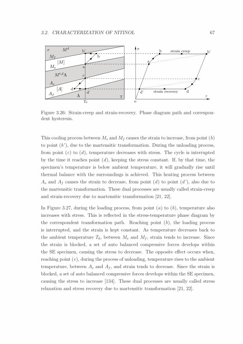
3.2. CHARACTERIZATION OF NITINOL 67
o
a
b’b
c
d’ d
b
c
a
dd’
b’
ε
σ
T
σ
T0
strain recovery
strain creepMd
A
[M ]
M t,dA
[A]
Mf
Ms
As
Af
Figure 3.26: Strain-creep and strain-recovery. Phase diagram path and correspon-dent hysteresis.
This cooling process betweenMs andMf causes the strain to increase, from point (b)
to point (b’ ), due to the martensitic transformation. During the unloading process,
from point (c) to (d), temperature decreases with stress. The cycle is interrupted
by the time it reaches point (d), keeping the stress constant. If, by that time, the
specimen’s temperature is below ambient temperature, it will gradually rise until
thermal balance with the surroundings is achieved. This heating process between
As and Af causes the strain to decrease, from point (d) to point (d’ ), also due to
the martensitic transformation. These dual processes are usually called strain-creep
and strain-recovery due to martensitic transformation [21, 22].
In Figure 3.27, during the loading process, from point (a) to (b), temperature also
increases with stress. This is reflected in the stress-temperature phase diagram by
the correspondent transformation path. Reaching point (b), the loading process
is interrupted, and the strain is kept constant. As temperature decreases back to
the ambient temperature T0, between Ms and Mf , strain tends to increase. Since
the strain is blocked, a set of auto balanced compressive forces develops within
the SE specimen, causing the stress to decrease. The opposite effect occurs when,
reaching point (e), during the process of unloading, temperature rises to the ambient
temperature, between As and Af , and strain tends to decrease. Since the strain is
blocked, a set of auto balanced compressive forces develops within the SE specimen,
causing the stress to increase [134]. These dual processes are usually called stress
relaxation and stress recovery due to martensitic transformation [21, 22].
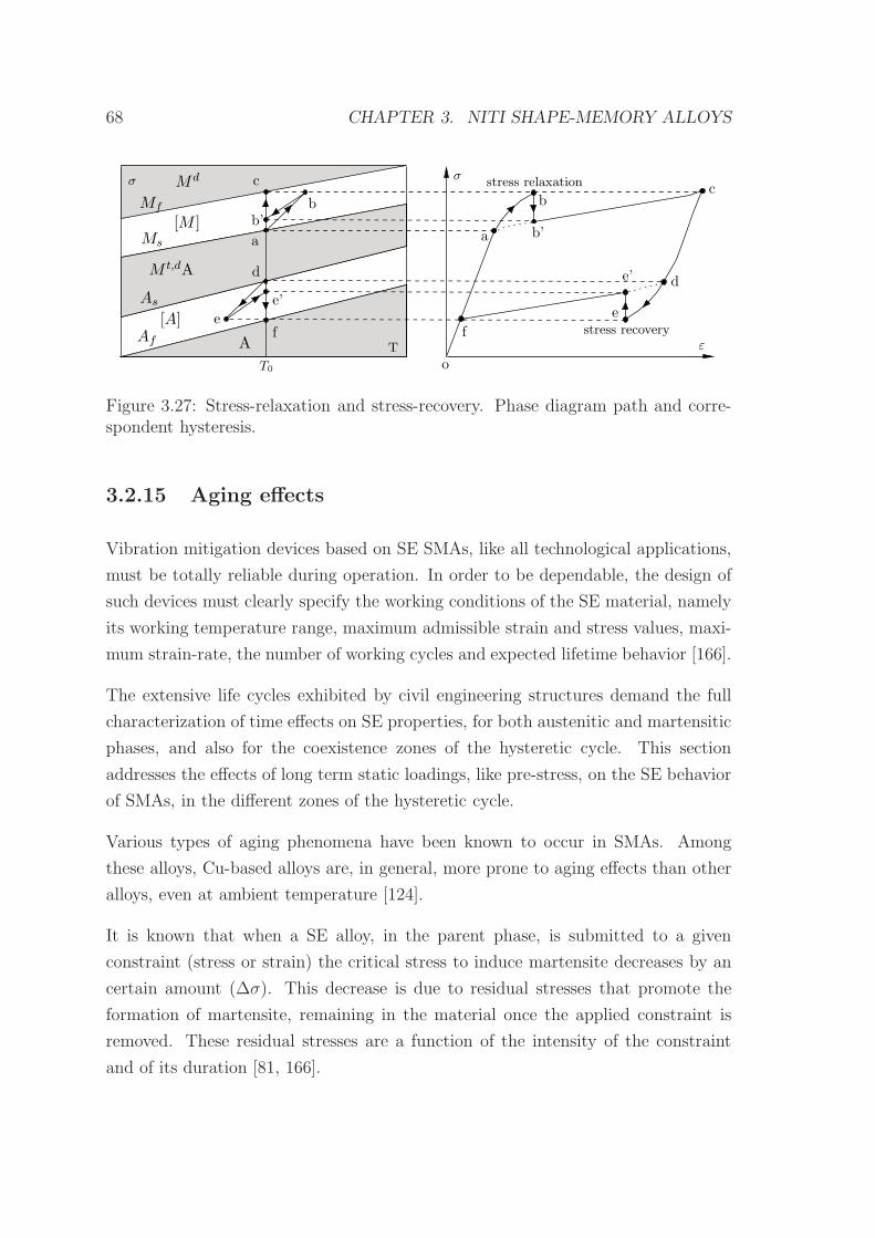
68 CHAPTER 3. NITI SHAPE-MEMORY ALLOYS
o
ab’
e’
b
e
c
a
d
f f
d
c
e’
ε
σ
T
σ
e
T0
b’
b
stress relaxation
stress recovery
Md
M t,dA
A
[M ]
[A]
Mf
Ms
As
Af
Figure 3.27: Stress-relaxation and stress-recovery. Phase diagram path and corre-spondent hysteresis.
3.2.15 Aging effects
Vibration mitigation devices based on SE SMAs, like all technological applications,
must be totally reliable during operation. In order to be dependable, the design of
such devices must clearly specify the working conditions of the SE material, namely
its working temperature range, maximum admissible strain and stress values, maxi-
mum strain-rate, the number of working cycles and expected lifetime behavior [166].
The extensive life cycles exhibited by civil engineering structures demand the full
characterization of time effects on SE properties, for both austenitic and martensitic
phases, and also for the coexistence zones of the hysteretic cycle. This section
addresses the effects of long term static loadings, like pre-stress, on the SE behavior
of SMAs, in the different zones of the hysteretic cycle.
Various types of aging phenomena have been known to occur in SMAs. Among
these alloys, Cu-based alloys are, in general, more prone to aging effects than other
alloys, even at ambient temperature [124].
It is known that when a SE alloy, in the parent phase, is submitted to a given
constraint (stress or strain) the critical stress to induce martensite decreases by an
certain amount (∆σ). This decrease is due to residual stresses that promote the
formation of martensite, remaining in the material once the applied constraint is
removed. These residual stresses are a function of the intensity of the constraint
and of its duration [81, 166].
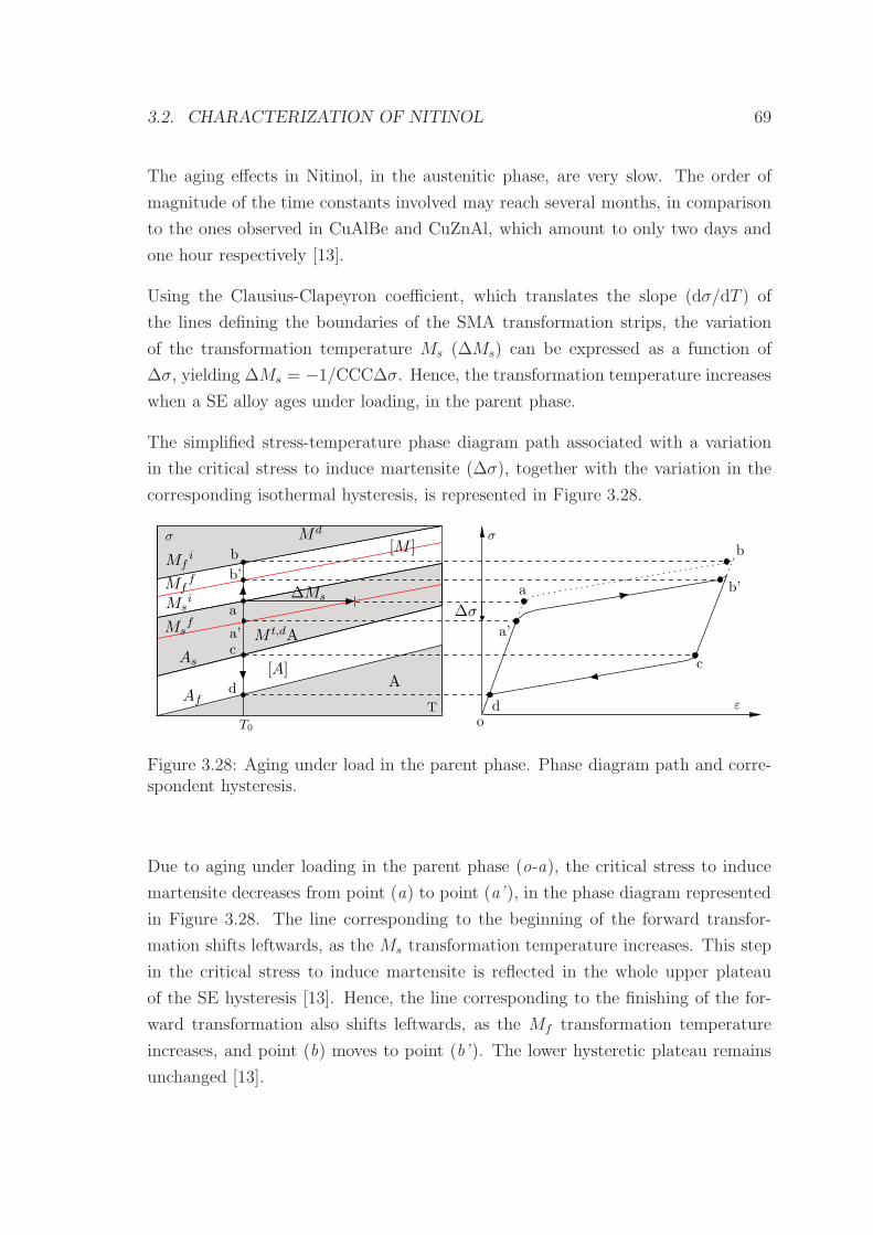
3.2. CHARACTERIZATION OF NITINOL 69
The aging effects in Nitinol, in the austenitic phase, are very slow. The order of
magnitude of the time constants involved may reach several months, in comparison
to the ones observed in CuAlBe and CuZnAl, which amount to only two days and
one hour respectively [13].
Using the Clausius-Clapeyron coefficient, which translates the slope (dσ/dT ) of
the lines defining the boundaries of the SMA transformation strips, the variation
of the transformation temperature Ms (∆Ms) can be expressed as a function of
∆σ, yielding ∆Ms = −1/CCC∆σ. Hence, the transformation temperature increases
when a SE alloy ages under loading, in the parent phase.
The simplified stress-temperature phase diagram path associated with a variation
in the critical stress to induce martensite (∆σ), together with the variation in the
corresponding isothermal hysteresis, is represented in Figure 3.28.
ε
σ
T
σ
o
a
a’
b
b’
c
d
A
b’
b
a’c
a
d
∆Ms
Md
[M ]
M t,dA
[A]
T0
As
Af
Mfi
Mff
Msi
∆σMs
f
Figure 3.28: Aging under load in the parent phase. Phase diagram path and corre-spondent hysteresis.
Due to aging under loading in the parent phase (o-a), the critical stress to induce
martensite decreases from point (a) to point (a’ ), in the phase diagram represented
in Figure 3.28. The line corresponding to the beginning of the forward transfor-
mation shifts leftwards, as the Ms transformation temperature increases. This step
in the critical stress to induce martensite is reflected in the whole upper plateau
of the SE hysteresis [13]. Hence, the line corresponding to the finishing of the for-
ward transformation also shifts leftwards, as the Mf transformation temperature
increases, and point (b) moves to point (b’ ). The lower hysteretic plateau remains
unchanged [13].
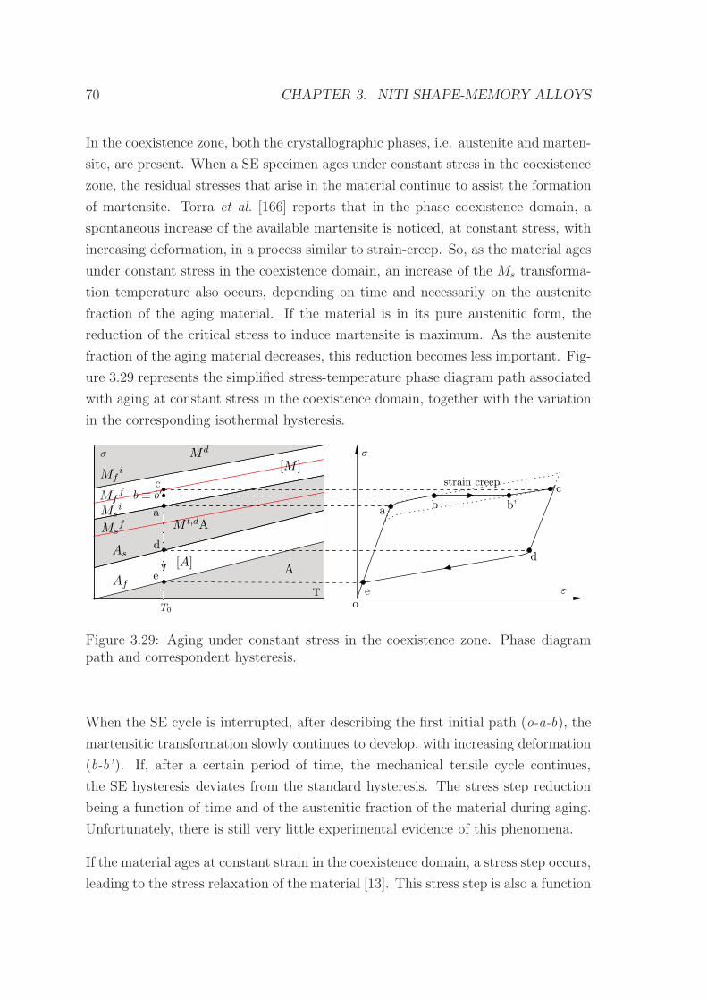
70 CHAPTER 3. NITI SHAPE-MEMORY ALLOYS
In the coexistence zone, both the crystallographic phases, i.e. austenite and marten-
site, are present. When a SE specimen ages under constant stress in the coexistence
zone, the residual stresses that arise in the material continue to assist the formation
of martensite. Torra et al. [166] reports that in the phase coexistence domain, a
spontaneous increase of the available martensite is noticed, at constant stress, with
increasing deformation, in a process similar to strain-creep. So, as the material ages
under constant stress in the coexistence domain, an increase of the Ms transforma-
tion temperature also occurs, depending on time and necessarily on the austenite
fraction of the aging material. If the material is in its pure austenitic form, the
reduction of the critical stress to induce martensite is maximum. As the austenite
fraction of the aging material decreases, this reduction becomes less important. Fig-
ure 3.29 represents the simplified stress-temperature phase diagram path associated
with aging at constant stress in the coexistence domain, together with the variation
in the corresponding isothermal hysteresis.
ε
σ
T
σ
o
a b b’
d
e
A
cstrain creepc
b ≡ b′
a
d
e
Md
[M ]
[A]
M t,dA
As
Af
T0
Mff
Msi
Msf
Mfi
Figure 3.29: Aging under constant stress in the coexistence zone. Phase diagrampath and correspondent hysteresis.
When the SE cycle is interrupted, after describing the first initial path (o-a-b), the
martensitic transformation slowly continues to develop, with increasing deformation
(b-b’ ). If, after a certain period of time, the mechanical tensile cycle continues,
the SE hysteresis deviates from the standard hysteresis. The stress step reduction
being a function of time and of the austenitic fraction of the material during aging.
Unfortunately, there is still very little experimental evidence of this phenomena.
If the material ages at constant strain in the coexistence domain, a stress step occurs,
leading to the stress relaxation of the material [13]. This stress step is also a function
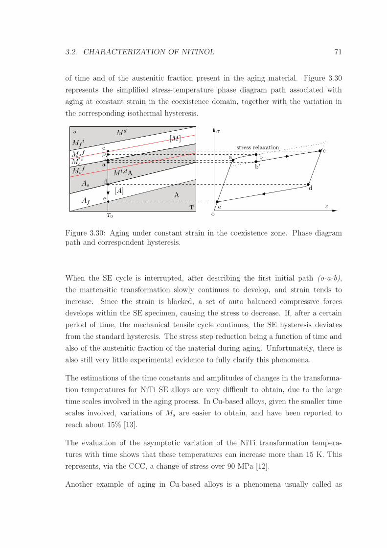
3.2. CHARACTERIZATION OF NITINOL 71
of time and of the austenitic fraction present in the aging material. Figure 3.30
represents the simplified stress-temperature phase diagram path associated with
aging at constant strain in the coexistence domain, together with the variation in
the corresponding isothermal hysteresis.
ε
σ
T
σ
o
d
e
d
eA
c
[M ]Md
b
stress relaxation
b’
c
ab’b
a
As
Af
[A]
T0
M t,dA
Mff
Msi
Msf
Mfi
Figure 3.30: Aging under constant strain in the coexistence zone. Phase diagrampath and correspondent hysteresis.
When the SE cycle is interrupted, after describing the first initial path (o-a-b),
the martensitic transformation slowly continues to develop, and strain tends to
increase. Since the strain is blocked, a set of auto balanced compressive forces
develops within the SE specimen, causing the stress to decrease. If, after a certain
period of time, the mechanical tensile cycle continues, the SE hysteresis deviates
from the standard hysteresis. The stress step reduction being a function of time and
also of the austenitic fraction of the material during aging. Unfortunately, there is
also still very little experimental evidence to fully clarify this phenomena.
The estimations of the time constants and amplitudes of changes in the transforma-
tion temperatures for NiTi SE alloys are very difficult to obtain, due to the large
time scales involved in the aging process. In Cu-based alloys, given the smaller time
scales involved, variations of Ms are easier to obtain, and have been reported to
reach about 15% [13].
The evaluation of the asymptotic variation of the NiTi transformation tempera-
tures with time shows that these temperatures can increase more than 15 K. This
represents, via the CCC, a change of stress over 90 MPa [12].
Another example of aging in Cu-based alloys is a phenomena usually called as
72 CHAPTER 3. NITI SHAPE-MEMORY ALLOYS
martensite stabilization. It consists in the gradual increase of the As temperature
with time, when aging in the martensite phase. The increase in As becomes more
important as temperature rises and may even cause the inhibition of the inverse
transformation [124].
3.3 Closure
Due to its outstanding fatigue properties, high corrosion resistance and ductility, the
majority of the SMA based industrial applications are mostly built up of Nitinol.
A microstructural survey of Nitinol allowed for the lattice characterization of its
bcc austenitic (B2) and monoclinic martensitic (B19’) crystal structures, as well
as to introduce the so-called R-phase, a trigonal phase associated with a two step
transformation from B2 to B19’.
In order to assess the tensile properties of Nitinol, uniaxial tensile tests are performed
on two wire specimens. These tensile tests enable the characterization of the loading
and unloading plateaus of the SE hysteretic cycles, associated with the forward and
inverse transformations, respectively. The austenitic and martensitic modulus of
elasticity (EA and EM) are also characterized, as well as the ultimate tensile strength
(σu) and elongation at failure.
Differential Scanning Calorimetry (DSC) is used to characterize the transformation
temperatures of a Nitinol wire specimen (Mf , Ms, As and Af). This thermoan-
alytical technique is based on the evaluation of the enthalpy of the martensitic
transformation during phase transition.
An experimental procedure to determine Clausius-Clapeyron coefficient (CCC) of a
previously stabilized Nitinol specimen is implemented, evaluating its critical trans-
formation stresses for a set of different ambient temperatures. The analysis of the
resulting SE hysteresis shows a clear temperature dependence, as the hysteretic
loop is shifted upwards with the rising of the ambient temperature. The stress-
temperature phase diagram associated with a temperature variation helps to clarify
this aspect. The equivalent viscous damping is computed for the obtained SE hys-
teresis, allowing to establish that an increase on the ambient temperature causes
the damping capacity of the Nitinol wire to decrease in a marginal way.
3.3. CLOSURE 73
The behavior of a SE Nitinol sample subjected to internal loops, i.e. to cycling
situations where the full extent of the forward and inverse transformations are not
attained is evaluated. A study regarding the influence of strain-amplitude on the
damping capacities of Nitinol is performed, based on the analysis of the stress-
temperature phase diagram path associated with a variation in the strain-amplitude,
and on tensile tests of increasing amplitude. The results show that as the marten-
sitic transformation begins, the damping capacity of the wire rapidly increases with
strain. After this first transitional phase, during the remaining extent of the marten-
sitic transformation, the damping capacity of the wire linearly increases with the
strain-amplitude.
To illustrate how the strain-rate of the dynamic loading may influence the temper-
ature variation of a SE specimen during a cyclic test, as well as the shape of its
corresponding hysteretic loop, a series of experimental tensile tests are conducted.
According to the results, for the range of tested strain-rates, when passing from
quasi-static conditions to dynamic ones, important changes occur, affecting the dis-
sipation capability of the SMA wire. The computation of the equivalent viscous
damping demonstrates that, as the strain-rate increased, the dissipation capacity of
the Nitinol wire initially increased and then started to decrease.
An experimental setup is built in order to observe the propagation of the transfor-
mation fronts that accompany the phase transitions during the uniaxial loading of
SMAs. The results show that during the loading process the propagating transfor-
mation fronts start from the central part of the specimen and develop towards the
specimen grips. During the unloading process, they move the opposite way, from
the grips and towards the central part of the specimen.
An experimental study to clarify some of the implications of cyclic loading on the SE
stress-strain diagram is performed. This study is based on the analysis of the evo-
lution of the stress-strain diagram of a Nitinol wire specimen during cyclic loading.
The cumulative creep deformation, the critical stress needed to induce martensite
and the width of the hysteretic loop are quantified, under different cyclic loading
conditions regarding ambient temperature and strain-rate, and although the effects
under consideration are proved rather important, they gradually disappear with
cycling. It is also shown that degradation increases with both temperature and
strain-rate. Since cumulative creep in Nitinol is mainly due to lattice defects gen-
erated at high stress, one way to limit this effect is to keep the stress levels during

74 CHAPTER 3. NITI SHAPE-MEMORY ALLOYS
dynamic loading within a narrower SE window, also reducing the influence of cycling
on damping.
It is shown that due to temperature variation during a non-isothermal SE cycle, if
a SE cycle is interrupted, keeping stress at a constant level, transformation-induced
strain-creep or strain-recovery occur in Nitinol. Stress-relaxation and stress-recovery
due to martensitic transformation are also addressed. Regarding the Nitinol aging
effects it is shown that if the material ages at constant strain in the coexistence
domain, a stress step occurs, leading to the stress relaxation of the material.
Chapter 4
Constitutive Models for
Shape-Memory Alloys
4.1 Introduction
The behavior of SMAs shows a high level of complexity, since it depends on stress
and temperature, and is closely connected with the crystallographic phase of the
material and the thermodynamics underlying the transformation processes. For
this reason, any simulation regarding the design of a particular system that makes
use of the interesting features exhibited by these materials, has to be based on an
adequate constitutive model. The model must be able to conveniently cope with the
relevant set of SMA’s properties regarding the type of application at stake. While
rate-independent models, insensitive to the velocity of the applied strain or stress,
may be well suited for quasi-static analysis, when isothermal conditions are present,
for most dynamic applications, rate-dependent models are usually required, due to
self-heating.
Several constitutive mathematical models for SMAs are currently available in the
literature [16, 17, 18, 20, 26, 30, 31, 60, 63, 64, 65, 103, 128, 129, 155], most of them
being aimed at the one-dimensional description of the material behavior. One of
the common features present in most of them, is that they can be separated into
a mechanical law, governing the stress-strain behavior, and kinetic laws, governing
the transformation behavior. These two relations are often coupled [30]. Rate-
75
76 CHAPTER 4. CONSTITUTIVE MODELS FOR SMAS
dependent models require an additional thermal balance equation, coupled with the
mechanical and kinetic laws.
In this work, two different constitutive models are considered, a rate-independent
constitutive model, based on the model proposed by Auricchio [15, 60, 103], and a
rate-dependent constitutive model, based on the model proposed by Tanaka [159].
4.2 Mechanical laws
In a typical SMA constitutive model, the mechanical law relates stress (σ), strain
(ε), temperature (T ) and martensite fraction (ξ). Martensite fraction is an internal
state variable that represents the extent of the transformation in the material and
can be regarded as the fraction of the produced phase. The original phase occupies,
therefore, the rest, 1 - ξ.
The transformed phase fraction is considered to be in series with the elastic frac-
tion of the response. There are several approaches for mathematical modeling of
this elastic component. If the elastic fraction of the response is considered to be
limited to the austenite phase, the model represented in Figure 4.1(a) is obtained.
The models represented in Figure 4.1(b) and (c) contemplate two different crystal-
lographic phases, austenite and martensite, not distinguishing between the twinned
and the detwinned martensite. Considering a parallel distribution of austenite and
martensite within the material, equivalent to the Voight scheme, yields the model
represented in Figure 4.1(b). If, in alternative, the mechanical model is based in a
periodical distribution of austenite and martensite within the material, orthogonal
to the direction of the applied stress, the model represented in Figure 4.1(c), which
is equivalent to the Reuss scheme, is obtained.
4.2.1 Simple serial model
For the mechanical model expressed in Figure 4.1(a), as the principle of superposi-
tion applies, the total strain results from the sum of the elastic strain (εelast.) with
the transformation strain (εtransf.),
ε = εelast. + εtransf. (4.1)
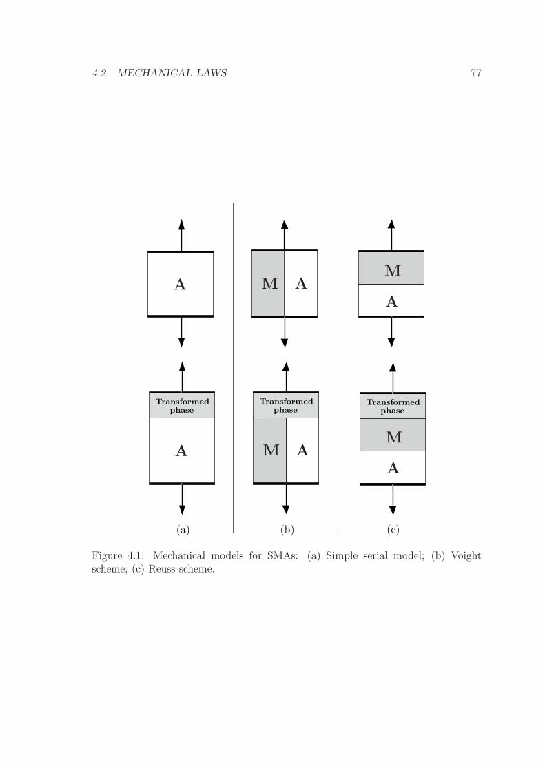
4.2. MECHANICAL LAWS 77
A
A M A
AM
M
A
M
A
(a) (b) (c)
Transformedphase phase
Transformedphase
Transformed
Figure 4.1: Mechanical models for SMAs: (a) Simple serial model; (b) Voightscheme; (c) Reuss scheme.
78 CHAPTER 4. CONSTITUTIVE MODELS FOR SMAS
The transformation strain can be written as
εtransf. = εLξ with 0 ≤ ξ ≤ 1 (4.2)
and
εelast. = ε− εLξ (4.3)
where εL is the maximum residual strain in the material. As the elastic strain equals
the austenitic strain (εelast. = εA), the total strain reads
ε = εA + εLξ (4.4)
and the mechanical law governing the stress-strain behavior yields
σ = σA = EAεA = EA(ε− εLξ) (4.5)
where EA is the austenitic elastic modulus. This model neglects the additional
thermal strain component, which is several orders of magnitude smaller than the
transformation strain [30].
4.2.2 Voight scheme
For the mechanical model equivalent to the the Voight scheme, in Figure 4.1(b), as
the elastic strain equals the austenitic and martensitic strains (εelast. = εA = εM),
the mechanical law governing the behavior of the material can be written as
σ = ξσM + (1− ξ)σA (4.6)
Taking into account that σA = EAεA and σM = EMεM , it yields
σ = [ξEM + (1− ξ)EA]εelast. = [ξEM + (1− ξ)EA](ε− εLξ) (4.7)
where εM is the martensitic strain, and EM the martensitic elastic modulus. Adding
the thermal strain component to equation(4.7) results in the mechanical law pro-
posed by Tanaka [159]
σ = [ξEM + (1− ξ)EA](ε− εLξ) + θ(T − T0) (4.8)
4.3. KINETIC LAWS 79
where θ is related to the thermal coefficient of expansion and T0 is the temperature
at which the thermal strain is defined to be zero [44].
4.2.3 Reuss scheme
For the mechanical model equivalent to the Reuss scheme, in Figure 4.1(c), the total
strain can be expressed as
ε = ξεM + (1− ξ)εA (4.9)
The stress in each phase is equal to the overall applied stress and the individual
phase strains are given by εA = σ/EA and εM = σ/EM + εL. Substituting the
austenite and martensite phase strains in (4.9) results that
σ =EAEM
ξEA + (1− ξ)EM(ε− εLξ) (4.10)
The Ishvin-Pence mechanical law [30] is obtained by adding the thermal strain com-
ponent to equation(4.10), yielding
σ =EAEM
ξEA + (1− ξ)EM
(ε− εLξ) + θ(T − T0) (4.11)
4.3 Kinetic laws
In order to complete the constitutive model, the mechanical law must be coupled
with the transformation kinetic equations. These expressions describe mathemat-
ically the evolution of the martensite fraction with stress and temperature, based
on the material’s stress-temperature phase diagram. There are several kinetic laws
available in the literature. They range from the linear kinetic laws proposed by Au-
richio [15], the exponential laws proposed by Tanaka [159, 160], to the cosine based
kinetic laws proposed by Liang and Rogers [96] and to thermodynamically derived
relations, proposed by Ishvin and Pence [79]. In the present work only the linear
and the exponential kinetic relations were used.
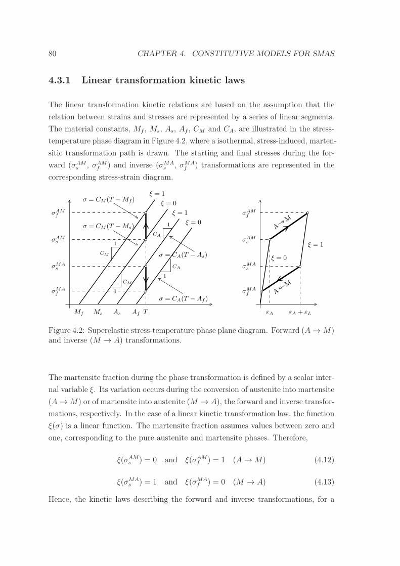
80 CHAPTER 4. CONSTITUTIVE MODELS FOR SMAS
4.3.1 Linear transformation kinetic laws
The linear transformation kinetic relations are based on the assumption that the
relation between strains and stresses are represented by a series of linear segments.
The material constants, Mf , Ms, As, Af , CM and CA, are illustrated in the stress-
temperature phase diagram in Figure 4.2, where a isothermal, stress-induced, marten-
sitic transformation path is drawn. The starting and final stresses during the for-
ward (σAMs , σAM
f ) and inverse (σMAs , σMA
f ) transformations are represented in the
corresponding stress-strain diagram.
AM
Mf Ms As Af T
σAMf
σAMs
σMAf
1
CM
CM
1
ξ = 1
ξ = 0
ξ = 1
ξ = 0
CA
1
1
CA
σ = CM (T −Ms)
σ = CM (T −Mf)
σ = CA(T −As)
σAMf
σAMs
σMAs σMA
s
σMAf
ξ = 0
ξ = 1
εA + εLεA
AM
σ = CA(T −Af )
Figure 4.2: Superelastic stress-temperature phase plane diagram. Forward (A→ M)and inverse (M → A) transformations.
The martensite fraction during the phase transformation is defined by a scalar inter-
nal variable ξ. Its variation occurs during the conversion of austenite into martensite
(A→M) or of martensite into austenite (M → A), the forward and inverse transfor-
mations, respectively. In the case of a linear kinetic transformation law, the function
ξ(σ) is a linear function. The martensite fraction assumes values between zero and
one, corresponding to the pure austenite and martensite phases. Therefore,
ξ(σAMs ) = 0 and ξ(σAM
f ) = 1 (A→M) (4.12)
ξ(σMAs ) = 1 and ξ(σMA
f ) = 0 (M → A) (4.13)
Hence, the kinetic laws describing the forward and inverse transformations, for a
4.3. KINETIC LAWS 81
specific temperature (T ), may be written as,
ξAM =σ − σAM
s
σAMf − σAM
s
(4.14)
ξMA =σ − σMA
f
σMAs − σMA
f
(4.15)
Using the equations that define the boundary lines of the transformation strips,
represented in the left hand graph of Figure 4.2,
σAMs = CM(T −Ms) and σAM
f = CM(T −Mf ) (4.16)
σMAs = CA(T − As) and σAM
f = CA(T − Af) (4.17)
the kinetic laws describing the transformations may be generalized for any given
temperature, yielding, for the forward and inverse transformations,
ξAM =σ − CM(T −Ms)
CM(Ms −Mf )(4.18)
ξMA =σ − CA(T − Af)
CA(Af − As)(4.19)
4.3.2 Exponential transformation kinetic laws
The Tanaka’s exponential laws are based in the Magee’s transformation kinetics
equations, originally proposed for steels [?, 100]. For the forward and inverse trans-
formations, they yield,
ξ
1− ξ= aM T − bM σ (A→ M) (4.20)
and
−ξ
ξ= aAT − bAσ (M → A) (4.21)
Let one consider a forward transformation process starting from the initial values
(σ0, T0, ξ0), where ξ0 stands for the fraction of martensite at the start of the forward
transformation. If the transformation kinetics (4.20) is integrated from the initial
values to the current values (σ, T , ξ), for constant material parameters aM and bM ,
82 CHAPTER 4. CONSTITUTIVE MODELS FOR SMAS
one finally obtains an explicit form of the forward transformation kinetics,
1− ξ = (1− ξ0) exp [−aM (T − T0) + bM(σ − σ0)]
since ξ0 = 0 and σ0 = CM(T0 −Ms),
ξ = 1− exp−aM(T − T0) + bM [σ − CM(T0 −Ms)]
and taking into account that bMCM = aM ,
ξAM = 1− exp [aM (Ms − T ) + bMσ] (4.22)
where Ms is the temperature at which the forward transformation starts, in the
stress-free state. This equation is valid if σ > CM(T −Ms).
Now, consider a inverse transformation process, starting from the initial values (σ0,
T0, ξ0), where ξ0 stands for the fraction of martensite at the start of the inverse
transformation. If the transformation kinetics (4.21) is integrated from the initial
values to the current values (σ, T , ξ), for constant material parameters aM and bM ,
one finally obtains an explicit form of the inverse transformation kinetics,
ξ = ξ0 exp[−aA(T − T0) + bA(σ − σ0)]
since ξ0 = 1 and σ0 = CA(T0 −As),
ξ = exp −aA(T − T0) + bA[σ − CA(T0 −As)]
and taking into account that bACA = aA,
ξMA = exp[aA(As − T ) + bAσ] (4.23)
where As is the temperature at which the inverse transformation starts, in the stress-
free state. This equation is valid if σ ≤ CA(T −As).
The exponential law equations (4.22) and (4.23) are well known in the literature
and widely used [169].
To determine the material constants aM , bM , one follows the usual understand-
ing in metallurgy [10], assuming that the forward transformation is complete when
4.4. THERMAL EFFECTS 83
ξ = 0.99. This results in,
ξAM = 1− exp [aM (Ms − T ) + bMσ]
0.99 = 1− exp [aM(Ms − T ) + bMCM(T −Mf )]
aM = −2 ln 10
Ms −Mf
, bM =aMCM
(A→M) (4.24)
The material constants aA and bA are calculated similarly, assuming that the com-
pletion of the inverse transformation occurs when ξ = 0.01
ξMA = exp[aA(As − T ) + bAσ]
0.01 = exp[aA(As − T ) + bACA(T −Af )]
aA =2 ln 10
Af − As, bA =
aACA
(M → A) (4.25)
4.4 Thermal effects
Although the heat exchanges between the SE material and its surrounding environ-
ment generates almost isothermic processes, when quasi-static loading conditions
are present, as the rate of the dynamic loading increases, the total amount of gener-
ated energy per unit time increases accordingly. For fast dynamic cycling, since the
dissipation capacity of the thermo-mechanical system is limited by the heat con-
vection mechanism, the generated and the dissipated energy become unbalanced,
causing the specimen’s temperature to change, as well as the shape of the hysteretic
loop. For a SMA constitutive model to conveniently apprehend this phenomena,
it is necessary to couple, together with the mechanical and kinetic transformation
laws, an adequate heat balance equation. In this section, the heat transfer problem
is addressed.
The heat transfer system, as illustrated in Figure 4.3, consists of a cylindrical Nitinol
wire with a circular cross section, fixed at both extremities and surrounded by air,
at temperature Tf . There are internal energy sources, within the wire, deriving
from the enthalpy of the martensitic transformations and internal friction, both
occurring during a hysteretic SE cycle. It is assumed that the heat conduction
through the wire’s extremities is negligible. The differential formulation for the
problem of temperature distribution in a cylinder with uniform heat generation is
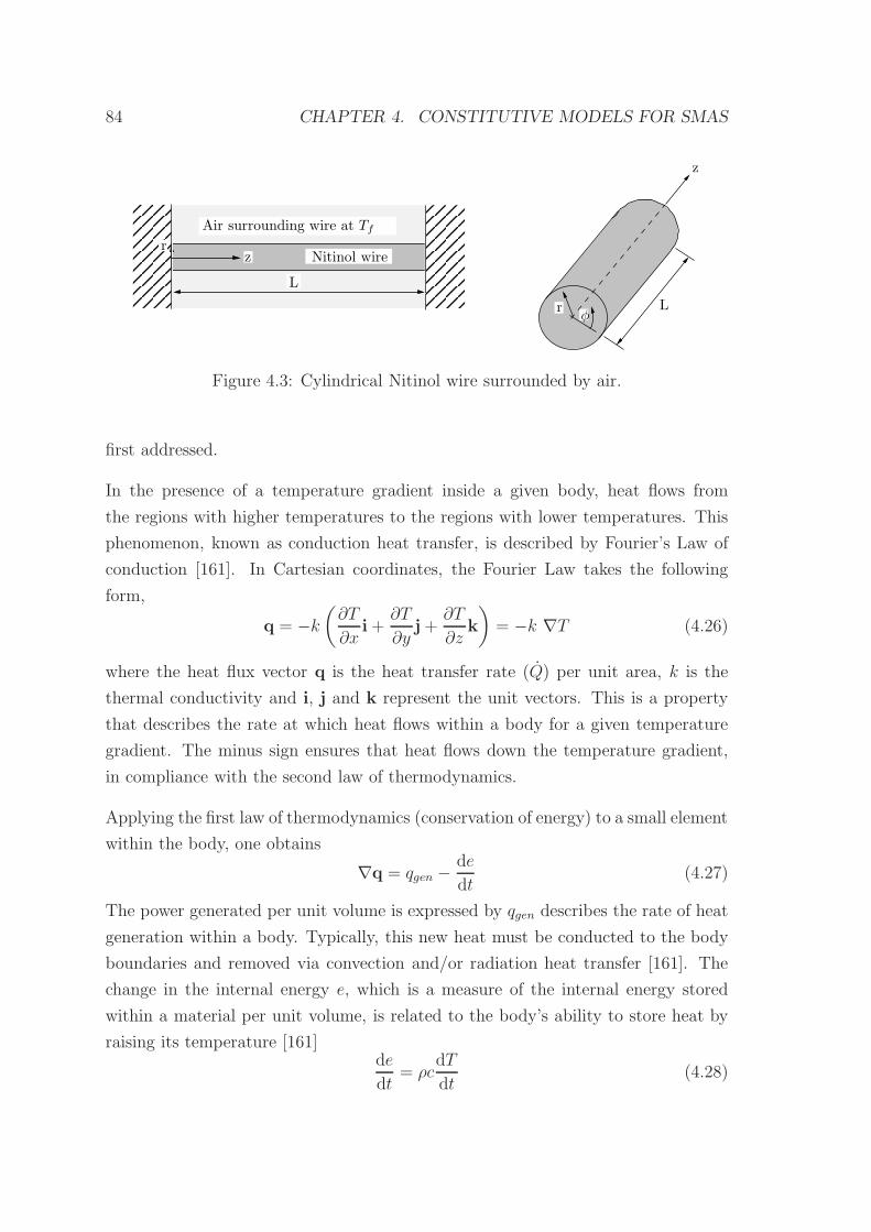
84 CHAPTER 4. CONSTITUTIVE MODELS FOR SMAS
Air surrounding wire at Tf
Nitinol wirer
z
L
rφ
L
z
Figure 4.3: Cylindrical Nitinol wire surrounded by air.
first addressed.
In the presence of a temperature gradient inside a given body, heat flows from
the regions with higher temperatures to the regions with lower temperatures. This
phenomenon, known as conduction heat transfer, is described by Fourier’s Law of
conduction [161]. In Cartesian coordinates, the Fourier Law takes the following
form,
q = −k
(
∂T
∂xi+
∂T
∂yj+
∂T
∂zk
)
= −k ∇T (4.26)
where the heat flux vector q is the heat transfer rate (Q) per unit area, k is the
thermal conductivity and i, j and k represent the unit vectors. This is a property
that describes the rate at which heat flows within a body for a given temperature
gradient. The minus sign ensures that heat flows down the temperature gradient,
in compliance with the second law of thermodynamics.
Applying the first law of thermodynamics (conservation of energy) to a small element
within the body, one obtains
∇q = qgen −de
dt(4.27)
The power generated per unit volume is expressed by qgen describes the rate of heat
generation within a body. Typically, this new heat must be conducted to the body
boundaries and removed via convection and/or radiation heat transfer [161]. The
change in the internal energy e, which is a measure of the internal energy stored
within a material per unit volume, is related to the body’s ability to store heat by
raising its temperature [161]de
dt= ρc
dT
dt(4.28)
4.4. THERMAL EFFECTS 85
In the above relation, ρ is the density of the material and c its specific heat, a
material property that indicates the amount of energy a body stores for each degree
increase in temperature, on a per unit mass basis.
The energy equation may be obtained substituting the Fourier’s Law of heat con-
duction in equation (4.27) and using definition (4.28) for the change in the internal
energy,
∇2 T −ρc
k
dT
dt= −
qgenk
(4.29)
It can be concluded that the temperature profile within a body depends upon the
rate of its internally-generated heat, its capacity to store some of this heat, and its
rate of thermal conduction to its boundaries [161].
The energy equation (4.29) can be rewritten using cylindrical coordinates; see Fig-
ure 4.3, as:
1
r
∂
∂r
(
r∂T
∂r
)
+1
r2∂2T
∂φ2+∂2T
∂z2−ρc
k
∂T
∂t= −
qgenk, T = T (r, φ, z, t) (4.30)
Since the cylindrical Nitinol wire is surrounded by air, the heat transfer mechanism
is called convection. In convection, the conduction heat transfer mechanism always
plays a primary role. Regarding the mechanisms in which fluid motion is produced,
convection systems are characterized in forced convection and natural convection.
While natural convection is caused by temperature-induced density gradients within
the fluid, forced convection involves fluid motion caused by mechanical means, such
as pumps and fans [76].
A practical approach to the analysis of convection heat transfer from surfaces has
been developed in [161], which employs an equation of the form,
qc = hAs(Ts − Tf ) (4.31)
where qc is the heat flux transferred from a surface at uniform temperature Ts to
a fluid with reference temperature Tf , As is the surface area and h is the mean
coefficient of heat transfer. Equation (4.31) is usually referred to as the Newton law
of cooling [161].
In convection, the mean coefficient of heat transfer replaces the role of the ther-
mal conductivity that appears in conduction heat transfer, present in the Fourier’s
86 CHAPTER 4. CONSTITUTIVE MODELS FOR SMAS
Law (4.26). The mean coefficient of heat transfer depends upon the hydrodynamic
conditions as well as on the thermodynamic and thermophysical properties of the
fluid.
In some cases, for particular values of the Biot number, the energy equation (4.30)
can be further simplified. The Biot number (Bi) is defined as
Bi =hLc
k(4.32)
where Lc is the characteristic length, commonly defined as the volume of the body
divided by the surface area of the body, such that Lc = Vb/As. The Biot number is
a dimensionless number that gives a simple index of the ratio of the heat transfer
resistances inside and at the surface of a body. This ratio determines whether or
not the temperatures inside a body will vary significantly in space, while the body
heats or cools over time [76]. For small values of the Biot number, the variation
of temperature within the cylindrical Nitinol wire is essentially independent of r .
Values of the Biot number less than 0.1 imply that the heat conduction inside the
body is much faster than the heat convection away from its surface, and temperature
gradients are negligible inside of it. In these cases, the use of an one-dimensional
analysis leads to an error less than about 10% [161]. According to [76], the energy
equation expressed in (4.30), can be thus simplified to the following form,
−ρcVdT
dt= hA [T − Tf ]− qgenV with T (0) = Tf (4.33)
The power generated per unit volume, is described by,
qgen = cLρdξ
dt+
dW
dt(4.34)
The first term is related to the martensite fraction, assuming constant latent heat of
transformation, cL, and the second term to internal friction. In a complete tensile
loading-unloading cycle, the dissipated energy by internal friction corresponds to the
total area enclosed by the hysteretic cycle. The total generated power during this
cycle may, therefore, be computed by dividing the dissipated energy by the duration
of the cycle.
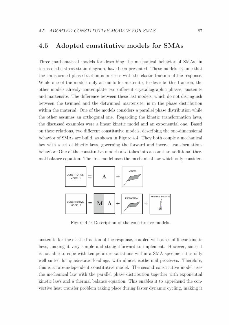
4.5. ADOPTED CONSTITUTIVE MODELS FOR SMAS 87
4.5 Adopted constitutive models for SMAs
Three mathematical models for describing the mechanical behavior of SMAs, in
terms of the stress-strain diagram, have been presented. These models assume that
the transformed phase fraction is in series with the elastic fraction of the response.
While one of the models only accounts for austenite, to describe this fraction, the
other models already contemplate two different crystallographic phases, austenite
and martensite. The difference between these last models, which do not distinguish
between the twinned and the detwinned martensite, is in the phase distribution
within the material. One of the models considers a parallel phase distribution while
the other assumes an orthogonal one. Regarding the kinetic transformation laws,
the discussed examples were a linear kinetic model and an exponential one. Based
on these relations, two different constitutive models, describing the one-dimensional
behavior of SMAs are build, as shown in Figure 4.4. They both couple a mechanical
law with a set of kinetic laws, governing the forward and inverse transformations
behavior. One of the constitutive models also takes into account an additional ther-
mal balance equation. The first model uses the mechanical law which only considers
MODEL 1
CONSTITUTIVE +
+ +
LINEAR
=
=CONSTITUTIVE
MODEL 2
THERMAL BALANCEEXPONENTIAL
AM
A
Figure 4.4: Description of the constitutive models.
austenite for the elastic fraction of the response, coupled with a set of linear kinetic
laws, making it very simple and straightforward to implement. However, since it
is not able to cope with temperature variations within a SMA specimen it is only
well suited for quasi-static loadings, with almost isothermal processes. Therefore,
this is a rate-independent constitutive model. The second constitutive model uses
the mechanical law with the parallel phase distribution together with exponential
kinetic laws and a thermal balance equation. This enables it to apprehend the con-
vective heat transfer problem taking place during faster dynamic cycling, making it
88 CHAPTER 4. CONSTITUTIVE MODELS FOR SMAS
a rate-dependent constitutive model.
4.6 Numerical implementation of the models
Having discussed the theoretical background concerning the two SMA constitutive
models, the numerical implementation of these models is now addressed. These
numerical implementations are based on strain-driven, time-discrete models, and
are aimed to simulate the SE behavior of SMA’s under uniaxial loadings. The
numerical algorithms are implemented in a Matlab R2007a environment.
4.6.1 Numerical implementation of the rate-independent con-
stitutive model
The rate-independent constitutive model is based on the assumption that the rela-
tion between strains and stresses is represented by a series of linear segments. The
material parameters characterizing the model are the austenitic elastic modulus
EA, the strain associated with the transformation process εL, the starting and final
stresses during the forward transformation, σAMs and σAM
f and the corresponding
stresses during the inverse transformation, σMAs and σMA
f . The linear kinetic laws
describing the forward and inverse transformations are defined as,
ξAM =σ − CM(T −Ms)
CM(Ms −Mf )with σAM
s < σ < σAMf and σ > 0
ξMA =σ − CA(T − Af)
CA(Af −As)with σMA
f < σ < σMAs and σ < 0
where ξ is a scalar internal variable representing the martensite fraction during the
phase transformation.
For a given temperature T , the starting and final stresses during the forward trans-
formation (σAMs , σAM
f ) may be computed using the equations that define the bound-
ary lines of the corresponding transformation strips. Assuming a time-continuous
model, the time evolution of the martensite fraction, is expressed using a stress-
driven linear kinetic rule to yield its corresponding evolution equation. For the
4.6. NUMERICAL IMPLEMENTATION OF THE MODELS 89
forward transformation one has,
ξAM =σ − σAM
s
σAMf − σAM
s
ξAM =σ
σAMf − σAM
s
= −(1− ξAM)σ
σ − σAMf
(4.35)
In the case of the inverse transformation, the martensite fraction and its evolution
equation reads,
ξMA =σ − σMA
f
σMAs − σMA
f
ξMA =σ
σMAs − σMA
f
= ξMA σ
σ − σMAf
(4.36)
On the other hand, stress and its evolution equation, for the mechanical law which
only considers austenite for the elastic fraction of the response (4.5), are defined as,
σ = EA(ε− εLξ) and σ = EA(ε− εLξ) (4.37)
Replacing σ, in the transformation kinetic relations expressed by equations (4.35)
and (4.36), it yields
ξAM =(1− ξAM)EAε
(1− ξAM)EAεL + σAMf − σ
(4.38)
and
ξMA =ξMAEAε
ξMAEAεL − σMAf + σ
(4.39)
for the forward and inverse transformations, respectively.
One wants to approximate the solution of the initial value problem
y = f(t, y), with y(t0) = y0 (4.40)
by using the first two terms of the Taylor expansion of y, representing the lin-
ear approximation around the point (t0, y(t0)). Defining the incremental quantity
90 CHAPTER 4. CONSTITUTIVE MODELS FOR SMAS
∆tn = tn+1 − tn, one may write
yn+1 = yn +∆tnf(tn, yn) (4.41)
This first-order numerical procedure for solving ordinary differential equations, with
a given initial value, is called the Euler method [9]. The Euler method is an example
of an explicit method, where yn+1 is defined by terms that are already known, like
yn. Let one define the additional incremental quantities,
ξn = ξn+1 − ξn, ∆εn = εn+1 − εn
∆Tn = Tn+1 − Tn and ∆Wn = Wn+1 −Wn (4.42)
The use of the Euler method enables the transformation of the time-continuous
evolutionary equations (4.38) and (4.39), into time-discrete evolutionary equations,
∆ξAMn =
(1− ξAM)EA∆εn(1− ξAM)EAεL + σAM
f − σ(4.43)
for the forward transformation time-discrete evolutionary equation, and
∆ξMAn =
ξMAEA∆εnξMAEAεL − σMA
f + σ(4.44)
for the inverse transformation time-discrete evolutionary equation.
Finally, it is possible to obtain the equations describing the evolution of the marten-
site fraction according to the strain history. In particular, for the conversion of
austenite into martensite one has,
ξAMn+1 = ξAM
n +(1− ξAM
n )EA(εn+1 − εn)
(1− ξAMn )EAεL + σAM
f − σn(4.45)
while for the conversion of martensite into austenite one has,
ξMAn+1 = ξMA
n +ξMAn EA(εn+1 − εn)
ξMAn EAεL − σMA
f + σn(4.46)
Note that, in the above equations, the subscripts n and n + 1 indicates quantities
4.6. NUMERICAL IMPLEMENTATION OF THE MODELS 91
evaluated at times tn and tn+1, respectively. Although the time-continuous model
is stress-driven, the time-discrete model assumes strain as the control variable. The
choice is consistent with the fact that, from the point of view of the integration
scheme, the time-discrete problem is considered strain-driven.
4.6.2 Algorithm for the rate-independent constitutive model
The implemented algorithm for the rate-independent (R-I) constitutive model is
presented next:
1. Initial calculations
(a) Define Tf (ambient temperature), ε (strain-rate) and ∆t
(b) For i = 0, initialize T0, ε0, σ0 and ξ0
2. Calculations for every time step, i
(a) Evaluate the strain increment by multiplying the strain-rate by the dis-
crete time parameter and update the strain,
εi+1 = εi + ε∆t
(b) Solve the system of equations formed by the constitutive and one of the
kinetic laws to obtain the martensite fraction and stress,
ξAMi+1 = ξAM
i +(1− ξAM
i )EA(εi+1 − εi)(1− ξAM
i )EAεL + σAMf − σi
σi+1 = EA(εi+1 − εLξAMi+1 )
for the forward transformation, and
ξMAi+1 = ξMA
i +ξMAi EA(εi+1 − εi)
ξMAi EAεL − σMA
f + σi
σi+1 = EA(εi+1 − εLξMAi+1 )
for the inverse transformation
92 CHAPTER 4. CONSTITUTIVE MODELS FOR SMAS
3. Repetition for the next time step. Replace i by i+ 1 and goto step 2, for the
next time step. Stop when reached the final time.
4.6.3 Numerical implementation of the rate-dependent con-
stitutive model
The exponential kinetic laws describing the forward and inverse transformations, for
the rate-dependent model, are defined by,
ξAM = (1− ξ)(aM T − bM σ) (4.47)
and
ξMA = ξ(−aAT + bAσ) (4.48)
Stress and its time-derivative, according to the mechanical law proposed by Tanaka,
expressed by equation (4.8), in which, without loss of generality, T0 is assumed to
be zero, read,
σ = [ξ(EM −EA) + EA](ε− εLξ) + θT
σ = E(ξ)ε+H(ξ)ξ + θT (4.49)
where
E(ξ) = ξ(EM − EA) + EA (4.50)
and
H(ξ) = (EM −EA)(ε− εLξ)− εLE(ξ) (4.51)
Replacing σ, in the transformation kinetic relations expressed in equations (4.47)
and (4.48), yields,
ξAM =(1− ξAM)[(aM − bMθ)T − bME(ξ)ε]
1 + (1− ξAM)bMH(ξ)(4.52)
for the forward transformation, and
ξMA =ξMA[(−aA + bAθ)T + bAE(ξ)ε]
1− ξMAbAH(ξ)(4.53)
4.6. NUMERICAL IMPLEMENTATION OF THE MODELS 93
for the inverse transformation. Reformulating equations (4.52) and (4.53), using
the definitions for the incremental quantities in (4.42), yields the increment of the
martensite fraction for the forward transformation,
∆ξAMn =
(1− ξAM)[(aM − bMθ)∆T − bME(ξ)∆ε]
1 + (1− ξAM)bMH(ξ)(4.54)
and the correspondent martensite fraction increment for the inverse transformation,
∆ξMAn =
ξMA[(−aA + bAθ)∆T + bAE(ξ)∆ε]
1− ξMAbAH(ξ)(4.55)
Hence, one can obtain the equations describing the evolution of the martensite
fraction according to the strain and temperature histories. In particular, for the
conversion of austenite into martensite one has,
ξAMn+1 = ξAM
n + (1− ξAMn )
[
(aM − bMθ)(Tn+1 − Tn)
1 + (1− ξAMn )bMH(ξn)
−
−bME(ξn)(εn+1 − εn)
1 + (1− ξAMn )bMH(ξn)
]
(4.56)
while for the conversion of martensite into austenite one has,
ξMAn+1 = ξMA
n + ξMAn
[
(−aA + bAθ)(Tn+1 − Tn)
1− ξMAn bAH(ξn)
+
+bAE(ξn)(εn+1 − εn)
1− ξMAn bAH(ξn)
]
(4.57)
Having implemented the mechanical and kinetic laws of the rate-dependent consti-
tutive model, one still has to couple these relations with a heat balance equation,
like the one described in (4.33). According to (4.33) and (4.34), this equation may
be written in the following way,
−ρcV T = hA (T − Tf )− V(
cLρξ + W)
(4.58)
which, expressed in function of T , reads,
T = −hA(T − Tf)
ρcV+cLξ
c+W
ρc(4.59)
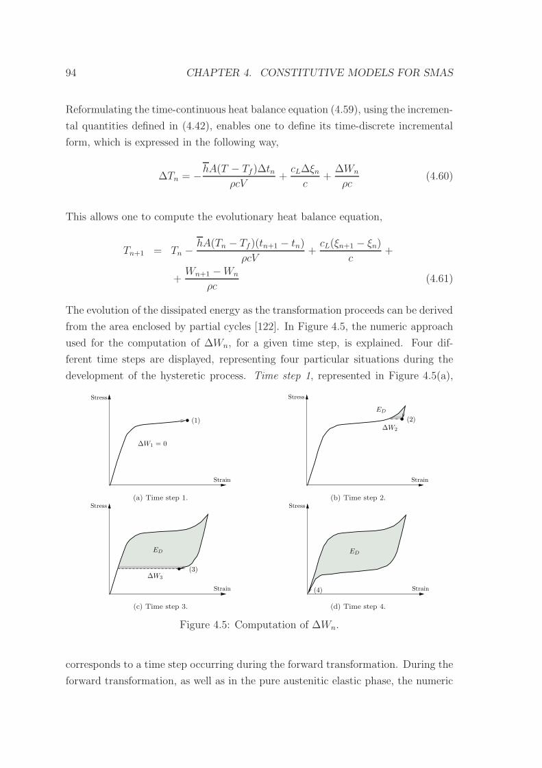
94 CHAPTER 4. CONSTITUTIVE MODELS FOR SMAS
Reformulating the time-continuous heat balance equation (4.59), using the incremen-
tal quantities defined in (4.42), enables one to define its time-discrete incremental
form, which is expressed in the following way,
∆Tn = −hA(T − Tf)∆tn
ρcV+cL∆ξnc
+∆Wn
ρc(4.60)
This allows one to compute the evolutionary heat balance equation,
Tn+1 = Tn −hA(Tn − Tf )(tn+1 − tn)
ρcV+cL(ξn+1 − ξn)
c+
+Wn+1 −Wn
ρc(4.61)
The evolution of the dissipated energy as the transformation proceeds can be derived
from the area enclosed by partial cycles [122]. In Figure 4.5, the numeric approach
used for the computation of ∆Wn, for a given time step, is explained. Four dif-
ferent time steps are displayed, representing four particular situations during the
development of the hysteretic process. Time step 1, represented in Figure 4.5(a),
Strain
Stress
(1)
∆W1 = 0
(a) Time step 1.
Strain
Stress
ED
∆W2
(2)
(b) Time step 2.Stress
Strain
(3)∆W3
ED
(c) Time step 3.
Stress
Strain
ED
(4)
(d) Time step 4.
Figure 4.5: Computation of ∆Wn.
corresponds to a time step occurring during the forward transformation. During the
forward transformation, as well as in the pure austenitic elastic phase, the numeric
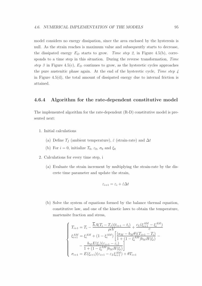
4.6. NUMERICAL IMPLEMENTATION OF THE MODELS 95
model considers no energy dissipation, since the area enclosed by the hysteresis is
null. As the strain reaches is maximum value and subsequently starts to decrease,
the dissipated energy ED starts to grow. Time step 2, in Figure 4.5(b), corre-
sponds to a time step in this situation. During the reverse transformation, Time
step 3 in Figure 4.5(c), ED continues to grow, as the hysteretic cycles approaches
the pure austenitic phase again. At the end of the hysteretic cycle, Time step 4
in Figure 4.5(d), the total amount of dissipated energy due to internal friction is
attained.
4.6.4 Algorithm for the rate-dependent constitutive model
The implemented algorithm for the rate-dependent (R-D) constitutive model is pre-
sented next:
1. Initial calculations
(a) Define Tf (ambient temperature), ε (strain-rate) and ∆t
(b) For i = 0, initialize T0, ε0, σ0 and ξ0
2. Calculations for every time step, i
(a) Evaluate the strain increment by multiplying the strain-rate by the dis-
crete time parameter and update the strain,
εi+1 = εi + ε∆t
(b) Solve the system of equations formed by the balance thermal equation,
constitutive law, and one of the kinetic laws to obtain the temperature,
martensite fraction and stress,
Ti+1 = Ti −hA(Ti − Tf)(ti+1 − ti)
ρcV+cL(ξ
AMi+1 − ξAM
i )c
ξAMi+1 = ξAM
i + (1− ξAMi )
[
(aM − bMθ)(Ti+1 − Ti)1 + (1− ξAM
i )bMH(ξi)−
−bME(ξi)(εi+1 − εi)
1 + (1− ξAMi )bMH(ξi)
]
σi+1 = E(ξi+1)(εi+1 − εLξAMi+1 ) + θTi+1
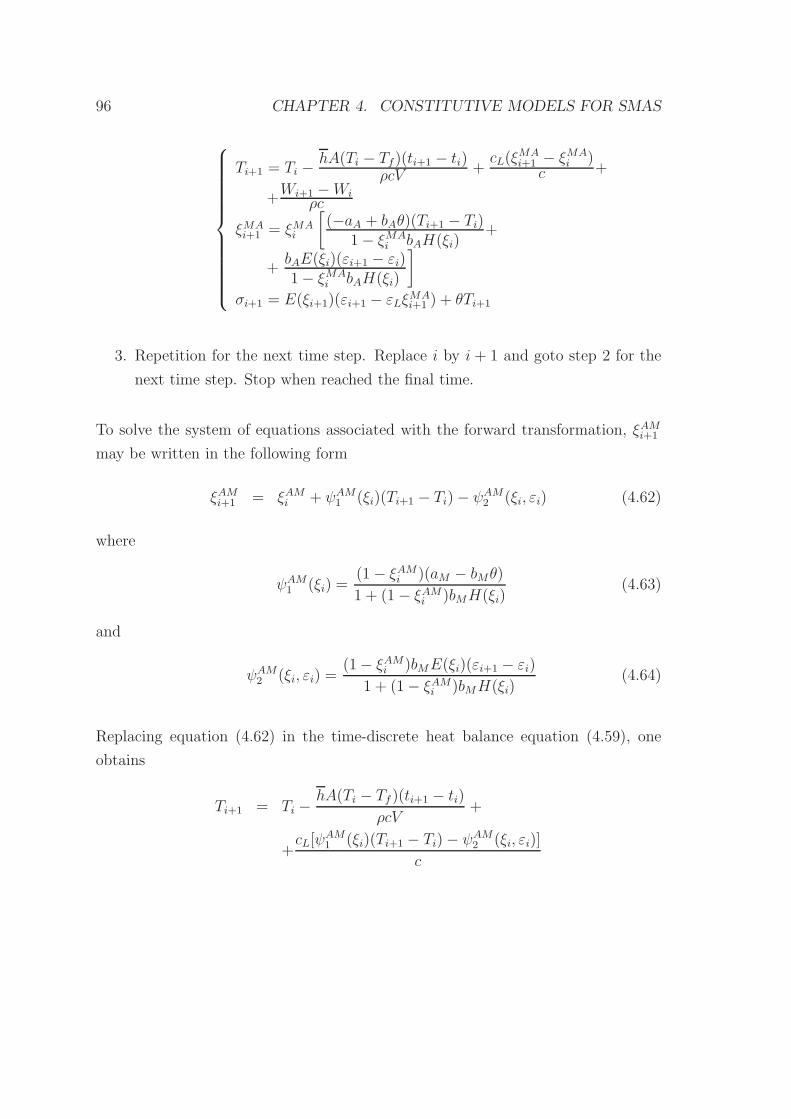
96 CHAPTER 4. CONSTITUTIVE MODELS FOR SMAS
Ti+1 = Ti −hA(Ti − Tf)(ti+1 − ti)
ρcV +cL(ξ
MAi+1 − ξMA
i )c +
+Wi+1 −Wi
ρc
ξMAi+1 = ξMA
i
[
(−aA + bAθ)(Ti+1 − Ti)1− ξMA
i bAH(ξi)+
+bAE(ξi)(εi+1 − εi)1− ξMA
i bAH(ξi)
]
σi+1 = E(ξi+1)(εi+1 − εLξMAi+1 ) + θTi+1
3. Repetition for the next time step. Replace i by i + 1 and goto step 2 for the
next time step. Stop when reached the final time.
To solve the system of equations associated with the forward transformation, ξAMi+1
may be written in the following form
ξAMi+1 = ξAM
i + ψAM1 (ξi)(Ti+1 − Ti)− ψAM
2 (ξi, εi) (4.62)
where
ψAM1 (ξi) =
(1− ξAMi )(aM − bMθ)
1 + (1− ξAMi )bMH(ξi)
(4.63)
and
ψAM2 (ξi, εi) =
(1− ξAMi )bME(ξi)(εi+1 − εi)
1 + (1− ξAMi )bMH(ξi)
(4.64)
Replacing equation (4.62) in the time-discrete heat balance equation (4.59), one
obtains
Ti+1 = Ti −hA(Ti − Tf )(ti+1 − ti)
ρcV+
+cL[ψ
AM1 (ξi)(Ti+1 − Ti)− ψAM
2 (ξi, εi)]
c
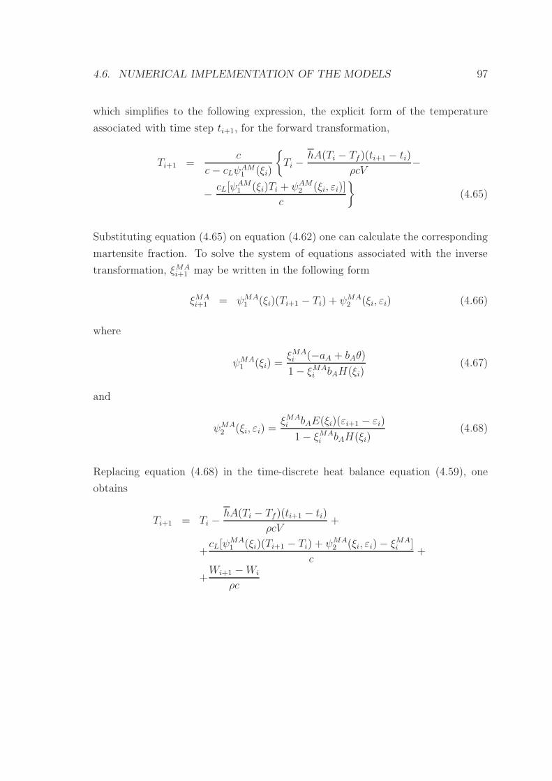
4.6. NUMERICAL IMPLEMENTATION OF THE MODELS 97
which simplifies to the following expression, the explicit form of the temperature
associated with time step ti+1, for the forward transformation,
Ti+1 =c
c− cLψAM1 (ξi)
Ti −hA(Ti − Tf )(ti+1 − ti)
ρcV−
−cL[ψ
AM1 (ξi)Ti + ψAM
2 (ξi, εi)]
c
(4.65)
Substituting equation (4.65) on equation (4.62) one can calculate the corresponding
martensite fraction. To solve the system of equations associated with the inverse
transformation, ξMAi+1 may be written in the following form
ξMAi+1 = ψMA
1 (ξi)(Ti+1 − Ti) + ψMA2 (ξi, εi) (4.66)
where
ψMA1 (ξi) =
ξMAi (−aA + bAθ)
1− ξMAi bAH(ξi)
(4.67)
and
ψMA2 (ξi, εi) =
ξMAi bAE(ξi)(εi+1 − εi)
1− ξMAi bAH(ξi)
(4.68)
Replacing equation (4.68) in the time-discrete heat balance equation (4.59), one
obtains
Ti+1 = Ti −hA(Ti − Tf)(ti+1 − ti)
ρcV+
+cL[ψ
MA1 (ξi)(Ti+1 − Ti) + ψMA
2 (ξi, εi)− ξMAi ]
c+
+Wi+1 −Wi
ρc
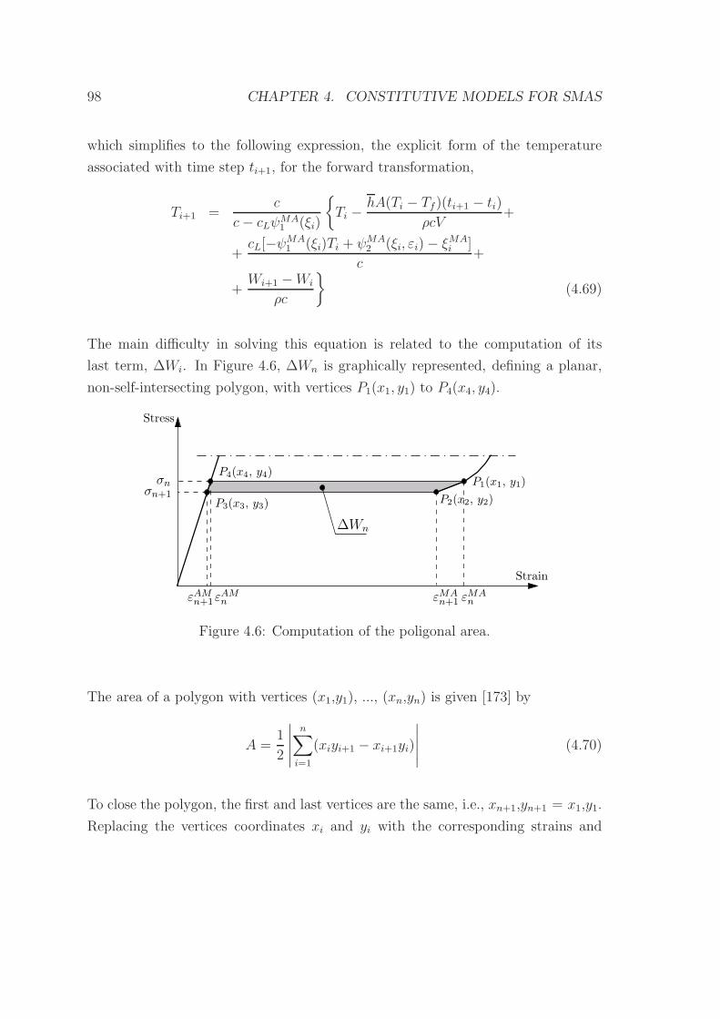
98 CHAPTER 4. CONSTITUTIVE MODELS FOR SMAS
which simplifies to the following expression, the explicit form of the temperature
associated with time step ti+1, for the forward transformation,
Ti+1 =c
c− cLψMA1 (ξi)
Ti −hA(Ti − Tf)(ti+1 − ti)
ρcV+
+cL[−ψ
MA1 (ξi)Ti + ψMA
2 (ξi, εi)− ξMAi ]
c+
+Wi+1 −Wi
ρc
(4.69)
The main difficulty in solving this equation is related to the computation of its
last term, ∆Wi. In Figure 4.6, ∆Wn is graphically represented, defining a planar,
non-self-intersecting polygon, with vertices P1(x1, y1) to P4(x4, y4).
Strain
Stress
P2(x2, y2)σn+1
P3(x3, y3)
P1(x1, y1)P4(x4, y4)
∆Wn
σn
εMAnεMA
n+1εAMnεAM
n+1
Figure 4.6: Computation of the poligonal area.
The area of a polygon with vertices (x1,y1), ..., (xn,yn) is given [173] by
A =1
2
∣
∣
∣
∣
∣
n∑
i=1
(xiyi+1 − xi+1yi)
∣
∣
∣
∣
∣
(4.70)
To close the polygon, the first and last vertices are the same, i.e., xn+1,yn+1 = x1,y1.
Replacing the vertices coordinates xi and yi with the corresponding strains and
4.7. NUMERICAL ASSESSMENT OF THE MODELS 99
stresses represented in Figure 4.6, it yields,
∆Wn =1
2(εMA
n σn+1 − εMAn+1σn + εMA
n+1σn+1 − εAMn+1σn+1 +
+εAMn+1σn − εAM
n σn+1 + εAMn σn − εMA
n σn)
which simplifies to
∆Wn =1
2(εMA
n+1 + εMAn − εAM
n+1 − εAMn )(σn+1 − σn) (4.71)
where εAMn (σn) and ε
AMn+1(σn+1) represent the strains corresponding to σn and σn+1
during the forward transformation. This means that ∆Wi may be computed by
Wi+1 −Wi
ρc=
1
2 ρc(εMA
i+1 + εMAi − εAM
i+1 − εAMi )(σi+1 − σi) (4.72)
Since it is difficult to write the strain value εAMi+1 (σi+1) as an algebraic expression, it
is assumed that ∆Wi ≈ ∆Wi−1 and hence, equation (4.72) may be approximated by
Wi+1 −Wi
ρc≈
1
2 ρc(εMA
i + εMAi−1 − εAM
i − εAMi−1 )(σi − σi−1) (4.73)
In order to solve equation (4.73), a simple iterative searching algorithm is imple-
mented, to extract the values εAMi and εAM
i−1 from the strain vector, knowing σi and
σi−1. Substituting equation (4.73) in equation (4.69), and finally in equation (4.66)
one can calculate the corresponding martensite fraction at step i+1.
4.7 Numerical assessment of the models
The objective of this section is the calibration of the implemented numerical models
and the assessment of their performance in the simulation of the SE stress-strain
response of SMA wires.
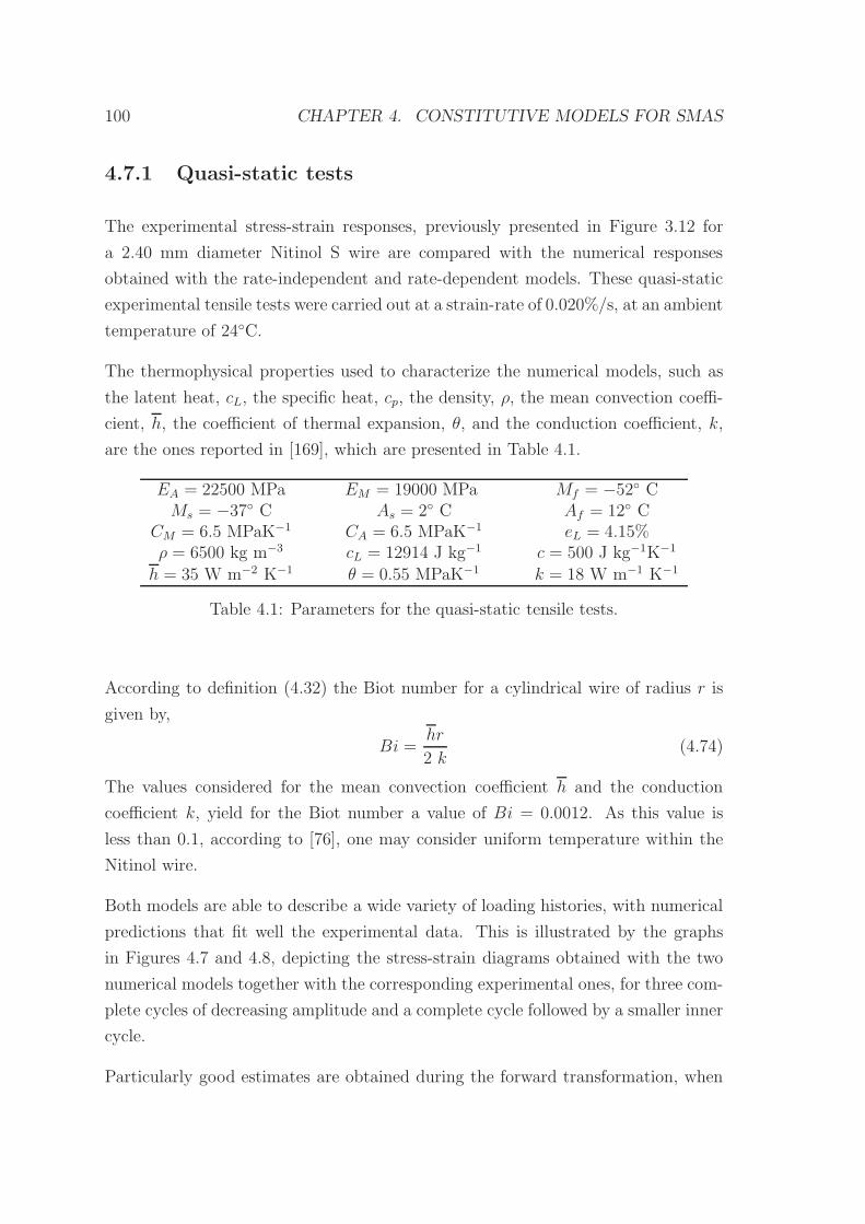
100 CHAPTER 4. CONSTITUTIVE MODELS FOR SMAS
4.7.1 Quasi-static tests
The experimental stress-strain responses, previously presented in Figure 3.12 for
a 2.40 mm diameter Nitinol S wire are compared with the numerical responses
obtained with the rate-independent and rate-dependent models. These quasi-static
experimental tensile tests were carried out at a strain-rate of 0.020%/s, at an ambient
temperature of 24C.
The thermophysical properties used to characterize the numerical models, such as
the latent heat, cL, the specific heat, cp, the density, ρ, the mean convection coeffi-
cient, h, the coefficient of thermal expansion, θ, and the conduction coefficient, k,
are the ones reported in [169], which are presented in Table 4.1.
EA = 22500 MPa EM = 19000 MPa Mf = −52 CMs = −37 C As = 2 C Af = 12 C
CM = 6.5 MPaK−1 CA = 6.5 MPaK−1 eL = 4.15%ρ = 6500 kg m−3 cL = 12914 J kg−1 c = 500 J kg−1K−1
h = 35 W m−2 K−1 θ = 0.55 MPaK−1 k = 18 W m−1 K−1
Table 4.1: Parameters for the quasi-static tensile tests.
According to definition (4.32) the Biot number for a cylindrical wire of radius r is
given by,
Bi =hr
2 k(4.74)
The values considered for the mean convection coefficient h and the conduction
coefficient k, yield for the Biot number a value of Bi = 0.0012. As this value is
less than 0.1, according to [76], one may consider uniform temperature within the
Nitinol wire.
Both models are able to describe a wide variety of loading histories, with numerical
predictions that fit well the experimental data. This is illustrated by the graphs
in Figures 4.7 and 4.8, depicting the stress-strain diagrams obtained with the two
numerical models together with the corresponding experimental ones, for three com-
plete cycles of decreasing amplitude and a complete cycle followed by a smaller inner
cycle.
Particularly good estimates are obtained during the forward transformation, when
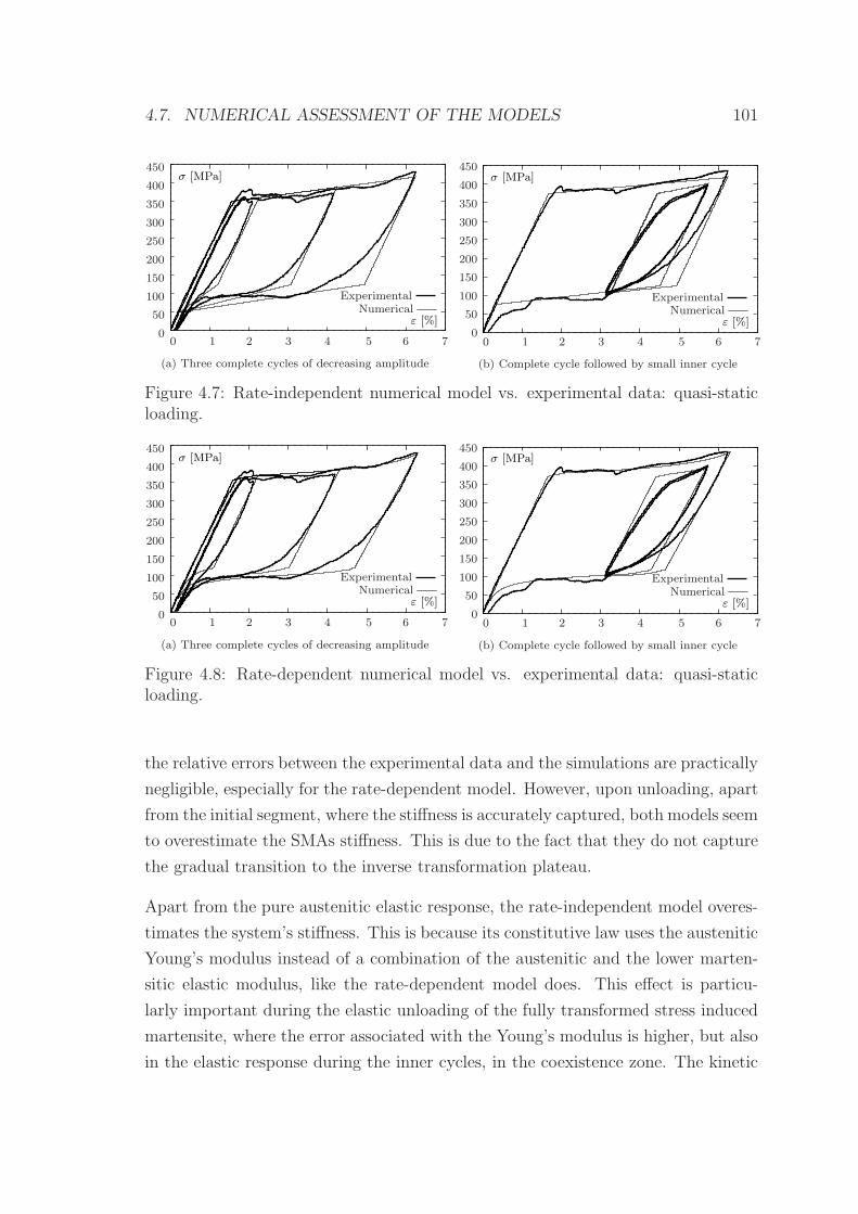
4.7. NUMERICAL ASSESSMENT OF THE MODELS 101
ε [%]
σ [MPa]
70 1 2 3 4 5 60
50
100
150
200
250
300
350
400
450
ExperimentalNumerical
(a) Three complete cycles of decreasing amplitude
ε [%]
σ [MPa]
ExperimentalNumerical
0
50
100
150
200
250
300
350
400
450
70 1 2 3 4 5 6
(b) Complete cycle followed by small inner cycle
Figure 4.7: Rate-independent numerical model vs. experimental data: quasi-staticloading.
σ [MPa]
ε [%]
70 1 2 3 4 5 60
50
100
150
200
250
300
350
400
450
ExperimentalNumerical
(a) Three complete cycles of decreasing amplitude
ε [%]
σ [MPa]
ExperimentalNumerical
0
50
100
150
200
250
300
350
400
450
70 1 2 3 4 5 6
(b) Complete cycle followed by small inner cycle
Figure 4.8: Rate-dependent numerical model vs. experimental data: quasi-staticloading.
the relative errors between the experimental data and the simulations are practically
negligible, especially for the rate-dependent model. However, upon unloading, apart
from the initial segment, where the stiffness is accurately captured, both models seem
to overestimate the SMAs stiffness. This is due to the fact that they do not capture
the gradual transition to the inverse transformation plateau.
Apart from the pure austenitic elastic response, the rate-independent model overes-
timates the system’s stiffness. This is because its constitutive law uses the austenitic
Young’s modulus instead of a combination of the austenitic and the lower marten-
sitic elastic modulus, like the rate-dependent model does. This effect is particu-
larly important during the elastic unloading of the fully transformed stress induced
martensite, where the error associated with the Young’s modulus is higher, but also
in the elastic response during the inner cycles, in the coexistence zone. The kinetic
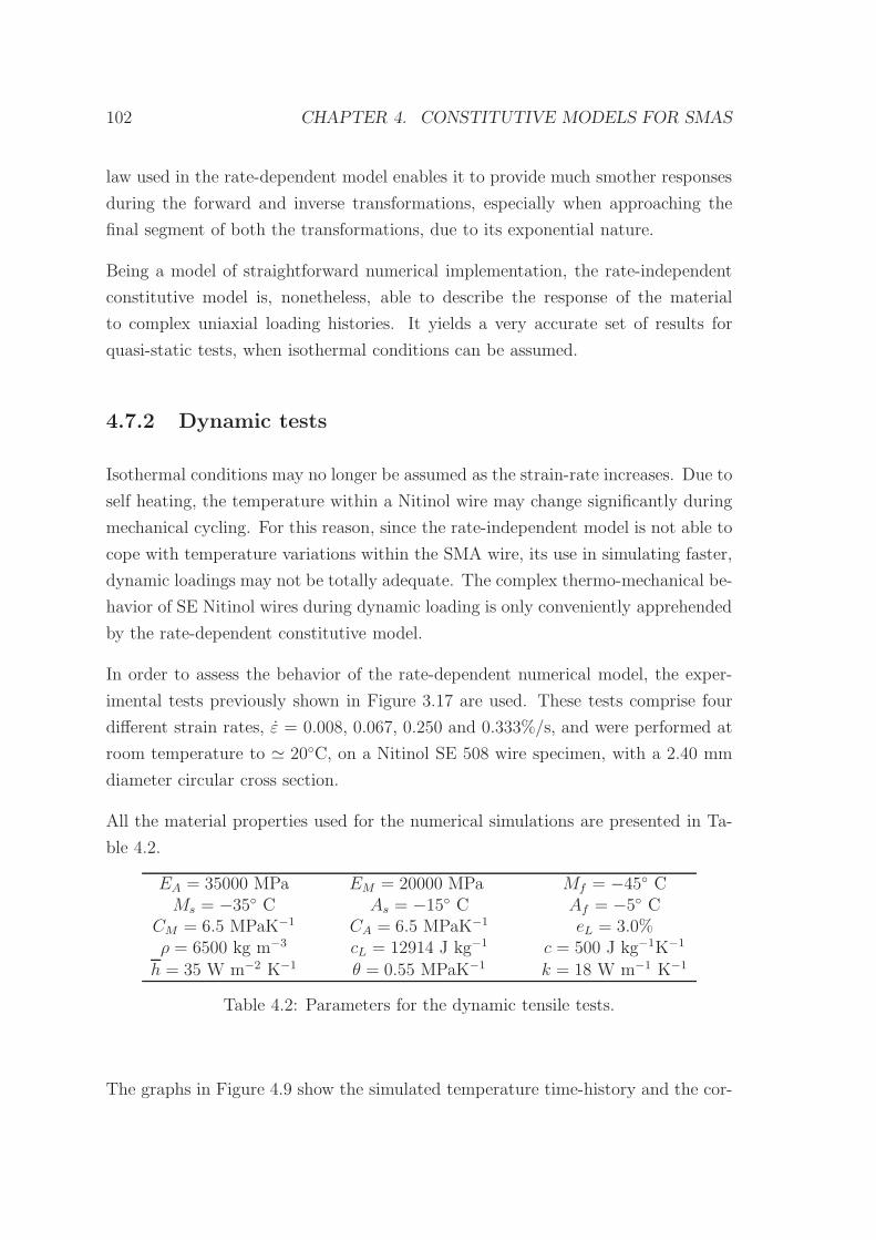
102 CHAPTER 4. CONSTITUTIVE MODELS FOR SMAS
law used in the rate-dependent model enables it to provide much smother responses
during the forward and inverse transformations, especially when approaching the
final segment of both the transformations, due to its exponential nature.
Being a model of straightforward numerical implementation, the rate-independent
constitutive model is, nonetheless, able to describe the response of the material
to complex uniaxial loading histories. It yields a very accurate set of results for
quasi-static tests, when isothermal conditions can be assumed.
4.7.2 Dynamic tests
Isothermal conditions may no longer be assumed as the strain-rate increases. Due to
self heating, the temperature within a Nitinol wire may change significantly during
mechanical cycling. For this reason, since the rate-independent model is not able to
cope with temperature variations within the SMA wire, its use in simulating faster,
dynamic loadings may not be totally adequate. The complex thermo-mechanical be-
havior of SE Nitinol wires during dynamic loading is only conveniently apprehended
by the rate-dependent constitutive model.
In order to assess the behavior of the rate-dependent numerical model, the exper-
imental tests previously shown in Figure 3.17 are used. These tests comprise four
different strain rates, ε = 0.008, 0.067, 0.250 and 0.333%/s, and were performed at
room temperature to ≃ 20C, on a Nitinol SE 508 wire specimen, with a 2.40 mm
diameter circular cross section.
All the material properties used for the numerical simulations are presented in Ta-
ble 4.2.
EA = 35000 MPa EM = 20000 MPa Mf = −45 CMs = −35 C As = −15 C Af = −5 C
CM = 6.5 MPaK−1 CA = 6.5 MPaK−1 eL = 3.0%ρ = 6500 kg m−3 cL = 12914 J kg−1 c = 500 J kg−1K−1
h = 35 W m−2 K−1 θ = 0.55 MPaK−1 k = 18 W m−1 K−1
Table 4.2: Parameters for the dynamic tensile tests.
The graphs in Figure 4.9 show the simulated temperature time-history and the cor-
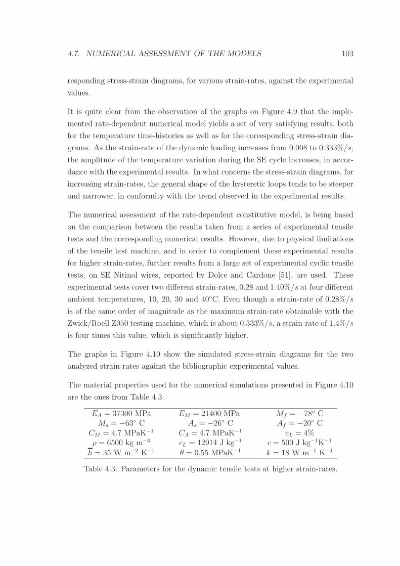
4.7. NUMERICAL ASSESSMENT OF THE MODELS 103
responding stress-strain diagrams, for various strain-rates, against the experimental
values.
It is quite clear from the observation of the graphs on Figure 4.9 that the imple-
mented rate-dependent numerical model yields a set of very satisfying results, both
for the temperature time-histories as well as for the corresponding stress-strain dia-
grams. As the strain-rate of the dynamic loading increases from 0.008 to 0.333%/s,
the amplitude of the temperature variation during the SE cycle increases, in accor-
dance with the experimental results. In what concerns the stress-strain diagrams, for
increasing strain-rates, the general shape of the hysteretic loops tends to be steeper
and narrower, in conformity with the trend observed in the experimental results.
The numerical assessment of the rate-dependent constitutive model, is being based
on the comparison between the results taken from a series of experimental tensile
tests and the corresponding numerical results. However, due to physical limitations
of the tensile test machine, and in order to complement these experimental results
for higher strain-rates, further results from a large set of experimental cyclic tensile
tests, on SE Nitinol wires, reported by Dolce and Cardone [51], are used. These
experimental tests cover two different strain-rates, 0.28 and 1.40%/s at four different
ambient temperatures, 10, 20, 30 and 40C. Even though a strain-rate of 0.28%/s
is of the same order of magnitude as the maximum strain-rate obtainable with the
Zwick/Roell Z050 testing machine, which is about 0.333%/s, a strain-rate of 1.4%/s
is four times this value, which is significantly higher.
The graphs in Figure 4.10 show the simulated stress-strain diagrams for the two
analyzed strain-rates against the bibliographic experimental values.
The material properties used for the numerical simulations presented in Figure 4.10
are the ones from Table 4.3.
EA = 37300 MPa EM = 21400 MPa Mf = −78 CMs = −63 C As = −26 C Af = −20 C
CM = 4.7 MPaK−1 CA = 4.7 MPaK−1 eL = 4%ρ = 6500 kg m−3 cL = 12914 J kg−1 c = 500 J kg−1K−1
h = 35 W m−2 K−1 θ = 0.55 MPaK−1 k = 18 W m−1 K−1
Table 4.3: Parameters for the dynamic tensile tests at higher strain-rates.
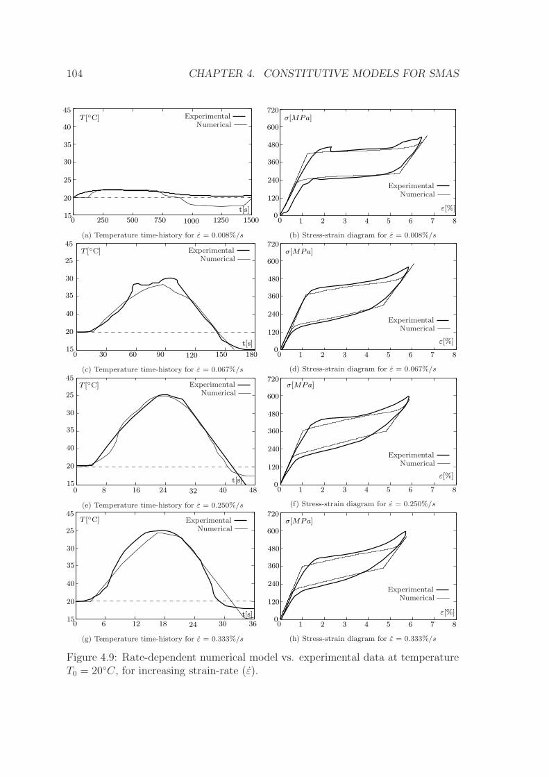
104 CHAPTER 4. CONSTITUTIVE MODELS FOR SMAS
0 250 500 750 1000 1250 1500
20
25
30
35
40
15
45
t[s]
T [C] ExperimentalNumerical
(a) Temperature time-history for ε = 0.008%/s
1 2 4 5 6 7 830
240
360
480
600
120
0
720σ[MPa]
ε[%]
ExperimentalNumerical
(b) Stress-strain diagram for ε = 0.008%/s
0 30 60 90 120 150 180
40
35
30
25
20
45
15t[s]
T [C] ExperimentalNumerical
(c) Temperature time-history for ε = 0.067%/s
1 2 4 5 6 7 83
720
240
360
480
600
120
00
σ[MPa]
ε[%]
ExperimentalNumerical
(d) Stress-strain diagram for ε = 0.067%/s
32 40 480 16 248
40
35
30
25
20
45
15 t[s]
T [C] ExperimentalNumerical
(e) Temperature time-history for ε = 0.250%/s
1 2 4 5 6 7 83
720
240
360
480
600
120
00
σ[MPa]
ε[%]
ExperimentalNumerical
(f) Stress-strain diagram for ε = 0.250%/s
40
35
30
20
45
150 36302418126
25
t[s]
T [C] ExperimentalNumerical
(g) Temperature time-history for ε = 0.333%/s
1 2 4 5 6 7 83
720
240
360
480
600
120
00
σ[MPa]
ε[%]
ExperimentalNumerical
(h) Stress-strain diagram for ε = 0.333%/s
Figure 4.9: Rate-dependent numerical model vs. experimental data at temperatureT0 = 20C, for increasing strain-rate (ε).
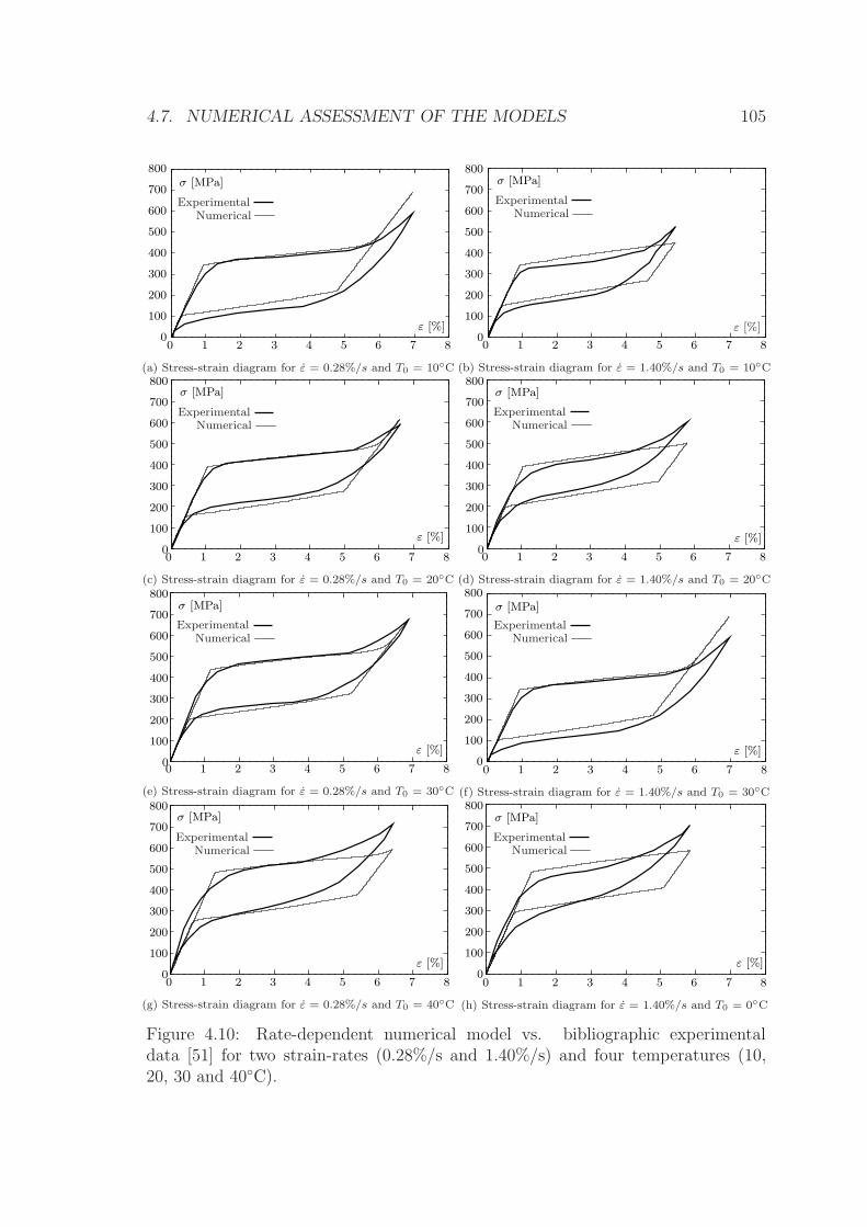
4.7. NUMERICAL ASSESSMENT OF THE MODELS 105
0 1 2 3 4 5 6 7 8
σ [MPa]800
700
600
500
300
200
100
0ε [%]
400
ExperimentalNumerical
(a) Stress-strain diagram for ε = 0.28%/s and T0 = 10C
800
700
600
500
300
200
100
0
400
0 1 2 3 4 5 6 7 8
σ [MPa]
ExperimentalNumerical
ε [%]
(b) Stress-strain diagram for ε = 1.40%/s and T0 = 10C800
700
600
500
300
200
100
0
400
0 1 2 3 4 5 6 7 8
σ [MPa]
ε [%]
ExperimentalNumerical
(c) Stress-strain diagram for ε = 0.28%/s and T0 = 20C
0 1 2 3 4 5 6 7 8
800
700
600
500
300
200
100
0
400
σ [MPa]
ε [%]
ExperimentalNumerical
(d) Stress-strain diagram for ε = 1.40%/s and T0 = 20C800
700
600
500
300
200
100
0
400
0 1 2 3 4 5 6 7 8
σ [MPa]
ε [%]
ExperimentalNumerical
(e) Stress-strain diagram for ε = 0.28%/s and T0 = 30C
0 1 2 3 4 5 6 7 8
σ [MPa]800
700
600
500
300
200
100
0ε [%]
400
ExperimentalNumerical
(f) Stress-strain diagram for ε = 1.40%/s and T0 = 30C
0 1 2 3 4 5 6 7 8
800
700
600
500
300
200
100
0
400
σ [MPa]
ε [%]
ExperimentalNumerical
(g) Stress-strain diagram for ε = 0.28%/s and T0 = 40C
0
800
700
600
500
300
200
100
400
0 1 2 3 4 5 6 7 8
σ [MPa]
ε [%]
ExperimentalNumerical
(h) Stress-strain diagram for ε = 1.40%/s and T0 = 0C
Figure 4.10: Rate-dependent numerical model vs. bibliographic experimentaldata [51] for two strain-rates (0.28%/s and 1.40%/s) and four temperatures (10,20, 30 and 40C).
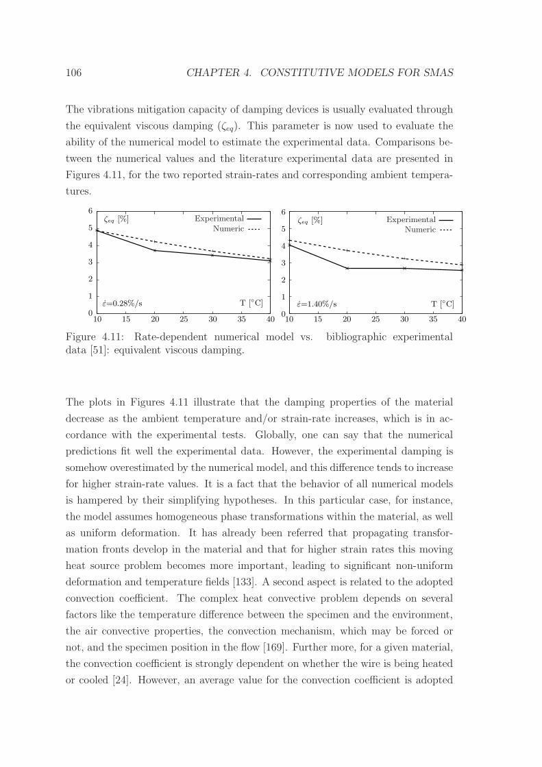
106 CHAPTER 4. CONSTITUTIVE MODELS FOR SMAS
The vibrations mitigation capacity of damping devices is usually evaluated through
the equivalent viscous damping (ζeq). This parameter is now used to evaluate the
ability of the numerical model to estimate the experimental data. Comparisons be-
tween the numerical values and the literature experimental data are presented in
Figures 4.11, for the two reported strain-rates and corresponding ambient tempera-
tures.
10 15 20 25 30 35 400
1
2
3
4
5ζeq [%]
6
ε=0.28%/s T [C]
ExperimentalNumeric
0
1
2
3
4
5
6
10 15 20 25 30 35 40
ζeq [%]
ε=1.40%/s T [C]
ExperimentalNumeric
Figure 4.11: Rate-dependent numerical model vs. bibliographic experimentaldata [51]: equivalent viscous damping.
The plots in Figures 4.11 illustrate that the damping properties of the material
decrease as the ambient temperature and/or strain-rate increases, which is in ac-
cordance with the experimental tests. Globally, one can say that the numerical
predictions fit well the experimental data. However, the experimental damping is
somehow overestimated by the numerical model, and this difference tends to increase
for higher strain-rate values. It is a fact that the behavior of all numerical models
is hampered by their simplifying hypotheses. In this particular case, for instance,
the model assumes homogeneous phase transformations within the material, as well
as uniform deformation. It has already been referred that propagating transfor-
mation fronts develop in the material and that for higher strain rates this moving
heat source problem becomes more important, leading to significant non-uniform
deformation and temperature fields [133]. A second aspect is related to the adopted
convection coefficient. The complex heat convective problem depends on several
factors like the temperature difference between the specimen and the environment,
the air convective properties, the convection mechanism, which may be forced or
not, and the specimen position in the flow [169]. Further more, for a given material,
the convection coefficient is strongly dependent on whether the wire is being heated
or cooled [24]. However, an average value for the convection coefficient is adopted
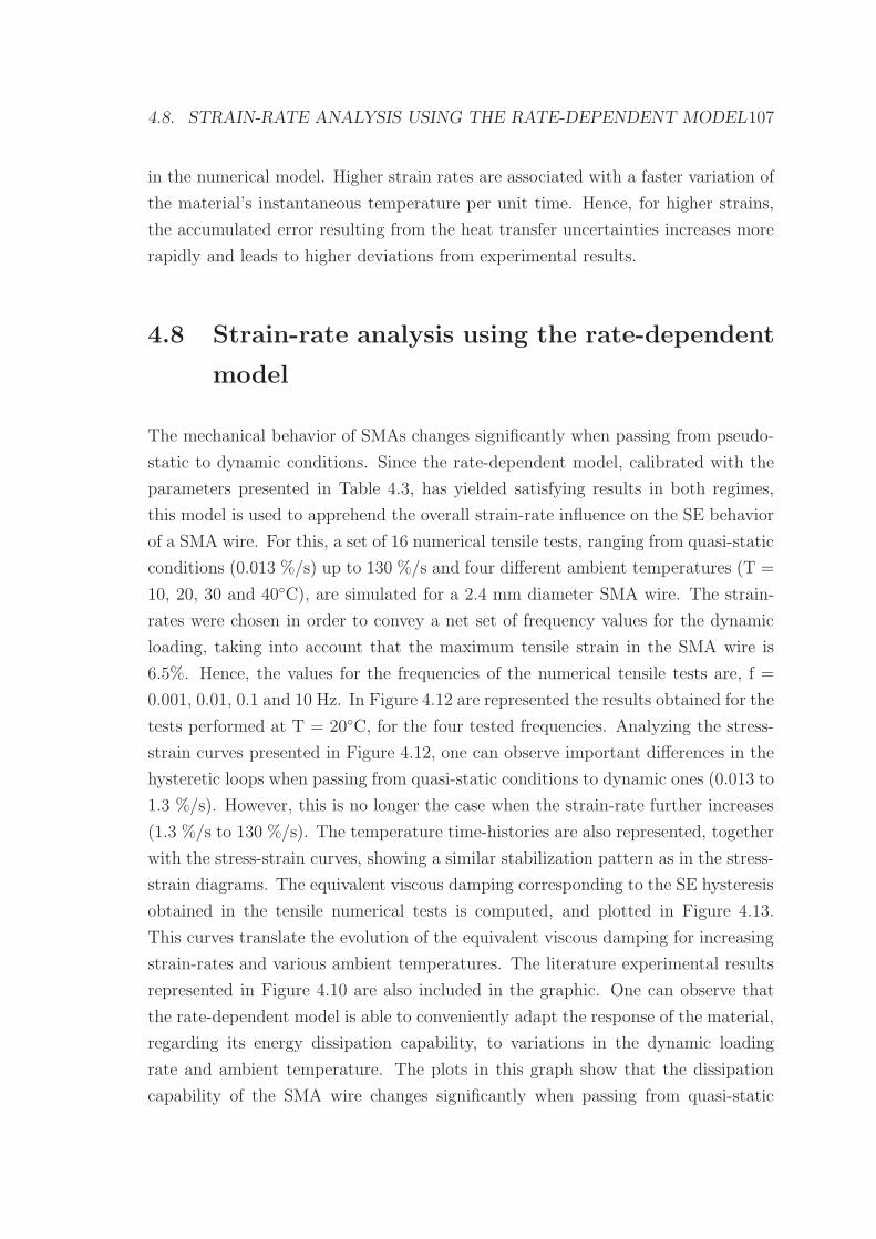
4.8. STRAIN-RATE ANALYSIS USING THE RATE-DEPENDENT MODEL107
in the numerical model. Higher strain rates are associated with a faster variation of
the material’s instantaneous temperature per unit time. Hence, for higher strains,
the accumulated error resulting from the heat transfer uncertainties increases more
rapidly and leads to higher deviations from experimental results.
4.8 Strain-rate analysis using the rate-dependent
model
The mechanical behavior of SMAs changes significantly when passing from pseudo-
static to dynamic conditions. Since the rate-dependent model, calibrated with the
parameters presented in Table 4.3, has yielded satisfying results in both regimes,
this model is used to apprehend the overall strain-rate influence on the SE behavior
of a SMA wire. For this, a set of 16 numerical tensile tests, ranging from quasi-static
conditions (0.013 %/s) up to 130 %/s and four different ambient temperatures (T =
10, 20, 30 and 40C), are simulated for a 2.4 mm diameter SMA wire. The strain-
rates were chosen in order to convey a net set of frequency values for the dynamic
loading, taking into account that the maximum tensile strain in the SMA wire is
6.5%. Hence, the values for the frequencies of the numerical tensile tests are, f =
0.001, 0.01, 0.1 and 10 Hz. In Figure 4.12 are represented the results obtained for the
tests performed at T = 20C, for the four tested frequencies. Analyzing the stress-
strain curves presented in Figure 4.12, one can observe important differences in the
hysteretic loops when passing from quasi-static conditions to dynamic ones (0.013 to
1.3 %/s). However, this is no longer the case when the strain-rate further increases
(1.3 %/s to 130 %/s). The temperature time-histories are also represented, together
with the stress-strain curves, showing a similar stabilization pattern as in the stress-
strain diagrams. The equivalent viscous damping corresponding to the SE hysteresis
obtained in the tensile numerical tests is computed, and plotted in Figure 4.13.
This curves translate the evolution of the equivalent viscous damping for increasing
strain-rates and various ambient temperatures. The literature experimental results
represented in Figure 4.10 are also included in the graphic. One can observe that
the rate-dependent model is able to conveniently adapt the response of the material,
regarding its energy dissipation capability, to variations in the dynamic loading
rate and ambient temperature. The plots in this graph show that the dissipation
capability of the SMA wire changes significantly when passing from quasi-static
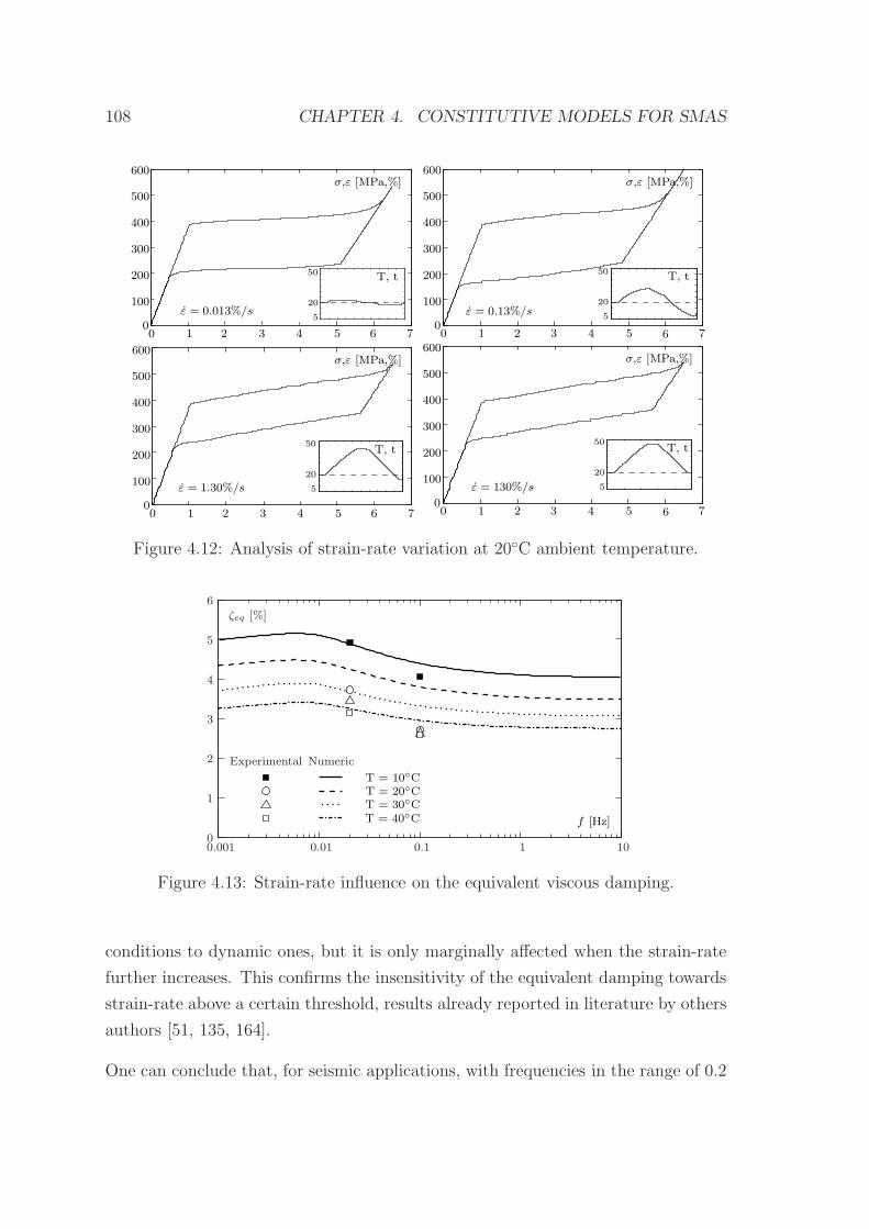
108 CHAPTER 4. CONSTITUTIVE MODELS FOR SMAS
50
20
5
50
20
5
50
20
5
50
20
5
600
500
400
300
200
100
600
500
400
300
200
100
600
500
400
300
200
100
600
500
400
300
200
100
00 5431 7
00 5431 7
00 5431 7
6
600 5431 76
62
2
2
2
ε = 0.013%/s ε = 0.13%/s
ε = 1.30%/s ε = 130%/s
σ,ε [MPa,%]σ,ε [MPa,%]
σ,ε [MPa,%] σ,ε [MPa,%]
T, t T, t
T, t T, t
Figure 4.12: Analysis of strain-rate variation at 20C ambient temperature.
f [Hz]
T = 30C
T = 10CT = 20C
T = 40C
NumericExperimental
0
1
2
3
4
5
6
0.001 0.01 0.1 1 10
ζeq [%]
Figure 4.13: Strain-rate influence on the equivalent viscous damping.
conditions to dynamic ones, but it is only marginally affected when the strain-rate
further increases. This confirms the insensitivity of the equivalent damping towards
strain-rate above a certain threshold, results already reported in literature by others
authors [51, 135, 164].
One can conclude that, for seismic applications, with frequencies in the range of 0.2
4.9. CLOSURE 109
to 4 Hz, the behavior of SMA wires is mainly insensitive to strain-rate. Accordingly,
for this type of applications, SMA models that are insensitive to strain-rate can still
be adequate for simulating the response of structures including SMA elements, once
calibrated with dynamic experimental tests [6].
4.9 Closure
Two constitutive models for the mathematical modeling of SMAs are described.
Both rate-independent and a rate-dependent constitutive models are analyzed, re-
garding their mechanical and kinetic laws. The heat transfer problem due to the
thermodynamics underlying the transformation processes is also addressed, for the
rate-dependent constitutive model.
Several mechanical laws are addressed, relating stress (σ), strain (ε), temperature
(T ) and martensite fraction (ξ), which can be regarded as the fraction of the pro-
duced phase. This transformed phase fraction is considered to be in series with the
elastic fraction of the response. Three approaches for the mathematical modeling of
this elastic component are presented, namely the Voight scheme, the Reuss scheme
and the simple linear model.
Regarding the transformation kinetic laws, describing the evolution of the marten-
site fraction with stress and temperature based in the material’s stress-temperature
phase diagram, linear and exponential laws are analyzed.
The heat transfer problem is also studied, and a practical approach to the analysis
of the convective heat transfer from surfaces is presented.
Having discussed the theoretical background concerning constitutive models for
SMAs, a rate-independent model and a rate-dependent model are implemented.
These numerical implementations consist of strain-driven, time-discrete models,
making use of the Euler method to enable the transformation of the time-continuous
evolutionary equations into time-discrete evolutionary equations. The algorithms for
both constitutive models, which are presented in detail, are implemented in a Matlab
R2007a environment.
The performance of the implemented numerical models in quasi-static and dynamic

110 CHAPTER 4. CONSTITUTIVE MODELS FOR SMAS
simulations of the SE stress-strain and temperature responses of SMA wires is an-
alyzed. The results yielded by the simulations are successfully compared with ex-
perimental and bibliographic data. A strain-rate analysis is performed using the
rate-dependent model which allowed to conclude that for seismic applications, with
frequencies in the range of 0.2 to 4 Hz, the behavior of SMA wires is mainly insen-
sitive to strain-rate. This shows that rate-independent constitutive models can still
be rather efficient in simulating SMA’s behavior, in this frequency range.
Chapter 5
Modeling of Superelastic
Vibration Control Devices
5.1 Introduction
This chapter focuses on a series of numerical simulations of dynamic systems com-
prising SE components. The main purpose of these simulations is to assess the
potential of SE SMAs in the vibration control of structures, namely in seismic con-
trol devices. A comparison between the rate-independent and the rate-dependent
constitutive models is made.
The calibrated numerical models are used to investigate the dynamic response of sev-
eral vibration control devices built up of austenitic SE wires. Their energy dissipa-
tion and re-centering capabilities, important features of these devices, are addressed
in the numerical tests. The sensitivity of these devices to ambient temperature,
strain-rate and strain-amplitude is also analyzed. One of these devices is tested as a
seismic passive vibration control system in a numerical model of a railway viaduct,
subjected to different ground accelerations.
111
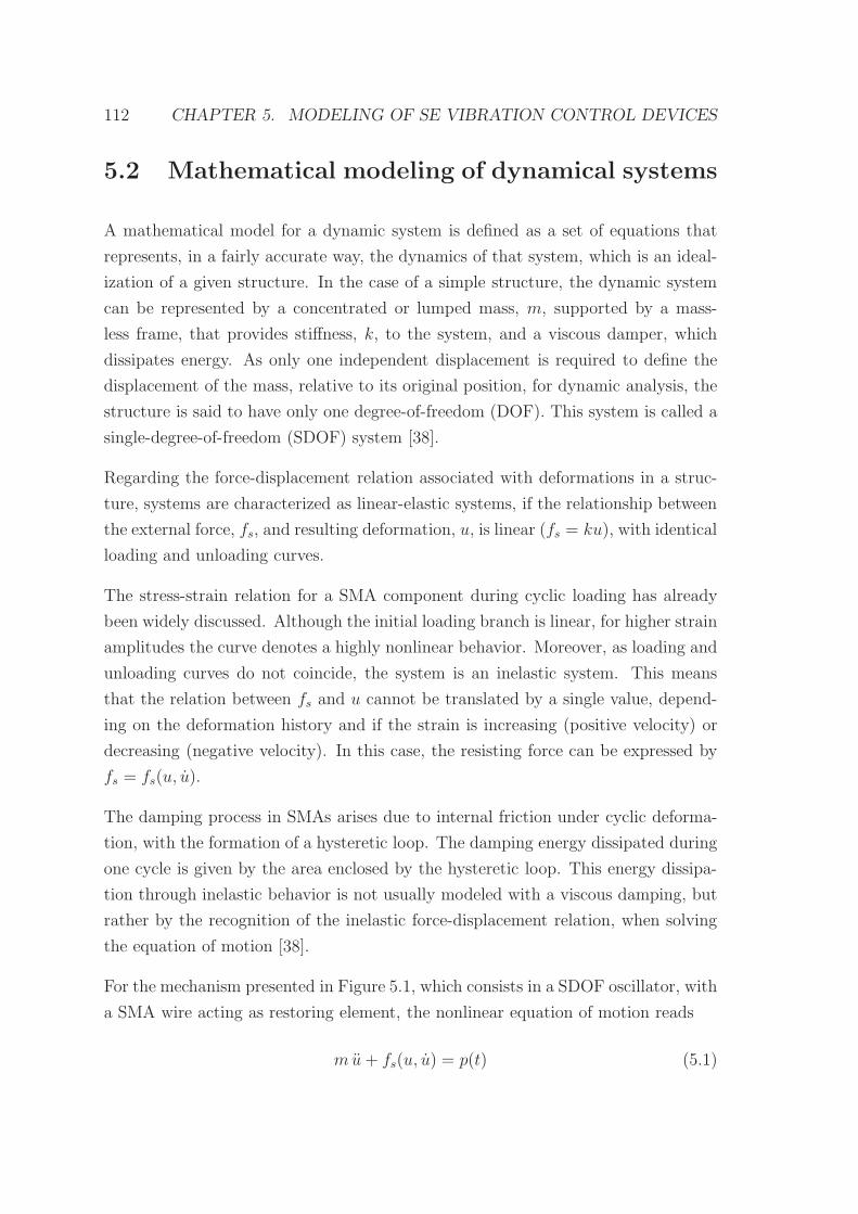
112 CHAPTER 5. MODELING OF SE VIBRATION CONTROL DEVICES
5.2 Mathematical modeling of dynamical systems
A mathematical model for a dynamic system is defined as a set of equations that
represents, in a fairly accurate way, the dynamics of that system, which is an ideal-
ization of a given structure. In the case of a simple structure, the dynamic system
can be represented by a concentrated or lumped mass, m, supported by a mass-
less frame, that provides stiffness, k, to the system, and a viscous damper, which
dissipates energy. As only one independent displacement is required to define the
displacement of the mass, relative to its original position, for dynamic analysis, the
structure is said to have only one degree-of-freedom (DOF). This system is called a
single-degree-of-freedom (SDOF) system [38].
Regarding the force-displacement relation associated with deformations in a struc-
ture, systems are characterized as linear-elastic systems, if the relationship between
the external force, fs, and resulting deformation, u, is linear (fs = ku), with identical
loading and unloading curves.
The stress-strain relation for a SMA component during cyclic loading has already
been widely discussed. Although the initial loading branch is linear, for higher strain
amplitudes the curve denotes a highly nonlinear behavior. Moreover, as loading and
unloading curves do not coincide, the system is an inelastic system. This means
that the relation between fs and u cannot be translated by a single value, depend-
ing on the deformation history and if the strain is increasing (positive velocity) or
decreasing (negative velocity). In this case, the resisting force can be expressed by
fs = fs(u, u).
The damping process in SMAs arises due to internal friction under cyclic deforma-
tion, with the formation of a hysteretic loop. The damping energy dissipated during
one cycle is given by the area enclosed by the hysteretic loop. This energy dissipa-
tion through inelastic behavior is not usually modeled with a viscous damping, but
rather by the recognition of the inelastic force-displacement relation, when solving
the equation of motion [38].
For the mechanism presented in Figure 5.1, which consists in a SDOF oscillator, with
a SMA wire acting as restoring element, the nonlinear equation of motion reads
mu+ fs(u, u) = p(t) (5.1)
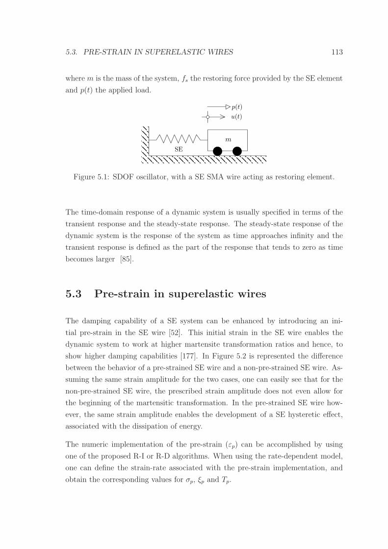
5.3. PRE-STRAIN IN SUPERELASTIC WIRES 113
where m is the mass of the system, fs the restoring force provided by the SE element
and p(t) the applied load.
u(t)
p(t)
m
SE
Figure 5.1: SDOF oscillator, with a SE SMA wire acting as restoring element.
The time-domain response of a dynamic system is usually specified in terms of the
transient response and the steady-state response. The steady-state response of the
dynamic system is the response of the system as time approaches infinity and the
transient response is defined as the part of the response that tends to zero as time
becomes larger [85].
5.3 Pre-strain in superelastic wires
The damping capability of a SE system can be enhanced by introducing an ini-
tial pre-strain in the SE wire [52]. This initial strain in the SE wire enables the
dynamic system to work at higher martensite transformation ratios and hence, to
show higher damping capabilities [177]. In Figure 5.2 is represented the difference
between the behavior of a pre-strained SE wire and a non-pre-strained SE wire. As-
suming the same strain amplitude for the two cases, one can easily see that for the
non-pre-strained SE wire, the prescribed strain amplitude does not even allow for
the beginning of the martensitic transformation. In the pre-strained SE wire how-
ever, the same strain amplitude enables the development of a SE hysteretic effect,
associated with the dissipation of energy.
The numeric implementation of the pre-strain (εp) can be accomplished by using
one of the proposed R-I or R-D algorithms. When using the rate-dependent model,
one can define the strain-rate associated with the pre-strain implementation, and
obtain the corresponding values for σp, ξp and Tp.
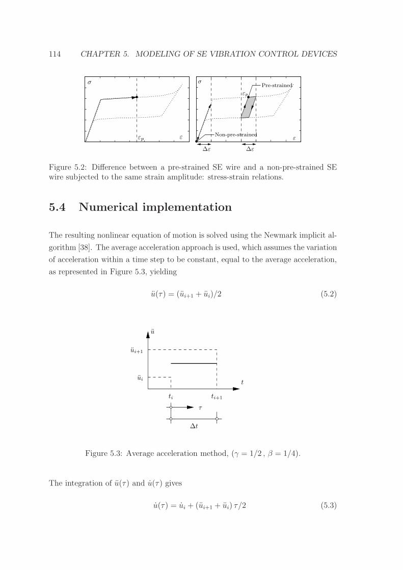
114 CHAPTER 5. MODELING OF SE VIBRATION CONTROL DEVICES
σ
ε
∆ε ∆ε
Pre-strained
Non-pre-strained
εp
σ
εεp
Figure 5.2: Difference between a pre-strained SE wire and a non-pre-strained SEwire subjected to the same strain amplitude: stress-strain relations.
5.4 Numerical implementation
The resulting nonlinear equation of motion is solved using the Newmark implicit al-
gorithm [38]. The average acceleration approach is used, which assumes the variation
of acceleration within a time step to be constant, equal to the average acceleration,
as represented in Figure 5.3, yielding
u(τ) = (ui+1 + ui)/2 (5.2)
τ
∆t
ui
ui+1
ti ti+1
t
u
Figure 5.3: Average acceleration method, (γ = 1/2 , β = 1/4).
The integration of u(τ) and u(τ) gives
u(τ) = ui + (ui+1 + ui) τ/2 (5.3)

5.4. NUMERICAL IMPLEMENTATION 115
and
u(τ) = ui + uiτ + (ui+1 + ui) τ2/4 (5.4)
To evaluate the velocity ui+1 and the displacement ui+1, at time i + 1, one has to
replace τ by ∆ t, in equations (5.3) and (5.4) to yield
ui+1 = ui + (ui+1 + ui)∆t/2 and (5.5)
and
ui+1 = ui + ui∆t + (ui+1 + ui) (∆t)2/4 (5.6)
5.4.1 Algorithm to solve the equation of motion
The implemented algorithm is presented next, for the R-D approach:
1. Initial calculations
(a) Define Tf (ambient temperature), εp (pre-strain), u0 (initial displace-
ment) and ∆t
(b) Introduce pre-strain (εp): compute σp, ξp, Tp, and kp using R-D algorithm
(c) Introduce initial displacement (u0) : compute ε0, σ0, ξ0, T0 and k0 using
R-D algorithm
(d) For i = 0, initialize ε0, σ0, ξ0, T0 and k0
(e) Compute initial acceleration:
u0 =p0 − cu0 − (fs)0
m
(f) Compute Newmark’s constants:
a =1
β∆tm+
γ
βc and b =
1
2βm+∆t
(
γ
2β− 1
)
c
2. Calculations for each time step, i
116 CHAPTER 5. MODELING OF SE VIBRATION CONTROL DEVICES
(a) Compute initial acceleration:
∆pi = ∆pi + aui + bui
(b) Determine the tangent stiffness ki
(c)
ki = ki +γ
β∆tc+
1
β(∆t)2m
(d) Solve for ∆ui from ki and ∆pi using the modified Newton-Raphson iter-
ative procedure
i. Initialize data
u(0)i+1 = ui f (0)
s = (fs)i ∆R(1) = ∆pi kT = ki
ii. Calculation for each iteration ∆u(j) = ∆R(j)/kT u(j)i+1 = u
(j−1)i+1 +∆u(j) Compute f
(j)s using R-D algorithm ∆f (j) = f
(j)s − f
(j−1)s + (kT − kT )∆u
(j) ∆R(j+1) = ∆R(j) −∆f (j)
iii. Repetition for next iteration. Replace j by j +1 and repeat calcula-
tion steps 2(d)ii until ∆u(j) < ε
(e)
∆ui =γ
β∆t∆ui −
γ
βui +∆t
(
1−γ
2β
)
ui
If a change of sign in velocity occurs, compute a new time step and
recompute step 2a
(f)
∆ui =1
β(∆t)2∆ui −
1
β∆tui −
1
2βui
(g)
ui+1 = ui +∆ui and ui+1 = ui +∆ui
3. Repetition for the next time step. Replace i by i + 1 and repeat step 2a for
the next time step. Stop when reached the final time.
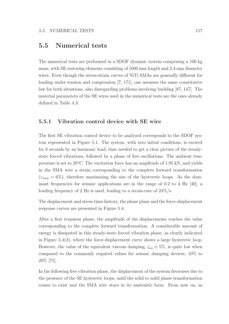
5.5. NUMERICAL TESTS 117
5.5 Numerical tests
The numerical tests are performed in a SDOF dynamic system comprising a 100 kg
mass, with SE restoring elements consisting of 1000 mm length and 2.4 mm diameter
wires. Even though the stress-strain curves of NiTi SMAs are generally different for
loading under tension and compression [?, 171], one assumes the same constitutive
law for both situations, also disregarding problems involving buckling [87, 147]. The
material parameters of the SE wires used in the numerical tests are the ones already
defined in Table 4.3.
5.5.1 Vibration control device with SE wire
The first SE vibration control device to be analyzed corresponds to the SDOF sys-
tem represented in Figure 5.1. The system, with zero initial conditions, is excited
for 8 seconds by an harmonic load, time needed to get a clear picture of the steady-
state forced vibrations, followed by a phase of free oscillations. The ambient tem-
perature is set to 20C. The excitation force has an amplitude of 1.95 kN, and yields
in the SMA wire a strain corresponding to the complete forward transformation
(εmax = 6%), therefore maximizing the size of the hysteretic loops. As the dom-
inant frequencies for seismic applications are in the range of 0.2 to 4 Hz [40], a
loading frequency of 2 Hz is used, leading to a strain-rate of 24%/s.
The displacement and stress time-history, the phase plane and the force-displacement
response curves are presented in Figure 5.4.
After a first transient phase, the amplitude of the displacements reaches the value
corresponding to the complete forward transformation. A considerable amount of
energy is dissipated in this steady-state forced vibration phase, as clearly indicated
in Figure 5.4(d), where the force-displacement curve shows a large hysteretic loop.
However, the value of the equivalent viscous damping, ζeq ≃ 5%, is quite low when
compared to the commonly required values for seismic damping devices, 10% to
20% [75].
In the following free vibration phase, the displacement of the system decreases due to
the presence of the SE hysteretic loops, until the solid to solid phase transformation
ceases to exist and the SMA wire stays in its austenitic form. From now on, as
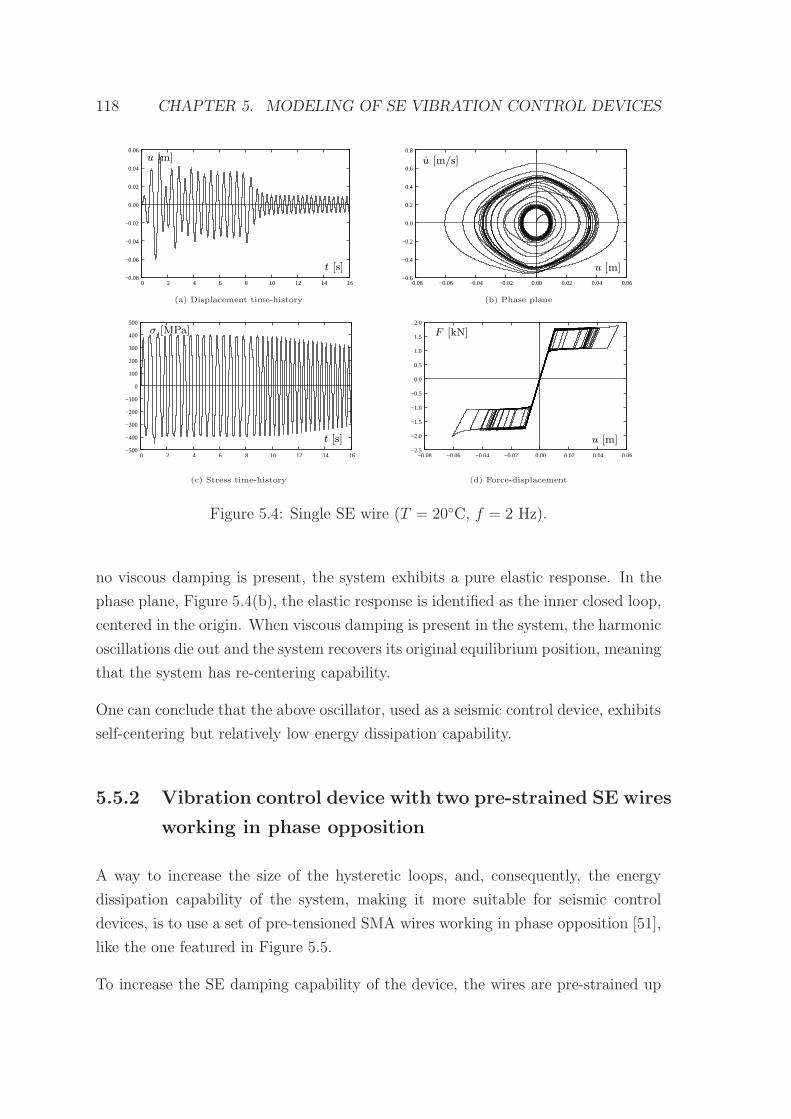
118 CHAPTER 5. MODELING OF SE VIBRATION CONTROL DEVICES
−0.08
−0.06
−0.04
−0.02
0.00
0.02
0.04
0.06
0 2 4 6 8 10 12 14 16
t [s]
u [m]
−0.6
−0.4
−0.2
0.0
0.2
0.4
0.6
0.8
−0.08 −0.06 −0.04 −0.02 0.00 0.02 0.04 0.06
u [m/s]
u [m]
(a) Displacement time-history (b) Phase plane
−500
−400
−300
−200
−100
0
100
200
300
400
500
0 2 4 6 8 10 12 14 16
t [s]
σ [MPa]
−2.5
−2.0
−1.5
−1.0
−0.5
0.0
0.5
1.0
1.5
2.0
−0.08 −0.06 −0.04 −0.02 0.00 0.02 0.04 0.06
u [m]
F [kN]
(c) Stress time-history (d) Force-displacement
Figure 5.4: Single SE wire (T = 20C, f = 2 Hz).
no viscous damping is present, the system exhibits a pure elastic response. In the
phase plane, Figure 5.4(b), the elastic response is identified as the inner closed loop,
centered in the origin. When viscous damping is present in the system, the harmonic
oscillations die out and the system recovers its original equilibrium position, meaning
that the system has re-centering capability.
One can conclude that the above oscillator, used as a seismic control device, exhibits
self-centering but relatively low energy dissipation capability.
5.5.2 Vibration control device with two pre-strained SE wires
working in phase opposition
A way to increase the size of the hysteretic loops, and, consequently, the energy
dissipation capability of the system, making it more suitable for seismic control
devices, is to use a set of pre-tensioned SMA wires working in phase opposition [51],
like the one featured in Figure 5.5.
To increase the SE damping capability of the device, the wires are pre-strained up
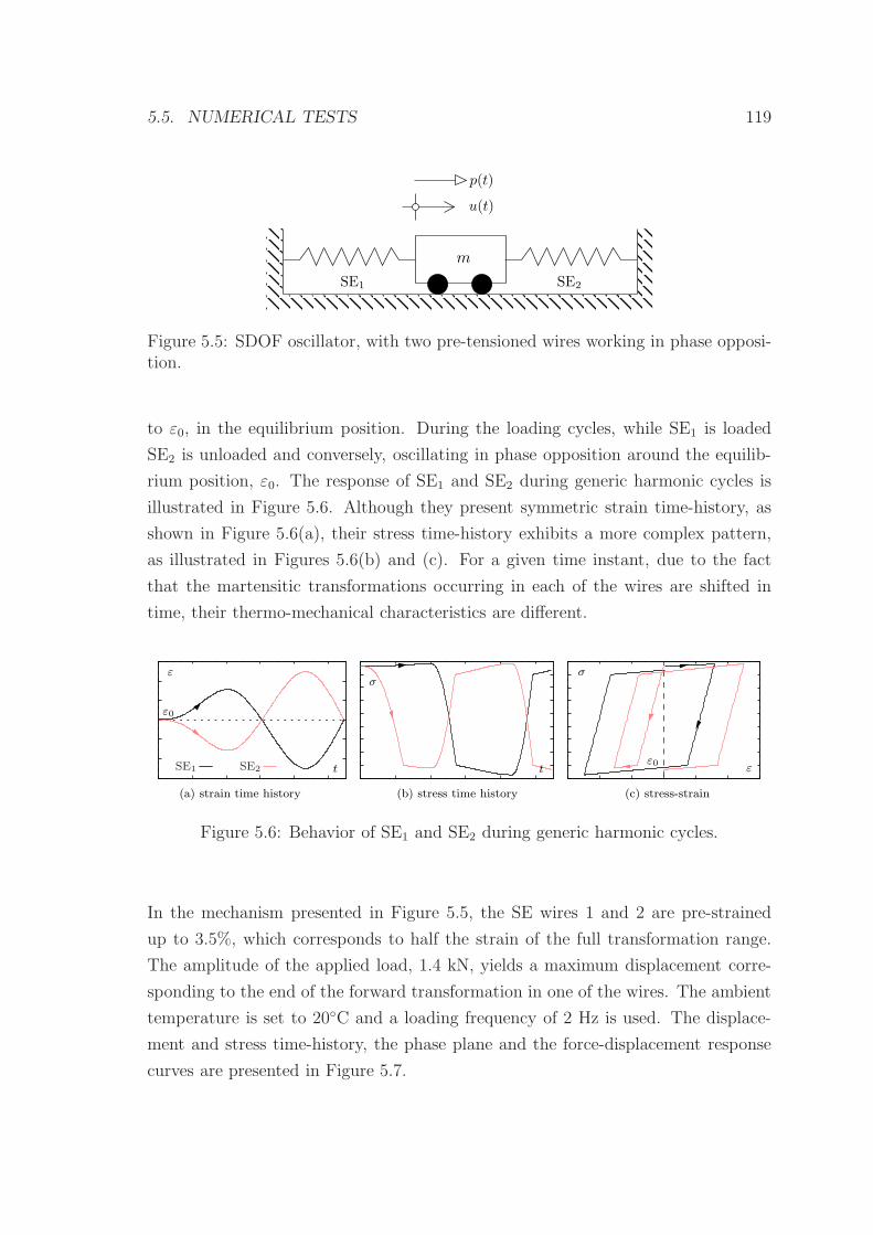
5.5. NUMERICAL TESTS 119
m
u(t)
p(t)
SE1 SE2
Figure 5.5: SDOF oscillator, with two pre-tensioned wires working in phase opposi-tion.
to ε0, in the equilibrium position. During the loading cycles, while SE1 is loaded
SE2 is unloaded and conversely, oscillating in phase opposition around the equilib-
rium position, ε0. The response of SE1 and SE2 during generic harmonic cycles is
illustrated in Figure 5.6. Although they present symmetric strain time-history, as
shown in Figure 5.6(a), their stress time-history exhibits a more complex pattern,
as illustrated in Figures 5.6(b) and (c). For a given time instant, due to the fact
that the martensitic transformations occurring in each of the wires are shifted in
time, their thermo-mechanical characteristics are different.
σ
t
ε0
t
ε
εε0
σ
(a) strain time history (b) stress time history (c) stress-strain
SE1 SE2
Figure 5.6: Behavior of SE1 and SE2 during generic harmonic cycles.
In the mechanism presented in Figure 5.5, the SE wires 1 and 2 are pre-strained
up to 3.5%, which corresponds to half the strain of the full transformation range.
The amplitude of the applied load, 1.4 kN, yields a maximum displacement corre-
sponding to the end of the forward transformation in one of the wires. The ambient
temperature is set to 20C and a loading frequency of 2 Hz is used. The displace-
ment and stress time-history, the phase plane and the force-displacement response
curves are presented in Figure 5.7.
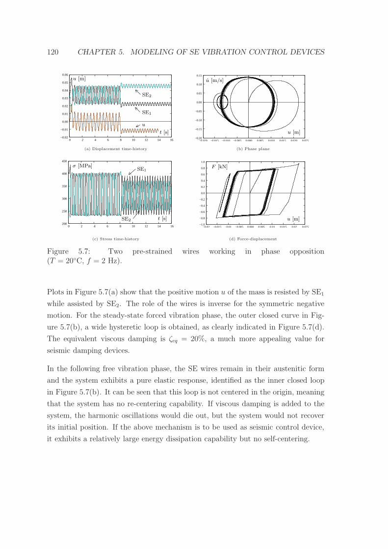
120 CHAPTER 5. MODELING OF SE VIBRATION CONTROL DEVICES
−0.02
−0.01
0.00
0.01
0.02
0.03
0.04
0.05
0.06
0 2 4 6 8 10 12 14 16
t [s]
u [m]
u
SE2
SE1
−0.20
−0.15
−0.10
−0.05
0.00
0.05
0.10
0.15
−0.020 −0.015 −0.010 −0.005 0.000 0.005 0.010 0.015 0.020 0.025
u [m]
u [m/s]
(a) Displacement time-history (b) Phase plane
200
250
300
350
400
450
0 2 4 6 8 10 12 14 16
σ [MPa]
t [s]
SE1
SE2−1.0
−0.8
−0.6
−0.4
−0.2
0.0
0.2
0.4
0.6
0.8
1.0
−0.02 −0.015 −0.01 −0.005 0.000 0.005 0.01 0.015 0.02 0.025
F [kN]
u [m]
(c) Stress time-history (d) Force-displacement
Figure 5.7: Two pre-strained wires working in phase opposition(T = 20C, f = 2 Hz).
Plots in Figure 5.7(a) show that the positive motion u of the mass is resisted by SE1
while assisted by SE2. The role of the wires is inverse for the symmetric negative
motion. For the steady-state forced vibration phase, the outer closed curve in Fig-
ure 5.7(b), a wide hysteretic loop is obtained, as clearly indicated in Figure 5.7(d).
The equivalent viscous damping is ζeq = 20%, a much more appealing value for
seismic damping devices.
In the following free vibration phase, the SE wires remain in their austenitic form
and the system exhibits a pure elastic response, identified as the inner closed loop
in Figure 5.7(b). It can be seen that this loop is not centered in the origin, meaning
that the system has no re-centering capability. If viscous damping is added to the
system, the harmonic oscillations would die out, but the system would not recover
its initial position. If the above mechanism is to be used as seismic control device,
it exhibits a relatively large energy dissipation capability but no self-centering.
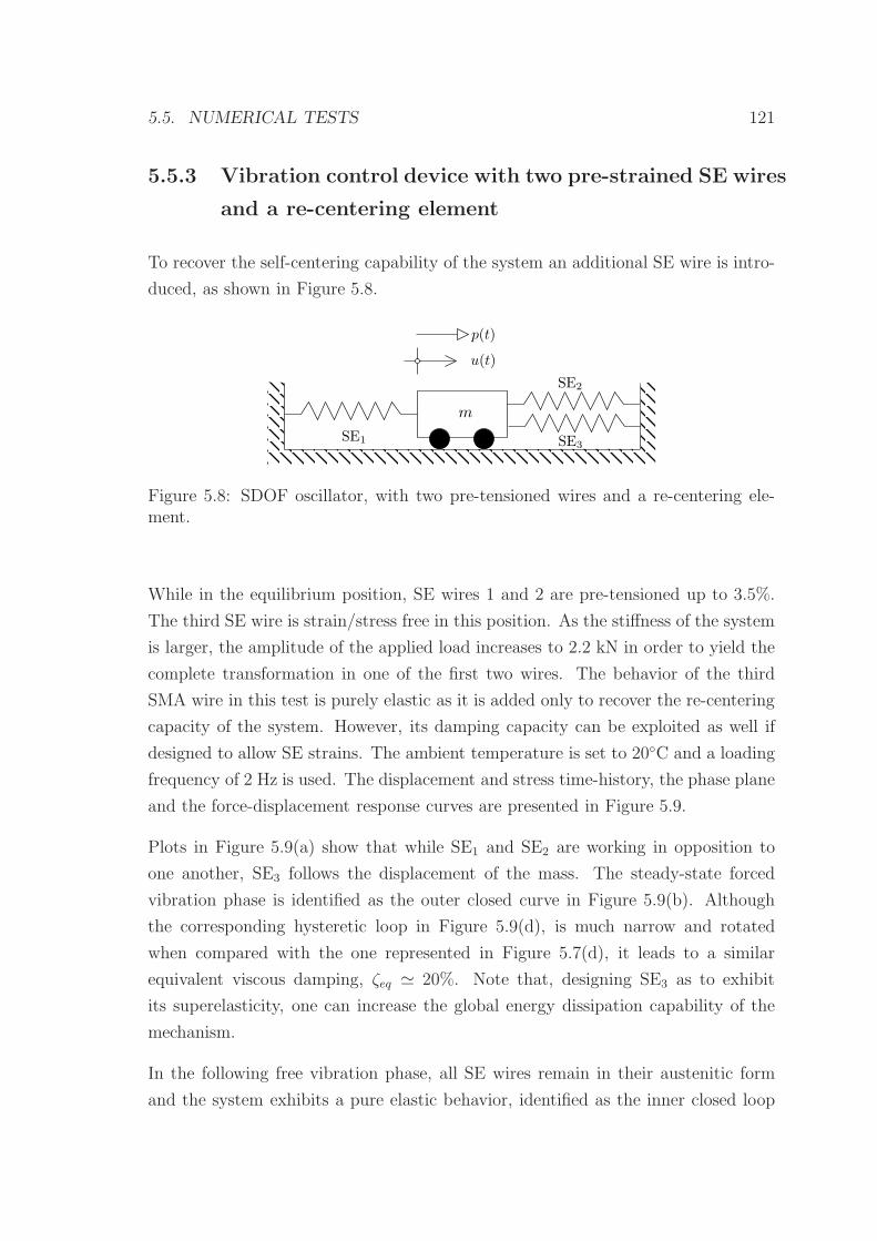
5.5. NUMERICAL TESTS 121
5.5.3 Vibration control device with two pre-strained SE wires
and a re-centering element
To recover the self-centering capability of the system an additional SE wire is intro-
duced, as shown in Figure 5.8.
m
u(t)
p(t)
SE1
SE2
SE3
Figure 5.8: SDOF oscillator, with two pre-tensioned wires and a re-centering ele-ment.
While in the equilibrium position, SE wires 1 and 2 are pre-tensioned up to 3.5%.
The third SE wire is strain/stress free in this position. As the stiffness of the system
is larger, the amplitude of the applied load increases to 2.2 kN in order to yield the
complete transformation in one of the first two wires. The behavior of the third
SMA wire in this test is purely elastic as it is added only to recover the re-centering
capacity of the system. However, its damping capacity can be exploited as well if
designed to allow SE strains. The ambient temperature is set to 20C and a loading
frequency of 2 Hz is used. The displacement and stress time-history, the phase plane
and the force-displacement response curves are presented in Figure 5.9.
Plots in Figure 5.9(a) show that while SE1 and SE2 are working in opposition to
one another, SE3 follows the displacement of the mass. The steady-state forced
vibration phase is identified as the outer closed curve in Figure 5.9(b). Although
the corresponding hysteretic loop in Figure 5.9(d), is much narrow and rotated
when compared with the one represented in Figure 5.7(d), it leads to a similar
equivalent viscous damping, ζeq ≃ 20%. Note that, designing SE3 as to exhibit
its superelasticity, one can increase the global energy dissipation capability of the
mechanism.
In the following free vibration phase, all SE wires remain in their austenitic form
and the system exhibits a pure elastic behavior, identified as the inner closed loop
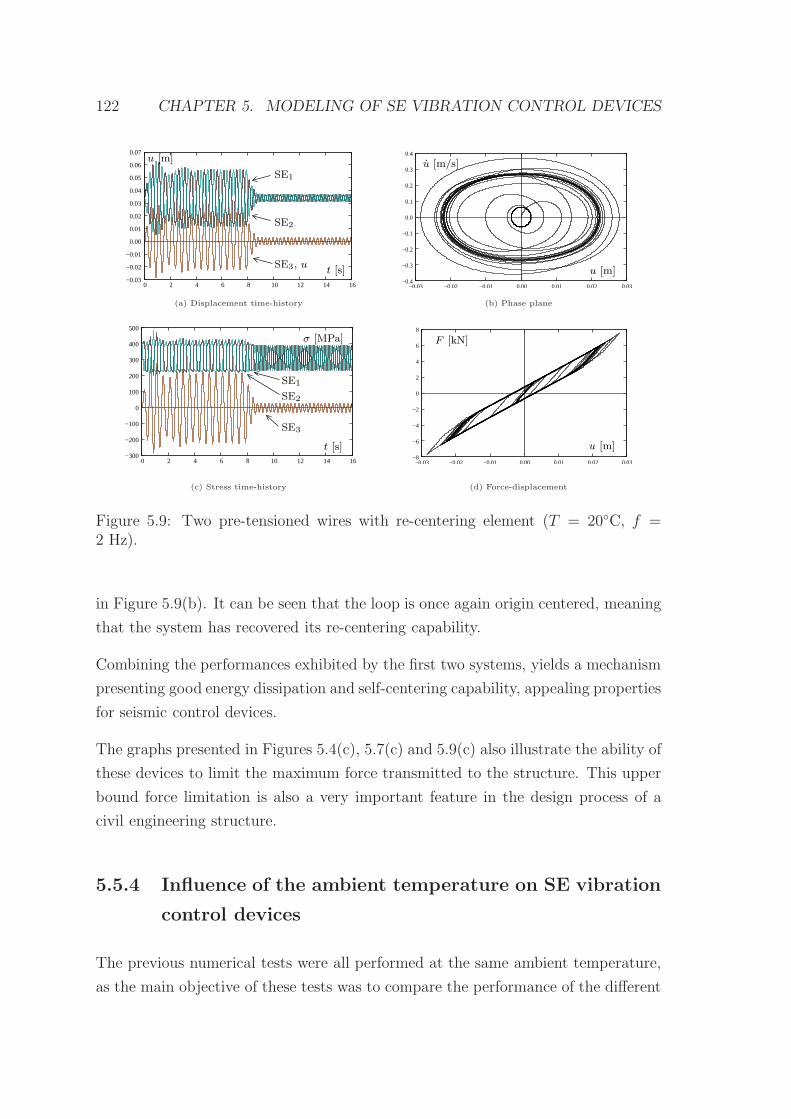
122 CHAPTER 5. MODELING OF SE VIBRATION CONTROL DEVICES
−0.03
−0.02
−0.01
0.00
0.01
0.02
0.03
0.04
0.05
0.06
0.07
0 2 4 6 8 10 12 14 16
u [m]
t [s]
SE1
SE2
SE3, u
−0.4
−0.3
−0.2
−0.1
0.0
0.1
0.2
0.3
0.4
−0.03 −0.02 −0.01 0.00 0.01 0.02 0.03
u [m/s]
u [m]
(a) Displacement time-history (b) Phase plane
−300
−200
−100
0
100
200
300
400
500
0 2 4 6 8 10 12 14 16
σ [MPa]
t [s]
SE1
SE2
SE3
−8
−6
−4
−2
0
2
4
6
8
−0.03 −0.02 −0.01 0.00 0.01 0.02 0.03
u [m]
F [kN]
(c) Stress time-history (d) Force-displacement
Figure 5.9: Two pre-tensioned wires with re-centering element (T = 20C, f =2 Hz).
in Figure 5.9(b). It can be seen that the loop is once again origin centered, meaning
that the system has recovered its re-centering capability.
Combining the performances exhibited by the first two systems, yields a mechanism
presenting good energy dissipation and self-centering capability, appealing properties
for seismic control devices.
The graphs presented in Figures 5.4(c), 5.7(c) and 5.9(c) also illustrate the ability of
these devices to limit the maximum force transmitted to the structure. This upper
bound force limitation is also a very important feature in the design process of a
civil engineering structure.
5.5.4 Influence of the ambient temperature on SE vibration
control devices
The previous numerical tests were all performed at the same ambient temperature,
as the main objective of these tests was to compare the performance of the different
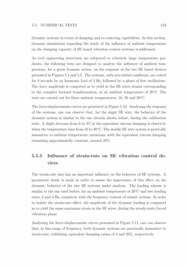
5.5. NUMERICAL TESTS 123
dynamic systems in terms of damping and re-centering capabilities. In this section,
dynamic simulations regarding the study of the influence of ambient temperature
on the damping capacity of SE based vibration control systems is addressed.
As civil engineering structures are subjected to relatively large temperature gra-
dients, the following tests are designed to analyze the influence of ambient tem-
perature, for a given dynamic action, on the response of the two SE based devices
presented in Figures 5.1 and 5.5. The systems, with zero initial conditions, are exited
for 8 seconds by an harmonic load of 2 Hz, followed by a phase of free oscillations.
The force amplitude is computed as to yield in the SE wires strains corresponding
to the complete forward transformation, at an ambient temperature of 20C. The
tests are carried out for three ambient temperatures, 10, 20 and 30C.
The force-displacements curves are presented in Figure 5.10. Analyzing the response
of the systems, one can observe that, for the single SE wire, the behavior of the
dynamic system is similar to the one already shown before, during the calibration
tests. A slight decrease from 6 to 4% in the equivalent viscous damping is observed,
when the temperature rises from 10 to 30C. The double SE wire system is pratically
insensitive to ambient temperature variations, with the equivalent viscous damping
remaining approximatelly constant, around 20%.
5.5.5 Influence of strain-rate on SE vibration control de-
vices
The strain-rate also has an important influence on the behavior of SE systems. A
parametric study is made in order to assess the importance of this effect on the
dynamic behavior of the two SE systems under analysis. The loading scheme is
similar to the one used before, for an ambient temperature of 20C and two loading
rates, 2 and 3 Hz, consistent with the frequency content of seismic actions. In order
to isolate the strain-rate effect, the amplitude of the dynamic loading is computed
as to yield the same maximum strain in the SE wires, during the steady-state forced
vibration phase.
Analyzing the force-displacements curves presented in Figure 5.11, one can observe
that, in this range of frequency, both dynamic systems are practically insensitive to
strain-rate, exhibiting equivalent damping ratios of 4 and 20%, respectively.
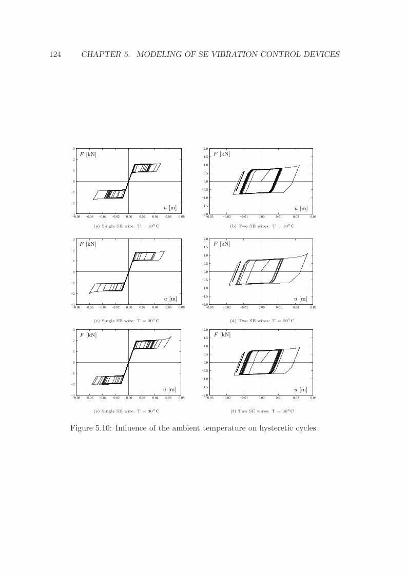
124 CHAPTER 5. MODELING OF SE VIBRATION CONTROL DEVICES
−0.08 −0.06 −0.04 −0.02 0.00 0.02 0.04 0.06 0.08
3
2
1
−1
0
−2
−3
F [kN]
u [m]−2.0
−1.5
−1.0
−0.5
0.0
0.5
1.0
1.5
2.0
−0.03 −0.02 −0.01 0.00 0.01 0.02 0.03
F [kN]
u [m]
(a) Single SE wire: T = 10C (b) Two SE wires: T = 10C
−0.08 −0.06 −0.04 −0.02 0.00 0.02 0.04 0.06 0.08
3
2
1
0
−1
−2
−3
u [m]
F [kN]
−2.0
−1.5
−1.0
−0.5
0.0
0.5
1.0
1.5
2.0
−0.03 −0.02 −0.01 0.00 0.01 0.02 0.03
u [m]
F [kN]
(c) Single SE wire: T = 20C (d) Two SE wires: T = 20C
−3
−2
−1
0
1
2
3
−0.08 −0.06 −0.04 −0.02 0.00 0.02 0.04 0.06 0.08
u [m]
F [kN]
−2.0
−1.5
−1.0
−0.5
0.0
0.5
1.0
1.5
2.0
−0.03 −0.02 −0.01 0.00 0.01 0.02 0.03
F [kN]
u [m]
(e) Single SE wire: T = 30C (f) Two SE wires: T = 30C
Figure 5.10: Influence of the ambient temperature on hysteretic cycles.
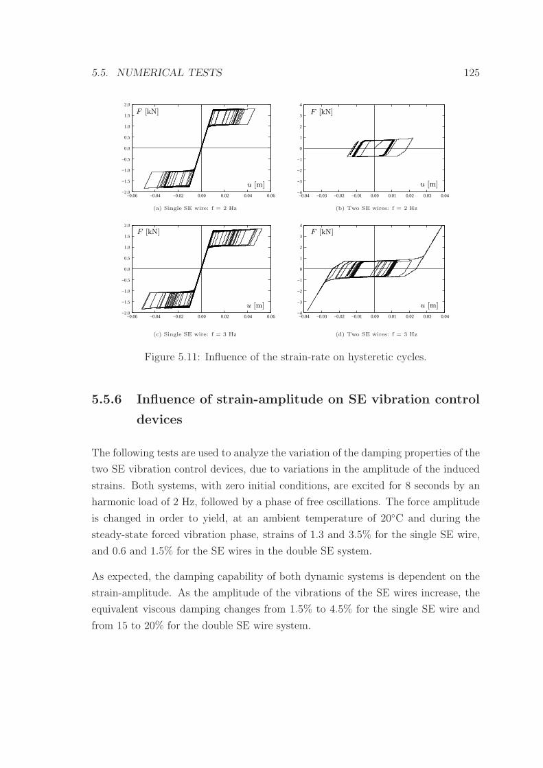
5.5. NUMERICAL TESTS 125
−2.0
−1.5
−1.0
−0.5
0.0
0.5
1.0
1.5
2.0
−0.06 −0.04 −0.02 0.00 0.02 0.04 0.06
F [kN]
u [m]−4
−3
−2
−1
0
1
2
3
4
−0.04 −0.03 −0.02 −0.01 0.00 0.01 0.02 0.03 0.04
u [m]
F [kN]
(a) Single SE wire: f = 2 Hz (b) Two SE wires: f = 2 Hz
−2.0
−1.5
−1.0
−0.5
0.0
0.5
1.0
1.5
2.0
−0.06 −0.04 −0.02 0.00 0.02 0.04 0.06
F [kN]
u [m]−4
−3
−2
−1
0
1
2
3
4
−0.04 −0.03 −0.02 −0.01 0.00 0.01 0.02 0.03 0.04
u [m]
F [kN]
(c) Single SE wire: f = 3 Hz (d) Two SE wires: f = 3 Hz
Figure 5.11: Influence of the strain-rate on hysteretic cycles.
5.5.6 Influence of strain-amplitude on SE vibration control
devices
The following tests are used to analyze the variation of the damping properties of the
two SE vibration control devices, due to variations in the amplitude of the induced
strains. Both systems, with zero initial conditions, are excited for 8 seconds by an
harmonic load of 2 Hz, followed by a phase of free oscillations. The force amplitude
is changed in order to yield, at an ambient temperature of 20C and during the
steady-state forced vibration phase, strains of 1.3 and 3.5% for the single SE wire,
and 0.6 and 1.5% for the SE wires in the double SE system.
As expected, the damping capability of both dynamic systems is dependent on the
strain-amplitude. As the amplitude of the vibrations of the SE wires increase, the
equivalent viscous damping changes from 1.5% to 4.5% for the single SE wire and
from 15 to 20% for the double SE wire system.
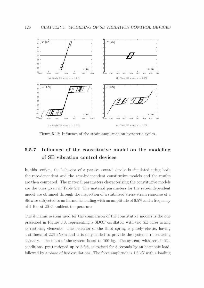
126 CHAPTER 5. MODELING OF SE VIBRATION CONTROL DEVICES
−2.0
−1.5
−1.0
−0.5
0.0
0.5
1.0
1.5
2.0
−0.06 −0.04 −0.02 0.00 0.02 0.04 0.06
u [m]
F [kN]
−4
−3
−2
−1
0
1
2
3
4
−0.04 −0.03 −0.02 −0.01 0.00 0.01 0.02 0.03 0.04
F [kN]
u [m]
(a) Single SE wire: ε = 1.5% (b) Two SE wires: ε = 0.6%
−2.0
−1.5
−1.0
−0.5
0.0
0.5
1.0
1.5
2.0
−0.06 −0.04 −0.02 0.00 0.02 0.04 0.06
u [m]
F [kN]
−4
−3
−2
−1
0
1
2
3
4
−0.04 −0.03 −0.02 −0.01 0.00 0.01 0.02 0.03 0.04
F [kN]
u [m]
(c) Single SE wire: ε = 3.5% (d) Two SE wires: ε = 1.5%
Figure 5.12: Influence of the strain-amplitude on hysteretic cycles.
5.5.7 Influence of the constitutive model on the modeling
of SE vibration control devices
In this section, the behavior of a passive control device is simulated using both
the rate-dependent and the rate-independent constitutive models and the results
are then compared. The material parameters characterizing the constitutive models
are the ones given in Table 5.1. The material parameters for the rate-independent
model are obtained through the inspection of a stabilized stress-strain response of a
SE wire subjected to an harmonic loading with an amplitude of 6.5% and a frequency
of 1 Hz, at 20C ambient temperature.
The dynamic system used for the comparison of the constitutive models is the one
presented in Figure 5.8, representing a SDOF oscillator, with two SE wires acting
as restoring elements. The behavior of the third spring is purely elastic, having
a stiffness of 226 kN/m and it is only added to provide the system’s re-centering
capacity. The mass of the system is set to 100 kg. The system, with zero initial
conditions, pre-tensioned up to 3.5%, is excited for 8 seconds by an harmonic load,
followed by a phase of free oscillations. The force amplitude is 1.6 kN with a loading
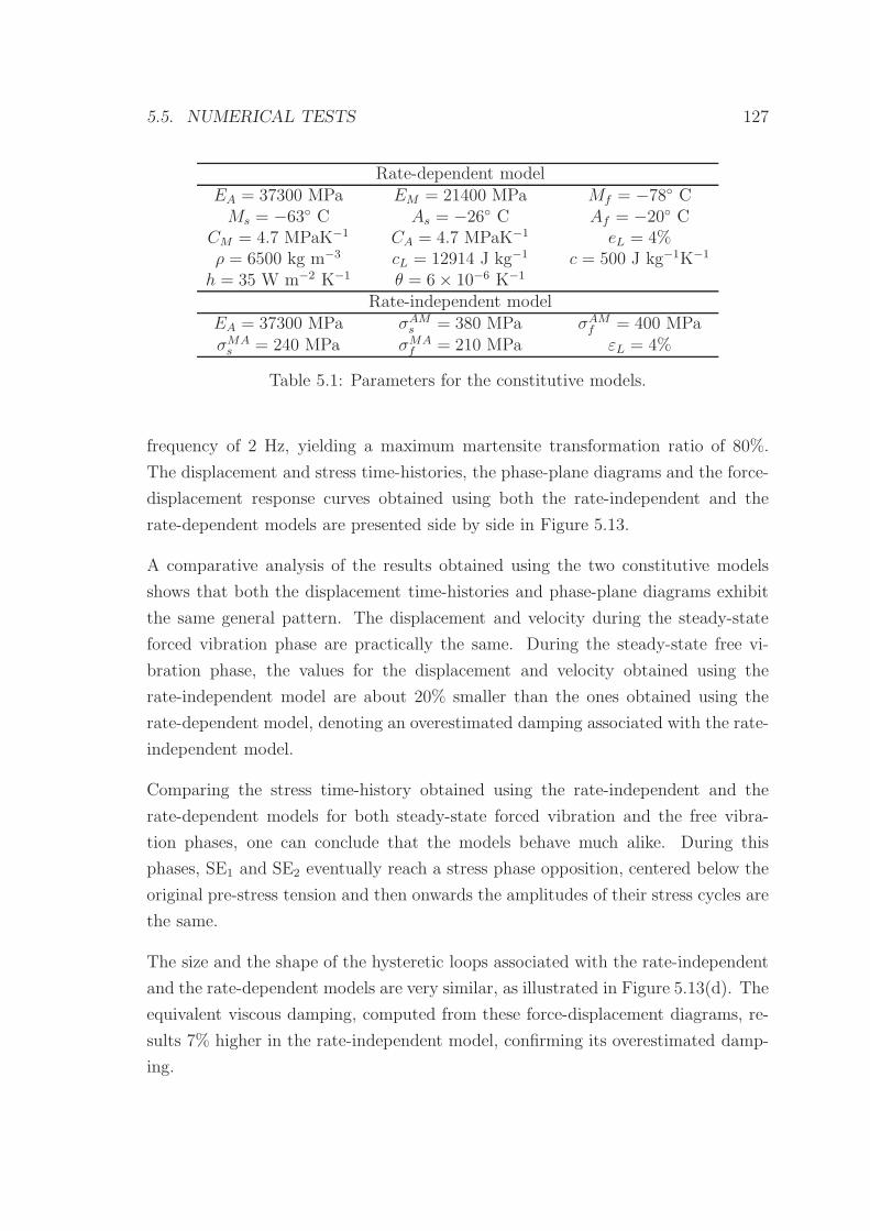
5.5. NUMERICAL TESTS 127
Rate-dependent modelEA = 37300 MPa EM = 21400 MPa Mf = −78 CMs = −63 C As = −26 C Af = −20 C
CM = 4.7 MPaK−1 CA = 4.7 MPaK−1 eL = 4%ρ = 6500 kg m−3 cL = 12914 J kg−1 c = 500 J kg−1K−1
h = 35 W m−2 K−1 θ = 6× 10⁻⁶ K−1
Rate-independent modelEA = 37300 MPa σAM
s = 380 MPa σAMf = 400 MPa
σMAs = 240 MPa σMA
f = 210 MPa εL = 4%
Table 5.1: Parameters for the constitutive models.
frequency of 2 Hz, yielding a maximum martensite transformation ratio of 80%.
The displacement and stress time-histories, the phase-plane diagrams and the force-
displacement response curves obtained using both the rate-independent and the
rate-dependent models are presented side by side in Figure 5.13.
A comparative analysis of the results obtained using the two constitutive models
shows that both the displacement time-histories and phase-plane diagrams exhibit
the same general pattern. The displacement and velocity during the steady-state
forced vibration phase are practically the same. During the steady-state free vi-
bration phase, the values for the displacement and velocity obtained using the
rate-independent model are about 20% smaller than the ones obtained using the
rate-dependent model, denoting an overestimated damping associated with the rate-
independent model.
Comparing the stress time-history obtained using the rate-independent and the
rate-dependent models for both steady-state forced vibration and the free vibra-
tion phases, one can conclude that the models behave much alike. During this
phases, SE1 and SE2 eventually reach a stress phase opposition, centered below the
original pre-stress tension and then onwards the amplitudes of their stress cycles are
the same.
The size and the shape of the hysteretic loops associated with the rate-independent
and the rate-dependent models are very similar, as illustrated in Figure 5.13(d). The
equivalent viscous damping, computed from these force-displacement diagrams, re-
sults 7% higher in the rate-independent model, confirming its overestimated damp-
ing.
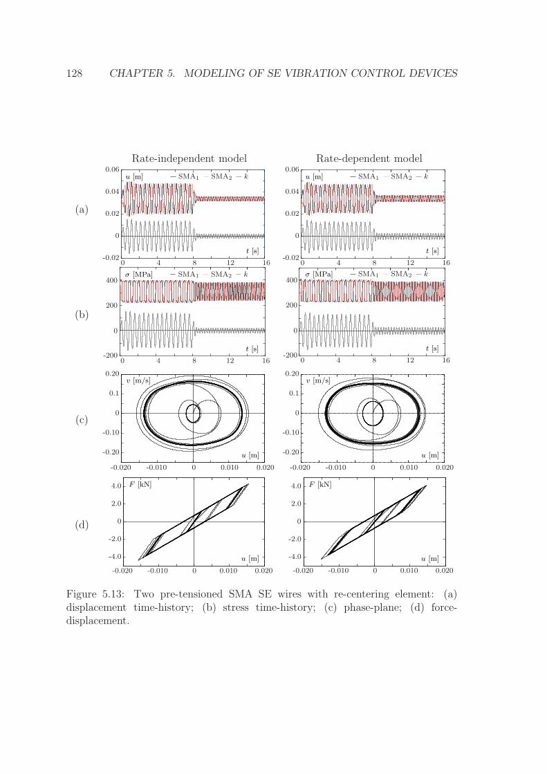
128 CHAPTER 5. MODELING OF SE VIBRATION CONTROL DEVICES
(a)
Rate-independent model
u [m]
t [s]-0.02
0
0.02
0.04
0.06SMA1 SMA2 k
0 4 8 12 16
Rate-dependent model
u [m]
t [s]-0.02
0
0.02
0.04
0.06SMA1 SMA2 k
0 4 8 12 16
(b)
σ [MPa]
t [s]
SMA1 SMA2 k
-200
200
400
0
0 4 8 12 16
σ [MPa]
t [s]
SMA1 SMA2 k
-200
200
400
0
0 4 8 12 16
(c)
v [m/s]
u [m]
-0.010 0-0.020 0.010 0.020
0
0.1
0.20
-0.20
-0.10
v [m/s]
u [m]
-0.010 0-0.020 0.010 0.020
0
0.1
0.20
-0.20
-0.10
(d)
F [kN]
u [m]
0-0.020 -0.010 0.010 0.020
0
4.0
2.0
-2.0
-4.0
F [kN]
u [m]
0-0.020 -0.010 0.010 0.020
0
4.0
2.0
-2.0
-4.0
Figure 5.13: Two pre-tensioned SMA SE wires with re-centering element: (a)displacement time-history; (b) stress time-history; (c) phase-plane; (d) force-displacement.
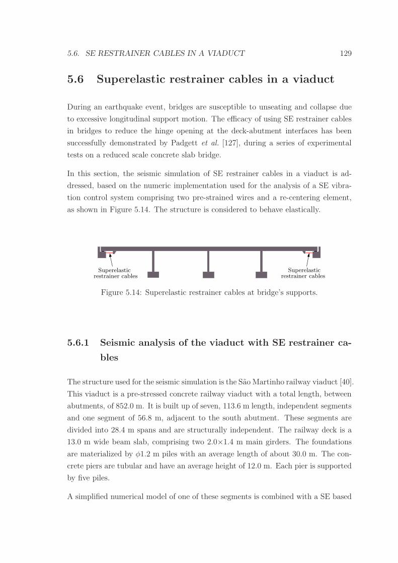
5.6. SE RESTRAINER CABLES IN A VIADUCT 129
5.6 Superelastic restrainer cables in a viaduct
During an earthquake event, bridges are susceptible to unseating and collapse due
to excessive longitudinal support motion. The efficacy of using SE restrainer cables
in bridges to reduce the hinge opening at the deck-abutment interfaces has been
successfully demonstrated by Padgett et al. [127], during a series of experimental
tests on a reduced scale concrete slab bridge.
In this section, the seismic simulation of SE restrainer cables in a viaduct is ad-
dressed, based on the numeric implementation used for the analysis of a SE vibra-
tion control system comprising two pre-strained wires and a re-centering element,
as shown in Figure 5.14. The structure is considered to behave elastically.
Superelasticrestrainer cables
Superelasticrestrainer cables
Figure 5.14: Superelastic restrainer cables at bridge’s supports.
5.6.1 Seismic analysis of the viaduct with SE restrainer ca-
bles
The structure used for the seismic simulation is the Sao Martinho railway viaduct [40].
This viaduct is a pre-stressed concrete railway viaduct with a total length, between
abutments, of 852.0 m. It is built up of seven, 113.6 m length, independent segments
and one segment of 56.8 m, adjacent to the south abutment. These segments are
divided into 28.4 m spans and are structurally independent. The railway deck is a
13.0 m wide beam slab, comprising two 2.0×1.4 m main girders. The foundations
are materialized by φ1.2 m piles with an average length of about 30.0 m. The con-
crete piers are tubular and have an average height of 12.0 m. Each pier is supported
by five piles.
A simplified numerical model of one of these segments is combined with a SE based
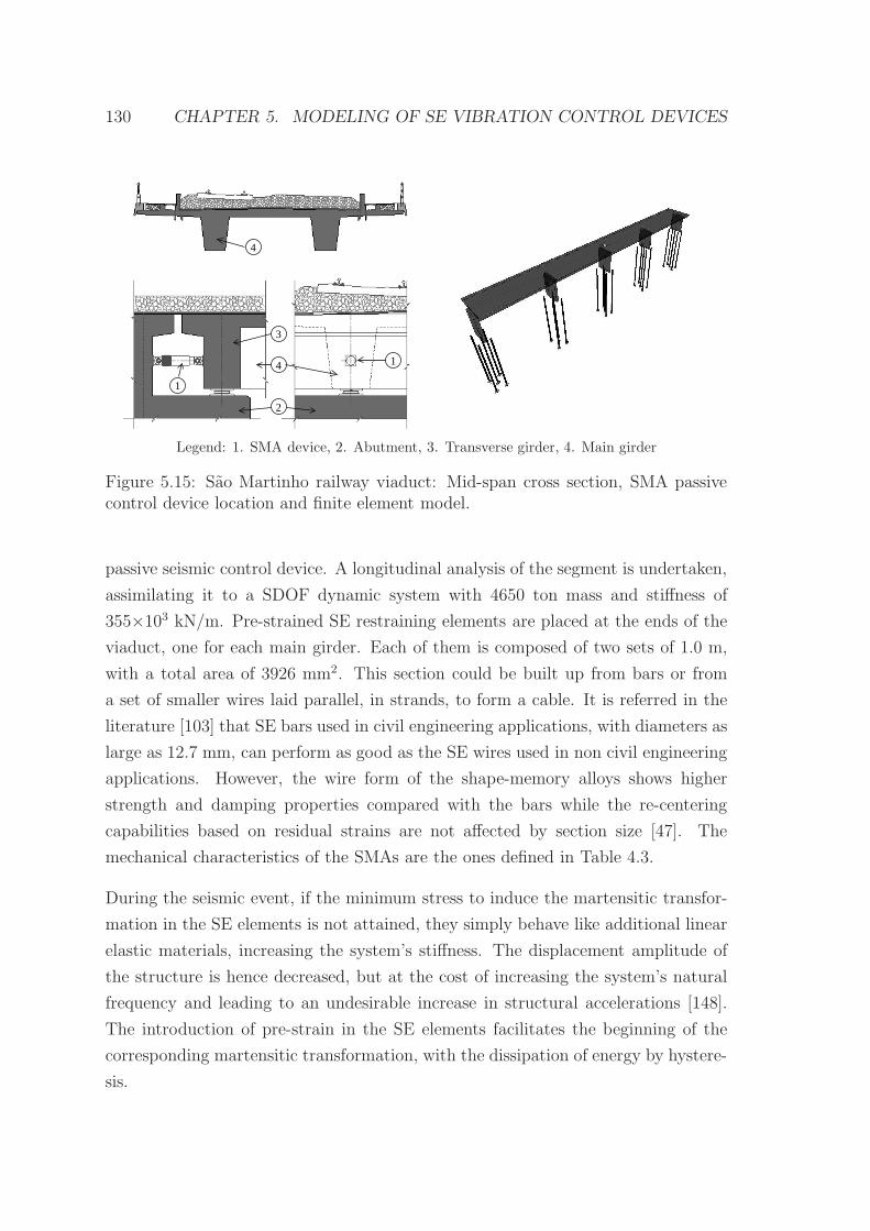
130 CHAPTER 5. MODELING OF SE VIBRATION CONTROL DEVICES
1
3
4
2
4
1
Legend: 1. SMA device, 2. Abutment, 3. Transverse girder, 4. Main girder
Figure 5.15: Sao Martinho railway viaduct: Mid-span cross section, SMA passivecontrol device location and finite element model.
passive seismic control device. A longitudinal analysis of the segment is undertaken,
assimilating it to a SDOF dynamic system with 4650 ton mass and stiffness of
355×103 kN/m. Pre-strained SE restraining elements are placed at the ends of the
viaduct, one for each main girder. Each of them is composed of two sets of 1.0 m,
with a total area of 3926 mm2. This section could be built up from bars or from
a set of smaller wires laid parallel, in strands, to form a cable. It is referred in the
literature [103] that SE bars used in civil engineering applications, with diameters as
large as 12.7 mm, can perform as good as the SE wires used in non civil engineering
applications. However, the wire form of the shape-memory alloys shows higher
strength and damping properties compared with the bars while the re-centering
capabilities based on residual strains are not affected by section size [47]. The
mechanical characteristics of the SMAs are the ones defined in Table 4.3.
During the seismic event, if the minimum stress to induce the martensitic transfor-
mation in the SE elements is not attained, they simply behave like additional linear
elastic materials, increasing the system’s stiffness. The displacement amplitude of
the structure is hence decreased, but at the cost of increasing the system’s natural
frequency and leading to an undesirable increase in structural accelerations [148].
The introduction of pre-strain in the SE elements facilitates the beginning of the
corresponding martensitic transformation, with the dissipation of energy by hystere-
sis.
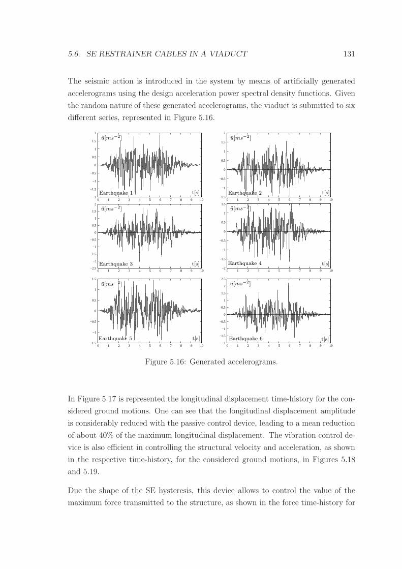
5.6. SE RESTRAINER CABLES IN A VIADUCT 131
The seismic action is introduced in the system by means of artificially generated
accelerograms using the design acceleration power spectral density functions. Given
the random nature of these generated accelerograms, the viaduct is submitted to six
different series, represented in Figure 5.16.
−2
−1.5
−1
−0.5
0
0.5
1
1.5
2
0 1 2 3 4 5 6 7 8 9 10
u[ms−2]
Earthquake 1 t[s]−1.5
−1
−0.5
0
0.5
1
1.5
2
0 1 2 3 4 5 6 7 8 9 10
t[s]
u[ms−2]
Earthquake 2
−2.5
−2
−1.5
−1
−0.5
0
0.5
1
1.5
2
0 1 2 3 4 5 6 7 8 9 10
u[ms−2]
t[s]Earthquake 3−2
−1.5
−1
−0.5
0
0.5
1
1.5
0 1 2 3 4 5 6 7 8 9 10
u[ms−2]
t[s]Earthquake 4
−1.5
−1
−0.5
0
0.5
1
1.5
0 1 2 3 4 5 6 7 8 9 10
u[ms−2]
t[s]Earthquake 5−2
−1.5
−1
−0.5
0
0.5
1
1.5
2
2.5
0 1 2 3 4 5 6 7 8 9 10
t[s]Earthquake 6
u[ms−2]
Figure 5.16: Generated accelerograms.
In Figure 5.17 is represented the longitudinal displacement time-history for the con-
sidered ground motions. One can see that the longitudinal displacement amplitude
is considerably reduced with the passive control device, leading to a mean reduction
of about 40% of the maximum longitudinal displacement. The vibration control de-
vice is also efficient in controlling the structural velocity and acceleration, as shown
in the respective time-history, for the considered ground motions, in Figures 5.18
and 5.19.
Due the shape of the SE hysteresis, this device allows to control the value of the
maximum force transmitted to the structure, as shown in the force time-history for
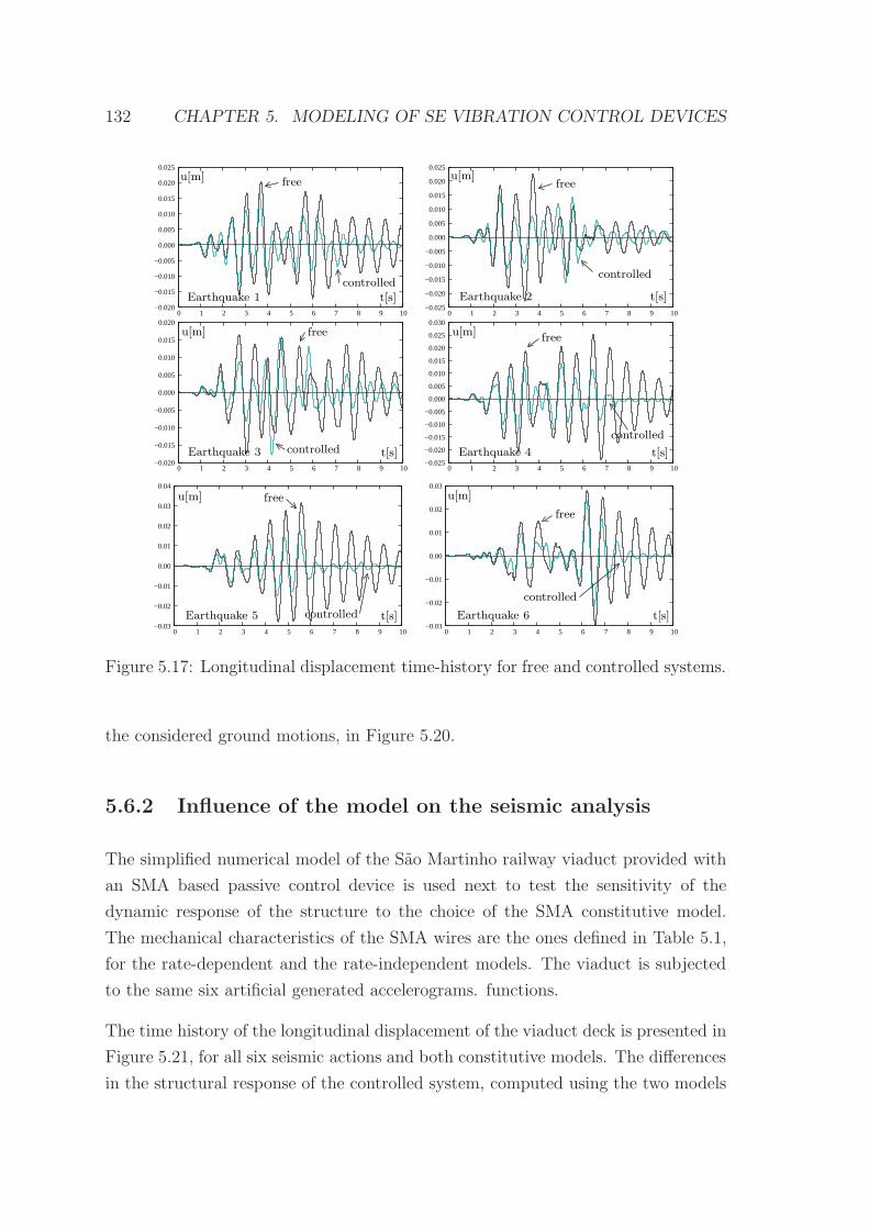
132 CHAPTER 5. MODELING OF SE VIBRATION CONTROL DEVICES
−0.020
−0.015
−0.010
−0.005
0.000
0.005
0.010
0.015
0.020
0.025
0 1 2 3 4 5 6 7 8 9 10
free
controlledEarthquake 1 t[s]
u[m]
−0.025
−0.020
−0.015
−0.010
−0.005
0.000
0.005
0.010
0.015
0.020
0.025
0 1 2 3 4 5 6 7 8 9 10
t[s]
u[m]
Earthquake 2
controlled
free
−0.020
−0.015
−0.010
−0.005
0.000
0.005
0.010
0.015
0.020
0 1 2 3 4 5 6 7 8 9 10
t[s]
u[m]
Earthquake 3 controlled
free
−0.025
−0.020
−0.015
−0.010
−0.005
0.000
0.005
0.010
0.015
0.020
0.025
0.030
0 1 2 3 4 5 6 7 8 9 10
t[s]
u[m]
Earthquake 4
free
controlled
−0.03
−0.02
−0.01
0.00
0.01
0.02
0.03
0.04
0 1 2 3 4 5 6 7 8 9 10
Earthquake 5
free
controlled t[s]
u[m]
−0.03
−0.02
−0.01
0.00
0.01
0.02
0.03
0 1 2 3 4 5 6 7 8 9 10
Earthquake 6
free
controlled
t[s]
u[m]
Figure 5.17: Longitudinal displacement time-history for free and controlled systems.
the considered ground motions, in Figure 5.20.
5.6.2 Influence of the model on the seismic analysis
The simplified numerical model of the Sao Martinho railway viaduct provided with
an SMA based passive control device is used next to test the sensitivity of the
dynamic response of the structure to the choice of the SMA constitutive model.
The mechanical characteristics of the SMA wires are the ones defined in Table 5.1,
for the rate-dependent and the rate-independent models. The viaduct is subjected
to the same six artificial generated accelerograms. functions.
The time history of the longitudinal displacement of the viaduct deck is presented in
Figure 5.21, for all six seismic actions and both constitutive models. The differences
in the structural response of the controlled system, computed using the two models
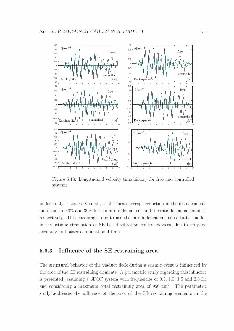
5.6. SE RESTRAINER CABLES IN A VIADUCT 133
−0.2
−0.15
−0.1
−0.05
0
0.05
0.1
0.15
0.2
0.25
0 1 2 3 4 5 6 7 8 9 10
t[s]
u[ms−1]free
controlled
Earthquake 1−0.2
−0.15
−0.1
−0.05
0
0.05
0.1
0.15
0.2
0 1 2 3 4 5 6 7 8 9 10
t[s]
u[ms−1]free
controlled
Earthquake 2
−0.2
−0.15
−0.1
−0.05
0
0.05
0.1
0.15
0.2
0 1 2 3 4 5 6 7 8 9 10
t[s]
u[ms−1]free
controlledEarthquake 3−0.25
−0.2
−0.15
−0.1
−0.05
0
0.05
0.1
0.15
0.2
0.25
0 1 2 3 4 5 6 7 8 9 10
t[s]
u[ms−1] free
controlledEarthquake 4
−0.25
−0.2
−0.15
−0.1
−0.05
0
0.05
0.1
0.15
0.2
0.25
0 1 2 3 4 5 6 7 8 9 10
t[s]
u[ms−1]free
controlledEarthquake 5
−0.3
−0.2
−0.1
0
0.1
0.2
0.3
0 1 2 3 4 5 6 7 8 9 10
t[s]
u[ms−1] free
controlledEarthquake 6
Figure 5.18: Longitudinal velocity time-history for free and controlledsystems.
under analysis, are very small, as the mean average reduction in the displacements
amplitude is 33% and 30% for the rate-independent and the rate-dependent models,
respectively. This encourages one to use the rate-independent constitutive model,
in the seismic simulation of SE based vibration control devices, due to its good
accuracy and faster computational time.
5.6.3 Influence of the SE restraining area
The structural behavior of the viaduct deck during a seismic event is influenced by
the area of the SE restraining elements. A parametric study regarding this influence
is presented, assuming a SDOF system with frequencies of 0.5, 1.0, 1.5 and 2.0 Hz
and considering a maximum total restraining area of 950 cm2. The parametric
study addresses the influence of the area of the SE restraining elements in the
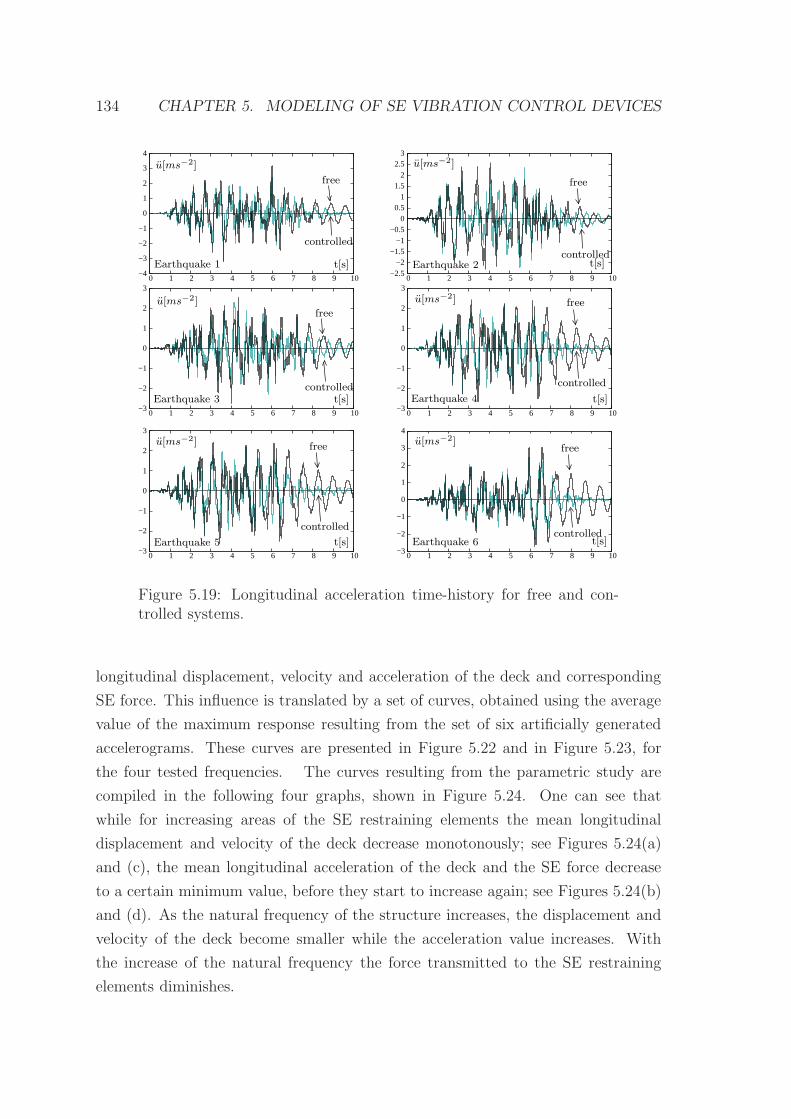
134 CHAPTER 5. MODELING OF SE VIBRATION CONTROL DEVICES
−4
−3
−2
−1
0
1
2
3
4
0 1 2 3 4 5 6 7 8 9 10
t[s]Earthquake 1
free
controlled
u[ms−2]
−2.5−2
−1.5−1
−0.5 0
0.5 1
1.5 2
2.5 3
0 1 2 3 4 5 6 7 8 9 10
t[s]Earthquake 2
free
controlled
u[ms−2]
−3
−2
−1
0
1
2
3
0 1 2 3 4 5 6 7 8 9 10
t[s]Earthquake 3
free
controlled
u[ms−2]
−3
−2
−1
0
1
2
3
0 1 2 3 4 5 6 7 8 9 10
u[ms−2]
t[s]Earthquake 4
free
controlled
−3
−2
−1
0
1
2
3
0 1 2 3 4 5 6 7 8 9 10
t[s]Earthquake 5
free
controlled
u[ms−2]
−3
−2
−1
0
1
2
3
4
0 1 2 3 4 5 6 7 8 9 10
t[s]Earthquake 6
free
controlled
u[ms−2]
Figure 5.19: Longitudinal acceleration time-history for free and con-trolled systems.
longitudinal displacement, velocity and acceleration of the deck and corresponding
SE force. This influence is translated by a set of curves, obtained using the average
value of the maximum response resulting from the set of six artificially generated
accelerograms. These curves are presented in Figure 5.22 and in Figure 5.23, for
the four tested frequencies. The curves resulting from the parametric study are
compiled in the following four graphs, shown in Figure 5.24. One can see that
while for increasing areas of the SE restraining elements the mean longitudinal
displacement and velocity of the deck decrease monotonously; see Figures 5.24(a)
and (c), the mean longitudinal acceleration of the deck and the SE force decrease
to a certain minimum value, before they start to increase again; see Figures 5.24(b)
and (d). As the natural frequency of the structure increases, the displacement and
velocity of the deck become smaller while the acceleration value increases. With
the increase of the natural frequency the force transmitted to the SE restraining
elements diminishes.
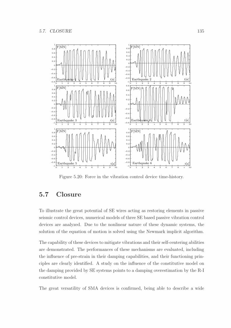
5.7. CLOSURE 135
1
0.8
0.6
0.4
0.2
0
-0.2
-0.4
-0.6
-0.80 1 2 3 4 5 6 7 8 9 10
Earthquake 1 t[s]
F[MN]1
0.8
0.6
0.4
0.2
0
-0.2
-0.4
-0.6
-0.8
-1109876543210
Earthquake 2 t[s]
F[MN]
1
0.8
0.6
0.4
0.2
0
-0.2
-0.4
-0.6
-0.8
-10 1 2 3 4 5 6 7 8 9 10
Earthquake 3 t[s]
F[MN]
4
0.8
0.6
0.4
0.2
0
-0.2
-0.4
-0.6
-0.80 1 2 3 5 6 7 8 9 10
Earthquake 4 t[s]
F[MN]
0.8
1
0.6
0.4
0.2
0
-0.2
-0.4
-0.6
-0.8
-10 1 2 3 4 5 6 7 8 9 10
Earthquake 5 t[s]
F[MN]
9
1
0.8
0.6
0.4
0.2
0
-0.2
-0.4
-0.6
-0.8
-10 1 2 3 4 5 6 7 8 10
Earthquake 6 t[s]
F[MN]
Figure 5.20: Force in the vibration control device time-history.
5.7 Closure
To illustrate the great potential of SE wires acting as restoring elements in passive
seismic control devices, numerical models of three SE based passive vibration control
devices are analyzed. Due to the nonlinear nature of these dynamic systems, the
solution of the equation of motion is solved using the Newmark implicit algorithm.
The capability of these devices to mitigate vibrations and their self-centering abilities
are demonstrated. The performances of these mechanisms are evaluated, including
the influence of pre-strain in their damping capabilities, and their functioning prin-
ciples are clearly identified. A study on the influence of the constitutive model on
the damping provided by SE systems points to a damping overestimation by the R-I
constitutive model.
The great versatility of SMA devices is confirmed, being able to describe a wide
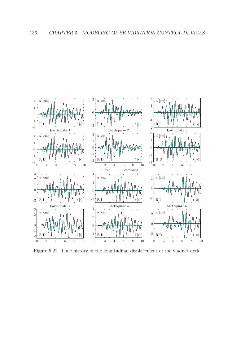
136 CHAPTER 5. MODELING OF SE VIBRATION CONTROL DEVICES
−2
−2
u [cm] u [cm] u [cm]
Earthquake 6Earthquake 5Earthquake 4
R-I R-I R-It [s] t [s] t [s]
R-D R-D R-Dt [s] t [s] t [s]
u [cm] u [cm] u [cm]
u [cm] u [cm] u [cm]
t [s] t [s] t [s]
t [s] t [s] t [s]
u [cm] u [cm] u [cm]
Earthquake 1 Earthquake 2 Earthquake 3
R-I R-I R-I
R-D R-D R-D
-2
-1
0
1
2
2
1
0
-1
-2
2
1
0
-1
-2
2
1
0
-1
-2
-2
-1
0
1
2
-2
-1
0
1
2
-2
2
0
-2
0
2
4
-2
0
2
4
-2
0
2
0
2
3
1
-1
0
2
3
1
-1
0 2 4 6 8 10 0 2 4 6 8 100 2 4 6 8 10
0 2 4 6 8 10 0 2 4 6 8 10 0 2 4 6 8 10
controledfree
Figure 5.21: Time history of the longitudinal displacement of the viaduct deck.
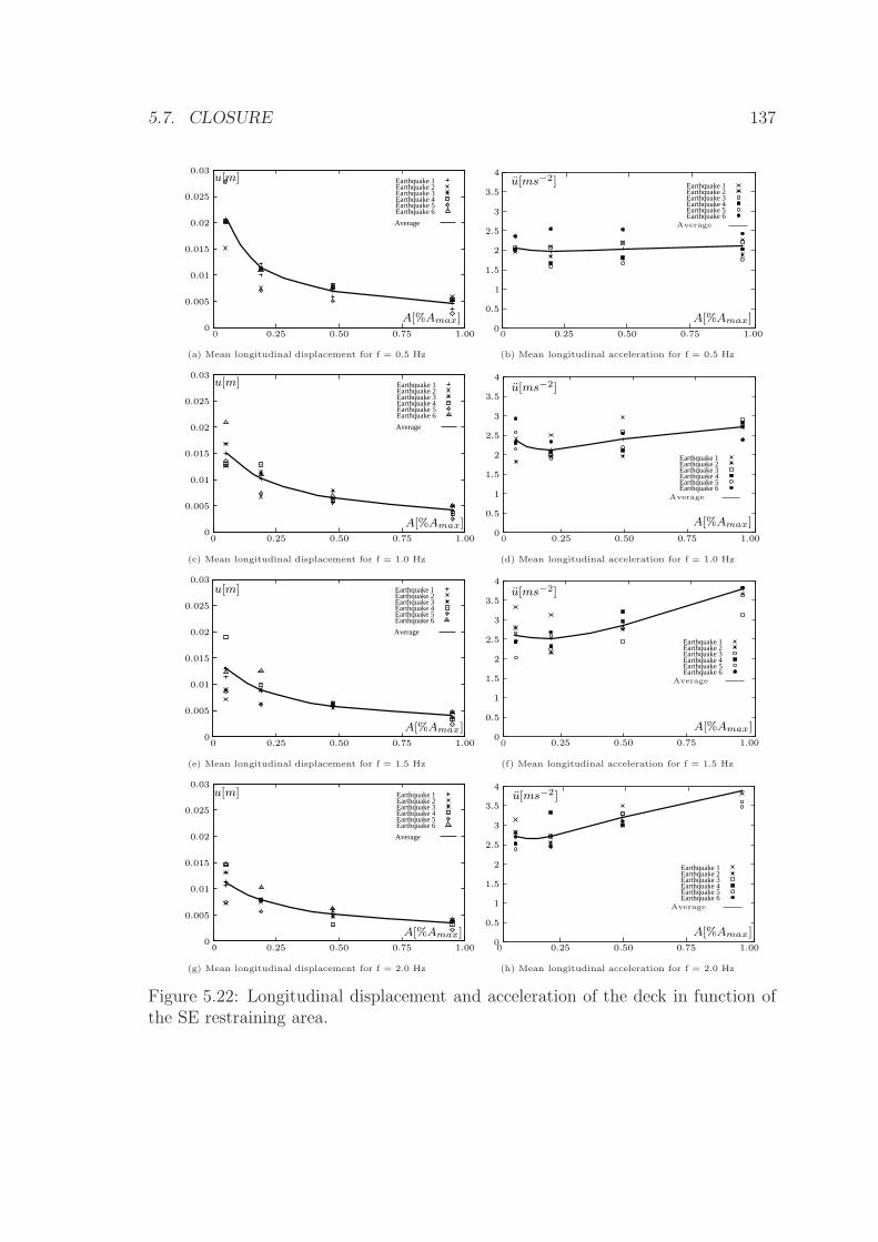
5.7. CLOSURE 137
Earthquake 1Earthquake 2Earthquake 3Earthquake 4Earthquake 5Earthquake 6
Average
0.03
0.025
0.02
0.015
0.01
0.005
0
u[m]
0.25 0.75 1.00
A[%Amax]
0.500
Earthquake 2Earthquake 3Earthquake 4Earthquake 5Earthquake 6
Earthquake 1
1
A[%Amax]
0.25 0.50 0.75 1.00
4
3.5
3
2.5
2
1.5
0.5
0
u[ms−2]
Average
0
(a) Mean longitudinal displacement for f = 0.5 Hz (b) Mean longitudinal acceleration for f = 0.5 Hz
Earthquake 1Earthquake 2Earthquake 3Earthquake 4Earthquake 5Earthquake 6
Average
A[%Amax]
0.03
0.025
0.02
0.015
0.01
0.005
00
u[m]
1.000.500.25 0.75
Earthquake 2Earthquake 3Earthquake 4Earthquake 5Earthquake 6
Earthquake 1
A[%Amax]
4
3.5
3
2.5
2
1.5
1
0.5
0
u[ms−2]
1.000.750.500.25
Average
0
(c) Mean longitudinal displacement for f = 1.0 Hz (d) Mean longitudinal acceleration for f = 1.0 Hz
Earthquake 1Earthquake 2Earthquake 3Earthquake 4Earthquake 5Earthquake 6
Average
A[%Amax]
0.03
0.025
0.02
0.015
0.01
0.005
00
u[m]
1.000.750.500.25
Earthquake 2Earthquake 3Earthquake 4Earthquake 5Earthquake 6
Earthquake 1
A[%Amax]
4
3.5
3
2.5
2
1.5
1
0.5
0
u[ms−2]
1.000.750.500.25
Average
0
(e) Mean longitudinal displacement for f = 1.5 Hz (f) Mean longitudinal acceleration for f = 1.5 Hz
Earthquake 1Earthquake 2Earthquake 3Earthquake 4Earthquake 5Earthquake 6
Average
0
A[%Amax]
0.03
0.025
0.02
0.015
0.01
0.005
0
u[m]
0.75 1.000.500.25
Earthquake 2Earthquake 3Earthquake 4Earthquake 5Earthquake 6
Earthquake 1
A[%Amax]
0.25 0.50 0.75 1.00
4
3.5
3
2.5
2
1.5
1
0.5
0
u[ms−2]
Average
0
(g) Mean longitudinal displacement for f = 2.0 Hz (h) Mean longitudinal acceleration for f = 2.0 Hz
Figure 5.22: Longitudinal displacement and acceleration of the deck in function ofthe SE restraining area.
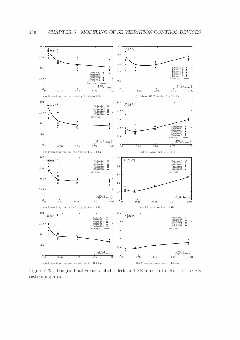
138 CHAPTER 5. MODELING OF SE VIBRATION CONTROL DEVICES
Earthquake 2Earthquake 3Earthquake 4Earthquake 5Earthquake 6
Earthquake 1
A[%Amax]
0.2
0.15
0.1
0.05
0
u[ms−1]
1.000.750.500.25
Average
0
Earthquake 2Earthquake 3Earthquake 4Earthquake 5Earthquake 6
Earthquake 1
0.25 0.50 0.75 1.00
A[%Amax]0
2.5
2.0
1.5
1.0
0.5
F [MN ]
Average
0
(a) Mean longitudinal velocity for f = 0.5 Hz (b) Mean SE Force for f = 0.5 Hz
Earthquake 2Earthquake 3Earthquake 4Earthquake 5Earthquake 6
Earthquake 1
A[%Amax]
0.2
0.15
0.05
0
0.1
u[ms−1]
1.000.750.500.25
Average
0
Earthquake 2Earthquake 3Earthquake 4Earthquake 5Earthquake 6
Earthquake 1
A[%Amax]
2.0
0
2.5
1.0
1.5
0.5
F [MN ]
1.000.750.500.25
Average
0
(c) Mean longitudinal velocity for f = 1.0 Hz (d) SE force for f = 1.0 Hz
Earthquake 2Earthquake 3Earthquake 4Earthquake 5Earthquake 6
Earthquake 1
A[%Amax]0
0.05
0.1
0.15
0.2
1.5 1.00
u[ms−1]
0.750.50
Average
0
Earthquake 2Earthquake 3Earthquake 4Earthquake 5Earthquake 6
Earthquake 1
A[%Amax]0
2.5
2.0
1.5
1.0
0.5
0.25 0.50
F [MN ]
1.000.75
Average
0
(e) Mean longitudinal velocity for f = 1.5 Hz (f) SE force for f = 1.5 Hz
Earthquake 2Earthquake 3Earthquake 4Earthquake 5Earthquake 6
Earthquake 1
A[%Amax]0
0.05
0.1
0.15
0.2
1.00
u[ms−1]
0.750.500.25
Average
0
Earthquake 2Earthquake 3Earthquake 4Earthquake 5Earthquake 6
Earthquake 1
A[%Amax]0
2.5
2.0
1.5
1.0
0.5
F [MN ]
1.000.750.500.25
Average
0
(g) Mean longitudinal velocity for f = 2.0 Hz (h) Mean SE force for f = 2.0 Hz
Figure 5.23: Longitudinal velocity of the deck and SE force in function of the SErestraining area.
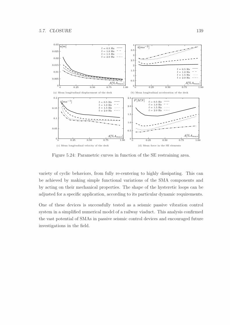
5.7. CLOSURE 139
f = 0.5 Hzf = 1.0 Hzf = 1.5 Hzf = 2.0 Hz
A[%Amax]
0.03
0.025
0.02
0.015
0.01
0.005
0
u[m]
1.000.750.500.250
1
f = 0.5 Hzf = 1.0 Hzf = 1.5 Hzf = 2.0 Hz
0.25 0.50 0.75 1.00
A[%Amax]
4
3.5
3
2.5
2
1.5
0.5
0
u[ms−2]
0
(a) Mean longitudinal displacement of the deck (b) Mean longitudinal acceleration of the deck
f = 0.5 Hzf = 1.0 Hzf = 1.5 Hzf = 2.0 Hz
A[%Amax]
0.2
0.15
0.1
0.05
00.25 0.50 0.75 1.00
u[ms−1]
0
f = 0.5 Hzf = 1.0 Hzf = 1.5 Hzf = 2.0 Hz
A[%Amax]
0.25 0.50 0.75 1.000
2.5
2.0
1.5
1.0
0.5
F [MN ]
0
(c) Mean longitudinal velocity of the deck (d) Mean force in the SE elements
Figure 5.24: Parametric curves in function of the SE restraining area.
variety of cyclic behaviors, from fully re-centering to highly dissipating. This can
be achieved by making simple functional variations of the SMA components and
by acting on their mechanical properties. The shape of the hysteretic loops can be
adjusted for a specific application, according to its particular dynamic requirements.
One of these devices is successfully tested as a seismic passive vibration control
system in a simplified numerical model of a railway viaduct. This analysis confirmed
the vast potential of SMAs in passive seismic control devices and encouraged future
investigations in the field.

140 CHAPTER 5. MODELING OF SE VIBRATION CONTROL DEVICES
Chapter 6
Novel Superelastic Device
6.1 Introduction
The proposed vibration control device derives from the SE passive dissipation device
proposed by Dolce et al. [52]. To increase its energy dissipation capabilities, the
original device is based on a set of pre-strained SE wires working in phase opposition.
However, a variety of stress-time effects observed in pre-strained SE wires [13] might
have an adverse impact on the dynamic performances of the device. Mainly to avoid
these problems, the proposed semi-active device uses a strategy that allows the
continuous adapting of the accumulated strain in the wires, based on the response
of the device to external excitations. As in an active control system, a controller
monitors the feedback measurements and generates appropriate command signals for
the device and, as in a passive control system, the control forces are developed as a
result of the motion of the structure itself, with no need of external energy input. As
the control forces act as to oppose the motion of the structural system, they promote
the global stability of the structure [73, 151, 153, 154, 156]. According to presently
accepted definitions the proposed device may be considered as a semi-active control
system.
141
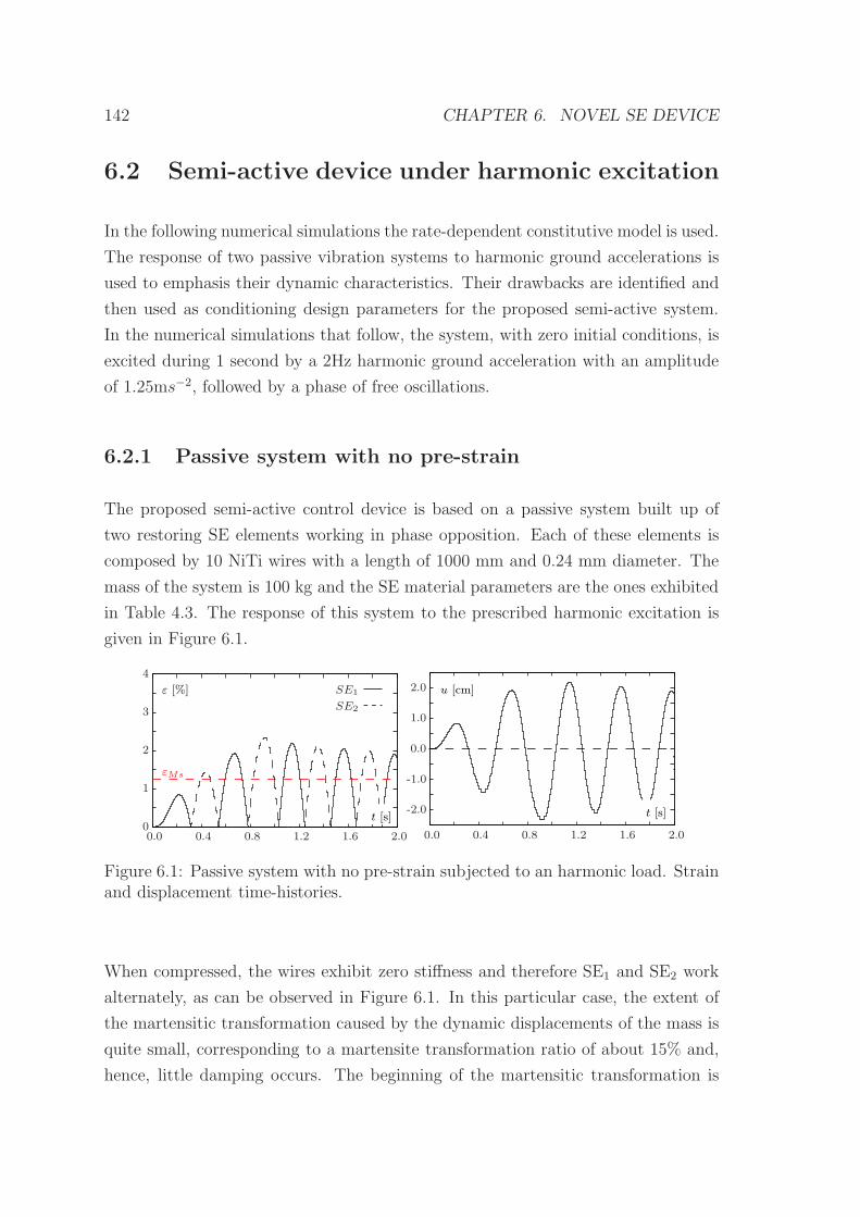
142 CHAPTER 6. NOVEL SE DEVICE
6.2 Semi-active device under harmonic excitation
In the following numerical simulations the rate-dependent constitutive model is used.
The response of two passive vibration systems to harmonic ground accelerations is
used to emphasis their dynamic characteristics. Their drawbacks are identified and
then used as conditioning design parameters for the proposed semi-active system.
In the numerical simulations that follow, the system, with zero initial conditions, is
excited during 1 second by a 2Hz harmonic ground acceleration with an amplitude
of 1.25ms−2, followed by a phase of free oscillations.
6.2.1 Passive system with no pre-strain
The proposed semi-active control device is based on a passive system built up of
two restoring SE elements working in phase opposition. Each of these elements is
composed by 10 NiTi wires with a length of 1000 mm and 0.24 mm diameter. The
mass of the system is 100 kg and the SE material parameters are the ones exhibited
in Table 4.3. The response of this system to the prescribed harmonic excitation is
given in Figure 6.1.
ε [%]
εMs
u [cm]2.0
1.0
-1.0
-2.0
0.0
3
2
1
0
4
0.0 0.4 0.8 1.2 1.6 2.00.0 0.4 0.8 1.2 1.6 2.0
t [s] t [s]
SE2
SE1
Figure 6.1: Passive system with no pre-strain subjected to an harmonic load. Strainand displacement time-histories.
When compressed, the wires exhibit zero stiffness and therefore SE1 and SE2 work
alternately, as can be observed in Figure 6.1. In this particular case, the extent of
the martensitic transformation caused by the dynamic displacements of the mass is
quite small, corresponding to a martensite transformation ratio of about 15% and,
hence, little damping occurs. The beginning of the martensitic transformation is
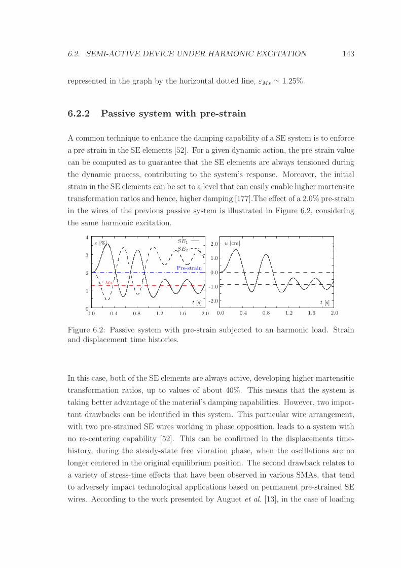
6.2. SEMI-ACTIVE DEVICE UNDER HARMONIC EXCITATION 143
represented in the graph by the horizontal dotted line, εMs ≃ 1.25%.
6.2.2 Passive system with pre-strain
A common technique to enhance the damping capability of a SE system is to enforce
a pre-strain in the SE elements [52]. For a given dynamic action, the pre-strain value
can be computed as to guarantee that the SE elements are always tensioned during
the dynamic process, contributing to the system’s response. Moreover, the initial
strain in the SE elements can be set to a level that can easily enable higher martensite
transformation ratios and hence, higher damping [177].The effect of a 2.0% pre-strain
in the wires of the previous passive system is illustrated in Figure 6.2, considering
the same harmonic excitation.
εMs
ε [%] u [cm]
Pre-strain
3
2
1
0
42.0
1.0
-1.0
-2.0
0.0
0.0 0.4 0.8 1.2 1.6 2.00.0 0.4 0.8 1.2 1.6 2.0
t [s]t [s]
SE2
SE1
Figure 6.2: Passive system with pre-strain subjected to an harmonic load. Strainand displacement time histories.
In this case, both of the SE elements are always active, developing higher martensitic
transformation ratios, up to values of about 40%. This means that the system is
taking better advantage of the material’s damping capabilities. However, two impor-
tant drawbacks can be identified in this system. This particular wire arrangement,
with two pre-strained SE wires working in phase opposition, leads to a system with
no re-centering capability [52]. This can be confirmed in the displacements time-
history, during the steady-state free vibration phase, when the oscillations are no
longer centered in the original equilibrium position. The second drawback relates to
a variety of stress-time effects that have been observed in various SMAs, that tend
to adversely impact technological applications based on permanent pre-strained SE
wires. According to the work presented by Auguet et al. [13], in the case of loading
144 CHAPTER 6. NOVEL SE DEVICE
under strain-controlled conditions, in the coexistence zone, stress seems to decrease
under constant strain. The fact that stress induced by pre-strain gradually dimin-
ishes with time is a limitation for seismic vibration control devices.
Another phenomenon that might hinder the use of pre-strained SE wires in passive
dissipation devices is the possible occurrence of permanent deformation due to cu-
mulative SMA creep [165]. When this happens, the length of the SE wire increases
continuously with cycling, meaning that, for a given oscillation amplitude, the strain
is reduced, along with the amount of dissipated mechanical energy.
Cumulative creep in Nitinol is linked with the introduction of dislocations and other
lattice defects generated at high stress, during the preceding loading cycle [107, 111].
Hence, this accumulated deformation may be controlled by keeping the SE wire in-
side certain recoverable limits in the SE window. These limits, which ensure an
appropriate material behavior, are determined by the material composition and its
thermo-mechanical treatment. In fact, the stability of the deformation behavior may
be improved by raising the critical stress for slip. Thermo-mechanical heat treat-
ments aimed to stabilize the SE behavior of Nitinol have been found effective [107],
minimizing cumulative creep and avoiding the modification of the hysteretic cycle.
While a simple solution, involving a third elastic element, exists in order to recover
the re-centering capability of the system [52, 53], the remaining problems related to
aging under stress and cumulative creep do not have a simple solution in a passive
device configuration. Aging under stress is difficult to avoid, as the use of permanent
pre-strained SE wires is crucial in order to obtain competitive damping ratios in
this type of systems. In what concerns the cumulative creep, keeping the strains
inside the SE window is a very challenging task when dealing with arbitrary seismic
excitation.
6.2.3 Semi-active system
The proposed semi-active control device minimizes the SMA rheological effects by
controlling the strain in the SE wires. The strain is self-adjusting, allowing the
wires to become strain/stress free, when not subjected to a dynamic excitation.
The system is also able to keep the wires deformation inside a given SE window,
while guaranteeing a minimal threshold to their strain level. The strain in the SE
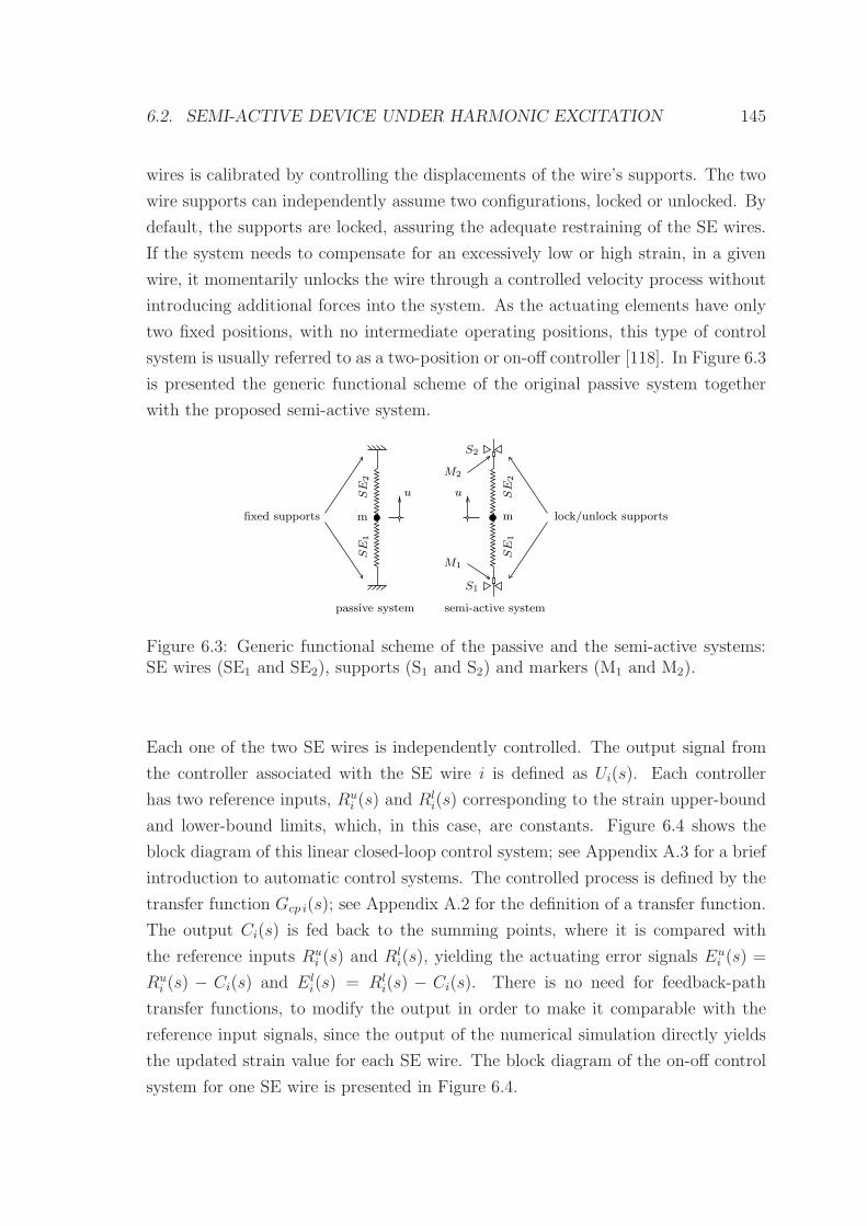
6.2. SEMI-ACTIVE DEVICE UNDER HARMONIC EXCITATION 145
wires is calibrated by controlling the displacements of the wire’s supports. The two
wire supports can independently assume two configurations, locked or unlocked. By
default, the supports are locked, assuring the adequate restraining of the SE wires.
If the system needs to compensate for an excessively low or high strain, in a given
wire, it momentarily unlocks the wire through a controlled velocity process without
introducing additional forces into the system. As the actuating elements have only
two fixed positions, with no intermediate operating positions, this type of control
system is usually referred to as a two-position or on-off controller [118]. In Figure 6.3
is presented the generic functional scheme of the original passive system together
with the proposed semi-active system.
lock/unlock supportsfixed supports
uu
M1
passive system semi-active system
M2
S1
S2
SE
1SE
2
mSE
1SE
2m
Figure 6.3: Generic functional scheme of the passive and the semi-active systems:SE wires (SE1 and SE2), supports (S1 and S2) and markers (M1 and M2).
Each one of the two SE wires is independently controlled. The output signal from
the controller associated with the SE wire i is defined as Ui(s). Each controller
has two reference inputs, Rui (s) and R
li(s) corresponding to the strain upper-bound
and lower-bound limits, which, in this case, are constants. Figure 6.4 shows the
block diagram of this linear closed-loop control system; see Appendix A.3 for a brief
introduction to automatic control systems. The controlled process is defined by the
transfer function Gcp i(s); see Appendix A.2 for the definition of a transfer function.
The output Ci(s) is fed back to the summing points, where it is compared with
the reference inputs Rui (s) and R
li(s), yielding the actuating error signals Eu
i (s) =
Rui (s) − Ci(s) and El
i(s) = Rli(s) − Ci(s). There is no need for feedback-path
transfer functions, to modify the output in order to make it comparable with the
reference input signals, since the output of the numerical simulation directly yields
the updated strain value for each SE wire. The block diagram of the on-off control
system for one SE wire is presented in Figure 6.4.
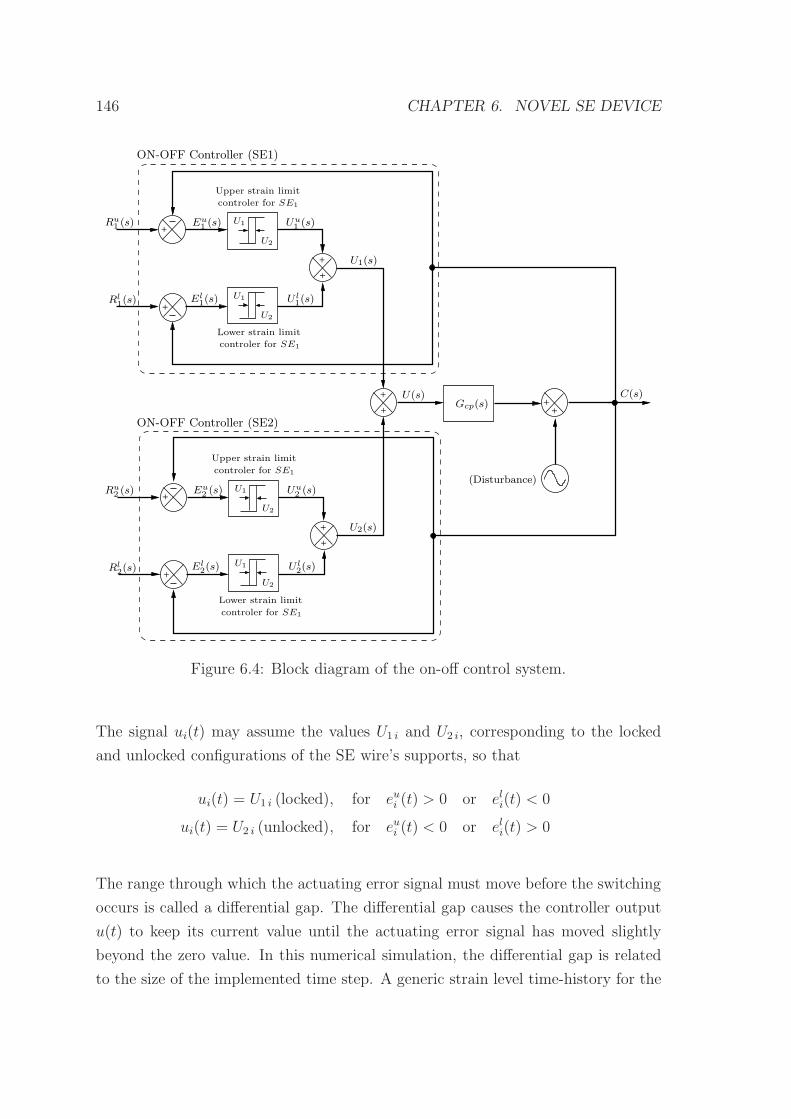
146 CHAPTER 6. NOVEL SE DEVICE
+
+
+
+
+
+
++
+
+
+
+
U1
U1
Gcp(s)
Upper strain limit
controler for SE1
Lower strain limit
controler for SE1
Upper strain limit
controler for SE1
Lower strain limit
controler for SE1
Ru1 (s)
Rl1(s)
Ru2 (s)
Rl2(s)
U2
U2
U1
U2
U2
U1
U(s)
El1(s) U l
1(s)
U1(s)
U2(s)
El2(s) U l
2(s)
Eu1 (s) Uu
1 (s)
Eu2 (s) Uu
2 (s)
ON-OFF Controller (SE1)
ON-OFF Controller (SE2)
(Disturbance)
C(s)
Figure 6.4: Block diagram of the on-off control system.
The signal ui(t) may assume the values U1 i and U2 i, corresponding to the locked
and unlocked configurations of the SE wire’s supports, so that
ui(t) = U1 i (locked), for eui (t) > 0 or eli(t) < 0
ui(t) = U2 i (unlocked), for eui (t) < 0 or eli(t) > 0
The range through which the actuating error signal must move before the switching
occurs is called a differential gap. The differential gap causes the controller output
u(t) to keep its current value until the actuating error signal has moved slightly
beyond the zero value. In this numerical simulation, the differential gap is related
to the size of the implemented time step. A generic strain level time-history for the
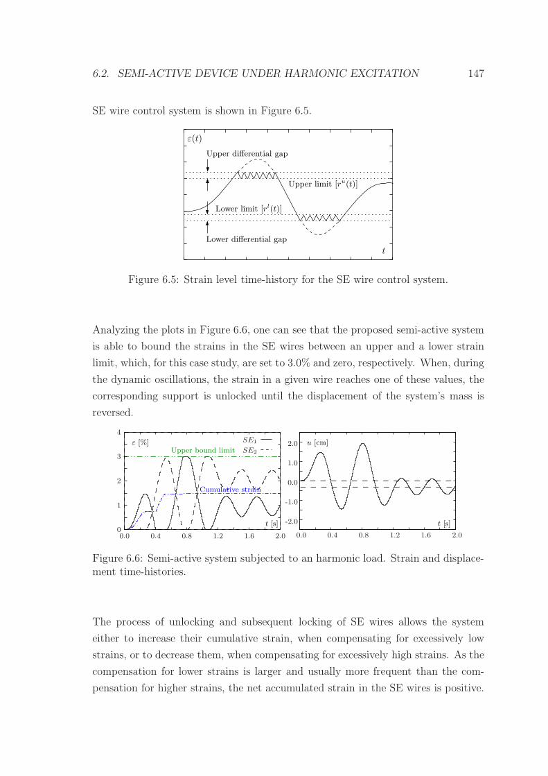
6.2. SEMI-ACTIVE DEVICE UNDER HARMONIC EXCITATION 147
SE wire control system is shown in Figure 6.5.
ε(t)
Upper differential gap
Lower differential gap
Upper limit [ru(t)]
Lower limit [rl(t)]
t
Figure 6.5: Strain level time-history for the SE wire control system.
Analyzing the plots in Figure 6.6, one can see that the proposed semi-active system
is able to bound the strains in the SE wires between an upper and a lower strain
limit, which, for this case study, are set to 3.0% and zero, respectively. When, during
the dynamic oscillations, the strain in a given wire reaches one of these values, the
corresponding support is unlocked until the displacement of the system’s mass is
reversed.
Cumulative strain
u [cm]ε [%]Upper bound limit
3
2
1
0
4
0.0 0.4 0.8 1.2 1.6 2.00.0 0.4 0.8 1.2 1.6 2.0
2.0
1.0
-1.0
-2.0
0.0
t [s] t [s]
SE2
SE1
Figure 6.6: Semi-active system subjected to an harmonic load. Strain and displace-ment time-histories.
The process of unlocking and subsequent locking of SE wires allows the system
either to increase their cumulative strain, when compensating for excessively low
strains, or to decrease them, when compensating for excessively high strains. As the
compensation for lower strains is larger and usually more frequent than the com-
pensation for higher strains, the net accumulated strain in the SE wires is positive.
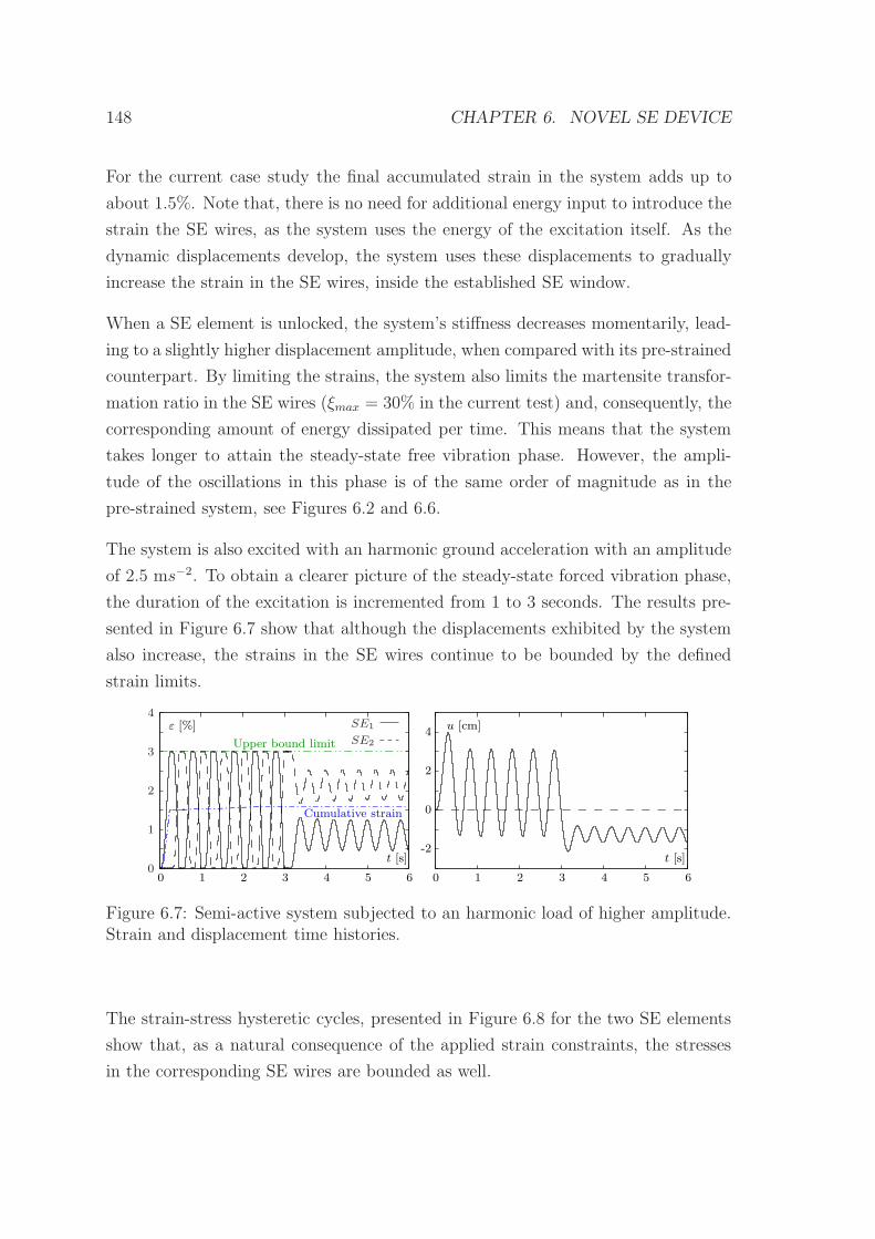
148 CHAPTER 6. NOVEL SE DEVICE
For the current case study the final accumulated strain in the system adds up to
about 1.5%. Note that, there is no need for additional energy input to introduce the
strain the SE wires, as the system uses the energy of the excitation itself. As the
dynamic displacements develop, the system uses these displacements to gradually
increase the strain in the SE wires, inside the established SE window.
When a SE element is unlocked, the system’s stiffness decreases momentarily, lead-
ing to a slightly higher displacement amplitude, when compared with its pre-strained
counterpart. By limiting the strains, the system also limits the martensite transfor-
mation ratio in the SE wires (ξmax = 30% in the current test) and, consequently, the
corresponding amount of energy dissipated per time. This means that the system
takes longer to attain the steady-state free vibration phase. However, the ampli-
tude of the oscillations in this phase is of the same order of magnitude as in the
pre-strained system, see Figures 6.2 and 6.6.
The system is also excited with an harmonic ground acceleration with an amplitude
of 2.5 ms−2. To obtain a clearer picture of the steady-state forced vibration phase,
the duration of the excitation is incremented from 1 to 3 seconds. The results pre-
sented in Figure 6.7 show that although the displacements exhibited by the system
also increase, the strains in the SE wires continue to be bounded by the defined
strain limits.
0 1 2 3 4 5 6 0 1 2 3 4 5 6
ε [%] u [cm]
Upper bound limit
Cumulative strain
4
2
0
-2t [s] t [s]
SE2
SE1
3
2
1
0
4
Figure 6.7: Semi-active system subjected to an harmonic load of higher amplitude.Strain and displacement time histories.
The strain-stress hysteretic cycles, presented in Figure 6.8 for the two SE elements
show that, as a natural consequence of the applied strain constraints, the stresses
in the corresponding SE wires are bounded as well.
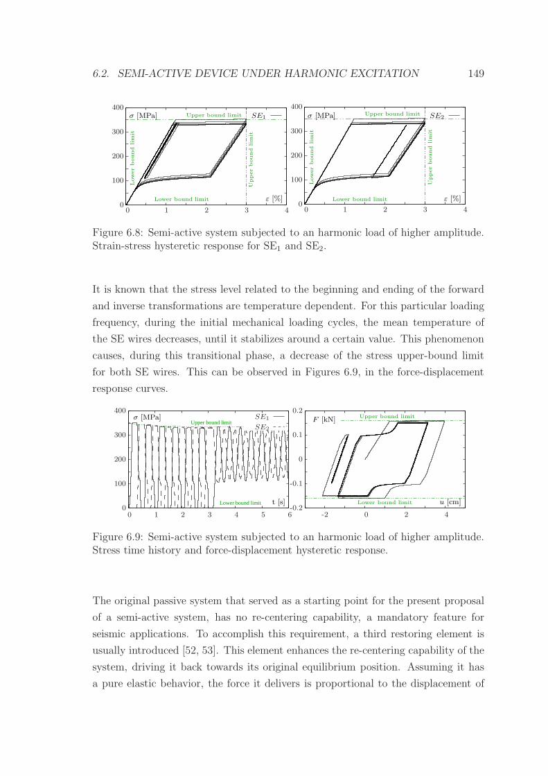
6.2. SEMI-ACTIVE DEVICE UNDER HARMONIC EXCITATION 149
SE2SE1σ [MPa]
ε [%]
σ [MPa]
ε [%]
Upperbound
lim
it
Upper bound limit
Lowerbound
lim
it
Lower bound limit
Lowerbound
lim
it
Upper bound limit
Lower bound limit
Upperbound
lim
it
3 4 0 21 3 40 1 20
100
200
300
400
100
200
300
400
0
Figure 6.8: Semi-active system subjected to an harmonic load of higher amplitude.Strain-stress hysteretic response for SE1 and SE2.
It is known that the stress level related to the beginning and ending of the forward
and inverse transformations are temperature dependent. For this particular loading
frequency, during the initial mechanical loading cycles, the mean temperature of
the SE wires decreases, until it stabilizes around a certain value. This phenomenon
causes, during this transitional phase, a decrease of the stress upper-bound limit
for both SE wires. This can be observed in Figures 6.9, in the force-displacement
response curves.
Upper bound limit
Lower bound limit
F [kN] Upper bound limit
Lower bound limit u [cm]
σ [MPa]
t [s]
1 2 3 4 5 6 -2 0 2 40
100
200
300
400
0 -0.2
-0.1
0
0.1
0.2
SE2
SE1
Figure 6.9: Semi-active system subjected to an harmonic load of higher amplitude.Stress time history and force-displacement hysteretic response.
The original passive system that served as a starting point for the present proposal
of a semi-active system, has no re-centering capability, a mandatory feature for
seismic applications. To accomplish this requirement, a third restoring element is
usually introduced [52, 53]. This element enhances the re-centering capability of the
system, driving it back towards its original equilibrium position. Assuming it has
a pure elastic behavior, the force it delivers is proportional to the displacement of
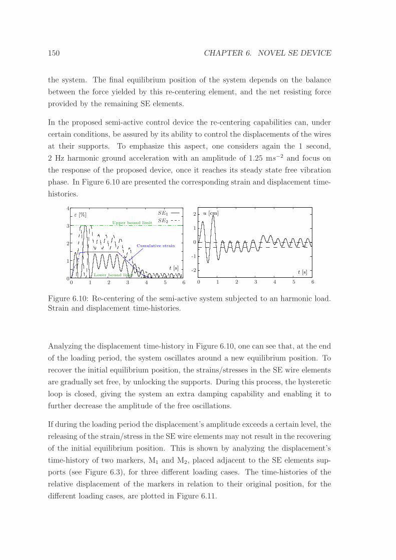
150 CHAPTER 6. NOVEL SE DEVICE
the system. The final equilibrium position of the system depends on the balance
between the force yielded by this re-centering element, and the net resisting force
provided by the remaining SE elements.
In the proposed semi-active control device the re-centering capabilities can, under
certain conditions, be assured by its ability to control the displacements of the wires
at their supports. To emphasize this aspect, one considers again the 1 second,
2 Hz harmonic ground acceleration with an amplitude of 1.25 ms−2 and focus on
the response of the proposed device, once it reaches its steady state free vibration
phase. In Figure 6.10 are presented the corresponding strain and displacement time-
histories.
Upper bound limit
Lower bound limit
ε [%] u [cm]
Cumulative strain
SE2
SE1
0 61 2 3 54 0 61 2 3 4 5
4
3
2
1
0
0
2
1
-1
-2t [s]t [s]
Figure 6.10: Re-centering of the semi-active system subjected to an harmonic load.Strain and displacement time-histories.
Analyzing the displacement time-history in Figure 6.10, one can see that, at the end
of the loading period, the system oscillates around a new equilibrium position. To
recover the initial equilibrium position, the strains/stresses in the SE wire elements
are gradually set free, by unlocking the supports. During this process, the hysteretic
loop is closed, giving the system an extra damping capability and enabling it to
further decrease the amplitude of the free oscillations.
If during the loading period the displacement’s amplitude exceeds a certain level, the
releasing of the strain/stress in the SE wire elements may not result in the recovering
of the initial equilibrium position. This is shown by analyzing the displacement’s
time-history of two markers, M1 and M2, placed adjacent to the SE elements sup-
ports (see Figure 6.3), for three different loading cases. The time-histories of the
relative displacement of the markers in relation to their original position, for the
different loading cases, are plotted in Figure 6.11.
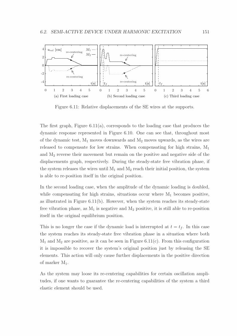
6.2. SEMI-ACTIVE DEVICE UNDER HARMONIC EXCITATION 151
t[s] t[s]t[s]
urel [cm]
(a) First loading case (b) Second loading case (c) Third loading case
tf tf-4
-2
0
2
4
M2
M1
0 1 2 3 4 5 60 1 2 3 4 50 1 2 3 4 5
re-centering
re-centering
re-centering
re-centering
Figure 6.11: Relative displacements of the SE wires at the supports.
The first graph, Figure 6.11(a), corresponds to the loading case that produces the
dynamic response represented in Figure 6.10. One can see that, throughout most
of the dynamic test, M1 moves downwards and M2 moves upwards, as the wires are
released to compensate for low strains. When compensating for high strains, M1
and M2 reverse their movement but remain on the positive and negative side of the
displacements graph, respectively. During the steady-state free vibration phase, if
the system releases the wires until M1 and M2 reach their initial position, the system
is able to re-position itself in the original position.
In the second loading case, when the amplitude of the dynamic loading is doubled,
while compensating for high strains, situations occur where M1 becomes positive,
as illustrated in Figure 6.11(b). However, when the system reaches its steady-state
free vibration phase, as M1 is negative and M2 positive, it is still able to re-position
itself in the original equilibrium position.
This is no longer the case if the dynamic load is interrupted at t = tf . In this case
the system reaches its steady-state free vibration phase in a situation where both
M1 and M2 are positive, as it can be seen in Figure 6.11(c). From this configuration
it is impossible to recover the system’s original position just by releasing the SE
elements. This action will only cause further displacements in the positive direction
of marker M1.
As the system may loose its re-centering capabilities for certain oscillation ampli-
tudes, if one wants to guarantee the re-centering capabilities of the system a third
elastic element should be used.
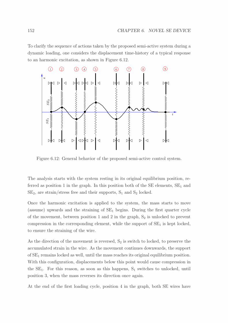
152 CHAPTER 6. NOVEL SE DEVICE
To clarify the sequence of actions taken by the proposed semi-active system during a
dynamic loading, one considers the displacement time-history of a typical response
to an harmonic excitation, as shown in Figure 6.12.
1 2 3 4 5 6 87 9
t
u
SE
2SE
1
Figure 6.12: General behavior of the proposed semi-active control system.
The analysis starts with the system resting in its original equilibrium position, re-
ferred as position 1 in the graph. In this position both of the SE elements, SE1 and
SE2, are strain/stress free and their supports, S1 and S2 locked.
Once the harmonic excitation is applied to the system, the mass starts to move
(assume) upwards and the straining of SE1 begins. During the first quarter cycle
of the movement, between position 1 and 2 in the graph, S2 is unlocked to prevent
compression in the corresponding element, while the support of SE1 is kept locked,
to ensure the straining of the wire.
As the direction of the movement is reversed, S2 is switch to locked, to preserve the
accumulated strain in the wire. As the movement continues downwards, the support
of SE1 remains locked as well, until the mass reaches its original equilibrium position.
With this configuration, displacements below this point would cause compression in
the SE1. For this reason, as soon as this happens, S1 switches to unlocked, until
position 3, when the mass reverses its direction once again.
At the end of the first loading cycle, position 4 in the graph, both SE wires have
6.3. SEMI-ACTIVE DEVICE UNDER SEISMIC EXCITATION 153
already accumulated a certain level of strain. Note that this strain was introduced
in the system by the external dynamic load itself, without any need of supplemental
energy input.
Between positions 4 and 5, assuming that in the last one occurs the maximum
displacement amplitude, both supports will switch from locked to unlocked: S2, as
the strain in SE2 approaches zero to avoid compression, and S1, as the strain in
SE1 goes beyond the defined value inside the SE window, preventing it from further
straining. If, during an eventual steady-state forced vibration phase, positions 5
to 6, there is no need for adjustments in the SE wires to compensate low or high
strains, both supports remain locked.
As soon as the dynamic excitation ceases, position 7, the amplitude of the free
vibrations starts gradually to diminish because of the SE damping. The system
reaches its steady-state free vibration phase, position 8, oscillating around an equi-
librium position different from its original one. During this period, both supports
remain locked. At this point, to recover the original equilibrium position, the system
unlocks both of the cables, relinquishing the accumulated strain in the wires.
Note that, every time the system needs to unlock a support, the wire is released
with a controlled velocity, which can be seen as a design parameter of the proposed
semi-active device. In all the reported numeric tests, this velocity is set to 0.6 m/s.
Finally, position 9, the supports are locked again to prepare the device for the next
dynamic excitation.
6.3 Semi-active device under seismic excitation
The efficiency of SE based passive control devices in the context of seismic loading
was already analyzed, considering a simplified numerical model of the Sao Martinho
railway viaduct. In this section, the same model is used to test the behavior of the
proposed semi-active control device under seismic excitation. For the longitudinal
analysis of the viaduct, it is assimilated to an elastic, SDOF dynamic system, with
4650 ton mass and a stiffness of 355×103 kN/m. An additional structural damping
of 5% is provided to the system in order to make the analysis more realistic.
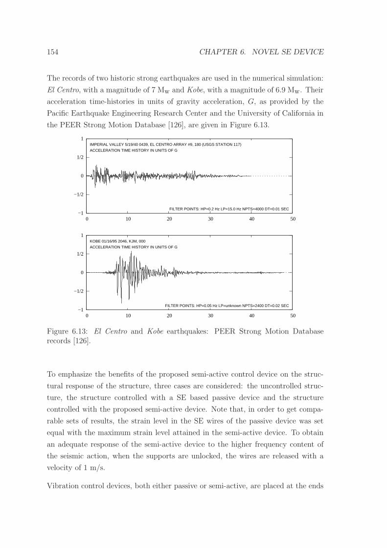
154 CHAPTER 6. NOVEL SE DEVICE
The records of two historic strong earthquakes are used in the numerical simulation:
El Centro, with a magnitude of 7 Mw and Kobe, with a magnitude of 6.9 Mw. Their
acceleration time-histories in units of gravity acceleration, G, as provided by the
Pacific Earthquake Engineering Research Center and the University of California in
the PEER Strong Motion Database [126], are given in Figure 6.13.
IMPERIAL VALLEY 5/19/40 0439, EL CENTRO ARRAY #9, 180 (USGS STATION 117)
ACCELERATION TIME HISTORY IN UNITS OF G
FILTER POINTS: HP=0.2 Hz LP=15.0 Hz NPTS=4000 DT=0.01 SEC
KOBE 01/16/95 2046, KJM, 000
ACCELERATION TIME HISTORY IN UNITS OF G
FILTER POINTS: HP=0.05 Hz LP=unknown NPTS=2400 DT=0.02 SEC
0 10 20 30 40 50−1
−1/2
0
1/2
1
0 10 20 30 40 50−1
−1/2
0
1/2
1
Figure 6.13: El Centro and Kobe earthquakes: PEER Strong Motion Databaserecords [126].
To emphasize the benefits of the proposed semi-active control device on the struc-
tural response of the structure, three cases are considered: the uncontrolled struc-
ture, the structure controlled with a SE based passive device and the structure
controlled with the proposed semi-active device. Note that, in order to get compa-
rable sets of results, the strain level in the SE wires of the passive device was set
equal with the maximum strain level attained in the semi-active device. To obtain
an adequate response of the semi-active device to the higher frequency content of
the seismic action, when the supports are unlocked, the wires are released with a
velocity of 1 m/s.
Vibration control devices, both either passive or semi-active, are placed at the ends
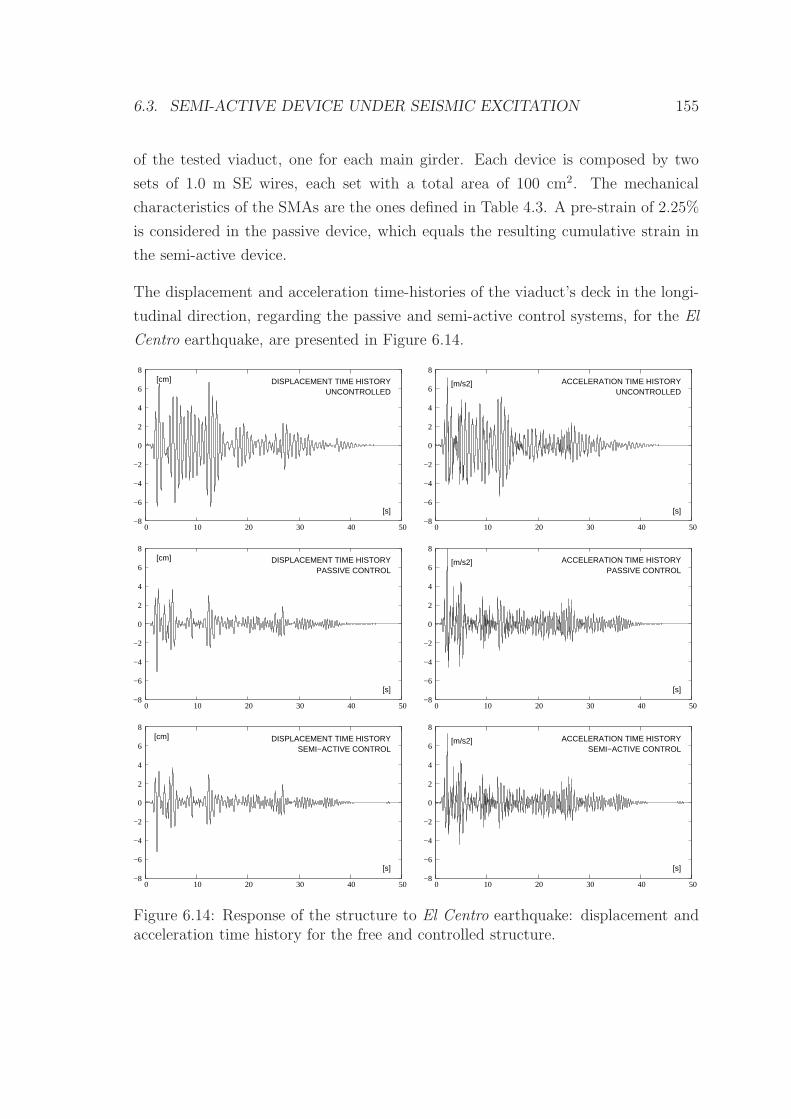
6.3. SEMI-ACTIVE DEVICE UNDER SEISMIC EXCITATION 155
of the tested viaduct, one for each main girder. Each device is composed by two
sets of 1.0 m SE wires, each set with a total area of 100 cm2. The mechanical
characteristics of the SMAs are the ones defined in Table 4.3. A pre-strain of 2.25%
is considered in the passive device, which equals the resulting cumulative strain in
the semi-active device.
The displacement and acceleration time-histories of the viaduct’s deck in the longi-
tudinal direction, regarding the passive and semi-active control systems, for the El
Centro earthquake, are presented in Figure 6.14.
DISPLACEMENT TIME HISTORYUNCONTROLLED
DISPLACEMENT TIME HISTORYPASSIVE CONTROL
DISPLACEMENT TIME HISTORYSEMI−ACTIVE CONTROL
ACCELERATION TIME HISTORYUNCONTROLLED
ACCELERATION TIME HISTORYPASSIVE CONTROL
ACCELERATION TIME HISTORYSEMI−ACTIVE CONTROL
[s]
[s][s]
[s][s]
[s]
[cm] [m/s2]
[m/s2]
[m/s2]
[cm]
[cm]
−8
−6
−4
−2
0
2
4
6
8
0 10 20 30 40 50
−8
−6
−4
−2
0
2
4
6
8
0 10 20 30 40 50
−8
−6
−4
−2
0
2
4
6
8
0 10 20 30 40 50
−8
−6
−4
−2
0
2
4
6
8
0 10 20 30 40 50
−8
−6
−4
−2
0
2
4
6
8
0 10 20 30 40 50
−8
−6
−4
−2
0
2
4
6
8
0 10 20 30 40 50
Figure 6.14: Response of the structure to El Centro earthquake: displacement andacceleration time history for the free and controlled structure.
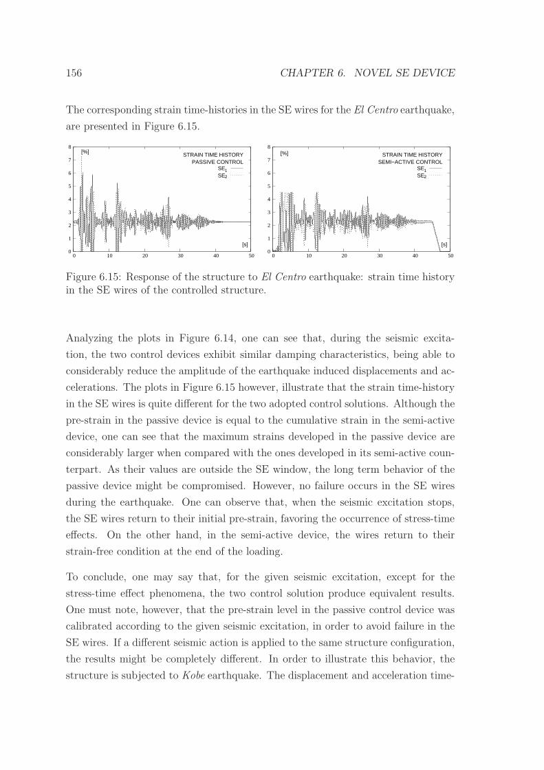
156 CHAPTER 6. NOVEL SE DEVICE
The corresponding strain time-histories in the SE wires for the El Centro earthquake,
are presented in Figure 6.15.
STRAIN TIME HISTORYPASSIVE CONTROL
21
[%]
[s]
STRAIN TIME HISTORYSEMI−ACTIVE CONTROL
21
[%]
[s]
SE SE
0
1
2
3
4
5
6
7
8
0 10 20 30 40 50 0
1
2
3
4
5
6
7
8
0 10 20 30 40 50
SE SE
Figure 6.15: Response of the structure to El Centro earthquake: strain time historyin the SE wires of the controlled structure.
Analyzing the plots in Figure 6.14, one can see that, during the seismic excita-
tion, the two control devices exhibit similar damping characteristics, being able to
considerably reduce the amplitude of the earthquake induced displacements and ac-
celerations. The plots in Figure 6.15 however, illustrate that the strain time-history
in the SE wires is quite different for the two adopted control solutions. Although the
pre-strain in the passive device is equal to the cumulative strain in the semi-active
device, one can see that the maximum strains developed in the passive device are
considerably larger when compared with the ones developed in its semi-active coun-
terpart. As their values are outside the SE window, the long term behavior of the
passive device might be compromised. However, no failure occurs in the SE wires
during the earthquake. One can observe that, when the seismic excitation stops,
the SE wires return to their initial pre-strain, favoring the occurrence of stress-time
effects. On the other hand, in the semi-active device, the wires return to their
strain-free condition at the end of the loading.
To conclude, one may say that, for the given seismic excitation, except for the
stress-time effect phenomena, the two control solution produce equivalent results.
One must note, however, that the pre-strain level in the passive control device was
calibrated according to the given seismic excitation, in order to avoid failure in the
SE wires. If a different seismic action is applied to the same structure configuration,
the results might be completely different. In order to illustrate this behavior, the
structure is subjected to Kobe earthquake. The displacement and acceleration time-
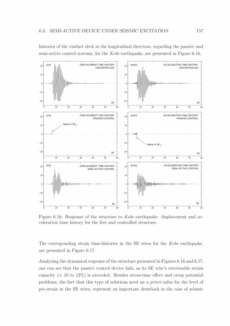
6.3. SEMI-ACTIVE DEVICE UNDER SEISMIC EXCITATION 157
histories of the viaduct deck in the longitudinal direction, regarding the passive and
semi-active control systems, for the Kobe earthquake, are presented in Figure 6.16.
2
DISPLACEMENT TIME HISTORYPASSIVE CONTROL
DISPLACEMENT TIME HISTORYUNCONTROLLED
DISPLACEMENT TIME HISTORYSEMI−ACTIVE CONTROL
ACCELERATION TIME HISTORYUNCONTROLLED
ACCELERATION TIME HISTORYSEMI−ACTIVE CONTROL
2
[s]
[s]
[s] [s]
[s]
[s]
[m/s2]
[m/s2]
[m/s2][cm]
[cm]
[cm]
ACCELERATION TIME HISTORYPASSIVE CONTROL
failure in SE
−20
−10
0
10
20
0 10 20 30 40 50 60
−20
−10
0
10
20
0 10 20 30 40 50 60
−20
−10
0
10
20
0 10 20 30 40 50 60
−20
−10
0
10
20
0 10 20 30 40 50 60
failure in SE
−20
−10
−20
−10
0
10
20
0 10 20 30 40 50 60
0
10
20
0 10 20 30 40 50 60
Figure 6.16: Response of the structure to Kobe earthquake: displacement and ac-celeration time history for the free and controlled structure.
The corresponding strain time-histories in the SE wires for the Kobe earthquake,
are presented in Figure 6.17.
Analyzing the dynamical response of the structure presented in Figures 6.16 and 6.17,
one can see that the passive control device fails, as its SE wire’s recoverable strain
capacity (≃ 10 to 12%) is exceeded. Besides stress-time effect and creep potential
problems, the fact that this type of solutions need an a priori value for the level of
pre-strain in the SE wires, represent an important drawback in the case of seismic
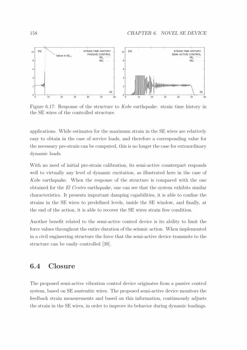
158 CHAPTER 6. NOVEL SE DEVICE
STRAIN TIME HISTORYSEMI−ACTIVE CONTROL
21
STRAIN TIME HISTORYPASSIVE CONTROL
21
[%]
[s][s]
[%]
2
0
2
4
6
8
10
0 10 20 30 40 50 60
SE SE
SE SE
0
2
4
6
8
10
0 10 20 30 40 50 60
failure in SE
Figure 6.17: Response of the structure to Kobe earthquake: strain time history inthe SE wires of the controlled structure.
applications. While estimates for the maximum strain in the SE wires are relatively
easy to obtain in the case of service loads, and therefore a corresponding value for
the necessary pre-strain can be computed, this is no longer the case for extraordinary
dynamic loads.
With no need of initial pre-strain calibration, its semi-active counterpart responds
well to virtually any level of dynamic excitation, as illustrated here in the case of
Kobe earthquake. When the response of the structure is compared with the one
obtained for the El Centro earthquake, one can see that the system exhibits similar
characteristics. It presents important damping capabilities, it is able to confine the
strains in the SE wires to predefined levels, inside the SE window, and finally, at
the end of the action, it is able to recover the SE wires strain free condition.
Another benefit related to the semi-active control device is its ability to limit the
force values throughout the entire duration of the seismic action. When implemented
in a civil engineering structure the force that the semi-active device transmits to the
structure can be easily controlled [39].
6.4 Closure
The proposed semi-active vibration control device originates from a passive control
system, based on SE austenitic wires. The proposed semi-active device monitors the
feedback strain measurements and based on this information, continuously adjusts
the strain in the SE wires, in order to improve its behavior during dynamic loadings.
6.4. CLOSURE 159
Permanent pre-strain in the SE wires is avoided since the strain accumulation results
from the structural displacements during a dynamic action, with no need for external
energy input. Stress-time effects in the SE wires are hence prevented. The SE wires
are also set strain free at the end of the loading period.
The system is able to dissipate a considerable amount of energy while keeping the SE
wires inside recoverable limits defined by a prescribed SE window, minimizing the
effects related to cumulative creep. The system also guarantees a minimal threshold
to the strain level in the SE wires and exhibits efficient re-centering capabilities.
The numerical simulations demonstrate the potential of the proposed semi-active
control device in improving the seismic response of civil engineering structures.

160 CHAPTER 6. NOVEL SE DEVICE
Chapter 7
Prototype of the Novel SE Device
7.1 Introduction
In this chapter is presented a prototype of the novel vibration control device de-
scribed in Chapter 6. The aim of this physical prototype is to further clarify and
substantiate the results obtained during the numeric simulations. The main idea
underlying the proposed semi-active control device is to improve the seismic behav-
ior of a SE bridge restraining system, by limiting the corresponding strains/stresses
inside a given SE window. Another important aspect of the proposed prototype is
that the SE elements are strain/stress free up to the moment the dynamic excitation
arises. With the beginning of the dynamic excitation the cumulative strain/stress
process in the SE wires starts, enabling higher martensite transformations ratios and
increased damping capacities in the system. The cumulative strain/stress in the SE
wires is a direct result of the system’s movement, which derives from the dynamic
excitation.
7.2 Building the prototype
The prototype simulates the behavior of a bridge with SE restrainer cables in the
deck-abutment interfaces, to limit the respective hinge opening during a dynamic
event. In Figure 7.5 is shown a schematic drawing of a simple supported bridge with
such a restraining system.
161
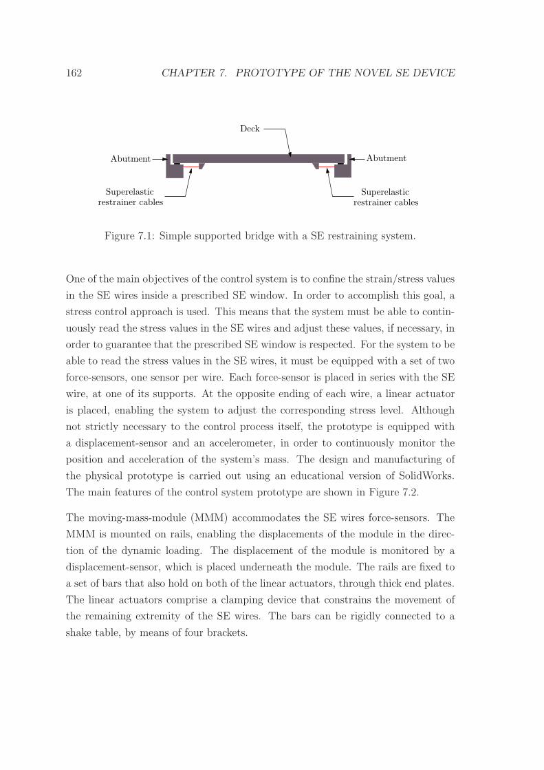
162 CHAPTER 7. PROTOTYPE OF THE NOVEL SE DEVICE
Superelasticrestrainer cables
Superelasticrestrainer cables
Abutment Abutment
Deck
Figure 7.1: Simple supported bridge with a SE restraining system.
One of the main objectives of the control system is to confine the strain/stress values
in the SE wires inside a prescribed SE window. In order to accomplish this goal, a
stress control approach is used. This means that the system must be able to contin-
uously read the stress values in the SE wires and adjust these values, if necessary, in
order to guarantee that the prescribed SE window is respected. For the system to be
able to read the stress values in the SE wires, it must be equipped with a set of two
force-sensors, one sensor per wire. Each force-sensor is placed in series with the SE
wire, at one of its supports. At the opposite ending of each wire, a linear actuator
is placed, enabling the system to adjust the corresponding stress level. Although
not strictly necessary to the control process itself, the prototype is equipped with
a displacement-sensor and an accelerometer, in order to continuously monitor the
position and acceleration of the system’s mass. The design and manufacturing of
the physical prototype is carried out using an educational version of SolidWorks.
The main features of the control system prototype are shown in Figure 7.2.
The moving-mass-module (MMM) accommodates the SE wires force-sensors. The
MMM is mounted on rails, enabling the displacements of the module in the direc-
tion of the dynamic loading. The displacement of the module is monitored by a
displacement-sensor, which is placed underneath the module. The rails are fixed to
a set of bars that also hold on both of the linear actuators, through thick end plates.
The linear actuators comprise a clamping device that constrains the movement of
the remaining extremity of the SE wires. The bars can be rigidly connected to a
shake table, by means of four brackets.

7.2. BUILDING THE PROTOTYPE 163
Linear actuator 1
Linear actuator 2
Moving mass module
Bar
RailClamp
End plate
Bracket
Figure 7.2: General design concept for the physical prototype.
7.2.1 Moving-mass-module
One of the kernel elements of the physical prototype is the MMM. The specifications
for the design of this component mainly derive from these requisites:
1. As the physical prototype represents a SDOF dynamic system, the movement
of the mass is limited to one direction. This movement has to be extremely
smooth, involving the least possible friction;
2. The value of the mass should be able to vary, as to increase the system’s
experimental redundancy;
3. The moving mass system has to integrate two force-sensors for the SE wires,
to continuously monitor their stress level;
4. The moving mass system has to comprehend a displacement-sensor in order
to monitor its displacement with respect to the shake-table;
5. The moving mass system has to comprehend an accelerometer in order to
monitor its acceleration.

164 CHAPTER 7. PROTOTYPE OF THE NOVEL SE DEVICE
In order to comply with these requisites, the MMM is built up as a modular system.
The base of the module is made of a CK45 steel plate, with dimensions a = 10,
b = 20 and c = 30 mm. This base presents five holes in order to make it lighter.
The base module accommodates a series of additional steel plates, with different
dimensions and weights, which are fixed to the base plate by two metallic pins.
The mass of the moving mass base, as well as of the additional mass modules are
presented in Table 7.2.
Element Mass (kg)
Base 0.545M1 0.497M2 0.980M3 2.035M4 2.043
Table 7.1: Mass of the MMM elements.
These pins constitute two rounded head cylinders, with a total length of 100 mm and
a diameter of 8 mm. The MMM is provided with a set of four steel beveled shape
wheels, with RHP 618/8 bearings and is mounted on a set of two 40×10×300 mm
AW-6063-T6 aluminum bars, with wedged shape rails. As the angle presented by the
wedge shaped rails is wider than the one shown by beveled wheels, the contact area
between the two pieces is minimized, reducing the mechanical friction developed in
this interface. In Figure 7.3 is presented the result of the design phase of the MMM,
including a general view of the module and a detail of the wheel-rail interface.
7.2.1.1 Force-sensors
In order to characterize the SE wires stress state, the MMM has to be provided
with a set of two force-sensors. Given the limited dimensions of the module, the
space available for the positioning of these sensors is quite reduced. Although one
can easily find several types of miniature load cells on the market, their price is
not compatible with the budget set for building the physical prototype. Hence, the
alternative option is to design and built the force-sensors, taking into consideration
the dimensional restrictions, the desired performance in terms of force readings and
also the limited budget. The idea underlying the behavior of the force-sensor is
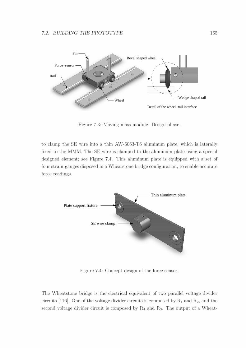
7.2. BUILDING THE PROTOTYPE 165
Pin
Rail
Detail of the wheel−rail interface
Wedge shaped rail
Bevel shaped wheel
Force−sensor
Wheel
Figure 7.3: Moving-mass-module. Design phase.
to clamp the SE wire into a thin AW-6063-T6 aluminum plate, which is laterally
fixed to the MMM. The SE wire is clamped to the aluminum plate using a special
designed element; see Figure 7.4. This aluminum plate is equipped with a set of
four strain-gauges disposed in a Wheatstone bridge configuration, to enable accurate
force readings.
Thin aluminum plate
SE wire clamp
Plate support fixture
Figure 7.4: Concept design of the force-sensor.
The Wheatstone bridge is the electrical equivalent of two parallel voltage divider
circuits [116]. One of the voltage divider circuits is composed by R1 and R2, and the
second voltage divider circuit is composed by R4 and R3. The output of a Wheat-
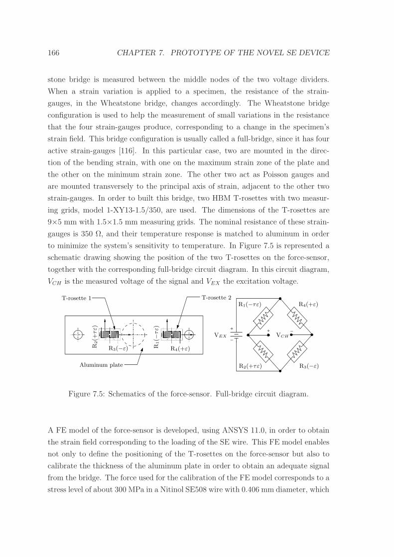
166 CHAPTER 7. PROTOTYPE OF THE NOVEL SE DEVICE
stone bridge is measured between the middle nodes of the two voltage dividers.
When a strain variation is applied to a specimen, the resistance of the strain-
gauges, in the Wheatstone bridge, changes accordingly. The Wheatstone bridge
configuration is used to help the measurement of small variations in the resistance
that the four strain-gauges produce, corresponding to a change in the specimen’s
strain field. This bridge configuration is usually called a full-bridge, since it has four
active strain-gauges [116]. In this particular case, two are mounted in the direc-
tion of the bending strain, with one on the maximum strain zone of the plate and
the other on the minimum strain zone. The other two act as Poisson gauges and
are mounted transversely to the principal axis of strain, adjacent to the other two
strain-gauges. In order to built this bridge, two HBM T-rosettes with two measur-
ing grids, model 1-XY13-1.5/350, are used. The dimensions of the T-rosettes are
9×5 mm with 1.5×1.5 mm measuring grids. The nominal resistance of these strain-
gauges is 350 Ω, and their temperature response is matched to aluminum in order
to minimize the system’s sensitivity to temperature. In Figure 7.5 is represented a
schematic drawing showing the position of the two T-rosettes on the force-sensor,
together with the corresponding full-bridge circuit diagram. In this circuit diagram,
VCH is the measured voltage of the signal and VEX the excitation voltage.
−
+ + −
T-rosette 1
Aluminum plate
T-rosette 2
R2(+τε)
R1(−τε)
VCHVEX
R4(+ε)
R3(−ε)
R4(+ε)R3(−ε)R2(+
τε)
R1(−
τε)
Figure 7.5: Schematics of the force-sensor. Full-bridge circuit diagram.
A FE model of the force-sensor is developed, using ANSYS 11.0, in order to obtain
the strain field corresponding to the loading of the SE wire. This FE model enables
not only to define the positioning of the T-rosettes on the force-sensor but also to
calibrate the thickness of the aluminum plate in order to obtain an adequate signal
from the bridge. The force used for the calibration of the FE model corresponds to a
stress level of about 300 MPa in a Nitinol SE508 wire with 0.406 mm diameter, which
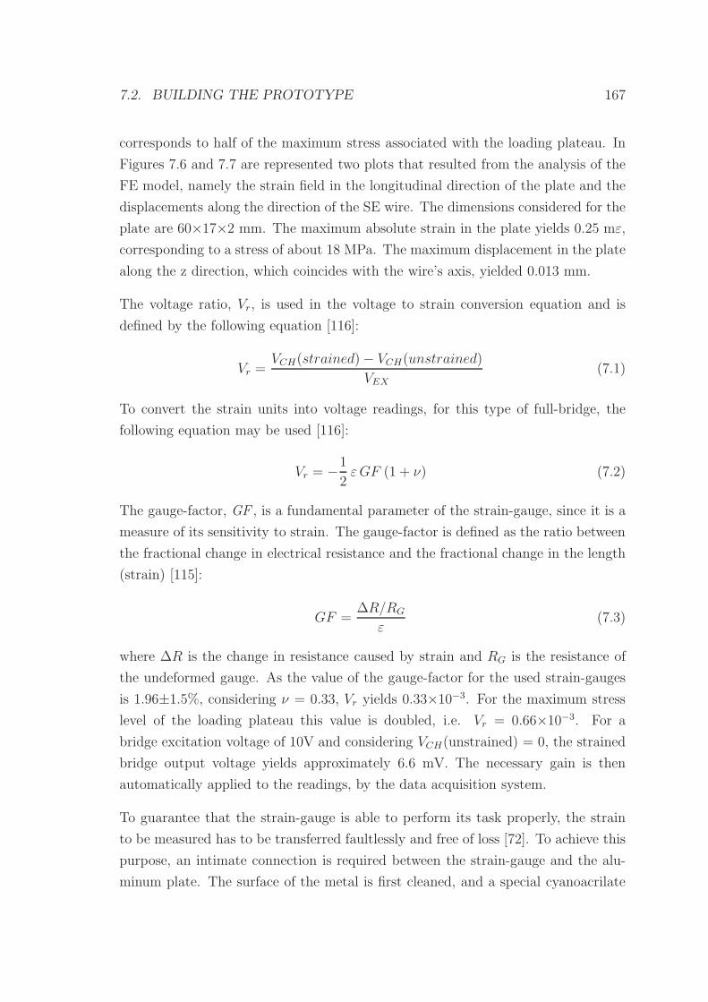
7.2. BUILDING THE PROTOTYPE 167
corresponds to half of the maximum stress associated with the loading plateau. In
Figures 7.6 and 7.7 are represented two plots that resulted from the analysis of the
FE model, namely the strain field in the longitudinal direction of the plate and the
displacements along the direction of the SE wire. The dimensions considered for the
plate are 60×17×2 mm. The maximum absolute strain in the plate yields 0.25 mε,
corresponding to a stress of about 18 MPa. The maximum displacement in the plate
along the z direction, which coincides with the wire’s axis, yielded 0.013 mm.
The voltage ratio, Vr, is used in the voltage to strain conversion equation and is
defined by the following equation [116]:
Vr =VCH(strained)− VCH(unstrained)
VEX(7.1)
To convert the strain units into voltage readings, for this type of full-bridge, the
following equation may be used [116]:
Vr = −1
2εGF (1 + ν) (7.2)
The gauge-factor, GF , is a fundamental parameter of the strain-gauge, since it is a
measure of its sensitivity to strain. The gauge-factor is defined as the ratio between
the fractional change in electrical resistance and the fractional change in the length
(strain) [115]:
GF =∆R/RG
ε(7.3)
where ∆R is the change in resistance caused by strain and RG is the resistance of
the undeformed gauge. As the value of the gauge-factor for the used strain-gauges
is 1.96±1.5%, considering ν = 0.33, Vr yields 0.33×10⁻³. For the maximum stress
level of the loading plateau this value is doubled, i.e. Vr = 0.66×10⁻³. For a
bridge excitation voltage of 10V and considering VCH(unstrained) = 0, the strained
bridge output voltage yields approximately 6.6 mV. The necessary gain is then
automatically applied to the readings, by the data acquisition system.
To guarantee that the strain-gauge is able to perform its task properly, the strain
to be measured has to be transferred faultlessly and free of loss [72]. To achieve this
purpose, an intimate connection is required between the strain-gauge and the alu-
minum plate. The surface of the metal is first cleaned, and a special cyanoacrilate
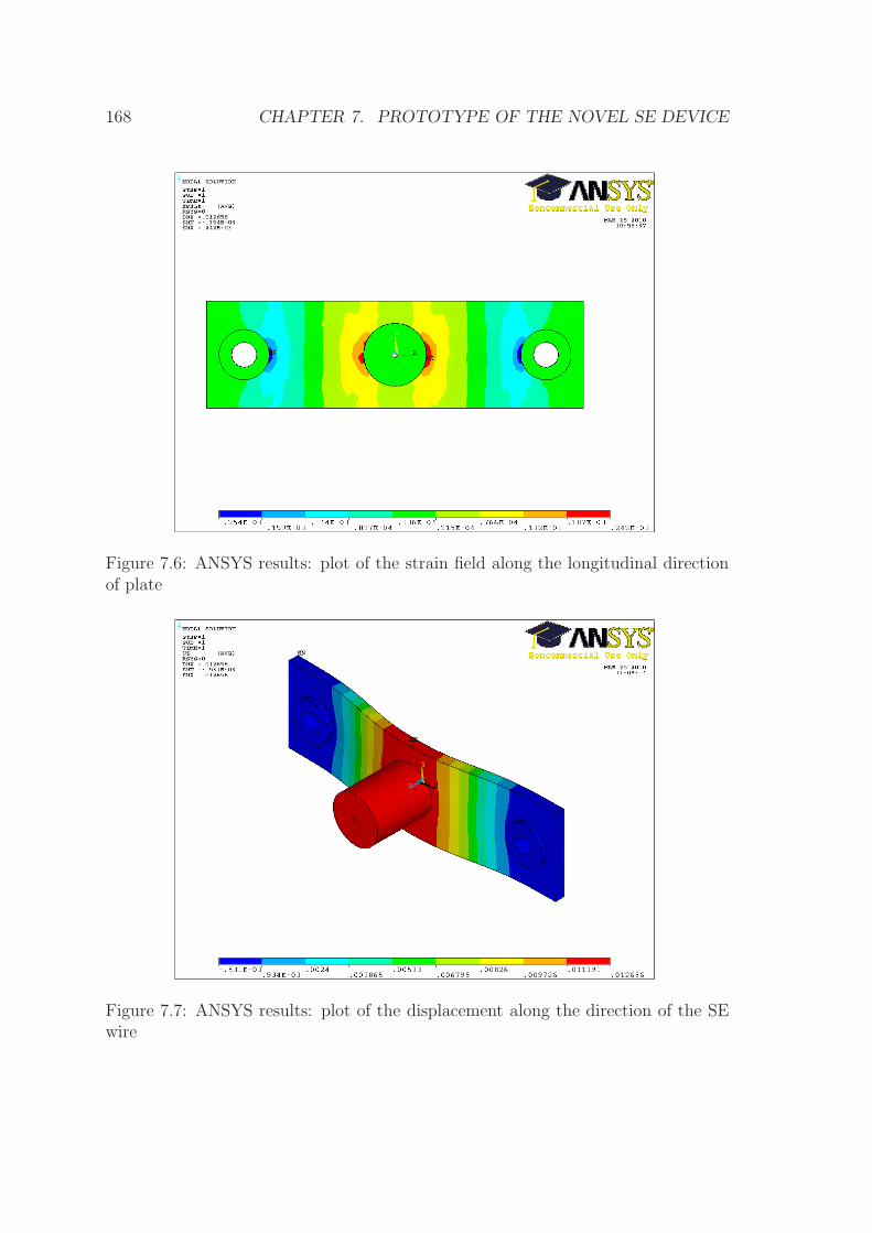
168 CHAPTER 7. PROTOTYPE OF THE NOVEL SE DEVICE
Figure 7.6: ANSYS results: plot of the strain field along the longitudinal directionof plate
Figure 7.7: ANSYS results: plot of the displacement along the direction of the SEwire
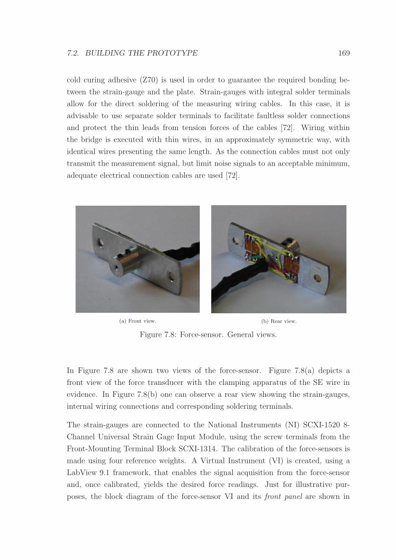
7.2. BUILDING THE PROTOTYPE 169
cold curing adhesive (Z70) is used in order to guarantee the required bonding be-
tween the strain-gauge and the plate. Strain-gauges with integral solder terminals
allow for the direct soldering of the measuring wiring cables. In this case, it is
advisable to use separate solder terminals to facilitate faultless solder connections
and protect the thin leads from tension forces of the cables [72]. Wiring within
the bridge is executed with thin wires, in an approximately symmetric way, with
identical wires presenting the same length. As the connection cables must not only
transmit the measurement signal, but limit noise signals to an acceptable minimum,
adequate electrical connection cables are used [72].
(a) Front view. (b) Rear view.
Figure 7.8: Force-sensor. General views.
In Figure 7.8 are shown two views of the force-sensor. Figure 7.8(a) depicts a
front view of the force transducer with the clamping apparatus of the SE wire in
evidence. In Figure 7.8(b) one can observe a rear view showing the strain-gauges,
internal wiring connections and corresponding soldering terminals.
The strain-gauges are connected to the National Instruments (NI) SCXI-1520 8-
Channel Universal Strain Gage Input Module, using the screw terminals from the
Front-Mounting Terminal Block SCXI-1314. The calibration of the force-sensors is
made using four reference weights. A Virtual Instrument (VI) is created, using a
LabView 9.1 framework, that enables the signal acquisition from the force-sensor
and, once calibrated, yields the desired force readings. Just for illustrative pur-
poses, the block diagram of the force-sensor VI and its front panel are shown in
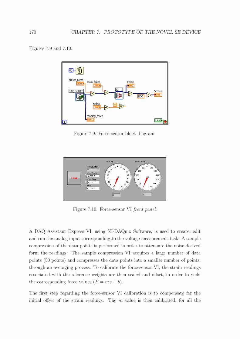
170 CHAPTER 7. PROTOTYPE OF THE NOVEL SE DEVICE
Figures 7.9 and 7.10.
Figure 7.9: Force-sensor block diagram.
Figure 7.10: Force-sensor VI front panel.
A DAQ Assistant Express VI, using NI-DAQmx Software, is used to create, edit
and run the analog input corresponding to the voltage measurement task. A sample
compression of the data points is performed in order to attenuate the noise derived
form the readings. The sample compression VI acquires a large number of data
points (50 points) and compresses the data points into a smaller number of points,
through an averaging process. To calibrate the force-sensor VI, the strain readings
associated with the reference weights are then scaled and offset, in order to yield
the corresponding force values (F = mε+ b).
The first step regarding the force-sensor VI calibration is to compensate for the
initial offset of the strain readings. The m value is then calibrated, for all the
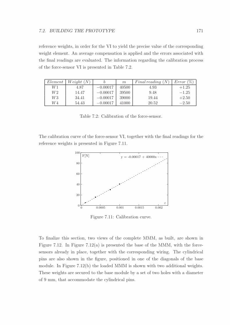
7.2. BUILDING THE PROTOTYPE 171
reference weights, in order for the VI to yield the precise value of the corresponding
weight element. An average compensation is applied and the errors associated with
the final readings are evaluated. The information regarding the calibration process
of the force-sensor VI is presented in Table 7.2.
Element Weight (N) b m Final reading (N) Error (%)
W1 4.87 −0.00017 40500 4.93 +1.25W2 14.47 −0.00017 39500 9.48 −1.25W3 34.41 −0.00017 39000 19.44 +2.50W4 54.43 −0.00017 41000 20.52 −2.50
Table 7.2: Calibration of the force-sensor.
The calibration curve of the force-sensor VI, together with the final readings for the
reference weights is presented in Figure 7.11.
80
100
60
40
20
00 0.0005 0.001 0.0015 0.002
ε
y = -0.00017 + 40000xF[N]
Figure 7.11: Calibration curve.
To finalize this section, two views of the complete MMM, as built, are shown in
Figure 7.12. In Figure 7.12(a) is presented the base of the MMM, with the force-
sensors already in place, together with the corresponding wiring. The cylindrical
pins are also shown in the figure, positioned in one of the diagonals of the base
module. In Figure 7.12(b) the loaded MMM is shown with two additional weights.
These weights are secured to the base module by a set of two holes with a diameter
of 9 mm, that accommodate the cylindrical pins.
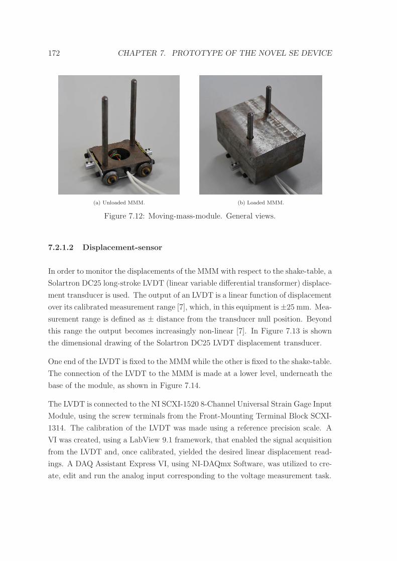
172 CHAPTER 7. PROTOTYPE OF THE NOVEL SE DEVICE
(a) Unloaded MMM. (b) Loaded MMM.
Figure 7.12: Moving-mass-module. General views.
7.2.1.2 Displacement-sensor
In order to monitor the displacements of the MMM with respect to the shake-table, a
Solartron DC25 long-stroke LVDT (linear variable differential transformer) displace-
ment transducer is used. The output of an LVDT is a linear function of displacement
over its calibrated measurement range [7], which, in this equipment is±25 mm. Mea-
surement range is defined as ± distance from the transducer null position. Beyond
this range the output becomes increasingly non-linear [7]. In Figure 7.13 is shown
the dimensional drawing of the Solartron DC25 LVDT displacement transducer.
One end of the LVDT is fixed to the MMM while the other is fixed to the shake-table.
The connection of the LVDT to the MMM is made at a lower level, underneath the
base of the module, as shown in Figure 7.14.
The LVDT is connected to the NI SCXI-1520 8-Channel Universal Strain Gage Input
Module, using the screw terminals from the Front-Mounting Terminal Block SCXI-
1314. The calibration of the LVDT was made using a reference precision scale. A
VI was created, using a LabView 9.1 framework, that enabled the signal acquisition
from the LVDT and, once calibrated, yielded the desired linear displacement read-
ings. A DAQ Assistant Express VI, using NI-DAQmx Software, was utilized to cre-
ate, edit and run the analog input corresponding to the voltage measurement task.
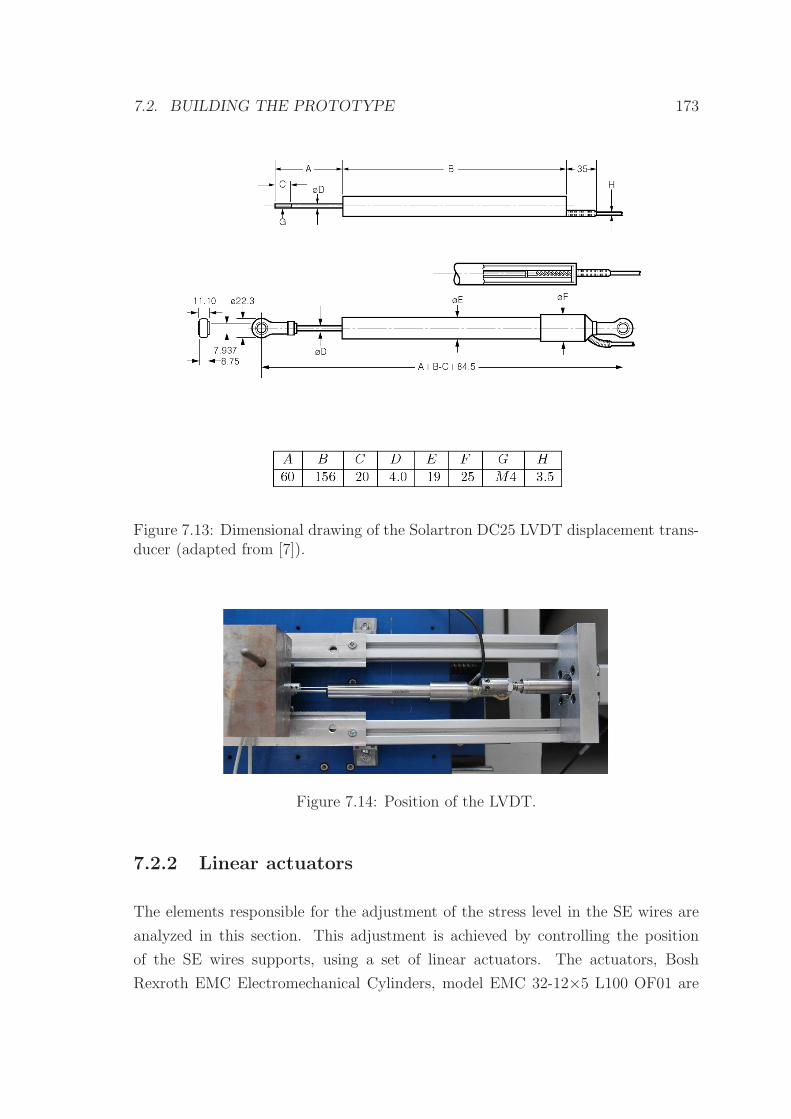
7.2. BUILDING THE PROTOTYPE 173
Figure 7.13: Dimensional drawing of the Solartron DC25 LVDT displacement trans-ducer (adapted from [7]).
Figure 7.14: Position of the LVDT.
7.2.2 Linear actuators
The elements responsible for the adjustment of the stress level in the SE wires are
analyzed in this section. This adjustment is achieved by controlling the position
of the SE wires supports, using a set of linear actuators. The actuators, Bosh
Rexroth EMC Electromechanical Cylinders, model EMC 32-12×5 L100 OF01 are
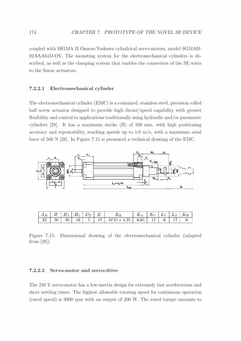
174 CHAPTER 7. PROTOTYPE OF THE NOVEL SE DEVICE
coupled with SIGMA II Omron-Yaskawa cylindrical servo-motors, model SGMAH-
02AAA61D-OY. The mounting system for the electromechanical cylinders is de-
scribed, as well as the clamping system that enables the connection of the SE wires
to the linear actuators.
7.2.2.1 Electromechanical cylinder
The electromechanical cylinder (EMC) is a contained, stainless steel, precision rolled
ball screw actuator designed to provide high thrust/speed capability with greater
flexibility and control to applications traditionally using hydraulic and/or pneumatic
cylinders [28]. It has a maximum stroke (H) of 100 mm, with high positioning
accuracy and repeatability, reaching speeds up to 1.6 m/s, with a maximum axial
force of 500 N [28]. In Figure 7.15 is presented a technical drawing of the EMC.
Figure 7.15: Dimensional drawing of the electromechanical cylinder (adaptedfrom [28]).
7.2.2.2 Servo-motor and servo-drive
The 230 V servo-motor has a low-inertia design for extremely fast accelerations and
short settling times. The highest allowable rotating speed for continuous operation
(rated speed) is 3000 rpm with an output of 200 W. The rated torque amounts to
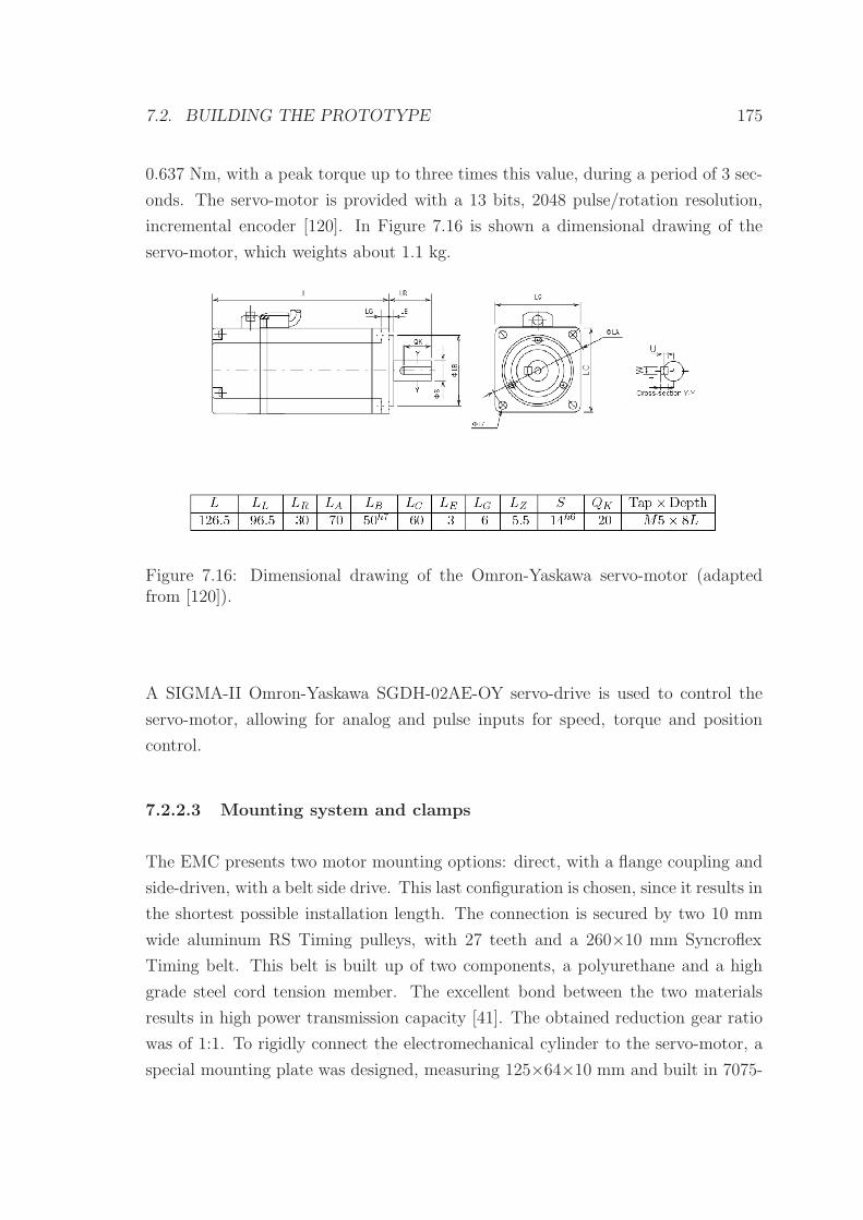
7.2. BUILDING THE PROTOTYPE 175
0.637 Nm, with a peak torque up to three times this value, during a period of 3 sec-
onds. The servo-motor is provided with a 13 bits, 2048 pulse/rotation resolution,
incremental encoder [120]. In Figure 7.16 is shown a dimensional drawing of the
servo-motor, which weights about 1.1 kg.
Figure 7.16: Dimensional drawing of the Omron-Yaskawa servo-motor (adaptedfrom [120]).
A SIGMA-II Omron-Yaskawa SGDH-02AE-OY servo-drive is used to control the
servo-motor, allowing for analog and pulse inputs for speed, torque and position
control.
7.2.2.3 Mounting system and clamps
The EMC presents two motor mounting options: direct, with a flange coupling and
side-driven, with a belt side drive. This last configuration is chosen, since it results in
the shortest possible installation length. The connection is secured by two 10 mm
wide aluminum RS Timing pulleys, with 27 teeth and a 260×10 mm Syncroflex
Timing belt. This belt is built up of two components, a polyurethane and a high
grade steel cord tension member. The excellent bond between the two materials
results in high power transmission capacity [41]. The obtained reduction gear ratio
was of 1:1. To rigidly connect the electromechanical cylinder to the servo-motor, a
special mounting plate was designed, measuring 125×64×10 mm and built in 7075-
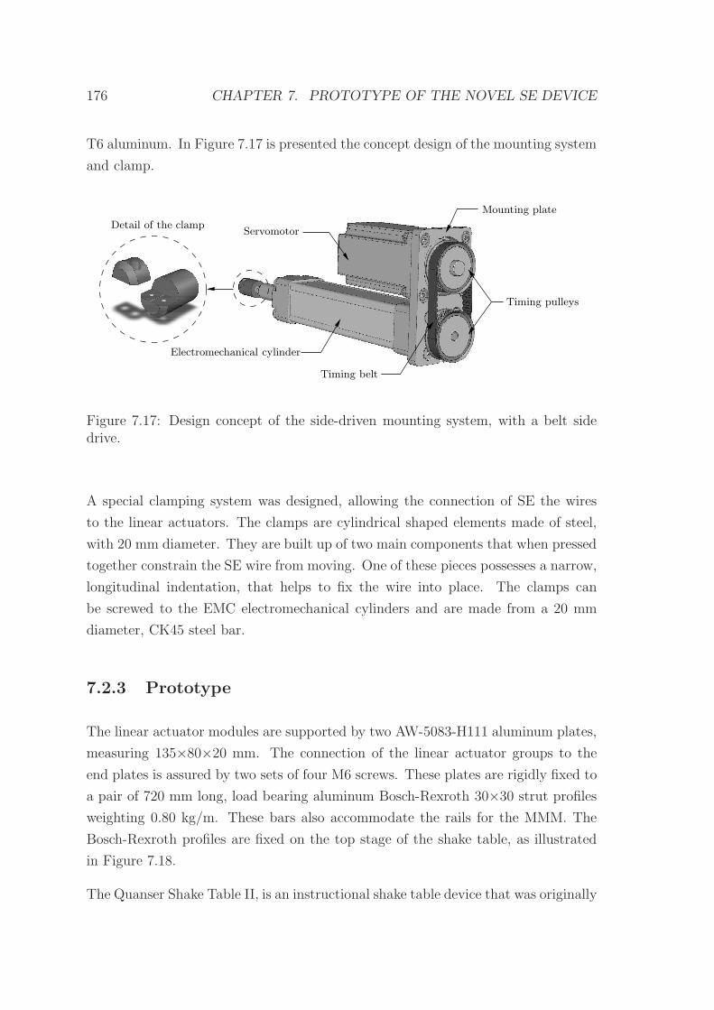
176 CHAPTER 7. PROTOTYPE OF THE NOVEL SE DEVICE
T6 aluminum. In Figure 7.17 is presented the concept design of the mounting system
and clamp.
Servomotor
Timing pulleys
Mounting plate
Detail of the clamp
Electromechanical cylinder
Timing belt
Figure 7.17: Design concept of the side-driven mounting system, with a belt sidedrive.
A special clamping system was designed, allowing the connection of SE the wires
to the linear actuators. The clamps are cylindrical shaped elements made of steel,
with 20 mm diameter. They are built up of two main components that when pressed
together constrain the SE wire from moving. One of these pieces possesses a narrow,
longitudinal indentation, that helps to fix the wire into place. The clamps can
be screwed to the EMC electromechanical cylinders and are made from a 20 mm
diameter, CK45 steel bar.
7.2.3 Prototype
The linear actuator modules are supported by two AW-5083-H111 aluminum plates,
measuring 135×80×20 mm. The connection of the linear actuator groups to the
end plates is assured by two sets of four M6 screws. These plates are rigidly fixed to
a pair of 720 mm long, load bearing aluminum Bosch-Rexroth 30×30 strut profiles
weighting 0.80 kg/m. These bars also accommodate the rails for the MMM. The
Bosch-Rexroth profiles are fixed on the top stage of the shake table, as illustrated
in Figure 7.18.
The Quanser Shake Table II, is an instructional shake table device that was originally
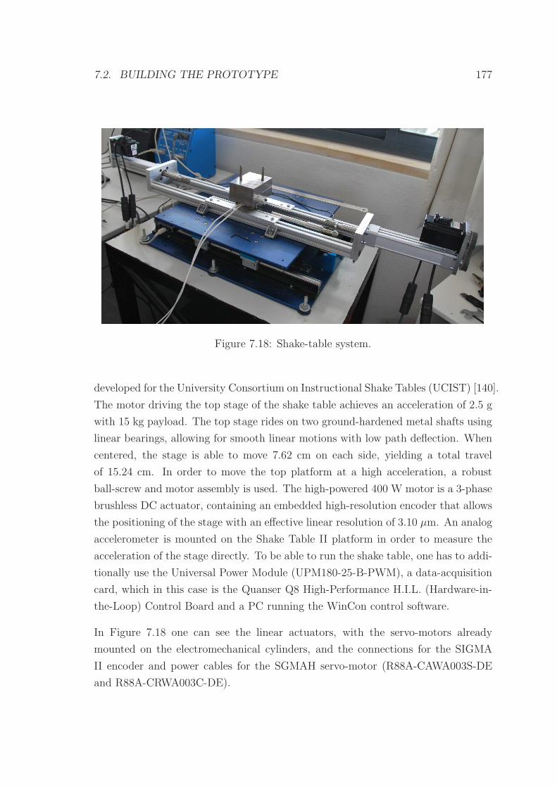
7.2. BUILDING THE PROTOTYPE 177
Figure 7.18: Shake-table system.
developed for the University Consortium on Instructional Shake Tables (UCIST) [140].
The motor driving the top stage of the shake table achieves an acceleration of 2.5 g
with 15 kg payload. The top stage rides on two ground-hardened metal shafts using
linear bearings, allowing for smooth linear motions with low path deflection. When
centered, the stage is able to move 7.62 cm on each side, yielding a total travel
of 15.24 cm. In order to move the top platform at a high acceleration, a robust
ball-screw and motor assembly is used. The high-powered 400 W motor is a 3-phase
brushless DC actuator, containing an embedded high-resolution encoder that allows
the positioning of the stage with an effective linear resolution of 3.10 µm. An analog
accelerometer is mounted on the Shake Table II platform in order to measure the
acceleration of the stage directly. To be able to run the shake table, one has to addi-
tionally use the Universal Power Module (UPM180-25-B-PWM), a data-acquisition
card, which in this case is the Quanser Q8 High-Performance H.I.L. (Hardware-in-
the-Loop) Control Board and a PC running the WinCon control software.
In Figure 7.18 one can see the linear actuators, with the servo-motors already
mounted on the electromechanical cylinders, and the connections for the SIGMA
II encoder and power cables for the SGMAH servo-motor (R88A-CAWA003S-DE
and R88A-CRWA003C-DE).
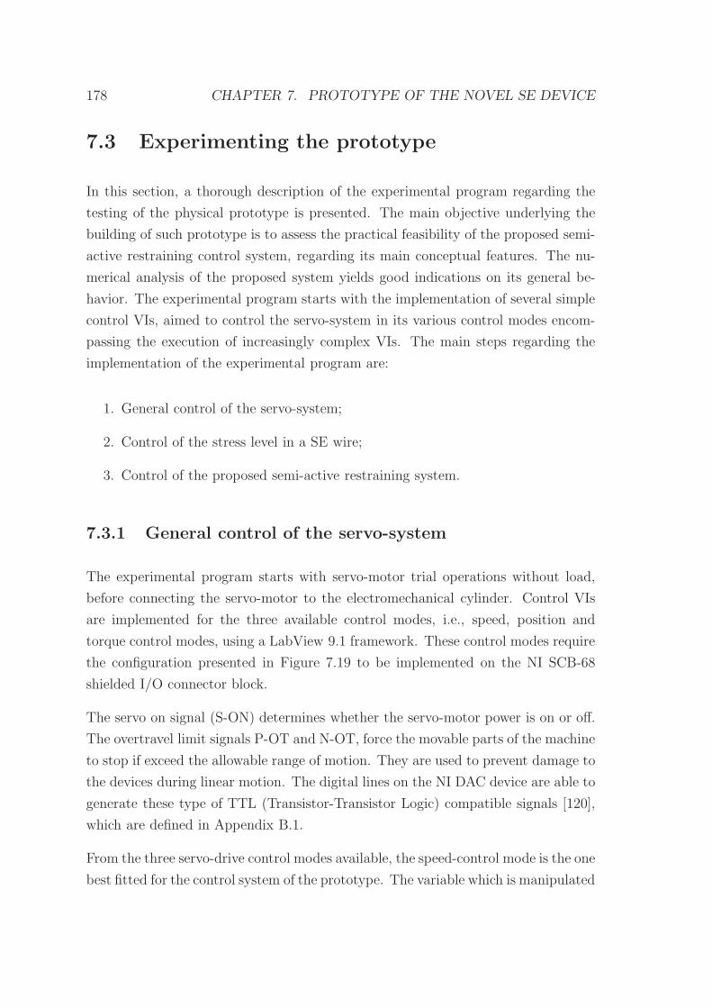
178 CHAPTER 7. PROTOTYPE OF THE NOVEL SE DEVICE
7.3 Experimenting the prototype
In this section, a thorough description of the experimental program regarding the
testing of the physical prototype is presented. The main objective underlying the
building of such prototype is to assess the practical feasibility of the proposed semi-
active restraining control system, regarding its main conceptual features. The nu-
merical analysis of the proposed system yields good indications on its general be-
havior. The experimental program starts with the implementation of several simple
control VIs, aimed to control the servo-system in its various control modes encom-
passing the execution of increasingly complex VIs. The main steps regarding the
implementation of the experimental program are:
1. General control of the servo-system;
2. Control of the stress level in a SE wire;
3. Control of the proposed semi-active restraining system.
7.3.1 General control of the servo-system
The experimental program starts with servo-motor trial operations without load,
before connecting the servo-motor to the electromechanical cylinder. Control VIs
are implemented for the three available control modes, i.e., speed, position and
torque control modes, using a LabView 9.1 framework. These control modes require
the configuration presented in Figure 7.19 to be implemented on the NI SCB-68
shielded I/O connector block.
The servo on signal (S-ON) determines whether the servo-motor power is on or off.
The overtravel limit signals P-OT and N-OT, force the movable parts of the machine
to stop if exceed the allowable range of motion. They are used to prevent damage to
the devices during linear motion. The digital lines on the NI DAC device are able to
generate these type of TTL (Transistor-Transistor Logic) compatible signals [120],
which are defined in Appendix B.1.
From the three servo-drive control modes available, the speed-control mode is the one
best fitted for the control system of the prototype. The variable which is manipulated
7.3. EXPERIMENTING THE PROTOTYPE 179
(a) Speed-control. (b) Position-control. (c) Torque-control.
Figure 7.19: Simplified external input signal circuits for the servosystem controlmodes, with corresponding connector pin (adapted from [120]).
by the controller is the analog voltage level for the servo-drive’s speed reference (V-
REF).
7.3.1.1 Speed-control mode
The maximum analog voltage level for the speed reference, is set to 6 V, which is
equivalent to the rated speed of the servo-motor (3000 rpm). The analog voltage
signal is a bipolar signal, with a range that includes both positive and negative
values, in order to be able to change the travel direction of the shaft of the servo-
motor. The internal voltage reference of the DAC is calibrated to the same range
as the signal (-6 to +6 V), in order to maximize the DAC resolution. A VI that
generates a variable voltage is built, which is able to continuously update the analog
output channel. The block diagram of this VI is presented in Figure 7.20.
Both the analog output voltage channel, to control the speed of the servo-motor (V-
REF), as well as the digital output channel, which controls all the digital channels
(S-ON, P-OT and N-OT) can be seen in the block diagram of the speed-control VI.
In appendix B.2 is also presented the implementation of a VI for the position-control
mode. The specifications for the servo-drive are presented in appendix B.3.
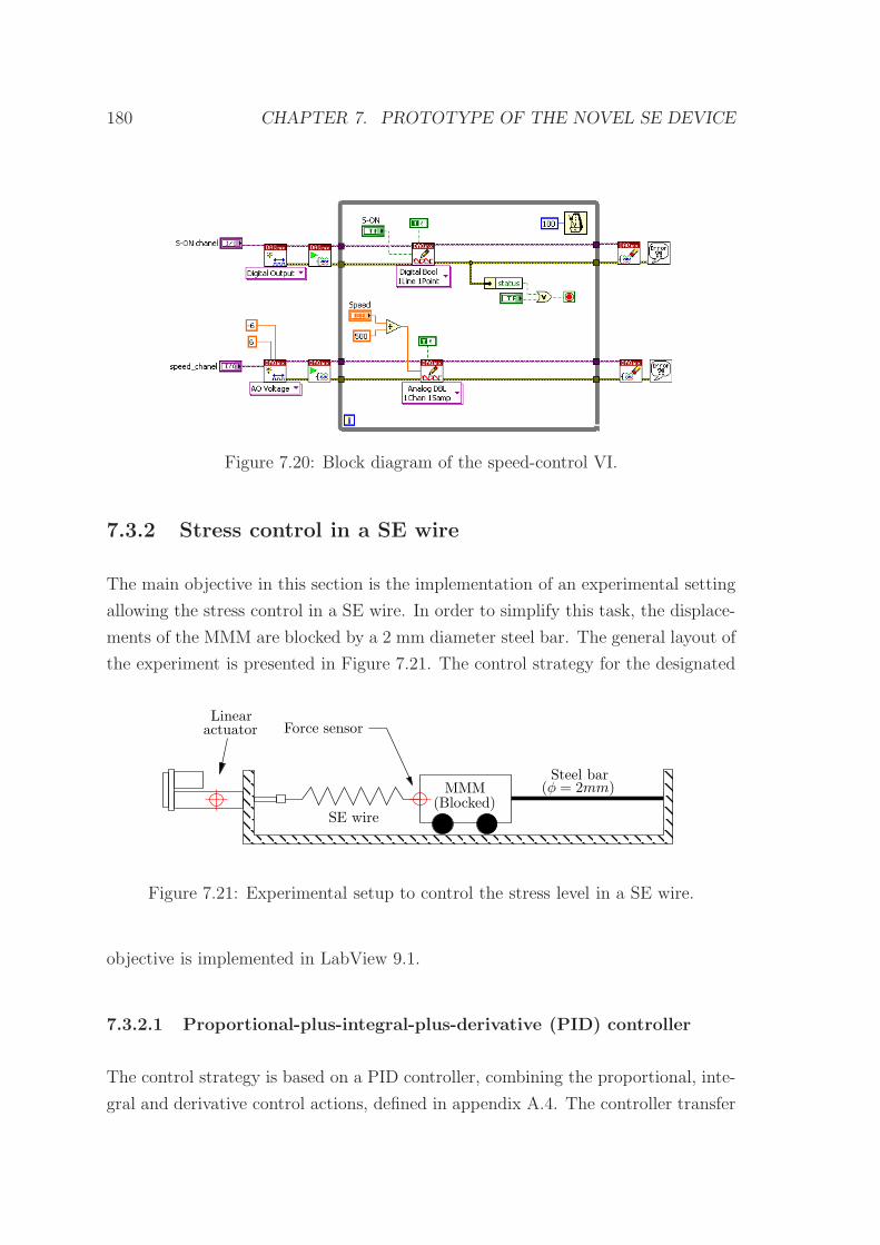
180 CHAPTER 7. PROTOTYPE OF THE NOVEL SE DEVICE
Figure 7.20: Block diagram of the speed-control VI.
7.3.2 Stress control in a SE wire
The main objective in this section is the implementation of an experimental setting
allowing the stress control in a SE wire. In order to simplify this task, the displace-
ments of the MMM are blocked by a 2 mm diameter steel bar. The general layout of
the experiment is presented in Figure 7.21. The control strategy for the designated
MMM
actuatorLinear
Steel bar(φ = 2mm)
(Blocked)
Force sensor
SE wire
Figure 7.21: Experimental setup to control the stress level in a SE wire.
objective is implemented in LabView 9.1.
7.3.2.1 Proportional-plus-integral-plus-derivative (PID) controller
The control strategy is based on a PID controller, combining the proportional, inte-
gral and derivative control actions, defined in appendix A.4. The controller transfer
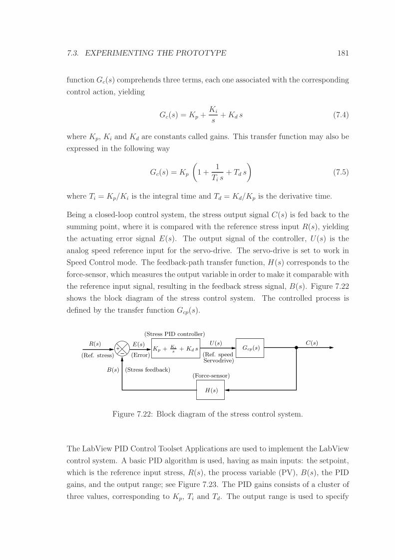
7.3. EXPERIMENTING THE PROTOTYPE 181
function Gc(s) comprehends three terms, each one associated with the corresponding
control action, yielding
Gc(s) = Kp +Ki
s+Kd s (7.4)
where Kp, Ki and Kd are constants called gains. This transfer function may also be
expressed in the following way
Gc(s) = Kp
(
1 +1
Ti s+ Td s
)
(7.5)
where Ti = Kp/Ki is the integral time and Td = Kd/Kp is the derivative time.
Being a closed-loop control system, the stress output signal C(s) is fed back to the
summing point, where it is compared with the reference stress input R(s), yielding
the actuating error signal E(s). The output signal of the controller, U(s) is the
analog speed reference input for the servo-drive. The servo-drive is set to work in
Speed Control mode. The feedback-path transfer function, H(s) corresponds to the
force-sensor, which measures the output variable in order to make it comparable with
the reference input signal, resulting in the feedback stress signal, B(s). Figure 7.22
shows the block diagram of the stress control system. The controlled process is
defined by the transfer function Gcp(s).
+
H(s)
R(s) E(s) C(s)
(Force-sensor)
Gcp(s)
(Ref. stress)
B(s)
U(s)
(Error)
(Stress feedback)
(Stress PID controller)
Kp + Ki
s+ Kd s
(Ref. speedServodrive)
Figure 7.22: Block diagram of the stress control system.
The LabView PID Control Toolset Applications are used to implement the LabView
control system. A basic PID algorithm is used, having as main inputs: the setpoint,
which is the reference input stress, R(s), the process variable (PV), B(s), the PID
gains, and the output range; see Figure 7.23. The PID gains consists of a cluster of
three values, corresponding to Kp, Ti and Td. The output range is used to specify
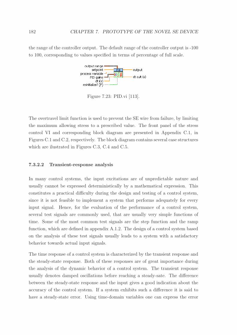
182 CHAPTER 7. PROTOTYPE OF THE NOVEL SE DEVICE
the range of the controller output. The default range of the controller output is -100
to 100, corresponding to values specified in terms of percentage of full scale.
Figure 7.23: PID.vi [113].
The overtravel limit function is used to prevent the SE wire from failure, by limiting
the maximum allowing stress to a prescribed value. The front panel of the stress
control VI and corresponding block diagram are presented in Appendix C.1, in
Figures C.1 and C.2, respectively. The block diagram contains several case structures
which are ilustrated in Figures C.3, C.4 and C.5.
7.3.2.2 Transient-response analysis
In many control systems, the input excitations are of unpredictable nature and
usually cannot be expressed deterministically by a mathematical expression. This
constitutes a practical difficulty during the design and testing of a control system,
since it is not feasible to implement a system that performs adequately for every
input signal. Hence, for the evaluation of the performance of a control system,
several test signals are commonly used, that are usually very simple functions of
time. Some of the most common test signals are the step function and the ramp
function, which are defined in appendix A.1.2. The design of a control system based
on the analysis of these test signals usually leads to a system with a satisfactory
behavior towards actual input signals.
The time response of a control system is characterized by the transient response and
the steady-state response. Both of these responses are of great importance during
the analysis of the dynamic behavior of a control system. The transient response
usually denotes damped oscillations before reaching a steady-sate. The difference
between the steady-state response and the input gives a good indication about the
accuracy of the control system. If a system exhibits such a difference it is said to
have a steady-state error. Using time-domain variables one can express the error
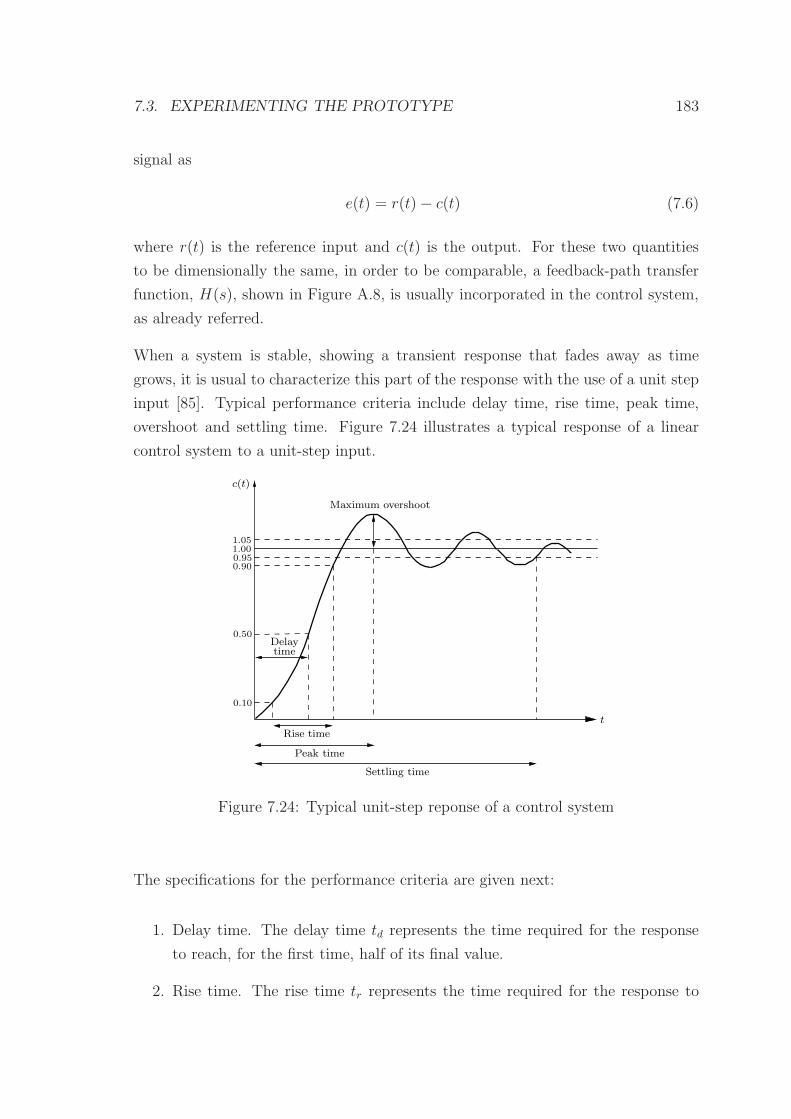
7.3. EXPERIMENTING THE PROTOTYPE 183
signal as
e(t) = r(t)− c(t) (7.6)
where r(t) is the reference input and c(t) is the output. For these two quantities
to be dimensionally the same, in order to be comparable, a feedback-path transfer
function, H(s), shown in Figure A.8, is usually incorporated in the control system,
as already referred.
When a system is stable, showing a transient response that fades away as time
grows, it is usual to characterize this part of the response with the use of a unit step
input [85]. Typical performance criteria include delay time, rise time, peak time,
overshoot and settling time. Figure 7.24 illustrates a typical response of a linear
control system to a unit-step input.
1.051.00
0.90
0.50
0.10
0.95
Delay
c(t)
time
Settling time
Peak time
Rise time
t
Maximum overshoot
Figure 7.24: Typical unit-step reponse of a control system
The specifications for the performance criteria are given next:
1. Delay time. The delay time td represents the time required for the response
to reach, for the first time, half of its final value.
2. Rise time. The rise time tr represents the time required for the response to
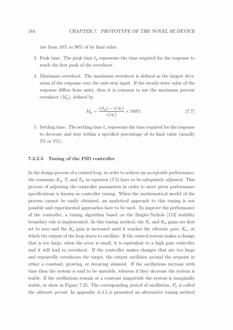
184 CHAPTER 7. PROTOTYPE OF THE NOVEL SE DEVICE
rise from 10% to 90% of its final value.
3. Peak time. The peak time tp represents the time required for the response to
reach the first peak of the overshoot.
4. Maximum overshoot. The maximum overshoot is defined as the largest devi-
ation of the response over the unit-step input. If the steady-state value of the
response differs from unity, then it is common to use the maximum percent
overshoot (Mp), defined by
Mp =c(tp)− c(∞)
c(∞)× 100% (7.7)
5. Settling time. The settling time ts represents the time required for the response
to decrease and stay within a specified percentage of its final value (usually
2% or 5%).
7.3.2.3 Tuning of the PID controller
In the design process of a control loop, in order to achieve an acceptable performance,
the constants Kp, Ti and Td, in equation (7.5) have to be adequately adjusted. This
process of adjusting the controller parameters in order to meet given performance
specifications is known as controller tuning. When the mathematical model of the
process cannot be easily obtained, an analytical approach to this tuning is not
possible and experimental approaches have to be used. To improve the performance
of the controller, a tuning algorithm based on the Ziegler-Nichols [113] stability
boundary rule is implemented. In this tuning method, the Ki and Kd gains are first
set to zero and the Kp gain is increased until it reaches the ultimate gain, Ku, at
which the output of the loop starts to oscillate. If the control system makes a change
that is too large, when the error is small, it is equivalent to a high gain controller
and it will lead to overshoot. If the controller makes changes that are too large
and repeatedly overshoots the target, the output oscillates around the setpoint in
either a constant, growing, or decaying sinusoid. If the oscillations increase with
time then the system is said to be unstable, whereas if they decrease the system is
stable. If the oscillations remain at a constant magnitude the system is marginally
stable, as show in Figure 7.25. The corresponding period of oscillation, Pu is called
the ultimate period. In appendix A.4.5 is presented an alternative tuning method
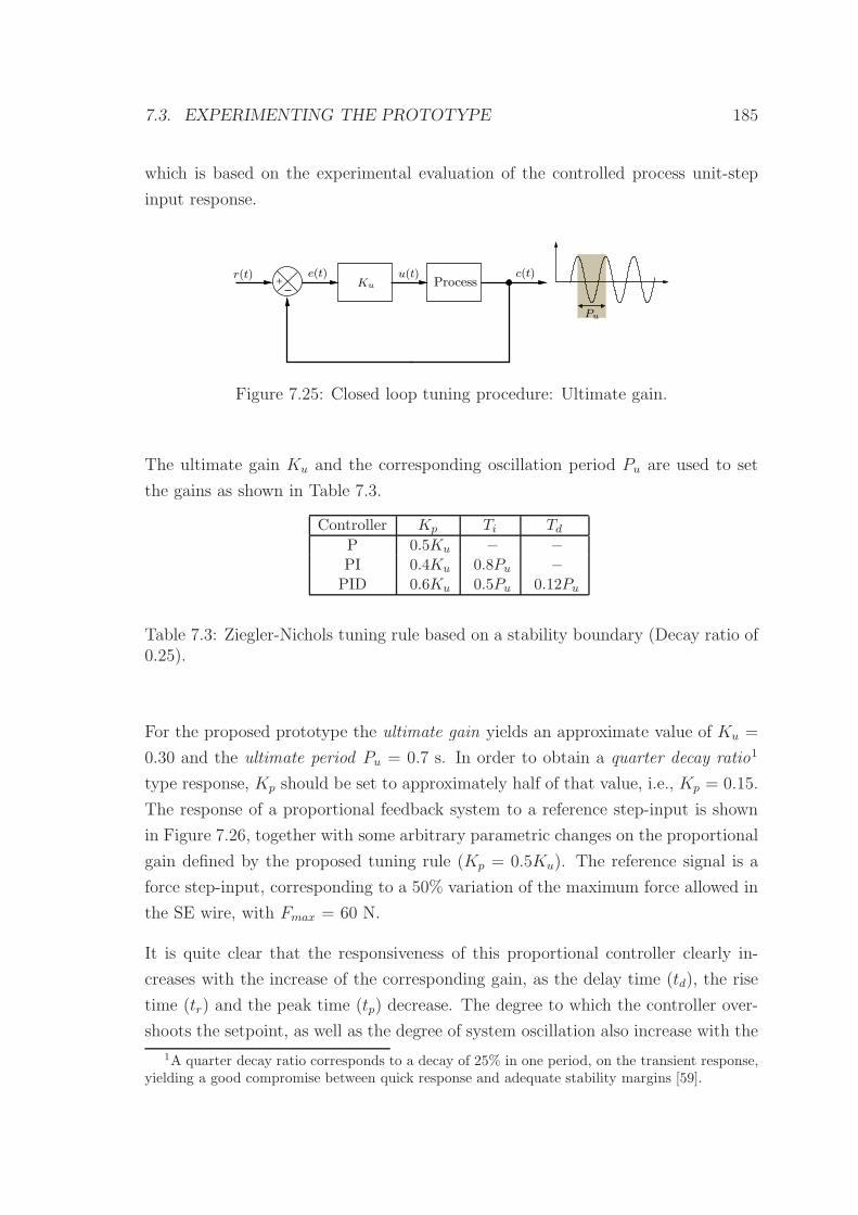
7.3. EXPERIMENTING THE PROTOTYPE 185
which is based on the experimental evaluation of the controlled process unit-step
input response.
+r(t) e(t)
Processc(t)
Ku
Pu
u(t)
Figure 7.25: Closed loop tuning procedure: Ultimate gain.
The ultimate gain Ku and the corresponding oscillation period Pu are used to set
the gains as shown in Table 7.3.
Controller Kp Ti Td
P 0.5Ku − −PI 0.4Ku 0.8Pu −PID 0.6Ku 0.5Pu 0.12Pu
Table 7.3: Ziegler-Nichols tuning rule based on a stability boundary (Decay ratio of0.25).
For the proposed prototype the ultimate gain yields an approximate value of Ku =
0.30 and the ultimate period Pu = 0.7 s. In order to obtain a quarter decay ratio1
type response, Kp should be set to approximately half of that value, i.e., Kp = 0.15.
The response of a proportional feedback system to a reference step-input is shown
in Figure 7.26, together with some arbitrary parametric changes on the proportional
gain defined by the proposed tuning rule (Kp = 0.5Ku). The reference signal is a
force step-input, corresponding to a 50% variation of the maximum force allowed in
the SE wire, with Fmax = 60 N.
It is quite clear that the responsiveness of this proportional controller clearly in-
creases with the increase of the corresponding gain, as the delay time (td), the rise
time (tr) and the peak time (tp) decrease. The degree to which the controller over-
shoots the setpoint, as well as the degree of system oscillation also increase with the
1A quarter decay ratio corresponds to a decay of 25% in one period, on the transient response,yielding a good compromise between quick response and adequate stability margins [59].
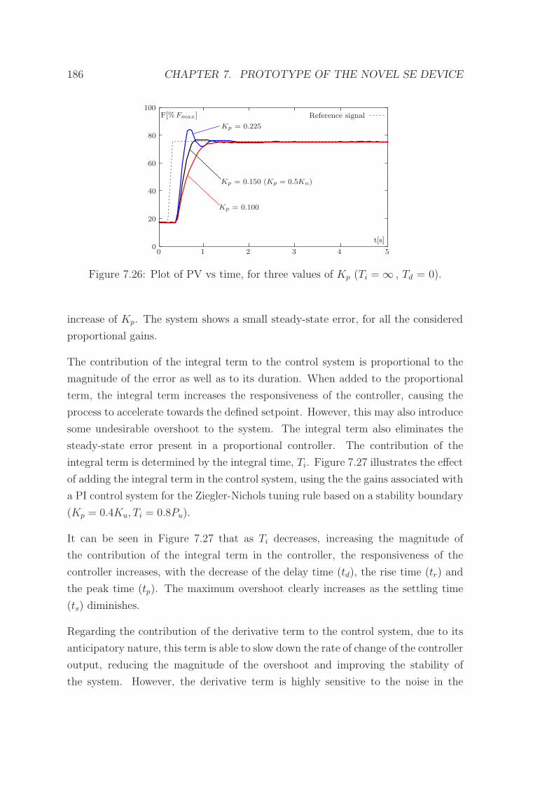
186 CHAPTER 7. PROTOTYPE OF THE NOVEL SE DEVICE
Reference signal
t[s]
50 1 2 3 4
80
60
40
20
0
Kp = 0.225
Kp = 0.100
F[%Fmax]100
Kp = 0.150 (Kp = 0.5Ku)
Figure 7.26: Plot of PV vs time, for three values of Kp (Ti = ∞ , Td = 0).
increase of Kp. The system shows a small steady-state error, for all the considered
proportional gains.
The contribution of the integral term to the control system is proportional to the
magnitude of the error as well as to its duration. When added to the proportional
term, the integral term increases the responsiveness of the controller, causing the
process to accelerate towards the defined setpoint. However, this may also introduce
some undesirable overshoot to the system. The integral term also eliminates the
steady-state error present in a proportional controller. The contribution of the
integral term is determined by the integral time, Ti. Figure 7.27 illustrates the effect
of adding the integral term in the control system, using the the gains associated with
a PI control system for the Ziegler-Nichols tuning rule based on a stability boundary
(Kp = 0.4Ku, Ti = 0.8Pu).
It can be seen in Figure 7.27 that as Ti decreases, increasing the magnitude of
the contribution of the integral term in the controller, the responsiveness of the
controller increases, with the decrease of the delay time (td), the rise time (tr) and
the peak time (tp). The maximum overshoot clearly increases as the settling time
(ts) diminishes.
Regarding the contribution of the derivative term to the control system, due to its
anticipatory nature, this term is able to slow down the rate of change of the controller
output, reducing the magnitude of the overshoot and improving the stability of
the system. However, the derivative term is highly sensitive to the noise in the
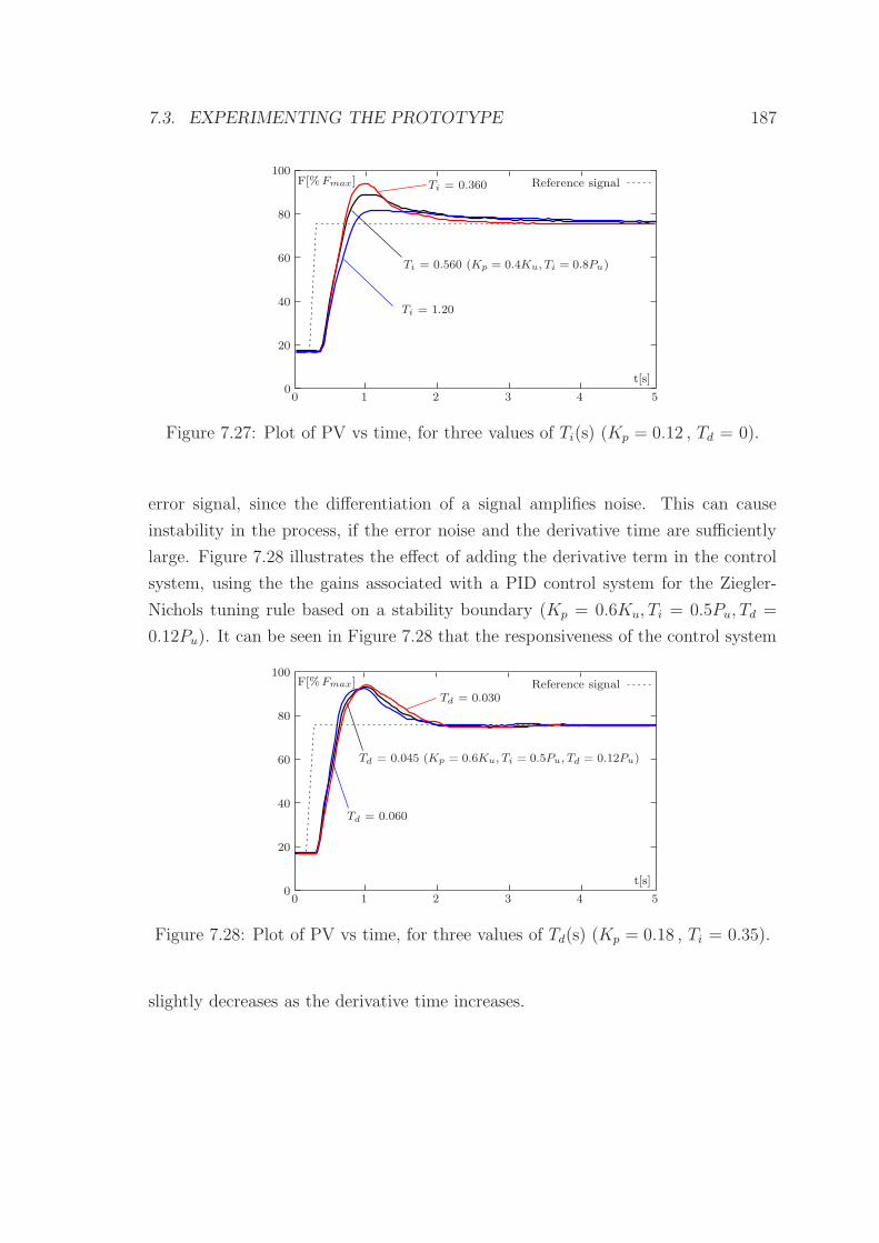
7.3. EXPERIMENTING THE PROTOTYPE 187
Reference signal100
t[s]
50 1 2 3 4
80
60
40
20
0
F[%Fmax] Ti = 0.360
Ti = 1.20
Ti = 0.560 (Kp = 0.4Ku, Ti = 0.8Pu)
Figure 7.27: Plot of PV vs time, for three values of Ti(s) (Kp = 0.12 , Td = 0).
error signal, since the differentiation of a signal amplifies noise. This can cause
instability in the process, if the error noise and the derivative time are sufficiently
large. Figure 7.28 illustrates the effect of adding the derivative term in the control
system, using the the gains associated with a PID control system for the Ziegler-
Nichols tuning rule based on a stability boundary (Kp = 0.6Ku, Ti = 0.5Pu, Td =
0.12Pu). It can be seen in Figure 7.28 that the responsiveness of the control system
Reference signal100
t[s]
50 1 2 3 4
80
60
40
20
0
F[%Fmax]
Td = 0.045 (Kp = 0.6Ku, Ti = 0.5Pu, Td = 0.12Pu)
Td = 0.030
Td = 0.060
Figure 7.28: Plot of PV vs time, for three values of Td(s) (Kp = 0.18 , Ti = 0.35).
slightly decreases as the derivative time increases.
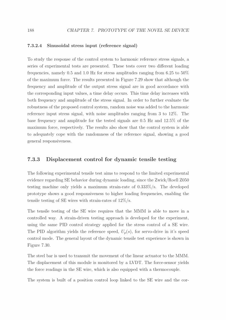
188 CHAPTER 7. PROTOTYPE OF THE NOVEL SE DEVICE
7.3.2.4 Sinusoidal stress input (reference signal)
To study the response of the control system to harmonic reference stress signals, a
series of experimental tests are presented. These tests cover two different loading
frequencies, namely 0.5 and 1.0 Hz for stress amplitudes ranging from 6.25 to 50%
of the maximum force. The results presented in Figure 7.29 show that although the
frequency and amplitude of the output stress signal are in good accordance with
the corresponding input values, a time delay occurs. This time delay increases with
both frequency and amplitude of the stress signal. In order to further evaluate the
robustness of the proposed control system, random noise was added to the harmonic
reference input stress signal, with noise amplitudes ranging from 3 to 12%. The
base frequency and amplitude for the tested signals are 0.5 Hz and 12.5% of the
maximum force, respectively. The results also show that the control system is able
to adequately cope with the randomness of the reference signal, showing a good
general responsiveness.
7.3.3 Displacement control for dynamic tensile testing
The following experimental tensile test aims to respond to the limited experimental
evidence regarding SE behavior during dynamic loading, since the Zwick/Roell Z050
testing machine only yields a maximum strain-rate of 0.333%/s. The developed
prototype shows a good responsiveness to higher loading frequencies, enabling the
tensile testing of SE wires with strain-rates of 12%/s.
The tensile testing of the SE wire requires that the MMM is able to move in a
controlled way. A strain-driven testing approach is developed for the experiment,
using the same PID control strategy applied for the stress control of a SE wire.
The PID algorithm yields the reference speed, Up(s), for servo-drive in it’s speed
control mode. The general layout of the dynamic tensile test experience is shown in
Figure 7.30.
The steel bar is used to transmit the movement of the linear actuator to the MMM.
The displacement of this module is monitored by a LVDT. The force-sensor yields
the force readings in the SE wire, which is also equipped with a thermocouple.
The system is built of a position control loop linked to the SE wire and the cor-
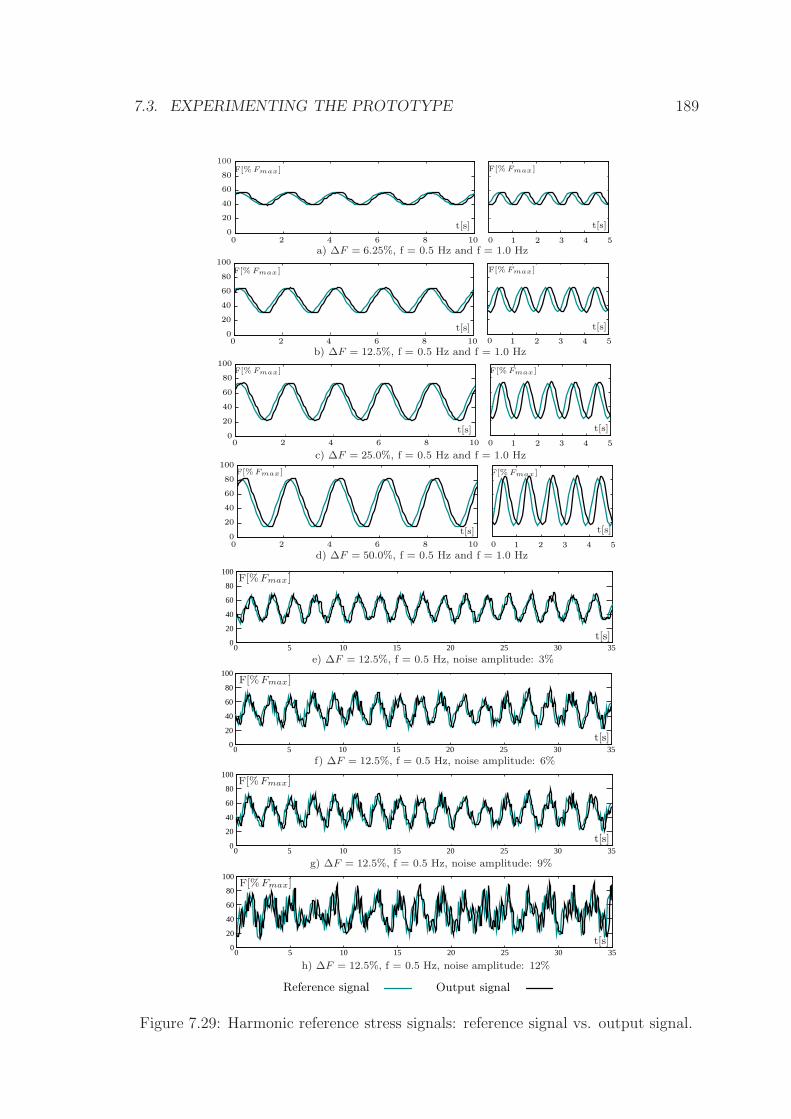
7.3. EXPERIMENTING THE PROTOTYPE 189
0 5 10 15 20 25 30 35
0 5 10 15 20 25 30 35
0 5 10 15 20 25 30 35
100
80
60
40
20
0
100
80
60
40
20
0
100
80
60
40
20
0
100
80
60
40
20
0
0 5 10 15 20 25 30 35
Reference signal Output signal
10420 86 1 2 3 4 50
100
80
60
40
20
0
10420 86 1 2 3 4 50
100
80
60
40
20
0
1 2 3 4 5010420 86
100
80
60
40
20
0
10420 86 1 2 3 4 50
80
60
40
20
0
t[s] t[s]
F[%Fmax] F[%Fmax]
t[s] t[s]
F[%Fmax] F[%Fmax]
t[s] t[s]
F[%Fmax]F[%Fmax]
F[%Fmax]
t[s]
F[%Fmax]
F[%Fmax]
F[%Fmax]
t[s]
t[s]
t[s]
e) ∆F = 12.5%, f = 0.5 Hz, noise amplitude: 3%
f) ∆F = 12.5%, f = 0.5 Hz, noise amplitude: 6%
g) ∆F = 12.5%, f = 0.5 Hz, noise amplitude: 9%
h) ∆F = 12.5%, f = 0.5 Hz, noise amplitude: 12%
a) ∆F = 6.25%, f = 0.5 Hz and f = 1.0 Hz
b) ∆F = 12.5%, f = 0.5 Hz and f = 1.0 Hz
c) ∆F = 25.0%, f = 0.5 Hz and f = 1.0 Hz
d) ∆F = 50.0%, f = 0.5 Hz and f = 1.0 Hz
t[s] t[s]
F[%Fmax] F[%Fmax]100
Figure 7.29: Harmonic reference stress signals: reference signal vs. output signal.
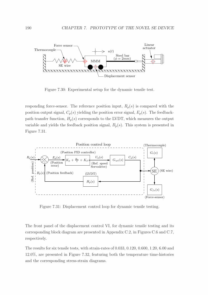
190 CHAPTER 7. PROTOTYPE OF THE NOVEL SE DEVICE
MMM
actuatorLinear
Displacement sensor
u(t)Steel bar
(φ = 2mm)
Thermocouple
SE wire
Force sensor
Figure 7.30: Experimental setup for the dynamic tensile test.
responding force-sensor. The reference position input, Rp(s) is compared with the
position output signal, Cp(s) yielding the position error signal, Ep(s). The feedback-
path transfer function, Hp(s) corresponds to the LVDT, which measures the output
variable and yields the feedback position signal, Bp(s). This system is presented in
Figure 7.31.
+
SE
(Position PID controller)
Up(s) Cp(s)
(Positionerror)
(Position feedback)
Ep(s)
Hp(s)
Gcp1(s)(Ref. speed
(LVDT)Bp(s)
Rp(s)
(Ref.position)
Servodrive)
(SE wire)
(Thermocouple)
Gt(s)
(Force-sensor)
Gfs(s)
Position control loop
Kp + Ki
s+ Kd s
Figure 7.31: Displacement control loop for dynamic tensile testing.
The front panel of the displacement control VI, for dynamic tensile testing and its
corresponding block diagram are presented in Appendix C.2, in Figures C.6 and C.7,
respectively.
The results for six tensile tests, with strain-rates of 0.033, 0.120, 0.600, 1.20, 6.00 and
12.0%, are presented in Figure 7.32, featuring both the temperature time-histories
and the corresponding stress-strain diagrams.
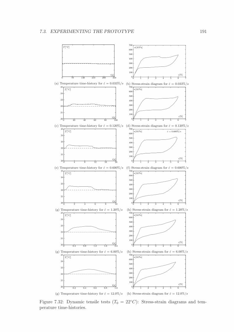
7.3. EXPERIMENTING THE PROTOTYPE 191
0 35070 140 280210
T [C]
t[s]
(a) Temperature time-history for ε = 0.033%/s
700
600
500
400
300
200
100
010 2 3 4 5 6 7
σ[MPa]
ε[%]
(b) Stress-strain diagram for ε = 0.033%/s25
24
23
22
21
200 10020 40 60 80
T [C]
t[s]
(c) Temperature time-history for ε = 0.120%/s
700
600
500
400
300
200
100
010 2 3 4 5 6 7
ε[%]
σ[MPa]
(d) Stress-strain diagram for ε = 0.120%/s25
24
23
22
21
200 20161284
T [C]
t[s]
(e) Temperature time-history for ε = 0.600%/s
700
600
500
400
300
200
100
00 1 2 3 4 5 6 7
ε[%]
σ[MPa] ε = 0.600%/s
(f) Stress-strain diagram for ε = 0.600%/s25
24
23
22
21
200 2 4 6 8 10
T [C]
t[s]
(g) Temperature time-history for ε = 1.20%/s
700
600
500
400
300
200
100
00 1 2 3 4 5 6 7
ε[%]
σ[MPa]
(h) Stress-strain diagram for ε = 1.20%/s25
24
23
22
21
200 1.6 2.01.20.80.4
T [C]
t[s]
(g) Temperature time-history for ε = 6.00%/s
700
600
500
400
300
200
100
00 1 2 3 4 5 6 7
ε[%]
σ[MPa]
(h) Stress-strain diagram for ε = 6.00%/s25
24
23
22
21
200 1.00.80.60.40.2
T [C]
t[s]
(g) Temperature time-history for ε = 12.0%/s
700
600
500
400
300
200
100
00 1 2 3 4 5 6 7
ε[%]
σ[MPa]
(h) Stress-strain diagram for ε = 12.0%/s
Figure 7.32: Dynamic tensile tests (T0 = 22C): Stress-strain diagrams and tem-perature time-histories.
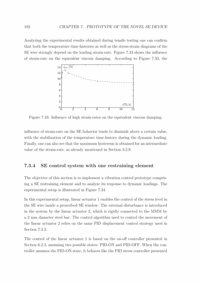
192 CHAPTER 7. PROTOTYPE OF THE NOVEL SE DEVICE
Analyzing the experimental results obtained during tensile testing one can confirm
that both the temperature time-histories as well as the stress-strain diagrams of the
SE wire strongly depend on the loading strain-rate. Figure 7.33 shows the influence
of strain-rate on the equivalent viscous damping. According to Figure 7.33, the
0 2 4 6 8 10 12
ε[%/s]
14
12
10
8
6
4
2
0
ζeq [%]
Figure 7.33: Influence of high strain-rates on the equivalent viscous damping.
influence of strain-rate on the SE behavior tends to diminish above a certain value,
with the stabilization of the temperature time-history during the dynamic loading.
Finally, one can also see that the maximum hysteresis is obtained for an intermediate
value of the strain-rate, as already mentioned in Section 3.2.9.
7.3.4 SE control system with one restraining element
The objective of this section is to implement a vibration control prototype compris-
ing a SE restraining element and to analyze its response to dynamic loadings. The
experimental setup is illustrated in Figure 7.34.
In this experimental setup, linear actuator 1 enables the control of the stress level in
the SE wire inside a prescribed SE window. The external disturbance is introduced
in the system by the linear actuator 2, which is rigidly connected to the MMM by
a 2 mm diameter steel bar. The control algorithm used to control the movement of
the linear actuator 2 relies on the same PID displacement control strategy used in
Section 7.3.3.
The control of the linear actuator 1 is based on the on-off controller presented in
Section 6.2.3, assuming two possible states: PID-ON and PID-OFF. When the con-
troller assumes the PID-ON state, it behaves like the PID stress controller presented
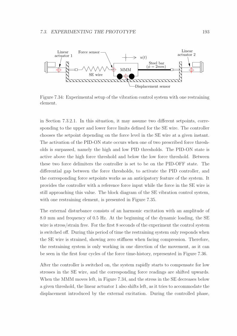
7.3. EXPERIMENTING THE PROTOTYPE 193
MMM
u(t)actuator 2
Linearactuator 1Linear
Steel bar(φ = 2mm)
Displacement sensor
SE wire
Force sensor
Figure 7.34: Experimental setup of the vibration control system with one restrainingelement.
in Section 7.3.2.1. In this situation, it may assume two different setpoints, corre-
sponding to the upper and lower force limits defined for the SE wire. The controller
chooses the setpoint depending on the force level in the SE wire at a given instant.
The activation of the PID-ON state occurs when one of two prescribed force thresh-
olds is surpassed, namely the high and low PID thresholds. The PID-ON state is
active above the high force threshold and below the low force threshold. Between
these two force delimiters the controller is set to be on the PID-OFF state. The
differential gap between the force thresholds, to activate the PID controller, and
the corresponding force setpoints works as an anticipatory feature of the system. It
provides the controller with a reference force input while the force in the SE wire is
still approaching this value. The block diagram of the SE vibration control system,
with one restraining element, is presented in Figure 7.35.
The external disturbance consists of an harmonic excitation with an amplitude of
8.0 mm and frequency of 0.5 Hz. At the beginning of the dynamic loading, the SE
wire is stress/strain free. For the first 8 seconds of the experiment the control system
is switched off. During this period of time the restraining system only responds when
the SE wire is strained, showing zero stiffness when facing compression. Therefore,
the restraining system is only working in one direction of the movement, as it can
be seen in the first four cycles of the force time-history, represented in Figure 7.36.
After the controller is switched on, the system rapidly starts to compensate for low
stresses in the SE wire, and the corresponding force readings are shifted upwards.
When the MMM moves left, in Figure 7.34, and the stress in the SE decreases below
a given threshold, the linear actuator 1 also shifts left, as it tries to accommodate the
displacement introduced by the external excitation. During the controlled phase,
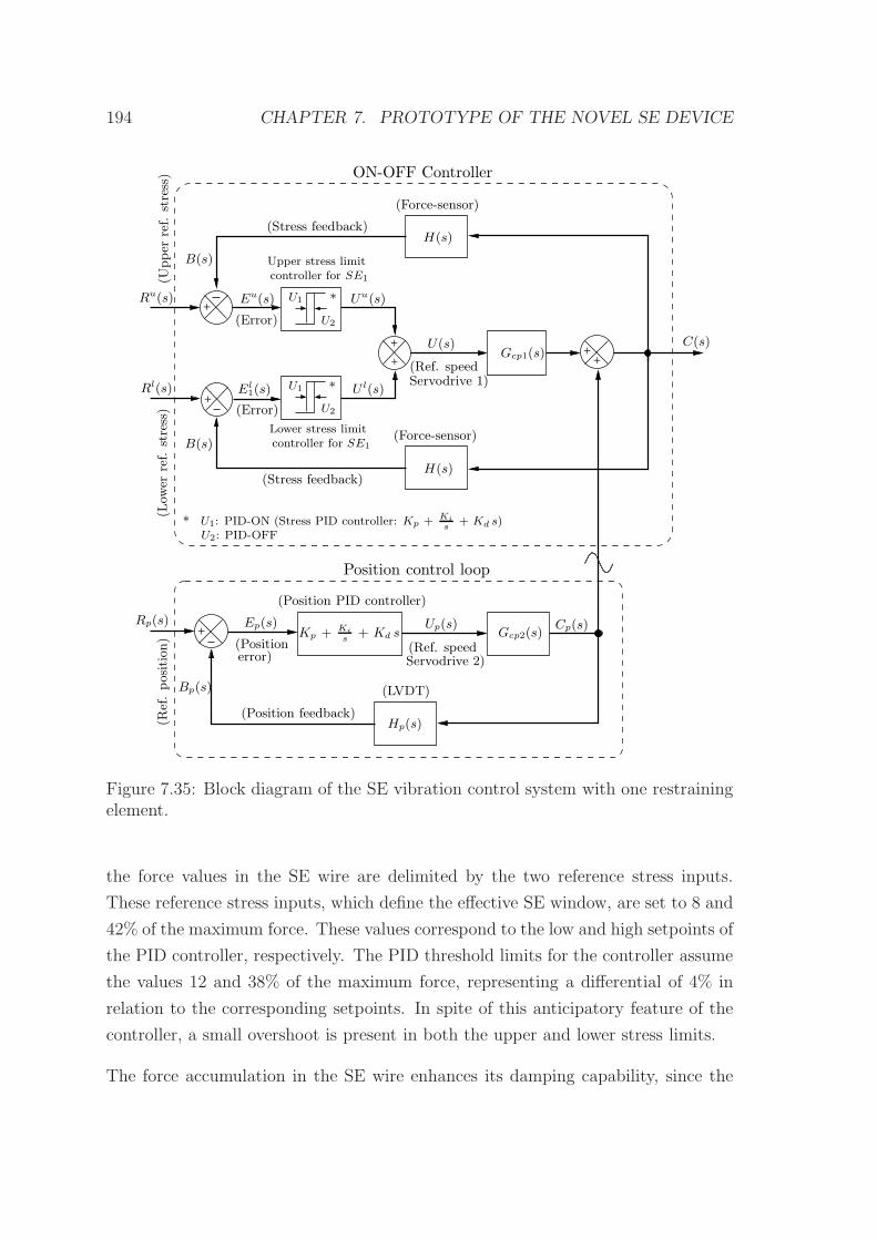
194 CHAPTER 7. PROTOTYPE OF THE NOVEL SE DEVICE
+
++
+
+
+
+
U1
U2
U1
H(s)
(Force-sensor)
Upper stress limitcontroller for SE1
Lower stress limitcontroller for SE1
Gcp1(s)
H(s)
(Ref. speedServodrive 1)
U2: PID-OFFU1: PID-ON (Stress PID controller: Kp + Ki
s+ Kd s)∗
U2
El1(s)
Eu(s) Uu(s)
U l(s)∗
C(s)U(s)
(Stress feedback)
(Stress feedback)
(Upper
ref.
stress)
Rl(s)
(Low
erref.
stress)
(Error)
(Error)
∗Ru(s)
B(s)
B(s)
(Force-sensor)
Position control loop
(Position PID controller)
(Positionerror)
Hp(s)
(Ref. speed
(LVDT)
Rp(s)
Servodrive 2)
Gcp2(s)
(Position feedback)
Up(s) Cp(s)Ep(s)
ON-OFF Controller(R
ef.position)
Bp(s)
Kp + Ki
s+ Kd s
Figure 7.35: Block diagram of the SE vibration control system with one restrainingelement.
the force values in the SE wire are delimited by the two reference stress inputs.
These reference stress inputs, which define the effective SE window, are set to 8 and
42% of the maximum force. These values correspond to the low and high setpoints of
the PID controller, respectively. The PID threshold limits for the controller assume
the values 12 and 38% of the maximum force, representing a differential of 4% in
relation to the corresponding setpoints. In spite of this anticipatory feature of the
controller, a small overshoot is present in both the upper and lower stress limits.
The force accumulation in the SE wire enhances its damping capability, since the
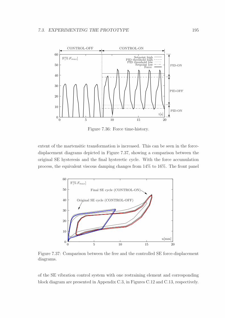
7.3. EXPERIMENTING THE PROTOTYPE 195
10
00 5 10 15 20
50
40
30
20
60
PID-ON
PID-OFF
PID-ON
t[s]
Setpoint highPID threshold highPID threshold low
Setpoint lowForce
F[%Fmax]
CONTROL-ONCONTROL-OFF
Figure 7.36: Force time-history.
extent of the martensitic transformation is increased. This can be seen in the force-
displacement diagrams depicted in Figure 7.37, showing a comparison between the
original SE hysteresis and the final hysteretic cycle. With the force accumulation
process, the equivalent viscous damping changes from 14% to 16%. The front panel
10
00
50
40
60
30
20
20105 15
F[%Fmax]
u[mm]
Original SE cycle (CONTROL-OFF)
Final SE cycle (CONTROL-ON)
Figure 7.37: Comparison between the free and the controlled SE force-displacementdiagrams.
of the SE vibration control system with one restraining element and corresponding
block diagram are presented in Appendix C.3, in Figures C.12 and C.13, respectively.
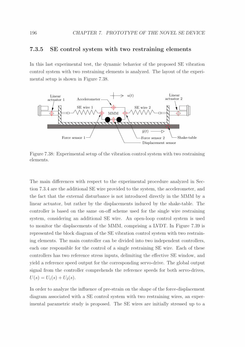
196 CHAPTER 7. PROTOTYPE OF THE NOVEL SE DEVICE
7.3.5 SE control system with two restraining elements
In this last experimental test, the dynamic behavior of the proposed SE vibration
control system with two restraining elements is analyzed. The layout of the experi-
mental setup is shown in Figure 7.38.
actuator 2Linear
actuator 1Linear
y(t)
u(t)
MMM
SE wire 1 SE wire 2
Force sensor 1 Force sensor 2
Displacement sensor
Shake-table
Accelerometer
Figure 7.38: Experimental setup of the vibration control system with two restrainingelements.
The main differences with respect to the experimental procedure analyzed in Sec-
tion 7.3.4 are the additional SE wire provided to the system, the accelerometer, and
the fact that the external disturbance is not introduced directly in the MMM by a
linear actuator, but rather by the displacements induced by the shake-table. The
controller is based on the same on-off scheme used for the single wire restraining
system, considering an additional SE wire. An open-loop control system is used
to monitor the displacements of the MMM, comprising a LVDT. In Figure 7.39 is
represented the block diagram of the SE vibration control system with two restrain-
ing elements. The main controller can be divided into two independent controllers,
each one responsible for the control of a single restraining SE wire. Each of these
controllers has two reference stress inputs, delimiting the effective SE window, and
yield a reference speed output for the corresponding servo-drive. The global output
signal from the controller comprehends the reference speeds for both servo-drives,
U(s) = U1(s) + U2(s).
In order to analyze the influence of pre-strain on the shape of the force-displacement
diagram associated with a SE control system with two restraining wires, an exper-
imental parametric study is proposed. The SE wires are initially stressed up to a
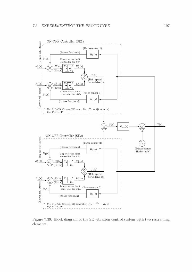
7.3. EXPERIMENTING THE PROTOTYPE 197
+
++
+
+
+
+
+
+
+
+
+
Gcp(s)
U1
U2
U1
U1
U2
U1
Upper stress limitcontroller for SE1
Lower stress limitcontroller for SE1
(Ref. speedServodrive 1)
(Ref. speedServodrive 2)
Upper stress limitcontroller for SE2
Lower stress limitcontroller for SE2
(Force-sensor 1)
(Force-sensor 2)
(Force-sensor 2)
(Force-sensor 1)
U2: PID-OFFU1: PID-ON (Stress PID controller: Kp +
Kis
+ Kd s)∗
U2: PID-OFFU1: PID-ON (Stress PID controller: Kp +
Kis
+ Kd s)∗
(Disturbance:Shake-table)
C(s)
U2
∗
(Stress feedback)
(Stress feedback)
(Upper
ref.
stress)
(Low
erref.
stress)
(Error)
(Error)
∗
U2
∗
(Stress feedback)
(Stress feedback)
(Upper
ref.
stress)
(Low
erref.
stress)
(Error)
(Error)
∗
H2(s)
H2(s)
H1(s)
H1(s)
U1(s)
U2(s)
Uu1 (s)
U l1(s)
Uu2 (s)
U l2(s)
Eu2 (s)
El2(s)
Eu1 (s)
El1(s)
B1(s)
B1(s)
B2(s)
B2(s)
ON-OFF Controller (SE1)
ON-OFF Controller (SE2)
Ru1 (s)
Rl1(s)
Ru2 (s)
Rl2(s)
U(s)
Figure 7.39: Block diagram of the SE vibration control system with two restrainingelements.
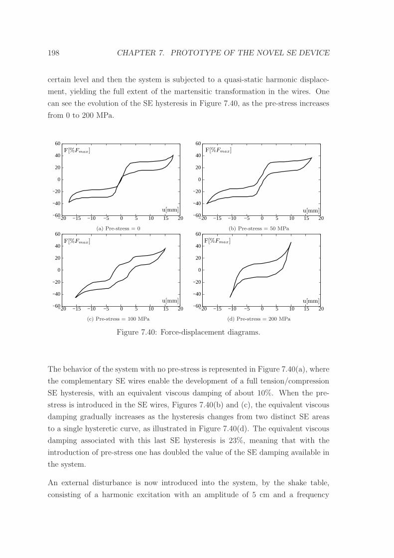
198 CHAPTER 7. PROTOTYPE OF THE NOVEL SE DEVICE
certain level and then the system is subjected to a quasi-static harmonic displace-
ment, yielding the full extent of the martensitic transformation in the wires. One
can see the evolution of the SE hysteresis in Figure 7.40, as the pre-stress increases
from 0 to 200 MPa.
60
40
20
0
−20
−40
−60−20 −15 −10 −5 0 5 10 15 20
F[%Fmax]
u[mm]
(a) Pre-stress = 0
60
40
20
0
−20
−40
−60−20 −15 −10 −5 0 5 10 15 20
F[%Fmax]
u[mm]
(b) Pre-stress = 50 MPa 60
40
20
0
−20
−40
−60−20 −15 −10 −5 0 5 10 15 20
F[%Fmax]
u[mm]
(c) Pre-stress = 100 MPa
60
40
20
0
−20
−40
−60−20 −15 −10 −5 0 5 10 15 20
F[%Fmax]
u[mm]
(d) Pre-stress = 200 MPa
Figure 7.40: Force-displacement diagrams.
The behavior of the system with no pre-stress is represented in Figure 7.40(a), where
the complementary SE wires enable the development of a full tension/compression
SE hysteresis, with an equivalent viscous damping of about 10%. When the pre-
stress is introduced in the SE wires, Figures 7.40(b) and (c), the equivalent viscous
damping gradually increases as the hysteresis changes from two distinct SE areas
to a single hysteretic curve, as illustrated in Figure 7.40(d). The equivalent viscous
damping associated with this last SE hysteresis is 23%, meaning that with the
introduction of pre-stress one has doubled the value of the SE damping available in
the system.
An external disturbance is now introduced into the system, by the shake table,
consisting of a harmonic excitation with an amplitude of 5 cm and a frequency
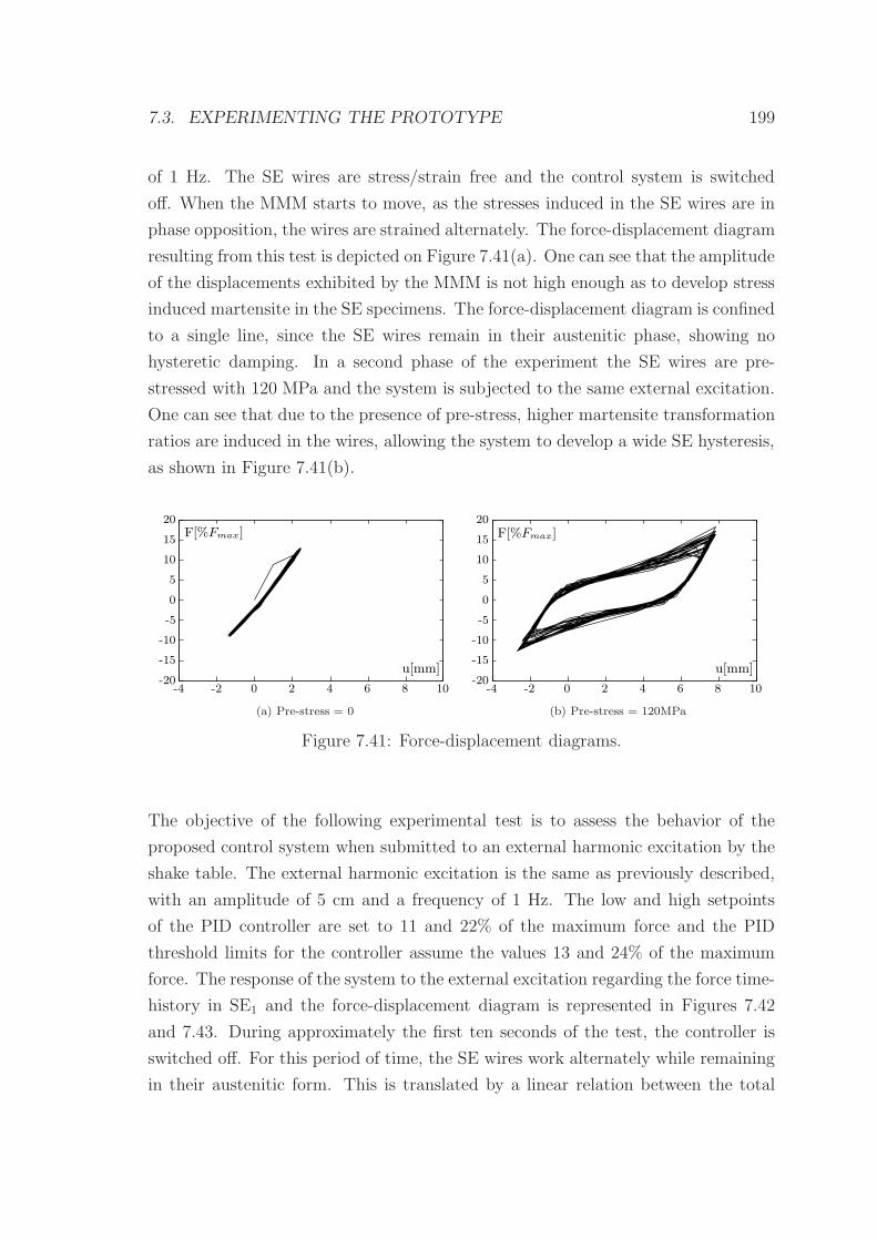
7.3. EXPERIMENTING THE PROTOTYPE 199
of 1 Hz. The SE wires are stress/strain free and the control system is switched
off. When the MMM starts to move, as the stresses induced in the SE wires are in
phase opposition, the wires are strained alternately. The force-displacement diagram
resulting from this test is depicted on Figure 7.41(a). One can see that the amplitude
of the displacements exhibited by the MMM is not high enough as to develop stress
induced martensite in the SE specimens. The force-displacement diagram is confined
to a single line, since the SE wires remain in their austenitic phase, showing no
hysteretic damping. In a second phase of the experiment the SE wires are pre-
stressed with 120 MPa and the system is subjected to the same external excitation.
One can see that due to the presence of pre-stress, higher martensite transformation
ratios are induced in the wires, allowing the system to develop a wide SE hysteresis,
as shown in Figure 7.41(b).
20
15
10
5
0
-5
-10
-15
-20-4 -2 0 2 4 6 8 10
F[%Fmax]
u[mm]
(a) Pre-stress = 0
20
15
10
5
0
-5
-10
-15
-20-4 -2 0 2 4 6 8 10
F[%Fmax]
u[mm]
(b) Pre-stress = 120MPa
Figure 7.41: Force-displacement diagrams.
The objective of the following experimental test is to assess the behavior of the
proposed control system when submitted to an external harmonic excitation by the
shake table. The external harmonic excitation is the same as previously described,
with an amplitude of 5 cm and a frequency of 1 Hz. The low and high setpoints
of the PID controller are set to 11 and 22% of the maximum force and the PID
threshold limits for the controller assume the values 13 and 24% of the maximum
force. The response of the system to the external excitation regarding the force time-
history in SE1 and the force-displacement diagram is represented in Figures 7.42
and 7.43. During approximately the first ten seconds of the test, the controller is
switched off. For this period of time, the SE wires work alternately while remaining
in their austenitic form. This is translated by a linear relation between the total
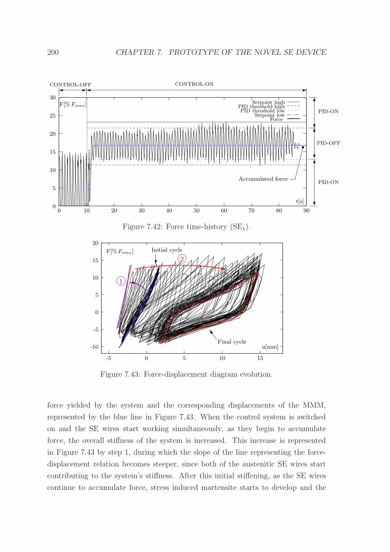
200 CHAPTER 7. PROTOTYPE OF THE NOVEL SE DEVICE
30
25
20
15
10
5
00 10 20 30 40 50 60 70 80 90
Setpoint highPID threshold highPID threshold low
Setpoint lowForce
Accumulated force
CONTROL-ONCONTROL-OFF
PID-ON
PID-OFF
PID-ON
F[%Fmax]
t[s]
Figure 7.42: Force time-history (SE1).
20
15
10
5
0
-5
-10
-5 0 5 10 15
1
2F[%Fmax] Initial cycle
Final cycleu[mm]
Figure 7.43: Force-displacement diagram evolution.
force yielded by the system and the corresponding displacements of the MMM,
represented by the blue line in Figure 7.43. When the control system is switched
on and the SE wires start working simultaneously, as they begin to accumulate
force, the overall stiffness of the system is increased. This increase is represented
in Figure 7.43 by step 1, during which the slope of the line representing the force-
displacement relation becomes steeper, since both of the austenitic SE wires start
contributing to the system’s stiffness. After this initial stiffening, as the SE wires
continue to accumulate force, stress induced martensite starts to develop and the
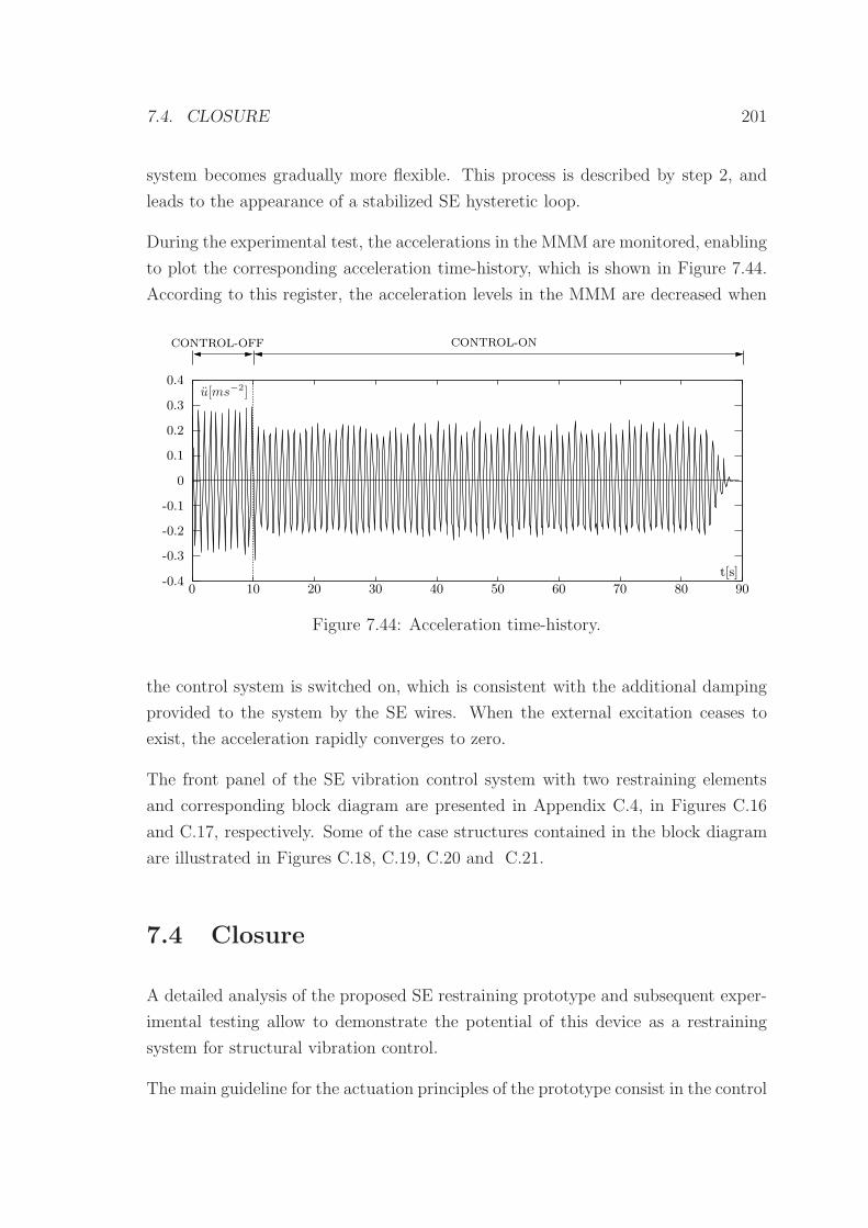
7.4. CLOSURE 201
system becomes gradually more flexible. This process is described by step 2, and
leads to the appearance of a stabilized SE hysteretic loop.
During the experimental test, the accelerations in the MMM are monitored, enabling
to plot the corresponding acceleration time-history, which is shown in Figure 7.44.
According to this register, the acceleration levels in the MMM are decreased when
0.4
0.3
0.2
0.1
0
-0.1
-0.2
-0.3
-0.40 10 20 30 40 50 60 70 80 90
CONTROL-OFF
u[ms−2]
t[s]
CONTROL-ON
Figure 7.44: Acceleration time-history.
the control system is switched on, which is consistent with the additional damping
provided to the system by the SE wires. When the external excitation ceases to
exist, the acceleration rapidly converges to zero.
The front panel of the SE vibration control system with two restraining elements
and corresponding block diagram are presented in Appendix C.4, in Figures C.16
and C.17, respectively. Some of the case structures contained in the block diagram
are illustrated in Figures C.18, C.19, C.20 and C.21.
7.4 Closure
A detailed analysis of the proposed SE restraining prototype and subsequent exper-
imental testing allow to demonstrate the potential of this device as a restraining
system for structural vibration control.
The main guideline for the actuation principles of the prototype consist in the control
202 CHAPTER 7. PROTOTYPE OF THE NOVEL SE DEVICE
of the stress level in the SE wires during the dynamic excitation, with the possibility
to accumulate stress, enabling higher martensite ratios, and to relieve stress, pre-
venting the wires from yielding. A thorough description of the kernel parts of the
prototype provide an extended insight into the developed approach to meet these
guidelines. The integration of the control algorithms into the prototype is also ad-
dressed. The control algorithms are implemented using a LabView platform, and
are based in a PID control approach. Several considerations regarding this type of
control systems are made, including relevant aspects related to the tuning of the
controller.
To accomplish the proposed objective, several experimental setups are tested. The
last experimental procedure features a fully operational version of the proposed SE
vibration control system with two restraining SE elements. The response of the
system to an external harmonic excitation, induced by a shake table, proves to be
rather adequate. The system promotes the force accumulation in the SE wires,
enabling the development of a wide SE hysteretic loop, while also controling their
maximum force and decreasing the acceleration of the MMM.
Chapter 8
Summary, Conclusions and Future
Work
8.1 Summary and conclusions
Shape-memory alloys are a class of peculiar metallic alloys presenting a unique prop-
erty regarding applications in structural vibration control: superelasticity. It derives
from a diffusionless phase transformation in solids called martensitic transformation.
This crystallographic phase transformation depends on stress and temperature and
enables the material to change from the parent phase, a high energy phase called
austenite to a low energy phase called martensite. Superelasticity is associated
with the formation of stress induced martensite, which is developed above a certain
critical stress threshold. It translates into the ability of the material to totally re-
cover from large, nonlinear, deformations while developing a hysteretic loop. This
superelastic hysteretic behavior confers to SMAs a vast potential for technological
applications in the field of seismic structural hazard mitigation.
One of the main objectives of this study has been the characterization of the behavior
of superelastic Nitinol, identifying ways to optimize its properties for seismic appli-
cations. An extensive experimental program is conducted, including temperature-
controlled cyclic tensile tests, differential scanning calorimetry and infrared thermo-
imaging. These experimental tests are complemented by an exhaustive analysis of
the corresponding phase-diagram paths and superelastic hysteresis, providing a valu-
203
204 CHAPTER 8. SUMMARY, CONCLUSIONS AND FUTURE WORK
able insight into the identification of the main variables influencing the superelastic
damping in Nitinol.
After discussing the theoretical background concerning constitutive models for SMAs,
a rate-independent model and a rate-dependent model are implemented. These
strain-driven, time-discrete numerical models couple the mechanical laws with the
kinetic transformation laws, and also with a heat balance equation describing the
convective heat problem, in the case of the rate-dependent model. The good per-
formance of these numerical models is confirmed by comparing the numerical sim-
ulations with experimental data and literature results from a series of strain-rate
analysis with frequency ranging from 0.2 to 4 Hz.
To illustrate the performance of superelastic wires when acting as restoring elements
in passive seismic control devices, numerical models of a couple of dynamic systems
are analyzed, including a simplified numerical model of a railway viaduct equipped
with a superelastic restraining system. This analysis confirms the benefits of using
SMAs in passive seismic control devices and encourages future investigations in the
field.
The most important contribution of this work consists on the development of an
original semi-active vibration control device, which is able to dissipate a considerable
amount of energy during a dynamic event, while keeping the superelastic wires inside
recoverable limits defined by a prescribed superelastic window. This limits the
degradation effects due to cyclic loading in SE Nitinol, also reducing the influence of
cycling on damping. With this device, strain accumulation in the SE Nitinol wires
derives from the the structural displacements during the dynamic action, avoiding
permanent pre-strain in the material with the associated stress-relaxation.
A small-scale prototype of this device is built, simulating the proposed SE vibration
control system, comprising two restraining superelastic elements.
The main findings resulting from this study include the following: The superelastic damping capacity of Nitinol is influenced by temperature.
An increase on ambient temperature, in strain-controlled situations, causes
the damping capacity of the Nitinol wires to marginally decrease. It is also
showed that an annual temperature variation of 20C, yields an increment on
the critical stress to induce martensite of about 130 MPa, compromising the
8.1. SUMMARY AND CONCLUSIONS 205
SIM development. Hence, an adequate temperature isolation system would
highly benefit a vibration mitigation device based on superelastic SMAs. The superelastic damping capacity of a Nitinol wire is influenced by strain-
amplitude. As the strain-amplitude increases, the damping capacity of SE
Nitinol also increases. The superelastic damping capacity of a Nitinol wire is influenced by strain-
rate. In fact, when passing from quasi-static loading conditions to dynamic
ones, important changes occur in the temperature time-history and in the
corresponding stress-strain diagram, affecting its dissipation capacity. The
evaluation of the equivalent viscous damping for a wide range of strain-rates
demonstrated that, as the strain-rate increased from quasi-static conditions,
the dissipation capacity of the Nitinol wire first suffers a slight increase and
then decreases until it stabilizes. The development of a rate-dependent nu-
merical model, coupling mechanical and kinetic transformations laws with a
thermal balance equation, allowed to apprehend the dynamic behavior of SE
Nitinol at higher strain-rates. This model confirmed that for a cyclic strain-
amplitude of 6.5%, the behavior of SE Nitinol wires is mainly insensitive to
strain-rate for frequencies in the range of 0.2 to 4 Hz. The superelastic damping capacity of a Nitinol wire is influenced by cyclic
loading. In fact, cyclic loading causes cumulative creep deformation in SE
Nitinol, increasing the elongation of the wire. For a given oscillation amplitude
this is translated in a decrease of the wire’s net strain, along with the amount
of dissipated energy. Cyclic loading also causes the decrease in both the critical
stress to induce martensite and in the width of the hysteretic loop. According
to the experimental tests, these effects can be rather important, amounting
up to 1.1% of accumulated strain, a maximum decrease of about 160 MPa in
the critical stress for SIM and an average strain decrease of 1.5% on the SE
hysteretic width. These effects gradually stabilize with cycling, although this
stabilization process can endure for about 100 cycles. During this process the
damping capacity of the SE Nitinol wire continuously decreases. It was also
shown that the degradation increases with both temperature and strain-rate. The superelastic damping capacity of a Nitinol wire is influenced by aging at
constant strain in the coexistence zone. It is shown that if the material ages at
206 CHAPTER 8. SUMMARY, CONCLUSIONS AND FUTURE WORK
constant strain in the coexistence domain, a stress step occurs, leading to the
stress relaxation of the material. As pre-strain is very important in superelastic
based vibration control devices, because it enhances their damping capacity,
the stress relaxation of the material has to be conveniently controlled. The performance of several SDOF mechanisms based on SE restoring elements
is analyzed under dynamic loading, emphasizing their capability to mitigate
vibrations and self-centering abilities. The great versatility of SMA devices
is confirmed, being able to describe a wide variety of cyclic behaviors, from
fully re-centering to highly dissipating. This can be achieved by making simple
functional variations of the SMA components and by acting on their mechani-
cal properties. The shape of the hysteretic loops can be adjusted for a specific
application, according to its particular dynamic requirements. One of these
devices is successfully tested as a seismic passive vibration control system in
a simplified numerical model of a railway viaduct. This analysis confirmed
the potential of SMAs in passive seismic control devices and encourages future
investigations in the field. A detailed analysis of the proposed superelastic restraining prototype allows to
demonstrate the potential of this device as a restraining system for structural
vibration control. The guidelines for the actuation principles of the prototype
mainly consist in the control of the stress level in the superelastic wires, during
the dynamic excitation, with the possibility to accumulate stress and enable
higher martensite ratios. A thorough description of the kernel parts of the
prototype enables an extended insight into the developed approach to meet
these guidelines. The integration of the control algorithms into the prototype
is also addressed. The control algorithms are implemented using a LabView
platform, and are based in a PID control approach. Several considerations
regarding this type of control systems are made, including relevant aspects
related to the tuning of the controller. To accomplish the proposed objective
several experimental setups are considered. The last experimental procedure
features a full operational prototype of the proposed SE vibration control
system with two restraining superelastic elements.
8.2. FUTURE WORK 207
8.2 Future Work
This work has presented a full operational prototype of a SE vibration control de-
vice, being able to adequately fulfill a series of prescribed stress control guidelines.
However, even though the implementation of these guidelines yielded a successful
vibration control mechanism, mainly for academic pursuits, there are several aspects
in which this mechanism can be further improved through additional research.
The main drawback of the presented mechanism consists in the fact that the stress
control in the SE Nitinol wires is achieved through the use of electromechanical
actuators. The compensation either for high or low stresses in the SE wires is
achieved by the movement of these actuators, which are placed in series with the
wires, in the force flow path. This means that the actuators have to be able to sustain
the forces developed in the SE wires during the dynamic loading, which, in the
case of civil engineering structures, are considerable high. In order to comply with
these forces it would be necessary to use high bearing capacity electromechanical
actuators, with high costs and high energy demands, undesirable to a restraining
mechanism. In order to meet the requirements of fast response and low power
consumption, promising alternatives are being currently studied.
In what follows, a general description of these alternative stress control mechanisms
is presented: To compensate for low stresses the SE Nitinol wire is connected to a retractor
by a webbing. This retractor uses a spool as its central element, which is at-
tached to the other end of the webbing. Inside the retractor an angular spring
applies a force to the spool, so it winds up any loose wire. When the wire is
pulled out due to slow structural deformations associated with ambient tem-
perature variations or rheological effects, the spool rotates counter-clockwise,
turning the attached spring in the same direction. In fact, the rotating spool
works to untwist the spring. As the spring wants to return to its original
shape, it resists this twisting motion. If the SE Nitinol wire is released, the
spring tightens up, rotating the spool clockwise until there is no more slack
in the wire. The retractor also has a locking mechanism that stops the spool
from rotating when the structure undergoes a fast dynamic action. This may
be implemented by a weighted pendulum or a ball bearing that are deflected
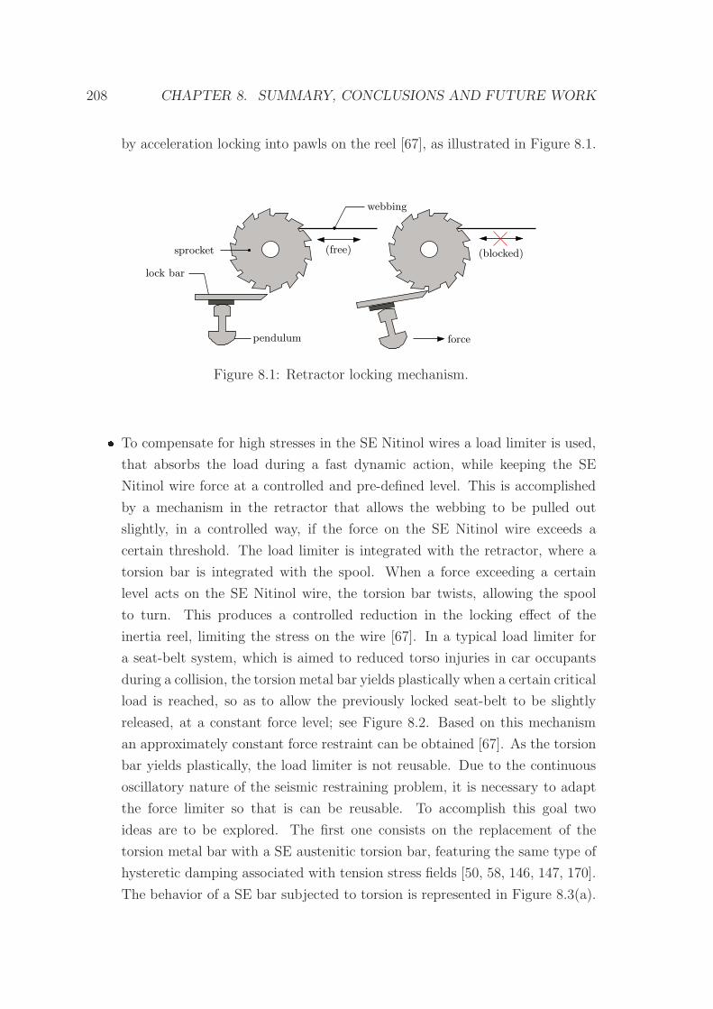
208 CHAPTER 8. SUMMARY, CONCLUSIONS AND FUTURE WORK
by acceleration locking into pawls on the reel [67], as illustrated in Figure 8.1.
sprocket
lock bar
pendulum
(free)
webbing
force
(blocked)
Figure 8.1: Retractor locking mechanism. To compensate for high stresses in the SE Nitinol wires a load limiter is used,
that absorbs the load during a fast dynamic action, while keeping the SE
Nitinol wire force at a controlled and pre-defined level. This is accomplished
by a mechanism in the retractor that allows the webbing to be pulled out
slightly, in a controlled way, if the force on the SE Nitinol wire exceeds a
certain threshold. The load limiter is integrated with the retractor, where a
torsion bar is integrated with the spool. When a force exceeding a certain
level acts on the SE Nitinol wire, the torsion bar twists, allowing the spool
to turn. This produces a controlled reduction in the locking effect of the
inertia reel, limiting the stress on the wire [67]. In a typical load limiter for
a seat-belt system, which is aimed to reduced torso injuries in car occupants
during a collision, the torsion metal bar yields plastically when a certain critical
load is reached, so as to allow the previously locked seat-belt to be slightly
released, at a constant force level; see Figure 8.2. Based on this mechanism
an approximately constant force restraint can be obtained [67]. As the torsion
bar yields plastically, the load limiter is not reusable. Due to the continuous
oscillatory nature of the seismic restraining problem, it is necessary to adapt
the force limiter so that is can be reusable. To accomplish this goal two
ideas are to be explored. The first one consists on the replacement of the
torsion metal bar with a SE austenitic torsion bar, featuring the same type of
hysteretic damping associated with tension stress fields [50, 58, 146, 147, 170].
The behavior of a SE bar subjected to torsion is represented in Figure 8.3(a).
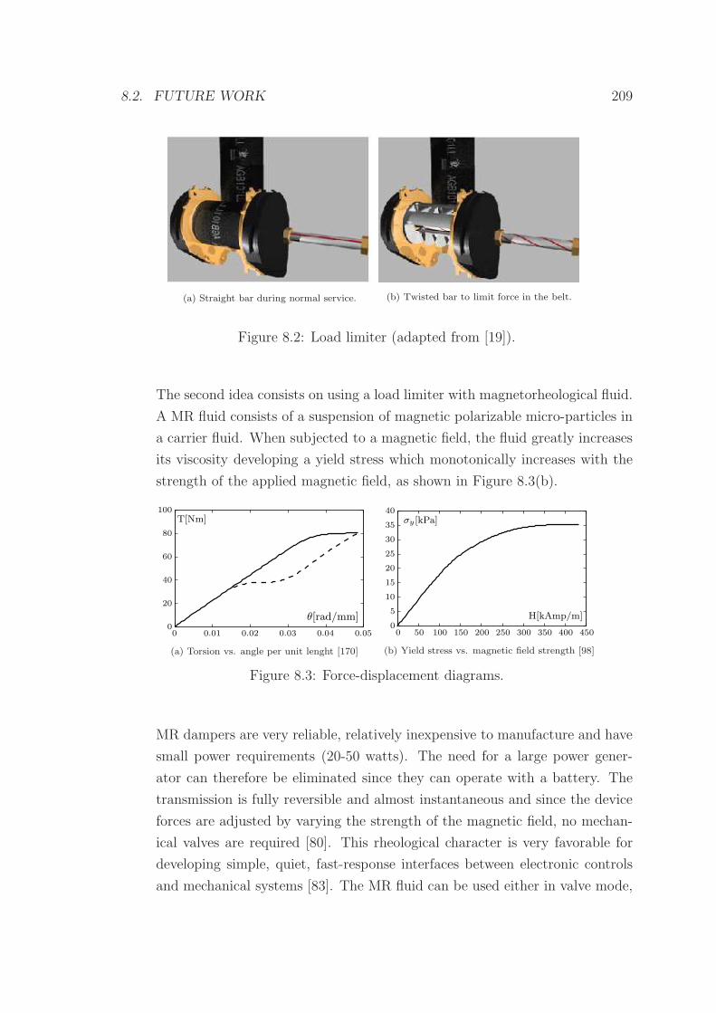
8.2. FUTURE WORK 209
(a) Straight bar during normal service. (b) Twisted bar to limit force in the belt.
Figure 8.2: Load limiter (adapted from [19]).
The second idea consists on using a load limiter with magnetorheological fluid.
A MR fluid consists of a suspension of magnetic polarizable micro-particles in
a carrier fluid. When subjected to a magnetic field, the fluid greatly increases
its viscosity developing a yield stress which monotonically increases with the
strength of the applied magnetic field, as shown in Figure 8.3(b).
0.010 0.02 0.03 0.04 0.05
100
80
60
40
20
0θ[rad/mm]
T[Nm]
(a) Torsion vs. angle per unit lenght [170]
0 50 100 150 200 250 300 350 400 450
40
35
30
25
20
15
10
5
0H[kAmp/m]
σy [kPa]
(b) Yield stress vs. magnetic field strength [98]
Figure 8.3: Force-displacement diagrams.
MR dampers are very reliable, relatively inexpensive to manufacture and have
small power requirements (20-50 watts). The need for a large power gener-
ator can therefore be eliminated since they can operate with a battery. The
transmission is fully reversible and almost instantaneous and since the device
forces are adjusted by varying the strength of the magnetic field, no mechan-
ical valves are required [80]. This rheological character is very favorable for
developing simple, quiet, fast-response interfaces between electronic controls
and mechanical systems [83]. The MR fluid can be used either in valve mode,
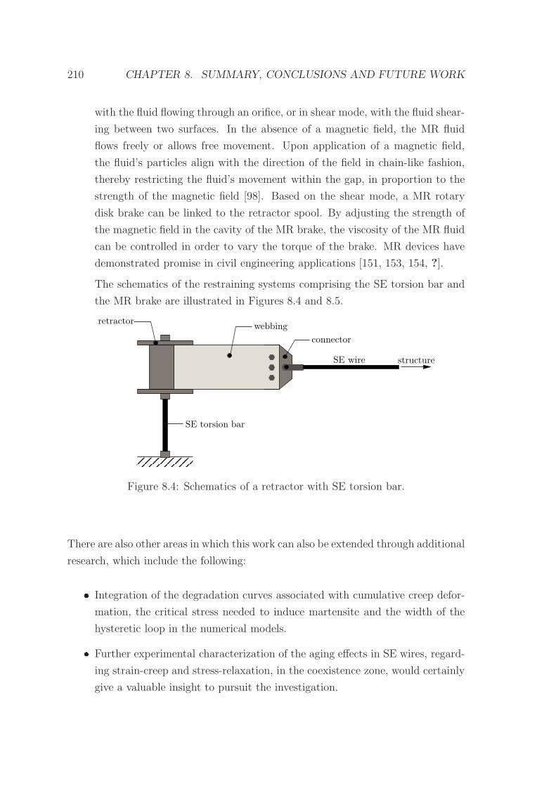
210 CHAPTER 8. SUMMARY, CONCLUSIONS AND FUTURE WORK
with the fluid flowing through an orifice, or in shear mode, with the fluid shear-
ing between two surfaces. In the absence of a magnetic field, the MR fluid
flows freely or allows free movement. Upon application of a magnetic field,
the fluid’s particles align with the direction of the field in chain-like fashion,
thereby restricting the fluid’s movement within the gap, in proportion to the
strength of the magnetic field [98]. Based on the shear mode, a MR rotary
disk brake can be linked to the retractor spool. By adjusting the strength of
the magnetic field in the cavity of the MR brake, the viscosity of the MR fluid
can be controlled in order to vary the torque of the brake. MR devices have
demonstrated promise in civil engineering applications [151, 153, 154, ?].
The schematics of the restraining systems comprising the SE torsion bar and
the MR brake are illustrated in Figures 8.4 and 8.5.
retractorwebbing
connector
SE wire structure
SE torsion bar
Figure 8.4: Schematics of a retractor with SE torsion bar.
There are also other areas in which this work can also be extended through additional
research, which include the following: Integration of the degradation curves associated with cumulative creep defor-
mation, the critical stress needed to induce martensite and the width of the
hysteretic loop in the numerical models. Further experimental characterization of the aging effects in SE wires, regard-
ing strain-creep and stress-relaxation, in the coexistence zone, would certainly
give a valuable insight to pursuit the investigation.
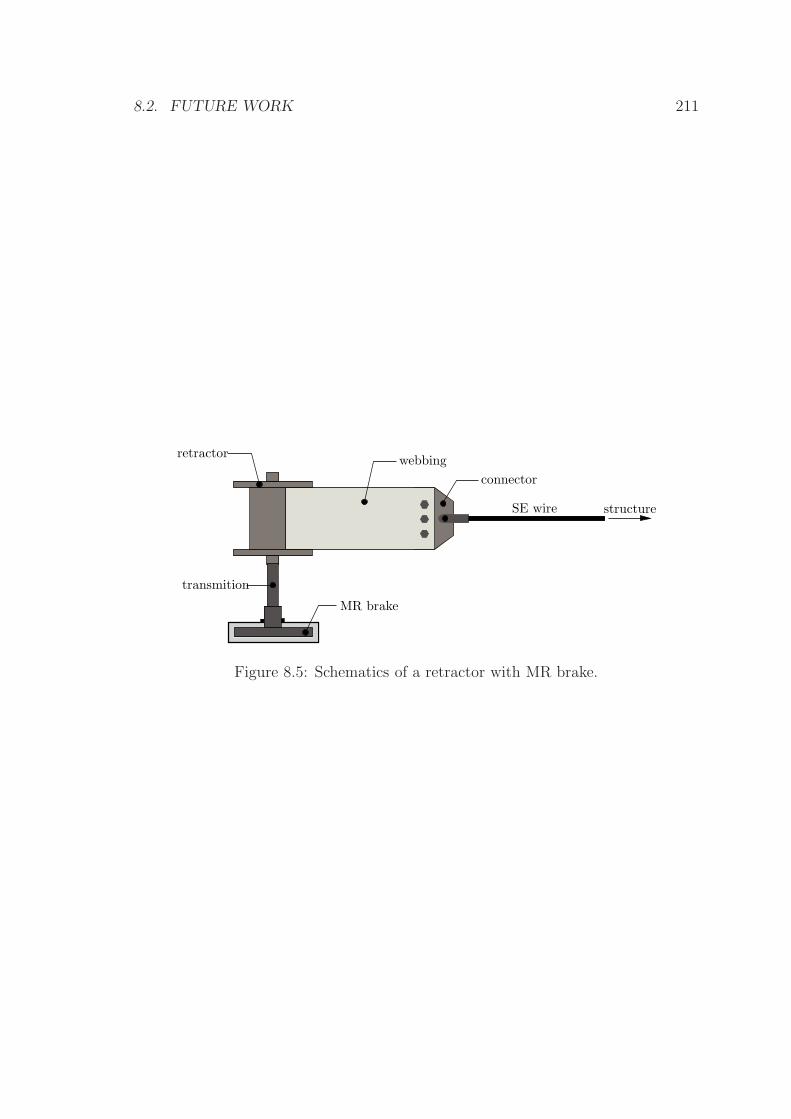
8.2. FUTURE WORK 211
retractorwebbing
connector
MR brake
SE wire structure
transmition
Figure 8.5: Schematics of a retractor with MR brake.

212 CHAPTER 8. SUMMARY, CONCLUSIONS AND FUTURE WORK
Appendix A
Modeling of control systems
In this appendix are presented some introductory concepts regarding the modeling
of control systems.
A.1 Laplace Transformation
A.1.1 Definition of the Laplace transformation
The Laplace transform of a function f(t), defined for all real numbers t ≥ 0, is the
function F (s), defined by [92]:
F (s) = L [(f(t)] =
∫
∞
0
e−stdt[f(t)] =
∫
∞
0
f(t) e−stdt (A.1)
where s is a complex variable and L is an operator indicating that the quantity
that it prefixes is to be transformed by the Laplace integral∫
∞
0e−stdt.
For the Laplace transform of a function f(t) to exist, the Laplace integral has to
converge. The integral will converge if f(t) is piecewise continue in every finite
interval for t > 0 and if it is of exponential order as t approaches infinity. The
function f(t) has an exponential order at infinity if, and only if, there exist α and
M such that
|f(t)| ≤Me−α t
213
214 APPENDIX A. MODELING OF CONTROL SYSTEMS
Then, the Laplace transform L [(f(t)] is defined for s > α.
A.1.2 Laplace transforms of several common functions
A.1.2.1 Step function
Consider the step function represented in Figure A.1, in which
f(t) =
0, for t < 0
A, for t > 0
where A is a constant.
f(t)
0
A
t
Figure A.1: Step function
The step function is not defined at t = 0. The Laplace transform of this step function
is calculated using the definition expressed in equation (A.1), yielding
F (s) = L [(f(t)] =
∫
∞
0
f(t) e−stdt =
∫
∞
0
Ae−stdt =
= −Ae−st
s
∣
∣
∣
∞
0=A
s(A.2)
The step function in which A = 1 is called unit-step function or Heaviside step
function. The Laplace transform of the unit-step function is 1/s.
A.1. LAPLACE TRANSFORMATION 215
A.1.2.2 Ramp function
Consider the ramp function represented in Figure A.2, in which
f(t) =
0, for t < 0
A t, for t ≥ 0
where A is a constant.
1A
f(t)
0 t
Figure A.2: Ramp function
The Laplace transform of this ramp function is obtained as
F (s) = L [(f(t)] =
∫
∞
0
f(t) e−stdt =
∫
∞
0
At e−stdt =
=Ate−st
−s
∣
∣
∣
∞
0−
∫
∞
0
Ae−st
−se−stdt =
A
s2(A.3)
As in the case of the step function, the ramp function in which A = 1 is called
unit-ramp function.
216 APPENDIX A. MODELING OF CONTROL SYSTEMS
A.1.2.3 Pulse function
Consider the pulse function represented in Figure A.3, in which
f(t) =
A
t0, for t < 0 < t0
0 for t < 0, t0 < t
where A and t0 are constants.
f(t)
0 tt0
At0
Figure A.3: Pulse function
The Laplace transform of this pulse function is obtained as
F (s) = L [(f(t)] =
∫ t0
0
f(t) e−stdt =
∫ t0
0
A
t0e−stdt =
= −Ae−st
t0s
∣
∣
∣
t0
0=
A
t0s(1− e−st0) (A.4)
A.1.2.4 Impulse function
The impulse function is a special limiting case of the pulse function in which t0
tends to zero. It represents an infinitely sharp peak that bounds an area A, since
the height of the impulse is A/t0 and its duration is t0. This function has the value
zero everywhere except at x = 0 where its value is infinitely large, in such a way that
its total integral yields A. The schematic representation of the impulse function is
usually a line surmounted by an arrow, with the the value of the area A next to the
arrowhead, as shown in Figure A.4.
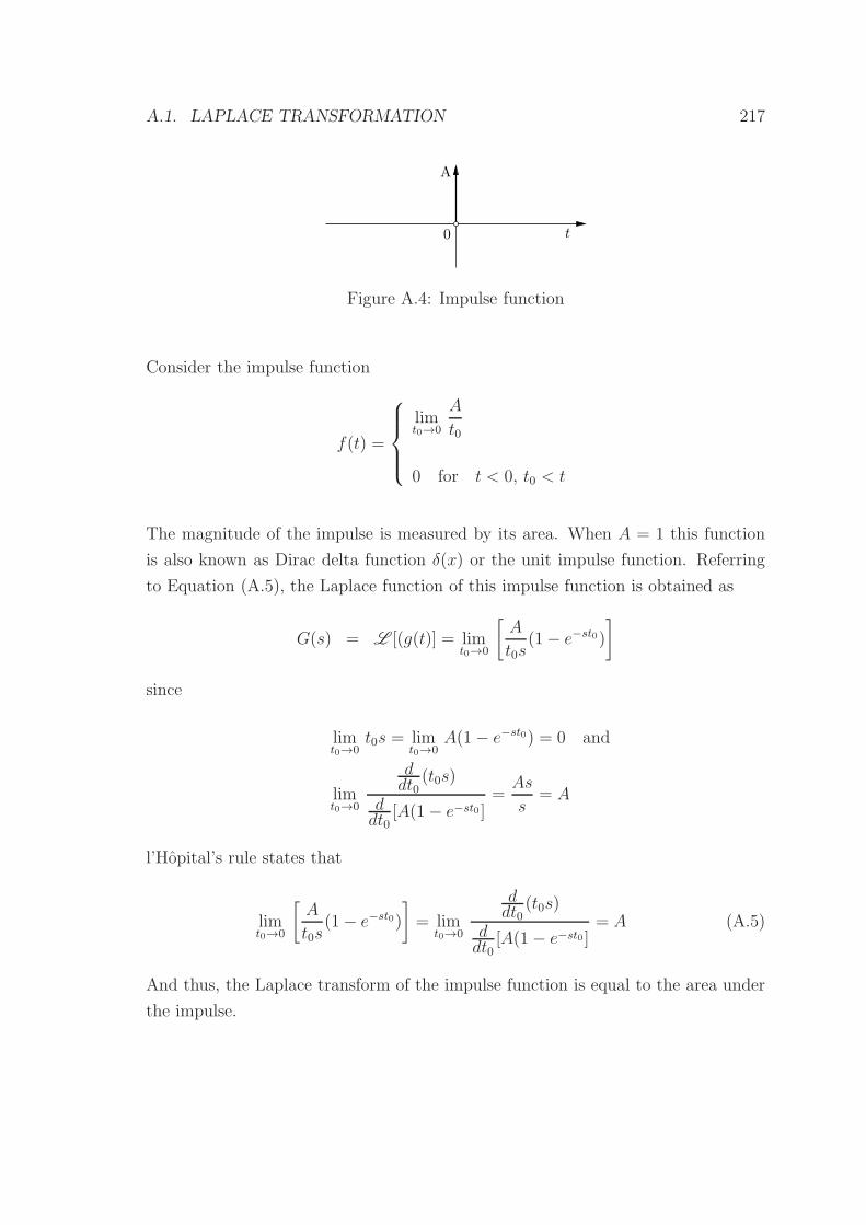
A.1. LAPLACE TRANSFORMATION 217
0
A
t
Figure A.4: Impulse function
Consider the impulse function
f(t) =
limt0→0
A
t0
0 for t < 0, t0 < t
The magnitude of the impulse is measured by its area. When A = 1 this function
is also known as Dirac delta function δ(x) or the unit impulse function. Referring
to Equation (A.5), the Laplace function of this impulse function is obtained as
G(s) = L [(g(t)] = limt0→0
[
A
t0s(1− e−st0)
]
since
limt0→0
t0s = limt0→0
A(1− e−st0) = 0 and
limt0→0
ddt0
(t0s)
ddt0
[A(1− e−st0 ]=As
s= A
l’Hopital’s rule states that
limt0→0
[
A
t0s(1− e−st0)
]
= limt0→0
ddt0
(t0s)
ddt0
[A(1− e−st0 ]= A (A.5)
And thus, the Laplace transform of the impulse function is equal to the area under
the impulse.
218 APPENDIX A. MODELING OF CONTROL SYSTEMS
A.1.3 Laplace transforms properties
A.1.3.1 Linearity
A linear function f(x) is a function that satisfies both the adaptivity and homogene-
ity properties. Additivity is also referred to as the superposition property and it
states that, the net response caused by two or more different forcing functions is the
sum of the responses which would have been caused by each forcing function indi-
vidually. This property can be mathematically expressed as f(x+ y) = f(x)+ f(y).
Homogeneity of degree 1 is when f(αx) = αf(x), for all α.
The Laplace transform is a linear function, and hence, the Laplace transform of a
sum is the sum of Laplace transforms of each term. Consider two Laplace trans-
formable functions f(t) and g(t) with Laplace transforms F (s) and G(s), respec-
tively.
L [f(t) + g(t)] = L [f(t)] + L [g(t)] = F (s) +G(s) (A.6)
This can be easily proved using basic rules of integration, as shown next
L [(f(t) + g(t)] =
∫
∞
0
[f(t) + g(t)] e−stdt =
=
∫
∞
0
f(t) e−stdt+
∫
∞
0
g(t) e−stdt = F (s) +G(s)
The homogeneity of the Laplace transform can be proved in the following way
L [af(t)] = aL [f(t)] = aF (s) (A.7)
L [a(f(t)] =
∫
∞
0
af(t) e−stdt =
= a
∫
∞
0
f(t) e−stdt = aF (s)
A.1. LAPLACE TRANSFORMATION 219
A.1.3.2 Differentiation and integration
Consider the Laplace integral expressed in Equation A.1. Integrating this integral
by parts yields
F (s) =
∫
∞
0
f(t)e−st dt = f(t)e−st
−s
∣
∣
∣
∞
0−
∫
∞
0
[
d
dtf(t)
]
e−st
−s=
=f(0)
s+
1
s
∫
∞
0
[
d
dtf(t)
]
e−st dt =f(0)
s+
1
sL
[
d
dtf(t)
]
this means that
L
[
d
dtf(t)
]
= sF (s)− f(0) (A.8)
where f(0) represents the value of f(t) evaluated at t = 0. This procedure may be
equally applied to the second derivative of f(t), yielding
L
[
d2
dt2f(t)
]
= s2F (s)− sf(0)− ˙f(0) (A.9)
where ˙f(0) represents the value of df(t)/dt evaluated at t = 0. In the case of the
nth derivative, one obtains
L
[
dn
dtnf(t)
]
= snF (s)− sn−1f(0)− sn−2 ˙f(0)− · · · − sf (n−2)(0)− f (n−1)(0)
where f(0), ˙f(0), . . . , f (n−1)(0) represent the values of f(t), df(t)/dt, . . . , d(n−1)/dt(n−1),
respectively evaluated at t = 0. If all the initial values of f(t) and its derivatives
are equal to zero, then the Laplace transform of the nth derivative of f(t) is given
by snF (s).
In order to obtain the Laplace transform of integrals one has to refer to Equa-
tion (A.1) and expand it using the integration by parts rules. This means that
L
[∫
f(t) dt
]
=
∫
∞
0
[∫
f(t) dt
]
e−stdt =
=
∫
f(t) dte−st
−s
∣
∣
∣
∞
0−
∫
∞
0
f(t)e−st
−sdt =
f−1(0)
s+F (s)
s(A.10)
where f−1(0) represents∫
f(t)dt at t = 0.
220 APPENDIX A. MODELING OF CONTROL SYSTEMS
In the case of a definite integral,∫ t
0f(t) dt, as
∫ t
0
f(t) dt =
∫
f(t) dt− f−1(0)
and
L
[∫ t
0
f(t) dt
]
= L
[∫
f(t) dt
]
− L[
f−1(0)]
since
L[
f−1(0)]
=f−1(0)
s
one obtains that
L
[∫ t
0
f(t) dt
]
=F (s)
s(A.11)
A.2 Transfer function
A transfer function is a mathematical representation of the relation between the
input and output of a linear, time-invariant (LTI) system. A system is called linear
if the relation between the input and the output of the system is a linear function.
Time invariance means that if an input is applied to a system, at any given time
instant, or τ seconds apart from that instant, the output will be identical, except
for the corresponding time delay. That is, if the output due to input x(t) is y(t),
then the output due to input x(t−τ) is y(t−τ). Hence, the system is time invariant
because the output does not depend on the particular time the input is applied.
Consider the LTI system defined by the following differential equation:
a0yn(t) + a1y
(n−1)(t) + · · ·+ a(n−1)y(t) + any(t) =
b0um(t) + b1u
(m−1)(t) + · · ·+ b(m−1)x(t) + bmx(t) (n ≥ m) (A.12)
where y(t) is the output variable of the system and x(t) is the input. Taking the
Laplace transforms of both sides of Equation A.12, and assuming that all initial
A.3. CONTROL SYSTEMS 221
conditions are zero, one obtains
(a0sn + a1s
(n−1) + · · ·+ a(n−1)s+ an)Y (s) =
= (b0sm + b1s
(m−1) + · · ·+ b(m−1)s+ bm)U(s)
The transfer function G(s), relating the input and output of a LTI system, yields
G(s) =Y (s)
U(s)=b0s
m + b1s(m−1) + · · ·+ b(m−1)s+ bm
a0sn + a1s(n−1) + · · ·+ a(n−1)s+ an
The order of the system is given by the highest power of s in the denominator of
the transfer function.
A.3 Control systems
The main objective of a automatic control system is to control a system variable,
causing it to comply with a desired reference value. This variable is measured and
controlled and it is called the controlled variable. Normally, the controlled variable
constitutes the output of the system. The manipulation of the controlled variable is
achieved by the system components through the variation, in a prescribed manner,
of the actuating signal, also called the input signal.
The basic control system concept may be graphically described by the simple block
diagram presented in Figure A.5, in which a system G, with a Laplace transfer func-
tion G(s), relates the input and the output signals. Block diagrams illustrate the
functions performed by each component of the control system, as well the correspon-
dent signal flows. Block diagrams are built up of functional blocks, which represent
the mathematical operation performed on the input signal, producing an output.
Transfer functions of the components are placed is the corresponding blocks, which
are connected by arrows to indicate the direction of the signals flow.
In this case, the output of the block O(s) is obtained by multiplying the input signal
I(s) by the transfer function G(s), i.e. O(s) = G(s)I(s), with G(s) = O(s)/I(s).
A summing operation can also be translated into a block diagram, by the use of a
circle where the various input signals converge, and an output signal emerges. To
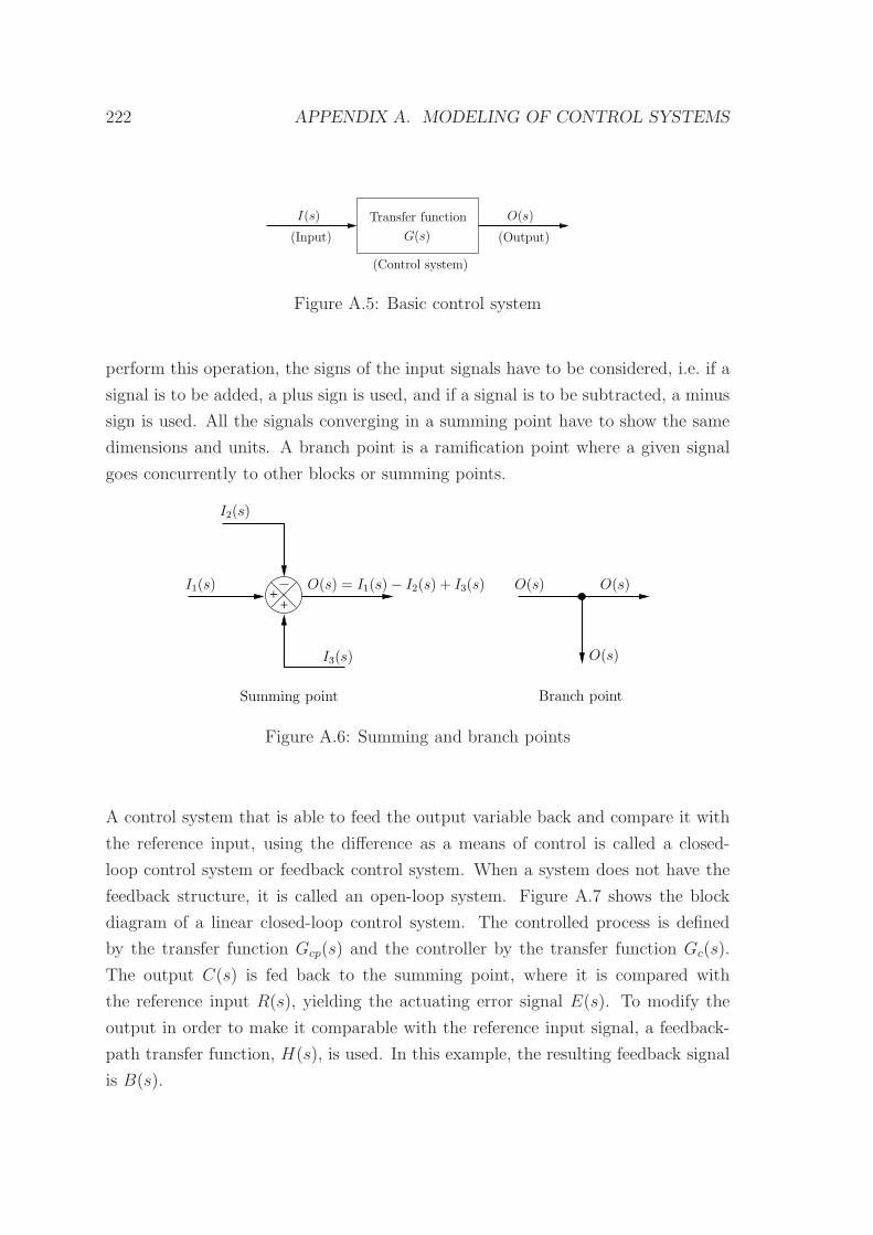
222 APPENDIX A. MODELING OF CONTROL SYSTEMS
G(s)
Transfer function
(Input) (Output)
I(s)
(Control system)
O(s)
Figure A.5: Basic control system
perform this operation, the signs of the input signals have to be considered, i.e. if a
signal is to be added, a plus sign is used, and if a signal is to be subtracted, a minus
sign is used. All the signals converging in a summing point have to show the same
dimensions and units. A branch point is a ramification point where a given signal
goes concurrently to other blocks or summing points.
++
I3(s)
Summing point Branch point
O(s)
O(s) O(s)I1(s)
I2(s)
O(s) = I1(s)− I2(s) + I3(s)
Figure A.6: Summing and branch points
A control system that is able to feed the output variable back and compare it with
the reference input, using the difference as a means of control is called a closed-
loop control system or feedback control system. When a system does not have the
feedback structure, it is called an open-loop system. Figure A.7 shows the block
diagram of a linear closed-loop control system. The controlled process is defined
by the transfer function Gcp(s) and the controller by the transfer function Gc(s).
The output C(s) is fed back to the summing point, where it is compared with
the reference input R(s), yielding the actuating error signal E(s). To modify the
output in order to make it comparable with the reference input signal, a feedback-
path transfer function, H(s), is used. In this example, the resulting feedback signal
is B(s).
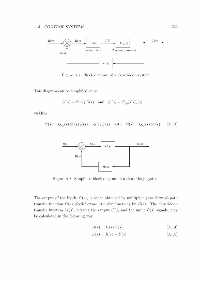
A.3. CONTROL SYSTEMS 223
+
H(s)
B(s)
R(s) E(s)
(Controler) (Controled process)
C(s)Gc(s) Gcp(s)
U(s)
Figure A.7: Block diagram of a closed-loop system
This diagram can be simplified since
U(s) = Gc(s)E(s) and C(s) = Gcp(s)Cc(s)
yielding
C(s) = Gcp(s)Gc(s)E(s) = G(s)E(s) with G(s) = Gcp(s)Gc(s) (A.13)
+
H(s)
G(s)E(s)
B(s)
R(s) C(s)
Figure A.8: Simplified block diagram of a closed-loop system
The output of the block, C(s), is hence obtained by multiplying the forward-path
transfer function G(s) (feed-forward transfer function) by E(s). The closed-loop
transfer function M(s), relating the output C(s) and the input R(s) signals, may
be calculated in the following way
B(s) = H(s)C(s) (A.14)
E(s) = R(s)−B(s) (A.15)
224 APPENDIX A. MODELING OF CONTROL SYSTEMS
substituting Equation (A.13) in Equation (A.15) gives
C(s) = G(s) [R(s)−B(s)] = G(s)R(s)−G(s)B(s) (A.16)
substituting Equation (A.14) in Equation (A.16) yields
C(s) = G(s)R(s)−G(s)H(s)C(s) (A.17)
with some algebraic manipulation, the closed-loop transfer function of the system
may be obtained, reading
M(s) =C(s)
R(s)=
G(s)
1 +G(s)H(s)(A.18)
A.4 Basic control actions
A.4.1 Proportional control
When the output of the controller u(t) is made to be linearly proportional to the
actuating error signal (e(t), the controller is said to have a proportional control
action [118]. The general form of proportional control is
u(t) = Kp e(t) (A.19)
where Kp is a constant, usually named the proportional gain. The controller transfer
function yields
Gc(s) =U(s)
E(s)= Kp (A.20)
A.4.2 Derivative control
In derivative control the controller output signal is proportional to the rate of change
of the actuating error signal e(t) [118]. The general form of derivative control is
u(t) = Kdd e(t)
d t(A.21)
A.4. BASIC CONTROL ACTIONS 225
where Kd is a constant. The transfer function of the derivative controller is
Gc(s) =U(s)
E(s)= Kd s (A.22)
Since d e(t)/d t represents the slope of e(t), the derivative control is mainly an an-
ticipatory type of control. As the controller measures the instantaneous slope of
e(t), it is able to predict the system’s overshoot and produce an adequate correcting
effort, before the overshoot actually occurs.
A.4.3 Integral control
Integral control may be considered the counterpart of derivative control, producing
an output that is proportional to the integral of the error signal [118]. It’s general
form is
u(t) = Ki
∫ t
0
e(t) dt (A.23)
where Ki is a constant. The transfer function of the integral controller yields
Gc(s) =U(s)
E(s)=Ki
s(A.24)
Integral control is very useful for the reduction or elimination of constant steady-
state errors, typically at the cost of a worse transient response.
A.4.4 Proportional-plus-integral-plus-derivative control
The proportional-plus-integral-plus-derivative (PID) controller combines the pro-
portional, integral and derivative control actions. The control signal is a linear
combination of the error, the integral of the error, and the time-rate of the change
of the error. The equation of a controller with this combined action is given by
u(t) = Kp e(t) +Ki
∫ t
0
e(t) dt+Kdd e(t)
d t(A.25)
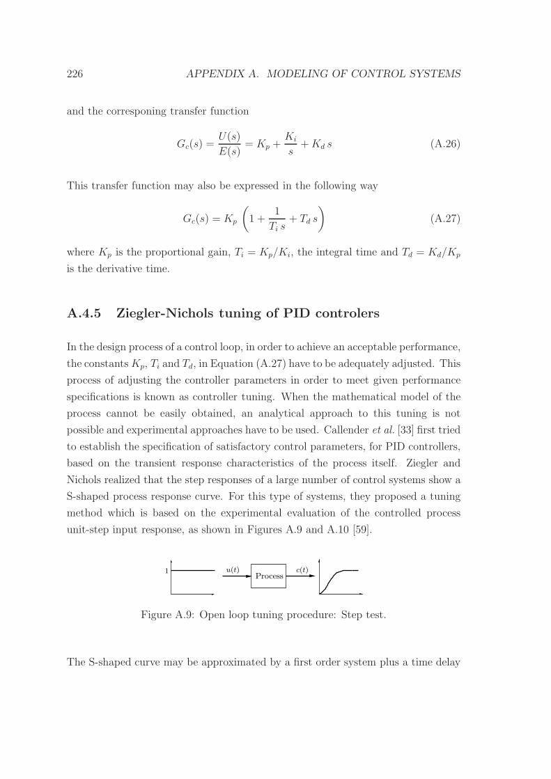
226 APPENDIX A. MODELING OF CONTROL SYSTEMS
and the corresponing transfer function
Gc(s) =U(s)
E(s)= Kp +
Ki
s+Kd s (A.26)
This transfer function may also be expressed in the following way
Gc(s) = Kp
(
1 +1
Ti s+ Td s
)
(A.27)
where Kp is the proportional gain, Ti = Kp/Ki, the integral time and Td = Kd/Kp
is the derivative time.
A.4.5 Ziegler-Nichols tuning of PID controlers
In the design process of a control loop, in order to achieve an acceptable performance,
the constantsKp, Ti and Td, in Equation (A.27) have to be adequately adjusted. This
process of adjusting the controller parameters in order to meet given performance
specifications is known as controller tuning. When the mathematical model of the
process cannot be easily obtained, an analytical approach to this tuning is not
possible and experimental approaches have to be used. Callender et al. [33] first tried
to establish the specification of satisfactory control parameters, for PID controllers,
based on the transient response characteristics of the process itself. Ziegler and
Nichols realized that the step responses of a large number of control systems show a
S-shaped process response curve. For this type of systems, they proposed a tuning
method which is based on the experimental evaluation of the controlled process
unit-step input response, as shown in Figures A.9 and A.10 [59].
1Process
u(t) c(t)
Figure A.9: Open loop tuning procedure: Step test.
The S-shaped curve may be approximated by a first order system plus a time delay
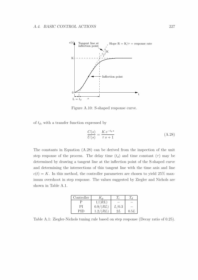
A.4. BASIC CONTROL ACTIONS 227
inflection pointTangent line at
K
τ
t
c(t)
0
K
Inflection point
Slope R = K/τ = response rate
τL = td
Figure A.10: S-shaped response curve.
of td, with a transfer function expressed by
C(s)
U(s)=K e−td s
τ s + 1(A.28)
The constants in Equation (A.28) can be derived from the inspection of the unit
step response of the process. The delay time (td) and time constant (τ) may be
determined by drawing a tangent line at the inflection point of the S-shaped curve
and determining the intersections of this tangent line with the time axis and line
c(t) = K. In this method, the controller parameters are chosen to yield 25% max-
imum overshoot in step response. The values suggested by Ziegler and Nichols are
shown in Table A.1.
Controller Kp Ti Td
P 1/(RL) − −PI 0.9/(RL) L/0.3 −PID 1.2/(RL) 2L 0.5L
Table A.1: Ziegler-Nichols tuning rule based on step response (Decay ratio of 0.25).

228 APPENDIX A. MODELING OF CONTROL SYSTEMS
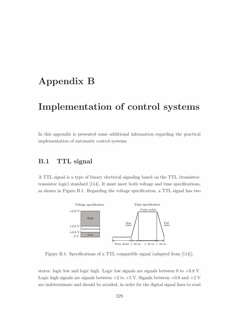
Appendix B
Implementation of control systems
In this appendix is presented some additional information regarding the practical
implementation of automatic control systems.
B.1 TTL signal
A TTL signal is a type of binary electrical signaling based on the TTL (transistor-
transistor logic) standard [114]. It must meet both voltage and time specifications,
as shown in Figure B.1. Regarding the voltage specification, a TTL signal has two
+2.0 V
+5.0 V
+0.8 V
0 V
Risetime
Falltime
Voltage specification
Low
High
Indeterminate
Time specification
< 50 ns > 10 ns < 50 nsTime delay
Pulse width
Figure B.1: Specifications of a TTL compatible signal (adapted from [114]).
states: logic low and logic high. Logic low signals are signals between 0 to +0.8 V.
Logic high signals are signals between +2 to +5 V. Signals between +0.8 and +2 V
are indeterminate and should be avoided, in order for the digital signal lines to read
229
230 APPENDIX B. IMPLEMENTATION OF CONTROL SYSTEMS
the signal correctly [120]. A pulse comprises two parts: the delay, which is the first
part of the pulse (tD), and the pulse width (tW ), which is the remaining part. These
two phases are always in opposite logic levels. In positive logic, the pulse width is
logic high and the delay is logic low. In negative logic, the pulse width is logic low
and the delay is logic high. The time specifications comprise the signal’s maximum
rise and fall times (50 ns) and its minimum pulse with (10 ns) [120]. The rise/fall
time is a measure of how quickly the signal transitions from low to high or from high
to low. For a counter device to be able to detect the rising and falling edges of a
given signal, the transition period must occur within 50 ns or less [114]. In addition
to this time restrain, there must be a minimum time delay between the instant the
counter detects a rising or falling edge until it can detect another rising or falling
edge. This delay is known as the minimum pulse width [114]. The pulse period is
the time it takes for a pulse to complete one cycle (Tp = tD + tW ) while the pulse
frequency is the inverse of the period (fp = 1/Tp). The duty cycle translates the
relation between the pulse width and its corresponding period (duty cycle = tW/Tp).
Regarding the S-ON signal, the logic low level corresponds to the on position of
the servomotor. In this position the servomotor can be operated. Concerning the
signals P-OT and N-OT, the low logic level corresponds to the normal operation
status, meaning that the forward and reverse rotations are allowed. The high level
corresponds to an over-travel situation and hence the forward or/and reverse rotation
is/are prohibited, for the P-OT and N-OT signals respectively. These digital signals
are common to all the external input signal circuits regarding the various control
modes of the servo-system.
B.2 Position-control
When in the position-control mode, the servo-drive controls the servomotor position
by means of a pulse train position reference. When a counter device is used to
generate TTL signals, this is usually called pulse generation. The generated signal
can be a single pulse or a continuous set of pulses, known as a pulse train [114], as
shown in Figure B.2.
In Figure B.3 is shown the block diagram of the position-control VI.
The position-control VI contains a counter and two additional digital output chan-
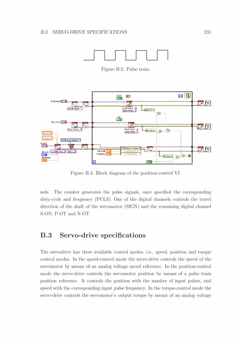
B.3. SERVO-DRIVE SPECIFICATIONS 231
Figure B.2: Pulse train.
Figure B.3: Block diagram of the position-control VI.
nels. The counter generates the pulse signals, once specified the corresponding
duty-cycle and frequency (PULS). One of the digital channels controls the travel
direction of the shaft of the servomotor (SIGN) and the remaining digital channel
S-ON, P-OT and N-OT.
B.3 Servo-drive specifications
The servodrive has three available control modes, i.e., speed, position and torque
control modes. In the speed-control mode the servo-drive controls the speed of the
servomotor by means of an analog voltage speed reference. In the position-control
mode the servo-drive controls the servomotor position by means of a pulse train
position reference. It controls the position with the number of input pulses, and
speed with the corresponding input pulse frequency. In the torque-control mode the
servo-drive controls the servomotor’s output torque by means of an analog voltage
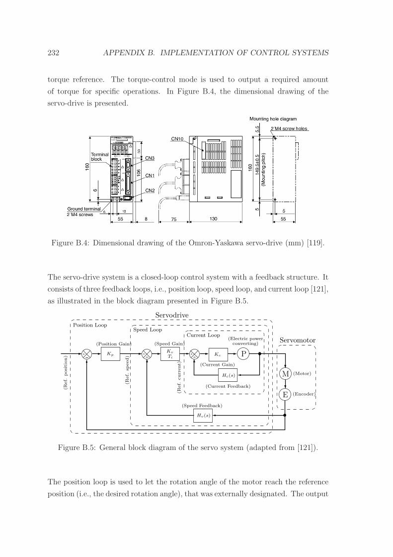
232 APPENDIX B. IMPLEMENTATION OF CONTROL SYSTEMS
torque reference. The torque-control mode is used to output a required amount
of torque for specific operations. In Figure B.4, the dimensional drawing of the
servo-drive is presented.
Figure B.4: Dimensional drawing of the Omron-Yaskawa servo-drive (mm) [119].
The servo-drive system is a closed-loop control system with a feedback structure. It
consists of three feedback loops, i.e., position loop, speed loop, and current loop [121],
as illustrated in the block diagram presented in Figure B.5.
+++
M
E
P
(Electric powerconverting)
Kv
Ti
(Current Gain)
(Speed Feedback)
Hc(s)
Kc
Hv(s)
(Current Feedback)
(Ref.
current)
Servodrive
(Ref.
speed)
(Motor)
(Encoder)
(Position Gain)
Current LoopSpeed Loop
Position Loop
(Ref.
position)
Servomotor
Kp
(Speed Gain)
Figure B.5: General block diagram of the servo system (adapted from [121]).
The position loop is used to let the rotation angle of the motor reach the reference
position (i.e., the desired rotation angle), that was externally designated. The output
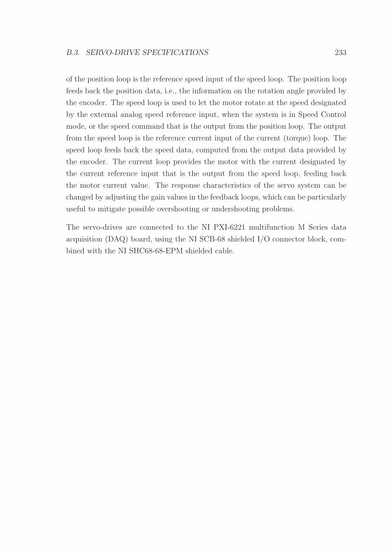
B.3. SERVO-DRIVE SPECIFICATIONS 233
of the position loop is the reference speed input of the speed loop. The position loop
feeds back the position data, i.e., the information on the rotation angle provided by
the encoder. The speed loop is used to let the motor rotate at the speed designated
by the external analog speed reference input, when the system is in Speed Control
mode, or the speed command that is the output from the position loop. The output
from the speed loop is the reference current input of the current (torque) loop. The
speed loop feeds back the speed data, computed from the output data provided by
the encoder. The current loop provides the motor with the current designated by
the current reference input that is the output from the speed loop, feeding back
the motor current value. The response characteristics of the servo system can be
changed by adjusting the gain values in the feedback loops, which can be particularly
useful to mitigate possible overshooting or undershooting problems.
The servo-drives are connected to the NI PXI-6221 multifunction M Series data
acquisition (DAQ) board, using the NI SCB-68 shielded I/O connector block, com-
bined with the NI SHC68-68-EPM shielded cable.

234 APPENDIX B. IMPLEMENTATION OF CONTROL SYSTEMS
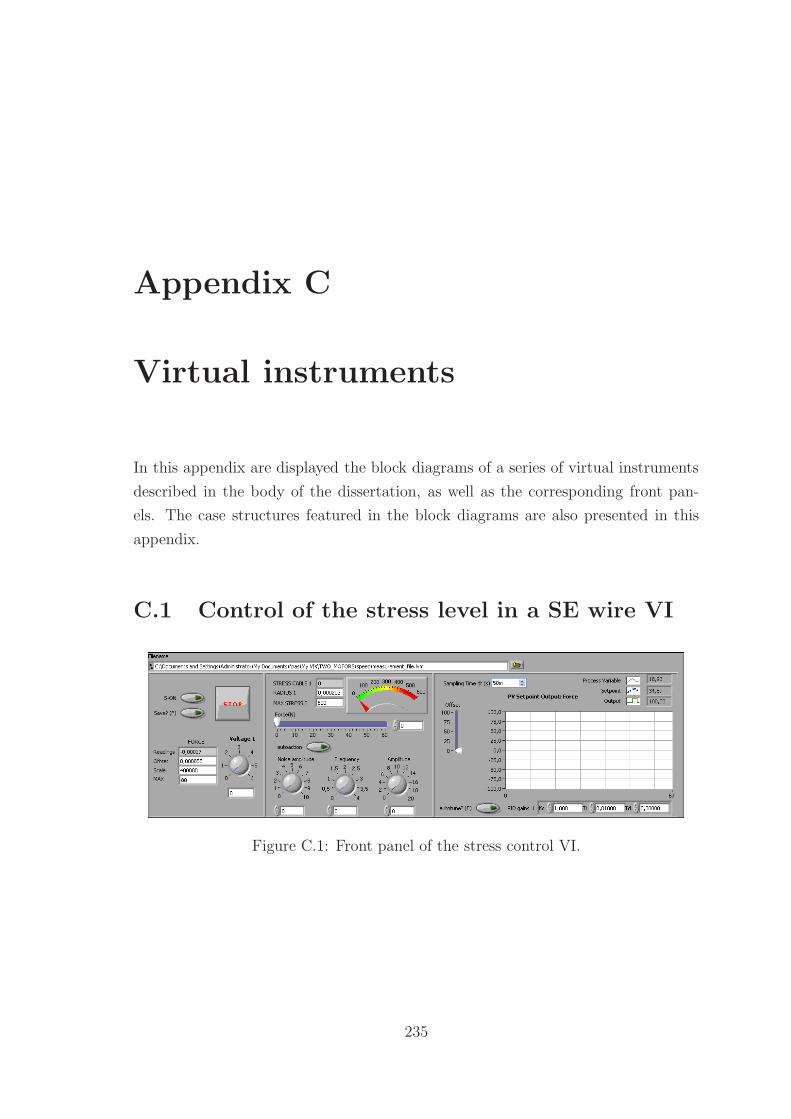
Appendix C
Virtual instruments
In this appendix are displayed the block diagrams of a series of virtual instruments
described in the body of the dissertation, as well as the corresponding front pan-
els. The case structures featured in the block diagrams are also presented in this
appendix.
C.1 Control of the stress level in a SE wire VI
Figure C.1: Front panel of the stress control VI.
235
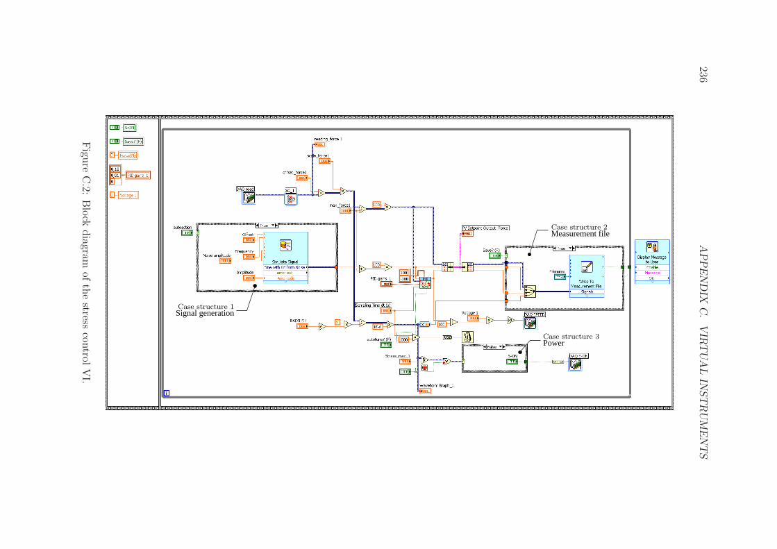
236APPENDIX
C.VIRTUALIN
STRUMENTS
Measurement file
Power
Signal generation
Case structure 2
Case structure 3
Case structure 1
Figu
reC.2:
Block
diagram
ofthestress
control
VI.
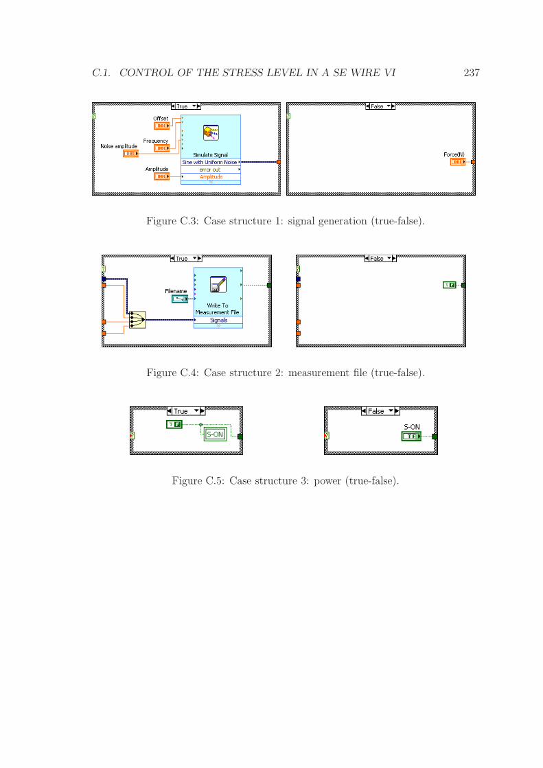
C.1. CONTROL OF THE STRESS LEVEL IN A SE WIRE VI 237
Figure C.3: Case structure 1: signal generation (true-false).
Figure C.4: Case structure 2: measurement file (true-false).
Figure C.5: Case structure 3: power (true-false).
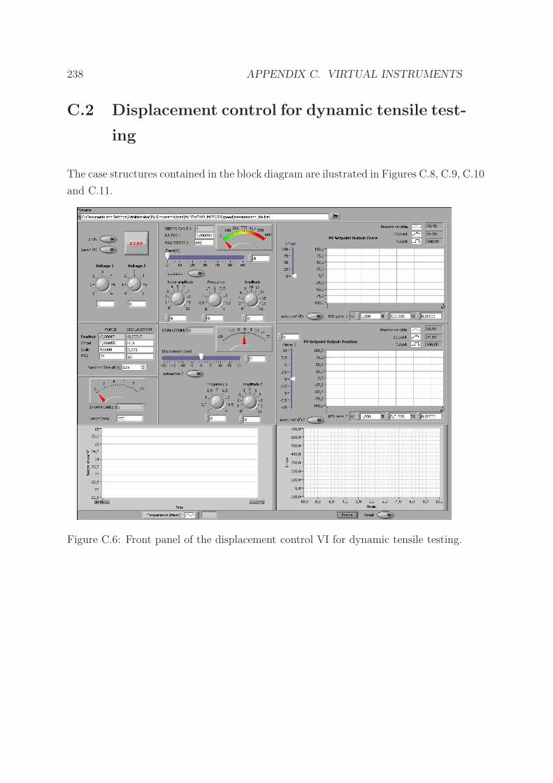
238 APPENDIX C. VIRTUAL INSTRUMENTS
C.2 Displacement control for dynamic tensile test-
ing
The case structures contained in the block diagram are ilustrated in Figures C.8, C.9, C.10
and C.11.
Figure C.6: Front panel of the displacement control VI for dynamic tensile testing.
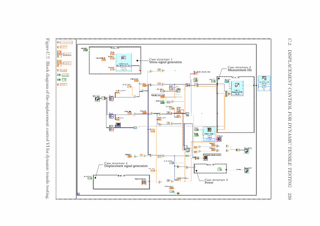
C.2.
DISPLACEMENT
CONTROLFOR
DYNAMIC
TENSILE
TESTIN
G239
Stress signal generation
Displacement signal generation
Measurement file
Power
Case structure 1
Case structure 4
Case structure 2
Case structure 3
Figu
reC.7:
Block
diagram
ofthedisp
lacementcon
trolVIfor
dynam
icten
siletestin
g.
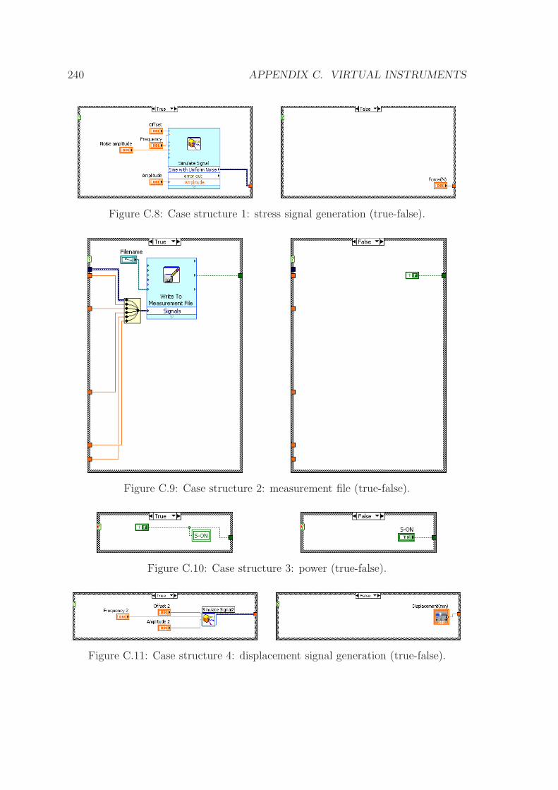
240 APPENDIX C. VIRTUAL INSTRUMENTS
Figure C.8: Case structure 1: stress signal generation (true-false).
Figure C.9: Case structure 2: measurement file (true-false).
Figure C.10: Case structure 3: power (true-false).
Figure C.11: Case structure 4: displacement signal generation (true-false).
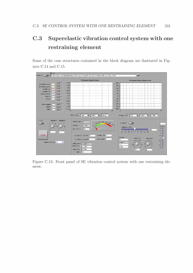
C.3. SE CONTROL SYSTEM WITH ONE RESTRAINING ELEMENT 241
C.3 Superelastic vibration control system with one
restraining element
Some of the case structures contained in the block diagram are ilustrated in Fig-
ures C.14 and C.15.
Figure C.12: Front panel of SE vibration control system with one restraining ele-ment.
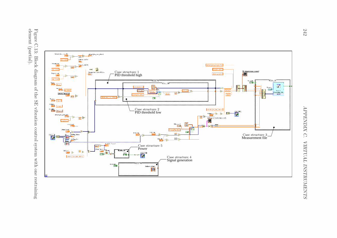
242APPENDIX
C.VIRTUALIN
STRUMENTS
Signal generation
Power
PID threshold high
PID threshold low
Measurement file
Case structure 4
Case structure 5
Case structure 1
Case structure 2
Case structure 3
Figu
reC.13:
Block
diagram
oftheSEvibration
control
system
with
onerestrain
ing
element(partial).
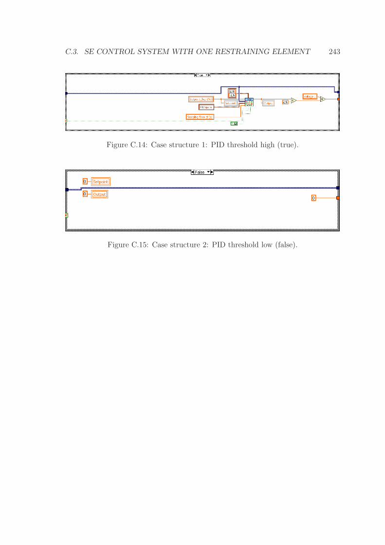
C.3. SE CONTROL SYSTEM WITH ONE RESTRAINING ELEMENT 243
Figure C.14: Case structure 1: PID threshold high (true).
Figure C.15: Case structure 2: PID threshold low (false).
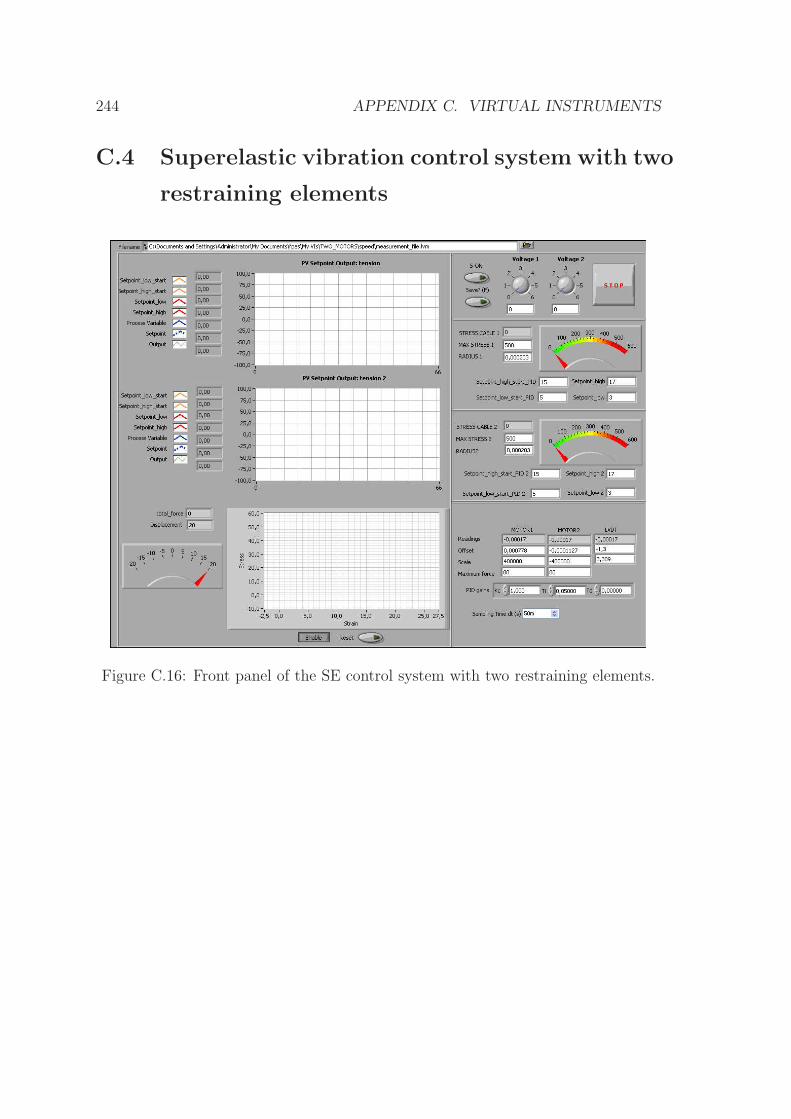
244 APPENDIX C. VIRTUAL INSTRUMENTS
C.4 Superelastic vibration control system with two
restraining elements
Figure C.16: Front panel of the SE control system with two restraining elements.
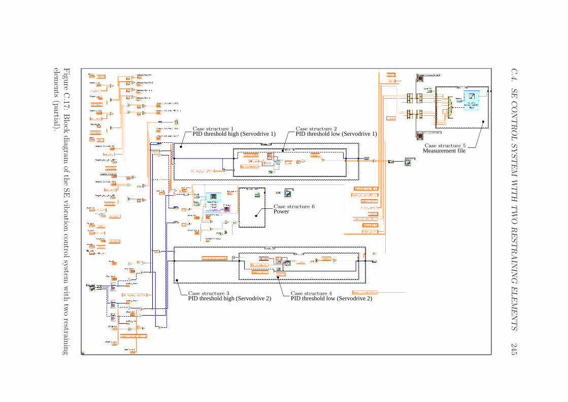
C.4.
SECONTROLSYSTEM
WIT
HTWO
RESTRAIN
ING
ELEMENTS
245
PID threshold high (Servodrive 1) PID threshold low (Servodrive 1)
PID threshold high (Servodrive 2) PID threshold low (Servodrive 2)
Measurement file
Power
Case structure 1 Case structure 2
Case structure 3 Case structure 4
Case structure 5
Case structure 6
Figu
reC.17:
Block
diagram
oftheSEvibration
control
system
with
tworestrain
ing
elements
(partial).
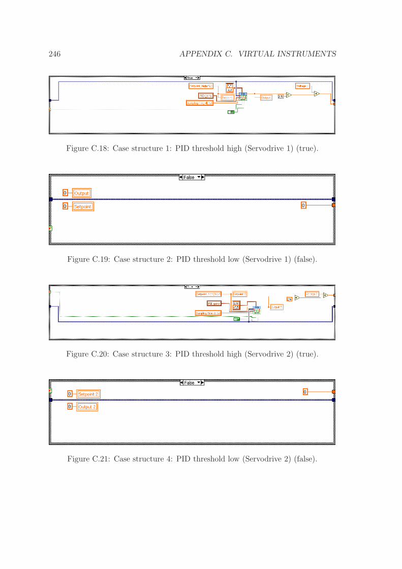
246 APPENDIX C. VIRTUAL INSTRUMENTS
Figure C.18: Case structure 1: PID threshold high (Servodrive 1) (true).
Figure C.19: Case structure 2: PID threshold low (Servodrive 1) (false).
Figure C.20: Case structure 3: PID threshold high (Servodrive 2) (true).
Figure C.21: Case structure 4: PID threshold low (Servodrive 2) (false).
Bibliography
[1] Addington, M., and Schodek, D. Smart Materials and Technologies for
the architecture and design professions. Architectural Press, 2005.
[2] Aiken, I. D., Nims, D. K., Whittaker, A. S., and Kelly, J. M. Testing
of Passive Energy Dissipation Systems. Earthquake Spectra 9, 3 (1993), 335–
369.
[3] Aizawa, S., Kakizawa, T., and Higasino, M. Case studies of smart
materials for civil structures. Smart Materials and Structures 7 (1998), 617–
626.
[4] Alam, M. S., Youssef, M. A., and Nehdi, M. Utilizing shape memory
alloys to enhance the performance and safety of civil infrastructure: a review.
Canadian Journal of Civil Engineering 34 (2007), 1075–1086.
[5] Alam, M. S., Youssef, M. A., and Nehdi, M. Analytical prediction of
the seismic behaviour of superelastic shape memory alloy reinforced concrete
elements. Engineering Structures 30 (2008), 3399–3411.
[6] Amarante dos Santos, F. P., and Cismasiu, C. Comparison Between
Two SMA Constitutive Models for Seismic Applications. Journal of Vibration
and Control 16, 6 (2010), 897–914.
[7] AMETEK Inc. Solartron Metrology Catalogue, 2006.
[8] Andrawes, B., and DesRoches, R. Comparison Between Shape Memory
Alloy Restrainers and and Other Bridge Retrofit Devices. ASCE Journal of
Bridge Engineering 12, 6 (2007), 700–709.
[9] Ascher, U., and Petzold, L. R. Computer methods for ordinary differ-
ential equations and differential-algebraic equations. SIAM, 1998.
247
248 BIBLIOGRAPHY
[10] Ashby, M. F., and Jones, D. R. H. Engineering Materials 2: An In-
troduction to Microstructures, Processing and Design, 3rd ed. Butterworth-
Heinemann, 1986.
[11] Auguet, C., Isalgue, A., Lovey, Martorell, F., and Torra, V.
Metastable effects on martensitic transformation in SMA Part 4. Thermome-
chanical properties of CuAlBe and NiTi observations for dampers in family
houses. Journal of Thermal Analysis and Calorimetry 88, 2 (2007), 537–548.
[12] Auguet, C., Isalgue, A., Lovey, F. C., Ruiz, S., and Torra, V.
Metastable effects on martensitic transformation in SMA Part III. Tentative
temperature effects in a NiTi alloy. Journal of Thermal Analysis and Calorime-
try 89, 2 (2007), 537–542.
[13] Auguet, C., Isalgue, A., Torra, V., Lovey, F. C., and Pelegrina,
J. L. Metastable effects on martensitic transformation in SMA Part VII.
aging problems in NiTi. Journal of Thermal Analysis and Calorimetry 92, 1
(2008), 63–71.
[14] Auricchio, F., Fugazza, D., and Desroches, R. Earthquake Perfor-
mance of Steel Frames with Nitinol Braces. Journal of Earthquake Engineering
10, 4 (2006), 45–66.
[15] Auricchio, F., Fugazza, D., and DesRoches, R. Numerical and Ex-
perimental Evaluation of the Damping Properties of Shape-Memory Alloys.
Journal of Engineering Materials and Technology 128, 3 (2006), 312–319.
[16] Auricchio, F., and Sacco, E. A one-dimensional model for superelas-
tic shape-memory alloys with different elastic properties between austenite
and martensite. International Journal of Non-Linear Mechanics 32, 6 (1997),
1101–1114.
[17] Auricchio, F., and Sacco, E. A temperature-dependent beam for shape-
memory alloys: constitutive modelling, finite-element implementation and nu-
merical simulations. Computer Methods in Applied Mechanics and Engineering
174 (1997), 171–190.
[18] Auricchio, F., Taylor, R. L., and Lubliner, J. Shape-Memory Al-
loys: macromodelling and numerical simulations of the superelastic behaviour.
BIBLIOGRAPHY 249
Computer Methods in Applied Mechanics and Engineering 146 (1997), 281–
312.
[19] Autoliv, Inc. Load limiter. http://www.autoliv.com.
[20] Azadi, B., Rajapakse, R. K. N. D., and Maijer, D. M. One-
dimensional thermomechanical model for dynamic pseudoelastic response of
shape memory alloys. Smart Materials and Structures 15 (2006), 996–1008.
[21] Balandraud, X., Ernst, E., and Soos. Relaxation and creep phenomena
in shape memory alloys. Part II: Stress relaxation and strain creep during
phase transformation. Zeitschrift fur angewandte Mathematik und Physik 51
(2000), 419–448.
[22] Balandraud, X., Ernst, E., and Soos. Monotone strain-stress models
for shape memory alloys hysteresis loop and pseudoelastic behavior. Zeitschrift
fur angewandte Mathematik und Physik 56 (2005), 304–256.
[23] Bekker, A., and Brinson, L. C. Phase Diagram based description of the
hysteresis behavior of shape memory alloys. Acta Metallurgica et Materialia
46, 10 (1997), 3649–3655.
[24] Bhattacharyya, A., Sweeney, L., and G., F. M. Experimental char-
acterization of free convection during thermal phase transformations in shape
memory alloy wires. Smart Materials and Structures 11 (2002), 411–422.
[25] Birman, V. Shape memory elastic foundation and supports for passive vibra-
tion control of composite plates. International Journal of Solids and Structures
45 (2008), 320–335.
[26] Bondaryev, E. N., and Wayman, C. M. Some Stress-Strain-Temperature
Relationships for Shape Memory Alloys. Metallurgical Transactions A 19A
(1988), 2407–2413.
[27] Boroschek, R. L., Farias, G., Moroni, O., and Sarrazin, M. Effect
of SMA braces in a Steel Frame Building. Journal of Earthquake Engineering
11 (2007), 326–342.
[28] Bosch Rexroth AG. Electromechanical Cylinder EMC, 2009. R310EN
3306.
250 BIBLIOGRAPHY
[29] Brinson, L. C. One-Dimensional Constitutive Behavior of Shape Memory
Alloys: Thermomechanical Derivation with Non-Constant Material Functions
and Redefined Martensite Internal Variable. Journal of Intelligent Material
Systems and Structures 4 (1993), 229–242.
[30] Brinson, L. C., and Huang, M. S. Simplifications and Comparisons of
Shape Memory Alloy Constitutive Models. Journal of Intelligent Material
Systems and Structures 7 (1996), 108–114.
[31] Brocca, M., Brinson, L. C., and Bazant, P. Three Dimensional Con-
stitutive Model for Shape Memory Alloys Based on Microplane Model. Journal
of the Mechanics and Physics of Solids 50 (2002), 1051–1077.
[32] Bruno, S., and Valente, C. Comparative response analysis of conven-
tional and innovative seismic protection strategies. Earthquake Engineering
and Structural Dynamics 31 (2007), 1067–1092.
[33] Callender, A., Hartree, D. R., and Porter, A. Time Lag in a Control
System. Phil. Trans. R. Soc. A. London: Cambridge University Press, 1936.
[34] Casciati, S., and Faravelli, L. Structural components in shape memory
alloy for localized energy dissipation. Computers and Structures 86 (2008),
330–339.
[35] Castellano, M. G., Indirli, M., and Martelli, A. Progress of ap-
plication, research and development and design guidelines for shape memory
alloy devices for cultural heritage structures in italy. SPIE Proceedings 4330
(2000), 250–261.
[36] Chang, B. C., Shaw, J. A., and Iadicola, M. A. Thermodynamics of
shape memory alloy wire: modeling, experiments, and application. Continuum
Mechanics and Thermodynamics 18, 1-2 (2006), 83–118.
[37] Chang, L. C., and Read, T. A. Plastic deformation and diffusionless
phase changes in metals - The gold-cadmium beta phase. Trans AIME 189
(1951), 47–52.
[38] Chopra, A. K. Dynamics of Structures: theory and applications to earth-
quake engineering, 2nd ed. Prentice-Hall, Inc., 2001.
BIBLIOGRAPHY 251
[39] Cismasiu, C., and Amarante dos Santos, F. P. Shape Memory Alloys.
Sciyo, 2010.
[40] Cismasiu, C., and Santos, F. P. A. Numerical simulation of superelas-
tic shape memory alloys subjected to dynamic loads. Smart Materials and
Structures 17, 2 (2008), 25–36.
[41] Continental Contitech. Product Range SYNCHROFLEX Timing Belts
- Power Transmission Group. WT6220E 09.06(BL).
[42] Corbi, O. Shape memory alloys and their application in structural oscil-
lations attenuation. Simulation Modelling Practice and Theory 11 (2003),
387–402.
[43] Croci, G. Strengthening the Basilica of St. Francis of Assisi after the Septem-
ber 1997 Earthquake. Structural Engineering International 11, 3 (2001), 207–
210.
[44] De la Flor, S., and Urbina, F. F. Constitutive model of shape memory
alloys: Theoretical formulation and experimental validation. Materials Science
and Engineering, A 427 (2006), 112–122.
[45] DeGarmo, . E., Black, J. T., and Kohser, R. Degarmo’s Materials
and Processes in Manufaturing. Wiley, 2007.
[46] DesRoches, R., and Delemont, M. Seismic retrofit of simply supported
bridges using shape memory alloys. Engineering Structures 24 (2002), 325–
332.
[47] DesRoches, R., McCormick, J., and Delemont, M. Cyclic Properties
of Superelastic Shape Memory Alloy Wires and Bars. Journal of Structural
Engineering 130, 1 (2004), 1–38.
[48] DesRoches, R., Pfeifer, T., Leon, R. T., and Lam, T. Full-Scale Tests
of Seismic Cable Restrainer Retrots for Simply Supported Bridges. Journal of
Bridge Engineering 8, 4 (2003), 191–198.
[49] DesRoches, R., and Smith, B. Shape memory alloys in seismic resistant
design and retrofit: a critical review of their potential applications. ournal of
Earthquake Engineering 7, 3 (2003), 1–15.
252 BIBLIOGRAPHY
[50] Dolce, M., and Cardone, D. Mechanical behaviour of shape memory
alloys for seismic applications 1. Martensite and austenite NiTi bars subjected
to torsion. International Journal of Mechanical Sciences, 43 (2001), 2631–
2656.
[51] Dolce, M., and Cardone, D. Mechanical behaviour of shape memory
alloys for seismic applications 2. Austenite NiTi wires subjected to tension.
International Journal of Mechanical Sciences, 43 (2001), 2657–2677.
[52] Dolce, M., Cardone, D., and Marnetto, R. Implementation and test-
ing of passive control devices based on shape memory alloys. Earthquake
Engineering and Structural Dynamics, 29 (2000), 945–968.
[53] Dolce, M., Cardone, D., Ponzo, F. C., and Valente, C. Shaking
table tests on reinforced concrete frames without and with passive control
systems. Earthquake Engineering and Structural Dynamics 34 (2005), 1687–
1717.
[54] Dolce, M., Donatello, C., and Ponzo, F. C. Shaking-table tests on
reinforced concrete frames with different isolation systems. Earthquake Engi-
neering and Structural Dynamics 36 (2007), 573–596.
[55] Duerig, T. W., and Pelton, A. R. Materials Propreties Handbook: Ti-
tanium Alloys. ASM International, 1994.
[56] Entemeyer, D., Patoor, E., Eberhardt, A., and Berveiller, M.
Strain rate sensitivity in superelasticity. International Journal of Plasticity 16
(2000), 1269–1288.
[57] Faulkner, M. G., Amalraj, J. J., and Bhattacharyya, A. Experi-
mental determination of thermal and electrical properties of Ni-Ti shape mem-
ory wires. Smart Materials and Structures, 9 (2000), 632–639.
[58] Filleul, M. P., and Jordan, L. Torsional properties of Ni-Ti and Copper
Ni-Ti wires: the effect of temperature on physical properties. European Journal
of Orthodontics, 19 (1997), 637–646.
[59] Franklin, G. F., Powell, J. D., and Emami-Naeini, A. Feedback
Control of Dynamic Systems, 3rd ed. Addison-Wesley, 1994.
BIBLIOGRAPHY 253
[60] Fugazza, D. Shape-memory alloy device in earthquake engineering: Me-
chanical propreties, constitutive modelling and numerical simulations. Mas-
ter’s thesis, Rose School. Europeean School of Advanced Studies in Reduction
of Seismic Risk, Pavia, Italy, 2003.
[61] Gadaj, S. P., Nowacki, W. K., and Pieczyska, E. A. Temperature
evolution in deformed shape memory alloy. Journal of Engineering Mechanics
43 (2002), 151–155.
[62] Gandhi, F., and Wolons, D. Characterization of the pseudoelastic damp-
ing behavior of shape memory alloy wires using complex modulus. Smart
Materials and Structures 8 (1999), 49–56.
[63] Govindjee, S., and Garrett, J. H. A computational model for shape
memory alloys. International Journal of Solids and Structures 37 (2000),
735–760.
[64] Graesser, E. J., and Cozzarelli, F. A. Shape-Memory Alloys as New
Materials for Aseismic Isolation. Journal of Engineering Mechanics 117, 11
(1991), 2590–2608.
[65] Graesser, E. J., and Cozzarelli, F. A. A proposed three-dimensional
constitutive model for shape memory alloys. Journal of Intelligent Material
Systems and Structures 5 (1994), 78–89.
[66] Greninger, A. B., and Mooradian, V. G. Strain transformation in
metastable bete copper-zinc and beta copper-tin alloys. Trans AIME 128
(1938), 337–368.
[67] Haland, Y. Evolution of the Three Point Seat Belt - from Yesterday to
Tomorrow. Tech. rep., Autoliv, 2006.
[68] Hamburger, R. O., Foutch, D. A., and Cornell, C. A. Translat-
ing research to practice: FEMA/SAC performance-based design procedures.
Earthquake Spectra 19, 2 (2003), 255–267.
[69] Han, Y. L., Li, Q. S., Li, A. Q., Leung, A. Y. T., and Lin, P. H.
Structural vibration control by shape memory alloy damper. Earthquake En-
gineering & Structural Dynamics 32, 3 (2003), 483–494.
254 BIBLIOGRAPHY
[70] Heinonen, J., Vessonen, I., Klinge, P., and Jarvinen, E. Controlling
stiffness of a frame spring by changing the boundary condition with an SMA
actuator. Computers and Structures 86 (2007), 398–406.
[71] Hodgson, D. E., and Brown, J. W. Using Nitinol Alloys. Shape Memory
Applications, Inc., 2000.
[72] Hoffmann, K. Practical hints for the apllication of strain gages. Hottinger
Baldwin Messtechnik, 1984.
[73] Housner, G. W., Bergman, L. A., Caughey, T. K., Chassiakos,
A. G., Claus, R. O., Masri, S. F., Skelton, R. E., Soong, T. T.,
Spencer, B. F., and Yao, J. T. P. Structural control. past, present, and
future. Journal of Engineering Mechanics 123, 9 (1997), 897–971.
[74] Hsieh, S. F., and Wu, S. K. Lattice parameters of martensite in TiNiZrHf
quaternary shape memory alloys. Journal of Alloys and Compounds 312
(2000), 288–294.
[75] Hwang, J. S., and Ku, S. W. Analytical Modeling of High Damping
Rubber Bearings. Journal of Structural Engineering 123, 8 (1997), 1029–1036.
[76] Incropera, F. P., and DeWitt, D. P. Fundamentals of heat and mass
transfer, 6th ed. John Wiley and Sons, Inc., 2006.
[77] Indirli, M., Castellano, M. G., Clemente, P., and Martelli, A.
Demo-application of shape memory alloy devices: The rehabilitation of the S.
Giorgio Church bell-tower. SPIE Proceedings 4330 (2001), 262–272.
[78] Isalgue, A., Torra, V., Yawny, A., and Lovey, F. Metastable effects
on martensitic transformation in SMA Part VI. the ClausiusClapeyron rela-
tionship. Journal of Thermal Analysis and Calorimetry 91, 3 (2008), 991–998.
[79] Ivshin, Y., and Pence, T. J. A Thermomechanical Model for a One
Variant Shape Memory Material. Journal of Intelligent Material Systems and
Structures 5, 4 (1994), 455–473.
[80] Jansen, L. M., and Dyke, S. J. Semi-Active Control Strategies for MR
Dampers: A Comparative Study. Journal of Engineering Mechanics 126, 8
(2000), 795–803.
BIBLIOGRAPHY 255
[81] Jean, R. D., and Hu, C. T. Shape memory effect by constant-stress ageing
in Ti-50.5 at % Ni alloy. Journal of Materials Science 29 (1994), 449–455.
[82] Johnson, R., Padgett, J. E., Maragakis, M. E., DesRoches, R.,
and Saiidi, M. S. Large scale testing of Nitinol shape-memory alloy devices
for retrofitting of bridges. Smart Materials and Structures 17, 3 (2008).
[83] Jolly, M., Bender, J., and Carlson, J. Properties and applications of
commercial magnetorheological fluids. Journal of Intelligent Material Systems
and Structures 10, 1 (1999), 5–13.
[84] Juntunen, D. Study of Michigan’s Continuous Span Variable Depth T-beam
Bridges. Tech. Rep. R-1374, Michigan Department of Transportation, Testing
and Research Section, 2000.
[85] Kuo, B. C. Automatic Control Systems, 3rd ed. Prentice-Hall, Inc., 1975.
[86] Kurdjumov, G. V., and Khandros, L. G. Doklady Akademii Nauk SSSR
66 (1949), 211–213.
[87] Lacarbonara, W., Bernardini, D., and Vestroni, F. Nonlinear ther-
momechanical oscillations of shape-memory devices. International Journal of
Solids and Structures 41, 5-6 (2004), 1209–1234.
[88] Lagoudas, D. C., Entchev, P. B., and Kumar, P. K. Thermome-
chanical characterization of SMA actuators under cyclic loading. Proceedings
of 2003 ASME International Mechanical Engineering Congress, IMECE2003-
42933 (2003), 211–217.
[89] Lagoudas, D. C., Ravi-Chandar, K., Sarh, K., and Popov, P. Dy-
namic Loading of Polycrystalline Shape Memory Alloy Rods. Mechanics of
materials 35, 7 (2003), 689–716.
[90] Lakes, R. S. Viscoelastic measurement techniques. Review Scientific Instru-
ments 75, 4 (2004), 797–810.
[91] Lammering, R., and Schmidt, I. Experimental investigations on the
damping capacity of NiTi components. Smart Materials and Structures 10
(2001), 853–859.
[92] Laplace, P. S. Theorie analytique des probabilites. Paris, 1812.

256 BIBLIOGRAPHY
[93] Leo, P. H., Shild, T. W., and Bruno, O. P. Transient heat transfer
effects on the pseudoelastic behavior of shape memory wires. Acta Metallurgica
et Materialia 41 (1993), 2477–2485.
[94] Lexcellent, C., and Rejzner, J. Modeling of the strain rate effect, creep
and relaxation of a NiTi shape memory alloy under tension (compression)-
torsional proportional loading in the pseudoelastic range. Smart Materials
and Structures 9 (2000), 613–621.
[95] Li, H., Liu, M., and Ou, J. Vibration mitigation of a stay cable with one
shape memory alloy damper. Structural Control and Health Monitoring 11
(2000), 21–36.
[96] Liang, C., and Rogers, C. A. One-Dimensional Thermomechanical Con-
stitutive Relations for Shape-Memory Materials. Journal of Intelligent Sys-
tems and Structures 1 (1990), 207–234.
[97] Liang, C., and Rogers, C. A. Design of Shape Memory Alloy Springs
With Applications in Vibration Control. Journal of Vibration and Acoustics
115 (1993), 129–135.
[98] Lord Corporation. Lord technical data, MRF-122EG Magneto-Rheological
Fluid, 2008.
[99] Ma, N., Song, G., and Tarefder, R. A. Vibration control of a frame
structure using shape memory alloy braces. Proceedings of the Third Interna-
tional Conference on Earthquake Engineering (2004).
[100] Magee, C. L. Nucleation of martensite. In Phase Transformations, ASM,
Ed. 1970, pp. 115–156.
[101] Matsui, R., Tobushi, H., and Ikawa, T. Transformation-induced creep
and stress relaxation of TiNi shape memory alloy. Proceedings of the Insti-
tution of Mechanical Engineers, Part L: Journal of Materials: Design and
Applications 218, 4 (2004), 343–353.
[102] McCormick, J. Cyclic behavior of shape-memory alloys: material charac-
terization and optimization. PhD thesis, School of Civil and Environmental
Engineering of the Georgia Institute of Technology, 2006.
BIBLIOGRAPHY 257
[103] McCormick, J., DesRoches, R., Fugazza, D., and Auricchio, F.
Seismic Vibration Control Using Superelastic Shape Memory Alloys. Journal
of Engineering Materials and Technology 128, 3 (2006), 294–301.
[104] McCormick, J., Tyber, J., DesRoches, R., Gall, K., and Maier,
H. J. Structural Engineering with NiTi. II: Mechanical Behavior and Scaling.
Journal of Engineering Mechanics 133, 9 (2007), 1019–1029.
[105] Messner, C., and Werner, E. Temperature distribution due to localised
martensitic transformation in SMA tensile test specimens. Computational
Materials Science 26 (2003), 95–101.
[106] Michaud, V. Can shape memory alloy composites be smart? Scripta Mate-
rialia 50 (2004), 249–253.
[107] Miyazaki, S., Imai, T., and Otsuka, K. Effect of Cyclic Deformation
on the Pseudoelasticity Characteristics of Ti-Ni Alloys. Metallurgical and
Materials Transactions A 17, 1 (1986), 115–120.
[108] Modena, C., and Lourenco, P. B. Structural Analysis of Historical
Constructions. Taylor and Francis Group, 2004.
[109] Montecinos, S., Moroni, M., and Sepulveda, A. Superelastic behavior
and damping capacity of CuAlBe alloys. Materials Science and Engineering
A 419 (2005), 91–97.
[110] Motahari, S. A., Ghassemieh, M., and A., A. S. Implementation of
shape memory alloy dampers for passive control of structures subjected to
seismic excitations. Journal of Constructional Steel Research 63 (2007), 1570–
1579.
[111] Moumni, Z., Van Herpen, A., and Riberty, P. Fatigue analysis of shape
memory alloys: energy approach. Smart Materials and Structures 14 (2005),
S287–S292.
[112] Nae, F. A., Tadashige, I., and Matsuzaki, Y. The active tuning of a
shape memory alloy pseudoelastic property. Smart Materials and Structures
13 (2004), 503–511.
[113] National Instruments Corporation. PID Control Toolset User Manual,
2001.
258 BIBLIOGRAPHY
[114] National Instruments Corporation. Data Acquisition and Signal Con-
ditioning Course Manual, 2003.
[115] National Instruments Corporation. Choosing the Right Strain-Gauge
for Your Application, 2006.
[116] National Instruments Corporation. Strain Gauge Configuration Types,
2006.
[117] Ocel, J., DesRoches, R., Leon, R. T., Hess, W. G., Krumme, R.,
Hayes, J., and Sweeney, S. Steel Beam-Column Connections Using Shape
Memory Alloys. Journal of Structural Engineering 130, 5 (2004), 732–740.
[118] Ogata, K. Modern Control Engineering, 3rd ed. Prentice-Hall International,
Inc., 1997.
[119] Omron-Yaskawa Electric Corporation. Sigma-II Series Servodrive
SGDH-* Datasheet. Cat. No. I48E-EN-01.
[120] Omron-Yaskawa Electric Corporation. Sigma-II Series
SGM*H/SGDH user’s Manual. SIEPS80000005C.
[121] Omron-Yaskawa Electric Corporation. Technical Guide: Servo Sys-
tem Startup. Cat. No. I801-E1-1.
[122] Ortın, J., and Delaey, L. Hysteresis in shape-memory alloys. Interna-
tional Journal of Non-Linear Mechanics 37 (2002), 1275–1281.
[123] Ostowari, K., and Souroushian, P. Field Trial of Shape-Memory Based
Rehabilitation System. Tech. Rep. NCHRP-48, IDEA Program, Transporta-
tion Research Board, National Research Council, 2000.
[124] Otsuka, K., and Wayman, C. M., Eds. Shape memory materials (1998),
Cambridge University Press.
[125] Ozbulut, O. E., Mir, C., Moroni, M. O., Sarrazin, M., and
Roschke, P. N. A fuzzy model of superelastic shape memory alloys for
vibration control in civil engineering applications. Smart Materials and Struc-
tures 16 (2007), 818–829.
[126] Pacific Earthquake Engineering Research Center. PEER Strong
Motion Database. http://peer.berkeley.edu/smcat.
BIBLIOGRAPHY 259
[127] Padgett, J. E., DesRoches, R., and Ehlinger, R. Experimental re-
sponse modication of a four-span bridge retrofit with shape memory alloys.
Structural Control and Health Monitoring (2009).
[128] Paiva, A., Savi, M. A., Braga, A. M. B., and Pacheco, P. M. C. L.
A constitutive model for shape memory alloys considering tensile-compressive
asymmetry and plasticity. International Journal of Solids and Structures 42
(2005), 3439–3457.
[129] Panoskaltsis, V. P., and Bahuguna, S. and, S. D. On the thermo-
mechanical modeling of shape memory alloys. International Journal of Non-
Linear Mechanics 39 (2004), 709–722.
[130] Pappas, P., Bollas, D., Parthenios, J., Dracopoulos, V., and Gali-
otis, C. Transformation fatigue and stress relaxation of shape memory alloy
wires. Smart Materials and Structures 16 (2007), 2560–2570.
[131] Patoor, E., Lagoudas, D. C., Entchev, P., Brinson, C., and Gao,
X. Shape memory alloys, Part I: General properties and modeling of single
crystals. Mechanics of Materials 38 (2006), 391–429.
[132] Pieczyska, E. A., Gadaj, S. P., Nowacki, W. K., Makino, Y., and
Tobushi, H. Characteristics of energy storage and dissipation in TiNi shape
memory alloy. Science and Technology of Advanced Materials 6 (2005), 889–
894.
[133] Pieczyska, E. A., Gadaj, S. P., Nowacki, W. K., and Tobushi, H.
Phase-Transformation Fronts Evolution for Stress and Strain Controlled Ten-
sion Tests in TiNi Shape Memory Alloy. Experimental Mechanics 46 (2006),
531–542.
[134] Pieczyska, E. A., Gadaj, S. P., Nowacki, W. K., and Tobushi, H.
Stress relaxation during superelastic behavior of TiNi shape memory alloy.
International Journal of Applied Electromagnetics and Mechanics 23 (2006),
3–8.
[135] Piedboeuf, M. C., and Gauvin, R. Damping behaviour of shape memory
alloys: strain amplitude, frequency and temperature effects. Journal of Sound
and Vibration 214, 5 (1998), 885–901.
260 BIBLIOGRAPHY
[136] Potapov, P. L., Shelyakov, A. V., and Schryvers, D. On the crystal
structure of tini-cu martensite. Scripta Materialia 44 (2001), 1–7.
[137] Potapov, P. L., Shelyakov, A. V., and Schryvers, D. A one-
dimensional strain-rate-dependent constitutive model for superelastic shape
memory alloys. Smart Materials and Structures 16 (2007), 191–197.
[138] Pungor, E. A Practical Guide to Instrumental Analysis. CRC Press LLC,
1995.
[139] Qiang, P., and Cho, C. The Investigation of a Shape Memory Alloy Micro-
Damper for MEMS Applications. Sensors 7 (2007), 1887–1900.
[140] Quanser Inc. Quanser Shake Table II User Manual, 2007. Document Num-
ber 632/Revision 3.10.
[141] Reynolds, D. R. A Nonlinear Thermodynamic Model for Phase Transitions
in Shape Memory Alloy Wires. PhD thesis, Rice University, Houston, Texas,
2003.
[142] Saadat, S., Noori, M., Davoodi, H., Suzuki, Y., and Masuda, A.
Using NiTi SMA tendons for vibration control of coastal structures. Smart
Materials and Structures 10 (2001), 695–704.
[143] Saadat, S., Salichs, J., Noori, M., Hou, Z., Davoodi, H., Bar-on,
I. Suzuki, Y., and Masuda, A. An overview of vibration and seismic
applications of NiTi shape memory alloy. Smart Materials and Structures 11
(2002), 218–229.
[144] Saint-Sulpice, L., Chirani, S. A., and Calloch, S. Super-elastic be-
havior of shape memory alloys under proportional cyclic loadings. Materials
Science and Engineering A 481-482 (2008), 174–177.
[145] Saint-Sulpice, L., Chirani, S. A., and Calloch, S. A 3D super-elastic
model for shape memory alloys taking into account progressive strain under
cyclic loadings. Mechanics of Materials 41 (2009), 12–26.
[146] Seelecke, S. Torsional vibration of a shape memory wire. Continuum Me-
chanics and Thermodynamics 9 (1997), 165–173.
BIBLIOGRAPHY 261
[147] Seelecke, S. Modeling the dynamic behavior of shape memory alloys. In-
ternational Journal of Non-Linear Mechanics 37 (2002), 1363–1374.
[148] Seelecke, S., Heintze, O., and Masuda, A. Simulation of earthquake-
induced structural vibrations in systems with SMA damping elements. SPIE
Smart Structures and Materials 4697 (2002).
[149] Shook, D. A., Roschke, P. N., and Ozbulut, O. E. Superelastic semi-
active damping of a base-isolated structure. Structural Control and Health
Monitoring 15 (2008), 746–768.
[150] Song, G., Ma, N., and Li, H. N. Applications of shape memory alloys in
civil structures. Engineering Structures 28 (2006), 1266–1274.
[151] Soong, T. T., and Spencer, B. F. Supplemental energy dissipation:
state-of-the-art and state-of-the-practice. Engineering Structures 24 (2002),
243–259.
[152] Soroushian, P., Ostowari, K., and Nossoni, A.and Chowdhury,
B. Repair and strengthening of concrete structures through applications of
corrective posttensioning forces with shape memory alloys. Transportation
Research Record 1770 (2001), 2026.
[153] Spencer, B. F., and Nagarajaiah, S. State of the Art of Structural
Control. Journal of Structural Engineering 129, 7 (2009), 845–856.
[154] Spencer, B. F., and Sain, M. K. Controlling Buildings: A New Frontier in
Feedback. Special Issue of the IEEE Control Systems Magazine on Emerging
Technology 17, 6 (1997), 1935.
[155] Sun, S., and Rajapakse, R. K. N. D. Simulation of pseudoelastic be-
haviour of sma under cyclic loading. Computational Materials Science 28
(2003), 663–674.
[156] Symans, M. D., and Constantinou, M. C. Semi-active control systems
for seismic protection of structures: a state-of-the-art review. Engineering
Structures 21 (1999), 469–487.
[157] Tamai, H., and Kitagawa, Y.and Fukuta, T. Application of sma rods to
exposed-type column bases in smart structural systems. In Proc., 13th World
Conf. on Earthquake Engineering, no. 1884.
262 BIBLIOGRAPHY
[158] Tamai, H., and Kitagawa, Y. Pseudoelastic behavior of shape memory
alloy wire and its application to seismic resistance member for building. Com-
putational Materials Science 25, 1-2 (2002), 218–227.
[159] Tanaka, K., Kobayashi, S., and Sato, Y. Thermomechanics of trans-
formation pseudoelasticity and shape memory effect in alloys. International
Journal of Plasticity 2 (1986), 59–72.
[160] Tanaka, K., Nishimura, F., Hayashi, T., Tobushi, H., and Lexcel-
lent, C. Phenomenological analysis on subloops and cyclic behavior in shape
memory alloys under mechanical and/or thermal loads. Mechanics of Materi-
als 19 (1995), 281–292.
[161] Thomas, L. C. Heat Transfer. Prentice-Hall, Inc., 1992.
[162] Tobushi, H., Iwanaga, H., Tanaka, K., Hori, T., and Sawada, T.
Deformation behaviour of TiNi shape memory alloy subjected to variable stress
and temperature. Continuum Mechanics and Thermodynamics 3 (1991), 79–
93.
[163] Tobushi, H., Iwanaga, H., Tanaka, K., Hori, T., and Sawada, T.
Stress-strain-temperature relations of TiNi shape memory alloy suitable for
thermomechanical cycling. JSME International Journal. Series A, Solid Me-
chanics and Material Engineering 35, 3 (1992), 271–277.
[164] Tobushi, H., Shimeno, Y., Hachisuka, T., and Tanaka, K. Influence
of strain rate on superelastic properties of TiNi shape memory alloy. Mechanics
of Materials 30 (1998), 141–150.
[165] Torra, V., Isalgue, A., Martorell, F., Terriault, P., and Lovey,
F. Built in dampers for family homes via SMA: An ANSYS computation
scheme based on mesoscopic and microscopic experimental analyses. Engi-
neering Structures 29 (2007), 1889–1902.
[166] Torra, V., Pelegrina, J., Isalgue, A., and Lovey, F. Metastable
effects on martensitic transformation in SMA (I): Recoverable effects by the
action of thermodynamic forces in parent phase. Journal of Thermal Analysis
and Calorimetry 81 (2005), 131–135.
BIBLIOGRAPHY 263
[167] van der Wijst, M. W. M. Shape Memory Alloys featuring Nitinol. Tech.
Rep. 256199, Technische Universiteit Eindhoven, 1992.
[168] Van Humbeeck, J., and Liu, Y. Shape memory alloys as damping mate-
rials. Materials Science Forum (2000), 327–338.
[169] Vitiello, A., Giorleo, G., and Morace, R. E. Analysis of thermome-
chanical behaviour of Nitinol wires with high strain rates. Smart Materials
and Structures 14 (2005), 215–221.
[170] Vitiello, A., Squillace, A., and U., P. Characterization of Nitinol under
torsional loads through a numerical implementation of the Boyd-Lagoudas con-
stitutive model and comparison of the results with experimental data. Smart
Materials and Structures 16 (2007), 76–82.
[171] Sittner, P., and Novak, V. L. Load Partitioning in Shape Memory Alloy
Polycrystals Studied by In-situ Neutron Diffraction and Modeling. Presented
at IUTAM2001 Symposium on Mechanics of Martensitic Phase Transforma-
tion in Solids (2001), 179–188.
[172] Wang, X., Xu, B., and Yue, Z. Phase transformation behavior of pseu-
doelastic NiTi shape memory alloys under large strain. Journal of Alloys and
Compounds 463 (2008), 417–422.
[173] Weisstein, E. W. Polygon Area. From MathWorld–A Wolfram Web Re-
source.http://mathworld.wolfram.com/PolygonArea.html.
[174] Wilde, K., Gardoni, P., and Fujino, Y. Base isolation system with
shape memory alloy device for elevated highway bridges. Engineering Struc-
tures 22 (2000), 222–229.
[175] Yoshida, I., Ono, T., and Asai, M. Internal friction of Ti-Ni alloys.
Journal of Alloys and Compounds 310 (2000), 339–343.
[176] Zhang, Y., and Zu, S. Seismic Response Control of Building Structures
with Superelastic Shape Memory Alloy Wire Dampers. Journal of Engineering
Mechanics 134, 3 (2007), 240–251.
[177] Zhang, Y., and Zu, S. A shape memory alloy-based reusable hysteretic
damper for seismic hazard mitigation. Smart Materials and Structures 16
(2007), 1603–1623.

264 BIBLIOGRAPHY
[178] Zuo, X. B., Chang, W., Li, A. Q., and Chen, Q. F. Design and
experimental investigation of a superelastic SMA damper. Materials Science
and Engineering A 438-440 (2006), 1150–1153.

Index
Active control, 141
Applications in existing civil engineering
structures, 31
Austenite, 40
Base isolation system, 24
Biot number, 86
Bridge hinge restrainers, 25
Clamps, 175
Clausius-Clapeyron coefficient, 14, 46
Constitutive model, 75
Convection, 85
Cumulative creep, 62
Cyclic properties, 61
Delay, 230
Differential Scanning Calorimetry, 44
Displacement-sensor, 172
Electromechanical cylinder, 174
Equivalent viscous damping, 18
Euler method, 90
Exponential kinetic law, 81
Force-sensor, 164
Gauge-factor, 167
Internal friction, 16
Internal loops, 50
Kinetic law, 79
Linear actuators, 173
Linear kinetic law, 80
Martensite, 40
Martensite fraction, 76
Martensitic transformation, 8
Mechanical law, 76
Mounting system, 175
Newmark method, 114
Nitinol, 40
Passive control, 141
PID, 180
PID tunning, 184
Position-control, 230
Pre-strain, 113
Prototype, 176
Pulse, 230
Pulse width, 230
Rate-dependent model, 92
Rate-independent model, 88
Reuss model, 76
Reuss scheme, 79
SE restraining area, 133
Semi-active control, 141
Servo-drive, 174
Servomotor, 174
Shake-table, 176
Shape-Memory Alloy, 7
265

266 INDEX
Shape-Memory effect, 14
Simple serial model, 76
Speed-control mode, 179
Steady-state response, 113
Strain-creep, 66
Stress-relaxation, 66
Structural connections, 29
Superelasticity, 11
Tensile properties, 42
Thermal effects, 83
Transformation fronts, 59
Transformation temperatures, 44
Transient response, 113
TTL signal, 229
Voight model, 76
Voight scheme, 78
Wheatstone bridge, 165
Ziegler-Nichols rule, 184