vertical structure variability and equatorial waves during central...
TRANSCRIPT

Vertical structure variability and equatorial waves during centralPacific and eastern Pacific El Ninos in a coupled generalcirculation model
B. Dewitte • J. Choi • S.-I. An • S. Thual
Received: 24 January 2011 / Accepted: 3 October 2011 / Published online: 20 October 2011
� Springer-Verlag 2011
Abstract Recent studies report that two types of El Nino
events have been observed. One is the cold tongue El Nino
or Eastern Pacific El Nino (EP El Nino), which is charac-
terized by relatively large sea surface temperature (SST)
anomalies in the eastern Pacific, and the other is the warm
pool El Nino (a.k.a. ‘Central Pacific El Nino’ (CP El Nino)
or ‘El Nino Modoki’), in which SST anomalies are con-
fined to the central Pacific. Here the vertical structure
variability of the periods during EP and CP is investigated
based on the GFDL_CM2.1 model in order to explain the
difference in equatorial wave dynamics and associated
negative feedback mechanisms. It is shown that the mean
stratification in the vicinity of the thermocline of the cen-
tral Pacific is reduced during CP El Nino, which favours
the contribution of the gravest baroclinic mode relatively to
the higher-order slower baroclinic mode. Energetic Kelvin
and first-meridional Rossby wave are evidenced during the
CP El Nino with distinctive amplitude and propagating
characteristics according to their vertical structure (mostly
first and second baroclinic modes). In particular, the first
baroclinic mode during CP El Nino is associated to the
ocean basin mode and participates to the recharge process
during the whole El Nino cycle, whereas the second
baroclinic mode is mostly driving the discharge process
through the delayed oscillator mechanism. This may
explain that the phase transition from warm to neutral/cold
conditions during the CP El Nino is delayed and/or
disrupted compared to the EP El Nino. Our results have
implications for the interpretation of the variability during
periods of high CP El Nino occurrence like the last decade.
1 Introduction
Many recent studies have showed that there exists more
than one type of El Nino (or El Nino Southern Oscillation;
ENSO) based on spatial distributions of SST (Larkin and
Harrison 2005a, b; Ashok et al. 2007; Weng et al. 2007;
Kao and Yu 2009; Kug et al. 2009; Yeh et al. 2009) or
physically separated modes (Neelin et al. 1998; Jin et al.
2003; Bejarano and Jin 2008). So far, the ENSO has been
categorized into two types of El Nino, the traditional Cold
Tongue El Nino or Eastern Pacific El Nino (hereafter EP El
Nino) that consists in SST anomaly developing and peak-
ing in the eastern equatorial Pacific and the so-called
Modoki El Nino (Ashok et al. 2007) or Central Pacific El
Nino (Kao and Yu 2009; hereafter CP El Nino) that con-
sists in SST anomaly developing and persisting in the
central Pacific. Whereas the dynamics of the EP El Nino
has been well documented (McPhaden et al. 1998), the
observed increased occurrence of the CP El Nino during
the last decades (Yeh et al. 2009) has led the community to
investigate the mechanisms responsible for the triggering,
development and decay of this different flavour of El Nino.
Recent studies (Yu et al. 2010; Yu and Kim 2011) sug-
gested an extratropical SLP forcing mechanism to explain
the triggering of the CP El Nino whereas Yu and Kim
(2010a) argued the decay of the CP El Nino is affected
by the warm or cold phase of the EP El Nino. Kug et al.
(2009) documented from the NCEP Reanalysis some
aspects of the evolution of this kind of event, highlighting
differences in the transition mechanism, namely the
B. Dewitte (&) � S. Thual
LEGOS/IRD, 14 av. Edouard Belin,
31400 Toulouse, France
e-mail: [email protected]
J. Choi � S.-I. An
Yonsei University, Seoul, South Korea
123
Clim Dyn (2012) 38:2275–2289
DOI 10.1007/s00382-011-1215-x
recharge and discharge process of the equatorial heat
content. In particular, they showed that the zonal advective
feedback (i.e. zonal advection of mean SST by anomalous
zonal currents) plays a crucial role in the development of
SST anomalies associated with the CP El Nino, while the
thermocline feedback is the key process during the EP El
Nino. Kug et al. (2010) confirms these findings using a
long-term model simulation that shows the major observed
features of both types of El Nino, namely the GFDL model
(Wittenberg et al. 2006). They further suggest that the
frequency of occurrence of the CP El Nino event is related
to the mean state of the tropical Pacific according to a two-
way interaction process that makes the CP El Nino events
rectifying on the mean warm pool, which in turn may
favour the enhancement of anomalous zonal advection of
mean temperature and so the development of the CP El
Nino. Such mechanism was documented in more details in
Choi et al. (2011) and is consistent with recent observed
trend in both the warm pool (Cravatte et al. 2009) and the
El Nino variability (Lee and McPhaden 2010). It is based
on the observation that the discharge process during CP El
Nino is weak and operates mainly through thermal damp-
ing (heat flux) rather than through equatorial wave
dynamics like for the EP El Nino.
The reason for such difference in dynamics between CP
and EP El Nino remains unclear. From a theoretical per-
spective, it is actually expected that, in a situation where
the zonal advective feedback is dominant, the ENSO mode
is destabilized by the gravest ocean basin mode, resulting
in fast westward propagating SST anomalies (An and Jin
2001). If the zonal advection is a dominant process during
the development of CP El Nino (Kug et al. 2009, 2010), the
ocean basin mode may therefore be favoured (Jin and
Neelin 1993; Kang et al. 2004), which may be propitious
for the equilibrium between thermal damping and advec-
tion at basin scale. The difference of the recharge-dis-
charge process between both types may actually results
from a different dynamical adjustment that thereby modi-
fies the heat flux equilibrium at the air-sea interface. This
calls for investing the wave dynamics during the CP El
Nino and the relevance of the negative feedbacks of ENSO
(Neelin et al. 1998), namely the so-called delayed oscillator
feedback (Schopf and Suarez 1988; Suarez and Schopf
1989) and the zonal advective feedback proposed by Picaut
et al. (1996). Both are based on the delayed effect of
reflected equatorial wave at the meridional boundaries on
the vertical and zonal advection and are influential on the
characteristics of the ENSO coupled instabilities (Jin and
Neelin 1993; Neelin and Jin 1993; Dewitte 2000). As a
preliminary step towards the evaluation of these feedbacks,
it appears necessary to document the vertical structure and
propagating characteristics of the equatorial waves during
CP El Nino, which is central for ENSO dynamics.
This is the objective of this paper which can be seen as
an extension of Kug et al. (2010) since it takes advantage
of the long-term simulation of the GFDL model (Witten-
berg et al. 2006) that simulates the major observed features
of both types of El Nino, incorporating the distinctive
patterns of each oceanic and atmospheric variable. Due to
the time span of the simulation (500 years), statistical
significance is achieved. Actually this model simulates CP
and EP El Nino events that strikingly resemble two recent
events representative of both type of El Nino events,
namely the 1997/98 El Nino (EP El Nino) and the 2004/05
El Nino (CP El Nino). As an illustration, the Fig. 1 rep-
resents the time evolution of SST anomalies during these
events both for the GFDL model composite and for the
SODA reanalysis (Carton and Giese 2008). Model and
Reanalysis data share many common features, which
includes, the relative amplitude of the anomalies between
El Nino types, the longitudinal location of peak SST
anomalies and the seasonal evolution (see Kug et al. (2010)
for further description of the ENSO composites of the
GFDL model). Due to the compositing procedure (and
model biases), the anomalies in the GFDL model are
weaker than for the two observed events. Despite this
limitation, the simulation offers the opportunity to inves-
tigate the vertical structure variability and associated
equatorial wave during both type of El Nino, which can
provide material for the interpretation of observed recent
events. Yu and Kim (2010b) also report that the GFDL
model is among the group of six models of the CMIP3
(World Climate Research Programme’s Coupled Model
Intercomparison Project phase 3) that best simulate both
the EP and CP El Ninos in terms of their intensity ratio.
The paper is organized as follows: The Sect. 2 describes
the data sets and the method. The Sect. 3 is devoted to the
analysis of the vertical structure variability whereas Sect. 4
documents the equatorial wave characteristics during both
types of events. The Sect. 5 is a discussion followed by
concluding remarks.
2 Data sets and method
2.1 The GFDL_CM2.1 model
The pre-industrial GFDL CM2.1 long-term simulation
spanning 500 years is used. The ocean component is ocean
model version 3.1 (Gnanadesikan et al. 2006; Griffies et al.
2005), which is based on Modular Ocean Model version 4
(MOM4) code. The resolution is 50 vertical levels and a
1� 9 1� horizontal grid telescoping to 1/3 meridional
spacing near the equator. The vertical grid spacing is a
constant 10 m over the top 220 m. The atmospheric com-
ponent is the GFDL AM2p13 atmospheric model. The
2276 B. Dewitte et al.: Vertical structure variability and equatorial waves during Central Pacific
123

resolution is 24 vertical levels, and 2� latitude by 2.5�longitude grid spacing. The dynamic core is based on a
finite volume (Lin 2004). Air-sea fluxes are computed
based on 1-h intervals. For a detailed model description,
refer to Delworth et al. (2006) and Wittenberg et al. (2006).
The data are available in the CMIP3 archives (https://www.
esg.llnl.gov:8443/home/publicHomePage.do).
Following Kug et al. (2010), in order to define two-types
of El Nino events, we use modified NINO3 and NINO4
SST indices because the climatological cold tongue
extends farther west than observational data would suggest,
and because ENSO variability is also shifted slightly to the
west in the model. Wittenberg et al. (2006) noted that the
simulated patterns of tropical Pacific SST, wind stress, and
precipitation variability are displaced longitudinally by
20–30� west of the observed pattern. New indices are
therefore defined NINO3m SST as the averaged SST over
170�–110�W, 5�S–5�N, and NINO4m SST as the averaged
SST over 140�E–170�W, 5�S–5�N. Note that the area thus
defined is shifted about 20� longitude to the west compared
to the conventionally defined area. Based on the two indi-
ces, all El Nino events are initially selected when either of
the two indices is greater than 0.5�C during NDJ. A total of
205 El Nino events were selected. We classified them as CP
or as EP. El Nino events with a NINO4m SSTA greater than
the NINO3m SSTA were considered CP, and those with a
NINO3m SSTA greater than the NINO4m SSTA were
labelled EP. We acknowledge that this division into only
two groups is a limitation. Some events exhibiting similar
magnitudes for NINO3m and NINO4m indices, though in
Fig. 1 Time longitude section
of SST anomalies along the
equator during the (top)
1997/1998 El Nino and the
(bottom) 2004/2005 El Nino
from (right) SODA and the
(left) GFDL model. The whitethick line indicates the position
of the 28�C isotherm at the
surface. Units are �C
B. Dewitte et al.: Vertical structure variability and equatorial waves during Central Pacific 2277
123
reality mixed, were still placed in one of the two groups.
Based on our definitions, a total of 121 events were clas-
sified as CP El Nino events and 84 as EP El Nino events.
The reader is invited to refer to Kug et al. (2010) for
details on how this procedure allows differentiating the two
events in terms of dynamics and phenology.
2.2 Estimation of equatorial waves
A modal decomposition of the GFDL simulation was
performed following a similar method than in Dewitte et al.
(1999). As a first step, a vertical mode decomposition of
the model mean stratification is sought at each longitude
along the equator leading to the structure functions Fn(x,z).
Zonal currents {u(x,y,z,t)} and pressure {p(x,y,z,t)} anom-
alies are then estimated relative to the climatological sea-
sonal cycle and these fields are projected on the vertical
structure functions Fn(x,z), leading to the baroclinic mode
contributions to sea level and current anomalies. This
implies computing the following quantity:
qðx; y; z; tÞ j Fnðx; zÞh i ¼Z0
HðxÞ
qðx; y; z; tÞFnðx; zÞdz;
H(x) being the ocean depth, and q being u or p. As a final
step, the baroclinic modes are projected onto the theoretical
meridional modes (Kelvin and Rossby modes) associated to
the Fn(x,z) to derive the Kelvin and Rossby waves coeffi-
cients. The reader is invited to refer to Dewitte et al. (1999)
for more technical details. To derive the vertical modes,
usually, the mean stratification over the entire model sim-
ulation is used. Here, to take into account that there is a
change in mean density (e.g. mean stratification) at low
frequency, we used the mean temperature and salinity
profiles corresponding to the periods of high and low CP El
Nino occurrence. Kug et al. (2010) defined a frequency
index (number of occurrences) of both types of El Nino,
defined by the number of events in a sliding 20-years period.
They show that there is a strong negative correlation
between the two indices, and that the periods of large CP
(EP) occurrence corresponds to a warmer (cooler) SST in
the central Pacific (their figure 13). Choi et al. (2011) fur-
ther showed that the vertical temperature in the upper
300 m is also significantly different between the two peri-
ods (see also Fig. 2), which can be influential on the vertical
mode functions. The vertical mode decomposition was
therefore performed for the mean density corresponding to
period of high (low) CP El Nino occurrence for the CP (EP)
composite. The amplitudes of the Kelvin wave and the first-
meridional mode of Rossby wave are then derived by
projecting the pressure and zonal current baroclinic con-
tributions onto the theoretical meridional modes.
The Kelvin (Rossby) wave contribution to thermocline
anomalies was also estimated following Dewitte (2000),
namely considering the vertical isotherm displacements at
the depth of the mean thermocline and the hydrostatic
approximation. For the Kelvin wave, it writes as follows:
fAKn ¼g
N2ðx; z ¼ hÞdFn
dzðx; z ¼ hÞAKnðx; y; tÞ
where AKn is the Kelvin wave contribution to sea level
anomalies for the nth baroclinic mode. h is the mean
thermocline depth approximated as the depth of the 17�C
isotherm of the mean temperature like in Choi et al. (2011).
N2 and Fn are the Brunt-Vaisala frequency and the nth
vertical mode function respectively associated to the mean
stratification during the periods of high and low CP El Nino
occurrence. The estimation of the equatorial wave contri-
bution to thermocline anomalies allows deriving the con-
tribution of the Kelvin and Rossby wave (and baroclinic
modes) to the warm water volume (hereafter WWV)
anomaly defined as the zonal average (125�E–80�W, 5�S–
5�N) of thermocline depth anomalies along the equator
(Meinen and McPhaden 2000).
3 Vertical structure variability
The characteristics of the mean stratification control the
baroclinic response of the equatorial Pacific Ocean to the
wind forcing. In particular, a cooler mean state than normal
in the vicinity of the mean thermocline (i.e. larger strati-
fication) is generally associated locally to an increased
variability of the higher-order modes (Dewitte et al. 2007,
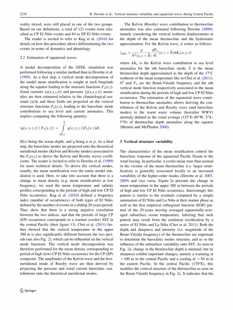
2009) and vice versa. Figure 2a presents the change in
mean temperature in the upper 300 m between the periods
of high and low CP El Nino occurrence. Interestingly this
pattern is similar to the residuals computed by a simple
summation of El Nino and La Nina at their mature phase as
well as the first empirical orthogonal function (EOF) pat-
tern of the 20-years moving averaged equatorially-aver-
aged subsurface ocean temperature, inferring that such
pattern may result from the nonlinear rectification by a
series of El Nino and La Nina (Choi et al. 2011). Both the
depth and sharpness and intensity (i.e. magnitude of the
Brunt-Vaisala frequency) of the thermocline are important
to determine the baroclinic modes structure, and as so the
influence of the subsurface variability onto SST. As seen in
Fig. 2a, change in the thermocline depth is minimal, but its
sharpness exhibit important changes, namely a warming at
*100 m in the central Pacific and a cooling at *50 m in
the eastern Pacific. In the central Pacific (170�E), this
modifies the vertical structure of the thermocline as seen on
the Brunt-Vaisala frequency in Fig. 2c. It indicates that the
2278 B. Dewitte et al.: Vertical structure variability and equatorial waves during Central Pacific
123
thermocline is less diffuse during periods of high CP El
Nino occurrence in the central Pacific, reflecting an
increase in stratification of *20% at the thermocline depth
compared to the periods of high EP El Nino occurrence
(Fig. 2c). In the meantime stratification decreases from the
surface to 100 m, reflecting that the Warm Pool is more
homogeneous. The change in mixed-layer depth (MLD) is
also indicative of the change in vertical structure variability
between the two mean states. The MLD is deeper by about
20 m in the central Pacific between the periods of high and
low CP El Nino occurrence [also shown in Choi et al.
(2011)]. Note that change in MLD mostly impacts the high-
order baroclinic modes (n [ 4), which can account for the
variability trapped in the surface layer due to their fine
vertical scales of variability.
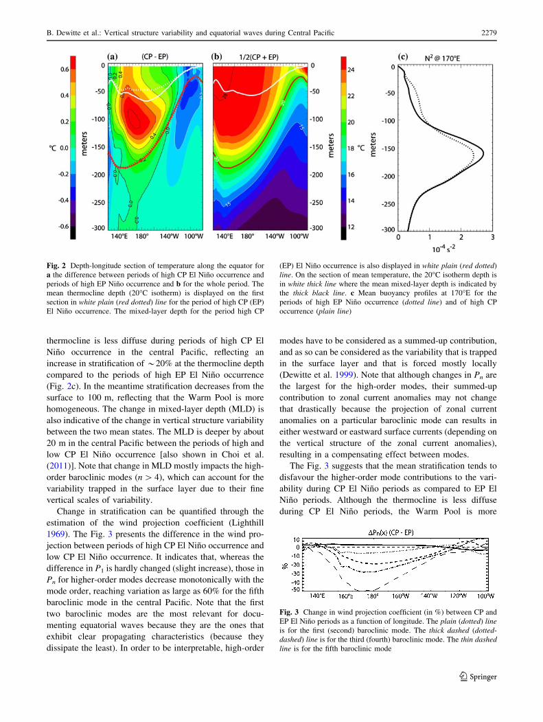
Change in stratification can be quantified through the
estimation of the wind projection coefficient (Lighthill
1969). The Fig. 3 presents the difference in the wind pro-
jection between periods of high CP El Nino occurrence and
low CP El Nino occurrence. It indicates that, whereas the
difference in P1 is hardly changed (slight increase), those in
Pn for higher-order modes decrease monotonically with the
mode order, reaching variation as large as 60% for the fifth
baroclinic mode in the central Pacific. Note that the first
two baroclinic modes are the most relevant for docu-
menting equatorial waves because they are the ones that
exhibit clear propagating characteristics (because they
dissipate the least). In order to be interpretable, high-order
modes have to be considered as a summed-up contribution,
and as so can be considered as the variability that is trapped
in the surface layer and that is forced mostly locally
(Dewitte et al. 1999). Note that although changes in Pn are
the largest for the high-order modes, their summed-up
contribution to zonal current anomalies may not change
that drastically because the projection of zonal current
anomalies on a particular baroclinic mode can results in
either westward or eastward surface currents (depending on
the vertical structure of the zonal current anomalies),
resulting in a compensating effect between modes.
The Fig. 3 suggests that the mean stratification tends to
disfavour the higher-order mode contributions to the vari-
ability during CP El Nino periods as compared to EP El
Nino periods. Although the thermocline is less diffuse
during CP El Nino periods, the Warm Pool is more
Fig. 2 Depth-longitude section of temperature along the equator for
a the difference between periods of high CP El Nino occurrence and
periods of high EP Nino occurrence and b for the whole period. The
mean thermocline depth (20�C isotherm) is displayed on the first
section in white plain (red dotted) line for the period of high CP (EP)
El Nino occurrence. The mixed-layer depth for the period high CP
(EP) El Nino occurrence is also displayed in white plain (red dotted)
line. On the section of mean temperature, the 20�C isotherm depth is
in white thick line where the mean mixed-layer depth is indicated by
the thick black line. c Mean buoyancy profiles at 170�E for the
periods of high EP Nino occurrence (dotted line) and of high CP
occurrence (plain line)
Fig. 3 Change in wind projection coefficient (in %) between CP and
EP El Nino periods as a function of longitude. The plain (dotted) lineis for the first (second) baroclinic mode. The thick dashed (dotted-
dashed) line is for the third (fourth) baroclinic mode. The thin dashedline is for the fifth baroclinic mode
B. Dewitte et al.: Vertical structure variability and equatorial waves during Central Pacific 2279
123

homogeneous (cf Fig. 2c) which overall leads to a reduced
projection of wind stress forcing onto the higher baroclinic
modes. Dynamically, this implies a tendency towards
ENSO related coupled instabilities having a faster propa-
gating speed (Dewitte 2000). The enhancement of the first
baroclinic mode relatively to the higher-order mode
favours an unstable mode having a fast westward propa-
gation and tends to increase the ENSO frequency (Dewitte
2000). This is because the suppression of higher-order
modes promotes the relative contribution of the zonal
advection feedback, which destabilizes Rossby waves. This
point will be got back to in Sect. 4.
As mentioned above, the inspection of the Pn is however
not sufficient to fully diagnose the relative contribution of
the baroclinic modes to the variability. Due to difference in
variability characteristics between the two events (Kug
et al. 2009), it is necessary to analyse the actual projection
of the variability onto the vertical mode functions. The
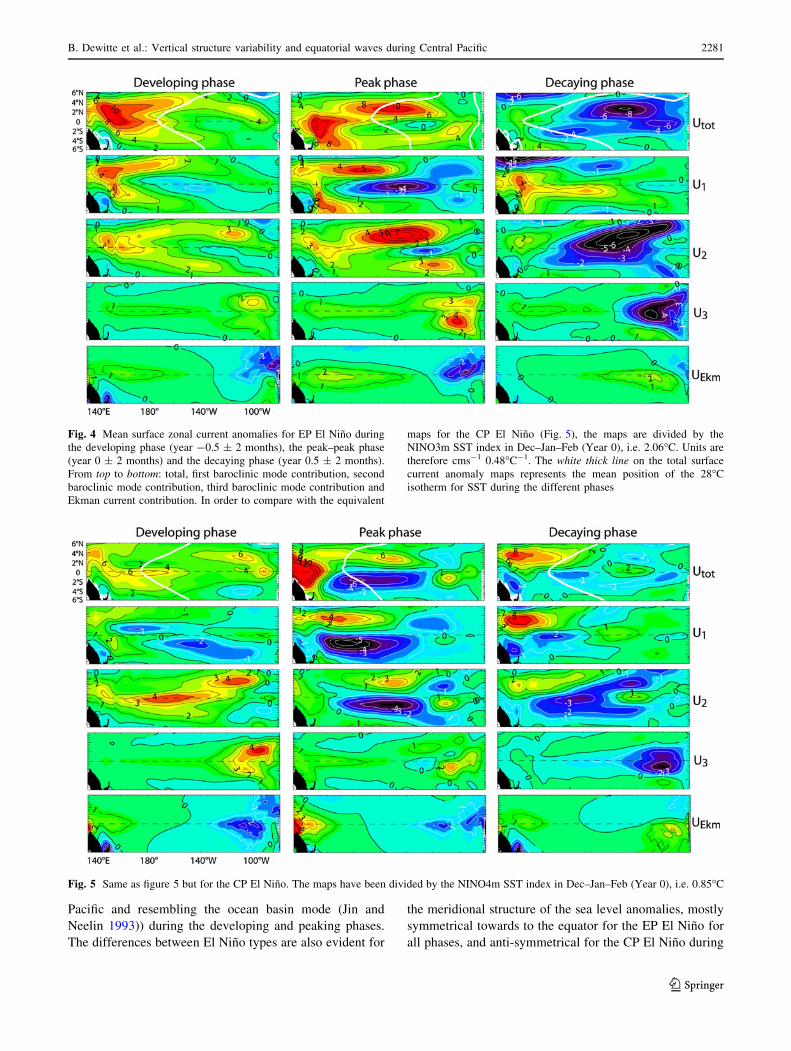
Fig. 4 provides such diagnostics for the zonal current
anomalies during the different phases of the events for the
EP El Nino composite. The peak phase corresponds to the
mean centred in January of year 1 within a 5-months
window (±2 months), the developing (decaying) phase is
centered 6 months before (after) the peak phase. Due to
difference in amplitude of the two type of El Nino, the
variability was divided by the NINO3m SST and NINO4m
SST anomaly index in Dec (Year 0) –Jan–Feb (Year 1)
respectively. In order to derive the contribution of the
summed-up contribution of the high-order modes (n [ 4),
relevant to the Ekman dynamics, a simple frictional
equation forced by s~f ¼ s~ 1hmix�P3
i¼1 Pi
� �is considered
following Blumenthal and Cane (1989) (Pi being the wind
projection coefficient for the baroclinic mode i and hmix is
the mixed-layer depth). The later represents the share of the
momentum flux that does not project on the gravest baro-
clinic modes (here, the first three baroclinic modes). This
leads to the estimation of zonal Ekman currents as:
uEkm ¼rssx þ bysy
q0ðr2s þ b2y2Þ
1
hmix
�X3
n¼1
Pn
!
where q0 is the mean density, rs is a damping rate coeffi-
cient of 1.5 days-1 and (sx, sy) is the zonal and meridional
wind stress anomalies.
The evolution of the total surface current anomaly
clearly illustrates the zonal advection process during EP El
Nino, namely eastward zonal current anomalies in the
vicinity of the eastern edge of the warm pool during the
developing and peak phases of the event. The decaying
phase is associated to strong westward surface currents
bringing back the warm pool westward. In terms of pro-
jection onto the baroclinic modes, the Fig. 4 indicates that
each mode has a different evolution, with the first mode
participating earlier than the other modes to the negative
feedback (westward equatorial current during the peak
phase). The strong reversal towards La Nina condition is
due to the contribution of modes 2 and 3 that exhibit
intense westward current during the decaying phase.
Ekman current anomalies have a westerly component in the
central Pacific during all phases, of which centre seems to
move eastward. An interesting aspect of the vertical mode
distribution is that the zonal current variability during the
reversal towards La Nina conditions takes place mostly
north of the equator through the second baroclinic mode.
This is consistent with the geostrophic adjustment con-
secutive to the discharge process (or ENSO-related
meridional mass transport) being larger in the Northern
Hemisphere than in the Southern Hemisphere during EP El
Nino (e.g. Kug et al. 2003). This is in contrast with the CP
El Nino as will be seen (Fig. 6).
Figure 5 presents the similar analysis to Fig. 4 but for
the CP El Nino composite. It indicates that the CP El Nino
has a different vertical mode distribution in terms of zonal
current anomalies than the EP El Nino, reflecting the dif-
ferences in time evolution. First of all, eastward zonal
current anomalies in the central-western Pacific during the
developing phase mostly project onto the second baroclinic
mode. Except during this phase, the baroclinic zonal cir-
culation is dominated by westward current anomalies in the
central and eastern Pacific, which actually lead to the
cooling SST tendency through the cold temperature
advection. The warming tendency is maintained through
the eastward Ekman current anomalies in the far western
Pacific during all phases. Interestingly, the negative feed-
back associated to the westward current anomalies take
place during the peak phase of the event, which is in
contrast with the EP El Nino composite. These westward
current anomalies project mostly onto the first two baro-
clinic modes and peak south of the equator. Note also the
westward current anomalies associated to the Ekman
component in the eastern Pacific is consistent with the
increase in trade winds during the period of high CP El
Nino occurrence (Choi et al. 2011).
In order to determine how the differences between El
Nino types reflect in the dynamic height, the Fig. 6 dis-
plays the results of the vertical mode decomposition in
terms of sea level anomaly contribution. Only the first two
baroclinic modes are presented because they are the most
relevant for the geostrophic basin scale adjustment asso-
ciated to wave dynamics. The results indicate that, whereas
the sea level pattern during EP El Nino is characterized by
a zonal seesaw reflecting the forcing of energetic eastern
Pacific Kelvin and western Pacific Rossby waves, the sea
level pattern during CP El Nino tends to have has a basin-
scale structure with positive sea level anomalies over most
of the equatorial Pacific (peaking in the central and western
2280 B. Dewitte et al.: Vertical structure variability and equatorial waves during Central Pacific
123
Pacific and resembling the ocean basin mode (Jin and
Neelin 1993)) during the developing and peaking phases.
The differences between El Nino types are also evident for
the meridional structure of the sea level anomalies, mostly
symmetrical towards to the equator for the EP El Nino for
all phases, and anti-symmetrical for the CP El Nino during
Fig. 4 Mean surface zonal current anomalies for EP El Nino during
the developing phase (year -0.5 ± 2 months), the peak–peak phase
(year 0 ± 2 months) and the decaying phase (year 0.5 ± 2 months).
From top to bottom: total, first baroclinic mode contribution, second
baroclinic mode contribution, third baroclinic mode contribution and
Ekman current contribution. In order to compare with the equivalent
maps for the CP El Nino (Fig. 5), the maps are divided by the
NINO3m SST index in Dec–Jan–Feb (Year 0), i.e. 2.06�C. Units are
therefore cms-1 0.48�C-1. The white thick line on the total surface
current anomaly maps represents the mean position of the 28�C
isotherm for SST during the different phases
Fig. 5 Same as figure 5 but for the CP El Nino. The maps have been divided by the NINO4m SST index in Dec–Jan–Feb (Year 0), i.e. 0.85�C
B. Dewitte et al.: Vertical structure variability and equatorial waves during Central Pacific 2281
123
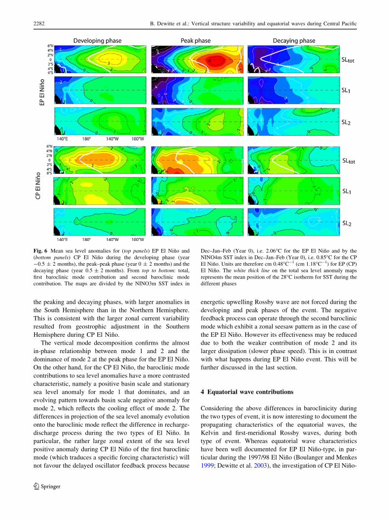
the peaking and decaying phases, with larger anomalies in
the South Hemisphere than in the Northern Hemisphere.
This is consistent with the larger zonal current variability
resulted from geostrophic adjustment in the Southern
Hemisphere during CP El Nino.
The vertical mode decomposition confirms the almost
in-phase relationship between mode 1 and 2 and the
dominance of mode 2 at the peak phase for the EP El Nino.
On the other hand, for the CP El Nino, the baroclinic mode
contributions to sea level anomalies have a more contrasted
characteristic, namely a positive basin scale and stationary
sea level anomaly for mode 1 that dominates, and an
evolving pattern towards basin scale negative anomaly for
mode 2, which reflects the cooling effect of mode 2. The
differences in projection of the sea level anomaly evolution
onto the baroclinic mode reflect the difference in recharge-
discharge process during the two types of El Nino. In
particular, the rather large zonal extent of the sea level
positive anomaly during CP El Nino of the first baroclinic
mode (which traduces a specific forcing characteristic) will
not favour the delayed oscillator feedback process because
energetic upwelling Rossby wave are not forced during the
developing and peak phases of the event. The negative
feedback process can operate through the second baroclinic
mode which exhibit a zonal seesaw pattern as in the case of
the EP El Nino. However its effectiveness may be reduced
due to both the weaker contribution of mode 2 and its
larger dissipation (slower phase speed). This is in contrast
with what happens during EP El Nino event. This will be
further discussed in the last section.
4 Equatorial wave contributions
Considering the above differences in baroclinicity during
the two types of event, it is now interesting to document the
propagating characteristics of the equatorial waves, the
Kelvin and first-meridional Rossby waves, during both
type of event. Whereas equatorial wave characteristics
have been well documented for EP El Nino-type, in par-
ticular during the 1997/98 El Nino (Boulanger and Menkes
1999; Dewitte et al. 2003), the investigation of CP El Nino-
Fig. 6 Mean sea level anomalies for (top panels) EP El Nino and
(bottom panels) CP El Nino during the developing phase (year
-0.5 ± 2 months), the peak–peak phase (year 0 ± 2 months) and the
decaying phase (year 0.5 ± 2 months). From top to bottom: total,
first baroclinic mode contribution and second baroclinic mode
contribution. The maps are divided by the NINO3m SST index in
Dec–Jan–Feb (Year 0), i.e. 2.06�C for the EP El Nino and by the
NINO4m SST index in Dec–Jan–Feb (Year 0), i.e. 0.85�C for the CP
El Nino. Units are therefore cm 0.48�C-1 (cm 1.18�C-1) for EP (CP)
El Nino. The white thick line on the total sea level anomaly maps
represents the mean position of the 28�C isotherm for SST during the
different phases
2282 B. Dewitte et al.: Vertical structure variability and equatorial waves during Central Pacific
123

type in terms of equatorial wave are very few (McPhaden
2004). The GFDL composite offers the opportunity to
reveal statistically significant features, which can be then
used to interpret observed events. As a benchmark, we
present the results of the horizontal mode decomposition
for the EP El Nino (Fig. 7). Results of Fig. 7 are consistent
with an earlier study that documented the wave sequence
according to the first two baroclinic mode during the
1997/1998 El Nino (Dewitte et al. 2003), indicating that the
characteristics of equatorial waves associated with EP El
Nino in the GFDL model are consistent with counterparts
of the observations. In particular, the EP El Nino is char-
acterized by a similar contribution and a quasi in-phase
relationship of the first and second baroclinic modes Kelvin
and Rossby waves, with the second baroclinic mode Kelvin
wave growing during the mature phase and leading to the
sharp reversal towards cool conditions through the reflec-
tion into Rossby wave at the eastern boundary [see Dewitte
et al. (2003)].
We now document the wave sequence during the CP El
Nino (Fig. 8). The developing phase is somewhat similar to
the one of the EP El Nino as the two downwelling (i.e.
positive) Kelvin modes work together to intensify SST
anomaly in the central Pacific, with however a dominant
contribution from mode 1 instead of mode 2. The marked
difference with the EP El Nino (Fig. 7) is the positive sign
of the Kelvin wave of the first baroclinic mode during the
decay phase, especially between Year 0 and Year ?1.
Therefore during CP events the first baroclinic mode is
mostly associated to downwelling (i.e. positive) Kelvin
wave over the whole cycle, which veils the delayed
oscillator (e.g. recharge-discharge) negative feedback pro-
cess. Whereas the first baroclinic mode is mostly associated
to downwelling (i.e. positive) Kelvin wave over the whole
cycle, the second baroclinic mode is dominated by the
upwelling (i.e. negative) Kelvin waves during the peak and
decaying phases, which may damp SST anomalies in the
central and eastern Pacific through vertical advection.
However in the decaying phase, the contributions by the
two Kelvin modes are opposite so the effects may be
compensated to each other. Another interesting feature is
the limited zonal extension of the Kelvin and Rossby
waves for the first baroclinic mode with peak variability in
the central Pacific. In particular, the first vertical mode
resembles the ocean basin mode (Jin and Neelin 1993;
Neelin and Jin 1993; Kang et al. 2004) such that the
maximum appears at the centre of the basin and the min-
imums (nodes) are located at the boundaries. This tends to
increase the contribution of the zonal advective feedback
(more intense in the central Pacific) with respect to the
thermocline feedback (more intense in the eastern Pacific)
in relation with equatorial wave variability. Therefore in
some sense, the CP El Nino may be related to the excite-
ment of the ocean basin mode, which is destabilized by the
zonal advective feedback. Propagating characteristics of
the Kelvin wave also suggest more intense modal disper-
sion in the eastern Pacific than during the EP El Nino. Note
for instance the sharp decay (amplification) of the down-
welling (upwelling) Kelvin wave amplitude of baroclinic
mode 1 (2) at *120�W. This is consistent with the fact that
the east–west contrast of stratification is more intense
during CP El Nino than during EP El Nino because the
Fig. 7 Time-longitude section of the equatorial Kelvin wave (AK in
cm) and the first meridional Rossby wave (R1 in cms-1) along the
equator for the (left) first and (right) second baroclinic modes during
EP El Nino event. R1 is displayed in reverse from 90�W to 135�E to
visualize wave reflections at eastern boundaries. Because R1 accounts
for currents and AK for sea level, they have opposite sign near the
boundaries. Contour intervals are 0.5 cm for AK and 5 cms-1 for R1.
The thick white line represents the position of the 28�C isotherm for
SST
B. Dewitte et al.: Vertical structure variability and equatorial waves during Central Pacific 2283
123

mean thermocline slope is hardly modified during the CP
El Nino. Furthermore, as mentioned in An and Jin (2000),
because the natural frequency of the ocean basin mode is
higher than the frequency of the ocean basin adjustment
mode, a shorter period of oscillation would be expected for
CP El Nino as compared to EP El Nino. Like for the EP El
Nino, the displacement of the eastern edge of the warm
pool mimics the pulses of downwelling Kelvin wave.
However the downwelling Kelvin wave slightly leads the
displacement of the warm pool edge, possibly because of
the delayed SST response to the vertical thermal advection
(Zelle et al. 2004).
The Fig. 9 further illustrates the peculiarities of the
Kevin wave according to the baroclinic modes during CP
El Nino contrasting with the EP El Nino. For the CP El
Nino in particular, it is obvious that only the second
baroclinic mode has a cooling effect during the decaying
phase. Such cooling effect is all the more important in the
eastern Pacific as the mean thermocline is shallower than
during EP El Nino. On the other hand, in the central
Pacific, since the thermocline is deeper than normal, the
effectiveness of the upwelling Kelvin/Rossby wave is
limited.
5 Discussion and conclusions
A long-term simulation of the GFDL_CM2.1 model was
used to document the variability characteristics of the CP
and EP El Nino in terms of equatorial wave. It is shown
that, despite a weaker variability than the EP El Nino, the
CP El Nino is associated to energetic first and second
baroclinic mode Kelvin and Rossby waves. Whereas for
the first baroclinic mode Kelvin wave have the maximum
amplitude at the centre of the basin and the minimum
amplitude (nodes) at the boundaries, resembling the ocean
basin mode (Jin and Neelin 1993; Neelin and Jin 1993;
Kang et al. 2004), the second baroclinic mode Kelvin wave
exhibits clearer free propagating characteristics resembling
the ocean adjustment mode of the EP El Nino (Jin 1997), In
particular, energetic upwelling Kelvin waves of the second
baroclinic mode are generated during the decaying phase of
the event, which maintains the east–west mean SST con-
trast across the Pacific, auspicious for the enhancement/
maintenance of the effectiveness of the zonal advective
feedback. This may explain the persistence/maintenance of
warm SST anomalies in the western Pacific during CP El
Nino. It also indicates that the reflective advective feed-
back process proposed by Picaut et al. (1996) cannot be
effective during CP El Nino events, basically because the
first baroclinic mode downwelling Kelvin waves has a
weak amplitude near the eastern boundary and because the
eastern edge of the warm pool remains in the central
Pacific. Similarly the delayed oscillator is not operating
during CP El Nino for the first baroclinic mode in the
GFDL model which may be attributed to the western most
position of the wind variability (Kug et al. 2010; cf.
Fig. 11). The wind stress forcing located near the western
boundary does not allow for accumulation of momentum
forcing towards the upwelling Rossby wave. In particular
wave reflection at the western boundary appears to be weak
(Fig. 8a, b), preventing negative feedback through the
reflected upwelling Kelvin wave. These differences in
negative feedback processes associated to wave dynamics
between El Nino types suggest that the recharge-discharge
process (Jin 1997) is operating differently during the two
type of El Nino. As a consistency check of this latter
statement, the WWV anomaly associated to the Kelvin and
Fig. 8 Same as Fig. 7 but for the CP El Nino event
2284 B. Dewitte et al.: Vertical structure variability and equatorial waves during Central Pacific
123

first-meridional Rossby waves was estimated (see Sect. 2).
Its evolution during the two types of El Nino is presented in
Fig. 10. Besides differences in amplitude (reflecting dif-
ferences in the magnitude of the events), the WWV has a
comparable evolution for both type of event, namely a
recharge prior to the maximum SST anomaly and a dis-
charge later on. However for the CP El Nino, the decrease
of the WWV anomaly is relatively weaker than for the EP
El Nino. The most striking difference between CP and EP
El Nino events is mainly in the role of the baroclinic
modes: For the EP El Nino, the WWV anomaly associated
to the first and second baroclinic modes has a comparable
evolution and amplitude. However for the CP El Nino, the
WWV anomaly of the first baroclinic mode is associated to
a recharge process during almost the whole cycle while the
WWV anomaly of the second baroclinic mode is associ-
ated to the discharge process after the peak SST anomaly.
This is consistent with the Kelvin wave decomposition of
the CP El Nino, which indicates that the first baroclinic
mode is associated to the warming of SST through
downwelling Kelvin wave, whereas the second baroclinic
modes tends to be associated to the cooling of SST (in
particular in the eastern equatorial Pacific) through
upwelling Kelvin wave that are all the more efficient that
the mean thermocline is shallower during periods of CP El
Nino occurrence.
The peculiarities of the Kelvin waves during the CP El
Nino event are more than likely resulting from the char-
acteristics of the zonal wind stress forcing, although they
could also result from non-linear processes such as modal
dispersion. In particular since the thermocline remains
shallow in the east during the CP El Nino and because
wave amplitude is weaker than during the EP El Nino, the
modal dispersion process associated to the east–west zonal
contrast in stratification can be operating effectively
(Busalacchi and Cane 1988). This is consistent with the
sharp decay of the downwelling Kelvin wave of the first
baroclinic mode around *120�W (Fig. 8a) and the relative
Fig. 9 Time evolution of the a, b Kelvin wave amplitude and
c, d thermocline depth (20�C isotherm depth) at 180� and 100�W.
Thick (thin) lines are for the CP (EP) El Nino. Dotted (plain) lines are
for the second (first) baroclinic modes. Kelvin wave amplitude
has been adimensionalized by its variability (RMS) between -0.5
and ?0.5 years
Fig. 10 Evolution of the a NINO3m and b NINO4m SST indices
(thick black lines) and Warm Water Volume (125�E–80�W; 5�S–5�N)
anomaly during the EP and CP El Ninos. The Warm Water Volume
considers the contribution of the Kelvin and first-meridional Rossby
wave of the first baroclinic mode (red dashed line), of the second
baroclinic mode (blue dashed line) and the summed-up contribution
of the first two modes (thick full red line)
B. Dewitte et al.: Vertical structure variability and equatorial waves during Central Pacific 2285
123
maximum at this longitude of the variability of the second
baroclinic mode Kelvin wave (Fig. 8c).
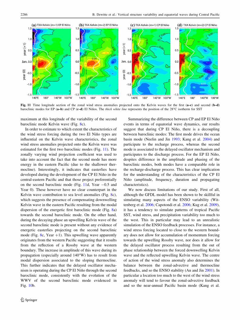
In order to estimate to which extent the characteristics of
the wind stress forcing during the two El Nino types are
influential on the Kelvin wave characteristics, the zonal
wind stress anomalies projected onto the Kelvin wave was
estimated for the first two baroclinic modes (Fig. 11). The
zonally varying wind projection coefficient was used to
take into account the fact that the second mode has more
energy in the eastern Pacific (due to the shallower ther-
mocline). Interestingly, it indicates that easterlies have
developed during the development of the CP El Nino in the
central-eastern Pacific and that those project preferentially
on the second baroclinic mode (Fig. 11d, Year -0.5 and
Year 0). These however have no clear counterpart in the
Kelvin wave contribution to sea level anomalies (Fig. 8c),
which suggests the presence of compensating downwelling
Kelvin wave in the eastern Pacific resulting from the modal
dispersion of the energetic first baroclinic mode (Fig. 8a)
towards the second baroclinic mode. On the other hand,
during the decaying phase an upwelling Kelvin wave of the
second baroclinic mode is present without any evidence of
energetic easterlies projecting on the second baroclinic
mode (Fig. 8c, Year ?1). This upwelling wave apparently
originates from the western Pacific suggesting that it results
from the reflection of a Rossby wave at the western
boundary. The increase in amplitude of this wave during its
propagation (especially around 140�W) has to result from
modal dispersion associated to the sloping thermocline.
This further indicates that the delayed oscillator mecha-
nism is operating during the CP El Nino through the second
baroclinic mode, consistently with the evolution of the
WWV of the second baroclinic mode evidenced in
Fig. 10b.
Summarizing the difference between CP and EP El Nino
events in terms of equatorial wave dynamics, our results
suggest that during CP El Nino, there is a decoupling
between baroclinic modes: The first mode drives the ocean
basin mode (Neelin and Jin 1993; Kang et al. 2004) and
participate to the recharge process, whereas the second
mode is associated to the delayed oscillator mechanism and
participates to the discharge process. For the EP El Nino,
despites difference in the amplitude and phasing of the
baroclinic modes, both modes have a comparable role in
the recharge-discharge process. This has clear implication
for the understanding of the characteristics of the CP El
Nino (amplitude, frequency, duration and propagating
characteristics).
We now discuss limitations of our study. First of all,
although the GFDL model has been shown to be skillful in
simulating many aspects of the ENSO variability (Wit-
tenberg et al. 2006; Capotondi et al. 2006; Kug et al. 2009),
it has a tendency to simulate patterns of tropical Pacific
SST, wind stress, and precipitation variability too much to
the west. This in particular may lead to an unrealistic
simulation of the ENSO feedback processes. For instance, a
wind stress forcing located to close to the western bound-
ary does not allow for accumulation of momentum forcing
towards the upwelling Rossby wave, nor does it allow for
the delayed oscillator process resulting from the out of
phase relationship between the forced downwelling Kelvin
wave and the reflected upwelling Kelvin wave. The centre
of action of the wind stress anomaly also determines the
balance between the zonal-advective and thermocline
feedbacks, and so the ENSO stability (An and Jin 2001). In
particular a location too much to the west of the wind stress
anomaly will tend to favour the zonal-advective feedback
and so the near-annual Pacific basin mode (Kang et al.
Fig. 11 Time longitude section of the zonal wind stress anomalies projected onto the Kelvin waves for the first (a–c) and second (b–d)
baroclinic modes for EP (a–b) and CP (c–d) El Ninos. The thick white line represents the position of the 28�C isotherm for SST
2286 B. Dewitte et al.: Vertical structure variability and equatorial waves during Central Pacific
123
2004). This is consistent with the results of the wave
decomposition which clearly shows the basin mode nature
of the first baroclinic mode during periods of high CP El
Nino (Fig. 8a). In the observations, the wind stress anom-
aly associated to ENSO is not as much to the west as in the
GFDL model. However, during observed CP El Ninos, it is
somewhat *10� to the west of that during EP El Ninos and
does not extent as much to the east (not shown). This has
the potential to modify the balance between the feedback
processes in a way that may also favour the near-annual
Pacific basin mode. Nevertheless composite analysis based
on the new ocean reanalysis (SODA) that covers the period
from 1871 to 2008 (Giese and Ray 2011) does not reveal a
contrasted behaviour between both type of El Nino in terms
of their vertical structure variability. The SODA CP com-
posite1 for the first baroclinic mode do exhibit pulses of
downwelling Kelvin wave peaking in the central Pacific
and having decaying amplitude near the boundaries remi-
niscent of the ocean basin mode (not shown). However
both baroclinic modes are characterized by a clear reversal
from warm to cold indicating that they have comparable
behaviour of the discharge process, conversely to the
GFDL CP composite. It is difficult here to draw firm
conclusions from the SODA composite due to the sensi-
tivity of the results to the number of event that are retained.
It is clear that there is a larger diversity of the evolution of
the events in the SODA Reanalysis compared to the GFDL
model, which somehow limits any generalisation. In par-
ticular, Kug et al. (2009) introduced three types of El Nino,
i.e. CP, EP, and a mixed type. For instance, the last El Nino
to date that took place in 2009–2010 can be categorized as
a CP El Nino (Kim et al. 2011) but its ocean dynamical
behavior resembles the EP El Nino. Yu et al. (2011) also
propose to define CP El Nino and mixed-type El Nino
based on subsurface indices that are more appropriate to
capture the specificities of the events and account for the
larger diversity of the El Nino types in nature than what is
simulated in the GFDL model. Noteworthy the GFDL
model is also characterized by a clear relationship between
mean state and CP El Nino occurrence (Choi et al. 2011)
which is not evidenced from the SODA reanalysis. In fact,
the increased occurrence of the CP El Nino occurs under a
warmer mean state in the central Pacific in the GFDL
model, which somehow is comparable to the situation in
the recent decade (Takahashi et al. 2011; McPhaden et al.
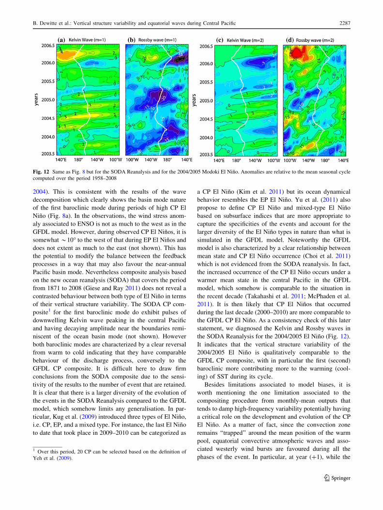
2011). It is then likely that CP El Ninos that occurred
during the last decade (2000–2010) are more comparable to
the GFDL CP El Nino. As a consistency check of this later
statement, we diagnosed the Kelvin and Rossby waves in
the SODA Reanalysis for the 2004/2005 El Nino (Fig. 12).
It indicates that the vertical structure variability of the
2004/2005 El Nino is qualitatively comparable to the
GFDL CP composite, with in particular the first (second)
baroclinic more contributing more to the warming (cool-
ing) of SST during its cycle.
Besides limitations associated to model biases, it is
worth mentioning the one limitation associated to the
compositing procedure from monthly-mean outputs that
tends to damp high-frequency variability potentially having
a critical role on the development and evolution of the CP
El Nino. As a matter of fact, since the convection zone
remains ‘‘trapped’’ around the mean position of the warm
pool, equatorial convective atmospheric waves and asso-
ciated westerly wind bursts are favoured during all the
phases of the event. In particular, at year (?1), while the
1 Over this period, 20 CP can be selected based on the definition of
Yeh et al. (2009).
Fig. 12 Same as Fig. 8 but for the SODA Reanalysis and for the 2004/2005 Modoki El Nino. Anomalies are relative to the mean seasonal cycle
computed over the period 1958–2008
B. Dewitte et al.: Vertical structure variability and equatorial waves during Central Pacific 2287
123
EP El Nino event starts its decaying phase (and its reversal
to cool conditions), the warm conditions during the CP El
Nino can be maintained by the convective equatorial wave
activity at the consecutive peak season (March–April–
May). This stresses on the likely stronger coupling between
tropical intraseasonal atmospheric variability and ENSO
during the CP El Nino than during the EP El Nino. Current
efforts are devoted to the investigation of such aspect of the
CP and EP El Nino variability.
Acknowledgments S.-I. An was supported by the National
Research Foundation of Korea (NRF) grant funded by the Korea
government (MEST) (No. 2011-0015208). Sulian Thual benefited
from support of the CNRS (Centre National de la Recherche Scien-
tifique) through a STAR (Science and Technology Amicable
Research) program (No. 25848VL). The two anonymous reviewers
are thanked for their constructive comments.
References
An S-I, Jin F–F (2000) An eigen analysis of the interdecadal changes
in the structure and frequency of ENSO mode. Geophys Res Lett
27:1573–1576
An S-I, Jin F–F (2001) Collective role of thermocline and zonal
advective feedbacks in the ENSO mode. J Clim 14:3421–3432
Ashok K, Behera SK, Rao SA, Weng H, Yamagata T (2007) El Nino
Modoki and its possible teleconnection. J Geophys Res
112:C11007
Bejarano L, Jin F–F (2008) Coexistence of equatorial coupled modes
of ENSO. J Clim 21:3051–3067
Blumenthal B, Cane MA (1989) Accounting for parameter uncer-
tainties in model verification: an illustration with tropical sea
surface temperature. J Phys Oceanogr 19:815–830
Boulanger J-P, Menkes C (1999) Long equatorial wave reflection in
the Pacific Ocean during the 1992–1998 TOPEX/POSEIDON
period. Clim Dyn 15:205–225
Busalacchi AJ, Cane MA (1988) The effect of varying stratification
on low-frequency equatorial motions. J Phys Oceanogr
18(6):801–812
Capotondi A, Wittenberg A, Masina S (2006) Spatial and temporal
structure of tropical Pacific interannual variability in 20th
century coupled simulations. Ocean Model 15:274–298
Carton JA, Giese BS (2008) A reanalysis of ocean climate using
simple ocean data assimilation (SODA). Month Weath Rev
136(8):2999–3017
Choi J, An S-I, Kug J-S, Yeh S-W (2011) The role of mean state on
changes in El Nino’s flavours. Clim Dyn 37:1205–1215
Cravatte S, Delcroix T, Zhang D, McPhaden M, Leloup J (2009)
Observed freshening and warming of the western Pacific warm
pool. Clim Dyn 33:565–589. doi:10.1007/s00382-009-0526-7
Delworth TL et al (2006) GFDL’s CM2 global coupled climate
models. Part I: formulation and simulation characteristics. J Clim
19:634–674
Dewitte B (2000) Sensitivity of an intermediate coupled ocean-
atmosphere model of the tropical Pacific to its oceanic vertical
structure. J Clim 13:2363–2388
Dewitte B, Reverdin G, Maes C (1999) Vertical structure of an
OGCM simulation of the equatorial Pacific Ocean in 1985–1994.
J Phys Oceanogr 29:1542–1570
Dewitte B, Illig S, Parent L, duPenhoat Y, Gourdeau L, Verron J
(2003) Tropical Pacific baroclinic mode contribution and
associated long waves for the 1994–1999 period from an
assimilation experiment with altimetric data. J Geophys Res
108(C4):3121–3138
Dewitte B, Yeh S-W, Moon B-K, Cibot C, Terray L (2007)
Rectification of the ENSO variability by interdecadal changes
in the equatorial background mean state in a CGCM simulation.
J Climate 20(10):2002–2021
Dewitte B, Thual S, Yeh S-W, An S-I, Moon B-K, Giese B (2009)
Low frequency variability of temperature in the vicinity of the
equatorial thermocline in SODA: role of equatorial wave
dynamics and ENSO asymmetry. J Climate 22:5783–5795
Giese B, Ray S (2011) El Nino variability in simple ocean data
assimilation (SODA):1871–2008. J Geophys Res 116:C02024.
doi:10.1029/2010JC006695
Gnanadesikan A et al (2006) GFDL’s CM2 global coupled climate
models, Part II: the baseline ocean simulation. J Clim
19:675–697
Griffies SM et al (2005) Formulation of an ocean model for global
climate simulations. Ocean Sci 1:45–79
Jin FF (1997) An equatorial ocean recharge paradigm for ENSO. Part
I: conceptual model. J Atmos Sci 54:811–829
Jin F–F, Neelin JD (1993) Modes of interannual tropical ocean-
atmosphere interaction—a unified view. Part I: numerical results.
J Atmos Sci 50:3477–3503
Jin F-F, Kug JS, An S-I, Kang IS (2003) A near-annual coupled
ocean-atmosphere mode in the equatorial Pacific Ocean. Geo-
phys Res Lett 30:1080. doi:10.1029/2002GL015983
Kang I-S, Kug J-S, An S-I, Jin F–F (2004) A near-annual Pacific
Ocean Basin mode. J Clim 17:2478–2488
Kao H-Y, Yu J-Y (2009) Contrasting Eastern-Pacific and Central-
Pacific types of ENSO. J Clim 22:615–632
Kim W, Yeh S-W, Kim J-H, Kug J-S, Kwon M (2011) The unique
2009–2010 El Nino event: a fast phase transition of warm pool
El Nino to La Nina. Geophys Res Lett 38:L15809. doi:
10.1029/2011GL048521
Kug J-S, Kang I-S, An S-I (2003) Symmetric and asymmetric mass
exchanges between the equatorial and off-equatorial Pacific
associated with ENSO. J Geophys Res 108(NO. C8):3284. doi:
10.1029/2002JC001671
Kug J-S, Jin F–F, An S-I (2009) Two-types of El Nino events: cold
Tongue El Nino and Warm Pool El Nino. J Clim 22:1499–1515
Kug J-S, Choi J, An S-I, Jin F–F, Wittenberg A-T (2010) Warm pool
and cold tongue El Nino events as simulated by the GFDL2.1
coupled GCM. J Clim 23:1226–1239
Larkin NK, Harrison DE (2005a) On the definition of El Nino and
associated seasonal average U.S. weather anomalies. Geophys
Res Lett 32:L13705
Larkin NK, Harrison DE (2005b) Global seasonal temperature and
precipitation anomalies during El Nino autumn and winter.
Geophys Res Lett 32:L16705
Lee T, McPhaden M (2010) Increasing intensity of El Nino in the
central-equatorial Pacific. Geophys Res Lett 37:L14603. doi:
10.1029/2010GL044007
Lighthill MJ (1969) Dynamical response of the Indian Ocean to onset
of the southwest monsoon. Phil Trans R Soc A 265:45–92
Lin S-J (2004) A ‘‘vertically Lagrangian’’ finite-volume dynamical
core for global models. Mon Wea Rev 132:2293–2307
McPhaden MJ (2004) Evolution of the 2002–03 El Nino. Bull Am
Meteor Soc 85:677–695
McPhaden MJ, Busalacchi AJ, Cheney R, Donguy JR, Gage KS,
Halpern D, Ji M, Julian P, Meyers G, Mitchum GT, Niiler PP,
Picaut J, Reynolds RW, Smith N, Takeuchi K (1998) The
tropical ocean-global atmosphere (TOGA) observing system: a
decade of progress. J Geophys Res 103:14169–14240
McPhaden MJ, Lee T, McClurg D (2011) El Nino and its relationship
to changing background conditions in the tropical Pacific Ocean.
Geophys Res Lett 38:L15709. doi:10.1029/2011GL048275
2288 B. Dewitte et al.: Vertical structure variability and equatorial waves during Central Pacific
123

Meinen CS, McPhaden MJ (2000) Observations of warm water
volume changes in the equatorial Pacific and their relationship to
El Nino and La Nina. J Clim 13:3551–3559
Neelin JD, Jin F–F (1993) Modes of interannual tropical ocean–
atmosphere interaction—a unified view. Part II: analytical results
in the weak-coupling limit. J Atmos Sci 50:3504–3522
Neelin JD, Battisti DS, Hirst AC, Jin F–F, Wakata Y, Yamagata T,
Zebiak SE (1998) ENSO theory. J Geophy Res Oceans
103:14261–14290
Picaut J, Ioualalen M, Menkes C, Delcroix T, McPhaden MJ (1996)
Mechanism of the Zonal displacements of the pacific warm pool:
implications for ENSO. Science 274:1486–1489
Schopf P-S, Suarez M-J (1988) Vacillations in a coupled ocean-
atmosphere model. J Atmos Sci 45:549–566
Suarez MJ, Schopf PS (1989) A delayed action oscillator for ENSO.
J Atmos Sci 45:3283–3287
Takahashi K, Montecinos A, Goubanova K, Dewitte B (2011)
ENSO regimes: reinterpreting the canonical and Modoki El
Nino. Geophys Res Lett 38:L10704. doi:10.1029/2011GL
047364
Weng H, Ashok K, Behera S, Rao S, Yamagata T (2007) Impacts of
recent El Nino Modoki on dry/wet conditions in the Pacific Rim
during boreal summer. Clim Dyn 29:113–129
Wittenberg A, Rosati TA, Lau N-C, Ploshay JJ (2006) GFDL’s CM2
global coupled climate models. Part III: tropical Pacific climate
and ENSO. J Clim 19:698–722
Yeh S-W, Kug S-J, Dewitte B, Kwon M-H, Kirtman BP, Jin F–F
(2009) El Nino in a changing climate. Nature 461:511–514
Yu J-Y, Kim ST (2010a) Three evolution patterns of Central-Pacific El
Nino. Geophys Res Lett 37:L08706. doi:10.1029/2010GL042810
Yu J-Y, Kim ST (2010b) Identification of Central-Pacific and
Eastern-Pacific types of ENSO in CMIP3 models. Geophys
Res Lett 37. doi:10.1029/2010GL044082
Yu J-Y, Kim ST (2011) Relationships between extratropical sea level
pressure variations and the Central Pacific and Eastern Pacific
types of ENSO. J Clim 24:708–720
Yu J-Y, Kao H-Y, Lee T (2010) Subtropics-related interannual sea
surface temperature variability in the central equatorial Pacific.
J Clim 23:2869–2884
Yu J-Y, Kao H-Y, Lee T, Kim S (2011) Subsurface ocean
temperature indices for Central-Pacific and Eastern-Pacific types
of El Nino and La Nina events. Theoretical Appl Climatol
103:337–344
Zelle H, Appeldoorn G, Burgers G, van Oldenborgh GJ (2004) The
relationship between sea surface temperature and thermocline
depth in the eastern equatorial Pacific. J Clim 34:643–655
B. Dewitte et al.: Vertical structure variability and equatorial waves during Central Pacific 2289
123