VERMONT AGENCY OF TRANSPORTATION

Materials & Research Section Research Report

STATISTICAL ANALYSIS OF WEIGH-IN- MOTION DATA FOR BRIDGE DESIGN

IN VERMONT

Report 2014 – 14

December 2014

STATISTICAL ANALYSIS OF WEIGH-IN- MOTION DATA FOR BRIDGE DESIGN

IN VERMONT

Report 2014 – 14

DECEMBER 2014

Reporting on SPR-RAC-729

STATE OF VERMONT

AGENCY OF TRANSPORTATION

RESEARCH & DEVELOPMENT SECTION

BRIAN R. SEARLES, SECRETARY OF TRANSPORTATION

CHRIS COLE, DIRECTOR OF POLICY, PLANNING AND INTERMODAL DEVELOPMENT

JOE SEGALE, P.E./PTP, PLANNING, POLICY & RESEARCH

WILLIAM E. AHEARN, P.E., RESEARCH & DEVELOPMENT

Prepared By:

University of Vermont, Transportation Research Center

Eric M. Hernandez, Ph.D., Assistant Professor, School of Engineering

Transportation Research Center Farrell Hall

210 Colchester Avenue

Burlington, VT 05405

Phone: (802) 656-1312

Website: www.uvm.edu/transportationcenter

II

The information contained in this report was compiled for the use of the Vermont Agency

of Transportation (VTrans). Conclusions and recommendations contained herein are based upon

the research data obtained and the expertise of the researchers, and are not necessarily to be

construed as Agency policy. This report does not constitute a standard, specification, or

regulation. VTrans assumes no liability for its contents or the use thereof.

III

Technical Report Documentation Page

1. Report No. 2. Government Accession No. 3. Recipient's Catalog No. 2014-05 - - - - - -

4. Title and Subtitle 5. Report Date

STATISTICAL ANALYSIS OF WEIGH-IN-MOTION DATA FOR BRIDGE DESIGN IN VERMONT

October 2014 6. Performing Organization Code

7. Author(s) 8. Performing Organization Report No. Eric M. Hernandez, Assistant Professor, School of Engineering 2014-09 9. Performing Organization Name and Address 10. Work Unit No.

UVM Transportation Research Center Farrell Hall] 210 Colchester Avenue Burlington, VT 05405

11. Contract or Grant No.

RSCH017-729

12. Sponsoring Agency Name and Address 13. Type of Report and Period Covered

Vermont Agency of Transportation Materials and Research Section 1 National Life Drive National Life Building Montpelier, VT 05633-5001

Federal Highway Administration Division Office Federal Building Montpelier, VT 05602

Final 2012 – 2014

14. Sponsoring Agency Code

15. Supplementary Notes

16. Abstract This study investigates the suitability of the HL-93 live load model recommended by AASHTO LRFD Specifications for its use in the analysis and design of bridges in Vermont. The method of approach consists in performing a statistical analysis of weigh-in-motion (WIM) data collected between the years 2000-2012 at 12 stations across the state of Vermont. In total 36,754,819 individual WIM events were analyzed in this study. We compared the statistics of the lane moment and shear induced by the WIM data to the corresponding lane moment and shear induced by the HL-93 live load model. This analysis was performed on two types of very common bridge decks: (i) steel girders and concrete slabs and (ii) concrete girders with concrete slabs. In all cases the decks were considered to be acting fully composite. We considered span lengths in the range of 5-60 meters (~ 16-200 ft). The mains findings of this study are: (i) The probability that the lane moment and shear induced by the WIM data exceeds the corresponding values induced by the HL-93 model, decreases with span length. Averaged over all years considered in this study, the largest probability of exceedance was found to be approximately 1%. (ii) For span lengths exceeding 10 m, the annual probability of failure induced by the WIM data analysis did not exceed the annualized AASHTO target probability of failure. This indicates that for typical bridge decks with span length exceeding 10 meters, the HL-93 live load model is adequate for its use in Vermont. (iii) We propose that a more detailed study be carried out for short span structures such as culverts. Evidence from our study suggests that for very short spans (< 10 m), the HL-93 live load model might not be conservative.

17. Key Words 18. Distribution Statement

Statistical Analysis, Weigh-in-Motion, Bridge Design, LRFD, No Restrictions.

19. Security Classif. (of this report) 20. Security Classif. (of this page) 21. No. Pages 22. Price

- - - - - - - - - Form DOT F1700.7 (8-72) Reproduction of completed pages authorized

AcknowledgementsThe author would like to acknowledge funding from the Vermont Agency

of Transportation and the USDOT thru the University Transportation Center(UTC) program at the University of Vermont.

DisclaimerThe contents of this report reflect the views of the authors, who are

responsible for the facts and the accuracy of the data presented herein. Thecontents do not necessarily reflect the official view or policies of the Universityof Vermont. This report does not constitute a standard, specification, orregulation.

ABSTRACT

This study investigates the suitability of the HL-93 live load model recommended by AASHTO LRFD

Specifications for its use in the analysis and design of bridges in Vermont. The method of approach

consists in performing a statistical analysis of weigh-in-motion (WIM) data collected between the years

2000-2012 at 12 stations across the state of Vermont. In total 36,754,819 individual WIM events were

analyzed in this study. We compared the statistics of the lane moment and shear induced by the WIM data

to the corresponding lane moment and shear induced by the HL-93 live load model. This analysis was

performed on two types of very common bridge decks: (i) steel girders and concrete slabs and (ii)

concrete girders with concrete slabs. In all cases the decks were considered to be acting fully composite.

We considered span lengths in the range of 5-60 meters (~ 16-200 ft). The mains findings of this study

are: (i) The probability that the lane moment and shear induced by the WIM data exceeds the

corresponding values induced by the HL-93 model, decreases with span length. Averaged over all years

considered in this study, the largest probability of exceedance was found to be approximately 1%. (ii) For

span lengths exceeding 10 m, the annual probability of failure induced by the WIM data analysis did not

exceed the annualized AASHTO target probability of failure. This indicates that for typical bridge decks

with span length exceeding 10 meters, the HL-93 live load model is adequate for its use in Vermont. (iii)

We propose that a more detailed study be carried out for short span structures such as culverts. Evidence

from our study suggests that for very short spans (< 10 m), the HL-93 live load model might not be

conservative.

EXECUTIVE SUMMARY

This study investigates the suitability of the HL-93 live load model recommended by AASHTO LRFD

Specifications for its use in the analysis and design of bridges in Vermont. The method of approach

consists in performing a statistical analysis of weigh-in-motion (WIM) data collected between the years

2000-2012 at 12 stations across the state of Vermont. In total 36,754,819 individual WIM events were

analyzed in this study. The statistics of the lane moment and shear induced by the WIM data was

compared with the corresponding lane moment and shear induced by the HL-93 live load model. This

analysis was performed on two types of very common bridge decks: (i) steel girders and concrete slabs

and (ii) concrete girders with concrete slabs. In all cases, the decks were considered to be acting fully

composite. Span lengths in the range of 5-60 meters (~ 16-200 ft) were considered. As a general trend it

was found that as the span length increases, the probability that the lane moment and shear induced by the

WIM data exceeds the values induced by the HL-93 model, decreases. Averaged over all years considered

in this study, the largest probability of exceedance was found to be approximately 1%, this occurred in 5

meter spans. The largest probability of exceedance in any single year and station was found to be 2.5%,

again for 5 meters span lengths.

In terms of structural reliability, an analysis that included the variability in loading (using the statistical

analysis of WIM data) and the variability in strength of the bridge deck (using values from the literature)

were performed. This analysis was done for steel girder and concrete slab decks for span lengths in the

range of 10-60 meters (~ 16-200ft). The results were compared with the AASHTO LRFD target reliability

index of 3.5 in 75 years (probability of failure of 0.023% in 75 years). In this analysis it was found that

the annual probability of failure induced by the WIM data analysis did not exceed the annualized

AASHTO target probability of failure. This indicates that for typical bridge decks with span length

exceeding 10 meters, the HL-93 live load model is adequate for its use in Vermont.

Based on our statistical analysis of the available WIM data and the subsequent reliability analysis, it is

proposed that a more detailed study be carried out for short span structures such as culverts. Evidence

from our study suggests that for very short spans (< 10 m), the HL-93 live load model might not be

conservative, in the sense that it is not consistent with the target reliability index of 3.5 in 75 years. This

requires a separate study since culverts have a different type of structural system in comparison with

typical bridge decks.

Contents

1 Introduction 121.1 History of Design Codes . . . . . . . . . . . . . . . . . . . . . 121.2 Probabilistic Design vs. Allowable Stress Design . . . . . . . . 141.3 Evaluation of Live Load Model in AASHTO LRFD . . . . . . 16

2 Literature Review 192.1 NCHRP Report 368: Calibration of LRFD Bridge Design Code 192.2 Characteristic Traffic Load Effects from a Mixture of Loading

Events on Short to Medium Span Bridges . . . . . . . . . . . 212.3 Probabilistic Characterization of Live Load Using Visual Counts

and In-Service Strain Monitoring . . . . . . . . . . . . . . . . 222.4 WIM Based Live Load Model for Bridge Reliability . . . . . . 232.5 Calibration of Live-Load Factor in LRFD Bridge Design Spec-

ifications Based on State-Specific Traffic Environments . . . . 232.6 Using Weigh-In-Motion Data to Determine Aggressiveness of

Traffic for Bridge Loading . . . . . . . . . . . . . . . . . . . . 242.7 Reliability of Highway Girder Bridges . . . . . . . . . . . . . . 252.8 Locality of Truck Loads and Adequacy of Bridge Design Load 252.9 Buckling Reliability of Deteriorating Steel Beam Ends . . . . . 262.10 Evaluation of a Permit Vehicle Model Using Weigh-In-Motion

Truck Records . . . . . . . . . . . . . . . . . . . . . . . . . . . 262.11 Applying Weigh-In-Motion Traffic Data to Reliability Based

Assessment of Bridge Structures . . . . . . . . . . . . . . . . . 272.12 Site Specific Probability Distribution of Extreme Traffic Ac-

tion Effects . . . . . . . . . . . . . . . . . . . . . . . . . . . . 272.13 Monte Carlo Simulation of Extreme Traffic Loading on Short

and Medium Span Bridges . . . . . . . . . . . . . . . . . . . . 28

3

2.14 Information Regarding WIM Data Sets Used in Reviewed Stud-ies . . . . . . . . . . . . . . . . . . . . . . . . . . . . . . . . . 29

3 Identification of Mixture Models from Weigh-in-Motion Datawith Application to Bridge Deck Reliability Analysis 303.1 Introduction . . . . . . . . . . . . . . . . . . . . . . . . . . . . 313.2 AASHTO Live Load Model . . . . . . . . . . . . . . . . . . . 333.3 Description of Data and Pre-Processing . . . . . . . . . . . . . 343.4 Statistical Analysis Methods . . . . . . . . . . . . . . . . . . . 36

3.4.1 Mixture Models . . . . . . . . . . . . . . . . . . . . . . 363.4.2 Expectation Maximization Algorithm . . . . . . . . . . 37

3.5 Results . . . . . . . . . . . . . . . . . . . . . . . . . . . . . . . 373.5.1 Spatial Variability . . . . . . . . . . . . . . . . . . . . 383.5.2 Temporal Variability . . . . . . . . . . . . . . . . . . . 38

3.6 Reliability Analysis . . . . . . . . . . . . . . . . . . . . . . . . 393.7 Conclusions and Future Work . . . . . . . . . . . . . . . . . . 403.8 Acknowledgement . . . . . . . . . . . . . . . . . . . . . . . . . 413.9 Figures . . . . . . . . . . . . . . . . . . . . . . . . . . . . . . . 41

4 Bayesian Model Averaging Methods for Identifying Live LoadStress Demand Extreme Value Distributions in Bridges 554.1 Introduction . . . . . . . . . . . . . . . . . . . . . . . . . . . . 554.2 The Data . . . . . . . . . . . . . . . . . . . . . . . . . . . . . 574.3 Extreme Value Theory . . . . . . . . . . . . . . . . . . . . . . 584.4 Daily Maximum Bending Moments and Extreme Value Theory 594.5 Probability Models . . . . . . . . . . . . . . . . . . . . . . . . 60

4.5.1 Normal Models . . . . . . . . . . . . . . . . . . . . . . 604.5.2 GEV Models . . . . . . . . . . . . . . . . . . . . . . . 604.5.3 Gamma Model . . . . . . . . . . . . . . . . . . . . . . 62

4.6 Bayesian Parameter Estimation . . . . . . . . . . . . . . . . . 624.7 Evaluation of Probability Models . . . . . . . . . . . . . . . . 65

4.7.1 Chi-Square test . . . . . . . . . . . . . . . . . . . . . . 654.7.2 Bayesian Model Averaging . . . . . . . . . . . . . . . . 66

4.8 Results . . . . . . . . . . . . . . . . . . . . . . . . . . . . . . . 684.9 Conclusion . . . . . . . . . . . . . . . . . . . . . . . . . . . . . 704.10 Figures . . . . . . . . . . . . . . . . . . . . . . . . . . . . . . . 70

Appendices 85

4

A Axle Statistics by Station 86

B Cross Sections of Superstructures Designed using AASHTOLRFD 99

C Bridge Finite Element Models 101

D Fit of Mixture Models to Data 104

5

List of Figures

1.1 Concept of Probabilistic Design . . . . . . . . . . . . . . . . . 151.2 Normally Distributed Loads and Resistance . . . . . . . . . . 16

3.1 AASHTO HL-93 live load model per lane of traffic. . . . . . . 413.2 Geographical location and designation of WIM stations in Ver-

mont. . . . . . . . . . . . . . . . . . . . . . . . . . . . . . . . 423.3 Total number of measured vehicles per year in all WIM stations 423.4 Illustration of a potential axle location within a simply sup-

ported span. . . . . . . . . . . . . . . . . . . . . . . . . . . . . 433.5 Proportion of measured vehicles that generate moments and(or)

shears that exceed HL-93 induced moments and(or) shears asa function of stations and averaged over all years. . . . . . . . 43

3.6 Histogram of lane bending moments generated by measuredvehicles at 4 stations in 2004 for a span length of 10 m. . . . . 44

3.7 Histogram of lane shear force generated by measured vehiclesat 4 stations in 2004 for a span length of 10 m. . . . . . . . . . 45

3.8 Quality of mixture model fit for various stations/years for a10 m span . . . . . . . . . . . . . . . . . . . . . . . . . . . . . 46

3.9 Mixture model weight parameters by station for 10 m length . 473.10 Mixture model mean parameters by station for 10 m length . . 483.11 Mixture model standard deviation parameters by station for

10 m length . . . . . . . . . . . . . . . . . . . . . . . . . . . . 493.12 Probability of lane bending moments and shear forces exceed-

ing AASHTO HL-93 induced lane values for a simply sup-ported span of 10 m . . . . . . . . . . . . . . . . . . . . . . . 49

3.13 Cross section . . . . . . . . . . . . . . . . . . . . . . . . . . . 503.14 Probability distribution for dead plus live load lane bending

moment, Station R100, year 2002, 10 m length . . . . . . . . . 50

6

3.15 Probability distribution loads, resistance, and resistance mi-nus loads, Station R100, year 2002, 10 m length . . . . . . . . 51

3.16 Probability of failure by station and year, 10 m length . . . . 51

4.1 Histogram of Daily Maximum Bending Moments, Station R10010m Span . . . . . . . . . . . . . . . . . . . . . . . . . . . . . 71

4.2 Histogram of 5% Largest Maximum Bending Moments, Sta-tion R100 10m Span . . . . . . . . . . . . . . . . . . . . . . . 71

4.3 Histogram of Maximum Bending Moments from 5% HeaviestVehicles, Station R100 10m Span . . . . . . . . . . . . . . . . 72

4.4 Histograms of Maximum Bending Moments for Randomly Se-lected Days from Station R001 in 2006 . . . . . . . . . . . . . 72

4.5 Independent Jointly Gaussian PDF . . . . . . . . . . . . . . . 734.6 Behavior of Parameters as Data is Evaluated . . . . . . . . . . 744.7 Evolution of GEV Type I Posterior . . . . . . . . . . . . . . . 754.8 Evolution of GEV Type II Posterior . . . . . . . . . . . . . . . 764.9 Evolution of Weibill Posterior . . . . . . . . . . . . . . . . . . 774.10 Evolution of Gamma Posterior . . . . . . . . . . . . . . . . . . 784.11 Probability models plotted over the data with their respective

Chi-Square statistic . . . . . . . . . . . . . . . . . . . . . . . . 794.12 Evolution of Mixing Coeffecients as Data is Run . . . . . . . . 804.13 Gaussian/Gamma Mixture Fitted Over Data χ2 Statistic . . . 804.14 Comparison of GEV to Best fitting Distribution . . . . . . . . 81

B.1 10m Bridge Superstructure Cross Section . . . . . . . . . . . . 99B.2 20m Bridge Superstructure Cross Section . . . . . . . . . . . . 100B.3 30m Bridge Superstructure Cross Section . . . . . . . . . . . . 100

C.1 Finite Element Model Showing Stress Contours in Slab . . . . 102C.2 Finite Element Model Showing Bendimg Moment Diagram on

Beams . . . . . . . . . . . . . . . . . . . . . . . . . . . . . . . 103

D.1 Station R100 years 2002 (left) and 2003 (right) . . . . . . . . . 104D.2 Station R100 years 2004 (left) and 2005 (right) . . . . . . . . . 105D.3 Station R100 years 2006 (left) and 2007 (right) . . . . . . . . . 105D.4 Station R100 years 2008 (left) and 2009 (right) . . . . . . . . . 105D.5 Station R100 years 2010 (left) and 2011 (right) . . . . . . . . . 106D.6 Station X249 years 2000 (left) and 2001 (right) . . . . . . . . 106D.7 Station X249 years 2002 (left) and 2003 (right) . . . . . . . . 106

7

D.8 Station X249 years 2004 (left) and 2006 (right) . . . . . . . . 107D.9 Station X249 years 2007 (left) and 2008 (right) . . . . . . . . 107D.10 Station X249 years 2009 (left) and 2010 (right) . . . . . . . . 107D.11 Station X249 year 2011 . . . . . . . . . . . . . . . . . . . . . . 108D.12 Station G005 years 2000 (left) and 2001 (right) . . . . . . . . 108D.13 Station G005 years 2002 (left) and 2003 (right) . . . . . . . . 108D.14 Station G005 years 2004 (left) and 2005 (right) . . . . . . . . 109D.15 Station G005 years 2006 (left) and 2007 (right) . . . . . . . . 109D.16 Station G005 years 2008 (left) and 2009 (right) . . . . . . . . 109D.17 Station G005 years 2010 (left) and 2011 (right) . . . . . . . . 110D.18 Station R001 years 2000 (left) and 2001 (right) . . . . . . . . . 110D.19 Station R001 years 2002 (left) and 2003 (right) . . . . . . . . . 110D.20 Station R001 years 2004 (left) and 2005 (right) . . . . . . . . . 111D.21 Station R001 years 2006 (left) and 2007 (right) . . . . . . . . . 111D.22 Station R001 years 2008 (left) and 2009 (right) . . . . . . . . . 111D.23 Station R001 years 2010 (left) and 2011 (right) . . . . . . . . . 112

8

List of Tables

2.1 Number of Vehicles and Time Period Represented in the WIMData Sets . . . . . . . . . . . . . . . . . . . . . . . . . . . . . 29

3.1 Maximum Likelihood Estimate of Mixture Model Parametersin eq.3.4 for a 10 m span . . . . . . . . . . . . . . . . . . . . . 38

4.1 Results of Model Averaging . . . . . . . . . . . . . . . . . . . 674.2 Results of Reliability Analysis . . . . . . . . . . . . . . . . . . 694.3 Results of Reliability Analysis Using GEV Distribution for the

Live Load . . . . . . . . . . . . . . . . . . . . . . . . . . . . . 69

A.1 Fraction of Vehicles by Axle Count by Station . . . . . . . . . 86A.2 2 Axle Vehicle Means for Station R100 . . . . . . . . . . . . . 87A.3 3 Axle Vehicle Means for Station R100 . . . . . . . . . . . . . 87A.4 4 Axle Vehicle Means for Station R100 . . . . . . . . . . . . . 87A.5 5 Axle Vehicle Means for Station R100 . . . . . . . . . . . . . 88A.6 6 Axle Vehicle Means for Station R100 . . . . . . . . . . . . . 88A.7 7 Axle Vehicle Means for Station R100 . . . . . . . . . . . . . 89A.8 2 Axle Vehicle Means for Station X249 . . . . . . . . . . . . . 90A.9 3 Axle Vehicle Means for Station X249 . . . . . . . . . . . . . 90A.10 4 Axle Vehicle Means for Station X249 . . . . . . . . . . . . . 90A.11 5 Axle Vehicle Means for Station X249 . . . . . . . . . . . . . 91A.12 6 Axle Vehicle Means for Station X249 . . . . . . . . . . . . . 91A.13 7 Axle Vehicle Means for Station X249 . . . . . . . . . . . . . 92A.14 2 Axle Vehicle Means for Station G005 . . . . . . . . . . . . . 93A.15 3 Axle Vehicle Means for Station G005 . . . . . . . . . . . . . 93A.16 4 Axle Vehicle Means for Station G005 . . . . . . . . . . . . . 93A.17 5 Axle Vehicle Means for Station G005 . . . . . . . . . . . . . 94A.18 6 Axle Vehicle Means for Station G005 . . . . . . . . . . . . . 94

9

A.19 7 Axle Vehicle Means for Station G005 . . . . . . . . . . . . . 95A.20 2 Axle Vehicle Means for Station R001 . . . . . . . . . . . . . 96A.21 3 Axle Vehicle Means for Station R001 . . . . . . . . . . . . . 96A.22 4 Axle Vehicle Means for Station R001 . . . . . . . . . . . . . 96A.23 5 Axle Vehicle Means for Station R001 . . . . . . . . . . . . . 97A.24 Six Axle Vehicle Means for Station R001 . . . . . . . . . . . . 97A.25 Seven Axle Vehicle Means for Station R001 . . . . . . . . . . . 98

10

Chapter 1

Introduction

1.1 History of Design Codes

Civil structures are essential for the social, economic, and political wellbeingof modern society. These structures must be designed such that their use doesnot pose any danger to people. This has been and continues to be the goal ofall design codes: to ensure the safety of those who use the structure(s). Theearliest known building code is contained in the Code of Hammurabi, writtenin 1772 BC in Mesopotamia (modern day Iraq). Although the standards setforth in this code are extremely simple and somewhat drastic compared tomodern codes, the underlying concepts remain valid:

228. If a builder builds a house for someone and complete it,he shall give him a fee of two shekels in money for each sar ofsurface.229 If a builder builds a house for someone, and does not con-struct it properly, and the house which he built fall in and kill itsowner, then that builder shall be put to death.230. If it kills the son of the owner the son of that builder shallbe put to death.231. If it kills a slave of the owner, then he shall pay slave forslave to the owner of the house.232. If it ruins goods, he shall make compensation for all thathas been ruined, and inasmuch as he did not construct properlythis house which he built and it fell, he shall re-erect the housefrom his own means.

11

233. If a builder builds a house for someone, even though he hasnot yet completed it; if then the walls seem toppling, the buildermust make the walls solid from his own means.

From these simple lines we can appreciate important concepts such as risk,reward, and failure criteria. Fast forward several thousand years: the indus-trial revolution created a much greater need for infrastructure, particularlybridges. The invention of the car further increased this need, as people beganto travel greater distances with more frequency. In the 20th century engineersbegan to develop design codes that mandate a common load to be used indesign of any structure of a given type. These codes started operating on alocal or state level. One of the first design loads for bridges was suggestedin 1912 by Henry Seaman [1]. The first load models were uniform loads,but engineers soon realized that these were not a reflection of reality. L.R.Manville and R.W. Gastmeyer first noted this in 1914 when they used statis-tics of existing trucks to suggest that live load with a concentration shouldbe used to better represent a typical heavy vehicle [2]. In the 1920s and 30smany load models that were suggested were considered to represent heavytrucks. These load models incorporated both uniform and point loads. Inthe 1944 the H20 load was adopted. This load included a uniform load and avehicle load with a variable axle spacing to more accurately model the truckson the road at that time. However, the debate continued over which live loadmodel was best. As the United States became more industrialized, differenttypes of heavy trucks became more commonplace on the roads. A tradeoffbetween the cost of building and maintaining highway bridges and the costof transporting goods by trucks caused changes in the regulations regard-ing axle configurations and weight limits of trucks. This further fueled thedebate over the live load model because design had to accommodate morethan one type of truck. The variety of trucks in use made the problem morestatistical in nature.

Recently, this statistical nature has been realized and accounted for. Overthe past several decades there has been an initiative to nationalize bridgedesign standards. The result is the AASHTO LRFD Bridge design specifi-cations. The goal of this code is to ensure a satisfactorily low probability offailure for any bridge structure designed using it. This code uses probabilisticdesign methods. This type of design has emerged as an alternative to factorof safety design, a school of thought that some might argue is inadequate.

12

1.2 Probabilistic Design vs. Allowable Stress

Design

The basic equation that governs LRFD, a probabilistic design philosophy, isthat the sum of the factored load effects shall be less than or equal to thefactored resistance: ∑

γiQi ≤ φRn (1.1)

In this equation γi > 1 are load factors, statistically based multipliers thatcorrespond to the load effectsQi. φ ≤ 1 is also a statistically based factor thatis applied to the nominal resistance to determine the factored resistance. Thiscontrasts with the deterministic approach of Allowable Stress Design (alsocalled Factor of Safety Design). The equation that governs the deterministicapproach says that the sum of the load effects must be less than the elasticresistance divided by a safety factor:∑

Qi ≤ RE/FS (1.2)

The first problem with his method is that exact calculation of elasticresistance is frequently impossible. This value depends on things suchas elastic modulus, which cannot be determined exactly in some cases,making the value of elastic resistance an estimate. The second problemis that it assumes the same safety factor independent of the statisticalvariability of the loads. This generates structures with potentially largedifferences in effective safety factors. To more accurately characterize loadsand resistances, a statistical approach is necessary.

The basic idea of probabilistic design is depicted in fig. 1.1. Data andprior knowledge are used to form statistical models of both loads (Q) andstructure resistance (R). From this, the probability distribution of the re-sistance minus the loads can be determined. The probability to the left ofzero represents the failure region and the goal is to control this area to levelsacceptable to society. This area can be controlled by selecting the propercombination of loads with load and resistance factors, hence the name Loadand Resistance Factored Design (LRFD). β is known as the reliability index.For bridges a target reliability index of 3.5 has been proposed in AASHTOLRFD.

In some instances the loads and resistances can be modeled as normal

13

QRf ,

x

)(rfR

Q = Loads

R = Resistance

QRZ )(zfZ

zFailure = Z < 0

Prob. of Failure

0

)( dzzfp Zf

Reliability = 1- pf

bsZ mZ

)(qfQ

mR mQ

Figure 1.1: Concept of Probabilistic Design

random variables. In this case the random variable that is the subtractionof the loads from resistances is also normally distributed. Such a case isdepicted in fig. 1.2. For normally distributed loads and resistance the fol-lowing equations can be used to calculate both the mean resistance and theresistance factor:

σ(R−Q) =√σ2R + σ2

Q (1.3)

β =µR − µQ√σ2R + σ2

Q

(1.4)

µR = µQ + β√σ2R + σ2

Q = λR =1

φλ∑

γiQi (1.5)

φ =λ∑γiQi

µQ + β√σ2R + σ2

Q

(1.6)

14

Z=R-Q

fZ

𝜇𝑍

𝛽𝜎𝑍

𝜇𝑄 𝜇𝑅

fR,Q

Qn Rn

𝜸 − 𝟏 𝑸𝒏 + (𝟏 − ∅)𝑹𝒏

R=Q R,Q

Figure 1.2: Normally Distributed Loads and Resistance

1.3 Evaluation of Live Load Model in

AASHTO LRFD

The design loads in the AASHTO Specifications were calibrated in the 1980sand 1990s. Ever since states in the US have been using this code to designbridges, researchers have sought to analyze their performance from the stand-point of bridge reliability. The basic question they are trying to answer is:Does using the AASHTO specified design loading result in the target level ofreliability consistent with field data? The goal of this project was to explorethis question for the state of Vermont. This project focuses on one type ofload, the vehicular live load. For bridges, the primary source of live load isheavy vehicles. The Vermont Agency of Transportation (VTrans) has pro-vided 12 years of Weigh-in-Motion (WIM) data to use for comparison withthe AASHTO loads. This is an extensive data set, containing roughly 37million vehicles. As a comparative reference, the live load in the AASHTO

15

specifications (HL-93) was calibrated using 9,250 vehicles.The Vermont data contains many pieces of important information: a

timestamp, vehicle gross weight, axle count, individual axle weight and axlespacing. The first step in the data processing was to use structural analysisto determine the maximum stress demand (shear force and bending moment)each vehicle produces in a bridge deck. Once an algorithm that could handleall of the data in a timely manner was developed all of the data was passedthrough it. What resulted was a distribution of stress demands that can besorted by time and location.

The next step was to develop models of these distributions to use in re-liability calculations. Two different approaches were taken at this stage ofthe research. The first was to directly model the resulting stress demanddistributions, using Lognormal Mixture Models. As the name suggests thesemodels are weighted mixtures of lognormal distributions. These models serveas a flexible and computationally efficient way of modeling the entire stressdemand distribution. The model parameters are estimated from the datausing the Expectation Maximization (EM) algorithm. This provides an ele-gant way of modeling the distributions and allows for the fit of the estimatedmodel to be assessed easily.

The second approach was to use extreme value theory and Bayesian statis-tics to model the distribution of the daily maximum stress demands. Usingthe time stamps in the data set, the distribution of daily maximum bendingmoments was found for all years for various WIM stations. Bayes Theoremwas used to analyze the fit of potential models to the distribution of theseextremes. Bayes Theorem was also used to estimate the optimal parametersof these models. By combining these two procedures into one algorithm thecomparison of the models is more robust and can be seen to provide the bestfit for the data.

The different statistical models for the load were then combined with sta-tistical models for the resistance to determine bridge superstructure reliabil-ity. The resistance models and parameters are taken from existing literature.The resistance models were developed by using the AASHTO Specificationsto design sample bridges. In this procedure the structures were designedto be as close as possible to the minimum threshold, so as to minimize thecontribution of self-weight, referred to as dead load, to the total load onthe structure. Once a design was obtained, finite element analysis (FEA)was used to determine the amount of live load that each girder must sup-port. This allowed for an expression of the total dead and live loads that the

16

beams in these structures needed to support. With the resistance alreadycalculated in the design phase, the reliability calculations were completed.Examination of the yearly probability of failure for different locations in thestate of Vermont is a crucial element of the contents of this report.

17

Chapter 2

Literature Review

In this chapter the papers relevant to this project topic are reviewed andsummarized individually.

2.1 NCHRP Report 368: Calibration of

LRFD Bridge Design Code

Published in 1999, NCHRP Report 368 describes the calibration of thedesign live load, as well as the calculation of load and resistance factorsused in the AASHTO LRFD Bridge Design Specifications. Included in thiswork was the development of load and resistance models, selection of thereliability analysis method, and the calculation of reliability indices for manybridges. The reliability index (β) is the number of standard deviations themean of the distribution of loads minus resistance is past zero. Another wayto think of this is as the inverse standard normal function of the probabilityof failure. This is the measure of reliability that was used throughout thereport. It is a particularly useful measure because it relates to probabilityof failure, but is easier to calculate. The report set the target reliabilityindex for bridges based on the reliability indices of existing bridges designedusing allowable stress and/or load factor design (AASHTO standards beforeLRDF).

Roughly 200 sample bridges were selected from around the United Statesas representative of the bridge population. Load effects, such as shearforces and bending moments, and load carrying capacities were calculatedfor these bridges. Next, the available data regarding loads and resistances

18

were compiled. This data includes truck weight surveys, material tests, andfield measurements among other things. From this data, models of loadsand resistances can be made by considering them to be random variables.Reliability indices can be computed from these models considering differentlimit states (failure modes) using the Rackwitz and Fiessler procedurealong with Monte Carlo simulations and other sampling techniques. Thetarget reliability index of 3.5 was determined from the reliability indicescalculated for these sample bridges. The load and resistance factors are thendetermined so that the factored load has a probability of failure based onthe target reliability index.

The load models treated all dead loads as normal (Gaussian) randomvariables. The report includes tabulated bias factors and coefficients ofvariation (COV) for various dead load components. The live load effects(stress demands) that were examined were shear force, positive moment,and negative moment (for continuous spans). These effects were determinedusing data from a truck data survey performed in 1975 in Ontario. Thissurvey contained about 10,000 trucks that appeared to be heavily loaded.This report holds that, at the time of the survey, the truck population inOntario was similar enough to the truck population in the US to use thesurvey for code calibration purposes. The maximum stress demands fromthese vehicles were then extrapolated to various return periods using theassumption that the truck data represented a 2 week time period. The meanand COV of these stress demands were computed for the various returnperiods.

The single vehicle stress demands were then combined to obtain maxi-mum stress demands for multiple vehicle and multiple lane scenarios. Thiscombination was done using data regarding headway distance, multiple truckpresence, and degree of correlation between trucks. The report acknowledgesthat there is little data available to verify the statistical parameters usedto account for presence of multiple heavy vehicles. Ultimately, the meanmaximum stress demands for one or multiple lanes was determined forvarious return periods.

The live load model that was selected was calibrated using the maximum75 year stress demands. A 75 year time period was thought to correspondto the service life of a bridge. The objective of selecting a new load modelwas to achieve a uniform ratio of the nominal, or design, value to themaximum 75 year demand. It was determined that the load model thatbest accomplished this used the maximum of: i) a combination of the HS-20

19

truck and a lane load of 64 pounds per square foot, ii) a tandem of two 25kip axles spaced 4 feet apart plus the lane load for short spans, or iii) 90%of two HS-20 trucks plus 90% of the lane load effect. This load model wasdesignated HL-93 vehicular live load for use in the AASHTO LRFD BridgeDesign Specifications.

Resistance models were also developed for various types of constructionmaterials. Since bridges usually contain multiple types of materials thatact simultaneously to resist the load, material test data and numericalsimulations were used to determine the statistical parameters of resistances.This was done for steel girders (composite and non-composite), reinforcedconcrete T-beams, and pre-stressed concrete AASHTO-type girders. Ex-pressions for shear and moment capacity for these types of members wereused to consider limit state functions in the reliability analysis. The reportdefines limit states as the boundaries between safety and failure. Theselimit state functions have many variables: load components, resistanceparameters, and material properties to name a few.

Direct calculation of the probability of failure is difficult because theselimit states are highly complex due to their dependence on so many vari-ables. Therefore, an iterative procedure was used to calculate the reliabilityindex. This procedure, developed by Rackwitz and Fiessler, uses normalapproximations to non-normal distributions at the point of maximumprobability on the failure boundary, called the design point. Initially thisdesign point is estimated and a reliability index is calculated. This is aniterative procedure because a new design point is determined based on thepreviously calculated reliability index. This procedure is repeated until thedesign point converges [3].

2.2 Characteristic Traffic Load Effects from

a Mixture of Loading Events on Short to

Medium Span Bridges

This paper focuses on site specific load effect assessment. As previouslyestablished, Monte Carlo methods are useful for representing synthetic trafficwhen the statistics of the traffic are available. The conventional approachis to identify the maximum load effect during a loading event and fit these

20

maxima to an extreme value distribution. This approach assumes that theloading events are independent and identically distributed (iid). However,loading events from multiple vehicles are much more complex than singlevehicle events, because they involve considerably more variables. Mixing theeffects from these two different types of events violates the iid assumptionnecessary to use extreme value analysis, and can therefore result in errors.

A new way of combining the non iid loading events is proposed. Thismethod combines the effects of multiple mechanisms that operate on thesame random variables. The assumption that the individual loading eventsconverge to an extreme value distribution is used to achieve a closed formfor the joint distribution of the load effects. This method is shown to be lessconservative than the conventional approach of using extreme value theory.One noteworthy finding is that loading events of more than 2 vehicles cangovern the design of short to medium span bridges. This does not agreewith the theory that the 2 vehicle situation governs, as postulated in thecalibration of the AASHTO LRFD specifications [4].

2.3 Probabilistic Characterization of Live

Load Using Visual Counts and In-Service

Strain Monitoring

This paper argues that conservative assumptions are made about the multi-ple presence of vehicles in the calibration of the AASHTO LRFD design code.The basis of this argument is that no field data on multiple presence proba-bility and truck weight correlation were provided in the calibration. For thisstudy, multiple and single presence occurrences were visually observed alonga highway close to a bridge. A Poisson process-based occurrence model isused to achieve a closed form result for side-by-side vehicle occurrence rates.The key assumptions made in this formulation are that occurrence of trucksin each lane can be modeled by a Poisson pulse process and that these pro-cesses are independent for each lane. Although these assumptions may nothold true, this allows for a simple model that is shown to provide adequateresults compared to the data.

Strain data was obtained from gauges positioned on the bridge girders.This strain data was used to compare an estimated 75 year design load fromthe data with the AASHTO load. The largest strain observed from each data

21

collection was converted into a bending moment based on girder geometry.The maximum 75 year effect was computed using statistical extrapolation ofthe data set to the 75 year time period. It is shown that the design momentusing HL93 live loading is about 3.5 times that of the estimated maximum75 year value obtained from data for a particular bridge [5].

2.4 WIM Based Live Load Model for Bridge

Reliability

This study uses a WIM data set of 47 million vehicles from California,Florida, Indiana, Mississippi, New York, and Oregon to compare with thedata set used to calibrate the HL93 live load. The maximum load effect foreach vehicle in the data set was determined. The comparison of the new andold data suggested that, on average, the Ontario trucks (data used in thecalibration of HL93) were heavier than the vehicles in the WIM data set.It was also concluded that extrapolation of the maximum values of the liveload effects from the WIM data would result in the same maximum valuesas found when the HL93 load was calibrated. The correlation between truckweights was also obtained from the WIM data so multiple presence analysiscould be performed.

Six steel girder bridges were designed according to the AASHTO LRFDcode. The WIM data was used in conjunction with FEM analysis to calculatethe reliability indices of these bridges for live load. The calculated reliabilityindices are higher than the AASHTO target of 3.5, leading to the conclusionthat the HL93 live load is still generally valid across the United States. How-ever, it was noted that a further analysis of New York is necessary becauseof the observation of extreme loads at some sites [6].

2.5 Calibration of Live-Load Factor in LRFD

Bridge Design Specifications Based on

State-Specific Traffic Environments

This paper proposes recalibrating the live load factor based on state-specifictraffic and bridge information. Moving load analyses were conducted forsample bridges selected from the state of Missouri. The loads considered in

22

the analysis came from a WIM data set of approximately 41 million vehi-cles. The moving load analysis was performed on the heaviest 5% of vehiclesbecause a strong correlation between maximum load effect and gross vehicleweight (GVW) were observed. Multiple presence of vehicles was consideredand the daily maximum demand was computed. Girder distribution factorscomputed using AASHTO were used to compute the portion of live load sup-ported by the girders in the sample bridges. A Gumbel Type I distributionwas fitted to the daily maximum values and extreme value theory was usedto determine the mean maximum 75 year demand.

The reliability index of these sample bridges was calculated using FORM(First Order Reliability Method). For these calculations it was assumed thatthe resistance and dead load followed normal and lognormal distributionsrespectively. The reliability indices calculated showed that the AASHTOspecifications resulted in over designed bridge superstructures in Missouri.A method for calibrating the live load factor that results in the target reli-ability index (3.5) is suggested. This method modifies the current live loadfactor (1.75) by using a modification factor based on ADTT (average dailytruck traffic) [7].

2.6 Using Weigh-In-Motion Data to Deter-

mine Aggressiveness of Traffic for Bridge

Loading

This study uses WIM data from highways in the Netherlands, Czech Repub-lic, Slovenia, Slovakia, and Poland as a basis for Monte Carlo simulation ofbridge loading by two lane traffic. The simulation model was optimized so itcould run thousands of years of traffic to obtain the characteristic bridge loadeffects, which are compared to design values for bridges as specified by theEurocode Load Model 1 for bridge traffic loading. This comparison serves asthe basis for calculating a BAI (bridge aggressiveness index). The BAI is tobe used to provide an estimate of the magnitude of the characteristic loadeffect based on WIM data. This is intended as a rating system for the traffic,not to provide an estimate of the reliability of the bridge. It is determinedthat the BAI can be calculated based on the maximum weekly GVW [8].

23

2.7 Reliability of Highway Girder Bridges

This paper discusses procedures for reliability calculations for girder bridges.The various types of girder bridges considered are steel girder (both compos-ite and non-composite), reinforced concrete T-beams, and prestressed con-crete girder bridges. Load models are used, but not discussed. Lognormalresistance models are developed using simulations based on material testsresults and are used in reliability calculations. Individual girder behavior isdescribed using a moment curvature relationship. Bridge carrying capacitiesare found by determining the maximum truck load before failure. In this pro-cedure single unit and semi-trailer truck configurations are used. The axlesare positioned so they cause the maximum load effect and then the axle loadsare increased until they cause deformations that exceed acceptable values.

Girder reliability is computed using the iterative procedure developed byRackwitz and Fiessler for typical slab on girder bridges. The reliability of thebridge system is calculated using the bridge carrying capacity. The reliabil-ity of the system is shown to be higher than the reliability of the individualgirders, reflecting the redundancy built into such structures. The fact thatthe system reliability is higher than reliability of the individual componentsshows that girder bridges exhibit behavior of parallel systems. A sensitivityanalysis revealed that accurately characterizing the resistance parameters,such as yield stress or steel area, is particularly important when determiningbridge reliability [9].

2.8 Locality of Truck Loads and Adequacy of

Bridge Design Load

This paper focuses on the high variation of loading conditions between bridgesites. From WIM data obtained in the state of Michigan, it is apparent thattruck weights greatly vary from site to site. The high amount of variationsuggests that the national and state design codes do not account for localizedrisk. WIM data consisting of roughly 46,000 vehicles from 9 sites are used todevelop statistical representations of live load effects in the sample bridges atcritical cross sections. The reliability indices for a randomly selected sampleof new bridges from the state of Michigan are based on these statisticalmodels.

24

The results show that the Michigan design load used in 2005 (HS25)does not consistently attain the desired reliability index in the Detroit MetroRegion. The results also show significant variation in the reliability indicesamong both bridge sites and types. This suggests that a site specific liveload calibration using WIM data could help achieve more uniform reliabilityindices across the state [10].

2.9 Buckling Reliability of Deteriorating

Steel Beam Ends

This paper proposes a reliability-based damage assessment for deterioratingsteel beam ends that become susceptible to shear buckling as a result of mate-rial deterioration in the beam webs. The objective was to develop reliabilitycharts for web buckling based on real time data instead of simply the designload. The load model in this procedure is based on a WIM data set from42 WIM stations in the state of Michigan. A detailed finite element modelis used to determine the resistance of the weekend sections. A detailed casestudy is presented for one bridge. Varying levels of deterioration are consid-ered to examine the effect of web thinning on point-in-time reliability indices.The results of this study can be used to eliminate unnecessary bridge closuresas a result of overestimating the risk resulting from web deterioration [11].

2.10 Evaluation of a Permit Vehicle Model

Using Weigh-In-Motion Truck Records

This study evaluates the Wisconsin permit vehicle based on a WIM dataset of 6 million vehicles collected in 2007. The heaviest 5% of vehicles inthe data set were used to find the maximum demand (shear and bendingmoment) in 2 and 3 span continuous girders. The demand values were foundusing a moving load analysis in SAP2000, a finite element analysis program.Multiple presence and distributed lane loads were not included in this analy-sis. The ratios of these maximum demands to the Wisconsin permit vehicleswere computed. An extreme value distribution was used to fit the resultingdistribution of ratios. The results showed that some short single-unit truckscould exceed bridge responses forecasted using the Wisconsin permit vehi-

25

cle. A new permit vehicle is proposed based on the 95th percentile of thecorresponding axle weights and spacing observed in the WIM data [12].

2.11 Applying Weigh-In-Motion Traffic Data

to Reliability Based Assessment of

Bridge Structures

This study identifies evaluation of the effects increasing traffic volumes onshort to medium span bridges as a critical area of study. These types ofbridges are important because they make up most of the bridge population;these span lengths make up 85% of the bridge population in France, the areawhere the study was conducted. The effects of time variation of traffic loadingon reliability of bridge structures are investigated. A model for the loss ofstrength in a reinforced concrete bridge is used in the reliability analysis.Extreme value theory is used to model the effects of the traffic in the WIMdata set. Extrapolation from daily to yearly maximum values is achieved byraising the daily extreme distribution to the power of the number of days ina year. The change in these yearly values is modeled using data on trafficgrowth, both in weight and volume. Annual reliability is used as a metricto quantify the influence of traffic evolution on the reliability of a samplereinforced concrete bridge [13].

2.12 Site Specific Probability Distribution of

Extreme Traffic Action Effects

This paper seeks to find an empirical relationship between site characteris-tics and parameters of a Type III extreme value distribution that is used tomodel traffic effects on a bridge. Random traffic is simulated by using differ-ent parameters for distributions of traffic characteristics that correspond todifferent traffic scenarios. These characteristics include traffic composition,axle group weights, vehicle geometry, and axle spacing. The maximum loadeffects from the simulated traffic are computed using influence lines. Manydifferent site characteristics are included in the analysis, including multiplespans, multiple lanes, different span lengths, and various traffic flow condi-tions.

26

It was found that a Type III distribution best fits the distribution ofmaximum load effects. This was expected because the maximum values aresampled from distributions with an upper bound. The relationships betweenthe distribution parameters and traffic load parameters are derived. Relia-bility calculations are performed using the load effect distributions from thesimulated load effects and using the distributions obtained using the derivedrelationships. The reliability calculations were done using the FOSM (firstorder second moment) method. The reliability indices calculated using thesimulated data and are shown to be very close to the corresponding indicesusing the previously mentioned relationships. This shows that the relation-ships between site characteristics and distribution parameters can be used toperform site specific reliability calculations for bridges [14].

2.13 Monte Carlo Simulation of Extreme

Traffic Loading on Short and Medium

Span Bridges

This paper is a critical review of the assumptions made in the process ofusing statistical distributions as the basis of Monte Carlo simulations usedto predict maximum lifetime traffic load effects. A model for Monte Carlosimulation of bridge loading from free flowing traffic that can be applied todifferent sites is presented. Particular attention is paid to modeling axlelayout, as the estimate of maximum lifetime load effect is particularly sensi-tive to assumptions regarding axle spacing and wheelbase. For instance, twotrucks with similar GVWs and different lengths can result in a 50 Such amodel gives a more realistic estimate of lifetime loading than others. Vehiclesthat cause demands larger than any vehicle in the data set may be used in themodel because of its probabilistic nature. This approach allows for determi-nation of which loading scenarios can cause the lifetime maximum demands.It also gives information about which types of vehicles are involved in thoseloading scenarios. When a single vehicle occurrence results in a characteris-tic load effect, it is often the result of a truck significantly heavier than anyobserved truck. This highlights the importance of controlling the presence ofthese specially loaded vehicles on highways [15].

27

2.14 Information Regarding WIM Data Sets

Used in Reviewed Studies

Table 2.1: Number of Vehicles and Time Period Represented in the WIMData Sets

Study Approximate Number of Vehicles Time Frame1 9,250 2 weeks2 no WIM data used3 no WIM data used4 47,000,000 3 years5 41,000,000 5 years6 2,700,000 4 years7 no WIM data used8 46,000 N/A9 101,000,000 5 years10 6,000,000 1 year11 600,000 6 months12 no WIM data used13 2,700,000 4 years

Our Study 36,000,000 2 years

28

Chapter 3

Identification of MixtureModels from Weigh-in-MotionData with Application toBridge Deck ReliabilityAnalysis

This paper proposes the use of mixture models to represent thealeatoric variability of internal forces in bridge decks induced byvehicular loads. The proposed mixture models are identified fromvehicle axle data measured in 12 weigh-in-motion (WIM) sta-tions across the state of Vermont, USA during a period of 12consecutive years. The temporal and spatial variability of theparameters that define the mixture models is investigated. Thepaper presents a comparison between the demands induced bythe WIM data and the AASHTO HL-93 live load model. Theidentified mixture models are used to compute the annual proba-bility of failure of simply supported bridge decks of various spanlengths under normal operating conditions.

29

3.1 Introduction

A mixture model is a probabilistic model that specifies the probability distri-bution of a random variable Y as a countable sum of distributions fXi(x, θ)weighted by corresponding scalars wi ∈ R

fY (x) =n∑i=1

wifXi(x, θi) (3.1)

where n ∈ {1, 2, ...}. The only restriction being that∑wi = 1 in order

to garantee that∫fY (x)dx = 1. The distributions fXi(x, θi) are uniquely

defined by the parameter vector θi. Mixture models are extensively usedin diverse engineering fields [1], including traffic modeling [4]. In this pa-per we are concerned with using mixture models to describe the probabilitydistributions of the traffic induced stress demands in the main load carryingelements of a typical bridge deck. Specifically we are interested in the inverseproblem of identifying mixture models from the vehicle axle data measuredby weigh-in motion (WIM) stations. In this paper we implement the ex-pectation maximization (EM) algorithm to perform the identification of themixture models from WIM data. The data for the statistical analysis pre-sented in this paper corresponds to axle weight and spacing data of vehiclesobtained from 12 WIM stations spread across the state of Vermont, USA.The data was collected over the years 2000-2012. In total 36, 754, 819 vehicleevents were recorded by the WIM system and analyzed in this study.

This study is motivated by current efforts at the Vermont Agency ofTransportation (VTrans) to assess the reliability of their bridge inventoryand to determine if the AASHTO live load model [5] provides stress de-mands consistent with the demands that can be inferred from processing theWIM data. The current HL-93 live load model used in AASHTO LRFDBrige Design Specifications was originally calibrated by Nowak [11]. Thevehicle data used to formulate the model was obtained from a truck surveyconducted in Ontario, Canada over a span of approximately two weeks in the1970’s. Since its adoption, several studies have been carried out to determinethe validity of the model in various geographical settings, especially acrossthe United States. Remarkably, despite its simplicity and considering that arelatively small amount of data was used for its initial formulation, most ofthe studies typically conclude that the HL-93 is adequate, although poten-tially conservative, and remains valid under most situations [8, 9]. The intent

30

of the current AASHTO LRFD Bridge Design Specifications is, as stated inNCHRP 368 (Nowak 1999), to provide load and resistance factors that areconsistent with a reliability index (β) of 3.5 for a service life of 75 years.

Identification of the proposed mixture models from WIM data can havevarious applications. One of the most common is for the development of sitespecific live load models [2, 3, 22]. In that application the argument is thatsignificant savings can be achieved in design of new bridges and assessmentof aging bridges if local traffic conditions are used instead of a “one size fitsall” approach such as the HL-93. In the study by [3], the standard permitvehicle in Wisconsin was evaluated by using six million WIM truck recordscollected in 2007. The evaluation was on the basis of statistical analysesof the maximum moments and shear in simply supported, 2-span, and 3-span continuous girders in the selected heaviest 5% of trucks in each vehicleclass/group. The comparisons showed that 5-axle, short, single-unit trucksmay cause larger moment/shear in bridge girders than the standard permitvehicle, and a 5-axle truck model was proposed to supplement the standardpermit vehicle for possible use in bridge design and rating in Wisconsin.

Existing literature focuses mainly on identifying generalized extremevalue distributions (GEV) from the WIM data and extrapolating these distri-butions, sometimes along with deterioration models, to estimate the reliabil-ity index of the bridge deck as a function of time. Consider as a representativeexample a recent paper by Zhou, et al. [13]. This paper reports the use ofWIM data during a span of 6 months in highway system in southern France.The data is used to identify a GEV distribution and then extrapolate it to100 years using linearly increasing trend of traffic growth. The study inves-tigated the specific case of short span reinforced concrete bridges and themain source of strength degradation was chloride induced corrosion. Theyfound that with the effect of proyected traffic growth of 0.002% per year, thereliability droped from an initial value of 3.9 to 3.5 in 40 years and to 2.8 in90 years. Given that the data was of a relatively short amount of time, itwas not possible to assess if the GEV was adequate. In [4] it was found thatsignificant errors are incurred if standard methods for extreme value model-ing are used without accounting for the fact the the parent distributions arenot independent and identically distributed (iid). One of the objectives ofthis paper is to quantify the temporal and spatial variability of the parentdistribution on the basis of data measured by WIM stations.

In summary, the main contribution of this paper is the identification oftime-variant mixture models from WIM data measured at various locations

31

and during a significantly long period of time. This allow us to validate(or invalidate) the independent and identically distributed (iid) assumptiontypically used whenever deriving GEV for reliability analysis of bridge struc-tures. A less significant, but potentially interesting application of the sta-tistical analysis developed in the paper is that instead of extrapolating theidentified probability model into the future, we deduce from the data a yearlyprobability of failure. This allows for the use of failure rate as a potentialcritieria for reliability design and assessment of bridges. In this paper wefocus on the operational failure rate, i.e. the period where the structurehas surpassed the infant mortality phase and has not yet began the wareoutphase.

3.2 AASHTO Live Load Model

To place our work in context, in this section we briefly present the AASHTOvehicular live load model. The HL-93 live load model is the latest in anevolving sequence of models that can be traced as far as the early 20th centurywith the work of Seaman [18] and Manville and Gastmeyer Manville. TheAASHTO vehicular live load to be applied on roadways of bridges, designatedas HL-93, consists of a combination of a design truck or a design tandem,and a design lane, whichever produces the largest effect (see Fig.3.1).

Transverse to the direction of travel, both the truck and the tandem loadsare spaced 1.8 m apart and they can be placed anywhere in a 3.6 m wide laneas long as a clearance of 0.6 m to the lane boundary is maintained (0.30 min the case of a deck overhang). The lane load should be spread over a widthof 3.0 m inside a standard lane [5]. In the case of bending moment in simplespans, for very short spans (≤ 10 m) the tandem combination governs, how-ever for longer spans, the truck combination is more critical. For lane shear,the truck load will typically govern independent of the bridge span. The HL-93 load model is typically referred to as notional because it is not intendedto represent any particular truck to be found on the interstate highways. Inessence the objective of the HL-93 live load model is to induce stress de-mands on a bridge structure which are consistent with low probability stressdemands generated by heavy vehicles.

One of the partial objectives of this study is to compare the stress de-mands in the form of lane shears and lane moments obtained from AASHTOHL-93 with the ones obtained by applying the measured vehicles on simu-

32

lated one span bridges of varying length. Recent studies on the subject havealso proceeded in a similar fashion. In one such study a small set of WIMdata (about 40,000 trucks) was analyzed to evaluate the adequacy of the HS-25 truck [22]. The HS-25 design truck is used in the HL-93 live load model.A similar study used WIM records coupled with finite element analysis toexamine maximum live load shear in deteriorating steel beams [23]. Otherscompared the girder design moments according to AASHTO standards withgirder moments from WIM data [6].

3.3 Description of Data and Pre-Processing

The Vermont Agency of Transportation currently maintains 12 WIM sta-tions spread across various roads within the state (See Fig. 3.2). Thesestations have been operational since the year 2000. The total number ofvehicles recorded by the system each year during the period 2000-2012 isshown in Fig. 3.3. Note that significant variation regarding the total num-ber of recorded vehicles per year can be observed. A typical data file fromthe WIM system contains the following information: station identification,time stamp, vehicle class, axle weight, and axle spacing. We performed aninitial quality control check on the WIM data and eliminated spurious mea-surements prior to initiating the statistical analysis.

Our approach was to select each data point (measured vehicle) for agiven station and year and determine the maximum lane bending momentand shear that it would induce on various simple span bridges of varyinglength (5-60 meters). For the case of bending moment this was efficientlycarried out by invoking a well-known theorem from structural analysis. Thetheorem states that the location of maximum bending moment results fromthe maximum of n possible moments, each one of these corresponds to plac-ing the axles such that in each case one of the loads is equidistant fromthe center of the beam with the resultant of the forces [7]. For short spansand vehicles with many axles, it can occur that only a portion of the axlesare within the span of the beam, therefore an iterative approach is needed inorder to find a stable position of the axles where the resultant of the loads in-side the beam is equidistant from the load considered (Fig.3.4). The analysisfor shear is simpler since the maximum shear is equal to the maximum reac-tion corresponding to n possible axle positions where one of the axle loads isplaced immediately adjacent to one of the supports. All the algorithms were

33

efficiently implemented and all 36, 754, 819 vehicle measurements were indi-vidually analyzed. This is in contrast with recent studies that only examinethe heaviest portion of vehicles [3]. Our approach allows the computation ofprobabilities interpreted as a fraction of cases of interests to the total numberof cases.

Historgrams such as the ones shown in Figs. 3.6 and 3.7 were generatedafter transforming the data from axle weights to lane shears and momentsfor each station in a given year for the various lengths considered. These his-tograms support our hypothesis that the distribution of the lane bending mo-ment and shear follows a mixture distribution and does not fit any standarddistribution. As a starting point we determined for each station and each yearthe proportion of vehicles that generated lane bending moments or shearswhich exceeded the lane moments and(or) shear generated by the AASHTOHL-93 live load. The values depicted in Fig.3.5 are averaged over all ofthe years. Although there is significant inter-station variation, shorter spanlengths tend to exhibit a larger fraction of demands over the AASHTO HL-93value. Other trends that can be observed is that all stations in the easternpart of the state (X073, X249, N001, E020) have a consistently smaller frac-tion of cases exceeding AASHTO, as opposed to the stations located in thewestern portion of Vermont (B379,R001,Y117,R100,A041,A111,D092,G005).This can be explained by population trends and economic activity whichvaries significantly from east to west in Vermont [24]. In addition, it canbe seen that four stations, namely, R100, B379,G005 and R001, present thehighest levels of exceedance with respect to AASHTO HL-93 (nearly 1%).

Fig.3.12 shows the yearly variation of the probability of exceedance forthe lane shear and bending moment with respect to the AASHTO HL-93demands. The results are shown for four stations, namely, R100, X249,G005 and R001. Significant variation can be observed from year to year. Inthe case of R100 there appears to be an upwards trend, while for the case ofG005 an increase was verified until 2004 however a decrease thereafter. Theother two stations exhibit a more erratic behavior without a clear trend. Thiscontradict the hypothesis that vehicular live load demands are stationarityover a long period of time or that they grow or decrease at a constant rate.

34

3.4 Statistical Analysis Methods

In this section we present a more detailed spatio-temporal statistical analysisof the WIM data. We describe the mixture models that were postulated andthe EM algorithm that was employed. We also show the results obtained forthe various stations and years considered.

3.4.1 Mixture Models

A mixture model is a probabilistic model that specifies the probability distri-bution of a random variable Y as a finite sum of distributions fXi(x) weightedby corresponding scalars wi ∈ R

fY (x) =n∑i=1

wifXi(x) (3.2)

The restriction being that∑wi = 1. A popular choice for many appli-

cations is the Gaussian mixture model (GMM), which as the name suggests,uses

fXi(x) =1√

2πσ2i

e− 1

2

(x−µiσi

)2

(3.3)

From the histograms of the stress demands (Figs. 3.6 and 3.7) it is ap-parent that a mixture model is a potentially successful model class to de-scribe the distributions of lane shear or bending moment induced by traffic.In an initial statistical analysis we tested Gaussian and log-normal mixturemodels to determine their power in explaning the data. We found that thelog-normal model is a better fit. We also found that even though a non-parametric framework allows for an increasing number of distributions to beincluded in the mixture in order to adapt to the data, for the data set con-sidered in this paper, a mixture of three (n = 3) distributions is sufficientto attain the desired accuracy. The choice made for our application was alog-normal mixture model (LNMM), which uses

fXi(x) =1√

2πx2σ2i

e− 1

2

(log x−µi

σi

)2

(3.4)

35

3.4.2 Expectation Maximization Algorithm

We employed the Expectation Maximization (EM) algorithm [10] to computethe maximum likelihood estimates (MLE) of the mixture weights (w), means(m), and variances (v). This algorithm can be readily implemented using thefollowing equations:

wj =1

N

N∑k=1

1zk=j (3.5)

mj =

∑Nk=1 1zk=jxk∑Nk=1 1zk=j

(3.6)

vj =

∑Nk=1 1zk=j (xk − µj) (xk − µj)T∑N

k=1 1zk=j

(3.7)

where 1zk=j is the indicator function. The value of zk for the data xk iscomputed as

zk = j if fXj(xk) > fXl(xk) ∀l 6= j (3.8)

The EM algorithm is guaranteed to converge, however, only convergenceto a local maximum is guaranteed so the final estimate is dependent on aninitial guess of the model parameters. The initial guess for the values of σiand µi was based on a visual inspection of the data and by using knownrelationships between mean m, variance v and the parameters µ and σ ofeach distribution [21], namely

µi = log

(m2i√

vi +m2i

)(3.9)

σi =

√log

(1 +

vim2i

)(3.10)

3.5 Results

Typical results from the implementation of the EM algorithm are shown inFig.3.8 for various years and stations for a span length of 10m. The Fig.3.8shows the match between the normalized histogram constructed using the

36

maximum bending moment induced by the measured vehicle axles and theidentified mixture model using 3 lognormals. As can be seen the matchis adequate and similar quality of results were obtained for other station-s/years/span length that were analyzed. We proceed to present a spatialand temporal variability analysis on the basis of the identified LNMM,suchas the ones presented in Fig.3.8.

3.5.1 Spatial Variability

Table 1 presents results for the identified maximum likelihood value of theLNMM parameters for various stations over all years for which data wasavailable. Significant inter-station variation can be observed specially in theweighting coefficients (wi) and to a lesser extent in the (σi). At the bottomof the table we show the arithmetic average and the coefficient of variation(CoV) for all stations. The identified average and coefficient of variationcan be used to postulate a distribution for the model coefficients and sub-sequently used to generate random synthetic data which can then be usedfor long term reliability analysis of bridges. This approach, although morecomputationally intensive, could be more realistic than the more traditionalapproach of postulating a stationary GEV distribution for the life of thestructure. We illustrate this approach in a subsequent section of the paper.

Table 3.1: Maximum Likelihood Estimate of Mixture Model Parameters ineq.3.4 for a 10 m span

Station w1 w2 w3 µ1 µ2 µ3 σ1 σ2 σ3

R100 0.291 0.419 0.290 6.528 7.297 8.122 0.279 0.254 0.321X249 0.345 0.374 0.281 6.347 7.209 7.872 0.367 0.226 0.335G005 0.538 0.347 0.115 5.635 6.544 7.337 0.312 0.308 0.292R001 0.167 0.412 0.421 6.489 7.301 8.028 0.412 0.223 0.254

Average 0.336 0.387 0.275 6.495 7.321 8.063 0.356 0.260 0.295CoV 0.596 0.284 0.452 0.041 0.031 0.023 0.307 0.256 0.178

3.5.2 Temporal Variability

In order to illustrate the intra-stational temporal variability of the mixturemodels, Fig.3.9 shows the variation of the identified weighting coefficients

37

as a function of time (averaged results for every year). Fig.3.10 shows thevariability of the µ parameter and Fig.3.11 the variability of the σ parameter.The parameters (µi) do not change significantly, however consistent with theresults shown in Table 1, the relative weights (wi) and the parameters (σi) dovary appreciably with time. The variation of the parameters is not monotonicand it does not exhibit any particularlly clear trend and can be described asaleatoric. Using the identified LNMM, Fig.3.12 depicts the probability of anyrandom truck exceding the AASHTO HL-93 induced lane bending momentand(or) shear for each of the stations considered in a 10m bridge deck. Notethat this is not the probability that the heaviest truck in a given time frameexceeds the AASHTO HL-93 induced lane bending moment and(or) shear.

3.6 Reliability Analysis

One potenial application of the identified LNMM is in reliability analysis ofbridges. This involves defining distributions for the dead (D) and total loads(Q = D + L). The distribution for the dead load was estimated as normallydistributed with the nominal value equal to the dead load calculated on thebasis of an AASHTO complying bridge design. As recommended by [11],a bias factor of 1.05 and coefficient of variation (COV) of 0.1 were used todetermine the mean and variance of the component dead load distribution.For the wearing surface dead load a mean thickness of 3.5 in and COV of0.25 were used [11]. Convolving the distribution for the dead load with thatof the live load will give is the distribution of the total load (Q = D + L) asdepicted in Fig. 3.14 for a particular case of a 5m and 10m span bridge.

fQ(q) =

∫ +∞

−∞fD(x)fL(q − x)dx (3.11)

The nominal resistance (R) was estimated as the resistance of one laneof the bridge. A bias factor of 1.14 and COV of 0.13 were applied to thesevalues to get the means and variance of the resistance [11]. The resistancewas estimated as a log-normally distributed random variable. This modeldoes not consider degradation of the bridge or any repair actions that migthbe taken during the service life of the structure. In this calculation we areoperating under hte premise that the structure is in good condition and nosignificant degradation has taken place. Once the distribution of the resis-tance is computed we can proceed to find the distribution of the resistance

38

minus the total loads Z = R − Q. This was done by taking the correlationbetween the resistance and loads as shown in Fig.9.

fZ(z) =

∫ +∞

−∞fQ(x)fR(z + x)dx (3.12)

The area to the left of zero corresponds to the probability of failure, i.e.

p =

∫ 0

−∞fz(z)dz (3.13)

The probability of failure calculated for the particular case shown inFig.3.15 is 2.83 × 10−9, significantly lower than the AASHTO underlyingtarget probability induced by a β = 3.5 (3.1×10−6). A a bias factor of 0.546for the resistance is necessary to match the AASHTO target reliability index.

Similar calculations can be carried out for all other stations and spanlengths. To illustrate one particular case, consider the results shown inFig.3.16 for 10m span length across time. As can be seen the probabilityof failure varies greatly across five orders of magnitude and it does not ex-ceed the implicit AASHTO target threshold. So even though the behavioris not stationary, it appears to be conservative to assume stationary at theAASHTO target reliability level. These results do not include any degrada-tion of strength the bridge may experience, therefore they constitute a lowerbound. However, for the type of structure analyzed (steel-concrete decks)this condition is not unrealistic. This is not the case for reinfroced concretedecks.

3.7 Conclusions and Future Work

This paper proposes the use of mixture models to represent the aleatoricvariability of internal forces in bridge decks induced by vehicular live loads.The proposed mixture models were properly identified from vehicle axle datameasured in 12 weigh-in-motion (WIM) stations across the state of Vermont,USA during a period of 12 consecutive years. The temporal and spatial vari-ability of the parameters that define the mixture models were investigated.It was found that significant variation exists within and among stations. Theidentified mixture models were used to compute the time-varying reliabilityof simply supported bridge decks of various span lengths.

39

Future work on this subject will involve the formulation of a probabilisticmodel for the random process that defines the variability of the mixturemodel parameters. We will also look at the formulation of extreme valuedistribution that represent the mixture models that have been found throughthis study. Finally we will also investigate the applicability of using WIMdata for bridge structural health monitoring and asset management.

3.8 Acknowledgement

This research was carried out thanks to the financial support of the VermontAgency of Transportation. Their support is gratefully acknowledged.

3.9 Figures

35 kN

145 kN 145 kN

4.3 m 4.3 to 9.0 m

9.3 kN/m

110 kN 110 kN

1.2 m

9.3 kN/m

(a) (b)

Figure 3.1: AASHTO HL-93 live load model per lane of traffic.

40

United States of America

State of Vermont

Figure 3.2: Geographical location and designation of WIM stations in Ver-mont.

Year ‘00 ‘01 ‘02 ‘03 ‘04 ‘05 ‘06 ‘07 ‘08 ‘09 ‘10 ‘11 0

0.5

1

1.5

2

2.5

3

3.5

4

4.5

5 x 10 6

Nu

mb

er

of

Even

ts

Figure 3.3: Total number of measured vehicles per year in all WIM stations

41

P1

P3

P4

P2

R2,3,4

z z

2

L

2

L

M M

Figure 3.4: Illustration of a potential axle location within a simply supportedspan.

10

20

30

40

50

60

0

0.005

0.01

0.015

Station

Fraction Above AASHTO Shear by Station and Length

Length (m)

Average

Fraction

above

AASHTO

Figure 3.5: Proportion of measured vehicles that generate moments and(or)shears that exceed HL-93 induced moments and(or) shears as a function ofstations and averaged over all years.

42

0 0.2 0.4 0.6 0.8 1 Bending Moment (kN*m)

0

0.4

0.8

1.2

1.6

2 x 10 4

Num

ber

of E

vent

s

Station R100

0

0.5

1

1.5

2

2.5

3 x 10 4

Num

ber

of E

vent

s

Station X249

0

0.5

1

1.5

Num

ber

of E

vent

s

Station G005

0

2

4

6

8

10 x 10 4

Num

ber

of E

vent

s

Station R001 x 10 4

x 10 3 0 0.2 0.4 0.6 0.8 1

Bending Moment (kN*m) x 10 3

0 0.2 0.4 0.6 0.8 1 Bending Moment (kN*m) x 10 3

0 0.2 0.4 0.6 0.8 1 Bending Moment (kN*m) x 10 3

Figure 3.6: Histogram of lane bending moments generated by measured ve-hicles at 4 stations in 2004 for a span length of 10 m.

43

0

0.4

0.8

1.2

1.6

2 x 10 4

Shear Force (kN)

Num

ber

of E

vent

s

Station R100

0 5 10 15 20 25 30 35 40 45 0

0.5

1

1.5

2

2.5

3 x 10 4

Shear Force (kN)

Num

ber

of E

vent

s

Station X249

0

0.5

1

1.5

Shear Force (kN)

Num

ber

of E

vent

s

Station G005

0

2

4

6

8

10 x 10 4

Shear Force (kN)

Num

ber

of E

vent

s

Station R001

0 5 10 15 20 25 30 35 40 45

0 5 10 15 20 25 30 35 40 45 0 5 10 15 20 25 30 35 40 45

x 10 4

Figure 3.7: Histogram of lane shear force generated by measured vehicles at4 stations in 2004 for a span length of 10 m.

44

0 1 2 3 4 5 6 7 8 0

1

2

3

4

5

6 x 10-4

0

2

4

6

8

10

12 x 10-3

x 103

0 1 2 3 4 5 6 7 8 x 103

0 1 2 3 4 5 6 7 8 x 103

0 1 2 3 4 5 6 7 8 x 103

0

2

4

6

8

10

12 x 10-3

0

1

2

3

4

5

6 x 10-4

Bending Moment (kN-m)

Bending Moment (kN-m)

Bending Moment (kN-m)

Bending Moment (kN-m)

)(mfM

)(mfM

)(mfM

)(mfM

R001-2006

(a)

(c)

(b)

(d)

G005-2008

X249-2002 R100-2012

Figure 3.8: Quality of mixture model fit for various stations/years for a 10m span

45

2000 2002 2004 2006 2008 2010 0

0.2

0.4

0.6

0.8

1 Weights by Year for Station R100

Year

w

2000 2002 2004 2006 2008 2010 0

0.2

0.4

0.6

0.8

1 Weights by Year for Station X249

Year

w

2000 2002 2004 2006 2008 2010 0

0.2

0.4

0.6

0.8

1 Weights by Year for Station RG005

Year

w

2000 2002 2004 2006 2008 2010 0

0.2

0.4

0.6

0.8

1 Weights by Year for Station R001

Year

w

w 1 w 2 w 3

Figure 3.9: Mixture model weight parameters by station for 10 m length

46

2000 2002 2004 2006 2008 2010

5.5

6

6.5

7

7.5

8

8.5

9 m by Year for Station R100

Year

m

2000 2002 2004 2006 2008 2010

5.5

6

6.5

7

7.5

8

8.5

9 m by Year for Station X249

Year

m

2000 2002 2004 2006 2008 2010

5.5

6

6.5

7

7.5

8

8.5

9 m by Year for Station RG005

Year

m

2000 2002 2004 2006 2008 2010

5.5

6

6.5

7

7.5

8

8.5

9 m by Year for Station R001

Year

m

m 1 m 2 m 3

Figure 3.10: Mixture model mean parameters by station for 10 m length

47

2000 2002 2004 2006 2008 2010

0.1

0.2

0.3

0.4

0.5

0.6

0.7

0.8 s by Year for Station R100

Year

s

2000 2002 2004 2006 2008 2010

0.1

0.2

0.3

0.4

0.5

0.6

0.7

0.8 s by Year for Station X249

Year

s

2000 2002 2004 2006 2008 2010

0.1

0.2

0.3

0.4

0.5

0.6

0.7

0.8 s by Year for Station RG005

Year

s

2000 2002 2004 2006 2008 2010

0.1

0.2

0.3

0.4

0.5

0.6

0.7

0.8 s by Year for Station R001

Year

s

s 1 s 2 s 3

Figure 3.11: Mixture model standard deviation parameters by station for 10m length

2000 2002 2004 2006 2008 2010 2012 0

0.005

0.01

0.015

0.02

0.025

Year

R100 X249 G005 R001

P[M

> M

AA

SHTO

]

2000 2002 2004 2006 2008 2010 2012 0

0.005

0.01

0.015

0.02

0.025

Year

P[V

> V

AA

SHTO

]

R100 X249 G005 R001

Figure 3.12: Probability of lane bending moments and shear forces exceedingAASHTO HL-93 induced lane values for a simply supported span of 10 m

48

2.5’ 2.5’ 9.17’ 9.17’ 9.17’ 1.5’ 1.5’

3’ 0.75’

W 24x84 (typ.)

Slab Reinforcement: #6 @ 3” primary #4 @ 6” transverse

Figure 3.13: Cross section

Live (L) Dead (D) D+L

0 0.2 0.4 0.6 0.8 1 0

0.2

0.4

0.6

0.8

1

1.2

1.4

1.6

1.8

2 x 10 -3

Moment (kN*m)

f Z (z)

x 10 3

Figure 3.14: Probability distribution for dead plus live load lane bendingmoment, Station R100, year 2002, 10 m length

49

-1 -0.5 0 0.5 1 1.5 2 2.5 3 3.5 4 x 10 3

0

0.5

1

1.5

2

2.5

3

3.5 x 10 -4

Moment (kN*m)

f Z (z)

Loads (D+L) Resistance (R) R-(D+L)

Figure 3.15: Probability distribution loads, resistance, and resistance minusloads, Station R100, year 2002, 10 m length

2000 2002 2004 2006 2008 2010 2012 10 -14

10 -12

10 -10

10 -8

10 -6

Year

P(fa

ilure

)

R100 X249 G005 R001

AASHTO Target

Figure 3.16: Probability of failure by station and year, 10 m length

50

Bibliography

[1] Zhuang, X., Huang, Y., Palaniappan, K. and Zhao, Y. (1996). ”GaussianMixture Density Modeling Decomposition, and Aplications” IEEE Trans.Imag. Proc. 5(9): 1293-1302.

[2] Pelphrey, J.M. (2007).”An Investigation of Oregon Weigh-In-MotionData for Bridge Rating Implementation and Evaluation.” Thesis OregonState Univ.

[3] Zhao, J. and Tabatabai, H. (2012). ”Evaluation of a Permit Vehicle ModelUsing Weight-in-Motion Truck Records.” J. Bridge Engr.,, ASCE, 17(2):389-392.

[4] Caprani, C., OBrien, E. J., and McLachlan, G. (2007). ”Characteris-tic Traffic Load Effects from a Mixture of Loading Events on Short toMedium Span Bridges.” J. Struct. Safety, Elsevier, 30: 394-404.

[5] American Assoiation of State Highway and Transportation Officials(AASHTO). (2010).AASHTO LRFD Bridge Design Specifications, Wash-ington, DC.

[6] Guzda, M., Battacharya, B., and Mertz, D. (2007). ”Probabilistic Char-acterization of Live Load Using Visual Counts and In-Service Strain Mon-itoring.” J. Bridge Engr., ASCE, 121(1): 130-134.

[7] Hibbeler, R. C. (2009). ”Chapter 6: Influence Lines for Statically Deter-minate Structures.” Structural Analysis (7th), McGraw-Hill, New York,250-251.

[8] Kozikowski, M. (2009). WIM Based Live Load Model for Bridge Reliabil-ity. Ph.D. Dissertation, Univ. of Nebraska, Lincoln, NE.

51

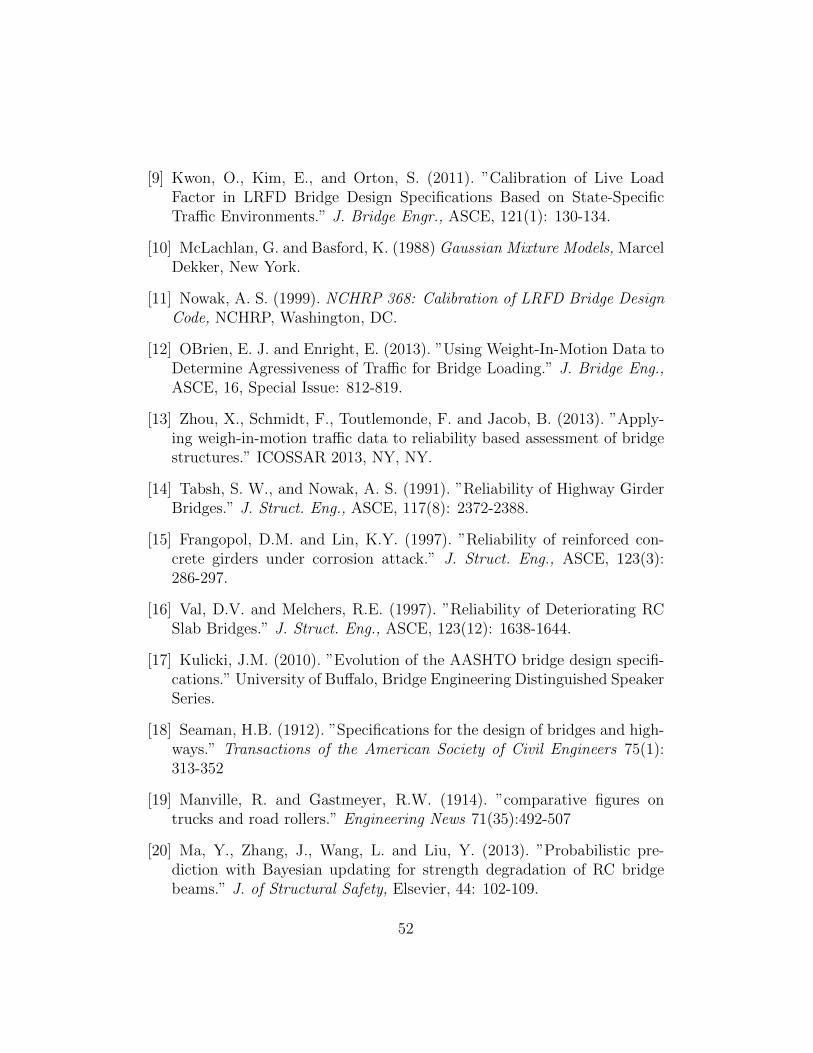
[9] Kwon, O., Kim, E., and Orton, S. (2011). ”Calibration of Live LoadFactor in LRFD Bridge Design Specifications Based on State-SpecificTraffic Environments.” J. Bridge Engr., ASCE, 121(1): 130-134.

[10] McLachlan, G. and Basford, K. (1988) Gaussian Mixture Models, MarcelDekker, New York.

[11] Nowak, A. S. (1999). NCHRP 368: Calibration of LRFD Bridge DesignCode, NCHRP, Washington, DC.

[12] OBrien, E. J. and Enright, E. (2013). ”Using Weight-In-Motion Data toDetermine Agressiveness of Traffic for Bridge Loading.” J. Bridge Eng.,ASCE, 16, Special Issue: 812-819.

[13] Zhou, X., Schmidt, F., Toutlemonde, F. and Jacob, B. (2013). ”Apply-ing weigh-in-motion traffic data to reliability based assessment of bridgestructures.” ICOSSAR 2013, NY, NY.

[14] Tabsh, S. W., and Nowak, A. S. (1991). ”Reliability of Highway GirderBridges.” J. Struct. Eng., ASCE, 117(8): 2372-2388.

[15] Frangopol, D.M. and Lin, K.Y. (1997). ”Reliability of reinforced con-crete girders under corrosion attack.” J. Struct. Eng., ASCE, 123(3):286-297.

[16] Val, D.V. and Melchers, R.E. (1997). ”Reliability of Deteriorating RCSlab Bridges.” J. Struct. Eng., ASCE, 123(12): 1638-1644.

[17] Kulicki, J.M. (2010). ”Evolution of the AASHTO bridge design specifi-cations.” University of Buffalo, Bridge Engineering Distinguished SpeakerSeries.

[18] Seaman, H.B. (1912). ”Specifications for the design of bridges and high-ways.” Transactions of the American Society of Civil Engineers 75(1):313-352

[19] Manville, R. and Gastmeyer, R.W. (1914). ”comparative figures ontrucks and road rollers.” Engineering News 71(35):492-507

[20] Ma, Y., Zhang, J., Wang, L. and Liu, Y. (2013). ”Probabilistic pre-diction with Bayesian updating for strength degradation of RC bridgebeams.” J. of Structural Safety, Elsevier, 44: 102-109.

52

[21] Melchers, R.E. (1999). Structural Reliability Analysis and Prediction.John Wiley and Sons, Ltd. West Sussex, England

[22] van de Lindt, J.W., Fu, G., Zouh, Y., and Pablo, R. (2005). ”Localityof Truck Loads and Adequacy of Bridge Design Load.” J. Bridge Engr.,,ASCE, 10(5): 622-629.

[23] van de Lindt, J.W. and S., Pei. (2006). ”Buckling Reliability of Dete-riorating Steel Beam Ends.” Electronic Journal of Struct. Engineering,2006(6): 1-7.

[24] http://www.census.gov/census2000/states/vt.html

[25] Stewart, M.G. and Rosowki, D.V. (1998) ”Time-dependent reliabilityof deteriorating reinforced concrete bridge decks.” J. Structural Safety,Elsevier, (20):91-109

53

Chapter 4

Bayesian Model AveragingMethods for Identifying LiveLoad Stress Demand ExtremeValue Distributions in Bridges

This paper proposes the use of the Bayesian Model Averagingto identify the optimal model of the extreme values of internalforces in bridge decks from weigh-in-motion (WIM) data. Theidentified models are used for reliability analysis of bridge decks.The weigh-in-motion data was collected by the Vermont Agencyof Transportation during a period of 12 years. The paper presentsa comparision between the demands induced by the WIM dataand the AASHTO HL-93 live load model.

4.1 Introduction

The study of the occurrence of low probability/high consequence events isa crucial aspect of developing a probabilistic design code. The AASHTOLRFD Bridge Design Specifications were generated through such studies.The goal of this code is to provide load and resistance factors consistentwith a reliability index (β) of 3.5 for a service life of 75 years [7]. In orderto do this, the occurrence of extreme loading events needs to be carefullyconsidered. Since 75 years of continuous data are not available, methods for

54

extrapolating smaller periods of data to the 75 year design life are necessary.This extrapolation often involves making assumptions about the behaviorof traffic that can influence the results [3, 4]. Despite this, it is generallyagreed upon that extreme value theory provides an adaquate method forthis extrapolation.

Many researchers have been able to use extreme value analysis to calcu-lated lifetime characteristic load effects for bridge spans [2, 10]. Others [9]modeled truck loads by using the most extreme trucks by weight. Althoughthis may not be completely consistent with extreme value theory, the anal-ysis was able to show that using only extreme values by weight to evaluatetruck load models is possible. A strong correlation between gross vehicleweight (GVW) and and a vehicle producing a maximum stress demand hasbeen observed [6]. However, axle layout has a more significant effect onthis outcome [4]. This is especially true in short and medium span bridges(L ≤ 50m) where the length of a truck might exceed the length of the span.These types of bridges are important because they constitute the largest partof the bridge population. This study focuses on bending moment demand inshort and medium span bridges.

The data for this study comes from 4 Weigh-In Motion (WIM) stations inthe state of Vermont taken over a twelve year period (2000-2011). These sta-tions collect truck axle weights and spacing data, among other things. Fromthis data the maximum bending moment each truck produces in a simplespan can be calculated using structural analysis algorithms. The data werealso time stamped so the moments can be sorted by day of ocurrence. How-ever, no data on speed or headway between vehicles was recorded, so multiplepresence can not be assessed. The maximum bending moment produced by avehicle in each day was attained because it was of interest to develop a prob-ability model that describes the occurrence of the largest (extreme) bendingmoments. This paper describes the various probability models that weretested, as well as the methods used to test their adaquacy to represent thedata. The best fitting model is then used to perform reliability calculationsfor sample bridge superstructures of varying lengths.

The estimated probability of failure is computed using resistance modelsdeveloped by others [7, 8]. The estimated probability of failure can be com-pared with the target value from AASHTO. A reliability index (β) of 3.5 for75 years corresponds to a probability of failure of 0.000233. Since there isonly 12 years of data available, and less for some stations, we must postulatea probabilistic model for the yearly probability that is consistent with the

55

desired probability for a 75 year service life. To calculate the desired yearlyprobability a binomial model is postulated. If one assumes that the processis stationary and the probability of failure is constant every year, one findsthat a Bernoulli process would result in a probability of at least one failuregiven by

P [Z < 0] = 1− (1− p)75 (4.1)

where p is the yearly probability of failure. Setting P [Z < 0] = 0.000233one can solve the previous equation and obtain the corresponding yearlyprobability of p = 3.1 × 10−6. This can then be used to find the 12 (or 10)year failure probability by

P [Z < 0] = 1− (1− p)12 (4.2)

resulting in a 12 year probability of p12 = 3.72×10−5 and a 10 year probabilityof p10 = 3.1× 10−5. These probabilities will be compared to the estimates ofthe probability of failure computed using WIM data.

4.2 The Data

The data was extracted by taking the maximum value from a certain eachday over the data set. This is different from what has been done in thepast [6, 9]. Commonly, the heaviest or largest 5% of the data is taken andused for the data. This is not consistent with extreme value theory, andthe potential issues with this are not discussed in this paper, for more detailsee [5]. A histogram of the data is shown in fig. 4.1. The difference betweenthe distribution of the data in fig. 4.1 and figs. 4.2 and 4.3 is drastic. Fig. 4.2shows the histogram of the largest 5% of moments with the AASHTO valuedenoted by a red line, along with the percent of cases over AASHTO. Fig. 4.3shows the bending moments that resulted from the heaviest 5 % of trucks.It is clear that selecting data in either of these manners will lead to verydifferent conclusions about design values of bending moments than selectingthe daily extreme value. This can be seen in two key ways. The first is theextreme difference in the fraction of cases that exceeded the AASHTO value,this value is three times greater when using the daily maximum moments.The second is the difference in the shape of the distributions. If one were tofit a distribution to the maximum daily moments it would be a completely

56

different fit from the largest 5% of the moments. In order to be consistentwith extreme value theory the maximum daily moments were used for thisstudy.

4.3 Extreme Value Theory

Extreme value theory states that one of three extreme value distributions,Gumbel, Frechet, or Weibull, will describe the distribution of extreme (max-imum or minimum) values of independent and identically distributed (iid)variates. These distributions are all part of a family called the General-ized Extreme Value (GEV) distribution. Formally, the GEV distributionis a limiting distribution of the extrema of n iid random variables, Xi, asn → ∞. Each Xi was the maximum daily bending moment. Which of thethree distributions best describes the maxima/minima depends on the parentdistribution of the variates. In the case of the bending moments, the par-ent distribution of the daily bending moment is unknown. Therefore othermethods to evauluate the appropriateness of each distribution were used andare discussed later in this paper.

For the Gumbel, the parent distribution of the Xi is in the form offx(x) = e−g(x) with dg

dx> 0. The normal, exponential, and gamma distri-

butions all have this form. An important aspect to consider is that in realityrandom variables are hardly ever independent or identical. According toGumbel this condition does not need to completely satisfied in order to usethis distribution (Gumbel, 1958). This is particularly helpful in the case ofthe bending moment data, since it is virtually impossible to prove that thetruck data is independent or identicaly distributed when examined from adaily persepctive.

For the Frechet, the distribution of the Xi is of the form fx(x) =kAx−(k+1), where x > 0 and A is a constant. Distributions of this familyinclude the Cauchy and Pareto. This distribution is one sided, an importantaspect because the bending moments considered are all the same sign. Theunderlying, or parent, distributions for the type II usually have longer tailsthan those of the type I. The distribution of the maximum bending momentsproduced by every truck has a very long tail, further suggesting this is astrong potential candidate distribution.

For the Weibull the parent distribution is fx(x) = Ak(w − x)k−1, withx ≤ w and A a constant. Examples of these types of distributions are the

57

uniform, triangular, and gamma. This distribution is typically used whenXi is limited in the tail of interest to a maximum value w. Like the typeII, this is also a one sided distribution. Although the Weibull dsitributionis typically used for failure, the flexibility of the distribution to fit a widevariety of data makes it useful for this situation. The thought here is thatif Weibull analysis can provide good failure forecasts with little data, it canalso forecast the occurrence of large stress demands with similar accuracy(Abernathy, 2006).

4.4 Daily Maximum Bending Moments and

Extreme Value Theory

The condition that populations from which the extremes are being sampledare iid needs to be met in order to use extreme value theory. If this doesnot hold then none of the asymptotic distributions will suffice to representthe extremes. This is because the derivation of the asymptotic distributionsis based on the iid asumption. This assumption is such that probability ofthe extremes being less than a certain value is a function of the cumulativedistribution of the population which the extremes came from:

P [X1, X2, ..., Xn ≤ x] = FX(x)n (4.3)

If this does not hold true the stability postulate cannot be applied so theasymptotic distribution of the extremes does not converge to a GEV distri-bution [5]. Therefore examination of the distribution of the daily bendingmoments is necessary.

From fig. 4.4 it is clear that the daily bending moments do not have thesame parent distribution. Although they all appear to be mixture distribu-tions, the weights, means, and standard deviations of the moxture compo-nents appear to be completely different from day to day. Clearly this violatedthe iid assumption necessary to invoke extreme value theory. Therefore wewill consider other distributions, as well as the GEV distributions, as poten-tial proabbility models for the daily maximum bending moments.

58

4.5 Probability Models

The following sections describe the various probability distributions that weretested for their fit to the data. Six probability distributions were tested tofit the data in this study. Since the iid condition necessary to use extremevalue theory was not satisfied 3 additional distributions were tested. Theseother diustributions, the Gaussian, log-normal, and Gamma distributions,were selected based on the shape of the data histogram. These three werethought to have the most potential to fit the data outside of the three GEVdistributions because of their shape. The following sections explain how theparameters for each model were estimated.

4.5.1 Normal Models

Gaussian (normal) and log-normal distributions were considered as potentialmodels because of their shape. In fig. 1 the data appear to have a similarshape to these types of distributions. The mean and variance of the data arethe parameters for the Gaussian and are easily obtained. For the log-normaldistribution the parameters were transformed using the following equations,with m and v representing the mean and variance of the data respectively.Plots of these distributions over the data are shown in fig. 2.

µ = log

(m2

√v +m2

)(4.4)

σ =

√log(1 +

v

m2) (4.5)

4.5.2 GEV Models

As previously stated, all three types of GEV distributions were tested. TheGEV Type I distribution is descibed by the following PDF:

fy(y) = αe−α(y−u)−e−α(y−u) (4.6)

The parameters α and u are estimated from the data using the followingequations (γ is Euler’s constant):

E[y] = µy = u+γ

α(4.7)

59

V ar[y] = σ2y =

π2

6α2(4.8)

The GEV Type II distribution is described by the following PDF:

fy(y) =k

y

(u

k

)ke−(u/y)k (4.9)

The parameter estimation for this distribution is less straightforward.This is because the definition of the moments involves using the gammafunction. The estimation is done using the following equations:

E[y] = µy = uΓ(1− 1/k) (4.10)

V ar[y] = σ2y = u2[Γ(1− 2/k)− Γ2(1− 1/k)] (4.11)

These can be combined to eliminate u and k can be estimated by theguess and test method using the following equation:

µ2y

σ2y

=Γ(1− 2/k)

Γ2(1− 2/k)− 1 (4.12)

The Weibull distribution is described by the following PDF:

fy(y) =β

α

(y

α

)β−1

e−(y/α)β (4.13)

The shape parameter β is estimated iteratively using the following equa-tion:

1

β=

∑Ni=1(yki ln yi − ykN ln yN)∑N

i=1(yki − ykN)− 1

N

N∑i=1

ln yi (4.14)

Once the shape parameter has been obtained the definition of the firstmoment, or expected value, can be used to estimate the scale parameter α.Like the GEV type II, the expected value is defined as:

E[y] = αΓ(1 +1

k) (4.15)

This leads to:

60

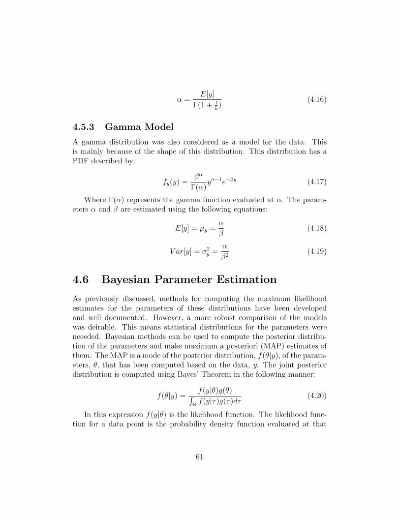
α =E[y]

Γ(1 + 1k)

(4.16)

4.5.3 Gamma Model

A gamma distribution was also considered as a model for the data. Thisis mainly because of the shape of this distribution. This distribution has aPDF described by:

fy(y) =βα

Γ(α)yα−1e−βy (4.17)

Where Γ(α) represents the gamma function evaluated at α. The param-eters α and β are estimated using the following equations:

E[y] = µy =α

β(4.18)

V ar[y] = σ2y =

α

β2(4.19)

4.6 Bayesian Parameter Estimation

As previously discussed, methods for computing the maximum likelihoodestimates for the parameters of these distributions have been developedand well documented. However, a more robust comparison of the modelswas deirable. This means statistical distributions for the parameters wereneeeded. Bayesian methods can be used to compute the posterior distribu-tion of the parameters and make maximum a posteriori (MAP) estimates ofthem. The MAP is a mode of the posterior distribution, f(θ|y), of the param-eters, θ, that has been computed based on the data, y. The joint posteriordistribution is computed using Bayes’ Theorem in the following manner:

f(θ|y) =f(y|θ)g(θ)∫

Θf(y|τ)g(τ)dτ

(4.20)

In this expression f(y|θ) is the likelihood function. The likelihood func-tion for a data point is the probability density function evaluated at that

61

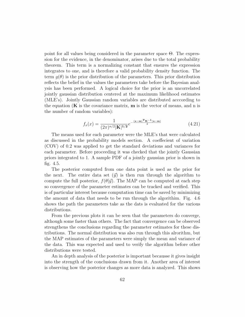
point for all values being considered in the parameter space Θ. The expres-sion for the evidence, in the denominator, arises due to the total probabilitytheorem. This term is a normalizing constant that ensures the expressionintegrates to one, and is therefore a valid probability density function. Theterm g(θ) is the prior distribution of the parameters. This prior distributionreflects the belief in the values the parameters take before the Bayesian anal-ysis has been performed. A logical choice for the prior is an uncorrelatedjointly gaussian distribution centered at the maximum likelihood estimates(MLE’s). Jointly Gaussian random variables are distributed acccording tothe equation (K is the covariance matrix, m is the vector of means, and n isthe number of random variables):

fx(x) =1

(2π)n/2|K|1/2e−

(x−m)TK−1(x−m)2 (4.21)

The means used for each parameter were the MLE’s that were calculatedas discussed in the probability models section. A coeffecient of variation(COV) of 0.2 was applied to get the standard deviations and variances foreach parameter. Before proceeding it was checked that the jointly Gaussianpriors integrated to 1. A sample PDF of a jointly gaussian prior is shown infig. 4.5.

The posterior computed from one data point is used as the prior forthe next. The entire data set (~y) is then run through the algorithm tocompute the full posterior, f(θ|~y). The MAP can be computed at each stepso convergence of the parameter estimates can be tracked and verified. Thisis of particular interest because computation time can be saved by minimizingthe amount of data that needs to be run through the algorithim. Fig. 4.6shows the path the parameters take as the dats is evaluated for the variousdistributions.

From the previous plots it can be seen that the parameters do converge,although some faster than others. The fact that convergence can be observedstrengthens the conclusions regarding the parameter estimates for these dis-tributions. The normal distribution was also run through this alrorithm, butthe MAP estimates of the parameters were simply the mean and variance ofthe data. This was expected and used to verify the algorithm before otherdistributions were tested.

An in depth analysis of the posterior is important becausse it gives insightinto the strength of the conclusions drawn from it. Another area of interestis observing how the posterior changes as more data is analyzed. This shows

62

how the belief goes from a spread out jointly gaussian prior into a muchsharper and more precise estimate of the parameters. Fig. 4.7 shows theevolution of the posterior distribution of the GEV type I parameters as moredata us evaluated. This contour plot was generated every 350 data pointsthroughout the entire data set analysis.

These two figures are important for examing the behavior of the posterior,because this gives us informatuion about the accuracy of the parameter es-timates. The contours are significantly stretched along the α direction. Thismeans that this parameter converges slower, which can also be seen in theprevious figure that traces the MAP estimate of α. This behavior remainsconstant throughout the evolution of the posterior. Although the peak be-comes much sharper throughout this process, this means that there is moreuncertainty on the true value of α than u. The higher uncertainty can alsobe seen in the ranges of the credible intervals. A credible interval representsthe interval that the true value of the parameter has a certain probability offalling within. The 95% credible interval for α is 7.0171×10−4−7.4735×10−4

and 5.6798× 103 − 5.8345× 103 for u.Fig. 4.8 shows a similar behavior for the GEV Type II posterior. Here,

the difference in uncertainty is less pronounced, but the uncertainty on thetrue value of u is still significantly less than than than of k. The credibleitnerval for u is 5.4876 × 103 − 5.6640 × 103 and 3.5441 − 3.7352 for k. Itonly takes about 500 data points for u to converge within 5% of its MAPvalue, while k appears to be trending thowards a MAP value, but does notappear to have completely converged for the total amount of data available.This was the only instance where a parameter appeared to not completelyconverge. In fig. 4.6 all parameters for all other distributions appear to haveleveled off in the neighborhood of the MAP estimates.

The difference in uncertainty on the Weibull parameters is noticably less,as shown in fig. 4.9. However, there is still more uncertainty on the true valueof β than on α. The 95 % credible interval for α is 6.96341×103−7.1418×103

and 4.5790−4.8564 for β. This was expected since fig. 4.6 shows α convergingfaster than β. The value of α gets to and stays within 5% of the MAP roughly550 points before the value of β does.

The uncertainty on the gamma parameters was shared evenly between theparameters α and β. This can be seen by the almost one-to-one line formedby the posterior in fig. 4.10. When looking at the convergence of theseparameters this shared uncertainty makes sense. Both parameters appear tohave coverged at an alomst identical rate, suggesting that the uncertainty

63

on them is similar. The MAP estimates were only slightly different than theMLE estimates. The MAP estimate for α was 20.69, while the MLE was20.92. The 95% credible interval was 18.0931−20.1947. For β the MAP andMLE were 7.24x10−4 and 7.32x10−4 respectively. The 95 % credible intervalwas 2.7820× 10−3 − 3.1109× 10−3.

The uncertainty on the log-normal and Gaussian parameters was virtuallynonexistent, the credible intervals were roughly ±1% of the MLE’s. Thismeans that the posterior modes were very sharp and decayed quickly movingaway from the MLE’s.

4.7 Evaluation of Probability Models

Two tools were used to evaluate the adaquacy of the possible probabilitymodels. These are the Chi-Square test and Bayesian model comparison, bothof which are discussed in this section. The chi-square test is a frequently usedfrequentist method of testing the fit of a probability model to data. Bayesianmodel comparison is a newer method of model evaluation that is ideal forapplications with large amounts of data, such as this.

4.7.1 Chi-Square test

The chi-square test is commonly used to determine the goodness of fit ofa distribution to a data set. The basic idea is to determine the chance ofobserving a result as extreme as the data if it does come from the postulateddistribution. If it turns out that this chance, called the observed significancelevel, is greater than a desirted and pre-dtermined significance level (α, typi-cally 0.01 or 0.05) then the data cannot be described by the proposed model.The steps to carry out the test are as follows:

1. Divide the sample space SX into K disjoint intervals (bins).

2. Calculate the probability bk than an outcome falls within the kth in-terval based on the assumption that X has the postulated CDF. Setmk = nbk where mk is the expected number of outcomes that fall inthe kth interval if the experiment is repeated n times.

3. Calculate the chi-square statistic as the weighted difference between theobserved number of outcomes in each interval (Nk) and the expectednumber (mk) using the following equation:

64

D2 =K∑k=1

(Nk −mk)2

mk

4. D2 is then compared to a threshold value (talpha). If D2 > tα the pro-posed distribution is an acceptable model for the data. This thresholdvalue is determined from a chi-square PDF with K − 1 degrees of free-dom and follows the following equation:

P [X ≥ tα] = α

This test was performed on each of the proposed probability models. Eachdistribution is shown over the data in fig. 4.11. The Chi-Square statistic foreach distribution is also shown on these plots. The threshold value for a 0.05significance level using 30 bins is 42.56. This means that the test showedthat none of the models was a particularly good fit for the data. Thereforeanother means for evaluating the models was needed.

4.7.2 Bayesian Model Averaging

Since the chi-square test was incinclusive, Bayesian model averaging providedan alternative and more conclusive way of comparing the models for the data.This method for model comparisson uses Bayesian methods to compute thebelief that each model is a propper fit for the data. To start, first considerwhat is occurring onthe individual model level. Bayes’ theorem is used tocalculate the probability of observing the data if each model were correct(P [y|Mi]). For a given model and set of parameters θ, the probability densityfunction of the parameters given the data is found using Bayes’ Theorem (eq.17). The evidence is proportional to the predictive strength of the model.This leads to:

P [y|Mi] =

∫Θ

f(y|θ)f(θ)dθ (4.22)

The models can be compared using the probability of observing the datagiven each model. This requires a probability mass function that definesthe prior belief in each model (P [Mi]). Bayes theorem is used again hereto develop an expression for the probability of the model being the best fitgiven the data (P [Mi|y]):

65

Table 4.1: Results of Model Averaging

Distribution ProbabilityLog-Normal 0.0

Gaussian 0.3495GEV Type-I 0.0

Gamma 0.6505GEV Type-II 0.0

Weibull 0.0

f(Mi|y) =P [y|Mi]P [Mi]

m∑j=1

P [y|Mj]P [Mj](4.23)

Again, to compare multiple models, the jointly gaussian distribution cen-tered at the parameter MEL’s were used for the parameter priors. Thelikelihood for a data point was simply the probability model evaluated atthat point for all possible values of the parameter. Numerical integrationwas used to compute the evidence.

The prior for each model was considered to be 1/6 since it was not clearwhich model would be the best fit from the previous analysis performed. Forthe model comparison, the evidence calculated for each model at a givenpoint was used as the likelihood for that model. The total evidence for ateach point was then computed as the sum of the individual likelihoods timesthe corresponding model priors, as shown in the denominator of equation 19.The posterior probability was therefore the likelihood of the model times theprior for the model divided by the evidence. This process was repeated forevery point in the data set with the posterior being used as the new prior.The belief in each model is then updated every time a new data point isconsidered. Afrter running through the entie data set the model that bestfits will have the highest posterior value. Different values for the COV wereused after the initial analysis was performed. This was to examine the effectthat the COV had on the results. It was determined that a 100% increase inthe COV resulted in less than a 1% change in the results.

The results of the Bayesian model averaging are shown in table 1. TheGaussian and Gamma distributions are overwhelmingly favored: the belief

66

in all other models rounds to zero from over 10 decimal places. The data wasrun sequentially starting with the maximum bending moment from the firstday of data. The belief in each probability model that was found using Bayes’rule can be used as weights to form a mixture distribution. The evolutionof these weights, or mixing coeffecients, as the data was run are shown infig. 4.12. It can be seen that the belief that the Log-Normal, GEV Type-I,GEV Type-II, and Weibull models diminishes quickly, while the belief in theGaussian and Gamma models fluctuates throughout the process.

These beliefs can be thought of as weights for a mixture distribution. Inthis case the mixture is of Gaussian and Gamma distributions. The Log-Normal and GEV Type-I distributions are excluded from this because oftheir large chi square statistics and virtually zero belief as found using Bayes’Theorem. Since it is not evident that the belief in the Gamma and Gaussiancoverged, different weights were tested ranging between 0.3-0.7 for each dis-tribution. The mixture distribution is shown over the data in fig. 4.13 alongwith the Chi-Square statisitc for this distribution. This mixture distributionis a better fit visually and mathematically than to the other distributions(shown in fig. B.3), as seen through the Chi-Square statistic. The criticalvalue for the 0.05 significance level is 42.6, so the distribution passes the test.

4.8 Results

The purpose of this project was to combine the credible intervals on theparameters and model comparisson results to model the live load stress de-mands. To do this, the distributions, with each combination of parameterestimates, were mixed according to the model comparrison results. Using thelower bound of α with corresponding value of β found using equation 15 gavevalues of .3860 of cases over AASHTO, while using the upper bound of α andcorresponding value of β gave a value of .3809 of cases over AASHTO. Re-peating the same procedure for the upper and lower values of β led to resultswithin 2% of the values for when the upper and lower bounds of α were used.This showed that the uncertainty on the parameter values results in minimaluncertainty on the probability of exceeding AASHTO. These distributionscan then be used to perform reliability calculations on bridge girders.

In order to complete a full live load reliability analysis for the superstruc-ture, the dead load and girder resistances needed to be calculated. This wasdone by using AASHTO to design bridges that were as close to the minimum

67

Table 4.2: Results of Reliability Analysis

Estimated Probability of FailureStation L=10m L=20mR100 4.86× 10−8 1.89× 10−6

X249 7.45× 10−8 5.83× 10−8

G005 1.30× 10−7 1.39× 10−5

R001 1.84× 10−7 2.11× 10−6

Table 4.3: Results of Reliability Analysis Using GEV Distribution for theLive Load

Estimated Probability of FailureStation L=10m L=20mR100 1.75× 10−5 6.95× 10−5

X249 1.55× 10−6 3.66× 10−5

G005 1.42× 10−5 6.44× 10−5

R001 4.69× 10−6 2.21× 10−5

requirements for strength as possible. From the superstructure design, thedead load and resistances could be calculated. The dead load and resistancewere then assigned distributions based on available literature [7]. SAP2000was used to model the bridge decks to determine the maximum amount oflive load that each girder would need to support.

Table 2 shows the estimated probability of failure for the 4 WIM stationsconsidered for both 10 and 20 meter length spans. The probability modelused for the live load was the mixture determined using Bayesian ModelAveraging. The values here are all at least one order of magnitude smallerthan the 10 and 12 year target values given in the introduction. Table 3shows the estimated probability of failure using a GEV type I distributionfor the live load. In all cases there is a noticable difference in the estimatedprobability of failure, with the estimate using a GEV distribution for the liveload much larger. In all but one case this difference is greater than one orderof magnitude.

68

This large difference in estimated probability of failure can be attributedto the shape of the tail of the GEV type I distribution. The GEV typeI with MAP parameters and the best fitting distribution are shown in fig.4.14. The tail of the GEV distribution is noticably heavier than the tail ofthe best fit. A convolution is used to add the dsitribution of the live loadeffects to the distribution of the dead load effects. A cross corelation is thenused to subtract the distribution of the load effects from the distribution ofthe resistance. These two processes compound the effect of the heavier tail,as can be seen in the difference in estimated probability of failure.

4.9 Conclusion

The results of this study show that using extreme value theory to model liveload effects in bridge spans can lead to over estimating the probability offailure. Other distributions, or mixtures of other distributions, have beenshown to better fit the extreme values of the live load effects. The reason forthe difference in probability of failure is that these other distributions havelighter tails than the GEV dsitributions. Furthermore, it has been shownthat the parent distributions that the extreme load effects come from are notidentical. This violates one of the necessary conditions to use extreme valuetheory.

Bayes’ Theorem has been shown to be a powerful method for determiningthe optimal probability model for these load effects have been developed. Wehave shown that this method result in better fitting probability models thansimply using extreme value theory. Furthermore, the optimal parametersfor these probability models vary from the maximum likelihood estimates.Bayesian methods also provide suitable methods for determining the param-eters.

4.10 Figures

69

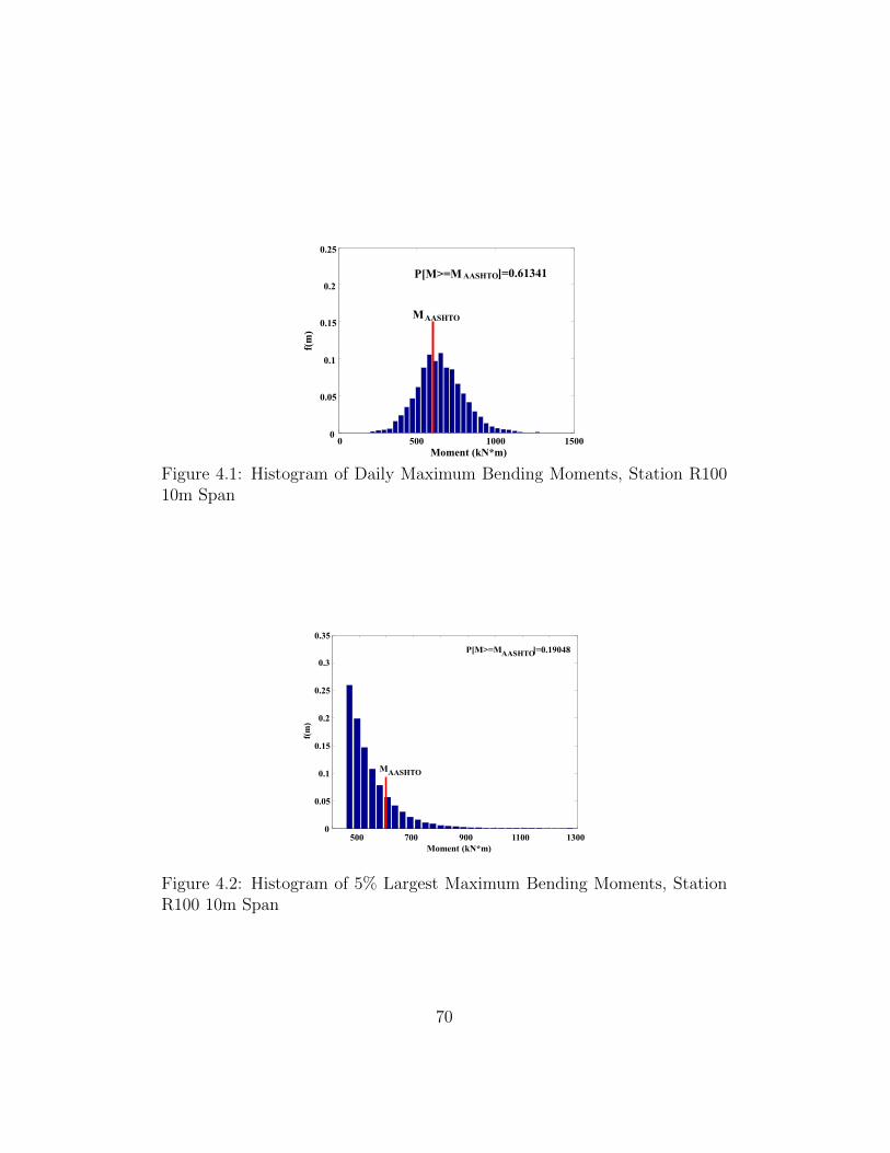
0 500 1000 1500 0

0.05

0.1

0.15

0.2

0.25

Moment (kN*m)

f(m

)

P[M>=M AASHTO ]=0.61341

M AASHTO

Figure 4.1: Histogram of Daily Maximum Bending Moments, Station R10010m Span

500 700 900 1100 1300 0

0.05

0.1

0.15

0.2

0.25

0.3

0.35

Moment (kN*m)

f(m

)

P[M>=M AASHTO ]=0.19048

M AASHTO

Figure 4.2: Histogram of 5% Largest Maximum Bending Moments, StationR100 10m Span

70

400 600 800 1000 1200 0

0.04

0.08

0.12

0.16

0.2

Moment (kN*m)

f(m)

P[M>=M AASHTO ]=0.16313

M AASHTO

Figure 4.3: Histogram of Maximum Bending Moments from 5% HeaviestVehicles, Station R100 10m Span

100 200 300 400 500 600 700 0

1

2

3

4

5

6

7

8

200 400 600 800 1000 0

1

2

3

4

5

6

100 200 300 400 500 600 700 0

1

2

3

100 200 300 400 500 600 700 0

1

2

3

4

5

6 x 10 -4

x 10 -4 x 10 -4

x 10 -4

Figure 4.4: Histograms of Maximum Bending Moments for Randomly Se-lected Days from Station R001 in 2006

71

100 200 300 400 500 600 700 800 900 1000

100

200

300

400

500

600

700

800

900

1000

0

X2

X1

Figure 4.5: Independent Jointly Gaussian PDF

72

0 500 1000 1500 2000 2500 3000 3500 2

3

x 10 -4 GEV Type I Parameters

a

0 500 1000 1500 2000 2500 3000 3500 0.5

1

1.5

2 x 10 4

u

Number of Points 0 500 1000 1500 2000 2500 3000 3500

2.5

3

3.5

4 GEV Type II Parameters

k 0 500 1000 1500 2000 2500 3000 3500

0.5

1

1.5

2 x 10 4

u

Number of Points

0 500 1000 1500 2000 2500 3000 3500 1.2

1.4

1.6

1.8

2 x 10 4 Weibull Parameters

a

0 500 1000 1500 2000 2500 3000 3500 3

4

5

6

b

Number of Points

0 500 1000 1500 2000 2500 3000 3500 10

15

20

25 Gamma Parameters

a

0 500 1000 1500 2000 2500 3000 3500 0.5

1

1.5 x 10 -3

b

Number of Points

0 500 1000 1500 2000 2500 3000 3500 9.2

9.4

9.6

9.8 Log-Normal Parameters

m

0 500 1000 1500 2000 2500 3000 3500

0.2

0.25

0.3

0.35

s 2

Number of Points

Figure 4.6: Behavior of Parameters as Data is Evaluated

73

u

1.35 1.4 1.45 1.5 1.55 1.6

x 10-4

2.4

2.5

2.6

2.7

2.8x 10

4

u

1.6 1.65 1.7 1.75 1.8 1.85 1.9

x 10-4

2.3

2.4

2.5

2.6

2.7

x 104

u

1.7 1.75 1.8 1.85 1.9 1.95 2

x 10-4

2.3

2.4

2.5

2.6

2.7

x 104

u

1.65 1.7 1.75 1.8 1.85 1.9 1.95

x 10-4

2.3

2.4

2.5

2.6

2.7x 10

4

u

1.6 1.65 1.7 1.75 1.8 1.85 1.9

x 10-4

2.3

2.4

2.5

2.6

2.7

x 104

u

1.55 1.6 1.65 1.7 1.75 1.8 1.85

x 10-4

2.3

2.4

2.5

2.6

2.7

x 104

u

1.55 1.6 1.65 1.7 1.75 1.8 1.85

x 10-4

2.3

2.4

2.5

2.6

2.7

x 104

u

1.55 1.6 1.65 1.7 1.75 1.8 1.85

x 10-4

2.3

2.4

2.5

2.6

2.7

2.8x 10

4

u

1.55 1.6 1.65 1.7 1.75 1.8 1.85

x 10-4

2.4

2.5

2.6

2.7

2.8x 10

4

350 Points 700 Points 1050 Points

2100 Points 1750 Points 1400 Points

2450 Points 2800 Points 3160 Points

Figure 4.7: Evolution of GEV Type I Posterior

74

k

u

2.8 2.9 3 3.1 3.2 3.3 3.4

2.3

2.4

2.5

2.6

2.7x 10

4

k

u

3.3 3.4 3.5 3.6 3.7 3.8 3.9

2.2

2.3

2.4

2.5

2.6

x 104

k

u

3.6 3.8 4 4.2

2.2

2.3

2.4

2.5

2.6

x 104

k

u

3.6 3.8 4 4.2

2.2

2.3

2.4

2.5

2.6

x 104

k

u

3.6 3.8 4 4.22.2

2.3

2.4

2.5

2.6

x 104

k

u

3.2 3.3 3.4 3.5 3.6 3.7 3.82.2

2.3

2.4

2.5

2.6

x 104

k

u

3.2 3.3 3.4 3.5 3.6 3.7 3.8

2.3

2.4

2.5

2.6

x 104

k

u

3.2 3.3 3.4 3.5 3.6 3.7 3.8

2.3

2.4

2.5

2.6

2.7

x 104

k

u

3.3 3.4 3.5 3.6 3.7 3.8 3.9

2.3

2.4

2.5

2.6

2.7

x 104

350 Points 700 Points 1050 Points

2100 Points 1750 Points 1400 Points

2450 Points 2800 Points 3160 Points

Figure 4.8: Evolution of GEV Type II Posterior

75

350 Points 700 Points 1050 Points

2100 Points 1750 Points 1400 Points

2450 Points 2800 Points 3160 Points

2.9 3 3.1 3.2 3.3 3.4 3.5

x 104

4

4.2

4.4

4.6

4.8

2.8 2.9 3 3.1 3.2 3.3

x 104

4.2

4.4

4.6

4.8

5

2.7 2.8 2.9 3 3.1 3.2

x 104

4.4

4.6

4.8

5

5.2

2.7 2.8 2.9 3 3.1 3.2

x 104

4.2

4.4

4.6

4.8

5

2.8 2.9 3 3.1 3.2 3.3

x 104

4.2

4.4

4.6

4.8

2.8 2.9 3 3.1 3.2 3.3

x 104

4.2

4.4

4.6

4.8

2.8 2.9 3 3.1 3.2 3.3

x 104

4.2

4.4

4.6

4.8

5

2.8 2.9 3 3.1 3.2 3.3 3.4

x 104

4.4

4.6

4.8

5

2.8 2.9 3 3.1 3.2 3.3 3.4

x 104

4.4

4.6

4.8

5

Figure 4.9: Evolution of Weibill Posterior

76

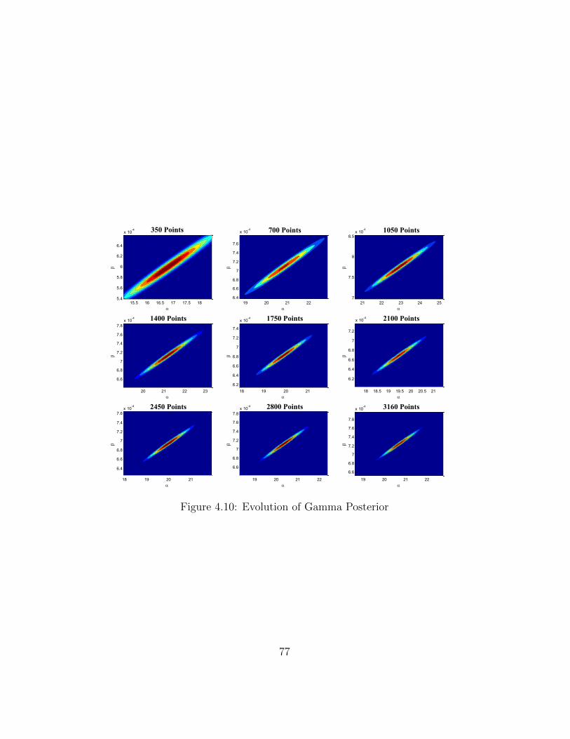
350 Points 700 Points 1050 Points

2100 Points 1750 Points 1400 Points

2450 Points 2800 Points 3160 Points

15.5 16 16.5 17 17.5 185.4

5.6

5.8

6

6.2

6.4

x 10-4

19 20 21 226.4

6.6

6.8

7

7.2

7.4

7.6

x 10-4

21 22 23 24 257

7.5

8

8.5x 10

-4

20 21 22 23

6.6

6.8

7

7.2

7.4

7.6

7.8x 10

-4

18 19 20 216.2

6.4

6.6

6.8

7

7.2

7.4

x 10-4

18 18.5 19 19.5 20 20.5 21

6.2

6.4

6.6

6.8

7

7.2

x 10-4

18 19 20 21

6.4

6.6

6.8

7

7.2

7.4

7.6x 10

-4

19 20 21 22

6.6

6.8

7

7.2

7.4

7.6

7.8x 10

-4

19 20 21 22

6.6

6.8

7

7.2

7.4

7.6

7.8

x 10-4

Figure 4.10: Evolution of Gamma Posterior

77

0 2 4 6 8 10 12 14 0

1

2

x 10 -4 Log-Normal Fit Over Data

Moment(kN*m)

f(m

)

c 2 =497.2516

x 10 3

0

1

2

x 10 -4 Gaussian Fit Over Data

f(m

)

c 2 =98.7393

0 2 4 6 8 10 12 14 Moment(kN*m) x 10 3

0

1

2

x 10 -4 Gamma Fit Over Data

c 2 =101.2524

f(m)

0 2 4 6 8 10 12 14 Moment(kN*m) x 10 3

0

1

2

x 10 -4 GEV Type-I Fit Over Data

c 2 =874.1475

f(m

)

0 2 4 6 8 10 12 14 Moment(kN*m) x 10 3

0

1

2

x 10 -4 Weibull Fit Over Data

c 2 =1318.6041

0 2 4 6 8 10 12 14 Moment(kN*m) x 10 3

GEV Type II Fit Over Data

0

1

2

x 10 -4

c 2 =53235471.5769

0 2 4 6 8 10 12 14 Moment(kN*m) x 10 3

f(m)

Figure 4.11: Probability models plotted over the data with their respectiveChi-Square statistic

78

0 500 1000 1500 2000 2500 3000 3500 0

0.1

0.2

0.3

0.4

0.5

0.6

0.7

0.8

0.9

1

Number of Points

Bel

ief i

n M

odel

GEV Type-I GEV Type-II Weibull Gamma Log-Normal Gaussian

Figure 4.12: Evolution of Mixing Coeffecients as Data is Run

0 200 400 600 800 1000 1200 1400 0

1

2

x 10 -4

c 2 =32.3036

Moment (kN*m)

f(m

)

D=42.5600

Figure 4.13: Gaussian/Gamma Mixture Fitted Over Data χ2 Statistic

79

0 100 200 300 400 500 600 700 800 900 1000 0

0.5

1

1.5

2

2.5

3

3.5

4

4.5 x 10 -4

Bending Moment (kN*m)

P[M

=m]

GEV Type I Best Fit

Figure 4.14: Comparison of GEV to Best fitting Distribution

80

Bibliography

[1] Abernethy, RB. ”Ch. 1: An Overview of Weibull Analysis.” The NewWeibull Handbook, (5th), North Palm Beach, FL, 2006.

[2] Bailey, S. and Bez, R. (1999) ”Site Specific Probability Distribution ofExtreme Traffic Action Effecs.” J. Probabilistic Engineering Mechanics,Elsevier, 14, 19-26.

[3] Caprani, C., OBrien, E. J., and McLachlan, G. (2007). ”Characteris-tic Traffic Load Effects from a Mixture of Loading Events on Short toMedium Span Bridges.” J. Struct. Safety, Elsevier, 30, 394-404.

[4] Enright, B. and O’Brien, E.J. (2012) ”Monte Carlo Simulation of Ex-treme Traffic Loading on Short and Medium Span Bridges.” Structureand Infrastructure Engineering, Taylor and Francis, 9(12), 1267-1282.

[5] Gumbel, E.J. (1958) Statistics of Extremes, Columbia University Press,New York.

[6] Kwon, O., Kim, E., and Orton, S. (2012). ”Calibration of Live-Load Fac-tor in LRFD Bridge Design Specifications Based on State-Specific TrafficEnvironments.” J. Bridge Eng., ASCE, 16, SPECIAL ISSUE: AASHTO-LRFD Bridge Design and Guide Specifications: Recent, Ongoing, andFuture Refinements, 812819.

[7] Nowak, A. S. (1999). NCHRP 368: Calibration of LRFD Bridge DesignCode, NCHRP, Washington, DC.

[8] Tabsh, S. W., and Nowak, A. S. (1991). ”Reliability of Highway GirderBridges.” J. Struct. Eng., ASCE, 117(8), 2372-2388.

81

[9] Zhao, J. and Tabatabai, H (2012). ”Evaluation of a Permit Vehicle ModelUsing Weight-In-Motion Truck Records.” J. Bridge Eng., ASCE, 17(2),389-392.

[10] Zhou, X., Schmidt, F., Toutlemonde, F., and Jacob, B. ”Apply-ing Weight-In-Motion Data to Reliability Based Assessment of BridgeStructures.” ICOSSAR2013, 11th International Conference on StructuralSafety & Reliability, France.

82

Bibliography

[1] Henry Seaman. Specifications for the design of bridges and highways.Transactions of the American Society of Civil Engineers, 1912.

[2] L.R. Manville and R.W. Gastmeyer. Motor trucks: Loads on highwaybridges. Engineering News, 1914.

[3] A.S. Nowak. Nchrp report 368: Calibration of lrfd bridge design code.Technical report, NCHRP, 1999.

[4] O’Brien E.J. Caprani, C. and G. McLachlan. Characteristic traffic loadeffects from a mixture of loading events on short to medium span bridges.J. Structural Safety, Elsevier, 2007.

[5] Battacharya B. Guzda, M and D. Mertz. Probabilistic characterizationof live load using visual counts and in-service strain monitoring. J.Bridge Engineering, ASCE, 2007.

[6] M. Kozikowski. WIM Based Live Load Model for Bridge Reliability. PhDthesis, University of Nebraska, 2009.

[7] Kim E. Kwon, O. and S. Orton. Calibration of live load factor in lrfdbridge design specifications based on state-specific trafic environments.J. Bridge Engineering, ASCE, 2011.

[8] E.J. O’Brien and B. Enright. Using weight-in-motion data to determineagressiveness of traffic for bridge loading. J. Bridge Engineering, ASCE,2013.

[9] S.W. Tabsh and A.S. Nowak. Reliability of highway girder bridges. J.Struct. Engineering, ASCE, 1991.

83

[10] Fu G Zouh Y. van de Lindt, J.W. and R. Pablo. Locality of truck loadsand adequacy of bridge design load. J. Bridge Engineering, ASCE, 2005.

[11] J.W. van de Lindt and S. Pei. Buckling reliability of deteriorating steelbeam ends. Electronic Journal of Structural Engineering, 2006.

[12] J. Zhao and H. Tabatabai. Evaluation of a permit vehicle model usingweight-in-motion truck records. J. Bridge Engineering, ASCE, 2012.

[13] Schmidt F. Toutlemonde F. Zhou, X. and B. Jacob. Applying weight-in-motion traffic data to reliability based assessment of bridge structures.In ICOSSAR2013, 11th International Conference on Structural Safetyand Reliability.

[14] S.F. Bailey and B. Rolf. Site specific probability distribution of extremetraffic action effects. J. Probabilistic Engineering Mechanics, Elsevier,1999.

[15] B. Enright and E.J. O’Brien. Monte carlo simulation of extreme trafficloading on short and medium span bridges. J. Structure and Infrastruc-ture Engineering, Taylor & Francis, 2013.

[16] American Association of State Highway and Transportation Officials,Washington, D.C. AASHTO LRFD Bridge Design Specifications, 2010.

[17] R.C. Hibbeler. Structural analysis. Pearson Prentice Hall, Upper SaddleRiver, NJ, 7 edition, 2009.

[18] G. McLachlan and K. Basford. Mixture Models: Inference and Applica-tionsto Clustering. Marcel Dekkerl, New York, 1989.

[19] E.J. Gumbel. Statistics of Extremes. Columbia University Press, NewYork, 1958.

84

Appendix A: Axle Statisticsby Station

This section displays the axle statistics for vehicles categorized by WIM sta-tion. The percentage of vehicles with a given number of axles is shown bystation in table A.1. The mean axle weights and spacing, as well as the co-variance matrix are also presented for the 2-7 axle vehicle groups by station.The covariance matrix contains the variance on the diagnals and is symetric.The axle statistics matricies were formed by taking the covariance of the dataorganized in vectors with the following format:

[P1...Pn S1...Sn−1

]

Table A.1: Fraction of Vehicles by Axle Count by Station

Number of Axles Station R100 Station X249 Station G005 Station R0012 0.4469 0.5319 0.6705 0.24183 0.0736 0.0808 0.0894 .05684 0.0577 0.0752 0.0728 .07825 0.2937 0.2901 0.1523 0.57736 0.1277 0.0216 0.0147 50.04527 0.0004 0.0005 0.0003 0.0007∑= 1.0000 1.0000 1.0000 1.0000

85

Table A.2: 2 Axle Vehicle Means for Station R100

µp1 µp2 µs123.77 29.10 43.12

Covariance Matrix for 2 Axle Vehicles178.7 255.9 87.63255.8 542.1 174.587.6 174.5 154.8

Table A.3: 3 Axle Vehicle Means for Station R100

µp1 µp2 µp3 µs1 µs251.75 52.22 45.79 52.88 19.61

Covariance Matrix for 3 Axle Vehicles313.9 289.3 290.8 45.0 −78.6289.3 770.8 602.2 68.4 −2.9290.8 602.2 684.8 6.2 −53.145.0 68.4 6.2 134.4 87.2−78.6 −2.9 −53.1−87.2 340.3

Table A.4: 4 Axle Vehicle Means for Station R100

µp1 µp2 µ(p3) µp4 µs1 µs2 µs341.57 47.38 37.13 34.33 41.04 57.63 23.22

Covariance Matrix for 4 Axle Vehicles

376.3 256.7 449.5 395.9 35.1 −203.5 30.6256.7 611.4 385.0 276.9 30.1 179.7 −55.2449.5 385.0 874.0 724.8 36.0 −462.7 70.1395.9 276.9 724.8 737.8 2.3 −365.4 23.535.1 30.1 36.0 2.3 68.5 −90.4 54.2−203.5 179.7 −462.7−365.4−90.4 1322.9 −529.2

30.6 −55.2 70.1 23.5 54.2 −529.2 718.9

86

Table A.5: 5 Axle Vehicle Means for Station R100

µp1 µp2 µp3 µp4 µp5 µs1 µs2 µs3 µs445.95 44.52 43.29 37.35 36.69 47.12 13.40 88.48 14.03

Covariance Matrix for 5 Axle Vehicles

162.4 134.0 131.3 110.8 108.0 20.1 −2.7 21.8 7.7134.0 455.1 434.5 413.7 407.8 27.1 0.9 34.4 10.7131.3 434.5 447.2 412.8 407.2 26.9 −3.9 37.3 11.2110.8 413.7 412.8 510.5 490.9 17.5 −3.2 20.4 13.2108.0 407.8 407.2 490.9 500.8 16.6 −3.3 26.7 8.320.1 27.1 26.9 17.5 16.6 53.9 −0.8 25.1 10.0−2.7 0.9 −3.9 −3.2 −3.3 −0.8 15.9 −18.3 −0.621.8 34.4 37.3 20.4 26.7 25.1 −18.3 218.1 −14.27.7 10.7 11.2 13.2 8.3 10.0 −0.6 −14.2 32.0

Table A.6: 6 Axle Vehicle Means for Station R100

µp1 µp2 µp3 µp4 µp5 µp6 µs1 µs2 µs3 µs4 µs548.06 68.26 68.13 51.91 59.12 58.87 43.88 13.18 74.68 14.36 13.23

Covariance Matrix for 6 Axle Vehicles

190.3 225.9 234.4 195.2 179.9 177.0 5.4 0.5 −20.5 22.7 0.05225.9 704.9 667.2 477.7 509.5 501.0 3.0 0.4 2.0 3.6 −4.0234.4 667.2 715.7 501.1 520.4 512.3 5.2 −0.6 −21.6 23.1 −1.9195.2 477.7 501.1 565.1 477.3 461.7 1.0 −0.7 −37.7 22.0 3.8179.9 509.5 520.4 477.3 713.2 703.2 20.0 −1.9 −61.6 −5.2 5.6177.0 501.0 512.3 461.7 703.2 763.0 23.7 −2.0 −66.2 −4.2 6.85.4 3.0 5.2 1.0 20.0 23.7 40.0 0.7 −29.0 18.4 1.40.5 0.4 −0.6 −0.7 −1.9 −2.0 0.7 2.1 −1.7 0.7 −0.02−20.5 2.0 −21.6−37.7−61.6−66.2−29.0 −1.7 134.9 −65.3 −4.222.7 3.6 23.1 22.0 −5.2 −4.2 18.4 0.7 −65.3 57.7 2.00.04 −4.0 −1.9 3.8 5.6 6.8 1.4 −0.02 −4.2 2.0 4.1

87

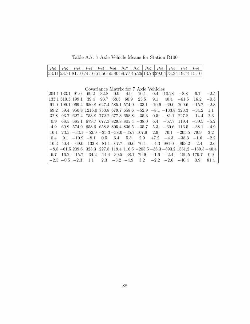
Table A.7: 7 Axle Vehicle Means for Station R100

µp1 µp2 µp3 µp4 µp5 µp6 µp7 µs1 µs2 µs3 µs4 µs5 µs653.11 53.71 81.10 74.16 61.56 60.80 59.77 45.26 13.73 29.04 73.34 19.74 15.10

Covariance Matrix for 7 Axle Vehicles

204.1 133.1 91.0 69.2 32.8 0.9 4.9 10.1 0.4 10.28 −8.8 6.7 −2.5133.1 510.3 199.1 39.4 93.7 68.5 60.9 23.5 9.1 40.4 −61.5 16.2 −0.591.0 199.1 969.4 950.8 627.4 585.1 574.9 −33.1 −10.9 −69.0 209.6 −15.7 −2.369.2 39.4 950.8 1216.0 753.8 679.7 658.6 −52.9 −8.1 −133.8 323.3 −34.2 1.132.8 93.7 627.4 753.8 772.2 677.3 658.8 −35.3 0.5 −81.1 227.8 −14.4 2.30.9 68.5 585.1 679.7 677.3 829.8 805.4 −38.0 6.4 −67.7 119.4 −39.5 −5.24.9 60.9 574.9 658.6 658.8 805.4 836.5 −35.7 5.3 −60.6 116.5 −38.1 −4.910.1 23.5 −33.1 −52.9 −35.3−38.0−35.7 107.9 2.9 70.1 −205.5 79.9 3.20.4 9.1 −10.9 −8.1 0.5 6.4 5.3 2.9 47.2 −4.3 −38.3 −1.6 −2.210.3 40.4 −69.0−133.8−81.1−67.7−60.6 70.1 −4.3 981.0 −893.2 −2.4 −2.6−8.8 −61.5 209.6 323.3 227.8 119.4 116.5 −205.5−38.3−893.2 1551.2 −159.5−40.46.7 16.2 −15.7 −34.2 −14.4−39.5−38.1 79.9 −1.6 −2.4 −159.5 179.7 0.9−2.5 −0.5 −2.3 1.1 2.3 −5.2 −4.9 3.2 −2.2 −2.6 −40.4 0.9 81.4

88

Table A.8: 2 Axle Vehicle Means for Station X249

µp1 µp2 µs15.71 18.28 42.94

Table A.9: 3 Axle Vehicle Means for Station X249

µp1 µp2 µp3 µs1 µs247.03 45.79 40.33 48.84 25.97

Covariance Matrix for 2 Axle Vehicles151.3 201.1 45.7201.1 362.1 75.345.7 75.3 68.5

Covariance Matrix for 3 Axle Vehicles

214.5 187.2 193.2 55.2 −113.2187.2 542.0 439.9 36.9 −4.5193.2 439.9 490.9 27.5 −99.055.2 36.97 27.5 139.1 −145.9−113.2 −4.5 −99.0−145.9 524.1

Covariance Matrix for 4 Axle Vehicles

228.1 176.3 256.8 236.3 24.8 −70.5 38.6176.3 407.0 229.6 178.1 14.2 185.8 −20.1256.8 229.6 513.0 440.4 24.9 −288.0 46.5236.3 178.1 440.4 457.6 5.7 −237.7 25.224.8 14.2 24.9 5.7 55.8 −74.9 47.8−70.5 185.8 −288.0−237.7−74.9 1063.7 −266.838.6 −20.1 46.5 25.2 47.8 −266.8 335.7

Table A.10: 4 Axle Vehicle Means for Station X249

µ1 µ2 µ3 µ4 µs1 µs2 µs336.56 42.05 29.12 28.46 39.11 69.13 16.17

89

Table A.11: 5 Axle Vehicle Means for Station X249

µp1 µp2 µp3 µp4 µp5 µs1 µs2 µs3 µs444.14 44.06 42.47 37.13 37.16 46.77 16.01 88.22 17.06

Covariance Matrix for 5 Axle Vehicles

97.9 81.5 84.0 76.6 77.7 18.9 −15.7 30.4 −8.581.5 451.7 434.5 409.9 415.5 1.0 19.3 −32.9 21.084.0 434.5 458.4 417.8 427.0 7.4 −17.8 9.5 −7.876.6 409.9 417.8 484.0 477.2 2.8 −15.1 4.6 −0.277.7 415.5 427.0 477.2 503.9 4.0 −27.3 19.4 −14.718.9 1.0 7.4 2.8 4.0 65.6 −26.5 50.3 −13.0−15.7 19.3 −17.8−15.1−27.3−26.5 154.8 −184.7 132.030.4 −32.9 9.5 4.6 19.4 50.3 −184.7 342.5 −169.5−8.5 21.0 −7.8 −0.2 14.7 −13.0 132.0 −169.5 171.1

Table A.12: 6 Axle Vehicle Means for Station X249

µp1 µp2 µp3 µp4 µp5 µp6 µs1 µs2 µs3 µs4 µs546.49 56.73 56.30 42.65 41.79 41.49 48.43 15.0 66.76 23.87 20.74

Covariance Matrix for 6 Axle Vehicles

188.6 215.9 245.1 150.0 114.8 132.9 63.9 23.1 −124.1 123.7 −72.4215.9 718.1 697.7 382.1 412.9 442.0 91.5 −1.2 −122.2 120.4 −178.6245.1 697.7 794.3 452.2 446.9 478.7 104.6 −68.0−143.8 181.1 −186.4150.0 382.1 452.2 484.4 363.8 359.6 0.6 −44.7−105.7 124.9 −24.4114.8 412.9 446.9 363.8 450.5 433.1 20.9 −44.2 −0.5 15.33 −46.8132.9 442.0 478.7 359.6 433.1 483.3 36.9 −43.9 −19.2 30.6 −84.563.9 91.5 104.6 30.6 20.9 36.9 89.9 −16.3 −57.9 71.8 −104.2−23.1 −1.2 −68.0 −44.7 −44.2−43.9 −16.3 153.0 −91.1 −14.0 −15.8−124.1−122.2−143.8−105.7 −0.5 −19.2 −57.9 −91.1 737.7 −455.0 −37.7123.7 120.4 181.1 124.9 15.3 30.6 71.8 −14.0−455.0 407.0 32.2−72.4 −178.6−186.4 −24.4 −46.8−84.5−104.2−15.8 −37.7 32.2 368.1

90

Table A.13: 7 Axle Vehicle Means for Station X249

µp1 µp2 µp3 µp4 µp5 µp6 µp7 µs1 µs2 µs3 µs4 µs5 µs649.75 59.22 73.67 59.98 47.33 46.71 46.28 49.58 17.45 32.65 67.58 15.80 14.06

Covariance Matrix for 7 Axle Vehicles

285.0 196.5 193.9 102.0 36.6 16.2 27.8 60.6 −11.3 −17.0 6.6 0.7 −1.7196.5 781.0 413.6 74.5 73.2 61.6 77.0 58.1 −5.5 −22.0 2.9 −4.8 −0.9193.9 413.6 881.3 684.1 461.6 449.3 427.9 13.9 −31.4 −47.8 118.7 5.2 9.9102.0 74.5 684.1 926.8 592.1 570.2 530.7 −37.8 −13.0 −30.3 126.7 1.8 9.536.6 73.2 461.6 592.1 613.1 531.9 485.1 −49.2 −4.3 0.8 66.5 3.9 6.816.2 61.6 449.3 570.2 531.9 547.8 501.3 −50.4 −5.5 −3.8 67.8 7.2 7.227.8 77.0 427.9 530.7 485.1 501.3 516.4 −48.4 −13.2 −0.5 70.7 7.7 6.460.6 58.1 13.9 −37.8−49.2−50.4−48.4 198.1 −28.0 −24.7 −89.4 17.2 −0.6−11.3 −5.5 −31.4−13.0 −4.3 −5.5 −13.2−28.0 348.3 −95.3 −213.9 −19.0 −13.8−17.0−22.0−47.8−30.3 0.8 −3.8 −0.5 −24.7 −95.3 1306.8 −1014.5 51.5 −6.26.6 2.9 118.7 126.7 66.5 67.8 70.7 −89.4−213.9−1014.5 1482.6 −110.9 2.90.7 −4.8 .2 1.8 3.9 7.2 7.7 17.2 −19.0 51.5 −110.9 178.8 13.8−1.7 −0.9 9.9 9.5 6.8 7.2 6.4 −0.6 −13.8 −6.2 2.9 13.8 54.9

91

Table A.14: 2 Axle Vehicle Means for Station G005

µp1 µp2 µs17.99 22.69 42.61

Table A.15: 3 Axle Vehicle Means for Station G005

µp1 µp2 µp3 µs1 µs251.55 51.59 46.74 47.89 20.81

Covariance Matrix for 2 Axle Vehicles167.7 250.7 57.5250.7 515.1 118.857.5 118.8 98.5

Covariance Matrix for 3 Axle Vehicles

279.4 291.5 313.1 22.1 −111.9291.5 932.2 833.0 −9.0 1.1313.1 833.0 883.2 −20.0 −77.122.1 −9.0 −20.0 91.5 −79.1−111.9 1.1 −77.1−79.1 401.0

Covariance Matrix for 4 Axle Vehicles

392.6 219.4 542.6 505.6 4.3 −265.2 40.9219.4 592.7 300.4 265.2 −2.1 225.0 2.7542.6 300.4 1084.1 1009.3 −12.2−606.2 50.6505.6 265.2 1009.3 1022.8 −27.9−554.7 47.44.3 −2.1 −12.2 −27.9 32.1 −21.6 16.8−265.2 225.0−606.2−554.7−21.6 1190.0 −162.5

40.9 2.7 50.6 47.4 16.8 −162.5 186.9

Table A.16: 4 Axle Vehicle Means for Station G005

µ1 µ2 µ3 µ4 µs1 µs2 µs340.47 48.21 38.66 37.19 37.67 63.72 14.09

92

Table A.17: 5 Axle Vehicle Means for Station G005

µp1 µp2 µp3 µp4 µp5 µs1 µs2 µs3 µs445.86 49.21 46.72 41.30 41.13 43.91 16.18 84.13 16.88

Table A.18: 6 Axle Vehicle Means for Station G005

µp1 µp2 µp3 µp4 µp5 µp6 µs1 µs2 µs3 µs4 µs549.98 66.04 65.13 51.10 51.98 50.93 47.60 13.06 67.29 17.23 15.11

Covariance Matrix for 5 Axle Vehicles

104.2 88.1 90.1 79.0 ∗ 77.9 20.1 −21.0 21.0 −7.188.1 598.7 567.4 563.2 556.2 5.5 25.0 −55.7 31.090.1 567.4 574.8 562.4 560.0 12.1 −19.7 2.8 −5.779.0 563.2 562.4 692.6 670.8 9.5 −25.7 8.8 −13.777.9 556.2 560.0 670.8 689.5 10.7 −38.6 31.9 −32.220.1 5.5 12.1 9.5 10.7 55.7 −25.4 47.4 −13.3−21.0 25.0 −19.7 −25.7 −38.6−25.4 169.4 −209.7 144.721.0 −55.7 2.8 8.8 31.9 47.4 −209.7 390.1 −196.4−7.1 31.0 −5.7 −13.7 −32.2−13.3 144.7 −196.4 185.2

Covariance Matrix for 6 Axle Vehicles

160.5 53.7 59.8 67.3 43.0 21.6 7.0 −0.4 −79.3 33.7 3.753.7 812.7 787.1 600.4 629.7 632.2 23.0 −3.5 39.5 −5.2 −39.359.8 787.1 812.4 621.8 636.3 634.7 24.0 −5.4 10.2 24.5 −41.967.4 600.4 621.8 802.8 645.2 581.8 −10.7−4.0 −80.7 28.8 13.043.0 629.7 636.3 645.2 799.9 740.2 −16.6−3.2 −75.8 −1.8 11.521.6 632.2 634.7 581.8 740.2 783.6 −3.8 −3.2 −48.8 −7.6 −5.27.0 23.0 24.0 −10.7−16.6 −3.8 0.9 0.3 9.9 15.9 −20.1−0.4 −3.5 −5.4 −4.0 −3.2 −3.2 0.3 4.4 −3.2 0.1 0.1−79.3 39.5 10.2 −80.7−75.8−48.8 9.9 −3.2 389.2 −119.5−36.733.7 −5.2 24.5 28.8 −1.8 −7.6 15.9 0.1 −119.5 109.2 15.63.7 −39.3−41.9 13.0 11.5 −5.2 −20.1 0.1 −36.7 15.6 66.2

93

Table A.19: 7 Axle Vehicle Means for Station G005

µp1 µp2 µp3 µp4 µp5 µp6 µp7 µs1 µs2 µs3 µs4 µs5 µs647.36 55.53 82.94 70.21 63.43 63.32 62.01 43.66 13.27 34.55 63.71 18.46 14.79

Covariance Matrix for 7 Axle Vehicles

152.1 29.3 76.2 74.1 9.9 −4.4 −4.4 9.1 −3.2 −0.4 20.0 −4.1 −2.929.3 597.4 163.4 −127.0 120.7 109.2 143.7 16.5 −3.3 9.7 −94.7 23.5 −1.176.2 163.4 751.9 643.9 428.8 441.1 428.7 −65.5 −20.2 −169.9 199.7 −47.8 −8.074.1 −127.0 643.9 1020.3 510.7 531.4 488.8 −99.3 −17.3 −255.9 306.3 −69.8 −7.89.9 120.7 428.8 510.7 654.4 612.0 596.2 −64.4 −18.8 −184.8 142.6 −46.3 0.8−4.4 109.2 441.1 531.4 12.0 660.8 630.6 −66.4 −19.1 −180.3 149.4 −49.2 1.4−4.4 143.7 428.7 488.8 596.2 630.6 652.3 −62.2 −17.4 −163.2 119.7 −45.0 2.39.1 16.5 −65.5 −99.3 −64.4 −66.4 −62.2 86.7 2.1 180.3 −205.8 80.3 26.2−3.2 −3.3 −20.2 −17.3 −18.8 −19.1 −17.4 2.1 38.1 6.8 −49.3 −1.9 −0.8−0.4 9.7 −169.9−255.9−184.8−180.3−163.2 180.3 6.8 967.4 −1007.3 165.7 27.020.0 94.7 199.7 306.3 142.6 149.4 119.7 −205.8−49.3−1007.3 1583.8 −246.6−40.6−4.1 23.5 −47.8 −69.8 −46.3 49.2 −45.0 80.3 −1.9 165.7 −246.6 327.6 13.3−2.9 −1.1 8.0 −7.8 0.8 1.4 2.3 26.2 0.8 27.0 −40.6 13.3 84.2

94

Table A.20: 2 Axle Vehicle Means for Station R001

µp1 µp2 µs16.70 22.54 44.16

Table A.21: 3 Axle Vehicle Means for Station R001

µp1 µp2 µp3 µs1 µs247.33 50.94 41.12 50.95 21.96

Covariance Matrix for 2 Axle Vehicles186.4 258.3 67.7258.3 536.8 127.967.7 127.9 100.8

Covariance Matrix for 3 Axle Vehicles

313.1 269.7 215.5 100.6 −83.2269.7 842.3 538.2 87.5 41.7215.5 538.2 569.7 16.6 −13.6100.6 87.5 16.6 205.0 −135.1−83.2 41.7 −13.6−135.1 500.5

Covariance Matrix for 4 Axle Vehicles

300.9 249.2 295.7 264.3 −23.5 −8.3 35.4249.2 676.3 365.5 307.5 −21.9 321.0 −84.5295.7 365.5 525.1 443.8 −22.8 −74.7 45.3264.3 307.5 443. 473.8 −46.8 −32.5 31.8−23.5−21.9−22.8−46.8 87.0 −81.8 52.6−8.3 321.0 −74.7−32.5−81.8 1012.8 −422.335.4 −84.5 45.3 31.8 52.6 −422.3 465.7

Table A.22: 4 Axle Vehicle Means for Station R001

µ1 µ2 µ3 µ4 µs1 µs2 µs338.03 51.10 32.63 31.13 36.77 70.82 18.23

95

Table A.23: 5 Axle Vehicle Means for Station R001

µp1 µp2 µp3 µp4 µp5 µs1 µs2 µs3 µs444.65 49.32 47.77 43.43 43.04 45.32 12.71 88.60 13.41

Table A.24: Six Axle Vehicle Means for Station R001

µp1 µp2 µp3 µp4 µp5 µp6 µs1 µs2 µs3 µs4 µs546.75 68.36 67.79 48.44 49.0 48.18 47.13 12.99 69.65 15.71 12.70

Covariance Matrix for 5 Axle Vehicles

99.1 91.3 88.2 85.7 84.2 16.4 −0.1 6.4 2.291.3 550.8 530.4 546.2 546.3 23.8 5.4 19.4 10.688.2 530.4 539.6 543.1 544.1 25.1 −2.3 30.7 8.885.7 546.2 543.1 676.8 653.0 27.4 −2.3 29.0 18.684.2 546.3 544.1 653.0 673.8 27.0 −3.0 29.9 15.016.4 23.8 25.1 27.4 27.0 63.6 −1.5 24.2 10.9−0.1 5.4 −2.3 −2.3 −3.0 −1.5 25.8 −24.8 8.26.4 19.4 30.7 29.0 29.9 24.2 −24.8 158.4 −14.92.2 10.6 8.8 18.6 15.0 10.9 8.2 −14.9 37.1

Covariance Matrix for 6 Axle Vehicles

161.9 190.5 206.5 120.3 118.9 127.1 34.9 −2.6 −81.4 57.3 −0.2190.5 1015.0 969.9 661.7 706.7 701.4 38.5 −3.9 −57.2 27.5 −10.8206.5 969.9 1031.6 717.1 728.2 725.1 41.8 −18.9−104.7 76.9 −10.7120.2 661.7 717.1 825.1 649.2 595.1 −5.5 −11.7 −74.1 74.9 8.7118.9 706.7 728.2 649.2 721.8 657.7 −0.3 −12.8 −60.0 42.2 5.0127.1 701.4 725.1 595.1 657.7 709.9 8.6 −13.0 −80.0 52.1 1.134.9 38.5 41.8 −5.5 −0.3 8.6 63.7 0.2 −15.9 21.8 0.2−2.6 −3.9 −18.9 −11.7−12.8−13.0 0.2 37.0 −21.0 1.4 0.3−81.4 −57.2 −104.7−74.1−60.0−80.0−15.9−21.0 357.5 −177.2 −4.557.3. 27.5 76.9 74.9 42.2 52.1 21.8 1.4 −177.2 150.9 9.0−0.2 −10.8 −10.7 8.7 5.0 1.1 0.2 0.3 −4.5 9.0 23.6

96

Table A.25: Seven Axle Vehicle Means for Station R001

µp1 µp2 µp3 µp4 µp5 µp6 µp7 µs1 µs2 µs3 µs4 µs5 µs650.29 63.72 79.09 59.94 57.23 59.29 53.21 43.58 14.72 24.75 61.08 16.83 13.31

Covariance Matrix for 7 Axle Vehicles

241.5 192.2 194.1 129.4 29.7 50.9 91.4 −3.3 4.5 −16.7 −25.2 −4.0 1.4192.2 909.5 420.6 −120.3 220.0 158.6 28.6 17.1 −13.7 −43.4 −13.9 −23.1 −25.1194.1 420.6 831.0 526.6 421.5 452.1 414.8 −16.2 −18.9 −40.8 26.5 −3.2 1.8129.4 −120.3 526.6 1114.4 307.5 398.0 638.8 −19.1 0.1 13.4 95.9 1.9 22.629.7 220.0 421.5 307.5 815.9 534.2 301.0 −26.2 −23.3 −57.6 112.4 −15.5 −11.750.9 158.6 452.1 398.0 534.2 712.4 406.2 −30.4 −18.3 −61.4 60.6 10.8 −1.391.4 28.6 414.8 638.8 301.0 406.2 775.7 −8.6 −4.6 −16.6 65.0 −1.6 12.0−3.3 17.1 −16.2 −19.1 −26.2−30.4 −8.6 123.1 6.5 19.5 −27.1 −10.8 −6.14.5 −13.7 −18.9 0.1 −23.3−18.3 −4.6 −6.5 195.8 −28.2 −122.6 −0.2 1.4−16.7 −43.5 −40.8 13.4 −57.6−61.4−16.6 19.5 −28.2 865.7 −586.1 −26.1 −0.9−25.2 −13.9 26.5 95.9 112.4 60.6 65.0 −27.1−122.6−586.1 1223.6 −192.2−36.2−4.0 −23.1 −3.2 1.9 −15.5 10. −1.6 −10.8 −0.2 −26.1 −192.2 224.8 3.21.4 −25.1 1.8 22.6 −11.7 −1.3 12.0 −6.1 1.4 −0.9 −36.3 3.2 98.2

97

Appendix B: Cross Sections ofSuperstructuresDesigned usingAASHTO LRFD

2.5’ 2.5’ 9.17’ 9.17’ 9.17’ 1.5’ 1.5’

3’ 0.75’

W 24x84 (typ.)

Slab Reinforcement: #6 @ 3” primary #4 @ 6” transverse

Figure B.1: 10m Bridge Superstructure Cross Section

98

2.5’ 2.5’ 9.17’ 9.17’ 9.17’ 1.5’ 1.5’

3’ 0.75’

W 40x211 (typ.)

Slab Reinforcement: #6 @ 3” primary, #4 @ 6” transverse

W 40x167 (typ.)

Figure B.2: 20m Bridge Superstructure Cross Section

3’ 0.75’

Slab Reinforcement: #6 @ 3” primary, #4 @ 6” transverse

Built-up Section (typ.)

2.05’ 2.05’

7.1’ 7.1’ 7.1’ 1.5’ 1.5’ 7.1’

2.3’

0.4” 5.25’

0.86”

Figure B.3: 30m Bridge Superstructure Cross Section

99

Appendix C: Bridge Finite El-ement Models

This appendix shows screen captures of the finite element models of samplebridges. The models were used to verify design calculations, as well as todetermine the true proportion of the live load that each girder must support.This was a crucial step for the reliability calculations because the distributionfactors calculated using the AASHTO Specifications use the lever rule, whichgives a conservative estimate of this proportion. The lever rule is conservativebecause it does not account for the redundancy due to multiple girders andoverall structure stiffness. The models were formulated using the softwareSAP2000. The parameters that were input include concrete compressivestrength, steel yeild strength, reinforcing steel area, as well as the level ofcomposite action between slab and girders.

100

Figure C.1: Finite Element Model Showing Stress Contours in Slab

101

Figure C.2: Finite Element Model Showing Bendimg Moment Diagram onBeams

102

Appendix D: Fit of MixtureModels to Data

This appendix shows the fitted mixture models plotted over a relative fre-quency histogram of the bending moments produced by all vehicldes in agiven year at the four stations analyzed. The x axis values are bending mo-ments and the y axis represents a probability density or relative frequency.

0 100 200 300 400 500 600 700 800 0

1

2

3

4

5

6

7

8 x 10 -4

0 1000 2000 3000 4000 5000 6000 7000 8000 0

1

2

3

4

5

6 x 10 -4

Figure D.1: Station R100 years 2002 (left) and 2003 (right)

103

0 1000 2000 3000 4000 5000 6000 7000 80000

1

2

3

4

5

6x 10

-4

0 1000 2000 3000 4000 5000 6000 7000 80000

1

2

3

4

5

6x 10

-4

Figure D.2: Station R100 years 2004 (left) and 2005 (right)

0 1000 2000 3000 4000 5000 6000 7000 80000

0.5

1

1.5x 10

-3

0 1000 2000 3000 4000 5000 6000 7000 80000

0.2

0.4

0.6

0.8

1

1.2

1.4x 10

-3

Figure D.3: Station R100 years 2006 (left) and 2007 (right)

0 1000 2000 3000 4000 5000 6000 7000 80000

1

2

3

4

5

6

7

8x 10

-4

0 1000 2000 3000 4000 5000 6000 7000 80000

1

2

3

4

5

6

7

8x 10

-4

Figure D.4: Station R100 years 2008 (left) and 2009 (right)

104

0 1000 2000 3000 4000 5000 6000 7000 80000

1

2

3

4

5

6

7

8x 10

-4

0 1000 2000 3000 4000 5000 6000 7000 80000

1

2

3

4

5

6

7

8x 10

-4

Figure D.5: Station R100 years 2010 (left) and 2011 (right)

0 1000 2000 3000 4000 5000 6000 7000 80000

1

2

3

4

5

6

7

8x 10

-4

0 1000 2000 3000 4000 5000 6000 7000 80000

1

2

3

4

5

6x 10

-4

Figure D.6: Station X249 years 2000 (left) and 2001 (right)

0 1000 2000 3000 4000 5000 6000 7000 80000

1

2

3

4

5

6x 10

-4

0 1000 2000 3000 4000 5000 6000 7000 80000

0.1

0.2

0.3

0.4

0.5

0.6

0.7

0.8

0.9

1x 10

-3

Figure D.7: Station X249 years 2002 (left) and 2003 (right)

105

0 1000 2000 3000 4000 5000 6000 7000 80000

0.2

0.4

0.6

0.8

1

1.2x 10

-3

0 1000 2000 3000 4000 5000 6000 7000 80000

0.1

0.2

0.3

0.4

0.5

0.6

0.7

0.8

0.9

1x 10

-3

Figure D.8: Station X249 years 2004 (left) and 2006 (right)

0 1000 2000 3000 4000 5000 6000 7000 80000

0.1

0.2

0.3

0.4

0.5

0.6

0.7

0.8

0.9

1x 10

-3

0 1000 2000 3000 4000 5000 6000 7000 80000

0.2

0.4

0.6

0.8

1

1.2x 10

-3

Figure D.9: Station X249 years 2007 (left) and 2008 (right)

0 1000 2000 3000 4000 5000 6000 7000 80000

0.2

0.4

0.6

0.8

1

1.2x 10

-3

0 1000 2000 3000 4000 5000 6000 7000 80000

1

2

3

4

5

6

7

8x 10

-4

Figure D.10: Station X249 years 2009 (left) and 2010 (right)

106

0 1000 2000 3000 4000 5000 6000 7000 80000

1

2

3

4

5

6

7

8x 10

-4

Figure D.11: Station X249 year 2011

0 1000 2000 3000 4000 5000 6000 7000 80000

1

2

3

4

5

6

7

8x 10

-4

0 1000 2000 3000 4000 5000 6000 7000 80000

1

2

3

4

5

6x 10

-4

Figure D.12: Station G005 years 2000 (left) and 2001 (right)

0 1000 2000 3000 4000 5000 6000 7000 80000

1

2

3

4

5

6x 10

-4

0 1000 2000 3000 4000 5000 6000 7000 80000

1

2

3

4

5

6x 10

-4

Figure D.13: Station G005 years 2002 (left) and 2003 (right)

107

0 1000 2000 3000 4000 5000 6000 7000 80000

1

2

3

4

5

6x 10

-4

0 1000 2000 3000 4000 5000 6000 7000 80000

1

2

3

4

5

6x 10

-4

Figure D.14: Station G005 years 2004 (left) and 2005 (right)

0 1000 2000 3000 4000 5000 6000 7000 80000

0.2

0.4

0.6

0.8

1

1.2

1.4x 10

-3

0 1000 2000 3000 4000 5000 6000 7000 80000

0.2

0.4

0.6

0.8

1

1.2x 10

-3

Figure D.15: Station G005 years 2006 (left) and 2007 (right)

0 1000 2000 3000 4000 5000 6000 7000 80000

0.2

0.4

0.6

0.8

1

1.2x 10

-3

0 1000 2000 3000 4000 5000 6000 7000 80000

0.2

0.4

0.6

0.8

1

1.2

1.4x 10

-3

Figure D.16: Station G005 years 2008 (left) and 2009 (right)

108

0 1000 2000 3000 4000 5000 6000 7000 80000

0.5

1

1.5

2

2.5x 10

-3

0 1000 2000 3000 4000 5000 6000 7000 80000

0.5

1

1.5

2

2.5

3

3.5

4x 10

-3

Figure D.17: Station G005 years 2010 (left) and 2011 (right)

0 1000 2000 3000 4000 5000 6000 7000 80000

1

2

3

4

5

6x 10

-4

0 1000 2000 3000 4000 5000 6000 7000 80000

1

2

3

4

5

6x 10

-4

Figure D.18: Station R001 years 2000 (left) and 2001 (right)

0 1000 2000 3000 4000 5000 6000 7000 80000

1

2

3

4

5

6x 10

-4

0 1000 2000 3000 4000 5000 6000 7000 80000

1

2

3

4

5

6x 10

-4

Figure D.19: Station R001 years 2002 (left) and 2003 (right)

109

0 1000 2000 3000 4000 5000 6000 7000 80000

1

2

3

4

5

6x 10

-4

0 1000 2000 3000 4000 5000 6000 7000 80000

1

2

3

4

5

6x 10

-4

Figure D.20: Station R001 years 2004 (left) and 2005 (right)

0 1000 2000 3000 4000 5000 6000 7000 80000

1

2

3

4

5

6x 10

-4

0 1000 2000 3000 4000 5000 6000 7000 80000

1

2

3

4

5

6

7

8x 10

-4

Figure D.21: Station R001 years 2006 (left) and 2007 (right)

0 1000 2000 3000 4000 5000 6000 7000 80000

1

2

3

4

5

6

7

8x 10

-4

0 1000 2000 3000 4000 5000 6000 7000 80000

1

2

3

4

5

6

7

8x 10

-4

Figure D.22: Station R001 years 2008 (left) and 2009 (right)

110

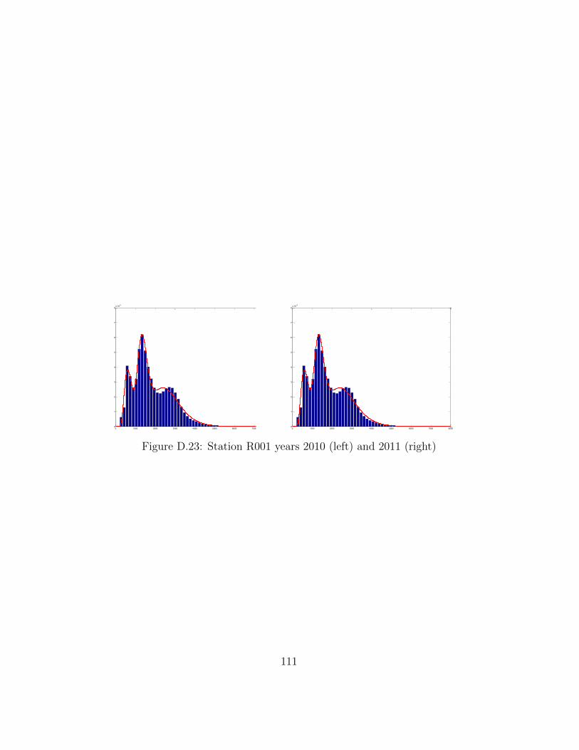
0 1000 2000 3000 4000 5000 6000 7000 80000

1

2

3

4

5

6

7

8x 10

-4

0 1000 2000 3000 4000 5000 6000 7000 80000

1

2

3

4

5

6

7

8x 10

-4

Figure D.23: Station R001 years 2010 (left) and 2011 (right)

111