vermilion river watershed (il basin) tmdl report · 1 1. introduction this report is the third...
TRANSCRIPT

Illinois EnvironmentalProtection Agency
Bureau of WaterP.O. Box 19276Springfield, IL 62794-9276 July 2009
Printed on Recycled Paper
Vermilion River Watershed (IL Basin)TMDL Report
IEPA/BOW/
Vermilion River
§̈¦39
§̈¦55
47
23
116
115
170
18
17
251
179
MCLEAN
LASALLE
LIVINGSTON
FORD
WOODFORD
Pontiac
Streator
Oglesby
Tonica
Minonk
FairburyChenoa Chatsworth
Forrest
Ransom
Cullom
Flanagan
Piper City
Saunemin
Cornell
Illinois River

This page intentionally left blank

i
Table of Contents 1. Introduction ................................................................................................................................................... 1 2. Physical Settings ............................................................................................................................................ 2
2.1. Listed Water Bodies ............................................................................................................................... 2 2.2. Watershed Characteristics ...................................................................................................................... 4
Land Use .................................................................................................................................................... 4 Land Cover ................................................................................................................................................ 5 Soils ........................................................................................................................................................... 8 Hydromodification ..................................................................................................................................... 9 Climate ....................................................................................................................................................... 9 Populations............................................................................................................................................... 11
Humans ........................................................................................................................................... 11 Wildlife ........................................................................................................................................... 11 Pets .................................................................................................................................................. 11 Livestock ......................................................................................................................................... 12
3. Water Quality Standard and Guideline ........................................................................................................ 15 3.1 Nitrogen ................................................................................................................................................. 15
Aquatic Life Use Assessment .................................................................................................................. 15 Public Water Supply Use Assessment ..................................................................................................... 16
3.2 Fecal Coliform Bacteria ........................................................................................................................ 16 Primary Contact Use Assessment ............................................................................................................ 17
4. Description of Water Quality Problem/Impairment .................................................................................... 18 4.1 Vermilion River Segment DS-06 Water Quality Data .......................................................................... 19 4.2. Vermilion River Segment DS-10 Water Quality Data .......................................................................... 24 4.3 Vermilion River Segment DS-14 Water Quality Data .......................................................................... 25 4.4 Vermilion River Tributaries Water Quality Data .................................................................................. 26
5. Assessment of Sources ................................................................................................................................ 28 5.1. Point and Nonpoint Sources .................................................................................................................. 28
Point Sources ........................................................................................................................................... 28 NPDES Permitted Facilities ............................................................................................................ 28 Failing Septic Systems .................................................................................................................... 30 Combined Sewer Overflows ........................................................................................................... 30 Confined Animal Feeding Operations ............................................................................................. 31
Nonpoint Sources ..................................................................................................................................... 32 Failing Septic Systems .................................................................................................................... 32 Land Application of Municipal Waste Biosolids ............................................................................ 32 Pets .................................................................................................................................................. 32 Livestock ......................................................................................................................................... 32 Wildlife ........................................................................................................................................... 32
6. TMDL Development ................................................................................................................................... 33 6.1 Water Quality Duration Curve .............................................................................................................. 33 6.2 TMDL .................................................................................................................................................... 36
Allocations ............................................................................................................................................... 36 Margin of Safety ...................................................................................................................................... 39 Seasonality ............................................................................................................................................... 39 Critical Conditions ................................................................................................................................... 39
7. Public Participation...................................................................................................................................... 40 8. References ................................................................................................................................................... 41

ii
Figures Figure 1. South Fork Vermilion River ................................................................................................................ 1 Figure 2. Kelly Creek ........................................................................................................................................ 2 Figure 3. Segment Map ..................................................................................................................................... 3 Figure 4. Land Use in Vermilion River Watershed ........................................................................................... 6 Figure 5. Barn/Corncrib in Vermilion Watershed ............................................................................................. 6 Figure 6. Corn Tillage in Vermilion Watershed ................................................................................................ 7 Figure 7. Soybean Tillage in Vermilion Watershed .......................................................................................... 7 Figure 8. Soil Orders of the United States ......................................................................................................... 8 Figure 9. North Fork Vermilion Tributary ........................................................................................................ 9 Figure 10. Monthly Precipitation for Pontiac 1996-2005 ................................................................................ 10 Figure 11. Deer Densities (deer per square mile) ............................................................................................ 12 Figure 12. Livestock per County ..................................................................................................................... 13 Figure 13. Livestock Populations per County (Sum of Hogs, Cattle, Sheep, Horses and Chickens) .............. 14 Figure 14. Monitoring Stations in Vermilion Watershed ................................................................................ 18 Figure 15. Fecal Coliform Data for Station DS-06 (1978- 2006) .................................................................... 20 Figure 16. Nitrate Data for Segment DS-06 (1978- 2006) .............................................................................. 21 Figure 17. Nitrate Exceedences in Vermilion River Segment DS-06 (1978-2004) ........................................ 22 Figure 18. Nitrate Monthly Averages for Pontiac's PWS Intake (2002-2007) ................................................ 23 Figure 19. Segment DS-06 Monitoring Stations ............................................................................................. 23 Figure 20. Segment DS-10 Sampling Stations ................................................................................................ 24 Figure 21. Sampling Station for DS-14 ........................................................................................................... 25 Figure 22. Sampling Stations for Vermilion Tributaries ................................................................................. 27 Figure 23. NPDES Facilities in Vermillion Watershed ................................................................................... 28 Figure 24. Combined Sewer Overflows .......................................................................................................... 31 Figure 25. USGS Stream Gages in Vermilion Watershed ............................................................................... 34 Figure 26. Fecal Coliform Duration Curve for DS-06……………………………………..………………...34 Figure 27. Nitrate Duration Curve for DS-06………………………………………………………………..35 Figure 28. Nitrate Duration Curve for DS-10………………………………………………………………..35 Figure 29. Nitrate Duration Curve for DS-14………………………………………………………………..36 Tables Table 1. Impaired Segments in Vermilion Watershed ....................................................................................... 3 Table 2. County Areas within the Vermilion Watershed .................................................................................. 4 Table 3. Land Use in Vermilion River Watershed ............................................................................................ 4 Table 4. Land Cover in Vermilion Watershed ................................................................................................... 5 Table 5. Climate Summary for Pontiac Station 116910 (1971-2000) ............................................................. 10 Table 6. Precipitation for Pontiac Station 116910 (1996-2005) ...................................................................... 10 Table 7. Populations for larger cities ............................................................................................................... 11 Table 8. Deer Populations ............................................................................................................................... 11 Table 9. Livestock Populations by County ...................................................................................................... 13 Table 10. Guidelines for Assessing Primary Contact (Swimming) Use in Illinois Streams ........................... 17 Table 11. Fecal Coliform and Nitrogen Impairments on Current and Previous 303(d) Lists in the Vermilion
Watershed ................................................................................................................................................ 19 Table 12. Fecal Coliform Data for Segment DS-06 (1995-2006) ................................................................... 19 Table 13. Nitrate Data for Station DS-06 on Vermilion River (1997-2006) ................................................... 20 Table 14. Nitrate Monthly Averages for Pontiac's PWS Intake (2002-2007) ................................................. 22 Table 15. Nitrate Data for Segment DS-10 (1990- 2007)................................................................................ 24 Table 16. Sampling Data for Segment DS-14 (1990- 2007) ........................................................................... 25 Table 17. Sampling Data from Vermilion Tributary Segments (1990- 2007) ................................................. 26

iii
Table 18. NPDES Sewage Treatment Facilities in Vermilion Watershed....................................................... 29 Table 19. Untreated Combined Sewer Overflows for Vermilion River Watershed ........................................ 30 Table 20. Treated CSOs in Vermilion Watershed ........................................................................................... 30 Table 21. TMDL Load and Wasteload Allocations ......................................................................................... 37 Table 22. Point Source Wasteloads by Segment ............................................................................................. 38 Table 23. Geometric Means and for Flow Intervals ........................................................................................ 38 Table 24 . Management Practices .................................................................................................................... 39 Appendices Appendix A. Load Calculations for Individual Water Segments Appendix B. TMDL Development from Bottom-up Appendix C. TMDL Implementation Plan for Vermilion River Watershed

iv
This side blank for double-sided printing
1
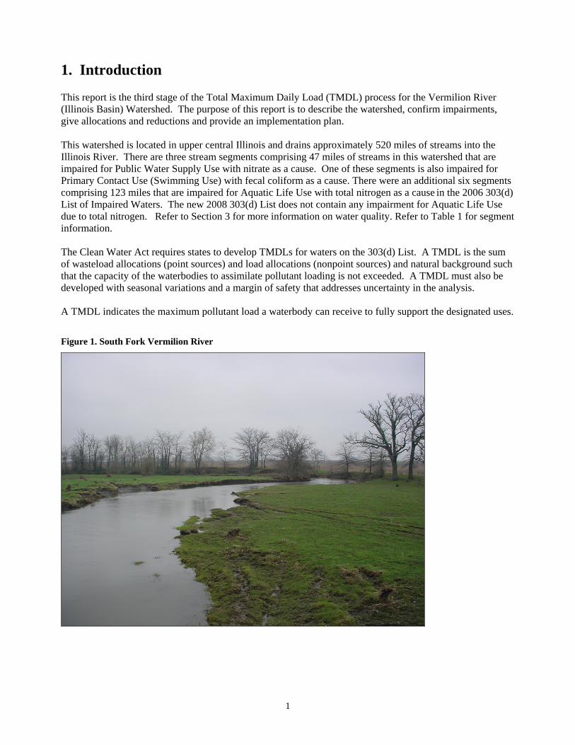
1. Introduction This report is the third stage of the Total Maximum Daily Load (TMDL) process for the Vermilion River (Illinois Basin) Watershed. The purpose of this report is to describe the watershed, confirm impairments, give allocations and reductions and provide an implementation plan. This watershed is located in upper central Illinois and drains approximately 520 miles of streams into the Illinois River. There are three stream segments comprising 47 miles of streams in this watershed that are impaired for Public Water Supply Use with nitrate as a cause. One of these segments is also impaired for Primary Contact Use (Swimming Use) with fecal coliform as a cause. There were an additional six segments comprising 123 miles that are impaired for Aquatic Life Use with total nitrogen as a cause in the 2006 303(d) List of Impaired Waters. The new 2008 303(d) List does not contain any impairment for Aquatic Life Use due to total nitrogen. Refer to Section 3 for more information on water quality. Refer to Table 1 for segment information. The Clean Water Act requires states to develop TMDLs for waters on the 303(d) List. A TMDL is the sum of wasteload allocations (point sources) and load allocations (nonpoint sources) and natural background such that the capacity of the waterbodies to assimilate pollutant loading is not exceeded. A TMDL must also be developed with seasonal variations and a margin of safety that addresses uncertainty in the analysis. A TMDL indicates the maximum pollutant load a waterbody can receive to fully support the designated uses. Figure 1. South Fork Vermilion River
2
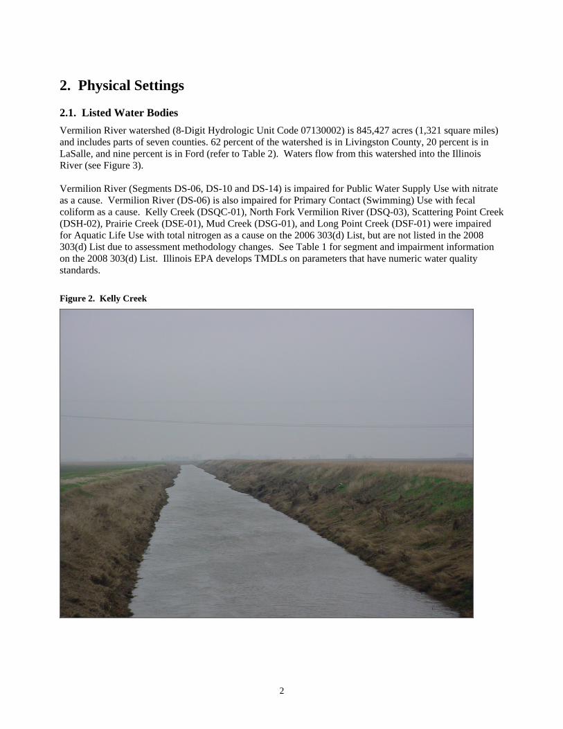
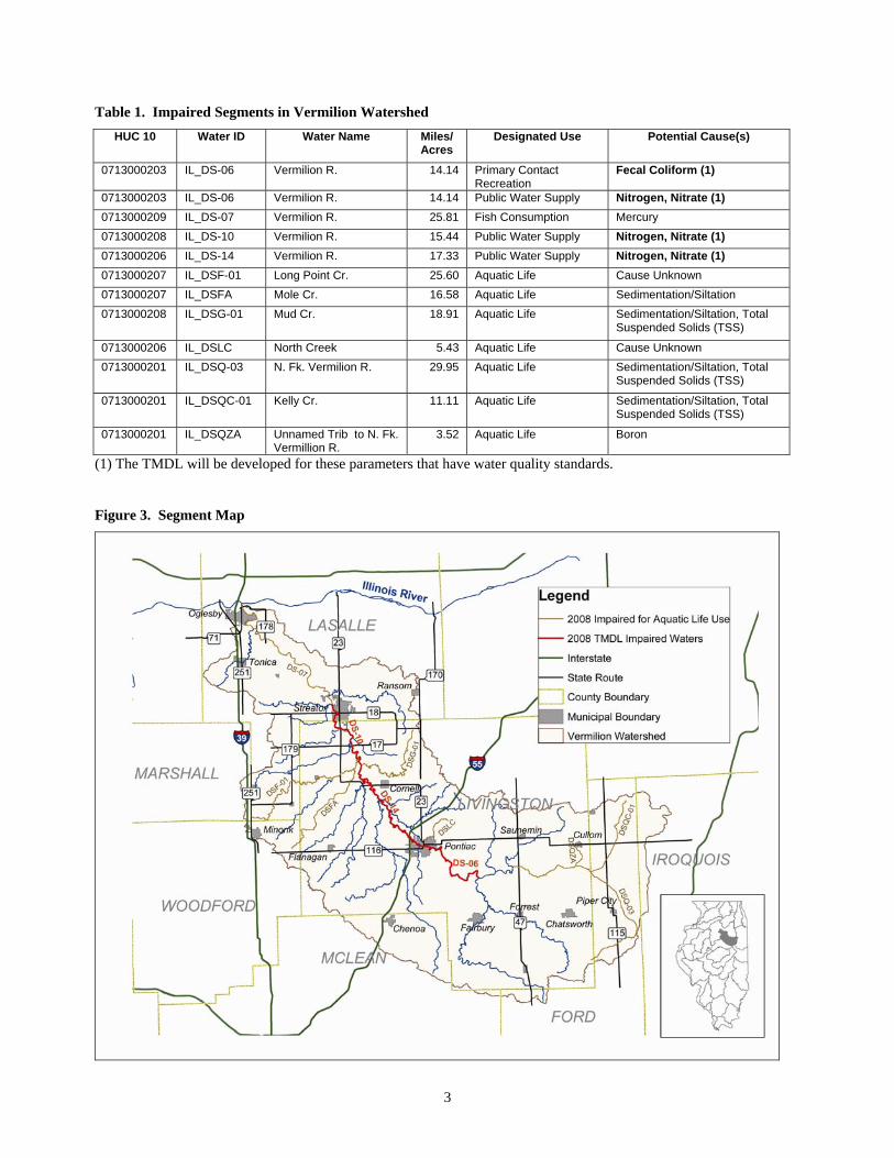
2. Physical Settings 2.1. Listed Water Bodies Vermilion River watershed (8-Digit Hydrologic Unit Code 07130002) is 845,427 acres (1,321 square miles) and includes parts of seven counties. 62 percent of the watershed is in Livingston County, 20 percent is in LaSalle, and nine percent is in Ford (refer to Table 2). Waters flow from this watershed into the Illinois River (see Figure 3). Vermilion River (Segments DS-06, DS-10 and DS-14) is impaired for Public Water Supply Use with nitrate as a cause. Vermilion River (DS-06) is also impaired for Primary Contact (Swimming) Use with fecal coliform as a cause. Kelly Creek (DSQC-01), North Fork Vermilion River (DSQ-03), Scattering Point Creek (DSH-02), Prairie Creek (DSE-01), Mud Creek (DSG-01), and Long Point Creek (DSF-01) were impaired for Aquatic Life Use with total nitrogen as a cause on the 2006 303(d) List, but are not listed in the 2008 303(d) List due to assessment methodology changes. See Table 1 for segment and impairment information on the 2008 303(d) List. Illinois EPA develops TMDLs on parameters that have numeric water quality standards. Figure 2. Kelly Creek
3
Table 1. Impaired Segments in Vermilion Watershed HUC 10 Water ID Water Name Miles/
Acres Designated Use Potential Cause(s)
0713000203 IL_DS-06 Vermilion R. 14.14 Primary Contact Recreation
Fecal Coliform (1)
0713000203 IL_DS-06 Vermilion R. 14.14 Public Water Supply Nitrogen, Nitrate (1) 0713000209 IL_DS-07 Vermilion R. 25.81 Fish Consumption Mercury 0713000208 IL_DS-10 Vermilion R. 15.44 Public Water Supply Nitrogen, Nitrate (1) 0713000206 IL_DS-14 Vermilion R. 17.33 Public Water Supply Nitrogen, Nitrate (1) 0713000207 IL_DSF-01 Long Point Cr. 25.60 Aquatic Life Cause Unknown 0713000207 IL_DSFA Mole Cr. 16.58 Aquatic Life Sedimentation/Siltation 0713000208 IL_DSG-01 Mud Cr. 18.91 Aquatic Life Sedimentation/Siltation, Total
Suspended Solids (TSS)
0713000206 IL_DSLC North Creek 5.43 Aquatic Life Cause Unknown 0713000201 IL_DSQ-03 N. Fk. Vermilion R. 29.95 Aquatic Life Sedimentation/Siltation, Total
Suspended Solids (TSS)
0713000201 IL_DSQC-01 Kelly Cr. 11.11 Aquatic Life Sedimentation/Siltation, Total Suspended Solids (TSS)
0713000201 IL_DSQZA Unnamed Trib to N. Fk. Vermillion R.
3.52 Aquatic Life Boron
(1) The TMDL will be developed for these parameters that have water quality standards.
Figure 3. Segment Map
4
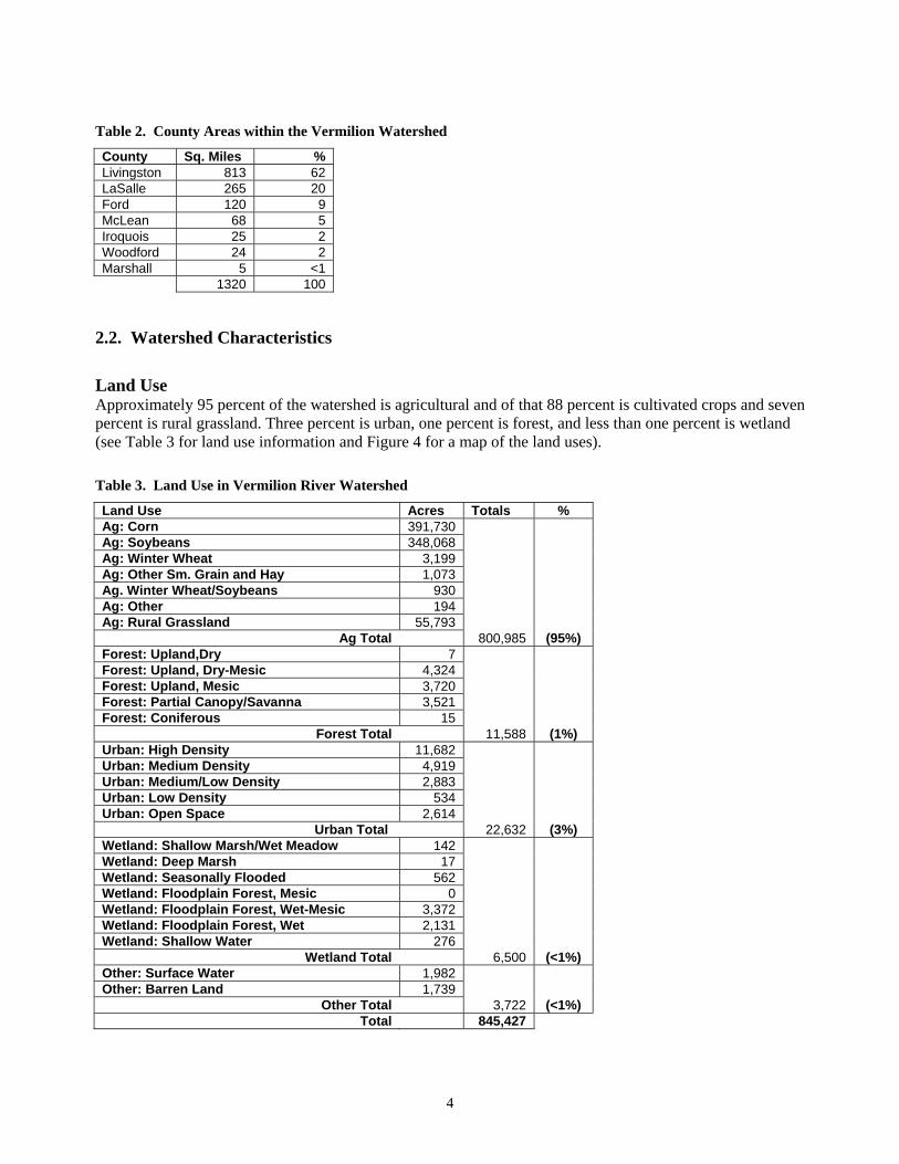
Table 2. County Areas within the Vermilion Watershed
County Sq. Miles % Livingston 813 62 LaSalle 265 20 Ford 120 9 McLean 68 5 Iroquois 25 2 Woodford 24 2 Marshall 5 <1 1320 100
2.2. Watershed Characteristics Land Use Approximately 95 percent of the watershed is agricultural and of that 88 percent is cultivated crops and seven percent is rural grassland. Three percent is urban, one percent is forest, and less than one percent is wetland (see Table 3 for land use information and Figure 4 for a map of the land uses).
Table 3. Land Use in Vermilion River Watershed
Land Use Acres Totals % Ag: Corn 391,730
800,985 (95%)
Ag: Soybeans 348,068 Ag: Winter Wheat 3,199 Ag: Other Sm. Grain and Hay 1,073 Ag. Winter Wheat/Soybeans 930 Ag: Other 194 Ag: Rural Grassland 55,793
Ag Total Forest: Upland,Dry 7
11,588 (1%)
Forest: Upland, Dry-Mesic 4,324 Forest: Upland, Mesic 3,720 Forest: Partial Canopy/Savanna 3,521 Forest: Coniferous 15
Forest Total Urban: High Density 11,682
22,632 (3%)
Urban: Medium Density 4,919 Urban: Medium/Low Density 2,883 Urban: Low Density 534 Urban: Open Space 2,614
Urban Total Wetland: Shallow Marsh/Wet Meadow 142
6,500 (<1%)
Wetland: Deep Marsh 17 Wetland: Seasonally Flooded 562 Wetland: Floodplain Forest, Mesic 0 Wetland: Floodplain Forest, Wet-Mesic 3,372 Wetland: Floodplain Forest, Wet 2,131 Wetland: Shallow Water 276
Wetland Total Other: Surface Water 1,982
3,722 (<1%) Other: Barren Land 1,739
Other Total Total 845,427

5
Land Cover Soil erosion and runoff are greatly affected by land use and land cover. Both affect the infiltration rate. The close proximity of cultivated land to streams creates a high potential for erosion runoff with sediment and pollutants attached to sediment. Since most of the land in the watershed is cultivated row crops, tillage practices were assessed. Tillage practices are available county-wide in the Illinois Department of Agriculture’s 2004 Illinois Soil Conservation Transect Survey Summary. This survey measures the progress in reducing soil erosion to T or tolerable soil loss levels statewide. The tolerable soil loss for most soils is between 3 and 5 tons per acre per year. T is the amount of soil loss that occurs and may be replaced by natural soil-building processes. Reducing soil loss to T is essential to maintaining the long-term agricultural productivity of the soil and to protecting water resources from sedimentation due to soil erosion (IDOA 2004). The survey also includes tillage systems used in planting corn and soybean crops in spring, and small grain crops in fall. Residue left on the fields as a result of reduced tilling is important because it shields the ground from the eroding effects of rain and helps retain moisture for crops. No-till farming leaves the soil virtually undisturbed from harvest through planting. Mulch-till requires at least 30% of the residue from the previous crop to remain on the soil surface after being tilled and planted. Mulch-till and no-till are conservation tillage systems. A Reduced-till system does provide some level of soil conservation; crop residues are not present in the amounts necessary to be categorized as conservation tillage. Conventional tillage does not have any reductions in tilling. Results of the survey are presented in Figure 6 and 7.
From the survey, an average of 91 percent of the points were at or below T or tolerable soil loss levels, seven percent were 1-2T, and one percent were over 2T. Tillage practices varied throughout the watershed. See Figure 6 for corn tillage and Figure 7 for soybean tillage. Table 4. Land Cover in Vermilion Watershed
Corn Tillage (%) Soybean Tillage (%) County %<=1 T 1-2 %T %>2T C R M N C R M N Livingston 89 8 3 66 27 4 3 18 37 16 29 LaSalle 97 3 0 57 42 0 1 5 63 6 26 Ford 85 11 3 85 8 2 5 25 28 10 37 McLean 87 13 0 64 10 14 12 4 8 54 35 Iroquois 94 5 0 65 15 15 5 3 5 55 37 Woodford 95 4 0 19 33 19 9 3 7 30 60 Average 91 7 1
C = Conventional R = Reduced-till M = Mulched-till N = No-till

6
Figure 4. Land Use in Vermilion River Watershed
Figure 5. Barn/Corncrib in Vermilion Watershed

7
Figure 6. Corn Tillage in Vermilion Watershed
Corn Tillage
0102030405060708090
Living
ston
LaSall
eFo
rd
McLea
n
Iroqu
ois
Woodfo
rd
Perc
enta
ge Conventional
Reduced-TillMulch-Till
No-Till
Figure 7. Soybean Tillage in Vermilion Watershed
Soybean Tillage
010203040506070
Living
ston
LaSall
eFo
rd
McLea
n
Iroqu
ois
Woo
dford
Perc
enta
ge Conventional
Reduced-Till
Mulch-Till
No-Till

8
Soils Soils in Illinois were developed when windblown silt called loess was deposited during times of glacial retreat. Melting waters from the retreat carried large amounts of silt, which were deposited along outlets such as the Illinois River. When water subsided, the silt deposits were carried by the wind to the uplands. Winds created the prairies and woodlands developed in the sloped drainage ways. Prairies acted like a sponge that catch and hold rainwater. Illinois is made up of mollisols in the north and alfisols in the south (refer to Figure 8). Mollisols (dark green in the figure) are dark colored soils developed by decomposition of prairie grasses and wildflowers. Alfisols (light green) are light colored and developed under forest vegetation. This area in northern central Illinois is mostly made up of mollisols. Mollisols are very productive agricultural soils and are used extensively for this purpose. Figure 8. Soil Orders of the United States
http://www.nrcs.usda.gov/technical/land/lgif/m4025l.gif

9
Hydromodification Waters in this watershed drain into the Illinois River and then into the Mississippi River. This area of the state is extensively tiled for agricultural purposes to facilitate drainage. When a field is tile-drained, rainwater will move much more rapidly to a watershed outlet when compared to water in the natural soil matrix. Most streams in this watershed are channelized. Channelization straightens, deepens and can widen a stream. Water flows much faster through the altered channel, resulting in increased erosion and flooding downstream. The straightened channel also moves more gravel and sediment downstream. In addition, channelizing can strip streambanks of vegetation, making them more prone to erosion. Natural streams have pools and riffles. Pools help protect streambanks from erosion by absorbing some of the energy of the flowing water. By removing pools, riffles and deep holes, channelizing can harm fish and other aquatic life in the stream. Although channelization may appear to solve a problem in the short term, the stream will constantly work to return to its natural course. This short-term solution can result in long-term problems and high, recurring costs in the watershed.
Figure 9. North Fork Vermilion Tributary
Climate Climate data is from the Illinois State Climatologist Office. Station 116910 is located in Pontiac and was used for climate summaries for the watershed. Figure 3 contains a map showing the city of Pontiac and its central location in the watershed. Table 5 contains the historical temperature and precipitation averages from 1971-2000. Table 6 contains the monthly precipitation data from the last ten years.

10
Table 5. Climate Summary for Pontiac Station 116910 (1971-2000)
Element Jan Feb Mar Apr May Jun Jul Aug Sep Oct Nov Dec AnnHigh °F 30 36 48 62 73 82 85 83 77 65 49 35 60.3Low °F 14 18 29 39 50 60 64 62 54 42 31 20 40.1
Mean °F 22 27 38 50 61 71 74 72 65 53 40 28 50.2Prec. (in) 1.6 1.4 2.8 3.4 3.8 4.1 4.1 3.6 3.0 2.7 3.0 2.5 36.1Snow (in) 9.2 5.5 2.9 0.9 0 0 0 0 0 0 1.7 6.1 26.3
Table 6. Precipitation for Pontiac Station 116910 (1996-2005)
1996 1997 1998 1999 2000 2001 2002 2003 2004 2005 Average
Jan. 1.61 2.27 2.35 3.67 1.29 2.10 2.90 0.43 0.83 4.56 2.20 Feb. 0.62 3.44 2.05 1.11 0.96 2.81 1.75 0.92 0.60 1.75 1.60 Mar. 1.42 1.88 3.86 1.94 1.82 0.86 2.65 2.23 4.41 1.83 2.29 Apr. 2.79 2.35 3.48 5.74 2.87 3.24 4.41 2.12 2.36 1.88 3.12 May 7.58 1.99 3.69 4.40 2.69 3.67 5.58 4.95 5.77 0.66 4.10 Jun. 3.05 2.05 5.84 6.06 4.20 4.83 5.49 2.04 2.25 1.15 3.70 Jul. 6.69 1.27 7.73 2.19 5.16 4.46 2.22 4.83 3.33 1.95 3.98
Aug. 0.68 6.58 1.16 3.14 2.02 3.98 4.38 1.29 4.80 2.97 3.10 Sep. 3.19 2.62 0.92 1.25 3.50 4.06 1.19 3.59 0.82 2.84 2.40 Oct. 2.44 1.39 3.08 1.45 2.40 6.12 1.54 2.16 2.93 0.62 2.41 Nov. 2.25 2.74 1.54 0.68 3.87 2.09 0.95 3.4 4.43 2.53 2.45 Dec. 2.81 1.15 2.04 2.14 1.50 1.46 1.14 1.67 1.78 1.37 1.71 Tot. 35.1 29.7 37.7 33.8 32.3 39.7 34.2 29.6 34.3 24.1 33.06
http://www.sws.uiuc.edu/data/climatedb/data.asp Table 6 does not show a drastic change for precipitation year-to-year, but the monthly precipitation shows variance (Figure 10 shows monthly variations from the last ten years). Precipitation results in surface runoff, which can convey what is on the ground to the streams in both rural and urban areas. Pollutants from nonpoint sources such as livestock, pets or humans can enter the streams when precipitation occurs. Figure 10. Monthly Precipitation for Pontiac 1996-2005
Precipitation (1996-2005)
0.000.501.001.502.002.503.003.504.004.50
Jan. Feb. Mar. Apr. May Jun. Jul. Aug. Sep. Oct. Nov. Dec.
Inch
es

11
Populations Humans Population calculations were calculated based on the U.S. Census tract data. The approximate total population for these watersheds is 61,736. Populations for the larger cities (cities over 2,000) are given in Table 7. Note that the two largest cities of Streator and Pontiac have had very little change over the last ten years. Table 7. Populations for larger cities
City 1990
Census 2000
Census 2005
EstimatePercent Change
Streator 14,121 14,190 13,899 -2% Pontiac 11,428 11,864 11,457 0% Fairbury 3,643 3,968 3,919 +7% Oglesby 3,619 3,647 3,621 0% Minonk 1,982 2,168 2,158 +8%
Wildlife Deer estimates from Illinois Department of Natural are used to represent wildlife populations. Deer populations were divided by the square miles in the watershed to show the densities. Table 8 shows the deer densities for all the counties in this watershed and Figure 11 is a graphic representation of these densities.
Table 8. Deer Populations
County County Deer Populations
County Square Miles
Deer Density (per sq.
mile)
Percent of Watershed in Each County
Deer in Watershed perCounty
Livingston 2459 1137 2.4 79 1943Ford 936 481 1.9 25 234LaSalle 7845 1137 6.9 23 1804McLean 4744 1174 4.0 6 285Woodford 4453 537 8.3 5 223Iroquois 4769 1108 4.3 2 95Marshall 3688 395 9.3 1 37
IDNR 1998
Pets The number of pets was estimated based on the number of households in the watershed. According to the American Veterinary Medical Association, 36% of households have dogs and 32% of households have cats. Per household, there are 1.6 dogs and 2.1 cats. Since not all cats are outdoors, 1 cat per household will be used. Based on population information, there are 23,297 households in the watershed, so there are approximately 13,419 dogs and 7,455 cats.

12
Figure 11. Deer Densities (deer per square mile)
Most of the watershed is in Livingston County which has one of the lowest deer densities at 2.4 deer per square mile. Marshal, LaSalle and Woodford counties have the highest densities, but deer densities in the actual Vermilion watershed are suspected to be much lower. Deer counts are county wide, and most of the forest/wetland areas in this area are near the Illinois River which is outside the Vermilion watershed. For purposes of this TMDL report, we assumed that deer populations are a reliable indicator of wildlife populations. Livestock Livestock estimates are based on the National Agriculture Statistics Service from the United States Department of Agriculture. Table 9 shows countywide livestock statistics for the most recent year data are available, 2002, and Figure 12 is a graph displaying these statistics. Figure 13 is the sum of livestock populations for all counties in this watershed.

13
Table 9. Livestock Populations by County
Hogs and Pigs
Cattle and calves
Chickens Sheep and Lamb
Horses and Ponies
Ford 29,874 5,687 1,516 296 Iroquois 32,137 19,689 1,240 La Salle 16,205 14,753 762 1,543 758Livingston 125,275 6,238 524 541 McLean 92,321 13,122 2,179 759Marshall 10,532 5,944 392 357Woodford 82,337 7,163 1,387
http://www.nass.usda.gov/census/census02/profiles/il/index.htm Figure 12. Livestock per County
0
20000
40000
60000
80000
100000
120000
140000
Ford
Iroqu
ois
La Sall
e
Living
ston
McLea
n
Marsha
ll
Woodfor
d
Qua
ntity
of A
nim
als
Hogs and PigsCattle and calvesChickensSheep and LambHorses and Ponies

14
Figure 13. Livestock Populations per County (Sum of Hogs, Cattle, Sheep, Horses and Chickens)
Livingston County has the highest livestock population of all the counties and it has the largest area in the watershed. As per the 2002 agricultural census data, Livingston County has over 125,000 hogs/pigs in the county.

15
3. Water Quality Standard and Guideline Water quality standards are developed and enforced by the state to protect the "designated uses" of the state's waterways. Illinois’ designated use categories include: Aquatic Life, Primary Contact (Swimming), Secondary Contact, Drinking Water, and Fish Consumption. In the state of Illinois, setting the water quality standards is the responsibility of the Illinois Pollution Control Board (IPCB). This TMDL will deal with the impaired uses of primary contact and public waters supply. 3.1 Nitrogen Nitrogen Nitrate is the cause of impairment for Public Water Supply Use throughout this watershed. Nitrogen was a cause of impairment for Aquatic Life Use throughout the watershed based on the 2006 303(d) List, but is no longer an impairment for this designated use on the 2008 303(d) List. Nitrogen is an essential plant nutrient and is continually cycled among plants, soil, water, and the atmosphere. The principal form of nitrogen found in surface water is in the inorganic form of nitrate. Nitrate in excess of plant needs travels in runoff, leaches through soil or volatizes to the atmosphere. High amounts of nitrate in drinking water can cause methemoglobinemia in humans when nitrate is converted to toxic nitrite, transforming oxygen carrying hemoglobin to non-oxygen carrying methemoglobin. This can result in cyanosis, weakness, rapid pulse, and at high levels, death. Infants are more susceptible because of higher pH in their stomachs. In infants, this is referred to “blue-baby syndrome”. Water quality standards may be developed to protect the most sensitive human populations, infants. High amounts for nitrates in surface water also contribute to eutrophication and excess growth of aquatic plants, which leads to unpleasant odors and insufficient dissolved oxygen for aquatic life (e.g., Gulf Hypoxia). The TMDL is developed for nitrogen nitrate which is currently the cause of impairment for Public Water Supply Use. At the beginning of this TMDL process, nitrogen was a cause of impairment for Aquatic Life Use so a brief discussion of this is below.
Aquatic Life Use Assessment This section applies to the 2006 303(d) Listing. It is no longer impaired for nitrogen on the 2008 List*. For Aquatic Life Use, assessments are based on a combination of biological information and physiochemical water data. The primary biological measures used are the Index of Biotic Integrity for fish (Karr et al. 1986, Smogor et al. 2005) and the Macroinvertebrate Biotic Index (Illinois EPA 1994). Physiochemical water data used include measures of “conventional” parameters, which include nitrogen. If the biological indicators indicate impairment, then the chemical data are used to determine the parameters potentially causing the impairment. The biological indicators provide direct evidence of whether the goal of the water quality standards is being achieved. There is no numeric standard for total nitrogen. For parameters that have no numeric standard, a statistically derived numeric value is used to identify potential causes of impairment. For nitrogen, a numeric threshold based on the 85th percentile statewide value has historically been used as a guideline. This value is derived from all available data from water years 1978 through 1996, at Ambient Water Quality Monitoring stations around the state. The statistical guideline for nitrogen (nitrate + nitrite) in water is 7.8 mg/L. *The following language is from the 2008 Integrated Report and explains why Illinois EPA does not consider nitrogen an impairment of aquatic life use in 2008.
We have stopped using total nitrogen (which appears as nitrogen [total] on the 303[d] list) as a cause of impairment for aquatic life use. We do not have a standard for total nitrogen related to aquatic life. In streams, we typically do not have total nitrogen data. The methods, criteria and the manner in which nitrogen was reported as a cause of impairment of aquatic life use have changed many times over previous assessment cycles. These criteria had never been shown to be related to

16
aquatic life use impairment in any scientific study and had never been used or proposed as water quality standards. Illinois now believes that the criteria by which it placed total nitrogen on previous 303(d) Lists were not scientifically valid. Illinois does not believe that a scientifically valid criterion currently exists for determining when nitrogen is causing an impairment of aquatic life use in this state. While there is some scientific debate over the contribution of nitrogen to nutrient impacts, we believe that nutrient impacts can best be assessed by using criteria for total phosphorus and total phosphorus data are more widely available than nitrogen data. Furthermore, total nitrogen was not listed as a cause of impairment based on any evidence of excessive plant or algal growth. Total nitrogen was only listed as a cause of impairment when biological or other data indicated that aquatic life use was impaired. At that point in the assessment process inappropriate criteria for total nitrogen were used to infer that total nitrogen was a potential cause of that aquatic life use impairment.
Because Illinois now believes that those previous listings of total nitrogen were based on flaws in the listing methodology, we have deleted and delisted total nitrogen as a cause of impairment for all water bodies. However, this delisting will not affect the basis upon which these waters were assessed as impaired and will not cause any waters to be changed to an unimpaired status. Illinois has not placed any water body on the 303(d) List solely because of high levels of total nitrogen. Also, the vast majority of water body segments where total nitrogen was listed as a cause have remained on the 303(d) List even after this cause was deleted because most of the time there are other pollutant causes listed as well. In a few instances, where total nitrogen was the only pollutant cause listed, there was a potential for an entire water body segment to be removed from the 303(d) List. Each of these cases was reviewed carefully to determine whether these segments are impaired by pollutants or pollution.
We will continue to use the water quality standard for total ammonia nitrogen to indicate toxic impacts from ammonia.
Public Water Supply Use Assessment Public and Food Processing Water Supply is only assessed in waters where that use is currently occurring. The assessment of Public and Food Processing Water Supply or PWS use is based on conditions in both untreated and treated water. The following is the guideline for non-supporting PWS use:
For any single parameter in untreated water, 10% or more of the samples exceed the Standard, for water samples collected in 2001 or later; or For any single parameter in treated water, at least one violation of an applicable Maximum Contaminant Level (MCL) occurs during the most recent three years of available data; or The public water supply uses a treatment approach beyond conventional, without which a violation of at least one MCL is expected during the most recent three years of available data.
Nitrate nitrogen is a cause of impairment for public water supplies and the numeric standard is 10 mg/L. 3.2 Fecal Coliform Bacteria Pathogens are the cause of primary contact use impairment for segment DS-06. Pathogens are easily transported by surface water runoff or other discharges into waterbodies. They can infect humans through contaminated fish, skin contact or ingestion of water. Infections due to pathogen-contaminated recreational waters include gastrointestinal, respiratory, eye, ear, nose, throat, and skin diseases (USEPA 1986).
17
Primary contact use is assessed using fecal coliform bacteria, an indicator organism for pathogens. Pathogenic organisms are difficult to identify, but indicator organisms are more easily sampled and measured. Indicator organisms are nonpathogenic bacteria associated with pathogens transmitted by fecal contamination. Fecal coliform bacteria are found in the intestines and feces of warm-blooded animals.
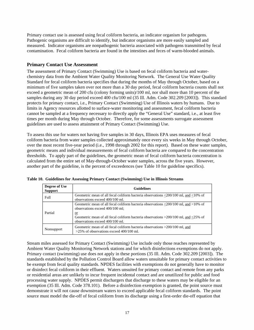
Primary Contact Use Assessment The assessment of Primary Contact (Swimming) Use is based on fecal coliform bacteria and water- chemistry data from the Ambient Water Quality Monitoring Network. The General Use Water Quality Standard for fecal coliform bacteria specifies that during the months of May through October, based on a minimum of five samples taken over not more than a 30 day period, fecal coliform bacteria counts shall not exceed a geometric mean of 200 cfu (colony forming units)/100 ml, nor shall more than 10 percent of the samples during any 30 day period exceed 400 cfu/100 ml (35 Ill. Adm. Code 302.209 [2003]). This standard protects for primary contact, i.e., Primary Contact (Swimming) Use of Illinois waters by humans. Due to limits in Agency resources allotted to surface-water monitoring and assessment, fecal coliform bacteria cannot be sampled at a frequency necessary to directly apply the “General Use” standard, i.e., at least five times per month during May through October. Therefore, for some assessments surrogate assessment guidelines are used to assess attainment of Primary Contact (Swimming) Use. To assess this use for waters not having five samples in 30 days, Illinois EPA uses measures of fecal coliform bacteria from water samples collected approximately once every six weeks in May through October, over the most recent five-year period (i.e., 1998 through 2002 for this report). Based on these water samples, geometric means and individual measurements of fecal coliform bacteria are compared to the concentration thresholds. To apply part of the guidelines, the geometric mean of fecal coliform bacteria concentration is calculated from the entire set of May-through-October water samples, across the five years. However, another part of the guideline, is the percent of exceedences (see Table 10 for guideline specifics). Table 10. Guidelines for Assessing Primary Contact (Swimming) Use in Illinois Streams
Degree of Use Support Guidelines
Full Geometric mean of all fecal coliform bacteria observations <200/100 ml, and <10% of observations exceed 400/100 ml.
Partial
Geometric mean of all fecal coliform bacteria observations <200/100 ml, and >10% of observations exceed 400/100 ml; or Geometric mean of all fecal coliform bacteria observations >200/100 ml, and <25% of observations exceed 400/100 ml.
Nonsupport Geometric mean of all fecal coliform bacteria observations >200/100 ml, and >25% of observations exceed 400/100 ml.
Stream miles assessed for Primary Contact (Swimming) Use include only those reaches represented by Ambient Water Quality Monitoring Network stations and for which disinfections exemptions do not apply. Primary contact (swimming) use does not apply in these portions (35 Ill. Adm. Code 302.209 [2003]). The standards established by the Pollution Control Board allow waters unsuitable for primary contact activities to be exempt from fecal quality standards. NPDES facilities with exemptions do not generally have to monitor or disinfect fecal coliform in their effluent. Waters unsuited for primary contact and remote from any parks or residential areas are unlikely to incur frequent incidental contact and are unutilized for public and food processing water supply. NPDES permit dischargers that discharge to these waters may be eligible for an exemption (35 Ill. Adm. Code 378.101). Before a disinfection exemption is granted, the point source must demonstrate it will not cause downstream waters to exceed applicable fecal coliform standards. The point source must model the die-off of fecal coliform from its discharge using a first-order die-off equation that
18
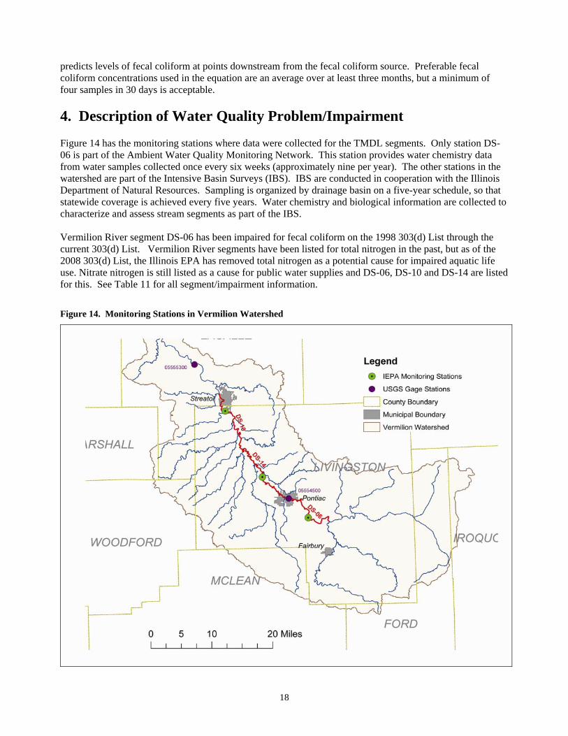
predicts levels of fecal coliform at points downstream from the fecal coliform source. Preferable fecal coliform concentrations used in the equation are an average over at least three months, but a minimum of four samples in 30 days is acceptable. 4. Description of Water Quality Problem/Impairment Figure 14 has the monitoring stations where data were collected for the TMDL segments. Only station DS-06 is part of the Ambient Water Quality Monitoring Network. This station provides water chemistry data from water samples collected once every six weeks (approximately nine per year). The other stations in the watershed are part of the Intensive Basin Surveys (IBS). IBS are conducted in cooperation with the Illinois Department of Natural Resources. Sampling is organized by drainage basin on a five-year schedule, so that statewide coverage is achieved every five years. Water chemistry and biological information are collected to characterize and assess stream segments as part of the IBS. Vermilion River segment DS-06 has been impaired for fecal coliform on the 1998 303(d) List through the current 303(d) List. Vermilion River segments have been listed for total nitrogen in the past, but as of the 2008 303(d) List, the Illinois EPA has removed total nitrogen as a potential cause for impaired aquatic life use. Nitrate nitrogen is still listed as a cause for public water supplies and DS-06, DS-10 and DS-14 are listed for this. See Table 11 for all segment/impairment information. Figure 14. Monitoring Stations in Vermilion Watershed

19
Table 11. Fecal Coliform and Nitrogen Impairments on Current and Previous 303(d) Lists in the Vermilion Watershed
Segment ID Segment Name
Designated Use
1998 2002 2004 2006 2008
IL_DS-06 Vermilion R. Primary Contact
Fecal coliform
Fecal coliform
Fecal coliform
Fecal coliform
Fecal coliform
Aquatic Life Nutrients Total ammonia N
Total nitrogen as N
Public Water Supplies
Nitrate nitrogen
Nitrate nitrogen
Nitrate nitrogen
Nitrate nitrogen
IL_DS-14 Vermilion R. Public Water Supplies
Nitrate nitrogen
Nitrate nitrogen
Nitrate nitrogen
Nitrate Nitrogen
IL_DS-10 Vermilion R. Public Water Supplies
Nitrate nitrogen
Nitrate nitrogen
Nitrate nitrogen
IL_DSE-01 Prairie Cr. Aquatic Life Total nitrogen
IL_DSG-01 Mud Cr. Aquatic Life Total nitrogen
IL_DSF-01 Long Point Cr. Aquatic Life Total nitrogen
IL_DSQC-01
Kelly Cr. Aquatic Life Nutrients Total nitrogen
IL_DSQ-03 N. Fk. Vermilion R.
Aquatic Life Total nitrogen
IL_DSH-02 Scattering Point Cr.
Aquatic Life Total nitrogen
4.1 Vermilion River Segment DS-06 Water Quality Data Seasonal data (May though October) from the last five years for Vermilion River (segment DS-06) have a geometric mean of 148 cfu/100ml and 25 percent of the samples were over 400 cfu/100ml, which makes this segment partially supporting for primary contact (see Table 10 for Primary Contact guidelines). The last ten years of data is included in the table below and all seasonal data (May through October) from 1978 to 2006 are included in Figure 15. Highlighted results are in exceedance of the water quality standard. Table 12. Fecal Coliform Data for Segment DS-06 (1995-2006)
Station Date Parameter Result (cfu/100ml)
DS 06 5/11/1995 FECAL COLIFORM 3900 DS 06 8/10/1995 FECAL COLIFORM 3800 DS 06 5/26/1998 FECAL COLIFORM 266 DS 06 6/23/1998 FECAL COLIFORM 320 DS 06 6/8/1999 FECAL COLIFORM 156 DS 06 7/7/1999 FECAL COLIFORM 131 DS 06 5/4/2000 FECAL COLIFORM 125 DS 06 6/13/2000 FECAL COLIFORM 3800 DS 06 7/24/2000 FECAL COLIFORM 200 DS 06 10/10/2000 FECAL COLIFORM 38 DS 06 10/11/2001 FECAL COLIFORM 33 DS 06 5/13/2002 FECAL COLIFORM 1300 DS 06 8/6/2002 FECAL COLIFORM 90 DS 06 9/19/2002 FECAL COLIFORM 20 DS 06 5/27/2003 FECAL COLIFORM 57

20
Station Date Parameter Result (cfu/100ml)
DS 06 6/25/2003 FECAL COLIFORM 200 DS 06 9/15/2003 FECAL COLIFORM 200 DS 06 10/29/2003 FECAL COLIFORM 20 DS 06 5/20/2004 FECAL COLIFORM 1000 DS 06 7/1/2004 FECAL COLIFORM 190 DS 06 8/12/2004 FECAL COLIFORM 170 DS 06 9/16/2004 FECAL COLIFORM 190 DS-06 10/25/05 FECAL COLIFORM 73 DS-06 05/02/06 FECAL COLIFORM 600 DS-06 06/12/06 FECAL COLIFORM TNTC* DS-06 08/09/06 FECAL COLIFORM 400
*TNTC- Too numerous to count Figure 15. Fecal Coliform Data for Station DS-06 (1978- 2006)
Seasonal Data- May through October
0
500
1000
1500
2000
2500
3000
3500
4000
1/23
/197
8
1/23
/198
0
1/23
/198
2
1/23
/198
4
1/23
/198
6
1/23
/198
8
1/23
/199
0
1/23
/199
2
1/23
/199
4
1/23
/199
6
1/23
/199
8
1/23
/200
0
1/23
/200
2
1/23
/200
4
1/23
/200
6
cfu/
100
ml
Data
GeometricMeanStandard
InstantaneousStandard
DS-06 is also impaired for nitrate. The public water supply use standard for nitrate is 10 mg/L. Data from the last ten years is in the table below and data from 1978 through 2006 are shown in Figure 12. Highlighted results are in exceedance of the water quality standard. Table 13. Nitrate Data for Station DS-06 on Vermilion River (1997-2006)
Station Date Parameter Result (mg/L) DS-06 3/4/1997 Nitrate 11.10 DS-06 4/9/1997 Nitrate 10.40 DS-06 5/21/1997 Nitrate 8.90 DS-06 6/18/1997 Nitrate 13.40 DS-06 7/23/1997 Nitrate 0.93 DS-06 9/25/1997 Nitrate 0.01 DS-06 11/20/1997 Nitrate 0.14
Station Date Parameter Result (mg/L) DS-06 1/12/1998 Nitrate 11.40 DS-06 2/9/1998 Nitrate 10.00 DS-06 3/23/1998 Nitrate 10.00 DS-06 4/24/1998 Nitrate 13.58 DS-06 5/26/1998 Nitrate 13.02 DS-06 6/23/1998 Nitrate 13.40 DS-06 8/19/1998 Nitrate 0.60

21
Station Date Parameter Result (mg/L) DS-06 9/16/1998 Nitrate 0.05 DS-06 10/28/1998 Nitrate 0.25 DS-06 12/11/1998 Nitrate 0.60 DS-06 2/5/1999 Nitrate 12 DS-06 3/17/1999 Nitrate 13 DS-06 4/14/1999 Nitrate 11 DS-06 6/8/1999 Nitrate 15 DS-06 7/7/1999 Nitrate 9.8 DS-06 8/4/1999 Nitrate 0.05 DS-06 9/13/1999 Nitrate 0.18 DS-06 11/9/1999 Nitrate 0.21 DS-06 12/13/1999 Nitrate 0.94 DS-06 1/26/2000 Nitrate 1.04 DS-06 3/2/2000 Nitrate 1.07 DS-06 4/17/2000 Nitrate 1.16 DS-06 5/4/2000 Nitrate 14 DS-06 6/13/2000 Nitrate 14 DS-06 7/24/2000 Nitrate 7.5 DS-06 10/10/2000 Nitrate 0.16 DS-06 11/3/2000 Nitrate 0.38 DS-06 1/24/2001 Nitrate 5.8 DS-06 3/6/2001 Nitrate 14 DS-06 4/2/2001 Nitrate 13 DS-06 4/24/2001 Nitrate 14 DS-06 6/11/2001 Nitrate 15 DS-06 7/23/2001 Nitrate 4 DS-06 11/28/2001 Nitrate 8.1 DS-06 1/22/2002 Nitrate 8.7 DS-06 2/20/2002 Nitrate 12
Station Date Parameter Result (mg/L) DS-06 4/16/2002 Nitrate 13 DS-06 5/13/2002 Nitrate 8.7 DS-06 6/25/2002 Nitrate 11.6 DS-06 8/6/2002 Nitrate 5.17 DS-06 9/19/2002 Nitrate 0.86 DS-06 3/11/2004 Nitrate 12.60 DS-06 4/21/2004 Nitrate 11.70 DS-06 5/20/2004 Nitrate 17.20 DS-06 7/1/2004 Nitrate 9.70 DS-06 11/3/2004 Nitrate 10.80 DS-06 12/14/2004 Nitrate 11.70 DS-06 1/20/2005 Nitrate 10.30 DS-06 3/1/2005 Nitrate 11.90 DS-06 3/21/2005 Nitrate 9.65 DS-06 5/16/2005 Nitrate 8.87 DS-06 6/14/2005 Nitrate 4.03 DS-06 7/25/2005 Nitrate 5.83 DS-06 9/12/2005 Nitrate 0.03 DS-06 12/7/2005 Nitrate 10.20 DS-06 5/2/2006 Nitrate 16.70 DS-06 6/12/2006 Nitrate 13.20 DS-06 8/9/2006 Nitrate 2.18 DS-06 9/14/2006 Nitrate 2.12 DS-06 10/30/2006 Nitrate 8.57 DS-06 12/14/2006 Nitrate 11.50
Figure 16. Nitrate Data for Segment DS-06 (1978- 2006)
0.00
5.00
10.00
15.00
20.00
25.00
1/23
/197
8
1/23
/198
0
1/23
/198
2
1/23
/198
4
1/23
/198
6
1/23
/198
8
1/23
/199
0
1/23
/199
2
1/23
/199
4
1/23
/199
6
1/23
/199
8
1/23
/200
0
1/23
/200
2
1/23
/200
4
1/23
/200
6
mg/
L
DataStandard
From 1978 to 2006, 40 percent of the total samples violate the water quality standard of 10 mg/L (101 out of 245 samples). Figure 17 displays the number of exceedences per month for all data.

22
Figure 17. Nitrate Exceedences in Vermilion River Segment DS-06 (1978-2004)
02468
101214161820
Janu
ary
Febr
uary
March
April
MayJu
ne July
Augus
t
Septem
ber
Octobe
r
Novem
ber
Decem
ber
No. o
f Exc
eede
nces
Nitrate data from June of 2002 through May of 2007 was obtained for the public waters supply intake in Pontiac. Daily data was collected and monthly averages are shown in Table 14 and Figure 18. Table 14. Nitrate Monthly Averages for Pontiac's PWS Intake (2002-2007)
2002 2003 2004 2005 2006 2007 January 2.62 10.11 10.26 10.68 12.56 February 5.37 8.40 13.76 10.73 11.53 March 3.66 11.34 13.37 11.72 8.93 April 8.72 12.74 12.97 15.10 13.17 May 11.82 15.11 9.90 17.07 13.09 June 12.75 12.20 14.78 4.70 13.65 July 9.22 9.23 8.04 0.81 8.51 August 2.98 3.39 2.01 0.89 3.94 September 3.76 0.66 2.10 0.32 3.63 October 1.85 0.55 1.45 0.46 6.25 November 1.24 4.40 10.32 0.71 9.37 December 1.35 11.29 12.03 7.38 11.89

23
Figure 18. Nitrate Monthly Averages for Pontiac's PWS Intake (2002-2007)
0.00
2.00
4.00
6.00
8.00
10.00
12.00
14.00
16.00
18.00
Janu
ary
Februa
ryMarc
hApri
lMay
June Ju
ly
Augus
t
Septem
ber
Octobe
r
Novembe
r
Decembe
r
200220032004200520062007
Figure 19. Segment DS-06 Monitoring Stations

24
4.2. Vermilion River Segment DS-10 Water Quality Data There are multiple stations that have been sampled for this segment (see Figure 20). Stations DS-ST-A1 through C1 have data samples taken through the Facility-Related Stream Survey (FRSS) Program for the Streator STP facility. For an FRSS, Illinois EPA collects data upstream and downstream of municipal and industrial wastewater treatment facilities to determine impacts on the receiving stream. The other stations are from the Intensive Basin Survey Program. Five out of 13 samples exceed the standard for nitrate at segment DS-10. Table 15. Nitrate Data for Segment DS-10 (1990- 2007)
Date Station Parameter Result (mg/ml)
9/6/1990 DS-10 Nitrate 4.90 9/20/1990 DS-12 Nitrate 0.44 7/19/1999 DS-10 Nitrate 8.5 9/13/1999 DS-10 Nitrate 0.01 7/30/2002 DS-ST-A1 Nitrate 4.88 7/30/2002 DS-ST-C1 Nitrate 4.46 7/30/2002 DS-ST-C2 Nitrate 4.24 7/30/2002 DS-ST-E1 Nitrate 1.55 6/2/2004 DS-10 Nitrate 17.70 4/3/2007 DS-10 Nitrate 11.8
4/18/2007 DS-10 Nitrate 12.4 5/8/2007 DS-10 Nitrate 12.9
5/21/2007 DS-10 Nitrate 10.3 Figure 20. Segment DS-10 Sampling Stations

25
4.3 Vermilion River Segment DS-14 Water Quality Data There are multiple stations that have been sampled in previous years (Table 16). Stations DS-PO-A1 through E1 are data taken through the Facility-Related Stream Surveys (FRSSs) Program for Pontiac STP facility. The other stations are from the Intensive Basin Survey Program. Five out of 14 samples exceeded the standard for nitrate at Segment DS-14. Table 16. Sampling Data for Segment DS-14 (1990- 2007)
Date Station Parameter Result (mg/ml)
8/28/1990 DS 15 Nitrate 7.10 8/29/1990 DS 14 Nitrate 6.40 9/17/1990 DS 13 Nitrate 2.20 9/13/1999 DS-14 Nitrate 0.04 9/3/2002 DS-PO-A1 Nitrate 4.63 9/3/2002 DS-PO-C1 Nitrate 5.09 9/3/2002 DS-PO-C2 Nitrate 5.13 9/3/2002 DS-PO-C3 Nitrate 4.77 9/3/2002 DS-PO-E1 Nitrate 12.9 6/2/2004 DS-14 Nitrate 18.10 4/3/2007 DS-14 Nitrate 11
4/18/2007 DS-14 Nitrate 10.6 5/7/2007 DS-14 Nitrate 11.8
5/21/2007 DS-14 Nitrate 9.55 Figure 21. Sampling Station for DS-14

26
4.4 Vermilion River Tributaries Water Quality Data For more watershed information, Illinois EPA examines the tributary data for Vermilion River. High nitrate in the tributaries is likely a contributing factor to water quality standards for public water supply in downstream waters. There were six tributaries that were on the 2006 303(d) List impaired for aquatic life use with total nitrogen as a cause (see Table 17). The statistical guideline stated nitrate data must not exceed 7.8 mg/L. Highlighted results exceed the standard of 10 mg/L. Table 17. Sampling Data from Vermilion Tributary Segments (1990- 2007)
Segment Stream Date Parameter Result (mg/L)
DSE-01 Prairie Cr. 8/2/1990 Nitrate 17.00 DSE-01 Prairie Cr. 6/2/2004 Nitrate 24.00 DSE-01 Prairie Cr. 7/7/2004 Nitrate 9.70 DSE-01 Prairie Cr. 4/3/2007 Nitrate 17.90 DSE-01 Prairie Cr. 4/18/2007 Nitrate 17.8 DSE-01 Prairie Cr. 5/7/2007 Nitrate 18.8 DSE-01 Prairie Cr. 5/21/2007 Nitrate 16 DSF-01 Long Point Cr. 8/1/1990 Nitrate 18.00 DSF-01 Long Point Cr. 6/2/2004 Nitrate 21.00 DSF-01 Long Point Cr. 7/8/2004 Nitrate 12.00 DSF-01 Long Point Cr. 4/18/2007 Nitrate 17.8 DSF-01 Long Point Cr. 4/30/2007 Nitrate 18.40 DSF-01 Long Point Cr. 5/7/2007 Nitrate 21.7 DSF-01 Long Point Cr. 5/21/2007 Nitrate 17.6 DSG-01 Mud Cr. 8/2/1990 Nitrate 8.30 DSG-01 Mud Cr. 6/2/2004 Nitrate 14.40 DSG-01 Mud Cr. 7/7/2004 Nitrate 8.08 DSG-01 Mud Cr. 4/3/2007 Nitrate 7.25 DSG-01 Mud Cr. 4/18/2007 Nitrate 7.68 DSG-01 Mud Cr. 5/7/2007 Nitrate 8.44 DSG-01 Mud Cr. 5/21/2007 Nitrate 7.02 DSH-01 Scattering Point 8/1/1990 Nitrate 16.00 DSH-01 Scattering Point 6/2/2004 Nitrate 20.60 DSH-01 Scattering Point 7/8/2004 Nitrate 11.60 DSH-01 Scattering Point 4/3/2007 Nitrate 14.40 DSH-01 Scattering Point 4/18/2007 Nitrate 14.6 DSH-01 Scattering Point 5/7/2007 Nitrate 16.5 DSH-01 Scattering Point 5/21/2007 Nitrate 14.1 DSH-01 Scattering Point 6/2/2004 Nitrate 20.90 DSH-01 Scattering Point 7/12/2004 Nitrate 11.80 DSQ-01 N. Fk. Vermilion 6/3/2004 Nitrate 19.00 DSQ-01 N. Fk. Vermilion 4/18/2007 Nitrate 11.1 DSQ-01 N. Fk. Vermilion 5/7/2007 Nitrate 11.8 DSQ-01 N. Fk. Vermilion 5/21/2007 Nitrate 8.47 DSQ-01 N. Fk. Vermilion 9/14/1999 Nitrate 0.01 DSQ-01 N. Fk. Vermilion 9/4/1990 Nitrate 0.01 DSQ-01 N. Fk. Vermilion 4/3/2007 Nitrate 11.80 DSQC-01 Kelly Cr. 6/3/2004 Nitrate 18.90 DSQC-01 Kelly Cr. 4/3/2007 Nitrate 12.2 DSQC-01 Kelly Cr. 4/18/2007 Nitrate 11.9 DSQC-01 Kelly Cr. 5/7/2007 Nitrate 11.9 DSQC-01 Kelly Cr. 5/21/2007 Nitrate 9.14

27
Figure 22. Sampling Stations for Vermilion Tributaries

28
5. Assessment of Sources 5.1. Point and Nonpoint Sources There are point and nonpoint sources of fecal coliform bacteria and nitrate in the Vermilion River watershed. Point sources directly discharge into the water body itself. Nonpoint sources are not as easy to quantify because they do not directly discharge, are not regulated by permits and are dependent on facilitators such as precipitation that results in runoff and tile drainage.
Point Sources NPDES Permitted Facilities Point sources in the watershed include permitted NPDES facilities. These include sewage treatment plants, schools and retirement homes. Facilities that treat sewage are in Figure 23 and Table 18. Facilities with a designed average flow (DAF) over one MGD (million gallons per day) are considered major facilities and are labeled “major” on the map. There are two major facilities in this watershed- Pontiac Sewage Treatment Plant and Streator Sewage Treatment Plant. Streator STP discharges downstream of the DS-10 station. On Table 18, the last three columns show which stream the facility discharges in or tributary to. Figure 23. NPDES Facilities in Vermillion Watershed

29
Table 18. NPDES Sewage Treatment Facilities in Vermilion Watershed
NPDES ID Facility Name DAF DMF Exemption (Year)
Parameters Monitored
DS-06
DS-14
DS-10
ILG580091 Chatsworth STP 0.18 0.46 YR (1989) CBOD, SS, pH x x x IL0037001 Greenbriar Health Care 0.01 0.03 YR (1989) CBOD, SS, pH,
ammonia x x x
IL0021601 Fairbury STP 0.66 1.65 YR (1988) CBOD, SS, pH, DO, ammonia
x x x
IL0028819 Forrest STP 0.35 0.88 YR (1988) CBOD, SS, pH, DO
x x x
IL0026697 Stelle Community Assn STP
0.02 0.04 CBOD, SS, pH, DO, ammonia, Cl, fecal coliform
x x x
IL0030457 Pontiac STP 3.50 8.50 S (1994) CBOD, SS, pH, DO, ammonia, Cl, fecal coliform
x x
ILG582009 Chenoa STP 0.26 0.66 YR (1989) CBOD, SS, pH x ILG580057 Flanagan STP 0.13 0.32 YR (1989) CBOD, SS, pH x ILG551069 IL DOT-I-55 Livingston
Co 0.02 0.47 YR (1996) CBOD, SS, pH x
ILG551020 Meadows Mennonite Retirement
0.05 0.11 YR (1990) CBOD, SS, pH x
IL0037818 Minonk STP 0.34 0.85 YR (1989) CBOD, SS, pH, DO
x
IL0024996 Oglesby STP 0.879 1.224 S (1989) CBOD, SS, pH, fecal coliform, chlorine, ammonia
DS
ILG551038 Salem Childrens Home 0.01 0.03 S (1992) CBOD, SS, pH x IL0022004 Streator STP* 3.30 10.80 S (1989) CBOD, SS, pH,
DO ammonia, Cl, fecal coliform, silver
DS
IL0048828 Woodland School 0.01 0.03 YR (1994) CBOD, SS, pH, DO, ammonia
x
S= Seasonal Exemption YR= Year Round Exemption DAF= Daily Average Flow DMF= Daily Maximum Flow DS= Downstream *Streator facility discharges on segment DS-10, but downstream of DS-10 monitoring station. This table contains the parameters that the facility is required to monitor under their NPDES permit. Each discharger is required to submit data to Illinois EPA. Most of the facilities have an exemption from chlorination. Facilities with year-round exemptions do not have to chlorinate at any time during the year, whereas facilities with seasonal exemptions have to chlorinate during “swimmable” months (May through October). Illinois EPA is reexamining the exemption process, please see the implementation plan for more information. Another program under the NPDES Regulations requires storm sewer permits. Phase I of the NPDES Storm Water program began in 1990 and required medium and large municipal separate storm sewer systems (MS4s) to obtain NPDES coverage. There are no MS4 permits in this watershed.

30
Failing Septic Systems Another point source in the watershed is failing septic systems that directly discharge into surface water. There is the potential for septic systems to contribute significant pathogen loads by failure and malfunction. Illinois EPA is not aware of any county specific health information on septic systems. Estimates of failing septic systems were obtained from the National Small Flow Clearinghouse (NSFC 2001). According to this report an average of 42 septic systems fail per county. Vermilions Watershed is approximately 22 percent of seven counties; so 65 systems are estimated to have failed in the watershed. According to the NSFC, 19 percent of failures were defined as documented groundwater or surface water contamination, so 12 households in the watershed are estimated to have failing septic systems directly discharging into the stream. Combined Sewer Overflows Combined Sewer Overflows (CSOs) are a point source in these watersheds. CSOs occur when wet weather flows exceed the conveyance and storage capacity of the combined stormwater and sanitary sewage system. Fairbury and Pontiac have untreated CSOs in the watershed for the impaired segment of DS-06 (Table 19 and Figure 24). Pontiac discharges downstream of the monitoring station for the impaired segment and therefore cannot contribute loads. Shaded rows are outfalls that do not discharge anymore. Table 19 contains discharge information from the NPDES application and also from the latest DMR data. Fairbury and Forrest STPs have treated CSOs in the watershed and Table 20 contains effluent information. Table 19. Untreated Combined Sewer Overflows for Vermilion River Watershed
NPDES Outfall
Location Receiving Stream
NPDES Info Year
Discharg Per Year
Ave. Duration (Hours)
Ave. Discharg (MG)
Most Recent DMR Data
Discharg per Year
Ave. Duration (Hours)
Fairbury CSO
003 CSO-36" Plant Bypass
Indian Creek 2002 10 1.5 0.2 2006 3 0.93
004 So of Plant, Ash in fld Indian Creek 2002 25 1.25 0.3 2006 3 1.27 005 So of Plant, Mpl in fld Indian Creek 2002 16 2.5 0.01 2006 3 1.08 006 So of Plant, Lcst in fld Indian Creek 2002 23 2.5 0.03 2006 3 1.27 007 S. 7th St A Indian Creek 2002 0 008 S. 7th St B Indian Creek 2002 15 1 0.006 2006 3 0.97 009 S. 7th St C Indian Creek 2002 0 010 S. Alley, E of 4th Indian Creek 2002 0 011 S. 4th St Indian Creek 2002 24 1.5 0.01 2006 3 1.08 012 Indian Creek 2002 0 013 CSO-SOUTH FIRST
STREET Indian Creek 2002 18 1.5 0.008 2006 3 1
Table 20. Treated CSOs in Vermilion Watershed
Facility Outfall Times/ Yr
Duration (Days)
Average (MGD)
Effluent Maximum (cfu/100 ml)
Effluent Average (cfu/100 ml) Receiving Stream
Fairbury STP CSO 002 2 2 0.248 280 280 Johnson Creek Forrest STP CSO AO1 25 2 N/A 305 68 S. Fork Vermilion R.
This information is taken from the latest NPDES application from the facility.

31
Figure 24. Combined Sewer Overflows
Confined Animal Feeding Operations Confined Animal Feeding Operations (CAFOs) are agricultural facilities that house and feed a large number of animals in a confined area for 45 days or more during any 12 month period. There is no grass or other vegetation in the confinement area during the normal growing season. In the last twenty years, a trend towards fewer but larger operations, coupled with intense production and specialization, is concentrating more manure and other wastes in some areas. There is not enough land to use this manure for fertilizer and the runoff contributes to pollution of our waterways. This produces a large amount of wastes to be disposed of, which the facilities are required to store in lagoons. There is the potential to end up in the water from surface application onto fields, leakage into groundwater from the lagoon itself and high rainfall causing lagoons to overflow or blowout. USEPA needed an updated rule to protect our waters from over enrichment and eutrophication that leads to Gulf Hypoxia and to reduce pathogens in our waters. USEPA adopted several changes to the federal CAFO program that must now be undertaken by many livestock producers. The new rule significantly improves animal manure management by large CAFOs. In 2003, EPA issued revised permitting requirements and effluent limitations for CAFOs. The revised regulations expanded the number of CAFOs required to seek NPDES permit coverage and added requirements applicable to land application of manure by CAFOs. Facilities must provide storage that will

32
contain their manure plus the wastewater from a major storm. They must submit a nutrient management plan that includes appropriate best management practices to protect water quality. CAFOs must also submit annual reports summarizing key information about their operation. After legal challenges from the farm and waterkeeper petitioners, a new rule was proposed. Changes to the rule include new revisions to the requirement that all CAFOs be required to apply for a permit and instead require only those that discharge or propose to discharge to apply. The new rule adds new requirements relating to nutrient management plans (NMPs) for permitted CAFOs. The NMPs must be submitted along with the NPDES permit application and permitting authorities are required to review. The new compliance date for this rule was February 27, 2009. For other changes to the rule and CAFO information, refer to USEPA NPDES CAFO Rule History- http://cfpub.epa.gov/npdes/afo/aforule.cfm. As of now, the Illinois EPA does not have information on CAFOs in this watershed.
Nonpoint Sources Non-point sources of bacteria include septic systems, land application of biosolids, pets, livestock (small facilities) and wildlife. These sources deposit waste on the land where some may be transported into the stream by either surface runoff or tile drainage. Failing Septic Systems As discussed above under Point Sources, part of the septic system failure is point source related and the other is nonpoint source related. Using the same parameters above, there are 53 systems that are estimated to have failed throughout the watersheds and are considered nonpoint sources.
Land Application of Municipal Waste Biosolids Municipal waste biosolids can be applied on the land surface where it may be transported to streams through storm water runoff. Illinois EPA has granted facilities in this watershed a permit to apply digested sewage sludge to agricultural lands in the watershed. Treatment at the facilities by a method that meets Class A standards will reduce fecal coliform numbers by a factor of 100,000, to less than 1000 fecal coliforms per gram total dry solids (Krogmann & Boyles 2003). According to 2005 NPDES information, Forrest applied 40 dry tons to agricultural land.
Pets There are approximately 13,419 dogs and 7,455 cats in the watershed based on statistics from the American Veterinary Medical Association and US Census data. Waste generated by pets has the potential to add fecal contaminants to waters through surface runoff. Livestock Livestock may be confined, grazing in pastures or watering in streams. Confined feedlots generally capture the waste and can then land apply on agricultural fields. In open feedlots and pastures, livestock waste is deposited on the land surface where storm water can cause polluted runoff. No specific information is available to the Illinois EPA on manure application quantity and location. Refer to Table 9 and Figure 12 for livestock numbers per county. Livingston County has the highest total number with hogs and pigs in the watershed. Iroquois County has the highest number of cattle. Not all livestock accounted for in this information resides within the affected watershed. Wildlife The number of wildlife in the watershed is based on deer populations from Illinois Department of Natural Resources. Deer populations are countywide. Deer populations are higher the nearer you get to the Illinois River. There are more wetland and forested areas near the river and it is assumed that most deer will reside near these areas. Refer to Figure 11 and Table 8 for deer populations per county.

33
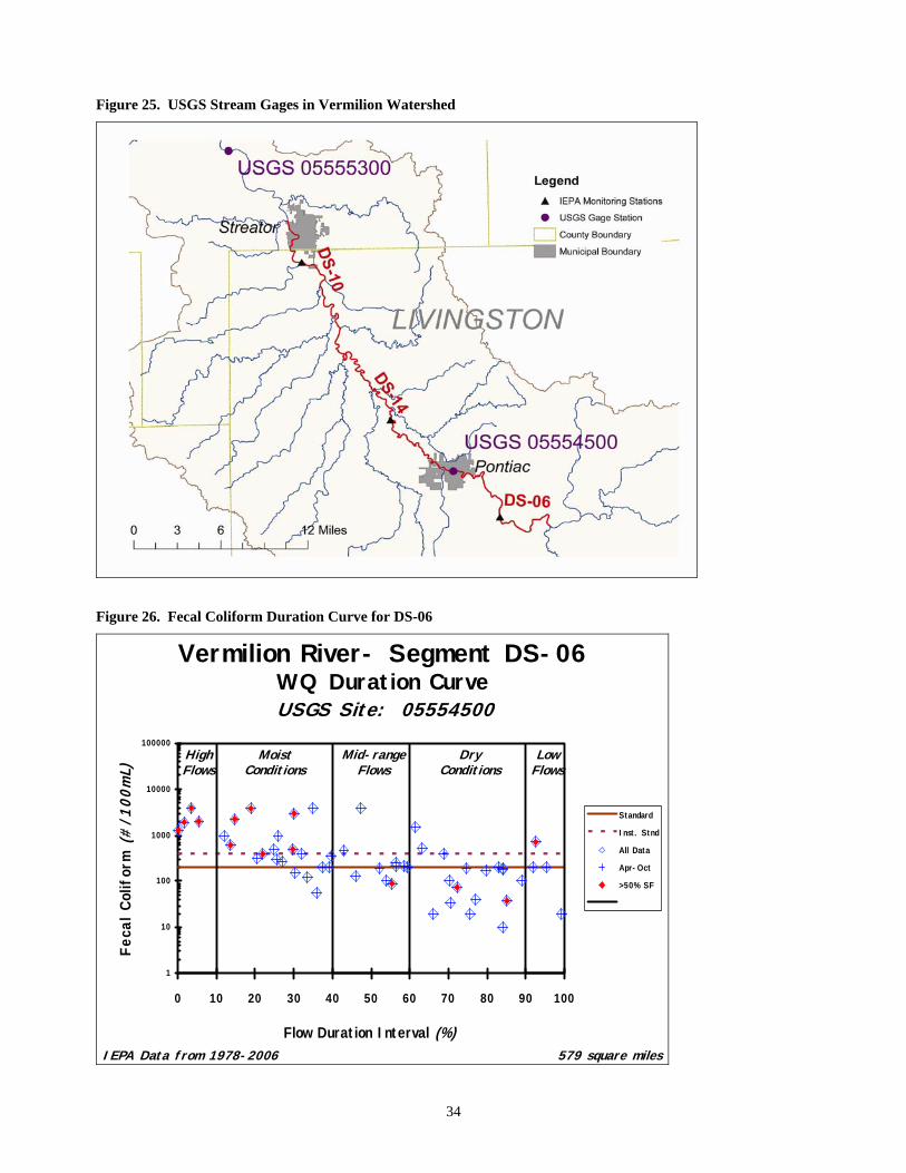
6. TMDL Development Illinois EPA is using the Duration Curve Method to develop pathogen and nitrate TMDLs. Appendix B contains Bruce Cleland’s 2003 paper entitled “TMDL Development from the “Bottom-up”- Part III: Duration Curves and Wet-weather Assessments” for more information on the duration curve method. Water quality duration curves provide a display of the water quality criterion exceedences and the flow conditions associated with their exceedences. Flows are ranked from extremely low flows, which are exceeded nearly 100 percent of the time, to extremely high flows, which are rarely exceeded. By displaying instantaneous loads calculated from ambient water quality data and the daily average flow on the date of the sample, a pattern develops, which describes the characteristics of the impairment. The pattern of impairment can be examined to see if it occurs across all flow conditions, corresponds strictly to high flow events, or conversely, only to low flow conditions (Cleland 2003). Fecal coliform loads are shown as blue diamonds on the load duration analysis and storm driven data are the red diamonds. The duration curve analysis method allows us to consider how stream flow conditions relate to a variety of pollutant loadings and their sources. Exceedences observed in low flow conditions usually indicate point source influences while high flow exceedences indicate non-point source influences and stormwater. 6.1 Water Quality Duration Curve The first step in developing a water quality duration curve is to get streamflow to tie to the water quality data from the monitoring stations. USGS stream gauges located in the watershed provided the flow data for this analysis. Data was downloaded from the USGS website. Flow data used for duration curves of Vermilion River stations DS-06 and DS-14 are from USGS gauge station 05554500 in Pontiac, Illinois. Flow data for Vermilion River station DS-10 are from USGS station 05555300 downstream of Streator. Refer to Figure 25 for station locations. The percentage of days exceeded is multiplied by the target established as a goal in this TMDL (200cfu/100mL for fecal coliform and 10 mg/L for nitrate) and a conversion factor, for the maximum allowable load associated with each flow (target load). The target load based on the standard and the observed data are then plotted on the curve. Values above the target load exceed the standard.
34
Figure 25. USGS Stream Gages in Vermilion Watershed
Figure 26. Fecal Coliform Duration Curve for DS-06
1
10
100
1000
10000
100000
0 10 20 30 40 50 60 70 80 90 100
Flow Duration Interval (%)
Feca
l Col
ifor
m (
#/1
00m
L)
Standard
Inst. Stnd
All Data
Apr-Oct
>50% SF
Vermilion River- Segment DS-06WQ Duration Curve USGS Site: 05554500
DryConditions
LowFlows
HighFlows
Mid-rangeFlows
MoistConditions
579 square milesIEPA Data from 1978-2006

35
Figure 27. Nitrate Duration Curve for DS-06
0
2
4
6
8
10
12
14
16
18
20
0 10 20 30 40 50 60 70 80 90 100
Flow Duration Interval (%)
Nitra
te (mg/
L)
Target
All Data
Apr-Oct
>50% SF
Vermilion River- Segment DS-06WQ Duration Curve
Site: 05554500
579 square milesIEPA Data from 1978-2006
DryConditions
LowFlows
HighFlows
Mid-rangeFlows
MoistConditions
Figure 28. Nitrate Duration Curve for DS-10
0
2
4
6
8
10
12
14
16
18
20
0 10 20 30 40 50 60 70 80 90 100
Flow Duration Interval (%)
Nitra
te (
mg/
L)
Target
All Data
Mar-July
>50% SF
Vermilion River- Segment DS-10WQ Duration Curve USGS Site: 5555300
1251 square milesIEPA Data 1990-2007
DryConditions
LowFlows
HighFlows
Mid-rangeFlows
MoistConditions

36
Figure 29. Nitrate Duration Curves for DS-14
0
2
4
6
8
10
12
14
16
18
20
0 10 20 30 40 50 60 70 80 90 100
Flow Duration Interval (%)
Nitra
te (
mg/
L)
Target
All Data
Mar-July
>50% SF
Vermilion River- Segment DS-14WQ Duration Curve USGS Site: 05554500
579 square milesIEPA Data 1990-2007
DryConditions
LowFlows
HighFlows
Mid-rangeFlows
MoistConditions
6.2 TMDL
Allocations A TMDL is the sum of wasteload allocations (point sources) and load allocations (Nonpoint sources) and natural background such that the capacity of the waterbodies to assimilate pollutant loading is not exceeded. A TMDL must also be developed with seasonal variations and a margin of safety that addressed uncertainty in the analysis. This TMDL will determine the maximum pollutant load the waterbodies can receive to fully support the designated use(s). Current loads are determined and if they exceed the allowable a load reduction will be given. The wasteload allocations include both permitted point sources and septic system failure estimates from systems directly discharging to waters. The total daily streamload uses the fecal coliform bacteria geometric mean for the last ten years of data for each specific station and average stream flow. Geometric means were looked at for each flow duration interval (see Table 21). The load allocation (LA) is the total daily streamload minus the waste load allocation (WLA).

37
Table 21. TMDL Load and Wasteload Allocations
Segments Flows Pollutant Actual Load (lbs/day)
WasteLoad (lb/day)
Load (lb/day)
Loading Capacity (lb/day)
Required Reduction
WasteLoad (lb/day)
Target Load (lb/day)
DS-06 High Nitrate 255953 459 255494 232684 9% 459 232225 DS-06 Moist Nitrate 31748 459 31289 26457 17% 459 25998 DS-06 Mid-Range Nitrate 5942 184 5759 7428 0% 184 7244 DS-06 Dry Nitrate 159 184 0 1586 0% 184 1402 DS-06 Low Nitrate 0 184 0 167 0% 184 0 DS-10 High Nitrate 317909 3539 314370 219247 31% 3539 215708
DS-10 Moist Nitrate 63936 3539 60397 50743 21% 3539 47204
DS-10 Mid-Range Nitrate 22350 1277 21073 21699 3% 1277 20422
DS-10 Dry Nitrate 1138 1277 0 3672 0% 1277 2395
DS-10 Low Nitrate 1 1277 0 584 0% 1277 0
DS-14 High Nitrate 162960 1736 161224 115574 29% 1736 113838 DS-14 Moist Nitrate 34772 1736 33036 31047 11% 1736 29311 DS-14 Mid-Range Nitrate 12787 709 12078 13320 0% 709 12611 DS-14 Dry Nitrate 1136 709 426 2103 0% 709 1394 DS-14 Low Nitrate 0 709 0 40 0% 709 0 DS-06 High Fecal Coliform* 3.29E+14 9.28E+10 3.29E+14 2.93E+13 91% 2.32E+10 2.92E+13
DS-06 Moist Fecal Coliform* 4.61E+12 9.28E+10 4.52E+12 2.20E+12 52% 2.32E+10 2.19E+12
DS-06 Mid-Range Fecal Coliform* 1.03E+12 6.06E+10 9.74E+11 7.42E+11 28% 9.24E+09 7.33E+11
DS-06 Dry Fecal Coliform* 8.18E+10 6.06E+10 2.12E+10 1.74E+11 0% 9.24E+09 1.65E+11
DS-06 Low Fecal Coliform* 4.33E+10 6.06E+10 -1.73E+10 2.27E+10 48% 9.24E+09 1.35E+10
* Load units for fecal coliform are cfu/100ml/day WLA for nitrate is based on the facilities designed average flow (DAF)/ designed maximum flow (DMF) and an average nitrate level of 18 mg/L in effluent for facilities with sewage treatment. DMFs are used for high and moist flow interval allocations and the DAF is used for mid-range to low flows. Nitrates may vary in concentration from 0 to 20 mg/L as N in wastewater effluents, but the typical range found in treated effluent is from 15 to 20 mg/L as N (Tchobanoglous et al 2003). All WLAs are less than one percent of the total load for each impaired stream segment for high to moist conditions when exceedences are problematic. Point sources are not considered a significant source of nitrate in the watershed and allocations will be based on the estimated nitrate value of 18mg/L. Allocation values can be updated if the current facility has nitrate data available. Point source loads for fecal coliform are based on the DAF/DMF and 200 cfu/100 ml for geometric mean and 400 cfu/100ml for instantaneous maximum for exempt facilities. DMFs are used for high and moist flow interval allocations and the DAF are used for mid-range to low flows. For exemption calculations, those segments are determined to meet this target at the end of the segment. Exempt facilities will be reevaluated in their permit renewal process and more information is available in the implementation plan. There was one facility (Stelle Community Association) that does not have an exemption and an average from their effluent data was used in the wasteload calculation. This facility is not meeting its effluent limit and more information is available in the implementation plan. The target WLA for fecal coliform is based on the designed average flow and a fecal coliform count of 200 cfu/100 ml. No CSO allocation is presented in the TMDL. Fairbury STP is a minor facility that discharges less than 400 cfu/100ml as the maximum and average loads at overflow events for their treated CSO. Fairbury does have untreated CSO discharges, but not enough information is available to determine allocations. The City is planning to build above and underground storage for any CSO discharge. The Long Term Control Plan (LTCP) for Fairbury STP is discussed in the implementation plan. There are no MS4 areas in the watershed therefore there are no MS4

38
allocations included in the WLA. There are no allowable septic loads because it is illegal to discharge untreated waste into streams, so septic loads have a zero allowable load. The allowable load is the total allowable streamload minus the allowable wasteload. Appendix A contains all specific calculations for each stream segment. Table 21 contains all the allocations for each segment. Table 22 contains all the point source loads used in the allocation calculations for each segment. Table 22. Point Source Wasteloads by Segment
NPDES ID Facility Name DAF (MGD)
DMF (MGD
Fecal Load (200)
cfu/100ml/MGD) DAF/DMF
Fecal Load (400)
cfu/100ml/MGD) DAF/DMF
Nitrate Load (18mg/L)
mg/L/MGD DAF/DMF
Nitrate Load (18mg/L) lbs/day
DAF/DMF
ILG580091 Chatsworth STP
0.18 0.46 36 / 92 72 / 184 3.2 / 8.3 27 / 69
IL0037001 Greenbriar Health Care
0.01 0.032 2 / 6.4 4 / 12.8 0.2 / 0.6 1.5 / 4.8
IL0021601 Fairbury STP 0.66 1.65 132 / 330 264 / 660 11.9 / 30 99 / 248
IL0028819 Forrest STP 0.35 0.88 70 / 176 140 / 352 6.3 / 15.8 53 / 132
IL0026697 Stelle Community Assn STP
0.02 0.04 4 / 8 4 / 16 0.4 / 0.7 3 / 6
Total Load for DS-06
244 / 612 488 / 1225 22 / 55 183 / 460
IL0030457 Pontiac STP 3.5 8.5 63 / 153 525 / 1276
Total Load for DS-14
63 / 153 525 / 1276
ILG582009 Chenoa STP 0.26 0.658 4.68 / 11.844 39 / 99
ILG580057 Flanagan STP 0.13 0.32 2.34 / 5.76 20 / 48
ILG551069 IL DOT-I-55 Livingston Co
0.02 0.047 0.36 / 0.827 3 / 7
ILG551020 Meadows Mennonite Ret.
0.05 0.113 0.9 / 0.2025 8 / 17
ILG551038 Salem Childrens
Home
0.01 0.03 0.18 / 0.54 2 / 5
IL0022004 Streator STP 3.3 10.8 59.4 / 194.4 495 / 1621
IL0048828 Woodland School
0.01 0.03 0.18 / 0.54 2 / 5
Total Load for DS-10
68 / 216 567 / 1801
*DMF (daily maximum flow) used for wasteload allocations for high flow interval only The geometric mean for each interval can show which flow periods need reductions (see Table 23). This can be used to look at implementation/ management opportunities (see Table 24). Most geometric mean exceedences for nitrate occur during high or moist flow intervals. Table 23. Geometric Means and for Flow Intervals
Duration Curve Zone
Geometric Mean High Moist Mid Dry Low
Vermilion R. DS-06 Nitrate (mg/L) 11 12 8 1 0Vermilion R. DS-10 Nitrate (mg/L) 14 13 10 3 0Vermilion R. DS-14 Nitrate (mg/L) 14 11 10 5 0Vermilion R. DS-06 Fecal Coliform(cfu/100ml) 2252 420 279 94 381

39
Table 24 . Management Practices
High Moist Mid-Range Dry Low
Streambank Stabilization X CSO Long Term Plan X X Managing Manure Application X X Nutrient Management Plans X X X Erosion Control X X X Pasture / Grazing Management X X Managing Barnyards X X Riparian Buffers X X X Managing Private Systems X X X Replacing Failed Systems X X X Point Source Controls X X Remove Illicit Discharges X X
Margin of Safety Section 303(d)(1)C of the Clean Water Act and USEPA’s regulations at 40 CFR 130.7 require that “TMDLs shall be established at levels necessary to attain and maintain the applicable narrative and numerical water quality standards with seasonal variations and a margin of safety which takes into account any lack of knowledge concerning the relationship between effluent limitations and water quality.” The margin of safety can either be implicitly incorporated into conservative assumptions used to develop the TMDL or added as a separate explicit component of the TMDL (USEPA, 1991). Most TMDLs use models or spreadsheet calculations that use assumptions as part of the load calculations. These assumptions are sometimes broad numbers that are not specific for the watershed. The load duration curve does not use assumptions and is based on specific flow and water quality data for the streams in the watershed. Therefore, no margin of safety is needed for this TMDL.
Seasonality Because this is a concentration-based TMDL, the fecal coliform and nitrate standard will be met regardless of flow conditions in the applicable season. Data from all seasons for chemical samples, flow and NPDES monitoring data were used.
Critical Conditions Each stream segment may have a different critical condition. The load duration curve shows the flow period(s) where there are standard exceedences, which can tie into the sources at those flow conditions. Critical conditions for each segment will be discussed in the implementation plan.

40
7. Public Participation The public participation process for TMDLs is addressed through the use of a series of public meetings and reports made available to the public. The purpose of the public meetings is to provide information on the TMDL process and to take comments on the draft reports. Illinois EPA holds a minimum of two public meetings; one at the beginning of the TMDL process and one towards the end. For the first public meeting, Illinois EPA sent out public notices to newspapers in the watershed; the Tonica News, Pontiac Daily Leader, Fairbury Blade, Chenoa Town Crier and the Ottawa Times. 130 public notices were also sent out to organizations/individuals such as the Farm Bureau, Soil and Water Conservation Districts, Extension offices, state and federal elected officials, county/ city /village officials and NPDES facilities. The Report is available online at the TMDL website, www.epa.state.il.us/water/tmdl, and hard copies were mailed to Streator City Hall, Minonk City Hall, Pontiac City Hall and Piper City Village Hall. There were 25 people at the Stage 1 meeting on June 13, 2007 at the University of Illinois Extension Building in Pontiac, IL. The second public meeting is planned for August 20, 2009 at the Extension Building in Pontiac. This will discuss the Stage 3 and Implementation Plan. There will be a 13 day public comment period in which the Illinois EPA will respond to those comments in a Responsiveness Summary that will be included in the final TMDL Report.
41
8. References Cleland, Bruce. 2003. TMDL Development From the “Bottom Up” Part III: Duration Curves and Wet-
Weather Assessments. American’s Clean Water Foundation. Washington, DC. Illinois Department of Agriculture. 2004. 2004 Illinois Soil Conservation Transect Survey Summary. State
of Illinois. Illinois Environmental Protection Agency. 1998. Clean Water Act Section 303(d) List: Illinois’ Submittal
for 1998. IEPA/BOW/97-023. Bureau of Water, Division of Water Pollution Control. Springfield, Illinois.
Illinois EPA. 1999. Livestock and Wildlife Densities in Illinois. IEPA. Springfield, Illinois Illinois EPA. 2002. Illinois 2002 Section 303(d) List. IEPA/BOW/03-016. Bureau of Water, Watershed
Management Section. Springfield, Illinois Illinois EPA. 2004. Illinois 2004 Section 303(d) List. IEPA/BOW/04-005. Bureau of Water, Watershed
Management Section. Springfield, Illinois Illinois EPA. 2004. Illinois Water Quality Report 2004. IEPA/BOW/04-006. Bureau of Water, Division of
Water Pollution Control. Springfield, Illinois. Minnesota Pollution Control Agency. 2002. Regional TMDL Evaluation of Fecal Coliform Bacteria
Impairment in the Lower Mississippi River Basin in Minnesota. Regional Environmental Management Division. Minnesota.
National Small Flow Clearinghouse. 2001. A Summary of the Status of Onsite Wastewater Treatment
Systems in the United States during 1998. West Virginia University. Morgantown, West Virginia. Tchobanoglous, G., Burton, F.L., and Stensel, H.D. 2003. Wastewater Engineering (Treatment
Disposal Reuse) / Metcalf & Eddy, Inc., 4th Edition. McGraw-Hill Book Company U.S. EPA 2001. Protocol for Developing Pathogen TMDLs. EPA 841-R-00-002. U.S. EPA. Washington
D.C. United States Environmental Protection Agency. 1986. Ambient Water Quality Criteria for Bacteria- 1986.
EPA-A4401/5-84-002. U.S. EPA. Washington, DC.

42

Appendix A
Load Calculations for Individual Water Segments


Loads Vermilion River DS-06 Nitrate
Total Load- Geo Mean (mg/L) Average Flow MGD gal/MGD L/gal lb/mg lb/d1 11 2788 1,000,000 3.785 0.000002205 2.56E+052 12 317 1,000,000 3.785 0.000002205 3.17E+04
8 89 1,000,000 3.785 0.000002205 5.94E+031 19 1,000,000 3.785 0.000002205 1.59E+020 2 1,000,000 3.785 0.000002205 0.00E+00
Wasteload- NPDES Discharge (mg/L/MGD)
gal/MGD L/gal lb/mg lb/d NPDES discharge high
flow
Permitted WL at high flows
22 1,000,000 3.785 2.205E-06 1.84E+02 55 459.025875Septic Wasteload - Households Nitrate (mg/L) discharge
(gal/person/d) people/
house ml/gal L/mL g/mg lb/mg lb/d
5 1.60E+01 70 2.5 3785.2 0.001 0.001 0.000002205 1.17E-04Total Wasteload- MS4 WL Septic lb/d
0.00E+00 1.84E+02 1.17E-04 1.84E+02Load- Total Annual Load - Wasteload = cfu/d
2.56E+05 4.59E+02 2.55E+053.17E+04 4.59E+02 3.13E+045.94E+03 1.84E+02 5.76E+031.59E+02 1.84E+02 -2.50E+010.00E+00 1.84E+02 -1.84E+02
Allowable Load
Permitted Wasteload- NPDES Discharge (ml/L/mgd)
gal/MGD L/gal lb/mg lb/d NPDES discharge high
flow
Permitted WL at high flows
22 1,000,000 3.785 2.205E-06 1.84E+02 55 4.59E+02Loading Capacity- Target (mg/L) Annual Seasonal Flow
(MGD) gal/MGD L/gal lb/mg lb/d
10 2788 1 000 000 3 785 0 000002205 2 33E+0510 2788 1,000,000 3.785 0.000002205 2.33E+0510 317 1,000,000 3.785 0.000002205 2.65E+0410 89 1,000,000 3.785 0.000002205 7.43E+0310 19 1,000,000 3.785 0.000002205 1.59E+0310 2 1,000,000 3.785 0.000002205 1.67E+02
Load Allowable- Total Allowable Load Allowable Wasteload lb/d2.33E+05 4.59E+02 2.32E+052.65E+04 4.59E+02 2.60E+047.43E+03 1.84E+02 7.24E+031.59E+03 1.84E+02 1.40E+031.67E+02 1.84E+02 -1.67E+01
Actual Load (lbs/day) WasteLoad (lb/day) Load (lb/day) Loading Capacity
Required Reduction WasteLoad (lb/day) Target Load (lb/day)
High Flow 255953 459 255494 232684 9% 459 232225Moist Conditions 31748 459 31289 26457 17% 459 25998
Mid-Range Flows 5942 184 5759 7428 0% 184 7244Dry Conditions 159 184 0 1586 0% 184 1402
Low Flows 0 184 0 167 0% 184 0

Loads Vermilion River DS-06 Fecal
Total Load- Geo Mean (cfu/ml) Average Flow MGD gal/MGD L/gal ml/L cfu/d1 22.52 3865 1,000,000 3.785 1000 3.29E+142 4.2 290 1,000,000 3.785 1000 4.61E+12
2.79 98 1,000,000 3.785 1000 1.03E+120.94 23 1,000,000 3.785 1000 8.18E+103.81 3 1,000,000 3.785 1000 4.33E+10
Wasteload- NPDES Discharge (cfu/ml/MGD)
gal/MGD L/gal ml/L cfu/d NPDES discharge high flow
7.26 1,000,000 3.785 1000 2.75E+10 15.76 5.97E+10Septic Wasteload - Households Fecal (cfu/ml) discharge
(gal/person/d) people/
house ml/gal cfu/d
5 1.00E+04 70 2.5 3785.2 3.31E+10Wasteload- MS4 WL Septic lb/d High Flows
0.00E+00 2.75E+10 3.31E+10 6.06E+10 9.28E+10Load- Total Annual Load - Wasteload = cfu/d
3.29E+14 9.28E+10 3.29E+144.61E+12 9.28E+10 4.52E+121.03E+12 6.06E+10 9.74E+118.18E+10 6.06E+10 2.12E+104.33E+10 6.06E+10 -1.73E+10
Allowable Load
Permitted Wasteload- NPDES Discharge (ml/L/mgd)
gal/MGD L/gal ml/L cfu/d NPDES discharge high flow
Permitted WL at high flows
2.44 1,000,000 3.785 1000 9.24E+09 6.12 2.32E+10Loading Capacity- Target (mg/L) Annual Seasonal Flow
(MGD) gal/MGD L/gal ml/L lb/d
2 3865 1,000,000 3.785 1000 2.93E+132 290 1,000,000 3.785 1000 2.20E+122 98 1,000,000 3.785 1000 7.42E+112 23 1,000,000 3.785 1000 1.74E+112 3 1,000,000 3.785 1000 2.27E+10
Load Allowable- Total Allowable Load Allowable Wasteload lb/d2.93E+13 2.32E+10 2.92E+132.20E+12 9.24E+09 2.19E+127.42E+11 9.24E+09 7.33E+111.74E+11 9.24E+09 1.65E+112.27E+10 9.24E+09 1.35E+10
Actual Load (cfu/day) WasteLoad (cfu/day) Load (cfu/day) Loading Capacity (cfu/day)
Required Reduction
Allowable WasteLoad (cfu/day)
Target Load (cfu/day)
High Flow 3.3E+14 9.28E+10 3.3E+14 2.9E+13 91% 2.32E+10 2.9E+13Moist Conditions 4.6E+12 9.3E+10 4.5E+12 2.2E+12 52% 2.32E+10 2.2E+12
Mid-Range Flows 1.0E+12 6.1E+10 9.7E+11 7.4E+11 28% 9.2E+09 7.3E+11Dry Conditions 8.2E+10 6.1E+10 2.1E+10 1.7E+11 0% 9.2E+09 1.6E+11
Low Flows 4.3E+10 6.1E+10 -1.7E+10 2.3E+10 48% 9.2E+09 1.3E+10

Loads Vermilion River DS-14 NitrateTotal Load- Geo Mean (mg/L) Average Flow MGD gal/MGD L/gal lb/mg lb/d1 14.1 1384.8 1,000,000 3.785 0.000002205 1.63E+052 11.2 372 1,000,000 3.785 0.000002205 3.48E+04
9.6 159.6 1,000,000 3.785 0.000002205 1.28E+045 25.2 1,000,000 3.785 0.000002205 1.14E+030 0.48 1,000,000 3.785 0.000002205 0.00E+00
Wasteload- NPDES Discharge (mg/L/MGD)
gal/MGD L/gal lb/mg lb/d NPDES discharge high
flow
Permitted WL at high flows
85 1,000,000 3.785 2.205E-06 7.09E+02 208 1735.9524Septic Wasteload - Households Nitrate (mg/L) discharge
(gal/person/d) people/
house ml/gal L/mL g/mg lb/mg lb/d
7 1.60E+01 70 2.5 3785.2 0.001 0.001 0.000002205 1.64E-04Wasteload- MS4 WL Septic lb/d
0.00E+00 7.09E+02 1.64E-04 7.09E+02Load- Total Annual Load - Wasteload = cfu/d
1.63E+05 1.74E+03 1.61E+053.48E+04 1.74E+03 3.30E+041.28E+04 7.09E+02 1.21E+041.14E+03 7.09E+02 4.26E+020.00E+00 7.09E+02 -7.09E+02
Allowable Load
Permitted Wasteload- NPDES Discharge (ml/L/mgd)
gal/MGD L/gal lb/mg lb/d NPDES discharge high
flow
Permitted WL at high flows
85 1,000,000 3.785 2.205E-06 7.09E+02 208 1735.9524Loading Capacity- Target (mg/L) Annual Seasonal Flow
(MGD) gal/MGD L/gal lb/mg lb/d
10 1384.8 1,000,000 3.785 0.000002205 1.16E+0510 372 1,000,000 3.785 0.000002205 3.10E+0410 159.6 1,000,000 3.785 0.000002205 1.33E+0410 25.2 1,000,000 3.785 0.000002205 2.10E+0310 0.48 1,000,000 3.785 0.000002205 4.01E+01
Load Allowable- Total Allowable Load Allowable Wasteload lb/d1.16E+05 1.74E+03 1.14E+053.10E+04 1.74E+03 2.93E+041.33E+04 7.09E+02 1.26E+042.10E+03 7.09E+02 1.39E+034.01E+01 7.09E+02 -6.69E+02
Actual Loads (lbs/day) WasteLoad (lb/day) Load (lb/day) Loading Capacity
Required Reduction
Wasteload (lb/day) Target Load (lb/day)
High Flow 162960 1736 161224 115574 29% 1736 113838Moist Conditions 34772 1736 33036 31047 11% 1736 29311
Mid-Range Flows 12787 709 12078 13320 0% 709 12611Dry Conditions 1136 709 426 2103 0% 709 1394
Low Flows 0 709 0 40 0% 709 0
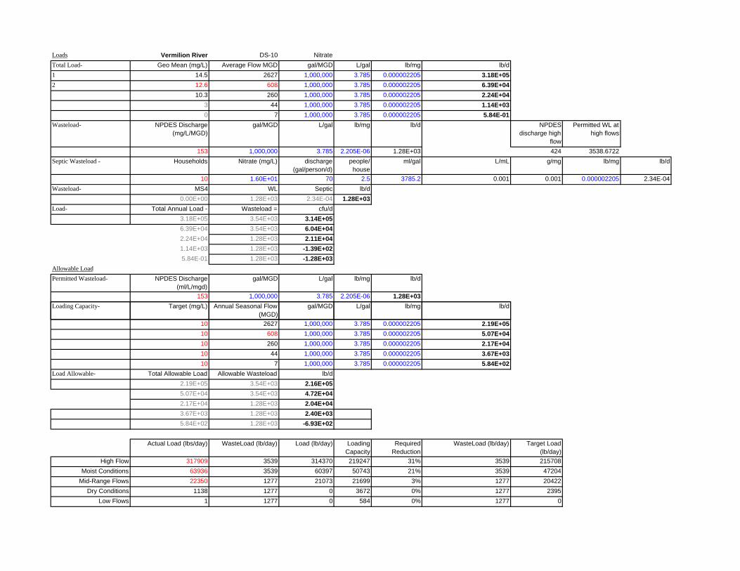
Loads Vermilion River DS-10 NitrateTotal Load- Geo Mean (mg/L) Average Flow MGD gal/MGD L/gal lb/mg lb/d1 14.5 2627 1,000,000 3.785 0.000002205 3.18E+052 12.6 608 1,000,000 3.785 0.000002205 6.39E+04
10.3 260 1,000,000 3.785 0.000002205 2.24E+043 44 1,000,000 3.785 0.000002205 1.14E+030 7 1,000,000 3.785 0.000002205 5.84E-01
Wasteload- NPDES Discharge (mg/L/MGD)
gal/MGD L/gal lb/mg lb/d NPDES discharge high
flow
Permitted WL at high flows
153 1,000,000 3.785 2.205E-06 1.28E+03 424 3538.6722Septic Wasteload - Households Nitrate (mg/L) discharge
(gal/person/d) people/
house ml/gal L/mL g/mg lb/mg lb/d
10 1.60E+01 70 2.5 3785.2 0.001 0.001 0.000002205 2.34E-04Wasteload- MS4 WL Septic lb/d
0.00E+00 1.28E+03 2.34E-04 1.28E+03Load- Total Annual Load - Wasteload = cfu/d
3.18E+05 3.54E+03 3.14E+056.39E+04 3.54E+03 6.04E+042.24E+04 1.28E+03 2.11E+041.14E+03 1.28E+03 -1.39E+025.84E-01 1.28E+03 -1.28E+03
Allowable LoadPermitted Wasteload- NPDES Discharge
(ml/L/mgd) gal/MGD L/gal lb/mg lb/d
153 1,000,000 3.785 2.205E-06 1.28E+03Loading Capacity- Target (mg/L) Annual Seasonal Flow
(MGD) gal/MGD L/gal lb/mg lb/d
( )10 2627 1,000,000 3.785 0.000002205 2.19E+0510 608 1,000,000 3.785 0.000002205 5.07E+0410 260 1,000,000 3.785 0.000002205 2.17E+0410 44 1,000,000 3.785 0.000002205 3.67E+0310 7 1,000,000 3.785 0.000002205 5.84E+02
Load Allowable- Total Allowable Load Allowable Wasteload lb/d2.19E+05 3.54E+03 2.16E+055.07E+04 3.54E+03 4.72E+042.17E+04 1.28E+03 2.04E+043.67E+03 1.28E+03 2.40E+035.84E+02 1.28E+03 -6.93E+02
Actual Load (lbs/day) WasteLoad (lb/day) Load (lb/day) Loading Capacity
Required Reduction
WasteLoad (lb/day) Target Load (lb/day)
High Flow 317909 3539 314370 219247 31% 3539 215708Moist Conditions 63936 3539 60397 50743 21% 3539 47204
Mid-Range Flows 22350 1277 21073 21699 3% 1277 20422Dry Conditions 1138 1277 0 3672 0% 1277 2395
Low Flows 1 1277 0 584 0% 1277 0

Appendix B
TMDL Development from Bottom-up
By Bruce Cleland


TMDL Development from the “Bottom Up” -- Part III: Duration Curves and Wet-Weather Assessments
1 September 15, 2003
TMDL DEVELOPMENT FROM THE “BOTTOM UP” – PART III: DURATION CURVES AND WET-WEATHER ASSESSMENTS
Bruce Cleland
America’s Clean Water Foundation 750 First Street N.E. – Suite #1030
Washington, DC 20002 E-Mail: [email protected]
ABSTRACT With the large number of TMDLs to be completed, limited resources, and the complex, inter-related nature of water programs – the “two Ps”: practical approaches and partnerships – are critical to success. Dependable tools are needed to promote effective communication between TMDL developers and implementers, so that actions will lead to measurable water quality improvements. A “bottom up” approach is one way to establish a meaningful, value-added framework linking water quality concerns to proposed solutions. A “bottom up” approach capitalizes on the networks of programs and authorities across jurisdictional lines. Kansas has been utilizing load duration curves for the past several years as a key part of its TMDL development process. The increased use of duration curves supports the “bottom up” approach by offering an opportunity for enhanced targeting, both in TMDL development and in water quality restoration efforts. Duration curves can also add value to the TMDL process by expanding the characterization of water quality concerns, linking concerns to key watershed processes, prioritizing source assessment efforts, and identifying potential solutions. Flow duration curve analysis identifies intervals, which can be used as a general indicator of hydrologic condition (i.e. wet versus dry and to what degree). This indicator, when combined with other basic elements of watershed planning, can help point problem solution discussions towards relevant watershed processes, important contributing areas, and key delivery mechanisms. Duration curves are not a substitute for field reconnaissance work. Grounded, fact- finding is needed to examine what is actually going on in the watershed. Duration curves do, however, offer a framework that can help refine water quality assessment s. Refined analyses using duration curves can be important considerations when identifying those controls that might be most appropriate and under what conditions. This paper uses several examples to illustrate opportunities where duration curves can strengthen watershed assessments and enhance the TMDL development process. KEYWORDS Flow duration curves, watershed analysis, BMP targeting, adaptive management

TMDL Development from the “Bottom Up” -- Part III: Duration Curves and Wet-Weather Assessments
2 September 15, 2003
INTRODUCTION A strength of the total maximum daily load (TMDL) program is its ability to support development of information-based, water quality management strategies. If done properly, a TMDL “can inform, empower, and energize citizens, local communities, and States to improve water quality at the local, watershed level. The basic information derived from a sound TMDL could liberate the creative energies of those most likely to benefit from reduced pollutant loadings to their own waters” (Tracy Mehan, November 2001). Dependable tools are needed to promote effective communication between TMDL developers and implementers, so that actions will lead to measurable water quality improvements. With the large number of TMDLs to be completed, limited resources by all involved with watershed management, and the complex, inter-related nature of water programs – the “two Ps”: practical approaches and partnerships – are critical to success. Public involvement is fundamental to successful TMDL development and implementation. Key stakeholders in the watershed must be engaged in order to achieve meaningful results. Kansas has been utilizing duration curves as a key part of its TMDL development process. The increased use of duration curves offers an opportunity for enhanced targeting, both in TMDL development and in water quality restoration efforts. Duration curves can also add value to the TMDL process by expanding the characterization of water quality concerns, linking concerns to key watershed processes, prioritizing source assessment efforts, and identifying potential solutions. Duration curve analysis identifies intervals, which can be used as a general indicator of hydrologic condition (i.e. wet versus dry and to what degree). This indicator, when combined with other basic elements of watershed planning, can help point problem solution discussions towards relevant watershed processes, important contributing areas, and key delivery mechanisms. These are all major considerations when identifying those controls that might be most appropriate and under what conditions. Duration curves also give a context for evaluating both monitoring data and modeling information. Water quality monitoring data used in a duration curve framework can support watershed planning by:
* Providing a better description of water quality concerns * Improving the basic understanding of key watershed processes * Focusing solution development
This offers another way to look at identifying data needs where adaptive management is being considered or utilized.

TMDL Development from the “Bottom Up” -- Part III: Duration Curves and Wet-Weather Assessments
3 September 15, 2003
“BOTTOM UP” APPROACHES An important key to the success of the TMDL program, in terms of engaging the public, is building linkages to other programs, such as nonpoint source (NPS) management. Many successful efforts to develop TMDLs, for example, have involved the §319 program as a way to utilize local groups in data collection, ana lysis, and implementation. Watershed analysis has been used to build a “bottom up” approach as one way to establish a meaningful, value-added framework linking water quality concerns to proposed solutions. TMDL development using a “bottom up” approach considers the interaction between watershed processes, disturbance activities, and available methods to reduce pollutant loadings, specifically Best Management Practices (BMPs). A “bottom up” approach capitalizes on the networks of programs and authorities across jurisdictional lines. Information on management measures related to both source control and delivery reduction methods can be incorporated into the allocation part of TMDL development. Problem Solving Framework The “two Ps” – practical approaches and partnerships – are critical to successful watershed planning and implementation. On the practical side, a “bottom up” approach must overcome the challenge of translating detailed technical concepts and information into “plain English”. On the partnership side, key stakeholders must be engaged in the process, so that meaningful results with measurable improvements are achieved. A problem solving framework, constructed around a set of fundamental questions, can help focus development of practical approaches and encourage participation among key partners. A basic set of questions using a “bottom up” approach to address water quality problems often includes:
* WHY the concern? * WHAT reductions are needed? * WHERE are the sources? * WHO needs to be involved? * WHEN will actions occur?
These simple, practical questions can be easily used to keep assessment efforts connected with implementation activities. Methods to communicate technical information are an important part of the problem solving process.

TMDL Development from the “Bottom Up” -- Part III: Duration Curves and Wet-Weather Assessments
4 September 15, 2003
Communicating Technical Information An advantage of the duration curve framework is its ability, as a simple communication tool, to help answer some of the basic questions. This benefit includes not only TMDL development, but also extends to water quality assessment (enhanced description of concerns) and implementation planning (focus on meaningful solutions through understanding key watershed processes that deliver pollutants). The following example briefly illustrates the “added value” that duration curves can provide. Figure 1 illustrates a load duration curve developed for a watershed where sediment is causing impairments to resident trout populations. This load duration curve was developed to look at several issues. The first was to better characterize conditions surrounding water quality concerns. The second involved the relative importance of point sources in light of the timing of sediment load concerns. The third focused on the type of management practices (BMPs) that would be most effective.
Figure 1. Example Load Duration Curve

TMDL Development from the “Bottom Up” -- Part III: Duration Curves and Wet-Weather Assessments
5 September 15, 2003
As indicated in Figure 1, duration curves can be a very useful tool to characterize water quality concerns and to describe patterns associated with the impairment. The use of duration curve zones (e.g. high flows, moist conditions, etc.) provides a method for communicating technical information in a way that easily conveys conditions associated with problems. The results of the quick duration curve analysis shown in Figure 1 indicate point sources, which generally tend to be most significant during low flows, do not appear to be major contributors. Practices that target delivery reduction (riparian buffers) and source control (contour farming, conservation tillage) under mid-range flows and moist conditions appear to offer the greatest benefit. The concept of grouping water quality data based on flow conditions is not new. A duration curve framework simply provides a way to organize the information. Ideas behind the duration curve approach can also be extended to the way in which a TMDL is presented, as shown in Table 1. This situation, different from Figure 1, depicts a fecal coliform TMDL for a fairly complex watershed affected by point sources, combined sewer overflows (CSOs), and the full array of land uses (urban, agricultural, woodland).
Table 1. Example TMDL Using Duration Curve Framework
High Moist Mid-Range Dry Low
Reduction 92% 90% 78% 40% 0%TMDL 1.39E+14 5.09E+13 2.37E+13 1.15E+13 5.09E+12
Load Allocations 9.32E+12 2.73E+12 2.26E+13 1.05E+13 4.22E+12Wasteload Allocations 4.68E+11 4.68E+11 4.68E+11 4.68E+11 4.68E+11
CSO 1.25E+14 4.58E+13 0.00E+00 0.00E+00 0.00E+00Margin of Safety 4.11E+12 1.89E+12 6.20E+11 4.99E+11 4.06E+11
ImplementationOpportunities
Loads expressed as (cfu/day)
Long Term CSO Plan Municipal NPDESRiparian ProtectionPet Waste OrdinanceStormwater Mgt.
A common challenge faced by TMDL practitioners is explaining how the loads, which are an element of the TMDL, translate to potential actions. In addition to loads, Table 1 uses a duration curve framework to summarize reduction targets and to highlight implementation opportunities that correspond to flow conditions. As communication tools, the graphic display and table can be combined with other basic elements of watershed planning to help guide problem solving discussions in a meaningful way. Duration curves, like any other analytical tool, are not a substitute for field reconnaissance work. Good watershed assessment, which leads to effective management plans, cannot be limited to “desk-top” exercises. Grounded, fact-finding is needed to examine what is actually going on in the watershed. Duration curves can, however, highlight relevant watershed conditions, processes, and potential solutions.

TMDL Development from the “Bottom Up” -- Part III: Duration Curves and Wet-Weather Assessments
6 September 15, 2003
Engaging Stakeholders Public involvement is fundamental to successful TMDL development and implementation. Duration curves provide another way of presenting water quality data, which characterizes concerns and describes patterns associated with impairments. As a communication tool, this framework can help elevate the importance of monitoring information to stakeholders. This in turn can encourage locally driven data collection efforts (e.g. through watershed groups, conservation districts, point sources). The extended use of monitoring information and the alternative way to present TMDLs using duration curves offers an opportunity for enhanced targeting, both in field investigation efforts and implementation planning. In particular, duration curves support a “bottom up” approach by identifying targeted areas, targeted programs, targeted activities, and targeted participants. As an assessment and communication tool, duration curves can help narrow potential debates, as well as inform the public and stakeholders so they become engaged in the process. The discussion that follows provides more detail on the development of duration curves. This paper also describes ways in which duration curves may be applied to develop water quality management plans and TMDLs, with a focus on wet-weather assessments. DURATION CURVES Water resource planners have utilized stream flow data for many years to support a variety of activities ranging from development of public water supplies to fisheries management and flood control. A network of river gaging stations and the published data obtained from their operation supports these water resource management efforts (Leopold, 1994). Information on river flows across the United States is readily available from the U.S. Geological Survey. Due to the wide range of variability that can occur in stream flows, hydrologists have long been interested in knowing the percentage of days in a year when given flows occur. Development of Flow Duration Curves The percentage of time during which specified flows are equaled or exceeded may be evaluated using a flow duration curve (Leopold, 1994). Flow duration analysis looks at the cumulative frequency of historic flow data over a specified period. The duration analysis results in a curve, which relates flow values to the percent of time those values have been met or exceeded. Thus, the full range of stream flows is considered. Low flows are exceeded a majority of the time, whereas floods are exceeded infrequently. A typical curve runs from high to low along the x-axis, as illustrated in Figure 2.

TMDL Development from the “Bottom Up” -- Part III: Duration Curves and Wet-Weather Assessments
7 September 15, 2003
Figure 2. General Form of the Flow Duration Curve
The development of a flow duration curve typically uses daily average discharge rates, which are sorted from the highest value to the lowest (Figure 2). Using this convention, flow duration intervals are expressed as percentage, with zero corresponding to the highest stream discharge in the record (i.e. flood conditions) and 100 to the lowest (i.e. drought conditions). Thus, a flow duration interval of sixty associated with a stream discharge of 82 cubic feet per second (cfs) implies that sixty percent of all observed stream discharge values equal or exceed 82 cfs. Enhanced Targeting Traditional approaches towards TMDL development tend to focus on targeting a single value, which depends on a water quality criterion and design flow. The single number concept does not work well when dealing with impairments caused by NPS pollutant inputs (Stiles, 2001). One of the more important concerns regarding nonpoint sources is variability in stream flows, which often causes different source areas and loading mechanisms to dominate under different flow regimes. Because NPS pollution is often driven by runoff events, TMDL development should consider factors that ensure adequate water quality across a range of flow conditions.

TMDL Development from the “Bottom Up” -- Part III: Duration Curves and Wet-Weather Assessments
8 September 15, 2003
Duration curves offer an opportunity for enhanced targeting, both in TMDL development and in water quality restoration efforts. In particular, duration curves can add value to the TMDL process by identifying:
* targeted participants (e.g. NPDES permitees) at critical flow conditions; * targeted programs (e.g. Conservation Reserve Program); * targeted activities (e.g. conservation tillage or contour farming); and * targeted areas (e.g. bank stabilization projects).
Figure 3 represents the first of several hypothetical examples to illustrate the potential use of duration curves, both as a diagnostic indicator and as a communication tool for targeting in the TMDL process. The target curve in Figure 3 is derived using flow duration intervals that correspond to stream discharge values and numeric criteria for E. Coli. Several TMDL practitioners have described this technique (Stiles, 2001; Bonta, 2002; Sullivan, 2002; Sheely, 2002). The area circled on the right side of the duration curve represents hydrologic conditions where the target is exceeded. In this example, wastewater treatment plants exert a significant influence at low flows. Thus, duration curves support a “bottom up” approach towards TMDL development and restoration efforts by identifying targeted participants, in the case of Figure 3, point sources.
Figure 3. Duration Curve as General Indicator of Hydrologic Condition

TMDL Development from the “Bottom Up” -- Part III: Duration Curves and Wet-Weather Assessments
9 September 15, 2003
Figure 4 illustrates the added value duration curves can provide by highlighting potential contributing areas. As seen in this hypothetical example, the target is met when the hydrologic condition of the watershed is above a flow duration interval of 70 (generally low flow and dry conditions). Problems start to develop under mid-range flow and sometimes dry conditions, as indicated by the circled area. Wet-weather events can range from high flows and moist conditions due to severe thunderstorms to lower surface runoff following light rains. Watershed conditions, land use, and proximity of source areas to streams should also be considered. For this particular watershed (Figure 4), the increased load may be the result of pollutant delivery associated with rainfall and runoff from riparian areas. In more urban watersheds, runoff from impervious areas could also contribute flow and pollutants in response to light rain, exhibiting a pattern similar to Figure 4. Duration curves can be used as a diagnostic tool, which supports a “bottom up” approach towards TMDL development and water quality restoration by identifying targeted programs, namely those focused on riparian protection. In agricultural areas, such as the Willow Creek example watershed, this might include activities such as the Conservation Reserve Program (CRP) and Conservation Reserve Enhancement Program (CREP).
Figure 4. Duration Curve with Contributing Area Focus

TMDL Development from the “Bottom Up” -- Part III: Duration Curves and Wet-Weather Assessments
10 September 15, 2003
The focus on contributing areas is further illustrated with another hypothetical example, shown in Figure 5, where total suspended solids is the pollutant of concern. Here, the duration curve is expressed in terms of yield to show how distributions derived from a flow duration curve can be extended to other measures, again as a simple targeting tool. In the Chicken Run example (Figure 5), observed values only exceed the target when the hydrologic condition of the watershed is below 55 (generally higher flows). For the Chicken Run example watershed, duration curves can be used to support a “bottom up” approach towards TMDL development. Chicken Run is also an agricultural watershed. Wet-weather events expected to deliver pollutants under moist conditions are generally associated with more saturated soils. In addition to riparian areas, a larger portion of the watershed drainage area is potentially contributing runoff. In this case, consideration might be given to targeted activities such as conservation tillage, contour strips, and grassed waterways. Thus, water quality data and a duration curve framework can help guide local implementation efforts to achieve meaningful results.
Figure 5. Duration Curve with Contributing Area Focus

TMDL Development from the “Bottom Up” -- Part III: Duration Curves and Wet-Weather Assessments
11 September 15, 2003
Figure 6 illustrates another hypothetical example, where delivery mechanisms could include streambank erosion processes. Targeted areas for water quality improvement might consider bank stabilization efforts.
Figure 6. Duration Curve with Delivery Mechanism Focus
Extending Duration Curves to Wet-Weather TMDLS An advantage of the duration curve framework is its ability, as a simple communication tool, to link potential implementation efforts to the hydrologic condition of the watershed and to improve targeting of watershed restoration activities. The approach can examine relationships between source area / delivery mechanisms (e.g. point source discharges, storm-event runoff) and the corresponding watershed response, in a way that accounts for the range of different hydrologic conditions. A duration curve framework can support TMDL development intended to address wet-weather problems by:
* enhancing the characterization of water quality concerns * linking concerns to key watershed processes * prioritizing source assessment efforts * identifying potential solutions

TMDL Development from the “Bottom Up” -- Part III: Duration Curves and Wet-Weather Assessments
12 September 15, 2003
CHARACTERIZING WATER QUALITY CONCERNS A duration curve framework is particularly useful in providing a simple display that describes the flow conditions under which water quality criteria are exceeded. Stiles (2002) describes the development of a load duration curve using the flow duration curve, the applicable water quality criterion, and the appropriate conversion factor. Ambient water quality data, taken with some measure or estimate of flow at the time of sampling, can be used to compute an instantaneous load. Using the relative percent exceedance from the flow duration curve that corresponds to the stream discharge at the time the water quality sample was taken, the computed load can be plotted in a duration curve format (Figure 7). By displaying instantaneous loads calculated from ambient water quality data and the daily average flow on the date of the sample (expressed as a flow duration curve interval), a pattern develops, which describes the characteristics of the impairment. Loads that plot above the curve indicate an exceedance of the water quality criterion, while those below the load duration curve show compliance. The pattern of impairment can be examined to see if it occurs across all flow conditions, corresponds strictly to high flow events, or conversely, only to low flow conditions. Duration Curve Zones Flow duration curve intervals can be grouped into several broad categories or zones, in order to provide additional insight about conditions and patterns associated with the impairment. For example, the duration curve could be divided into five zones: one representing high flows, another for moist conditions, one covering median or mid-range flows, another for dry conditions, and one representing low flows. Impairments observed in the low flow zone typically indicate the influence of point sources, while those further left generally reflect potential nonpoint source contributions. This concept is illustrated in Figure 7. Data may also be separated by season (e.g. spring runoff versus summer base flow). For example, Figure 7 uses a “+” to identify those ambient samples collected during primary contact recreation season (April – October). Runoff Events and Storm Flows The utility of duration curve zones for pattern analysis can be further enhanced to characterize wet-weather concerns. Some measure or estimate of flow is available to develop the duration curves. As a result, stream discharge measurements on days preceding collection of the ambient water quality sample may also be examined. This concept is illustrated in Figure 7 by comparing the flow on the day the sample was collected with the flow on the preceding day. Any one-day increase in flow (above some designated minimum threshold) is assumed to be the result of surface runoff (unless the stream is regulated by an upstream reservoir). In Figure 7, these samples are identified with a red shaded diamond.

TMDL Development from the “Bottom Up” -- Part III: Duration Curves and Wet-Weather Assessments
13 September 15, 2003
Figure 7. Ambient Water Quality Data Using a Duration Curve Framework
Similarly, stream discharge data can also be examined using hydrograph separation techniques to identify storm flows. This is also illustrated in Figure 7. Water quality samples associated with storm flows (SF) greater than half of the total flow (SF>50%) are uniquely identified on the load duration curve, again with a red shaded diamond. LINKING CONCERNS TO KEY WATERSHED PROCESSES Duration curves can be a very useful tool to characterize water quality concerns and to describe patterns associated with the impairment. The use of duration curve zones provides a method for communicating technical information in a way that easily conveys conditions associated with problems. Furthermore, flow data used to develop duration curves can be employed, either by simple comparison or through hydrograph separation, to identify wet-weather events that may result from surface runoff or storm flows. Duration curves also provide a framework, which can link water quality concerns to key watershed processes that may be important considerations in TMDL development. Basic principles of hydrology can help identify the relative importance of factors such as water storage or storm events, which subsequently affect water quality.

TMDL Development from the “Bottom Up” -- Part III: Duration Curves and Wet-Weather Assessments
14 September 15, 2003
Duration Curve Relationships An analysis of relationships between flow duration curves from different sites can provide some insight into factors that may affect the movement of water in a drainage area. The shape of the flow duration curve reflects the ability of a basin to store water temporarily in the ground and to release it later as contributing flow (Leopold, 1994). Systems with limited groundwater storage capacity (e.g. areas tha t are impervious) tend to have steep slopes at the low-flow end of the duration curve. Typically, a steeply sloping duration curve is characteristic of a highly variable system, where stream flow is largely driven by direct runoff. Wet-weather events are going to exert a major effect on the delivery of pollutant loads to these systems. In contrast, streams that have large amounts of water in storage (e.g. from groundwater or wetland complexes) tend to have flat slopes at the low-end. Typically, a flatter sloping duration curve is characteristic of streams draining areas with high storage capacity that sustains or equalizes flow. Figure 8 uses a unit area flow duration curve to illustrate these differences. Similar analyses with unit area flow duration curves have been used to highlight the effect of human activities on watershed processes, such as groundwater pumping or low head in-stream structures intended to maintain upstream water levels.
Figure 8. Use of Flow Duration Curves to Examine Watershed Storage Processes

TMDL Development from the “Bottom Up” -- Part III: Duration Curves and Wet-Weather Assessments
15 September 15, 2003
Storm Events and Hydrograph Separation Surface runoff following from rain events can be one of the most significant transport mechanisms of nonpoint source pollutants. A method is needed to evaluate the potential effect of storm loads using a duration curve framework. Precipitation is obviously the driving mechanism responsible for surface runoff. Rainfall / runoff models, such as HSPF, SWAT, or SWMM, are generally used to provide detailed estimates of the timing and magnitude of storm flows. However, these can also be very rigorous and time-consuming approaches. Development of duration curves requires the analysis of hydrologic information. For this reason, an alternative method can use the stream flow data to examine general watershed response patterns. Hydrograph analysis has proven to be a useful technique for a variety of water-resource investigations. Streamflow hydrographs can be separated into base-flow and surface-runoff components (Sloto and Crouse, 1996). The base-flow component is traditionally associated with groundwater discharge and the surface-runoff component with precipitation that enters the stream as overland flow. Information from hydrograph separation can be displayed as a fraction analysis using duration curve intervals to examine baseflow and total flow components (Figure 9). The difference illustrates the potential effect that stormflows may exert across the range of flows. In Figure 9, Little Eagle Creek is a fairly urbanized drainage. This information can assist analysts in considering watershed processes and wet-weather loads.
Figure 9. Fraction Analysis of Baseflow Relative to Total Streamflow

TMDL Development from the “Bottom Up” -- Part III: Duration Curves and Wet-Weather Assessments
16 September 15, 2003
Other Potential Applications of Duration Curves A duration curve framework can also utilize ambient monitoring data to help link water quality concerns to key watershed processes. This potential application is illustrated with volunteer monitoring data that was collected for consideration in watershed planning efforts. A duration curve (DC) framework was used to conduct a preliminary analysis of the data. This “quick DC” assessment pointed out several interesting patterns in the data, which provide some valuable insights into watershed processes that may affect turbidity. Figure 10 depicts turbidity data from a reference site. Median concentrations in each flow duration zone are identified with a dashed line. Figure 11 shows the results of turbidity monitoring from a location in the watershed where there are sediment concerns. The zone median concentrations (ZMC) for both sites are displayed in Figure 11 for comparison. It is interesting to note that in the dry, mid-range, and moist condition zones, the patterns for both sites are comparable (considering the log scale). However, in the high flow zone, there is a distinct difference in observed turbidity patterns between the sites. Analysis of this monitoring data suggests watershed processes and management activities that affect turbidity at high flows should be strongly considered in water quality plan development. In this case, streambank erosion, which generally delivers sediment under high flows, is a factor that may exert a significant influence.
Figure 10. Duration Curve for Turbidity at Reference Site

TMDL Development from the “Bottom Up” -- Part III: Duration Curves and Wet-Weather Assessments
17 September 15, 2003
Figure 11. Duration Curve for Turbidity at Site of Concern
PRIORITIZING SOURCE ASSESSMENT EFFORTS Source assessments are an important component of water quality management plan development. These analyses are generally used to evaluate the type, magnitude, timing, and location of pollutant loading to a waterbody (USEPA, 1999). Source assessment methods vary widely with respect to their applicability, ease of use, and acceptability. Flow duration curve intervals provide a general indicator of hydrologic condition (i.e. wet versus dry and to what degree). This indicator provides valuable insight on the relevant watershed processes, important contributing areas related to the hydrologic condition, and key delivery mechanisms, all important considerations in prioritizing source assessment efforts. Potential Source Areas Duration curves are based on the entire range of flow conditions observed for any given drainage. A major advantage of their use is the ability to consider the general hydrologic condition of the watershed, and subsequently, to enhance development of source assessments. Pollutant delivery mechanisms likely to exert the greatest influence on receiving waters (e.g. point source discharges, surface runoff) can be matched with potential source areas appropriate for those conditions (e.g. riparian zones, impervious
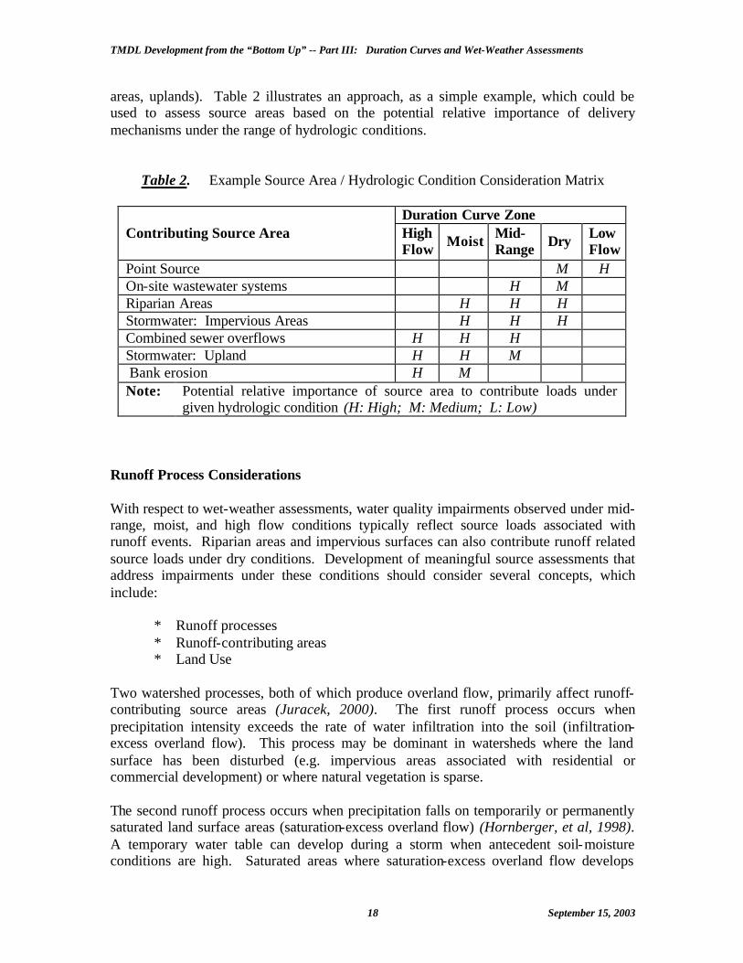
TMDL Development from the “Bottom Up” -- Part III: Duration Curves and Wet-Weather Assessments
18 September 15, 2003
areas, uplands). Table 2 illustrates an approach, as a simple example, which could be used to assess source areas based on the potential relative importance of delivery mechanisms under the range of hydrologic conditions.
Table 2. Example Source Area / Hydrologic Condition Consideration Matrix
Duration Curve Zone Contributing Source Area High
Flow Moist Mid-Range Dry Low
Flow Point Source M H On-site wastewater systems H M Riparian Areas H H H Stormwater: Impervious Areas H H H Combined sewer overflows H H H Stormwater: Upland H H M Bank erosion H M Note: Potential relative importance of source area to contribute loads under
given hydrologic condition (H: High; M: Medium; L: Low) Runoff Process Considerations With respect to wet-weather assessments, water quality impairments observed under mid-range, moist, and high flow conditions typically reflect source loads associated with runoff events. Riparian areas and impervious surfaces can also contribute runoff related source loads under dry conditions. Development of meaningful source assessments that address impairments under these conditions should consider several concepts, which include:
* Runoff processes * Runoff-contributing areas * Land Use
Two watershed processes, both of which produce overland flow, primarily affect runoff-contributing source areas (Juracek, 2000). The first runoff process occurs when precipitation intensity exceeds the rate of water infiltration into the soil (infiltration-excess overland flow). This process may be dominant in watersheds where the land surface has been disturbed (e.g. impervious areas associated with residential or commercial development) or where natural vegetation is sparse. The second runoff process occurs when precipitation falls on temporarily or permanently saturated land surface areas (saturation-excess overland flow) (Hornberger, et al, 1998). A temporary water table can develop during a storm when antecedent soil-moisture conditions are high. Saturated areas where saturation-excess overland flow develops

TMDL Development from the “Bottom Up” -- Part III: Duration Curves and Wet-Weather Assessments
19 September 15, 2003
expand during a storm and shrink during extended dry periods (Dunne, et al, 1975). Both runoff processes can be expected to affect water quality in streams, although possibly in different ways due to different flow paths. Table 3 illustrates an approach that could be used to connect watershed process considerations with identification of potential runoff-contributing source areas using a duration curve zone framework.
Table 3. Example Runoff Process Considerations
Duration Curve Zone Contributing Source Area
High Flows
Moist Conditions
Mid-Range Flows
Dry Conditions
Low Flows
Woodland S(H) S(M) Grassland S(H) S(M) Cropland S(H) I(H) I(M) Urban S(H) S(H) I(H) I(H) Riparian areas S(H) S(H) I(H) I(H) S(H): S(M): I(H): I(M):
Saturation-excess (High runoff potential) Saturation-excess (Medium runoff potential) Infiltration-excess (High runoff potential) Infiltration-excess (Medium runoff potential)
Use with Water Quality Models Duration curves provide a way to approach water quality assessments. Several examples have been used to illustrate how duration curves can be used to provide a context for analyzing ambient water quality data. The duration curve framework can also be used to examine information produced from a source loading analysis or from a water quality model, such as HSPF (Figure 12). Water quality values calculated with a dynamic model, for instance, can be associated with daily average flow rates. This information can be used to determine a corresponding flow duration interval, and then develop a load duration curve based on the model output. Load duration curves developed from model output provide an alternative method, which can be used for communicating information to watershed groups. A load duration curve derived from a water quality model can also be compared to a LDC based on ambient water quality data (Figure 13). This type of analysis can either confirm model assumptions or help prioritize source assessment needs. Looking at Figures 12 and 13, the model appears to overestimate loads under dry and low flow conditions, when compared to ambient water quality data. The model also appears to underestimate loads, when examining moist and mid-range flow conditions. Investigating this discrepancy should be a high source assessment priority, as it could affect management decisions regarding the most effective implementation strategies.

TMDL Development from the “Bottom Up” -- Part III: Duration Curves and Wet-Weather Assessments
20 September 15, 2003
Figure 12. Duration Curve Developed Using HSPF Output
Figure 13. LDC from Ambient Data for Comparison to Model Results

TMDL Development from the “Bottom Up” -- Part III: Duration Curves and Wet-Weather Assessments
21 September 15, 2003
Source Tracking Information The increased use of source tracking methods offers another opportunity to utilize a duration curve framework in prioritizing source assessment efforts. For example, bacteria source tracking (BST) data is being collected to determine the potential origin of pathogens observed in water quality samples. Duration curves provide another view of BST information, in a way that considers the hydrologic condition of the watershed and potential delivery mechanisms. Figure 14 depicts BST data using the Antibiotic Resistance Analysis (ARA) method. In this example, the sample point represents a unit area load (e.g. the estimated load divided by the drainage area) for purposes of comparing data from different sites in the watershed. Each point is also identified with source categories from ARA results (the letter on the left denotes the dominant source; the letters inside the parentheses denote other sources detected above a minimum threshold). The role of the duration curve framework for this application is to examine patterns. In Figure 14, BST patterns observed under mid-range and moist conditions can help prioritize follow-up wet-weather assessments. Conversely, BST patterns observed under dry and low flow conditions can help identify direct bacteria inputs to the stream.
Figure 14. BST Information Displayed Using Duration Curve Framework

TMDL Development from the “Bottom Up” -- Part III: Duration Curves and Wet-Weather Assessments
22 September 15, 2003
IDENTIFYING POTENTIAL SOLUTIONS A major advantage of the duration curve framework in TMDL development is the ability to meaningfully connect allocations to implementation efforts. Because the flow duration interval (FDI) provides a general indication of hydrologic condition (i.e. wet versus dry and to what degree), allocations and reduction targets can be linked to source areas, delivery mechanisms, and the appropriate set of management practices. The use of duration curve zones (e.g. high flow, moist, median flows, dry, and low flow) allows the development of allocation tables, which can be used to summarize potential implementation actions that most effectively address water quality concerns. Connections to Management Practices Development of wasteload allocations for continuous point source discharges is relatively straightforward using a duration curve framework, when compared to nonpoint sources. Consideration of pollution control measures is typically done in conjunction with NPDES permit development. Wasteload allocations (WLAs) can be expressed at one level across the entire duration curve, or WLAs may be tiered to specific flow levels and the corresponding flow duration interval. Nonpoint sources, on the other hand, present a much greater challenge because pollutants are transported to surface waters by a variety of mechanisms (e.g. runoff, snowmelt, groundwater infiltration). Nonpoint source management practices generally focus on source control and / or delivery reduction. Table 4 illustrates an approach, which could be used to assess management options in a way that considers the potential relative importance of hydrologic conditions using a duration curve framework. Application of the concept is illustrated in Figure 15.
Table 4. Example Management Practice / Hydrologic Condition Considerations
Duration Curve Zone Management Practice High
Flow Moist Mid-
Range Dry Low
Flow Point source controls M H H Septic system inspection M H H M CSO repair / abatement H H H SSO repair / abatement M H H Riparian buffers H H H Pasture management H H M Pet waste education & ordinances M H H Hobby farm livestock education H H M Note: Potential relative importance of practice effectiveness under given
hydrologic condition (H: High; M: Medium; L: Low)
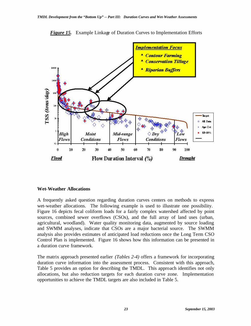
TMDL Development from the “Bottom Up” -- Part III: Duration Curves and Wet-Weather Assessments
23 September 15, 2003
Figure 15. Example Linkage of Duration Curves to Implementation Efforts
Wet-Weather Allocations A frequently asked question regarding duration curves centers on methods to express wet-weather allocations. The following example is used to illustrate one possibility. Figure 16 depicts fecal coliform loads for a fairly complex watershed affected by point sources, combined sewer overflows (CSOs), and the full array of land uses (urban, agricultural, woodland). Water quality monitoring data, augmented by source loading and SWMM analyses, indicate that CSOs are a major bacterial source. The SWMM analysis also provides estimates of anticipated load reductions once the Long Term CSO Control Plan is implemented. Figure 16 shows how this information can be presented in a duration curve framework. The matrix approach presented earlier (Tables 2-4) offers a framework for incorporating duration curve information into the assessment process. Consistent with this approach, Table 5 provides an option for describing the TMDL. This approach identifies not only allocations, but also reduction targets for each duration curve zone. Implementation opportunities to achieve the TMDL targets are also included in Table 5.

TMDL Development from the “Bottom Up” -- Part III: Duration Curves and Wet-Weather Assessments
24 September 15, 2003
Figure 16. Example CSO Allocation Using Duration Curve Framework
Table 5. Example TMDL Using Duration Curve Framework
High Moist Mid-Range Dry Low
Reduction 92% 90% 78% 40% 0%TMDL 1.39E+14 5.09E+13 2.37E+13 1.15E+13 5.09E+12
Load Allocations 9.32E+12 2.73E+12 2.26E+13 1.05E+13 4.22E+12Wasteload Allocations 4.68E+11 4.68E+11 4.68E+11 4.68E+11 4.68E+11
CSO 1.25E+14 4.58E+13 0.00E+00 0.00E+00 0.00E+00
Margin of Safety 4.11E+12 1.89E+12 6.20E+11 4.99E+11 4.06E+11
ImplementationOpportunities
Loads expressed as (cfu/day)
Long Term CSO Plan Municipal NPDESRiparian Protection
Pet Waste Ordinance
Stormwater Mgt.

TMDL Development from the “Bottom Up” -- Part III: Duration Curves and Wet-Weather Assessments
25 September 15, 2003
ADAPTIVE MANAGEMENT Duration curves provide a context for evaluating both monitoring data and modeling information. This offers another way to look at identifying data needs where adaptive management is being considered or utilized, particularly given the uncertainty associated with wet-weather situations. Specifically, adaptive management plays a key role in the implementation process for achieving load reductions. Using a value-added “bottom up” approach, TMDL development occurs using the best available data. Progress towards achieving load allocations are periodically assessed through phased implementation using measurable milestones. Adaptive management must be built into the process from the beginning. If a TMDL process or design does not have a component that can incorporate mid-course corrections, uncertainty and the differing views people have on it will hamper success (Poole, 2001). Developing a policy that incorporates adaptive management can help resolve the problem. Under adaptive management, a watershed plan should not be held up due to a lack of data and information for the “perfect solution”. The process should use an iterative approach that continues while better data are collected, results analyzed, and the watershed plan enhanced, as appropriate. Thus, implementation can focus on a cumulative reduction in loadings under a plan that is flexible enough to allow for refinement, which better reflects the current state of knowledge about the system and is able to incorporate new, innovative techniques. SUMMARY A “bottom up” approach is one way to establish a meaningful, value-added framework linking water quality concerns to proposed solutions. TMDL development using a “bottom up” approach considers the interaction between watershed processes, disturbance activities, and available methods to reduce pollutant loadings, specifically BMPs. A “bottom up” approach also capitalizes on the networks of programs and authorities across jur isdictional lines. Information on management measures related to both source control and delivery reduction methods can be incorporated into the allocation part of TMDL development. An advantage of the duration curve framework is its ability, as a simple communication tool, to link potential implementation efforts to the hydrologic condition of the watershed and to improve targeting of watershed restoration activities. The approach can examine relationships between source area / delivery mechanisms (e.g. point source discharges, storm-event runoff) and the corresponding watershed response, in a way that accounts for the range of different hydrologic conditions. A duration curve framework can support TMDL development intended to address wet-weather problems by characterizing water quality concerns, linking concerns to key watershed processes, prioritizing source assessment efforts, and identifying potential solutions.

TMDL Development from the “Bottom Up” -- Part III: Duration Curves and Wet-Weather Assessments
26 September 15, 2003
Flow duration intervals can be used as a general indicator of hydrologic condition (i.e. wet versus dry and to what degree). Flow duration curve intervals can be grouped into several broader categories or zones, in order to provide insight about conditions and patterns associated with the impairment. Flow duration zones can also be used to develop a matrix approach for developing water quality assessments. Duration curve zones can help point problem solution discussions towards relevant watershed processes, important contributing areas, and key delivery mechanisms. These are all important considerations when identifying those controls that might be most appropriate and under what conditions. Because of the potential utility as a diagnostic indicator and as a communication tool for targeting in the TMDL process, duration curves also provide a context for evaluating both monitoring data and modeling information. Water quality monitoring data used in a duration curve framework can support watershed planning by providing a better description of water quality concerns, improving the basic understanding of key watershed processes, and focusing solution development. This offers another way to look at identifying data needs where adaptive management is being considered or utilized. REFERENCES Bonta, J.V. March 2002. Framework for Estimating TMDLs with Minimal Data. ASAE
Proceedings of the Watershed Management to Meet Emerging TMDL Regulations Conference. Fort Worth, TX. pp. 6-12.
Cleland, B.R. November 2002. TMDL Development From the “Bottom Up” – Part II:
Using Duration Curves to Connect the Pieces. National TMDL Science and Policy 2002 -- WEF Specialty Conference. Phoenix, AZ.
Cleland, B.R. March 2001. Forestry and Agricultural BMP Implementation: TMDL
Development from the “Bottom Up”. ASIWPCA / ACWF / WEF TMDL Science Issues Conference: On-site Program. St. Louis, MO. pp 91-92.
Dunne, T., T.R. Moore, and C.H. Taylor. 1975. Recognition and Prediction of Runoff-
producing Zones in Humid Regions. Hydrological Sciences Bulletin. V.20, p 305-327.
Hornberger, G.M., J.P. Raffensperger, P.L. Wiberg, and K.N. Eshleman. 1998. Elements
of Physical Hydrology. Johns Hopkins University Press. Baltimore, MD. 302 p. Juracek, K.E. 2000. Estimation and Comparison of Potential Runoff-Contributing Areas
in Kansas Using Topographic, Soil, and Land-Use Information. U.S. Geological Survey Water Resources Investigations Report 00-4177. Lawrence, KS. 55 p.
Leopold, L.B. 1994. A View of the River. Harvard University Press. Cambridge, MA.

TMDL Development from the “Bottom Up” -- Part III: Duration Curves and Wet-Weather Assessments
27 September 15, 2003
Mehan, G.T. November 2001. Testimony on TMDL Program before Subcommittee on Water Resources and Environment – U.S. House of Representatives. Washington, DC.
Poole, W.C. June 2001. Uncertainty and Adaptive Management . ASIWPCA
STATEments. Washington, D.C. pp 5-6. Sheely, L.H. July 2002. Load Duration Curves: Development and Application to Data
Analysis for Streams in the Yazoo River Basin, MS. Special Project – Summer 2002. Jackson Engineering Graduate Program.
Sloto, R.A. and M.Y. Crouse 1996. HYSEP: A Computer Program for Streamflow
Hydrograph Separation and Analysis. U.S. Geological Survey Water Resources Investigations Report 96-4040. Lemoyne, PA. 46 p.
Stiles, T.C. November 2002. Incorporating Hydrology in Determining TMDL Endpoints
and Allocations. National TMDL Science and Policy 2002 -- WEF Specialty Conference. Phoenix, AZ.
Stiles, T.C. March 2001. A Simple Method to Define Bacteria TMDLs in Kansas.
ASIWPCA / ACWF / WEF TMDL Science Issues Conference: On-site Program. St. Louis, MO. pp 375-378.
Sullivan, J.A. March 2002. Use of Load Duration Curves for the Development of
Nonpoint Source Bacteria TMDLs in Texas. ASAE Proceedings of the Watershed Management to Meet Emerging TMDL Regulations Conference. Fort Worth, TX. pp. 355-360.
U.S. Environmental Protection Agency. October 1999. Protocols for Developing
Sediment TMDLs – First Edition. EPA 841-B-99-004. Washington, DC.

This page intentionally left blank

Appendix C
TMDL Implementation Plan for Vermilion River Watershed


C-i
Table of Contents Implementation Actions for Fecal Coliform in the Vermilion River (DS-06) ............................... 1
Point Sources .............................................................................................................................. 1 NPDES Permitted Facilities .................................................................................................... 1 Fecal Coliform Chlorination Exemptions ............................................................................... 3
Vermilion River Watershed Exemptions ............................................................................ 4 Combined Sewer Overflows (CSOs) ...................................................................................... 5
Fairbury’s Long Term Control Plan Information ............................................................... 7 Individual Homeowner Failing Septic Systems ...................................................................... 8 Livestock in Streams ............................................................................................................... 9
Nonpoint Sources ...................................................................................................................... 10 Septic System Failures .......................................................................................................... 10 Land Application of Manure ................................................................................................. 11
Pathogen Reduction- Manure Collection and Storage ...................................................... 11 Manure Management Plans............................................................................................... 16
Implementation Actions for Nitrate in the Vermilion River (DS-06, DS-10 and DS-14) ............ 17 Point Sources ............................................................................................................................ 17 Application Timing/Inhibitors .................................................................................................. 17 Wetlands ................................................................................................................................... 17 Nutrient Management Plans ...................................................................................................... 20
Nutrient Management Plans in TMDL Watersheds- ........................................................ 23 Tile Drainage Water Management ............................................................................................ 24 Tile Drain Biofiltration (Subsurface Bio-reactors) ................................................................... 25
References ..................................................................................................................................... 27
Figures Figure 1. Point Sources with Fecal Limits ..................................................................................... 2 Figure 2. Point Sources with Chlorination Exemption .................................................................. 4 Figure 3. CSOs in the Watershed ................................................................................................... 6 Figure 4. Hydric Soils in the Vermilion Watershed .................................................................... 18
Tables Table 1. NPDES Facilities with Sanitary Waste Discharge and Fecal Coliform Data .................. 1 Table 2. Facilities and Exemption Status ....................................................................................... 4 Table 3. Chlorination Exemption Information............................................................................... 5 Table 4. CSO Permit Information ................................................................................................... 5 Table 5. Treated CSO Discharge ................................................................................................... 6 Table 6. CSO DMR Data from January 2002 through December 2007 ........................................ 6 Table 7. Untreated CSO Discharges .............................................................................................. 7 Table 8. Estimate Septic Tank Pumping Frequencies in Years ................................................... 10

C-ii
This page left blank for double-sided printing

C-1
Implementation Actions for Fecal Coliform in the Vermilion River (DS-06) Both point and nonpoint sources of fecal coliform need to be reduced in the watershed. All the flow regimes need reductions especially at high flows which require a 91 percent reduction (Table 23 in the Stage 3 of this TMDL Report). Point sources that need to be considered for this TMDL are NPDES permitted facilities that are not in compliance of their permit limits, NPDES facilities that are exempt from disinfections and monitoring of fecal coliform, combined sewer overflows (CSOs), rural sewage directly discharging to streams and livestock waste runoff discharging into streams. Nonpoint sources of fecal coliform are runoff that includes sources from livestock waste, pets, wildlife, septic failures, and biosolids applications. Point Sources NPDES Permitted Facilities There are fifteen facilities in the watershed that discharge fecal coliform in their effluent and four of those facilities have permit limits- Oglesby, Streator, Pontiac and Stelle Community Association. Only Pontiac and Stelle Community Association discharge to segment DS-06 or upstream of this segment. Pontiac STP has a seasonal fecal coliform exemption and therefore is required to disinfect and monitor during the swimming months of May through October. Stelle Community Association STP (subdivision) has no exemption in the watershed and is required to monitor for fecal coliform all year to demonstrate compliance. They are required to submit monthly discharge monitoring report (DMR) data to Illinois EPA. There are four year-round exempted facilities in the watershed that do not have to chlorinate or monitor at any time during the year (more exemption information is in the next section). Table 1 contains facilities that could contribute fecal coliform to segment DS-06. The table includes permit ID, permit expiration date, the designed average flow (DAF), the geometric mean of seasonal fecal coliform data and the maximum concentration that resulted in an exceedence of the standard. Table 1. NPDES Facilities with Sanitary Waste Discharge and Fecal Coliform Data
NPDES Facility Permit ID Expiration Date
DAF (MGD)
Effluent Data
Geo Mean (cfu/100 ml)
Violation Maximum (cfu/100ml)
Pontiac STP IL0030457 9/30/09 3.50 67 185 Stelle Community Assn STP IL0026697 1/31/11 0.04 3573 60,000
Pontiac STP Pontiac is in compliance with the fecal coliform permit limit. Pontiac STP discharges into segment DS-06, but is downstream of the monitoring site and therefore would not affect data for this segment.

C-2
Figure 1. Point Sources with Fecal Limits
Stelle Community Association STP Stelle Community Association Sewage Treatment Plant is not in compliance of the fecal coliform limits. The table below has monthly monitoring data. The facility should be discharging under 400 cfu/100ml.
Date Fecal coliform (cfu/100ml)
8/31/2007 400 9/30/2007 1011
10/31/2007 400 11/30/2007 60000 12/31/2007 60000 1/31/2008 60000 2/28/2008 400 3/31/2008 400 4/28/2008 400 5/31/2008 60000

C-3
Subdivisions- Homeowner Maintenance of Septic Systems Homeowners must maintain their own septic systems so that disinfection takes place. This usually involves adding chlorine tablets into their system to disinfect. Most systems require one tablet added to the system, checking the chlorinator once a month to determine how often to add tablets (depends on family size). Please see operating procedures for individual septic units or your county health department for maintenance instructions. Illinois EPA will work with Stelle Community Association for future compliance with the fecal coliform standard. Fecal Coliform Chlorination Exemptions Waters unsuited to support primary contact uses because of physical, hydrologic or geographic configuration and are located in areas unlikely to be frequented by the public on a routine basis as determined by the Agency at 35 Ill. Adm. Code 309.Subpart A, are exempt from the fecal coliform standard (35 Ill. Adm. Code 302.209 (b)). The facility must demonstrate it is an unprotected water of the State to obtain a year-round disinfection exemption under 35 Ill. Adm. Code 378.203. Unprotected waters are not required to comply with the fecal coliforms standards (35 Ill. Adm. Code 378.203). Characteristics of unprotected waters include but are not limited to the following, and waters must possess one or more of these characteristics to be classified as unprotected waters:
a) Waters with average depths of two feet or less and no pronounced deep pools during the summer season;
b) Waters containing physical obstacles sufficient to prevent access or primary contact activities; or
c) Waters with adjacent land uses sufficient to discourage primary contact activities. To demonstrate the unprotected status of the water, the permitee must assess the water (35 Ill. Adm. Code 378.204). The permittee shall conduct surveys necessary to determine whether affected waters currently support or have the potential to support primary contact activities. The permitee shall conduct surveys necessary to determine whether any affected waters which flow through or adjacent to parks or residential areas have the potential to attract the public and create a risk of incidental or accidental contact. Such waters are protected by the seasonal fecal coliform standard (limits for the recreational period of May through October) unless the permittee can demonstrate that access is limited by such impediments as fences or steep banks. The Agency must model the die-off of fecal coliform from its discharge to show that at the end of the unprotected water, the water is meeting the fecal coliform standard. The first order die-off equation and application of it may be found in 35 Ill. Adm. Code 378 Appendix A through E. The initial fecal coliform concentration used in the die-off equation is required to be used by the permittee. An average fecal coliform concentration of over at least 3 months is preferable, but a minimum of 4 samples in 30 days is acceptable.

C-4
Vermilion River Watershed Exemptions Illinois EPA is reexamining the disinfection exemption process in the state of Illinois. All dischargers within three miles of a fecal coliform impaired stream will have to reapply for disinfection exemption status. Within TMDL watersheds, facilities with exemptions will be evaluated and those with exemption reaches upstream of impaired streams may be asked to reapply for exemption status. Figure 2 shows the exempt facilities in the watershed. Only those facilities that discharge into the impaired segment or upstream may be contributing to impairment in segment DS-06. Table 2 lists the exempt facilities, the permit expiration date and the year the exemption was granted. Table 3 contains exemption information used in the die-off equations. All of these exemptions were granted in 1988 or 1989. Figure 2. Point Sources with Chlorination Exemption
Table 2. Facilities and Exemption Status NPID Facility Name Permit
Expiration Exemption Granted
ILG580091 Chatsworth STP 12/31/2007 1989 IL0021601 Fairbury STP 5/31/2009 1988 IL0028819 Forrest STP 8/31/2010 1988 IL0037001 Greenbriar Health Care 7/31/2011 1989

C-5
Table 3. Chlorination Exemption Information
NPID Facility Name DAF (MGD)
Average Discharge
Maximum Discharge
No. of Samples
Date Taken
ILG580091 Chatsworth STP 0.18 8,747 16,213 4 Jan/Feb-89 IL0021601 Fairbury STP 0.66 3,892 4,200 5 Sept- 88 IL0028819 Forrest STP 0.35 106 257 6 Aug-Oct- 87 IL0037001 Greenbriar Health Care 0.01 41,010 71,700 4 Jan-Feb- 89
Illinois EPA will reevaluate exemptions for this watershed during the permit renewal process. Recent monitoring data for die-off calculations and survey information may be required in the reevaluation process. Combined Sewer Overflows (CSOs) During wet weather events, the combined wastewater and stormwater runoff entering combined sewers systems (CSSs) may exceed the capacity and discharge directly to surface water during and after these events. There are CSOs that are treated and ones that are untreated. Untreated wastewater can contribute microbial pathogens and impact human health. Treated CSOs must sample during discharge and submit monthly DMR data. All combined sewer systems in the watershed are required to provide complete treatment for the first flush flows from a one-year one-hour storm event and to provide primary treatment and disinfection for at least ten times the average dry weather flow. Systems containing untreated CSOs that discharge four or more times a year are required to develop and submit a Long Term Control Plan (LTCP) that details how they will reduce the CSOs in the future. For more information on LTCPs and the technologies used to control CSOs, refer to Report to Congress: Impacts and Control of CSOs and SSOs (USEPA 2004). Fairbury, Forrest, and Pontiac discharge to the impaired stream segment or upstream. There are treated CSO discharges in Fairbury and Forrest. Treated CSOs are required to disinfect and monitor for fecal coliform when discharging (Table 5 and Table 6). There are untreated discharges in Fairbury and Pontiac (Table 7). Table 4. CSO Permit Information Facility Permit ID Permit Expires CSO Discharges LTCP Status Fairbury STP IL0021601 5/31/09 Untreated and Treated Received Dec 2006,
under revision. Forrest STP IL0028819 8/31/10 Treated N/A- no untreated
discharges Pontiac STP IL0030457 9/30/09 Untreated Received Jan 2009,
under revision.

C-6
Figure 3. CSOs in the Watershed
Table 5. Treated CSO Discharge STP Facility Outfall
Pipe Outfall Name Discharges
per Year Average Duration of Discharge
Average Volume (MG)
Receiving Stream
Fairbury STP 002 Excess Flow 5 1-20 days 1.056 Indian Creek Forrest STP A010 Excess Flow 2-5 N/A N/A S. Fk. Vermilion R. Table 6. CSO DMR Data from January 2002 through December 2007 STP Facility Outfall Months
w/ Data Months w/ Discharges
Months w/ Exceedences
Geo Mean cfu/100ml
Max cfu/ 100ml
Fairbury 002 72 30 0 195 394 Forrest A010 72 30 0 11 305 As for treated CSOs, neither Fairbury nor Forrest has exceeded the NPDES limit of 400 cfu/100 ml.

C-7
Table 7. Untreated CSO Discharges
NPDES Out-fall
Location Receiving Stream
NPDES Info Year
Discharg Per Year
Ave. Duration (Hours)
Ave. Discharg (MG)
Most Recent DMR Data
Discharg per Year
Ave. Duration (Hours)
Fairbury CSO
003 CSO-36" Plant Bypass
Indian Creek 2002 10 1.5 0.2 2006 3 0.93
004 So of Plant, Ash in fld Indian Creek 2002 25 1.25 0.3 2006 3 1.27 005 So of Plant, Mpl in fld Indian Creek 2002 16 2.5 0.01 2006 3 1.08 006 So of Plant, Lcst in fld Indian Creek 2002 23 2.5 0.03 2006 3 1.27 007 S. 7th St. A Indian Creek 008 S. 7th St B Indian Creek 2002 15 1 0.006 2006 3 0.97 009 S. 7th St. C Indian Creek 010 South Alley E. of 4th Indian Creek 011 S. 4th St Indian Creek 2002 24 1.5 0.01 2006 3 1.08 012 Removed
013 CSO-SOUTH FIRST STREET
Indian Creek 2002 18 1.5 0.008 2006 3 1.0
Pontiac CSO*
002 CSO located across river from STP
Vermilion R. 2003 7 1.41 2006 1 0.78
A02 CSO located across river from STP
Vermilion R. 2003 0 2006 1 0.9
004 North Street CSO N. Ditch to Verm
2003 10 0.84 2006 3 1.3
*Pontiac discharges downstream of monitoring station IEPA received Fairbury’s Long Term Control Plan by the due date of December 31, 2006. After the IEPA review, a revised plant of study was developed and approved. This will be used to develop a revised LTCP. Pontiac’s LTCP was due October 1, 2008. After an IEPA review a deficiency was found and Pontiac is currently revising the LTCP.
Fairbury’s Long Term Control Plan Information The following information was taken from the City of Fairbury’s Long Term Control Planning and Compliance with Water Quality Standards document.
Current Flow/Storage Capacity The current excess flow lagoon is sized for ten times the average dry weather flow and the mechanical plant is sized for 2.5 times the average dry weather flow. The existing treatment facility is able to contain and properly treat flows up to 12.5 average dry weather flows. The current staff of the treatment facility maximizes the storage within the excess flow lagoon by lowering the levels within it to provide maximum storage within it on a regular basis. The City is currently evaluating alternatives to monitor the ability of the collection system to transport flows to the treatment facility. New Construction Ordinances Current ordinances specify the use of storm water detention basins and separate storm sewers for any new construction, which reduce the amount of storm water that enters the system. Future Plans The City plans to design and construct underground storage structures for each of the CSOs on the south side of the City within six years after approval of the LTCP. They also plan to design and construct above-ground detention basins for the north CSOs within nine years of approval.

C-8
However, the City is also considering other treatment options, and what is actually built will depend on the cost and what improvements occur in the receiving waters.
Individual Homeowner Failing Septic Systems When a household is located beyond the city sewer system, all wastewater is typically treated and disposed of by an onsite septic system. The homeowner is responsible for providing care and maintenance. There are approximately 139,500 surface discharging systems in Illinois, with the potential of discharging 70 million gallons of sewage a day. Current test results suggest that between 20 and 60 percent of these systems are failing or have failed (IEPA 2004). Half of systems are over 30 years old and are more likely to malfunction (USDoC 1997). There are two primary treatment systems used- subsurface and surface systems. A surface discharging system discharges waste water directly to the ground’s surface, a natural drainage way, a collection tile, or a body of water. If it is not working properly, raw sewage can be discharged. Most surface discharging systems are aerobic systems. Wastewater from the home goes into a tank that has a compressor to push air through the waters so that aerobic bacteria decompose the organic material. Solids settle to the bottom and wastewater flows through a chlorine dispenser to inactivate any remaining bacteria before it is discharged. These systems are more complicated than subsurface systems and require more maintenance. County health departments manage all homeowner septic systems. They inspect any new system installed and respond to complaints of failing septic systems. The county health department can also be contacted on maintenance procedures for homeowners. Some county and local governments within Illinois have seen the negative effects that failing systems are having on their communities and have taken steps to voluntarily regulate these systems. Some address the installation of new private sewage systems for proposed subdivisions through established zoning or planning entities. Others have developed operation, maintenance and/or testing regulations for all surface discharging systems within their jurisdictions. For all septic issues, please contact your county health department or go to their website for more information.
County Health Department
Phone Number Web Address
Ford-Iroquois (815) 432-2483 http://www.fiphd.org/programs/environmental-health LaSalle 1-800-247-5243 http://www.lasallecounty.org/hd/index.htm Livingston (815) 844-7174 http://www.lchd.us/sewage%20&%20water.htm Marshall (309) 679-6000 McLean (309) 888-5450 http://www.mcleancountyil.gov/health/Environmental_Health.htm Woodford (309) 467-3064 http://www.woodfordhealth.org/wellSeptic.php
Illinois EPA attempted to issue a general NPDES permit for surface-discharge septic systems in June of 2007. The permit was sent for USEPA federal approval, but was objected because USEPA wants a prohibition of discharging septic tank systems in certain soil types. Since Illinois EPA does not approve septic tank systems for primate home, but rather this is a function that the General Assembly has given to the Illinois Department of Public Health (IDPH) through the Private Sewage Disposal Act, Illinois EPA has no way of enforcing this provision. The general permit was sent back to USEPA with a request that

C-9
they work with the IDPH to address this issue. Currently, USEPA and IDPH are working to revise regulations to address the remaining issue regarding soil types. Livestock in Streams To eliminate the direct discharge of livestock to a stream, restricting livestock using fencing, combined with alternative watering systems, may be used in the watershed. Possible funding for these projects may be available from the Environmental Quality Incentives Program (EQIP). Environmental Quality Incentives Program EQIP provides a voluntary conservation program for farmers and ranchers that promotes agricultural production and environmental quality as compatible national goals. EQIP offers financial and technical help to assist eligible participants install or implement structural and management practices on eligible agricultural land. EQIP offers contracts with a minimum term that ends one year after the implementation of the last scheduled practices and a maximum term of ten years. These contracts provide incentive payments and cost-shares to implement conservation practices. Persons who are engaged in livestock or agricultural production on eligible land may participate in the EQIP program. EQIP activities are carried out according to an environmental quality incentives program plan of operations developed in conjunction with the producer that identifies the appropriate conservation practice or practices to address the resource concerns. The practices are subject to NRCS technical standards adapted for local conditions. The local conservation district approves the plan. EQIP may cost-share up to 75 percent of the costs of certain conservation practices. Incentive payments may be provided for up to three years to encourage producers to carry out management practices they may not otherwise use without the incentive. However, limited resource producers and beginning farmers and ranchers may be eligible for cost-shares up to 90 percent. Farmers and ranchers may elect to use a certified third-party provider for technical assistance. An individual or entity may not receive, directly or indirectly, cost-share or incentive payments that, in the aggregate, exceed $450,000 for all EQIP contracts entered during the term of the Farm Bill. EQIP sign-up information is available online- http://www.nrcs.usda.gov/programs/eqip/ . Click on the State where your farm or ranching interest is located. This will take you to the application information for that State, the official ranking criteria used to evaluate your application, and a link to the form CCC-1200, Application for Participation and/or Contract.

C-10
Nonpoint Sources Nonpoint sources in the watersheds include failing septic systems, land application of biosolids, wildlife and livestock. Septic System Failures As mentioned previously, there are septic systems that discharge directly to the stream and there are also systems that discharge to the surface and subsurface. When failures take place, these can discharge untreated sewage on the surface, which can be transported to a stream by precipitation. A subsurface discharging system discharges waste underground. The system consists of two main parts- a septic tank and a soil absorption system (drainfield). Wastewater flows from the home into the tank where it stays long enough for the solids and liquids to separate. Solids lighter than water, such as grease, float to the top forming a layer of scum and heavier solids settle to the bottom as sludge. The middle layer flows from the tank to the drainfield where bacteria consume the pollutants contained in the sewage before it reaches groundwater. The scum and sludge in the septic tank need to be pumped out periodically to prevent back-ups. Pump the tank based on the size of the tank and the number of people using it. Table 8 is a guide for routine septic tank pumping. Pumping a 500 gallon tank usually costs between $150-200. If the tank does not get pumped, solids can pass through and clog the drainfield. Table 8. Estimate Septic Tank Pumping Frequencies in Years Tank Size (gal) Household Size (Number of People)
1 2 3 4 5 6 7 8 9 10
500 5.8 2.6 1.5 1 0.7 0.4 0.3 0.2 0.1 —
750 9.1 4.2 2.6 1.8 1.3 1 0.7 0.6 0.4 0.3
1000 12.4 5.9 3.7 2.6 2 1.5 1.2 1 0.8 0.7
1250 15.6 7.5 4.8 3.4 2.6 2 1.7 1.4 1.2 1
1500 18.9 9.1 5.9 4.2 3.3 2.6 2.1 1.8 1.5 1.3
1750 22.1 10.7 6.9 5 3.9 3.1 2.6 2.2 1.9 1.6
2000 25.4 12.4 8 5.9 4.5 3.7 3.1 2.6 2.2 2
2250 28.6 14 9.1 6.7 5.2 4.2 3.5 3 2.6 2.3
2500 31.9 15.6 10.2 7.5 5.9 4.8 4 4 3 2.6
Note: More frequent pumping needed if garbage disposal is used.
http://ohioline.osu.edu/aex-fact/0740.html When a system fails, homeowners may notice their plumbing draining slow and drain problems that continue after clog removal. Sewage can sometimes back up into the drains. Failure may also result in an overflow of sewage about the drainfield during large-volume discharges. Here are a few issues when dealing with subsurface septic systems:
• Flushing any foreign object into the septic tank (e.g., sanitary napkins, diapers) can cause problems to occur in the seepage field.
• When the tank is pumped out, the septic contractor should clean out the effluent filter. This filter stops the larger solids from getting out to the drainfield.

C-11
• Washing machines can be the cause of failure because of the lint generated. This gets flushed out to the drainfield where it plugs up the pores of the soil bed. To make matter worse, more clothing is made up of synthetic materials such as polyester and nylon which will not break down in a septic system. Lint can be prevented from entering the septic system by using a reusable, inline filter which attaches to your washing machine discharge hose.
• Excessive water use can flood your septic system and stir up and flush solids into the drainfield. Space out water use throughout the day and week. Try not to do all the laundry in one day. Water softeners can damage your system by putting too much water through the system. Newer efficient models use less water and regenerates on demand or a mini septic system can be installed for your softener. Water conserving fixtures like low flow showerheads and low flow toilets can also conserve water.
• Good surface drainage is important in the area of the seepage field. Do not drive over the field or this can cause compaction which will prevent natural evaporation of the effluent in the soil. Do not plant trees or shrubs near the seepage field. Do not put pavement or concrete on seepage fields. Divert any surface discharge (e.g.,gutter drainage) away from field.
Land Application of Manure Intensive animal confinement facilities have greater output or manure per facility than open grazing farms. The production facility may have little access to owned or rented land for feed production or waste disposal. Transportation of manure is costly, so the amounts disposed on nearby acreage may exceed crop requirements. The quantity of microorganisms in the application depends on precipitation, soil, vegetation, slope, application method, temperatures, and other factors. Manure storage is an important factor in reducing the bacteria content of manure to be applied to agricultural land and results in reduced levels in bacteria in runoff from the land where it is applied (Meals & Braun 2005). Manure application several days in advance of rain events can significantly reduce bacteria in runoff also. Although it is not possible to predict all weather events, it is possible to avoid application in advance of major storm events. Manure Management Plans have calculation and mapping tools, online confidential records and automatic reminders to make management easier for producers. Below is information on Best Management Practices from the University of Minnesota Extension at http://www.extension.umn.edu/distribution/livestocksystems/DI8544.html -
Pathogen Reduction- Manure Collection and Storage
Production Management
Use of vegetative filter strips. Runoff and erosion from open feedlots and manured fields can be routed through grass filter strips to remove sediment, nutrients, and bacteria. The effectiveness of vegetative filters at removing pollutants and microorganisms depends upon site characteristics such as slope, amount of runoff, type of wastes, and presence or absence of concentrated flows. Time of year is also important. The vegetative filter strips will be less effective during springtime snowmelt when the filter strips may still be frozen or not actively growing. One study has shown that grass filter strips (15 to 30 feet in length) remove 75 to 91% of fecal coliforms and 68 to 74% of fecal streptococci from runoff obtained from manured plots.[27] Animal confinement areas should have a 66 to 99 foot vegetative filter strip between animals and surface water in order to minimize contamination.[28]

C-12
Control runoff and leaching from stockpiled manure. Some livestock operations need to stockpile manure before land application. If manure must be stockpiled, producers should follow all regulations set by the state regulatory authority. Some states require that stockpiles be located, constructed, and operated so that manure-contaminated runoff from the site does not discharge into waters of the state. Permanent stockpiles must be placed on a concrete pad or clay base and have at least two feet of separation distance between the base of the stockpile and the seasonal high-water table. Catch basins can be used to prevent runoff from permanently stockpiled manure from reaching surface water.
Control runoff and leaching from open lots. Catch basins can be used to contain manure-contaminated water from an open lot. The water collected in catch basins can be land-applied or further treated by running through vegetative filter strips.
Install clean-water diversion. Berms and ditches can be used to divert up-slope runoff and rain water from buildings away from open lots or other areas where manure may accumulate. Preventing this excess water from entering the lot or manure stockpile area will not only reduce pollution potential, but will also help keep these areas drier. Drier facilities can improve animal health, which in turn lowers pathogen levels in manure.
Eliminate or reduce livestock access to streams, rivers, lakes, or ponds. Fencing livestock away from open water is an effective method of improving water quality. Keeping animals away from open water will prevent urination and defecation in the stream which can lead to bacterial pollution. Animal health may also be improved through reduced exposure to water-transmitted diseases and foot rot. Alternative livestock water systems can replace direct, uncontrolled livestock access to streams, ponds, and lakes. These systems are described in the UM Extensionbulletin BU-07606, Grazing Systems Planning Guide, available in paper or in electronic form at www.extension.umn.edu.
Best management practices to control runoff from livestock operations will not eliminate or reduce pathogens on a livestock operation. However, implementation of these BMPs will prevent pathogens from leaving the livestock operation and potentially contaminating food or water supplies. Most are relatively easy to install and partial funding for construction of systems to control or treat runoff may be available through the Natural Resource Conservation Service Environmental Quality Incentives Program (NRCS – EQIP) or state cost-share programs. Contact your local NRCS office or Soil and Water Conservation District to determine if your project qualifies for EQIP or other cost-share programs.
Biological Treatment of Manure Anaerobic storage. Anaerobic lagoons are widely used in southern climates for the treatment and temporary storage of swine manure. Deep pits, also an anaerobic storage system, located beneath animal housing facilities, are commonly used. In an anaerobic system, bacteria are not exposed to oxygen. Although bacteria can survive anaerobic conditions for long periods of time, most pathogens are reduced within 30 days.[29] Bacteria that do survive may be destroyed during the land application process due to exposure to UV light and the natural drying out of the bacteria if the manure is surface applied. However, it is recommended that liquid manure from these systems be injected or immediately incorporated to conserve nitrogen and avoid risk of phosphorus runoff.
Composting.Compost is an organically rich soil amendment produced by the decomposition of organic materials. During the composting process, organic materials such as animal manure and livestock carcasses are broken down by microorganisms. Active composting generates heat, carbon dioxide (CO2) and water vapor. The end product of composting is a dark, earthy-smelling
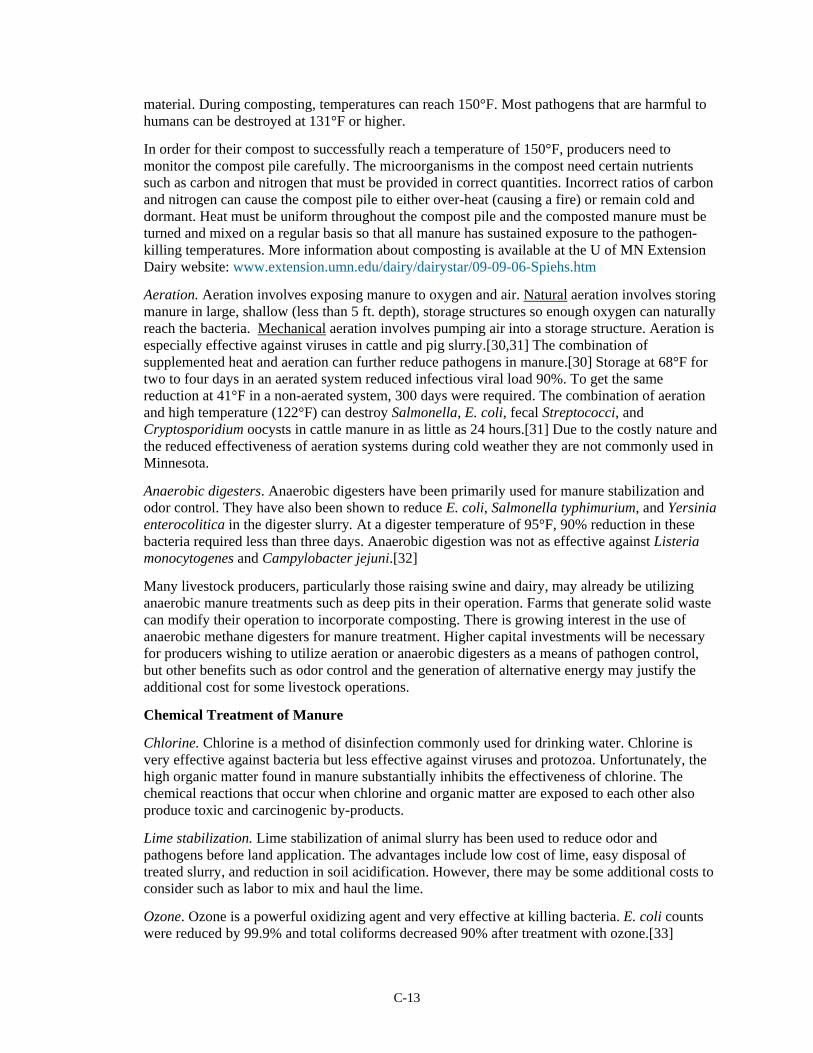
C-13
material. During composting, temperatures can reach 150°F. Most pathogens that are harmful to humans can be destroyed at 131°F or higher.
In order for their compost to successfully reach a temperature of 150°F, producers need to monitor the compost pile carefully. The microorganisms in the compost need certain nutrients such as carbon and nitrogen that must be provided in correct quantities. Incorrect ratios of carbon and nitrogen can cause the compost pile to either over-heat (causing a fire) or remain cold and dormant. Heat must be uniform throughout the compost pile and the composted manure must be turned and mixed on a regular basis so that all manure has sustained exposure to the pathogen-killing temperatures. More information about composting is available at the U of MN Extension Dairy website: www.extension.umn.edu/dairy/dairystar/09-09-06-Spiehs.htm
Aeration. Aeration involves exposing manure to oxygen and air. Natural aeration involves storing manure in large, shallow (less than 5 ft. depth), storage structures so enough oxygen can naturally reach the bacteria. Mechanical aeration involves pumping air into a storage structure. Aeration is especially effective against viruses in cattle and pig slurry.[30,31] The combination of supplemented heat and aeration can further reduce pathogens in manure.[30] Storage at 68°F for two to four days in an aerated system reduced infectious viral load 90%. To get the same reduction at 41°F in a non-aerated system, 300 days were required. The combination of aeration and high temperature (122°F) can destroy Salmonella, E. coli, fecal Streptococci, and Cryptosporidium oocysts in cattle manure in as little as 24 hours.[31] Due to the costly nature and the reduced effectiveness of aeration systems during cold weather they are not commonly used in Minnesota.
Anaerobic digesters. Anaerobic digesters have been primarily used for manure stabilization and odor control. They have also been shown to reduce E. coli, Salmonella typhimurium, and Yersinia enterocolitica in the digester slurry. At a digester temperature of 95°F, 90% reduction in these bacteria required less than three days. Anaerobic digestion was not as effective against Listeria monocytogenes and Campylobacter jejuni.[32]
Many livestock producers, particularly those raising swine and dairy, may already be utilizing anaerobic manure treatments such as deep pits in their operation. Farms that generate solid waste can modify their operation to incorporate composting. There is growing interest in the use of anaerobic methane digesters for manure treatment. Higher capital investments will be necessary for producers wishing to utilize aeration or anaerobic digesters as a means of pathogen control, but other benefits such as odor control and the generation of alternative energy may justify the additional cost for some livestock operations.
Chemical Treatment of Manure
Chlorine. Chlorine is a method of disinfection commonly used for drinking water. Chlorine is very effective against bacteria but less effective against viruses and protozoa. Unfortunately, the high organic matter found in manure substantially inhibits the effectiveness of chlorine. The chemical reactions that occur when chlorine and organic matter are exposed to each other also produce toxic and carcinogenic by-products.
Lime stabilization. Lime stabilization of animal slurry has been used to reduce odor and pathogens before land application. The advantages include low cost of lime, easy disposal of treated slurry, and reduction in soil acidification. However, there may be some additional costs to consider such as labor to mix and haul the lime.
Ozone. Ozone is a powerful oxidizing agent and very effective at killing bacteria. E. coli counts were reduced by 99.9% and total coliforms decreased 90% after treatment with ozone.[33]

C-14
However, organic materials found in animal waste interfere with ozonation and therefore a pretreatment such as solids separation would be needed for an effective ozonation process.
Ultraviolet light (UV) irradiation. Ultraviolet light irradiation destroys the DNA and RNA of pathogens. There are no residual compounds present after UV disinfection and the nutrient content of manure is not affected by UV exposure. Viruses are more resistant to UV treatment than bacteria and protozoa.
Pasteurization. Pasteurization of manure requires that a temperature of 158°F be maintained for 30 minutes. It is effective at reducing all pathogens but would be cost-prohibitive on most livestock operations unless it occurs as part of a composting or digesting system.
While effective in reducing pathogen levels in stored manure, most chemical treatments are not economically feasible for small to mid-sized livestock producers. Lime stabilization may be the only chemical treatment that could be implemented economically on small or mid-sized farms. However, larger producers may find chemical treatments such as ozone an attractive alternative to current manure management practices.
Pathogen Runoff- Land Application
Land application is a critical period in manure management. Pathogens from animal waste can threaten humans who are exposed to runoff, have direct contact with manure, or consume food or water contaminated with infectious manure. Application rate and seasonal conditions are important factors contributing to the transfer of pathogens from lands where manure has recently been applied to nearby surface water.
There is a higher risk of pathogen transfer to the food chain when fresh manure is land-applied than when stored manure is land-applied because there is no storage or treatment period to decrease pathogen numbers.[34] Typically, bacteria are highly susceptible to UV light and drying that naturally occur following surface application of manure to cropland. Cattle grazed on pasture two to three weeks after human sludge was applied to a field did not get sick but 1/3 of cattle that grazed a field immediately after sludge application became ill with Salmonella.[35] This indicates that pathogen numbers were decreased by UV exposure and natural drying of manure on the soil surface. Delaying incorporation for even one week significantly reduced pathogen survival following manure application due to exposure to UV radiation and the drying effect of the atmosphere.[36] Incorporating manure will increase the total time that manure-borne pathogens remain viable in the soil after land application.[36] But leaving manure on the soil surface increases the likelihood that pathogens can spread through flies or vermin, increases the possibility that heavy rainfall will cause surface runoff and contaminate nearby water sources, and increases odor and gas emissions from the field.[36]
The greatest risk of pathogen transfer from manured land to surface waters is through runoff. Runoff into tile lines or surface fractures in Karst soils can contaminate ground water as well. Production practices that reduce or eliminate runoff of manure-contaminated water will ultimately reduce pathogen transfer. When it comes time to land-apply livestock manure, be sure to calibrate application equipment and apply at recommended rates based on crop nutrient needs. Manure application rate has been shown to correlate positively with indicator organisms for pathogenic viruses.[37] Higher levels of indicator organisms were found in soils where manure was applied at twice the recommended level compared to soils where manure was not applied.[36] These high levels persisted for 143 days after manure application.[37] Injection or incorporation of manure will also decrease runoff potential.[37,38] Avoid application during winter months when the ground is frozen because this increases the likelihood of manure runoff into nearby waters during spring snow melt. Pathogen survival in manure and soil is enhanced at

C-15
low temperatures[39], increasing the risk of transport of viable pathogens in surface runoff from winter-applied manure.
Resources for Additional Information
University of Minnesota Extension Manure Management and Air Quality www.manure.umn.edu Livestock and Poultry Environmental Stewardship www.lpes.org National Livestock and Poultry Environmental Learning Center www.lpe.unl.edu Minnesota Pollution Control Agency www.pca.state.mn.us Midwest Planning Service www.mwps.org
References from extension webpage 27. Coyne, M.S., R.A. Gilfillen, R.W. Rhodes, and R.L. Blevins. 1995. Soil and fecal coliform trappings by
grass filter strips during simulated rain. J. Soil Water Conserv. 50: 405-408. 28. Hubbard, R.K., J.A. Entry, and J.E. Thies. 1999. Movement of coliform bacteria through riparian buffer
systems receiving swine lagoon wastewater. 1999 ASAE Annual International Meeting, Paper No. 99-2100, ASAE. St. Joesph, MI.
29. Krieger, D.J., J.H. Bond, and C.L. Barth. 1975. Survial of Salmonella, total coliforms, and fecal coliforms in swine waste lagoon effluents. Page 11-14 in Proc. 3rd Int. Symp. Addressing Animal Production and Environmental Issues. Urbana-Champaign, IL.
30. Lund, E., and B. Nissen. 1983. The survival of enteroviruses in aerated and non-aerated cattle and pig slurry. Agric. Wastes. 7:221-233.
31. Oeschner, H., and L. Doll. 2000. Inactivation of pathogens by using the aerobic-thermophilic stabilization process. Pages 522 – 528 in Proc. 8th. Int. Symp. on Animal, Agricultural and Food Processing Wastes. Des Moines, IA.
32. Kearney, T.E., M.J. Larkin, and P.N. Levett. 1993. The effect of slurry storage and anaerobic digestion on survival of pathogenic bacteria. J. Appl. Bacteriol. 74: 86-93.
33. Watkins, B.D, S.M. Hengenuehle, H.L. Peterson, M.T. Yokoyama, and S.J. Masten. 1996. Ozonation of swine manure wastes to control odors and reduce concentrations of pathogens and toxic fermentation metabolites. Pages 379-386 in Proc. Int. Conf. on Air Pollution from Agricultural Operations. Kansas City, MO.
34. Nicholson, F.A., S.J. Groves, and B.J. Chambers. 2005. Pathogen survival during livestock manure storage and following land application. Bioresource Technol. 96:135-143.
35. Bicknell, S.R., 1972. Salmonella aberdeen infection in cattle associated with human sewage. J. Hyg. 70:121-126.
36. Hutchison, M.L, L.D. Walters, A. Moore, K.M. Crookes, and S.M. Avery. 2004. Effect of length of time before incorporation on survival of pathogenic bacteria present in livestock wastes applied to agricultural soil. Appl. Environ. Microbiol. 70:5111-5118.
37. Gessel, P.D., N.C. Hansen, S.M. Goyal, L.J. Johnston, and J. Webb. 2004. Persistence of zoonotic pathogens in surface soil treated with different rates of liquid pig manure. Appl. Soil. Ecol. 25:237-243.
38. Chalmers, R.M., H. Aird, and F.J. Bolton. 2000. Waterborne Escherichia coli O157:H7. J. Appl. Microbiol. 88:124S-132S.
39. Guan, T.Y. and Holley, R.A. 2003. Pathogen survival in swine manure environments and transmission of human enteric illness—a review. J. Environ. Qual. 32:383-392.

C-16
Manure Management Plans A manure management plan is a tool that producers can use to optimize crop production. It helps to identify the amount of manure produced, the nutrient concentration in the manure, the number of acres that is required for land application and the amount that will be applied to each available acre. In Illinois, there are three different manure management plans that a livestock facility might need to have. For example, larger feeding operation facilities and producers applying for EQIP funds require a plan. University of Illinois Extension has worked with Illinois Department of Agriculture, Illinois Natural Resources Conservation Service, and the Illinois Environmental Protection Agency to develop one website of step-by-step instructions that, if completed, will comply with the needs of all three agencies. The process is online at www.immp.uiuc.edu. Plans are password protected and can be accessed online. Some features of the online version include:
• Calculation tools to match manure application rates with crop needs and soil tests • Mapping tools to draw the farmstead with its features, including buildings and storages • Help with annual plan updates • Recordkeeping and report forms • A user-defined calendar that will send automatic email reminders for inspections and records • Individual plans are password-protected and reside on a U of I server for reliable storage and
instant retrieval on any computer with web access. (www.prairiefarmer.com)

C-17
Implementation Actions for Nitrate in the Vermilion River (DS-06, DS-10 and DS-14) There are point and nonpoint sources of nitrate, but in this watershed nonpoint sources are the main source of nitrates and will be the target of implementation. Segment DS-10 is the most downstream segment and requires a 31 percent reduction at high flows. The nonpoint nitrogen source of concern for this watershed is fertilizer applied to agricultural lands. There are steps that can be done to reduce fertilizer usage/runoff- spring application, increase wetlands, nutrient management and tile drainage management. Point Sources There are no monitoring limits for nitrate in the watershed. The allocations were based on facilities discharging 18 mg/L nitrate in their effluent based on book values of treatment plant effluent. Point sources are not considered a major issue in the watershed. Exceedences only occur during high to medium flow events in which point sources make up less than 1 percent of this flow. Application Timing/Inhibitors Changing the timing of fertilizer application from fall to spring can reduce nitrogen loss and increase efficiency. In a Minnesota study, spring application increased nitrogen efficiency by more than 20% and nitrate loss was reduced by 36% (Dinnes et al 2002). University of Illinois research has also shown that it can take 120 pounds of fall-applied nitrogen to produce the same yield increase as 100 pounds applied in the spring (Weinzierl et al 1996). For farmers who still apply in the fall, nitrification inhibitors, such as nitrapyrin, dicyandiamide and ammonium thiosulfate slow the conversion of ammonium to nitrate by affecting the soil bacteria. These can slow the conversion 2-6 weeks. Nitrification inhibitors can improve the effectiveness of fall-applied nitrogen, but spring applied is more effective than fall applied with an inhibitor when conditions favoring nitrogen loss from fall application develops (Bundy 1986). Wetlands Nitrogen fertilizer applied to cultivated crops is lost in agricultural drainage water primarily in the form of nitrate. Ammonia is applied to fields and converted into nitrate by nitrification. Nitrate is very soluble in water and easily transported in water. In much of the Corn Belt, the establishment of agricultural drainage networks (tiles) and the conversion of the natural landscape to annual cropping systems have resulted in increased flow rates and hydraulic loading to streams (Crumpton et al 2008). Most Illinois farmland has tile drains and buffer strips that reduce surface runoff/erosion, but do not have much of an effect on nitrate reduction. Wetlands can be used instead as a long term “sink” for nutrients where nitrate is denitrified. Using the Surgo Soil Information from the Department of Agriculture, hydric soils were mapped.

C-18
Figure 4. Hydric Soils in the Vermilion Watershed
Most of the soils in this watershed are hydric which is why tile drains are prevalent throughout this highly agricultural landscape. Biological activity in wetlands can be effective at removing nitrate by converting it. Under anaerobic conditions, nitrate is oxidized by denitrification, resulting in nitrogen gas loss or through dissimilatory reduction of nitrate to ammonium. When wetlands are subjected to significant external nitrate loading, relatively high rates of denitrification can be expected, and with rare exception, denitrification is cited as the primary reason wetlands serve as nitrogen sinks (Crumpton et al 2008). Wetlands intended to intercept diffuse agricultural nutrient loads are usually located in low-lying areas with hydric soils. For wetlands to be effective they must be positioned to intercept significant nutrient loads and be of sufficient size to allow adequate residence time to treat loads they receive (Crumpton et al 2008). Research conducted at the Iowa State University has demonstrated that wetlands have the potential to remove 40-90% of the nitrate in tile drainage from upper-lying croplands (http://www.fsa.usda.gov/FSA/newsReleases?mystate=ia&area=home&subject=copr&topic=crp-20&newstype=crpsuccessstories&type=detail&item=ss_ia_artid_618.html ).

C-19
More reference information on the Hydric Rating (NSSC 2008) This rating provides an indication of the proportion of the map unit that meets the criteria for hydric soils. Map units that are dominantly made up of hydric soils may have small areas, or inclusions, of nonhydric soils in the higher positions on the landform, and map units dominantly made up of nonhydric soils may have inclusions of hydric soils in the lower positions on the landform. Hydric soils are defined by the National Technical Committee for Hydric Soils (NTCHS) as soils that formed under conditions of saturation, flooding, or ponding long enough during the growing season to develop anaerobic conditions in the upper part (Federal Register, 1994). Under natural conditions, these soils are either saturated or inundated long enough during the growing season to support the growth and reproduction of hydrophytic vegetation. The NTCHS definition identifies general soil properties that are associated with wetness. In order to determine whether a specific soil is a hydric soil or nonhydric soil, however, more specific information, such as information about the depth and duration of the water table, is needed. Thus, criteria that identify those estimated soil properties unique to hydric soils have been established (Federal Register, 2002). These criteria are used to identify map unit components that normally are associated with wetlands. The criteria used are selected estimated soil properties that are described in "Soil Taxonomy" (Soil Survey Staff, 1999) and "Keys to Soil Taxonomy" (Soil Survey Staff, 2006) and in the "Soil Survey Manual" (Soil Survey Division Staff, 1993). If soils are wet enough for a long enough period of time to be considered hydric, they should exhibit certain properties that can be easily observed in the field. These visible properties are indicators of hydric soils. The indicators used to make onsite determinations of hydric soils are specified in "Field Indicators of Hydric Soils in the United States" (Hurt and Vasilas, 2006).
References: Federal Register. July 13, 1994. Changes in hydric soils of the United States. Federal Register. September 18, 2002. Hydric soils of the United States. Hurt, G.W., and L.M. Vasilas, editors. Version 6.0, 2006. Field indicators of hydric soils in the United States. Soil Survey Division Staff. 1993. Soil survey manual. Soil Conservation Service. U.S. Department of Agriculture Handbook 18. Soil Survey Staff. 1999. Soil taxonomy: A basic system of soil classification for making and interpreting soil surveys. 2nd edition. Natural Resources Conservation Service. U.S. Department of Agriculture Handbook 436. Soil Survey Staff. 2006. Keys to soil taxonomy. 10th edition. U.S. Department of Agriculture, Natural Resources Conservation Service.
The Conservation Reserve Program, Wetland Reserve Program and Wildlife Habitat Incentives Program can be used to put areas back into wetlands with cost and technical assistance.
Conservation Reserve Program http://www.nrcs.usda.gov/programs/crp/ Enrollment has been extended through September 30, 2012. The Farmable Wetland Program (FWP) was modified by expanding the land eligibility to include land on which a constructed wetland is to be developed to receive flow from an agricultural drainage system designed to provide nitrogen removal and other wetland function. Participants agree to restore hydrology of the wetland and establish vegetative cover. http://www.fsa.usda.gov/Internet/FSA_File/2008fbcrpsummary.pdf Wetlands Reserve Program http://www.nrcs.usda.gov/programs/wrp/states/il.html Since 1994, the Wetlands Reserve Program (WRP) has enrolled approximately 32,000 acres. Many landowners are interested in WRP because of the economical incentive to remove marginal fields from production to offset farm debt and re-invest the easement payment in more productive land and farm equipment. Although landowners' initial interest in WRP is primarily

C-20
economic, many have found a renewed interest in wildlife after the project is restored. For more information, please refer to the webpage above. Wildlife Habitat Incentives Program (WHIP) http://www.il.nrcs.usda.gov/programs/whip/index.html WHIP is a voluntary program for people who want to develop and improve habitat on private lands. It provides technical assistance and cost share payments. Participants agree to prepare and implementa a wildlife habitat development plan with help from the local conservation district. The agreement generally lasts from 5 to 10 years.
Nutrient Management Plans Midwestern fields frequently have a high degree of variability in soil nitate content from site to site within a singe field (Power et al 2000). So applying sufficient nitrogen fertilizers for high yields for productive areas can result in over fertilization of less productive areas. The following information is from Appendix A, Conservation Practices (CPP), Nutrient Management Plans- http://www.agr.state.il.us/Environment/LandWater/images/appendix-acpp.pdf
PURPOSE The purpose of the Nutrient Management Plan conservation practice, eligible under the CPP, is to assist agricultural landowners/operators in optimizing the application of nutrients for plant production, while minimizing offsite impacts to the environment and protecting water quality. PRACTICE STANDARD To be eligible for a CPP incentive payment, a Nutrient Management Plan must follow the USDA Natural Resources Conservation Service (NRCS) conservation practice standard for either Nutrient Management (Code 590) or Waste Utilization (Code 633). NRCS conservation practice standards for nutrient management plans include the University of Illinois, Illinois Agronomy Handbook recommendations for rate, timing and placement of nutrients and procedures for soil sampling and calculating yield potential. LAND ELIGIBILITY Eligibility is limited to agricultural land within a watershed approved by the Illinois Department of Agriculture. All cropland and pastureland that is actively used for producing an agricultural commodity or plant material is eligible for the Nutrient Management Plan conservation practice provided other eligibility and selection criteria are met. There is no limit on the number of acres that may be planned or receive an incentive payment. LANDOWNER/OPERATOR ELIGIBILITY Eligibility is limited to agricultural producers who own or operate agriculture land within high priority watersheds designated by the Illinois Department of Agriculture. Landowners/operators who meet program eligibility and selection criteria may receive a Nutrient Management Plan incentive payment one time only on the same farm, operating unit or acreage. INCENTIVE PAYMENTS An incentive payment of $5 per acre will be made by the SWCD to eligible and approved landowners/operators who develop and implement a Nutrient Management Plan. An additional $2 per acre will be paid by the SWCD to the approved plan preparer.

C-21
Landowners/operators with a reduced tillage system on cropland who are approved for development of a Nutrient Management Plan may receive a supplemental $2 per acre for performing a soil test for phosphorus in the upper 2 inches of the soil profile. All incentive payments will be made on a per acre basis. The number of acres that qualify for an incentive payment is based on the number of acres that directly benefit from the plan, and for which soil testing and other nutrient management information is prepared. APPLICATION Landowners/operators who are interested in the Nutrient Management Plan conservation practice may apply at the SWCD office in the county where the agricultural land is located. Form CPP-1 (Application/Contract/Payment Form), will be used to request the Nutrient Management Plan practice, along with other eligible conservation practices. If the conservation practice(s) is approved, Form CPP-1A (Agreement Terms and Conditions) will also be used. PRIORITIZATION Requests from landowners/operators for the Nutrient Management Plan conservation practice should be prioritized prior to selection and approval of financial incentives by the SWCD. Prioritization will ensure that the requests approved for funding will result in the most efficient use of state dollars for protecting water quality. The Phosphorus Assessment Procedure, found as an appendix in the NRCS Nutrient Management and Waste Utilization practice standards, should be used as a guideline in comparing the relative water quality benefits of requests for the Nutrient Management Plan conservation practice. Risk assessments that indicate a “high” or “medium” potential for the five site characteristic criteria, should have a higher potential for protecting water quality than one with a “low” assessment potential. Therefore, Nutrient Management Plan requests should be approved, first, for land that has a “high” risk potential. LANDOWNER RESPONSIBILITIES Upon approval and signing of CPP/NMP-1, CPP/NMP-2 and CPP-1A forms, the landowner/operator may proceed with making arrangements for preparation of a Nutrient Management Plan. The landowner/ operator is responsible for providing the necessary information for the plan regarding field and cropping history, previous fertility programs and crop yields. Following preparation of the Nutrient Management Plan, the landowners/operator is also responsible for fully implementing the plan. NUTRIENT MANAGEMENT PLAN PREPARER QUALIFICATIONS AND RESPONSIBILITIES Qualified Nutrient Management Plan preparers must be individuals who hold one or more of the following certifications:
• Certified Crop Advisor • Certified Crop Scientist • Certified Professional Crop Consultant • Certified Professional Agronomist • Certified Professional Soil Scientist
Qualified plan preparers must be certified by the USDA-NRCS as a “Third Party Vendor” for the development of nutrient management plans. Nutrient Management Plan preparers are responsible for preparing a plan that follows the NRCS conservation practice standards for Nutrient Management (Code 590) or Waste Utilization (Code 633), and contains all the information outlined in the “Plan Contents” section below. The 31 “Nutrient Management Plan” form (attached) must be fully completed and submitted to the SWCD for certification, before the landowner/operator may implement the plan. Following the implementation of the Nutrient

C-22
Management Plan by the landowner/operator, the plan preparer must certify that the plan was implemented, as planned, by completing the “Nutrient Management Plan Implementation Report” (attached). A copy of the Nutrient Management Plan Implementation Report must be submitted to the SWCD. NUTRIENT MANAGEMENT PLAN CONTENTS Nutrient management plans will include:
• Aerial site photographs or maps and a soils map. • Soil test results. Plans will be based on soil tests no older than 4 years. Soil samples will
be collected using the University of Illinois guidance and analyzed in an approved soil test laboratory. At a minimum, soil tests will include pH, phosphorus, and potassium.
• Current and/or planned crop rotation and appropriate legume credits for nitrogen. • Yield goals. Nutrient application rates will be based on amounts required for realistic
expected yields which will be calculated using the following method: 1. Use the actual yields for each field from the previous 5 years. 2. Discard any yields that differ more than 25% from the average yield. 3. Average the remaining yields and multiply by 1.05. 4. If yield records are not available for a field, select a realistic expected yield using the productivity index values given for the soil types in the field.
• Nutrient budgets for nitrogen, phosphorus, and potassium quantifying all nutrient sources (i.e., commercial fertilizer, manure, by-products, irrigation water, etc). The recommended rates will be based on the University of Illinois fertility recommendations outlined in the most recent edition of the Illinois Agronomy Handbook.
• Planned rates, methods, timing, and form of nutrient application. Indicate if P and/or K applications are for more than one crop year.
• Nutrient management plan needs to take into account elements of other plans; e.g., if the farmer is using no-till to meet conservation compliance requirements.
• Restrictions on nutrients being applied to frozen, snow covered, or saturated soil if the potential risk for runoff exists. Fall applications of nitrogen shall follow the guidelines in the most current version of the Illinois Agronomy Handbook.
• Location of sensitive areas (if present) and any nutrient management restrictions; e.g., around sink holes, wells, etc.
SWCD CERTIFICATION/PAYMENT Following the preparation of a Nutrient Management Plan by a qualified plan preparer, the plan must be certified as meeting the NRCS Nutrient Management Standard. The signature of a qualified NRCS or SWCD employee must be present on the plan, as well as the signatures of the landowner/operator and plan preparer. Upon receipt of the signed Nutrient Management Plan from the plan preparer, the SWCD may issue the $2 per acre payment to the plan preparer. Following implementation of the plan and upon receipt of the Nutrient Management Plan Implementation report, signed by an eligible plan preparer, the SWCD may issue the $5 per acre incentive payment (and $2 per acre supplemental payment, if approved), to the landowner/operator. REPORTING The Illinois Department of Agriculture may request periodic reports regarding the implementation of the Nutrient Management Plan practice.

C-23
Nutrient Management Plans in TMDL Watersheds- http://www.agr.state.il.us/Environment/LandWater/tmdl.html The Department of Agriculture shifted some resources to Soil and Water Conservation Districts (SWCDs) in TMDL watersheds to address agriculture impacts on water quality. These targeted funds are designated for incentive payments to landowners/ operators within that specific watershed to promote the use of management practices that reduce the movement of the specific pollutant causing the water quality impairment (see Illinois Department of Agriculture website above ). With nitrate as a cause, nutrient management plans will be eligible for incentive payment with these funds. This cost share is only available for land in TMDL watersheds. Eligible SWCDs are allocated funds based on their portion of the total number of cropland acres in the watershed.

C-24
Tile Drainage Water Management A control structure is placed at the outlet of a tile system to control the level of the water table in the soil. The goal is to provide enough drainage for good aeration and root development but to capture some of the water that would otherwise drain out under conventional systems (Frankenberger et al 2006). The water level can be raised after harvest to limit the water outflow thereby reducing nitrate delivery to drainage ditches and streams during the off-season (see insert on next page for average nitrate loads). Nitrates are kept in the fields and available to crops and over time, producers could potentially find the need for smaller quantities of applied fertilizers (Creamean 2003). It can also be raised after planting to create a potential to store water for the crop to use in midsummer, which has the potential to increase yields. Long term computer simulations indicate that the average annual yield increase is less than 5% but it could be substantial in some years (Cooke et al). This system does not imply less nitrogen needs to be applied to the field as the water along with nitrate leave by some other route. That flow path is longer and slower, giving more opportunity for denitrification or assimilation of the nitrate into organic nitrogen forms (Frankenberger et al 2006). The costs of the control structure vary. Existing drainage systems can be retrofitted for drainage water management by installing control structures at a cost of $50 to $100 per hectare (Cooke et al). For more information refer to- Purdue Extension Technical Bulletin 44: Drainage Watershed Management for the Midwest http://www.ces.purdue.edu/extmedia/WQ/WQ-44.pdf
(Frankenberger et al 2006)

C-25
Average Monthly Nitrate Load -Iroquois River-
Gauge Station near Chebanse, IL (1984-1998)
Source: STORET and USGS
The chart above shows the average monthly nitrate (NO3-N) load for the Iroquois River in eastern Illinois measured at Chebanse. This distribution is typical of central Illinois rivers and streams. The average annual N loss was measured to be about 19 lbs-N per acre. This is for all of land in the watershed (approximately 2,100 square miles). The cost of this nitrogen as fertilizer would be about $5,000,000 per year. About 50 percent of the nitrate load was delivered through the tile system to surface water during the fallow season (November 1 to April 1) when there is no production need for drainage to occur. Thus, total nitrate load could be appreciably reduced by fallow season tile flow management. Limiting the volume of water flowing through the tile drainage systems during times of the year when drainage is not needed can significantly reduce the amount of nitrogen lost from farmed fields. This information is from a NRCS Illinois Drainage Water Management Tour Brochure-http://www.spipipe.com/PDF/DWMTourBrochure.pdf (NRCS 2004).
Tile Drain Biofiltration (Subsurface Bio-reactors) In areas that are too flat to use wetlands for filtration, biofiltration can be used. Wood chip biofilters, or bio-reactors remove nitrates from tile drainage water without removing cropland from production. Bioreactors consist of wood chips and gravel media, placed underground, through which tile water is allowed to flow. These systems provide an alternative pathway and are designed so that there is no decrease in drainage effectiveness. The outlet of the bio-reactor is placed lower than the level of the existing tile, so water will more likely follow this pathway. However, should the flow capacity of the bio-reactor be exceeded, the water will pass through the existing tile outlet. Information about bio-reactors-
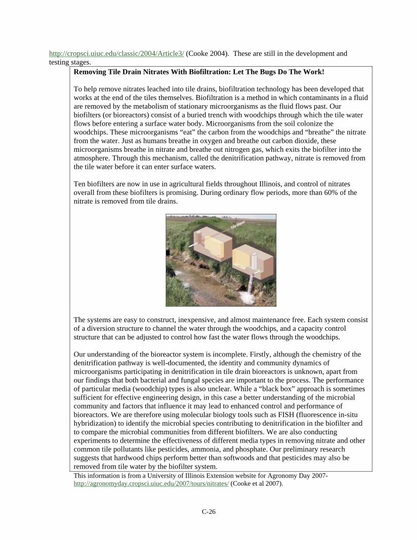
C-26
http://cropsci.uiuc.edu/classic/2004/Article3/ (Cooke 2004). These are still in the development and testing stages.
Removing Tile Drain Nitrates With Biofiltration: Let The Bugs Do The Work! To help remove nitrates leached into tile drains, biofiltration technology has been developed that works at the end of the tiles themselves. Biofiltration is a method in which contaminants in a fluid are removed by the metabolism of stationary microorganisms as the fluid flows past. Our biofilters (or bioreactors) consist of a buried trench with woodchips through which the tile water flows before entering a surface water body. Microorganisms from the soil colonize the woodchips. These microorganisms “eat” the carbon from the woodchips and “breathe” the nitrate from the water. Just as humans breathe in oxygen and breathe out carbon dioxide, these microorganisms breathe in nitrate and breathe out nitrogen gas, which exits the biofilter into the atmosphere. Through this mechanism, called the denitrification pathway, nitrate is removed from the tile water before it can enter surface waters. Ten biofilters are now in use in agricultural fields throughout Illinois, and control of nitrates overall from these biofilters is promising. During ordinary flow periods, more than 60% of the nitrate is removed from tile drains.
The systems are easy to construct, inexpensive, and almost maintenance free. Each system consist of a diversion structure to channel the water through the woodchips, and a capacity control structure that can be adjusted to control how fast the water flows through the woodchips. Our understanding of the bioreactor system is incomplete. Firstly, although the chemistry of the denitrification pathway is well-documented, the identity and community dynamics of microorganisms participating in denitrification in tile drain bioreactors is unknown, apart from our findings that both bacterial and fungal species are important to the process. The performance of particular media (woodchip) types is also unclear. While a “black box” approach is sometimes sufficient for effective engineering design, in this case a better understanding of the microbial community and factors that influence it may lead to enhanced control and performance of bioreactors. We are therefore using molecular biology tools such as FISH (fluorescence in-situ hybridization) to identify the microbial species contributing to denitrification in the biofilter and to compare the microbial communities from different biofilters. We are also conducting experiments to determine the effectiveness of different media types in removing nitrate and other common tile pollutants like pesticides, ammonia, and phosphate. Our preliminary research suggests that hardwood chips perform better than softwoods and that pesticides may also be removed from tile water by the biofilter system. This information is from a University of Illinois Extension website for Agronomy Day 2007- http://agronomyday.cropsci.uiuc.edu/2007/tours/nitrates/ (Cooke et al 2007).

C-27
References Bundy, L. G. 1986. Review- Timing Nitrogen Applications to Maximize Fertilizer Efficiency and Crop
Response in Conventional Corn Production. J. Fertilizer Issues 3: 99-106. Cooke, Richard. 2004. Developments in Agricultural Drainage in Illinois. Crop Sciences Website,
University of Illinois at Urbana-Champaign. http://cropsci.uiuc.edu/classic/2004/Article3/ Cooke, Richard, Malia Appleford and Paul Davidson. 2007. Removing Tile Drain Nitrates With
Biofiltration: Let The Bugs Do The Work! Agronomy Day 2007 Website, University of Illinois Extension. http://agronomyday.cropsci.uiuc.edu/2007/tours/nitrates/
Creamean, Jill. 2003. Water Quality Improvements with Drainage Management. NRCS Illinois
Success Story. http://www.il.nrcs.usda.gov/features/success/wqimprv-dm.html Illinois Department of Agriculture. Cost-share Funds Targeted to TMDL Watersheds.
http://www.agr.state.il.us/Environment/LandWater/tmdl.html Illinois Environmental Protection Agency, Bureau of Water, Watershed Management Section, Planning
Unit. TMDL Website, www.epa.state.il.us/water/tmdl Illinois Environmental Protection Agency. January 2004. Surface Discharging Private Sewage Disposal
Systems and Their Effects on Communities in Illinois. Bureau of Water, Springfield, IL. Frankenberger, Jane, Eileen Kladivko, Gary Sands, Dan Jaynes, Norm Fausey, Matt Helmers, Richard
Cooke, Jeff Strock, Kelly Nelson and Larry Brown. August 2006. Drainage Water Management for the Midwest. Purdue Extension. http://www.ces.purdue.edu/extmedia/WQ/WQ-44.pdf
Joint Committee on Administrative Rules 35 Ill. Adm. Code, Title 35: Environmental Protection.
http://www.ilga.gov/commission/jcar/admincode/035/035parts.html Lucas, Leanne, 2004, Surface Septic Systems in Illinois Failing- Dumping Raw Sewage, ACES News,
College of Aces, University of Illinois. http://www.aces.uiuc.edu/news/stories/news2956.html Meals, Donald W. and David C. Braun. March 2005. Methods to Reduce Indicator Bacteria Levels in
Agricultural Runoff in the Lake Champlain Basin. Lake Champlain Basin Program Techinical Report 50. Grand Isle, Vermont. http://www.lcbp.org .
National Environmental Services Center. Viewed September 2006. Septic System Information.
http://www.nesc.wvu.edu/nsfc_septicnews.htm . National Small Flows Clearinghouse. National Soil Survey Center. 2008. Personal communication with Steve Peaslee. Lincoln, Nebraska. National Resources Conservation Services (NRCS). September 2004. Illinois Drainage Water
Management Tour Brochure. USDA. http://www.spipipe.com/PDF/DWMTourBrochure.pdf

C-28
The Ohio State University. Viewed September 2006. Septic System Maintance. http://ohioline.osu.edu/aex-fact/0740.html . Ohio State University Extension Factsheet.
Power, J.F., Richard Wiese and Dale Flowerday. 2000. Managing Nitrogen for Water Quality- Lessons
from Management Systems Evaluation Area. Journal of Environmental Quality v29, n2, 355-366.
United States Department of Agriculture. Environmental Quality Incentives Program.
http://www.nrcs.usda.gov/programs/eqip/ United States Department of Commerce. September 1997. American Housing Survey for the United
States-1995. US Census Bureau. United States Environmental Protection Agency. EPA 832-K-05-002. January 2005. Decentralized
Wastewater Treatment Systems: A Program Study. http://www.epa.gov/owm/septic/pubs/septic_program_strategy.pdf
United States Environmental Protection Agency. EPA 833-R-04-001. August 2004. Report to Congress:
Impacts and Control of CSOs and SSOs. Office of Water, Washington D.C. http://cfpub.epa.gov/npdes/cso/cpolicy_report2004.cfm
Weinzierl, Rick, Patrick Weicherding, Brenda Cude, David Williams and Doug Peterson. 1996. 60 Ways
Farmers Can Protect Surface Water. North Central Extension Publication 589. University of Illinois Extension, Urbana, IL http://www.thisland.uiuc.edu/60ways/60ways.html.