verifying and discovering bbp-type formulas …jgreene/masters_reports/bbp paper fi… · ·...
TRANSCRIPT

VERIFYING AND DISCOVERING BBP-TYPE FORMULAS
Submitted by
Melissa Larson
Applied and Computational Mathematics
In partial fulfillment of the requirements
For the Degree of Master of Science
University of Minnesota Duluth
Duluth, MN
Spring 2008

2
Chapter 1: Introduction
There are numerous well-known formulas for , including
r
C
2 (where C=circumference and r=radius),
2 2 2 2 2 2 2
1 1 1 1 1lim 4
6 1 2nn
n n n n n n
from [8, p. 152],
2
2
2
2
2
2
4 11
32
52
72
92
112
2
from [6, p. 127 formula 14],
and
1
2
2 1
6 k k
from [2, p. 225 formula 16.27].
Another notable formula is
(1.1)
0 68
1
58
1
48
2
18
4
16
1
kk kkkk
,
credited to David Bailey, Peter Borwein, and Simon Plouffe in 1995 It is often called the
BBP-formula. They wrote “On the Rapid Computation of Various Polylogarithmic
Constants”, in which the formula was first mentioned, [5, p. 1].
The formula is significant as it permits the computation of the nth hexadecimal digit
of without calculation the preceding 1n digits. The algorithm is explained in [5,

3
section 3 p.6-8], [2, p.129], and [4, p.123]. Since its discovery, formulas of similar form have
been discovered and have become known as BBP-type formulas. The general BBP-type
formula has the form
0 )(
)(
kk kqb
kp ,
where is a constant, p and q are polynomials with integer coefficients, deg( ) deg( )p q ,
( ) / ( )p k q k is nonsingular for nonnegative k , and b is an integer, [3, p. 2].
Many nice BBP-type formulas can be written
1 2
0 1 2
nk n
k
aa ax
nk nk nk n
,
where is a well-known constant, naaa ,,, 21 are constants (usually integers), and
1nxb
. We call n the base of the BBP form. This is the only form I considered in this
project.
A few examples of BBP-type formulas are the following:
0
11
2 1 4
k
k k
,
which is known as the Leibniz formula,
1
1 1ln 2
2
k
k k
,
and
4
0 78
1
58
2
38
4
18
8
16
1
2
1arctan28
kk kkkk
from [5, p. 6].
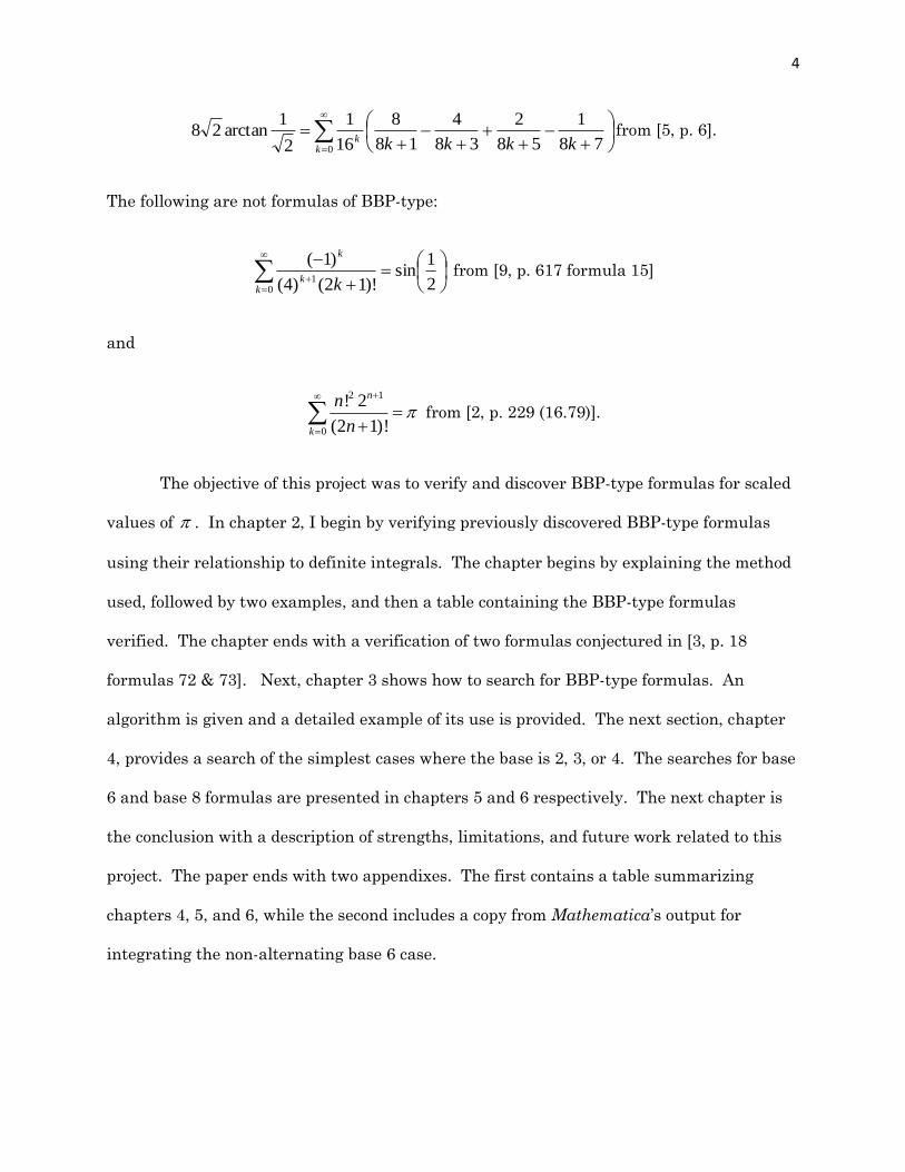
The following are not formulas of BBP-type:
2
1sin
)!12()4(
)1(
01
kk
k
k from [9, p. 617 formula 15]
and
2 1
0
! 2
(2 1)!
n
k
n
n
from [2, p. 229 (16.79)].
The objective of this project was to verify and discover BBP-type formulas for scaled
values of . In chapter 2, I begin by verifying previously discovered BBP-type formulas
using their relationship to definite integrals. The chapter begins by explaining the method
used, followed by two examples, and then a table containing the BBP-type formulas
verified. The chapter ends with a verification of two formulas conjectured in [3, p. 18
formulas 72 & 73]. Next, chapter 3 shows how to search for BBP-type formulas. An
algorithm is given and a detailed example of its use is provided. The next section, chapter
4, provides a search of the simplest cases where the base is 2, 3, or 4. The searches for base
6 and base 8 formulas are presented in chapters 5 and 6 respectively. The next chapter is
the conclusion with a description of strengths, limitations, and future work related to this
project. The paper ends with two appendixes. The first contains a table summarizing
chapters 4, 5, and 6, while the second includes a copy from Mathematica’s output for
integrating the non-alternating base 6 case.

5
Chapter 2: Unified Method to Verify
A technique was used to verify various BBP-type formulas. This chapter will
provide a detail explanation of the technique’s steps. Also provided is a table of formulas
from the literature I have verified by this method.
Recall, in this project, I am interested in formulas of the type
1 2
0 1 2
nk n
k
aa ax
nk nk nk n
,
where is a well-known constant, 1 2, , , na a a are constants (usually integers), and x is a
constant. The key formulas are presented in Theorem 1 and Theorem 2.
Theorem 1: If 0 1x or if 1x and 01
n
i
ia , then
11
1 21 2
00 1 2 1
nnk n n
n nk
a a a u a ua ax du
nk nk nk n x u
.
Proof: The series is a power series with radius of convergence 1. If 1x , we can
integrate and differentiate as stated in [1, p. 173 Theorem 6.5.7]. When 1x and
01
n
i
ia , the resulting sum will converge by the limit comparison test with
2
1
1k .
We only verify the case when 1x below.
Let
1 2
0 1 2
nk n
k
aa ax
nk nk nk n
.

6
We break this into n summations,
1 2
0 0 01 2
nknk nk
n
k k k
a xa x a x
nk nk nk n
.
Taking each term individually, let 11
0
( )1
nk
k
a xf x
nk
. Multiplying both sides by x
gives
1
11
0
( )1
nk
k
a xx f x
nk
. By taking the derivative we get,
1 1
1 1
1
0 0
( ) 1
1
nk
nk
k k
d x f x a nk xa x
dx nk
.
This is a geometric series which can be summed, 1 1
( )
1 n
d x f x a
dx x
. By the Fundamental
Theorem of Calculus, 11
0( )
1
x
n
ax f x dt
t
, which implies 11
0
1( )
1
x
n
af x dt
x t
when 0x .
Similarly, for the thi summation, let
0
( )nk
ii
k
a xf x
nk i
. As before
1
0 0
( )i nk ii nk ii
i
k k
d x f x a xda x
dx dx nk i
,
a geometric series that sums to
1
1
i
i
n
a x
x
. Integrating gives
1
0( )
1
ix
i ii n
a tx f x dt
t
. Thus,
1
0
1( )
1
i
ix
i n
ta
xf x dt
x t
.
Adding the n terms,

7
1
1 2
1 2
00 0 0
1
1 2 1
n
nknk nk nx
n
nk k k
t ta a a
a xa x a x x xdt
nk nk nk n x t
.
Finally, using the substitution x
tu we obtain
11
1 2
0 1
n
n
n n
a a u a udu
x u
. ■
Therefore, verifying
1 2
0 1 2
nk n
k
aa ax
nk nk nk n
is equivalent to verifying
11
1 2
0 1
n
n
n n
a a u a udu
x u
.
We were also interested in the alternating case of the form,
1 2
0 1 2
kn n
k
aa ax
nk nk nk n
.
We have:
Theorem 2: If 0 1x or 1x , then
1
11 21 2
00 1 2 1
nk
n n n
n nk
a a a u a ua ax du
nk nk nk n x u
.
Proof: Again, we only give a proof in the case where 0 1x .
8
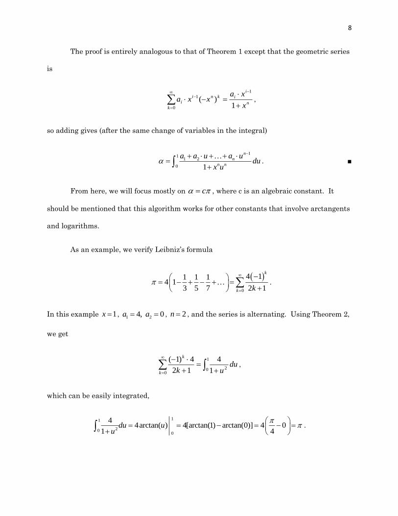
The proof is entirely analogous to that of Theorem 1 except that the geometric series
is
0
1
1
1)(
kn
i
ikni
ix
xaxxa ,
so adding gives (after the same change of variables in the integral)
11
1 2
0 1
n
n
n n
a a u a udu
x u
. ■
From here, we will focus mostly on c , where c is an algebraic constant. It
should be mentioned that this algorithm works for other constants that involve arctangents
and logarithms.
As an example, we verify Leibniz’s formula
0
4 11 1 14 1
3 5 7 2 1
k
k k
.
In this example 1x , 1 24, 0a a , 2n , and the series is alternating. Using Theorem 2,
we get
0
1
0 21
4
12
4)1(
k
k
duuk
,
which can be easily integrated,
11
200
44arctan( ) 4[arctan(1) arctan(0)] 4 0
1 4du u
u
.

9
This verifies
0
4 1
2 1
k
k k
.
The original BBP formula is
0 68
1
58
1
48
2
18
4
16
1
kk kkkk
.
Here 1
2x , 1 4 5 6 2 3 7 84, 2, 1, 1, 0a a a a a a a a , 8n , and it is non-
alternating. To verify this formula is equivalent to verifying that
3 4 51
80
4 2
116
u u udu
u
,
by Theorem 1. Factoring the numerator and denominator, we cancel out common terms,
3 4 5 4 3 21 1
8 4 3 4 3 20 0
1
4 30
4 2 (16 16)( 2 4 4 4)
( 2 4 4)( 2 4 4 4)1
16
16 16.
2 4 4
u u u u u u u udu du
u u u u u u u u
udu
u u u
Using partial fractions, we get
1 1
4 3 2 20 0
16 16 4 4( 2)
2 4 4 2 2 2
u u udu du
u u u u u u
,
two quadratic terms which can be integrated by hand. We have

10
1 1 0
2 2 20 2 1
12 2
0
4 4( 2) 2 4 4
2 2 2 1
2ln 2 2ln ( 1) 1 4arctan( 1)
2ln 2 2ln 2
.
u u vdu dw dv
u u u w v
u u u
As in the previous example, when verifying BBP-type formulas it is common that the
rational polynomial’s numerator and denominator will have common factors that cancel
out. Also, the remaining rational polynomial usually has a nice partial fractions
decomposition.
For convenience, we use the notation
1 21 2
0
11
1 2
0
( , , ( , , , ))1 2
1
nk nn
k
n
n
n n
aa aBPP x n a a a x
nk nk nk n
a a u a udu
x u
and
1 21 2
0
11
1 2
0
( , , ( , , , ))1 2
.1
kn n
n
k
n
n
n n
aa aABPP x n a a a x
nk nk nk n
a a u a udu
x u
The following tables contain BBP-type formulas from the literature which I have
verified.

11
Table 1- BBP-type formulas verified for the bases 4, 6, and 8.
BBP -Type Formula Partial Fractions Breakdown
1
, 4, (2, 2, 1, 0)2
ABBP a
2
4
2 2u u
32 3
9
1, 6, (16, 8, 0, 2, 1, 0)
2BBP
a
2
64
2 4u u
32 3
9
1, 6, (0, 32, 8, 4, 2, 0)
2BBP
c
2 2
160 32 128( 1) 64( 2)
3( 2) 3(2 ) 3( 2 4) 3( 2 4)
u u
u u u u u u
4 3 1
, 6, (20, 6, 1, 3, 1, 0)2
BBP b
42
)10(8
2
4
2
42
uu
u
uu
1
, 8, (4, 0, 0, 2, 1, 1, 0, 0)2
BBP b
2 2
4 4( 2)
2 2 2
u u
u u u
2 1
, 8, (0, 8, 4, 4, 0, 0, 1, 0)2
BBP
b
22
8
2
822
uu
u
u
u
a-These formulas came from [3, p. 5 formula 6 and p.7 formula 16].
b-These formulas came from [11, formulas 11, 2, and 3].
c-This formula comes from a combination of formulas from [3, p.7 formula 16 minus p.16
formula 59].
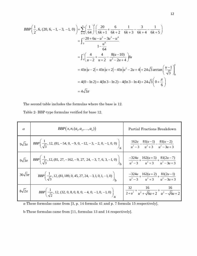
For example, for the fourth row,
12
0
2 3 41
60
1
20
1
2
0
1 1 20 6 1 3 1, 6, (20, 6, 1, 3, 1, 0)
2 64 6 1 6 2 6 3 6 4 6 5
20 6 3
164
4 4 8( 10)
2 2 2 4
14ln 2 4ln 2 4ln 2 4 24 3 arctan
3
4(0 ln 2)
k
k
BBPk k k k k
u u u u
u
udu
u u u u
uu u u u
4(ln3 ln 2) 4(ln3 ln 4) 24 3 06
4 3
The second table includes the formulas where the base is 12.
Table 2- BBP-type formulas verified for base 12.
1 2, , ( , , , )nBBP x n a a a Partial Fractions Breakdown
9 3 1
, 12, (81, 54, 0, 9, 0, 12, 3, 2, 0, 1, 0, 0)3
BBP a
2 2 2
162 81( 1) 81( 2)
3 3 3 3
u u u
u u u u
9 3 1
,12, (81, 27, 162, 9, 27, 24, 3, 7, 6, 3, 1, 0)3
BBP b
2 2 2
324 162( 5) 81(2 7)
3 3 3 3
u u u
u u u u
36 3
1,12, (81,189, 0, 45, 27, 24, 3,1, 0,1, 1, 0)
3BBP
b
2 2 2
324 162( 2) 81(2 1)
3 3 3 3
u u u
u u u u
8 2
1, 12, (32, 0, 8, 0, 8, 0, 4, 0, 1, 0, 1, 0)
2BBP
a
2 2 2
32
2
16 16
6 2 6 2u u u u u
a-These formulas came from [3, p. 14 formula 41 and p. 7 formula 15 respectively].
b-These formulas came from [11, formulas 13 and 14 respectively].
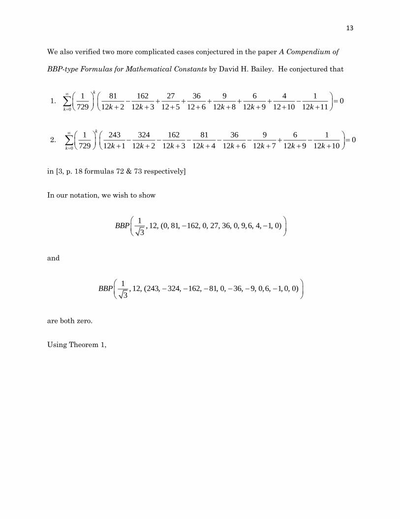
13
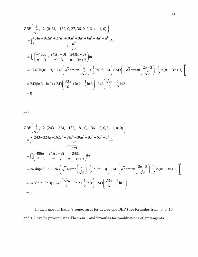
We also verified two more complicated cases conjectured in the paper A Compendium of
BBP-type Formulas for Mathematical Constants by David H. Bailey. He conjectured that
1. 0
1 81 162 27 36 9 6 4 10
729 12 2 12 3 12 5 12 6 12 8 12 9 12 10 12 11
k
k k k k k k
2. 0
1 243 324 162 81 36 9 6 10
729 12 1 12 2 12 3 12 4 12 6 12 7 12 9 12 10
k
k k k k k k k k k
in [3, p. 18 formulas 72 & 73 respectively]
In our notation, we wish to show
1, 12, (0, 81, 162, 0, 27, 36, 0, 9,6, 4, 1, 0)
3BBP
and
1, 12, (243, 324, 162, 81, 0, 36, 9, 0,6, 1, 0, 0)
3BBP
are both zero.
Using Theorem 1,
14
2 4 5 7 8 9 101
120
1
2 2 20
2 2
1, 12, (0, 81, 162, 0, 27, 36, 0, 9,6, 4, 1, 0)
3
81 162 27 36 9 6 4
1729
486 243( 3) 243( 3)
3 3 3 3
1243ln( 3) 243 3 arctan ln( 3) 243
23
BBP
u u u u u u u udu
u
u u udu
u u u u
uu u
1
2
0
2 3 13 arctan ln( 3 3)
23
3 1 3 1243(ln3 ln 2) 243 ln 2 ln3 243 ln3
6 2 6 2
0
uu u
and
2 3 5 6 8 91
120
1
2 2 20
2 2
1, 12, (243, 324, 162, 81, 0, 36, 9, 0,6, 1, 0, 0)
3
243 324 162 81 36 9 6
1729
486 243( 3) 243
3 3 3 3
1243ln( 3) 243 3 arctan ln( 3) 243
23
BBP
u u u u u u udu
u
u u udu
u u u u
uu u
1
2
0
2 3 13 arctan ln( 3 3)
23
3 1 3 1243(ln 2 ln3) 243 ln 2 ln3 243 ln3
6 2 6 2
0.
uu u
In fact, most of Bailey’s conjectures for degree one BBP-type formulas from [3, p. 16
and 18] can be proven using Theorem 1 and formulas for combinations of arctangents.
15
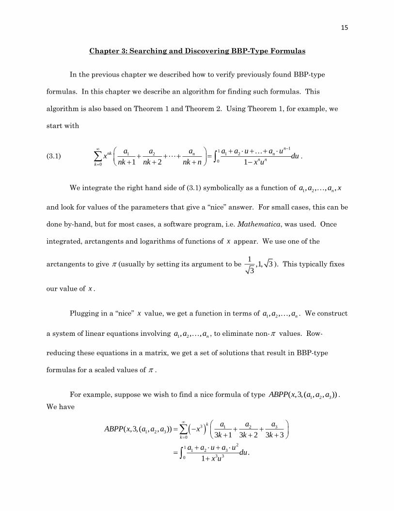
Chapter 3: Searching and Discovering BBP-Type Formulas
In the previous chapter we described how to verify previously found BBP-type
formulas. In this chapter we describe an algorithm for finding such formulas. This
algorithm is also based on Theorem 1 and Theorem 2. Using Theorem 1, for example, we
start with
(3.1)
11
1 21 2
00 1 2 1
nnk n n
n nk
a a a u a ua ax du
nk nk nk n x u
.
We integrate the right hand side of (3.1) symbolically as a function of 1 2, , , ,na a a x
and look for values of the parameters that give a “nice” answer. For small cases, this can be
done by-hand, but for most cases, a software program, i.e. Mathematica, was used. Once
integrated, arctangents and logarithms of functions of x appear. We use one of the
arctangents to give (usually by setting its argument to be 1
,1, 33
). This typically fixes
our value of x .
Plugging in a “nice” x value, we get a function in terms of 1 2, , , na a a . We construct
a system of linear equations involving 1 2, , , na a a , to eliminate non- values. Row-
reducing these equations in a matrix, we get a set of solutions that result in BBP-type
formulas for a scaled values of .
For example, suppose we wish to find a nice formula of type 1 2 3( ,3,( , , ))ABPP x a a a .
We have
3 31 21 2 3
0
21
1 2 3
3 30
( ,3, ( , , ))3 1 3 2 3 3
.1
k
k
aa aABPP x a a a x
k k k
a a u a udu
x u

16
from Theorem 2. Using Mathematica to perform the integral,
1 21 2 3 1 222
2 2 2
1 2 3 1 2 3
( ) 1 1 2( ,3, ( , , )) 2 3 ( )arctan
66 3 3
2( 2 ) ln(1 ) ( 2 ) ln(1 ) .
a x a xABPP x a a a x a x a
xx
a x a x a x a x a x a x x
We can get an expression involving using either 1 2
2
( )
6 3
a x a
x
or
1 2arctan
3
x
. When
using 1 2
2
( )
6 3
a x a
x
, we need to eliminate other terms. The arctangent term can only be
eliminated by setting 1
2x , (since we cannot use 1 2( )a x a or our value would be
eliminated also). We have
1 2 3 1 2 1 2 3 3
1 1,3,( , , ) 3 2 3 3 6 48 ln3 72 ln 2
2 9ABPP a a a a a a a a a
.
Thus, we need 1 2 33 6 48 0a a a and 372 0a . Row reducing
3 6 48 0
0 0 72 0
we get
1 2 0 0
0 0 1 0
,
implying 1 22a a and 3 0a , resulting in the BBP-type formula
(3.2) 0
1 1 2 1 4 3,3,(2,1,0)
2 8 3 1 3 2 9
k
k
ABBPk k
.
Alternatively, when 1x ,
17
63
1arctan
3
21arctan
x.
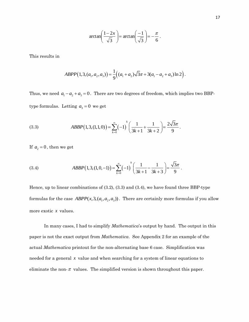
This results in
1 2 3 1 2 1 2 3
11,3,( , , ) ( ) 3 3( ) ln 2
9ABPP a a a a a a a a .
Thus, we need 1 2 3 0a a a . There are two degrees of freedom, which implies two BBP-
type formulas. Letting 3 0a we get
(3.3) 0
1 1 2 31,3,(1,1,0) 1
3 1 3 2 9
k
k
ABBPk k
.
If 2 0a , then we get
(3.4) 0
1 1 31,3,(1,0, 1) 1
3 1 3 3 9
k
k
ABBPk k
.
Hence, up to linear combinations of (3.2), (3.3) and (3.4), we have found three BBP-type
formulas for the case 1 2 3( ,3,( , , ))ABPP x a a a . There are certainly more formulas if you allow
more exotic x values.
In many cases, I had to simplify Mathematica’s output by hand. The output in this
paper is not the exact output from Mathematica. See Appendix 2 for an example of the
actual Mathematica printout for the non-alternating base 6 case. Simplification was
needed for a general x value and when searching for a system of linear equations to
eliminate the non- values. The simplified version is shown throughout this paper.

18
Chapter 4: Examining Cases Where the Base is 2, 3, or 4
Using the algorithm described in the last section, we searched for BBP-type
formulas for non-alternating and alternating bases 2, 3, 4, 6, and 8. In this chapter, we
present the results for the simplest cases, bases 2, 3, and 4. The simplest case of all is the
alternating base 2 case.
From Theorem 2 we have
2 1 21 2
0
11 2
2 20
, 2, ( , )2 1 2 2
.1
k
k
a aABBP x a a x
k k
a a udu
x u
After integrating, we get
2
1 2 1 22
1, 2, ( , ) 2 arctan( ) ln(1 )
2ABBP x a a a x x a x
x .
From this equation we look for “nice” x -values. The criteria for x to be “nice” are
that nx needs to be rational and its use allows for the evaluate or eliminate an arctangent.
In order to eliminate an arctangent, we need to be a result of the integral which does not
always occur.
In the above example, the two values 1
3x or 1x lead to interesting formulas
since 63
1arctan
and
41arctan
. When
1
3x ,
1 21 2
31 4, 2, ( , ) ln
2 33 2 3
a aABBP a a
.

19
Thus 2 0a , which results in the BBP-type formula
(4.1) 0
1 1 1 3, 2, (1, 0)
3 2 1 63
k
k
ABBPk
.
When 1x ,
21 2 11, 2, ( , ) ln(2)
4 2
aABBP a a a
.
Thus 2 0a , which gives
(4.2) 0
11, 2, (1, 0) 1
2 1 4
k
k
ABBPk
,
the Leibniz formula again.
For non-alternating formulas with base 3n , from Theorem 1, we have
3 31 21 2 3
0
21
1 2 3
3 30
( ,3, ( , , ))3 1 3 2 3 3
.1
k
k
aa aBPP x a a a x
k k k
a a u a udu
x u
Using Mathematica to integrate,
2 2
1 2 3 1 2 3 1 23
2 2 2 2
1 2 1 2 3 1 2 3
1( ,3, ( , , )) ( )6 ( ) 3
18
1 26 3( )arctan 6( ) ln( 1) 3( 2 ) ln( 1) .
3
BPP x a a a a x a x a i a x a xx
xa x a x a x a x a x a x a x a x x

20
The only “nice” x value appears to be 1x since we then have 3
3arctan
. With 1x
we have
1 2 3 1 2 3 1 2 1 2
1(1,3,( , , )) ( )6 ( ) 3 3( ) ln3
18BPP a a a a a a i a a a a .
This implies that 1 2 3 0a a a and 1 2 0a a . Row-reducing
1 1 1 0
1 1 0 0
yields
1 1 0 0
0 0 1 0
.
Thus, 1 2a a and 3 0a , resulting in the BBP-type formula
(4.3) 0
1 1 3(1,3, (1, 1,0))
3 1 3 2 9k
BPPk k
.
The alternating base 3 formulas were investigated in the previous chapter.
Next we will examine non-alternating base 4 formulas,
2 3
11 2 3 4
1 2 3 4 4 40, 4, ( , , , )
1
a a u a u a uBBP x a a a a du
x u
.
Using Mathematica,
21
3 2 3
1 2 3 4 2 3 4 1 32 1
3 2 3 2 2 2
1 2 3 4 1 2 3 4 2 4
1, 4, ( , , , ) ( ) 2( )arctan( )
4
( ) ln( 1) ( ) ln( 1) ( ) ln( 1) .
BBP x a a a a a x a x a x a i a x a x xx
a x a x a x a x a x a x a x a x a x a x
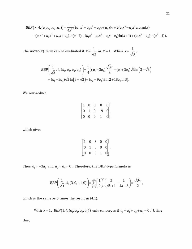
The )arctan(x term can be evaluated if 1
3x or 1x . When
1
3x ,
1 2 3 4 1 3 1 3
1 3 2 4 4
1 1 3, 4, ( , , , ) ( 3 ) ( 3 ) 3 ln 3 3
4 33
( 3 ) 3 ln 3 3 ( 9 )3ln 2 18 ln3 .
BBP a a a a a a a a
a a a a a
We row-reduce
1 0 3 0 0
0 1 0 9 0
0 0 0 1 0
,
which gives
1 0 3 0 0
0 1 0 0 0
0 0 0 1 0
.
Thus 1 33a a and 2 4 0a a . Therefore, the BBP-type formula is
0
1 1 3 1 3, 4, (3, 0, 1, 0)
9 4 1 4 3 23
k
k
BBPk k
,
which is the same as 3 times the result in (4.1).
With 1x , 1 2 3 41, 4, ( , , , )BBP a a a a only converges if 1 2 3 4 0a a a a . Using
this,
22
1 2 3 4 1 3 1 3 4
11, 4, ( , , , ) ( ) ( 2 ) ln 2 .
4 2BBP a a a a a a a a a
Hence, we row-reduce
1 1 1 1 0
1 0 1 2 0
and get
1 0 1 2 0
0 1 0 3 0
.
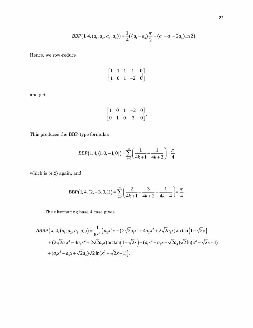
This produces the BBP-type formulas
0
1 11, 4, (1, 0, 1, 0)
4 1 4 3 4k
BBPk k
which is (4.2) again, and
0
2 3 11, 4, (2, 3, 0,1)
4 1 4 2 4 4 4k
BBPk k k
.
The alternating base 4 case gives
2 3 2
1 2 3 4 2 1 2 34
3 2 3 2
1 2 3 1 3 4
3 2
1 3 4
1, 4, ( , , , ) ( 2 2 4 2 2 )arctan 1 2
8
(2 2 4 2 2 )arctan 1 2 ( 2 ) 2 ln( 2 1)
( 2 ) 2 ln( 2 1) .
ABBP x a a a a a x a x a x a x xx
a x a x a x x a x a x a x x
a x a x a x x
23
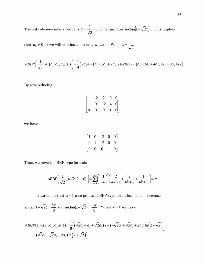
The only obvious nice x value is 1
2x which eliminates x21arctan . This implies
that 02 a or we will eliminate our only term. When 1
2x
1 2 3 4 2 1 2 3 1 3 4 4
1 1, 4, ( , , , ) 2 ( 2 2 )2arctan 2 ( 2 4 ) ln5 8 ln 2 .
42ABBP a a a a a a a a a a a a
By row-reducing
1 2 2 0 0
1 0 2 4 0
0 0 0 1 0
we have
1 0 2 0 0
0 1 2 0 0
0 0 0 1 0
.
Thus, we have the BBP-type formula
0
1 1 2 2 1, 4, (2, 2,1, 0)
4 4 1 4 2 4 32
k
k
ABBPk k k
.
It turns out that 1x also produces BBP-type formulas. This is because
3arctan(1 2)
8
and arctan(1 2)
8
. When 1x we have
1 2 3 4 1 2 3 1 3 4
1 3 4
11,4, ( , , , ) ( 2 2 ) ( 2 2 2 ) ln 2 2
8
( 2 2 2 ) ln 2 2 .
ABBP a a a a a a a a a a
a a a
.
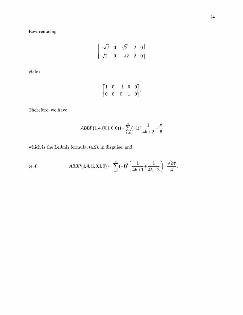
24
Row-reducing
2 0 2 2 0
2 0 2 2 0
yields
1 0 1 0 0
0 0 0 1 0
.
Therefore, we have
0
11,4,(0,1,0,0) ( 1)
4 2 8
k
k
ABBPk
which is the Leibniz formula, (4.2), in disguise, and
(4.4) 0
1 1 21,4,(1,0,1,0) ( 1)
4 1 4 3 4
k
k
ABBPk k
.
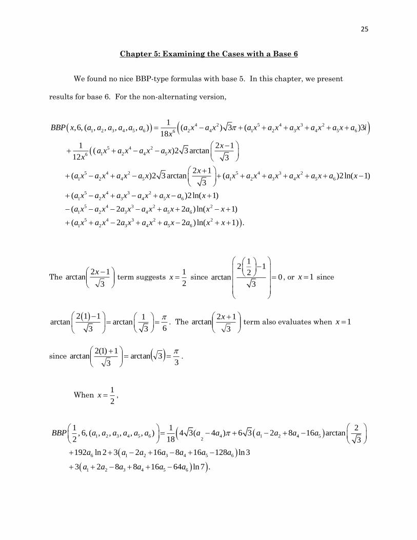
25
Chapter 5: Examining the Cases with a Base 6
We found no nice BBP-type formulas with base 5. In this chapter, we present
results for base 6. For the non-alternating version,
4 2 5 4 3 2
1 2 3 4 5 6 2 4 1 2 3 4 5 66
5 4 2
1 2 4 56
5 4 2 5 4 3 2
1 2 4 5 1 2 3 4 5 6
1,6, ( , , , , , ) ( ) 3 ( )3
18
1 2 1( )2 3 arctan
12 3
2 1( )2 3 arctan ( )2ln( 1)
3
(
BBP x a a a a a a a x a x a x a x a x a x a x a ix
xa x a x a x a x
x
xa x a x a x a x a x a x a x a x a x a x
5 4 3 2
1 2 3 4 5 6
5 4 3 2 2
1 2 3 4 5 6
5 4 3 2 2
1 2 3 4 5 6
)2ln( 1)
( 2 2 ) ln( 1)
( 2 2 ) ln( 1) .
a x a x a x a x a x a x
a x a x a x a x a x a x x
a x a x a x a x a x a x x
The
3
12arctan
x term suggests
1
2x since
12 1
2arctan 0
3
, or 1x since
2 1 1 1arctan arctan
63 3
. The
3
12arctan
x term also evaluates when 1x
since 3
3arctan3
1)1(2arctan
.
When 1
2x ,
1 2 3 4 5 6 4 1 2 4 52
6 1 2 3 4 5 6
1 2 3 4 5 6
1 1 2, 6, ( , , , , , ) 4 3( 4 ) 6 3 2 8 16 arctan
2 18 3
192 ln 2 3 2 16 8 16 128 ln3
3 2 8 8 16 64 ln 7 .
BBP a a a a a a a a a a a a
a a a a a a a
a a a a a a

26
Row-reducing
1 2 0 8 16 0 0
0 0 0 0 0 192 0
1 2 16 8 16 128 0
1 2 8 8 16 64 0
we get
1 0 0 4 8 0 0
0 1 0 2 12 0 0
0 0 1 1 2 0 0
0 0 0 0 0 1 0
.
Thus,
0
1 1 4 2 1 1 4 3, 6, (4, 2, 1, 1, 0, 0)
2 64 6 1 6 2 6 3 6 4 9
k
k
BBPk k k k
and
0
1 1 8 12 2 1 8 3, 6, (8, 12, 2,0, 1, 0)
2 64 6 1 6 2 6 3 6 5 3
k
k
BBPk k k k
.
When 1x , we need 0654321 aaaaaa for convergence. Using this,
1 2 3 4 5 6 1 2 4 5
1 2 3 4 5 6 1 2 3 4 5 6
11, 6, ( , , , , , ) (3 3 ) 3
36
( )6ln 2 ( 2 2 )3ln3 .
BBP a a a a a a a a a a
a a a a a a a a a a a a
Row-reducing

27
0211211
0111111
0111111
yields
1 0 0 0 1 1 0
0 1 0 1 0 1 0
0 0 1 0 0 1 0
.
Thus, we have
0
1 1 31, 6, (1, 0, 0, 0, 1, 0)
6 1 6 5 6k
BBPk k
,
0
1 1 31, 6, (0,1, 0, 1, 0, 0)
6 2 6 4 18k
BBPk k
,
and
0
1 1 1 1 31, 6, (1, 1, 1, 0, 0, 1)
6 1 6 2 6 3 6 6 18k
BBPk k k k
.
The second of these is equivalent to the formula (4.3) for base 3.
In the alternating case, we have
2 5 3
1 2 3 4 5 6 2 4 1 3 56
5 4 3 2
1 2 3 4 5
5 4 3 2 4 2 2
1 2 3 4 5 2 4 6
5 4 2
1 2 4 5 6
1( , 6, ( , , , , , ) ( )2 3 ( )4arctan
12
( 3 2 3 )2arctan 3 2
( 3 2 3 )2arctan 3 2 ( )2ln 1
( 3 3 2 ) l
ABBP x a a a a a a a x a a x a x a x xx
a x a x a x a x a x x
a x a x a x a x a x x a x a x a x
a x a x a x a x a
2
5 4 2 2
1 2 4 5 6
n 3 1
( 3 3 2 ) ln 3 1 .
x x
a x a x a x a x a x x
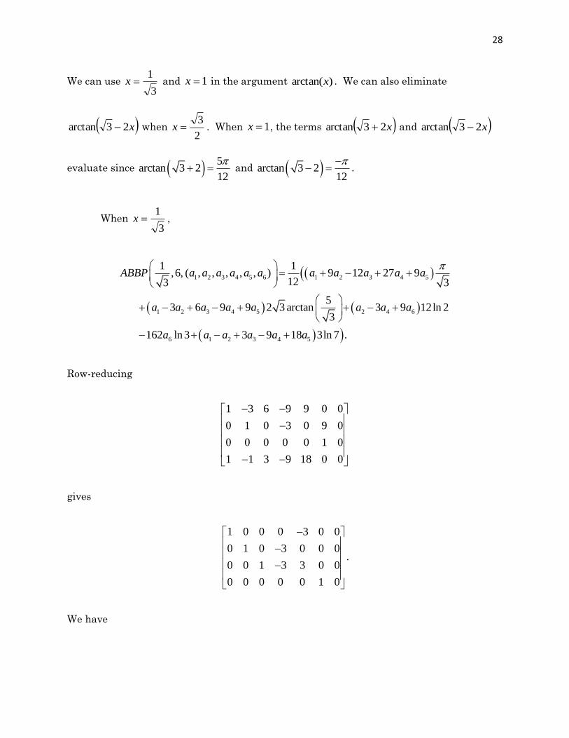
28
We can use 3
1x and 1x in the argument )arctan(x . We can also eliminate
x23arctan when 2
3x . When 1x , the terms x23arctan and x23arctan
evaluate since 5
arctan 3 212
and arctan 3 2
12
.
When 3
1x ,
1 2 3 4 5 6 1 2 3 4 5
1 2 3 4 5 2 4 6
6 1 2 3 4 5
1 1,6, ( , , , , , ) 9 12 27 9
123 3
53 6 9 9 2 3 arctan 3 9 12ln 2
3
162 ln3 3 9 18 3ln 7 .
ABBP a a a a a a a a a a a
a a a a a a a a
a a a a a a
Row-reducing
1 3 6 9 9 0 0
0 1 0 3 0 9 0
0 0 0 0 0 1 0
1 1 3 9 18 0 0
gives
1 0 0 0 3 0 0
0 1 0 3 0 0 0
0 0 1 3 3 0 0
0 0 0 0 0 1 0
.
We have
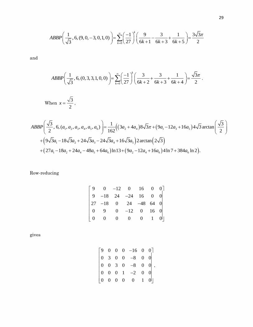
29
0
1 1 9 3 1 3 3, 6, (9, 0, 3, 0,1, 0)
27 6 1 6 3 6 5 23
k
k
ABBPk k k
and
0
1 1 3 3 1 3, 6, (0, 3, 3,1, 0, 0)
27 6 2 6 3 6 4 23
k
k
ABBPk k k
.
When 2
3x ,
1 2 3 4 5 6 2 4 1 3 5
1 2 3 4 5
1 2 4 5 6 2 4 6 6
3 1 3, 6, ( , , , , , ) 3 4 8 3 9 12 16 4 3 arctan
2 162 2
9 3 18 3 24 3 24 3 16 3 2arctan 2 3
27 18 24 48 64 ln13 9 12 16 4ln 7 384 ln 2 .
ABBP a a a a a a a a a a a
a a a a a
a a a a a a a a a
Row-reducing
9 0 12 0 16 0 0
9 18 24 24 16 0 0
27 18 0 24 48 64 0
0 9 0 12 0 16 0
0 0 0 0 0 1 0
gives
9 0 0 0 16 0 0
0 3 0 0 8 0 0
0 0 3 0 8 0 0
0 0 0 1 2 0 0
0 0 0 0 0 1 0
,
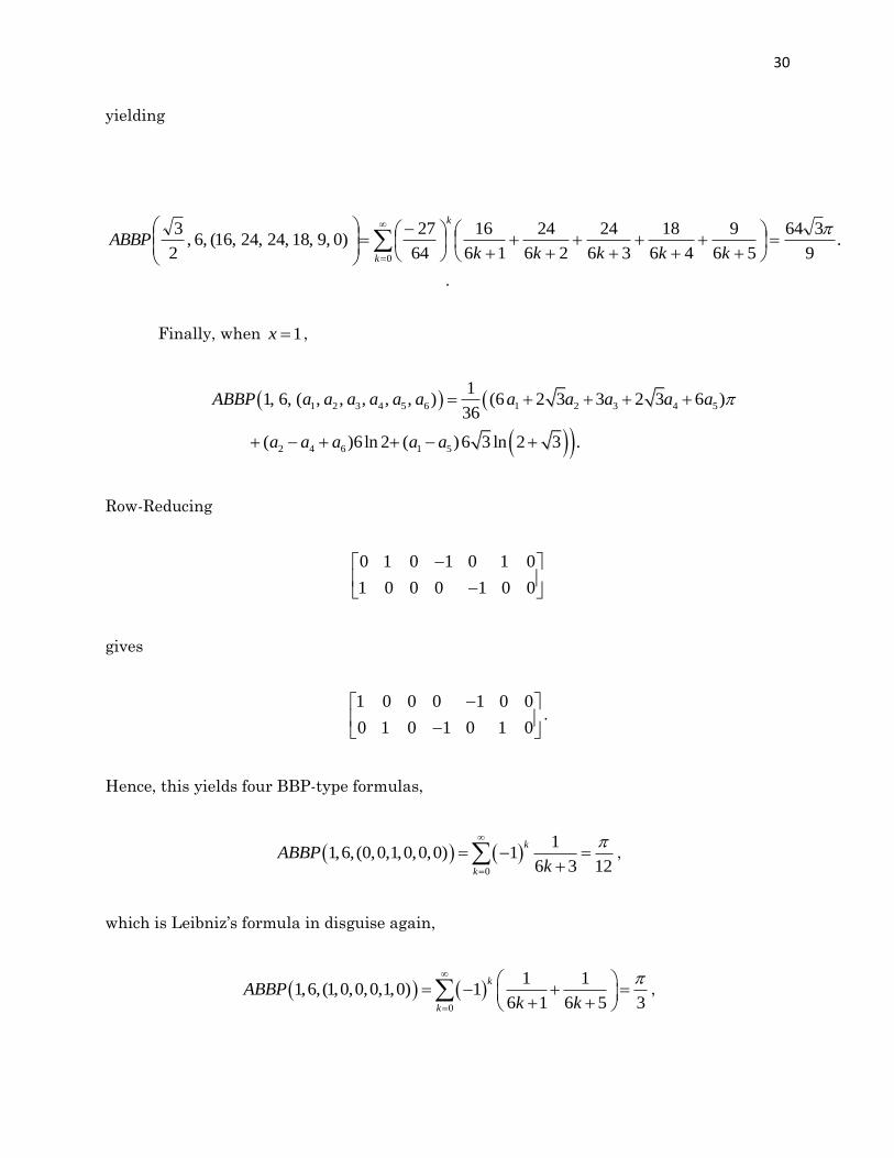
30
yielding
0
.9
364
56
9
46
18
36
24
26
24
16
16
64
27)0,9,18,24,24,16(,6,
2
3
k
k
kkkkkABBP
.
Finally, when 1x ,
1 2 3 4 5 6 1 2 3 4 5
2 4 6 1 5
11, 6, ( , , , , , ) (6 2 3 3 2 3 6 )
36
( )6ln 2 ( )6 3 ln 2 3 .
ABBP a a a a a a a a a a a
a a a a a
Row-Reducing
0 1 0 1 0 1 0
1 0 0 0 1 0 0
gives
1 0 0 0 1 0 0
0 1 0 1 0 1 0
.
Hence, this yields four BBP-type formulas,
0
11,6,(0,0,1,0,0,0) 1
6 3 12
k
k
ABBPk
,
which is Leibniz’s formula in disguise again,
0
1 11,6,(1,0,0,0,1,0) 1
6 1 6 5 3
k
k
ABBPk k
,
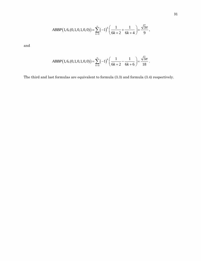
31
0
1 1 31,6,(0,1,0,1,0,0) 1
6 2 6 4 9
k
k
ABBPk k
,
and
0
1 1 31,6,(0,1,0,1,0,0) 1
6 2 6 6 18
k
k
ABBPk k
.
The third and last formulas are equivalent to formula (3.3) and formula (3.4) respectively.

32
Chapter 6: Examining Cases with Base 8
This chapter deals with BBP-type formulas with base 8. There do not appear to be
any “nice” formulas with base 7. In the non-alternating case,
.12ln2)22(
12ln2)22(
21arctan2)2222(
21arctan2)2222(
)1ln(2)()arctan(4)(
)1ln(2)(
)1ln(2)(2)(
2)(16
1),,,,,,,(,8,
2
87
3
5
4
4
5
3
7
1
2
87
3
5
4
4
5
3
7
1
7
2
6
3
5
5
3
6
2
7
1
7
2
6
3
5
5
3
6
2
7
1
2
8
2
6
4
4
6
27
3
5
5
3
7
1
87
2
6
3
5
4
4
5
3
6
2
7
1
87
2
6
3
5
4
4
5
3
6
2
7
1
2
6
6
2
87
2
6
3
5
4
4
5
3
6
2
7
1287654321
xxaxaxaxaxaxa
xxaxaxaxaxaxa
xxaxaxaxaxaxa
xxaxaxaxaxaxa
xaxaxaxaxxaxaxaxa
xaxaxaxaxaxaxaxa
xaxaxaxaxaxaxaxaxaxa
iaxaxaxaxaxaxaxax
aaaaaaaaxBBP
Possible x -values are 3
1x and 1x from )arctan(x . We can also eliminate
)21arctan( x if 2
1x . The term )21arctan( x also evaluates when x=1 since
3arctan(1 2)
8
and arctan(1 2)
8
.
When 3
1x ,
1 2 3 4 5 6 7 8 1 2 3 5 6 7
1 2 3 5 6 7
1 2 3 5 6 7
1 1 1,8, ( , , , , , , , ) 3 3 3 3 27 9 3
83 3
3 3 3 3 23 3 9 27 27 arctan 1
2 2 2 2 3
3 3 3 3 23 3 9 27 27 arctan 1
2 2 2 2 3
3
BBP a a a a a a a a a a a a a a
a a a a a a
a a a a a a
8 2 4 6 8 4 8
1 3 5 7 1 3 5 7
24 ln3 ( 6 9 108 )3ln 2 ( 9 ) ln5
3 4 6 3 4 6( 3 9 27 ) ln ( 3 9 27 ) ln .
2 3 2 3
a a a a a a a
a a a a a a a a
.
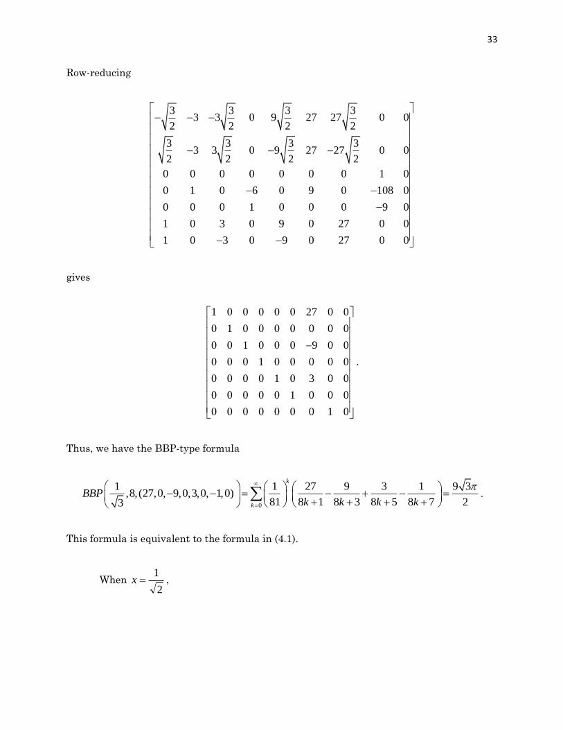
33
Row-reducing
3 3 3 33 3 0 9 27 27 0 0
2 2 2 2
3 3 3 33 3 0 9 27 27 0 0
2 2 2 2
0 0 0 0 0 0 0 1 0
0 1 0 6 0 9 0 108 0
0 0 0 1 0 0 0 9 0
1 0 3 0 9 0 27 0 0
1 0 3 0 9 0 27 0 0
gives
1 0 0 0 0 0 27 0 0
0 1 0 0 0 0 0 0 0
0 0 1 0 0 0 9 0 0
0 0 0 1 0 0 0 0 0
0 0 0 0 1 0 3 0 0
0 0 0 0 0 1 0 0 0
0 0 0 0 0 0 0 1 0
.
Thus, we have the BBP-type formula
0
1 1 27 9 3 1 9 3,8,(27,0, 9,0,3,0, 1,0)
81 8 1 8 3 8 5 8 7 23
k
k
BBPk k k k
.
This formula is equivalent to the formula in (4.1).
When 2
1x ,

34
.2
11ln)842(
2
11ln)842(2ln645ln)168442(
3ln2)842(2
1arctan22)842(
)2arctan(2)88422(
2)4(8
1),,,,,,,(,8,
2
1
7531
75318875431
86427531
765321
6287654321
aaaa
aaaaaaaaaaa
aaaaaaaa
aaaaaa
aaaaaaaaaaBBP
.
Row-reducing
008040201
0168044201
080402010
010000000
008040201
008840221
we get
000000000
000110000
004201000
004000100
008000010
000400001
.
This gives two BBP-type formulas,
0 68
1
58
1
48
2
18
4
16
1)0,0,1,1,2,0,0,4(,8,
2
1
k
k
kkkkBBP
which is the original BBP formula (1.1), and

35
0
278
1
48
4
38
4
28
8
16
1)0,1,0,0,4,4,8,0(,8,
2
1
k
k
kkkkBBP .
When 1x , ),,,,,,,(,8,1 87654321 aaaaaaaaBBP only converges if
087654321 aaaaaaaa . Using this,
.)22ln(222ln2
2ln232
)(16
1),,,,,,,(,8,1
75317531
8754317531
76532187654321
aaaaaaaa
aaaaaaaaaa
aaaaaaaaaaaaaaBBP
Row-reducing
1 0 1 1 1 0 1 3 0
1 0 1 0 1 0 1 0 0
1 0 1 0 1 0 1 0 0
1 1 1 1 1 1 1 1 0
yields
1 31 0 0 0 0 1 0
2 2
0 1 0 2 0 1 0 4 0
1 30 0 1 1 0 0 0
2 2
0 0 0 0 0 0 0 0 0
.
Thus, we have the BBP-type formulas,
(6.1) , 8
)423(
88
2
38
3
28
8
18
3)2,0,0,0,0,3,8,3(,8,1
0
k kkkkBBP
36
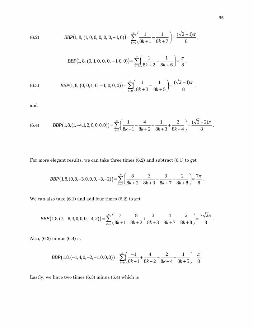
(6.2) 8
)12(
78
1
18
1)0,1,0,0,0,0,0,1(,8,1
0
k kkBBP ,
868
1
28
1)0,0,1,0,0,0,1,0(,8,1
0
k kkBBP ,
(6.3) 8
)12(
58
1
38
1)0,0,0,1,0,1,0,0(,8,1
0
k kkBBP ,
and
(6.4) 0
1 4 1 2 ( 2 2)1,8,(1, 4,1,2,0,0,0,0)
8 1 8 2 8 3 8 4 8k
BBPk k k k
.
For more elegant results, we can take three times (6.2) and subtract (6.1) to get
0
8 3 3 2 71,8,(0,8, 3,0,0,0, 3, 2)
8 2 8 3 8 7 8 8 8k
BBPk k k k
.
We can also take (6.1) and add four times (6.2) to get
0
7 8 3 4 2 7 21,8,(7, 8,3,0,0,0, 4,2)
8 1 8 2 8 3 8 7 8 8 8k
BBPk k k k k
.
Also, (6.3) minus (6.4) is
0
1 4 2 11,8,( 1,4,0, 2, 1,0,0,0)
8 1 8 2 8 4 8 5 8k
BBPk k k k
.
Lastly, we have two times (6.3) minus (6.4) which is

37
0
1 4 1 2 2 21,8,( 1,4,1, 2, 2,0,0,0)
8 1 8 2 8 3 8 4 8 5 8k
BBPk k k k k
.
For the alternating case, we have eliminated the several pages of the integration.
),,,,,,,(,8, 87654321 aaaaaaaaxABBP involves the following arctangents
22
222arctan
x,
22
222arctan
x,
22
222arctan
x,
and
22
222arctan
x.
These arctangents evaluate if 1x as follows
2 2 2arctan
162 2
,
2 2 2 7arctan
162 2
,

38
2 2 2 3arctan
162 2
,
and
2 2 2 5arctan
162 2
.
Using this information we were able to simplify ),,,,,,,(,8,1 87654321 aaaaaaaaABBP . To
eliminate the logarithms we row-reduced
5 50 2 2 0 0 0 2 2 0 (1 2) 2 2 0
4 4
1 1 1 1 1 11 2 2 0 2 2 1 2 2 0
4 42 2 2 2
1 1 1 1 1 11 2 2 0 2 2 1 2 2 0
4 42 2 2 2
3 1 1 32 0 1 0 1 0 2 0 0
2 2 2 2
3 1 1 32 0 1 0 1 0 2 0 0
2 2 2 2
,
which yields
1 0 0 0 0 0 1 0 0
0 1 0 0 0 1 0 0 0
0 0 1 0 1 0 0 0 0
0 0 0 0 0 0 0 1 0
0 0 0 0 0 0 0 0 0
.
This leads to the following BBP-type formulas
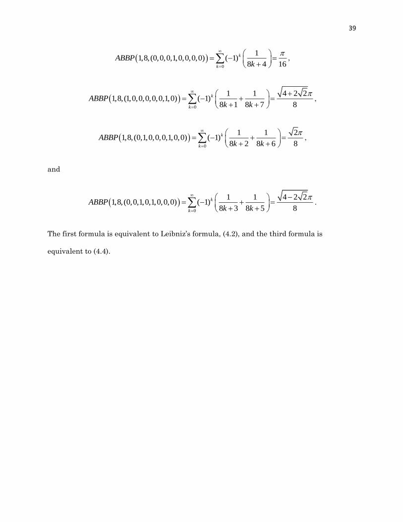
39
0
11,8,(0,0,0,1,0,0,0,0) ( 1)
8 4 16
k
k
ABBPk
,
0
1 1 4 2 21,8,(1,0,0,0,0,0,1,0) ( 1)
8 1 8 7 8
k
k
ABBPk k
,
0
1 1 21,8,(0,1,0,0,0,1,0,0) ( 1)
8 2 8 6 8
k
k
ABBPk k
,
and
0
1 1 4 2 21,8,(0,0,1,0,1,0,0,0) ( 1)
8 3 8 5 8
k
k
ABBPk k
.
The first formula is equivalent to Leibniz’s formula, (4.2), and the third formula is
equivalent to (4.4).

40
Chapter 7: Conclusions
In this project, I focused on BBP-type formulas for scaled values of . It might be
interesting to carry out this algorithm for other constants, such as arctangents, logarithms,
and zero. The constant zero relates the null space of the system of linear equations. Except
for an example in the alternating base 4 case and base 8 cases, our method only utilized a
single arctangent term. Since there are many formulas for combinations of arctangents,
like
24
3arctan
2
1arctan2
.
A more sophisticated approach would take this into account.
BBP-type formulas can be extended to the formulas of the form
s
n
sk
s
nk
nnk
a
nk
a
nk
ax
)()2()1(
2
0
1
where s is an integer. This form leads to BBP-type formulas for constants such as 2 , as in
the following example,
2
220
22222 )78(
2
)68(
4
)58(
4
)48(
16
)38(
8
)28(
16
)18(
16
16
1
kkkkkkkk
k
,
from [3, p. 8 formula 19]. Our algorithm handles only cases where 1s . Future work
could explore this area.
From [7, p. 737], we have the equation

41
0 0
1 1 1 1 32 8 14
4 2 1 64 1024 4 1 4 2 4 3
k k
k kk k k k
.
The above formula allows for the individual hex or binary digits of to be calculated. It is
over 40% faster than formula (1.1). It would be of interest to search for a faster equation or
of BBP-type formulas that are combinations of different bases with different x -values.
Another limitation to our algorithm is that as we increase the base, we complicate
the integration. Base 8 is the highest case that our algorithm can handle without too much
complexity. Base 12 appears to have BBP-type formulas; it would have been nice to take a
closer look at it.
Our algorithm is useful as it is a combination of elementary concepts. We simply
used Theorem 1 and 2, along with row-reducing matrices of systems linear equations to
eliminate non- constants. Also, using integration provided a useful tool in discovering
“nice” x-values. Although our algorithm for searching for BBP-type formulas does not work
well for higher bases, it does work well for verifying most cases previously discovered of
degree one.

42
References
[1] S. Abbott, Understanding Analysis, Springer, New York, 2001.
[2] J. Arndt and C. Haenel, Pi – Unleashed, Springer, Berlin, 2001.
[3] D. Bailey, “A Compendium of BBP-Type Formulas for Mathematical Constants,” 2004,
available at http://crd.lbl.gov/~dhbailey/dhbpapers/bbp-formulas.pdf.
[4] D. Bailey and J. Borwein, Mathematics by Experiment: Plausible Reasoning in the 21st
Century, A K Peters, MA, 2004.
[5] D. Bailey, P. Borwein, and S. Plouffe, “On the Rapid Computation of Various
Polylogarithmic Constants,” Mathematics of Computation, vol. 66, no. 218, 1997, p.
903-913.
[6] P. Beckmann, A History of Pi, The Golem Press, Boulder, CO, 1971.
[7] L. Berggren, J. Borwein, and P. Borwein, Pi: A Source Book, 3rd ed., Springer, New
York, 2004.
[8] I. Lehmann and A. S. Posamentier, A Biography of the World’s Most Mysterious
Number, Prometheus Books, Amherst, NY, 2004.
[9] J. Stewart, Calculus: Concepts and Contexts, 2nd ed., Brooks/Cole, Pacific Grove, CA,
2001.
[10] http://en.wikipedia.org/wiki/Bailey-Borwein-Plouffe_formula
[11] http://mathworld.wolfram.com/BBP-typeFormula.html

43
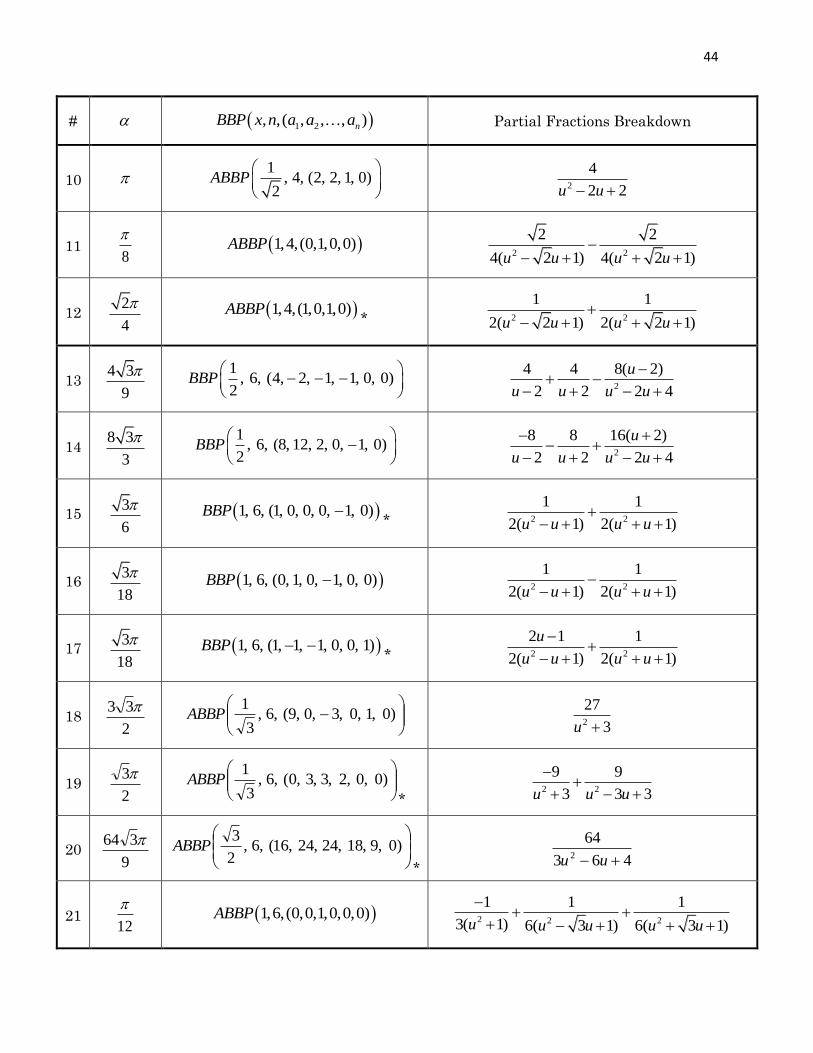
Appendix 1: Table Summarizing Bases 2, 3, 4, 5, 6, and 8
The following table summarizes the results of BBP-type formulas discovered in
chapters 4, 5, and 6.
Table 3- BBP-type formulas discovered
#
1 2, , ( , , , )nBBP x n a a a Partial Fractions Breakdown
1 6
1, 2, (1, 0)
3ABBP
2
3
3u
2 4
1, 2, (1,0)ABBP
2
1
1u
3 9
3
1, 3, (1, 1, 0)BBP
*
2
1
1u u
4 4 3
9
1, 3, (2, 1, 0)
2ABBP
*
2
8
2 4u u
5 2 3
9
1, 3, (1, 1, 0)ABBP
*
2
1
1u u
6 3
9
1, 3, (1, 0, 1)ABBP
*
2
1
1
u
u u
7 3
2
1, 4, (3, 0, 1, 0)
3BBP
2
9
3u
8 4
1, 4, (1, 0, 1, 0)BBP
2
1
1u
9 4
1, 4, (2, 3, 0, 1)BBP
*
2
1 2 1
1 1
u
u u
44
#
1 2, , ( , , , )nBBP x n a a a Partial Fractions Breakdown
10
1, 4, (2, 2, 1, 0)
2ABBP
2
4
2 2u u
11 8
1,4,(0,1,0,0)ABBP
2 2
2 2
4( 2 1) 4( 2 1)u u u u
12 2
4
1,4,(1,0,1,0)ABBP
*
2 2
1 1
2( 2 1) 2( 2 1)u u u u
13 4 3
9
1, 6, (4, 2, 1, 1, 0, 0)
2BBP
2
4 4 8( 2)
2 2 2 4
u
u u u u
14 8 3
3
1, 6, (8, 12, 2, 0, 1, 0)
2BBP
2
8 8 16( 2)
2 2 2 4
u
u u u u
15 3
6
1, 6, (1, 0, 0, 0, 1, 0)BBP
*
2 2
1 1
2( 1) 2( 1)u u u u
16 3
18
1, 6, (0, 1, 0, 1, 0, 0)BBP
2 2
1 1
2( 1) 2( 1)u u u u
17 3
18
1, 6, (1, 1, 1, 0, 0, 1)BBP
*
2 2
2 1 1
2( 1) 2( 1)
u
u u u u
18 2
33
)0,1,0,3,0,9(,6,
3
1ABBP
2
27
3u
19 2
3
)0,0,2,3,3,0(,6,
3
1ABBP
* 2 2
9 9
3 3 3u u u
20 9
364
)0,9,18,24,24,16(,6,
2
3ABBP
* 463
642 uu
21 12
1,6,(0,0,1,0,0,0)ABBP
2 2 2
1 1 1
3( 1) 6( 3 1) 6( 3 1)u u u u u

45
#
1 2, , ( , , , )nBBP x n a a a Partial Fractions Breakdown
22 3
1,6,(1,0,0,0,1,0)ABBP
*
2 2 2
2 1 1
3( 1) 6( 3 1) 6( 3 1)u u u u u
23 3
9
1,6,(0,1,0,1,0,0)ABBP
)13(6
3
)13(6
322
uuuu
24 3
18
1,6,(0,1,0,0,0, 1)ABBP
2 2
3 2 3 3 2 3
6( 3 1) 6( 3 1)
u u
u u u u
25 9 3
2
1,8,(27,0, 9,0,3,0, 1,0)
3BBP
2
81
3u
26
)0,0,1,1,2,0,0,4(,8,
2
1BBP
2 2
4 4( 2)
2 2 2
u u
u u u
27 2
)0,1,0,0,4,4,8,0(,8,
2
1BBP
2 2
8 8
2 2 2
u
u u u
28 7
8
1,8,(0,8, 3,0,0,0, 3, 2)BBP *
2 2 2
3 5 3 2 3 2 3
2( 1) 2( 1) 4( 2 1) 4( 2 1)
2 2u u u
u u u u u u
29 7 2
8
1,8,(7, 8,3,0,0,0, 4,2)BBP * 2 2 2
3 5 4 2 7 3 2 2 7 3 2
2( 1) 2( 1) 4( 2 1) 4( 2 1)
u u u
u u u u u u
30 8
)0,0,1,0,0,0,1,0(,8,1 BBP
2 2
2 2
4( 2 1) 4( 2 1)u u u u
31 8
1,8,( 1,4,0, 2, 1,0,0,0)BBP
* 2 2 2
1 3 1 2 3 2 3
2( 1) 2( 1) 4( 2 1) 4( 2 1)
2 2u u u
u u u u u u
32 2
8
1,8,( 1,4,1, 2, 2,0,0,0)BBP
* 2 2 2
1 3 2 2 1 3 2 1 3
2( 1) 2( 1) 4( 2 1) 4( 2 1)
2 2u u u
u u u u u u

46
#
1 2, , ( , , , )nBBP x n a a a Partial Fractions Breakdown
33 16
1, 8, (0, 0, 0, 1, 0, 0,0, 0)ABBP
1222
1
1222
1
1222
1
1222
1
2244
1
uuuu
uuuu
34 4 2 2
8
1, 8, (1, 0, 0, 0, 0, 0,1, 0)ABBP*
1222
12
1222
12
1222
21
)1222(2
22
24
1
uuuu
uuuu
35 2
8
1, 8, (0, 1, 0,0, 0, 1,0, 0)ABBP
1222
1
1222
1
1222
22
1222
1
224
1
uuuu
uuuu
36 4 2 2
8
1, 8, (0, 0,1,0, 1, 0,0, 0)ABBP*
1222
1
1222
1
1222
1
1222
1
24
1
uuuu
uuuu
We will refer to each formula by its number corresponding to the first column.
Formulas 1, 7, 18, and 25 are equivalent to the power series of
3
1tan .
Formulas 2, 8, 11, 21, 30, and 33 are equivalent to Leibniz’s Formula, (4.2).
Formulas 3 and 16 are equivalent.
Formulas 5 and 23 are equivalent.
Formulas 6 and 24 are equivalent.
Formulas 10, 13, and 14 can be found in [3, p. 7 formula 16 and p. 16 formulas 58 & 59
respectively].
Formulas 12 and 35 are equivalent.
Formulas 26 and 27 can be found in [11, formulas 2 & 3 respectively].
Formulas 3, 4, 5, 6, 9, 12, 15, 17, 19, 20, 22, 28, 29, 31, 32, 34, and 36 are possibly new BBP-
type formulas as we did not see them in the literature. They are also marked with an * in
the above table. If two formulas are equivalent, only the formula from with a smaller base
is considered new.

47
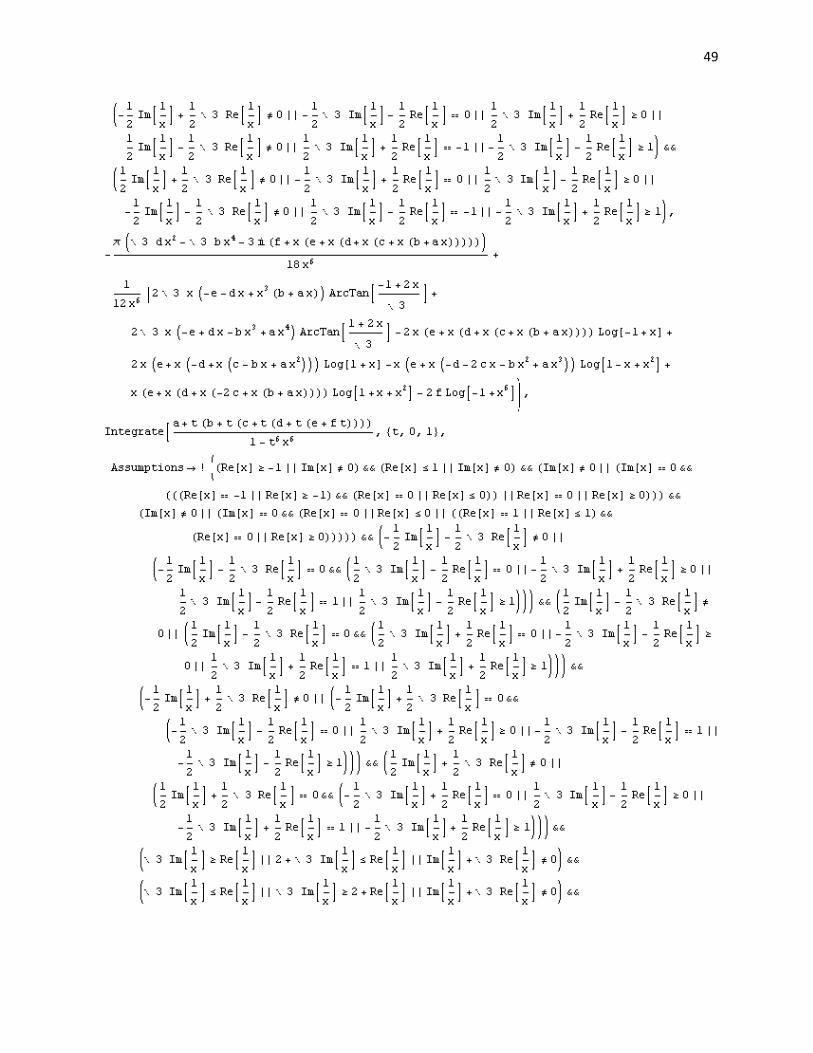
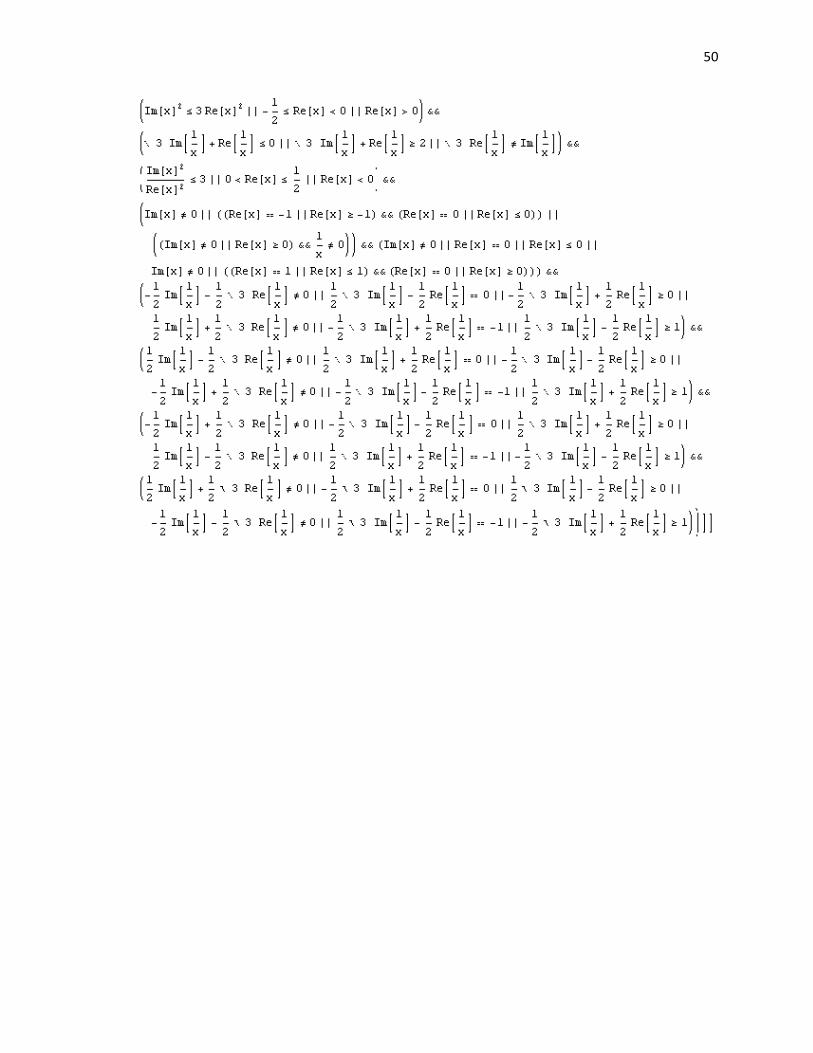
Appendix 2: Mathematica’s Output for the Non-Alternating Base 6
This is the actual Mathematica output for integrating the non-alternating base 6
case. The restrictions on x can be disregarded since we are concerned with 1x and
when 1x we add the necessary constraints. Also, ,,,,, edcba and f are equivalent to
,,,,, 54321 aaaaa and 6a respectively. For simplification, expressions were expanded and
constants were factored. Logarithms were also expanded, i.e. 62 Log 1f x is
equivalent to 6
62 ln( 1 )a x , which was expanded to
2 2
62 ln 1 ln( 1) ln( 1) ln( 1)a x x x x x x .
This often affected the system of linear equations and added a degree of freedom. Similar
simplification was used once an x –value was plugged in.
In the base 8 case, partial fractions were used to convert the integral into four
integrals. The four integrals were integrated separately and their results were summed
together.

48
49
50